unit roots, cointegration and pre-testing in var modelsecondept/workshops/spring_2013... ·...
TRANSCRIPT
Unit Roots, Cointegration and Pre-Testing in VAR
Models∗
Nikolay Gospodinov†
Concordia University,
CIRANO and CIREQ
Ana María Herrera‡
University of Kentucky
Elena Pesavento§
Emory University
February 2013
Abstract
This chapter investigates the robustness of impulse response estimators to near unit roots
and near cointegration in VAR models. We compare estimators based on VAR specifications
determined by pre-tests for unit roots and cointegration as well as unrestricted VAR specifi-
cations in levels. Our main finding is that the impulse response estimators obtained from the
levels specification tend to be most robust when the magnitude of the roots is not known. The
pre-test specification works well only when the restrictions imposed by the model are satisfied.
Its performance deteriorates even for small deviations from the exact unit root for one or more
model variables. We illustrate the practical relevance of our results through simulation examples
and an empirical application.
∗We would like to thank the participants at the 12th Annual Advances in Econometrics Conference for useful
feedback. We are particularly indebted to Lutz Kilian for numerous detailed comments and insightful suggestions
that substantially improved the presentation of the chapter. Nikolay Gospodinov gratefully acknowledges financial
support from FQRSC and SSHRC.
†Department of Economics, Concordia University, Montreal, QC H3G 1M8, Canada; e-mail:
‡Department of Economics, University of Kentucky, Lexington, KY 40506-0034, USA; e-mail: [email protected]
§Department of Economics, Emory University, Atlanta, GA 30322-2240, USA; e-mail: [email protected]
1 Introduction
Most economic variables that are used for policy analysis and forecasting are characterized by
high persistence and possibly nonstationary behavior. It is common practice in applied work to
subject these series to pre-tests for unit roots and cointegration prior to the vector autoregressive
(VAR) analysis to determine the appropriate transformations that render the data stationary.
Incorporating information about the integration and cointegration properties of the data in VAR
models reduces the estimation uncertainty and the degree of small-sample bias of impulse response
estimates. Such pre-tests, however, suffer from lack of robustness for small deviations from unit
roots and cointegration. For example, Gospodinov, Maynard and Pesavento (2011) demonstrate
that arbitrarily small deviations from an exact unit root may produce impulse response estimators
that are highly distorted and misleading. The main goal of this article is to study and quantify the
role of pre-tests for unit roots and cointegration for VAR specifications and identification schemes
for impulse response analysis. We contrast the pre-test approach to the specification of VAR
models with the alternative of expressing all VAR variables in levels. The latter practice, which is
also common in applied work, is susceptible to problems of small-sample bias, especially when the
data are highly persistent. Moreover, it requires appropriate choices of bootstrap or asymptotic
methods for inference that are developed to accommodate near-integrated processes. However,
the levels specification makes the estimates of structural impulse responses, identified by short-run
restrictions, asymptotically robust to the unknown order of integration of the model variables. The
relative merits of the pre-test VAR approach and the levels approach for VAR impulse response
analysis are not well understood. The objective of this article is to examine this issue and to provide
users of VAR models with advice on how to proceed in practice.
The limitations of the pre-test approach to VAR specification were first discussed more than a
decade ago. Elliott (1998) illustrated the possibly large size distortions of the cointegration methods
that arise in systems with near unit roots. It is widely documented that similar distortions tend to
characterize the properties of sequential modeling and specification procedures that are based on
pre-tests for unit roots. These tests are known to have low power in rejecting the null of a unit root
when the data are highly persistent and nearly integrated. Nevertheless, Elliott’s (1998) warning
has been ignored by many applied researchers who continue to rely on pre-tests, perhaps because of
the perception that the levels specification is not without its own potential drawbacks. This article
1
examines how severe the problem documented by Elliott (1998) is for estimators of VAR impulse
responses and which of the commonly used approaches to determining the VAR specification is
most accurate in practice. We conduct a Monte Carlo study that assesses the mean squared errors
(MSEs) of selected impulse response estimates and quantify how dangerous the pre-test strategy can
be in practice. The pre-tests include individual unit root tests such as the augmented Dickey-Fuller
test with GLS detrending (ADF-GLS) and tests for cointegrating rank, which determine whether
the model should be estimated as a VAR in differences, a vector error-correction model (VECM)
or a VAR in levels. Our simulation results provide support for the robustness of the level VAR
specification to departures from exact unit roots and cointegration and to the possible presence of
unmodelled low frequency co-movement among the variables of interest.
Our evidence in favor of the levels specification highlights the importance of valid inference
on impulse response estimators when there is uncertainty about the integration and cointegration
properties of the data. We provide a brief review of several asymptotic and bootstrap approaches
and methods for inference in levels models including local-to-unity asymptotics (Gospodinov, 2004,
2010; Mikusheva, 2012; Pesavento and Rossi, 2006; Phillips, 1998), delta method asymptotics (Sims,
Stock, and Watson, 1990), and bootstrap asymptotics (Kilian, 1998; Inoue and Kilian, 2002). We
show that the best approach may differ depending on the properties of the data, the dimensionality
of the system, the forecast horizon, the identification scheme, etc.
The remainder of this chapter is structured as follows. Section 2 provides a short description of
various representations of multivariate integrated processes. The following section introduces the
common trend decomposition for nearly integrated process and discusses some theoretical results
for impulse response analysis with nearly integrated (and possibly cointegrated) processes based
on short-run and long-run identifying restrictions. Section 4 reviews the theoretical literature on
inference for impulse response functions which is robust to the magnitude of the largest roots of
the process. Section 5 presents the results of several simulation exercises. Section 6 concludes.
2
2 A Brief Review of Representations of Multivariate Integrated
Processes
Let yt be an I(1) multivariate (m× 1) process. Since ∆yt is I(0) by assumption, ∆yt has a moving
average (MA) representation of the form
∆yt = C(L)ut, (1)
where C(L) = C0 + C1L+ C2L2 + ... is a m×m matrix lag polynomial and ut ∼ iid(0,Ω). Then,
∆yt has a long-run covariance matrix Ω = C(1)ΣC(1)′.
For any β 6= 0m×r (r = 1, ...,m), the long-run variance of β′∆yt is β′Ωβ = β′C(1)ΣC(1)′β. If β
are r cointegrating vectors of dimension m× 1, then β′yt is I(0) and β′∆yt is overdifferenced with
a zero long-run variance. Therefore, for β to be cointegrating vectors, we must have
β′C(1)ΣC(1)′β = 0.
This expression cannot equal zero if C(1) has full rank. Thus, cointegration requires C(1) to have
rank less than m and β must lie in the null space of C(1), i.e., so that β′C(1) = 0r×1.
Assuming that C(L) is invertible, model (1) has the VAR representation
A(L)yt = ut, (2)
where A(L) = (1−L)C(L)−1 is a p-th order lag polynomial. Evaluating (1−L)Im = A(L)C(L) at
L = 1 yields
A(1)C(1) = 0m×m.
Therefore, A(1) lies in the null space of C(1) and, from the previous results for the MA represen-
tation, must be a linear combination of the cointegrating vectors β. More precisely, A(1) = −αβ′,
where α is an m× r matrix of rank r and β is m× r.
Finally, model (2) admits an VECM representation
∆yt = Πyt−1 + Γ(L)∆yt + et,
where Γ (L) = Γ1L + Γ2L2 + ... + Γp−1Lp−1, Γi = −
∑pj=i+1Aj and Π = −A(1) = αβ′. In this
representation, rank(Π) = r < m, i.e., Π has a rank which is less than its dimension if there are r
cointegrating relations. If rank(Π) = m, all elements of yt are I(0) and the appropriate model is an
3
unrestricted VAR in levels; whereas if rank(Π) = 0, all elements of yt are I(1) and not cointegrated,
and the appropriate model is VAR in first differences. Practitioners are commonly faced with the
decision of which of these three models (VAR in levels, VAR in first differences, or VECM) to
estimate, and this decision is often made on the basis of pre-tests for unit root and cointegration.
A second issue faced by practitioners interested in identifying the effect of a structural shock of
interest (e.g., monetary policy shocks, oil price shocks, or technological innovations ) is the choice of
identifying restrictions. In the applied literature, the most commonly used identification strategies
are short-run and long-run restrictions. Short-run identification schemes can be characterized as
follows. Let B0 denote an m×m invertible matrix with ones on the main diagonal. Pre-multiplying
both sides of (2) by B0 yields the structural VAR (SVAR) model
B(L)yt = εt,
where B(L) = B0A(L) and εt = B0ut denote the structural shocks which are assumed to be
orthogonal with a diagonal covariance matrix Σ. Hence,
E(utu′t) ≡ Ω = B−10 ΣB−1′0 .
Given that Ω is symmetric with m(m+1)2 , in order to identify all the elements of B0 we need to impose
m(m−1)2 restrictions. One possibility is to restrict B0 to be lower triangular which is equivalent to
a Choleski decomposition of Ω. Note that the short-run identifying restrictions do not depend on
the specification of the reduced-form VAR model (e.g., Lütkepohl and Reimers, 1992).
Alternatively, one can impose long-run identifying restrictions that render the moving average
matrix A(1)−1B−10 lower triangular. The use of long-run restrictions is less general in that it re-
quires some model variables to be I(1) and others to be I(0), making this approach particularly
susceptible to any misspecification of the integration properties of the individual series. For exam-
ple, Gospodinov, Maynard and Pesavento (2011) demonstrate that even arbitrary small deviations
from the exact unit, when combined with long run identification restrictions, can produce impulse
response estimates that are highly distorted.
In Section 4 we study how alternative choices of model specification and identification restric-
tions can affect the MSE of the structural impulse responses.
4
3 Some Theoretical Results for Near-Integrated Processes
In this chapter, our main interest lies in data generating processes (DGPs) in which the variables
in the VAR are highly persistent with roots that are either close to one or equal to one.1 This is
the typical situation a practitioner estimating a VAR with macroeconomic variables would face.
Theoretically, these variables are well approximated by near-integrated processes. Thus, to under-
stand the effect of persistent variables on the estimation of the VARs, we start by reviewing some
theoretical results for near-intergrated processes.
3.1 Common trend decomposition of near-integrated processes
Let yt denote a multivariate m× 1 process
(Im − ΦL)yt = Ψ(L)et,
where Φ = Im + C/T and C is a matrix of fixed constants. It is often convenient to define
C = diag(c1, c2, ..., cm) in order to rule out I(2) processes when the diagonal elements are zero. We
discuss the effect of non-zero off-diagonal elements later. Assume that y0 = 0; Ψ(L) =∑∞
i=0 ΨiLi
with Ψ0 = Im,∑∞
i=0 i|Ψi| < ∞ and∑∞
i=0 Ψi 6= 0m×m; and et is a homoskedastic martingale
difference sequence with a covariance matrix Σ and finite fourth moments. Deterministic terms are
assumed away for notational convenience.
Let ut = Ψ(L)et. Then, ut = [Ψ(1)+(1−L)Ψ∗(L)]et by the Beveridge-Nelson (BN) decomposi-
tion, where Ψ(1) =∑∞
i=0 Ψi, Ψ∗(L) =∑∞
i=1 Ψ∗iLi−1 and Ψ∗i = −
∑∞j=i Ψj . Denoting St =
∑tj=1 et
and using recursive substitution and summation by parts,
yt =t∑
j=1
Φt−jΨ(L)ej = Ψ(1)St + vt +C
T
t−1∑j=1
Ψ(1)Φt−jSj−1 +C
T
t−1∑j=1
Φt−jvj−1, (3)
where vt = Ψ∗(L)et.
Expression (3) is an algebraic decomposition (or factorization) of the process yt that contains
the standard BN decomposition for exact unit root processes as a special case (C = 0m×m). While
the standard BN decomposition is given by the permanent, Ψ(1)St, and transitory, vt, components,
the decomposition in (3) contains two additional terms. The fourth term CT
∑t−1j=1 Φt−jvj−1 is
1Persistent variables can also be approximated by fractionally integrated processes. Allowing for this possibility is
outside the scope of this chapter, although some of the results in our simulations may generalize to the case in which
the DGP contains fractionally intergrated variables.
5
asymptotically negligible, whereas the term CT
∑t−1j=1 Ψ(1)Φt−jSj−1 is not and is of the same order
Op(T1/2) as Ψ(1)St. Therefore, (3) contains two permanent component terms (i.e., two terms of
order Op(T 1/2)). Omitting one of the them (by wrongly assuming an exact unit root, for example)
will cause misspecification bias and undermine the size of hypothesis tests.
Consider, for example, the cointegration model (Elliott, 1998)
y1,t = βy2,t + u1,t
y2,t = (1 + c/T )y2,t−1 + u2,t,
which can be cast in a similar representation as the model above. In this case, the restriction
βΨ(1) = 0 does not annihilate the permanent component. As a result, reduced rank regressions
that impose only this restriction are not valid and would cause misspecification bias and test size
distortions as shown by Elliott (1998). Similar misspecification biases are expected to play a role
in impulse response analysis based on long-run identifying restrictions on Ψ(1), i.e., restrictions
imposed on the ’wrong’permanent component when C 6= 0m×m.
In brief, wrongly assuming that a multivariate process yt has one or more unit roots, when the
roots are close but not equal to unity, leads to distortions in reduced rank regressions, as well as in
the BN decomposition and impulse response analysis.
3.2 Impulse response analysis in VAR models with near unit roots identified
by short-run restrictions
Let the data generating process be given by
A(L)yt = et (4)
or
(Im − ΛL) = Ψ(L)et,
where A(L) = Im− A1L− ...− ApLp has roots outside or on the unit circle, and Λ can be expressed
in terms of its eigenvalues and eigenvectors as Λ = V −1ΦV with Φ as defined above (Pesavento and
Rossi, 2006). This model allows for unit roots and possible cointegration and several representations
in other parts of the chapter can be regarded as specifications in the rotated variables yt = V yt
and et = V et.
6
Despite the possible presence of unit roots and cointegration, the estimates of A1, ..., Ap from
the levels VAR (4) are root-T consistent and individually normally distributed (Sims, Stock and
Watson, 1990). Using these estimates and a short-run (recursive) identification scheme, one can
construct l-period ahead orthogonalized impulse responses Θl. Provided that the response horizon
is fixed with respect to the sample size, the impulse response estimators are, under weak condi-
tions, consistent and asymptotically normally distributed (see Lütkepohl and Reimers, 1992). This
explains the robustness of impulse response estimators based on the level specification to possible
deviations from exact unit roots and cointegration, as long as the structural parameters and shocks
are identified using short-run restrictions. In contrast, inference becomes nonstandard if we rely
on long-run restrictions for identification, as discussed below. A similar problem would arise, re-
gardless of the identification, if we allowed the response horizon to grow fast enough with respect
to the sample size. The latter result casts doubt on impulse response estimates for long horizons
when the data are persistent. Indeed, Kilian and Chang (2000) document that the reliability of im-
pulse response estimates from standard levels specifications may deteriorate substantially at longer
horizons.
3.3 Impulse response analysis in VAR models with near unit roots identified
by long-run restrictions
This case is best illustrated in the context of the Blanchard and Quah (1989) model for which
yt = (4Yt, Ut)′, where Yt is the output (log real GNP) and Ut is the unemployment rate, A(L) =
Ψ(L)−1(I2 −ΦL) and B0 =
1 −b(0)12−b(0)21 1
. The structural shocks εt = B0et can be interpreted
as aggregate supply and demand shocks (εst , εdt )′. The long-run identifying restriction that the
demand shocks εdt have no long-run effect on output imposes a lower triangular structure on the
moving average matrix A(1)−1B−10 . Hence, under this identifying restriction, the matrix of long-run
multipliers in the structural model, B(1) = B0A(1), is also lower triangular.
The robustness of the impulse response analysis depends crucially on the persistence of Ut and,
hence, on the parameterization of the matrix Φ. We follow Gospodinov, Maynard and Pesavento
(2011) and express Φ as Φ =
1 δ
0 ρ
, where δ = −γ (1− ρ) is the parameter that determines
the low frequency co-movement between the variables, and ρ = 1 + c/T (for c < 0) denotes the
largest root of the unemployment rate. The non-zero off-diagonal element γ (1− ρ) allows for the
7
possibility that a small low frequency component of unemployment affects output growth.
To gain some further insight into this parameterization, let us assume for simplicity that Ψ(L) =
I2 and note that the vector error-correction form of the model is given by
4yt = (ρ− 1)
0 −γ
0 1
yt−1 + et,
which can be written as
4yt = αβ′yt−1 + et,
where α = (ρ− 1)
γ
1
and β = (0, 1)′. Therefore, the model has a trivial cointegration vector
(0, 1)′ and the speed of adjustment α is a function of γ which carries important information from
the levels of the series, provided that ρ < 1.
With this parameterization of Φ, the long-run multiplier matrix is given by
B(1) =
ψ11(1)− b(0)12 ψ21(1) (1− ρ)(
[γψ11(1) + ψ12(1)]− b(0)12 [γψ21(1) + ψ22(1)])
ψ21(1)− b(0)21 ψ11(1) (1− ρ)(
[γψ21(1) + ψ22(1)]− b(0)21 [γψ11(1) + ψ12(1)]) ,
where ψij(1) denotes the corresponding elements of the matrix Ψ(1)−1. Imposing the long-run
restriction that aggregate demand shocks have no permanent effect on output implies that b(0)12 =
[γψ11(1) + ψ12(1)]/[γψ21(1) + ψ22(1)]. In contrast, imposing a unit root in unemployment (ρ = 1)
and differencing both output and unemployment renders the restriction b(0)12 = ψ12(1)/ψ22(1). Thus,
the differenced VAR ignores any information contained in the levels of output and unemployment.
The main message to the practitioner is that the differenced VAR specification is not robust to
small low frequency co-movements. While the levels specification (in which some of the variables
are in first differences and some are in levels) preserves the information on the low-frequency co-
movement, the estimates of the impulse response functions are inconsistent and their distribution is
fat-tailed in the presence of local-to-unity processes (Gospodinov, 2010). In summary, the applied
researchers should exert extreme caution when working with near-integrated variables and the
SVAR is identified by long-run restrictions.
3.3.1 Unit root pre-test VAR specification
Similarly to the case of the differenced VAR, lack of robustness is expected to characterize the
behavior of specifications based on pre-test for a unit root given that this pre-test will select the
8
differenced specification with probability approaching one when the process is near-integrated.
Hence, the unit root pre-test VAR specification will inherit the non-robustness properties of the
differenced VAR specification for slowly co-moving, near-integrated variables.
4 Robust inference for impulse response functions
Given the low power of most pre-tests for unit root and cointegration, and costs from estimating
a VAR that erroneously imposes unit roots, the current literature has moved in the direction of
methods for inference that are robust to possible presence of unit roots. These robust methods are
designed for VAR models based on short-run identifying restrictions only, of course, as departures
from exact unit roots immediately invalidate the use of long-run identifying restrictions. Consider
the model
(Im − ΦL)yt = Ψ(L)et,
where Φ = Im + C/T and C = diag(c1, c2, ..., cm). Note that yt could denote rotated variables to
account for the possibility of cointegration with a known cointegration vector (for more details, see
Pesavento and Rossi, 2006). Suppose that the interest lies in inference on the impulse responses of
yt at long response horizons l, yt+l, to the structural shocks εt = B0et.
To better capture the uncertainty in estimating the impulse responses at long horizons, it is
convenient to parameterize l as a function of the sample size. More specifically, let l = [δT ] for
some fixed δ > 0. Under this parameterization, we have that C l → eCδ as T → ∞, where eδC
is a diagonal matrix with (eδc1 , eδc2 , ..., eδcm) on the main diagonal (Pesavento and Rossi, 2006;
Gospodinov, 2004). Furthermore,
Θl ≡∂yt+l∂et
= Φl(Im + Φ−1Ψ1 + Φ−1Ψ2 + ...) + o(1) ' ΦlΨ(1) (5)
and the l-period impulse response function of the j-th variable in yt to the k-th structural shock in
εt is given by (Pesavento and Rossi, 2006)
∂yj,t+l∂εk,t
' ι′jΦlΨ(1)B−10 ιk → ι′jeCδΨ(1)B−10 ιk (6)
as T → ∞, where ιj and ιk are the corresponding columns of the identity matrix Im. Inference
on the impulse response function can then proceed by plugging a consistent estimate of Ψ(1) and
obtaining the confidence interval limits for the localizing constant cj of the j-th variable yj,t, which
9
is typically done by inverting a unit root test (see, for example, Stock, 1991). In this sense, this
method is a two-step procedure, which involves the construction of a confidence interval for cj in
the first step and using this confidence interval and the expression (6) to construct a confidence
interval for the impulse response function ∂yj,t+l∂εk,t
.
Gospodinov (2004) proposes a one-step test-inversion method for directly constructing confi-
dence bands for the impulse response function. Let θ = (vec(Φ)′, vec(Ψ1)′, vec(Ψ2)
′, ...)′, where in
practice Ψ1,Ψ2, ... are approximated by a finite-order VAR, and hl(θ) = Θl(θ) − Θ0,l denotes the
constraint that the expression in (5) is equal to a particular value Θ0,l under the null hypothesis
H0 : Θl(θ) = Θ0,l. Finally, let LRT = T tr[Ω−1
(Ω− Ω
)]denote the likelihood ratio statistic of the
hypothesis H0 : hl(θ) = 0, where Ω and Ω denote the variance-covariance matrices of the restricted
and the estimated residuals, respectively, from the approximating finite-order VAR model. Then,
under the null H0 : hl(θ) = 0, Φ = Im + C/T and l = [δT ],
LRTd→ tr
[(∫ 1
0Jc(s)dJc(s)
′)′(∫ 1
0Jc(s)Jc(s)
′ds
)−1(∫ 1
0Jc(s)dJc(s)
′)]
,
where Jc(s) is an Ornstein-Uhlenbeck vector process. Confidence sets can be obtained by inverting
the LRT test on a grid of possible values of Θ0,l and using projection methods for constructing
confidence bands for individual impulse responses.
One drawback of the methods proposed by Gospodinov (2004) and Pesavento and Rossi (2006)
is that they provide accurate approximations only for near-integrated processes (Φ = Im + C/T )
and long response horizons (l = [δT ]). While these methods continue to remain asymptotically
valid over the other parts of the parameter space and horizon space, they tend to be conservative.
One solution to this problem is to adopt an approximation procedure which is uniform over the
whole parameter space. Mikusheva (2012) shows that the grid bootstrap of Hansen (1999) adapted
to the LR test inversion method of Gospodinov (2004) delivers the desirable uniform approximation
regardless of the persistence of the underlying process. Unfortunately, this approximation method
suffers from the curse of dimensionality and can be computationally demanding (or even infeasible),
as the dimensionality of the VAR model increases, due to the multi-dimensional grid required to
perform the test inversion.
Other practically appealing bootstrap-based methods for inference on impulse response func-
tions are also available. For example, Inoue and Kilian (2002), building on the work of Sims, Stock
and Watson (1990), show that the conventional bootstrap (Runkle, 1987) is asymptotically valid for
10

inference on typical nonlinear combinations of VAR parameters even in the presence of unit roots
or near unit roots, provided the VAR model includes more than one lag. However, despite their
asymptotic validity in the presence of highly persistent variables, standard bootstrap methods for
higher-order VAR models may have poor coverage accuracy for impulse responses in small samples.
One source of the unsatisfactory behavior of the conventional bootstrap is that it further exacer-
bates the bias that characterizes the least-squares estimator of VAR models with highly persistent
variables. For this reason, Kilian (1998) develops a two-stage bootstrap method that explicitly
estimates and removes the bias in the VAR parameters before approximating the impulse response
distribution. However, this bias-correction method is not designed for unit root processes, unless
the unit root is imposed in the estimation, and its theoretical validity to date has been established
only for stationary VAR models. We consider these bootstrap methods in our simulation section.
5 Monte Carlo Simulations
5.1 Bivariate DGP with near unit roots, but no near cointegration
Our first simulation experiment follows closely the structure of the models used for quantifying
the contribution of aggregate demand (non-technology) and supply (technology) shocks to business
cycle fluctuations (Blanchard and Quah, 1989; Galí, 1999, Christiano, Eichenbaum and Vigfusson,
2006; among others). Blanchard and Quah (1989) use output and unemployment to identify the
demand and supply shocks while Galí (1999) and Christiano, Eichenbaum and Vigfusson (2006)
model the dynamic behavior of labor productivity and hours worked to study the prediction of the
real business cycle theory that technology shocks have a positive effect on hours worked. These
papers impose a unit root on output or technology, i.e., the first variable (output or labor produc-
tivity) in the SVAR is expressed in first differences. The second variable (unemployment or hours
worked) is highly persistent which has generated a debate about the appropriate empirical specifi-
cation of this variable; the question is whether this second variable should be included in levels or
in first differences (see Gospodinov, Maynard and Pesavento, 2011). While the two variables are
not cointegrated, they appear to be driven by some low-frequency co-movement which is preserved
in the levels VAR specification but is eliminated after differencing.
In this simulation exercise, we investigate the robustness of the levels VAR specification (first
variable in differenced form and second variable in levels) and a specification based on a pre-test of a
11
unit root for the second variable to various degrees of persistence and low-frequency co-movement.
We employ the ADF-GLS test at 5% significance level to pre-test for a unit root in the second
variable. If the test rejects the null, we model the second variable in levels; instead, if the null is
not rejected, we model it in first differences. We also follow Gospodinov, Maynard and Pesavento
(2011) in allowing for a small low-frequency co-movement when the root of the second variable is
strictly less than unity. Finally, we consider both long-run identification (based on the assumption
that the shocks to the second variable have no permanent effect on the level of the first variable)
and short-run (recursive) identification (based on the assumption that the second variable has no
contemporaneous effect on the first variable). More specifically, the data are generated from 4y1,ty2,t
=
0 (1− ρ)
0 ρ
4y1,ty2,t
+
u1,t
u2,t
, (7)
where
u1,t
u2,t
∼ iid N
0
0
, 1 0.3
0.3 1
. The sample size is T = 200 (fifty years of
quarterly data that matches our empirical application) and ρ ∈ 0.92, 0.95, 0.98, 1. The two
variables are demeaned prior to estimation. The number of Monte Carlo replications is 10,000.
Note that in what follows, the first variable is always modeled in first differences (4y1,t) and the
second variable is either in levels y2,t (we refer to this as levels VAR specification) or in first-
differences 4y2,t.
The simulation results are summarized by plotting the coverage rates of 95% confidence intervals
of the estimated impulse responses and the MSEs of the impulse response estimator for horizons
1, 2, ..., 24. The confidence bands for the impulse responses are constructed using the bias-corrected
bootstrap method proposed by Kilian (1998a,b). To illustrate the advantages of Kilian’s (1998a,b)
method over the conventional bootstrap (Runkle, 1987), Figures 1 and 2 report the coverage rates
of the 95% confidence intervals of the (i, j) impulse response (i = 1, 2; j = 1, 2), constructed
using Kilian’s (1998a,b) and Runkle’s (1987) bootstrap methods, for the levels VAR specification
using long-run identification (ρ = 0.95 and 0.98). Overall, the coverage rates of Kilian’s (1998a,b)
bootstrap method are very close to the nominal level while Runkle’s (1987) conventional bootstrap
method tends to undercover. In what follows, we use Kilian’s (1998a,b) bias-corrected bootstrap
method to construct confidence bands for the impulse response of interest.
We start with the case of long-run identification and consider both coverage rates and mean
squared errors of the (2,1) and (2,2) impulse response functions. These impulse responses trace the
12
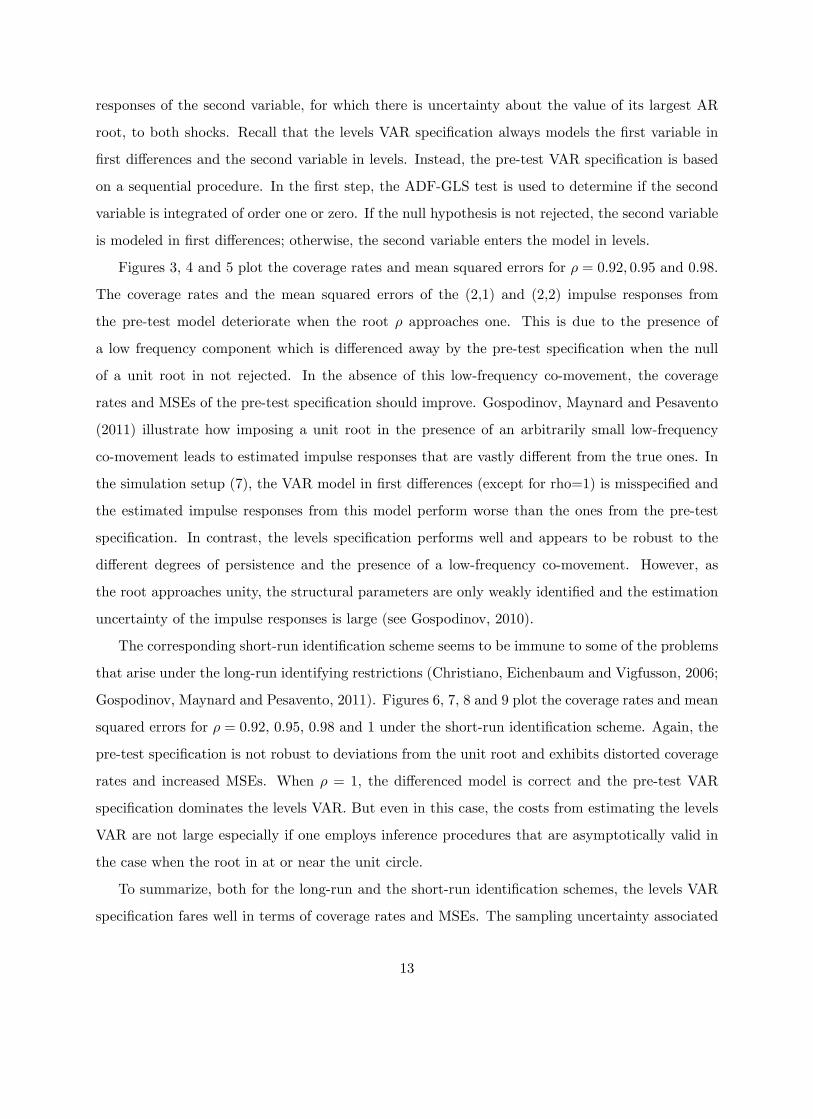
responses of the second variable, for which there is uncertainty about the value of its largest AR
root, to both shocks. Recall that the levels VAR specification always models the first variable in
first differences and the second variable in levels. Instead, the pre-test VAR specification is based
on a sequential procedure. In the first step, the ADF-GLS test is used to determine if the second
variable is integrated of order one or zero. If the null hypothesis is not rejected, the second variable
is modeled in first differences; otherwise, the second variable enters the model in levels.
Figures 3, 4 and 5 plot the coverage rates and mean squared errors for ρ = 0.92, 0.95 and 0.98.
The coverage rates and the mean squared errors of the (2,1) and (2,2) impulse responses from
the pre-test model deteriorate when the root ρ approaches one. This is due to the presence of
a low frequency component which is differenced away by the pre-test specification when the null
of a unit root in not rejected. In the absence of this low-frequency co-movement, the coverage
rates and MSEs of the pre-test specification should improve. Gospodinov, Maynard and Pesavento
(2011) illustrate how imposing a unit root in the presence of an arbitrarily small low-frequency
co-movement leads to estimated impulse responses that are vastly different from the true ones. In
the simulation setup (7), the VAR model in first differences (except for rho=1) is misspecified and
the estimated impulse responses from this model perform worse than the ones from the pre-test
specification. In contrast, the levels specification performs well and appears to be robust to the
different degrees of persistence and the presence of a low-frequency co-movement. However, as
the root approaches unity, the structural parameters are only weakly identified and the estimation
uncertainty of the impulse responses is large (see Gospodinov, 2010).
The corresponding short-run identification scheme seems to be immune to some of the problems
that arise under the long-run identifying restrictions (Christiano, Eichenbaum and Vigfusson, 2006;
Gospodinov, Maynard and Pesavento, 2011). Figures 6, 7, 8 and 9 plot the coverage rates and mean
squared errors for ρ = 0.92, 0.95, 0.98 and 1 under the short-run identification scheme. Again, the
pre-test specification is not robust to deviations from the unit root and exhibits distorted coverage
rates and increased MSEs. When ρ = 1, the differenced model is correct and the pre-test VAR
specification dominates the levels VAR. But even in this case, the costs from estimating the levels
VAR are not large especially if one employs inference procedures that are asymptotically valid in
the case when the root in at or near the unit circle.
To summarize, both for the long-run and the short-run identification schemes, the levels VAR
specification fares well in terms of coverage rates and MSEs. The sampling uncertainty associated
13
with the estimated impulse response functions tends to be well approximated by the bias-corrected
bootstrap procedure of Kilian (1998a,b). The coverage rates and the MSEs of the levels specification
continue to be satisfactory even when the largest root is very close to unity (ρ = 0.95). The
specification based on the pre-test for a unit root exhibits finite-sample distortions and inflated
MSEs. Overall, the levels specification emerges as the preferred specification for this simulation
experiment.
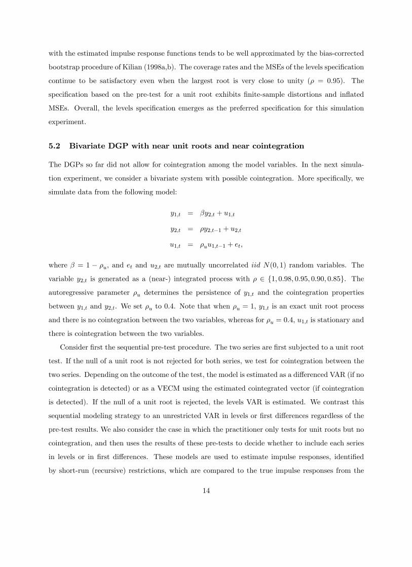
5.2 Bivariate DGP with near unit roots and near cointegration
The DGPs so far did not allow for cointegration among the model variables. In the next simula-
tion experiment, we consider a bivariate system with possible cointegration. More specifically, we
simulate data from the following model:
y1,t = βy2,t + u1,t
y2,t = ρy2,t−1 + u2,t
u1,t = ρuu1,t−1 + et,
where β = 1 − ρu, and et and u2,t are mutually uncorrelated iid N(0, 1) random variables. The
variable y2,t is generated as a (near-) integrated process with ρ ∈ 1, 0.98, 0.95, 0.90, 0.85. The
autoregressive parameter ρu determines the persistence of y1,t and the cointegration properties
between y1,t and y2,t. We set ρu to 0.4. Note that when ρu = 1, y1,t is an exact unit root process
and there is no cointegration between the two variables, whereas for ρu = 0.4, u1,t is stationary and
there is cointegration between the two variables.
Consider first the sequential pre-test procedure. The two series are first subjected to a unit root
test. If the null of a unit root is not rejected for both series, we test for cointegration between the
two series. Depending on the outcome of the test, the model is estimated as a differenced VAR (if no
cointegration is detected) or as a VECM using the estimated cointegrated vector (if cointegration
is detected). If the null of a unit root is rejected, the levels VAR is estimated. We contrast this
sequential modeling strategy to an unrestricted VAR in levels or first differences regardless of the
pre-test results. We also consider the case in which the practitioner only tests for unit roots but no
cointegration, and then uses the results of these pre-tests to decide whether to include each series
in levels or in first differences. These models are used to estimate impulse responses, identified
by short-run (recursive) restrictions, which are compared to the true impulse responses from the
14

model. Unit root pre-tests are performed using the ADF-GLS test at 5% significance level, with
the number of lags chosen by the modified information criterion of Ng and Perron (2001). For the
VAR and VECM estimation we select the number of lags using the BIC (the maximum lag order
is set to 4). We run 10, 000 replications for simulated samples of 200 observations. The results are
presented in Figures 10 to 14.
Figures 10 to 14 show the MSE of the (i, j) impulse response (i = 1, 2; j = 1, 2) for the case in
which there is cointegration in the DGP (ρu = 0.4). Similar to the results in the previous sections,
the levels VAR performs better in terms of MSE than a VAR in first differences except in the case
in which we know for sure that the root is equal to one. Pretesting for a unit root has a similar
effect as in the no-cointegration case: pre-testing provides very little gain when the roots are large
and it is not better than estimating the impulse response from the levels VAR in most cases. For
the (2,1) response, when the root is large, pretesting is actually worse in term of MSE than simply
running the VAR in first differences. As expected as ρ gets smaller, pretests have good power and
they are able to correctly suggest to estimate the VAR in levels.
Comparing the results from estimating a VAR in levels ignoring and not ignoring cointegration
reveals some interesting results: the levels VAR provides a smaller MSE when we pre-test for coin-
tegration even if cointegration is actually present (ρ = 1) for the (1,1) and (2,1) impulse responses.
For the (1,2) and (2,2) impulse responses there is a gain from estimating a VECM when indeed
there is cointegration (ρ = 1). When ρ is less than one, technically there is no cointegration but
we would still expect the variables to behave similarly to the unit root case. For roots as large
at 0.98, and any root smaller than that, the levels VARs performs better for all four impulse re-
sponses. Overall, the results seem to suggest that, in most cases, the levels VAR dominates the
other specifications in terms of MSE although this depends on the impulse responses of interest
and the magnitude of the largest roots in the model.
5.3 A multivariate model used in monetary policy analysis
In the previous section, we considered a bivariate DGP and evaluated the options faced by the
practitioner regarding model specification. When only one unit root is suspected these options
comprise: (a) running a VAR with y2,t in levels ignoring a possible unit root; (b) imposing a unit
root and running a VAR in first differences; or (c) carrying out a pre-test for a unit root in y2,t
and specifying the VAR based on the outcome for the pre-test. Instead, when two unit roots are
15
suspected, the practitioner would be faced with a sequential procedure that could lead to a VAR
model in first-differences, a VECM, a VAR model in levels, or a mixed VAR model with some
variables in levels and some in first-differences.
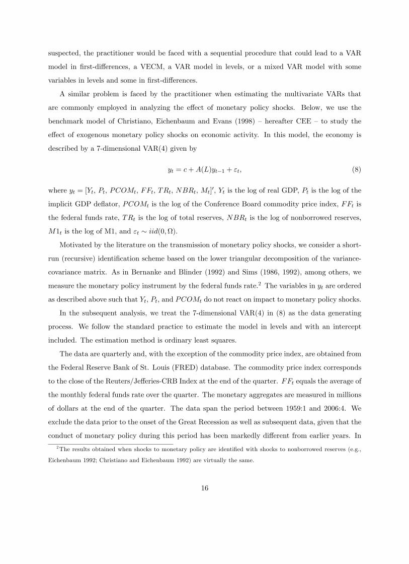
A similar problem is faced by the practitioner when estimating the multivariate VARs that
are commonly employed in analyzing the effect of monetary policy shocks. Below, we use the
benchmark model of Christiano, Eichenbaum and Evans (1998) —hereafter CEE — to study the
effect of exogenous monetary policy shocks on economic activity. In this model, the economy is
described by a 7-dimensional VAR(4) given by
yt = c+A(L)yt−1 + εt, (8)
where yt = [Yt, Pt, PCOMt, FFt, TRt, NBRt, Mt]′, Yt is the log of real GDP, Pt is the log of the
implicit GDP deflator, PCOMt is the log of the Conference Board commodity price index, FFt is
the federal funds rate, TRt is the log of total reserves, NBRt is the log of nonborrowed reserves,
M1t is the log of M1, and εt ∼ iid(0,Ω).
Motivated by the literature on the transmission of monetary policy shocks, we consider a short-
run (recursive) identification scheme based on the lower triangular decomposition of the variance-
covariance matrix. As in Bernanke and Blinder (1992) and Sims (1986, 1992), among others, we
measure the monetary policy instrument by the federal funds rate.2 The variables in yt are ordered
as described above such that Yt, Pt, and PCOMt do not react on impact to monetary policy shocks.
In the subsequent analysis, we treat the 7-dimensional VAR(4) in (8) as the data generating
process. We follow the standard practice to estimate the model in levels and with an intercept
included. The estimation method is ordinary least squares.
The data are quarterly and, with the exception of the commodity price index, are obtained from
the Federal Reserve Bank of St. Louis (FRED) database. The commodity price index corresponds
to the close of the Reuters/Jefferies-CRB Index at the end of the quarter. FFt equals the average of
the monthly federal funds rate over the quarter. The monetary aggregates are measured in millions
of dollars at the end of the quarter. The data span the period between 1959:1 and 2006:4. We
exclude the data prior to the onset of the Great Recession as well as subsequent data, given that the
conduct of monetary policy during this period has been markedly different from earlier years. In
2The results obtained when shocks to monetary policy are identified with shocks to nonborrowed reserves (e.g.,
Eichenbaum 1992; Christiano and Eichenbaum 1992) are virtually the same.
16
particular, nonborrowed reserves took on negative numbers during almost all of 2008 —something
that has never been observed in the documented history of this series —and then increased at a
very fast pace in the following year. Total reserves, on the other hand, exploded during 2008 and
have continued to increase at a very rapid pace. As can be seen in Figure 15, all of the variables
appear to exhibit a high degree of persistence.
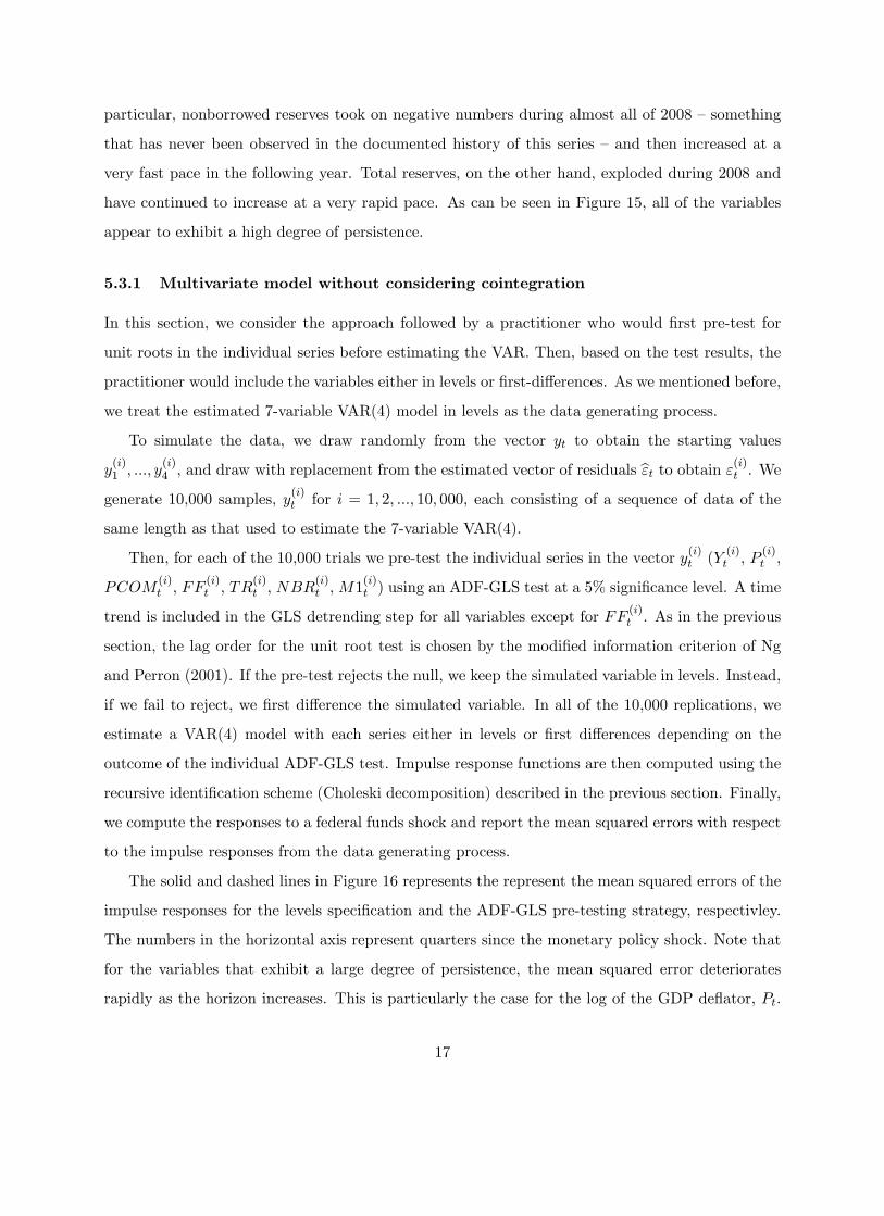
5.3.1 Multivariate model without considering cointegration
In this section, we consider the approach followed by a practitioner who would first pre-test for
unit roots in the individual series before estimating the VAR. Then, based on the test results, the
practitioner would include the variables either in levels or first-differences. As we mentioned before,
we treat the estimated 7-variable VAR(4) model in levels as the data generating process.
To simulate the data, we draw randomly from the vector yt to obtain the starting values
y(i)1 , ..., y
(i)4 , and draw with replacement from the estimated vector of residuals εt to obtain ε
(i)t . We
generate 10,000 samples, y(i)t for i = 1, 2, ..., 10, 000, each consisting of a sequence of data of the
same length as that used to estimate the 7-variable VAR(4).
Then, for each of the 10,000 trials we pre-test the individual series in the vector y(i)t (Y (i)t , P(i)t ,
PCOM(i)t , FF
(i)t , TR
(i)t , NBR
(i)t , M1
(i)t ) using an ADF-GLS test at a 5% significance level. A time
trend is included in the GLS detrending step for all variables except for FF (i)t . As in the previous
section, the lag order for the unit root test is chosen by the modified information criterion of Ng
and Perron (2001). If the pre-test rejects the null, we keep the simulated variable in levels. Instead,
if we fail to reject, we first difference the simulated variable. In all of the 10,000 replications, we
estimate a VAR(4) model with each series either in levels or first differences depending on the
outcome of the individual ADF-GLS test. Impulse response functions are then computed using the
recursive identification scheme (Choleski decomposition) described in the previous section. Finally,
we compute the responses to a federal funds shock and report the mean squared errors with respect
to the impulse responses from the data generating process.
The solid and dashed lines in Figure 16 represents the represent the mean squared errors of the
impulse responses for the levels specification and the ADF-GLS pre-testing strategy, respectivley.
The numbers in the horizontal axis represent quarters since the monetary policy shock. Note that
for the variables that exhibit a large degree of persistence, the mean squared error deteriorates
rapidly as the horizon increases. This is particularly the case for the log of the GDP deflator, Pt.
17
Instead, for the federal funds rate, the MSE increases a quarter after the shock but it drops in the
following quarter staying about the same level in the long-run.
Comparing the lines for the levels specification and the DF-GLS pre-test specification reveals
some intersting results. First, pre-testing for unit roots has the effect of increasing the MSE in
the long-run for all impulse response functions but real GDP. The increase in the MSE, relative
to the levels specification, is larger for the monetary variables, which are characterized by lower
persistence. As it can be seen from the scale of the mean squared errors, the cost associated with
pre-testing for unit roots is not considerably large.3
5.3.2 Multivariate model with possible cointegration
An alternative model selection strategy faced by a practitioner involves considering the possibility
that some of the variables in the system might be cointegrated. In this case, a possible avenue would
be to pre-test for unit roots in each of the series in yt, and then consider cointegration among the
subset of variables that have a unit root. Although this strategy might be employed in practice, the
most commonly used approach is to directly tests for the cointegration rank, without pre-testing
for unit roots. We thus follow the bulk of the literature and address the issue of cointegration in
the full set of variables.
Thus, consider the case where yt might have a VECM representation:
∆yt = Πyt−1 + Γ1∆yt−1 + ...+ Γp−1∆yt−p+1 + ut.
For instance, a number of possible cointegration relationships in a model of monetary transmission is
explored by Juselius (1998a, b). One possibility is that equilibrium in the money market is attained
via stationarity of the liquidity ratio Mt−Pt−Yt, so that a cointegration relationship among these
three variables exists. In addition, inflation and the nominal interest rate could be cointegrated
given the stationarity of the real interest rate. Moreover, the IS relationship would suggest that
trend-adjusted real GDP and inflation (or the interest rate) are cointegrated. Finally, Strongin
(1995) argues that, initially, monetary policy shocks lead only to changes in the composition of total
reserves between borrowed and nonborrowed reserves. Thus, one could conjecture that changes in
3Simulation results (not reported here) suggest that using nonborrowed reserves to identify the monetary policy
shock does not alter our conclusions. In fact, when the data are subject to an ADF-GLS pre-test specification, the
federal funds rate model and the nonborrowed reserves model exhibit mean squared errors of similar magnitudes for
the main variables of interest (i.e., Yt and Pt).
18
the ratio of nonborrowed to total reserves are only short-lived and that a long-run relationship
exists so that TRt and NBRt are cointegrated.
In this section, we evaluate the effect of Johansen’s method (Johansen, 1988) used to pre-test
for the cointegration rank on the MSE of the impulse response functions. In order to do this, we
simulate 10,000 samples of the data generating process as described in the previous section. For
each of these samples, we follow a sequential procedure to determine the cointegrating rank of the
7-variable system (see Lütkepohl 2005, and the references therein). That is, using the trace statistic
we test the sequence of null hypotheses
H0 : rank (Π) = 0;H0 : rank (Π) = 1, ...;H0 : rank (Π) = 6 (9)
and stop the test procedure when the null hypothesis cannot be rejected for the first time. The
cointegrating rank is selected to be the value when the test is stopped. That is, if we cannot reject
the null rank (Π) = 0, the cointegrating rank is taken to be 0 and we estimate a model in first
differences. If the null is rejected, we proceed to test H0 : rank (Π) = 1. This proceeds until we are
not able to reject the null. If the first time we reject the null is for 0 < rank (Π) = r < 7, then the
analysis proceeds with a cointegrating rank of r and a VECM is estimated. Finally, if we cannot
reject the null that rank (Π) = 7, then we estimate a VAR in levels. We use the trace statistic at
5% significance level to test the sequence of null hypothesis describe in (9). The critical values for
the trace test are taken from MacKinnon, Haug and Michelis (1999).
Before we proceed to describe the effects of pre-testing on the impulse response functions, it is
worth mentioning that in 55% percent of the simulations, the trace statistic leads us to conclude
that the rank rank (Π) = 7. Hence, in more than a half of the simulations we use a VAR in levels
when computing the impulse response functions. This result is not surprising because our data
generating process is given by the estimated VAR in levels (equation (8)).
The comparison of the dashed and the dotted lines in Figure 16 suggests some differences in the
MSEs for the impulse responses when we use the ADF-GLS pre-test specification and the Johansen
pre-test specification. Only slight differences are observed in the MSEs on impact and in the short-
run. As the horizon increases, the MSE for the impulse responses of Yt, Pt, TRt, and NBRt are
larger under the Johansen pre-test strategy than if we pre-test for unit roots.
The cost associated with pre-testing for cointegrating rank, as measured by the mean squared
errors, is not large. This finding is consistent with our previous findings based on short-run (recur-
19

sive) identification scheme. Nevertheless, in the long-run, pre-testing for cointegration results in
larger MSEs for all impulse responses —but the log of the GDP deflator—than the levels specification.
6 Concluding Remarks and Practical Recommendations
The practical relevance of structural VARs has been recently questioned (Cooley and Dwyer, 1998;
Chari, Kehoe and McGratten, 2008; among others) with criticisms targeting their theoretical un-
derpinnings, identification assumptions and statistical methodology. Despite these criticisms, the
SVARs prove to be an indispensable tool for policy analysis and evaluation of dynamic economic
models. However, their robustness to uncertainty about the magnitude of the largest roots in
the system and possible co-movements between the variables has not been fully investigated. For
example, the costs from erroneously imposing restrictions (by differencing the data and/or incor-
porating cointegrating relationships) on the models or from estimating unrestricted VAR models
in levels (when the true model is a VECM) have not been quantified for the purpose of impulse re-
sponse analysis under different identification schemes. In this chapter we evaluated the robustness
of alternative VAR specifications to deviations from exact unit roots and cointegration.
The main results and practical recommendations that emerge from our results are the following.
First, under the long-run identification scheme, specification strategies based on pre-tests and
restricted VAR models are not robust to uncertainty about the largest roots of the process and
may lead to highly distorted inference. On the other hand, impulse response estimates from VAR
models using long-run restrictions are inconsistent when the non-unit root variables are expressed
in levels, but have near-unit roots. Thus, applied researchers should exert caution in using models
based on long-run restrictions. We showed that in practice, nevertheless, the VAR specification
with the non-unit root variable in levels is more robust to possible low-frequency co-movements
and departures from exact unit roots.
Second, under the short-run identification scheme, the restricted (based on pre-tests for unit
roots and cointegration) and unrestricted VAR specifications do not exhibit substantial differences
in their computed impulse responses. In other words, the costs from imposing restrictions on the
variables of the model (first differences or cointegration), when these restrictions do not hold exactly
in the true model, do not tend to be too large when the structural impulse responses are identified
through short-run restrictions. However, the unrestricted VAR in levels appears to be the most
20

robust specification when there is uncertainty about the magnitude of the largest roots and the
co-movement between the variables.
We conclude that estimating VAR models in levels and identifying the structural impulse re-
sponses through short-run restrictions emerges as the most reliable strategy for applied work.
21
References
[1] Bernanke, B. S., and A. S. Blinder (1992), “The federal funds rate and the channels of monetary
transmission,”American Economic Review 82, 901—921.
[2] Blanchard, O., and D. Quah (1989), “The dynamic effects of aggregate demand and supply
disturbances,”American Economic Review 79, 655—673.
[3] Chari, V. V., P. J. Kehoe and E. R. McGrattan (2008), “Are structural VARs with long-run
restrictions useful in developing business cycle theory?,”Journal of Monetary Economics 55,
1337—1352.
[4] Christiano, L. J., and M. Eichenbaum (1992), “Identification and the liquidity effect of a mon-
etary policy shock,” in Political Economy, Growth and Business Cycles, eds., A. Cukierman,
Z. Hercowitz, and L. Leiderman, Cambridge and London: MIT Press, 335—370.
[5] Christiano, L. J., M. Eichenbaum and C. Evans (1999), “Monetary policy shocks: What have
we learned and to what end?,” in Handbook of Macroeconomics, Vol. 1A, eds., M. Woodford
and J. Taylor, Amsterdam; New York and Oxford: Elsevier Science, North-Holland.
[6] Christiano, L. J., M. Eichenbaum, and R. Vigfusson (2006), “Assessing structural VARs,”In:
D. Acemoglu, K. Rogoff and M. Woodford, eds., NBER Macroeconomics Annual Cambridge,
MA: MIT Press.
[7] Cooley, T., and M. Dwyer (1998), “Business cycle analysis without much theory: A look at
structural VARs,”Journal of Econometrics 83, 57—88.
[8] Eichenbaum, M. (1992), “Comment on interpreting the macroeconomic time series facts: The
effects of monetary policy,”European Economic Review 36, 1001—1011.
[9] Elliott, G. (1998), “On the robustness of cointegration methods when regressors almost have
unit roots,”Econometrica 66, 149—158.
[10] Gali, J. (1999), “Technology, employment, and the business cycle: Do technology shocks ex-
plain aggregate fluctuations?”American Economic Review 89, 249—271.
[11] Gospodinov, N. (2004), “Asymptotic confidence intervals for impulse responses of near-
integrated processes,”Econometrics Journal 7, 505—527.
22
[12] Gospodinov, N. (2010), “Inference in nearly nonstationary SVAR models with long-run iden-
tifying restrictions,”Journal of Business and Economic Statistics 28, 1—12.
[13] Gospodinov, N., A. Maynard, and E. Pesavento (2011), “Sensitivity of impulse responses
to small low frequency co-movements: Reconciling the evidence on the effects of technology
shocks,”Journal of Business and Economic Statistics 29, 455—467.
[14] Hansen, B. E. (1999), “The grid bootstrap and the autoregressive model,”Review of Economics
and Statistics 81, 594—607.
[15] Hamilton, J. D., and A. M. Herrera (2004), “Oil shocks and aggregate macroeconomic behavior:
The role of monetary policy,”Journal of Money, Credit, and Banking 36, 265—286.
[16] Inoue, A., and L. Kilian (2002), “Bootstrapping autoregressive processes with possible unit
roots,”Econometrica 70, 377—391.
[17] Johansen, S. (1988), “Statistical analysis of cointegration vectors,”Journal of Economic Dy-
namics and Control 12, 231—254.
[18] Juselius, K. (1998a), “A structured VAR for Denmark under changing monetary regimes,”
Journal of Business and Economic Statistics 16, 400—411.
[19] Juselius, K. (1998b), “Changing monetary transmission mechanisms within the EU,”Empirical
Economics 23, 455—481.
[20] Kilian, L. (1998a), “Small-sample confidence intervals for impulse response functions,”Review
of Economics and Statistics 80, 218—230.
[21] Kilian, L. (1998b), “Confidence intervals for impulse responses under departures from normal-
ity,”Econometric Reviews 17, 1—29.
[22] Kilian, L. and P. L. Chang (2000), “How accurate are confidence intervals for impulse responses
in large VAR models?,”Economics Letters 69, 299—307.
[23] Lütkepohl, H. (2005), New Introduction to Multiple Time Series Analysis, Springer-Verlag,
Berlin Heidelberg.
[24] Lütkepohl, H., and H. E. Reimers (1992), “Impulse response analysis of cointegrated systems,”
Journal of Economic Dynamics and Control 16, 53—78.
23

[25] MacKinnon, J. G., A. A. Haug, and L. Michelis (1999), “Numerical distribution functions of
likelihood ratio tests for cointegration,”Journal of Applied Econometrics 14, 563—577.
[26] Mikusheva, A. (2012), “One-dimensional inferences in autoregressive models in a potential
presence of a unit root,”Econometrica 80, 173—212.
[27] Ng, S. and P. Perron (2001), “Lag length selection and the construction of unit root tests with
good size and power,”Econometrica 69, 1519—1554.
[28] Pesavento, E., and B. Rossi (2006), “Small sample confidence intervals for multivariate impulse
response functions at long horizons,”Journal of Applied Econometrics 21, 1135—1155.
[29] Phillips, P. C. B. (1998), “Impulse response and forecast error variance asymptotics in non-
stationary VARs,”Journal of Econometrics 83, 21—56.
[30] Runkle, D. E. (1987), “Vector autoregressions and reality,”Journal of Business and Economic
Statistics 5 , 437—442.
[31] Sims, C. A. (1986), “Are forecasting models usable for policy analysis?,”Federal Reserve Bank
of Minneapolis Quarterly Review 10, 2—16.
[32] Sims, C. A. (1992), “Interpreting the macroeconomic time series facts: The effects of monetary
policy,”European Economic Review, 36, 975—1000.
[33] Sims, C. A., J. H. Stock, and M. W. Watson (1990), “Inference in linear time series with some
unit roots,”Econometrica 58, 113—144.
[34] Stock, J. H. (1991), “Confidence intervals for the largest autoregressive root in U.S. macroeco-
nomic time series,”Journal of Monetary Economics 28, 435—459.
[35] Strongin, S. (1995), “The identification of monetary policy disturbances explaining the liquidity
puzzle,”Journal of Monetary Economics 35, 463—497.
24
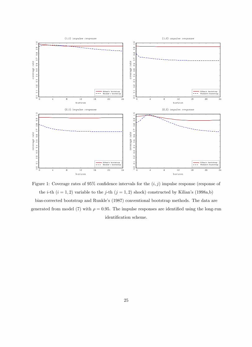
Figure 1: Coverage rates of 95% confidence intervals for the (i, j) impulse response (response of
the i-th (i = 1, 2) variable to the j-th (j = 1, 2) shock) constructed by Kilian’s (1998a,b)
bias-corrected bootstrap and Runkle’s (1987) conventional bootstrap methods. The data are
generated from model (7) with ρ = 0.95. The impulse responses are identified using the long-run
identification scheme.
25
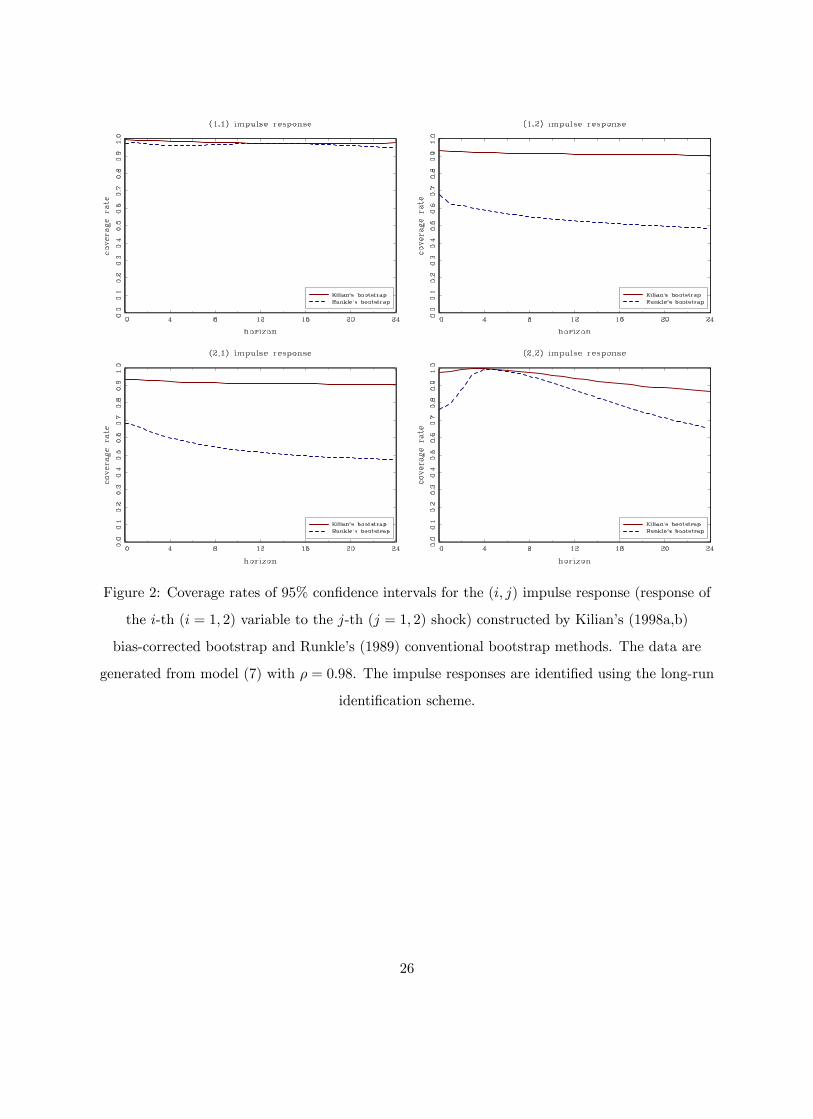
Figure 2: Coverage rates of 95% confidence intervals for the (i, j) impulse response (response of
the i-th (i = 1, 2) variable to the j-th (j = 1, 2) shock) constructed by Kilian’s (1998a,b)
bias-corrected bootstrap and Runkle’s (1989) conventional bootstrap methods. The data are
generated from model (7) with ρ = 0.98. The impulse responses are identified using the long-run
identification scheme.
26
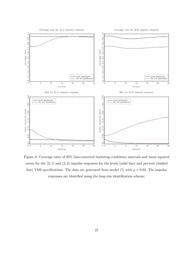
Figure 3: Coverage rates of 95% bias-corrected bootstrap confidence intervals and mean squared
errors for the (2, 1) and (2, 2) impulse responses for the levels (solid line) and pre-test (dashed
line) VAR specifications. The data are generated from model (7) with ρ = 0.92. The impulse
responses are identified using the long-run identification scheme.
27

Figure 4: Coverage rates of 95% bias-corrected bootstrap confidence intervals and mean squared
errors for the (2, 1) and (2, 2) impulse responses for the levels (solid line) and pre-test (dashed
line) VAR specifications. The data are generated from model (7) with ρ = 0.95. The impulse
responses are identified using the long-run identification scheme.
28
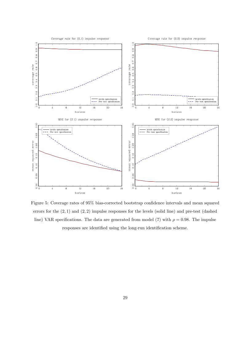
Figure 5: Coverage rates of 95% bias-corrected bootstrap confidence intervals and mean squared
errors for the (2, 1) and (2, 2) impulse responses for the levels (solid line) and pre-test (dashed
line) VAR specifications. The data are generated from model (7) with ρ = 0.98. The impulse
responses are identified using the long-run identification scheme.
29
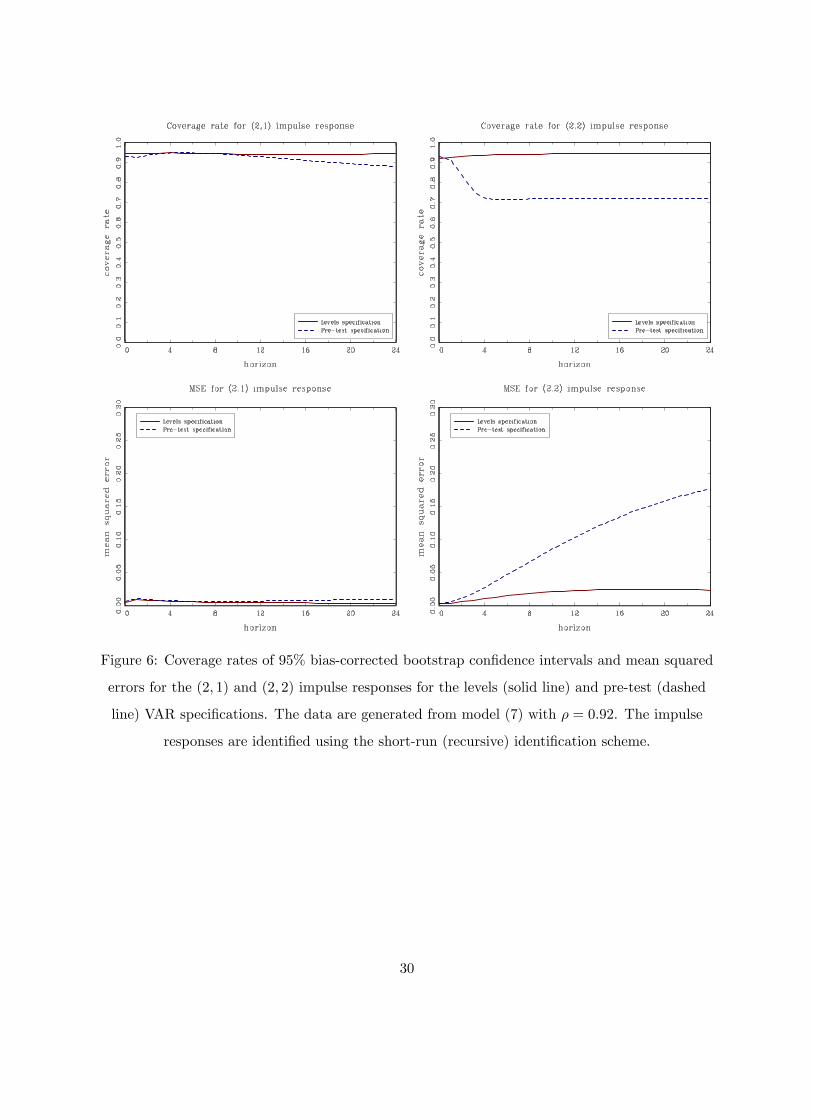
Figure 6: Coverage rates of 95% bias-corrected bootstrap confidence intervals and mean squared
errors for the (2, 1) and (2, 2) impulse responses for the levels (solid line) and pre-test (dashed
line) VAR specifications. The data are generated from model (7) with ρ = 0.92. The impulse
responses are identified using the short-run (recursive) identification scheme.
30
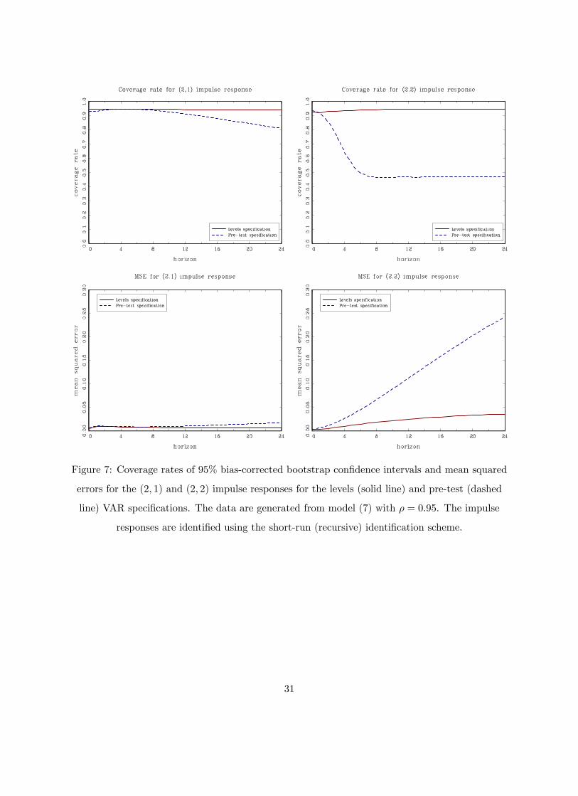
Figure 7: Coverage rates of 95% bias-corrected bootstrap confidence intervals and mean squared
errors for the (2, 1) and (2, 2) impulse responses for the levels (solid line) and pre-test (dashed
line) VAR specifications. The data are generated from model (7) with ρ = 0.95. The impulse
responses are identified using the short-run (recursive) identification scheme.
31
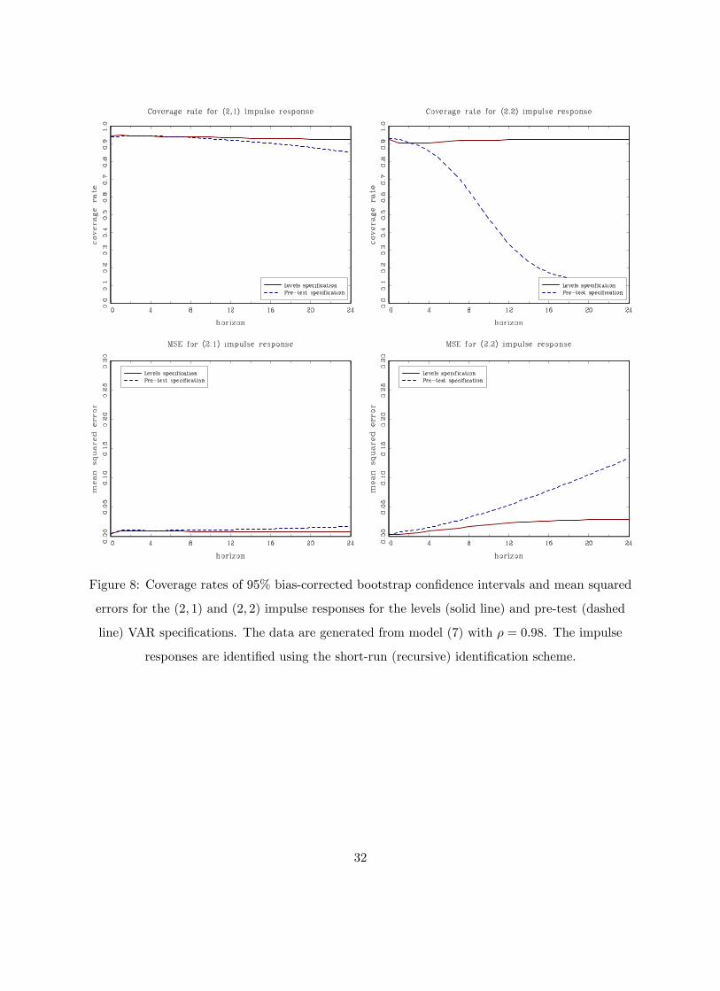
Figure 8: Coverage rates of 95% bias-corrected bootstrap confidence intervals and mean squared
errors for the (2, 1) and (2, 2) impulse responses for the levels (solid line) and pre-test (dashed
line) VAR specifications. The data are generated from model (7) with ρ = 0.98. The impulse
responses are identified using the short-run (recursive) identification scheme.
32
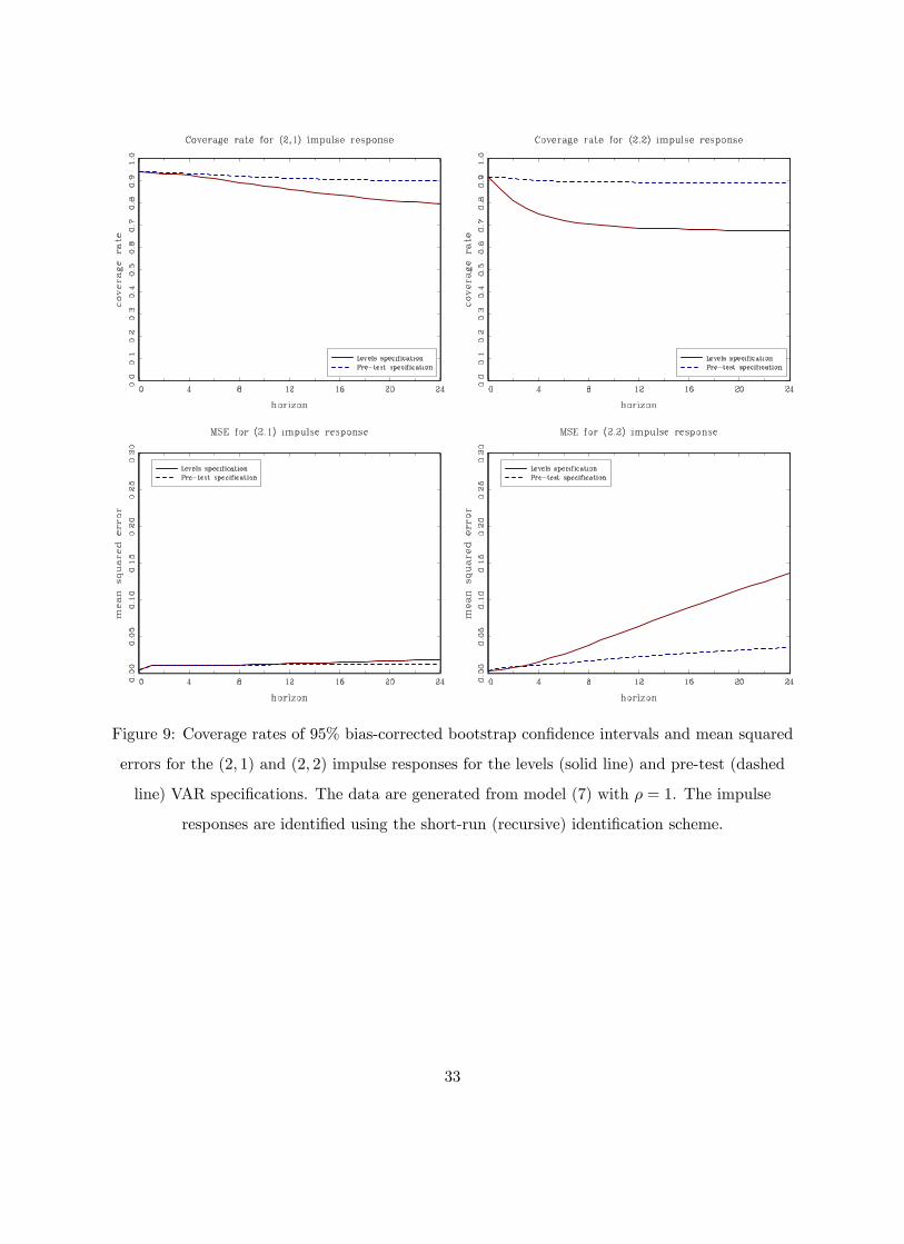
Figure 9: Coverage rates of 95% bias-corrected bootstrap confidence intervals and mean squared
errors for the (2, 1) and (2, 2) impulse responses for the levels (solid line) and pre-test (dashed
line) VAR specifications. The data are generated from model (7) with ρ = 1. The impulse
responses are identified using the short-run (recursive) identification scheme.
33
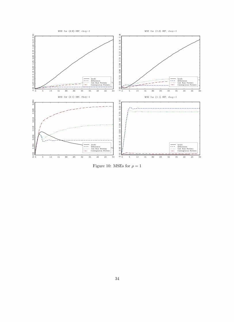
Figure 10: MSEs for ρ = 1
34
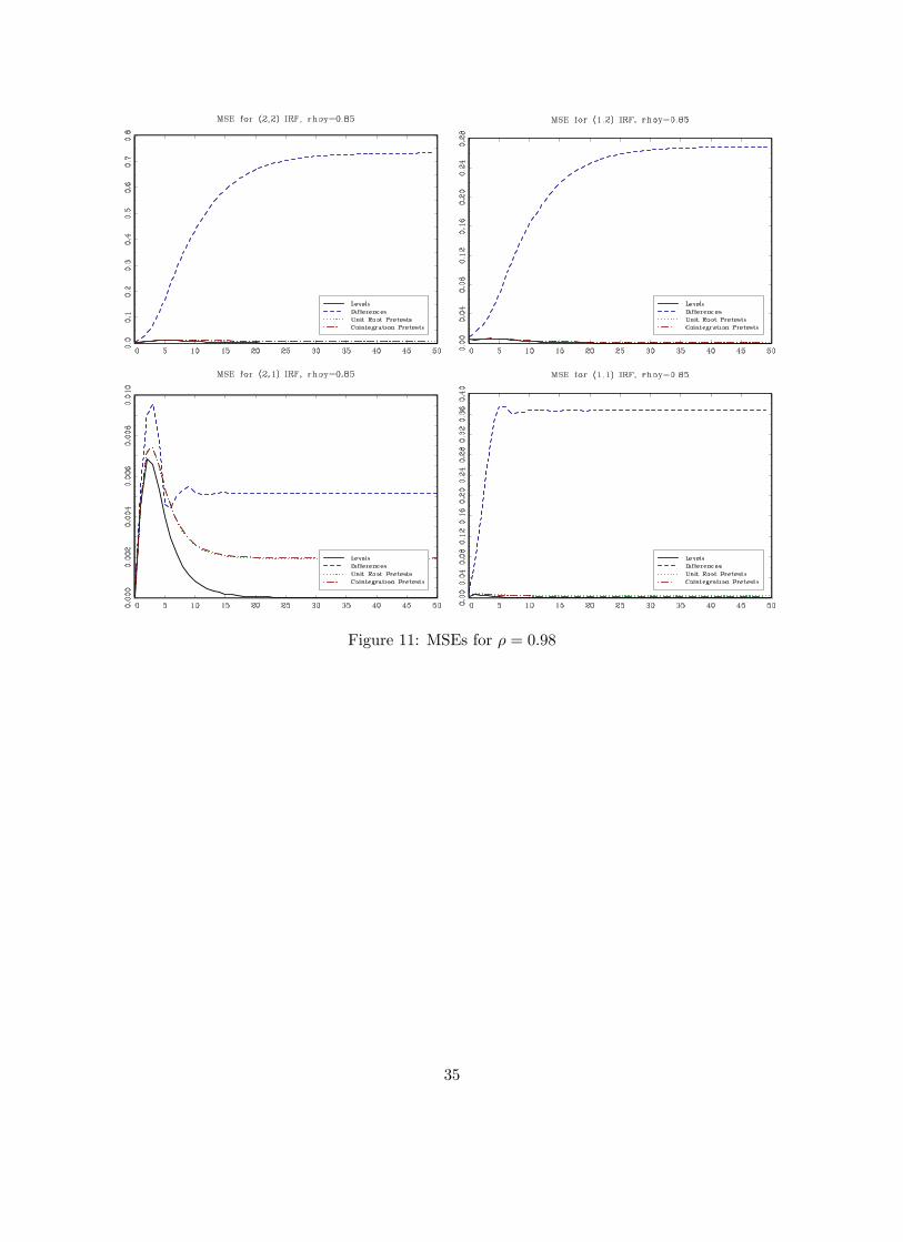
Figure 11: MSEs for ρ = 0.98
35

Figure 12: MSEs for ρ = 0.95
36
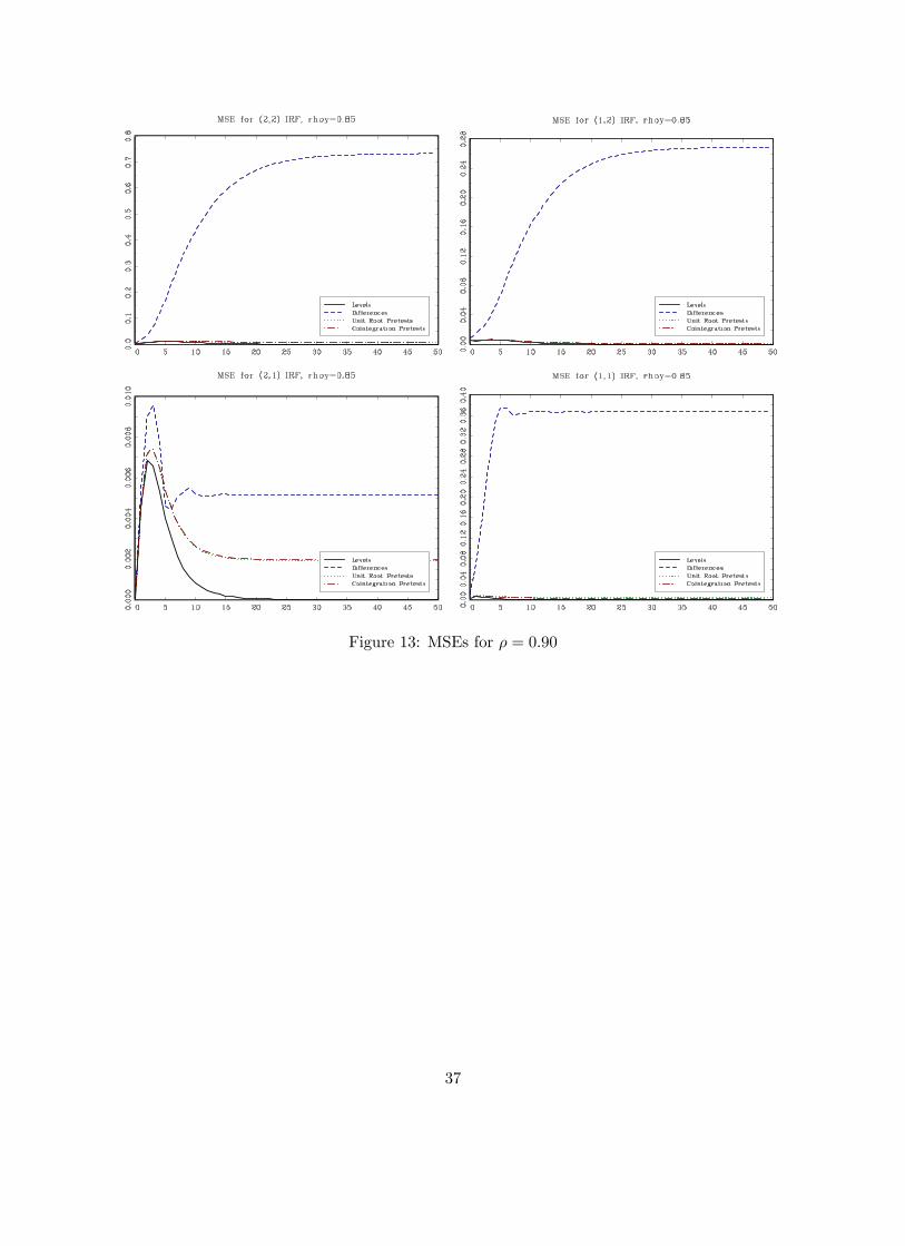
Figure 13: MSEs for ρ = 0.90
37

Figure 14: MSEs for ρ = 0.85
38
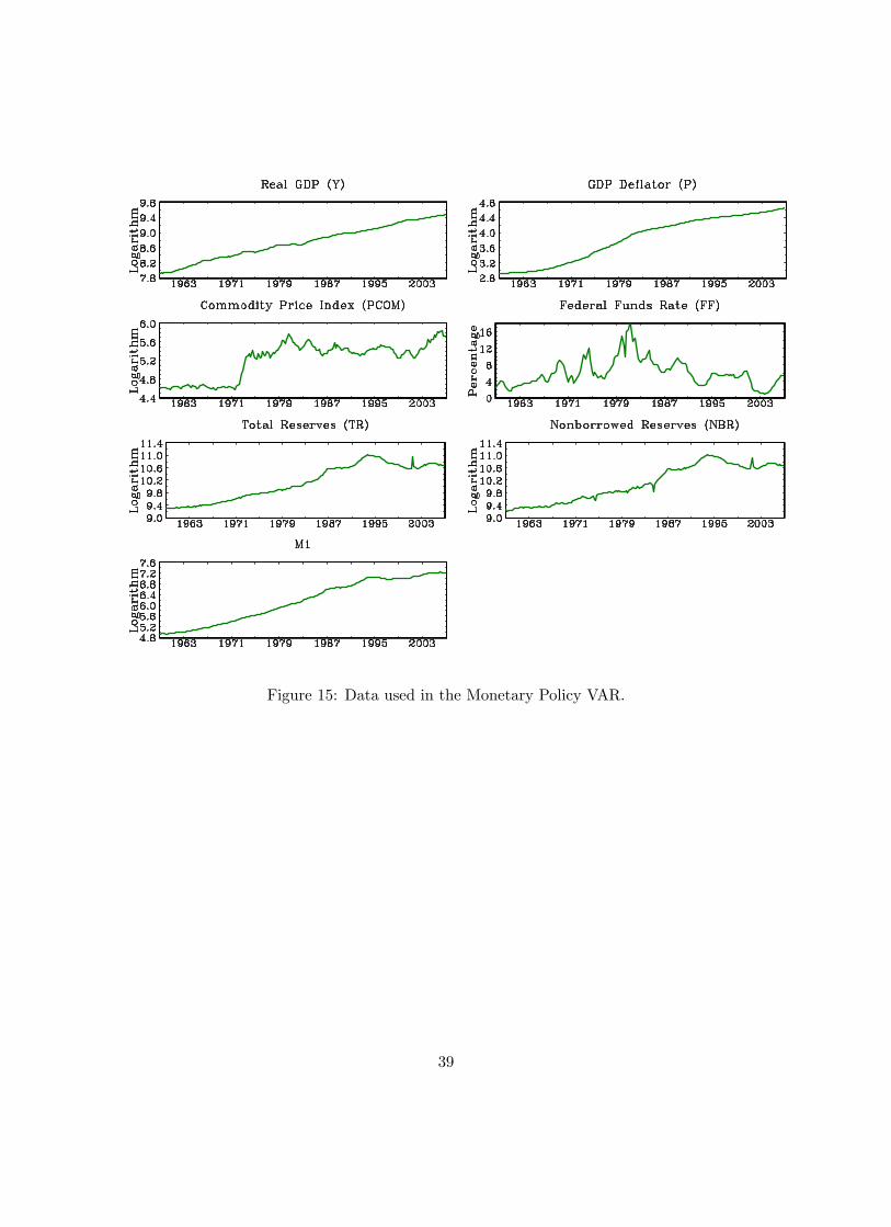
Figure 15: Data used in the Monetary Policy VAR.
39

Figure 16: MSEs for the impulse responses to a federal funds rate shock in CEE model in (8).
The data are generated as described in Section 5.3. The impulse responses are identified using
short-run (recursive) restrictions.
40