UNIVERSITY OF CALIFORNIA Santa Barbara

Economic Feasibility of Seaweed Aquaculture in Southern California

A Group Project submitted in partial satisfaction of the requirements for the degree of Master of Environmental Science and Management

for the Bren School of Environmental Science & Management

by

Ian Ladner Iwen Su

Shaun Wolfe Shelby Oliver

Committee in charge: Hunter Lenihan

May 2018

iii

Table of Contents

Abstract .................................................................................................................................... 1

Executive Summary ................................................................................................................. 2

Candidate species and cultivation methods ............................................................................ 2

Economic feasibility ................................................................................................................ 3

Co-culture with shellfish aquaculture ...................................................................................... 3

Recommendations.................................................................................................................. 3

Background & Project Objectives ........................................................................................... 5

Significance ............................................................................................................................ 5

Seaweed around the globe ..................................................................................................... 5

Seaweed in the United States ................................................................................................ 6

Seaweed in California ............................................................................................................. 6

Potential for seaweed in the Southern California Bight ........................................................... 7

Environmental benefits and challenges .................................................................................. 8

Project objectives ................................................................................................................... 9

1. Identification of candidate species and cultivation methods ..........................................10

Introduction ...........................................................................................................................10

Methods ................................................................................................................................11

Finding suitable seaweeds for cultivation in the Southern California Bight .........................11

Determining optimal conditions and growth rates ...............................................................12

Results and Analysis .............................................................................................................13

Finding suitable seaweeds for cultivation in the Southern California Bight .........................13

Determining optimal conditions and growth rates ...............................................................16

Discussion .............................................................................................................................21

Limitations to growth rate estimates ...................................................................................21

Conclusion ............................................................................................................................22

2. Feasibility of seaweed aquaculture in southern California ..............................................23

Introduction ...........................................................................................................................23

Methods ................................................................................................................................24

Model inputs ......................................................................................................................24

Model outputs ....................................................................................................................27

iv

Results and Analysis .............................................................................................................28

Break-even price point at year five .....................................................................................28

Onshore versus offshore cultivation methods .....................................................................29

Species variability in costs .................................................................................................33

Assessing the seaweed market opportunities ....................................................................34

Model sensitivity to changes in growth rate, risk and market price .....................................36

Discussion .............................................................................................................................37

Onshore vs offshore ...........................................................................................................37

Effect of permitting on feasibility .........................................................................................38

Opportunities to reduce capital and operating costs for seaweed aquaculture ...................39

Conclusion ............................................................................................................................40

3. Integrating seaweed into an existing mussel farm ...........................................................41

Introduction ...........................................................................................................................41

3.1 Economically optimal mussel-seaweed farm ..................................................................42

Methods ................................................................................................................................42

Calculating profit per unit of production for M. galloprovincialis ..........................................43

Estimating demand curve for edible seaweed ....................................................................43

Calculating profit per unit of production for G. pacifica .......................................................44

Results and Analysis .............................................................................................................46

Discussion .............................................................................................................................48

3.2 Offshore field experiment .................................................................................................49

Methods ................................................................................................................................49

Study site ...........................................................................................................................49

Mussel growth and condition index ....................................................................................49

Seaweed growth study .......................................................................................................50

Statistical analysis ..............................................................................................................50

Results ..................................................................................................................................50

Mussel growth (length) .......................................................................................................50

Mussel quality (condition index) .........................................................................................52

Seaweed Growth ...............................................................................................................53

Discussion .............................................................................................................................54

Conclusion ............................................................................................................................55

v

4. Concluding remarks and recommendations .....................................................................56

Cultivation techniques ........................................................................................................56

Marketing ...........................................................................................................................57

Political Atmosphere ..........................................................................................................57

Outlook ..............................................................................................................................58

References ..............................................................................................................................59

Appendices .............................................................................................................................69

Appendix A: Biology and life-cycle of seaweed ......................................................................69

Appendix B: Hydrographic conditions at our farm location in Santa Barbara, CA ...................72

Appendix C: Seaweed data ...................................................................................................72

Appendix D: Seaweed yield summary ...................................................................................78

Appendix E. Cost information ................................................................................................79

Appendix F. Cash flow analyses (cont.) .................................................................................87

vi

Acknowledgements

This report was made possible by the combined knowledge and support of a whole host of

people. We would specifically like to thank the following individuals for their contributions to this

project:

Bernard Friedman, Client, Santa Barbara Mariculture

Hunter Lenihan, Faculty Advisor, Bren School

Jessica Couture, PhD Advisor, Bren School

Phoebe Racine, Project Coordinator, Sustainable Aquaculture Research Center

Doug Bush, External Advisor, The Cultured Abalone Farm

Norah Eddy, External Advisor, Salty Girl Seafood

Daniel Marquez, Owner, PharmerSea

Heidi Herrmann, Owner, Strong Arm Farms

Michael Graham, Owner, Monterey Bay Seaweeds

Michael Friedlander, Scientific Advisor, Seakura

Randy Lovell, Aquaculture Coordinator, CA Department of Fish and Wildlife

John Corbin, President, Aquaculture Planning and Advocacy LLC

Peter Fischer, Owner, Maine Fresh Sea Farms

J. Robert Waaland, Professor Emeritus, University of Washington

Bren School: Andrew Plantinga, Professor; Chris Costello, Professor; Olivier Deschenes,

Professor; Gonzalo Banda-Cruz, Master’s Candidate

UC Santa Barbara: Daniel Reed, Professor; Sutara Nitenson, Intern; Ellen Hollstien, Intern

1

Abstract Global aquaculture production of seaweed is a staggering 23.8 million tonnes per year, with a net worth of $6.4 billion USD. The majority of edible seaweeds consumed in California is imported from Asia and local seaweed product is overwhelmingly sourced from wild harvesters in northern California. Reliance on imports and wild harvesting can have large environmental consequences and put additional pressure on regional marine ecosystems. As the demand for local seaweed in California increases interest has grown in developing a seaweed aquaculture industry through both onshore and offshore systems. However, the technical and economic feasibility of growing native California seaweed species as local alternatives to the major imported species — nori, kombu, and wakame— has not been assessed. Our project investigated which seaweed species have the most potential based on market demand and suitability to local environmental conditions. We identified four promising candidates in the Southern California Bight and the appropriate methods for their cultivation. We then developed a bioeconomic model to highlight the key factors that determine the economic feasibility of establishing a seaweed aquaculture industry in the region. Finally, we undertook a preliminary assessment of seaweed integration into an existing local mussel farm. Our results show that regional seaweed aquaculture is economically feasible, that there are important considerations for siting production on or offshore, and that co-culturing seaweed with shellfish can provide a jumpstart to the industry as a whole. These findings provide stakeholders and policymakers a blueprint for prioritizing next steps in expanding sustainable seaweed aquaculture in southern California.

2

Executive Summary

Seaweed aquaculture is an emerging industry in the United States, but has been established in many Asian countries for centuries. Over one-fifth of global annual aquaculture production comes from seaweed, with the vast majority of that being used for direct human consumption (Moffit, 2014). Seaweed is produced for a wide variety of uses, including pharmaceuticals, biofuel, and agricultural products, but food and health are human necessities that may motivate the more rapid expansion of local, sustainable aquaculture. The rich nutritional profile and low environmental footprint of seaweed contribute to its promise as a sustainable and healthy food source. To date, increasing demand for edible seaweeds in California has been primarily filled by imported products (NOAA Fisheries, 2017). However, the environmental and oceanographic conditions of California’s waters are an untapped resource for seaweed cultivation as evidenced by the dense stands of kelp forest along the coast. The lack of need for freshwater and pesticide inputs makes seaweed aquaculture a prime candidate to sustainably address food security issues in California.

In our project, we focused on seaweed species that satisfy a growing health-conscious community and have a high potential in the southern California food market. We assessed the economic feasibility of starting a seaweed farm in onshore (i.e. land-based) and offshore. Here, offshore is defined as mariculture occurring in ocean but does not necessarily refer to cultivation in deep and distant waters. The main barriers impeding the growth of the industry are high initial capital costs, permitting uncertainty, and a lack of established cultivation methods specific to the region. Our report aims to provide researchers, future farmers, and policy makers comprehensive scientific knowledge about ideal candidate species for edible seaweed cultivation, prospective economic feasibility, and mechanisms to circumvent some of those barriers in the short term.

Candidate species and cultivation methods

We utilized three criteria to identify edible seaweed species that are ideal for cultivation and sale in southern California: 1) The algae must occur naturally throughout the whole region, 2) have a pre-existing food market in California, and 3) must have established aquaculture techniques. The first condition helps promote a cohesive and collaborative local industry and the latter two are desirable by aquaculturists who want to buy into a system that has a proven history of success. Applying these criteria to the native species of the Bight, the following four species emerge as the most promising candidates:

Gracilaria pacifica (ogo or limu) - a delicate red seaweed used as a topping for poke and rice bowls

Pyropia perforata (nori) - a local variant of a highly marketable red genus that is commonly dried for sushi rolls

Ulva lactuca (sea lettuce) - a productive green species found in soups and seaweed salads

Laminaria setchellii (kombu) - a sturdy brown seaweed that is sought after for use in soup stock or consumed whole

Optimal harvest season and potential productivity for a locale can be estimated by using knowledge of species physiological tolerance ranges and a combination of ambient

3

environmental conditions, such as water temperature, nutrient availability, and photoperiod. The final decision facing a farmer is which grow-out structure to use for a particular species. All four aforementioned species can be grown in tanks onshore. For offshore cultivation, longline culture is most appropriate for G. pacifica and L. setchellii, whereas P. perforata and U. lactuca should be raised used nets. Since the latter two species are more susceptible to rough wave action, siting them in calmer or shallower waters will decrease the likelihood of fragmentation.

Economic feasibility

We synthesized projected farm yield, initial required capital, and annual operating costs through a bioeconomic model to investigate the key factors that will affect the economic feasibility of seaweed aquaculture in southern California. Seaweed growth rate has a major influence on the viability of a farm system and L. setchellii outperformed the other three candidate species largely due to its high biological productivity and low annual harvest costs. However, as a brown seaweed, it typically has a lower market value than a red species such as P. perforata. This suggests potential trade-offs in species selection between productivity and marketability. Our research also highlights the pros and cons of siting seaweed production on and offshore. Offshore production can be more economically viable due to its lower annual operational costs, but a farmer may be forced to make sacrifices in terms of product quality and increased risk. Additionally, securing a permit for offshore aquaculture has proven to be more difficult than for onshore systems. An aquaculture farmer can have more control over product quality onshore but this comes at the price of higher labor and energy costs. Our models predicts an average price of $11.42/kg across the four species for an onshore farmer to recoup their costs over a five-year time period compared to $6.84/kg offshore. Regardless of location, these “break-even” prices suggest that the cost of seaweed aquaculture in southern California prohibits successful competition on the global market, where seaweed is processed for use as a food additive. Instead, the seaweed industry must position itself to provide a value-added produce or specialty item to be viable.

Co-culture with shellfish aquaculture

In California and elsewhere around the globe, seaweed aquaculture has been increasingly associated with shellfish cultivation. These two extractive organisms have been traditionally paired with fed finfish aquaculture, a process known as integrated multitrophic aquaculture (IMTA). However, shellfish and seaweed can also be grown together in isolation. Shellfish farmers benefit from diversifying their product portfolio and potential seaweed farmers can leverage existing permits for shellfish aquaculture to avoid having to obtain a new one. Sharing required infrastructure and novel “3-D” cultivation methods allows for increased yield from a single farm unit. This project demonstrates that an existing mussel farm could increase its profit by substituting seaweed production on to the farm. It is also possible that there are ecological benefits of growing the two species in unison, such as localized buffering of ocean acidification by seaweeds, but further empirical research is needed to corroborate these theories.

Recommendations

Seaweed aquaculture can be economically feasible in southern California but barriers exist that prevent the development of a regional industry. We recommend stakeholders should focus their efforts on adapting current cultivation techniques for use in California waters, identifying the most effective marketing strategies, and creating a political framework in support of sustainable

4

best management practices. Future steps will include validating the growth rate estimates utilized in this report and quantifying the health and environmental benefits of seaweed aquaculture for consumers and decision makers. Further research should investigate co-culture with shellfish and the polyculture of multiple seaweed species to maximize economic and biological outcomes. Through increased collaboration between researchers, policy makers, and aquaculture farmers, sustainable seaweed aquaculture can be the next innovation in California’s rich history of food production.

5

Background & Project Objectives

Significance

Aquaculture is poised to help address food security issues as the world’s population continues

to grow (FAO, 2014). A shift towards more domestic production in the United States would allow

for the creation of many jobs and stricter control of the sustainability and environmental impact

of the industry. While finfish and shellfish aquaculture have received significant attention in the

academic and political realms, the cultivation of edible seaweeds is a relatively novel idea

throughout much of the U.S. coastal zone. Seaweeds, or macroscopic algae, are nutrient rich,

require very few inputs (including no freshwater), and thrive in the upwelling zone along the

coast of the western United States. These facets make the production of seaweed for direct

human food use appealing to consumers, policy makers, and aquaculturists alike.

Interest in seaweed aquaculture is growing here in southern California, but many questions

remain as to the feasibility of the industry. To our knowledge, there has been no assessment of

the economic feasibility of growing native California seaweed species for food use. Additionally,

no review has summarized which native seaweed species to target, what cultivation methods

are most appropriate, and the limitations and uncertainties regarding seaweed aquaculture in

California. Our project seeks to address these questions and provide a framework for future

studies to build upon when assessing the economic feasibility of seaweed in California and

other regions. Additionally, identifying the most ideal seaweed candidates will help direct future

research toward these species.

Seaweed around the globe

23.8 million tonnes of seaweed are produced globally every year, valued at $6.4 billion USD (Moffitt, 2014). Over 95% of seaweed products are farmed, accounting for over a fifth of global annual aquaculture production (Moffitt, 2014). Out of the 33 countries that harvest seaweed, China is the largest producer by a significant margin with limited production in Western countries. Cultivation of seaweed grew 50% globally between 2004 and 2014 (Nayar & Bott, 2014). However, the demand for it is still outpacing supply as the global seaweed market doubled from 2000 to 2012 (West et al., 2016). Out of all groups cultivated, the market for red seaweeds is growing the most rapidly at 8% annually (West et al., 2016). Seaweed produced for human consumption as fresh, dried, or processed products makes up 80% of the value of the global market while the remainder is mainly used in pharmaceuticals, agricultural fertilizer, and aquaculture feed (Buchholz et al., 2012; McHugh, 2003; Nayar & Bott, 2014; West et al., 2016). Algal hydrocolloids, such as carrageenan and agar, are used as emulsifying, gelling, or water retention agents. However, sustainable food production is a popular topic with which more people can engage compared to seaweed cultivation for alternative energy use or high-end cosmetics that are non-essential. In the international edible seaweed market, the most dominant species are the red seaweeds Kappaphycus alvarezii and Eucheuma spp., which are used to produce carrageenan (Moffitt, 2014). These are followed by seaweeds consumed dried or raw, such as Laminaria japonica (kombu or Japanese kelp),

6

Gracilaria spp. (ogo, limu), Undaria pinnatifida (wakame) and Pyropia spp. (nori). Pyropia (formerly referred to as Porphyra) is by far the most valuable seaweed species with two species, P. yezoenisis and P. tenera, constituting the bulk of global production (Jensen, 1996; Levine & Sahoo, 2009). Numerous health benefits are attributed to seaweed including high levels of iodine, fiber, and trace minerals, although nutrient contents vary greatly across species (Fleurence, 1999; MacArtain et al., 2007). For example, the calcium concentration in some seaweeds exceeds that of whole milk, making it particularly attractive for use in health food or vegan products (MacArtain et al., 2007). Given the health benefits associated with consuming seaweed, tremendous growth potential exists for this product in health-conscious markets within the US, Canada, and Europe.

Seaweed in the United States

The supply of farmed, wild harvested, and imported seaweed has grown over the past decades in the United States as the American palate begins to accept and integrate seaweed. Seaweed imports increased 65% from 1999 to 2008 (Nayar & Bott, 2012). In 2016, the U.S. imported over 31 metric tons of seaweed, a 19.7% increase from 2015 (NOAA, 2017). This seaweed was valued at about $146 million USD (NOAA, 2017). Most edible seaweed production occurs on the east coast and in Hawai’i, largely through the harvest of Chondrus crispus (irish moss) and Palmaria palmata (dulse). More recently, aquaculturists have begun cultivating Saccharina latissima (sugar kelp) and Gracilaria spp (ogo or limu) as well. There is also an increasing effort in the US to move towards an ecosystem-based approach known as integrated multi-trophic aquaculture (IMTA), a technique that harnesses the benefits of culturing two or more species from different trophic levels together. Rapid increase in demand for seaweed products is expected to continue domestically due to the potential for a new, sustainable, and healthy protein source (Buck et al., 2017). This has already been seen in Maine where seaweed sales doubled every year for the first 6 years of seaweed aquaculture production, between 2009-2015 (Lem, 2016). The easiest market entry point for seaweed domestically is in high-end restaurants. Chefs are drawn by its rich nutrition profile and are experimenting with it at increasing rates (Mouritsen, 2012). Out of the most commonly consumed species, Pyropia spp. and Palmaria palmata have been identified as having the highest protein quantity and quality respectively (Holdt and Kraan, 2011). Despite varying substantially across species, the nutritional aspect of seaweed is crucial to its potential marketability (MacArtain et al., 2007; McHugh, 2003).

Seaweed in California

Despite limited seaweed aquaculture research and development in California, seaweed harvest is growing rapidly. In 2004, harvested seaweed amounted to over 33,000 metric tons, making it the 5th most landed taxon by weight on the west coast (Norman et al., 2007). As of 2014, harvesting of kelp (Macrocystis pyrifera) has declined rapidly, while edible seaweed harvest (e.g. species from Pyropia, Laminaria, and Monostrema) has increased (CDFW, 2014). The seaweed harvest occurs primarily in northern California, with many commercial harvesters operating in Mendocino County and near San Francisco (e.g. Strong Arm Farms in Sonoma,

7

Mendocino Sea Vegetable Company and Rising Tide Sea Vegetables in Mendocino). There are strict harvesting regulations including permitted areas, protected species, and limits on the annual harvest quantities. Commonly hand harvested seaweed species in California are Macrocystis pyrifera (giant kelp), Nereocystis luetkeana (bull kelp), Mastocarpus papillatus (turkish washcloth), Laminaria setchellii (kombu) and Stephanocystis osmundacea (bladder chain kelp) (CDFW, 2014). While coastal seaweed aquaculture has developed to varying extents on the eastern seaboard and in Hawai’i, businesses and stakeholders are just starting to consider growing seaweed off the coast of California. Currently, no ocean farmed seaweed exists in California. Suitable local seaweed species, methods for culturing them in the eastern Pacific Ocean, and the economic feasibility of farm methods still need to be identified. Therefore, seaweed aquaculture remains limited in California, with the only existing production occurring in tanks on land. The three current land based seaweed farms in California are: Monterey Bay Seaweeds in Moss Landing, Carlsbad Aquafarm in Carlsbad, and The Cultured Abalone Farm in Santa Barbara. The farms in Santa Barbara and Carlsbad primarily grow shellfish but augment their operations with production of Gracilaria pacifica. Meanwhile, Monterey Bay Seaweed grows Palmaria palmata (Northeast Atlantic dulse), Gracilaria spp., and Ulva spp in recirculating tanks as its sole products. In Santa Barbara, G. pacifica is used for abalone and fish feed, and sold to restaurants and food processors. Monterey Bay Seaweeds sells to chefs and high-end restaurants in the wider Monterey Bay Area (e.g. San Francisco, Santa Cruz), and these seaweeds are processed live and transported in saline water to their destination. The existing seaweed market can provide useful insight into potential seaweed candidates, target markets, and ways to add value through processing.

Potential for seaweed in the Southern California Bight

Nutrient-rich, upwelled waters off the southern California coast provide a unique opportunity to cultivate seaweed with minimal inputs (Sautter & Thunell, 1991). These are the same waters that support the algae-dominated kelp forest ecosystems that line the region’s coastline (Brzezinski et al., 2013). The environmental conditions of the Southern California Bight, the coastline between Point Conception and San Diego, also cater to the strict light and temperature requirements that many cultivated seaweeds have. Water temperatures and photoperiods in the region are relatively homogenous year-round (Appendix B). In addition to physical and chemical ocean properties, the Southern California Bight is also an epicenter for the health-conscious food market in the United States (Guthman, 2004). Having immediate access to the target market will likely lead to more economic success for the seaweed aquaculture industry (D. Bush, pers comm, 2018; M. Graham, pers comm, 2018).

Despite the numerous promising characteristics of the Southern California Bight for seaweed

aquaculture, the industry remains underdeveloped. Part of the current dialogue in the industry

focuses on the decision to site production onshore or offshore. Delicate species that are likely to

fragment benefit from the less dynamic conditions when cultured on land (M. Graham, pers

comm). Onshore farms are much easier to get permitted but are typically more energy intensive

and expensive to operate (D. Bush, pers comm, B. Friedman, pers comm, 2017; Huguenin,

1976;). Open-ocean farms could be a good alternative to land-based systems since there are

few inputs in the form of energy, seawater intake, and added nutrients (Nobre et al 2010).

8

However, open-ocean farms don’t come without challenges in California. Spatial conflicts with

other ocean users such as the Navy, commercial fishers, and tourism operations exist, but could

be minimized with careful planning (Gentry et al., 2017). Understanding the tradeoffs between

onshore and offshore may enable decision makers to make more informed choices regarding

future seaweed aquaculture development along the Southern California Bight.

Environmental benefits and challenges

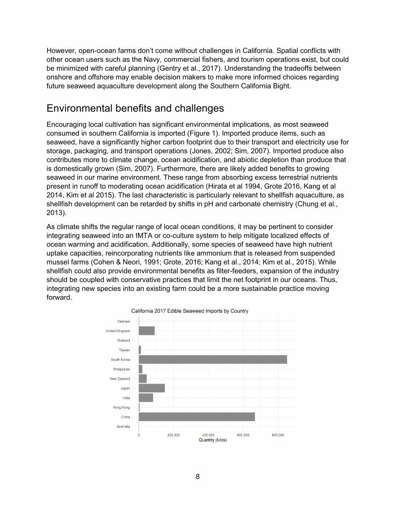
Encouraging local cultivation has significant environmental implications, as most seaweed

consumed in southern California is imported (Figure 1). Imported produce items, such as

seaweed, have a significantly higher carbon footprint due to their transport and electricity use for

storage, packaging, and transport operations (Jones, 2002; Sim, 2007). Imported produce also

contributes more to climate change, ocean acidification, and abiotic depletion than produce that

is domestically grown (Sim, 2007). Furthermore, there are likely added benefits to growing

seaweed in our marine environment. These range from absorbing excess terrestrial nutrients

present in runoff to moderating ocean acidification (Hirata et al 1994, Grote 2016, Kang et al

2014, Kim et al 2015). The last characteristic is particularly relevant to shellfish aquaculture, as

shellfish development can be retarded by shifts in pH and carbonate chemistry (Chung et al.,

2013).

As climate shifts the regular range of local ocean conditions, it may be pertinent to consider

integrating seaweed into an IMTA or co-culture system to help mitigate localized effects of

ocean warming and acidification. Additionally, some species of seaweed have high nutrient

uptake capacities, reincorporating nutrients like ammonium that is released from suspended

mussel farms (Cohen & Neori, 1991; Grote, 2016; Kang et al., 2014; Kim et al., 2015). While

shellfish could also provide environmental benefits as filter-feeders, expansion of the industry

should be coupled with conservative practices that limit the net footprint in our oceans. Thus,

integrating new species into an existing farm could be a more sustainable practice moving

forward.

9

Figure 1. Edible seaweed imports to California in 2017 by country. Total imports by weight is 1,926,273

kg valued at an average of $13.38/kg. Source: NOAA Fisheries, Fisheries Statistics Division: Commercial

Fisheries Statistics, 2017 Cumulative Trade Data by U.S. Customs District.

In general, concerns still persist regarding the greater aquaculture industry like escape, benthic

and aquatic pollution from waste and excess feed, and use of antibiotics that may create drug-

resistant parasites and bacteria. However, many of these do not apply to properly managed

seaweed aquaculture (Costa-Pierce, 2002). Cultivating native species greatly reduces the

ecological impacts of escape. Seaweeds are net nutrient sinks which limits their environmental

footprint and makes them valuable in IMTA systems (Troell et al., 2009). Finally, no pesticide or

freshwater inputs are required to grow seaweed in the Southern California Bight. This is

particularly important given the region’s limited water resources and frequent bouts with drought

(MacDonald, 2007).

There are still concerns about local seaweed aquaculture offshore in addition to the spatial

issues outlined in the previous section. The most unrelenting concern is marine mammal

entanglement (R. Lovell, pers comm, 2017). There have been 5 reported cases globally of turtle

and cetacean entanglement in offshore mussel farm equipment, which is structurally similar to

seaweed aquaculture equipment (Young, 2015). Although entanglement is suspected to be

underreported, 5 occurrences in the last two decades suggest fairly small risk (Lindell and

Bailey, 2015). Moreover, the risk of marine mammal aquaculture entanglement is significantly

less than that of traditional fishing gear (Young, 2015).

Project objectives

Perhaps the greatest challenge to growing seaweed in the Southern California Bight is that

interested parties simply don’t have the framework for a successful seaweed aquaculture

operation in the region. While more information is available for onshore farming, questions

remain for both onshore and offshore systems about what species to grow, when and where to

grow those species, what cultivation method to use, and how profitable these operations could

be. Because seaweed aquaculture in the Southern California Bight promises less risk, fewer

environmental threats, and more environmental benefits than traditional terrestrial agriculture

and other forms of aquaculture, there is growing interest both onshore and offshore from groups

like Ventura Shellfish Enterprise, the Port of San Diego, and Catalina Sea Ranch. Our project

completed a comprehensive analysis of the ideal candidate species with regards to the

requirements for their cultivation and the relative economic feasibility of doing so. To accomplish

this, we set out the following project objectives:

1) Identify southern California candidate seaweed species and the appropriate cultivation

methods

2) Determine key factors that influence economic feasibility in each species-farm system

through the use of a bioeconomic model

3) Perform a preliminary investigation of incorporating seaweed into an existing mussel

farm

10

Through the first objective, we selected the most promising species from those native to the

Southern California Bight using a mixed criteria of technical ease and market suitability. In the

next section, we projected the economic feasibility of the seaweed aquaculture industry in the

region via a synthesis of estimated farm costs and annual biological yield. We also outlined the

variables and processes that stakeholders should focus on to improve business sustainability.

Finally, we examined the benefits to both industries of integrating seaweed cultivation into

existing mussel aquaculture through our partnership with Santa Barbara Mariculture, an open-

ocean mussel farm off the coast of Hope Ranch.

1. Identification of candidate species and

cultivation methods

Introduction

A major challenge for seaweed aquaculture in the Southern California Bight is the lack of

research and development done on native seaweeds for aquaculture in the region (see

Background). Seaweed farming is a multi-stage process that is shaped by the life-history and

ocean condition preferences of the target species. These two factors greatly influence the

cultivation methods used and the respective costs (Pereira & Yarish, 2008). Before establishing

a seaweed farm, a farmer must decide 1) where to place the farm (onshore or offshore), 2)

which species to grow, 3) the best method and timing for cultivating the species, and 4) the

economic feasibility of these decisions (Radulovich et al., 2015; Titlyanov & Titlayanova, 2010).

In this chapter, we describe the decisions facing a potential seaweed farm, steps that must be

taken at the various phases, and provide the best available data to inform the first three

questions above.

Farm location and which species to produce are the first decisions that must be evaluated by an

interested aquaculturist. For intensive seaweed farming, the two possible locations are onshore

or in the ocean (i.e. offshore). Onshore pertains to seaweed cultivated on-land and includes

pond and tank culture; offshore is used to describe any operation where seaweed is grown in

the ocean, regardless of the proximity of the farm to the shore (McHugh, 2003). As discussed in

the Background, onshore production offers benefits in the way of permitting ease and risk

reduction for fragile species that may fragment (M. Graham, pers comm, 2017). Conversely,

offshore farms are typically cheaper to operate and are less energy intensive, but the lack of

control over environmental conditions often results in highly variable annual production

(Huguenin, 1976).

The life history, ocean condition preferences, locality of species, cultivation potential, and

marketability all have to be considered when selecting a seaweed species to cultivate

(Radulovich et al., 2015). Interested farmers are unlikely to choose a species that isn’t cultivated

globally (B. Friedman, pers comm, 2017). Farms should only consider seaweeds native to the

region to avoid the risk of introducing a foreign species. Selecting a native seaweed species

also provides confirmation that the species can grow in that region for at least part of the year. It

is important to compare the optimal environmental conditions for each species to those

observed in the farms locale to ensure that the seaweed will have the appropriate levels of light,

11

nutrients, temperature, and other environmental variables (Santelices, 1999). Furthermore, the

local oceanographic regime can influence the chosen seaweed’s reproductive schedule which

will have a significant impact on farm operations. The reproductive schedule directly limits the

growth and harvest seasons of some species of seaweed (Titlyanov & Titlyanova, 2010). Some

species have complicated life cycles that require land-based hatchery facilities that can carefully

control water temperature, nutrients, and light (McHugh, 2003). Hatcheries are the sites at

which reproduction is induced to seed the production units that will later be placed offshore.

Seaweeds are grouped into three taxonomic clades: red (Rhodophyta), green (Chlorophyta),

and brown (Phaeophyta). Each group has unique differences in reproductive and life-history

modes (Appendix A). The wide variety of reproductive, physiological, and morphological forms

amongst seaweeds results in highly specialized cultivation strategies that must be determined

for each species. Broadly, there are four major steps in the cultivation of macroalgae: 1)

hatchery phase, 2) nursery phase, 3) grow-out phase, and 4) harvest phase but not all species

require each of these phases.

Once a farmer has chosen a species of seaweed to grow, they must select a growing method.

Broadly, several methods of offshore cultivation exist including: fixed pole, semi floating raft,

floating raft, open water ropes, nearshore ropes, baskets, and nets (Kim et al., 2017). Some

taxa have multiple applicable cultivation methods while others are typically only grown using

one structure (Kim et al., 2017). The most common cultivation methods onshore are growing

seaweed in tanks or ponds (Kim et al., 2017; McHugh, 2013). These various cultivation methods

depend on farm location and incur vastly different costs depending on the species and locale.

After life history, cultivation potential, and ocean conditions are accounted for, marketability

needs to be considered. The chosen species must have a proven market for increased chance

of success. While many markets for seaweed exist and have been discussed throughout this

paper, we have chosen to focus on the direct for human consumption market. The majority of

the value global seaweed aquaculture is in the food market and local farmers can tap into its

higher price point to increase their economic viability (D. Bush, pers comm, 2018; M. Graham,

pers comm, 2017; McHugh, 2003). The entire evaluation process from site location to

marketability is outlined in further detail in the methods section of this chapter.

Methods

To determine ideal candidate species, their optimal cultivation structures, and their theoretical

growth rates in the Southern California Bight, we used the following six procedures: 1) identify

species that occur throughout the Southern California Bight, have a food market, and are from a

taxa widely cultivated in aquaculture systems, 2) determine the ideal grow-out structures both

on and offshore, 3) establish oceanographic conditions at our model site, 4) match these

conditions with the ambient environmental requirements for the seaweed species, 5) determine

the best cultivation schedule regarding hatchery, out-planting, and harvesting, and 6) ascertain

high and low growth rates for the seaweed species in offshore and onshore regions.

Finding suitable seaweeds for cultivation in the Southern California Bight

We first identified all seaweed taxa that grow throughout the full range of the Southern California

Bight using the Jepson Herbarium at the University of California, Berkeley, which resulted in 191

12

genera of species (UC Berkeley, n.d.). We only used species that occur throughout the entire

Southern California Bight since the growth rates for species reaching their thermal limits will be

limited, and thus, not appropriate for mass cultivation. Furthermore, using seaweed that grows

outside of its native range raises concerns with introducing a foreign species. Based on these

criteria, we excluded six seaweed species that have been found at only at the very northern

range of the Southern California Bight (Santa Barbara County) and in low densities. This

included the following species: Postelsia palmaeformus, Palmaria mollis, Alaria marginata,

Gigartina papillata, and Fucus gardneri. Next, we cross-referenced this list with the genera that

have a direct human consumption/food market in Southern California (Abbott & Hollenberg,

1992; Kim et al., 2017; Titlyanov & Titlyanova, 2010). Finally, we eliminated any species which

are not grown in aquaculture systems globally (McHugh, 2013; Titlyanov & Titlyanova, 2010).

For the remaining candidate species, we conducted a literature review and spoke with industry

experts to determine the appropriate grow-out structures (e.g. nets, tanks) needed for each

species in offshore and onshore regions in the Southern California Bight.

Determining optimal conditions and growth rates

Seaweed species growth rates in offshore regions are highly dependent on oceanographic conditions. Thus, it is necessary to time ideal growth conditions with the offshore outplanting/cultivation period of the seaweed species. We reviewed the literature to identify what environmental settings our seaweed candidates prefer and compared those against historical ocean conditions recorded by NOAA, SCCOOS, UC Santa Barbara LTER, and CalCOFI for our chosen farm location at Santa Barbara Mariculture in Santa Barbara, CA (Appendix B). The exact coordinates for the study are as follows: 34°23'39.2"N 119°45'09.8"W. We chose this location because it is the only permitted and functioning offshore aquaculture farm of any type in the region. However, Santa Barbara Mariculture grows shellfish and does not currently grow seaweed.

After matching optimal seaweed growth conditions to the seasonality of those factors at our study site, we compared the potential growing season to how the life cycle of the seaweed affects harvest and may be affected by ocean conditions. We were then left with an optimal growing and harvest season. For onshore, the ocean temperature remained an important factor in determining seasonality but nutrient levels were not as important since farmers can easily manipulate these by adding fertilizer to their system.

Once we established what to grow, how to grow it, and when to grow it, we had to estimate the growth rate and annual yield for each candidate species. The following methodology was used to select growth rates:

1. Determined monthly (Jan-Dec) values of temperature, dissolved inorganic nitrogen, current speed, photoperiod, and irradiance in regions representative of our client’s farm location. Sources: SCCOOS, CalCOFI Stations, UC Santa Barbara (UCSB) LTER, and NOAA reports of historic values.

2. Collected discrete daily relative growth rates for a specific set of environmental conditions from various seaweed culture experiments, culture handbooks, and publications.

3. Where species specific data were lacking, we used morphologically, genetically, or reproductively similar species as a proxy for the local Southern California Bight species.

13

4. Selected the stocking density most commonly used in literature or one that led to optimal growth in the absence of a ubiquitous value.

5. Chose the growth rates or growth rate range that best matches the environmental system in the Southern California Bight and our understanding of the biology of our local species. At times, an estimated or measured final yield at the end of each harvest period (e.g. 7 kg per meter of longline) as a more reliable indicator of potential productivity.

6. Selected a representative high and low growth rate if there were clear peak and slow periods/months during a single harvest season or a single year. We did not include a requirement that these two were sourced from the same study for every species.

7. When peak and slow periods for our local species were not available, we used algal abundance studies (e.g. UCSB LTER) to approximate which months out of the year we were likely to see the species grow its best.

Results and Analysis

Finding suitable seaweeds for cultivation in the Southern California Bight

We identified nine species that are extant throughout the entire Southern California Bight and

are sold for direct human consumption (Table 1.1). From these nine species, we excluded those

that do not have a food market in California or are not from genera with established aquaculture

practices. This resulted in our four candidate species that we used for further analysis regarding

their economic feasibility in southern California. Below, we present information on our candidate

species and the other five species that were excluded from our study.

Table 1.1. The nine seaweed species that were considered for their potential in seaweed aquaculture in

the Southern California Bight. The final four candidate species and five excluded species, along with the

justification for exclusion, are shown.

14

Candidate species

Gracilaria pacifica

Gracilaria pacifica, or “ogo”, is grown in

aquaculture systems, occurs from Santa

Barbara to San Diego (and beyond), and has a

food market (Abbott & Hollenberg, 1992; D.

Bush, pers comm, 2018; Kim et al., 2017). It is

generally consumed fresh as a topping for poke

bowls or dried and processed for use as a rice

seasoning. This species is grown onshore in

tank culture in southern California currently and

can be cultivated offshore on ropes, cage-like

structures, and on the nearshore benthos (Kim

et al., 2017; Yarish et al., 2012).

Pyropia perforata

This species grows naturally between San Diego and

Santa Barbara (Abbott & Hollenberg, 1992). The genus

Pyropia (previously Porphyra) has a large and

extremely valuable food market and aquaculture

industry globally, including on the west coast of the

United States (Kim et al., 2017; Levine & Sahoo, 2010;

Sindermann, 1982). P. perforata is hand harvested,

dried, and then sold by commercial harvesters in

Northern California (e.g. Mendocino Sea Vegetables;

Rising Tide Sea Vegetables), and has been grown in

aquaculture system experimentally (Waaland, 1977). Commonly known as “nori”, P. perforata is

often dried and processed into thin sheets for sushi rolls. We selected P. perforata as a

candidate species due to its potential value and the wide cultivation of its genus. Pyropia spp.

are commonly grown on nets via fixed pole, semi floating rafts or floating rafts offshore (Figure

1.2; Kim et al., 2017; Levine & Sahoo, 2009).

Ulva lactuca

Both species of Ulva common in California are

found in our range (Abbott & Hollenberg, 1992).

Ulva lactuca is grown in aquaculture systems and

has a food market (M Friedlander, pers comm,

2018; Titlyanov & Titlyanova, 2010). “Sea lettuce”

is frequently utilized fresh in seaweed salads and

soups. Ulva lactuca are generally grown on nets

offshore or in tank cultures onshore (Brandenburg,

2016; Cohen and Neori, 1991).

Figure 1.2. Fixed pole net cultivation of Pyropia (McHugh, 2013).

Figure 1.1. Tank cultivation of G. pacifica (Mazza, 2017).

Figure 1.3. U. lactuca in the wild (Peters, 2006).

15

Laminaria setchellii

Laminaria spp. are grown commercially in aquaculture

systems, occur in our range, and have a food market

(Abbott & Hollenberg, 1992; Mendocino Sea

Vegetables; Rising Tide Sea Vegetables; Titlyanov &

Titlyanova, 2010). Therefore, we chose to consider L.

setchellii as a native representative of this genus.

While this species is not currently consumed by

humans, other Laminariales, or “kombu”, are a staple

product in Asian cuisines and are consumed raw,

cooked, and dried. Laminaria spp. are grown on

longlines or lines via floating rafts offshore and in

tanks onshore (Figure 1.4; McHugh, 2013; Peteiro et

al., 2006, Titlyanov & Titlyanova, 2010).

Species that do not meet all criteria

Chondracanthus exasperatus

Chondracanthus exasperatus grows in our target region and is being/has been grown on a

small scale in Washington (Waaland, 2004). The market for this species exists solely in the

cosmetic industry and thus did not fit our criteria for having a food market in the U.S. (Boratyn,

2000; Lewallen & Lewallen, 1996; Waaland, 2004).

Eisenia arborea

This species grows in Santa Barbara and has been identified as having potential for commercial

cultivation (Abbott & Hollenberg, 1992; Zertuche-Gonzalez et al., 2016). However, the food

market for this species is very small and primarily exists in Asia (Zertuche-Gonzalez et al.,

2016).There is no evidence of a U.S. market. Furthermore, it is not currently cultivated in

aquaculture systems and there is generally a lack of information on this species outside of wild

harvesting it for abalone feed or experimenting with it in powder form to treat allergies

(Zertuche-Gonzalez et al., 2016). The lack of a current food market and the lack of information

for the commercial cultivation of this species caused us to eliminate it from consideration.

Gelidium robustum and Gelidium spp.

G. robustum grows throughout our target region and is most productive in nutrient rich,

upwelling regions (Abbott & Hollenberg, 1992; Santelices, 1991). There are potentially small

food markets in China and Japan for Gelidium spp (Doty et al., 1987; FAO, 1994; Fotedar &

Phillips 2011; Salinas, 1991). However, the cultivation of Gelidium spp. is still experimental and

not currently seen as economically viable (Cremades, 2012; Doty et al., 1987; Fotedar &

Phillips, 2011; Salinas, 1991). Given the lack of established wide-scale cultivation practices, we

excluded Gelidium spp.

Figure 1.4. A kelp species grown on longlines as Laminaria setchellii would be (The

Seaweed Site, 2018)

16

Agardhiella coulteri

This species occurs within the Southern California Bight range but there is no evidence of a

direct human consumption market (Abbott & Hollenberg, 1992). Other seaweeds in the

Agardhiella genus are cultivated for their phycocolloids and are starting to be used for shellfish

feed (Garr et al., 2009; Chopin et al., 1989; Huang & Rorrer, 2002).

Hypnea spp.

Hypnea spp. grow in the northern end of the Southern California Bight (i.e. Santa Barbara

County), but are extremely rare (Jepson Herbarium, 2018). The genus is commercially

cultivated, but there is no evidence of a food market and is typically processed as a phycocolloid

(Wallner et al., 1992; Ding et al., 2013; Ganesan et al., 2005). Given that Hypnea does not grow

throughout our entire study range, it was excluded.

Determining optimal conditions and growth rates

With our list of candidate species finalized, we identified ideal environmental conditions, growth

rates, and the seasonality of the grow-out and harvest periods for each species in both an

onshore and offshore system. When data for our candidate species in our region was not

available, we tried to use data from studies done with synonymous species (in regard to life

cycle and morphology) at similar latitudes with similar ocean current patterns. All final

parameters discussed in this section are summarized in Appendix C.

Gracilaria pacifica

Most of the studies found in literature for offshore Gracilaria growth were performed on other

species (i.e. G. gracilis) or had non-nutrient limiting environments (concentrations of NO3-

between 15.3 and 33.5 uM). Maximum growth rates reported were as high as 11% (Davison,

2015; Wakibia et al., 2011). However, these rates would most likely be limited by nutrient

availability in the Santa Barbara Channel. To estimate growth at our client’s farm off Hope

Ranch, Santa Barbara, we used a two-week field growth study that was conducted by the

Sustainable Aquaculture Research Center (SARC) onsite in March 2016 for Gracilaria pacifica.

It is likely that March falls during the most productive time of year for G. pacifica due to the

nutrient concentrations being the highest around this time, according to historic trends from

UCSB LTER and CalCOFI monitoring data.

From our research, we predicted that G. pacifica growth is most influenced by light and nutrient

availability. This high value taken from the SARC experiment for relative growth rate was 3.98%

per day (Table 1.2). The low growth rate is taken from the Halling et al. (2005) study that grew

Gracilaria chilensis offshore in Chile. While this is not a perfect replicate of Santa Barbara, both

locations have Mediterranean climates with equatorial currents (pole to equator, colder waters).

We set the lower end of our growth range at 1.44% (Table 1.2), a value that was one standard

deviation lower than the mean reported in that study. The stocking density (0.4 kg/m) was taken

from Dawes (1995), which produced similar growth rates to that in the SARC experiment.

17

Table 1.2. Low and high growth rates for candidate species both offshore and onshore. In some

instances, the most reliable growth estimate found in the literature was a final annual production instead

of daily relative growth rate. These are indicated as such below and the equivalent relative growth rate

was calculated for use in our bioeconomic model.

Species Offshore Growth Onshore Growth Data Sources

Gracilaria

pacifica 1.4 - 3.98% RGR per day 5.48 – 6.9% RGR per day SARC, Halling et al 2005; SARC

Ulva spp. 3.3 – 6.67 kg/m2 annual production 10 – 17.6% RGR per day

Titlyanov & Titlyanova 2010;

Duke et al 1989; Hernandez et

al 2005

Pyropia

perforata 2.96 - 6.52 kg/m2 annual production 10 – 16% RGR per day

Parker 1974, Miura 1975; Kim

et al 2007

Laminaria

spp. 7 – 16 kg/m annual production 0.85 – 1.3 % RGR per day

Peteiro & Freire 2013, Watson

& Dring 2013; Azevedo et al

2016

G. pacifica may have a slower growing period for months December - February and in June

given the nutrient concentration in Santa Barbara. As a peak growing season was available in

the literature for the Southern California Bight, we relied on a combination of expert opinion,

oceanographic monitoring data, and abundance estimates of native Gracilaria spp. in the area

(D. Reed, pers comm, 2018; UCSB LTER). Gracilaria pacifica naturally occurs on Mohawk Reef

near the Santa Barbara Harbor between the months of March and October with a peak between

May and July (SB LTER). There are fairly low amounts of DIN (NO3, NO2, NH3) between July

and November (< 1.2 uM), which start to drop in June to 2 uM (UCSB LTER). The longest

photoperiod is from March to October (UCSB LTER). Therefore, it is likely that G. pacifica is

nutrient limited in the summer and limited by light availability in the winter time (Santelices,

1999).We found one case in Chile where Gracilaria is cultivated every 7 months, but here we

use the average cultivation period of 6 months (Winberg, 2011). We determined that G.

pacifica’s ideal harvest period would likely be March through June at a minimum, but extended it

through August to obtain a six month cultivation season (Figure 1.5).

Data for onshore G. pacifica growth rates was sourced directly from a local aquaculture farm in

Santa Barbara. Stocking density and growth rate were both taken from a SARC pilot growth

study conducted onshore in Goleta, California during late summer and early fall of 2017 (J.

Couture, pers comm, 2018). We used 6.9% and 5.48% as the high and low daily relative growth

rate from that study. Stocking density associated with the reported growth was 3.17 kg/m3.

Based on prior experience, G. pacifica has the ability to grow year round January to December

in an onshore tank system (D. Bush, pers comm, 2018). We set a weekly harvest frequency (D.

Bush, pers comm, 2018; Davison & Piedrahita, 2015).

18

Figure 1.5. Onshore and offshore cultivation timelines for the four candidate species.

Ulva lactuca

Ulva lactuca is initially cultivated by allowing its spores to settle out onto nets, and we assumed

an initial stocking density of 0.25 kg per m2. Then we used a final reported yield of 0.5 – 1.0 kg

dry weight per m2 (Titlaynov & Titlyanova, 2010). Using an average conversion factor from

literature of 6.67 kg wet weight to 1 kg dry weight, we determined the high and low wet weight

yield to be 6.67 kg per m2 and 3.3 kg per m2 respectively (Azevedo et al., 2016; Hernandez et

al., 2005; Roesijadi et al., 2008; Watson & Dring, 2007). From there, we back calculated the low

and peak growth rates to be 2.6% and 4.96% per m2 per day. While these growth rates from

Titlaynov and Titlaynova (2010) were lower than other growth rates reported, the high growth

rates observed in other studies were instantaneous and recorded only for a short period of time.

We determined the thermal optimum for Ulva lactuca to take place from May to October given

the North Sea range of 15-20 °C (Figure 1.5). During this time, temperatures in Santa Barbara

are over 15 °C and photoperiod is also the highest (between 13.97 and 11.33 hours). U. lactuca

reproduces from June-August, but the reproductive phase occurs for only a short period during

peak season and doesn't affect the harvest (M. Freidlander, pers comm, 2018). Natural

abundances in Santa Barbara are generally highest around spring and summer (D. Reed, pers

comm, 2018). Ulva can survive in low nutrient ranges as long as the temperature is below 20

°C, as is the case at our farm location (Duke et al., 1989). Therefore, we expect U. lactuca to

still grow well during summer despite lower nutrient levels.

There were several onshore Ulva spp. studies available for U. curvata and U. lactuca, many of

which reported extremely high growth rates. The estimates range from 10 and 65% relative

19

growth per day (Carl et al., 2014; Duke et al., 1989; Neori et al., 1991). In a constrained system,

such as a tank or a densely packed offshore farm, density-dependent factors slow down growth

or cause mortality (Neori et al., 1991). The low growth rate of 10% per day is a reasonable

expectation, but we had to limit the high growth rate based on our physical farm constraints.

First, harvest frequencies reported for Ulva spp. in onshore systems were in the range of 3-4

weeks, so we used an average of 3.5 weeks (M. Friedlander, pers comm, 2018; van den burg et

al., 2012). Then, the initial (0.375 kg/m3) and maximum (27.8 kg/m3) stocking density were used

to calculate the maximum growth rate over a single harvest period (Duke et al., 1989;

Hernandez et al., 2005). The calculated high growth rate was 17.6% per day, which falls in the

range of growth reported in literature. Similar to G. pacifica, Ulva spp. can persist vegetatively

for at least a year from the same source, so stocking can occur yearly (Bolton et al., 2009; M.

Friedlander, pers comm, 2018).

Pyropia perforata

We used a final yield value of 1100 sheets per net (18m x 1.5m net size) for our high growth

estimate using a conversion factor of 25 sheets per 1kg of fresh Pyropia perforata (Levine &

Sahoo, 2009; Parker, 1974). We assumed that four nets were seeded and deployed during the

annual growing period (KMO, 1982). Yield values for Pyropia spp. vary greatly, but 1100 sheets

per net is well within the lower production ranges found in literature. Given that Pyropia spp. has

to be seeded on nets in a hatchery, stocking densities aren’t relevant or reported. In order to

calculate a growth rate, we needed a stocking density and assumed a value of 1kg/m2. The

average harvest period for Pyropia spp. is 37.5 days (Kim et al., 2017; Levine and Sahoo,

2009). We had to back-calculate a growth rate given these parameters to yield 1100 sheets per

net. Our final value was 3.2% per day per m2. For our low growth rate, we completed the same

calculation but used a very conservative final yield of 500 sheets per net and calculated growth

to be 1.05% per day per m2 (Miura, 1975).

Through our literature review, we were not able to elucidate the nutrient requirements for P.

perforata. P. perforata can withstand extremely high levels of nutrients, but there is no mention

in any study of the minimum required nutrient input (Romero, 2009). At the genus level, Pyropia

spp. prefer 100-200 mg/m3 of nitrogen for optimal growth, which is within the 43-200 mg/m3

available at the farm site in Santa Barbara (Chen & Xu, 2005). Light is overwhelmingly the most

important factor for P. perforata growth and 8-16 hours of light per day is optimal for all Pyropia

spp (Pereira, 2006). Multiple studies suggest that 10-20 °C is the optimal temperature for

Pyropia spp (Kim et al., 2007; Pereira et al., 2006). There is no optimal temperature

estimated/recorded specifically for P. perforata.

Wild populations of P. perforata are most abundant in mid spring to early fall, however this is not

the best harvest season for the species (Romero, 2009). Pyropia perforata releases

carpospores when photoperiods exceed 12 hours at low temperatures coinciding with upwelling

periods (Pacheco-Ruiz et al., 2005). Photoperiods in Santa Barbara exceed 12 hours between

April and September, upwelling occurs between March and May, and temperatures are lower in

the spring (Brzezinski et al., 2013). Thus, sporing will likely begin in the spring and harvest

should be completed around then to avoid allocation of metabolic energy to reproduction.

Nutrients are lowest between July and November, so there is concern that Pyropia may not

grow well during this period (Appendix A). We chose to set that harvest period as the harvest

period of December to April as the best balance between all the environmental factors. This

time period is colder in temperature, avoids photoperiods over 12 hours, and takes advantage of

20

the upwelling and higher nutrient availability. This is when Pyropia spp. are grown in Japan, but

Japanese Pyropia spp. prefer cold water and ocean conditions are more variable in the Western

Pacific (MacFarlane, 1966).

Onshore, we used the high and low relative growth rates of 16% and 10% per day per m3 from

the only study to conduct research on four species of Pyropia in land-based tanks (Kim et al.,

2007). Other studies have reported significantly higher relative growth rates than were stated in

in the Kim et al. (2007) study. However, this may be due to the fact that the other experiments

used younger seaweed blades (< 10 cm) that uptake nutrients faster and grow more rapidly

(Kim et al., 2007). The initial stocking density we used was from an onshore culture experiment

in Israel (Israel et al., 2006).

The Israel et al. (2006) study found that peak growth for Pyropia spp. in tank culture was

between December and March when temperatures ranged from 14 - 18 °C. Given that

information, the most appropriate cultivation period in Santa Barbara is October to June where

temperatures range from 14 – 17 °C on average (Appendix B). We used the harvest frequency

of 2.5 weeks from that same study. However, they were only able to cultivate Pyropia for 20

weeks (4.7 months), which may be due to higher water temperatures (>20 °C) in Israel outside

of that time frame that were unsuitable for Pyropia growth. Another concern was that a

photoperiod of 12 or more hours could induce sporing. The use of shade structures could

extend the cultivation period for an onshore farm (especially between April and June). Since

water temperature in Santa Barbara reaches a max of 19.4 °C in July, cultivation should end in

June when sporing in a hatchery can take place.

Laminaria setchellii

Similarly to P. perforata, the growth rate for L. setchellii had to be derived from final production

quantities. We used an annual yield of 16 kg per meter of longline, taken from a study on

Saccharina latissima (related species in the same family) in Spain (Peteiro & Freire, 2013).

Unlike many other groups of edible seaweeds, it is common for Laminariales to be allowed to

grow uninterrupted for an entire annual season before being harvest (Watson & Dring, 2013).

We calculated a peak growth rate of 1.7% per day. We used a yield value of 7 kg per meter

longline from a study on Laminaria digitata to calculate a low growth rate of 1.1% (Watson &

Dring, 2013). Relative growth rates exist in the literature for L. setchellii, but they were observed

in a controlled experimental setting and are likely less to be accurate than a final farm yield

value. Given the large variation in reported growth rates across Laminariales, both S. latissma

and L. digitata are likely to give us accurate first-order approximations for our local candidate

species (Lane et al., 2006);

Wild abundances of Laminaria spp. occur between August toand December at Mohawk Reef

(SB LTER). Laminaria digitata cultivation was reported to be poor in the summertime after May,

with lots of biofouling from epiphyte growth (Watson & Dring, 2013). The optimal cultivation

period reported was from November to May. A recent SeaGrant report indicated that the best

cultivation period for Saccharina latissima in the Southern California Bight is October to March,

validating previous studies that have been done for S. latissima and L. digitata (Lester et al.,

2014). This may be the best estimate for our local species since it is conducted near our study

site.

21

Onshore, we selected high and low growth rates from Azevedo et al. (2016) in Portugal, which

has a similar temperate latitude. Our high and low values were 0.85% and 1.3% per day per m3

respectively. We used a lower stocking density of 8 kg/m3 to help prevent excessive epiphyte

development and photoinhibition, ensuring product suitability for high-value applications such as

human food. Water temperatures during this growth period were between 15 – 16 °C, which

was congruent with Santa Barbara ocean temperature (Azevedo et al., 2016).

We used similar cultivation period as offshore, leaving time in the summer to propagate seeded

lines. Although the temperature ranges in Santa Barbara indicate we could cultivate Laminaria

onshore year-round, it would be much slower in the summer between May and September

given local water temperature (Azevedo et al., 2016). Laminaria grows best during April in the

Azevedo et al. (2016) study, where ocean conditions were similar to what exists in Santa

Barbara. We extended the cultivation period onshore to the end in April since it was still in the

optimal temperature range established by Azevedo et al. (2016).

As the tanks were initially stocked with 8 kg/m3, harvest frequency depended on time it took to

reach 12.6 kg/m3 (harvest weight). Therefore, harvest frequency varied with growth rate. We

used the logistic equation provided in Hernandez et al. (2005) to get a harvest frequency of 15

days for the high growth rate (14 harvests annually over 7 months) amounting to 64 kg annually

from each 1000 L tank. At the low growth rate, harvest occurred every 23 days (9 harvests

annually), which produced 41.4 kg annually from each tank.

Discussion

Limitations to growth rate estimates

While going through the literature to identify suitable growth rate estimates for our candidate

species, we encountered a number of challenges we believe, if addressed, will improve the

transferability and interpretation of seaweed aquaculture research in the future. There is

significant inconsistency in the way stocking density of seaweed is reported in literature, which

makes it difficult to use in the context of aquaculture. The three main farm structures we used in

our project are longline, nets, and tanks. Each of those has inherently different measurement

dimensions. Preparing the seaweed in each of those units would be easiest if the stocking

density matched the unit dimensions of those structures. For example, if a seaweed growth

study is conducted on longlines, the stocking density in kg per meter should be reported. If a

study is conducted in tanks, the stocking density in kg per meter cubed should be included.

The duration of many seaweed growth experiments only last a few days or a few weeks.

Results often try to capture maximum growth rate, which is induced by creating specific

environmental conditions in lab (e.g. high nutrient concentration). In nature, it is rare for these

maximum reported daily growth rates to be sustained for a long period of time. Determining

maximum potential of seaweed growth is important for identifying optimal conditions. However,

when applied to aquaculture operations, the conditions are often limited to regional patterns or

ability to cover costs required to replicate those optimal conditions. Maximum stocking density is

22

rarely reported, but very important to determining the constraints of a farm and how often a

species should be harvested to prevent fouling or overcrowding.

As we continue to research local species for suitability in aquaculture systems in California,

certain standards of reporting need to be established to prevent additional roadblocks. It is vital

that applied seaweed aquaculture research heavily incorporate aspects from farmers,

phycologists, and policy makers. Research in applied aquaculture can be made more

adaptable to other regions by including detailed information about factors that influence

seaweed growth such as temperature, nutrients, and light. Our project summarizes key building

blocks in seaweed aquaculture research and identified available data for each. As a next step, it

would be beneficial for future studies to confirm the reported data for species in our region.

Conclusion

The rich coastal waters off the coast of California house a grand biodiversity of seaweed

species. We identified the four most promising aquaculture candidates (common name in

parentheses) for direct human consumption. These species occur naturally throughout the

entirety of the Southern California Bight, have an existing food market in California, and have

documented aquaculture cultivation techniques: Gracilaria pacifica (ogo), Ulva lactuca (sea

lettuce), Pyropia perforata (nori), and Laminaria setchellii (kombu). We found that tank culture

was the most suitable grow out method for all four species onshore through consultation with

literature and industry experts. Offshore, the choice of growth structure hinges on intrinsic

species properties and prevailing oceanographic conditions. Our research supports the use of

longline culture for G. pacifica and L. setchellii and net culture for U. lactuca and P. perforata.

This abbreviated list can serve as a baseline for further seaweed aquaculture research and

investigation in the region.

23

2. Feasibility of seaweed aquaculture in southern

California

Introduction

At its core, any farming operation is a joint venture in biology and economics. In the first

chapter, we outlined the relevant biological parameters that will determine the productive

capacity of a seaweed aquaculture system. In this chapter, we turn our attention to the

associated costs and potential profits to project the economic feasibility of seaweed aquaculture

in the Southern California Bight. These depend on the respective seaweed species and their

realized productivity, the capital and operating costs, and the sales prices that can be achieved.

The combination of these factors will either enable or restrict a potential seaweed industry’s

ability to compete successfully within the existing market. We constructed a bioeconomic model

to synthesize this information and provide stakeholders a mechanism to investigate patterns

and draw conclusions about different potential farm systems.

Bioeconomic models are a tool by which complex natural systems can be simplified into the key

relationships that relate their physical, ecological, and economic components (Allen et al. 1984).

Furthermore, bioeconomic models can be paired with sensitivity analyses to allow researchers

to identify how strongly certain input parameters affect model output. For seaweed aquaculture,

this is valuable as it illustrates to resource managers and potential farmers where efforts should

be focused to reduce uncertainty or alter inputs to maximize economic/biological outcomes.

Costs associated with seaweed aquaculture can be broken down into initial capital costs and

annual operating costs. Choice of farm structure, type of materials, species cultivated, labor

force, and farm location can all influence economic feasibility significantly. Keeping costs low is

necessary to ensuring the profitability of a farm (Watson & Dring, 2011). The species grown and

farm location have a huge impact on the total costs. Seaweeds that are cultivated through a

hatchery stage require additional infrastructure. Onshore and offshore farm systems in particular

have different fixed independent (e.g. environmental assessment), fixed dependent (e.g.

structural costs), and marginal costs (e.g. labor). While some costs, such as annual registration,

are fixed regardless of size (“independent”), many costs depend on the size of the farm

(“dependent”). Identifying comparative, average farm sizes for an onshore and offshore system

that have reasonable initial capital costs was crucial to our analysis. Fixed costs for onshore

systems require materials that are more energy intensive, since the system aims to replicate

ocean conditions, such as current flow and optimal photoperiod (Pereira & Yarish, 2008). Given

that needed infrastructure for seaweed or other aquaculture species does not exist yet in

California, overall costs will likely be greater than for those in countries and regions that have

developed aquaculture industries (Watson & Dring, 2011).

Prices obtained for seaweed used for human consumption vary greatly across markets and

seaweed species (McHugh, 2003; Walsh and Watson, 2011). In the global market, prices are

typically low and local seaweed producers would be competing against low-value imports to

24

access this market (Kim et al., 2017). The average price of edible dried seaweed that is

imported into California is $13.38/kg, with the majority sourced from South Korea and China

(NOAA Fisheries, Fisheries Statistics Division, 2017). With the difficulty of competing on the

global scale, seaweed farmers are tapping into the growing food-to-table movement to access

the value-added seaweed market that sells to high-end restaurants or the local produce market

to achieve a price premium (Mouritsen, 2012). In Hawaii, fresh Gracilaria has been collected

and sold as a salad vegetable for several decades, due to a unique cultural history (McHugh,

2003). Some species are significantly more valuable than others. The variation is largely due to

nutritional content and food usage (Nayar & Bott, 2014). For example, Pyropia is by far the most

valuable seaweed, while Laminaria usually fetches a lower price (Nayar & Bott, 2014).

Identifying the markets that a seaweed industry in southern California can access will inform

industry development, species selection, and cultivation methods.

We developed a bioeconomic model to identify the economic feasibility of establishing different

types of seaweed farms in Southern California. The species-farm combinations we investigated

include Pyropia perforata, Gracilaria pacifica, Ulva lactuca., and Laminaria setchellii in both

onshore and offshore locations.

Methods

Model inputs

Biological parameters

The first section describes the way in which we collected the relevant growth information from

primary literature and field experts. Relative daily growth rate was the main input into our model.

It was represented as additional biomass accrued, expressed in percentages of the previous

day’s total. After using the collected values to calculate total annual yield, we evaluated them

against a range of empirical farm yields from literature (Appendix D) and industry-established

harvest frequencies (Appendix C). For any large discrepancies between annual yield predicted

and the range of empirical yields from literature, we re-evaluated our inputs to see if there was

anything biasing our results. We chose to examine the model’s sensitivity to yield by running

three deterministic scenarios with low, medium, and high growth rates respectively (Appendix

C). The reproductive nature (vegetative or sexual) and the main abiotic factors that limit growth

in each candidate species were used to calculate the productivity of our model farm systems.

Farm size

We set our offshore model system to be 25 acres (10.4 hectares), the same operating size as

our client’s offshore mussel farm. We then needed a way to equitably compare the offshore and

onshore model systems. We first calculated the annual yield in an offshore system for each

species using the mean growth rate, an average of our reported high and low values. That yield

was used in conjunction with the onshore information (e.g. stocking density, growth rate) to

determine number of tanks needed to match the productivity estimated offshore. We did this on

a per-species basis using the mean growth rate specific to each location. This allowed us to

25

scale the costs of the onshore aquaculture system to an appropriate level for that amount of

production.

Another factor we had to consider for comparison was the means of acquiring land or space in

the ocean. As stated in § 15405 of the California Fish and Game code, there is a 25 year limit to

leases of the marine benthos for projects in state waters (CA Dept. of Fish & Wildlife, 2007).

This forces offshore aquaculture permitting to take on a structure akin to long-term renting. It is

possible to purchase land for development onshore, but land prices vary highly with location and

represent a substantial capital investment. Instead, it is more likely that a farmer who wanted to

grow seaweed on land would try to rent space from a port, harbor, or other coastal organization.

For example, the Natural Energy Laboratory in Hawaii leases space on their Host Park property,

which gives tenants access to the existing seawater pump, electricity, and an already largely

permitted area (NEHLA, 2016). To become a tenant at the Host Park, interested parties must

submit a business plan and apply for some additional development permits through the State of

Hawaii, and if approved, will be leased the land for a 30-year period. Costs for Host Park include

annual leasing fees, a fraction of annual revenue (i.e. 5% for commercial use), and initial

construction costs such as installing electricity hook-ups and a smaller access pipe for

seawater. Several port districts including San Diego, Los Angeles, and Ventura have shown

interest in the development of infrastructure to support aquaculture (“AltaSea at the Port of Los

Angeles”, 2018; “Blue Economy Incubator”, 2016; “Ventura Shellfish Enterprise”, 2017), but are

still in planning phases. Port of Hueneme leases space to a business that cultivates limpets for

the pharmaceutical industry, but information for the system in place in Hawaii was more

immediately available (Stellar Biotechnologies, Inc, 2011). Therefore, we used the latter to help

structure the leasing costs for our onshore model farm.

Cost data

We conducted a literature review and consulted with experts to estimate the costs of on and

offshore seaweed farms and logistical requirements for each of the cultivation methods

(Appendix E). The most applicable and detailed cost information came from Petrell et al. (1993)

which utilized significant cost information from a study of seaweed farming in Washington state

in the 1980s (Druel, 1980). Due to the limited availability and considerable variation in relevant

cost data, we also consulted with six aquaculture experts (farmers and researchers) to validate

costs (D. Marquez, D. Bush, S. Lindell, D. Bailey, B. Friedman, N. Caruso). Earlier, we

determined a net structure for P. perforata and U. lactuca and longlines for G. pacifica and L.

setchellii were the ideal offshore grow-out methods (Kim et al., 2017, see Chapter 1; Levine &

Sahoo, 2009; Peteiro et al., 2016; Redmond et al., 2014; Titlyanov & Titlyanova, 2010).

Onshore cultivation for all species occurred in tanks, as this method is predominantly used in

California and developed nations (Kim et al., 2017).

Since G. pacifica and L. setchellii are both longline species, we used costs from a Laminaria

digitata longline seaweed farm in Ireland for both scenarios (Watson & Dring, 2011). Costs were

converted to US$ (exchange rate 1 euro = $1.19) and adjusted for inflation ($1 in 2011 equal to

$1.11 in 2017) (Bureau of Labor Statistics, 2017). Since more equipment (e.g. longlines,

26

anchors) was needed in our model farm, cost estimates were calculated at the $/m of longline

level and scaled up. Our model farm consisted of 125 longlines that were each 137m long,

which mirrored the dimensions of the mussel longlines of our client. Therefore, we felt confident

that they would be capable of existing in the offshore environment of the Santa Barbara

Channel. Structural requirements were modeled using those currently in place at our client’s

farm, substituting Jeyco anchors for the concrete blocks used in this study. Fixed costs besides

structural costs included hiring a consultant for the Environmental Impact Report, purchase of a

boat, and construction costs for the hatchery, if applicable. Labor estimates for a similar model

farm size were not provided in any available studies, and thus, expert advice for the effort

needed to harvest and deploy lines was used. For 25-acres, the initial deployment (i.e.

‘seeding’) was estimated to cost $3,000 ($120 per acre) and harvesting costs were $6,000

($240 per acre) with contribution from the owner operator and an additional employee ($15/hr)

(D. Marquez, pers comm, 2017). Other marginal costs include gas for boat, transportation of

product, and annual permit fees.

Costs for P. perforata and U. lactuca were obtained from research conducted in Washington

State assessing Pyropia culture (KMO, 1982). Despite an extensive literature search, no more

recent source provided sufficiently detailed cost information. Costs were also adjusted for

inflation ($1 in 1980 = $2.58 in 2017, Bureau of Labor Statistics). Pyropia culture in Washington

was estimated for a protected intertidal region, which meant structure design was not

appropriate for our exposed offshore region (Levine & Sahoo, 2009). Therefore, considerable

modifications of the structure were required. Cost estimates for offshore net cultivation

consisted of values from SB Mariculture’s longline system and the fixed pole net structure

available from KMO (1982). Under the new idealized structure design, nets were suspended

from buoys used in the longline structure, and anchored into the muddy bottom using Jeyco

anchors. Given that nets should occupy approximately 1/12th of the available cultivation area,

300 traditional saku nets (18m X 1.5m) were placed into the 25-acre farm and arranged parallel

with the current (KMO, 1980; Levine & Sahoo, 2009). Regarding marginal costs, the cultivation

of Pyropia is extremely labor intensive, and thus employee labor requirements for a 300-saku

net farm were used from KMO (1982) while the same employee requirements for the longline

cultivation were used for U. lactuca. Additional costs that varied between species included the

operating and initial capital required for a hatchery and a drying machine for P. perforata and L.

setchelli, since these species are typically sold as a dried, edible product (Watson & Dring,

2011; D. Marquez, pers comm, 2018; D. Bailey, pers comm, 2018).

Reliable and applicable estimates of onshore costs are extremely limited and typically

confidential. We chose to use estimates for tank cultivation from a single, reliable study (Watson

& Dring, 2011). Costs were validated and improved upon by two experts (D. Marquez & D.

Bush, pers comm, 2018). Tank costs were estimated for operating a single 1000-L tank, which

enabled easy scaling of costs with increasing seaweed production. Labor estimates were not

provided in Watson & Dring (2011). We assumed one employee ($45,000) could manage 60

tanks annually (D. Bush, pers comm, 2018). The lease structure, annual costs, and construction

costs from NEHLA were used (NEHLA, n.d.). Finally, calculated prices were in units of wet

weight to allow direct comparison between seaweed that is typically sold fresh (Gracilaria and

27

Ulva) and dried (Laminaria and Pyropia). However, farm systems growing P. perforata and L.

setchelli include drying in their cost estimates.

Model outputs

Annual Production

We began by calculating the initial seaweed biomass (kg wet weight) of our different farm

systems by multiplying the stocking density of the candidate species by the relevant structural

unit (meter of longline, square meter of net, or tank). Seaweed growth studies commonly

calculate a mean daily growth rate by comparing the final yield to the initial stocking density over

the course of the experimental period (Duke et al., 1989; Santelices and Doty 1989; Yang et al,

2006; Azevedo et al., 2016). Rearranging that formula allowed us to project biomass yields with

our estimated growth rates:

biomassfinal = biomassinitial * e(relative daily growth rate* numbers of days) (one harvest period)

The number of days the seaweed was allowed to grow was dictated by the harvest frequency.

To determine the final annual yield, we multiplied the production of one harvest by the number

of harvest periods in one season. Species-farm scenarios that required reproductive cultivation

by seeding didn’t have initial stocking densities, since the standard is to report number of spores

rather than a weight. Final yield was equally vital to our analysis and was used as our growth

estimate value. Daily growth rate and initial stocking density for the species that spore were

back-calculated from the final yield (See first chapter for further information on how estimates

for growth were selected).

Net Present Value

Using a five year time horizon, the net present value of each of our farm systems was calculated

by summing up the discounted revenues and expenditures over that time interval. Initial startup

costs were accounted for in year 1. We assumed that all the seaweed produced could be sold at

a single price point and sales were modeled in discrete annual time chunks. We did not

investigate the potential effect of seasonality or flooding the market on sales. We chose to

incorporate the costs of drying P. perforata and L. setchellii as they are more commonly sold in

this manner. However, we converted the price point for the dried product as well as the final

dried production back to their fresh weight equivalents for ease of comparison across species in

our results and figures. We selected a dry weight to fresh weight conversion ratio of 1:6.67

(15%) as an intermediate of values found throughout literature (Azevedo et al., 2016;

Hernandez et al., 2005; Roesijadi et al., 2008; Watson & Dring, 2007). A discount rate of five

percent was used in this model. The five year time horizon we investigated was chosen to

match the interval mandated by the California Coastal Act of 1976 during which local coastal

programs must be reviewed by the California Coastal Commission (§ 30519.5). We decided that

28

this periodicity of the permitting and review process lent itself well to evaluating the feasibility of

aquaculture operations.

Break Even Price

We determined the price point needed to have a net profit of $0 at the end of five years. This

“break even” price was proportional to the costs and amount of production for each model farm

system. In examining these values, stakeholders are able to gauge the market that they would

have to be able to enter to garner a profit in at least a five year time horizon. This translates to

valuable information about the quality of product they would need to deliver and the necessary

operational considerations to achieve such quality. A discount rate of five percent was also

applied throughout these calculations.

Results and Analysis

The production predicted by our model within an offshore and onshore system varied across

species. L. setchelli offshore had the greatest mean annual production (180 metric tons),

followed by G. pacifica (52), U. lactuca (38), and P. perforata (36). The number of 1000-L tanks

required to match offshore production for each species were L. setchelli (3389), P. perforata

(764), G. pacifica (565), and U. lactuca (238). The productivity of the species was a

considerable factor influencing economic feasibility.

Break-even price point at year five

Figure 2.1: Break-even market price ($/kg) at the end of 5-years for all candidate species both onshore

and offshore. For direct comparison of fresh and typically processed seaweeds, kg units are all fresh

weight. The colored bars represent the mean growth rate scenario and the bounding bars show the low

and high growth rate scenario.

The market price needed to break-even after five-years for a species differed between the two

growing locations. Offshore had a lower break-even price-point than onshore tank cultivation for

29

three out of four species (Figure 2.1). The mean values of the break-even price across all

species were $6.84/kg for offshore and $11.42/kg onshore. U. lactuca was the only candidate

species where the break-even price was lower onshore than offshore, at $6.21/kg and $9.12/kg,

respectively. Additionally, it had the smallest price difference between cultivation sites across all

four species. The largest difference in the break-even market price between on and offshore for

the same species was L. setchellii, followed by P. perforata.

There was strong inter-species variation of the break-even within the onshore and offshore

groups (Figure 2.1). Across all four species, P. perforata had the highest break-even price for on

and offshore cultivation ($18.08/kg and $11.84/kg), and L. setchelli offshore ($1.05/kg) and U.

lactuca onshore ($6.21/kg) were the least expensive to produce. The break-even price of L.

setchellii offshore in our study is lower than offshore cultivation of L. digitata or Saccharina

latissima reported in Ireland, which required a market value of $2.97/kg (Dring et al., 2013).

However, that studied considered a three year time horizon. In offshore areas adjacent to wind-

farms, the break-even price for L. digitata was estimated at $1.74/kg dried (van den Burg et al.,

2016). Reasons for the slight disparity between our calculated break-even price and those found

in literature are related to the growth rates and scale of the farm operation.

The economic feasibility of the seaweed species depends upon the annual farm yield. Higher

growth rates increase farm yields leading to more per acre productivity. This lowers the farm

gate price, or price received by the seller, that farmers must obtain to begin profiting in five

years (Figure 2.1). Considerable deviation between profitability under high and low growth rate

scenarios for P. perforata and U. lactuca occurred, particularly onshore. Conversely, the growth

rate ranges for G. pacifica and L. setchellii were narrower onshore. The offshore growth rate

range for G. pacifica was large due to the difference between our relatively high growth from

experimental results and lower growth values from experiments in Chile where water

temperatures were cooler (Halling et al., 2005). Growth rates used in our model reflect the large

variability of values obtained in literature under similar environmental conditions. This highlights

the need for field-validated growth rates for our species under the environmental conditions

found in the Southern California Bight.

Onshore versus offshore cultivation methods

The projected cash flow, or timeline of costs and revenues, over a five-year period differed

between onshore and offshore for all species in our model (Figure 2.2; Appendix F). The

strongest factors influencing break-even price for the candidate species for both on and offshore

cultivation were initial production costs and crop productivity. Production cost includes the

upfront structural costs of longlines/nets, buoys, tanks and size independent costs such as

permits. Additionally, operating costs such as labor, annual permits, gas or electricity fees from

pumping, and transportation of product contributed substantially to costs (Figure 2.2). Our costs

for offshore regions fit within ranges reported in other regions in the world, such as nearshore

areas in the Netherlands where initial costs for a 25-acre farm range from $353,600 -

$1,076,400 (van den Burg et al., 2016). The paucity of cost information for onshore systems

prevents us from comparing our cost information.

30

Figure 2.2. The cash flow (thousands of $US) for the payback of a) Gracilaria pacifica and b) Pyropia

perforata at the break-even price under mean growth scenarios at 5-years in onshore (green) and

offshore (blue) locations (see Figure 2.1 for break-even information). The upfront capital costs are

labelled on the graph, and include fixed costs such as permitting, structural costs, and costs associated

with establishing a hatchery when needed (as for P. perforata)..

31

Figure 2.3. Allocation of the costs associated with each species-location combination over a 5-year

period. The annual and marginal costs have been calculated over 5-years and discounted (0.05). The

other category is for cost categories that comprised less than 5% of the total cost for each species. Figure

(a) shows the cost including Laminaria setchellii onshore, and (b) excludes L. setchelli onshore for better

visual analysis of cost composition.

The fixed costs for the onshore system were less expensive than fixed costs offshore between

all species except L. setchellii. However, over the five-year time horizon, the larger marginal

costs of onshore production resulted in lower break-even prices for offshore despite greater

initial costs. For G. pacifica, the onshore scenario incurred startup costs that were $200,000

less than offshore. The greater annual profitability offshore due to lower operating costs was

sufficient to overcome the larger fixed costs and surpass the onshore scenario after 4.5 years.

32

Initial offshore costs were three times higher than onshore in another candidate species, U.

lactuca. Initial costs for L. setchellii were uniquely five times higher onshore than offshore due to

the requirement of a hatchery for the offshore system and the large number of tanks that were

required for L. setchellii (Appendix F). Upfront costs associated with hatcheries increased the

costs by $90,000 for offshore species when a lease for land and hookup to water had to be

purchased (e.g. NEHLA lease structure costs) or $60,000 when the hatchery was adjacent to

onshore tanks. Among the onshore systems, G. pacifica and U. lactuca did not require

hatcheries. The driving factor for differences in profitability between on and offshore is the

respective productivity of the species in the different environments and the high marginal costs

associated with onshore production that reduced profitability over time for most species.

There was strong variability in composition of costs between onshore and offshore cultivation

(Figure 2.3). As seen through the breakeven price, costs were considerably lower for offshore

compared to onshore over a 5-year period. Onshore structural costs comprised on average 30%

of the total costs, although this varied across species. Marginal costs (primarily labor) were the

second largest remaining cost. Conversely, fixed dependent costs for offshore, which included

nets, longlines, buoys and anchors were the dominating cost in this cultivation scheme.

Marginal costs were substantially lower offshore, largely due to the lower labor requirements for

crop maintenance offshore. We speculated that onshore systems require more monitoring to

ensure all the pumps, aerators, and light fixtures are working properly. This is especially true for

species such as L. setchelli that only require deployment and a single harvest of all crops

offshore. Marginal costs are greater for P. perforata because of large labor requirements for

harvests that are more frequent and the nursery phase where daily maintenance requires the

raising and lowering nets.

Between the two offshore systems, the cost of the net structure was almost double that of the

longline structure, which greatly increased the fixed dependent costs associated with U. lactuca

and P. perforata (Figure 2.3). Adapting the net structure to an offshore environment increased

buoy costs and doubled the number of anchors used compared to longline culture of G. pacifica

and L. setchelli (Figures 2.3 and 2.4). This system may be more suitable for a nearshore,

shallow environment. For P. perforata and U. lactuca, buoys, anchors, and anchor lines

contributed to at least 5% to the total initial costs structures. Both anchors and buoys were

major material costs for the longline grow-out system as well, but hatchery construction and the

Environmental Impact Report were the next largest costs for L. setchellii and G. pacifica

respectively (Figure 2.4). The bulk of the fixed cost for the onshore system was tanks and

equipment installation. Costs associated with different species in the offshore cultivation system

will vary considerably as structures must be adapted to the environmental conditions and

particular species grown.

We were unable to estimate the cost for several aspects of on and offshore cultivation.

Therefore, our costs are likely to underestimate the true value. For example, the cost of building

and installing the tank system were not included for our model onshore farm. These

construction costs include laying connecting pipes to the main seawater pump and any grading

of the land or other construction requirements that would be required. Maintenance fees were

33

also not included, as they were unavailable. For offshore cultivation, the largest uncertainties

came from missing estimates and assumptions made for P. perforata culture. We assumed that

the estimated costs of the nursery frames for Pyropia culture in more inshore regions is

representative of costs for an offshore nursery system that would enable the farmer to expose

nets to the air. Additionally, the hatchery costs for all species are likely underestimates. The

missing costs for the hatchery, particularly for P. perforata, include the cost of the oyster shells

to seed the conchelis phase, a giant seeding wheel, and the freezer where nets will need to be

stored until deployment (Levine & Sahoo, 2009; Blouin et al., 2011). Furthermore, costs around

labor are uncertain, highly variable, and will be affected by the difficulty of harvesting and

deploying material within the environment (van den Burg et al., 2016). Thus, our labor estimates

will need to corroborated as the industry progresses. However, as Watson and Dring (2011)

provide the most thorough cost information, our estimates are as accurate as is possible to

obtain from literature. As with any economic feasibility assessment, changes in various

parameters such as farm distance from harbor, wave exposure, or construction costs will

drastically affect costs and therefore feasibility. Thus, we recommend interested parties use our

research and framework, but tailor costs to their set up to improve the usefulness of the

feasibility assessment.

Species variability in costs

L. setchellii had the greatest costs onshore, but the lowest costs offshore. This is due to the high

productivity in offshore system (final yield per harvest: 7-11 kg/m longline), which required more

than 3,000 tanks onshore to match. The productivity of L. setchelli onshore, based on the values

from the only study available, was relatively low compared to other species cultivated onshore,

such as U. lactuca (Neori et al., 1991, Azevedo et al., 2016). In many onshore and offshore

aquaculture systems, Ulva spp are a major biofouling organism due to their high productivity

(Fitridge et al., 2012). Controlling U. lactuca is a major problem for onshore cultivation of G.

pacifica onshore (D. Bush, pers comm). This high productivity of U. lactuca onshore explains its

low break-even price onshore and why it is more profitable onshore than other species. The

poor profitability of P. perforata onshore and offshore is due to the high fixed costs and labor

requirements offshore and low productivity per tank onshore. Across both onshore and offshore

regions, G. pacifica was the second cheapest species to produce due to relatively high growth

rates and not having any hatchery related costs (Oliveira et al., 2000; Abreu et al., 2011).

However, having to purchase G. pacifica stock annually from a nearby producer for $6/kg

substantially increased annual costs (Figure 2.3).These costs could decrease if a bulk price rate

for purchasing a constant supply of G. pacifica from the same supplier were arranged. Reducing

capital and operating costs is one way to improve the economic feasibility of seaweed

aquaculture in southern California.

34

Figure 2.4. Fixed independent and dependent costs that contributed more than 5% to the initial cost for

all species-location combinations.

Assessing the seaweed market opportunities

Market prices are a significant factor influencing seaweed aquaculture feasibility (van den burg

et al., 2016). Break-even market-price values from Figure 2.1 can help indicate which market

future seaweed farmers in the Southern California Bight must target in order to be viable. Under

mean growth scenarios, the break-even price point ranged from $1.50/kg for L. setchellii

offshore to $18.08/kg for P. perforata onshore (Table 2.1). Comparing the break-even price

against global, US, and local market prices, seaweed will need to be sold into the high-end local

market to restaurants or as a value-added produce item as in Hawai’i for the farm to begin to

profit at 5-years (Tables 2.1 and 2.2). All species-location scenarios would need to access a

local market except for L. setchellii, offshore, G. pacifica offshore, and U. lactuca onshore.

These can be profitable within five-years at market prices similar to those in Hawai’i. None of

the seaweed-location scenarios are able to produce seaweed at sufficiently low cost to access

the global market. Therefore, local and regional consumer demand for seaweed will be a critical

component in determining the economic feasibility of a seaweed industry in the Southern

California Bight.

35

Table 2.1. Break-even market price for species at 5-years for mean annual production scenario.

Species Location Price ($/kg)

Pyropia perforata offshore $11.84

Pyropia perforata onshore $18.08

Ulva lactuca offshore $9.12

Ulva lactuca onshore $6.21

Gracilaria pacifica offshore $4.91

Gracilaria pacifica onshore $10.23

Laminaria setchellii offshore $1.50

Laminaria setchellii onshore $11.16

Table 2.2. Market price ($/kg) for seaweed species in the global, California, and US market. The costs

associated with the different processing procedures (i.e. dried, raw) across species and markets are

presented. Wet local values for Pyropia perforata and Laminaria setchellii were back-calculated from the

dried price, assuming a 1:6.67 kg conversion from dried to wet biomass (Azevedo et al., 2016; Hernandez

et al., 2005; Roesijadi et al., 2008; Watson & Dring, 2007).

Species Location Type $/kg Reference

Porphyra/Pyropia Global Dried

Wet

$16

$0.52 - $2.40

McHugh, 2003; Nayar & Bott, 2014; Kim et

al., 2017

Laminaria spp Global Dried

Wet

$2.80

$0.14-$0.42

McHugh, 2003; Nayar & Bott, 2014; Kim et

al., 2017

Gracilaria spp Global Wet (agar) $0.27-$1.20 Nayar & Bott, 2014; Kim et al., 2017

Ulva lactuca Global Dried

Wet

$0.40

$0.07

Wholesale through Alibaba, 2017

van den burg, 2016

Gracilaria spp Hawai’i Wet $6.60 Paepae o He’eia, website

Pyropia perforata Local Dried (bulk)

Wet

$148.00

$ 22.34

Strong Arm Farms, pers comm, 2017

Laminaria setchellii Local Dried (bulk)

Wet

$136.00

$20.46

Strong Arm Farms, pers comm, 2017

Gracilaria pacifica Local Wet $15.40 Cultured Abalone Farm & Carlsbad

Aquafarm (pers comm.)

Ulva lactuca Local Wet $15.40 Monterey Bay Seaweeds (pers comm).

True price not shown for confidentiality

reasons.

36

Our model found market price, in addition to cultivation costs and seaweed productivity, to be a

crucial aspect impacting economic feasibility of seaweed cultivation. In Ireland, it was found that

doubling the market price of L. digitata (from €1 to €2/kg) made a 100-ton seaweed farm

economically feasible within 3-years (Dring et al., 2013). Additionally, in order for the offshore

cultivation of L. digitata on a wind farm to be viable, market prices would need to increase 300%

from current levels (van den burg et al., 2016). Research assessing the feasibility of seaweed

farms in Europe and the US (Alaska and New England) concluded that seaweed must be sold

into value-added markets to increase farm’s profitability (Peteiro et al., 2016; Walsh & Watson,

2013; McDowell Group, 2017; Yarish et al., 2017). As studies in Europe and the US have

highlighted, a viable seaweed industry in the Southern California will need to produce seaweed

of sufficient quality to access a high-end value added market.

Under current demand, it is highly unlikely that 35 - 180 metric tons of seaweed would be

absorbed annually by the high-value market in Southern California. Local production of fresh

seaweed within the region is probably already above saturation for the edible market (D. Bush,

pers comm). However, wild harvesters selling dried, processed seaweed in northern California

have been able to sell significantly more to the local, high-end market (H. Herrmann, pers

comm, 2018). There may be other reasons that the businesses here appear saturated, such as

marketing strategy or food permitting issues. There is a lack of food safety regulations around

raw seaweed that would normally enable producers to sell at retail outlets such as Whole Foods

(D. Bush, pers comm). Another considerable hurdle is the relatively small demand for local

seaweed products. While the importation of seaweed products into the US grew 65% between

2000-2008, the majority of this growth has come from processed seaweed products from Asia,

such as nori packets (Nayar & Bott, 2014). The next step in assessing the feasibility of a

seaweed industry in the region will require a market analysis to better understand current

consumer demand in terms of quantity and desired product forms. Furthermore, steps to

increase local demand and transfer demand from imported products to local value added

seaweed products will be necessary. Transforming seaweed from a niche imported and

irregularly consumed product to a value-added produce item that is able to capitalize on the

farm-to-table movement could greatly improve the prospects of seaweed aquaculture in

southern California and the United States more broadly.

Model sensitivity to changes in growth rate, risk and market price

Profitability of a seaweed farm will be strongly influenced by the productivity (growth rates and

risk) and the market price that can be achieved. Our model was highly sensitive to changes in

the growth rate, as seen in the break-even price graph (Figure 2.1). For example, the range for

break-even market prices for P. perforata onshore was from $10.70/kg to $30.57/kg depending

on realized productivity. Under mean growth rates, offshore profited at the lower price, however,

onshore can be more profitable if high growth rates are achieved there. Growth rates for a

species in the same environment can have significant temporal variation. Therefore,

experiments to determine ideal site locations and species should occur over multiple years.

37

Other major factors that affect the per area yield include biofouling, extreme oceanographic

events such as storms or temperature spikes, and suite suitability for each species (Pereira &

Yarish, 2008; Fritridge et al., 2012; Radulovich et al., 2015). Both onshore and offshore

aquaculture suffer from varying degrees of biofouling, which can have severe negative impacts

on crop yield. During the nursery period of Pyropia aquaculture, nets are exposed to the air for 6

hours daily to prevent epiphytic organisms such as Ulva spp from overwhelming the nets and

stunting juvenile Pyropia growth (Sahoo & Levine, 2009). Threat of biofouling by epiphytes often

forces farmers to harvest crops even if environmental conditions are favorable for continued

growth (Petiero et al., 2016). Therefore, understanding growth rates of the cultivated seaweed

species and timing the outplanting and harvest to minimize biofouling is essential.

Risk is another concern for seaweed aquaculture, particularly in offshore environments (Petiero

et al., 2016). Large winter storm events, such as those occurring in the Southern California

Bight, can wipe-out the entire annual crop. This is of particular concern for species like P.

perforata and U. lactuca that have thin foliose thalli and are less able to withstand wave action.

Additionally, P. perforata grows best during the winter time period and would be most subjected

to heavy storms. L. setchellii grows during winter as well, but kelp species are more hardy due

to their strong holdfasts (Peteiro et al., 2016). Therefore, they may be the best option in areas

along the Southern California Bight where wave action and storms are stronger or more

frequent. Storm events, wave action, nutrient availability, biofouling, marine spatial conflicts, and

sensitive habitats are several of the key important considerations for farm site selection (Gentry

et al., 2017; Lester et al., 2014; Radulovich et al., 2015). When nutrients are not limiting, light

levels and temperature account for over 75% of growth variability (Capo et al., 1999). However,

each species has its own unique tolerances to environmental conditions (Appendix C). Thus,

site selection to ensure nutrient requirements and environmental conditions are appropriate is of

utmost importance and testing of the site for these parameters should be done before

undertaking any intensive seaweed cultivation activity (Dawes et al., 1995; Santelices, 1999).

Discussion

Onshore vs offshore

Offshore cultivation performed better than onshore in our model under the mean growth

scenarios. However, there are several additional aspects besides assumed profitability that

need to be taken into account in an offshore system. These include risk, less of control over

farm conditions, variability in production, importance of site selection, and marketability and

quality of the product (West, 2005; Levine & Sahoo, 2009). A major limitation of offshore

aquaculture compared to onshore is the inability to control environmental parameters. For

seaweed species, nutrient levels, light, and temperature are critical factors affecting growth

(Santelices, 1999). Offshore farmers have a limited ability to regulate these elements.

Controlling consistency of supply and quality of product is important in securing confidence from

suppliers and buyers. Conversely, onshore cultivation provides greater control over

environmental parameters. When ambient nutrient levels or light levels are low, onshore farmers

can add fertilizer or increase light levels in tanks (Kim et al., 2017). This allows the farmer to

38

reduce some variability in production. To highlight the importance of nutrient availability on

productivity, P. yezoensis offshore culture was attempted in Maine but failed due to insufficient

nutrient availability to support growth (McVey et al., 2002). Therefore, having control over

ambient environmental conditions is a benefit of onshore culture which may result in greater

profitability.

Strong seasonality of the crops in offshore cultivation can result in a flooding of the market. This

is particularly true for species such as L. setchellii where our model projects that 180 tons will

become available over the period of a month. Flooding the market may also reduce the price

point that the crop can be sold at, which is a weakness that negatively affects other products.

One example of this is wild salmon wherein fishermen receive a lower value by flooding the

market during harvest season (Valderrama & Anderson, 2010). They are forced to process and

can the salmon instead of selling it fresh at a higher value. In juxtaposition, aquaculture can

supply a fresh salmon product year-round. Therefore, producing a large quantity of product over

such a short-term period means only very small quantities can be sold fresh, and the rest will

need to be additionally processed either by drying or added into other products (e.g. ingredient

in Blue Evolution seaweed pasta (Blue Evolution, n.d.)). The expense of this additional

processing will raise the cost of production substantially but may be offset by receiving a higher

market price (Yarish et al., 2017).

Another important caveat regarding offshore cultivation is the consistency of product value that

can be achieved. A relative lack of control over ambient conditions offshore can hamper both

the quantity and quality of the seaweed produced. For example, an ocean temperature spike

resulting in damaged thalli or predation from other species such as fish or invertebrates will

reduce the market value. While product quality is less of a concern if the seaweed is used for

agricultural use or heavily processed for agar, it is crucial for the seaweed crop to obtain high-

end market prices available through avenues such as restaurants. Therefore, when assessing

the market that seaweed aquaculture should target, it is critical to ensure that the quality of the

product can match that dictated by the market. For example, as wave action increases, the thalli

of Pyropia become tougher, which reduces the grade of the crop (I. Levine, pers comm, 2018).

Additionally, if the quality of the seaweed produced offshore is too low to access the local

produce market, then economic feasibility might swing in favor of onshore production. Thus, the

quality of product achieved is an essential component to the species and location decision.

Effect of permitting on feasibility

Permitting is a major factor influencing the feasibility of aquaculture in California. No permit has

been granted in the offshore waters of California for over 20-years, although an established

framework exists. Even in cases like seaweed aquaculture where documented environmental

impacts are low, public opposition to ocean development can greatly slow the growth of the

industry. Our model demonstrated that seaweed aquaculture can be economically viable in

southern California with deference to a few key factors. However, given the political climate and

strong opposition to aquaculture development in California and the U.S. more broadly, the

economic viability of seaweed aquaculture may be irrelevant (Knapp, 2008). The permitting

process is extremely fragmented and involves more than 10 federal, state, and local agencies

39

(CDFW, 2016). There is movement and strong interest in permitting seaweed aquaculture (e.g.

Pharmasea, scientific trials by Salt Point Seaweed), but it is difficult to say if this will be sufficient

to change the permitting landscape. The difficulty with permitting offshore has pushed

aquaculturists onshore. However, onshore farms that cultivate seaweed typically grow other

more valuable species (eg. abalone) to which they are able to feed unsold seaweed. Only one

onshore seaweed farm exists in California.

While permitting was not an explicit factor included in our model, the history of aquaculture in

California highlights the importance of developing permitting structures and resources for the

cultivation of seaweed. Areas in California such as the Port of San Diego are working to

establish a lease system and infrastructure to promote waterfront industries, including

aquaculture. Our study employed the use of a lease-style permitting structure and associated

costs for tenants that currently exist in Hawaii. Doing so enabled us to ignore the costs that

onshore farmers would otherwise incur including purchasing land, installing a seawater pump

(~$30,000 dollars), and grading the land for an aquaculture facility. Given the high costs of

ocean property land in southern California, it is difficult to determine if onshore seaweed

aquaculture would be economically feasible given these high fixed capital costs. This highlights

the importance of developing infrastructure, such as that proposed by the Port of San Diego, to

assist with lowering initial fixed costs.

Opportunities to reduce capital and operating costs for seaweed

aquaculture

A major barrier facing any new and existing US aquaculture industry is competing with cheaper

imported products. These products are generally less expensive due to the lower costs of labor

and cheap farm techniques enabled by lower environmental standards (e.g. spraying acid on

Pyropia nets to control epiphytes in China; Levine & Sahoo, 2009). Therefore, keeping fixed and

operating costs low is essential to give U.S. aquaculture a chance against imported products.

There are several opportunities to reduce both capital and fixed costs for seaweed farming on

and offshore, which include crop rotation offshore, reducing costs of net structure for P.

perforata and U. lactuca, streamlining the permitting process, and reducing hatchery costs by

creating a hatchery industry and university cooperative.

Cultivating different species offshore throughout the year will increase the annual productivity of

the seaweed farm without drastically increasing starting capital costs. For example, growing P.

perforata during the fall-winter months and U. lactuca in the spring-summer months enables

faster payback of the expensive net structures and hatchery. Similarly, a farmer could grow L.

setchellii during the winter-early spring, and G. pacifica in the spring-summer months using the

same longline structure. This raises the societal benefit of permitting that section of the ocean

for aquaculture by increasing the biomass per area of food produced annually. Another possible

intervention is to reduce the high costs associated with installing the net structures offshore. If

field studies determine that fewer buoys or less expensive anchors can be used, then P.

perforata and U. lactuca farming becomes more profitable and may enable sale of this product

at a produce market price.

40

As discussed above, securing a permit represents a major source of uncertainty in the viability

of a seaweed farm, particularly the opportunity costs of the process (which can take up to 5

years or more). Therefore, state and federal regulatory agencies should work to streamline the

permitting process to reduce both the time and costs required to obtain a permit. Finally,

constructing and running a hatchery is a substantial cost for farmers. Developing a regional

hatchery through university-industry collaboration could leverage the existing facilities at

universities and reduce the costs to seaweed farmers. Additionally, this collaborative hatchery

could also provide students or researchers an opportunity to address knowledge gaps regarding

development of hatchery techniques and genetic selection for superior native seaweed strains.

Conclusion

Our study found strong variability in the costs and break-even prices among the candidate

seaweed species. For the majority of species, the offshore model system had a lower break-

even price than onshore. The fixed costs for offshore were more expensive than onshore for

every species except for L. setchellii. However, the greater operational costs of onshore

resulted in higher costs over the 5-year period. Our model results were highly sensitive to

species growth rate and market prices. The importance of these factors necessitates further

investigation regarding the validation of in situ growth rates for our native species and a market

analysis to understand current consumer demand and potential for growth. Additionally, it will be

important to develop collaborative partnerships between academia, resource agencies, and the

aquaculture industry to overcome the considerable knowledge gaps and lack of infrastructure

that exist in farming native seaweed species.

41

3. Integrating seaweed into an existing mussel farm

Introduction

In the first two chapters, we outlined potential candidate species, their appropriate cultivations

techniques (see section 1), and considerations of their relative economic feasibility (see section

2). While we have identified some potential barriers and solutions to help mitigate the

bottlenecks for developing seaweed aquaculture in California, it may take some time before

these are realized. On the east coast and abroad, aquaculture is increasingly moving towards

an ecosystem-based approach known as integrated multi-trophic aquaculture (IMTA) - a

technique that harnesses the benefits of culturing two or more trophic level species together

(Soto, 2009). For example, researchers in the U.S. Northeast identified three Pyropia spp. that

could play an important bioremediation role in an integrated system with finfish (Carmona et al.,

2005).

Current costs and environmental uncertainty of breeding finfish offshore in California have led to

considerations of an IMTA model growing only shellfish and seaweed, which we will refer to as

co-culture. Encouraging local production of seaweed could reduce our global footprint from

importation and offset some of the environmental footprint of shellfish produced locally (Jones,

2002; Sim, 2007; Troell et al. 2009). The economic diversification of co-culture could provide

significant benefits in an offshore system that has elements of high risk due to changes in

weather (i.e. storms) and ocean conditions. One ocean condition that can be detrimental for

shellfish development due to shifts in carbonate chemistry is ocean acidification, or the lowering

of global ocean pH (Chung et al., 2013).

The ocean in the Southern California Bight tends be more acidic than usual in the spring due to

upwelling. Furthermore, shellfish operations can be put on hold if elevated ocean toxin levels

are detected. These toxins can be potent, such as domoic acid, which can cause severe illness

or death after consumption (CA Dept. of Public Health, 2017). When domoic acid is at levels

over 20 µg per gram of shellfish meat, commercial shellfish operations may be required to close

(CA Ocean Science Trust, 2016). This period is often unpredictable, lasting between 3-6 months

and incurring large economic losses to the farmer (B. Friedman, pers comm, 2017). Growing a

second crop that is not susceptible to domoic acid or ocean acidification could allow the farmer

to be more spatially, temporally, and economically efficient. Furthermore, co-culture of seaweed

on existing shellfish farms can reduce start-up cost and ease the permitting process needed to

register new aquaculture operations (Holdt & Edwards, 2014).

Aside from economic, spatial, and temporal benefits, co-culture can provide local ecological

benefits. Shellfish farms have relatively low impact and can even improve water quality as the

species filter feeds on nutrients in the water column (Lindahl et al., 2005). The benefits of this

ecosystem service provided by shellfish are dependent upon ambient characteristics (i.e.

nutrient availability and availability of biomass to absorb those nutrients). However, shellfish

farms do release some nutrients into the water column and a healthy mussel bed could increase

primary production in areas that have low nitrogen concentrations, which would otherwise limit

phytoplankton productivity (Asmus & Asmus, 1991). Due to the net increase in ammonium

around mussel farms, the farms tend to be sited in deeper water with good circulation (Jansen,

42

2012; Lindahl et al., 2005). However, this excess ammonium can be mitigated by primary

producers in the ecosystem, like phytoplankton or macroalgae (i.e. seaweed).

Seaweeds have a large capacity to absorb dissolved inorganic nutrients (DIN) such as

ammonium from intensive mariculture (Troell et al., 1999). Not only do they absorb excess DIN,

but the seaweed themselves tend to grow at much faster rates in high-nutrient settings

(Sanderson et al.,, 2012; Troell et al., 1999). There have been several experiments that

reported notable DIN uptake by seaweed situated next to fish farms, urbanized coastal waters,

and artificially-induced nutrient concentrations (Grote, 2016; Kang et al., 2014; Kim et al., 2015).

Of our candidate species, Gracilaria pacifica was an ideal species for initial field investigation at

our client’s mussel farm in Santa Barbara. It is relatively easy to grow vegetatively, doesn’t

require a hatchery stage, and is predicted to grow during the local domoic acid period.

Furthermore, samples of G. pacifica were easy to obtain from our external advisor at the

Cultured Abalone Farm for testing. Beyond those qualifications, it is the only seaweed species

with an existing food market that has been cultivated in farm systems in both southern and

northern California. Additionally, there is already a proof-of-concept for growing G. pacifica

onshore and initial growth studies have been conducted for the species in the Santa Barbara

Channel during peak upwelling season (D. Bush, pers comm, 2017; J. Couture, pers comm,

2018).

We undertook a two-step process to identify the economic and biological synergies of cultivating

Mediterranean mussels (Mytilus galloprovincialis) and G. pacifica together. First, we performed

an analysis of the market and demand for both products to determine the ideal production ratio

of seaweed to mussels to maximize a farmer’s profit. Then, we conducted an empirical study to

identify growth and product quality benefits from adding seaweed culture into the framework of

an existing mussel farm.

3.1 Economically optimal mussel-seaweed farm

We conducted a preliminary economic analysis of co-culture feasibility by 1) looking at our

client’s profits from Mytilus galloprovincialis (Mediterranean mussels) and 2) estimating the

current demand of edible fresh seaweed from literature and industry.

Methods

We estimated profit per unit of production for both seaweed and mussels to determine the

optimal mussel-to-seaweed production ratio on our client’s 25 acre (10.4 hectares) offshore

farm (same farm site used throughout this paper). We then calculated profit per unit of

production (kg) by estimating the current seaweed demand in California, marginal cost for

seaweed production, and our client’s reported mussel profit per acre. The optimal ratio of

production was where the profit per acre for both products converges.

We made several assumptions in our calculations, listed below:

● Aggregation of fresh and dried seaweed in the high-end, functional food market is a

good estimate of the demand for G. pacifica

43

● The level of production our mussel farmer operates at has no impact on the overall

mussel market, so the cost and revenue stay constant for all levels of production

● Marginal cost for seaweed is constant, since the costs for producing an additional unit of

seaweed is mostly negligible until a certain farm size is exceeded

● Our client and any other shellfish farmer is a rational economic actor making profit-driven

decisions

Controlling for farm size allowed us to account for the major costs in initial capital and required

labor. We used farm size in units of acres as a measure of production, since there was a

maximum amount of mussels and seaweed that could be feasibly produced in a single acre due

to structural constraints of the farm equipment. The production capacity per acre also depended

on the optimal stocking density of each species.

Calculating profit per unit of production for M. galloprovincialis

The data source we used to calculate profit per production was our client’s reported marginal

cost (CM) and revenue (RM) received for M. galloprovincialis during the years 2014-2016. In

order to derive the profit produced by mussels alone, we removed any presumed shared costs

to calculate the marginal cost per production and subtracted that from the average revenue per

kg that our client has received over those three years. Shared costs are those that only need to

be incurred once for the two species, such as annual registration and boat slip. We used the

purchase of mussel seed, shipping, contract labor, and boat fuel for this aspect of the farm.

Using the revenue, production quantity, and costs provided by our client, we calculated the

average revenue and cost per kg to find profit:

𝑃𝑟𝑜𝑓𝑖𝑡/𝑘𝑔 = (𝑅𝑀/𝑘𝑔 − 𝐶𝑀/𝑘𝑔 ) (mussel profit)

Estimating demand curve for edible seaweed

While we were able to obtain total cost, revenue, and profit for the mussel portion of the farm, all

the data for seaweed had to be estimated from literature and limited industry-provided

information. We determined revenue per production (RS) for seaweed in the hypothetical co-

culture farm by first estimating the current demand and supply of local, edible seaweed in

California. Then, we calculated the additional quantity that could be produced on top of current

production. This gave us a new equilibrium price that converges with the current mussel price

rate our client is receiving.

To estimate the demand curve for G. pacifica, we aggregated production (QS) and price (RS)

information from several literature sources and limited production data from five wild seaweed

harvesters in northern California and three small-scale businesses growing seaweed throughout

California. We calculated price and quantity produced for wild harvesters and farmers

separately since the range of farm gate prices for harvested and dried seaweed is different from

fresh, farmed seaweed. After calculating them separately, we converted dry weight to fresh

weight using an intermediate ratio taken from literature ( 1:6.67 dry to fresh), and took their

weighted average based on production (Azevedo et al., 2016; Hernandez et al., 2005; Roesijadi

et al., 2008; Watson & Dring, 2007).

We took average farm gate prices of all 5 harvesters, but only had annual production values for

a single harvester. Since it was not possible to retrieve the data from the other businesses, we

44

used an annual average of the single harvester’s (Strong Arm Farm in Sonoma County) value

for the other 4 harvesters. As they are all seasonally limited to summertime, we thought that it

was fair to assume they would have similar annual production. Similarly, we obtained all three

farm gate prices from the seaweed farmers, but only accessed annual production values for two

of them. Since the Carlsbad Aquafarm is growing at a small, experimental scale, we used the

Cultured Abalone Farm’s production as a conservative estimate for the annual production of

Monterey Bay Seaweeds due to limitations on data availability.

Once we estimated current production (QS) in kg, averaged price received (RS) in $/kg for edible

seaweed in California, and gathered a price elasticity (ε) from a similar product (local lettuce)

that could be used as a substitute for local seaweed, we back-calculated the slope and y-

intercept of the demand curve. The elasticity value (ε) we used was -2.05, a value obtained from

a study that examined demand for local prouduce (Xu et al., 2015).

RS = m* QS + b (demand curve equation)

m = RS/QS * 1/ε; b = RS(1-1/ε) (solve for m and b)

Calculating profit per unit of production for G. pacifica

After creating the demand curve, which provided us the revenue per unit across various

production levels, we calculated our marginal cost of seaweed production. One-time, capital

costs were included with the regular annual costs estimated in Chapter 2 and any shared

mussel-seaweed costs were subtracted from this value. The amount of seaweed production that

can replace mussel lines in the 25 acre farm was calculated by weight (kg), and then converted

to acres based on stocking densities as reported by CA Fish and Game Commission (2018).

Marginal cost (CS) for the hypothetical offshore seaweed farm was primarily comprised of

stocking costs, seeding labor, harvest labor, and boat fuel. In our co-culture scenario, we also

accounted for initial capital costs of adding in seaweed. The initial fixed costs (FS) included

materials such as longlines, anchors, and buoys (Table 3.1). Since initial costs (primarily farm

materials) are usually quite high, we looked at two scenarios: 1) initial costs incurred in present

day 2) initial capital costs incurred 5-years before present. Total costs per acre for seaweed was

calculated with the following formula:

( ∑FS + CS ) * (1/25acres) (present day)

[ (∑FS * 1

(1+𝑑𝑒𝑙𝑡𝑎)𝟓) + CS ] * (1/25acres) (5-years before present)

45

Table 3-1. The initial capital costs included for seaweed cultivation

Materials Cost

Longline $76,532

Anchor rope $43,633

Chain $16,363

Buoy $88,000

Trawl floats $4,418

Shackles $6,545

Tying rope $16,363

Jeyco anchor $120,000

Deployment $8,175

Total $380,028

Total (5-year discount) $297,762

An additional condition was that QS_acre, the amount of seaweed our client could feasibly

produce (in units of acres) next to his mussels, had to be added to the current total production of

local seaweed (QS_Current) so we could account for the change in equilibrium market price. The

modified demand curve equation that we needed to use to optimize for QS_acre was:

RS = m* (QS_acre * (kg/acre) + QS_Current) + b (modified demand curve)

For each of the two annual cost scenarios ($380,028 and $297,762), we optimized for the

QS_acre in the modified demand curve equation that would give us an RS that satisfied the

following:

ProfitS/acre = (RS/kg - CS/kg) * (kg/acre conversion) >= ProfitM /acre (optimization ratio)

QS_acre was rounded to a whole number that was equal to or greater than the profit per acre of

mussel production.

Finally, we compared the absolute and percent change in total annual profit of the two cost

scenarios to the original 25-acre mussel monoculture farm.

46

Results and Analysis

Since our client’s production and profit data is confidential, we do not list the results of

calculating profit per acre of mussel production. The summary of estimated current production

and average price for seaweed is listed in Table 3.2. The market price for farmed seaweed was

significantly higher than for wild harvested. This is likely due to the large range of prices ($13-

88/kg) that fresh seaweed is sold for among the three farms.

Table 3.2. Average market price and production for local California seaweed grouped by wild harvest and

farmed. We use a 1:6.67 dry to fresh weight conversion to compare across products.

Market Price Production

Wild Harvested $19.87/kg* 6,136.36 kg

Farmed Seaweed $39.97/kg 1,518.18 kg

Aggregate $23.86/kg 7,654.55 kg

* The original average wild harvested market price was $134.24 per dry kg of seaweed. We converted the

units to fresh weight dollars for ease of comparison.

Since seaweed farming in California is still new or used as a supplementary and experimental

crop, the prices they can be sold at may fluctuate for a while and converge towards an

equilibrium price only after a steady market has been established. Conversely, the wild harvest

seaweed businesses have been operating and expanding for at least a decade despite

seasonal limitations (H. Herrmann, pers comm, 2018). Their market price is only $6/kg more

than the average price of edible seaweed imported into California.

The aggregate of the production and market prices for wild harvested and farmed seaweed is

shown in Figure 3.1. There was little information available on price elasticity of edible, local

seaweed product. However, we deemed that using the elasticity of local lettuce in Hawai’i was

comparable in that both were competing against a large imported source. Here we assumed

that supply estimated from harvester and farm data has matched the existing demand in

California. In our next steps, we calculated the new equilibrium price ($/kg) if we increased

production at our client’s farm, keeping marginal cost constant.

47

Figure 3.1. The edible seaweed demand curve (y = -0.0015x + 35.50) was constructed from production

and price information from five northern California seaweed harvesters and three seaweed farmers. The

blue dashed lines indicate the current aggregate quantity and market price.

When initial capital costs are incurred, the optimal ratio is 3 acres to 22 acres of seaweed and

mussel production (Figure 3.2(a)). Given initial costs, we expect to have a low seaweed

production compared to mussels. However, when the initial capital costs are discounted over a

five-year period, the optimal amount of seaweed production only increases by a single acre

(Table 3.3). In both co-culture scenarios, our client’s profit per unit of acreage increased (Figure

3.2(b)).

(a) (b)

Figure 3.2. (a) The blue line is the constant profit per production of mussels and the red line is for

seaweed. Shaded areas are total profit. The red shaded triangle is the added profit from co-culture. (b) In

the first co-culture scenario 3:22 (pink), the increase in profits per year is about 20.1%. In the second co-

culture scenario, optimal production ratio is 4:21 and the increase in profits is 31.5% (yellow).

48

Our preliminary analysis determined the optimal mussel to seaweed ratio by comparing the

profit per unit of production for both products. The projected increase in profit from the co-

culture scenarios would only occur with a shift in demand for local seaweed. The summary of

our results are in Table 3.3.

Table 3-3. Prior to the addition of seaweed production from the hypothetical co-culture farm, the current

production in California is 7,654 kg at an average farm gate price of $23.86 (Ɛ = -2.05). Marginal costs

incorporate initial capital costs and annual costs, not listed here.

Scenario Relative Profit

Added Profit

Added Production

Capital Costs Marg. Cost Equilib. Price

Co-Culture 1 115.3% $29,396.26 6,216 kg $380,027.50 $8.74/kg $14.41/kg

Co-Culture 2*

127.2% $52,260.02 8,288 kg $297,761.50* $7.15/kg $11.25/kg

*In scenario Co-Culture 2, the initial capital costs were incurred 5-years prior so have been discounted (δ

= 0.05).

The new equilibrium price that we estimated from Co-Culture Scenario 1 was a lot closer to the

current price per kg of imported edible seaweeds ($13.38/kg). The additional production that

would need to be demanded for market price to fall to $14.41/kg is 6,216 kg. Given that current

production is about 7,655 kg, this would require roughly a doubling of demand. However, this

may not be unreasonable as interest in aquaculture has been growing in California and there is

only one full-time seaweed farm currently.

Discussion

While the current market may not be able to absorb a 25-acre monoculture seaweed farm,

growing seaweed in a co-culture system could be a conservative way to start expanding the

industry. We assume that the dried and fresh seaweed market can share consumers. However,

if the edible seaweed market grows, it is possible that these two markets diverge and demand

will need to be calculated separately for a more accurate representation. While we assumed

that the market is saturated in determining the optimal ratio, wild harvesters of seaweed seem to

be able to sell their entire product fairly easily.

Even if we are underestimating production in California, there are significant hurdles to seaweed

aquaculture production in the state. More research on where to market edible seaweed and

where demand might be highest is a good next step. There are many challenges to selling local,

fresh seaweed to the southern California market, but taking advantage of existing farms or

infrastructure could be a good way to circumvent some of the bottlenecks. There are only three

permitted offshore aquaculture plots in southern California currently, but working together to

create co-culture or IMTA systems rather than building up individual monoculture sites will likely

be most effective. Adding seaweed as an alternative crop could be beneficial to shellfish

farmers during domoic acid closures or in the face of ocean acidification. Many opportunities

exist for a farmer interested in co-culture. For example, it may be more efficient to partner with a

processor to dry seaweed rather than absorbing the costs of creating that infrastructure on their

own.

49

3.2 Offshore field experiment

Our client at Santa Barbara Mariculture approached us with a desire to investigate whether

there were any synergistic benefits to culturing seaweed alongside the existing M.

galloprovincialis crop (Mediterranean mussels). He had anecdotal evidence that his mussels

seemed be higher quality when his rope headlines were fouled with native Gracilaria spp. (B.

Friedman, pers comm, 2017). Therefore, we tested whether there was an effect of growing G.

pacifica nearby on mussel growth and meat quality. We also examined the technical ease of

culturing G. pacifica and its potential productivity at an exposed open-ocean site. The following

experiment took place over a five-month period from July through November 2017.

Methods

Study site

We conducted the field experiment at the Santa Barbara Mariculture farm - an exposed site in

offshore waters of Santa Barbara (34°23'39.2"N 119°45'09.8"W). The site was located in 80 feet

of water and the farm structure was typical of longline mussel culture with vertical droppers

suspended by buoys over a 125 ft longline system. Dropper depth was between 15-35 ft below

the surface. Depth was altered to increase growth depending on the season and other

environmental factors (e.g. avoid duck predation). During the sampling period, water

temperature likely ranged between 14.11 and 18.35 °C based on historical trends (CalCOFI

Database, 2017; NOAA National Centers for Environmental Information, 2018). Note that this

site is the same site used as the theoretical offshore location in the rest of our study.

Mussel growth and condition index

Mussel growth was tracked over a five-month period, with a mean initial shell length of 26.64

mm, determined by sampling one hundred individuals (Lander et al., 2012). The initial spat was

seeded onto lines at a hatchery. We replicated the protocol from Lander et al. (2012) for

sampling mussels. Growth for both the experimental (n = 5) and control (n = 5) sets of mussels

were tracked monthly. The condition index was taken from 10 individuals grabbed at random

per rope (i.e. n = 100 per sampling day). We transported the mussels on ice and then stored

them in a freezer until further processing. We calculated the condition index as the ratio of dry

meat weight to dry shell weight (%). Condition index was used because it is an indicator of high

market value and the overall health of the mussel (Pauley et al., 1988).Prior to processing, we

removed the byssal threads and measured the shell length, width, and height of each mussel

using an electronic calipers to the nearest 0.01 mm. Next, we removed the mussel meat and

measured the wet meat weight (WMW) in grams. We dried the mussel meat in an oven at 80°C

and weighed it after 24 hours. We left shells out to air dry and then recorded their mass within

48-72 hours after initial processing.

50

Seaweed growth study

In contrast to the mussels, growth for G. pacifica was tracked bi-weekly for the first 3 months of the experiment, and monthly for the final 2 months. Rope culture is the most common cultivation method for Gracilaria globally, but netted bags are less labor intensive and thus more realistic for cultivation in the Southern California Bight (Oliveira et al., 2000). This was corroborated by a pilot study done performed by SARC at our client’s site in which similar growth rates were observed for both rope and bag culture (J. Couture, pers comm, 2017). Therefore, we elected to use nylon mesh bags in our field experiment. The bags used were 2.74 m long with a diameter of 10.2 cm and cylindrical volume of 0.089 m3. Each bag consisted of 3 compartments (each ~91 cm long), which were created by tying nylon string across the diameter of the mesh. Bags were stocked with 178 grams of G. pacifica. Each compartment contained approximately 59 grams of seaweed. Fresh G. pacifica was sourced from a local onshore farm where it is produced. We originally stocked the bags with more G. pacifica (277 g/bag section) but switched to a lower stocking density of 2 kg/m3 after a month of testing due to concerns of crowding (Nagler et al., 2003). The day before each experimental cycle, we transferred the bags to a nearby harbor where they remained submerged in seawater for approximately 12 hours. They were then placed in a cooler for transport to the field site the following morning. We secured the bags at 1m intervals between mussel droppers and suspended them from the main headrope using a polyprene line. The top of each bag was approximately 5 m deep. As we deployed each set of bags, we removed the bags from the previous growth cycle (either two weeks or a month) and placed them in a cooler for return back to the lab and immediate processing. Prior to taking measurements, all G. pacifica was sorted by hand to avoid weighing epiphytes and other bio-fouling organisms. We recorded the wet weight of each compartment of the 5 bags using an electronic scale (0.01 g).

Statistical analysis

To test for effects of G. pacifica on final mussel length and mean condition index, we employed a pair of two-sided t-tests. We made an assumption of a normal distribution of sampling statistics due to the large number of total observations (nmussel = 500, nseaweed = 90) and an application of the central limit theorem. We used a multiple linear regression to examine the effect of G. pacifica on both condition index and length over time. We calculated the relative daily growth rate (%) of G. pacifica over the entire course of the field experiment as well as on a per-cycle basis. We used an alpha-level of significance of 0.05 unless otherwise stated.

Results

Mussel growth (length)

At the end of our five month field experiment, there was no discernible difference in final mean

shell length between the control mussels and those grown alongside Gracilaria pacifica. The

control mussels had an average length of 57.76 ± 4.11 mm (n = 50) whereas the experimental

mussels had an average of 57.80 ± 6.47 mm (n =50) (Table 3.4). A two-sided t-test concurred

that there was no statistical difference in the mean shell length between the two groups at the

end of month five (t = -0.031, df = 81.1, p = 0.975).

51

Table 3.4. The mean mussel shell length and standard deviation (mm) at the end of the experiment

(month = 5) are shown (number of observations in italics). The mean and standard deviation of the initial

mussels used to seed the experiment are included for comparison. A two-sided t-test showed no

significant difference between mean shell length at month five for the control and experimental groups (t =

-0.031, df = 81.1, p = 0.975).

Treatment Time (Month) Mean Length (mm) Standard deviation (mm)

None (Initial) 0 26.64 (100) 5.68

Control 5 57.76 (50) 4.11

Experimental 5 57.80 (50) 6.47

The results of the multiple linear regression for shell length as a factor of time and treatment are

shown in Table 3.5. The model significantly predicted shell length (F(2,513) = 566.8, p < 0.001,

R2 = 0.687). The regression coefficient for the experimental treatment was positive, but barely

so (βexperimental = 0.83 ± 0.54).However, treatment was not shown to be a significant predictor of

final size (p = 0.126)

Table 3.5. Multiple linear regressions results for final shell length at the end of the experiment as a factor

of time (months) and treatment (shown here in comparison to the control treatment). The model

significantly predicted shell length (F(2,513) = 566.8, p < 0.001, R2 = 0.687). Asterisks denote statistical

significance at ɑ = 0.05

Coefficient Standard

Error

t p Overall

Adjusted

R2

Intercept 27.03 0.67 40.34 <0.001* 0.687

Time (month) 6.32 0.19 33.64 <0.001*

Experimental

Treatment

0.83 0.54 1.53 0.126

52

Mussel quality (condition index)

Over the experimental time interval, condition indexes for all mussels ranged from 4.96 to 51.67

(Figure 3.3). We detected no statistically significant difference between the mean condition

index of the control group (19.60 ± 6.32) and the mean (19.47 ± 7.02) of the experimental group

co-cultured with seaweed (t = 0.209, df = 509.7, p = 0.834).

Figure 3.3. Monthly mean condition index (n = 500) of control (blue) and experimental mussels (green). A

two-sided t-test showed no significant difference in condition index across the two treatments (t = 0.209,

df = 509.7, p = 0.834).

Table 3.6 displays the results of the multiple linear regression of time and treatment on the

condition index of mussels. The dual-factor regression model significantly predicted condition

index (F(2,514) = 77.25, p < 0.001, R2 = 0.23). Our model predicted that condition index was

negatively correlated with time (βtime = -2.23 ± 0.18) and the addition of seaweed (βexperimental =

-0.11 ± 0.52). However, the treatment factor was not demonstrated to be a significant predictor

of mussel quality alone (p = 0.826).

53

Table 3.6. Multiple linear regressions results for condition index throughout the experiment as a factor of

time (months) and treatment (shown here in comparison to the control treatment). The model significantly

predicted condition index (F(2,514) = 77.25, p < 0.001, R2 = 0.23). Asterisks denote statistical significance

at ɑ = 0.05

Coefficient Standard

Error

t p Overall

Adjusted

R2

Intercept 26.11 0.64 40.89 <0.001* 0.228

Time (month) -2.23 0.18

-12.43 <0.001*

Experimental

Treatment

-0.11 0.52 -0.22 0.826

Seaweed Growth

The mean relative daily growth rate (%) of each of the eight experimental cycles was negative;

indicating a loss of biomass once transplanted to the study site (Figure 3.4). We calculated the

relative daily growth rate across the entire experiment to be -1.86 % (n = 8) when weights were

applied for differential harvest period lengths. We also examined the subset of the cycles for

which the stocking density (2 kg/m3) referenced in Nagler et al. (2003) was applied. We

calculated a growth rate of -1.82% (n = 6) when only these points are considered.

Figure 3.4. The mean relative daily growth rate of G. pacifica over eight growth cycles running from July

through November of 2017. Cycles 3-8 (mid-August onwards) used a lower stocking density of 2 kg/m3

(Nagler et al., 2003).

54

Discussion

The results of our field experiment indicate that there was no statistically significant effect of co-

culturing M. galloprovincialis with G. pacifica on mussel length (p = 0.975) or condition index

(0.834). However, we think it’s possible that the results were confounded by the poor growth

rates and health of the seaweed cultivated in our experimental trials. We only observed positive

growth in 11% of all seaweed bag compartments over the course of our experiment and only

2.5% total achieved a cumulative growth of over 10% of its original stocking density (n = 240).

Furthermore, we calculated the weighted mean relative daily growth rate (r) for our experimental

seaweed trials to be -1.86%. For comparison, G. pacifica grown onshore in Santa Barbara

County has been documented to reliably double in mass over a two-week period (r ~ 0.05%) (D.

Bush, pers comm, 2018). We believe this disparity in growth rates could have resulted from a

variety of factors including cultivation method, seasonality, and factors inherent to offshore

aquaculture.

We chose to cultivate G. pacifica in nylon mesh bags because of the relative ease of inserting

them alongside the mussel droppers at our experimental site as well as promising results from

previous growth studies in the area (J. Couture, pers comm, 2017; Oliveira et al., 2000).

However, it is also commonly cultivated on ropes globally and in mesh cage-like structures

(Yarish et al., 2012). Onshore, G. pacifica is grown loose in tanks as a tumble culture (D. Bush,

pers comm). We think it is possible that our mesh bags constricted the seaweed and forced

bunches of G. pacifica to clump together at times. This conceivably could have increased

intraspecific competition for available nutrients and light. It may also have led to the build up of

metabolic waste if the waste was not able to be flushed away by the current. We recommend

that future studies investigate cultivating G. pacifica on ropes or in cage-like structures that are

less constricting.

Due to temporal constraints on experimentation, our field experiment took place outside of the

ideal cultivation period for G. pacifica from March to July (Figure 1.5). Therefore, we may have

muted any potential seasonal benefits by growing G. pacifica outside of its optimal harvest

period. Future studies should account for the preferred environmental conditions of both co-

cultured species to increase the likelihood of observing any synergistic growth effects.

Our field experiment empirically highlighted several important tradeoffs when considering siting

seaweed aquaculture onshore or offshore. We frequently observed partial to total bleaching of

color in G. pacifica, an indication of poor health and overall market quality (D. Bush, pers

comm). Bleaching is less common in onshore systems where farmers have more control over

product quality. Farmers can modulate water temperature, current speed (flow rate), and

nutrient availability with greater ease onshore. Due to this, many species cultured onshore can

be raised year-round (Figure 1.5).

In addition to abiotic factors, Titlyanov and Titlyanova’s (2010) review of seaweed cultivation

methods identified biofouling as a major problem for the propagation of large-scale production

systems. The most problematic fouling species are epiphytes and native seaweeds with rapid

55

growth rates, such as Ulva spp. Common methods of control include cultivating farmed species

at greater depths, periodically exposing culture structures, and increasing the pH of the system

through the application of acids (Titlyanov and Titlyanova, 2010). While we observed minimal

epiphytic fouling offshore, our seaweed bags frequently returned from the farm site encrusted

with an abundance of caprellids. Caprellids are omnivorous amphipods that have been

considered for use in aquaculture systems as a means of epiphyte control (Fletcher, 1995).

However, their presence greatly increased the processing time of the seaweed, which would

lead to higher labor costs. Future studies should consider control mechanisms and the role of

fouling organisms, both helpful and harmful, in determining the cultivation seasons of candidate

species.

Conclusion

While we did not observe any biological synergies in our field experiment, we believe there are

many promising facets of co-culturing seaweed with shellfish that are worthy of investigation.

Our optimization model demonstrated that integrating G. pacifica cultivation could improve our

client’s profit under current market conditions. Our client could also diversify his product profile

to decrease risk and be able to maintain income during domoic acid closures of mussel

production. Furthermore, aquaculture producers can increase the productivity of ocean plots by

implementing 3-D farm configurations as are currently being studied by researchers at the

Woods Hole Oceanographic Institute (S. Lindell, pers comm, 2018). This could be valuable in

the realm of marine spatial planning by reducing the need to obtain a new permit. Finally,

seaweed aquaculture has been hypothesized to buffer decreases in pH (Chung et al., 2013)

and eutrophication at a localized level (Newell, 1988). The former would help shellfish farmers

increase the resiliency of their products to ocean acidification. The latter would offset nutrient

loading from terrestrial systems and help stifle the development of harmful algal blooms. Further

studies should investigate the environmental and ecological impacts of co-culturing at larger

production and temporal scales.

56

4. Concluding remarks and recommendations

Seaweed aquaculture should have a place at the table in plotting the future production of local,

healthy, and environmentally responsible food items here in California. Our research has

identified candidate species with existing food markets and established production systems into

which prospective farmers can buy. We demonstrated that in-state seaweed production can be

economically feasible and that stakeholders should continue to evaluate potential productivity,

control over product quality, and ease of permitting when deciding whether to site farms on or

offshore. Finally, we outlined that shellfish aquaculture in southern California can help overcome

some of the preliminary inertial barriers to seaweed aquaculture. However, it is crucial that

actions are taken to promote the long-term viability of the industry as well. Efforts should be

focused on improving cultivation techniques, marketing strategies, and the political atmosphere.

Specifically, we recommend the following eight steps (Figure 4.1):

Cultivation Techniques

1. Validation of growth rates and farm structures

2. Solve bio-fouling issues

3. Polyculture of seaweeds

4. Co-culture of seaweeds with shellfish

Marketing

1. Further nutritional testing

2. Quantification of environmental benefits

Political Atmosphere

1. Increased collaboration between researchers, government, and farmers

2. Highlight benefits of seaweed aquaculture to push permitting

Cultivation techniques

Our model utilized the best available science to project the productivity of the Gracilaria pacifica,

Ulva lactuca, Pyropia perforata, and Laminaria setchellii in the Southern California Bight.

However, little to no research has been done on theses candidate species in the region to

corroborate these estimates. Therefore, an immediate need is for farmers and researchers to

empirically validate these growth rates and farm structures on and offshore. This ground

truthing will allow stakeholders to better calibrate our model findings and develop the most

effective in situ cultivation techniques and management practices. For example, our field

experiment highlighted the need to solve bio-fouling issues to prevent loss of product and the

need for increased processing requirements. Finally, there is space for the development of

creative grow-out methods to maximize the productivity of a plot and diversify farmers’

economic portfolio to risk. The seasonal and spatial rotation of seaweed species (polyculture)

and co-culturing them alongside shellfish can maximize economic efficiencies and ecological

synergies.

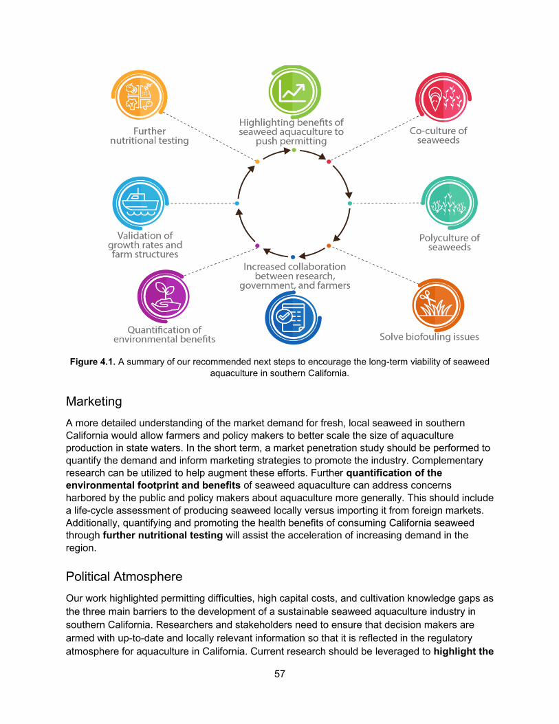
57

Figure 4.1. A summary of our recommended next steps to encourage the long-term viability of seaweed

aquaculture in southern California.

Marketing

A more detailed understanding of the market demand for fresh, local seaweed in southern

California would allow farmers and policy makers to better scale the size of aquaculture

production in state waters. In the short term, a market penetration study should be performed to

quantify the demand and inform marketing strategies to promote the industry. Complementary

research can be utilized to help augment these efforts. Further quantification of the

environmental footprint and benefits of seaweed aquaculture can address concerns

harbored by the public and policy makers about aquaculture more generally. This should include

a life-cycle assessment of producing seaweed locally versus importing it from foreign markets.

Additionally, quantifying and promoting the health benefits of consuming California seaweed

through further nutritional testing will assist the acceleration of increasing demand in the

region.

Political Atmosphere

Our work highlighted permitting difficulties, high capital costs, and cultivation knowledge gaps as

the three main barriers to the development of a sustainable seaweed aquaculture industry in

southern California. Researchers and stakeholders need to ensure that decision makers are

armed with up-to-date and locally relevant information so that it is reflected in the regulatory

atmosphere for aquaculture in California. Current research should be leveraged to highlight the

58

benefits of seaweed aquaculture and encourage the allocation of funds to support future

studies. This will help foster political favor for the growth of environmentally conscious seaweed

production. Increased collaboration between research, government, and farmers can help

overcome the aforementioned barriers that cannot be addressed in isolation. For example,

stakeholders should work together to develop a comprehensive food safety plan for the handling

and sale of locally produced seaweeds. This will give distributors and consumers greater

confidence to buy into domestic production. Additionally, pooling resources encourages the

groundwork to be laid for necessary infrastructure. The establishment of commercial hatcheries

would greatly reduce the initial cost of cultivation for farmers.

Outlook

Taken together, this suite of recommended next steps paves the way for seaweed aquaculture

production in southern California. Stakeholders can use it to create a mutually beneficial

business that is economically sound and ecologically friendly. Current and future Californians

can enjoy a local food item with a rich nutritional profile and few resource inputs. Much like

demand for the product itself, the seaweed industry will most likely not bloom in the span of a

season. However, aquaculturists, scientists, and policy makers have the opportunity to make

decisions in the short term to ensure the maturation of an environmentally responsible industry

that will flourish into the future.

59

References

Abbott, I. A., Isabella, A., & Hollenberg, G. J. (1992). Marine algae of California. Stanford

University Press.

Abreu, M. H., Varela, D. A., Henriquez, L., Villarroel, A., Yarish, C., Sousa-Pinto, I., &

Buschmann, A. H. (2009). Traditional vs. multi-trophic aquaculture of Gracilaria chilensis C.

J.

Abreu, M. H., Pereira, R., Yarish, C., Buschmann, A. H., & Sousa-Pinto, I. (2011). IMTA with

Gracilaria vermiculophylla: productivity and nutrient removal performance of the seaweed in

a land-based pilot scale system. Aquaculture, 312(1-4), 77-87.

Ajjabi, L. C., Abaab, M., & Segni, R. (2017). The red macroalga Gracilaria verrucosa in co-

culture with the Mediterranean mussels Mytilus galloprovincialis: productivity and nutrient

removal performance. Aquaculture International. Retrieved from

https://doi.org/10.1007/s10499-017-0206-2

AltaSea at the Port of Los Angeles. (2018). Research and Business Hub. Retrieved from

https://altasea.org/business-hub/.

Asmus, R.M., & Asmus, H. (1991). Mussel beds: limiting or promoting phytoplankton? J. Exp.

Mar. Biol. Ecol., 148, 215-232.

Azevedo, I.C., Marinhoa, G.S., Silva, D.M., & Sousa-Pintoa, I. (2016). Pilot scale land-based

cultivation of Saccharina latissima Linnaeus at southern European climate conditions:

Growth and nutrient uptake at high temperatures. Aquaculture. 459, 166-172.

Bird, J. McLachlan & E. C. Oliveira: productivity and physiological performance. Aquaculture,

293, 211-220.

Blouin, N. A., Brodie, J. A., Grossman, A. C., Xu, P., & Brawley, S. H. (2011). Porphyra: a

marine crop shaped by stress. Trends in plant science, 16(1), 29-37.

Blouin, N., Xiugeng, F., Peng, J., Yarish, C., & Brawley, S. H. (2007). Seeding nets with neutral

spores of the red alga Porphyra umbilicalis (L.) Kützing for use in integrated multi-trophic

aquaculture (IMTA). Aquaculture, 270(1-4), 77-91.

Blue Economy Incubator. (2016) Port of San Diego website. Retrieved from

https://www.portofsandiego.org/business/blue-economy-incubator.html

Bolton, J.J., Robertson-Andersson, D.V., Shuuluka, D., & Kandjengo, L. (2009). Growing Ulva

(Chlorophyta) in integrated systems as a commercial crop for abalone feed in South Africa:

a SWOT analysis. J. Appl. Phycol., 21, 575-583. https://doi.org/10.1007/s10811-008-9385-6

Boratyn, D. C. (2000). U.S. Patent No. 6,136,329. Washington, DC: U.S. Patent and Trademark

Office.

Brandenburg, W. A. (2016). Sustainable farming at sea. Wageningen University.

Brzezinski, M. A., Reed, D. C., Harrer, S., Rassweiler, A., Melack, J. M., Goodridge, B. M., &

Dugan, J. E. (2013). MULTIPLE SOURCES AND FORMS OF NITROGEN SUSTAIN YEAR-

ROUND KELP GROWTH: on the Inner Continental Shelf of the Santa Barbara Channel.

Oceanography, 26(3), 114-123.

Buck, B. H., Nevejan, N., Wille, M., Chambers, M. D., & Chopin, T. (2017). Offshore and Multi-

Use Aquaculture with Extractive Species: Seaweeds and Bivalves. In Aquaculture

Perspective of Multi-Use Sites in the Open Ocean (pp. 23-69). Springer, Cham.

60

Buchholz, C. M., Krause, G., & Buck, B. H. (2012). Seaweed and man. In Seaweed biology (pp.

471-493). Springer, Berlin, Heidelberg.

Buschmann, A. H., Varela, D. A., Hernandez-Gonzalez, M. C., & Huovinen, P. (2008).

Opportunities and challenges for the development of an integrated seaweed-based

aquaculture activity in Chile: determining the physiological capabilities of Macrocystis and

Gracilaria as biofilters. Journal of Applied Phycology, 20(5), 571-577.

Bush, D. (2018, January 15). Personal interview.

CalCOFI Database. (2017). Cast Hydrographic Data [Data file]. Retrieved from

http://calcofi.org/downloads/database/CalCOFI_Database_194903-

201701_csv_18Oct2017.zip

California Coastal Act of 1976, 20 CA Public Resources Code § 30519.5 (2018).

California Department of Fish and Wildlife. (2007). California Fish and Game Code § 15405.

Retrieved from http://codes.findlaw.com/ca/fish-and-game-code/fgc-sect-15405.html

California Department of Fish and Wildlife. (2018). Commonly Harvested Kelp and Other Marine

Algae.

California Department of Fish and Wildlife. (2014). Informational Digest to the Regulations Governing the Harvest of Kelp and other Marine Algae in California.

California Department of Public Health. (2017). Annual Mussel Quarantine - Frequently Asked

Questions (FAQs). Retrieved from https://www.cdph.ca.gov/Programs/CEH/DRSEM/Pag

es/EMB/Shellfish/Annual-Mussel-Quarantine.aspx.

California Fish and Game Commission. (2018). Initial study and mitigated negative declaration

for Santa Barbara Mariculture Company continued shellfish aquaculture operations on state

water bottom lease offshore Santa Barbara, California. Assessed from

https://nrm.dfg.ca.gov/ FileHandler.ashx?DocumentID=153289&inline

California Ocean Science Trust. (2016). Frequently Asked Questions: Harmful Algal Blooms and

California Fisheries Developed in Response to the 2015-16 Domoic Acid Event. Oakland,

California.

Capo, T. R., Jaramillo, J. C., Boyd, A. E., Lapointe, B. E., & Serafy, J. E. (1999). Sustained high yields of Gracilaria (Rhodophyta) grown in intensive large-scale culture. Journal of Applied Phycology, 11(2), 143.

Carl, C., de Nys, R., & Paul, N.A. (2014). The Seeding and Cultivation of a Tropical Species of Filamentous Ulva for Algal Biomass Production. PLos ONE, 9(6): e98700. https://doi.org/10.1371/journal.pone.0098700

Carmona, R., Kraemer, G.P., & Yarish, C. (2005). Exploring Northeast American and Asian species of Porphyra for use in an integrated finfish-algal aquaculture system. Aquaculture, 252(1), 54-65. https://doi.org/10.1016/j.aquaculture.2005.11.049

Charrier, B., Abreu, M. H., Araujo, R., Bruhn, A., Coates, J. C., De Clerck, O., ... & Wichard, T. (2017). Furthering knowledge of seaweed growth and development to facilitate sustainable aquaculture. New Phytologist, 216(4), 967-975.

Chen, J., Xu, P. (2005). Cultured aquatic species information programme. FAO Fisheries and Aquaculture Department. Rome.

Chopin, T., Hanisak, M. D., Koehn, F. E., Mollion, J., & Moreau, S. (1990). Studies on

carrageenans and effects of seawater phosphorus concentration on carrageenan content

and growth of Agardhiella subulata (C. Agardh) Kraft and Wynne (Rhodophyceae,

Solieriaceae). Journal of Applied Phycology, 2(1), 3-16.

Chung, I. K., Oak, J. H., Lee, J. A., Shin, J. A., Kim, J. G., & Park, K. S. (2013). Installing kelp

61

forests/seaweed beds for mitigation and adaptation against global warming: Korean Project

Overview. ICES Journal of Marine Science, 70(5), 1038-1044.

Cohen, I., & Neori, A. (1991). Ulva lactuca biofilters for marine fishpond effluents. I. Ammonia

uptake kinetics and nitrogen content. Botanica Marina, 34(6), 475-482.

Costa-Pierce, B. A. (2002). The 'Blue Revolution'- Aquaculture must go green. World

Aquaculture, 33(4), 4-5.

Couture, J. (2017, June 30). Personal interview.

Cremades, J. (2012). Seaweed Farming in Spain. Netalgae, Final Conference.

Davison, A.V. & Piedrahita, R.H. (2015). Temperature modeling of a land-based aquaculture

system for the production of Gracilaria pacifica: Possible system modifications to conserve

heat and extend the growing season. Aquacultural Engineering, 66, 1-10.

http://doi.org/10.1016/j. aquaeng.2015.01.003

Dawes, C. P. (1995). Suspended cultivation of Gracilaria in the sea. Journal of applied

phycology, 7(3), 303-313.

Dawson, E. Y., & Foster, M. S. (1982). Seashore plants of California (No. 47). Univ of California

Press.

Ding, L., Ma, Y., Huang, B., & Chen, S. (2013). Effects of seawater salinity and temperature on

growth and pigment contents in Hypnea cervicornis J. Agardh (Gigartinales, Rhodophyta).

BioMed research international, 2013.

Doty, M. S., Caddy, J. F., & Santelices, B. (1987). Case studies of seven commercial seaweed

resources. Rome: FAO.

Dring, M., Edwards, M., & Watson, L. (2013). Development and demonstration of viable

hatchery and ongoing methodologies for seaweed species with identified commercial

potential. Marine Institute.

Duke, C.S., Litaker, W., & Ramus, J. (1989) Effect of temperature on nitrogen-limited growth

rate and chemical composition of Ulva curvata (Ulvales: Chlorophyta). Marine Biology, 100,

143-150.

Druehl LD (1980) 'The Development of an Edible Kelp Culture Technology for British Columbia',

II: second annual report. Province of British Columbia, Ministry of Environment, Marine

Resources Branch, Victoria, B.C.

Edwards, M., Watson, L., O'Mahony, F., Connellan, L., Dring, M., & Werner, A. (2011).

Cultivating Laminaria digitata. Aquaculture explained, 26, 72.

FAO. The state of world fisheries and aquaculture 2004. (2004). Rome: FAO.

Fitridge, I., Dempster, T., Guenther, J., & de Nys, R. (2012). The impact and control of

biofouling in marine aquaculture: a review. Biofouling, 28(7), 649-669.

Flavin, K., Flavin, N. & Flahive, B. (2013). Kelp Farming Manual. A Guide to the Processes,

Techniques and Equipment for Farming Kelp in New England Waters. Ocean Approved

LLC. 123p.

Fletcher, R.L. (1995). Epiphytism and fouling in Gracilaria cultivation: an overview. Journal of

Applied Phycology, 7(3), 325-33.

Fleurence, J. (1999). Seaweed proteins: biochemical, nutritional aspects and potential uses.

Trends in Food Science & Technology, 10(1), 25-28.

Fotedar, R. K., & Phillips, B. F. (2011). Recent advances and new species in aquaculture.

Chichester, U.K.: Wiley-Blackwell.

62

Friedlander, M. (2018, March 2). Personal interview.

Friedman, B. (2017, January 25). Personal interview.

Ganesan, M., Thiruppathi, S., & Jha, B. (2006). Mariculture of Hypnea musciformis (Wulfen)

Lamouroux in South east coast of India. Aquaculture, 256(1-4), 201-211.

Garr, A. L., Acosta-Salmon, H., Davis, M., Capo, T. R., & Riche, M. (2009). Artificial diets for

juvenile queen conch: studies examine algae content. Global aquaculture advocate.

Gentry, R. R., Lester, S. E., Kappel, C. V., White, C., Bell, T. W., Stevens, J., & Gaines, S. D.

(2017). Offshore aquaculture: spatial planning principles for sustainable development.

Ecology and Evolution, 7(2), 733-743.

Graham, M. (2017, October 10). Personal interview.

Grote, B. (2016). Bioremediation of aquaculture wastewater: evaluating the prospects of the red

alga Palmaria palmata (Rhodophyta) for nitrogen uptake. Journal of Applied Phycology,

28(5), 3075-3082.

Guthman, J. (2004). Back to the land: the paradox of organic food standards. Environment and

planning A, 36(3), 511-528.

Halling, C., Aroca, G., Cifuentes, M., Buschmann, A. H., & Troell, M. (2005). Comparison of

spore inoculated and vegetative propagated cultivation methods of Gracilaria chilensis in an

integrated seaweed and fish cage culture. Aquaculture International, 13(5), 409-422.

Herrmann, H. (2018, February 13). Personal interview.

Hernández, I., Fernández-Engo, M.A., Pérez-Lloréns, J.L. & Vergara, J.J. (2005). Integrated

outdoor culture of two estuarine macroalgae as biofilters for dissolved nutrients from Sparus

auratus waste waters. J. Appl. Phycol., 17(6), 557-567.

Hirata, H., Yamasaki, S., Maenosono, H., Nakazono, T., Yamauchi, T., & Matsuda, M. (1994).

Relative budgets of pO2 and pCO2 in cage polycultured red sea bream, Pagrus major and

sterile Ulva sp. Suisanzoshoku, 42(2), 377-381.

Holdt, S.L., & Edwards, M.D. (2014). Cost-effective IMTA: a comparison of the production

efficiencies of mussels and seaweed. Journal of Applied Phycology, 26(2), 933-945.

Holdt, S. L., & Kraan, S. (2011). Bioactive compounds in seaweed: functional food applications

and legislation. Journal of applied phycology, 23(3), 543-597.

Huang, Y. M., & Rorrer, G. L. (2002). Optimal temperature and photoperiod for the cultivation of

Agardhiella subulata microplantlets in a bubble‐ column photobioreactor. Biotechnology and

bioengineering, 79(2), 135-144.

Huguenin, J. E. (1976). An examination of problems and potentials for future large-scale

intensive seaweed culture systems. Aquaculture, 9, 313-342.

Israel, A., Levy, I., & Friedlander, M. (2006). Experimental tank cultivation of Porphyra in Israel.

In Eighteenth International Seaweed Symposium (pp. 9-14). Springer, Dordrecht.

Jansen, H.M. (2012). Bivalve Nutrient Cycling: Nutrient turnover by suspended mussel

communities in oligotrophic fjords (PhD thesis). Retrieved from the Wageningen University

PhD Theses database.

Jensen, A. (1996). Present and future needs for algae and algal products. Hydrobiologia

206/261: 15-23.

Jones, A. (2002). An environmental assessment of food supply chains: a case study on dessert

apples. Environmental management, 30(4), 560-576.

63

Kang, Y. H., Kim, S., Lee, J., Chung, I. K., & Park, S. R. (2014). Nitrogen biofiltration capacities

and photosynthetic activity of Pyropia yezoensis Ueda (Bangiales, Rhodophyta):

groundwork to validate its potential in integrated multi-trophic aquaculture (IMTA). Journal of

Applied Phycology, 26(2), 947-955.

Kasteridis, P., & Yen, S.T. (2012). U.S. demand for organic and conventional vegetables: a

Bayesian censored system approach. The Australian Journal of Agricultural and Resource

Economics, 56, 405–425.

Kim, J. K., Kraemer, G. P., Neefus, C. D., Chung, I. K., & Yarish, C. (2007). Effects of temperature and ammonium on growth, pigment production and nitrogen uptake by four species of Porphyra (Bangiales, Rhodophyta) native to the New England coast. Journal of Applied Phycology, 19(5), 431.

Kim, J. K., Kraemer, G. P., & Yarish, C. (2014). Field scale evaluation of seaweed aquaculture as a nutrient bioextraction strategy in Long Island Sound and the Bronx River Estuary. Aquaculture, 433, 148-156.

Kim, J. K., Yarish, C., Hwang, E. K., Park, M., & Kim, Y. (2017). Seaweed aquaculture:

cultivation technologies, challenges and its ecosystem services. Algae, 32(1), 1-13.

Kim, J. K., Kraemer, G. P., & Yarish, C. (2015). Use of sugar kelp aquaculture in Long Island

Sound and the Bronx River Estuary for nutrient extraction. Marine Ecology Progress Series,

531, 155-166.

Knapp, G. (2008). Economic potential for US offshore aquaculture: an analytical approach.

Offshore aquaculture in the United States: Economic considerations, implications &

opportunities, 15.

Kramer, Chin & Mayo, Inc., 1982. Market analysis and preliminary economic analysis for

products of the red seaweed Porphyra. Report to Department of Natural Resources,

Olympia, Washington, 240 pp.

Lander, T.R., Robinson, S.M.C., MacDonald, B.A., & Martin, J.D. (2012). Enhanced growth rates and condition index of blue mussels (Mytilus edulis) held at integrated multitrophic aquaculture sites in the Bay of Fundy. Journal of Shellfish Research 31, 997-1007.

Lane, C. E., Mayes, C., Druehl, L. D., & Saunders, G. W. (2006). A multi‐ gene molecular investigation of the kelp (Laminariales, Phaeophyceae) supports substantial taxonomic re‐organization. Journal of Phycology, 42(2), 493-512.

Langlois, G., Zubkousky-White, V., Christen, J., & Rankin, S. California Department of Public

Health: Center for Environmental Health. (2014). Marine Biotoxin Monitoring Program

Annual Report.

Lem, P. (2016). Just 1 word for Maine’s future: seaweed. Scientific American.

Lester, S., Gaines, S., Costello, C., Washburn, L. (2014). Maximizing the Values of Offshore

Aquaculture Development in the Context of Multiple Ocean Uses. SeaGrant. R/AQ - 134.

Levine, I. (2018, February 17). Personal interview.

Levine, I. A., & Sahoo, D. (2009). Porphyra: Harvesting Gold from the Sea.[India] Bangalore: IK

International Pvt Ltd.

Lewallen E., Lewallen J. (1996). Sea vegetable gourmet cookbook and wildcrafter’s guide.

Mendocino Sea Vegetable Company, Philo, CA.

Lindahl, O., Hart, R., Hernroth, B., Kollberg, S., Loo, L., Olrog, L., Rehnstam-Holm, A.,

Svensson, J., Svensson, S., & Syversen, U. (2005). Improving Marine Water Quality by

Mussel Farming: A profitable solution for Swedish society. Ambio, 34(2).

Lindell, S. (2018, February 1). Personal interview).

64

Lindell, S., Green-Beach, E., Bailey, D., Beals, M., Kim, J. K., & Yarish, C. (2015). Multi-

cropping seaweed Gracilaria tikvahiae with oysters for nutrient bioextraction and sea

vegetables in Waquoit Bay, MA. In National Shellfisheries Association 107th Annual

Meeting, National Shellfisheries Association; Monterey, CA.

Liu, X., Bogaert, K., Engelen, A. H., Leliaert, F., Roleda, M. Y., & De Clerck, O. (2017).

Seaweed reproductive biology: environmental and genetic controls. Botanica Marina, 60(2),

89-108.

Lovell, R. (2017, November 2). Personal interview.

MacArtain, P., Gill, C. I., Brooks, M., Campbell, R., & Rowland, I. R. (2007). Nutritional value of

edible seaweeds. Nutrition reviews, 65(12), 535-543.

MacDonald, G. M. (2007). Severe and sustained drought in southern California and the West:

Present conditions and insights from the past on causes and impacts. Quaternary

International, 173, 87-100.

MacFarlane, C. I. (1966). A report on some aspects of the seaweed industry in the Maritime

Provinces of Canada. Industrial Development Service, Department of Fisheries of Canada.

McDowell Group (2017) Chapter 1. Alaska’s Mariculture Industry Today. Prepared for Alaska

Department of Fish & Game. p 1-50 (Accessed online: https://www.afdf.org/projects/current-

projects/alaska-mariculture-initiative/)

McHugh, D. J. (2003). A guide to the seaweed industry FAO Fisheries Technical Paper 441.

Food and Agriculture Organization of the United Nations, Rome.

Melvin, D. J., T. F. Mumford, W. J. Byce & V. M. Bryant, 1986. Equipment and techniques for

nori farming in Washington: Vol. I. Conchocelis culture, Department of Natural Resources,

Olympia, Washington, 67 pp.

Mendocino Sea Vegetables. (2011). Printable Order Form & Price List. Retrieved 2018, from

https://www.seaweed.net/Words/printorder.html

Miura, A. (1975). Porphyra cultivation in Japan. Advance of phycology in Japan, 273-304.

Moffitt, C. M., & Cajas-Cano, L. (2014). Blue growth: the 2014 FAO state of world fisheries and

aquaculture. Fisheries, 39(11), 552-553.

Monterey Bay Seaweeds. Seaweed Knowledge. Retrieved from

http://www.montereybayseaweeds.com/about-seaweed/.

Mouritsen, O. G. (2012). The emerging science of gastrophysics and its application to the algal

cuisine. Flavour, 1(1), 6.

Mumford, T. F. (1990). Nori cultivation in North America: growth of the industry. Hydrobiologia,

204(1), 89-98.

Nagler, P.L., Glenn, E.P., Nelson, S.G., & Napolean, S. (2003). Effects of fertilization treatment and stocking density on the growth and production of the economic seaweed Gracilaria parvispora (Rhodophyta) in cage culture at Molokai, Hawaii. Aquaculture, 219 (2003), 379-391.

Naldi, M. & Wheeler, P.A. (2002). N-15 measurements of ammonium and nitrate uptake by Ulva fenestrata (chlorophyta) and Gracilaria pacifica (rhodophyta): comparison of net nutrient disappearance, release of ammonium and nitrate, and N-15 accumulation in algal tissue. Journal of Phycology, 38, 135-44.

Nayar, S., & Bott, K. (2014). Current status of global cultivated seaweed production and markets. World Aquac, 45, 32-37.

NEHLA, (2016). NEHLA Leasing and rate policy. Accessed online: https://nelha.hawaii.gov/wp-content/uploads/2013/05/NELHA-Leasing-Policy_Updated-2016.pdf

65

Neori, A., Cohen, I., & Gordin, H. (1991). Ulva lactuca Biofilters for Marine Fishpond Effluents II. Growth Rate, Yield and C:N Ratio. Botanica Marina, 34, 483-489.

Neori, A., Chopin, T., Troell, M., Buschmann, A. H., Kraemer, G. P., Halling, C., Shpigel, M., &

Yarish, C. (2004). Integrated aquaculture: Rationale, evolution and state of the art

emphasizing seaweed biofiltration in modern mariculture. Aquaculture, 231(1-4), 361–391.

Neori A., Shpigel, M., & Scharfstein, B. (2001). Land-based low-pollution integrated mariculture

of fish, seaweed and herbivores: principles of development, design, operation and

economics.

Aquaculture Europe 2001 Book of Abstracts, Eur. Aquac. Soc. Spec. Publ., vol. 29, pp. 190-191

Newell, R.I.E. (1988). Ecological changes in Chesapeake Bay: are they the result of

overharvesting the American oyster, Crassostrea virginica? Chesapeake Research

Consortium Publication, 129, 536-546.

NOAA Fisheries, Fisheries Statistics Division. (2017). Commercial Fisheries Statistics:

Cumulative Trade Data by U.S. Customs District. [Data file]. Retrieved from

https://www.st.nmfs.noaa.gov/pls/webpls/trade_dstrct.data_in?qtype=IMP&qmnth=12&qyear

=2017& qdistrict=%2C+CA&qproduct=%25&qoutput=TABLE

NOAA National Centers for Environmental Information. (2018). Water Temperature Table of All

Coastal Regions [Data file]. Available from https://www.nodc.noaa.gov/dsdt/cwtg/all.html

Nobre, A. M., et al. (2010). Ecological–economic assessment of aquaculture options: comparison between abalone monoculture and integrated multi-trophic aquaculture of abalone and seaweeds. Aquaculture, 306.1, 116-126.

Norman, K., Sepez, J., Lazrus, H., Milne, N., Package, C., Russell, S., ... & Styles, M. (2007). Community Profiles for West Coast and North Pacific Fisheries: Washington, Oregon, California, and Other US States.

Oliveira, E.C., Alveal, K. & Anderson, R.J. (2000). Mariculture of the agar-producing Gracilarioid

red algae. Reviews in Fisheries Sciences, 8(4), 345-377.

Ortiz, J., Uquiche, E., Robert, P., Romero, N., Quitral, V., & Llantén, C. (2009). Functional and

nutritional value of the Chilean seaweeds Codium fragile, Gracilaria chilensis and

Macrocystis pyrifera. European journal of lipid science and technology, 111(4), 320-327.

Pacheco-Ruíz, I., Bolaños-Arias, G., Zertuche-González, J. A., Gálvez-Télles, A., & Cabello-

Pasini, A. (2005). Propagule release and recruitment in Porphyra perforata (Rhodophyta)

from Baja California, Mexico. Botanica Marina, 48(2), 90-95.

Parker, H. S. (1974). The culture of the red algal genus Eucheuma in the Philippines.

Aquaculture, 3(4), 425-439.

Paul, S., Nicholas, A., Tseng, C. K., & Borowitzka, M. (2013). Seaweed and microalgae.

Aquaculture, Second edition, 268-293.

Pauley, G.B., Van Der Raay, B., & Trout, D. (1988). Pacific Oyster. U.S. Biological Report 82

(11.85).

Pereira, R. & Yarish, C. 2008. Mass production of marine macroalgae. In Jørgensen, S. E. &

Fath, B. D. (Eds.) Encyclopedia of Ecology. Vol. 3. Ecological Engineering Elsevier,

Oxford, pp. 2236-2247.

Peteiro, C., & Freire, Ó. (2013). Biomass yield and morphological features of the seaweed Saccharina latissima cultivated at two different sites in a coastal bay in the Atlantic coast of Spain. Journal of applied phycology, 25(1), 205-213.

66

Peteiro, C., Sánchez, N., & Martínez, B. (2016). Mariculture of the Asian kelp Undaria pinnatifida and the native kelp Saccharina latissima along the Atlantic coast of Southern Europe: an overview. Algal research, 15, 9-23.

Petrell, R. J., Tabrizi, K. M., Harrison, P. J., & Druehl, L. D. (1993). Mathematical model of

Laminaria production near a British Columbian salmon sea cage farm. Journal of Applied

Phycology, 5(1), 1-14.

Radulovich, R., Neori, A., Valderrama, D., Reddy, C. R. K., Cronin, H., & Forster, J. (2015).

Farming of seaweeds. Seaweed sustainability—food and non-food applications, 27-60.)

Reed, D. (2018, January 26). Personal interview. Redmond, S., Green, L., Yarish, C., Kim, J., & Neefus, C. (2014). New England seaweed

culture handbook. Rising Tide Sea Vegetables. (n.d). Online order form. http://www.loveseaweed.com/paypal.html

Roesijadi, G., Copping, A.E., Huesemann, M.H., Forster, J., & Benemann, J.R. (2008). Techno -

Economic Feasibility Analysis of Offshore Seaweed Farming for Bioenergy and Biobased

Products (IR Number: PNWD - 3931). Battelle Pacific Northwest Division.

Romero, R. (2009). Recruitment strategies of Ulva and Porphyra in central California.

Salinas, J. M. (1991). Spray system for re-attachment of Gelidium sesquipedale (Clem.) Born. et

Thur.(Gelidiales: Rhodophyta). In International Workshop on Gelidium (pp. 107-117).

Springer, Dordrecht.

Santelices, B. (1999). A conceptual framework for marine agronomy. In Sixteenth International

Seaweed Symposium(pp. 15-23). Springer, Dordrecht.

Sanderson, J.C., Dring, M.J., Davidson, K., & Kelly, M.S. (2012). Culture, yield and

bioremediation potential of Palmaria palmata (Linnaeus) Weber & Mohr and Saccharina

latissima (Linnaeus) C.E. Lane, C. Mayes, Druehl & G.W. Saunders adjacent to fish farm

cages in northwest Scotland. Aquaculture, 354-355(2), 128-135.

https://doi.org/10.1016/j.aquaculture.2012.03.019

Santelices, B. (1991). Production ecology of Gelidium. In International Workshop on Gelidium

(pp. 31-44). Springer, Dordrecht.

Santelices, B. and Doty, M.S. (1989) A review of Gracilaria farming. Aquaculture, 78(1989), 95-

133.

Sautter, L. R., & Thunell, R. C. (1991). Planktonic foraminiferal response to upwelling and

seasonal hydrographic conditions; sediment trap results from San Pedro Basin, Southern

California Bight. The Journal of Foraminiferal Research, 21(4), 347-363.

Shi, H., Zheng, W., Zhang, X., Zhu, M., & Ding, D. (2013). Ecological-economic assessment of

monoculture and integrated multi-trophic aquaculture in Sanggou Bay of China.

Aquaculture, 410-411, 172-178.

Sim, S., Barry, M., Clift, R., & Cowell, S. J. (2007). The relative importance of transport in

determining an appropriate sustainability strategy for food sourcing. The International

Journal of Life Cycle Assessment, 12(6), 422.

Sindermann, C. J. (1982). Proceedings of the Sixth US-Japan Meeting on Aquaculture, Santa

Barbara, California, August 27-28, 1977.

Soto, D. (ed). (2009). Integrated mariculture: a global review (Report No. 529). FAO Fisheries

and Aquaculture Technical Paper. Rome: FAO.

Stellar Biotechnologies, Inc. (2011). Stellar Biotechnologies Announces Significant Expansion of

Keyhole Limpet Hatchery & Sera Production Capability. Retrieved from https://www.stellar

67

biotechnologies.com/media/press-releases/detail/29/stellar-biotechnologies-announces-

significant-expansion-of

Thomas, T. E., & Harrison, P. J. (1987). Rapid ammonium uptake and nitrogen interactions in five intertidal seaweeds grown under field conditions. Journal of Experimental Marine Biology and Ecology, 107(1), 1-8.

Thompson, S. A., Knoll, H., Blanchette, C. A., & Nielsen, K. J. (2010). Population consequences

of biomass loss due to commercial collection of the wild seaweed Postelsia palmaeformis.

Marine Ecology Progress Series, 413, 17-31.

Titlyanov, E. A., & Titlyanova, T. V. (2010). Seaweed cultivation: methods and problems.

Russian Journal of Marine Biology, 36(4), 227-242.

Troell, M., Ronnback, P., Halling, C., Kautsky, N., & Buschmann, A. (1999). Ecological engineering in aquaculture: use of seaweeds for removing nutrients from intensive mariculture. Journal of Applied Phycology, 11(1), 89-97.

Troell, M., Joyce, A., Chopin, T., Neori, A., Buschmann, A.H., & Fang, J.G., 2009. Ecological

engineering in aquaculture—potential for integrated multi-trophic aquaculture (IMTA) in marine

offshore systems. Aquaculture, 297(1), 1-9.

University of California Berkeley, Jepson Herbaria Specimen Portal, University of California,

Berkeley. (2016). Retrieved 2018, from

https://webapps.cspace.berkeley.edu/ucjeps/publicsearch/publicsearch/

U.S. Department of Labor, Bureau of Labor Statistics. (2017, November). Consumer Price

Index. Washington, DC. (Accessed online:

https://data.bls.gov/timeseries/CUUR0000SA0L1E?output_view=pct_12mths)

Valderrama, D., & Anderson, J. L. (2010). Market interactions between aquaculture and

common-property fisheries: Recent evidence from the Bristol Bay sockeye salmon fishery in

Alaska. Journal of Environmental Economics and Management, 59(2), 115-128.

van den Burg, S., Stuiver, M., Veenstra, F., Bikker, P., Contreras, A.L., Paistra, A., Broeze, J.,

Jansen, H., Jak, R., Gerritsen, A., Harmsen, P., Kals, J., Blanco, A., Brandenburg, W., van

Krimpen, M., van Duijin, A.P., & Mulder, W. (2012). A Triple P review of the feasibility of

sustainable offshore seaweed production in the North Sea(LEI Report 13-077). Wageningen

University & Research Centre.

van den Burg, S. W., van Duijn, A. P., Bartelings, H., van Krimpen, M. M., & Poelman, M.

(2016). The economic feasibility of seaweed production in the North Sea. Aquaculture

Economics & Management, 20(3), 235-252.

Ventura Shellfish Enterprise. (2017). Ventura Shellfish Enterprise website. Retrieved from

http://venturashellfishenterprise.com/

Waaland, J. R. (1977). Common seaweeds of the Pacific coast [USA].

Waaland, R. J. (2004). Integrating intensive aquaculture of the red seaweed Chondracanthus

exasperatus. BULLETIN-FISHERIES RESEARCH AGENCY JAPAN, 91-100.

Wakibia, J. G., Anderson, R. J., & Keats, D. W. (2001). Growth rates and agar properties of

three gracilarioids in suspended open-water cultivation in St. Helena Bay, South Africa.

Journal of applied phycology, 13(3), 195-207.

Wallner, M., Lobo, S., Boccanera, N., & SILVA, E. M. (1992). Biomass, carrageenan yield and

reproductive state of Hypnea musciformis (Rhodophyta: Gigartinales) under natural and

experimental cultivated condition. Aquaculture Research, 23(4), 443-451.

68

Walsh, M., & Watson, L. (2011). A market analysis towards the further development of seaweed

aquaculture in Ireland. Irish Sea Fisheries Board, Dublin.

Washburn, L. (2010). SBC LTER: Reference: Sea-surface water temperature, Santa Barbara

Harbor, Santa Barbara, CA, USA, 1955 to present, ongoing [Data file].

http://dx.doi.org/10.6073/pasta/ba67439ac372ec12610488bc115a4b4e

Watson, L., & Dring, M. (2011). Business Plan for the Establishment of a Seaweed Hatchery

and Grow-out Farm. Irish Sea Fisheries Board.

West, J. A. (2005). Long term macroalgal culture maintenance. Algal Culturing Techniques.

Academic Press, New York, 157-163.

West, John, Hilconida P. Calumpong, and Georg Martin. “Chapter 14: Seaweeds." United

Nations Food and Agriculture. (2016).

Winberg, P. C., Skropeta, D., & Ullrich, A. (2011). Seaweed cultivation pilot trials–towards

culture systems and marketable products.

Wynne, M. J., & Loiseaux, S. (1976). Recent advances in life history studies of the Phaeophyta.

Phycologia, 15(3), 435-452.

Xu, X., Loke, M.K., & Leung, P.S. (2015). Is There a Price Premium for Local Food? The Case

of the Fresh Lettuce Market in Hawaii. Agricultural and Resource Economics Review, 44(1),

110-123.

Yang, Y.F., Fei, X.G., Song, J.M., Hu, H.Y., Wang, G.C., & Chung, I.K., (2006). Growth of

Gracilaria lemaneiformis under different cultivation conditions and its effects on nutrient removal

in Chinese coastal waters. Aquaculture, 254(1), 248-255.

Yarish, C., Remond, S., & Kim, J.K. (2012). Gracilaria culture handbook for New England.

Wrack Lines, (72). https://opencommons.uconn.edu/wracklines/72

Yarish, C., Kim, JK., Lindell, S., and KitsPowerll, H. (2017) "Developing an environmentally and

economically sustainable sugar kelp aquaculture industry in southern New England: from

seed to market " (2017). Department of Marine Sciences. Accessed online at:

http://opencommons.uconn.edu/marines

Zertuche-González, J. A., Sánchez-Barredo, M., Guzmán-Calderón, J. M., & Altamirano-

Gómez, Z. (2014). Eisenia arborea JE Areschoug as abalone diet on an IMTA farm in Baja

California, México. Journal of applied phycology, 26(2), 957-960.

69

Appendices

Appendix A: Biology and life-cycle of seaweed

For any agriculture or aquaculture production, understanding the biology and life-cycle of

seaweed species is necessary to cultivate seaweed. The three major seaweed groups are red

(Rhodophyta), green (Chlorophyta), and brown (Phaeophyta) algae; significant differences in

reproductive and life-history modes exist between these groups. Asexual species, such as

Gracilaria pacifica, are capable of producing multiple individuals from the same parent material

through vegetative fragmentation or asexual spores (Wynne and Loiseaux 1976 in Lui et al.,

2017). Conversely, sexual reproduction requires the release and fusion of gametophytes,

forming a zygote that then undergoes cellular growth via mitosis.

The wide variety of reproductive, physiological, and morphological forms amongst seaweeds

results in highly specialized cultivation strategies that must be determined for each species.

Broadly, there are four major steps in the cultivation of macroalgae, which include 1) hatchery,

2) nursery phase, 3) grow-out phase, 4) harvest phase, but not all species require all phases.

The life-cycles of these species drastically affect the cultivation methods and stages required

during farming. Therefore it is crucial to understand the general differences between these

groups and species.

Red seaweeds reproduction is characterized by a tri-phasic reproductive cycle and an

‘alternation of generations,’ which fluctuate between the adult gametophyte (male or female)

and tetrasporophyte stage (Lobban and Harrison, 1994). In Gracilaria, the adult gametophyte

and tetrasporophyte phases are indistinguishable (i.e. isomorphic), and the thalli of both phases

are used for human consumption (Lobban and Harrison, 1994; Charrier et al., 2017).

Out of all cultivated seaweeds, Pyropia spp. has the most complicated life-history which

necessitates a carefully controlled hatchery stage (Levine and Sahoo, 2009). Considerable work

has gone into identifying and attempting to cultivate Pyropia species that can generate foliose

thalli through asexual means and therefore are capable of seeding asexual spores onto the nets

(e.g. Blouin et al., 2007). This bypasses the concelis phase, reducing the large costs and labor

required for the hatchery phase. However, the majority of cultivated Pyropia species require a

hatchery phase.

Within brown seaweeds, Laminaria setchellii gametophytes continue to develop until

environmental cues (e.g. sufficient quantities of blue light) initiate reproduction, and the female

gametophyte releases a pheromone that attracts motile male sperm. For large-scale cultivation,

the environmental conditions that induce sporing and fertilization are carefully controlled for

during the hatchery phase (see section below).

Ulva lactuca, a green species, can be propagated vegetatively in its unattached form (Titlyanov

and Titlyanova, 2010). However, when grow-out occurs offshore spores are seeded onto the net

or line in a hatchery or wild collection phase (Titlyanov and Titlyanova, 2010).

70

Figure A.1. Life-cycle of Gracilaria spp and representative of red seaweed, and a representative of a

species that can propagate vegetatively (Figure from FAO, 1990).

Figure A.2. Life-cycle of Pyropia spp, which is commonly a sexually reproducing species that requires a

hatchery phase (Figure from Blouin et al 2010).

71

Figure A.3. Life-cycle of Laminaria digitata (Figure from Edwards and Watson, 2011).

72

Appendix B: Hydrographic conditions at our farm location in Santa

Barbara, CA

Table B.1. Historic offshore ocean conditions at our farm site in Santa Barbara, CA. See graphs below for

more information (Data sources: Brzezinski et al., 2013; Reed, 2017; CalCOFI, 2018; NOAA, 2018; Time

and Date, 2018; Washburn, 2018).

DIN (µM) Photoperiod

(hrs)

Surface Irradiance

(mol photons /m2d)

Temp (°C) Current

(cm/s)

Salinity

January 3.9 10.12 38.63 14.27 7.31 33.33

February 3.8 10.98 48.25 13.96 7.68 33.38

March 6.5 11.95 58.20 13.80 7.63 33.5

April 7.3 13.05 65.95 14.02 7.69 33.68

May 4.70 13.97 71.18 15.30 7.77 33.68

June 2.00 14.45 66.95 16.40 8.05 33.58

July 1.1 14.23 68.46 17.57 7.18 33.53

August 1.2 13.43 64.96 14.47 6.93 33.48

September 1.20 12.38 56.39 17.80 7.88 33.45

October 1.10 11.33 50.37 17.17 8.44 33.41

November 1.00 10.37 44.16 16.55 8.79 33.44

December 2.50 9.87 43.49 13.90 7.97 33.36

73

Figure B.1. Ocean temperature (°C) at our offshore farm location in Santa Barbara, CA was estimated

from the monthly average over a 13-year time span (2004 to 2017) at CalCOFI station 81.7.43.5.

Temperatures in May, June, September, and December were estimated using historic averages reported

by NOAA for Santa Barbara or gapfilled using an average of adjacent months. Minimum and maximum

temperatures are shown by the ribbon (Data sources: CalCOFI, 2018; NOAA, 2018).

Figure B.2. Concentration of dissolved inorganic nutrients at our offshore farm location in Santa Barbara,

CA was estimated from depth-averaged concentrations of nitrate, nitrate, and ammonium over the period

2002-2012. Original data collection was at sites Arroyo Burro, Arroyo Quemada, and Mohawk Reef. (Data

source: Brzezinski et al. 2013).

74

Figure B.3. Ocean current speed (cm/s) at the farm site was estimated from average and maximum

moored CTD data at Mohawk Reef (2005-2015). Minimum current speed was assumed to be 0 cm/s for

all months. (Data source: Washburn, 2018).

Figure B.4. Average monthly irradiance (2007-2014) in moles of photons per meter squared per day at

our offshore farm location in Santa Barbara, CA. Minimum and maximum irradiance is shown in the

ribbon. (Data source: Reed, 2017).

75

Data sources:

Brzezinski, M.A., D.C. Reed, S. Harrer, A. Rassweiler, J.M. Melack, B.M. Goodridge, and J.E. Dugan.

(2013). Multiple sources and forms of nitrogen sustain year-round kelp growth on the inner

continental shelf of the Santa Barbara Channel. Oceanography 26(3):114–123, http://dx.doi.org/

10.5670/oceanog.2013.53.

CalCOFI. (2018). Hydrographic Cast Data March 1949 – Summer 2018 [Data file]. Retrieved from

http://calcofi.org/downloads/database/CalCOFI_Database_194903-201708_csv_23Mar2018.zip.

NOAA National Oceanographic Data Center. (2018). Water Temperature Table of the Southern Pacific

Coast. Available from https://www.nodc.noaa.gov/dsdt/cwtg/all_meanT.html.

Reed, D. (2017). SBC LTER: Kelp Removal Experiment: Daily photon irradiance at the surface and

seafloor. Santa Barbara Coastal Long Term Ecological Research Project. doi:10.6073/pasta/e25f4

30bb589b4b16a3d97f6da2afe72

Time and Date. (2018). Yearly Sun Graph for Santa Barbara. Available from

https://www.timeanddate.com/sun/usa/santa-barbara

Washburn, L., Gotschalk, C., & Salazar, D. (2018). Santa Barbara Coastal LTER Moored CTD and ADCP

Data at Mohawk Reef (MKO), ongoing since 2005. Available from http://sbc.lternet.edu/cgi-

bin/showDataset.cgi?docid=knb-lter-sbc.2007.

Washburn, L. (2018). SBCLTER: Ocean: Currents and Biogeochemistry: Moored CTD and ADCP Data at

Mohawk Reef (MKO), ongoing since 2005. Santa Barbara Coastal LTER doi:10.6073/pasta/61ebe5fbec

4663479ddae0eb5961d374.

76

Appendix C: Seaweed data

Table C.1. Low and high growth rates for candidate species both offshore and onshore. In some

instances, the most reliable growth estimate found in the literature was a final annual production instead

of daily relative growth rate. These are indicated as such below and the equivalent relative growth rate

was calculated for use in our bioeconomic model.

Species Offshore Growth Onshore Growth Initial Stocking

Density

Max Stocking

Density

Data Sources

Gracilaria

pacifica

1.4 - 3.98%

RGR per day

5.48 – 6.9%

RGR per day

0.4 kg/m;

3.17 kg/m3

11.9 kg/m3 SARC, Halling

et al 2005;

SARC

Ulva spp. 3.3 – 6.67 kg/m2

annual production

10 – 17.6%

RGR per day

0.375 kg/m3 16.7 kg/m2;

27.8 kg/m3

Titlyanov &

Titlyanova

2010; Duke et

al 1989;

Hernandez et

al 2005

Pyropia

perforata

2.96 - 6.52 kg/m2

annual production

10 – 16%

RGR per day

0.313 kg/m3 NA Parker 1974,

Miura 1975;

Kim et al 2007

Laminaria

spp.

7 – 16 kg/m2

annual production

0.85 – 1.3 %

RGR per day

8 kg/m3 NA Peteiro & Freire

2013, Watson

& Dring 2013;

Azevedo et al

2016

Table C.2. Notable ocean condition factors affecting candidate species growth and reproductive period,

peak natural occurrence in Santa Barbara, harvest frequency, and the proposed cultivation season for

each candidate species in offshore aquaculture systems.

Species Factor(s) affecting

growth

Reproductive

Period

Natural Peak

Occurrence

(Bottom)

Harvest

Frequency

Proposed

Cultivation

Season

Gracilaria

pacifica

Nutrients (DIN),

Light

May/July -

October

March -

October

Every 30 days Feb-July

Ulva lactuca,

lobata, spp.

Temperature, Light June - August August -

October

Once a month May-Oct

Pyropia

perforata

Nutrients, Light,

Temperature,

Reproductive

Summer - Fall March-Sep Every 3

months

Dec-April

Laminaria spp. Nutrients,

Temperature,

Reproductive

Summer - Fall August -

December

Once a year October - March

77

Table C.3. Notable seawater condition factors affecting candidate species growth and reproductive

period, peak natural occurrence in Santa Barbara, harvest frequency, and the proposed cultivation

season for each candidate species in onshore aquaculture systems.

Species Factor(s)

affecting

growth

Reprod.

Period

Natural Peak

Occurrence

(Bottom)

Harvest

Frequency

Proposed

Cultivation

Season

Gracilaria

pacifica

Nutrients

(DIN), Light

May/July -

October

March -

October

Weekly Year round

Ulva lactuca,

lobata, spp.

Temperature June – August August -

October

3.5 weeks Year round

Pyropia

perforata

Nutrients,

Light,

Temperature,

Reproductive

Summer - Fall

(spores settle)

March-Sep 2.5 weeks October to

June

Laminaria spp. Nutrients,

Temperature,

Reproductive

Summer - Fall August (peak)

- December

Every 2

months

October - April

Table C-4. Food market related information for California seaweeds.

Species Geographic Range

Commercial Use Nutritional Value Farm Gate Price

Gracilaria pacifica

Alaska to Southern California

Agar/Food thickener Dried (human) Abalone feed

7-13% protein High fiber

Tank Grown: Carlsbad, $15.4-22/kg; Goleta, $8.8-17.6/kg; Monterey, $88/kg

Ulva spp. Alaska to Mexico

Popular edible: dried, toasted, or eaten fresh

13.6% protein

Tank Grown: Monterey $88/kg

Pyropia perforata

Alaska to Baja (Intertidal and upper subtidal)

Dominant product in sushi, typically as dried sheets

36-47% dried protein

Commercial harvest: $8 per oz, bulk $110-143/kg

Laminaria setchellii

Alaska to Mexico (perennial)

Common in soups, often dried

8-15% protein Commercial harvest: Mendocino $97-105/lb (bulk); Sonoma $171/kg

78

Appendix D: Seaweed yield summary

Table D.1. Model farm yield per unit of production

Species Annual Yield per Unit Farm Unit

Ogo 415 kg 1 longline (137 m)

Sea Lettuce 244 kg 1 net (27 m2)

Nori 475 kg 1 net (27 m2)

Kombu 1450 kg 1 longline (137 m)

Table D.2. Comparison of model calculated output and reported final yields taken from literature.

Species On/off Calculated Yield Reported Final Yield

Ogo Offshore 51,818 kg >320,624 kg

Sea Lettuce Offshore 4.68 kg/m2 3.3 – 6.67 kg/m2

Nori Offshore 119.8 kg/net 80 - 160 kg/net

Kombu Offshore 181,183 kg/25 acres 456,000 kg/25 acres

Ogo Onshore 92 kg/1000-L tank 48 kg/1000-L tank

Sea Lettuce Onshore 165 kg/1000-L tank 48 kg/1000-L tank

Nori Onshore 47 kg/1000-L tank 48 kg/1000-L tank

Kombu Onshore 53 kg/1000-L tank 48 kg/1000-L tank

79

Appendix E. Cost information

Table E.1. Costs for offshore cultivation of Gracilaria pacifica and Laminaria setchellii (Watson & Dring,

2011; D. Marquez, pers comm; B. Friedman, pers comm).

Materials

Single line ($US

2017)

Total Farm Cost (US$

2017)

Fixed Dependent Costs

Longline (Nylon rope: 147m/28mm) $612.26 $76,531.88

Anchor rope (60 m x 2) $349.06 $43,632.75

Chain (5m x 2) $130.90 $16,362.50

Buoy ($32 each, 6m spacing) $704.00 $88,000.00

Trawl floats (x 2) $35.34 $4,417.88

Shackles $52.36 $6,545.00

Tying rope $130.90 $16,362.50

Jeyco Anchors (x 2) $960.00 $120,000.00

Deployment $8,175.00

Total cost (125 lines) $380,027.50

Fixed Independent Costs

Boat (8mx2m Yamaha) $30,000.00

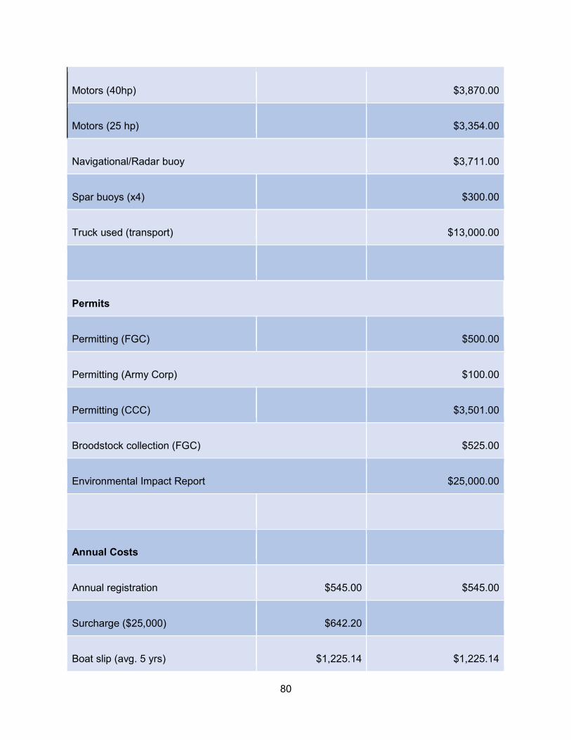
80

Motors (40hp) $3,870.00

Motors (25 hp) $3,354.00

Navigational/Radar buoy $3,711.00

Spar buoys (x4) $300.00

Truck used (transport) $13,000.00

Permits

Permitting (FGC) $500.00

Permitting (Army Corp) $100.00

Permitting (CCC) $3,501.00

Broodstock collection (FGC) $525.00

Environmental Impact Report $25,000.00

Annual Costs

Annual registration $545.00 $545.00

Surcharge ($25,000) $642.20

Boat slip (avg. 5 yrs) $1,225.14 $1,225.14

81

Boat maintenance $2,793.47 $2,793.47

Rent (minimum: $2 if over 10 acres) $250.00 $250.00

Insurance (annual) $2,618.00 $2,618.00

Telephone/postage (annual: harvest

and deployment) $2,356.20 $2,356.20

Diving (annual: harvest and

deployment) $4,188.80 $4,188.80

Protective clothing (annual) $1,309.00 $1,309.00

Annual salary (owner) $50,000.00 $50,000.00

Seeding labor (per) $3,000.00 $3,000.00

Boat maintenance (annual) $2,793.47 $2,793.47

Auto expenses (non-transport) $3,192.40 $3,192.40

Marginal Costs (monthly)

Cost of gas and oil for boat $483.63 $2,898.00

Transport (produce and site) $244.67 $244.67

Auto expenses (non-transport) $266.03 $266.03

Harvest labor (each) $6,000.00 $6,000.00

82

Gracilaria (stocking) $30,825.00 $30,825.00

Table E.2. Costs for offshore cultivation of Pyropia perforata and Ulva lactuca (Levine & Sahoo, 2009;

KMO, 1982; Watson & Dring, 2011).

Material

Pyropia

perforata (US$

2017)

Ulva lactuca

(US$ 2017)

Fixed Dependent Costs

Seeding bags (Hamumbo Sheet) $3,204.36 NA

Nursery frames $55,902.92 NA

Giant wheel for net seeding Missing NA

Nets ($14 each; 18m by 1.5 m) $69,660.00 $19,902.86

Anchors/Anchor line (jeyco anchor) $215,550.00 $215,550.00

Buoy (2 per net) $374,400.00 $374,400.00

Rope-12mm $14,953.68 $14,953.68

Rope-10mm $7,476.84 $7,476.84

Rope-4mm $640.87 $640.87

PVC each net (NA) Missing Missing

Baskets $1,548.00 $1,548.00

83

Net bags $2,018.59 $2,018.59

Equpiment installation $61,920.00 $61,920.00

Fixed Independent Costs

Boat (8mx2m Yamaha) $60,000.00 $30,000.00

Motors (40hp) $7,740.00 $3,870.00

Motors (25 hp) $6,708.00 $3,354.00

Harvester (net) $9,833.93 $4,916.96

Motor (Honda 150-LPO) $4,295.70 $2,147.85

Truck used (transport) $13,000.00 $13,000.00

Navigational/Radar buoy $3,711.02 $3,711.02

Spar buoys (x4) $300.00 $300.00

Cold storage (nets) Missing NA

Permits

Permitting (FGC) $500.00 $500.00

Permitting (Army Corp) $100.00 $100.00

84

Permitting (CCC) $3,501.00 $3,501.00

Broodstock collection (FGC) $525.00 $525.00

Environmental Impact Report $25,000.00 $25,000.00

Annual Costs

Annual registration $545.00 $545.00

Surcharge ($25,000) $642.20 $642.20

Boat slip (avg. 5 yrs) $1,225.14 $1,225.14

Rent (minimum: $2 if over 10 acres) $250.00 $250.00

Boat maintenance $2,793.47 $2,793.47

Insurance (annual) $2,618.00 $2,618.00

Telephone/postage (annual: harvest and deployment) $2,356.20 $2,356.20

Diving (annual: harvest and deployment) $4,188.80 $4,188.80

Protective clothing (annual) $1,309.00 $1,309.00

Annual salary (owner) $50,000.00 $50,000.00

Marginal

Employee (2.5 Fulltime) $57,000.00 NA

85

Employee (deployment) NA $6,000.00

Marginal costs (monthly)

Cost of gas and oil for boat $1,260.00 $483.63

Transport (produce and site) $244.67 $244.67

Auto expenses (non-transport) $266.03 $266.03

Harvest labor (each) NA $6,000.00

Table E.3. Costs for onshore cultivation of seaweed species for a single tank (Watson and Dring, 2011;

D. Marquez, pers comm; D. Bush, pers comm; N. Caruso, pers comm).

Materials

Per unit cost

(US$ 2017)

Tank (1000L) $332.49

Ball valves (2 cm) $23.56

Aerators $7.85

Air Blower: Reischie $1,898.05

Pipework $9.82

Joints, glue, sundries $6.55

Switch gear (installed) $392.70

Shading net (50m2) $3.93

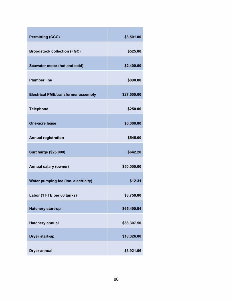
86

Permitting (CCC) $3,501.00

Broodstock collection (FGC) $525.00

Seawater meter (hot and cold) $2,400.00

Plumber line $890.00

Electrical PME/transformer assembly $27,500.00

Telephone $250.00

One-acre lease $6,000.00

Annual registration $545.00

Surcharge ($25,000) $642.20

Annual salary (owner) $50,000.00

Water pumping fee (inc. electricity) $12.31

Labor (1 FTE per 60 tanks) $3,750.00

Hatchery start-up $65,490.94

Hatchery annual $38,307.50

Dryer start-up $18,326.00

Dryer annual $3,921.06

87

Appendix F. Cash flow analyses (cont.)

Figure F.1. The cash flow (thousands of $US) for the payback of Laminaria setchellii and Ulva lactuca at

the break-even price under mean growth scenarios at 5-years in onshore and offshore locations (see

Figure 2.1 for break-even information). The upfront capital costs are labelled on the graph, and include

fixed costs such as permitting and structural costs and costs associated with establishing a hatchery, for

Laminaria setchellii and Ulva lactuca.