UNIVERSITY OF CALIFORNIA, SAN DIEGO

On the Distribution of Oceanic Chlorophyll

A dissertation submitted in partial satisfaction of the

requirements for the degree Doctor of Philosophy

in

Oceanography

by

Benjamin A. Hodges Committee in charge: Professor Daniel L. Rudnick, Chair Professor Peter J. S. Franks Professor Robert Pinkel Professor Sutanu Sarkar Professor William R. Young

2006

Copyright Benjamin A. Hodges, 2006

All rights reserved.

The dissertation of Benjamin A. Hodges is approved, and it is acceptable in quality and form for publication on microfilm:

________________________________________

________________________________________

________________________________________

________________________________________

________________________________________

Chair

University of California, San Diego

2006

iii

DEDICATION

In memory of my grandfather,

Joseph Lawson Hodges Jr.

iv

TABLE OF CONTENTS

Signature Page .……………………………………..………………..…………..iii

Dedication ……………………………………………..………………..………..iv

Table of Contents …………………………………………..………………....….v

List of Figures and Tables …………………………………..…………..……….vii

Acknowledgments ……………………………………………..………..……..…x

Vita, Publications, and Fields of Study ………………………..…………..…….xii

Abstract of the Dissertation ……………………………………..………..……..xiv

Chapter 1 Introduction ………………………………………..……...……….1

Chapter 2 Simple Models of Steady Deep Maxima in Chlorophyll and Biomass ……………………………………………………………5

2.1 Overview …………………………………………………………..6

2.2 Basic Assumptions ………………………………….…………..…8

2.3 How Simple is Too Simple? ……………………………………...10

2.4 Sinking of Phytoplankton …………………………………...……14

2.5 The Effects of Variable Diffusivity ………………………………20

2.6 A Third Compartment …………………………………………….21

2.7 Multiple Phytoplankton Species …………………………………..23

2.8 Discussion …………………………………………………………29

Appendix (Chapter 2) ……………………………………………………..34

Chapter 3 Horizontal Variability in Chlorophyll Fluorescence and Potential Temperature ……………………………………………………….50

3.1 Introduction ………………………………………………………..51

3.2 Spice Cruise ……………………………………………………….54

v

3.3 Scales of Variability ……………………………………………….61

3.4 Temperature-Fluorescence Relationship …………………………..69

3.5 Renovating Wave Model …...……………………………………...71

3.6 Summary and Discussion ………………………………………….79

Appendix (Chapter 3) …………………………………..…………………85

Chapter 4 Glider Observations Along CalCOFI Line 93 ……………...…….110

4.1 Introduction ………………………………………………………110

4.2 Correcting Glider Measurements of Chlorphyll Fluorescence …..112

4.3 Comparison of Glider and CalCOFI Cruise Observations ……….117

4.3.1 Chlorophyll ……………………………………………….117

4.3.2 Salinity ……………………………………………………119

4.4 Response of the Deep Chlorophyll Maximum to Vertical Displacement …………………………………………………..…121

4.5 Summary ………...……………………………………………….123

References ……………………………………………………………………..…139

vi

LIST OF FIGURES AND TABLES

Figure 2.1. Vertical profiles of chlorophyll fluorescence and beam attenuation coefficient from the eastern equatorial Pacific …….….36

Figure 2.2. Vertical profiles of chlorophyll fluorescence and beam attenuation coefficient from near Hawaii …….……………………37

Figure 2.3. Nutrient and phytoplankton profiles from a simple model ………..38 Figure 2.4. Nutrient and phytoplankton profiles from a simple model with

sinking phytoplankton ………………………………….……...…..39 Figure 2.5. Balance of terms in Eq. 2.7 and vertical fluxes from the model ..…40 Figure 2.6. Chlorophyll concentration at the surface and the DCM, and

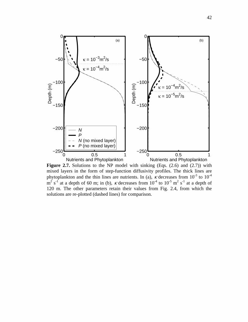
DCM depth as functions of model parameters ……..……………...41 Figure 2.7. Modeled nutrient and phytoplankton profiles with vertically

varying diffusivity ……………...………………………………….42 Figure 2.8. Nutrient, phytoplankton, and detritus profiles from a three-

compartment model ………………………………………………..43 Figure 2.9. Nutrient, phytoplankton, and detritus profiles from a three-

compartment model with sinking of detritus ………………………44 Figure 2.10. Nutrient, phytoplankton, and chlorophyll profiles from a

model with two phytoplankton species …………………………....45 Figure 2.11. Profiles of nutrients, phytoplankton, and new and regenerated

production from a model with two phytoplankton species ………..46 Figure 2.12. Nutrient, phytoplankton, and chlorophyll profiles from a model

with two phytoplankton species, one of which sinks ……………...47 Figure 2.13. Profiles of nutrients, phytoplankton, and new and regenerated

production from a model with two species of phytoplankton, one of which sinks ….……………………………………….....…..48

Table 2.1. Parameter range over which model solutions were obtained …...…49 Figure 3.1. Chlorophyll and density transect showing SeaSoar tow paths

from the Spice experiment ………………………………………...87 Figure 3.2. Temperature, fluorescence, density, and pressure from the

200 dbar tow (Spice) ………………………………………………88 Figure 3.3. Temperature, fluorescence, density, and pressure from the

50 dbar tow ………………………………………………………..89 Figure 3.4. Temperature, fluorescence, density, and pressure from the

25.5 kg/m3 tow …………………………………………………….90 Figure 3.5. Temperature, fluorescence, density, and pressure from the

24.8 kg/m3 tow …………………………………………………….91 Figure 3.6. Power spectra of density and raw and corrected temperature

and fluorescence from the spice tows ……………………………..92 Figure 3.7. Pressure, density, and fluorescence on a short section of the

24.8 kg/m3 tow …………………………………………………….93

vii

Figure 3.8. Temperature and fluorescence fluctuation PDFs from the 200 dbar tow ………………………………………………………94

Figure 3.9. Temperature and fluorescence fluctuation PDFs from the 50 dbar tow ………………………………………………………..95

Figure 3.10. Temperature and fluorescence fluctuation PDFs from the 25.5 kg/m3 tow ……………………………………………….……96

Figure 3.11. Temperature and fluorescence fluctuation PDFs from the 24.8 kg/m3 tow …………………………………………………….97

Figure 3.12. PDFs of temperature-fluorescence wavelet phase difference from the 200 dbar tow ………………………………………….….98

Figure 3.13. PDFs of temperature-fluorescence wavelet phase difference from the 50 dbar tow ……………………………………………....99

Figure 3.14. PDFs of temperature-fluorescence wavelet phase difference from the 25.5 kg/m3 tow ………………………………………….100

Figure 3.15. PDFs of temperature-fluorescence wavelet phase difference from the 24.8 kg/m3 tow ………………………………………….101

Figure 3.16. Schematic of the renovating wave model flow…………….……..102 Figure 3.17. Passive tracer fields stirred by the RW model ……………………103 Figure 3.18. PDFs of wavelet phase difference for two tracers stirred by

the RW model …………………………………………………….104 Figure 3.19. Single realization and final result of a passive tracer field

stirred by the RW model with diffusion ………………………….105 Figure 3.20. PDFs of wavelet phase difference for two tracers stirred by

the RW model with diffusion …………………………………….106 Figure 3.21. Reactive tracers with two different growth rates stirred by

the RW model …………………………………………………….107 Figure 3.22. PDFs of wavelet phase difference between a conservative

tracer and a reactive one with a slow growth rate ………………..108 Figure 3.23. PDFs of wavelet phase difference between a conservative

tracer and a reactive one with a fast growth rate …………………109 Figure 4.1. Map of glider tracks from 3 deployments on Line 93 ……………125 Figure 4.2. Fluorescence data corrected for nonphotochemical quenching

compared with raw data ………………………………………….126 Figure 4.3. Winter CalCOFI Line 93 chlorophyll and density sections,

upper 200 meters, and mean wintertime section …………………127 Figure 4.4. Spring CalCOFI Line 93 chlorophyll and density sections,

and mean springtime section ……………………………………..128 Figure 4.5. Chlorophyll sections from the first glider deployment, showing

isopycnals and vertically averaged current velocity ……………..129 Figure 4.6. Chlorophyll sections from the second glider deployment …...…..130 Figure 4.7. Chlorophyll sections from the third glider deployment ……...…..131 Figure 4.8. Winter CalCOFI Line 93 salinity and density sections,

upper 500 meters, and mean wintertime section …………………132

viii

Figure 4.9. Spring CalCOFI Line 93 salinity and density sections, and mean springtime section ………………………………….…133

Figure 4.10. Salinity sections from the first glider deployment, showing isopycnals and vertically averaged current velocity ………….…134

Figure 4.11. Salinity sections from the second glider deployment …………...135 Figure 4.12. Salinity sections from the third glider deployment ……....……...136 Figure 4.13. Salinity tongue and corresponding changes in chlorophyll

from the second deployment ………………………………….…137 Figure 4.14. Scatter plot showing relationship of density, density anomaly,

and chlorophyll concentration at the deep chlorophyll max over all three deployments ………………………………………138

ix

ACKNOWLEDGEMENTS

I would like to thank Dan Rudnick for being a great advisor. He was always

available, and never failed to drop what he’d been doing to provide advice and

encouragement when I went to see him. He was consistently upbeat, both during

my productive periods, and during the inevitable lapses in my rate of progress. At

the same time he allowed me the space to develop my own ideas and follow my own

path through the process of learning to be a scientist.

The other members of my committee—Peter Franks, Bill Young, Rob

Pinkel, and Sutanu Sarkar—all taught excellent classes which I was lucky enough to

take. Jeff Sherman patiently taught me the ins and outs of the Spray glider, and the

rest of the IDG group provided support in glider preparation and operation. Glenn

Ierley provided advice on numerical calculations. Thanks are due to the California

Cooperative Oceanic Fisheries Investigations program for making the historical data

I have used in Chapter 4 freely available.

Joe Martin was my office mate for 4 years, and remains a good friend. His

unwavering focus and dogged pursuit of his scientific goals was an inspiration. His

willingness, early on, to answer my Matlab questions also came in handy. Other

friends among the SIO student body who made my graduate school experience a

memorable one were Eric Giddens, Dave Drazen, Steve Grimes, and Ana Sirovic.

For the last 28 years (or at least the 25 that I can remember) my family has

been my ultimate source of support and stability. I got my start in science from my

mom, who taught me at home for five of my elementary school years. From my

x

father I acquired an interest in and an affinity for things mechanical, which have

served me well in the lab and at sea.

Chapter 2, in full, is a reproduction of the material as it appears in Deep-Sea

Research I, 2004, Hodges, B.A., Rudnick, D.L., 51, 999-1015. Chapter 3, in full,

has been accepted for publication in Deep-Sea Research I (July 2006). I (the

dissertation author) was the primary investigator and author of both these

publications; I would like to thank Elsevier, the publisher and copyright holder, for

permission to include them in this dissertation.

My dissertation research was supported by the National Science Foundation

under grants OCE00-02598, OCE98-19521, OCE98-19530, and OCE04-52574.

xi

VITA

2000 B.A., Physics, University of California at Berkeley

2000-2006 Graduate Student Researcher, Scripps Institution of Oceanography, University of California, San Diego 2006 Ph.D., Oceanography Scripps Institution of Oceanography, University of California, San Diego

PUBLICATIONS

Hodges, B.A. and D.L. Rudnick, Horizontal variability in chlorophyll fluorescence and potential temperature, Deep-Sea Research I, in press, July 2006. Hodges, B.A. and D.L. Rudnick, Simple models of steady deep maxima in chlorophyll and biomass, Deep-Sea Research I, 51, 999-1015, 2004.

FIELDS OF STUDY

Major Field: Physical Oceanography

Studies in Descriptive Physical Oceanography Professors M.C. Hendershott, D.H. Roemmich, and L.D. Talley Studies in Data Analysis Professors S. Gille, R. Pinkel, and D.L. Rudnick Studies in Fluid Dyamics and Turbulence Professors S. Sarkar and C.D. Winant Studies in Geophysical Fluid Dynamics Professors P. Cessi and W.R. Young

xii

Studies in Linear and Nonlinear Waves Professors R.T. Guza, M.C. Hendershott, and W.K. Melville Studies in Applied Mathematics Professors G.R. Ierley, S.G. Llewellyn Smith, and R. Salmon Studies in Biological Oceanography and Biological-Physical Interactions Professor P.J.S. Franks Studies in Atmospheric Physics Professor R.C. Somerville

xiii

ABSTRACT OF THE DISSERTATION

On the Distribution of Oceanic Chlorophyll

by

Benjamin A. Hodges

Doctor of Philosophy in Oceanography

University of California San Diego, 2006

Professor Daniel L. Rudnick, Chair

The deep chlorophyll maximum (DCM) is a ubiquitous but poorly

understood feature of the ocean ecosystem. Chapter 2 explores possible

explanations for the existence of the DCM with simple, one-dimensional, steady-

state mathematical models. Sinking of plankton or detritus is shown to be critical in

the formation of a deep maximum in phytoplankton biomass. A model with

species-dependent chlorophyll-to-biomass ratios and growth rate characteristics

demonstrates the formation of a DCM which does not represent a maximum in

biomass.

During the Spice cruise of 1997, SeaSoar measurements were made with 4-

m horizontal resolution on two isopycnals and two isobars along a 1000-km transect

in the northeastern Pacific. Chapter 3 is an investigation, based on these data, of the

relationship between the distribution of chlorophyll and that of temperature.

xiv

Fluctuations in the two tracers tend to align with each other, either in phase or out of

phase, at scales above 10 km. Enhancement of gradients by stirring is shown to be a

likely explanation for this behavior, and models suggest that turbulent diffusion or

rapid phytoplankton growth could be responsible for destroying alignment at small

scales.

Chapter 4 presents results from recent glider measurements along CalCOFI

Line 93. Three glider missions were carried out along the 700-km transect, and

chlorophyll and salinity measurements are compared with historical CalCOFI data.

Sharp, density-compensated salinity fronts are found to be common, often with

corresponding features in the chlorophyll field. The deep chlorophyll maximum

tends to track vertical fluctuations in the depth of nearby isopycnals, but on average

the depth of the DCM does not move as far as that of the isopycnals.

xv

Chapter 1 Introduction

This dissertation examines the distribution of chlorophyll in the ocean, both

vertically and horizontally, and from both a modeling and an observational

perspective. Chapter 2 is an attempt to understand the vertical structure of the

oceanic chlorophyll distribution through a series of simple ecological models.

Chapter 3 makes use of hydrographic and chlorophyll data from long horizontal

instrument tows in the northern Pacific to investigate the horizontal distribution of

chlorophyll and its relationship to water temperature, and develops horizontal

stirring models to suggest explanations for the observed behavior. The fourth and

final chapter describes the use of an autonomous underwater glider to elucidate

physical and biological features of the waters off the coast of southern California by

measuring chlorophyll concentration, temperature, and salinity along a 700-km

transect.

Phytoplankton are by far the dominant primary producers of the ocean,

forming the base of the oceanic food web, and providing the energy which fuels the

entire ocean ecosystem. The role they play in uptake of atmospheric carbon

1

2

dioxide, and subsequent export of carbon to the ocean floor, make them an

important influence on global climate change, as the burning of fossil fuels pumps

greenhouse gasses into the atmosphere. Understanding phytoplankton and the

factors effecting their abundance and distribution is thus an important goal.

Phytoplankton contain chlorophyll a, a molecule which allows them to

convert light absorbed from the sun into chemical energy which fuels life functions

like growth and reproduction. Measuring chlorophyll concentration does not

accurately determine the local abundance of phytoplankton—the ratio of the amount

of chlorophyll contained in a cell to the mass of the cell varies greatly—but

chlorophyll nonetheless provides a useful way of studying the phytoplankton

community. Chlorophyll fluoresces: a fraction of the light it absorbs is re-emitted at

a lower frequency. This property makes chlorophyll concentration a very easily,

cheaply, and quickly measured variable related to phytoplankton biomass, allowing

the collection of information about ecosystem structure over a wide range of spatial

and temporal scales.

Aside from the CalCOFI bottle data used in Chapter 4, all the chlorophyll

data used in the observational portions of this work are obtained from in situ

fluorescence measurements. A fluorometer towed behind a ship for a total of over

5000 kilometers provided the chlorophyll data analyzed in Chapter 3. Another

fluorometer, carried a total distance of almost 4000 kilometers by an underwater

glider, produced the chlorophyll data presented in Chapter 4.

Throughout much of the world’s oceans, chlorophyll concentration increases

markedly from the surface downward, reaching a peak, often quite sharp, before

3

decaying toward zero in the deep dark waters below the euphotic zone. The so-

called deep chlorophyll maximum (DCM), despite its ubiquity, is poorly

understood. Some often-cited qualitative explanations for the creation of the DCM

do not produce a subsurface maximum when implemented in simple mathematical

models. Determining mechanisms which could lead to the formation of a DCM, and

eliminating others which cannot is the task undertaken in Chapter 2. Simple, one-

dimensional, steady-state phytoplankton models are used to test a variety of

mechanisms, and to investigate the influence of parameters such as phytoplankton

growth rate and sinking velocity.

Many observers have described the horizontal distribution of plankton as

‘patchy’. The goal of Chapter 3 is to characterize this patchiness, as expressed in

the chlorophyll field, and explain its origin. Regarding chlorophyll as a passive,

reactive tracer, two mechanisms which could lead to small- and meso-scale structure

in its horizontal distribution are: 1) reaction—chlorophyll sources or sinks, e.g.

spatially varying growth/death rates of phytoplankton; and 2) advection—stirring of

large-scale chlorophyll gradients by ocean currents. If the latter is the dominant

mechanism chlorophyll would be expected to display a distribution statistically

similar to that of a passive conservative tracer. By comparing the distributions of

chlorophyll and temperature, it is possible to estimate to what extent the two tracers

are influenced by the same processes.

CalCOFI cruises have been measuring physical and biological properties of

the water off the southern California coast several times per year for decades,

making this region of the ocean one of the most well-sampled anywhere in the

4

world. The large-scale (~100-1000 km) physical and biological structure and

dynamics of the area are thus well known. This knowledge base provides a context

for interpretation of smaller-scale observations in the region; such observations can

illuminate small-scale processes not resolved by CalCOFI cruises, providing a more

complete understanding of the dynamics of the ecosystem as a whole. Chapter 4

takes a step in this direction, comparing high resolution (~3 km in the horizontal,

and ~1 m in the vertical) glider data from CalCOFI Line 93 with coarser-resolution

measurements made in the same location over the preceding quarter-century.

Chapter 2 Simple Models of Steady Deep Maxima in Chlorophyll and Biomass

Abstract of Chapter 2

Possible mechanisms behind the observed deep maxima in chlorophyll and

phytoplankton biomass in the open ocean are investigated with simple, one-

dimensional ecosystem models. Sinking of organic matter is shown to be critical to

the formation of a deep maximum in biomass in these models. However, the form of

the sinking material is not of primary importance to the system: in models with

sinking of detritus, sinking of one phytoplankton species, and sinking of all

phytoplankton, the effect is qualitatively the same. In the two-compartment nutrient-

phytoplankton model, the magnitude of the deep biomass maximum depends more

strongly on sinking rate and diffusivity than on growth and death rates, while the

depth of the maximum is influenced by all four parameters. A model with two

phytoplankton groups that exhibit distinct growth rate characteristics and

chlorophyll contents shows how a deep chlorophyll maximum could form in the

absence of sinking. In this model, when separate compartments are included for

nitrate and ammonia, it is possible to distinguish between new and regenerated

5

6

production, and the phytoplankton group which makes up the deep chlorophyll

maximum is found to carry out almost all of the new production. Variation of eddy

diffusivity with depth is also investigated, and is found not to fundamentally alter

results from models with constant diffusivity.

2.1 Overview

The deep chlorophyll maximum (DCM) is a ubiquitous feature of many

regions of the world’s oceans (Venrick et al., 1973; Cullen, 1982). As fluorescence

is perhaps the most easily measured biological oceanic variable, the DCM is the

most widely known feature of the ocean ecosystem. A permanent characteristic

throughout much of the tropics, deep chlorophyll maxima are also familiar features

in temperate regions, although usually subject there to strong seasonal variability

(Venrick, 1993; Winn et al., 1995).

Deep maxima in phytoplankton biomass are also common. Such a deep

biomass maximum (DBM) is evident in the tropical eastern Pacific at 5.5° N (Fig.

2.1). Shown here are typical profiles of in vivo fluorescence of chlorophyll a, an

approximate measure of chlorophyll concentration (Lorenzen, 1966), and beam

attenuation coefficient, an approximate measure of particulate organic carbon (POC)

(Bishop, 1999). Prominent deep maxima are evident in both. A DCM often occurs

without an accompanying DBM, however (Winn et al., 1995). This is due to

variation in the chlorophyll-to-biomass ratio, which may vary by as much as a factor

of 10 (Cullen and Lewis, 1988). The effect is exemplified in typical profiles of

fluorescence and beam attenuation coefficient from the tropical Pacific near Hawaii

7

(Fig. 2.2). While a strong DCM is present, there is no significant deep maximum

apparent in POC. A DBM is not implied by the existence of a DCM, and when both

are present they often differ in vertical structure (Kitchen and Zaneveld, 1990;

Fennel and Boss, 2003), so it is important to distinguish between the two signatures.

On the other hand, since the chlorophyll-to-biomass ratio generally increases with

depth in the euphotic zone, the presence of a DBM does typically imply a DCM, and

any mechanism which causes the former also causes the latter.

A number of mechanisms have been proposed for the formation of deep

maxima, and indeed it seems likely that a variety of effects are involved. In a recent

paper, Fennel and Boss (2003) investigate the separation of the DCM and DBM, and

possible causes of each. Efforts to model the DCM date back to 1949, when Riley,

Stommel, and Bumpus tackled the problem in their seminal paper. Several fairly

complex models of the planktonic ecosystem exist (e.g. Jamart et al., 1977; Varela

et al., 1992), which are able to accurately match observations. Rather than striving

to reproduce precisely the features of a specific set of observations, the aim of this

paper is to use simple, one-dimensional ecosystem models to examine the feasibility

of a few basic mechanisms which might give rise to deep maxima in chlorophyll

and biomass.

The models presented here are closed, in the sense that there is no exchange

of material across the model domain boundaries. Since there are essentially no live

phytoplankton deeper than a few hundred meters, most models have been limited to

this region. However, nutrient profiles have typically not reached their asymptotic,

deep-ocean values at the bottom of this layer, so these models include an upward

8

diffusive flux of nutrients through the bottom boundary of their domain. The

magnitude of this flux depends on the position of the bottom boundary, and on the

boundary conditions. As our goal is to understand how vertical distributions of

phytoplankton and variables relevant to their ecosystem arise, we extend our models

to a depth great enough to ensure that all model variables attain their asymptotic

values.

The models are kept as simple as possible, allowing isolation of the most

fundamental processes underlying the complex ecological system. We subscribe to

Occam’s razor, which suggests that the simplest explanation of a phenomenon is

intrinsically best. In addition, a sufficiently simple model allows a full search of

parameter space, permitting a more complete understanding of the mathematical

system than would be possible in models of higher complexity.

2.2 Basic Assumptions

It is convenient and sensible to deal in some currency when modeling the

plankton ecosystem. The most common choice, and the one we make here, is

nitrogen (e.g. Steele, 1974) because it is assumed to be the limiting nutrient of

photosynthetic growth. Thus, P(z) represents the concentration of phytoplankton as

a function of depth in terms of the nitrogen it contains. Minimizing the number of

other forms (compartments) in which the currency can exist is essential if one hopes

to form a simple model. So we begin, in our simplest models, without a zooplankton

compartment; rather than being modeled explicitly, the effects of grazing are

included in the net phytoplankton growth rate. Similarly, we begin with the

9

assumption that all phytoplankton exhibit the same environment-dependent rates of

biological activity, and none of our models include more than two such

phytoplankton groups.

There are several other significant simplifications in our models. Each

variable is treated as a continuum, whereas, of course, real plankton are discrete

(see, e.g. Young, 2001). Only one spatial dimension is modeled (the vertical). Thus,

such phenomena as horizontal patchiness in the distribution of phytoplankton (see

Denman et al., 1977 for a discussion) and the horizontal transport of plankton and

nutrients are not considered. Though the ocean is a time-dependent environment, we

consider only the steady-state solutions to the models. As the DCM is a permanent

feature of large regions of the ocean, it seems reasonable to regard the changes it

undergoes as fluctuations about a steady-state distribution. The models’ intrinsic

time scales, determined by the rates of biological activity and by diffusion and

sinking, coupled with the attenuation length of light, are all of the order of tens of

days for the parameter ranges considered. The steady solution applies if it has been

at least this long since a major perturbation in the system. Modeled light intensity

depends only on depth (i.e. there is no self-shading) and no other properties (except,

sometimes, turbulent diffusivity) are explicit functions of depth. The only process

which is directly affected by light is photosynthetic growth, so depth dependence of

chlorophyll-to-nitrogen ratio, remineralization rate, zooplankton grazing rate, etc. is

not included. The reasoning behind this choice is that allowing explicit vertical

variation in more processes would introduce additional degrees of freedom to the

modeling problem, clouding understanding of the mechanisms at work.

10

2.3 How Simple is Too Simple?

One popular explanation of the deep maxima is outlined by Mann and Lazier

(1996) in their recent textbook: “…a certain amount of nitrate is transported upward

through the nutricline by turbulent diffusion. This process leads to more rapid

growth of the phytoplankton population and the formation of a zone of maximum

phytoplankton biomass, the ‘chlorophyll maximum’, just above the nutricline. The

upper boundary of this zone is set by the supply of nutrients from below, and the

lower boundary is set by the availability of light from above”. A simple model

simulating the process described in the above explanation would have two

compartments: phytoplankton P and nutrients N. The net rate at which nitrogen

flows from N to P may be represented by μ(N,P,z), where z, the vertical coordinate,

is zero at the surface and increases upward.1. μ(N,P,z) is the rate of total

phytoplankton growth minus all losses, including those due to death. If we denote

the turbulent diffusivity by κ(z), we obtain the model equations

⎟⎠⎞

⎜⎝⎛

∂∂

∂∂+−=

∂∂

zN

zzPN

tN κμ ),,( , (2.1)

⎟⎠⎞

⎜⎝⎛

∂∂

∂∂+=

∂∂

zP

zzPN

tP κμ ),,( , (2.2)

1 Our convention, throughout this chapter, will be to use italic capital Roman letters for nitrogen

compartments, italic lower- case Roman letters for independent variables, Greek letters for

parameters which may be functions of independent variables or compartments, and normal-text

capital Roman letters for other (constant) parameters.

11

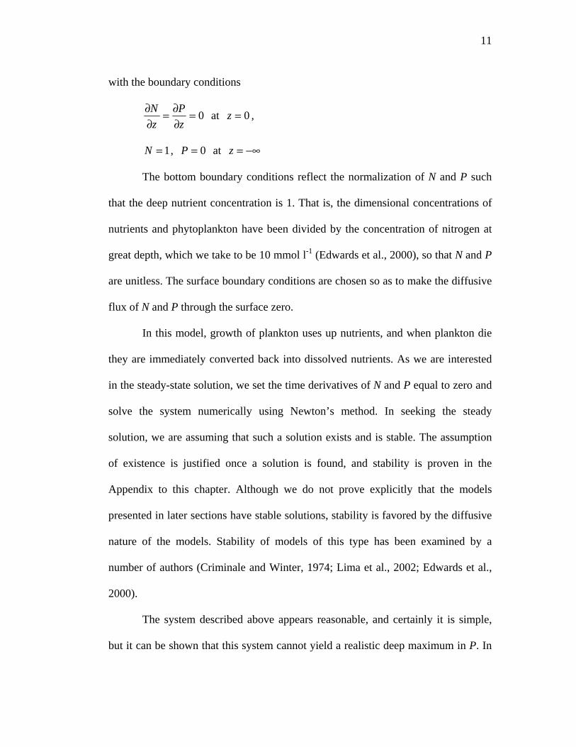
with the boundary conditions

0=∂∂=

∂∂

zP

zN at , 0=z

1=N , at 0=P −∞=z

The bottom boundary conditions reflect the normalization of N and P such

that the deep nutrient concentration is 1. That is, the dimensional concentrations of

nutrients and phytoplankton have been divided by the concentration of nitrogen at

great depth, which we take to be 10 mmol l-1 (Edwards et al., 2000), so that N and P

are unitless. The surface boundary conditions are chosen so as to make the diffusive

flux of N and P through the surface zero.

In this model, growth of plankton uses up nutrients, and when plankton die

they are immediately converted back into dissolved nutrients. As we are interested

in the steady-state solution, we set the time derivatives of N and P equal to zero and

solve the system numerically using Newton’s method. In seeking the steady

solution, we are assuming that such a solution exists and is stable. The assumption

of existence is justified once a solution is found, and stability is proven in the

Appendix to this chapter. Although we do not prove explicitly that the models

presented in later sections have stable solutions, stability is favored by the diffusive

nature of the models. Stability of models of this type has been examined by a

number of authors (Criminale and Winter, 1974; Lima et al., 2002; Edwards et al.,

2000).

The system described above appears reasonable, and certainly it is simple,

but it can be shown that this system cannot yield a realistic deep maximum in P. In

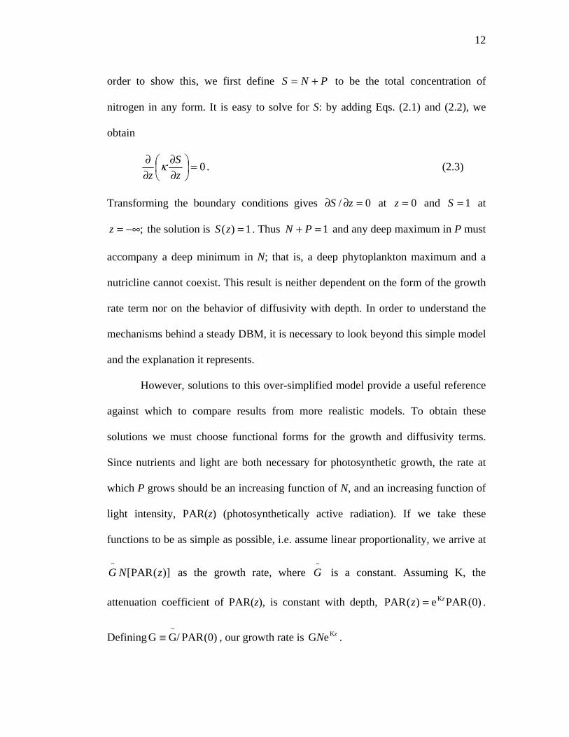
12

order to show this, we first define to be the total concentration of

nitrogen in any form. It is easy to solve for S: by adding Eqs. (2.1) and (2.2), we

obtain

PNS +=

0=⎟⎠⎞

⎜⎝⎛

∂∂

∂∂

zS

zκ . (2.3)

Transforming the boundary conditions gives at and at

the solution is . Thus and any deep maximum in P must

accompany a deep minimum in N; that is, a deep phytoplankton maximum and a

nutricline cannot coexist. This result is neither dependent on the form of the growth

rate term nor on the behavior of diffusivity with depth. In order to understand the

mechanisms behind a steady DBM, it is necessary to look beyond this simple model

and the explanation it represents.

0/ =∂∂ zS 0=z 1=S

;−∞=z 1)( =zS 1=+ PN

However, solutions to this over-simplified model provide a useful reference

against which to compare results from more realistic models. To obtain these

solutions we must choose functional forms for the growth and diffusivity terms.

Since nutrients and light are both necessary for photosynthetic growth, the rate at

which P grows should be an increasing function of N, and an increasing function of

light intensity, PAR(z) (photosynthetically active radiation). If we take these

functions to be as simple as possible, i.e. assume linear proportionality, we arrive at

as the growth rate, where is a constant. Assuming K, the

attenuation coefficient of PAR(z), is constant with depth, .

Defining , our growth rate is

)](PAR[~

zNG~G

)0(PARe)(PAR Kzz =

)0(PAR/GG~

≡ zN KeG .

13

Note that the values assigned to G, sometimes as large as 100 day-1, may

appear at first to be unrealistically high, but that to get a growth rate of G, nutrient

concentration and light level would both have to reach their maximum values (1 in

both the cases) at the same location. As light level is maximum at the surface and

nutrient concentration is maximum at great depth, this never happens, and the actual

phytoplankton growth rate is always much less than G.

Following the Michaelis–Menten equation, a growth rate with a half-

saturation dependence on nutrient or light levels is perhaps more traditional in this

kind of model (Jamart et al., 1977; Franks et al., 1986; Fasham et al., 1990).

However, the euphotic ocean operates mostly at low N, where saturation is

irrelevant, and we have found that such elaborations change the solutions only

slightly. We have therefore opted for simplicity. Adding a constant specific death

rate, D (which includes respiration as well as grazing and other modes of

physiological death), and taking diffusivity to be constant with depth, we obtain the

system

2

2K DeG

zNPNP

tN z

∂∂++−=

∂∂ κ , (2.4)

2

2K DeG

zPPNP

tP z

∂∂+−=

∂∂ κ , (2.5)

with the same boundary conditions as before.

A steady deep phytoplankton maximum is not consistent with this system,

because any such maximum would have to occur in a location darker and poorer in

nutrients, and therefore with a slower growth rate, than the surface. A typical

solution is shown in Fig. 2.3. The parameter values are G = 20 day-1, D = 0.1 day-1,

14

and κ = 10-4 m2s-1. The phytoplankton maximum is, as it must be, at the surface. In

the model equations above, the bottom boundary condition is applied at , but

for computational purposes, we apply this condition at a finite depth deep enough

that change with depth has ceased; in this case the bottom boundary is at 800 m.

Note that in Fig. 2.3 and subsequent figures, only the surface region of this model

domain is depicted, so that near-surface behavior may be more clearly seen.

−∞=z

2.4 Sinking of Phytoplankton

Deep biomass maxima do exist in many areas, particularly in the tropics. In

order to simulate the DBM with our model, the total amount of nitrogen in the

surface layer must be depleted. The simplest mechanism that can maintain a

depletion against the homogenizing effect of diffusion is the sinking of nitrogen.

Accordingly, we introduce a constant phytoplankton sinking rate. The modified

system is

2

2K DeG

zNPNP

tN z

∂∂++−=

∂∂ κ , (2.6)

zP

zPPNP

tP z

∂∂−

∂∂+−=

∂∂ WDeG 2

2K κ , (2.7)

with the boundary conditions

0W =∂∂−=

∂∂

zPP

zN κκ at , 0=z

1=N , at . 0=P −∞=z

15

W is the sinking rate, and the surface boundary condition on P has been changed so

that the total flux of phytoplankton (diffusive plus sinking) through the surface is

zero. The solution has a marked increase in phytoplankton concentration from the

surface to the deep maximum, due to the nitrogen depletion of the surface caused by

sinking of phytoplankton (Fig. 2.4). As long as the chlorophyll-to-biomass ratio is

constant or increasing with depth, this DBM is also a DCM. Of the four terms in the

P equation above (Eq. (2.7)), the dominant balance throughout the euphotic zone is

between growth and death (Fig. 2.5(a)). However, as growth and death only move

nitrogen from one compartment to the other, they do not directly affect the profile of

total nitrogen (N+P). It is a balance between sinking and diffusion that determines

this profile. The flux of total nitrogen must be zero everywhere, so the downward

flux of nitrogen due to the sinking of P is balanced by an upward diffusive flux of

total nitrogen

0W =+∂∂−

∂∂− P

zP

zN κκ . (2.8)

This flux balance is illustrated in Fig. 2.5(b), which shows as functions of depth the

vertical diffusive flux of nutrients (the first term in Eq. (2.8)) and phytoplankton (the

second term), and the vertical flux of phytoplankton due to sinking (the third term).

Sinking of phytoplankton rains nitrogen out of the surface layer, and diffusion

works to replenish it.

The model, in the form above, includes five variable parameters: G, D, κ, K,

and W. We now nondimensionalize the system by scaling the vertical coordinate, z,

by the attenuation length, K-1, and dividing Eqs. (2.6) and (2.7) by D, the death rate.

16

(Note that the variables N and P are already nondimensional, having been scaled by

the limiting nutrient value at depth.) After making the following substitutions:

D/KWG/D,GD,

,K

2*

*

*

*

κ←←

←

←

ttzz

and dropping the asterisks, the nondimensional system obtained looks exactly like

the dimensional system above, except that K and D are equal to unity. The full

parameter space of this model therefore has only three dimensions, and is

investigated rather easily.

Numerical solutions were obtained for the region of parameter space defined

by the (dimensional) values in Table 1. A DBM is a feature in solutions to the

system throughout this entire region. For particularly small sinking velocity and

large diffusivity, the surface concentration of phytoplankton approaches that at the

deep maximum. In these cases, diffusion dominates, and the sinking is not able to

deplete the total nitrogen in the surface layer. In the limit as the ratio κW/K

approaches zero, the model reduces to the trial system of Section 2.3, and the

plankton maximum is at the surface.

Phytoplankton concentration and the depth of the deep maximum vary

considerably across the explored block of G–κ–W parameter space. Each contour

plot in Fig. 2.6 represents a two-dimensional slice through the three-dimensional

parameter space. Because small diffusivities and fast sinking rates deplete the

surface layer of nitrogen, they lead to small phytoplankton concentrations which

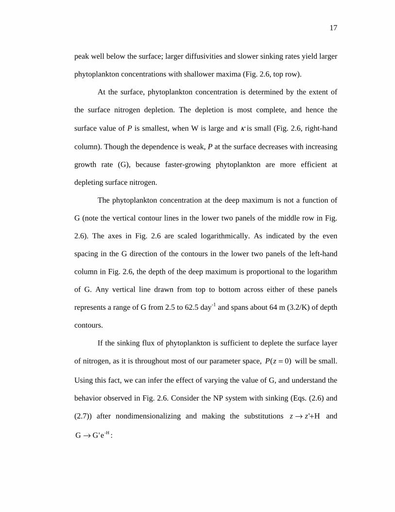
17

peak well below the surface; larger diffusivities and slower sinking rates yield larger

phytoplankton concentrations with shallower maxima (Fig. 2.6, top row).

At the surface, phytoplankton concentration is determined by the extent of

the surface nitrogen depletion. The depletion is most complete, and hence the

surface value of P is smallest, when W is large and κ is small (Fig. 2.6, right-hand

column). Though the dependence is weak, P at the surface decreases with increasing

growth rate (G), because faster-growing phytoplankton are more efficient at

depleting surface nitrogen.

The phytoplankton concentration at the deep maximum is not a function of

G (note the vertical contour lines in the lower two panels of the middle row in Fig.

2.6). The axes in Fig. 2.6 are scaled logarithmically. As indicated by the even

spacing in the G direction of the contours in the lower two panels of the left-hand

column in Fig. 2.6, the depth of the deep maximum is proportional to the logarithm

of G. Any vertical line drawn from top to bottom across either of these panels

represents a range of G from 2.5 to 62.5 day-1 and spans about 64 m (3.2/K) of depth

contours.

If the sinking flux of phytoplankton is sufficient to deplete the surface layer

of nitrogen, as it is throughout most of our parameter space, will be small.

Using this fact, we can infer the effect of varying the value of G, and understand the

behavior observed in Fig. 2.6. Consider the NP system with sinking (Eqs. (2.6) and

(2.7)) after nondimensionalizing and making the substitutions and

:

)0( =zP

H'+→ zz

-He'GG →

18

2

2'

'eG'

zNPNP

tN z

∂∂++−=

∂∂ κ , (2.9)

'W

'eG' 2

2'

zP

zPPNP

tP z

∂∂−

∂∂+−=

∂∂ κ , (2.10)

with the boundary conditions

0'

W'

=∂∂−=

∂∂

zPP

zN κκ at , H' −=z

1=N , at . 0=P −∞='z

This system looks very similar to the original one. The only thing stopping us from

concluding that changing G just amounts to shifting the vertical coordinate is that

the surface boundary condition is applied at , rather than . Now, under

the assumption that P is small near the surface, (9) and (10) may be approximated in

the surface region by

H' −=z 0'=z

.'

W'

,0'

2

2

2

2

zP

zP

zN

∂∂≈

∂∂

≈∂∂

κ

κ

Integrating these from to 0, and applying the BC’s for , we find H' −=z H' −=z

0'

W'

≈∂∂−≈

∂∂

zPP

zN κκ at ,0'=z

which suggests that applying the boundary conditions at provides a

reasonable approximation. Thus if is small, the approximate solution for

where X is an arbitrary constant, may be obtained from the solution for

by shifting it upward by the amount This explains why the

magnitude of the maximum is not a function of G, and why the depth of the

0'=z

)0( =zP

,XGG 0=

0GG = ).Xln(−=Δz

19

maximum changes by about 3.2 attenuation lengths when the value of G changes by

a factor of 25: .2.3)25ln( ≈

Though we have scaled the parameter D out of our model equations by

nondimensionalization, and hence it is not varied in our study of parameter space,

we can still consider the effect of varying the death rate in the original, dimensional

NP model with sinking. Referring back to that system, Eqs. (2.6) and (2.7), we can

see that the solution for the parameter set },D,W,G,{ κ where is the

same as the solution for the parameter set

,XDD 0=

}.D,/W/X,G/X,{ 0Xκ Since we have a

solution set for a single death rate, D0, we can see the result of increasing

(decreasing) the death rate by a given factor by decreasing (increasing) the other

parameters by that same factor. So, for example, since we know that the

phytoplankton concentration at the DBM does not depend on G, we can infer the

dependence of this magnitude on death rate from Fig. 2.6, middle panel, top row.

Changing D corresponds to moving along lines which run across this figure from

lower left to upper right at an angle of 45°. As the contours themselves are nearly

parallel to these lines, the phytoplankton concentration at the maximum is only

weakly affected by the value of the death rate.

In the NP model with sinking, the magnitude of the phytoplankton

concentration is largely a function of the physical variables κ and W and not of the

biological variables G and D (although the sinking rate, W, is certainly influenced

by biology, we classify it as a physical variable because it depends directly on

particle size and density). The biological variables are important, however, in

20

determining the depth of the DBM. As the contours in the lower two panels of the

left-hand column of Fig. 2.6 are more nearly horizontal than vertical, the depth of

the maximum depends more strongly on G than on either of the physical variables.

2.5 The Effects of Variable Diffusivity

The eddy diffusivity, κ, is much larger within the mixed layer than beneath.

It has occasionally been suggested that this transition could be important in the

formation of a deep phytoplankton maximum. In this section, we explore the

consequences of introducing a step-function diffusivity profile into the NP model

with sinking from the previous section. The diffusive terms in the model equations

are rewritten as )/(/ zNz ∂∂∂∂ κ and ),/(/ zPz ∂∂∂∂ κ which are the valid forms when

κ is a function of z.

The effect of introducing a 60-m-deep mixed layer to the model is shown in

Fig. 2.7(a). The value of κ is increased by a factor of 10 in this mixed layer, but

otherwise all parameter values are retained from Fig. 2.4. For comparison, the

nutrient and plankton profiles for the constant-κ case are shown as dashed lines. The

deep maximum is at a depth of approximately 85 m, and so is beneath the base of

the mixed layer. While there are noticeable changes in the profile of phytoplankton

within the mixed layer itself, in the deeper water the profile is essentially unaffected.

Next, consider the less typical case of a mixed layer whose base lies beneath

the deep maximum. Fig. 2.7(b) shows the same ‘reference’ profiles as before

together with the profiles obtained for the case of a 120-m mixed layer. Here, the

21

diffusivity is left unchanged within the mixed layer, but it is decreased by a factor of

10 below the mixed layer base. Maintaining the value of κ at the deep maximum at

10-4 m2 s-1 in both cases allows the resulting profiles to be compared directly with

the reference profile. Once again, the changes induced by the introduction of the

mixed layer are relatively minor. Thus, in our simple models, the characteristics of

the deep maximum depend in large part on the value of κ in the vicinity of the

maximum, and only weakly on the behavior of the profile of κ at other depths.

2.6 A Third Compartment

We have emphasized that sinking is a crucial process in the formation of the

DBM as represented in our simple model with only nutrient and phytoplankton

compartments. The question remains, however, whether a deep phytoplankton

maximum may result from a model without the surface-depleting effect of sinking,

but with additional, nonphytoplankton nitrogen compartments. With this in mind,

we introduce a third compartment, T, here a detrital pool. The new free parameter is

a remineralization rate, R, which governs the transformation of detritus back into

dissolved nutrients, parameterizing nutrient recycling via the microbial loop. The

model equations are

2

2K ReG

zNTNP

tN z

∂∂++−=

∂∂ κ , (2.11)

,DeG 2

2K

zPPNP

tP z

∂∂+−=

∂∂ κ (2.12)

22

,RD 2

2

zTTP

tT

∂∂+−=

∂∂ κ (2.13)

subject to the boundary conditions

0=∂∂=

∂∂=

∂∂

zT

zP

zN at , 0=z

1=N , at . 0== TP −∞=z

Numerical simulations were carried out scanning a large physically and biologically

reasonable region of parameter space similar to the one described for the two-

compartment model in Section 2.4; κ varied from 10-5 to 10-2 m2 s-1, G varied from

1 to 100 day-1, and the remineralization rate, R, took on values from 0.001 to 1.25

day-1. While there is a region of this parameter space in which deep maxima do

occur, the increase in phytoplankton concentration from the surface to the deep

maximum is never as much as 3% of the deep nitrogen concentration. The strongest

such maximum (i.e. the one with the greatest increase in phytoplankton

concentration from the surface to the maximum) occurs when

and is shown in Fig. 2.8. ,s m 0.00082 and ,day 0.0135R ,day 100G 1211 −−− === κ

The third compartment, T, could also be regarded as a zooplankton pool. In

that case, D represents a constant (independent of T) grazing rate, and R a

zooplankton loss rate, including death and excretion. Similar results are found when

the grazing rate is linear in T (when the DP terms in the system above are replaced

by DPT) unless the grazing rate is so large that no stable nontrivial solution exists.

This suggests that, provided they have no explicit depth dependence, no number of

23

additional compartments is likely to lead to the formation of a large and robust

DBM in a simple one-dimensional ecosystem model without sinking.

When sinking of detritus is included in the model above, its behavior is

qualitatively very similar to that displayed by the two-compartment model with

sinking from Section 2.4. Fig. 2.9 shows the solution for this case when the value of

R is 0.2 day-1 and the rest of the parameter values are retained from Fig. 2.4. The

phytoplankton and nutrient profiles are quite similar to those shown in Fig. 2.4; the

biggest difference is that depletion of nitrogen in the surface layer is less effective in

the three-compartment model. The sinking flux is smaller because only detritus

sinks in this case and the concentration of detritus is smaller than is the

concentration of phytoplankton in the NP model. The result is a higher

concentration of phytoplankton at the surface. This slight difference is not due to

any distinct effects of detrital sinking versus sinking of live phytoplankton. Of

primary importance to the model ecosystem is only the magnitude of the sinking

flux of organic matter, not the form that matter takes.

2.7 Multiple Phytoplankton Species

Though sinking is a prerequisite for the formation of a steady DBM in our

NP model, variation with depth in the chlorophyll-to-biomass ratio can lead to a

deep chlorophyll maximum. If photoadaptation is a dominant process in determining

the distribution of chlorophyll—that is, if phytoplankton in deeper water develop

significantly higher chlorophyll-to-biomass ratios in response to the low light

intensity than do those near the surface—a strong DCM may form without a

24

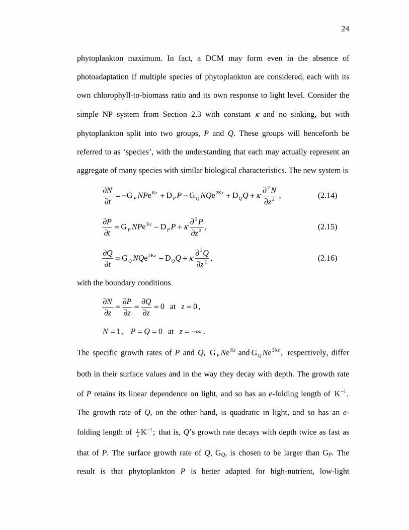
phytoplankton maximum. In fact, a DCM may form even in the absence of

photoadaptation if multiple species of phytoplankton are considered, each with its

own chlorophyll-to-biomass ratio and its own response to light level. Consider the

simple NP system from Section 2.3 with constant κ and no sinking, but with

phytoplankton split into two groups, P and Q. These groups will henceforth be

referred to as ‘species’, with the understanding that each may actually represent an

aggregate of many species with similar biological characteristics. The new system is

2

22KK DeGDeG

zNQNQPNP

tN

Qz

QPz

P ∂∂++−+−=

∂∂ κ , (2.14)

,DeG 2

2K

zPPNP

tP

Pz

P ∂∂+−=

∂∂ κ (2.15)

,DeG 2

2K2

zQQNQ

tQ

Qz

Q ∂∂+−=

∂∂ κ (2.16)

with the boundary conditions

0=∂∂=

∂∂=

∂∂

zQ

zP

zN at , 0=z

1=N , at . 0== QP −∞=z

The specific growth rates of P and Q, respectively, differ

both in their surface values and in the way they decay with depth. The growth rate

of P retains its linear dependence on light, and so has an e-folding length of

The growth rate of Q, on the other hand, is quadratic in light, and so has an e-

folding length of

,eG and eG 2KK zQ

zP NN

.K 1−

;K 121 − that is, Q’s growth rate decays with depth twice as fast as

that of P. The surface growth rate of Q, GQ, is chosen to be larger than GP. The

result is that phytoplankton P is better adapted for high-nutrient, low-light

25

environments, while Q is better adapted for low-nutrient, high-light ones. The

quadratic form of the growth rate of Q is chosen as a simple way to achieve this

adaptive difference between P and Q. One factor which could contribute to

differences in rates of decay of growth rates with depth is that the attenuation

coefficient of light in sea water is frequency dependent, and the absorption spectrum

of phytoplankton varies from species to species (Yentsch and Yentsch, 1979;

Bricaud et al., 1983; Falkowski and Kiefer, 1985). This effect is relatively minor,

however, and here, the dominant factor in the foreshortening of the growth rate

profile is that phytoplankton Q functions less efficiently in lower-light conditions.

The system develops a pronounced deep maximum in P, the species that is

better equipped to survive in dimmer light. The maximum concentration of Q occurs

at the surface. Such vertical separations between different phytoplankton

communities are consistent with observations (e.g. Venrick, 1993). Although the

model still produces no DBM, a DCM may exist if the deeper species has a higher

chlorophyll-to-biomass ratio, a reasonable assumption since a species which lives

mainly in a low-light environment would need more chlorophyll. This effect is

demonstrated in Fig. 2.10, in which plankton P has a chlorophyll-to-biomass ratio

which is larger than that of plankton Q by a reasonable (Bricaud et al., 1983) factor

of four. Biomass has been assumed, here, to be proportional to nitrogen content via

its Redfield ratio to the other major elemental constituents of phytoplankton

(Redfield et al., 1982). Photoadaptation within each species, if included in the

model, would enhance this DCM. Thus the ‘NPQ’ model presented in this section

26

provides a possible explanation of deep chlorophyll maxima which, like that shown

in Fig. 2.2, exist in the absence of a DBM.

It may seem that a DCM formed by the mechanism simulated in this model

would not be of major ecological significance, since it is due to changes in

chlorophyll content and not to phytoplankton abundance. However, this DCM

represents a maximum in a species which dominates at depth, and so monopolizes

the new nutrients diffusing up from below. Thus, the organisms that comprise this

DCM are likely to be responsible for the bulk of the new production (see, e.g.,

Jenkins and Goldman, 1985).

To investigate this aspect of the model system further, we split the nutrient

compartment into new nutrients, N, and recycled or ‘old’ nutrients, O. The N

compartment thus represents nitrate, while O is made up largely of ammonium.

When phytoplankton die, they become O nutrients. The parameter R is a

remineralization rate—the rate at which recycled nutrients are broken down by

bacteria and transformed back into nitrate. In this model, both types of nutrients are

taken up indiscriminately by both types of phytoplankton, so that, for a given set of

parameters, the division of nutrients into two separate compartments has no effect

on the profiles of plankton or of total nutrients. Thus the phytoplankton dynamics of

the model are unchanged, and the division allows a distinction to be made between

new and regenerated production (Fasham et al., 1990). The ‘NOPQ’ system is

,ReGeG 2

2KK

zNONQNP

tN QP z

Qz

P ∂∂++−−=

∂∂ κ (2.17)

,RDeGDeG 2

2KK

zOOQOQPOP

tO

Qz

QPz

PQP

∂∂+−+−+−=

∂∂ κ (2.18)

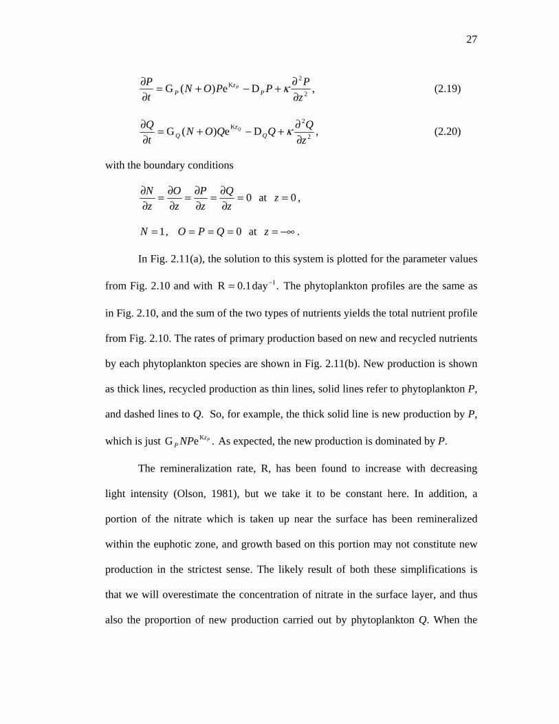
27

,De)(G 2

2K

zPPPON

tP

Pz

PP

∂∂+−+=

∂∂ κ (2.19)

,De)(G 2

2K

zQQQON

tQ

Qz

QQ

∂∂+−+=

∂∂ κ (2.20)

with the boundary conditions

0=∂∂=

∂∂=

∂∂=

∂∂

zQ

zP

zO

zN at , 0=z

1=N , at . 0=== QPO −∞=z

In Fig. 2.11(a), the solution to this system is plotted for the parameter values

from Fig. 2.10 and with The phytoplankton profiles are the same as

in Fig. 2.10, and the sum of the two types of nutrients yields the total nutrient profile

from Fig. 2.10. The rates of primary production based on new and recycled nutrients

by each phytoplankton species are shown in Fig. 2.11(b). New production is shown

as thick lines, recycled production as thin lines, solid lines refer to phytoplankton P,

and dashed lines to Q. So, for example, the thick solid line is new production by P,

which is just As expected, the new production is dominated by P.

.day 1.0R 1−=

.eG K PzP NP

The remineralization rate, R, has been found to increase with decreasing

light intensity (Olson, 1981), but we take it to be constant here. In addition, a

portion of the nitrate which is taken up near the surface has been remineralized

within the euphotic zone, and growth based on this portion may not constitute new

production in the strictest sense. The likely result of both these simplifications is

that we will overestimate the concentration of nitrate in the surface layer, and thus

also the proportion of new production carried out by phytoplankton Q. When the

28

‘false’ new production is eliminated by allowing remineralization only below the

euphotic zone, the main effect is to decrease the rate of new production by

phytoplankton Q even further. Much of the nitrate driving new production in the

euphotic zone is diffused up from beneath, and so must be balanced by export of

nitrogen, in some form, from the euphotic zone. This export is generally attributed

to sinking of organic matter, but in the present model, as there is no sinking, the

export is carried out by diffusion.

Including sinking in the above model allows for a perhaps more realistic

export flux mechanism, and also illustrates the combined effects of surface nitrogen

depletion and variation in chlorophyll-to-biomass ratio. With sinking of

phytoplankton P, the system becomes

,ReGeG 2

2KK

zNONQNP

tN QP z

Qz

P ∂∂++−−=

∂∂ κ (2.21)

,RDeGDeG 2

2KK

zOOQOQPOP

tO

Qz

QPz

PQP

∂∂+−+−+−=

∂∂ κ (2.22)

,WDe)(G 2

2K

zP

zPPPON

tP

PPz

PP

∂∂−

∂∂+−+=

∂∂ κ (2.23)

.De)(G 2

2K

zQQQON

tQ

Qz

QQ

∂∂+−+=

∂∂ κ (2.24)

The boundary conditions are

0W =∂∂=

∂∂−=

∂∂=

∂∂

zQ

zPP

zO

zN

P κ at , 0=z

1=N , at . 0=== QPO −∞=z

29

Only phytoplankton P sinks, but the resulting surface depletion has an

approximately equal impact on both species. Fig. 2.12 shows the solution for P, Q,

and total nutrients (N+O) when the sinking rate, WP, is 1 m day-1, and all other

parameter values are preserved from Fig. 2.10. The maximum concentration of P is

reduced to 48% of its former value when sinking is included, while the maximum

concentration of Q is reduced to 39% of its former value. The chlorophyll maximum

in Fig. 2.12 is the result of two distinct mechanisms; in addition to the stratification

of species with different chlorophyll contents, discussed above, sinking of P gives

rise to a DBM, shown in Fig. 2.12 as the thin solid line, which contributes to the

prominence of the DCM.

Because it enhances exchange between different depths, one would expect

sinking of phytoplankton to increase the f-ratio, that is, the relative amount of new

production. Fig. 2.13 shows the solution to the NOPQ model with sinking of

phytoplankton P, and the rates of new and regenerated production. The parameter

values are the same as those in Figs. 2.11 and 2.12. Comparing Fig. 2.13(b) with

Fig. 2.11(b), one can see that while the introduction of sinking has caused a

reduction in the level of absolute primary production, new production makes up

approximately twice as large a fraction of the total—the f-ratio has doubled.

2.8 Discussion

Our approach to plankton modeling is to regard nitrogen conservation as an

explicit constraint. As primary production in most areas of the oligotrophic ocean is

generally considered to be nitrogen limited, biological activity there can be regarded

30

as a competition among species for available nitrogen. Nitrogen may flow between

compartments, or from one location to another, but it is not created or destroyed.

The depletion of nitrogen from the upper regions of the euphotic zone

caused by sinking of organic matter provides a mechanism for the formation of a

DBM in phytoplankton. In a one-dimensional, steady-state, nitrogen-conserving

model of nonmotile phytoplankton, sinking may provide the only reasonable such

mechanism. Many authors, dating back to Riley et al. (1949) have included sinking

of phytoplankton in their models. However, we suspect that the importance of

sinking in determining the distribution of nitrogen with depth has often been under-

appreciated. Our models with sinking of nitrogen in various forms demonstrate that

the important factor in depleting the euphotic zone of nitrogen (and therefore in

forming a DBM) is just that nitrogen sinks. The form of the sinking material,

whether phytoplankton, detritus, or any other form, is far less important in

determining the vertical structure of the ecosystem. Several authors, notably Steele

and Yentsch (1960), have pointed out that a depth-dependent sinking rate can lead

to vertical structure in the phytoplankton profile. While one would expect an

accumulation of phytoplankton where there is a convergence in sinking rate, we

emphasize that the primary importance of sinking in the formation of a deep

phytoplankton maximum lies not in its changes with depth, but in its nitrogen-

depleting effect on the surface layer.

Models that fail to satisfy the fundamental constraint of nitrogen

conservation can produce misleading results. As an example, the model of Varela et

al. (1992, 1994), patterned after that of Jamart et al. (1977), does not conserve

31

nitrogen. Though their model does not have an explicit zooplankton compartment,

they do include terms representing zooplankton grazing, which removes

phytoplankton from the system, and zooplankton excretion, which adds ammonia.

As grazing is very much larger than excretion, there is a net removal of nitrogen. At

steady state, this loss is balanced by upward diffusion of nitrate from an infinite

reservoir at the bottom of the model domain. It is unlikely that Varela et al. (1994)

would have written that “sinking [was] not needed to reproduce the main DCM

features” had they not achieved surface nitrogen depletion by allowing nitrogen to

vanish from the euphotic zone.

A parameter study of our NP model with sinking provides information about

how parameter values influence the size, shape, and depth of the deep maximum.

Perhaps counterintuitively, the value of the phytoplankton growth rate, G, has no

influence on the magnitude or shape of the deep maximum, but only on its depth.

The depth of the maximum is determined by the growth rate, the sinking rate, and

diffusivity, but the dependence is strongest on growth rate. Thus, the magnitude of

the maximum is a function of diffusivity and sinking rate, while its depth is largely

determined by the growth rate.

Changes in diffusivity with depth, whether these changes occur shallower or

deeper than the DBM, do not have a strong effect on its location or magnitude in our

NP model. Thus the model does not support the hypothesis, suggested, e.g., by

Mann and Lazier (1996), that vertical variation in diffusivity is instrumental in

determining the depth of the DBM.

32

In our models, some factors were found to be of secondary importance in

determining the form of the phytoplankton profile. The basic behavior of this profile

is captured in a two-compartment model subject to removal of surface nitrogen by

sinking. Including additional compartments, such as detritus and zooplankton, does

not profoundly affect phytoplankton concentration. The growth rate terms in the

models presented here are simple functions of nutrient concentration and light

intensity because more complicated forms, when included, were found to introduce

only slight changes to the solutions obtained with the simpler forms.

As chlorophyll-to-biomass ratio may change with depth for a number of

reasons, a DCM may be caused by a wider variety of mechanisms than a DBM. One

such reason is that chlorophyll content varies between species, and species

composition is a function of depth. Even though it is not a DBM, a DCM formed in

this way may be of ecological interest as the dominant region of new production.

That the deep-living species making up the DCM may carry out most of the new

production has been suggested before (Venrick, 1993); our NOPQ model illustrates

one way this pattern could come about. When sinking of phytoplankton is included

in the NOPQ model, a DBM forms, and the f-ratio increases.

The processes highlighted in our models suggest measurements which could

test the validity of the models. If, for example, a DBM arises due to surface nitrogen

depletion caused by sinking of phytoplankton or detritus, then a census of total

nitrogen, including all the particulate forms and dissolved organic and inorganic

nitrogen, should reveal this depletion. The sinking flux of nitrogen in organic

materials, which could possibly be measured with sediment traps, should be

33

sufficient to maintain a surface depletion against the upward eddy diffusion of

nitrate, which could be inferred from the nitrate profile coupled with eddy

diffusivity estimates from dissipation measurements. If a DCM is observed, but

measurements determine that surface nitrogen is not depleted, the sinking

mechanism is ruled out, and the DCM is likely caused by variation in the

chlorophyll-to-nitrogen ratio. In that case, if the ‘NPQ’ process is important in

determining this ratio, the differences between species in chlorophyll content and in

the variation of growth rates with light level should be verifiable.

Acknowledgements. We thank Glenn Ierley, Peter Franks, Bill Young,

Emmanuel Boss, and three reviewers for many helpful comments. We gratefully

acknowledge the support of the National Science Foundation through Grants OCE-

0002598, OCE-9819521, and OCE-9819530. Chapter 2, in full, is a reproduction

of the material as it appears in Deep-Sea Research I, 2004, Hodges, B.A., Rudnick,

D.L., 51 999-1015. The dissertation author was the primary investigator and author

of this paper.

34

Appendix (Chapter 2)

We prove that a stable solution to our first model (Eqs. (2.1) and (2.2))

exists.

⎟⎠⎞

⎜⎝⎛

∂∂

∂∂+−=

∂∂

zN

zzPN

tN κμ ),,( , (1)

⎟⎠⎞

⎜⎝⎛

∂∂

∂∂+=

∂∂

zP

zzPN

tP κμ ),,( , (2)

Boundary conditions:

0=∂∂=

∂∂

zP

zN at , 0=z

1=N , at . 0=P −∞=z

We know that so we can eliminate P from the system: ,1=+ PN

,),(1 ⎟⎠⎞

⎜⎝⎛

∂∂

∂∂+−=

∂∂

⇒−=zN

zzN

tNNP κμ

.),( ⎟⎠⎞

⎜⎝⎛

∂∂

∂∂+

∂∂−=

∂∂

⇒≡∂∂

zN

zNV

tNzN

NV κμ

V is determined by μ up to an arbitrary constant. Note that once this constant is

chosen, since V is bounded for finite μ. Multiplying by and

integrating over z,

],0 ,1[∈N tN ∂∂− /

∫ ∫∞− ∞− ⎥⎦

⎤⎢⎣

⎡∂∂

⎟⎠⎞

⎜⎝⎛

∂∂

∂∂−

∂∂=⎟

⎠⎞

⎜⎝⎛

∂∂−

0 02

.dd ztN

zN

ztVz

tN κ

Integrating the second term on the right-hand side by parts and applying the BC’s,

this becomes

35

∫ ∫∞− ∞− ⎥⎥⎦

⎤

⎢⎢⎣

⎡⎟⎠⎞

⎜⎝⎛

∂∂+=⎟

⎠⎞

⎜⎝⎛

∂∂−

0 022

.d21

ddd z

zNV

tz

tN κ

As long as N is changing with time, the left-hand side is negative, and the integral

on the right-hand side is decreasing. The second term in the integrand is positive,

and V is bounded, so the integral on the right-hand side has a minimum value. N

can only change until this minimum value has been reached, at which point a stable

solution will have been attained.

36

0 0.05 0.1 0.15−250

−200

−150

−100

−50

0

Fluorometer voltage (V)

Dep

th (

m)

0.02 0.04 0.06 0.08 0.1−250

−200

−150

−100

−50

0

Atten. coeff. (m−1)Figure 2.1. Vertical profiles of chlorophyll a fluorescence and beam attenuation coefficient of 660 nm light, a rough measure of POC. The component of attenuation due to absorption by water has been removed. The measurements were made on October 4, 2001, at 5.5° N, 95.4° W, as part of EPIC-2001.

37

0 0.01 0.02 0.03 0.04−250

−200

−150

−100

−50

0

Fluorometer voltage (V)

Dep

th (

m)

0.01 0.02 0.03 0.04 0.05−250

−200

−150

−100

−50

0

Atten. coeff. (m−1)Figure 2.2. Vertical profiles of chlorophyll a fluorescence and beam attenuation coefficient. The data were obtained during the HOME 2002 experiment on October 15, 2002, at latitude 21° N, longitude 159° W.

38

0 0.2 0.4 0.6 0.8 1−250

−200

−150

−100

−50

0

Nutrients and Phytoplankton

Dep

th (

m)

G = 20 day−1

D = 0.1 day−1

κ = 10−4 m2/sPhytoplanktonNutrients

Figure 2.3. Solution to the NP model without sinking, Eqs. (2.4) and (2.5), for the parameter values shown. The profiles of nutrients (dashed) and phytoplankton are mirror images of each other.

39

0 0.2 0.4 0.6 0.8 1−250

−200

−150

−100

−50

0

Nutrients and Phytoplankton

Dep

th (

m)

G = 20 day−1

D = 0.1 day−1

κ = 10−4 m2/sW = −0.5 m/dayPhytoplankton

Nutrients

Figure 2.4. Solution to the NP model with sinking, Eqs. (2.6) and (2.7). Note the pronounced deep maximum in phytoplankton.

40

−0.2 −0.1 0 0.1 0.2−250

−200

−150

−100

−50

0

Upward nitrogen flux (m/day)

Dep

th (

m)

(b)

P (sinking) P (diffusion)N (diffusion)

−0.04 −0.02 0 0.02 0.04−250

−200

−150

−100

−50

0

Terms in P eq. (day−1)

Dep

th (

m)

(a)

Growth Death DiffusionSinking

Figure 2.5. (a) The terms in Eq. (2.7) plotted versus depth for the model solution in Fig. 2.4. The four terms sum to zero, and the dominant balance in the euphotic zone is between growth and death. (b) Vertical flux balance for the same solution. Units on the horizontal axes reflect the fact that nitrogen concentration has been nondimensionalized.

41

0.00005 0.00025 0.001250.1

0.5

2.5

κ (m2/s)

W (

m/d

ay)

Depth of DBM

90

8070

6050

40

0.00005 0.00025 0.001252.5

12.5

62.5

κ (m2/s)

G (

day−

1 )

100

90

8070

60

50

40

30

0.1 0.5 2.52.5

12.5

62.5

W (m/day)

G (

day−

1 )

100

9080

7060

5040

0.00005 0.00025 0.001250.1

0.5

2.5

κ (m2/s)

W (

m/d

ay)

P at DBM

0.1

0.20.3

0.40.5

0.6

0.7

0.8

0.00005 0.00025 0.001252.5

12.5

62.5

κ (m2/s)

G (

day−

1 )

0.1

0.2

0.3

0.4

0.5

0.1 0.5 2.52.5

12.5

62.5

W (m/day)

G (

day−

1 )

0.1

0.2

0.30.

40.5

0.00005 0.00025 0.001250.1

0.5

2.5

κ (m2/s)

W (

m/d

ay)

P at surface

0.1

0.2

0.3

0.4

0.5

0.6

0.7 0.8

0.00005 0.00025 0.001252.5

12.5

62.5

κ (m2/s)

G (

day−

1 )

0.1

0.2

0.3

0.4

0.1 0.5 2.52.5

12.5

62.5

W (m/day)

G (

day−

1 )

0.10.2

0.30.4

Figure 2.6. Behavior of the phytoplankton profile produced by the NP model with sinking (Eqs. (2.6) and (2.7)) as a function of position in G–κ–W parameter space. Depth of the DBM in meters is plotted in the left-hand column, phytoplankton concentration P at the maximum in the middle column, and phytoplankton concentration at the surface in the right-hand column. The dimensional parameter values corresponding to these figures are D = 0.1 day-1 and K = 0.05 m-1. In the upper panels G is constant at 27 day-1; in the middle panels W is constant at -1 m day-1; and in the bottom panels, κ is constant at 10-4 m2 s-1. Note the logarithmic scaling of the axes.

42

0 0.5 1−250

−200

−150

−100

−50

0

Nutrients and Phytoplankton

Dep

th (

m)

0 0.5 1−250

−200

−150

−100

−50

0

Nutrients and Phytoplankton

Dep

th (

m)

N P N (no mixed layer)P (no mixed layer)

κ = 10−3m2/s

κ = 10−4m2/s

κ = 10−4m2/s

κ = 10−5m2/s

(a) (b)

Figure 2.7. Solutions to the NP model with sinking (Eqs. (2.6) and (2.7)) with mixed layers in the form of step-function diffusivity profiles. The thick lines are phytoplankton and the thin lines are nutrients. In (a), κ decreases from 10-3 to 10-4 m2 s-1 at a depth of 60 m; in (b), κ decreases from 10-4 to 10-5 m2 s-1 at a depth of 120 m. The other parameters retain their values from Fig. 2.4, from which the solutions are re-plotted (dashed lines) for comparison.

43

0 0.2 0.4 0.6 0.8 1−250

−200

−150

−100

−50

0

Nutrients, Phytoplankton, and Detritus

Dep

th (

m)

G = 100 day−1

D = 0.1 day−1

R = 0.0135 day−1

κ = 8.2*10−4 m2/s

Nutrients PhytoplanktonDetritus

Figure 2.8. Solution to the NPT model, which includes a detrital compartment but no sinking (Eqs. (2.11), (2.12), and (2.13)). In terms of increase in phytoplankton concentration relative to the surface, this deep maximum is the largest in the region of parameter space described in the text.

44

0 0.2 0.4 0.6 0.8 1−250

−200

−150

−100

−50

0

Nutrients, Phytoplankton, and Detritus

Dep

th (

m)

G = 20 day−1

D = 0.1 day−1

R = 0.2 day−1

W = −0.5 m/dayκ = 4*10−4 m2/s

NutrientsPhytoplanktonDetritus

Figure 2.9. Solution to the three-compartment NPT model with sinking of detritus. The remineralization rate, R, is 0.2 day-1, and the other parameters are the same as in Fig. 2.4, to which this figure may be compared.

45

0 0.2 0.4 0.6 0.8 1−250

−200

−150

−100

−50

0

Nutrients, P, Q, and Chlorophyll

Dep

th (

m)

GP = 15 day−1

GQ

= 60 day−1

DP = 0.1 day−1

DQ

= 0.1 day−1

κ = 5*10−4 m2/s

Nutrients Phytoplankton P Phytoplankton QChlorophyll

Figure 2.10. Solution to the two-phytoplankton NPQ model, Eqs. (2.14), (2.15), and (2.16). The length scale of decay of the growth rate of plankton P is twice that of plankton Q, and P has a chlorophyll-to-biomass ratio four times as large as that of Q. Chlorophyll concentration is plotted with arbitrary units.

46

0 0.5 1−250

−200

−150

−100

−50

0

Nutrients and Phytoplankton

Dep

th (

m)

new N recycled N phytoplankton Pphytoplankton Q

0 0.05 0.1−250

−200

−150

−100

−50

0

Primary production

Dep

th (

m)

new (P) regenerated (P)new (Q) regenerated (Q)

(a) (b)

Figure 2.11. Results from the NOPQ model, Eqs. (2.17)–(2.20). The remineralization rate, R, is 0.1 day-1, and all other parameter values are retained from Fig. 2.10. (a) Solutions to the model equations; thin lines: phytoplankton P (solid) and Q (dashed), thick lines: new (solid) and recycled (dashed) nutrients. (b) Primary production rates; thin lines: regenerated production by P (solid) and Q (dashed), thick lines: new production by P (solid) and Q (dashed). Units of primary production are nitrogen taken up per day as a fraction of the limiting nitrogen concentration at depth.

47

0 0.2 0.4 0.6 0.8 1−250

−200

−150

−100

−50

0

Nutrients, Phytoplankton, and Chlorophyll

Dep

th (

m)

GP = 15 day−1

GQ

= 60 day−1

DP = 0.1 day−1

DQ

= 0.1 day−1

WP = −1 m/day

κ = 5*10−4 m2/s

Phytoplankton P Phytoplankton QTotal biomass Nutrients Chlorophyll

Figure 2.12. Solution to the NPQ model with sinking of phytoplankton P (Eqs. (2.21)–(2.24)). The total phytoplankton biomass, P + Q, is shown as the thin solid line, and total nutrient concentration is the thick dashed line. As in Fig. 2.10, phytoplankton P has four times the chlorophyll content of phytoplankton Q, and chlorophyll is plotted with arbitrary units.

48

0 0.5 1−250

−200

−150

−100

−50

0

Nutrients and Phytoplankton

Dep

th (

m)

new nutrients recycled nutrients phytoplankton P phytoplankton Q

0 0.01 0.02 0.03 0.04−250

−200

−150

−100

−50

0

Primary production

Dep

th (

m)

new (P) regenerated (P)new (Q) regenerated (Q)

(a) (b)

Figure 2.13. As in Fig. 2.11, but with phytoplankton P sinking at 1 m day-1. Note the increase in the ratio of new to regenerated production as compared with Fig. 2.11.

49

Table 2.1. The region of parameter space for which numerical solutions to the NP model with sinking (Eqs. (2.6) and (2.7)) were obtained.

Parameter Symbol Value range Unit

Attenuation coefficient K 0.05 m

Death rate D 0.1 day-1

Growth rate G 2.5 to 62.5 day-1

Diffusivity κ (5 to 125)×10-5 m2s-1

Sinking velocity W -2.5 to -0.1 m day-1

Chapter 3

Horizontal Variability in Chlorophyll Fluorescence and Potential Temperature

Abstract of Chapter 3

Chlorophyll fluorescence and temperature were measured with a horizontal

resolution of 4 meters on two isopycnals and two isobars along a 1000 km

meridional transect in the eastern North Pacific. Probability density functions

(PDFs) of the magnitude of fluctuations in temperature and fluorescence are

compared at each of a large range of length scales. While they are nearly identical

at larger scales, the shapes of the PDFs of fluorescence and temperature differ

significantly at small scales (~1 km and less). This difference may indicate that at

these scales, temperature and fluorescence distributions are controlled by distinct

mechanisms. By comparing the phase of wavelet transforms of each of these two

tracers, the tendency for temperature and fluorescence gradients to line up is

investigated over a large range of spatial scales. At horizontal length scales of order

10 km and larger, the wavelet phase difference between temperature and

fluorescence tends to be close to 0 or 180 degrees--that is, the gradients tend to

align, either in phase or 180 degrees out of phase. At smaller scales, the distribution

50

51

of phase difference on isopycnals is uniform--there is no tendency for gradients to

coincide. Simple stirring models demonstrate that the locations of enhanced

gradients in all tracers would be expected to coincide where the strain has been

greatest. However, the directions of enhanced gradients formed in this way may be

either parallel or antiparallel, depending on initial conditions and on the direction of

the strain. These analyses suggest the horizontal distributions of temperature and

fluorescence at large scales were both governed by advective processes. At

intermediate scales, of order 1-10 km, a renovating wave model suggests that

gradient alignment could be destroyed by turbulent diffusion or by rapid local

phytoplankton growth.

3.1 Introduction

The study of tracers in the ocean has a long history. Any seawater property

that is advected with the flow is a tracer: temperature and salinity characteristics are

useful for distinguishing large-scale water masses (e.g. Iselin, 1939), and on smaller

scales as indicators of local flow patterns (Rudnick and Luyten, 1996). On basin

scales, chlorofluorocarbons are measured to reveal ventilation pathways (e.g.

Smethie and Fine, 2001); on smaller scales, dyes are added to the water to study

dynamics (Ledwell et al., 1993). These tracers may all be described as

conservative—away from formation regions where the tracer properties are set,

there is minimal addition or removal of the tracer. Temperature and salinity are

active, in the sense that they can affect the flow itself through their effect on density.

The other tracers, having no such effect, are referred to as passive.

52

Chlorophyll may also be treated as a passive tracer, but in contrast to the

conservative examples listed above, it is reactive: as phytoplankton grow and die,

chlorophyll is continually created and destroyed. In the ocean interior where mixing

to the surface is not occurring, no heat is transferred into or out of the water, so

potential temperature is a conservative quantity. A comparison of the concurrent

horizontal potential temperature and chlorophyll fields beneath the region of active

surface mixing is then a comparison of conservative and reactive oceanic tracers.

Differences in the statistics of the distributions of these tracers can offer insight into

the different processes determining the structure of their fields (e.g. Martin 2003,

Denman, 1976).

As phytoplankton are the primary producers of the ocean, their spatial

distributions are of fundamental biological importance. Knowledge of these

distributions is also important in the context of climate change, because of the role

of phytoplankton in the global carbon cycle. For these reasons, an understanding of

the mechanisms controlling the distribution of phytoplankton is an important goal.

Plankton ‘patchiness’ has been observed by generations of oceanographers (Hardy,

1936; Cushing, 1961; Denman & Platt, 1976), and is thought to be an important

factor in ecosystem stability (Steele, 1974). However, the causes of this patchiness

are not well understood, and quantitative descriptions of phytoplankton distributions

have often proven elusive, especially at very large and very small scales.

One difficulty lies simply in gathering information that simultaneously spans this

entire range of scales. Such a large dynamic range requires continuous, high-

resolution measurements over long distances. Satellite measurements of ocean color

53

provide information on chlorophyll concentration down to scales of order 1

kilometer, and satellite microwave measurements do the same for sea surface

temperature. However, these measurements only capture variability in the surface

layer of the ocean. To obtain information over a large dynamic range of scales

from deeper layers, it is necessary to tow instruments that measure properties of the

ocean interior in situ.

Perhaps the most easily (and therefore most often) measured biological

property of this sort is chlorophyll fluorescence. When chlorophyll a molecules

absorb visible light, they re-emit some of the energy as light in a wavelength band

near 680 nm. Measurements of the intensity of the fluoresced light are widely used

to estimate chlorophyll concentration, though the relationship between the two

depends somewhat on the particular organisms involved, the extent of quenching,

which depends on their light exposure history, and the degree of ‘packaging’—

essentially self-shading of chlorophyll molecules within an organism (Falkowski

and Kiefer, 1985). As the chlorophyll-to-biomass ratio is highly variable (Pak et al.,

1988; Cullen and Lewis, 1988), chlorophyll concentration alone is not an ideal

indicator of phytoplankton biomass. However, much of the variation in this ratio

may be explained by its dependence on light level and nutrient concentration

(MacIntyre el al., 2002), both of which vary rapidly with depth but weakly with

horizontal distance throughout most of the upper ocean. It is likely, then, that

fluorescence is a better indicator of horizontal than of vertical structure in the

phytoplankton concentration field.

54

When measuring small- to meso-scale horizontal structure of water

properties in the ocean interior, large vertical gradients give rise to a subtler

complication. When an instrument is towed at a constant depth, much of the

variability it records may be due to vertical displacements of the vertical structure

by internal waves. Vertical gradients in temperature and fluorescence are large in

the thermocline and near the deep chlorophyll maximum, respectively, so internal

waves contribute most strongly to the horizontal variability near these locations. In

addition to this ‘horizontal profiling of vertical structure,’ changes occur along

isopycnals, and when interpreting constant-depth measurements, it is difficult to

distinguish between these two sources of horizontal variability. The along-

isopycnal tows described in the following section avoid this difficulty. In addition,

temperature and salinity cancel in their effects on density along isopycnals, and so

lose their distinction as active tracers on these surfaces.

3.2 Spice Cruise

The primary objective of the 1997 Spice experiment (Rudnick and Ferrari,

1999) was to investigate the relationship between seawater temperature and salinity

as a function of depth and horizontal length scale. However, the experiment also

provided an excellent dataset for the study of horizontal variability in chlorophyll

concentration, and of its relationship to physical properties of the water.

The instrumental platform used during the Spice cruise was a SeaSoar,

which is a towed instrument whose depth is controlled by variable-pitch wings.

Instruments on board included a Sea-Bird CTD and a WET Labs WetStar flow-

55

through fluorometer. Fluorometer excitation was centered at a wavelength of 455

nm, and emission measurements were centered at 685 nm. Though the relationship

between fluorometer voltage and chlorophyll concentration is linear ( in

a 14-sample laboratory calibration), we report fluorescence data as volts rather than

converting to chlorophyll concentration because of poorly known species

composition and flow rate in the field, both of which are important for an accurate

calibration. A rough calibration for chlorophyll concentration in mg/m3 in terms of

fluorometer output in volts is . Some of the fluorescence

measurements discussed here were made at depths of 200 meters and deeper. The

proportion of the fluorescence signal comprising live phytoplankton cells is

unknown, but regardless of this proportion, the measurements provide information

on the horizontal structure of the ecosystem.

9987.02 =R

)13.0(16 −= Vchl

The cruise track followed the 140°W meridian back and forth between 25°

and 35°N in the eastern Pacific. The section was repeated five times altogether

between January 24 and February 20, 1997. First, SeaSoar was towed southward

along a sawtooth profile between 5 and 320 dbar, completing one dive

approximately every 3 km. Then, using an automatic dynamic control system, it

followed the 50-dbar isobar northward, and returned southward along the 200-dbar

isobar. The last two tows tracked isopycnals by computing potential density in real

time. The 24.8-kg/m3 isopycnal2 was followed northward until it outcropped near

32°N. The final southward tow tracked the 25.5 kg/m3 isopycnal. The tracks of the

2 Throughout this work, we refer to potential density in terms of its excess over 1000 kg/m3.

56

four horizontal tows are plotted in white in Fig. 3.1, over a section of chlorophyll

fluorescence from the sawtooth tow. The black lines are contours of potential

density, also from the sawtooth tow. The isopycnals moved during the time interval

between the sawtooth and isopycnal tows, so the heavy black lines do not exactly

coincide with the jagged white lines. The horizontal resolution on the horizontal

tows is 4 m, and the RMS deviations from the target surfaces were in the range of

0.4 dbar on the isobars, and 0.02 kg/m3 on the isopycnals.

Along-isopycnal measurements are particularly well-suited to the present

investigation because the short-term influence of internal waves is eliminated.

Transport in the ocean occurs much more readily along isopycnals than across them,

so in the context of mixing, a surface of constant potential density may be regarded

as a single layer, whereas a surface of constant pressure (depth) slices through

multiple layers. Changes observed along isobars are the result of a combination of

isopycnal and diapycnal variability. Interpretation of these isobaric measurements is

therefore less straightforward than that of the isopycnal measurements.

At the southern end of the transect (Fig. 3.1), the deep chlorophyll maximum

lies just beneath the base of the mixed layer, while to the north, it is located within

the mixed layer. Such a transition is a common wintertime feature in this region

(see, e.g., Shulenberger and Reid, 1981). Summertime deep chlorophyll maxima

typically lie well deeper than the mixed layer base. Various processes can

contribute to the formation of the deep chlorophyll maximum, including increase

with depth of mean pigment concentration within cells (Pak et al., 1988), and

57

nitrogen depletion of surface waters by sinking particles (Hodges and Rudnick,

2004).

The location of the deep chlorophyll maximum is important to the

interpretation of the relationship between temperature and fluorescence on an isobar.

Potential temperature typically decreases and potential density increases with depth

throughout the water column, but the vertical gradient of chlorophyll concentration

changes sign at the deep chlorophyll maximum. Thus, on isobars beneath the deep

chlorophyll maximum, vertical movement brings cold, dense, low-chlorophyll water

from below, and warm, light, high-chlorophyll water from above. On these

surfaces, then, vertical displacements will create chlorophyll fluctuations that are in

phase with fluctuations in temperature and out of phase with those in density. The

chlorophyll fluctuations so produced on isobars shallower than the deep chlorophyll

maximum will be out of phase with temperature and in phase with density. On

isobars that cross the deep chlorophyll maximum, both relationships may be seen at

a single depth. Such phase switching has been reported in the past by, for example,

Denman (1976). Changes in growth rate and photoacclimation associated with

vertical motions may act to cancel the alignment of chlorophyll and temperature

fluctuations in some cases and to reinforce it in others.

Fig. 3.2 shows 500-meter averages of data from the 200-dbar isobar tow,

including pressure as well as potential temperature, potential density, and

chlorophyll fluorescence. The strong coherence of the latter three variables over

most of the tow is easily explained—the dominant source of variance in each is

local vertical displacement.

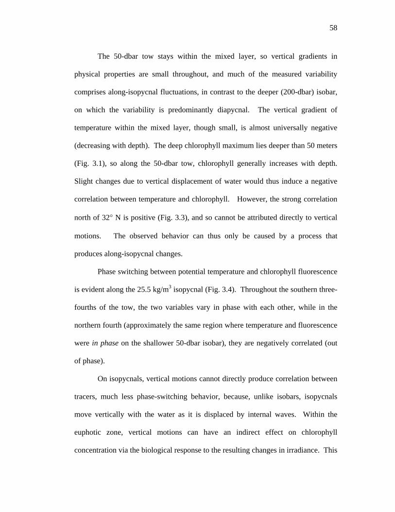
58

The 50-dbar tow stays within the mixed layer, so vertical gradients in

physical properties are small throughout, and much of the measured variability

comprises along-isopycnal fluctuations, in contrast to the deeper (200-dbar) isobar,

on which the variability is predominantly diapycnal. The vertical gradient of

temperature within the mixed layer, though small, is almost universally negative

(decreasing with depth). The deep chlorophyll maximum lies deeper than 50 meters

(Fig. 3.1), so along the 50-dbar tow, chlorophyll generally increases with depth.

Slight changes due to vertical displacement of water would thus induce a negative

correlation between temperature and chlorophyll. However, the strong correlation

north of 32° N is positive (Fig. 3.3), and so cannot be attributed directly to vertical

motions. The observed behavior can thus only be caused by a process that

produces along-isopycnal changes.

Phase switching between potential temperature and chlorophyll fluorescence

is evident along the 25.5 kg/m3 isopycnal (Fig. 3.4). Throughout the southern three-

fourths of the tow, the two variables vary in phase with each other, while in the

northern fourth (approximately the same region where temperature and fluorescence

were in phase on the shallower 50-dbar isobar), they are negatively correlated (out

of phase).

On isopycnals, vertical motions cannot directly produce correlation between

tracers, much less phase-switching behavior, because, unlike isobars, isopycnals

move vertically with the water as it is displaced by internal waves. Within the

euphotic zone, vertical motions can have an indirect effect on chlorophyll

concentration via the biological response to the resulting changes in irradiance. This

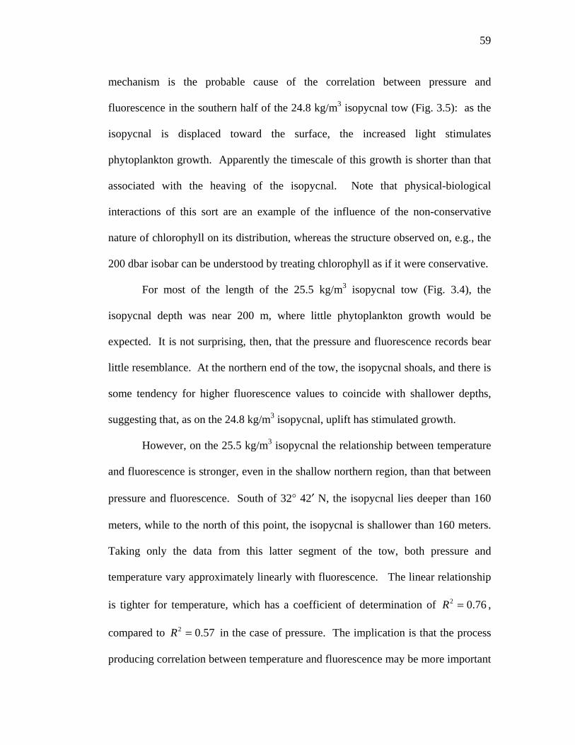
59

mechanism is the probable cause of the correlation between pressure and

fluorescence in the southern half of the 24.8 kg/m3 isopycnal tow (Fig. 3.5): as the

isopycnal is displaced toward the surface, the increased light stimulates

phytoplankton growth. Apparently the timescale of this growth is shorter than that

associated with the heaving of the isopycnal. Note that physical-biological

interactions of this sort are an example of the influence of the non-conservative

nature of chlorophyll on its distribution, whereas the structure observed on, e.g., the

200 dbar isobar can be understood by treating chlorophyll as if it were conservative.

For most of the length of the 25.5 kg/m3 isopycnal tow (Fig. 3.4), the

isopycnal depth was near 200 m, where little phytoplankton growth would be

expected. It is not surprising, then, that the pressure and fluorescence records bear

little resemblance. At the northern end of the tow, the isopycnal shoals, and there is

some tendency for higher fluorescence values to coincide with shallower depths,

suggesting that, as on the 24.8 kg/m3 isopycnal, uplift has stimulated growth.

However, on the 25.5 kg/m3 isopycnal the relationship between temperature

and fluorescence is stronger, even in the shallow northern region, than that between

pressure and fluorescence. South of 32° 42′ N, the isopycnal lies deeper than 160

meters, while to the north of this point, the isopycnal is shallower than 160 meters.

Taking only the data from this latter segment of the tow, both pressure and

temperature vary approximately linearly with fluorescence. The linear relationship

is tighter for temperature, which has a coefficient of determination of ,

compared to in the case of pressure. The implication is that the process

producing correlation between temperature and fluorescence may be more important

76.02 =R

57.02 =R

60

on this isopycnal than the biological response to isopycnal uplift, even in the

shallow segment of the tow. The immunity of along-isopycnal measurements to

‘contamination’ by vertical structure necessitates an alternate explanation for the

observed correlation between temperature and fluorescence on the isopycnal.

Stirring of large-scale gradients provides a likely explanation for both the

behavior observed on the isopycnal and the occurrence of temperature-fluorescence

correlation of the ‘wrong’ sign on the isobars. As a tracer is advected by flow,

filaments form. A blob of tracer is drawn out in a long tendril, stretching along one

dimension as it contracts along another. Any initial gradient in tracer concentration

in the direction of this contraction is amplified as the fluid particles move closer

together. When two initially distant fluid particles in a smooth tracer field approach

each other, a strong concentration gradient typically develops along the line

connecting them. The sign of this gradient (that is, increasing or decreasing)

depends on the initial field. Where the signs of the gradients of two tracers in the

direction of contraction are the same, in-phase behavior develops. Where the signs

of the gradients are opposite, the result is out-of-phase behavior. Thus two initially

unrelated tracers, when advected by a flow, would be expected over time to develop

enhanced gradients in the same locations and along the same directions, but not

necessarily of the same signs. This stirring-induced gradient alignment provides an

attractive explanation of the correlation, positive in some locations and negative in

others, between potential temperature and fluorescence on the 25.5 kg/m3 isopycnal

(Fig. 3.4). It is likely also the mechanism behind the in-phase relationship observed

at 50 dbar (Fig. 3.3).

61

The strong front north of 29° N is clearly visible in both temperature and

fluorescence from the 24.8 kg/m3 isopycnal tow (Fig. 3.5). This feature, like the

structure on the deeper isopycnal, is probably the result of a high degree of strain,

though interpretation is complicated because in the region of the front the isopycnal

is crossing the mixed layer base.

We examine the distribution of potential temperature and chlorophyll

fluorescence on the four horizontal tows in Section 3.3. The range of length scales

on which gradient alignment between these two tracers was observed is the subject

of Section 3.4. In Section 3.5 we use simple stirring models to demonstrate gradient

alignment and investigate the scales on which it occurs.

3.3 Scales of Variability

A basic property of any scalar function of position is the way in which the

variance is distributed among spatial scales. This information is presented (Fig. 3.6)

in spectra of the measurements of potential temperature (blue lines) and

fluorescence (black lines) along each of the isobar and isopycnal tows. At scales

greater than a kilometer, both potential temperature and fluorescence have spectral

slopes of approximately –2 on all four tows. Given the tow speed of about eight

knots, the diurnal frequency corresponds roughly to cycles per meter; the

lack of peaks at this scale in the fluorescence spectra indicates that the light cycle

had a minimal impact on fluorescence measurements. However, on the isopycnal

6103 −×

62

tows, there are large spectral peaks in potential temperature at scales of a few

hundred meters. These are artifacts of the flight path.

The SeaSoar cannot follow isobars or isopycnals perfectly, and the deviation

distance from the desired depth is greater on isopycnals than on isobars. During the

25.5 kg/m3 isopycnal tow, the RMS deviation in density was 0.015 kg/m3,

corresponding to a little over a meter in depth. The RMS depth deviation during the

200-dbar isobar tow was 35 cm, only one third as much. During the isopycnal tows,

the SeaSoar tended to fluctuate around the target density surface on horizontal

scales of 100 to 400 meters (Fig. 3.6, green lines), and this broad spectral peak in

density variability is reflected strongly in the spectra of potential temperature (Fig.

3.6, dashed blue lines). We can get closer to the true temperature on the isopycnal

by using the observed difference between the desired density and the measured

density ( θσΔ ) and the local rate of change of potential temperature with potential

density ( θσθ ∂∂ / ) to correct the measured temperatures. The 24 Hz raw data is

averaged in time to 1 Hz and the record is broken into 100-second (400-meter)

overlapping intervals. θσθ ∂∂ / is computed for each interval by a least-squares fit

to the temperature and density data. The corrected potential temperature is then

given by )/( θθ σθσθθ ∂∂Δ−=true . The spectra of the corrected potential

temperature (solid blue lines in Fig. 3.6) show the influence of the density

variability much less strongly. The correction changes the spectra of fluorescence

more subtly (Fig. 3.6, middle panel). On the isobars, where excursions from the

target depth were smaller, the corrections to temperature and fluorescence make

63

little difference (Fig. 3.6, bottom panel); however, for uniformity we henceforth use

the corrected potential temperature and fluorescence in all analyses.

The spectra of fluorescence all whiten at a similar level (Fig. 3.6). This level

represents an electronic noise floor inherent in the fluorometer as it was configured,

and the spectral whitening is an indication of a low signal-to-noise ratio. We cannot

obtain trustworthy information about the distribution of fluorescence on a scale

shorter than that where spectral whitening first appears. On the shallower tows, this

cutoff scale is on the order of 100 meters; on the deep tows, where chlorophyll is

less abundant, making the signal weaker, it is on the order of a kilometer.

The biological and physical dynamics are more complicated on the

shallower tows. While the chlorophyll encountered on the 200-dbar and 25.5 kg/m3

tows, both within the thermocline and below the euphotic zone, was presumably

contained in organisms that were dead, dying, or dormant, the remaining two tows

were made through a biologically active region. For much of its length, the 24.8

kg/m3 isopycnal lies near both the mixed layer base and the deep chlorophyll

maximum, so vertical gradients in both physical properties and chlorophyll are at

their most variable. Figure 3.7 shows the section of the 24.8 kg/m3 isopycnal tow

between latitudes 29° 18′ and 29° 36′ N, where the tuning of the flight control

algorithm was improperly matched to the local stratification, causing especially

large (see Fig. 3.2) unintentional oscillations about the isopycnal. The oscillations

spanned the deep chlorophyll maximum, revealing that, even over small ranges of

density, the density-fluorescence relationship can be strongly nonlinear. Small

deviations from the isopycnal therefore may lead to large and unpredictable changes

64

in the measured seawater properties, making the correction for deviation from the

isopycnal less reliable. On scales of a few kilometers and larger, however, these

fluctuations, like those due to instrumental noise, average out and are not a concern.

At smaller scales than these, caution must be used in interpreting results from the

24.8 kg/m3 isopycnal tow, particularly those involving fluorescence.

The spectra in Fig. 3.6 provide a description of the total amount of variance

in potential temperature and fluorescence as a function of spatial scale, but no

information on how that variance is distributed in space. The variability at a given

scale might be relatively evenly distributed throughout the entire record, or it might

consist of a few intermittent, highly energetic events, or something in between. In

order to distinguish among these possible distributions, we use a wavelet transform.

Like the coefficients of the Fourier transform from which the spectra above are

computed, the coefficients of a wavelet transform reveal how variance is distributed

among the various spatial scales, but unlike the Fourier transform, each coefficient

is associated with a particular spatial location, and depends only on the portion of

the record in the vicinity of that location. Whereas the sines and cosines of the

Fourier transform have well defined wavenumbers but extend forever in space, the

analyzing functions of a wavelet transform are compact in both wavenumber and

space. The wavelet transform, then, is defined as:

∫∞

∞−

∗= dxxxdxsw xs )()(),(0,0 ψ .

Here, location is represented by the coordinate x, and the data by d(x); the analyzing

function ψ is called a wavelet, and the wavelet transform, w, is just the convolution

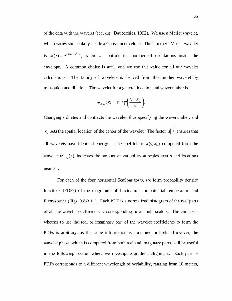
65

of the data with the wavelet (see, e.g., Daubechies, 1992). We use a Morlet wavelet,

which varies sinusoidally inside a Gaussian envelope. The “mother” Morlet wavelet

is 2/2 2

)( ximxex −= πψ , where m controls the number of oscillations inside the

envelope. A common choice is m=1, and we use this value for all our wavelet

calculations. The family of wavelets is derived from this mother wavelet by

translation and dilation. The wavelet for a general location and wavenumber is

⎟⎠⎞

⎜⎝⎛ −

= −

sxx

sxxs02

1

, )(0

ψψ .

Changing s dilates and contracts the wavelet, thus specifying the wavenumber, and

sets the spatial location of the center of the wavelet. The factor 0x 21

−s ensures that

all wavelets have identical energy. The coefficient computed from the

wavelet

),( 0xsw

)(0, xxsψ indicates the amount of variability at scales near s and locations

near . 0x

For each of the four horizontal SeaSoar tows, we form probability density

functions (PDFs) of the magnitude of fluctuations in potential temperature and

fluorescence (Figs. 3.8-3.11). Each PDF is a normalized histogram of the real parts

of all the wavelet coefficients w corresponding to a single scale s. The choice of

whether to use the real or imaginary part of the wavelet coefficients to form the

PDFs is arbitrary, as the same information is contained in both. However, the

wavelet phase, which is computed from both real and imaginary parts, will be useful

in the following section where we investigate gradient alignment. Each pair of

PDFs corresponds to a different wavelength of variability, ranging from 10 meters,

66

which is approaching the Nyquist wavelength (twice the distance between sampling

points, and thus the shortest resolvable wavelength), to 10 kilometers, above which

there are too few independent realizations to yield a PDF with smooth, well-defined

tails. The shape of a PDF at a given spatial scale indicates the frequency with which

fluctuations of various magnitudes occur on that scale. The abscissa is standard

deviations of the real parts of all the wavelet coefficients that form each PDF, so

that the PDFs of fluctuations on small and large scales have equal apparent widths

despite the larger fluctuations that occur on larger scales.

Many studies have attempted to determine the scales at which the horizontal

distribution of chlorophyll is controlled by physical mechanisms by a comparison of

the spectral slope of chlorophyll fluorescence with that of conservative tracers.

Similar spectral slopes are cited as evidence of control by similar mechanisms.

Martin (2003) provides a recent review of such studies. PDF shape, in combination

with spectral information, provides a more stringent test of statistical equivalence of

distinct tracers than does spectral slope alone, and this is our motivation for

examining the scale-specific PDFs of fluctuations in temperature and fluorescence.

At the smallest scales, the PDFs of fluorescence fluctuations are drawn in

dashed lines because their Gaussian shape is the result of instrumental noise. The

temperature PDFs at these small scales have a stretched exponential shape, familiar

from distributions of small-scale scalar difference of a passive scalar in a turbulent

field (e.g. Warhaft, 2000). On the largest scales, the PDFs of potential temperature

and fluorescence fluctuations appear to be converging toward a common

exponential shape.

67

The potential temperature PDFs for the 200-dbar isobar tow (Fig. 3.8) have a

more rounded central peak than those for the 25.5 kg/m3 isopycnal (Fig. 3.10),

indicating less intermittency for small-magnitude events on the isobar. The

difference, though present at all scales, is most noticeable in a length scale range

near 1 kilometer (see the 1280-meter PDFs). The roundness of the temperature

PDFs on the isobar is consistent with variability driven largely by internal waves

having a Gaussian-like distribution (see Briscoe (1977) for a discussion of the

Gaussianity of internal wave vertical displacement). Note also that both the

potential temperature and the fluorescence PDFs on the shallower tows (the 50-dbar

isobar and the 24.8 kg/m3 isopycnal—Figs. 9 and 11 respectively) tend to be more

peaked than those on the deep tows, pointing to a high degree of intermittency (i.e. a

relatively small number of isolated fronts) within the mixed layer.

Of the four horizontal tows, the 50-dbar isobar tow provides the least

contaminated view of small-scale variability in fluorescence. On the deep tows,

instrumental noise competes with the weak fluorescence signal and obscures the true

shape of the small-scale fluorescence PDFs. On the 24.8 kg/m3 isopycnal tow, the

measured small-scale variability in fluorescence is due partly to small deviations

from the target isopycnal in regions where the vertical gradient of chlorophyll

concentration is strong. On the 50-dbar tow, which is comparatively free of both

these complications, the PDFs of fluorescence on scales below a kilometer but

above 100 meters (where the effects of instrumental noise become important), are

rounder than those of temperature (Fig. 3.9). Temperature appears to be more

intermittent than fluorescence on the 50 dbar tow.

68

To summarize, then, at large scales the PDFs of fluctuations in temperature

and fluorescence are similar: by a scale of 10 km (the bottom pair of PDFs in Figs.

3.8-3.11) the temperature and fluorescence PDFs are essentially identical. At the

smallest scales, the true shape of the fluorescence PDFs is obscured by instrumental

noise, but at intermediate scales, there appear to be meaningful differences between

the shapes of temperature and fluorescence PDFs, particularly within the mixed

layer. At these scales, then, different processes may be important in setting the

temperature and fluorescence distributions.

One possible reason for the enhanced intermittency of temperature relative

to fluorescence observed in the PDFs from the 50 dbar isobar is vertical mixing

coupled with gravity-driven slumping of horizontal density gradients in the mixed

layer (e.g. Ferrari and Rudnick, 2000). In a hypothetical mixed layer with initially

random horizontal distributions of temperature and salinity, many of the small-scale

horizontal fluctuations in temperature would be smoothed by vertical mixing as

warm water from one side of a front flowed over cool, denser water from the other.

Only those horizontal temperature fluctuations that were density-compensated by

corresponding salinity fluctuations would persist. The horizontal distribution of

temperature could in this way become more intermittent while that of chlorophyll

fluorescence, a passive tracer, would be less strongly affected.

A second possible explanation of the relative peakiness of the temperature

PDFs is that biological processes are important in determining the small-scale

properties of the horizontal distribution of chlorophyll. For example, it is possible

that unusually large fluctuations in phytoplankton concentration attract grazers,

69

which could then act to eliminate these large fluctuations, reducing the intermittency

of the phytoplankton distribution.

3.4 Temperature-Fluorescence Relationship

To which length scales does the gradient alignment mechanism of Section

3.2 apply? At the smallest scales, the alignment is wiped out by molecular

diffusion, which erases the ‘memory’ of the initial tracer field. As significant

contraction can occur only on scales small relative to the size of the basin, the range

of scales on which alignment might occur is bounded above and below. But the

alignment we actually observe occurs over a narrower range than that. It is difficult

to distinguish on which scales gradients are aligned by simply looking at the records

(see Figs. 3.2-3.5). The wavelet coefficients from Section 3.3 can help resolve this

issue. Associated with each wavelet coefficient w is a phase

⎟⎟⎠

⎞⎜⎜⎝

⎛= −

)Re()Im(tan 1

wwφ .

At a given scale and location we can define the temperature-fluorescence phase

difference as ),(),(),( sxsxsx fφφφ θ −=Δ , where θφ and fφ refer to potential

temperature and fluorescence respectively. Fluorescence-temperature gradient

alignment is indicated by values of φΔ near zero (in phase) and π± (out of phase).

Peaks at zero and π± in the PDF of φΔ at a given length scale s are thus an

indication of a tendency for temperature and fluorescence gradients to align on that

scale.

70

Figure 3.12 shows the distribution of wavelet phase difference for the 200-

dbar isobar tow. PDFs of φΔ for scales ranging from 1 km to 100 km are stacked

together from front to back. The alignment is almost exclusively in-phase because

the variability along that surface is dominated by vertical displacements, and the

vertical gradients are of unchanging sign (see Fig. 3.1). The relationship weakens at

smaller scales, but remains evident all the way down to a kilometer.

On scales of 10 km and above, the alignment between temperature and

fluorescence on the 50-dbar tow is predominantly in-phase (Fig. 3.13). This large-

scale alignment is confined mainly to the northern end of the tow, and is directly

visible in Fig. 3.3. As discussed in Section 3.2, the alignment is probably caused by

stirring. At scales smaller than 10 km, temperature and fluorescence are aligned

out-of-phase, a relationship which holds throughout the tow, but is strongest in the

southern part. At these scales, both temperature and fluorescence are strongly

correlated with measured density, suggesting that the small-scale alignment is the

result of diapycnal profiling. The correlation between pressure and both temperature

and fluorescence is very weak, however. Thus, the diapycnal profiling is caused not

by deviations in SeaSoar’s flight path, but by vertical displacement of water by

internal waves.

On the 25.5 kg/m3 isopycnal tow, in-phase gradient alignment is evident at

scales of 10 km and above (Fig. 3.14). Out-of-phase alignment is evident on the

largest scales as well, though less strongly because only a quarter of the section

(Fig. 3.4) was aligned out of phase. Like the large-scale alignment at 50 dbar, this

relationship is well explained by stirring-enhanced gradients.

71

Alignment is not obvious at the larger scales on the 24.8 kg/m3 isopycnal

tow (Fig. 3.15), but some alignment, mainly in-phase, is evident at scales of 1 km

and smaller. At these scales, fluctuations in density are aligned with those in both

temperature and fluorescence. This suggests that the observed small-scale

alignment between temperature and fluorescence is the result of unintentional

diapycnal profiling, demonstrating that the corrections made for deviation from the

isopycnal are not perfect.

To summarize, then, the alignment that we attribute to gradient enhancement

by stirring (namely, that on the 25.5 kg/m3 isopycnal and the in-phase alignment at

50 dbar), disappears below a scale of 10 km. Smaller-scale alignment, observed

most strongly on the 50 dbar tow but also on the 200 dbar and 24.8 kg/m3 isopycnal

tows, is likely the result of diapycnal profiling.

3.5 Renovating Wave Model

Plankton ecosystem models with simple representations of turbulent stirring

can reproduce the power-law spectra typical of oceanic fluorescence measurements

(e.g. Abraham, 1998). We explore the effect of such stirring on tracer gradient

alignment with a simple Lagrangian advection model, which has been dubbed

(William Young, pers. commun.) the ‘renovating wave’ (hereafter RW) model.

This model was originally used in dynamo theory (see e.g. Childress and Gilbert,

1995), and similar formulations have found use in the study of turbulence

(Pierrehumbert, 1994) and plankton patchiness (Young et al., 2001). The model

consists of sinusoidal shear flows, which are periodically renovated by the choice of

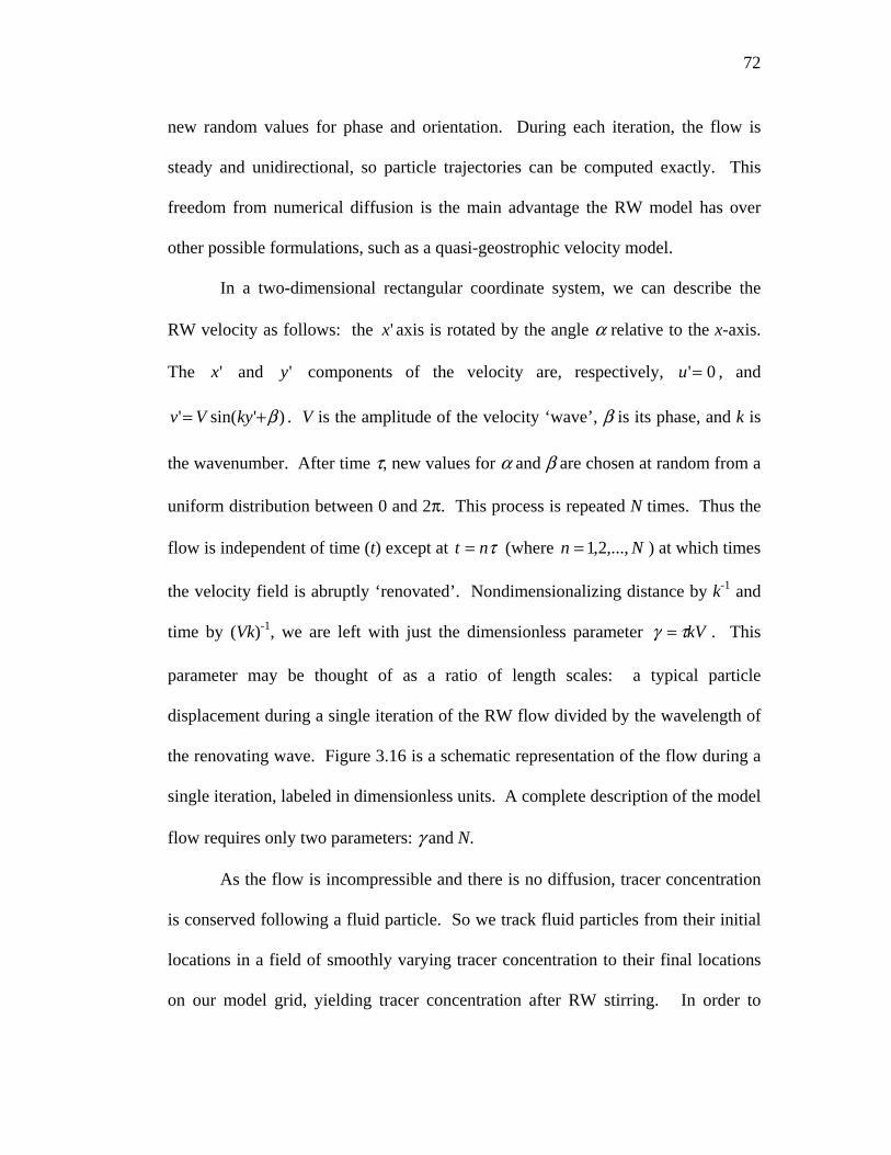
72

new random values for phase and orientation. During each iteration, the flow is

steady and unidirectional, so particle trajectories can be computed exactly. This

freedom from numerical diffusion is the main advantage the RW model has over

other possible formulations, such as a quasi-geostrophic velocity model.

In a two-dimensional rectangular coordinate system, we can describe the

RW velocity as follows: the axis is rotated by the angle α relative to the x-axis.

The and components of the velocity are, respectively, , and

'x

'x 'y 0'=u

)'sin(' β+= kyVv . V is the amplitude of the velocity ‘wave’, β is its phase, and k is

the wavenumber. After time τ, new values for α and β are chosen at random from a

uniform distribution between 0 and 2π. This process is repeated N times. Thus the

flow is independent of time (t) except at τnt = (where ) at which times

the velocity field is abruptly ‘renovated’. Nondimensionalizing distance by k-1 and

time by (Vk)-1, we are left with just the dimensionless parameter

Nn ,...,2,1=

kVτγ = . This

parameter may be thought of as a ratio of length scales: a typical particle

displacement during a single iteration of the RW flow divided by the wavelength of

the renovating wave. Figure 3.16 is a schematic representation of the flow during a

single iteration, labeled in dimensionless units. A complete description of the model

flow requires only two parameters: γ and N.

As the flow is incompressible and there is no diffusion, tracer concentration

is conserved following a fluid particle. So we track fluid particles from their initial

locations in a field of smoothly varying tracer concentration to their final locations

on our model grid, yielding tracer concentration after RW stirring. In order to

73

avoid the necessity of interpolating particle positions onto a grid and the associated

imprecision, we employ the following trick: the final particle positions are chosen

to coincide exactly with a grid, and the model is run backward in time to obtain the

initial particle positions. We specify tracer concentration as a function of these

initial positions. Perhaps the simplest non-constant function possible is a planar

initial concentration field (uniform initial concentration gradient), and all the

simulations included in the present study use this choice.

When two tracer fields, initially uncorrelated, are stirred by the same RW

flow, similar features develop in both fields (Fig. 3.17). In this example, the initial

tracer concentration gradient was uniform and of equal magnitude in each case, but

initial gradient direction differed by 90 degrees. The number of iterations, N, is 70,

and γ is 0.8. The size of the domain pictured, in units of k-1, is 2π; that is, one

complete RW wave would fit along each side of the box. In some locations, high-

concentration features in one field correspond to low-concentration features in the

other (out-of-phase gradient alignment), while in others, corresponding features in

the two fields are either both high- or both low-concentration (in-phase gradient

alignment). In the Appendix to this chapter we show that, for the case just

described, the alignment of tracer gradients is inevitable. This mechanism is likely

responsible for the alignment observed on the 25.5 kg/m3 isopycnal.

PDFs of wavelet phase differences for two tracers stirred by the RW process

that produced the fields in Fig. 3.17 are sharply peaked around 0=θ and πθ =

(Fig. 3.18). Thus, the stirred fields exhibit both in-phase and out-of-phase

alignment at all scales. Potential temperature and chlorophyll on the 25.5 kg/m3

74

isopycnal (Fig. 3.14) and the 50-dbar isobar (Fig. 3.13) were aligned on large scales,

but in both cases, the alignment faded out at a length-scale of ~10 km (as discussed

in Section 3.4, the small-scale, out-of-phase alignment on the 50-dbar tow was

caused by internal waves). If stirring caused the alignment we observed, we would

like to understand what prevented alignment on scales smaller than 10 km.

One possibility is that small-scale gradient alignment is destroyed by mixing.

In the irreversible process of turbulent diffusion, memory of the initial field is lost—

narrow tracer filaments that would be aligned are simply mixed out of existence.

Turbulent diffusion may be included in the RW model by introducing independent

random displacements along with the RW advection velocity at each time-step.

These diffusive displacements are meant to reflect the combined effect of all the

turbulent motions on scales smaller than the grid scale (the large-scale motion being

our prescribed RW flow), so there is no correlation between the displacements

experienced by neighboring particles. We use normally distributed, isotropic

diffusive displacements, with a RMS magnitude of D. In the absence of advection,

this corresponds to a diffusion coefficient, κ, of 1221 −τD . Defining kD=δ , the

model now contains two nondimensional parameters: γ describes the

nondimensional distance moved at each iteration due to advection, and δ the

nondimensional distance moved due to turbulent motions. The ratio of diffusive to

advective timescales is the Peclet number, . 2/Pe δγ=

A single realization of the RW process with diffusive displacements causes

local scattering of fluid particles and so produces a ‘speckled’ field (Fig. 3.19, left

75

panel). Here the initial concentration field and RW stirring sequence are identical to

those in Fig. 3.17, left panel, but we have included diffusive displacements, with

024.0=δ . If the grid is regarded as a pixelation of the fluid, then the

concentrations we thus obtain represent the concentration at the initial location of

one infinitesimal point in each pixel. Another tiny fluid particle in the same pixel

would in general have a different initial location and concentration. Rather than the

concentration at a single particle, we would like a representative concentration for

the entire pixel. Accordingly, we run the model a large number of times (here, 100)

with identical RW stirring but independent diffusive displacements. The

concentration assigned to a pixel is then the mean concentration at that pixel over

the ensemble, which we can think of as the average concentration over the ‘box’ of

fluid represented by the pixel. The assumption is that the RW wavelength is large

compared to the grid scale, so that the advecting velocity is essentially constant over

each pixel, and that the grid scale is large compared to the diffusion velocity

decorrelation length scale, so that the diffusive displacements of the particles which

end up scattered throughout that pixel are unrelated. The ensemble average

concentration field after RW advection with diffusion is shown in Fig. 3.19, right

panel.

In order to investigate the effect of diffusion on gradient alignment in the

RW model, we follow the procedure described above to stir and mix two tracer

fields with distinct initial conditions. As in Fig. 3.18, the two tracers are stirred by

the same RW flow, but now each of the tracers is subject to its own set of random

diffusive displacements. This is tantamount to choosing, for each tracer, a unique,

76

random set of 100 fluid particles within each pixel from which to form the ensemble

average. Using the identical set of diffusive displacements for each tracer (that is,

using the same set of fluid particles) would introduce artificial correlations between

the two fields—any inhomogeneity in the distribution of diffusive displacements in

a pixel would cause a similar bias in each of the two fields.

Our two stirred tracer fields still show gradient alignment at scales above 0.1

(nondimensional distance), but the peaks in the wavelet phase difference PDFs

vanish at smaller scales (Fig. 3.20). The parameters are the ones used in Fig. 3.19:

N=70, γ =0.8, and δ=0.024. As an example of the level of horizontal mixing

required in the ocean to erase small-scale gradient alignment, we can choose values

for dimensional model parameters. Setting m-1 (so that the RW wavelength

or typical ‘eddy’ size is ~60 km), the model cutoff length scale of approximately 0.1

corresponds to the observed cutoff length scale of approximately 10 km. Choosing

a maximum current velocity V of 0.1 m/s, the time between renovations, τ, is

s, or roughly one day, and D, the typical diffusive displacement per

renovation, is 240 m. The diffusion coefficient, κ, is then 0.36 m2/s, roughly

comparable with measurements of open-ocean horizontal eddy diffusivity on 1-10

km scales (Ledwell et al., 1998).

410−=k

4108×

The result of small-scale turbulence (the ‘diffusive displacements’ in our

model) and mixing (the averaging of an ensemble of particles in each pixel) is thus

to suppress gradient alignment at small scales. Turbulent mixing, then, is one

possible explanation for the deterioration of gradient alignment observed at small

scales on isopycnals.

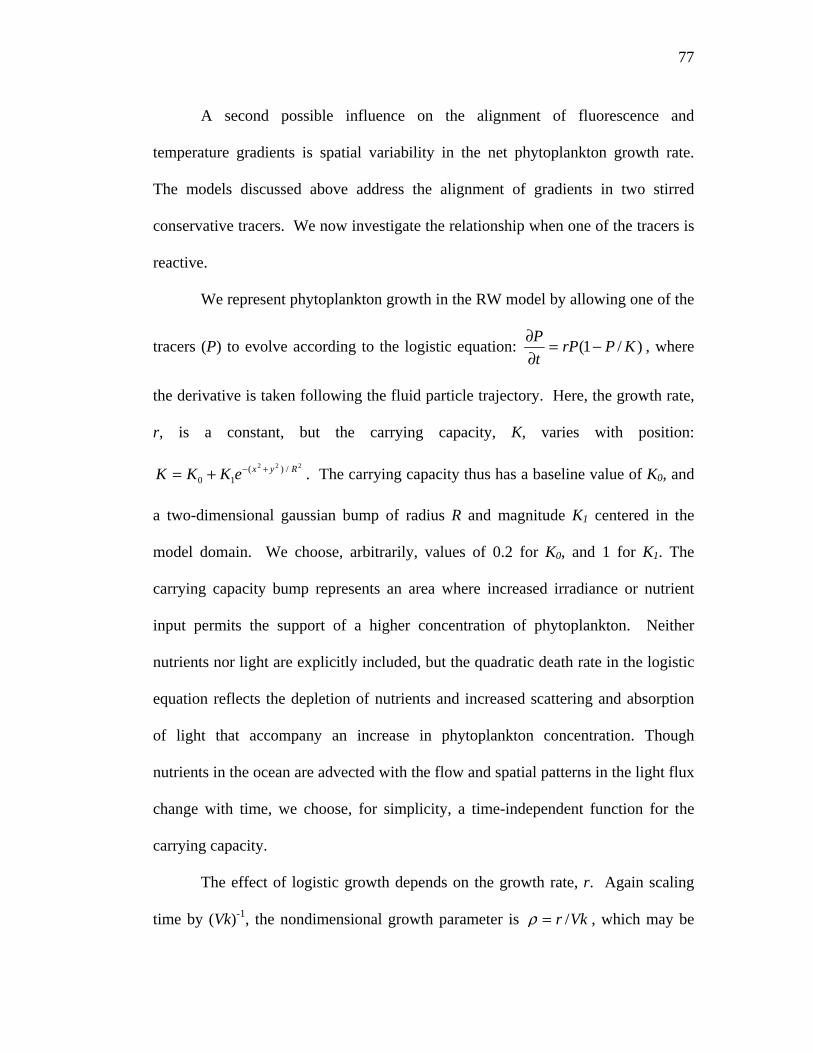
77

A second possible influence on the alignment of fluorescence and

temperature gradients is spatial variability in the net phytoplankton growth rate.

The models discussed above address the alignment of gradients in two stirred

conservative tracers. We now investigate the relationship when one of the tracers is

reactive.

We represent phytoplankton growth in the RW model by allowing one of the

tracers (P) to evolve according to the logistic equation: )/1( KPrPtP −=

∂∂ , where

the derivative is taken following the fluid particle trajectory. Here, the growth rate,

r, is a constant, but the carrying capacity, K, varies with position:

. The carrying capacity thus has a baseline value of K0, and

a two-dimensional gaussian bump of radius R and magnitude K1 centered in the

model domain. We choose, arbitrarily, values of 0.2 for K0, and 1 for K1. The

carrying capacity bump represents an area where increased irradiance or nutrient

input permits the support of a higher concentration of phytoplankton. Neither

nutrients nor light are explicitly included, but the quadratic death rate in the logistic

equation reflects the depletion of nutrients and increased scattering and absorption

of light that accompany an increase in phytoplankton concentration. Though

nutrients in the ocean are advected with the flow and spatial patterns in the light flux

change with time, we choose, for simplicity, a time-independent function for the

carrying capacity.

222 /)(10

RyxeKKK +−+=

The effect of logistic growth depends on the growth rate, r. Again scaling

time by (Vk)-1, the nondimensional growth parameter is Vkr /=ρ , which may be

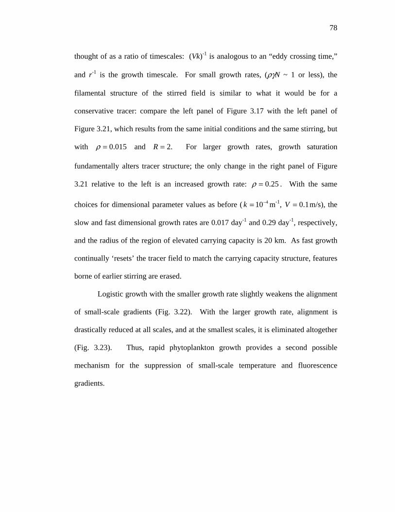
78

thought of as a ratio of timescales: (Vk)-1 is analogous to an “eddy crossing time,”

and r-1 is the growth timescale. For small growth rates, (ργN ~ 1 or less), the

filamental structure of the stirred field is similar to what it would be for a

conservative tracer: compare the left panel of Figure 3.17 with the left panel of

Figure 3.21, which results from the same initial conditions and the same stirring, but

with 015.0=ρ and For larger growth rates, growth saturation

fundamentally alters tracer structure; the only change in the right panel of Figure

3.21 relative to the left is an increased growth rate:

.2=R

25.0=ρ . With the same

choices for dimensional parameter values as before ( m-1, m/s), the

slow and fast dimensional growth rates are 0.017 day-1 and 0.29 day-1, respectively,

and the radius of the region of elevated carrying capacity is 20 km. As fast growth

continually ‘resets’ the tracer field to match the carrying capacity structure, features

borne of earlier stirring are erased.

410−=k 1.0=V

Logistic growth with the smaller growth rate slightly weakens the alignment

of small-scale gradients (Fig. 3.22). With the larger growth rate, alignment is

drastically reduced at all scales, and at the smallest scales, it is eliminated altogether

(Fig. 3.23). Thus, rapid phytoplankton growth provides a second possible

mechanism for the suppression of small-scale temperature and fluorescence

gradients.

79

3.6 Summary and Discussion

The PDFs of scale-specific fluctuations in temperature and fluorescence

(Section 3.3) are very similar to each other for scales of a few kilometers and larger.

With the exception of the 200 dbar tow, on which variability was dominated by

internal waves, fluorescence PDFs for length scales near one kilometer differ in

shape from the corresponding temperature PDFs. On this scale, the horizontal

distribution of temperature on the 50 dbar isobar and the 25.5 kg/m3 isopycnal was

more intermittent than that of fluorescence, while it was less intermittent on the 24.8

kg/m3 isopycnal. The difference suggests that on ~1 km scales, temperature and

fluorescence distributions may be established by distinct mechanisms. At the

smallest scales, such comparisons are precluded by instrumental noise in the

fluorescence data.

The alignment of gradients in potential temperature and chlorophyll

fluorescence on the 25.5 kg/m3 isopycnal, both in-phase and out-of-phase, indicates

that at least at scales of 10-100 km, stirring may well play a dominant role in setting

the along-isopycnal distribution of chlorophyll below the euphotic zone. In-phase

alignment on the 50-dbar tow suggests that stirring can also control the horizontal

chlorophyll distribution at these scales in the euphotic zone and above the mixed

layer base. However, alignment at 10-100 km scales is scarcely evident on the 24.8

kg/m3 isopycnal, demonstrating that stirring is not always the primary influence on

along-isopycnal chlorophyll. The correlation between isopycnal depth and

chlorophyll fluorescence on this tow suggests that locally enhanced growth rates can

be important in determining the chlorophyll distribution.

80

Stirring does not appear to produce much alignment on scales smaller than

10 km. Small-scale alignment on isobars is the result of vertical advection, and the

apparent alignment on the 24.8 kg/m3 isopycnal is caused by deviations of the

instrument package from the isopycnal. Correcting the data for these deviations

reduces the strength of the alignment, but as a perfect correction is impossible, some

leftover alignment is inevitable.

We have employed a renovating wave model to demonstrate the alignment

of gradients in stirred tracers, and to investigate possible reasons for the lack of

alignment at scales smaller than the observed cutoff length scale of approximately

10 km. The model suggests that both turbulent mixing and phytoplankton growth

could weaken small-scale gradient alignment. In our model with logistic growth

and a spatially varying carrying capacity, only growth with a time-scale short in

comparison with the duration of the advecting flow is effective in suppressing

gradient alignment. A search of N-γ-δ parameter space reveals that the cutoff length

scale, L, below which gradient alignment is destroyed by diffusion in the RW model

increases with increasing δ, and decreases with increasing N and γ.

The relationship between δ and L can be verified for any value of δ small

compared to one, but N and γ cannot independently be varied over a very large

dynamic range. Gradient alignment only occurs if the cumulative effect of the RW

stirring has been to produce highly strained regions in the fluid. If either N or γ is

too small, this condition is not satisfied. On the other hand, if either N or γ is too

large, the strain is so extreme that initially distant fluid particles (i.e., particles

whose separation is comparable to the RW wavelength) approach closer than the

81

model grid spacing, the tracer filaments become too narrow to be resolved, and the

smoothly varying character of the tracer field is lost.

Consider an infinitesimal material line element of length l at the origin,

oriented along the y-axis in Fig. 3.16. In the coordinate system, this material

line element is represented as a vector:

'x 'y

)cos,(sin ααl . After being advected by the

first iteration of the RW flow, the material line element has been stretched, and

becomes )sincoscos,(sin αβγαα +l . The squared length of the material line

element is now . Both α and β are

uniformly distributed between 0 and 2π, so the expectation value of the square of

the elongation factor E of a small random material line element during a single RW

iteration is

]sincoscossincos21[ 2222 αβγααβγ ++l

2412 1 γ+=E . Provided that the line element stays short compared to

the RW wavelength, we can thus describe the elongation after N iterations as

( ) 22412 1

NNE γ+= , which is a measure of the total strain. If we denote the ratio

of the RW wavelength to the gridscale by R, then the strain condition for the

occurrence of gradient alignment becomes ( ) RN

<<+<< 224111 γ . As a

dimensional example, if we retain the parameter choices from Section 3.5

( m-1, m/s, s), the lower bound on the time required for

gradient alignment to develop is on the order of a month.

410−=k 1.0=V 4108×=τ

Within the region of parameter space where we observe gradient alignment

( ( ) RN

<<+<< 224111 γ ), increasing strain pushes the lower bound L of the gradient

alignment length scale toward smaller values, and increasing diffusion does the

82

opposite. While the growth of L with δ is intuitive, it is perhaps a little surprising

that throughout most of parameter space, L is several times larger than δ. Adding

diffusion to the RW model eliminates gradient alignment at scales larger than the

individual diffusive displacements. To two neighboring fluid particles whose

separation is small compared to the RW wavelength, the RW flow looks like a linear

shear flow with a periodically changing direction. In this regime, the distance

between the two particles grows exponentially in time, which is the expected

behavior of nearby particles in real turbulent flows (Batchelor, 1952). One

consequence of this is that perturbing a particle’s location by introducing a small

diffusive displacement can have a comparatively large effect on where the particle

ends up several RW iterations later. This ‘butterfly effect’ helps explain how

seemingly small displacements can wipe out tracer filaments and erode gradient

alignment at scales larger than the displacements themselves.

There are many choices besides the Morlet wavelet transform for analyzing

spatial distributions from data collected along a line. One popular alternative

statistic is the so-called scalar difference (e.g. Warhaft, 2000). For a scalar S, (say

temperature), the scalar difference is defined as . Here, d is the

separation between a pair of points, and is the difference in S between the

two. For any values of d we choose, we can take all pairs of points in the record

separated by d, and plot probability density functions of the scalar differences. A

PDF with long tails indicates intermittent behavior, while sharply dropping tails

imply relative uniformity.

2/12)(/)( ⟩Δ⟨Δ dSdS

)(dSΔ

83

The scalar difference may be expressed as a convolution of the scalar S with

a pair of Dirac delta functions: )]()([),( 22dd xxSdxS +−−∗=Δ δδ . Convolution in

physical space is equivalent to multiplication in wavenumber space, so the Fourier

transform of the convolution function reveals the spatial scales of variability to

which the scalar difference statistic is sensitive. The Fourier transform of

)()( 22dd xx +−− δδ is , where k is the wavenumber. The magnitude of

the Fourier transform reaches a maximum at

)2/sin(2 kdi

dk /π= , corresponding to variability

with a semi-wavelength of d. There are also maxima in the magnitude at dnk /π=

for all odd integers n. If the goal is to understand the degree of intermittency of the

field as a function of spatial scale, it is desirable to treat each scale separately, rather

than using a method of analysis that folds variability at multiple scales into a single

statistic. In most situations, the spectrum of tracers is decidedly red—that is, there

is more variability at longer length scales. For this reason, variability at the

fundamental length scale, that is, at a semi-wavelength of d, may dominate the

scalar difference signal. Nonetheless, we chose here to use a mode of analysis that

focuses on each wavenumber band individually. Instead of a pair of delta functions,

we use an analyzing function ψ that is compact in both physical space and

wavenumber.

Large-scale fluid motions, through accumulated strain, produce structure in

tracer fields at much smaller scales. Meanwhile, small-scale turbulent motions

promote mixing, which destroys small-scale tracer structure. We have argued that

the demonstrated alignment of horizontal chlorophyll and temperature gradients is

likely the result of large-scale motions, and suggested turbulent mixing and rapid

84

phytoplankton growth as possible causes of the breakdown of that alignment at

small scales. The role that spatial variability in phytoplankton growth plays in

determining the horizontal distribution of chlorophyll within the euphotic zone is an

important question. Large and variable vertical chlorophyll gradients in this region

make investigation of this issue by analysis of a horizontal tow difficult. During an

April 2005 cruise in the northeastern Pacific, we towed SeaSoar along a sawtooth

track spanning the deep chlorophyll maximum, completing a cycle every 700 meters

over a section 1000 km in length. Future analysis of this dataset and others like it

will further our understanding of the combination of factors controlling chlorophyll

structure in the ocean.

Acknowledgments. We thank Bill Young for introducing us to the

renovating wave model, and three anonymous reviewers for many helpful

comments. We gratefully acknowledge the generous support of the National

Science Foundation (OCE98-19530 and OCE04-52574). Chapter 3, in full, is a

reproduction of the material as it has been submitted to Deep-Sea Research I. The

dissertation author was the primary investigator and author of this paper.

85

Appendix (Chapter 3)

Proof that alignment of stirred tracers with uniform initial gradients is inevitable.

Let u be a two-dimensional incompressible velocity field, so that . 0=⋅∇ u

Let a and b be conservative, nondiffusive tracers subject to advection by u. Then a

and b satisfy the advection equation:

0=∇⋅+∂∂ a

ta u , and 0=∇⋅+

∂∂ b

tb u .

This simply states that a and b are conserved following fluid particle trajectories.

We define the Jacobian of a and b as the cross product of with : a∇ b∇

xb

ya

yb

xabaJ

∂∂

∂∂−

∂∂

∂∂=),( .

Plugging the Jacobian, written in this form, into the advection equation, it is easily

shown that

0),(),( =∇⋅+∂

∂ baJt

baJ u .

Thus, the Jacobian is also conserved following fluid particle trajectories.

The Jacobian can alternately be expressed as

θsin),( babaJ ∇∇= ,

where θ is the angle between and . In the simple case of planar initial

concentration fields, , , and θ are independent of position at time , so

a∇ b∇

a∇ b∇ 0=t

86

kbaJ =),( , where k is a constant. That is, the Jacobian is constant, independent of

position and time. However, as stirring stretches the tracer fields a and b, the large-

time behavior of a∇ and b∇ is to increase without bound (see e.g. Eckart, 1948).

Therefore

kba =∇∇ θsin

requires that

0sin →θ as . ∞→t

Under the influence of stirring, the tracer concentration gradients tend toward

alignment, either in phase ( 0=θ ), or out of phase ( πθ = ).

87

Latitude (°N)

Pre

ssur

e (d

bar)

26 27 28 29 30 31 32 33 34

50

100

150

200

250

300

Fluorescence (V)0.14 0.16 0.18 0.2 0.22 0.24 0.26

Figure 3.1. Fluorescence section with isobar and isopycnal tows drawn in white. Black lines are 0.1 kg/m3 density contours. The jagged white lines do not coincide with the black density contours because by the time the isopycnal tows were carried out, the isopycnals had moved. In terms of chlorophyll concentration, the color scale runs roughly from 0 to 2 mg/m3.

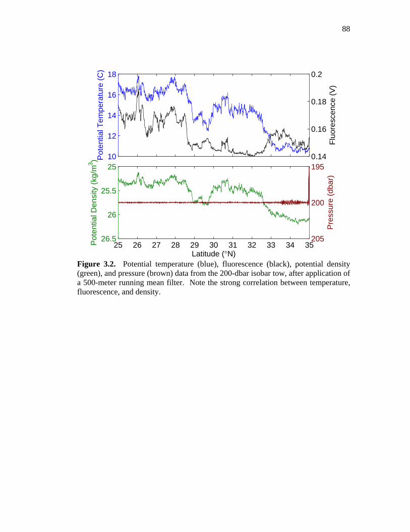
88

10

12

14

16

18

Pot

entia

l Tem

pera

ture

(C

)

0.14

0.16

0.18

0.2

Flu

ores

cenc

e (V

)

25 26 27 28 29 30 31 32 33 34 35

25

25.5

26

26.5Pot

entia

l Den

sity

(kg

/m3 )

Latitude (°N)

195

200

205

Pre

ssur

e (d

bar)

Figure 3.2. Potential temperature (blue), fluorescence (black), potential density (green), and pressure (brown) data from the 200-dbar isobar tow, after application of a 500-meter running mean filter. Note the strong correlation between temperature, fluorescence, and density.

89

16

18

20

22

Pot

entia

l Tem

pera

ture

(C

)

0.14

0.16

0.18

0.2

0.22

0.24

Flu

ores

cenc

e (V

)

25 26 27 28 29 30 31 32 33 34 35

24.5

24.6

24.7

24.8

24.9

25Pot

entia

l Den

sity

(kg

/m3 )

Latitude (°N)

45

50

55

Pre

ssur

e (d

bar)

Figure 3.3. Data from the 50-dbar isobar tow, plotted as in Fig. 3.2. Temperature and fluorescence are strongly correlated in the northern portion of the tow.

90

12

13

14

15

16

Pot

entia

l Tem

pera

ture

(C

)

0.14

0.16

0.18

0.2

Flu

ores

cenc

e (V

)

25 26 27 28 29 30 31 32 33 34 35

25.4

25.5

25.6Pot

entia

l Den

sity

(kg

/m3 )

Latitude (°N)

100

150

200

250

Pre

ssur

e (d

bar)

Figure 3.4. Data from the 25.5 kg/m3 isopycnal tow, plotted as in Fig. 3.2. Near 32° N the temperature-fluorescence relationship switches from in-phase to out-of-phase.

91

19

20

21

Pot

entia

l Tem

pera

ture

(C

)

0.15

0.2

0.25

0.3

Flu

ores

cenc

e (V

)

25 26 27 28 29 30 31 32

24.7

24.8

24.9Pot

entia

l Den

sity

(kg

/m3 )

Latitude (°N)

0

50

100

150

200

Pre

ssur

e (d

bar)

Figure 3.5. Data from the 24.8 kg/m3 isopycnal tow, plotted as in Fig. 3.2. The correlation between pressure and fluorescence in the southern part of the tow indicates the stimulation of algal growth by the increase in irradiance produced by uplift of the isopycnal.

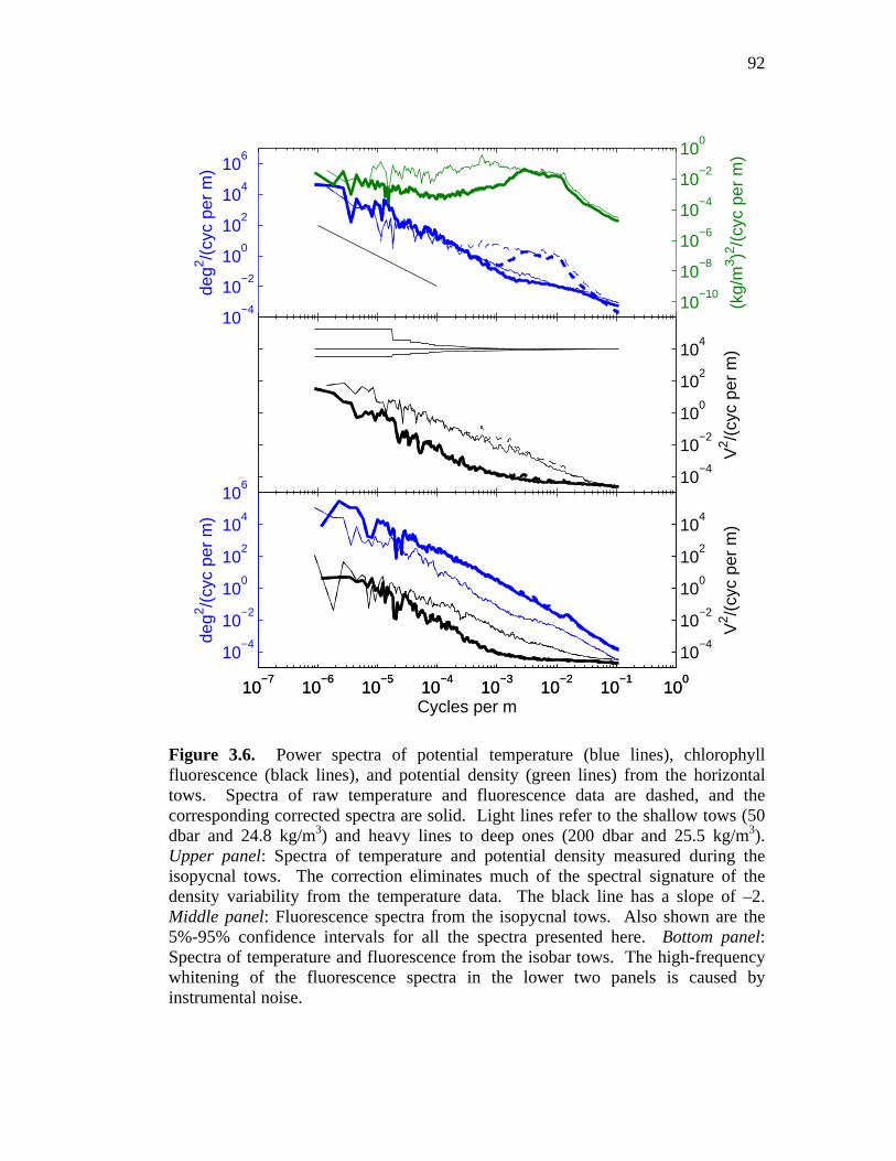
92

10−4

10−2

100

102

104

106

deg2 /(

cyc

per

m)

10−10

10−8

10−6

10−4

10−2

100

(kg/

m3 )2 /(

cyc

per

m)

10−4

10−2

100

102

104

V2 /(

cyc

per

m)

10−7

10−6

10−5

10−4

10−3

10−2

10−1

100

10−4

10−2

100

102

104

106

deg2 /(

cyc

per

m)

10−7

10−6

10−5

10−4

10−3

10−2

10−1

100

10−4

10−2

100

102

104

V2 /(

cyc

per

m)

Cycles per m

Figure 3.6. Power spectra of potential temperature (blue lines), chlorophyll fluorescence (black lines), and potential density (green lines) from the horizontal tows. Spectra of raw temperature and fluorescence data are dashed, and the corresponding corrected spectra are solid. Light lines refer to the shallow tows (50 dbar and 24.8 kg/m3) and heavy lines to deep ones (200 dbar and 25.5 kg/m3). Upper panel: Spectra of temperature and potential density measured during the isopycnal tows. The correction eliminates much of the spectral signature of the density variability from the temperature data. The black line has a slope of –2. Middle panel: Fluorescence spectra from the isopycnal tows. Also shown are the 5%-95% confidence intervals for all the spectra presented here. Bottom panel: Spectra of temperature and fluorescence from the isobar tows. The high-frequency whitening of the fluorescence spectra in the lower two panels is caused by instrumental noise.

93

24.7

24.75

24.8

24.85

24.9

σ θ (kg

/m3 )

18 20 22 24 26 28 30 32 34 36

0

50

100

150

Latitude (minutes north of 29°N)

Pre

ssur

e (d

bar)

Flu

ores

cenc

e (V

)

0.18

0.19

0.2

0.21

0.22

0.23

0.24

0.25

0.26

0.27

Figure 3.7. Upper panel: Potential density measurements, averaged to 1 Hz, from a short section of the 24.8 kg/m3 isopycnal tow where deviations from the isopycnal were particularly severe. The color of each point indicates chlorophyll fluorescence, showing that the oscillations spanned the deep chlorophyll maximum. Lower panel: Same as above, but with pressure as the vertical axis.

94

−6 −4 −2 0 2 4 6

10−20

10−15

10−10

10−5

100

10 m

20 m

40 m

80 m

160 m

320 m

640 m

1280 m

2560 m

5120 m

10240 m

Fluctuation Magnitude (std devs)

PD

F200 dbar

Figure 3.8. PDFs of potential temperature (blue) and fluorescence (black) wavelet coefficients on the 200-dbar isobar tow, showing the distribution of the magnitude of fluctuations in these tracers at each of 11 logarithmically-spaced scales (wavelengths). Each pair of PDFs is labeled with its wavelength, and displaced by two orders of magnitude from the pair above it. Small-scale fluorescence PDFs are dashed to indicate the influence of instrumental noise.

95

−6 −4 −2 0 2 4 6

10−20

10−15

10−10

10−5

100

10 m

20 m

40 m

80 m

160 m

320 m

640 m

1280 m

2560 m

5120 m

10240 m

Fluctuation Magnitude (std devs)

PD

F50 dbar

Figure 3.9. PDFs of temperature and fluorescence wavelet coefficients on the 50-dbar isobar tow, plotted as in Fig. 3.8.

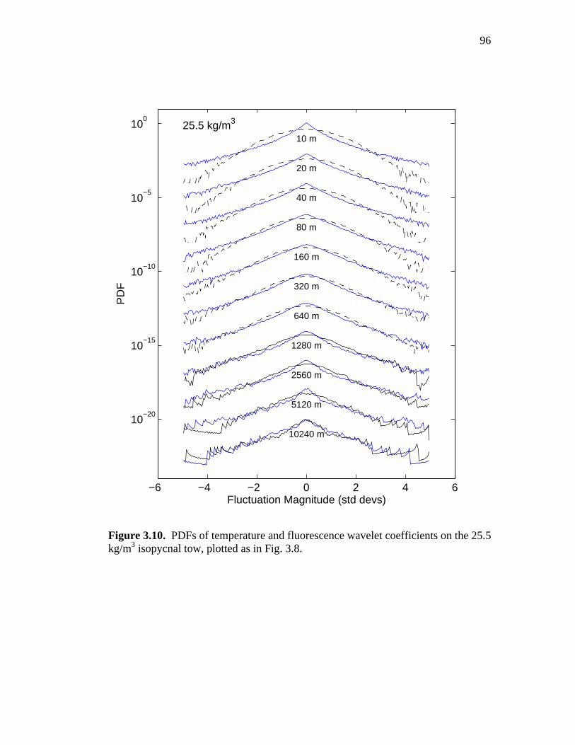
96

−6 −4 −2 0 2 4 6

10−20

10−15

10−10

10−5

100

10 m

20 m

40 m

80 m

160 m

320 m

640 m

1280 m

2560 m

5120 m

10240 m

Fluctuation Magnitude (std devs)

PD

F25.5 kg/m3

Figure 3.10. PDFs of temperature and fluorescence wavelet coefficients on the 25.5 kg/m3 isopycnal tow, plotted as in Fig. 3.8.

97

−6 −4 −2 0 2 4 6

10−20

10−15

10−10

10−5

100

10 m

20 m

40 m

80 m

160 m

320 m

640 m

1280 m

2560 m

5120 m

10240 m

Fluctuation Magnitude (std devs)

PD

F24.8 kg/m3

Figure 3.11. PDFs of temperature and fluorescence wavelet coefficients on the 24.8 kg/m3 isopycnal tow, plotted as in Fig. 3.8.

98

−π0

π

1

10

1000

0.5

1

1.5

Phase differenceScale (km)

PDF

Figure 3.12. PDFs, plotted as bar graphs, of phase difference between temperature and fluorescence wavelet coefficients on the 200-dbar isobar. The color of each bar corresponds to its height, and spatial scale increases from front to back. The peak at a phase difference of zero indicates in-phase alignment of gradients, which is stronger at larger scales.

99

−π0

π

0.1

1

10

1000

0.5

1

1.5

Phase differenceScale (km)

PDF

Figure 3.13. As in Fig. 3.12, for wavelet coefficients on the 50-dbar isobar. Gradients are aligned in-phase at large scales and out of phase (peaks at ± π) at small scales.

100

−π0

π

1

10

1000

0.5

1

1.5

Phase differenceScale (km)

PDF

Figure 3.14. As in Fig. 3.12, for wavelet coefficients on the 25.5 kg/m3 isopycnal. Large-scale alignment is evident both in-phase and (more weakly) out-of-phase.

101

−π0

π

0.1

1

10

1000

0.5

1

1.5

Phase differenceScale (km)

PDF

Figure 3.15. As in Fig. 3.12, for wavelet coefficients on the 24.8 kg/m3 isopycnal. Small-scale alignment is the result of unintentional deviations from the isopycnal.

102

x

y

β

2π

γ

α

Figure 3.16. Velocity during a single iteration of the RW model flow. α is the angle or orientation of the renovating wave, β is its phase, and γ is the nondimensional amplitude (maximum particle displacement relative to the RW wavelength).

103

−π 0 π−π

0

π

−π 0 π−π

0

π

Figure 3.17. Two tracer fields stirred by an identical RW flow. γ is 0.8 and the number of iterations, N, is 70. Initial concentration gradients were uniform and equal in each case, but gradient direction differed by 90 degrees. Corresponding features in each panel are obvious; in some locations, the fields are in phase with each other, while in others they are out of phase.

104

−π

0

π

0.01

0.1

10

0.05

0.1

0.15

0.2

0.25

Phase difference

Spatial scale

PDF

Figure 3.18. PDFs of phase differences, plotted as in Fig. 3.12, between wavelet coefficients for two tracer fields stirred by the same RW flow, showing both in-phase and out-of-phase alignment at all scales. As is Fig. 3.17, γ is 0.8 and N is 70.

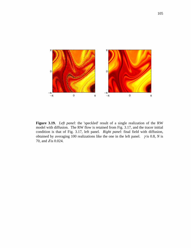
105

−π 0 π−π

0

π

−π 0 π−π

0

π

Figure 3.19. Left panel: the 'speckled' result of a single realization of the RW model with diffusion. The RW flow is retained from Fig. 3.17, and the tracer initial condition is that of Fig. 3.17, left panel. Right panel: final field with diffusion, obtained by averaging 100 realizations like the one in the left panel. γ is 0.8, N is 70, and δ is 0.024.

106

−π

0

π

0.01

0.1

10

0.05

0.1

0.15

0.2

0.25

Phase difference

Spatial scale

PDF

Figure 3.20. As in Fig. 3.18, for wavelet coefficients for two tracers stirred by the same RW flow, with turbulent diffusion. Alignment is suppressed below a spatial scale of 0.1. As in Fig. 3.19, γ is 0.8, N is 70, and δ is 0.024.

107

−π 0 π−π

0

π

−π 0 π−π

0

π

Figure 3.21. Reactive tracers subject to logistic growth. The RW flow is the same as in the earlier figures, and the initial condition is that of Fig. 3.17, left panel. The radius of the carrying capacity bump, R, is 2. Growth rate parameters for the two fields are (left panel) 015.0=ρ , and (right panel) 25.0=ρ . There is no diffusion.

108

−π0

π

0.01

0.1

10

0.05

0.1

0.15

0.2

Phase differenceSpatial scale

PDF

Figure 3.22. As in Fig. 3.18, for wavelet coefficients for two tracers stirred by the same RW flow, one of which is subject to logistic growth, with growth rate parameter 015.0=ρ , and a carrying capacity bump radius, R, of 2. The flow parameters and initial conditions are retained from the earlier figures. There is a slight decrease in alignment, especially at small scales.

109

−π0

π

0.01

0.1

10

0.05

0.1

0.15

0.2

Phase differenceSpatial scale

PDF

Figure 3.23. As in Fig. 3.22, but with a larger growth rate: 25.0=ρ . Alignment is weak, disappearing altogether at small scales.

Chapter 4

Glider Observations Along CalCOFI Line 93

4.1 Introduction

The physics and biology of the California Current have been studied

extensively for the past several decades (e.g. Roemmich and McGowan, 1995,

Chelton et al., 1982). A valuable dataset in furthering the understanding of the

dynamics of this ecosystem is provided by the ongoing observations made by the

California Cooperative Oceanic Fisheries Investigations (CalCOFI). The CalCOFI

dataset is freely available to the scientific community for use without restriction; it

complements the glider observations described here.

Research vessels began gathering data on physical and chemical properties

of the ocean at CalCOFI stations in 1949. These stations are arranged in parallel

lines, a few hundred kilometers in length, roughly perpendicular to the California

coast. Many of the stations south of Point Conception have been occupied about 4

times per year since 1980, providing a picture of the seasonal to decadal variability

of the hydrography and biology of the California Current System within the

Southern California Bight.

110

111

Offshore, CalCOFI stations are spaced roughly 75 km apart; closer to the

coast the spacing is half that (Fig 4.1). The long CalCOFI time series provides a

context for interpreting data with higher spatial resolution from the same location.

This report describes the use of an autonomous underwater glider to collect such

high-resolution observations of temperature, salinity, and chlorophyll fluorescence,

and presents the data and some findings resulting from it.

The glider measurements augment the CalCOFI dataset with information on

small-scale physical and biological processes. Gliders are a recent development in

oceanographic instrumentation technology, and the present study is among the first

to undertake repeated missions by an autonomous vehicle along a transect of

several-hundred-kilometer scale.

The observations were carried out using “Spray,” an autonomous underwater

glider (see Sherman et al., 2001). Vertical vehicle motion is buoyancy-controlled:

oil is transferred between an external bladder and a reservoir inside the pressure

case; pumping the oil into the bladder increases vehicle buoyancy, causing upward

motion, and letting it back inside the hull decreases buoyancy, causing the vehicle to

sink. Wings provide lift, allowing a glide angle through the water of approximately

20 degrees from the horizontal, and so producing horizontal motion. By repeatedly

diving and resurfacing, the glider moves forward along a sawtooth trajectory, with a

speed through the water of approximately 30 cm/s. The glider senses its orientation

with a compass and a tilt sensor, and steers a course by changing its pitch and roll

angles, which is done by shifting the position of internal ballast (battery packs).

While at the surface at the end of each dive, mission commands are received and

112

data sent back to shore via the Iridium satellite network, and location is determined

by GPS.

At the time of this writing, three Spray missions have been carried out along

CalCOFI Line 93, intersecting the California coast near San Diego. The project is

still underway, with more deployments planned in the future. The nominal profile

depth was 500 meters, with occasional dives to 800 meters; average time per dive

cycle was three hours. Temperature and salinity were measured with a pumped

SeaBird CTD, and chlorophyll fluorescence with a Seapoint fluorometer. These data

were recorded on the ascending leg of each dive only, with a sampling interval of 8

seconds.

The resulting sections have a horizontal resolution of roughly 3 km, and a

vertical resolution of about 1 m. It is important to note that these sections do not

represent a synoptic view. Each of the six sections (outgoing and return legs of the

three missions) took about a month to complete. While many of the small-scale

features observed may be thought of as “snapshots,” temporal changes contribute

significantly to the observed variability on larger scales, and each 700-km section

represents a mixture of spatial and temporal variability.

Pressure, pitch, and heading were recorded on both ascending and

descending legs, making it possible to compute distance and direction traveled

horizontally through the water during a dive. From the difference between this dead

reckoning and the actual displacement as determined from the GPS fixes before and

after the dive, we can determine the current velocity, vertically averaged over the

depth of the dive. Surface velocity estimates are available as well, because two GPS

113

fixes are obtained during each 3 to 5 minute period at the surface, one before data

and command transmission, and one after. These estimates are noisy, however, due

to the short time between fixes and the unknown effect of wind on the exposed

portion of the vehicle.

The first mission lasted from April to June 2005, the second from December

2005 to February 2006, and the third from March to May 2006. During all

deployments, Spray followed Line 93 quite closely (Fig. 4.1 shows the glider tracks

from the three deployments and the locations of Line 93 CalCOFI stations plotted

over a bathymetry map). The depth-averaged current velocities were generally less

than half of the 30 cm/sec speed of the glider through the water, and were

sufficiently correlated from dive to dive that automatic set correction was an

effective strategy for maintaining a consistent course over ground.

4.2 Correcting Fluorescence Measurements

Fluorometers have been used to measure chlorophyll concentration in situ

for decades (e.g. Lorenzen, 1966). One difficulty with this method is

nonphotochemical quenching of fluorescence (e.g. Kiefer, 1973): when exposed to

intense light, the fluorescence yield per cell is reduced. This effect manifests itself

in the glider data as a spurious diurnal cycle in the near-surface chlorophyll

concentration—during the day, chlorophyll fluorescence is suppressed in the

brightly-lit surface water (Fig. 4.2, upper panel). Fluorescence is the only optical

property we measured, so estimating the degree of quenching is a delicate problem.

114

In order to remove the effect of quenching from the fluorescence data, a few

assumptions are required. First, we assume that, aside from the effect of quenching,

fluorometer output is linearly proportional to chlorophyll concentration; this

assumption is supported by laboratory calibrations. Second, we assume that the

degree of quenching per cell depends only on irradiance, and not, for example, on

other factors such as bulk chlorophyll concentration or species composition.

Although the quenching response is not instantaneous, it is short compared to a day

(e.g. Krause and Weis, 1991), and we assume a time lag of zero between light

exposure and quenching response. This last approximation is supported by our

observations of diurnal variations in the surface fluorescence, which are in phase

with the daylight cycle (black line in Fig. 4.2). Setting aside additional sources of

error such as chlorophyll “packaging” or self-shading and calibration uncertainty,

these assumptions suggest a simple relationship between F, the chlorophyll

concentration computed from the measured fluorescence, and true chlorophyll

concentration, C:

),()),((),( tCtqtF xxx φ= .

Here, q is a multiplicative quenching function which depends only on irradiance, φ.

F is known at positions x and times t along the glider’s path. φ (x,t) is not

known, but we estimate the downward irradiance at the surface from the angle of the

sun above the horizon, which is known as a function of x and t, and the transmission

coefficient of the air-sea interface. Cloudiness and sea state are not well known, so

their influence on the light field is neglected.

115

The rate of decay of light intensity with depth is not known explicitly, but

we infer it from the observed decay of the covariance of the fluorescence signal with

the estimated surface irradiance. Near the surface, most of the fluorescence

variance is explained by the light cycle, but the relationship weakens with depth.

The record is broken into four-day overlapping chunks, and the covariance of

surface irradiance with measured fluorescence is computed for each 2-meter depth

bin in the upper 50 meters of each chunk (below this depth, light intensity is low

enough that nonphotochemical quenching is negligible). A light attenuation length

for each chunk is determined by fitting an exponential function to these depth-

dependent light-fluorescence covariance estimates. This attenuation length varies

from chunk to chunk; in particular, the attenuation length is shorter over the

continental shelf than in the deep ocean. For simplicity, we neglect the vertical

variation of the attenuation length, treating it as constant with depth.

Having measured F and estimated φ, we still need to determine q. This

function is unknown; we assume it has the form ),( tk

kqxφ+

= , where k is a

constant. This form is chosen as it is perhaps the simplest with the following

properties: for φ = 0 (darkness), q = 1, and there is no quenching: F = C; as light

intensity increases, q decreases, approaching zero at a variable rate determined by k.

The best guess for the value of k is determined by requiring that the depth-

weighted covariance of C and φ is zero. For each 2-meter depth bin and each

guessed value of k, the covariance of C and φ is computed, and then multiplied by a

weighting factor which decays with depth. The value of k is adjusted so that the

116

sum of the weighted covariances vanishes. The depth-dependent weighting of the

beauty criterion used to estimate k emphasizes correction of fluorescence quenching

near the surface, where it is strongest. While k is constant within each deployment,

the estimate for k is independent from one deployment to the next. With φ

normalized as a fraction of the downward irradiance just above the sea surface with

the sun directly overhead, the value obtained for k is near 0.3 across all three

deployments.

Dividing F by q, we obtain C, the estimated true chlorophyll concentration.

Figure 4.2 compares a section of raw fluorescence data (top panel) from a segment

near the beginning of the spring 2006 deployment with the corresponding

quenching-corrected chlorophyll concentration (middle panel). The strong influence

of the light cycle (black line) on fluorescence is largely eliminated by the correction

procedure. The size of the correction is shown in the bottom panel. The results

presented hereafter all make use of the corrected fluorescence data.

The first glider deployment ended when, after completing just over half of

the return transect, a mechanical problem forced glider recovery. During this first

deployment, the fluorometer was mounted facing outward from a hole in the

instrument bay cowling, with flushing of the sensing volume accomplished by the

movement of the glider through the water. In this mode of operation, the

fluorometer is susceptible to biofouling. Such fouling compromises the

fluorescence measurements from the shoreward leg of the first deployment,

particularly from the latter half of this leg (see Fig. 4.5). The effect of the fouling

was to cause the baseline voltage output of the fluorometer to increase at a steady,

117

exponential rate. We make a first-order correction for the effects of biofouling by

subtracting the minimum fluorometer voltage output for each profile from all the

measurements in that profile.

During the second and third deployments, the fluorometer was operated in a

pumped mode, with a copper cap enclosing the sensing volume to inhibit algal

growth. Seawater, pumped first through the CTD, then passed through a short tube

to the intake of the fluorometer. These modifications eliminated biofouling during

the latter deployments.

4.3 Comparison of Glider and CalCOFI Cruise

Observations

4.3.1 Chlorophyll

The second of the three glider missions was carried out during the winter;

the other two took place during the spring. Decades of CalCOFI measurements

confirm that chlorophyll concentrations are typically higher, and that the deep

chlorophyll maximum (DCM) is deeper and more pronounced, in springtime than in

winter. Near-surface chlorophyll concentrations are also usually higher over the

continental shelf then in the deeper water offshore. Figure 4.3 shows sections of

chlorophyll, from the surface to 200 meters’ depth, from all the CalCOFI cruise data

collected along Line 93 during the months of January and February from 1980 until

2005. The corresponding sections from the months of April and May are presented

in Fig. 4.4.

118

The lower right-hand panel in each of these figures is a section formed from

the mean across all years (the average of all the other panels in the figure). The

shoreward shoaling of the isopycnals (white lines in the figures) associated with the

equatorward flow of the California Current, is, on the average, slightly more

pronounced in the springtime than the winter. Not surprisingly, the mixed layer

tends to be deeper in the winter, particularly offshore.

These same typical features of the large-scale chlorophyll and density

structure are evident in the glider observations: Figures 4.5 – 4.7 are chlorophyll

sections from the three deployments, with isopycnals overplotted as black lines.

The sections are formed from data averaged into 2-meter depth bins, and the

location of each dive is denoted by a hash mark at the top of the figure. The red

stick plots near the bottom of each section indicate vertically averaged current

velocities for each dive. See the Introduction to this chapter for a description of the

derivation of these velocities.

In addition to the large-scale structure revealed by the CalCOFI cruises, the

glider sections capture smaller-scale features of the chlorophyll field. During each

deployment, the location of the DCM tended to coincide with that of a particular

isopycnal; the potential density at the DCM was approximately 1024.7 kg/m3 in the

winter (Fig. 4.6), and 1024.9 kg/m3 in the spring (Figs. 4.5 and 4.7). These values

are not constant: as can be seen from the CalCOFI sections (Figs. 4.3 and 4.4) the

density at the DCM varies from year to year. The relationship between the depth of

the DCM and that of nearby isopycnals is robust not only on the ~100-km scales

resolved by CalCOFI cruises, but also on scales down to the 3-km resolution of the

119

glider measurements; small-scale coherence of the DCM and isopycnals is obvious,

for example, in the internal wave disturbance observed to the west of longitude -

123° on the return transect of the last glider deployment (Fig. 4.7, bottom panel).

Upward displacement of isopycnals tends to produce an increase in

chlorophyll concentration, as nutrient-rich water moves to a more brightly lit depth.

One clear example of this occurring may be found near longitude -122° on the

return transect of the second glider deployment (Fig. 6, bottom panel). A distinct

local bloom is sandwiched between the 1024.6 kg/m3 isopycnal and the uplifted

1024.4 kg/m3 isopycnal.

4.3.2 Salinity

Winter and spring CalCOFI sections of salinity from Line 93—Figs. 4.8 and

4.9 show salinity and isopycnals in the upper 500 meters—reveal that salinity

increases with depth. The halocline tends to be shallower near the coast than

offshore, typically lying between 100 and 200 meters’ depth. Beneath the halocline,

salinity increases toward the coast. The resulting slope of the isohalines is largest

near the coast, and is generally larger in the spring than the winter.

As is the case with the chlorophyll distribution, this large-scale structure is

reproduced in the glider salinity observations (Figs. 4.10 – 4.12). On smaller scales,

the glider measurements reveal that sharp, density-compensated temperature/salinity

fronts occur frequently, not only in the mixed layer, but deeper as well. The front

near -122° longitude from the first glider deployment (Fig. 4.10) is an example. The

width of the front is only a few km, and it is evident on both the outward and return

120

transects. In the mixed layer and the pycnocline the inshore side of the front is

fresher, while below the pycnocline the inshore side is saltier.

Of the numerous other examples of sudden changes in salinity, perhaps the

most striking is the high-salinity tongue between –120° and –119° longitude on the

return transect of the winter deployment (Fig. 4.11, bottom panel). The edges of

this warm salty intrusion are too sharp to be resolved by the 3-km spacing of the

glider profiles, and at the top, a change of half a PSU occurs over a vertical span of

less than 10 meters. Though the salinity feature gives the appearance of having

pushed up from the salty water below, its effect on density is almost perfectly

compensated by temperature (note the undisturbed isopycnals crossing the feature in

Fig. 4.11), suggesting that it results rather from horizontal motions. The water

forming the feature is high in chlorophyll: Figure 4.13 shows chlorophyll

fluorescence in the region (color), with salinity contours plotted as black lines over

the top. The chlorophyll color scale is logarithmic, to emphasize the small

chlorophyll concentrations at depth, rather than the much larger ones in the DCM

layer above. The salinity fronts that define the edges of the feature coincide

precisely with sudden changes in chlorophyll. This pattern likely arose when warm,

salty, high-chlorophyll water, initially distant, was carried by prevailing currents

into close proximity with cooler, fresher water that was lower in chlorophyll; it is

worth noting that the inshore edge of the intrusion occurs coincident with a strong

southward jet in vertically averaged current velocity (Fig. 4.11). The resulting

strong gradients in salinity, temperature, and chlorophyll fluorescence are aligned

with each other, a behavior discussed at length in Chapter 3 of this dissertation.

121

4.4 Deep Chlorophyll Maximum Response to Vertical

Displacement As noted in Section 4.3.1, uplifted isopycnals tend to produce elevated

chlorophyll concentrations. As nutrient-rich water moves toward the surface, the

increase in light stimulates phytoplankton growth. In order to investigate the

relationship between the chlorophyll concentration and isopycnal displacement

statistically, a measure of isopycnal displacement is required.

A related quantity is the potential density anomaly, which we define as:

),(),(),(' zxzxzx tt σσσ −= .

Here, ),( zxσ is the measured potential density at longitude x and depth z, and

),( zxtσ is the mean density at that longitude, depth, and time of year (t). Like

isopycnal displacement, density anomaly describes vertical excursion, but rather

than the change in depth of a given density surface, it is the change in density at a

given depth. A positive density anomaly indicates upward displacement (water is

denser than expected for the given depth), and a negative density anomaly indicates

downward displacement.

The mean density fields as functions longitude and depth, and

),( zxspringσ , are estimated from ~20 years of CalCOFI data, and are shown as the

white lines in the lower right-hand panels of Figs. 4.3 and 4.4 respectively. The

relatively coarse resolution afforded by the spacing of CalCOFI stations and

sampling depths easily captures the mean density field, with isopycnals sloping

122

smoothly upward toward the coast. Between stations and sampling depths, ),( zxtσ

is computed by 2-dimensional linear interpolation. For the first and third glider

deployments, density anomaly is computed from ),( zxspringσ , and for the second

deployment, from .

Figure 4.14 is a scatter plot of density anomaly at the DCM versus density

there. For every dive on all three missions, except for those from the return transect

of the first deployment, which are avoided due to fluorometer biofouling, the depth

of the DCM is determined, and a point plotted indicating the potential density and

density anomaly at that depth. Each of the 1211 profiles is represented by a point,

and each point is colored to indicate the chlorophyll concentration at the DCM. The

relationship between density anomaly and chlorophyll concentration is clear; points

nearer the top of the plot are redder: higher density anomalies (upward

displacement) at the DCM go along with higher chlorophyll concentrations there.

It is obvious from Figs. 4.5-4.7 that the depth of the DCM largely tracks the

depth changes of nearby isopycnals (see Section 4.3.1). However, fluctuations in

the depth of the DCM are generally not quite as large as isopycnal fluctuations.

Figure 4.14 reveals a correlation between density and density anomaly at the DCM:

when the density anomaly at the DCM is greater, the density there tends to be

greater as well. When local isopycnals are displaced upward, the DCM moves a

little deeper, to a higher-density surface, and when they are displaced downward, the

DCM moves shallower. To first order, the depth of the DCM does mirror that of

123

nearby density surfaces, but there is a bias toward smaller changes in the depth of

the DCM.

This behavior may be explained as the response of phytoplankton

comprising the DCM to changes in irradiance. As water moves upward, carrying

the DCM with it, the DCM responds to the brighter light by moving downward

across isopycnals, into more nutrient-rich water. Similarly, the response of the

DCM to downward motion, into a darker environment, is to move upward into less

dense, more brightly lit water.

The correspondence between chlorophyll concentration at the DCM and

density anomaly, and between density and density anomaly at the DCM, are only

demonstrated in Fig. 4.14 for all three glider mission taken together. However, the

relationships are robust; they hold independently for each of the missions

independently as well.

4.5 Summary

Glider observations along CalCOFI Line 93 have suggested certain features

which are likely typical of the small-scale physical properties and chlorophyll

distribution in the region. Sharp, density-compensated temperature-salinity fronts

are common, with changes of 0.1-0.5 PSU occurring over the span of just a few

kilometers. Such fronts occur in the mixed layer and pycnocline, but most striking

are the fronts in the weakly stratified layer beneath. Sudden changes in chlorophyll

concentrations occur at some of these fronts.

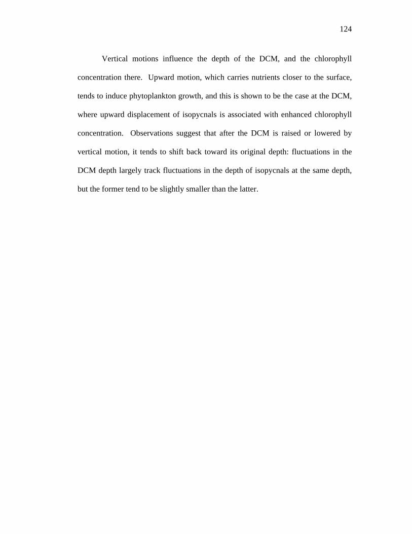
124

Vertical motions influence the depth of the DCM, and the chlorophyll

concentration there. Upward motion, which carries nutrients closer to the surface,

tends to induce phytoplankton growth, and this is shown to be the case at the DCM,

where upward displacement of isopycnals is associated with enhanced chlorophyll

concentration. Observations suggest that after the DCM is raised or lowered by

vertical motion, it tends to shift back toward its original depth: fluctuations in the

DCM depth largely track fluctuations in the depth of isopycnals at the same depth,

but the former tend to be slightly smaller than the latter.

125

Longitude

Latit

ude

−123 −122 −121 −120 −119 −118 −117 −11629

30

31

32

33

Apr−Jun 2005Dec 2005−Feb 2006Mar−May 2006CalCOFI Line 93 station

Dep

th /

Ele

vatio

n (m

)

−5000

−4000

−3000

−2000

−1000

0

1000

Figure 4.1. Tracks from the three glider deployments, and CalCOFI Line 93 station locations. The first deployment (red) ended after completion of half of the return transect. The track from the second deployment is plotted in blue, and that from the third in green.

126

0

20

40

60

80

Pre

ssur

e (d

bar)

0

20

40

60

80

Longitude−119 −118.8 −118.6 −118.4 −118.2 −118

0

20

40

60

80

Chl

orop

hyll

(mg/

m3 )

0

0.2

0.4

0.6

0.8

1

1.2

1.4

1.6

1.8

2

Figure 4.2. A week of chlorophyll fluorescence data from the outward leg of the spring 2006 glider deployment. Top panel: raw fluorescence measurments converted to chlorophyll concentration. Middle panel: the same section after correction for nonphotochemical quenching. Bottom panel: the correction. The black line at the top shows relative light intensity, based on the position of the sun. Black dots indicate the location of each dive.

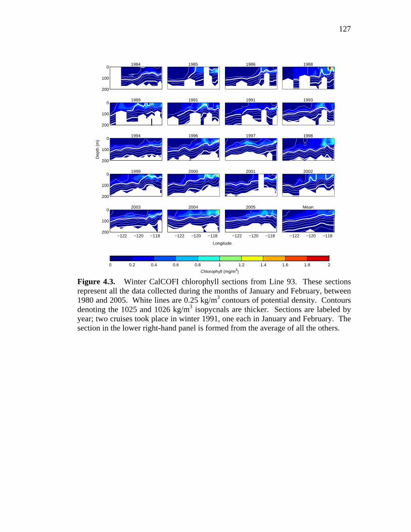
127

19840

100

200

1985 1986 1988

19890

100

200

1991 1991 1993D

epth

(m

)

19940

100

200

1996 1997 1998

19990

100

200

2000 2001 2002

2003

−122 −120 −118

0

100

200

Longitude

2004

−122 −120 −118

2005

−122 −120 −118

Chlorophyll (mg/m3)

0 0.2 0.4 0.6 0.8 1 1.2 1.4 1.6 1.8 2

Mean

−122 −120 −118

Figure 4.3. Winter CalCOFI chlorophyll sections from Line 93. These sections represent all the data collected during the months of January and February, between 1980 and 2005. White lines are 0.25 kg/m3 contours of potential density. Contours denoting the 1025 and 1026 kg/m3 isopycnals are thicker. Sections are labeled by year; two cruises took place in winter 1991, one each in January and February. The section in the lower right-hand panel is formed from the average of all the others.

128

19810

100

200

1984 1985 1986

19870

100

200

1988 1989 1990D

epth

(m

)

19920

100

200

1993 1995 1996

19970

100

200

1998 1999 2000

2001

−122 −120 −118

0

100

200

Longitude

2003

−122 −120 −118

2005

−122 −120 −118

Chlorophyll (mg/m3)

0 0.2 0.4 0.6 0.8 1 1.2 1.4 1.6 1.8 2

Mean

−122 −120 −118

Figure 4.4. As in Fig. 4.3, but for CalCOFI observations collected along Line 93 during the spring (April and May).

129

Longitude (deg)

Pre

ssur

e (d

bar)

6/14

/05

5/19

/05 −20

0

20

Cur

rent

(cm

/s)

−123 −122 −121 −120 −119 −118

0

40

80

120

160

200

Pre

ssur

e (d

bar)

4/21

/05

5/19

/05

0

40

80

−20

0

20

Cur

rent

(cm

/s)120

160

200−123 −122 −121 −120 −119 −118

0 0.2 0.4 0.6 0.8 1 1.2 1.4 1.6 1.8 2

Chlorophyll (mg/m3)

Figure 4.5. Chlorophyll sections (upper 200 meters only) from the first glider deployment. Black lines are contours of potential density, spaced every 0.2 kg/m3, with the 1024, 1025, and 1026-kg/m3 isopycnals denoted by thicker lines. These sections may be compared with the springtime CalCOFI observations (Fig. 4.3). The glider began near San Diego and proceeded to the end of CalCOFI Line 93 (right to left in the upper panel of the figure), and then reversed course, repeating the transect (left to right in the lower panel). The mission ended on June 19 near –120° longitude, due to a mechanical failure, but the last 5 days of fluorescence data are not shown, as severe biofouling (already obvious in the portion of the return transect shown in the lower panel above) obscured all useful information about chlorophyll during that time. The location of each dive is denoted by a black hash mark at the top of each panel, and the ends of each section are labeled by date. The red stick plots near the bottom of each panel show inferred current velocity (see text). In these plots, the horizontal and vertical directions represent along- and across-track velocity components, respectively. An upward pointing stick indicates a current flowing into the page, a downward stick one flowing out of the page.

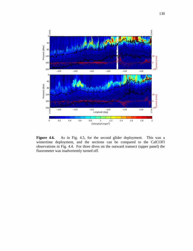
130

Longitude (deg)

Pre

ssur

e (d

bar)

2/7/

06

1/14

/06 −20

0

20

Cur

rent

(cm

/s)

−123 −122 −121 −120 −119 −118

0

40

80

120

160

200

Pre

ssur

e (d

bar)

12/9

/05

1/14

/06

0

40

80

−20

0

20

Cur

rent

(cm

/s)120

160

200−123 −122 −121 −120 −119 −118

0 0.2 0.4 0.6 0.8 1 1.2 1.4 1.6 1.8 2

Chlorophyll (mg/m3)

Figure 4.6. As in Fig. 4.5, for the second glider deployment. This was a wintertime deployment, and the sections can be compared to the CalCOFI observations in Fig. 4.4. For three dives on the outward transect (upper panel) the fluorometer was inadvertently turned off.

131

Longitude (deg)

Pre

ssur

e (d

bar)

5/18

/06

4/19

/06 −20

0

20

Cur

rent

(cm

/s)

−123 −122 −121 −120 −119 −118

0

40

80

120

160

200

Pre

ssur

e (d

bar)

3/15

/06

4/19

/06

0

40

80

−20

0

20

Cur

rent

(cm

/s)120

160

200−123 −122 −121 −120 −119 −118

0 0.2 0.4 0.6 0.8 1 1.2 1.4 1.6 1.8 2

Chlorophyll (mg/m3)

Figure 4.7. As in Fig. 4.5, for the third glider deployment. Compare to Fig. 4.3.

132

19840

200

400

1985 1986 1988

19890

200

400

1991 1991 1993D

epth

(m

)

19940

200

400

1996 1997 1998

19990

200

400

2000 2001 2002

2003

−122 −120 −118

0

200

400

Longitude

2004

−122 −120 −118

2005

−122 −120 −118

Salinity (psu)33 33.2 33.4 33.6 33.8 34 34.2

Mean

−122 −120 −118

Figure 4.8. As in Fig. 4.3, but for winter CalCOFI salinity sections, rather than chlorophyll. Instead of only 200, the upper 500 meters are shown, and the black lines are contours of potential density spaced every 0.5 kg/m3, with heavier lines for 1025 and 1026 kg/m3.

133

19810

200

400

1984 1985 1986

19870

200

400

1988 1989 1990D

epth

(m

)

19920

200

400

1993 1995 1996

19970

200

400

1998 1999 2000

2001

−122 −120 −118

0

200

400

Longitude

2003

−122 −120 −118

2005

−122 −120 −118

Salinity (psu)33 33.2 33.4 33.6 33.8 34 34.2

Mean

−122 −120 −118

Figure 4.9. As in Fig. 4.8, for springtime CalCOFI sections (April and May).

134

Longitude (deg)

Pre

ssur

e (d

bar)

6/19

/05

5/19

/05 −20

0

20

Cur

rent

(cm

/s)

−123 −122 −121 −120 −119 −118

0

100

200

300

400

500

Pre

ssur

e (d

bar)

4/21

/05

5/19

/05

−20

0

20

Cur

rent

(cm

/s)

−123 −122 −121 −120 −119 −118

0

100

200

300

400

500

Salinity (PSU)33 33.2 33.4 33.6 33.8 34 34.2

Figure 4.10. Salinity sections from the first glider deployment. Layout is identical to Fig. 4.5, except that the full 500-meter section is shown, rather than only the upper 200 meters. This was a springtime deployment, and the sections may be compared to Fig. 4.9.

135

Longitude (deg)

Pre

ssur

e (d

bar)

2/7/

06

1/14

/06 −20

0

20

Cur

rent

(cm

/s)

−123 −122 −121 −120 −119 −118

0

100

200

300

400

500

Pre

ssur

e (d

bar)

12/9

/05

1/14

/06

−20

0

20

Cur

rent

(cm

/s)

−123 −122 −121 −120 −119 −118

0

100

200

300

400

500

Salinity (PSU)33 33.2 33.4 33.6 33.8 34 34.2

Figure 4.11. As in Fig. 4.10 for the second glider deployment. Compare to Fig. 4.8 (winter CalCOFI observations).

136

Longitude (deg)

Pre

ssur

e (d

bar)

5/18

/06

4/19

/06 −20

0

20

Cur

rent

(cm

/s)

−123 −122 −121 −120 −119 −118

0

100

200

300

400

500

Pre

ssur

e (d

bar)

3/15

/06

4/19

/06

−20

0

20

Cur

rent

(cm

/s)

−123 −122 −121 −120 −119 −118

0

100

200

300

400

500

Salinity (PSU)33 33.2 33.4 33.6 33.8 34 34.2

Figure 4.12. As in Fig. 4.10 for the third glider deployment. Compare to Fig. 4.9.

137

Longitude

Dep

th (

m)

−120.2 −120 −119.8 −119.6 −119.4 −119.2 −119

0

50

100

150

200

250

300

350

400

Log chlorophyll (mg/m3)

−2.5 −2 −1.5 −1 −0.5 0 0.5

Figure 4.13. Salinity contours plotted over chlorophyll fluorescence for a density-compensated salinity intrusion from the return transect of the second glider deployment. Salinity contour spacing is 0.1 PSU, with a thicker line for the 34 PSU contour. Chlorophyll is displayed on a logarithmic scale to emphasize the small chlorophyll concentrations below the DCM layer.

138

1024 1024.2 1024.4 1024.6 1024.8 1025 1025.2 1025.4 1025.6−0.8

−0.6

−0.4

−0.2

0

0.2

0.4

0.6

0.8

Density (kg/m3)

Den

sity

Ano

mal

y (k

g/m

3 )

Log

Chl

orop

hyll

(mg/

m3 )

−0.3

−0.2

−0.1

0

0.1

0.2

0.3

0.4

0.5

0.6

0.7

Figure 4.14. For each of the dives in all three glider deployments, density anomaly at the DCM is plotted versus potential density there as a point whose color is scaled by the chlorophyll concentration at the DCM. The color scale is logarithmic to de-emphasize the few profiles with very high chlorophyll concentrations. Density anomaly is defined as the difference between the measured density at the location of the DCM and the density expected at that location and depth on the basis of historical CalCOFI data. When isopycnals are displaced upward, density anomaly is positive; when downward, negative. The correlation between density and density anomaly indicates that when the DCM is displaced upward (downward) by vertical motion, it moves deeper (shallower), into denser (lighter) water. The larger chlorophyll concentrations toward the top of the plot indicate that positive density anomalies (isopycnals displaced upward) are associated with higher chlorophyll concentrations.

References

Abraham, E.R., 1998. The generation of plankton patchiness by turbulent stirring. Nature 391, 577-580. Batchelor, G.K., 1952. The effect of homogenous turbulence on material lines and surfaces. Proceedings of the Royal Society of London, A, 213, 349-366. Bishop, J.K.B., 1999. Transmissometer measurement of POC. Deep-Sea Research I 46, 353–369. Bricaud, A., Morel, A., Prieur, L., 1983. Optical efficiency factors of some phytoplankters. Limnology and Oceanography 28, 816–832. Briscoe, M.G., 1977. Gaussianity of internal waves. Journal of Geophysical Research, 82, C15, 2117-2126. Chelton, D.B., Bernal, P.A., McGowan, J.A., 1982. Large-scale interanual physical and biological interaction in the California Current. Journal of Marine Research, 40, 4, 1095-1125. Childress, S., Gilbert, A.D., 1995. Stretch, Twist, Fold: The Fast Dynamo. Springer-Verlag Lecture Notes in Physics: Monographs, 37. Criminale, W.O., Winter, D.F., 1974. The stability of steady-state depth distributions of marine phytoplankton. The American Naturalist 108 (963), 679–687. Cullen, J.J., 1982. The deep chlorophyll maximum: comparing vertical profiles of chlorophyll a. Canadian Journal of Fisheries and Aquatic Sciences 39, 791–803. Cullen, J.J., Lewis, M.R., 1988. The kinetics of algal photoadaptation in the context of vertical mixing. Journal of Plankton Research 10 (5), 1039-1063. Cushing, D.H., 1961. Patchiness. ICES, Symposium on Zooplankton Production, 14, 15. Daubechies, I., 1992. Ten Lectures on Wavelets. CBMS-NSF Regional Conference Series in Applied Mathematics (Society for Industrial and Applied Mathematics, Philadelphia, 1992). Denman, K.L., 1976. Covariability of chlorophyll and temperature in the sea. Deep-Sea Research 23, 539-550.

139

140

Denman, K.L., Okubo, A., Platt, T., 1977. The chlorophyll fluctuation spectrum in the sea. Limnology and Oceanography 22, 1033–1038. Denman, K.L., Platt, T., 1976. The variance spectrum of phytoplankton in a turbulent ocean. Journal of Marine Research 34, 593-601. Eckart, C., 1948. An analysis of the stirring and mixing processes in incompressible fluids. Journal of Marine Research, 7, 265-275. Edwards, C.A., Powell, T.A., Batchelder, H.P., 2000. The stability of an NPZ model subject to realistic levels of vertical mixing. Journal of Marine Research 58, 37–60. Falkowski, P., Kiefer, D.A., 1985. Chlorophyll a fluorescence in phytoplankton: relationship to photosynthesis and biomass. Journal of Plankton Research 7 (5), 715-731. Fasham, M.J.R., Ducklow, H.W., McKelvie, S.M., 1990. A nitrogen-based model of plankton dynamics in the oceanic mixed layer. Journal of Marine Research 48, 591–639. Fennel, K., Boss, E., 2003. Subsurface maxima of phytoplankton and chlorophyll: steady state solutions from a simple model. Limnology and Oceanography 48 (4), 1521–1534. Ferrari, R., Rudnick, D.L., 2000. Thermohaline variability in the upper ocean. Journal of Geophysical Research, 105, 16,857-16,883. Franks, P.J.S., Wroblewski, J.S., Flierl, G.R., 1986. Behavior of a simple plankton model with food-level acclimation by herbivores. Marine Biology 91, 121–129. Hardy, A.C., 1936. Observations on the uneven distribution of oceanic plankton. Discovery Reports 11, 511-538. Iselin, C.O., 1939. The influence of vertical and lateral turbulence on the characteristics of the waters at mid-depths. Trans. of the Amer. Geophys. Union, 1939, 414-417. Jamart, B.M., Winter, D.F., Banse, K., Anderson, G.C., Lam, R.K., 1977. A theoretical study of phytoplankton growth and nutrient distribution in the Pacific Ocean off the northwestern US coast. Deep-Sea Research 24, 753–773. Jenkins, W.J., Goldman, J.C., 1985. Seasonal oxygen cycling and primary production in the Sargasso Sea. Journal of Marine Research 43, 465–491.

141

Kiefer, D.A., 1973. Fluorescence properties of natural phytoplankton populations. Marine Biology, 22, 3, 263-269. Kitchen, J.C., Zaneveld, J.R.V., 1990. On the noncorrelation of the vertical structure of light scattering and chlorophyll a in Case I waters. Journal of Geophysical Research 95 (C11), 20,237–20,246. Krause, G.H., Weis, E., 1991. Chlorophyll fluorescence and photosynthesis: The basics. Annual Review of Plant Physiology and Plant Molecular Biology, 42, 313-349. Ledwell, J.R., Watson, A.J., Law, C.S., 1993. Evidence for slow mixing across the pycnocline from an open-ocean tracer-release experiment, Nature, 364, 701-703. Ledwell, J.R., Watson, A.J., Law, C.S., 1998. Mixing of a Tracer in the Pycnocline, Journal of Geophysical Research, 103(C10), 21499-21530. Lima, I.D., Olson, D.B., Doney, S.C., 2002. Intrinsic dynamics and stability properties of size-structured pelagic ecosystem models. Journal of Plankton Research 24 (6), 533–556. Lorenzen, C.J., 1966. A method for the continuous measurement of in vivo chlorophyll concentration. Deep-Sea Research 13, 223–227. MacIntyre, H.L., Kana, T.M., Anning, T., Geider, R.J., 2002. Photoacclimation of photosynthesis irradiance response curves and photosynthetic pigments in microalgae and cyanobacteria. Journal of Phycology 38, 17-38. Mann, K.H., Lazier, J.R. N., 1996. Dynamics of Marine Ecosystems. Blackwell Science, Oxford. Martin, A.P., 2003. Phytoplankton patchiness: the role of lateral stirring and mixing. Progress in Oceanography 57, 125-174. Olson, R.J., 1981. Differential photoinhibition of marine nitrifying bacteria: a possible mechanism for the formation of the primary nitrite maximum. Journal of Marine Research 39 (2), 227–238. Pak, H., Kiefer, D.A., Kitchen, J.C., 1988. Meridional variations in the concentration of chlorophyll and microparticles in the North Pacific Ocean. Deep-Sea Research 35, 7, 1151-1171. Pierrehumbert, R. T., 1994. Tracer Microstructure in the Large-eddy Dominated Regime. Chaos, Solitons & Fractals 4, 6, 1091-1110.

142

Redfield, A.C., Ketchum, B.H., Richards, F.A., 1982. The influence of organisms on the composition of seawater. In: Hill, M. N. (Ed.), The Sea, Vol. 2. Wiley, New York, pp. 26–77. Riley, G.A., Stommel, H., Bumpus, D.F., 1949. Quantitative ecology of the plankton of the western North Atlantic. Bulletin of the Bingham Oceanographic Collection 12 (3), 1–169. Roemmich, D., McGowan, J., 1995. Climatic Warming and the Decline of Zooplankton in the California Current. Science 267, 5202, 1324-1326. Rudnick, D.L., Ferrari, R., 1999. Compensation of Horizontal Temperature and Salinity Gradients in the Ocean Mixed Layer. Science, 283, 526-529. Rudnick, D.L., Luyten, J.R., 1996. Intensive surveys of the Azores Front 1. Tracers and dynamics. Journal of Geophysical Research, 101, C1, 923-939. Sherman, J., Davis, R.E., Owens, W.B., Valdes, J., 2001. The autonomous underwater glider “Spray”. IEEE Journal of Oceanic Engineering, 26, 4, 437-446. Shulenberger, E., Reid, J.L., 1981. The Pacific shallow oxygen maximum, deep chlorophyll maximum, and primary productivity, reconsidered. Deep-Sea Research, 28A, 9, 901-919. Smethie Jr., W.M., Fine, R.A., 2001. Rates of North Atlantic Deep Water formation calculated from chlorofluorocarbon inventories. Deep-Sea Research I, 48, 189-215. Steele, J.H., 1974. The Structure of Marine Ecosystems. Harvard University Press, Cambridge. Steele, J.H., Yentsch, C.S., 1960. The vertical distribution of chlorophyll. Journal of the Marine Biological Association of the United Kingdom 39, 217–226. Varela, R.A., Cruzado, A., Tintoré, J., Ladona, E.G., 1992. Modelling the deep-chlorophyll maximum: a coupled physical–biological approach. Journal of Marine Research 50, 441–463. Varela, R.A., Cruzado, A., Tintoré, J., 1994. A simulation analysis of various biological and physical factors influencing the deep-chlorophyll maximum structure in oligotrophic areas. Journal of Marine Systems 5, 143–157. Venrick, E.L., 1993. Phytoplankton seasonality in the central North Pacific: the endless summer reconsidered. Limnology and Oceanography 38, 1135–1149.

143

Venrick, E.L., McGowan, J.A., Mantyla, A.W., 1973. Deep maxima of photosynthetic chlorophyll in the Pacific Ocean. Fishery Bulletin (US) 71, 41–52. Warhaft, Z., 2000. Passive Scalars in Turbulent Flows. Annual Reviews of Fluid Mechanics 32, 203-240. Winn, C.D., Campbell, L., Christian, J.R., Letelier, R.M., Hebel, D.V., Dore, J.E., Fujieki, L., Karl, D.M., 1995. Seasonal variability in the phytoplankton community of the North Pacific Subtropical Gyre. Global Biogeochemical Cycles 9 (4), 605–620. Yentsch, C.S., Yentsch, C.M., 1979. Fluorescence spectral signatures: the characterization of phytoplankton populations by the use of excitation and emission spectra. Journal of Marine Research 37, 471–483. Young, W.R., Roberts, A.J., Stuhne, G., 2001. Reproductive pair correlations and the clustering of organisms. Nature 412, 328-331.