university of cambridge engineering part iib module...

University of Cambridge

Engineering Part IIB

Module 4F12: Computer Vision and

Robotics

Handout 1: Introduction

Roberto CipollaOctober 2012

Introduction 1

What is computer vision?

Vision is about discovering from images what ispresent in the scene and where it is. It is our mostpowerful sense.

In computer vision a camera (or several cameras)is linked to a computer. The computer automati-cally interprets images of a real scene to obtain use-ful information (3R’s: registration, recognition andreconstruction) and then acts on that information(e.g. for navigation, manipulation or recognition).

images → representation

perception → actions

It is not :

Image processing: image enhancement, image restora-tion, image compression. Take an image andprocess it to produce a new image which is, insome way, more desirable.

Pattern recognition: classifies patterns into oneof a finite set of prototypes.

2 Engineering Part IIB: 4F12 Computer Vision

Why study computer vision?

1. Intellectual curiosity — how do we see?

2. Replicate human vision to allow a machine to see— many industrial applications.

Applications

• Automation of industrial processes

– Object recognition.

– Visual inspection.

– Robot hand-eye coordination

– Robot navigation.

Introduction 3

Applications

• Space and Military

– Remote sensing

– Surveillance - target detection and tracking

– UAV localisation

• Surveillance and tracking (traffic, aircraft, watch-ing humans and motion capture)

• Human-computer interaction

– Face detection and recognition.

– Gesture-based HCI (e.g. new interfaces forgames consoles)

– Image search and retrieval from video and im-age databases

– Mobile-phone applications - target/object recog-nition, mosaicing

– Augmented reality

• 3D modelling, measurement and visualisation

– 3D model building from image sequences

– Photogrammetry.

• Automotive applications and autonomous vehi-cles


How to study vision? The eye

Let’s start with the human visual system.

• Retina measures about 1000 mm2 and containsabout 108 sampling elements (rods) (and about106 cones for sampling colour).

• The eye’s spatial resolution is about 0.01 over a150 field of view (not evenly spaced, there is afovea and a peripheral region).

• Intensity resolution is about 11 bits/element, spec-tral resolution is about 2 bits/element (400–700nm).

• Temporal resolution is about 100 ms (10 Hz).

• Two eyes (each about 2cm in diameter), sepa-rated by about 6cm.

Introduction 5

• A large chunk of our brain is dedicated to pro-cessing the signals from our eyes - a data rate ofabout 3 GBytes/s!


Why not copy the biology?

• There is no point copying the eye and brain —human vision involves 60 billion neurons!

• Evolution took its course under a set of con-straints that are very different from today’s tech-nological barriers.

• The computers we have available cannot performlike the human brain.

• We need to understand the underlying principlesrather than the particular implementation.

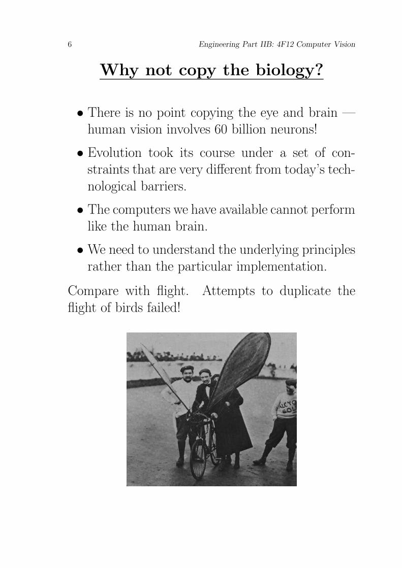
Compare with flight. Attempts to duplicate theflight of birds failed!

Introduction 7

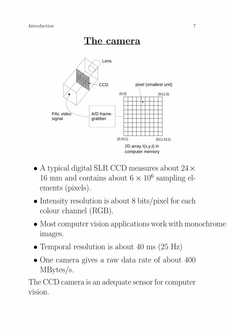
The camera

grabberA/D frame-PAL video

signal

Lens

pixel (smallest unit)

(0,0) (511,0)

(511,511)(0,511)

2D array I(x,y,t) incomputer memory

CCD

• A typical digital SLR CCD measures about 24×16 mm and contains about 6 × 106 sampling el-ements (pixels).

• Intensity resolution is about 8 bits/pixel for eachcolour channel (RGB).

• Most computer vision applications work with monochromeimages.

• Temporal resolution is about 40 ms (25 Hz)

• One camera gives a raw data rate of about 400MBytes/s.

The CCD camera is an adequate sensor for computervision.


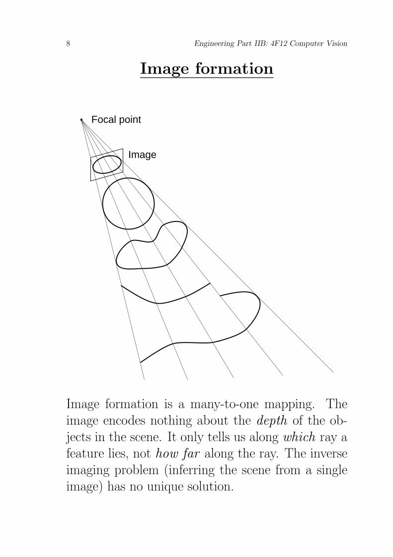
Image formation

Focal point

Image

Image formation is a many-to-one mapping. Theimage encodes nothing about the depth of the ob-jects in the scene. It only tells us along which ray afeature lies, not how far along the ray. The inverseimaging problem (inferring the scene from a singleimage) has no unique solution.

Introduction 9

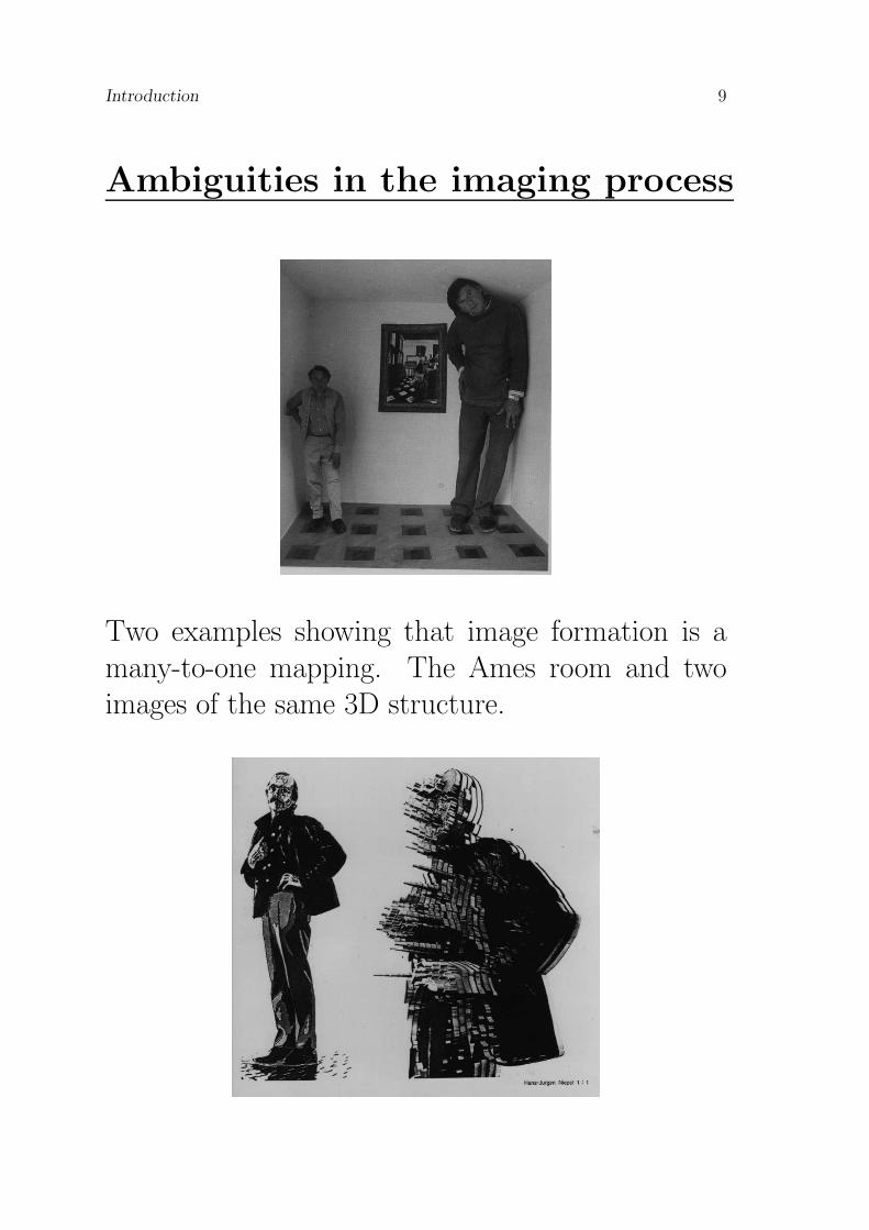
Ambiguities in the imaging process

Two examples showing that image formation is amany-to-one mapping. The Ames room and twoimages of the same 3D structure.


Vision as information processing

David Marr, one of the pioneers of computer vision,said:“ One cannot understand what seeing is and how

it works unless one understands the underlying

information processing tasks being solved.”

From an information processing point of view, visioninvolves a huge amount of data reduction:

images → generic salient features

10 MBytes/s 10 KBytes/s

(mono CCD)

salient features → representations and actions

10 KBytes/s 1–10 bits/s

Vision is also about resolving the ambiguities inher-ent in the imaging process, by drawing on a set ofconstraints (AI). But where do the constraints comefrom? We have two options:

1. Use more than one image of the scene.

2. Make assumptions about the world in the scene.

Introduction 11

Feature extraction

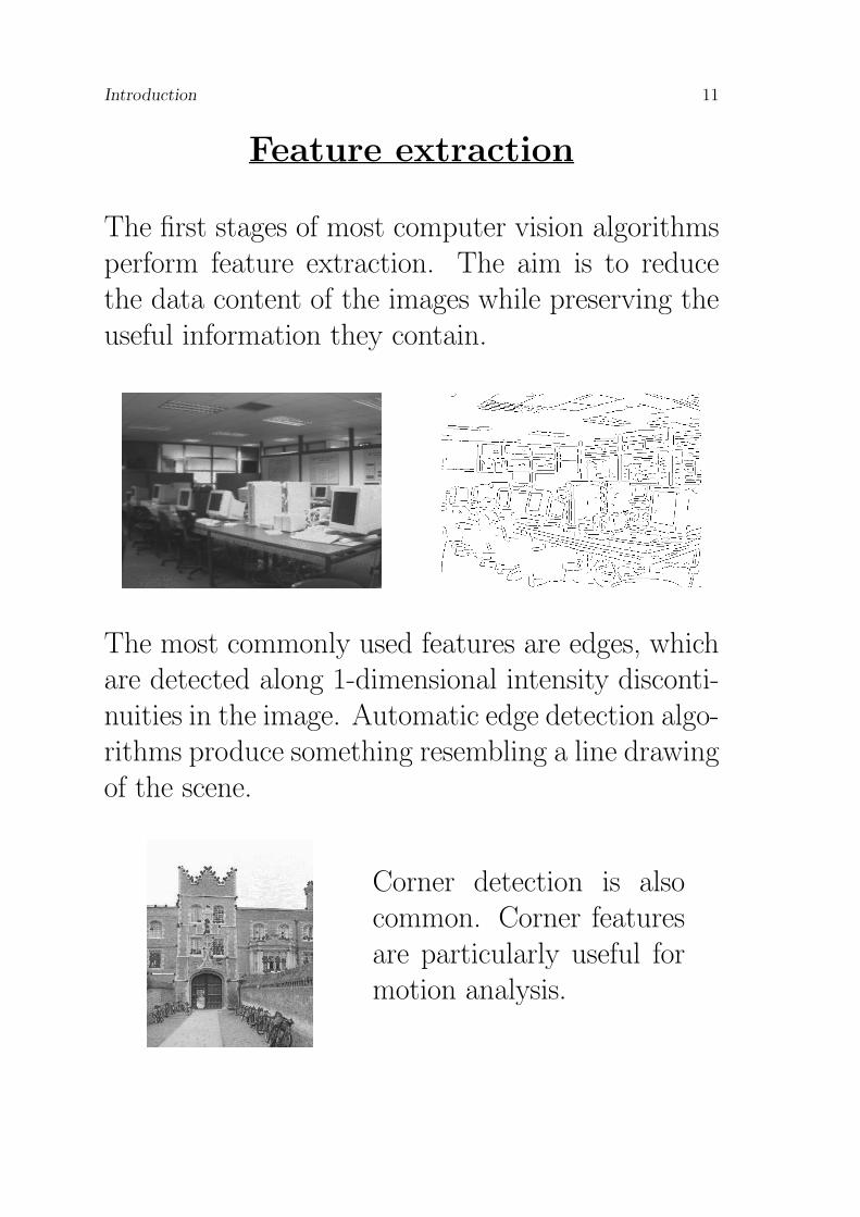
The first stages of most computer vision algorithmsperform feature extraction. The aim is to reducethe data content of the images while preserving theuseful information they contain.

The most commonly used features are edges, whichare detected along 1-dimensional intensity disconti-nuities in the image. Automatic edge detection algo-rithms produce something resembling a line drawingof the scene.

Corner detection is alsocommon. Corner featuresare particularly useful formotion analysis.


Camera models

Before we attempt to interpret the image (or thefeatures extracted from the image), we have to un-derstand how the image was formed. In other words,we have to develop a camera model.

Camera-centeredcoordinates

Worldcoordinates

Opticalaxis

Imageplane

Xc

Opticalcentre

Zc

X

Y

c

c

X

Y

Z

X

p

x

f

Camera models must account for the position ofthe camera, perspective projection and CCD imag-ing. These geometric transformations have beenwell-understood since the C14th. They are best de-scribed within the framework of projective ge-

ometry.

Introduction 13

Camera models

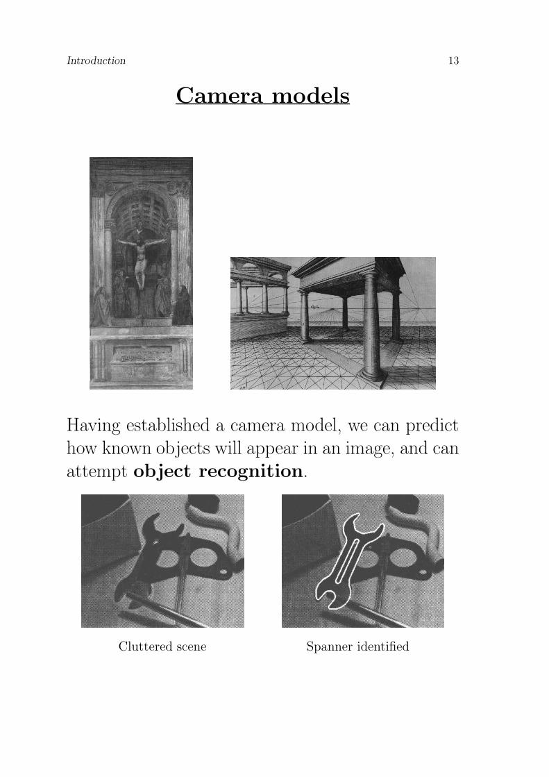
Having established a camera model, we can predicthow known objects will appear in an image, and canattempt object recognition.

Cluttered scene Spanner identified


Shape from texture

Texture provides a very strong cue for inferring sur-face orientation in a single image. It is necessary toassume homogeneous or isotropic texture. Then,it is possible to infer the orientation of surfaces byanalysing how the texture statistics vary over theimage.

Here we perceive a verticalwall slanted away from thecamera.

And here we perceive ahorizontal surface belowthe camera.

Introduction 15

Stereo vision

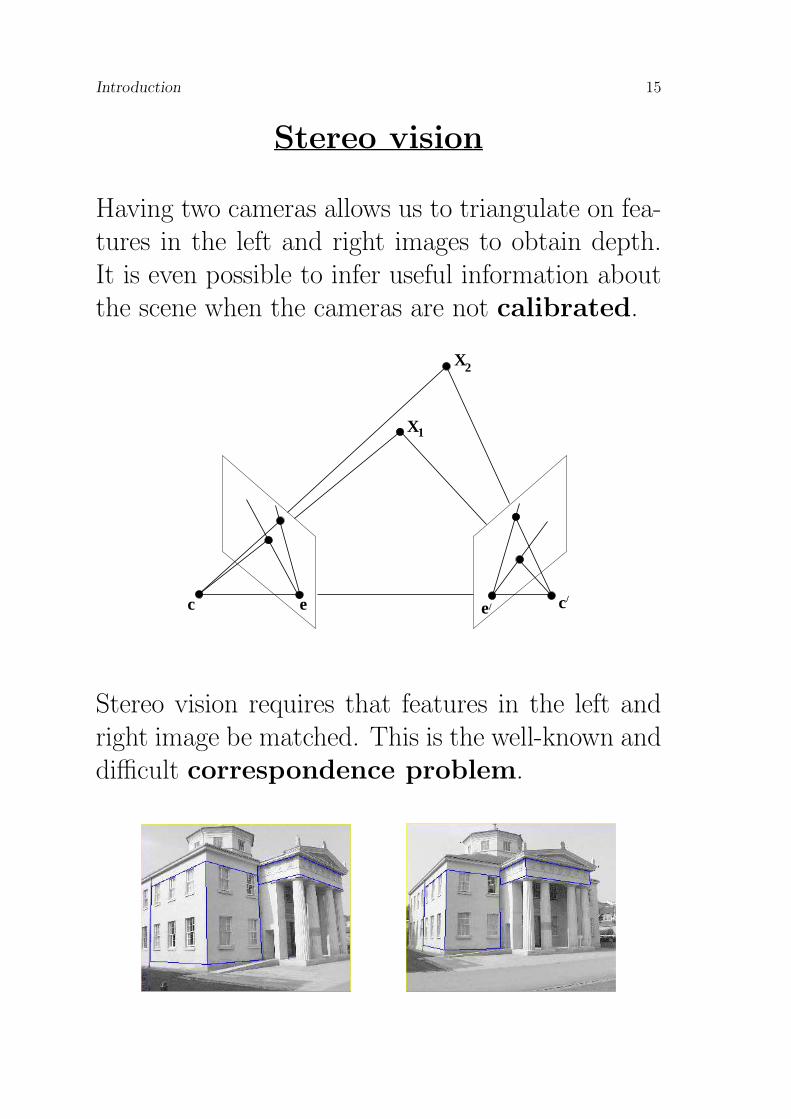
Having two cameras allows us to triangulate on fea-tures in the left and right images to obtain depth.It is even possible to infer useful information aboutthe scene when the cameras are not calibrated.

e e

X

/

2

1

cc

X

/

Stereo vision requires that features in the left andright image be matched. This is the well-known anddifficult correspondence problem.


Structure from motion

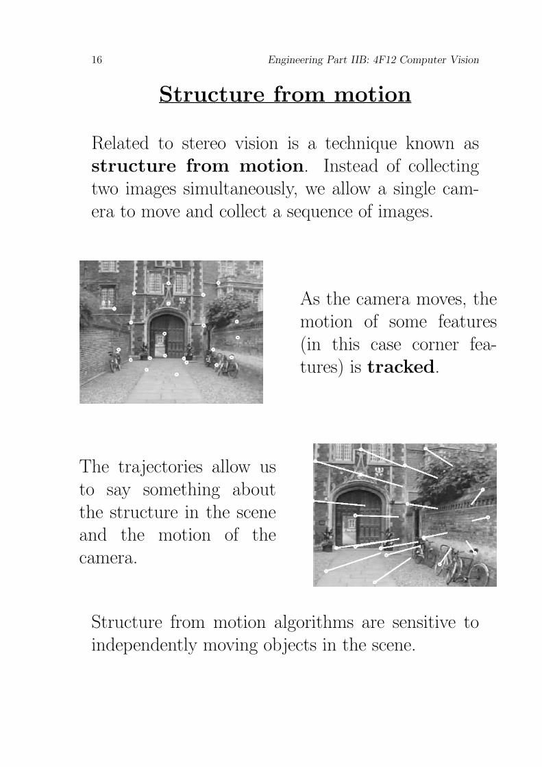
Related to stereo vision is a technique known asstructure from motion. Instead of collectingtwo images simultaneously, we allow a single cam-era to move and collect a sequence of images.

As the camera moves, themotion of some features(in this case corner fea-tures) is tracked.

The trajectories allow usto say something aboutthe structure in the sceneand the motion of thecamera.

Structure from motion algorithms are sensitive toindependently moving objects in the scene.

Introduction 17

Shape from line drawings

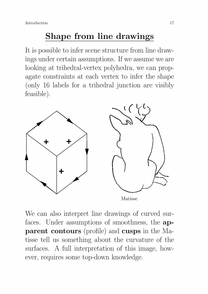
It is possible to infer scene structure from line draw-ings under certain assumptions. If we assume we arelooking at trihedral-vertex polyhedra, we can prop-agate constraints at each vertex to infer the shape(only 16 labels for a trihedral junction are visiblyfeasible).

+

+

+

Matisse

We can also interpret line drawings of curved sur-faces. Under assumptions of smoothness, the ap-

parent contours (profile) and cusps in the Ma-tisse tell us something about the curvature of thesurfaces. A full interpretation of this image, how-ever, requires some top-down knowledge.


Shape from contour

A curved surface is bounded by its apparent con-

tours in an image. Each contour defines a set oftangent planes from the camera to the surface.

As the camera moves, the contour generators “slip”over the curved surface. By analysing the defor-mation of the apparent contours in the image, it ispossible to reconstruct the 3D shape of the curvedsurface.

c

c

1

2

Introduction 19

Shape from shading

It is possible to infer the structure in a scene fromthe shading observed in the image.

Assumptions we make in-clude a Lambertian lightsource, isotropic surfacereflectance, and a top-litscene.

The self shadows ofan object give particularlyrich information.

Peter Paul Rubens

Samson and Delilah (detail)


Human visual capabilities

Our visual system allows us to successfully interpretimages under a wide range of conditions. It is notsurprising that we can cope with normal stereo vi-sion: we have two eyes to use for triangulation, anda number of other cues (motion, shading etc.) tohelp us.

More surprising is our ability to interpret a widerange of images with limited cues.

Introduction 21

Geometrical framework

The first part of the course will focus on genericcomputer vision techniques which make minimal as-sumptions about the outside world. This meanswe’ll be concentrating on the theory of perspective,stereo vision and structure from motion.

We typically use a geometric framework:

1. Reduce the information content of the images toa manageable size by extracting salient features,typically edges or blobs . (These features aregeneric and substantially invariant to a varietyof lighting conditions.)

2. Model the imaging process, usually as a per-spective projection and express using projectivetransformations.

3. Invert the transformation using as many imagesand constraints as necessary to extract 3D struc-ture and motion.


Statistical framework

Geometry alone is only a part of the solution. Inthe second part of the course we will introduce tech-niques which learn from the visual world. They arepart of a statistical framework to understanding vi-sion and for building systems which:

1. Have the ability to test hypotheses

2. Deal with the ambiguity of the visual world

3. Are able to fuse information

4. Have the ability to learn

Many of these requirements can be addressed byreasoning with probabilities and are the subject ofother advanced courses on Statistical Pattern Recog-nition and Machine Learning.

Introduction 23

Syllabus

1. Introduction

• Computer vision: what is it, why study it and how?• Vision as an information processing task• A geometrical framework for vision• 3D interpretation of 2D images

2. Image structure

• Image intensities and structure: edges, corners and blobs• Edge detection, the aperture problem, corner detection, blob de-

tection• Texture.• Feature descriptors and matching of features.

3. Projection

• Orthographic projection• Planar perspective projection, vanishing points and lines.• Projection matrix, homogeneous coordinates• Camera calibration, recovery of world position• Weak perspective, the affine camera

4. Stereo vision and Structure from Motion

• Epipolar geometry and the essential matrix• Recovery of depth• Uncalibrated cameras and the fundamental matrix• The correspondence problem• Structure from motionm• 3D shape with multiple view stereo.

5. Object detection and tracking

• Basic target tracking.• Object detection using support vector machines and boosting• Chamfer matching and template trees

Course book: V. S. Nalwa. A Guided Tour Of Computer Vision,Addison-Wesley, 1993 (CUED shelf mark: NO 219).


Further reading

Students looking for a deeper understanding of computer vision mightwish to consult the following publications, many of which are available

in the CUED library.

Journals

International Journal of Computer VisionIEEE Transactions on Pattern Analysis and Machine IntelligenceImage and Vision Computing

Computer Vision, Graphics and Image Processing

Conference proceedings

International Conference on Computer VisionEuropean Conference on Computer Vision

Computer Vision and Pattern Recognition ConferenceBritish Machine Vision Conference

Books

R. Cipolla and P. Giblin Visual Motion of Curves and Surfaces. CUP,

1999.

D.A. Forsyth and J. Ponce. Computer Vision - A Modern Approach.

Prentice Hall 2003.

R. Hartley and A. Zisserman. Multiple View Geometry.CUP 2000.

J. J. Koenderink. Solid shape. MIT Press, 1990.

D. Marr. Vision: a computational investigation into the human rep-

resentation and processing of visual information. Freeman, 1982.

S.J.D. Prince Computer Vision: Models, Learning and Inference. CUP,2012.

R. Szeliski. Computer Vision: algorithms and applications. Springer,

2011.

B. A. Wandell. Foundations of vision. Sinauer Associates, 1995.

See also the bibliographies at the end of each handout.

Introduction 25

Mathematical Preliminaries

Linear least squares

Consider a set of m linear equations

Ax = b

where x is an n-element vector of unknowns, b isan m-element vector and A is an m × n matrix ofcoefficients. If m > n then the set of equations isover-constrained and it is generally not possible tofind a precise solution x.

The equations can, however, be solved in a least

squares sense. That is, we can find a vector x

which minimizesm∑

i=1r2i

whereAx = b + r

r is the vector of residuals.

The least squares solution is found with the aid ofthe pseudo-inverse:

A† =(

ATA)−1

AT

The least squares solution is then given by x = A† b.


Mathematical Preliminaries

Eigenvectors and eigenvalues

Often the equations can be written as a set of m

linear equations

Ax = 0

where x is an n-element vector of unknowns and Ais an m × n matrix of coefficients.

A non-trivial solution for x (up to an arbitrary mag-nitute) can be found if m > n. The solution is cho-sen to minimize the residuals given by |Ax| subjectto |x| = 1.

By considering Rayleigh’s Quotient:

λ1 ≤xTATAx

xTx≤ λn

it is easy to show that the solution is the eigenvectorcorresponding to the smallest eigenvalue of the n×n

symmetric matrix ATA.

Introduction 27

Notation

Metric coordinates

Camera-centeredcoordinates

Worldcoordinates

Opticalaxis

Imageplane

Xc

Opticalcentre

Zc

X

Y

c

c

X

Y

Z

X

p

x

f

World coordinates

X = (X, Y, Z) Point in 3D space

Xp = (X, Y ) Point on 2D plane

Xl = (X) Point on 1D line

Camera-centered coordinates

Xc = (Xc, Yc, Zc) Point in 3D space

p = (x, y, f) Ray to point on image plane

x = (x, y) Image plane coordinates

Pixel coordinates

w = (u, v) Pixel coordinates


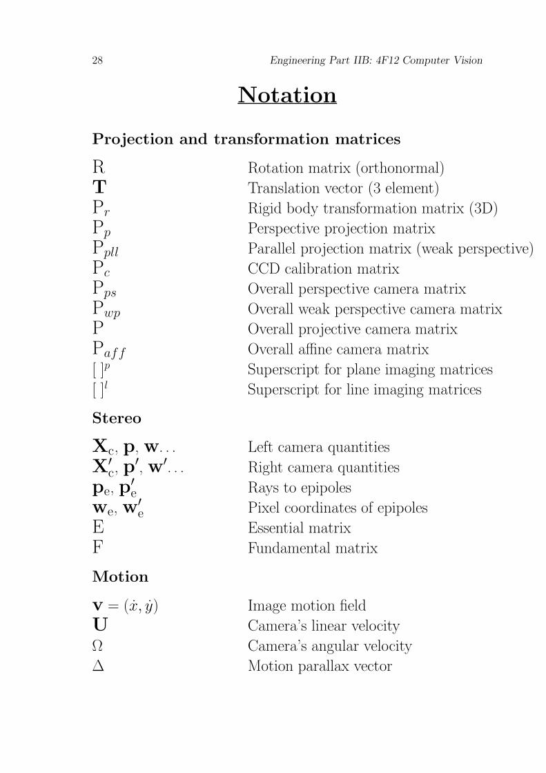
Notation

Projection and transformation matrices

R Rotation matrix (orthonormal)

T Translation vector (3 element)

Pr Rigid body transformation matrix (3D)

Pp Perspective projection matrix

Ppll Parallel projection matrix (weak perspective)

Pc CCD calibration matrix

Pps Overall perspective camera matrix

Pwp Overall weak perspective camera matrix

P Overall projective camera matrix

Paff Overall affine camera matrix

[ ]p Superscript for plane imaging matrices

[ ]l Superscript for line imaging matrices

Stereo

Xc, p, w. . . Left camera quantities

X′c, p

′, w′. . . Right camera quantities

pe, p′e Rays to epipoles

we, w′e Pixel coordinates of epipoles

E Essential matrix

F Fundamental matrix

Motion

v = (x, y) Image motion field

U Camera’s linear velocity

Ω Camera’s angular velocity

∆ Motion parallax vector

university of cambridge engineering part iib module...

Documents