university of groningen quantitative assessment of english
TRANSCRIPT

University of Groningen
Quantitative assessment of English-American speech relationshipsShackleton Jr., Robert George
IMPORTANT NOTE: You are advised to consult the publisher's version (publisher's PDF) if you wish to cite fromit. Please check the document version below.
Document VersionPublisher's PDF, also known as Version of record
Publication date:2010
Link to publication in University of Groningen/UMCG research database
Citation for published version (APA):Shackleton Jr., R. G. (2010). Quantitative assessment of English-American speech relationships. [s.n.].
CopyrightOther than for strictly personal use, it is not permitted to download or to forward/distribute the text or part of it without the consent of theauthor(s) and/or copyright holder(s), unless the work is under an open content license (like Creative Commons).
The publication may also be distributed here under the terms of Article 25fa of the Dutch Copyright Act, indicated by the “Taverne” license.More information can be found on the University of Groningen website: https://www.rug.nl/library/open-access/self-archiving-pure/taverne-amendment.
Take-down policyIf you believe that this document breaches copyright please contact us providing details, and we will remove access to the work immediatelyand investigate your claim.
Downloaded from the University of Groningen/UMCG research database (Pure): http://www.rug.nl/research/portal. For technical reasons thenumber of authors shown on this cover page is limited to 10 maximum.
Download date: 22-11-2021
Chapter 2
Phonetic Variation in theTraditional English Dialects:a Computational Analysis
Abstract. This article illustrates the utility of a variety of quantitative tech-niques by applying them to phonetic data from the traditional English dialects.The techniques yield measures of variation in phonetic usage among Englishlocalities, identify dialect regions as clusters of localities with relatively similarpatterns of usage, distinguish regions of relative uniformity from transitionalzones with substantially greater variation, and identify regionally coherentgroups of features that can be used to distinguish some dialect regions. Com-plementing each other, the techniques provide a reasonably objective methodfor classifying at least some traditional English dialect regions on the basis ofcharacteristic features. The results largely corroborate standard presentationsin the literature but di�er in the placement of regional boundaries and identi-�cation of regional features, as well as in placing those systemic elements in abroader context of largely continuous and often random variation.1
2.1 Introduction
In the 130 years since Wenker's collection of German data inaugurated thesystematic study of dialect variation, scholars have extended the repertoire of
1The �nal, de�nitive version of this paper has been published in the Journal of EnglishLinguistics, Vol. 35, No. 1 (March 2007) by SAGE Publications, Inc. All rights reserved.©2007. On-line version available at http://eng.sagepub.com/cgi/content/abstract/35/1/30.
13

14 CHAPTER 2. THE TRADITIONAL ENGLISH DIALECTS
recording and analytic techniques far beyond the impressionistic collection andcompilation of dialect features and the identi�cation of isoglosses. Over thepast generation, quantitatively oriented researchers have laid the foundationsof a discipline of computational dialectology, providing a set of quantitativetechniques that can be used to address a wide range of issues in languagevariation: Can useful metrics be developed to measure di�erences in speakers'phonetic, lexical, and syntactic usages in di�erent locations � or, by extension,in di�erent social groups, or at di�erent periods? How does individual vari-ation in language use compare with variation among speakers of the �same�dialect, and how does the latter compare with variation among speakers of �dif-ferent� dialects? Is regional dialect variation largely random, or geographicallycontinuous, or can the continuum reasonably be divided into dialect areas withrelatively distinct boundaries? Is it possible to distinguish core dialect regionswith relatively uniform patterns of usage from transitional zones with greaterdiversity? Can dialect regions be characterized by systematic variations infeatures, such as chain shifts or devoicing of voiced consonants; and if so, whatfeatures distinguish a given dialect region from neighboring areas? Can a stan-dard language be traced to origins in geographically restricted dialects? All ofthose issues can be explored through the application of quantitative techniquesto dialect data.
As a general rule, quantitative methods are simply ways of characterizingobservations of interest as variable quantities, of teasing out patterns of corre-lation among variable observations, or of isolating groups of similarly varyingobservations, thereby reducing variation along a large set of relevant dimen-sions to variation along a smaller set. Such methods can therefore be used toexplore the questions posed above by characterizing linguistic data as quanti-ties; by establishing measures of linguistic di�erence � gauges of the degree ofaggregate similarity between speakers' linguistic usages; by classifying speakersinto groups on the basis of similarity; and by grouping linguistic features on thebasis of their distributions among speakers � in short, by quantifying linguisticvariation and uncovering patterns of variation that are both linguistically andstatistically signi�cant.
Some quantitative tools, such as multiple regression and analysis of vari-ance, can be used to explain or predict variation in a linguistic phenomenonof interest on the basis of variation in several other phenomena. Such toolsare often used in conjunction with the assessment of explicit models usingtests of statistical signi�cance and so forth. Other multivariate techniques,such as cluster analysis, multidimensional scaling, or principal component andfactor analysis, are used to summarize and explore interrelationships amongsets of variables more generally, and are less typically used in conjunction withstatistical tests of speci�c models.2
2For readers seeking non-technical summaries, Bartholomew et al. (2002) and Tabachnick

2.1. INTRODUCTION 15
To the extent that quantitative methods help researchers identify dominantpatterns by eliminating dimensions of variation in the data, they also resultin a loss of information because generally speaking, not all of the variationcan be summarized in a smaller number of dimensions. The methods thereforetypically involve a trade-o� between completeness of information and simplicityand interpretability of results. In the study of linguistic variation, they ofteninvolve a trade-o� between capturing broad patterns of relatively systematicvariation and preserving information about relatively minor ones.
Although most of the techniques discussed here can be applied to a widerange of data, a few are drawn from the study of genetic variation. Linguisticand genetic systems present similar mathematical problems despite the di�er-ences in their underlying processes of production, maintenance, and change.Like historical linguists, geneticists face the problem of inferring historical re-lationships among information systems that are replicated with error, that arecomposed of units that can be favored and selected by chance, mutual inter-action, or environmental pressure, that therefore gradually change over time,and that may have geographic distributions that provide insights into theirhistorical development.3 Linguists may therefore �nd useful applications forsome of the algorithms used to measure genetic distances between species, toinfer the historical development of groups of related species (that is, their phy-logenies), and to isolate important geographic boundaries between distinctivegroups.
The �eld of computational dialectology is expanding so rapidly on inde-pendent fronts that no current comprehensive introduction to the full range ofquantitative techniques or their application to linguistic data exists.4 To illus-trate their usefulness I provide a series of applications to phonetic data from
and Fidell (2000) both provide straightforward introductions to the use of speci�c univariateand multivariate techniques. Statistical analysis of linguistic survey data is discussed in detailby Kretzschmar and Schneider (1996).
3A useful standard textbook treatment of phylogenetic techniques can be found in Neiand Kumar (2000). For an interesting example of collaboration between geneticists andlinguists see Nakhleh et al. (2005).
4For the measurement of dialect di�erences � or dialectometry � Heeringa (2004) providesthe most comprehensive English-language review. The Salzburg University DialectometryProject provides a useful online discussion of various aspects of dialectometry, such as di�er-ent measures of similarity, dispersion, and classi�cation, at http://ald.sbg.ac.at/dm/Engl/default.htm. The development of dialectometry (as well as the coining of the term) datesto 1973, when Jean Séguy introduced a simple distance measure in the Atlas Linguistiquede la Gascogne. Hans Goebl (1982) independently developed a similar approach and hassince contributed major advances in broadening the application of quantitative and mappingtechniques to variation among Romance dialects. In North America, Nerbonne (forthcom-ing) and Nerbonne and Kleiweg (2003) have applied dialectometric techniques to data fromthe Linguistic Atlas of the Middle and Southern Atlantic States (LAMSAS), while Labovet al. (2006) and Clopper and Paolillo (2006) have applied related computational techniquesin the classi�cation of North American dialects.

16 CHAPTER 2. THE TRADITIONAL ENGLISH DIALECTS
the traditional dialects of England, highlighting strengths and weaknesses ofdi�erent tools.5
� I construct data sets that quantify variation in the dialects, and use thedata to construct measures of linguistic distance, thereby establishingdegrees of di�erence among speakers in di�erent localities.
� I apply clustering and phylogenetic methods to those linguistic distancemeasures to classify localities into dialect regions of varying coherence.
� I then use regression analysis and barrier analysis to explore the rela-tionship between geographic and linguistic distances within and amongthe dialect regions.
� Finally, I apply principal component analysis to identify groups of pho-netic variants and features that can arguably be said to distinguish someof the dialect regions.
Any parsing or quanti�cation of a coding system as complex as naturallanguage is necessarily somewhat arbitrary � even native speakers, whose per-ceptions might be considered the standard against which to compare any othermeasure, will typically di�er in their assessment of di�erences between dialects� and the patterns of variation uncovered by the use of such measures dependin part on the choice of segments and the choice of measure. Nevertheless, theanalyses yield relatively robust patterns that appear repeatedly under signi�-cantly di�erent approaches and that are likely to represent real and signi�cantpatterns of dialect variation. The results provide strong quantitative evidencefor regions of relatively uniform use of distinctive features as well as othersof substantially greater than average variation, while placing both against abackground of largely continuous variation.
2.2 Data: Survey of English Dialects and Struc-
tural Atlas of English Dialects
The primary data source is Orton and Dieth's (1962) Survey of English Dialectsor SED, the best broad sample of the most traditional forms of rural English
5Other researchers have applied similar techniques to morphological, syntactic, and lexicalvariants in the traditional English dialects. Viereck and Ramisch (1997) include a numberof such studies, including cluster analyses by Goebl, multidimensional scaling by Embletonand Wheeler, and principal component analyses by Inoue and Fukoshima. However, to myknowledge such methods have not been systematically applied to English phonetic variation.An obvious signi�cant extension would be to apply the techniques to an extended data setthat includes the lexical, morphological, and syntactic variants enumerated by (Viereck andRamisch, 1991, 1997).

2.2. DATA 17
dialect that were still in use in the mid-20th century.6 Focusing their resourceson recording the most recessive features of the language, SED �eldworkers in-terviewed a handful of elderly people � mainly men, who were considered morelikely to use nonstandard traditional speech � in each of 313 relatively evenlyspaced, mainly small, rural agricultural communities throughout England, us-ing questionnaires, diagrams, pictures, and spontaneous conversation to elicitresponses. In choosing locations, they gave some consideration to geographicfeatures � mountainous terrain, rivers, and so forth � that were likely to in�u-ence linguistic di�erences among localities. As a consequence, the SED datais a highly representative sample of an important dimension of variation inmid-20th century English dialects, though it should not be considered repre-sentative of variation across other equally relevant dimensions, such as age orsocioeconomic status.
The SED responses were recorded impressionistically, using the 1951 revi-sion of the International Phonetic Alphabet.7 The SED material is presentedby locality, with a county name and number � e.g., Northumberland 1 � as il-lustrated in Figure 2.1 and Table 2.1. Geographic coordinates for each localityin the SED are taken from the United Kingdom's Ordnance Survey website.8
All the results from a given locality are presented together, making it impos-sible to distinguish the responses of individual informants. The responses inthe SED thus represent an aggregated sample of the speech habits of a partic-ular locality rather than those of a particular individual and will be referredto accordingly.9 Where the SED presents more than one form of a word fora locality, I select the �rst unless another form is speci�cally referred to as�older� or �preferred.�
In addition to data taken directly from the SED, I take derived data fromAnderson's (1987) A Structural Atlas of the English Dialects or SAED, whichpresents a series of more than 100 maps showing the geographic distribution
6The systematic study of English dialects is well into its second century, building on thefoundations of Ellis (1889) and the examples of the continental European and Americanlinguistic surveys. Many studies have drawn on the SED for source material, includingimportant introductions to English dialects such as (Wells, 1982a,b) and Trudgill (1999); theatlases by Kolb et al. (1979), Anderson (1987), Upton et al. (1987), Upton and Widdowson(1996), and (Viereck and Ramisch, 1991, 1997). Sanderson and Widdowson (1985) providea historical review of English dialect research, as well as a very useful discussion of the SED.The data used in this study is available from the author upon request.
7Speakers were also tape-recorded in nearly all the localities and in principle their speechcould be studied through a rigorous acoustic analysis.
8The geographic coordinates are freely available online at http://www.ordnancesurvey.co.uk/oswebsite/freefun/didyouknow/.
9The degree of variation bears emphasis: even in localities that appear as the most repre-sentative of their respective regions in the present analysis, it is common to �nd two or threesometimes quite di�erent variants in use in a given set of words in a given locality. Com-petition among variants is especially apparent in areas where regions of generally di�erentusage come into contact.

18 CHAPTER 2. THE TRADITIONAL ENGLISH DIALECTS
Figure 2.1: Localities of the Survey of English Dialects
Source: Orton, Harold. 1962. Survey of English Dialects: An Introduction. Leeds,UK: E. J. Arnold. Reproduced by the permission of the University of Leeds.

2.2. DATA 19
Table 2.1: Traditional Counties in the Survey of English Dialects
1. Northumberland 15. Herefordshire 28. Hertfordshire2. Cumberland 16. Worcestershire 29. Essex3. Durham 17. Warwickshire 30. Middlesex4. Westmoreland 18. Northamptonshire 31. Somerset5. Lancashire 19. Huntingdonshire 32. Wiltshire6. Yorkshire 20. Cambridgeshire 33. Berkshire7. Cheshire 21. Norfolk 34. Surrey8. Derbyshire 22. Su�olk 35. Kent9. Nottinghamshire 23. Monmouthshire 36. Cornwall10. Lincolnshire 24. Gloucestershire 37. Devonshire11. Shropshire 25. Oxfordshire 38. Dorsetshire12. Sta�ordshire 26. Buckinghamshire 39. Hampshire13. Leicestershire 27. Bedfordshire 40. Sussex14. Rutland
and frequency of occurrence of di�erent phonetic variants in groups of wordsfound in the SED, where all of the words in a given group include a segmentthat is posited to have taken a single uniform pronunciation in an older formof the language � the �standard� Middle English dialect of the Home Countiesof southeastern England. The groups include all of the Middle English shortand long vowels, diphthongs, and most of the relatively few consonants thatexhibit any variation in the English dialects. Although it is by no means com-plete or comprehensive, the data set reduces an enormous amount of phoneticinformation to a tractable form that makes possible a rapid and wide-ranginganalysis of phonetic variation in the traditional dialects of England as theyexisted in the middle of the 20th century.
To provide a somewhat broader perspective on the traditional English di-alects recorded in the SED, I expand the data set to include the pronuncia-tions of three idealized speakers: a speaker of the Middle English �standard�on which the SAED classi�cation of localities' responses is based; a speakerof mid-20th century Received Pronunciation; and a speaker of my own na-tive speech pattern, the �Western Reserve� dialect of northern Ohio, whichwas chosen by American radio broadcasters in the early 20th century as mostclosely representing an American standard. More di�cult but very enlight-ening extensions would include data from other regions � Scotland and otherEnglish-speaking countries � and from speakers from a wider range of ages andsocioeconomic backgrounds.

20 CHAPTER 2. THE TRADITIONAL ENGLISH DIALECTS
2.3 Converting Linguistic Data to Quantities:
Variants and Features
Phonetic data can be quanti�ed in a number of useful ways: by classi�cationinto sets of variant phonemes, by perception- or articulation-based measure-ment of features such as vowel height and backing, or by measurement of acous-tic features through spectrograms and formant tracks. Using such approaches,distances between two speakers' phonemes or segments can be measured asdi�erences between their variants, articulatory features, or acoustic features.Detailed analysis by Heeringa (2004) suggests that no such approach providesan ideal quanti�cation of speech, but that measures of di�erences betweenspeakers based on them are fairly closely and similarly correlated with nativespeakers' perceptions of those di�erences, at least in the aggregate.10
I take two distinct approaches to quantifying the SED data for this analysis.One quanti�es a small number of mainly vocalic phonemes in SED responsesinto sets of features, such as degrees of height, backing, and rounding. Theother approach is based on the SAED 's classi�cation of a much larger set ofSED responses into sets of phonetic variants � for instance, the use of [ou],[o@], [ia], etc., in words typically pronounced like bone. The feature-basedapproach makes possible a detailed analysis of subtle variation in a small setof responses; the variant-based approach permits a rapid analysis of a largenumber of responses with comparatively little e�ort. Comparing the resultsof the two approaches yields further understanding of their relative strengthsand weaknesses and of dialect variation in general. Although comparison ofstrings of segments such as words or phrases would provide further insight, theanalysis considers only short segments in the interests of economy.
On the whole, these approaches almost certainly considerably understatethe full extent of phonetic variation among the localities in the SED � thefeature-based approach because it is based on such a small set of phonemes,the variant-based approach because its classi�cations obscure a great deal ofvariation. That understatement simpli�es the use of various algorithms touncover structure, but to such an extent that a skeptic may reasonably wonderwhether the results are not due mainly to the choice of classi�cations and wordsthan to the use of quantitative tools. Despite their limitations, however, bothdata sets faithfully record a wide range of variation. Moreover, the sourcesof understatement do not appear likely to result in any other systematic biasin the measurement of dialect di�erences. As a result, the distance measures,clusters, and factors uncovered in this study appear likely to be relativelyrobust to improvements in the measurement of true variation.
10See especially Heeringa (2004), Chapter 7, Section 4.3.

2.3. VARIANTS AND FEATURES 21
2.3.1 Feature-Based Approach: Quanti�cation
The feature-based approach closely analyzes a set of 55 words shown in Ta-ble A.1 in Appendix A. The set includes at least one example of every shortvowel, long vowel, and diphthong in �standard� Middle English, alone and fol-lowed by rhotics, as well as the variable consonants. The approach translates122 segments (including vowels, diphthongs, and consonants) into vectors ofnumerical values representing 483 features such as degrees of height, backing,and rounding. That translation � necessarily a somewhat arbitrary process �provides numerical characterizations that can be used to calculate a measureof perceptual or articulatory distance between segments.
According to the approach I adopt here � of my construction but similarto the system of Almeida and Braun (1986) � short and long vowels are repre-sented as vectors of four values: 1.0 to 7.0 for height, 1.0 to 3.0 for the degree ofbacking, 1.0 to 2.0 for rounding, and 0.5 to 2.0 for length. Thus, for instance,[a] takes values of [1.0, 1.0, 1.0, 1.0] while [u:] takes values of [7.0, 3.0, 2.0,2.0]. I ignore most diacritics. Diphthongs are represented by a vector of eightnumbers; for example, [ou] and [o:@] would take values of [5.0, 3.0, 2.0, 1.0,7.0, 3.0, 2.0, 1.0] and [5.0, 3.0, 2.0, 2.0, 4.0, 2.0, 1.0, 0.5], respectively. Forsome types of analysis, I convert the values describing the second element ofa diphthong to di�erences between the second element and the �rst. For thediphthongs above, for example, the values would be [5.0, 3.0, 2.0, 1.0, 2.0, 0.0,0.0, 0.0] and [5.0, 3.0, 2.0, 2.0, -1.0, -1.0, -1.0, -1.5], respectively. If monoph-thongs are assigned values of 0.0 for the second set of features, monophthongsand diphthongs can both be included in a square matrix, with the second setof features representing the characteristics of the glide. This second approachmakes possible a novel analysis of variations in glide characteristics in the prin-cipal component analysis described below. Consonants are represented by avalue representing the presence or absence of the relevant distinctive feature;rhotics are represented by two values representing the place and manner of ar-ticulation.11 I also tabulate data on whether multiple responses were recordedin a given locality.
11Rhotics are assigned values for place and manner of articulation consistent with theInternational Phonetic Alphabet as in the system of Almeida and Braun (1986): the uvulartrill [K] is assigned a value of 9 for place and 3 for manner; alveolar trill [r] is assignedvalues of 3 and 4, respectively; alveolar approximant [ô] is assigned values of 7 and 4, andretro�ex tap/�ap [ó] is assigned values of 4 and 6. The absence of a rhotic is assigned aplace value intermediate between postalveolar and retro�ex (5.5) and a manner value of 9.This approach thus places signi�cant emphasis on the presence and realization of rhotics.

22 CHAPTER 2. THE TRADITIONAL ENGLISH DIALECTS
2.3.2 Feature-Based Approach: Distribution and Corre-
lations
Only 447 of the features have any variance; the remaining 36 are constantacross all localities. That each word has its own history is underlined by thefact that the means and standard deviations of vowel features are distributedmore or less uniformly; that is, for any given feature � vowel height, for example� the mean value across localities for any given word is unique, and the meanvalues for all words show no distinctive pattern at all. Even features of thevowels in words as similar as sun and butter have noticeably di�erent meansand standard deviations. However, feature distributions reveal an importantunderlying pattern. For every feature, high standard deviations strongly tendto be associated with middling feature values, while low deviations are asso-ciated with extreme values; that is, low or high vowels tend to have fairlyuniform distributions across speakers. A low (or high) vowel typically is low(or high) in most localities, and so the standard deviation of its distributiontends to be low. In contrast, vowels of medium height tend to have variedexpressions across dialects and high standard deviations in their distributions.The same observation holds for backing, rounding, and length, but the pat-tern has di�erent causes in di�erent cases. For some features, including vowelheight, it arises from the fact that the position of middling vowels such as[E] and [O] is quite variable � that is, that middling vowels tend to be ratherunstable. In the case of rounding and length, however, it is due mainly to thefact that features with average values closer to the mean are simply those forwhich many localities use a rounded or short variant while many others use anunrounded or long one.
Relatively few features are closely correlated. Only about two percent ofall Pearson correlations between features have an absolute value greater than0.5, and only about 15 percent are greater than 0.25. The typical feature willhave a correlation with absolute value of 0.5 or more with only a dozen otherfeatures. However, those averages mask a great deal of variation in the degreeof correlation among features. About a quarter of the features have no morethan two correlations with absolute value greater than 0.5, but roughly anotherquarter have correlations that high with 20 or more other features. On closerexamination, the highly correlated features turn out to be composed largely ofthree classes � one composed of fricatives, which all tend to be voiced in theSouthwest; another composed of features of second segments of diphthongs,which tend to develop inglides in the North and upglides in the Southeast;and a third composed of rhotic features or, in the non-rhotic dialects, theirreplacements.

2.3. VARIANTS AND FEATURES 23
2.3.3 Variant-Based Approach: Quanti�cation
In the variant-based approach, I use data from the SED and SAED to cal-culate localities' frequencies of usage of groups of phonetic variants (mainlyof vowels) in groups of words believed to have had uniform pronunciations in�standard� Middle English. The variant-based data set summarizes over 400responses, grouping them into 199 variants of 39 phonemes or combinations ofphonemes.12 The full set of groups of variants is shown in Table A.2 in Ap-pendix A; the words used appear in the index of the SAED. (Throughout therest of the presentation, I write the Middle English form considered common� not to say ancestral � to the group as /x/ and the variants recorded in theSED as [x].)
The typical map from the SAED shown in Figure 2.2 illustrates strengthsand weaknesses of both the data and the approach. The map shows approx-imate frequencies of use in SED localities of variants closely approximating[@i], [ei], or [Ii] � that is, rising diphthongs with a centered, center-front, orslightly higher than center-front onset � in a set of 20 words, such as cheeseand geese, believed to have been pronounced with /e:/ by speakers of �stan-dard� Middle English.13 A closer examination of the SED material revealsthat the variants in question are not used uniformly in the di�erent regions:localities in the Southeast and East Anglia uniformly use [Ii]; those in theNorthwest Midlands tend to use [Ei] or [Ei] but occasionally [Ii], and those inNorth Yorkshire typically use [ei] or [@i] but also occasionally [Ii]. In this case,then, the responses can be classi�ed further into three separate groups on thebasis of di�erences both geographical and linguistic. (In a few cases, localitiesfrom geographically separate regions are classi�ed as having �di�erent� vari-ants even though the variants are actually the same, on the grounds that thevariant is likely to have arisen independently in the two regions. For instance,localities in the North who use [i: ∼ e:] in words with /E:/ in Middle Englishare distinguished from those in the South and Midlands who use the samevariant, since there is a large geographic gap between the regions in which thevariant does not appear at all.)
I also translate the variants described in Table A.2 into vectors of numericalvalues representing features. In contrast to the �rst feature-based approach, I
12The addition of standard Middle English also requires the addition of 10 variants thatwere no longer in use in any of the localities under study in the twentieth century; thevariants identi�ed for Received Pronunciation and Western Reserve were all in use in atleast a few localities.
13Because the maps present only ranges of frequencies, I use the averages of those ranges(i.e. 92.5 percent for speakers with frequencies between 85 percent and 100 percent). Thatapproach also requires that each locality's frequencies be normalized to sum to 1.0 over eachset of words that are held to share a phoneme in Middle English (since they may not do soautomatically) and introduces a layer of error to the data that should be of relatively littleconsequence for the analysis.

24 CHAPTER 2. THE TRADITIONAL ENGLISH DIALECTS
Figure 2.2: A Typical Map from the Structural Atlas of English Dialects
Source: A Structural Atlas of the English Dialects, Peter Anderson, Copyright 1987Croom Helm Ltd. Reproduced by permission of Taylor and Francis Books UK.

2.3. VARIANTS AND FEATURES 25
represent short monophthongs as a vector of three numbers representing height,backing, and rounding; long monophthongs and diphthongs are represented bya vector of six values. The treatment of consonants and rhotics follows thefeature-based approach. Where a variant in Table A.2 actually represents arange of distinguishable sounds, its characterization generally takes the meanvalue for each feature over the range of sounds assigned to the speci�c variantin the SAED. As in the feature-based approach, I ignore most diacritics.
The classi�cation of words into groups imposes several limitations. It tendsto understate the true extent of variation in several ways and, by precludingthe pairwise comparison of individual words or phonemes in words, limits therange of approaches that can be used to analyze that variation. A historicalbasis for grouping words together is as compelling as any other approach, butthe words may not in fact have been pronounced the same even in �standard�Middle English, in which case they may be inappropriately grouped even onthe stated basis. In addition, speci�ed variants often comprise a range ofdistinguishable sounds � such as [@i], [ei], and [Ii] in the example above � thusmasking a signi�cant amount of variation. Similarly, even informants usingtraditional speech forms in a given locality may have substantially di�erentusage that is masked by the presentation of the SED material by locality.Perhaps more importantly, two localities' usage may di�er considerably acrossa given group of words even if they have identical frequencies of use of eachvariant. In the extreme, one can imagine two localities using each of twovariants for 50 percent of the words, but using di�erent variants for each word.Conversely, of course, the approach also may tend to overstate the true extentof variation in some cases, as when two localities may use the same variant (forinstance, [Ii] in the example above) but be classi�ed as using di�erent variants.Nevertheless, as mentioned above, the approach also has the advantage ofallowing the rapid analysis of a large set of responses.
2.3.4 Variant-Based Approach: Distribution and Corre-
lations
The full distribution of variants resembles the asymptotic hyperbolic (or �A-curve�) distribution discussed by Kretzschmar and Tamasi (2002) as beingcommon to dialect data: a small set of the variants in the data set accounts formost usage while the minority has relatively limited distributions. The averagevariant is used in about 20 percent of all localities, but 29 variants (about 15percent of the total) are used in 50 percent or more of all localities, while 73(about 36 percent) are used in �ve percent or fewer. Ignoring variations in thefrequency of occurrence of di�erent phonemes, 25 variants account for nearlyhalf of all usage across all phonemes, while the least common 115 variantsaccount for only 10 percent.

26 CHAPTER 2. THE TRADITIONAL ENGLISH DIALECTS
Most variants have a relatively unique distribution among and frequencyof use within SED localities. The distributions of variants may overlap a greatdeal � even the distributions of variants of the same phoneme � but they rarelyentirely coincide. This can be seen most clearly in the Pearson correlationsbetween variants. Only about three percent of all the Pearson correlationsbetween variants are greater than 0.5, and only about 11 percent are greaterthan 0.25. Those values imply that the typical variant will have a correlationof 0.5 or more with only �ve or six other variants and a correlation of 0.25or more with only about 20 of them. However, those averages mask a greatdeal of variation in the degree of correlation among variants. Most variantshave very few large correlations with others: 53 variants have no correlationsas large as 0.5, and 95 variants have three or fewer. In contrast, 25 variantshave 15 or more correlations of 0.5 or greater and 35 variants have 12 or more.Interestingly, most of the variants with a large number of large correlations arefound either in the far Southwest or in the far North of England. That �ndingsuggests that those two regions tend to have relatively distinctive speech formswith numbers of features that regularly co-occur in them, exempli�ed, forinstance, by the very similar geographic distributions of voiced fricatives inthe Southwest.
With the exception of the extensive correlation of a relatively small groupof variants, the typically low levels of correlation among variants provide strongevidence that most variants do not tend to co-occur very regularly with manyothers. That observation, in turn, implies that localities in the SED may sharespeci�c variants in common but are unlikely to share overall patterns of usage,and provides support for the view of dialect variation as a largely continuousphenomenon.
At the same time, the correlations among variants provide a number ofclues as to the extent of systematic structural variation among the speechvarieties in SED localities. The most obvious example is fricative voicing inthe Southwest; but perhaps the most notable instance is the set of positivecorrelations between parallel developments in the Middle English front andback low long vowels shown in Table 2.2. In much of the North of England, thevowels tend to merge with great regularity. In other parts of the North, theyboth tend to develop inglides. In parts of the North Midlands, they are simplyraised, and the degree of raising tends to be correlated. Finally, the vowels bothdevelop upglides in most of the South, and where they do, the heights of theinitial vowels in the resulting diphthongs tend to be similar. The co-evolutionof the low front and back vowels thus appears to be a genuinely structuraldevelopment in the English dialects. Note, however, that in most of thosecases the correlations between parallel developments, while positive, are notespecially large: the structural parallels appear to be at least partly systematicin nature but may perhaps best be interpreted as statistical tendencies rather

2.3. VARIANTS AND FEATURES 27
Table 2.2: Correlations between Developments in Front and Back Long Vowels
Middle English Middle English/a:/ develops to: Correlation: /O:1/ develops to:
[i@] 0.8940 [i@ ∼ e@ ∼ E@]a
[iE ∼ jE] 0.7883 [iE ∼ jE ∼ ji]a
[ia ∼ ea] 0.9114 [ia ∼ ea]a
[e@ ∼ E@]b 0.6488 [u@ ∼ o@ ∼ 2u@ ∼ O@ ∼ o:@][e:] 0.5987 [o:][i:] 0.4690 [u: ∼ u: ∼ Y:]
[ei ∼ e:i] 0.3075 [ou][Ei ∼ E:i] 0.5003 [Ou ∼ 6o ∼ u][æi ∼ ai] 0.5032 [@u ∼ 2u ∼ æu]
a - In medial position.b - In Yorkshire and Lincolnshire.
than strict relations.In other cases, the correlations among variants reveal some proposed dialect
structures to be largely chimerical. For example, the �Potteries� dialect ofnorth Sta�ordshire and surrounding counties has been characterized by thefollowing pronunciations:14
� Bait and bate are pronounced [bi:t]; that is, Middle English /a:/ and/ai/ merge and develop to [i:].
� Beat and beet are pronounced [bEit] � Middle English /E:/ and /e:/merge and develop to [Ei].
� Boat is pronounced [bu:t] or [bY:t] � Middle English /O:1/ or /O:2/develop to [u: ∼ Y:].
� Boot is pronounced [bEUt] � Middle English /o:/ develops to [EU].
� Bout is pronounced [bait] � Middle English /u:/ develops to [ai].
� Bite is pronounced [bA:t] � Middle English /i:/ develops to [A:].
� Bought is pronounced [bout] � Middle English /ou/ remains or revertsto [ou].
14See for example Trudgill (1999), p. 41. Trudgill attributes this characterization to thespeech of all of Sta�ordshire plus parts of Cheshire, Shropshire, Derbyshire, Warwickshire,and Worcestershire.

28 CHAPTER 2. THE TRADITIONAL ENGLISH DIALECTS
� Caught is pronounced [koUt] � Middle English /au/ develops to [oU].
All of the variants are indeed found in SED localities in north Sta�ordshire,Cheshire, and Derbyshire in words from the 11 relevant Middle English wordgroups. However, a close inspection reveals that no SED locality uses themall; only two localities use the variants in 9 of 11 groups, and 6 other localitiesuse 7 or 8. Taking into consideration frequency of use over the range of wordsin each group, the highest-scoring locality, Sta�ordshire 3, uses the �Potteries�variants in 60 percent of the possible occurrences, and only 8 localities use themin more than one-third of possible occurrences. Moreover, further analysis ofthe variants' frequencies of occurrence reveals that many of their correlationsare relatively weak, even in the relevant region. Viewed in terms of correlationsbetween variants and frequencies of use in the SED material, actual �Potteries�usage, even among traditional dialect speakers of the mid-twentieth century,appears to be more of a tendency to use certain variants with greater frequencyrather than a coherent, distinct linguistic structure.
Taken altogether, the patterns of correlation among features and amongvariants suggest two important insights into the patterns of variation in thetraditional English dialects. First, with the exception of the distinctive shiftsof the far North and the far Southwest, phonetic variation in the dialects issimply not very systematic, but instead tends to involve largely uncorrelatedvariations that, in some areas, coalesce into patterns that appear more system-atic. Second, most of the phonetic variation tends to involve single featuresrather than combinations of features. Even when groups of correlated featuresappear to indicate greater structural variation, the structural shift involvedtends to be fairly simple: rhotic type, voicing or devoicing, or upglides versusinglides in diphthongs.
2.4 Calculating Linguistic Distances
A variety of measures can be used to quantify the di�erence between speci�cusages of one speaker or locality and another and to aggregate large numbers ofsuch di�erences into a single quantity, although none of them should be takenas a perfectly accurate gauge. For variants, for example, distances betweenspeci�c phonetic segments can be taken as 0 for speakers with the same variantor 1 for speakers with di�erent variants. For feature-based characterizations ofsegments, distances can be calculated using such measures as Manhattan �city-block� distance or Euclidean distance. (For instance, the Manhattan distancebetween [E] and [u] is 7.0; the Euclidean distance 4.6.) Such measures canbe converted to logarithms � in this case, 1.95 and 1.53, respectively � on theargument that small di�erences have a relatively greater perceptual distanceand should be given greater weight relative to larger ones.

2.4. CALCULATING LINGUISTIC DISTANCES 29
Any measure of distance between segments can be extended to whole wordsor utterances using the more complex Levenshtein distance, which is de�nedas the minimum cost of changing one word or utterance into another by meansof insertions, deletions, and substitutions of one segment for another.15 TheLevenshtein distance is extremely useful for comparing dialects but requiresthe coding of entire words rather than individual segments. I therefore focuson segment-based measures instead.
2.4.1 Segments
To calculate a linguistic distance between segments, I introduce a somewhatnovel measure of Euclidean distance between the articulation-based numericalcharacterizations of segment features. The variant-based and feature-basedapproaches di�er slightly. In the variant-based approach, the distance calcula-tion is generally intended to re�ect the number of changes that have occurredsince the variants diverged from an ancestral monophthong or diphthong, sothat the approach taken depends on the nature of both descendant variantsand that of the inferred ancestral vowel. If both variants are of the same type,the distance calculation is straightforward. If one variant is short and the otherlong or a diphthong, the distance is generally calculated over the characteris-tics of the short variant and of the �rst element of the long variant, plus 1.0for the lengthening or the diphthong's additional element in the diphthong.For example, the di�erence between [e] and [i:] is 1.414 � the square root ofthe sum of 1.0 for the distance between [e] and [i] plus 1.0 for lengthening.Matters get more complicated still if some descendents of an ancestral shortor long phoneme have developed inglides and others o�glides, as for examplewith Old English [o:] developing to [i@] in some northern dialects and to [Ui]in parts of West Yorkshire. In this case, I calculate the distance between thefeatures of the second element of the �rst diphthong and those of the �rst ele-ment of the second one, adding 2.0 for the addition of an inglide in the formerand an upglide in the latter. I make analogous adjustments for other complexcomparisons, such as between shortened and diphthongized descendants of alengthened ancestral vowel. I generally give a value of 1.0 to distances betweenvariants of consonants (which usually involve voicing or devoicing) except inthe case of the various rhotics, where I calculate a Euclidean distance betweentwo-element vectors representing place and manner of articulation.
The feature-based approach di�ers from the variant-based approach in
15First introduced into dialectology by Kessler (1995) to measure dialect distances amongspeakers of Irish Gaelic, the Levenshtein distance has become a preferred approach for manyresearchers because of its comprehensiveness and �exibility. The more complex Damerau-Levenshtein distance also accounts for transposition of segments and can therefore addressdialect changes involving extensive metathesis.

30 CHAPTER 2. THE TRADITIONAL ENGLISH DIALECTS
treating all monophthongs as single segments with four variable features, withlength as a feature ranging in value from 0.5 to 2.0. I calculate the distance be-tween a monophthong and a diphthong over the characteristics of the monoph-thong and the �rst element of the long variant plus 1.0 for the di�erence be-tween a monophthong and a diphthong; the distance between diphthongs is astraightforward Euclidean distance calculation over all eight features, ignoringconsiderations of historical development. Consonants and rhotics are treatedas described for the variant-based approach.
2.4.2 Aggregation
Researchers can use a variety of di�erent approaches to aggregate di�erencesbetween localities usages � whether based on perception, articulation, or acous-tics � and to calculate aggregate distance measures, with no approach likelyto yield a perfect measure. The present analysis aggregates feature-based Eu-clidean distances by taking the average distance over all 122 segments in thedata set. An aggregate measure of 1.0 thus implies that on average, two lo-calities' phonemes in this set of segments di�er about as much as do [e] and[E] or [o] and [O]. Note that the aggregation does not take into account themany segments that are unvarying across English localities. In that sense, theaggregation procedure greatly exaggerates the �true� degree of distance amonglocalities.
The variant-based approach is generally similar, except for adjustmentsneeded to accommodate localities' varying frequencies of use of several di�erentvariants. In many cases, localities may share some variants in common butnot others, but by construction the data obscures the extent of word-by-wordoverlap. Localities with the same frequency of use of a particular variant mayor may not use them in the same words. Since there is no way to determine thedegree of overlap between them short of comparing them word by word, theanalysis simpli�es the process by assuming that shared frequencies of a givenvariant correspond to shared pronunciations in speci�c words (over which thelocalities have zero linguistic distance), distributes the remainder uniformlyamong remaining variants, and calculates distances accordingly.
Table 2.3 shows a simple example in which two speakers each occasionallyuse three di�erent variants over a given set of words (by assumption, only onevariant per word), but with di�erent frequencies of use. Variants 1 and 2 areassumed to have a linguistic distance of 1.5; variants 1 and 3 a distance of 2.0,and variants 2 and 3 a distance of 2.5. For the calculation of linguistic distance,the speakers are assumed to share pronunciations where their frequencies ofuse overlap; that is, they are both assumed to use Variant 1 in 10 percentof the words, Variant 2 in 10 percent, and Variant 3 in 30 percent. For theremaining 50 percent of words, Speaker 1 is assumed to use Variant 2, while

2.4. CALCULATING LINGUISTIC DISTANCES 31
Table 2.3: Calculation of Variant-Based Linguistic Distance: An Illustration
Common RemainderSpeaker 1 Speaker 2 to Both (Speaker 1 �
Frequencies (%) Frequencies (%) Speakers (%) Speaker 2; (%)
Variant 1 10.0 40.0 10.0 �30.0Variant 2 60.0 10.0 10.0 50.0Variant 3 30.0 50.0 30.0 �20.0Total 100.0 100.0 50.0 50.0
Linguistic Distances
Variants 1 & 2 1.5Variants 1 & 3 2.0Variants 2 & 3 2.5
Speaker 2 is assumed to use Variant 1 in 30 percent and Variant 3 in 20percent. The distance calculation between the two speakers is thus 30 percenttimes 1.5 (the distance between Variants 1 and 2) plus 20 percent times 2.5(the distance between Variants 2 and 3), for a total of 0.95. Thus, even thoughthe speakers use three di�erent variants with distances between the variantsranging from 1.5 to 2.5, the reasonable assumption that they very likely shareat least some of those variants in speci�c words reduces their average linguisticdistance over this set of words to somewhat less than 1.0. The approach yieldsthe minimum possible average distance over this set of words, and thereforealmost certainly further understates the actual degree of variation between anytwo SED localities. However, in this respect as with the use of word groups,the approach appears unlikely to result in any other systematic bias in thedistance measurement, and the relative distances among localities are thereforeprobably robust to improvements in the measurement of true variation. Ialso adjust the variant-based linguistic distance by weighting distances forparticular sets of phonemes by the number of words taken by Anderson fromthe SED for each group of words, on the grounds that the relative frequencyin that selection may be a fairly reasonable approximation of the frequency ofoccurrence in traditional general speech.16 With over 400 responses in totaland 39 vowels, diphthongs and consonants, the average phoneme is representedby about 10 tokens, with the number of tokens per phoneme ranging from oneto 33.
In addition to the measures discussed here, one may calculate Pearsoncorrelations for vectors of variant frequencies � more accurately thought of asa similarity measure than a distance measure � or a distance measure used in
16The distance measures are calculated using Fortran-based programs developed by andavailable from the author upon request.

32 CHAPTER 2. THE TRADITIONAL ENGLISH DIALECTS
genetics, such as Nei's distance, which tends to be rather closely correlatedwith the Pearson correlation. Although such approaches have less linguisticfoundation than the feature-based results presented here, they tend to yieldsimilar results.
2.4.3 Results: Feature-Based Distances
The feature-based linguistic distances reveal a wide range of variation amongthe localities in the SED, but as shown in Figure 2.3, the vast bulk of the mea-sured similarities are rather uniform, with nearly 85 percent of the distancesbetween localities falling between 0.7 and 1.4. The average distance across alllocalities is about 1.1. (To put those values in perspective, consider that themaximum distance between short vowels is about 7.3 and between long vowelsor diphthongs is about 10.4, and the distance between two randomly chosenvowels or diphthongs � or between two randomly selected vectors of vowels �is thus likely to be around 4.4.) Relatively few localities are radically di�erentfrom each other, with the largest distances of nearly 1.8 pointing to di�erencesbetween Cumberland 1 on the Scottish border and a number of localities inEast Anglia and the Southwest. Nevertheless, even though neighboring locali-ties are occasionally very similar in their speech forms � the smallest distancepoints to a pair of localities in Somerset that are very nearly identical in theirspeech � similarity appears to be the exception rather than the rule even atrelatively short geographic distances. Only about two percent of the distancesare less than 0.5, implying that the typical locality will be that similar tono more than 6 or 7 other localities. Thus there are relatively few localitiesthat are extremely similar in their speech but also relatively few (mainly thosein Northumberland and Devonshire) that are quite di�erent from the rest ofEngland.
Localities have quite diverse patterns of close similarity. Some localities �mainly those centered in broad regions with relatively uniform speech patterns,such as North Yorkshire, Leicestershire, and western Essex � have linguisticdistances of less than 0.5 with as many as 25 other localities. In contrast,nearly 40 localities, which generally appear to be either genuine outliers suchas Cumberland 1 on the Scottish border or in transition zones between re-gions of relative uniformity (Worcestershire 1, Herefordshire 7, Hertfordshire3, Oxfordshire 2, and Northamptonshire 5 being notable examples) have nofeature-based distances of less than 0.5.
The distance measures are fairly closely correlated with geographic dis-tance, with a Pearson correlation of 0.70 � a strong indication that geographicseparation has played an important role in the development of the traditionalEnglish dialects. One consequence of this fact is that localities in the middleof the country � localities that often tend to have relatively large distances

2.4. CALCULATING LINGUISTIC DISTANCES 33
Figure 2.3: Distribution of Linguistic Distances
with neighboring localities because they are in or near a major transition zonebetween North and South � also tend to have more in common with localitiesat both ends of the country than do speakers at the ends with each other.17
Most of the localities with the lowest average distances with all other localities,ranging just above 0.9, are in the Midlands. In contrast, most of the localitiesthat are relatively distinctive from all other localities are in the Far Northor the Southwest, with Cumberland 1 having the highest average of over 1.4.Standard deviations of distances tend to be highest for localities in the South-west, suggesting that those localities tend to have a wide range of distanceswith other localities, while skewness tends to be highest for localities both inthe Far North or the Southwest.
17Goebl and Schiltz (1997) describe degrees of �skewness� for SED localities on the basisof lexical and morphological characteristics. They show that localities with the same averagesimilarity with other localities may di�er in the distribution of distances from low values tohigh values, so that one is relatively similar to most other localities but very di�erent froma few, while the other is somewhat dissimilar to most but not terribly similar to any. Theyshow that for the linguistic variables they examine, a swath of south-central England hasthe lowest degree of skewness and thus the greatest degree of integration into the dialectcontinuum. In the present study, in contrast, the lowest degree of skewness for localities'phonetically-based linguistic distances occurs in the Midlands, mainly but not invariablyamong those localities that have the lowest average distances.
34 CHAPTER 2. THE TRADITIONAL ENGLISH DIALECTS
Feature-based linguistic distances provide another prism through which toview the �Potteries� dialect region, which remains as indistinct as it was whenanalyzed in terms of variants. If we calculate linguistic distances betweenidealized �Potteries� pronunciations and SED responses for words from therelevant groups � gate, meat, cheese, white, loaf, moon, house, daisy, daughter,and snow � we �nd that localities around north Sta�ordshire have the smallestdistances from the ideal, but that even the localities with the smallest distances� most of them slightly north of Sta�ordshire in Derbyshire, Cheshire, andLancashire � have distances that are about 40 percent as large as the largestdistances.
Data on the occurrence of multiple responses for features yields no strongpatterns. On average, about 11 percent of localities provide multiple responsesto a given word, but the frequency varies by word from zero to over 60 percent.No obvious geographic pattern emerges, although localities in three regions� the Thames Valley, Leicestershire, and East Yorkshire � appear to havethe lowest frequencies of multiple responses, suggesting that they are areas ofrelatively uniform speech.
2.4.4 Results: Variant-Based Distances
As shown in Figure 2.3, the variant-based measure is more widely distributedcompared with the feature-based distance, with smaller low values and largerhigh values. (The source of that di�erence is not obvious, but I speculate thatit has to do with the much larger range of responses used in the variant-basedanalysis and the lower emphasis placed on di�erences in rhoticity.) Never-theless, the feature-based and variant-based linguistic distances are closelycorrelated, with a Pearson correlation of 0.817, and quite similar in patternsof similarity, di�erence, and correlation with distance. Several broad regionsappear to have relatively uniform speech patterns re�ected in large numbers ofrelatively small linguistic distances, while localities in other regions have muchhigher shortest distances. Largely the same set of distinctively di�erent local-ities as in the feature-based analysis appear to lie in transition zones betweenregions of relative uniformity. The localities with the lowest average variant-based distances with all other localities are nearly all from the Midlands, whilethose with the highest average distances are nearly all from the Far North orthe Southwest. Patterns of standard deviations and skewness are also similarto those uncovered using the feature-based approach.

2.4. CALCULATING LINGUISTIC DISTANCES 35
2.4.5 Middle English, Received Pronunciation, Western
Reserve, and the Survey of English Dialects
Comparison of linguistic distances between the SED localities and the threeoutliers � Middle English, Received Pronunciation, and Western Reserve � alsoyields several useful insights. As might be expected, no locality has speech pat-terns that are very similar to Middle English. The mean average feature-basedlinguistic distance is about 1.7; the smallest is just under 1.3, and the largestis just under 1.9. For the variant-based distances those values are nearly 1.8,just under 1.4, and over 2.6. No clear geographic pattern of similarity emerges,except that localities in the Southwest are consistently the least similar to theMiddle English standard. Otherwise, a band of rather uniform dissimilaritywith Middle English runs from the Upper North to the southeastern coast.Thus the diachronic distance of roughly six centuries between the �standard�Middle English of southeastern England and the mid-twentieth century tra-ditional dialects is, on average, about 45 percent to 50 percent greater thanthe average synchronic distance between the traditional dialects. Although theevidence may be too slim to support the weight of the proposition, it may beappropriate to infer that speakers of traditional English dialects in the mid-twentieth century typically di�ered as much in their speech as speakers in agiven locality separated by roughly four centuries of time, and those with thegreatest linguistic distances di�ered as much as speakers separated by roughly7 to 9 centuries.
Received Pronunciation has an average linguistic distance from SED lo-calities that is roughly the same as the overall average � slightly higher forthe feature-based distance and slightly lower for the variant-based distance. Ittends to have its lowest feature-based distances with eastern and East Mid-lands localities, particularly with those in Cambridgeshire. It has its lowestvariant-based distances with a somewhat more diverse group of localities nearthe Home Counties � Huntingdonshire, Buckinghamshire, and Hertfordshirein particular � but also with various other localities in Herefordshire, Mon-mouthshire, and Norfolk. Those patterns may re�ect a historical origin ofReceived Pronunciation in the Home Counties, but it may equally well re�ectvariations in the extent to which informants in SED localities used elementsfrom the standard in their speech. In the absence of a compelling method ofdistinguishing between those two possibilities, the data do not appear to pro-vide a great deal of insight into the regional sources of Received Pronunciation� except of course that they do not come from Oxford.
Western Reserve has an average feature-based distance from the SED lo-calities of about 1.25 and an average variant-based distance of roughly 1.31 �consistent with a time distance of four to four-and-a-half centuries. Even con-sidering only the southern half of England, from which most of the early set-

36 CHAPTER 2. THE TRADITIONAL ENGLISH DIALECTS
tlers who in�uenced the development of American speech immigrated, WesternReserve has average distances consistent with a time distance of about three-and-a-half to four centuries � noticeably larger than the time span from eventhe earliest English settlements in America to the mid-twentieth century.18
Although Western Reserve's feature-based distances are clearly lowest for lo-calities in the Southwest and particularly in Somerset � in part because of theirshared rhoticity � its variant-based distances are generally lowest for localitiesspread through southern England from Shropshire to Kent. Western Reserve'slowest feature-based distance, 0.79 with Somerset 1, makes it more similar tothat locality than all but 50 English localities � more similar, in fact, thansome localities in neighboring counties � and places it rather squarely in thesouthwestern family of dialects.
Perhaps a more revealing insight is that Received Pronunciation and West-ern Reserve are in many respects quite similar. Although their feature-baseddistance is rather signi�cant � 0.99 � they have a variant-based distance ofroughly 0.53, making them more similar to each other by that measure thanthey are to any of the SED localities, despite the non-rhotic nature of ReceivedPronunciation and the strongly rhotic nature of Western Reserve. Closer ex-amination reveals that the di�erence in distance measures is accounted for invery large part by the feature-based measure's greater weighting of di�erencesin rhoticity.19 Nonetheless, even by that measure, Western Reserve's distancefrom Received Pronunciation is only about 25 percent greater than its clos-est distances, making the American variety closer to the English standardthan it is to all but 32 localities. Conversely, about 90 localities are closerto Received Pronunciation than is Western Reserve. The variant-based dis-
18Interestingly, regional American informants analyzed in Shackleton (2005) [i.e. Chapter3] had an average linguistic distance from Lowman's southern English informants of about1.18, while the average distance among the English informants was about 1.00. For the SEDlocalities in the same geographic region as Lowman's informants, the average variant-basedlinguistic distance with Western Reserve speech is about 1.23, while the average distanceamong the SED localities is about 1.08. Despite the fact that the two studies measurepronunciations of di�erent variants by di�erent informants, they yield fairly similar rangesof similarity among speakers in southern England and between those speakers and Americanspeakers, tending to corroborate these comparisons of synchronic and diachronic distance.However, the similarity between linguistic distances measured from Lowman's data and thosemeasured from SED data obtains only for the full data sets; for any given countym the twosets of distances can di�er considerably.
19The importance of rhoticity as the source of this di�erence in patterns becomes evidentwhen one compares the patterns of similarity between the two speech forms and those ofthe SED localities. Using the variant-based linguistic measure, Received Pronunciation andWestern Reserve have very similar patterns of distance with SED localities, such that thepatterns have a correlation coe�cient of 0.84. Using the feature-based measure, their pat-terns remain similar except that Western Reserve's distances with the fully rhotic localities ofthe Southwest are all rather uniformly shifted lower, compared with Received Pronunciation.As a result of that shift, the two patterns become slightly negatively correlated.

2.5. CLUSTER ANALYSIS AND MDS 37
tance implies a time distance between the English and American �standards�of roughly two centuries, consistent with a separation around the time of theAmerican Revolution; but the feature-based distance implies a much greatertime-distance. Taken together, those �ndings seem to suggest that the devel-opment of an American �standard� may have been fairly strongly in�uencedby English norms, but that distance measures at their current state of devel-opment provide only very rough gauges for the comparison of synchronic anddiachronic di�erences.
2.5 Grouping Speakers: Cluster Analysis and
Multidimensional Scaling
Cluster analytic techniques are algorithms that divide the observations in adata set into classes, or clusters, based on relationships within the data � gener-ally some measure of distance or di�erence between observations.20 Clusteringcan thus be said to simplify the data by reducing the di�erences among obser-vations to a relatively small set of relationships within and among clusters. Iuse clustering methods here to classify localities into groups whose speech isrelatively similar, as gauged by the distance measures discussed above. Clus-tering techniques include non-hierarchical methods, in which the data is di-vided into an arbitrary number of groups and each observation is assigned toa particular group, and hierarchical methods, in which groups may be dividedinto subgroups. Non-hierarchical methods exclude any relation among clus-ters, while hierarchical methods allow subclusters to be more or less closelyrelated as members of larger clusters. �Divisive� hierarchical methods divideand subdivide a data set into subsets on the basis of distances between datapoints until some predetermined limit is reached; �agglomerative� hierarchi-cal methods start with each observation as a separate cluster, join the mostsimilar ones, and continue to join the resulting clusters until all clusters havebeen united. Hierarchical methods can be used to produce phenograms � �g-ures that resemble trees, in which the length and distribution of the branchesrepresent the degree of similarity among observations.
There is no perfect clustering technique, and di�erent clustering techniquescan produce markedly di�erent classi�cations, with the e�cacy of any giventechnique in correctly classifying observations depending in part on the natureof the data.21 One approach that tests the robustness of the results is to
20Bartholomew et al. (2002), Chapter 2, provides a clear introduction to cluster techniques,including an illustration involving Midlands data from the SED. Romesburg (2004) providesa more detailed overview of cluster analytic techniques, as well as a clear discussion of thestrengths and weaknesses of di�erent algorithms.
21Kleinberg (2003) shows that no clustering method can simultaneously achieve three

38 CHAPTER 2. THE TRADITIONAL ENGLISH DIALECTS
use a number of di�erent clustering techniques and distance measures, and tointroduce perturbations into the data to test whether such �noise� noticeablya�ects the classi�cation of localities. Patterns that consistently emerge underdi�erent approaches and noisy data are likely to re�ect underlying patterns inthe data.
For the feature-based approach, I apply seven di�erent hierarchical methods� Ward's Method, Weighted Group Average or Unweighted Pair Group Methodwith Arithmetic mean (UPGMA), Unweighted Group Average, Single Linkageor Nearest Neighbor, Complete Linkage or Furthest Neighbor, Weighted Cen-troid, and Unweighted Centroid � to the linguistic distance measures. Forthe variant-based distance measures, I apply the same hierarchical methodsto four di�erent distance measures: Pearson correlation, Nei's distance, andunweighted and weighted linguistic distance. For each method and distancemeasure, the clustering is carried out 100 times with random perturbations tothe data, all using the Rug/L04 software developed by Peter Kleiweg.22
Geneticists use similar methods to infer relatedness among distinct popu-lations, using data on the frequency of occurrence of di�erent genetic variantsin di�erent populations to calculate estimates of genetic distance such as Nei'sdistance. One particularly useful approach is to calculate a family tree thatminimizes the squared errors between the genetic distances between each pairof observations and the distances between them along the branches of the esti-mated tree. Here I apply two such estimations, called Kitsch and Fitch, to thevariant-based measures of linguistic distance, using programs from the Phy-logeny Inference Package (PHYLIP version 3.65) developed by Joseph Felsen-stein. Kitsch uses the matrix of linguistic distances among observations toconstruct a rooted tree that minimizes the squared errors between the linguis-tic distances and the distances between the observations along the branchesof the calculated tree; Fitch uses the same approach to calculate an unrootedtree.23 (Other approaches used in genetics are generally less appropriate todistance data.)
2.5.1 Multidimensional Scaling
Multidimensional scaling (MDS) refers to a set of mathematical techniquesthat reduce the variation in a data set to a manageably small arbitrary num-ber of dimensions, allowing the user to uncover fundamental relationships in
simple, desirable properties (scale invariance, consistency, and richness), and that everymethod involves unavoidable trade-o�s among these desirable properties.
22Rug/L04 is freely available online at http://www.let.rug.nl/~kleiweg/indexs.html.23PHYLIP is freely available online at http://evolution.genetics.washington.edu/
phylip.html.

2.5. CLUSTER ANALYSIS AND MDS 39
the data.24 As cluster analysis may simplify data by reducing variability to arelatively small set of clusters, multidimensional scaling simpli�es the interre-lationships in the data by reducing as much of the variation as possible to arelatively small number of dimensions.
MDS techniques are similar to the principal component techniques de-scribed below, but involve weaker assumptions about the data. The techniquescan be applied to any measure of distance or di�erence between observationsin the data set, and can be used to develop two- or three-dimensional mapsin which distances between points re�ect di�erences among the observations.Here, I apply MDS to the full set of results of the cluster analyses describedabove, reducing the variation to a set of points in three dimensions that canbe represented as colors on a standard map, again using the Rug/L04 soft-ware. The results reveal relatively clear dialect regions and transition zonesthat appear to be robust to variations in the clustering approach and distancemeasure used.
2.5.2 Results
Di�erent clustering methods tend to classify the speakers into a variety of dif-ferent regional patterns. Nevertheless, taken as a whole the clustering methodsproduce a rather clear picture of the traditional English dialect regions. Draw-ing on a range of algorithms and distance measures, and introducing multipleperturbations to test the robustness of the results, the cluster analysis con-sistently yields the pattern of clustering shown in the �honeycomb� maps inFigure 2.4, one of which presents the output of a multidimensional scaling ofthe aggregated clustering results using all of the feature-based distance mea-sure, and the other of which shows results using the variant-based measures.25
The maps reveal a pattern of 7 more-or-less distinct major regions androughly twice as many minor ones, appearing as di�erently shaded regions.The regions vary quite a bit in the degree of uniformity, measured by theaverage linguistic distance between a region's localities. The most diversemajor region's average distance is nearly 50 percent greater than that of themost uniform; for the minor regions, average distances within regions vary bya factor of nearly four.
� The Far North encompasses all of the old counties of Northumberlandand the northern part of old Durham. The localities of this region consis-tently cluster together to the exclusion of all others, under both variant-and feature-based approaches and using any distance measure.
24Both Kruskal and Wish (1978) and Bartholomew et al. (2002), Chapter 3, providestraightforward introductions to multidimensional scaling.
25The polygons in these maps represent individual localities, each of which is located inthe middle of its polygon.

40 CHAPTER 2. THE TRADITIONAL ENGLISH DIALECTS
Figure 2.4: English Dialect Regions
(a) Feature-based (b) Variant-based
� By any linguistic measure, the localities just south of the Far North tendto cluster together along an east-west axis rather than with localitiesto their north or south. The Upper North includes Cumbria (i.e. theold counties of Cumberland, Westmoreland, and northern Lancashire),southern Durham, and most of North and East Yorkshire. However,under the variant-based approach, a more restricted area encompass-ing only northern Lancashire, southern Westmoreland, and northeasternYorkshire appears as a somewhat distinct subregion � here designatedthe Upper Northwest. I designate the remainder of the region Cumbria-North Yorkshire.
� The localities in the Lower North also cluster along an east-west axisinto a broad, linguistically relatively diverse region, including not onlyWest and South Yorkshire but also Lancashire (including Mersey andGreater Manchester), Cheshire, Derbyshire, Nottinghamshire, and mostof Lincolnshire. Under any linguistic measure, Lincolnshire in the eastforms a distinct subregion that appears to bear a�nities not only with the

2.5. CLUSTER ANALYSIS AND MDS 41
rest of the Lower North but also with the Upper North as well. Underthe feature-based measure, Cheshire-Derbyshire forms a quite distinctsubregion as well. Under the variant-based measure, I designate theLower North excluding Linconshire as the Lower Northwest.
� Linguistically speaking, the Central Midlands region is the most in-ternally uniform of the broad regions. The Sta�ordshire subregion to thewest, including nearly all of Sta�ordshire and the northern tip of Worces-tershire, is rather more diverse, while the East Central Midlands, whichincludes the southeastern edge of Sta�ordshire, the northern half of War-wickshire, all of Leicestershire and Rutland, most of Northamptonshire,and most southerly section of Lincolnshire, is very uniform.
� The most linguistically diverse broad region is the Upper Southwest,even the subregions of which are more internally diverse than most of themajor regions. A subregion, designated theWest Midlands, includes all ofShropshire, Hereford, and Monmouth, as well as most of Worcestershireand northwestern Gloucestershire. A second subregion, designated theCentral South, includes the eastern edges of Worcestershire and Glouces-tershire, the southern half of Warwickshire, the southwestern corner ofNorthamptonshire, all of Oxfordshire, most of Buckinghamshire, andwestern Bedfordshire.
� The Southeast, including all of East Anglia and the Home Counties,is more diverse than all other regions but the Upper Southwest, but itsvariation is more uniform from locality to locality. The region splitsinto three subregions: North Anglia, including all of Norfolk and mostof Su�olk; the Central Southeast, including the southwestern corner ofSu�olk, Cambridgeshire, Huntingdonshire, most of Bedfordshire, Hert-fordshire, Middlesex, Essex, and the areas of Kent and Surrey nearestto London; and the Southeast Coast, which includes Berkshire, Sussex,most of Surrey and Kent, and the Isle of Wight.
� The Lower Southwest also splits into three regions, even though itis nearly as uniform as the Central Midlands despite including twice asmany localities. The rather diverse Central Southwest includes nearly allof Hampshire, all of Wiltshire and Dorsetshire, most of Somerset, and thesouthern half of Gloucestershire. Devonshire, which takes in all of thatcounty as well as western Somerset and eastern Cornwall, is the mostlinguistically uniform subregion except for Lincolnshire, while Cornwallencompasses the rest of that county.
The maps in Figure 2.5 illustrate the variant-based distances between the15 most typical regional localities and all of the other SED localities, with

42 CHAPTER 2. THE TRADITIONAL ENGLISH DIALECTS
darker coloring denoting localities with greater similarity to the most typicallocality in the relevant region.26 Feature-based linguistic distances between themost typical localities and the other localities in their regions yield very similarpatterns. Some localities are quite similar to all of the others in their designatedregion, revealing a fairly large, relatively uniform dialect region. That patternshows up quite clearly in the Far North, Lincolnshire, Leicestershire, and thesubregions of the Southwest. In other cases, the most typical localities do notappear to be strongly similar to many of the other speakers in their region atall � for instance, in the Lower Northwest, the West Midlands, and the CentralSouth. Those regions appear to be considerably less uniform in their speechpatterns, and are perhaps better thought of as transition zones than as distinctdialect regions. Other regions � notably in the Upper North and the Southeast� are neither as uniform as Lincolnshire nor as diverse as the Central South.
Under most approaches and measures, the most important boundary sep-arates the South and Midlands and the second most important separates theSoutheast from the Southwest and West Midlands; other important bound-aries separate the Midlands from the North, the Lower North from the UpperNorth, and the Upper North from the Far North. However, the applicationof multidimensional scaling to the aggregated results reveals subtle gradationswithin clusters as well as outliers within each region � for instance, Hampshire4 and Somerset 1 in the Southwest, Bedford 1 and Cambridgeshire 1 in theSoutheast, and Oxfordshire 2 in the West Midlands. (The fact that those lo-calities take the colors of more distant regions does not necessarily imply thatthey cluster with those regions; rather, they typically are transitional localitiesthat have an unusual mix of variants from neighboring regions.) Some regionsare very distinct, but others less so. In particular, the Central South, LowerNorthwest, and Lincolnshire subregions occasionally cluster into other regionsentirely, suggesting that the speech patterns in those regions have somewhatmore di�use a�nities than most of the other regions. On the whole, however,the boundaries are remarkably robust and clear, as are the transitional areas.
The regional clustering resulting from this approach �nds corroborationin a separate approach involving average regional frequencies of variants andaverage regional values of features. If one compares every locality's frequenciesof variant usage to regional average frequencies of variant usage, the usagepatterns of the localities in that region are all nearly always more closelycorrelated with the region's average usage than are any other region's localities.The same pattern holds for feature values: values of localities in a region areusually more closely correlated with that region's average feature values thanwith those of any other region. (The exceptions tend to be precisely thoselocalities that appear as outliers in terms of linguistic distance within their
26Similar maps in Viereck (1985) showing lexical and morphological distances reveal sim-ilar patterns.

2.5. CLUSTER ANALYSIS AND MDS 43
Figure 2.5: Variant-based Linguistic Distances for Typical Localities
a. Far North: Northumberland 3 b. Cumbria-North Yorks.: Yorkshire 11
c. Upper Northwest: Yorkshire 5 d. Lower Northwest: Yorkshire 33

44 CHAPTER 2. THE TRADITIONAL ENGLISH DIALECTS
Figure 2.5: Variant-based Linguistic Distances for Typical Localities (Cont.)
(e) Lincolnshire: Lincolnshire 4 (f) Sta�ordshire: Sta�ordshire 6
(g) E. Central Midlands: Leicestershire 9 (h) West Midlands: Monmouth 6
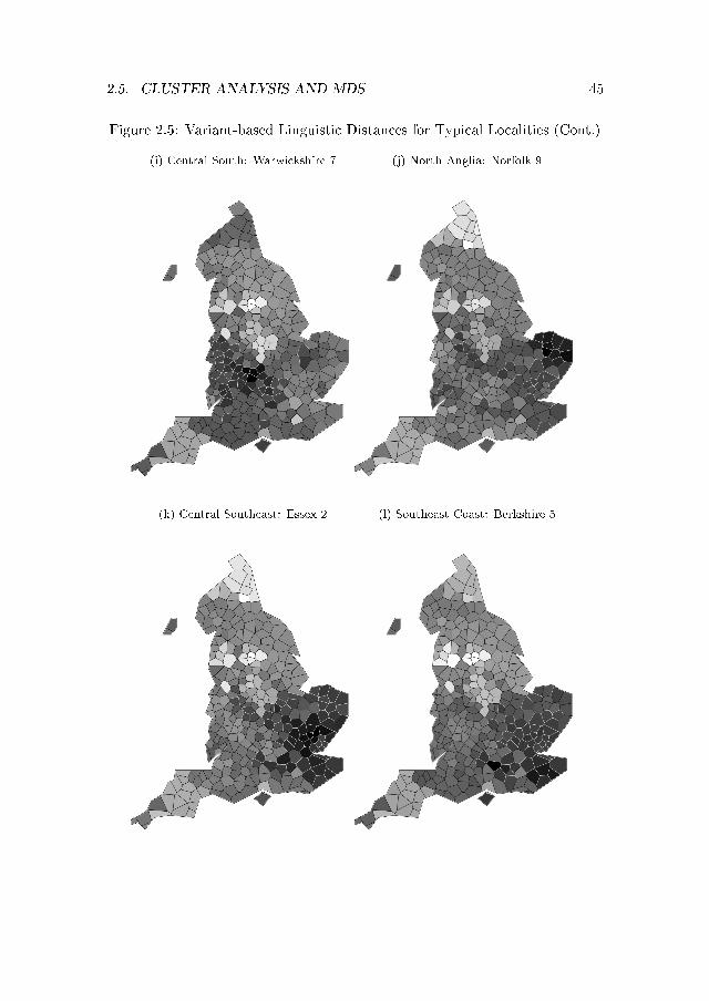
2.5. CLUSTER ANALYSIS AND MDS 45
Figure 2.5: Variant-based Linguistic Distances for Typical Localities (Cont.)
(i) Central South: Warwickshire 7 (j) North Anglia: Norfolk 9
(k) Central Southeast: Essex 2 (l) Southeast Coast: Berkshire 5

46 CHAPTER 2. THE TRADITIONAL ENGLISH DIALECTS
Figure 2.5: Variant-based Linguistic Distances for Typical Localities (Cont.)
(m) Central Southwest: Dorsetshire 3 (n) Devonshire: Devonshire 3
(o) Cornwall: Cornwall 5

2.5. CLUSTER ANALYSIS AND MDS 47
respective regions.) For the Far North, for instance, every locality's vectorof frequencies has a Pearson correlation of 0.86 or higher with the vector ofaverage regional frequencies in the Far North, while the next highest-scoringlocality has a correlation of 0.80. Moreover, in a majority of cases the localitywith the highest correlation with the vector of average regional frequenciesis also the �most typical� locality in the sense of having the lowest averagedistance with all the other localities in the region. Those results reinforcethe impression that the regional clustering is underlain by sets of linguisticcharacteristics in each region to which the localities in the respective regionstend to gravitate.
The dialect regions delineated here are very similar to those found in thedialect map of Trudgill (1999), shown in Figure 2.6, with only a few distinctivedi�erences: the Midlands (in Trudgill's terms, the Central) dialect region ismuch more restricted and is associated with the northern family of dialectsrather than the southern one; the Southeast Coast clusters among the South-eastern dialects rather than the Southwestern ones, and much of Trudgill'sSoutheast clusters into a larger Central Southeastern region that extends upto the Midlands boundary. Moreover, the analysis �nds very little distinctionbetween east and west in the northern dialect regions: parts of Cumberlandconsistently cluster with parts of eastern Yorkshire, and much of Lancashireconsistently clusters with Darbyshire and Nottinghamshire (though not Lin-colnshire).
The delineation presented here also bears a strong resemblance to that de-scribed by Ellis (1889), except that Ellis places the Southeast Coast with theSouthwest and Northamptonshire in the Southeast. It bears similarities toseveral maps presented in some dialectometric studies using lexical and mor-phological variants in the SED but di�ers noticeably from others. It resemblesthe �centers of gravity� described by Händler and Viereck (1997), exhibits amoderate degree of similarity with the clusters identi�ed by Goebl (1997) in acomplete linkage analysis using several distance measures over the same data,and is fairly similar to Thomas's (1997) characterization as well. However, thedelineation is not very similar to that proposed by Goebl and Schiltz (1997)on the basis of localities' number of shared features in that data, even thoughmany of the relatively strong boundaries that they describe appear in Figure2.4; nor is it similar to the dialect division presented by Inoue and Fukushima(1997) on the basis of a multivariate analysis of that data. It remains an openquestion whether or not an exactly analogous approach using lexical and mor-phological data would yield essentially the same demarcation as the presentstudy.

48 CHAPTER 2. THE TRADITIONAL ENGLISH DIALECTS
Figure 2.6: The Traditional Dialect Regions from Trudgill (1999)
Source: The Dialects of England, 2nd Revised Edition, Peter Trudgill, Copyright1999 Blackwell UK. Reproduced by permission.

2.6. MULTIPLE REGRESSION AND BARRIER ANALYSIS 49
2.5.3 Phylogenetic Inference
Applied to the variant-based distance measures, the phylogenies produced bythe Kitsch and Fitch programs strongly support the delineation of dialect re-gions described above, including the major and minor boundaries and the var-ious outliers. The only noticeable deviation is that the Midlands region tendsto expand slightly north to include those localities in Cheshire and Derbyshirethat are closest to Sta�ordshire. In the case of Fitch, the strongest boundaryseparates the Southeast from the rest of England; in the case of Kitsch, itseparates the North and South. Interestingly, and consistent with the modestvariant-based linguistic distance between them, both Received Pronunciationand Western Reserve speech appear as a pair of fairly closely related outliers� within the Southeast in the case of Kitsch, and separate from all the SEDlocalities in the case of Fitch.
2.6 Exploring Dialect Geography: Multiple
Regression and Barrier Analysis
2.6.1 Multiple Regression Analysis
Multiple regression analysis quanti�es the relationships between a variable ofinterest � a dependent variable � and a number of other independent variables,allowing for interaction among the latter.27 For instance, multiple regressioncan be applied to a set of measurements of a group of individuals' weights,heights, waistlines, age, and gender to analyze how their weights vary withtheir other characteristics. (In this example, gender would be represented bya 0 for one gender and a 1 for the other; an independent variable that takesthis form is referred to as a �dummy� variable.)
I use regression analysis to test for a statistically signi�cant relationshipbetween the various measures of linguistic distance between localities and thegeographic distance between them, using the Statistical Package for the SocialSciences (SPSS) for Windows Version 7.5.28 However, by introducing dummyvariables that represent localities' regional a�liations, distance regressions canbe used to explore whether di�erences among localities can be interpreted asbeing more-or-less wholly a matter of geographic separation that has resultedin the gradual accumulation of di�erences over generations, or whether thosedi�erences also vary systematically across the dialect regions identi�ed by clus-ter and phylogenetic analyses.
27See Tabachnick and Fidell (2000), Chapter 5, for an overview of multiple regressionanalysis.
28SPSS is available at http://www.spss.com/.

50 CHAPTER 2. THE TRADITIONAL ENGLISH DIALECTS
2.6.2 Distance Regressions
Table 2.4 shows the results of a regression of the variant-based linguistic dis-tances on the natural logs of geographic distances and on a set of intra- andinterregional dummy variables.29 Each of the 120 dummies takes a value of1.0 only when two localities are from two speci�c regions. For example, thedummy variable �Dummy, Regions 1 and 15� takes a value of 1.0 only whenone locality is in the Far North and the other is in Cornwall. As a result,the parameter that is estimated on this variable is based only on linguisticdistances between localities in those two regions.
Table 2.4: Distance Regressions with Regional Dummy Variables
Variable Value Variable ValueAdjusted R-Square 0.774 Dummy, Regions 3 and 3 0.024*Constant Term 0.35 Dummy, Regions 3 and 4 0.348Distance Coe�cient 0.137 Dummy, Regions 3 and 5 0.126Dummy, Regions 1 and 2 0.385 Dummy, Regions 3 and 6 0.497Dummy, Regions 1 and 3 0.513 Dummy, Regions 3 and 7 0.490Dummy, Regions 1 and 4 0.686 Dummy, Regions 3 and 8 0.678Dummy, Regions 1 and 5 0.534 Dummy, Regions 3 and 9 0.621Dummy, Regions 1 and 6 0.697 Dummy, Regions 3 and 10 0.807Dummy, Regions 1 and 7 0.678 Dummy, Regions 3 and 11 0.760Dummy, Regions 1 and 8 0.603 Dummy, Regions 3 and 12 0.746Dummy, Regions 1 and 9 0.551 Dummy, Regions 3 and 13 0.944Dummy, Regions 1 and 10 0.809 Dummy, Regions 3 and 14 1.182Dummy, Regions 1 and 11 0.802 Dummy, Regions 3 and 15 0.737Dummy, Regions 1 and 12 0.819 Dummy, Regions 4 and 4 0.218Dummy, Regions 1 and 13 0.787 Dummy, Regions 4 and 5 0.178Dummy, Regions 1 and 14 1.250 Dummy, Regions 4 and 6 0.399Dummy, Regions 1 and 15 0.636 Dummy, Regions 4 and 7 0.370Dummy, Regions 2 and 2 0.058* Dummy, Regions 4 and 8 0.583Dummy, Regions 2 and 3 0.107 Dummy, Regions 4 and 9 0.552Dummy, Regions 2 and 4 0.290 Dummy, Regions 4 and 10 0.700Dummy, Regions 2 and 5 0.163 Dummy, Regions 4 and 11 0.682Dummy, Regions 2 and 6 0.383 Dummy, Regions 4 and 12 0.812Dummy, Regions 2 and 7 0.368 Dummy, Regions 4 and 13 0.870Dummy, Regions 2 and 8 0.602 Dummy, Regions 4 and 14 0.995Dummy, Regions 2 and 9 0.589 Dummy, Regions 4 and 15 0.627Dummy, Regions 2 and 10 0.647 Dummy, Regions 5 and 5 0.251Dummy, Regions 2 and 11 0.623 Dummy, Regions 5 and 6 0.469Dummy, Regions 2 and 12 0.753 Dummy, Regions 5 and 7 0.425Dummy, Regions 2 and 13 0.891 Dummy, Regions 5 and 8 0.581Dummy, Regions 2 and 14 1.910 Dummy, Regions 5 and 9 0.557Dummy, Regions 2 and 15 0.685 Dummy, Regions 5 and 10 0.788
Continued on Next Page
29That approach is consistent with the observation that increasing distance tends to havea decreasing incremental in�uence on linguistic di�erences.

2.6. MULTIPLE REGRESSION AND BARRIER ANALYSIS 51
Table 2.4 : Distance Regressions with Regional Dummy Variables (Continued)
Variable Value Variable ValueDummy, Regions 5 and 11 0.698 Dummy, Regions 8 and 14 0.676Dummy, Regions 5 and 12 0.885 Dummy, Regions 8 and 15 0.201Dummy, Regions 5 and 13 0.838 Dummy, Regions 9 and 9 0.175Dummy, Regions 5 and 14 1.820 Dummy, Regions 9 and 10 0.420Dummy, Regions 5 and 15 0.567 Dummy, Regions 9 and 11 0.440Dummy, Regions 6 and 6 0.125 Dummy, Regions 9 and 12 0.467Dummy, Regions 6 and 7 0.193 Dummy, Regions 9 and 13 0.426Dummy, Regions 6 and 8 0.622 Dummy, Regions 9 and 14 0.600Dummy, Regions 6 and 9 0.453 Dummy, Regions 9 and 15 0.148Dummy, Regions 6 and 10 0.486 Dummy, Regions 10 and 10 0.105Dummy, Regions 6 and 11 0.469 Dummy, Regions 10 and 11 0.161Dummy, Regions 6 and 12 0.647 Dummy, Regions 10 and 12 0.329Dummy, Regions 6 and 13 0.912 Dummy, Regions 10 and 13 0.610Dummy, Regions 6 and 14 1.930 Dummy, Regions 10 and 14 0.946Dummy, Regions 6 and 15 0.717 Dummy, Regions 10 and 15 0.487Dummy, Regions 7 and 7 0.041* Dummy, Regions 11 and 11 0.105Dummy, Regions 7 and 8 0.568 Dummy, Regions 11 and 12 0.289Dummy, Regions 7 and 9 0.456 Dummy, Regions 11 and 13 0.700Dummy, Regions 7 and 10 0.404 Dummy, Regions 11 and 14 0.935Dummy, Regions 7 and 11 0.353 Dummy, Regions 11 and 15 0.450Dummy, Regions 7 and 12 0.538 Dummy, Regions 12 and 12 0.920Dummy, Regions 7 and 13 0.854 Dummy, Regions 12 and 13 0.621Dummy, Regions 7 and 14 0.995 Dummy, Regions 12 and 14 0.830Dummy, Regions 7 and 15 0.591 Dummy, Regions 12 and 15 0.365Dummy, Regions 8 and 8 0.262 Dummy, Regions 13 and 13 0.780Dummy, Regions 8 and 9 0.268 Dummy, Regions 13 and 14 0.272Dummy, Regions 8 and 10 0.446 Dummy, Regions 13 and 15 0.000Dummy, Regions 8 and 11 0.494 Dummy, Regions 14 and 14 0.142Dummy, Regions 8 and 12 0.442 Dummy, Regions 14 and 15 0.180Dummy, Regions 8 and 13 0.349 Dummy, Regions 15 and 15 0.048*
* - Not signi�cant at the 0.99 level. . .
According to the adjusted R-square of the variant-based regression, ge-ographic distance and regional di�erences account for about 77 percent ofthe variation in measured linguistic distances. (Excluding the dummies, ge-ographic distance alone accounts for about 50 percent.) All but four of theregional dummy variables have p-values of 0.01 or less � an unusually strongresult in any kind of cross-section regression, and pointing to speakers' re-gional a�liations as an important source of their linguistic (dis)similarities.The value of the parameter for the geographic distance variable indicates thatignoring regional a�liation � itself, however, partly a function of geographicdistance � 100 miles of distance between two localities increases their linguis-tic distance by about 0.63 (0.137 times 4.605, the natural log of 100), and the

52 CHAPTER 2. THE TRADITIONAL ENGLISH DIALECTS
average geographic distance of 129 miles should result in a linguistic distanceof about 0.67, roughly 54 percent of the average linguistic distance.
The results of the feature-based regression (not shown) are quite similar:the adjusted R-square of the regression indicates that geographic distance andregional di�erences account for about 80 percent of the variation in feature-based linguistic distances; all but six of the regional dummy variables are highlysigni�cant; geographic distance parameter indicates that ignoring regional af-�liation, the average geographic distance should result in a linguistic distanceof about 0.68, about 62 percent of the average distance.
When dummy variables are included in a regression, one of them is left out,and the constant term is, in e�ect, the parameter for that dummy. (The propervalues for the other dummy parameters therefore also include the constantterm.) In this analysis, the constant term applies to localities within theRegion 1, the Far North, indicating that all else being equal, hypotheticalspeakers living in the same location in Region 1, the Far North, would have avariant-based distance of about 0.035 and an average feature-based linguisticdistance of 0.233 � again illustrating the fact that the smallest feature-baseddistances tend to be larger than the smallest variant-based distances. For eachdistance measure, the value of the parameter for �Dummy, Regions 8 and 8�indicates that localities in the West Midlands typically are considerably moredistinct from each other than those in the Far North are from each other.30
The interregional dummy variables take similar interpretations, except thatby construction they incorporate into the value of the dummy parameter thee�ect of the average distance between locations in two separate regions. Thus,for instance, the values of �Dummy, Regions 1 and 14� (1.025) and �Dummy,Regions 1 and 15� (0.636) in Table 2.4 indicate that the variant-based distancebetween two randomly chosen localities from the Far North and Devonshireis likely to be considerably larger than that between two localities from theFar North and Cornwall, despite the fact that the Far North is very nearlythe same distance from Devonshire and Cornwall. However, the correspondingvalues for the feature-based regression are noticeably smaller, re�ecting thefact that the feature-based linguistic distances are not as widely dispersed asthe variant-based linguistic distances.
The Pearson correlation between feature-based and variant-based dummiesacross equivalent regions is quite high � 0.82 � despite the fact that values forindividual dummies are frequently very di�erent. That strong correlation �
30The negative value of the parameter for �Dummy, Regions 5 and 5� in the variant-basedregression has no realistic interpretation, but it indicates that localities in Lincolnshire aremuch more similar to each other than is typical in most regions of England. The insigni�-cant values for four intraregional dummies imply that the e�ect of geographic distance onintraregional linguistic di�erences in those regions cannot be distinguished from its e�ect onsuch di�erences in the Far North.

2.6. MULTIPLE REGRESSION AND BARRIER ANALYSIS 53
nearly as strong as the correlation between variant-based and feature-basedlinguistic distances � provides another indication that the regional variationsuncovered in this analysis are quite robust to di�erent characterizations of thephonetic data and likely re�ect real patterns of dialect variation.
Table 2.5 illustrates the importance of regional speech di�erences, showingthe percentage di�erence between the average predicted variant-based linguis-tic distances between localities in di�erent regions, with and without regionaldummies. Positive values indicate that localities in the relevant regions havegreater-than-average speech di�erences, given their geographic separation; neg-ative values point to smaller linguistic di�erences. For example, one of thelargest values in Table 2.5, 24.9 for interregional di�erences between Sta�ord-shire and the bordering West Midlands, indicates that the dialect boundarybetween the two regions is a particularly signi�cant one. Conversely, the quitenegative values between North Anglia, the Central Southeast, and the South-east Coast point to relatively uniform speech across those three regions. Gen-erally speaking, the largest values in the table apply to di�erences betweendialect regions in the Midlands and Upper Southwest, suggesting that there isa broad central region of England of particularly great dialect diversity, per-haps because the conditions for interaction and in�uence among speakers isgreater in a wide transition zone between the North, Southeast, and South-west. Note also that the highest values among intraregional dummies are forSta�ordshire, the West Midlands, and the South Central region, all part of thelarge transition zone in the center of England; but the East Midlands dummytakes a very low value, indicating that it, like its eastern neighbor Lincolnshire,is a much more uniform region linguistically than most of the regions to itswest. The variant-based and feature-based values are generally similar, with aPearson correlation of 0.69.
The fact that the intraregional dummy variables include a distance compo-nent complicates the interpretation of their values and that of the geographicdistance term as well. Put simply, the e�ect of geographic distance on speechdi�erences between regions is highly variable. Other non-geographic in�uencesalso a�ect linguistic di�erences over long distances; they are not quite as im-portant as geographic distance alone, on average, but between some regionsthey can be at least as important, either enhancing or o�setting the e�ect ofgeographic distance on speech di�erences.

54 CHAPTER 2. THE TRADITIONAL ENGLISH DIALECTS
Table
2.5:
PercentageDi�erence
betweenCalculatedDistanceScores
Based
onVariant-based
RegressionResults
withandwithout
RegionalDum
myVariables
Region
(1)
(2)
(3)
(4)
(5)
(6)
(7)
(8)
(9)(10)(11)(12)(13)(14)(15)
(1)FarNorth
-30.3
-4.0
8.3
8.7
-6.4
3.3
-0.3
-7.7
-12.4
5.3
2.7
1.1
-0.4
12.3
-13.4
(2)Upper
Northwest
-4.0
-44.7
-26.8
-16.5
-29.7
-14.4
-17.6
-3.6
-5.8
-1.1
-5.2
0.3
9.8
19.6
-9.0
(3)Cumbria-NorthYorkshire
8.3
-26.8
-15.7
-7.3
-34.8
-3.2
-8.5
4-3.3
7.9
3.3
-0.3
14.2
27.1
-4.8
(4)Low
erNorthwest
8.7
-16.5
-7.3
-15.1
-26.0
0.8
-9.5
4.0
-1.6
5.8
3.5
8.9
14.8
19.0
-9.8
(5)Lincolnshire
-6.4
-29.7
-34.8
-26-64.9
-0.9
1.5
-1.1
0.8
29.5
12.8
17.8
11.9
22.0
-15.1
(6)Sta�ordshire
3.3
-14.4
-3.2
0.8
-0.9
-2.1
-16.4
24.9
1.1
-8.4
-8.1
2.5
27
32.2
-1.4
(7)East
Midlands
-0.3
-17.6
-8.5
-9.5
1.5
-16.4
-23.8
9.0
9.3
-7.7
-10.0
-1.3
23.1
22.9
-10.9
(8)WestMidlands
-7.7
-3.6
4.0
4.0
-1.1
24.9
9.0
-2.0
-15.5
-14.7
-7.7
-11.4
-11.1
10.1
-33.4
(9)CentralSouth
-12.4
-5.8
-3.3
-1.6
0.8
1.1
9.3
-15.5
-4.7
-10.2
1.2
1.6
-2.1
-0.9
-38.4
(10)East
Anglia
5.3
-1.1
7.9
5.8
29.5
-8.4
-7.7
-14.7
-10.2
-15.2
-24.5
-19.1
-3.8
12.3
-20.4
(11)CentralSoutheast
2.7
-5.2
3.3
3.5
12.8
-8.1
-10.0
-7.7
1.2
-24.5
-20.3
-13.7
10.1
16.3
-20.8
(12)Southeast
Coast
1.1
0.3
-0.3
8.9
17.8
2.5
-1.3
-11.4
1.6
-19.1
-13.7
-28.3
11.3
13.3
-24.6
(13)CentralSouthwest
-0.4
9.8
14.2
14.8
11.9
27.0
23.1
-11.1
-2.1
-3.8
10.1
11.3
-25.8
-17.9
-46.7
(14)Devonshire
12.3
19.6
27.1
19.0
22.0
32.2
22.9
10.1
-0.9
12.3
16.3
13.3
-17.9
-50.3
-25.0
(15)Cornwall
-13.4
-9.0
-4.8
-9.8
-15.1
-1.4
-10.9
-33.4
-38.4
-20.4
-20.8
-24.6
-46.7
-25.0
-34.4

2.6. MULTIPLE REGRESSION AND BARRIER ANALYSIS 55
The regression results yield several important insights. The highly signi�-cant geographic distance coe�cients suggest that regional dialect diversity isclosely tied to geographic separation and that such diversity is largely con-tinuous. Distance alone accounts for at least half of phonetic variation inthe traditional English dialects. However, di�erences in the magnitudes ofthe intraregional dummy variables point to regions of relative uniformity aswell as regions of much greater diversity, controlling for geographic distance.Moreover, the highly statistically signi�cant dummy parameters indicate thatsystematic di�erences between regional speech forms account for roughly aquarter of the variation in the dialects.
2.6.3 Variant-Area Regressions
A regression of the number of variants in each region on the number of localitiesfurther reinforces the sense of varying degrees of regional uniformity. Biologistshave long noted a regular correspondence between the (log of the) number ofspecies that inhabit a geographic region and (the log of) its size � the species-area relationship. Consistent with the view that speech variants inhabit aspeech region and are subject to mutation and selection pressures analogousto those that a�ect species in the biosphere, a similar pattern tends to obtainbetween the number of speech variants in use and the number of speakers. Inthe present data set, there is a high degree of correlation between the numberof variants and the number of localities in the 15 regions delineated by clusterand phylogenetic analysis; a log-log regression of the number of variants on thenumber of speakers suggests that an additional interview in another locality ina region will typically increase the number of variants found in the region byabout 1.3, and that such a relationship accounts for about two-thirds of thevariation in the number of variants by region.
However, the errors or residuals in the variant-area regression provide usefulinformation about the relative uniformity of speech in di�erent regions. Thoseerrors are particularly positive in Linconshire, Cumbria-North Yorkshire, andthe Central Southeast, while the most negative errors are for Sta�ordshire,the Central South region, and the Southeast Coast. Those errors indicatethat the former group of regions � which are also regions in which linguisticdistances are relatively small compared with geographic ones � tend to havelower diversity in terms of the number of variants, while the latter group �which also tend to have greater linguistic diversity over a given geographicdistance � tend to have greater diversity in terms of the number of variants.

56 CHAPTER 2. THE TRADITIONAL ENGLISH DIALECTS
2.6.4 Barrier Analysis
The importance of geography in determining the distribution of speech formscan be further analyzed by examining the distribution of residuals or errorsin regressions of linguistic distance on geographic distance: a series of largepositive errors generally indicates an important dialect boundary that marksa relatively large number of linguistic changes over a short distance, whereasa series of large negative errors probably indicates unusually uniform speechover a relatively broad area. Monmonier (1973) developed a maximum di�er-ence algorithm that analyzes distance measures to map important boundaries.An illuminating example of its use by Manni and Barrai (2001) tests the asso-ciations between dialect di�erences, gene frequencies, and the distribution ofsurnames in the Italian province of Ferrara. Applied to English dialect data,Monmonier's algorithm may complement regression analysis in identifying im-portant speech boundaries. The algorithm is implemented using the BarrierVersion 2.2 software package developed by Manni, Guérard, and Heyer.31
Applied to matrices of feature-based and variant-based linguistic distances,Monmonier's algorithm produces broadly similar results that are, in each case,largely consistent with the regional classi�cation developed above. (Applyingthe algorithm to residuals of a regression of variant-based or feature-based dis-tances on geographic distances tends to yield similar patterns.) The algorithmidenti�es many of the same regional boundaries as do the cluster and phylo-genetic analyses, including those between the Southeast and Southwest, theUpper Southwest and the Central Midlands, the Far North and Upper North,and the subregions of the Southeast, Upper Southwest, and Lower Southwest.The algorithm also identi�es several other barriers within regions: using ei-ther set of distance measures, it isolates areas of south Lancashire, Cheshire,and Derbyshire as distinctive subregions; and using one measure or the other,it isolates West Yorkshire, Devonshire, Somerset, or Essex. However, the al-gorithm tends not to �nd clear boundaries along the eastern English coast,between Yorkshire and Lincolnshire, Lincolnshire and the East Midlands, orEast Midlands and the Southeast.
In addition, however, roughly half of the boundaries the algorithm identi�esisolated individual localities that are particularly distinct from their neighbors.A few of those lie well away from any of the others, such as Cumberland1 and Essex 7, and a few are in Hampshire on the boundary between theLower Southwest and the Southeast Coast. However, pointing yet again to theregion's unusual linguistic diversity, the great majority of distinctive localities
31Barrier Version 2.2 is freely available online at http://www.mnhn.fr/mnhn/
ecoanthropologie/software/barrier.html.

2.7. PRINCIPAL COMPONENT ANALYSIS 57
are in or near the Upper Southwest, including Shropshire 2 and 5, severallocalities in Monmouth, Gloucestershire 4, Worcestershire 1 and 7, Oxfordshire2 and 3, Buckingham 6, and Hertfordshire 3.
2.7 Uncovering Linguistic Structure: Principal
Component Analysis
Like cluster analysis and MDS, principal component analysis (PCA) reducesthe number of dimensions in a data set, but it does so by �nding groups ofstrongly correlated variables that are uncorrelated with the rest of the vari-ables, and reducing them to a single �latent� variable � called a principal com-ponent or PC � that is essentially a linear combination of the correlated vari-ables.32 In e�ect, PCA clusters groups of variables (in this case, feature valuesor variant frequencies) in a manner somewhat analogous to how cluster anal-ysis distinguishes groups of observations (in this case, localities). PCA maythus allow a researcher to summarize the patterns of relationship among thevariables as a smaller number of uncorrelated variables that contain most ofthe information in the data set.
Applied to a data set of linguistic features, PCA may isolate groups ofvariants or features that tend to occur together and that, with any luck, havea structural linguistic interpretation. Component scores, which measure thestrength of a particular principal component in the data for each locality, mayreveal associations between those linguistic structures and speci�c regions. Inshort, a properly performed and interpreted PCA may provide a relativelyobjective way of de�ning dialects and dialect regions. I use the Statistical
32Tabachnick and Fidell (2000), Chapter 13, provides an introduction to principal com-ponent analysis, as does Bartholomew et al. (2002), Chapter 5. Several recent studies haveapplied principal component analysis or the closely related factor analysis to linguistic data,including Labov et al.'s (2006) and Clopper and Paolillo's (2006) analyses of acoustic fea-tures of North American English, Nerbonne's (forthcoming) analyses of variation in Middleand Southern Atlantic American English, and Shackleton's (2005) examination of usage dif-ferences among speakers of various English and American dialects. As noted by Nerbonne,an argument can be made that principal component analysis, which is essentially an ex-ploratory technique, is less preferable to use for the present analysis than factor analysis,which is more appropriate when the aim of the analysis is to uncover underlying structures� or �latent variables� � that are manifested in the variables under analysis. However, factoranalysis requires a matrix of variables in which none of the rows are linear combinationsof the others, which for the variant-based analysis requires that localities' frequencies ofthe various pronunciations of a given set of words cannot sum to 100 percent. Moreover,principal component analysis and factor analysis typically yield very similar results, so theadvantages of being able to examine all pronunciations in the data would appear to outweighthe advantage of being able to rigorously uncover latent variables.

58 CHAPTER 2. THE TRADITIONAL ENGLISH DIALECTS
Package for the Social Sciences (SPSS) for Windows Version 7.5 for the variant-based analysis and SAS/STAT 9.1 for the feature-based analysis.33
PCA uncovers sets of variables whose values are strongly positively or neg-atively correlated � that is, groups of variants that tend to occur together orthat tend to occur separately. (Variables that always occur separately are notindependent; mathematically speaking, independence � or orthogonality � im-plies that there is no pattern of co-occurrence at all. In visual terms, negativecorrelation places variants at opposite poles of a line, such as north and south,while independence places them at ninety degrees to each other on a perpen-dicular line � that is, north and east.) PCs therefore typically have two poles:one pole will have large positive values, or loadings, for a group of variablesthat tend to be found together; the other will have large negative values foranother group of variables that are also found together but never with the �rstgroup.34
In the standard approach, each PC is uncorrelated with � or orthogonalto � all the others. The �rst PC �extracts� or accounts for the maximumpossible variance from the data set that can be accounted for by a single linearcombination of variables; the second extracts the maximum possible amountof the remaining variance, and so on. Each variable is assigned a score in eachPC, but will typically take low values in all but one or at most a few PCs. Foreach PC a component score for each observation can be calculated as the sumof the products of each variable's value in the observation and the variable'sscore in the PC. A given observation may have high component scores forseveral quite di�erent PCs.
Several variations on the standard PCA approach allow for the adjustmentof PCs in ways that simplify them, generally by placing more emphasis onthe highest-scoring variants (in technical terms, by �rotating� them to increasethe loading on those variables). Orthogonal rotations leave the PCs uncor-related, whereas non-orthogonal rotations allow for some correlation betweenPCs. In the present study, orthogonal rotation typically yields more clearlyinterpretable sets of variables than does standard PCA � especially when ap-plied to variants rather than to features � and the groups of variables thusidenti�ed appear also to be used by localities in more sharply de�ned regions.For the data used in this study, however, non-orthogonal PCA produces PCsthat are very largely uncorrelated, so that non-orthogonal rotation appears tobe unnecessary.
PCA yields a large number of PCs, raising the issue of how many to inter-pret as yielding useful information. Although there is no hard and fast rule
33SAS/STAT is available at http://www.sas.com/technologies/analytics/statistics/stat/index.html.
34As a rule of thumb, researchers take into consideration only variables with laodings of0.32 and larger in absolute value as part of a PC. See Costello and Osborne (2005), p. 4.

2.7. PRINCIPAL COMPONENT ANALYSIS 59
in this regard, the most widely recommended approach is called the �scree�test, which recommends retaining PCs that account for the greatest amount ofvariation up to the point at which the explained variation drops precipitouslyfrom one PC to the next, and disregarding PCs below the �break.�35 Apply-ing PCA to the feature-based and variant-based data yields obvious breaks,but several of the PCs beyond the breaks are easily interpretable in linguisticterms and have component scores that link them to geographically coherentregions that are similar, in many cases, to the regions delineated by the clusteranalyses, suggesting that in some cases the scree test may be safely ignored.
2.7.1 Feature-Based Results
Because it allows for continuous variation in articulation, the feature-basedPC analysis yields PCs whose values vary continuously as a function of articu-lation. Only a handful of unrotated PCs yield clear, easily interpreted resultsin the feature-based approach. Consider the �rst unrotated PC, whose PCscores are presented in Table 2.6 and whose component scores are illustratedin Figure 2.7a, and which captures about 12 percent of total variation in thedata. The �rst PC clearly distinguishes southern � and particularly Southwest-ern � English features from northern ones, with more central regions yieldingintermediate component scores. The features with the highest loadings gener-ally involve the raising or lengthening of some short vowels, the backing androunding of /a/ after /w/, and the lowering, backing, and unrounding of /u/� all general southern English innovations. Other features associated with theSouthwest also take relatively large loadings in the PC, including manner ofrhoticity and fricative voicing. Southeastern [l]-vocalization also has a rela-tively strong loading, and another set of large loadings obtains for degrees ofheight, backing, and rounding in many of the diphthongized Middle Englishlong vowels. (Recall that the values describing the second element of a diph-thong are converted to di�erences between the second element and the �rst.)These values have a straightforward interpretation: upgliding variants like [6i∼ Oi] in night or [æi ∼ ai] in gate will tend to yield relatively large positiveloadings, while long or ingliding variants like [i:] in night or [ia] in gate willyield large negative loadings.
35The recommendation is generally phrased in terms of highest eigenvalues rather thanhighest explanatory value. The widely recommended practice of retaining PCs with eigen-values greater than 1.0 is among the least accurate of methods. See Costello and Osborne(2005).

60 CHAPTER 2. THE TRADITIONAL ENGLISH DIALECTS
Table2.6:
Loadings:
First
Feature-basedUnrotated
Principal
Com
ponent
First
Vow
elSecondVow
elRhotic
Consonant
Height
Back-Round-Length
HeightBack-Round-Length
Place
Manner
Frica-
Aspi-
GlottalVelar
Other
Word
ing
ing
ing
ing
tive
rate
Stop
Short
Apple
0.394
−−
0.113
0.053
−−
−−
−−
−0.276−0.702
−Catch
0.531
−−
−−
−−
−−
−−
−−
−−
Ask
0.266
0.230
−0.759
−−
−−
−−
−−
−−
−Father
−0.057
0.261
−0.620−0.145−0.176
−0.010−0.063
0.593
0.438
−−
−−
Wasp
0.181
0.690
0.686
0.119
−−
−−
−−
−−
−−
−Water
0.643
0.780
0.758
0.818−0.042−0.163−0.147
−0.158
0.202
0.511
0.410
−0.110
−−
Aunt
0.087
0.140−0.143
0.695
−−
−−
−−
−−
0.072
−−
Yellow(1)
0.318
−0.158−0.146
−−
−−
−−
−−
−−
−0.498
−Fox
−0.150
0.067−0.091
0.056
−−
−−
−−
0.481
−−
−−
Yolk
−0.154
0.060−0.189
−0.099
0.393
0.117
0.402
0.096
−−
−−
−0.153
−Cross
0.470
0.096−0.086
0.768
−−
−−
0.188
0.386
−−
−−
−Women
0.081
−−
−−
−−
−−
−−
−−
−−
Colt
0.432
0.343
0.222
0.400−0.339−0.261−0.222
−−
−−
−−0.066
−−
Sun
−0.680
0.481−0.151
−−
−−
−−
−0.477
−−
−−
Butter
−0.711
0.657−0.750
−−
−−
−0.075
0.478
0.293
−0.199
−−
ShortRhotic
Farm
−0.003
0.334
−−0.437
−−
−−
−0.032
0.579
0.395
−−
−−
Forty
0.147
−0.360−0.364
0.068−0.158−0.074−0.115
−0.042−0.002
0.593
0.430
−−0.257
−0.615
Hurt
0.240
−0.421−0.520
−0.103
−−
−−
0.090
0.595
0.694−0.085
0.102
−−
Continued
onNextPage

2.7. PRINCIPAL COMPONENT ANALYSIS 61
Table2.6:Loadings:
First
Feature-BasedUnrotatedPrincipalComponent(Continued)
First
Vow
elSecondVow
elRhotic
Consonant
Height
Back-Round-Length
HeightBack-Round-Length
Place
Manner
Frica-
Aspi-
GlottalVelar
Other
Word
ing
ing
ing
ing
tive
rate
Stop
Long
Gate
−0.404
0.273
−−0.087
0.479
0.207
−−0.043
−−
−−
−−
−Potato
(1)
−0.099
0.176
−−0.331
0.219−0.150
−0.058
−−
−−
−−
−Meat
0.034
−0.053
−0.188
0.177−0.373
−0.119
−−
−−
−0.043
−−
Peas
0.158
−0.012
−0.199
0.098−0.268
−0.137
−−
−−
−−
−Cheese
0.163
−0.034
−0.096−0.097−0.107
−0.085
−−
−−
−−
−Wheel
0.195
−0.022
−0.021−0.459
0.508
0.335
−0.410
−−
−−0.263
−−0.758
−White
0.270
0.498
0.460
−0.121−0.200−0.530−0.451
0.134
−−
−−0.268
0.071
−−
Blind
−0.530
0.353
0.361
0.023
0.469−0.414−0.390
0.094
−−
−−
−−
−Night
−0.628
0.510
0.435
−0.451
0.538−0.392−0.407
−0.205
−−
−−
−−
−Both
−0.351
0.740
0.444
0.371
0.587−0.156
0.309
−0.009
−−
0.420
−−
−−
Comb
0.097
0.441
0.100
0.178
0.383−0.301
0.207
−0.227
−−
−−
−−
−Loaf
−0.366
0.581
0.098
0.201
0.582−0.076
0.333
0.140
−−
0.248
−−
−−
None
−0.403
0.507−0.060
0.212
0.646−0.140
0.286
0.013
−−
−−
−−
−Cold
0.303
0.342
0.215
−0.459
0.114−0.139
0.087
0.120
−−
−−
−0.307
−Nose
−0.461
0.497−0.179
0.224
0.554
0.211
0.604
0.049
−−
−−
−−
−Potato
(2)
−0.290
0.166
0.042
0.330
−−
−−
0.392
0.392
0.438
−0.176
−−
Moon
0.181
0.333
0.455
0.369
0.217−0.255−0.089
0.072
−−
−−
−−
−Wool
0.005
−0.157
0.060
−0.047−0.181−0.282−0.187
−0.230
−−
−−
−−0.427−0.242
Roof
−0.059
0.313
0.372
0.166
0.250−0.345−0.153
−0.105
0.202
0.461
−−
−−
−House
−0.368
−0.464−0.469
−0.475
0.349
0.472
0.328
−0.162
−−
0.166−0.032
−−
−LongRhotic
Mare
−0.505
−0.594
−0.028
0.422
0.345−0.213
−0.199
0.193
0.494
−−
−−
−Hear
0.327
−0.345
−−0.120−0.313
0.208−0.236
0.041
0.118
0.528
−−0.049
−−
−Fire
0.390
0.528
0.407
−0.023−0.306−0.534−0.407
0.062
0.073
0.566
0.503
−−
−−
More
0.090
0.734
0.616
0.128−0.166−0.553−0.458
−0.249
0.117
0.550
−−
−−
−Door
−0.191
0.529
0.452
0.291−0.259−0.635−0.560
−0.344
0.000
0.508
−−
−−
−Hour
−0.429
−0.342−0.390
−0.240
0.439
0.359
0.366
0.023
0.138
0.502
−−
−−
−Continued
onNextPage

62 CHAPTER 2. THE TRADITIONAL ENGLISH DIALECTS
Table2.6:Loadings:
First
Feature-BasedUnrotatedPrincipalComponent(Continued)
First
Vow
elSecondVow
elRhotic
Consonant
Height
Back-Round-Length
HeightBack-Round-Length
Place
Manner
Frica-
Aspi-
GlottalVelar
Other
Word
ing
ing
ing
ing
tive
rate
Stop
Diphthong
Daisy
−0.408
−0.096
−−0.467
0.609
0.092
−0.080
−−
−−
−−
−Eight
−0.296
−0.049
−0.078
0.137
0.002−0.070
−0.081
−−
−−
0.05
−−
Voice
−0.141
0.016
0.040
−0.005
−−
−−
−−
−−
−−
0.024
Straw
−0.373
0.435
0.383
0.344
0.413−0.286−0.158
−0.157
0.196
0.251
−−
−−
0.110
Thaw
0.366
0.564
0.403
0.584−0.544−0.346−0.418
−0.004
0.183
−0.374
−−
−−
Daughter
0.374
0.113
0.122
0.843−0.858−0.168−0.450
−0.155
0.069
0.522
0.314
−0.165
−−
Dew
0.171
0.379
0.459
0.365−0.212−0.432−0.440
−0.224
−−
−−
−−
0.280
Tuesday
0.125
0.386
0.478
0.429−0.177−0.461
−−0.295
−−
−−
−−
0.266
Snow
0.118
0.284
0.060
−0.417
0.372−0.065
0.245
0.052
−−
0.279
−−
−−
Yellow(2)
−0.055
0.144
0.159
0.036
0.193−0.134
−−
0.496
0.514
−−
−−
−DiphthongRhotic
Hair
−0.046
−0.162−0.111
−0.247
0.228
0.207−0.249
−0.085
0.321
0.484
−0.029
−−
−Other
Very
−−
−−
−−
−−
−−
−−
−−
0.065
Kitten
−−
−−
−−
−−
−−
0.266
−0.422
−−
Note:�Other�consonants
are:voicingof[t]in
forty,loss
of[w]in
wool,[w]for[v]in
voiceandvery,intrusive[r]in
straw,and
palatalizationin
dewandTuesday.Yellow(1)andYellow(2)referto
the�rstandsecondvocalicsegments,respectively,andPotato
(1)
andPotato
(2)referto
thesecondandthirdvocalicsegments.

2.7. PRINCIPAL COMPONENT ANALYSIS 63
The �rst PC is thus capturing the contrast between southern upglides andnorthern inglides or downglides, and is translating longer glides into larger PCscores. In this sense, the PC summarizes the historical developments of a groupof Middle English long vowels. Nevertheless, it captures amalgams of southernand northern speech patterns that do not represent the speech patterns of anyparticular locality: many of the Southwestern features to which it assigns largepositive loadings � fricative voicing and rhoticity in particular � are not foundin the Southeast, and upgliding is generally muted in the Southwest.
In contrast to the �rst PC, the second, which accounts for about 10 per-cent of the variation and whose component scores appear in Figure 2.7b, clearlydistinguishes the Southeast and Central Midlands regions from both the South-west and the North, assigning negative scores to the former and its strongestnegative scores to localities nearest London � precisely those localities in whichupglides tend to be most extended. While the PC does a good job of locatingupgliding in the appropriate regions, however, it assigns positive loadings notonly to ingliding features in the North but also to rhotic and fricative featuresfound in the Southwest. In this case, in e�ect, negative loadings identify agroup of dialect regions by the presence of upglides and by the absence ofSouthwestern and Northern features.
The third unrotated PC, accounting for 5 percent of the variation andshown in Figure 2.7c, isolates the Far North by its place of articulation ofrhotics, by the preservation of /h/ and /hw/, and by certain ingliding features.The fourth PC (shown in Figure 2.7d) rather indistinctly isolates the SevernValley by its negative scores, the �fth the Far North once again by certaininglides, and the sixth, localities in the Lower Northwest and Sta�ordshirewith strongly rounded upglides in the mid-back Middle English long vowels.
Varimax rotation reallocates the variance captured in the unrotated PCinto rotated ones, increasing each PC's loadings on somewhat smaller groupsof variables and thus sharpening the focus and regional concentration of eachPC. As shown in Table 2.7 and Figure 2.8a, the features that yield large positiveloadings for the �rst varimax PC and the high-scoring localities are much moredistinctively Southeastern rather than generally southern: the short voweldevelopments and upgliding diphthongization tend to receive higher positiveloadings, but rhoticity and fricative voicing do not. The PC thus distinguishesSoutheastern upgliding from northern ingliding much more clearly than doesthe �rst unrotated PC. Similarly, the second varimax PC � shown in Figure2.8b � much more clearly distinguishes manner of rhoticity and, secondarily,fricative voicing as the distinctive sets of generally Southwestern features, whilethe third PC (Figure 2.8c) isolates fricative voicing as the distinctively LowerSouthwestern features.

64 CHAPTER 2. THE TRADITIONAL ENGLISH DIALECTS
Figure 2.7: Feature-based Unrotated Principal Components
(a) First Component (b) Second Component
(c) Third Component (d) Fourth Component
Note: Darker (lighter) shading indicates larger positive (negative) scores.
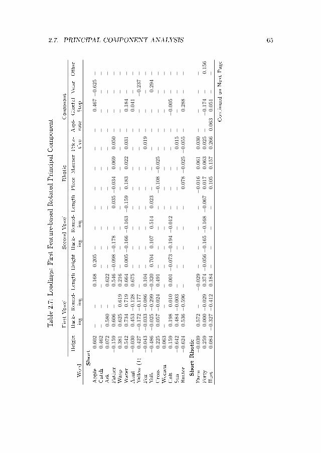
2.7. PRINCIPAL COMPONENT ANALYSIS 65
Table2.7:
Loadings:
First
Feature-basedRotated
Principal
Com
ponent
First
Vow
elSecondVow
elRhotic
Consonant
Height
Back-Round-Length
HeightBack-Round-Length
Place
Manner
Frica-
Aspi-
GlottalVelar
Other
Word
ing
ing
ing
ing
tive
rate
Stop
Short
Apple
0.602
−−
0.168
0.205
−−
−−
−−
−0.467−0.625
−Catch
0.462
−−
−−
−−
−−
−−
−−
−−
Ask
0.072
0.580
−0.622
−−
−−
−−
−−
−−
−Father
−0.159
0.606
−0.546−0.098−0.178
−0.035−0.034
0.069
0.050
−−
−−
Wasp
0.381
0.625
0.619
0.216
−−
−−
−−
−−
−−
−Water
0.542
0.734
0.719
0.664
0.005−0.166−0.163
−0.159
0.183
0.022
0.031
−0.184
−−
Aunt
−0.030
0.453−0.128
0.675
−−
−−
−−
−−
0.041
−−
Yellow(1)
0.427
−0.172−0.177
−−
−−
−−
−−
−−
−0.237
−Fox
−0.043
−0.033−0.086
0.104
−−
−−
−−
0.019
−−
−−
Yolk
−0.486
−0.025−0.299
−0.320
0.704
0.107
0.514
0.023
−−
−−
−0.294
−Cross
0.225
0.057−0.024
0.491
−−
−−
−0.108
−0.025
−−
−−
−Women
0.063
−−
−−
−−
−−
−−
−−
−−
Colt
0.159
0.198
0.010
0.001−0.073−0.194−0.012
−−
−−
−−0.005
−−
Sun
−0.642
0.484−0.003
−−
−−
−−
−0.015
−−
−−
Butter
−0.624
0.536−0.596
−−
−−
−0.078
−0.025
−0.055
−0.288
−−
ShortRhotic
Farm
−0.039
0.572
−−0.029
−−
−−
−0.016
0.061
0.030
−−
−−
Forty
0.259
0.000−0.029
0.374−0.056−0.165−0.168
−0.067
0.017
0.063
0.025
−−0.174
−0.156
Hurt
0.084
−0.327−0.412
0.184
−−
−−
0.105
0.157
0.266
0.063
0.051
−−
Continued
onNextPage

66 CHAPTER 2. THE TRADITIONAL ENGLISH DIALECTS
Table2.7:Loadings:
First
Feature-BasedRotatedPrincipalComponent(Continued)
First
Vow
elSecondVow
elRhotic
Consonant
Height
Back-Round-Length
HeightBack-Round-Length
Place
Manner
Frica-
Aspi-
GlottalVelar
Other
Word
ing
ing
ing
ing
tive
rate
Stop
Long
Gate
−0.561
0.034
−−0.224
0.631
0.140
−−0.018
−−
−−
−−
−Potato
(1)
−0.401
0.029
−−0.425
0.655
0.071
−0.055
−−
−−
−−
−Meat
0.202
0.206
−0.026
0.140−0.578
−0.300
−−
−−
−0.115
−−
Peas
0.294
0.207
−0.095
0.040−0.514
−0.297
−−
−−
−−
−Cheese
0.029
0.163
−−0.117
0.034−0.236
−0.228
−−
−−
−−
−Wheel
0.025
0.145
−−0.203−0.269
0.409
0.424
−0.198
−−
−−0.156
−−0.714
−White
0.280
0.535
0.296
−0.093−0.197−0.552−0.291
0.047
−−
−−0.167
0.083
−−
Blind
−0.387
0.487
0.201
0.024
0.370−0.519−0.228
−0.049
−−
−−
−−
−Night
−0.548
0.591
0.283
−0.386
0.452−0.472−0.263
−0.124
−−
−−
−−
−Both
−0.672
0.487
0.108
−0.076
0.815−0.128
0.541
0.065
−−
0.022
−−
−−
Comb
−0.278
0.295−0.159
−0.127
0.681−0.152
0.483
0.004
−−
−−
−−
−Loaf
−0.712
0.367−0.141
−0.167
0.840−0.077
0.398
0.102
−−
0.032
−−
−−
None
−0.357
0.442−0.237
−0.052
0.569
0.120
0.450
0.075
−−
−−
−−
−Cold
0.098
0.287
0.078
−0.349
0.214−0.195
0.120
0.079
−−
−−
−0.259
−Nose
−0.726
0.346−0.449
−0.167
0.847
0.047
0.728
0.016
−−
−−
−−
−Potato
(2)
−0.521
0.428
0.060
−0.034
−−
−−
0.142
0.142
0.001
−0.210
−−
Moon
0.064
0.140
0.183
0.156
0.248−0.012
0.117
0.176
−−
−−
−−
−Wool
0.041
−0.055
0.072
−0.011−0.038−0.149−0.093
−0.133
−−
−−
−−0.444
0.049
Roof
0.008
0.209
0.200
0.088
0.133−0.175−0.063
−0.087−0.105
0.002
−−
−−
−House
−0.095
−0.280−0.291
−0.229
0.110
0.315
0.256
−0.200
−−
0.013
0.124
−−
−LongRhotic
Mare
−0.348
−0.435
−0.025
0.224
0.040−0.128
−0.012
0.097
0.023
−−
−−
−Hear
−0.035
−0.028
−−0.078
0.062−0.133−0.129
0.108
0.073
0.037
−0.146
−−
−Fire
0.242
0.563
0.197
0.129−0.309−0.516−0.197
0.014−0.015
0.036
0.040
−−
−−
More
−0.295
0.549
0.411
0.261
0.181−0.210−0.093
−0.097−0.128
0.056
−−
−−
−Door
−0.475
0.380
0.277
0.282
0.075−0.173−0.066
−0.078−0.154
−0.024
−−
−−
−Hour
−0.144
−0.171−0.243
−0.096
0.140
0.205
0.210
−0.018
0.066
0.005
−−
−−
−Continued
onNextPage

2.7. PRINCIPAL COMPONENT ANALYSIS 67
Table2.7:Loadings:
First
Feature-BasedRotatedPrincipalComponent(Continued)
First
Vow
elSecondVow
elRhotic
Consonant
Height
Back-Round-Length
HeightBack-Round-Length
Place
Manner
Frica-
Aspi-
GlottalVelar
Other
Word
ing
ing
ing
ing
tive
rate
Stop
Diphthong
Daisy
−0.467
0.077
−−0.489
0.654
0.091
−0.077
−−
−−
−−
−Eight
−0.155
0.011
−−0.011
0.088−0.029−0.020
0.015
−−
−−
−0.004
−−
Voice
0.148
0.020
0.032
0.049
−−
−−
−−
−−
−−
0.072
Straw
−0.208
0.296
0.254
0.147
0.326−0.347−0.307
−0.270−0.102
−0.107
−−
−−
0.096
Thaw
0.162
0.365
0.241
0.325−0.245−0.203−0.210
−0.021
0.424
−0.398
−−
−−
Daughter
0.398
0.209
0.198
0.669−0.682−0.067−0.316
−0.143
0.016
0.033
0.006
−0.195
−−
Dew
0.095
0.144
0.139
0.030−0.053−0.147−0.124
0.039
−−
−−
−−
−0.075
Tuesday
0.090
0.166
0.191
0.096−0.063−0.201
−−0.015
−−
−−
−−
−0.051
Snow
−0.187
0.168−0.148
−0.578
0.633−0.100
0.410
−0.032
−−
0.023
−−
−−
Yellow(2)
−0.198
0.143
0.188
0.038
0.323−0.102
−−
0.106
0.115
−−
−−
−DiphthongRhotic
Hair
−0.151
−0.222−0.054
−0.150
0.159−0.032−0.194
0.072
0.225
−0.011
−0.181
−−
−Other
Very
−−
−−
−−
−−
−−
−−
−−
0.089
Kitten
−−
−−
−−
−−
−−
0.046
−0.355
−−
Note:�Other�consonants
are:voicingof[t]in
forty,loss
of[w]in
wool,[w]for[v]in
voiceandvery,intrusive[r]in
straw,and
palatalizationin
dewandTuesday.Yellow(1)andYellow(2)referto
the�rstandsecondvocalicsegments,respectively,andPotato
(1)
andPotato
(2)referto
thesecondandthirdvocalicsegments.
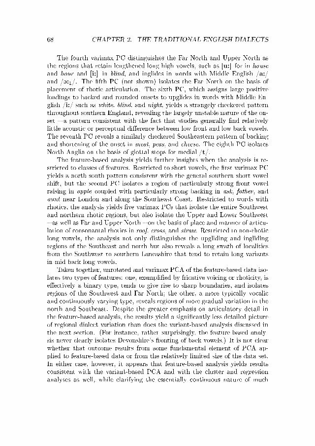
68 CHAPTER 2. THE TRADITIONAL ENGLISH DIALECTS
The fourth varimax PC distinguishes the Far North and Upper North asthe regions that retain lengthened long high vowels, such as [u:] for in houseand hour and [i:] in blind, and inglides in words with Middle English /a:/and /O:1/. The �fth PC (not shown) isolates the Far North on the basis ofplacement of rhotic articulation. The sixth PC, which assigns large positiveloadings to backed and rounded onsets to upglides in words with Middle En-glish /i:/ such as white, blind, and night, yields a strangely checkered patternthroughout southern England, revealing the largely unstable nature of the on-set � a pattern consistent with the fact that studies generally �nd relativelylittle acoustic or perceptual di�erence between low front and low back vowels.The seventh PC reveals a similarly checkered Southeastern pattern of backingand shortening of the onset in meat, peas, and cheese. The eighth PC isolatesNorth Anglia on the basis of glottal stops for medial /t/.
The feature-based analysis yields further insights when the analysis is re-stricted to classes of features. Restricted to short vowels, the �rst varimax PCyields a north-south pattern consistent with the general southern short vowelshift, but the second PC isolates a region of particularly strong front vowelraising in apple coupled with particularly strong backing in ask, father, andaunt near London and along the Southeast Coast. Restricted to words withrhotics, the analysis yields �ve varimax PCs that isolate the entire Southwestand northern rhotic regions, but also isolate the Upper and Lower Southwest� as well as Far and Upper North � on the basis of place and manner of articu-lation of consonantal rhotics in roof, cross, and straw. Restricted to non-rhoticlong vowels, the analysis not only distinguishes the upgliding and inglidingregions of the Southeast and north but also reveals a long swath of localitiesfrom the Southwest to southern Lancashire that tend to retain long variantsin mid-back long vowels.
Taken together, unrotated and varimax PCA of the feature-based data iso-lates two types of features: one, exempli�ed by fricative voicing or rhoticity, ise�ectively a binary type, tends to give rise to sharp boundaries, and isolatesregions of the Southwest and Far North; the other, a more typically vocalicand continuously varying type, reveals regions of more gradual variation in thenorth and Southeast. Despite the greater emphasis on articulatory detail inthe feature-based analysis, the results yield a signi�cantly less detailed pictureof regional dialect variation than does the variant-based analysis discussed inthe next section. (For instance, rather surprisingly, the feature-based analy-sis never clearly isolates Devonshire's fronting of back vowels.) It is not clearwhether that outcome results from some fundamental element of PCA ap-plied to feature-based data or from the relatively limited size of the data set.In either case, however, it appears that feature-based analysis yields resultsconsistent with the variant-based PCA and with the cluster and regressionanalyses as well, while clarifying the essentially continuous nature of much

2.7. PRINCIPAL COMPONENT ANALYSIS 69
Figure 2.8: Feature-Based Rotated Principal Components
(a) First Component (b) Second Component
(c) Third Component (d) Fourth Component
Note: Darker (lighter) shading indicates larger positive (negative) scores.
70 CHAPTER 2. THE TRADITIONAL ENGLISH DIALECTS
dialect variation.
2.7.2 Variant-Based Results
The variant-based PC analysis yields insights that di�er from but are largelycomplementary to those derived from the feature-based approach. Applied tothe variant-based data, the results of an unrotated PC analysis are di�cult tointerpret in linguistic terms, but varimax rotation yields a set of identifyingvariants for 12 regions that are largely congruent with most of the 15 regionsidenti�ed by the cluster and phylogenetic analyses. With appropriate caveats,in at least some cases the variants may arguably be said to characterize atraditional English dialect region.
The �rst rotated PC, whose largest positive loadings are presented in Table2.8 and whose component scores appear in Figure 2.9a, accounts for about 12percent of the variation in the data set. The map shows that the �rst PC largely� though not perfectly � overlaps with the broad Southwest dialect region,while the loadings reveal that the features most closely associated with the PCare the voicing of fricatives and occasionally of medial dentals, the plausiblyrelated voicing and dentalizing of medial fricative [s], and full lowering andunrounding of /u/.36 The PC also assigns high loadings to strong rhoticityas well as to a set of vocalic features that nearly fully describe a nonstandardregional dialect system of vowels, mainly involving the fronting of back vowels,development of (or even monophthongization to) a low-front onset in /i:/, andrelatively little raising of the low-front long vowels. However, those rhotic andvocalic features do not load as strongly in the PC because they are not asclosely correlated with it or with the highest-scoring features: [ó] is found ina much wider area than the Southwest, while most of the vocalic features arefound in narrower regions, predominantly in Devonshire � or in wider regionsthat only partially overlap with the Southwest. Thus the rhotic features arefound uniformly but not uniquely in the Southwest, while the vocalic ones arefound there uniquely but not uniformly.
36The historical origins of voicing of initial fricatives are poorly understood and, as voicingis found in Germanic dialects on the continent, may even extend to the earliest period ofAnglo-Saxon settlement in England. Whatever the case may be, it appears likely that voicingprevailed over much of southern England, including most localities south of a line extendingfrom mid-Shropshire to the Su�olk-Essex border, until as late as the 17th century and maynot have become considerably more restricted until the onset of industrialization in the early19th century. See Voitl (1988).

2.7. PRINCIPAL COMPONENT ANALYSIS 71
Figure 2.9: Variant-based Rotated Principal Components
(a) First Component (b) Second Component
(c) Third Component (d) Fourth Component
Note: Darker (lighter) shading indicates larger positive (negative) scores.

72 CHAPTER 2. THE TRADITIONAL ENGLISH DIALECTS
Table2.8:
Loadings:
First
Variant-based
Rotated
Principal
Com
ponent
LongVowels
ME/a:/
developsto
[e@∼
E@]in
theSouthwest(SAED
Map37)
0.645
ME/E:/
(<Old
English
/œ/,/ea/)shortened
to[E]in
Devonshire(SAED
Map54)
0.648
ME/E:/
(<Old
English
/œ/,/ea/)developsto
[Ei]throughtheSouth
andMidlands(SAED
Map51)
0.546
ME/e:/
issporadicallyshortened
to[I]in
9wordsin
theSouth
(SAED
Map48)
0.351
ME/i:/developsto
alow-frontorlow-centermonophthongin
Devonshire(SAED
Map21&22)
0.531
ME/i:/developsalow-frontorfrontonsetin
theSouthwest(SAED
Map21&22)
0.396
ME/O:
1/developsto
[Y:]in
Devonshire(SAED
Map74)
0.510
ME/O:
1/developsto
[w2
∼w
u]in
initialpositionin
3wordsin
theWestandNorth(SAED
Map71)
0.442
ME/O:
2/developsto
[Y:]in
Devonshire(SAED
Map74)
0.515
ME/o:/
developsto
[Y:]in
Devonshire(SAED
Map61)
0.589
ME/o:/
shortened
andfrontedto
[Y]in
Devonshire(SAED
Map18)
0.322
ME/u:/
developsto
[au]in
theWestMidlandsandlower
North(SAED
Map31)
0.545
ME/u:/
developsto
[EY]ontheedges
ofDevonshire(SAED
Map30)
0.405
ShortVowels
ME/a/+/f/,/T/,or/s/
becomes
lengthened
mainly
intheSouth
andMidlands
0.335
ME/o/+/f/,/T/,or/s/
lengthened
intheSouth
(SAED
Map9)
0.430
ME/o/+/f/,/T/,or/s/
typicallylowered
to[O
∼O:]mainly
intheSouth
0.321
ME/u/fullylowered
andunrounded
withtensenessto
[2 ˙]in
theSouthwest
0.863
Diphthongs
ME/au/developsto
acloser,more
rounded
[o –:]alongtheSouth
coast
(SAED
Map13)
0.718
ME/iu/developsto
[Y:]in
5wordsin
Devonshire(SAED
Map100B)
0.687
ME/Ou
/(<
Old
English
/aw/)developsto
[o:]in
theWest(SAED
Map96B)
0.480
ME/Ou
/(<
Old
English
/aw/)�naldevelopsto
[Ä]in
5wordsin
theSouthwestandSouthwestMidlands
0.340
ME/Ou
/(<
Old
English
/aw/)�nalremains[O
u]ordevelopsto
[I]in
5wordssporadically
0.320
Continued
onNextPage
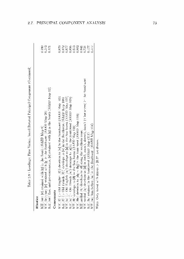
2.7. PRINCIPAL COMPONENT ANALYSIS 73
Table2.8:Loadings:
First
Variant-basedRotatedPrincipalComponent(Continued)
Rhotics
ME/ar/
[r]retained
with[ó]in
theSouth
(SAED
Map6)
0.580
ME/ir/-/
ur/
[r]retained
with[ó]in
theSouthwest(SAED
Map20)
0.512
ME/or/
�nalandpre-consonantal[r]retained
with[ó]in
theSouth
(SAED
Map12)
0.571
Consonants
ME/f/
(>Old
English
/f/)developsto
[v]in
theSouthwest(SAED
Map105)
0.970
ME/f/
(>Old
French
/f/)developsto
[v]in
theSouthwest(SAED
Map106)
0.872
ME/s/
(>Old
English
/s/)developsto
[z]in
theSouthwest(SAED
Map107)
0.977
ME/s/
(>Old
French
/s/)developsto
[z]in
theSouthwest(SAED
Map108)
0.896
ME/T/developsto
[D]in
theSouthwest(SAED
Map109)
0.973
ME/Tr/
developsto
[dó∼
Dó]in
theSouthwest(SAED
Map110)
0.962
MEmedial/t/
developsto
[d]alongthesoutherncoast
0.841
MEmedial/s/
developsto
[d]in
isn't,wasn't,doesn't,hasn't(4
instances)
intheSouthwest
0.721
ME/h/retained
intheSouthwest(SAED
Map(111)
0.477
ME/w/lost
before
/u/in
theSouthwest(SAED
Map114)
0.417
Note:Only
item
swithscores>|0.32|are
show
n.

74 CHAPTER 2. THE TRADITIONAL ENGLISH DIALECTS
The �rst PC suggests that the strongest candidates as identifying featuresof Southwestern speech are voicing of fricatives (and occasionally of medialdentals) and the full lowering and unrounding with tenseness of /u/. Otherfeatures with positive loadings are also diagnostic but not necessarily de�ning.That result is consistent with Trudgill's (1999) association of [z] in seven withthis dialect region.
Although it clearly identi�es a number of variants associated with the re-gion, neither the PC nor its associated variants is replicated perfectly in anysingle Southwestern locality, and they can only rather loosely be thought ofas representing a Southwestern dialect or even a group of dialects. Even thevoicing of fricatives appears in only about three-quarters of possible occur-rences in the Southwestern localities. Not even the most typical Southwesternlocality uses all of the variants with PC loadings above 0.32 in the �rst rotatedPC, and barely any of the localities even use a majority of them. Not muchmore than half of the variants associated with the PC occur even in the local-ity with the highest component score for the �rst PC; conversely, roughly 20percent of the variants occur in several of the lowest-scoring localities, whichtend to be somewhat further north in the West Midlands region. Moreover,the PC excludes a large number of variants that are widely used throughoutthe Southwest: strikingly, it does not include a single variant that is the mostcommon Southwestern pronunciation of a Middle English long vowel. Becausetheir distributions very rarely closely overlap with the boundaries of the South-west, most variants that might constitute a vowel system common to most ofthe Southwest do not in fact appear as part of the Southwestern PC. Suchlimitations appear to be inherent in the use of principal component or factoranalysis in the analysis of linguistic variation � and underline the fact thatsystematic variation is the exception rather than the rule in the traditionaldialects.
The second rotated PC, whose component scores are shown in Figure 2.9b,accounts for about 6 percent of the variation in the data set. It appears tobe strongly associated with most but not all of the Cumbria-North Yorkshiresubregion of the Upper North. The de�ning variants in this PC all involvethe development of a high front (and sometimes palatalized) onset plus schwafor /a:/, /O:1/, and /o:/, leading to their near-merger or even total merger.(The remainder of Cumbria-North Yorkshire is associated with PC 22 � notshown � which has many variants in common with the rest of the region butwhich tends to develop onsets in /e:/ and /u:/ and less fronting of the secondelement of /o:/.) While other variants also feature relatively strongly, thefronted onsets of several long vowels � not discussed at length by Trudgill �appear to be the most de�ning variants of the region. In contrast to the caseof the Southwest discussed previously, the second PC includes nearly all of thevariants that are the most common regional pronunciations of Middle English

2.7. PRINCIPAL COMPONENT ANALYSIS 75
long vowels. Still, by no means do all localities in the region use the de�ningvariants in the PC, and none use all of them. As with the �rst PC, only ratherloosely may the high-scoring variants in the PC be said to de�ne a dialect orgroup of dialects.
The third rotated PC, whose component scores are shown in Figure 2.9c,accounts for another 6 percent of the variation. The PC assigns high positiveloadings to several variants that very clearly delineate the Far North. Many ofthe localities in the region also have several other generally northern variants,including the fronting and palatalization of long back vowels discussed above.However, several variants are unique to the Far North, most importantly theuvular [K] but also the raising and fronting of the low back long vowels to [ø:](a full merger of both vowels to [ø:] is found only in the coastal localities),the fronting and occasional lengthening of /o/ to [œ ∼ œ:] and of /au/ to [a:∼ æ:], and the survival of [h] and [hw]. Again, although not all localities inthe region use all of them (and localities in the Upper North occasionally useseveral) these variants together can reasonably be said to de�ne the region �as indeed Trudgill does with [K], [h], and [hw]. As with the second PC, thethird includes nearly all of the variants that are the most common regionalpronunciations of the Middle English long vowels.
The fourth PC, accounting for about 4 percent of total variation, ratherweakly delineates most of East Anglia, as shown in Figure 2.9d. AlthoughTrudgill delineates and de�nes this region by its continuing use of [h] � a vari-ant that indeed scores fairly highly in the PC � the present analysis suggeststhat the development of [w] for /v/ and the development of a centered, un-rounded onset in /i:/ are somewhat more strongly associated with the region.Several more widely distributed variants coincide in East Anglia, particularlyin Norfolk, so that the region can be further associated with the unique occur-rence of those variants together � glottalized medial /t/, a fricative in aren'tyou, the fronting and unrounding of /o/, and the perhaps related raising of /a/� even though none of those variants score highly on the PC. The PC does notassign high loadings to any variants indicative of the moan/mown distinction,the fronting of /o/, the fear/fair merger, or the other variants known to becharacteristic of East Anglia; nor does it isolate many of the most commonEast Anglian variants of Middle English long vowels.
The �fth PC (not shown), accounting for about 4 percent of total variation,isolates the Severn Valley, essentially the southern half of the West Midlandssubregion of the Upper Southwest. The variant with the highest loading , thedevelopment of /au/ to [A:], points to a broader, related set of developmentsthat coincide in the region: a general lowering and unrounding of short backvowels, as well as at least occasional retraction and rounding of low short frontones. The region also develops diphthongs with high onsets (as well as center-ing or backing) in some words of the middle long vowel classes (that is, /E:/

76 CHAPTER 2. THE TRADITIONAL ENGLISH DIALECTS
and /O:1/) � a very long-standing dialect development. Otherwise, the middlelong vowels show relatively little movement, as in much of the west of Eng-land, perhaps contributing in the West Midlands to the relatively slight onsetsin the long high vowels. (Trudgill de�ned the region mainly in terms of theretraction and rounding of the vowel in land as well as the conservation of [a]in bat. The present analysis suggests that the former development is stronglycharacteristic in the region, but that [æ] is considerably more commonly usedthan [a].)
The sixth PC distinguishes Devonshire from the rest of the Southwest byits unique fronting of back vowels, a structural feature that appeared in the�rst PC as well: /O:1/, /O:2/, /o:/, and /iu/ all generally develop to [Y:], while/u:/ develops to [EY ∼ œu ∼ œY]. (Trudgill similarly points to the frontingof /o:/ in boot as the de�ning characteristic of Devonshire speech.) Anothervariant that is nearly as important is the development of a low monophthongfor /i:/.
The seventh PC distinguishes, to some extent, the unusual speech aroundthe �Potteries� zone in Sta�ordshire, Cheshire, and Darbyshire. Neighboringlocalities to the north and west tend to have raised monophthongs [e:] and[o:] for /a:/ and /O:/, respectively, while southern and eastern neighbors tendto have o�glides such as [ei] and [ou]. In the transition zone, localities tendto use [i:] and [u:], as though emphasizing both the raising of their northerlyneighbors and the o�glides of their southerly ones. The PC cannot be said todelineate a broad speech region or de�ne its variants, but it does �ag someof the de�ning variants of two neighboring regions. As mentioned previously,Trudgill notes Sta�ordshire and the surrounding regions as having an evenmore complete system that includes the variants mentioned above and severalmore besides. The present analysis suggests that there is so much variationamong localities in the region or that there is so much overlap of elements ofthe system with other regions that the complete system does not appear as aPC.
In the case of the eighth PC, the negative scores delineate and de�ne theSoutheast Coast and part of the Thames estuary. Here, the primary de�ningvariants involve a tendency to enhance the general Southern raising of shortfront vowels in at least some contexts. The rest of the important variantsappear to be manifestations of a tendency, systematic but by no means uni-form or universal throughout the Southeast, for long vowels to all develop intodiphthongs with rising o�glides, and many of the variants that take low tomoderate positive scores in this PC further re�ect that tendency. The presentanalysis did not include and therefore fails to note Trudgill's de�ning variantsfor parts of the Southeast Coast, namely the loss of /l/ at the end of wordsand the tendency to use [Ou] in words like old. It also fails to yield anotherperfectly reasonable way of characterizing the Southeast Coast � as the only

2.7. PRINCIPAL COMPONENT ANALYSIS 77
region that combines upgliding diphthongization of long vowels with retentionof rhoticity. Such a combination of variants is very unlikely to be capturedby principal component analysis because rhoticity and diphthongization eachoccur over very large regions with only a comparatively small area of overlap.
The negative scores of the ninth PC de�ne another region of the EnglishSoutheast � in this case the Central Southeast region around and to the northof London � by a process of diphthongization. The de�ning characteristicappears to be a tendency to front and lower the �rst elements of some ofthe diphthongs, such as [æi ∼ ai] for /a:/ and especially [@u ∼ 2u ∼ æu] for/O:1/. The results are consistent with the hypothesis that the diphthongizationis a long-term, ongoing process centered near the metropolis, and that olderforms are preserved in the periphery. (The fact that the progressive elementsare typically not found in American speech but regularly appear in English-speaking countries settled more recently may provide some con�rmation forthat hypothesis.) The analysis fails to capture the moan/mown distinctionnoted in this region by Trudgill.
The tenth PC delineates southern Lancashire, a portion of the Lower North,by the same variant noted by Trudgill � its localities' use of an alveolar ap-proximant rhotic. The eleventh PC rather poorly delineates the northern halfof the West Midlands, along with parts of the Lower North, by the retentionof a long monophthong for the low long vowels, as mentioned in the discussionof the seventh PC describing the transition zone between those regions andthe Midlands proper. The twelfth PC, characterized not only by the use ofthe retro�ex [ó] but by the tendency to insert it in such words as window,does not really delineate any dialect region, but it tends to take moderatelyhigh values through a broad swath of the Upper Southwest and the SoutheastCoast, tracing the southern edge of the major boundary of rhoticity in theSouth of England, the Wessex Line. The PC highlights the region of compe-tition between rhotic and non-rhotic variants, where rhotic speakers tend toovercompensate by inserting rhotics where they are otherwise absent.
The thirteenth PC clearly delineates Lincolnshire as the region which com-bines a tendency to develop a low-center onset to the high long vowels with atendency to develop centering diphthongs for the low and middle long vowels(and without strongly raising them). The fourteenth PC isolates and de�nessouth Yorkshire by its unique front upglides in the long low back vowels, andthe �fteenth does the same for north Lancashire and environs � the UpperNortheast � by its tendency to merge /O:1/ and /a:/ into a falling diphthong[ia ∼ ea]. Beyond those, the PCs appear increasingly uninformative from a lin-guistic point of view: the sixteenth isolates a dozen localities in the SoutheastCoast region that use a rhotic approximant; the seventeenth isolates a singlelocality on the Scottish border in Cumberland that uses a rhotic trill; and theeighteenth isolates some western localities that use a retracted, rounded vowel

78 CHAPTER 2. THE TRADITIONAL ENGLISH DIALECTS
in hand.In sum, PCA identi�es sets of identifying variants for a dozen-plus regions
largely congruent with many of the 15 regions identi�ed by the cluster andphylogenetic analyses, in the process accounting for roughly half the variationin the data set. In at least some cases, the PCs appear to provide a fairlyobjective method for characterizing the traditional English dialect regions ona quantitative basis. However, the PCs often isolate variants that are uniqueto a fairly small subregion, and they often include variants that are widely usedthroughout the relevant region but that are not unique to it. No locality in aregion uses all of the variants identi�ed by the relevant PC, and few even usemost of them. With the exception of three PCs that are composed of variantsfound in Devonshire, Lincolnshire, and the Far North, respectively, none ofthe PCs isolate extensive sets of variants that could be considered even partialsystems of vowels unique to particular regions of England.
2.7.3 Variant-based Principal Components and Variant
Frequency
Additional context for the results of the PC analysis can be derived by examin-ing the frequency of the two most common modern regional variants of most ofthe Middle English phonemes examined in this study. Regions do indeed tendto have fairly uniform speech patterns: the two most frequent variants in eachcategory account for at least 91 percent and as much as 98 percent of all usagein their respective regions. The most extensive intraregional variation occursamong long vowels and, to a lesser extent, diphthongs. The regions identi-�ed by distance measures, distance regressions, and variant-area regressionsas having the greatest variation � the Lower Northwest, the West Midlands,and the Central South � are the regions which have a large number of rel-atively low-frequency variants for the long vowels. With a few exceptions,variant usage for short vowels and consonants tends to be relatively uniformin each region. Although variant usage is relatively uniform within a givenregion, however, very few common variants are unique to a speci�c region: inthe great majority of cases variants are found in two or more regions. Thereis therefore relatively little scope for PC analysis to identify regions throughvariants that are unique to them. Nevertheless, even though any given varianttends to be found in a number of regions, each region has a relatively uniqueoverall pattern of frequently used variants.
These frequency details help explain the e�cacy and limitations of thePC analysis in identifying unique or important regional variants. The PCsdiscussed in the previous section identify many of the regionally most com-mon variants and nearly one-third of the regionally most common long vow-els and diphthongs. In three of the 15 regions � Cumbria-North Yorkshire,

2.8. CONCLUSIONS 79
Lincolnshire, and Devonshire, linguistically the most uniform regions � PCsassign high loadings to 8 of the 12 most common long vowels and diphthongs.However, in three other regions in the transitional center of the country �Sta�ordshire, the East Midlands, and the Central South � PCs fail to isolatea single one (though one PC identi�es a number of less common variants innorthern Sta�ordshire). Moreover, about one-third of the variants isolated bythe PC analysis are forms that are fairly uncommon even in the region or re-gions in which they appear. Equally importantly, only about one-quarter ofthe variants that appear in a PC and that are among the two regionally mostcommon variants for a Middle English phoneme can be more or less uniquelyassociated with a speci�c region: the remaining three-quarters are common inmore than one region, and in a number of cases they are identi�ed by morethan one PC in more than one region. For example, the development of alow-front or front onset (i.e. [ai ∼ Ei]) for Middle English /i:/ appears in thesecond PC as a characteristic of some importance in the Far North, where it isubiquitous. However, it also features in the third PC as a feature of marginalimportance in Cumbria-North Yorkshire, where it is also practically ubiqui-tous, and it surfaces yet again in the thirteenth PC as a feature of Lincolnshirespeech, where it appears with a frequency of 69 percent.
In short, PCs rarely isolate linguistic structures, variants, or features thatare unique to regions. Nevertheless they do tend to identify sets of variants orfeatures that are associated with regions, and a robust general characterizationof regional varieties of English usage emerges from the insights from the PCanalysis and an examination of the regional distribution of variants.
2.8 Conclusions
In summary, the quantitative tools presented here yield reasonable measuresof variation in phonetic usage among English localities, illustrate the largelycontinuous geographical nature of that variation (particularly with respect tovocalic features), identify a score of major and minor dialect regions as clus-ters of localities with relatively similar patterns of usage, distinguish regionsof relative uniformity from transitional zones with substantially greater varia-tion, and isolate regionally coherent groups of features that can be said � withappropriate caveats � to distinguish several but by no means all of the dialectregions. The results largely corroborate standard characterizations in the lit-erature, but di�er from those previous studies in several cases in the placementof several important dialect boundaries, in the association of features with di-alects, and in placing those systematic characteristics against a background oflargely continuous variation. The techniques reinforce each other to providea consistent picture of the traditional English usages, tending to con�rm the

80 CHAPTER 2. THE TRADITIONAL ENGLISH DIALECTS
applicability of computational techniques to the study of dialect variation.All of the techniques appear useful, though they need not all be used in
concert. The results suggest that even a small but judiciously chosen feature-based data set can yield a great deal of insight, and that in the absence offeature detail, variant-based data also can be used quite e�ectively. Clusteringtechniques are useful for delineating dialect regions, but they do not necessarilydistinguish between regions of greater uniformity and greater diversity � a taskfor which distance regressions, variant-area regressions, and barrier analysis aremore suitable, and any one of which is likely to be su�cient. Finally, principalcomponent analysis appears to be useful in identifying distinctive features orvariants that are more-or-less characteristic of dialect regions. The techniquemay be equally applicable to the study of linguistic variation across class,gender, and other dimensions as well. In some circumstances, feature-basedPCA may not only capture structural features such as upgliding or ingliding,but may provide measures of their strength, while variant-based PCA maycapture groups of variants that re�ect structural shifts. In this respect, feature-based and variant-approaches may be substitutes rather than complements.
Taken together, the results provide a phonetic basis for the following ten-tative classi�cation of the traditional English dialects and dialect regions, asre�ected in the usage of older rural speakers in the mid-twentieth century.
The relatively uniform Far North is distinguished from the rest of thecountry most notably by its use of uvular [K] � the Northumbrian burr. How-ever, the region also features the survival of [h] and [hw] � features that areoccasional but increasingly uncommon as one moves further south � as well asthe fairly common merger, raising, and fronting of the low back long vowelsto [ø:] and the fronting and occasional lengthening of /o/ to [œ ∼ œ:] andof /au/ to [a: ∼ æ:]. As in most of the north of England, the Middle Englishqualities of short vowels tend to be conserved.
The Upper North develops centering diphthongs for most of the longvowels. Cumbria-North Yorkshire is characterized by the development of ahigh front (and sometimes palatalized) onset plus inglide for /a:/, /O:1/, and/o:/, leading to a signi�cant degree of merger. The Upper Northwest shows asimilar development for /a:/ and /O:1/, except that the glides are to a lower,more fronted [a] rather than [@]. Both regions show the occasional developmentof /o:/ to [j7 ∼ iø].
The Lower North combines a tendency to develop the high long vowelsinto upglides with a low-center onset with a tendency to develop centeringdiphthongs for the low and middle long vowels without strongly raising them.The Lower Northwest is also characterized, in the west, by use of an alveolarapproximant rhotic, and in the east by fronted upglides in the long low backvowels. Lincolnshire has practically no unique features, save perhaps the merg-ing of /a:/ and /ai/ to [e@ ∼ E@], yet has a su�ciently unique and uniform

2.8. CONCLUSIONS 81
combination of variants that it can be clearly identi�ed by a variant-based PC.The Central Midlands sport such widely used and incoherently dis-
tributed variants and features that PC analysis cannot uncover de�nitive sets,but the region can generally be identi�ed by the unique overlapping of northernretention of older forms for the short vowels and the southeastern innovationsin the long vowels discussed below. The East Midlands � in many ways theheart of the English dialect world, with many of the most typical localities inthe SED and a highly uniform pattern of speech � never scores highly in anyprincipal component. Sta�ordshire appears as an island of relative uniformityin an important transition zone with unusual variability, but several techniquessuggest that a �Potteries� system is not evident the SED data, though princi-pal component analysis isolates a component of it in the northern part of theregion.
The Upper Southwest sees the most northerly expressions of severalsouthern characteristics, including rhoticity and short vowel shifts. The WestMidlands are characterized by a general lowering and unrounding of shortback vowels, occasional retraction and rounding of low short front ones, occa-sional high onsets in words with the middle long vowels, and little movementotherwise. The Central South proves to be a highly variable, transitional re-gion whose variants are in some cases too widespread and in other cases tooinfrequent to identify it. An examination of common features suggests thatthe Central South combines southern shifts in short vowels and retention ofrhoticity with minor northern tendencies to develop inglides in long vowels.
The Southeast sees extensive shifts in the Middle English short vowelsas well as the development of the Middle English long vowels into coherentsystems of upgliding diphthongs that are strongly evident in several of thevariant-based and feature-based principal components. North Anglia appearsbest de�ned by a hodgepodge of unique features, including glottalization ofmedial /t/, the development of [w] for /v/, the development of a centered,unrounded onset in /i:/, the continuing use of [h], but the analysis fails toidentify several other distinctively East Anglian features. The Central South-east is distinguished by the tendency to exaggerate the fronting and loweringof the �rst elements of some of the upgliding diphthongs, such as [æi ∼ ai]for /a:/ and especially [@u ∼ 2u ∼ æu] for /O:1/, while the Southeast Coastis distinguished by the tendency to enhance the general Southern raising ofshort front vowels in at least some contexts combined with retention of rhotic-ity; /l/-vocalization appears with relatively high frequency in the latter tworegions as well.
The Lower Southwest appears best de�ned by the voicing of fricativesand occasionally of medial dentals, the voicing and dentalizing of medial frica-tive [s], and full lowering and unrounding of /u/. Along with much of theUpper Southwest and the Southeast Coast, the Lower Southwest retains a

82 CHAPTER 2. THE TRADITIONAL ENGLISH DIALECTS
fully retro�ex rhoticity after vowels. The Central Southwest has little that isunique about it, tending to have features that overlap with those in neigh-boring regions, while Cornwall has little to distinguish it from the CentralSouthwest except its lower frequency of fricative voicing. Devonshire is distin-guished from the rest of the Southwest by its unique fronting of back vowelsand the development of a low monophthong for /i:/.
The neatness of these tentative classi�cations should not obscure the largelycontinuous and often unsystematic nature of phonetic variation across Eng-land. Even in regions with relatively uniform speech, few localities � not eventhose localities that can be characterized as having speech most typical oftheir regions � adhere rigidly to the patterns uncovered by any quantitativeapproach. Regional speech patterns appear to be only rather loosely char-acterized either by the patterns in their associated principal components, bythe speech patterns of their most typical localities, or by average frequenciesof occurrence of features. In linguistics as in biology, variation abounds, andtype specimens are necessarily arbitrarily chosen.