unrealistic expectations and misguided learning
TRANSCRIPT

http://www.econometricsociety.org/
Econometrica, Vol. 86, No. 4 (July, 2018), 1159–1214
UNREALISTIC EXPECTATIONS AND MISGUIDED LEARNING
PAUL HEIDHUESDüsseldorf Institute for Competition Economics, Heinrich–Heine Universität Düsseldorf
BOTOND KOSZEGIDepartment of Economics and Business, Central European University
PHILIPP STRACKDepartment of Economics, University of California, Berkeley
The copyright to this Article is held by the Econometric Society. It may be downloaded, printed and re-produced only for educational or research purposes, including use in course packs. No downloading orcopying may be done for any commercial purpose without the explicit permission of the Econometric So-ciety. For such commercial purposes contact the Office of the Econometric Society (contact informationmay be found at the website http://www.econometricsociety.org or in the back cover of Econometrica).This statement must be included on all copies of this Article that are made available electronically or inany other format.

Econometrica, Vol. 86, No. 4 (July, 2018), 1159–1214
UNREALISTIC EXPECTATIONS AND MISGUIDED LEARNING
PAUL HEIDHUESDüsseldorf Institute for Competition Economics, Heinrich–Heine Universität Düsseldorf
BOTOND KOSZEGIDepartment of Economics and Business, Central European University
PHILIPP STRACKDepartment of Economics, University of California, Berkeley
We explore the learning process and behavior of an individual with unrealisticallyhigh expectations (overconfidence) when outcomes also depend on an external funda-mental that affects the optimal action. Moving beyond existing results in the literature,we show that the agent’s beliefs regarding the fundamental converge under weak condi-tions. Furthermore, we identify a broad class of situations in which “learning” about thefundamental is self-defeating: it leads the individual systematically away from the cor-rect belief and toward lower performance. Due to his overconfidence, the agent—evenif initially correct—becomes too pessimistic about the fundamental. As he adjusts hisbehavior in response, he lowers outcomes and hence becomes even more pessimisticabout the fundamental, perpetuating the misdirected learning. The greater is the lossfrom choosing a suboptimal action, the further the agent’s action ends up from optimal.We partially characterize environments in which self-defeating learning occurs, andshow that the decisionmaker learns to take the optimal action if, and in a sense only if,a specific non-identifiability condition is satisfied. In contrast to an overconfident agent,an underconfident agent’s misdirected learning is self-limiting and therefore not veryharmful. We argue that the decision situations in question are common in economicsettings, including delegation, organizational, effort, and public-policy choices.
KEYWORDS: Overconfidence, learning, misspecified models, convergence, Berk–Nash equilibrium.
1. INTRODUCTION
LARGE LITERATURES in psychology and economics suggest that in many situations, indi-viduals have unrealistically positive beliefs about their traits or prospects, and researchershave began to investigate the nature of this “overconfidence” and to study its implica-tions for economic interactions.1 One important question concerning individuals withoverconfident or otherwise biased beliefs is how they update these beliefs when infor-mation comes in. Indeed, classical results identify conditions under which learning leads
Paul Heidhues: [email protected] Koszegi: [email protected] Strack: [email protected] are grateful to a co-editor, three anonymous referees, Roland Bénabou, Daniel Benjamin, Volker
Nocke, Demian Pouzo, and Francesco Squintani, as well as seminar and conference audiences for insightfulcomments and feedback. Heidhues and Koszegi thank the European Research Council for financial supportunder Starting Grant 313341. Part of this research was carried out while Heidhues and Koszegi visited theWissenschaftszentrum Berlin (WZB), which they thank for its hospitality. Mats Köster and Kinga Marczellprovided excellent research assistance.
1We use the term “overconfidence” to mean broadly any unrealistic beliefs, especially about ability or otherimportant personal characteristics, that lead a person to expect good outcomes. The same expression is oftenused more specifically to denote overly narrow confidence intervals (Moore and Healy (2008)). We reviewevidence for and theoretical work on overconfidence in Section 7.
© 2018 The Econometric Society https://doi.org/10.3982/ECTA14084

1160 P. HEIDHUES, B. KOSZEGI, AND P. STRACK
to correct beliefs (e.g., Savage (1954, Chapter 3)); more recent research explores ways inwhich a biased learning process can lead to overconfident beliefs (e.g., Gervais and Odean(2001), Chiang, Hirshleifer, Qian, and Sherman (2011), Jehiel (2017)).
In this paper, we investigate how overconfident individuals update not their overcon-fident beliefs, but their beliefs about other decision-relevant variables. Moving beyondexisting results in the literature, we show that beliefs converge under weak conditions.Furthermore, we identify a broad and economically important class of situations in whichan overconfident person’s inferences are self-defeating: they lead him systematically awayfrom the correct belief and toward lower performance. For example, if a team member isoverly full of himself and is hence disappointed by his team’s performance, he concludesthat his teammates are less talented or lazier than he thought. He responds by increasinghis control of the team, lowering team performance. He misinterprets this low perfor-mance as reflecting even more negatively on his teammates, perpetuating the misdirectedlearning further. Perversely, the greater is the loss from choosing a suboptimal action, thefurther the agent’s action ends up from optimal. We partially characterize environments inwhich self-defeating learning occurs, and show that the decisionmaker’s long-run behav-ior is optimal if and only if a specific non-identifiability condition is satisfied. In contrastto an overconfident agent, an underconfident agent’s misdirected learning is self-limitingand therefore not very harmful.
We present our framework in Section 2.1. In each period t ∈ {1�2�3� � � �}, the agentproduces observable output qt =Q(et� a�φ)+εt , which depends on his action et , his abil-ity or other output-relevant parameter a, an unknown fundamental φ, and a noise termεt . We assume that Q is increasing in a and φ, and that the optimal action is increasingin φ.2 The noise terms εt are independently and identically distributed mean-zero ran-dom variables with a log-concave distribution that has full support on R. The agent usesBayes’ rule to update beliefs, and chooses the myopically optimal action in every period(although in a special case, we analyze dynamically optimal actions as well). Crucially,the agent is overconfident: while his true ability is A, he believes with certainty that it isa > A. Finally, for most of the paper we assume that the optimal action depends in weaklyopposite ways on ability and the fundamental—that is, it is weakly decreasing in ability.This assumption is sufficient for generating self-defeating learning.
In Section 2.2, we argue that beyond team production, this reduced-form model cap-tures a number of economically important situations in which individuals may have un-realistic expectations. A principal may not know how intrinsically motivated his employ-ees are, and hence what level of control or explicit incentives maximizes performance.A person may not know how nice his partner or friend is, and hence how deferentially orassertively he should act to elicit the best outcomes from the relationship. A student oremployee may not know the return to effort, and hence how much effort is optimal. Ad-ditionally, a policymaker may not know the scale of underlying problems in the economy,and hence what policy leads to the best outcomes.
Adapting Esponda and Pouzo’s (2016a) concept of Berk–Nash equilibrium to our set-ting, in Section 2.3 we define a stable belief according to the intuitive consistency propertythat—when taking the action that he perceives as optimal given his false belief—the av-erage output the agent expects coincides with the average output he produces. Becauseat a stable belief the agent has no reason to question his beliefs, it is where his beliefs canbe expected to converge. Motivated by this observation, in Sections 3, 4, and 6 we studythe properties of stable beliefs, assuming that beliefs converge there; and in Section 5, we
2As long as these effects are monotonic, the above directional assumptions are just normalizations.

UNREALISTIC EXPECTATIONS AND MISGUIDED LEARNING 1161
take up convergence. We assume that there is a unique stable belief, and we identify suffi-cient conditions on the primitives for this to be the case (Proposition 1). This assumptionsimplifies our statements regarding the properties of limiting beliefs, and is crucial for ourconvergence proof.
In Section 3, we study the key properties of the agent’s learning process and limitingbeliefs, summarize a variety of casual evidence for our central mechanism, and discusseconomic implications. We establish that—as in the case of the overconfident team mem-ber above—the agent’s learning process is self-defeating: if his initial action is not toofar from optimal, then the opportunity to change his action in response to what he learnsleads to more incorrect beliefs, and more suboptimal behavior, than if he could not changehis action (Proposition 2). Furthermore, limiting beliefs satisfy a surprising and perversecomparative static: the more important it is for the agent to take the right action—that is,the greater is the loss from a suboptimal action—the further his beliefs end up from thetruth, and the further his behavior ends up from optimal (Proposition 3). Intuitively, whenchoosing a suboptimal action is more harmful, the agent hurts himself more through hismisguided learning. To develop a consistent theory of his observations, therefore, he mustbecome more pessimistic about the fundamental.
We also consider what happens if—similarly to a dissatisfied team member decidingwhether to replace his teammate—the agent can choose between the above task and anoutside option. Consistent with the literature on overconfidence, the agent might be tooprone to enter into and initially persist in the task. In contrast to received wisdom, how-ever, our model predicts that the agent’s growing pessimism about the fundamental mayinduce him to exit the task too easily (Proposition 4), and by implication to jump too muchbetween tasks. This prediction is consistent with the observation that many documentedeffects of overconfidence in economic settings, such as the pursuit of mergers and innova-tions by overconfident chief executive officers (CEOs) or the creation of new businessesby overconfident entrepreneurs, pertain to new directions.
In Section 4, we ask what happens when our sufficient condition for self-defeatinglearning—that the optimal action depends in opposite ways on ability and the funda-mental—is not satisfied, and we argue that self-defeating learning still occurs if and onlyif the optimal action depends sufficiently less on ability than on the fundamental. As aconceptually interesting case, we show that long-run behavior is always optimal if, and ina sense we will make precise only if, Q has the form V (e�S(a�φ))—that is, ability andthe fundamental are not separately identifiable (Proposition 5). This conclusion contrastswith the lesson from classical learning settings that non-identifiability hinders efficientlearning. Intuitively, because ability and the fundamental do not have independent ef-fects on output, the agent’s misinference about the fundamental can fully compensate hisoverconfidence, and hence in the long run overconfidence does not adversely affect him.If his team’s output depends on his effort and the team’s total ability, for instance, theagent correctly infers total ability, and chooses effort optimally.
In Section 5, we show that if Q satisfies some regularity conditions, then the agent’sbeliefs converge to the stable belief with probability 1 (Theorem 1). Furthermore, un-der the additional assumption that Q is linear in φ, beliefs converge to the stable beliefeven when actions are dynamically optimal (Theorem 2). To prove convergence, we can-not apply results from the statistical learning literature, such as those of Berk (1966) andShalizi (2009), where the observer does not choose actions. Worse, beliefs constitute afunction-valued process, whose transitions are, due to the endogeneity of the agent’s ac-tion, driven by shocks that are neither independently nor identically distributed. Littleis known in general about the asymptotic behavior of the posterior distribution in such

1162 P. HEIDHUES, B. KOSZEGI, AND P. STRACK
infinite-dimensional models when the observations are not independently and identicallydistributed (i.i.d.), even when the model is correctly specified (e.g., Ghosal and van derVaart (2007, pp. 192–193)). To get a handle on the problem, we employ a method that toour knowledge has not been used in the literature on learning with misspecified models.We focus on the agent’s extremal beliefs: what levels of the fundamental does he in thelimit conclusively rule out? Given the structure of our problem, this puts bounds on hislong-run actions, which restrict his extremal beliefs further. Using this contraction logic,we show that the agent rules out everything but a single point.
Knowing that beliefs converge with probability 1 allows us to make another economi-cally relevant point: given that in the long run the agent correctly predicts average output,his beliefs pass a specification test based on comparing the empirical distribution of noiseterms he estimates to the true distribution (Proposition 6). In this sense, the agent’s over-confidence is—even with infinite data—stable.
In Section 6, we analyze variants of our framework using a simple output function of theformQ(e�a�φ)= a+φ−L(e−φ) for a symmetric loss function L. We consider a settingin which the agent is initially uncertain about a, and observes—in addition to output—anoisy signal of his relative contribution to output, a − (φ − L(et − φ)). It being highlysubjective, however, the agent observes his own contribution with a positive bias. As aresult, he develops overconfidence about a, and his limiting belief about φ is identical tothat in our basic model (Proposition 7).
We also study underconfident agents (for whom a < A), and identify an interestingasymmetry: while an overconfident agent’s limiting utility loss from misguided learningcan be an arbitrarily large multiple of his overconfidence a−A, an underconfident agent’slimiting utility loss is bounded by his underconfidence A− a (Proposition 8). To under-stand the intuition, consider an underconfident agent who starts off with the correct meanbelief about the fundamental. Upon observing higher levels of output than he expected,the agent concludes that the fundamental is better than he thought, and he revises hisaction. The resulting utility loss, however, leads him to reassess the optimistic revision ofhis belief, bringing his beliefs back toward the true fundamental. Hence, his misinferenceregarding the fundamental—which with overconfidence was self-reinforcing—is now self-correcting.
In Section 7, we relate our paper to the two big literatures it connects, that on the impli-cations of overconfidence and that on learning with misspecified models. From a method-ological perspective, our model is a special case of Esponda and Pouzo’s (2016a) frame-work for games when players have misspecified models. Because we have an individual-decisionmaking problem with a specific structure, we can derive novel and economicallyimportant results that are not possible in the general framework. In particular, to ourknowledge our paper is the first to study the implications of overconfidence for inferencesabout other decision-relevant variables, and how these inferences interact with behavior.We are also unaware of other papers that characterize when self-defeating learning doesversus does not occur in an individual-decisionmaking context.
In Section 8, we conclude by discussing some potential applications of our frameworkfor multi-person situations.
2. LEARNING ENVIRONMENT
In this section, we introduce our basic framework, outline possible economic applica-tions of it, and perform a few preliminary steps of analysis.

UNREALISTIC EXPECTATIONS AND MISGUIDED LEARNING 1163
2.1. Setup
In each period t ∈ {1�2�3� � � �}, the agent produces observable output qt =Q(et� a�Φ)+εt ∈ R, where et ∈ (e� e) is his action, a ∈ R is his unchanging ability, Φ ∈ (φ�φ) is an un-observable unchanging fundamental, and εt is random noise. Throughout the paper, wemake the following basic assumptions. First, the state Φ is drawn from a continuous priordistribution π0 : (φ�φ)→ R>0 with finite moments and bounded positive density every-where on (φ�φ), and we suppose that the agent has the correct prior belief π0. Second,the εt are i.i.d. continuously distributed mean-zero random variables. Denoting their cu-mulative distribution function by F and their strictly positive density by f : R → R>0, weimpose a version of log-concavity: the second derivative of log f is strictly negative andbounded from below.3 Third, output satisfies some regularity properties and normaliza-tions: Q is twice continuously differentiable, with it and its derivates having polynomialgrowth inφ, and (i)Qee < 0 andQe(e�a�φ) > 0>Qe(e�a�φ) for all a�φ, (ii)Qa�Qφ > 0,and (iii) Qeφ > 0.4 Part (i) guarantees that there is always a unique myopically optimal ac-tion. Part (ii) implies that output is increasing in ability and the fundamental, and part (iii)implies that the optimal action is increasing in the fundamental. As long as the effects im-plied by parts (ii) and (iii) are monotonic, our directional assumptions on them are justnormalizations, and do not affect the logic and message of our results. Indeed, if any ofthese derivatives was negative, we could change variables to reverse the orientation of a,φ, or e, and obtain a model in which the same derivative is positive.
We assume for most of the paper that the agent chooses his action myopically in eachperiod, aiming to maximize that period’s expected output. This assumption is irrelevantfor our analysis of the properties of stable (point) beliefs in Sections 3, 4, and 6. We douse the assumption for our main convergence result, although under stronger conditionswe establish convergence also when the agent optimizes dynamically.
Crucially, we posit that the agent is overoptimistic about his ability: while his true abilityis A, he believes with certainty that it is a > A. Let Δ= |A− a| denote the degree of theagent’s overconfidence. Given his inflated self-assessment, the agent updates his beliefsabout the fundamental in a Bayesian way. To guarantee that the agent can always find afundamental that is consistent with the average output he produces, we assume that forall e, there is a φ ∈ (φ�φ) such that Q(e�A�Φ)=Q(e� a� φ). Note that because Qφ > 0,this φ is unique.
We specify the agent’s belief about ability as degenerate for two main reasons. Techni-cally, the assumption generates a simple and tractable model of persistent overconfidence,allowing us to focus on our research question of learning about other variables. Moreimportantly, we view an assumption of overconfident beliefs that are not updated down-ward as broadly realistic. Quite directly, such an assumption is consistent with the view ofmany psychologists that individuals are extremely reluctant to revise self-views downward(e.g., Baumeister, Smart, and Boden (1996)). More generally, such an assumption can be
3We think of strict bounded log-concavity as an economically weak restriction: it guarantees that an increasein output increases the agent’s belief about the fundamental in the sense of the monotone likelihood ratioproperty, and that any signal is nontrivially informative. Examples of distributions that have full support onR and satisfy the assumption include the normal and logistic distributions. Technically, it also ensures thatsubjective beliefs are well defined and have finite moments after any history (see Lemma 3 in the Appendix).
4A function J(e�a�φ) is of polynomial growth in φ if for any e�a, there are κ�k�b > 0 such that|J(e�a�φ)| ≤ κ|φ|k + b for all φ. This assumption ensures that expected output and its derivatives exist af-ter any history (see Proposition 9 in the Appendix).

1164 P. HEIDHUES, B. KOSZEGI, AND P. STRACK
thought of as a stand-in for forces explored in the psychology and economics literatures(but not explicitly modeled here) that lead individuals to maintain unrealistically positivebeliefs. To show that our model is consistent with this perspective, in Section 6.1 we allowfor the agent to be uncertain about a, and show that a biased learning process leads to asetting essentially equivalent to ours.5
To complete the description of our model, we state a sufficient condition for self-defeating misguided learning to occur.
ASSUMPTION 1—Sufficient Condition for Self-Defeating Learning: We havesgn(Qea) �= sgn(Qeφ).
Note that with the normalization Qeφ > 0, Assumption 1 is equivalent to Qea ≤ 0. Thisassumption plays a central role in our paper: in Section 3, we explore the implications ofmisguided learning under Assumption 1, and in Section 4, we study what happens whenAssumption 1 is not satisfied. Given our results—especially the analysis and discussion inSection 4—economically we think of Assumption 1 as allowing for two possibilities:
(i) The optimal action is almost insensitive to ability, at least relative to how sensitiveit is to the fundamental (Qea ≈ 0 �Qeφ). This is likely to be the case in many applicationsin which the agent is looking to fine-tune a decision—such as the design of a public policyor organizational incentive system—to circumstances he views as largely external to hisability.
(ii) In small-scale economic settings, however, the optimal action may be nontriviallysensitive to ability. Then, Assumption 1 requires that the optimal action depends in oppo-site ways on ability and the fundamental. This assumption naturally holds for delegation,as the optimal extent of delegation depends in opposite ways on the decisionmaker’s abil-ity and his teammate’s ability. In contrast, the assumption does not hold if output alwaysdepends on ability and the fundamental in similar ways, such as when it depends on a+φ.
The following two parametric examples are useful to keep in mind when developingour results.
EXAMPLE 1—Loss-Function Specification: The output function has the form
Q(e�a�φ)= a+φ−L(e−φ)� (1)
where e=φ= −∞, e=φ= ∞, a ∈ R, and L is a symmetric loss function with L(0)= 0and |L′(x)| < k < 1 for all x. The agent observes output in each period, but does notobserve output gross of the loss L(et −Φ) nor the loss itself. Economically, this specifica-tion captures a situation in which the agent wants to adjust his action to some underlyingstate of the world. Researchers have used similar, loss-function-based, specifications inCrawford and Sobel (1982) and the large literature on cheap talk, expert advice, andorganizations (e.g., Alonso, Dessein, and Matouschek (2008)) following it, as well as inMorris and Shin (2002) and the subsequent literature on coordination.
5The model in Section 6.1 replaces a misspecified point belief about a with misspecified learning about a,and hence is also not a fully rational model. But we view the misspecified nature of the agent’s learning asa feature, not a bug: any model in which the agent is correctly specified and keeps learning until he has thecorrect belief about his ability contradicts observed widespread overconfidence among individuals who havehad plenty of opportunity to learn about themselves.

UNREALISTIC EXPECTATIONS AND MISGUIDED LEARNING 1165
EXAMPLE 2—Effort Specification: The output function has the form
Q(e�a�φ)= (a+ e)φ− c(e)� (2)
where e = φ = 0, e = φ = ∞, a > 0, and c is a strictly convex cost function withc(0) = c′(0) = 0, and lime→∞ c′(e) = ∞. In this example, the action e is effort, and thefundamental φ determines the return to effort. The agent observes output, and may alsoobserve output gross of the cost of effort; since he knows his level of effort, the two ob-servations provide the same information to him.
Consistent with our motivating phenomenon of overconfidence, in describing and dis-cussing our model and results we interpret a as ability. But more broadly, a could standfor any variable that leads the agent to be steadfastly and unrealistically optimistic abouthis prospects. For example, he may have overly positive views about his country or orga-nization, or, as in the case of policymakers below, he may have overly optimistic beliefsabout the technology generating output.
2.2. Applications
In this section, we argue that several economically important settings fit our model inSection 2.1. In each of these settings, other individuals are also involved, and for a fullaccount it is necessary to model their behavior as well. Nevertheless, to focus on a singleagent’s inferences and behavior, we abstract from the decisions of others, and model theireffect only in reduced form.
APPLICATION 1—Delegation: The decisionmaker is working in a team with anotheragent and must decide how much of the work to delegate. The expected output ofthe team is Q(e�a�φ) = au(e) + φv(e), where e ∈ (0�1) is the proportion of the jobthe decisionmaker delegates, φ is the teammate’s ability, and a�φ > 0, u(e)� v(e) > 0,u′(e)�u′′(e)� v′′(e) < 0, and v′(e) > 0. Then, the higher is the decisionmaker’s ability andthe lower is the teammate’s ability, the lower is the optimal extent of delegation.
APPLICATION 2—Control in Organizations: A principal is deciding on the incentivesystem to use for an agent who chooses two kinds of effort, overt effort xo (e.g., writingreports) and discretionary effort xd (e.g., helping others in the organization). The prin-cipal can incentivize overt effort, for instance through monitoring (e.g., requiring andreading reports) or explicit incentives written on an objective signal of overt effort. Forsimplicity, we assume that the principal chooses xo directly. Consistent with the litera-ture on multitasking starting with Holmström and Milgrom (1991), we also assume thatdiscretionary effort is a decreasing function of overt effort. In addition, we suppose thatdiscretionary effort is an increasing function of the agent’s intrinsic motivation φ. Writingdiscretionary effort as xd = xd(xo�φ), the principal’s profit is R(a�xo�xd(xo�φ)), wherea is the quality of the organization, the principal’s ability, or other factor affecting overallproductivity. Supposing that the optimal overt effort is decreasing in intrinsic motivation,this model reduces to our setting with Q(e�a�φ)=R(a�−e�xd(−e�φ)).6�7
6One simple functional form capturing our discussion is R(a�xo�xd(xo�φ)) = a + xo + xd(xo�φ), where
the discretionary effort function satisfies ∂xd(xo�φ)∂xo
< 0� ∂xd(xo�φ)∂φ
> 0, and ∂2xd(xo�φ)∂xo∂φ
< 0.7An alternative interpretation of the same framework is that xo is the agent’s “mechanical” input into the
organization, xd is his “creative” input, and φ is his ability. In this interpretation, creative input depends oncreative effort—which is a substitute to overt effort—and ability.

1166 P. HEIDHUES, B. KOSZEGI, AND P. STRACK
APPLICATION 3—Assertiveness Versus Deference: The decisionmaker is in a personalrelationship—such as partnership or friendship—with another individual. The output qis how “nicely” the other person is acting, including how willing she is to comply withthe agent’s requests, how much of the unpleasant joint work she does, and so forth. Thefundamental φ is how nice the other person is, and e is how deferentially the agent actstoward her. This action could range from being extremely deferential (high e) to beingextremely aggressive or even violent (low e). Finally, a stands for the agent’s talent orattractiveness. Output is determined according to the loss-function specification of Ex-ample 1: the partner tends to act more nicely if she is a nicer person, if the agent is moretalented or attractive, and if the agent’s behavior is more attuned to the partner’s niceness.
Of course, the deference or aggressiveness of an agent, or the niceness of hispartner’s behavior, are not typical outcomes studied by economists. But these areclearly observable—with noise—to individuals, and manifestations—at least of extremechoices—might be observable to researchers as well.8
APPLICATION 4—Work and Return to Effort: The agent is an employee or student whomust decide how hard to work at his job or school. He periodically observes the output ofhis efforts, such as promotions, grades, or other rewards, but he does not know the returnto effort. Output is given by the effort specification in Example 2.
APPLICATION 5—Public Policy: A policymaker aims to maximize the performance ofsome aspect of the economy, q, which depends on his policy choice e, a fundamentalφ, hisability or his party’s or country’s potential a, and noise according to the loss-function spec-ification in Example 1. In particular, output q could be the well-being of the populationin relation to drug-related crime, φ could be the underlying condition of the populationwith respect to drug use, and e could be the degree of drug liberalization. The extent of re-strictions must be optimally aligned with underlying conditions to minimize drug-relatedcrime. In a completely different example, q could represent the overall performance ofthe economy, e could represent the country’s openness toward other countries in trade,exchange of ideas, and movement of people, and φ could represent the optimal degree ofintegration with the world economy.9
One may argue that since politicians are heavily scrutinized and receive a lot of feed-back, they should learn about themselves and not be overconfident. Yet by extensivelydocumenting and studying overconfidence in another high-flying and heavily scrutinizedgroup, top CEOs, Malmendier and Tate (2005) and the literature following it have shownthat feedback does not necessarily eliminate overconfidence. Hence, while we are un-aware of direct compelling evidence that politicians are overconfident, it is plausible thatmany are. In addition, a policymaker may have unrealistic expectations not only becauseof his trust in himself, but also because of his unrealistic beliefs about policy tools. Hemay, for instance, have false beliefs about how much of an increase in economic growthor reduction in crime can be achieved with the right policy.
2.3. Preliminaries
Let e∗(φ) denote the optimal action when the fundamental is φ. We define the surprisefunction as
�(φ)=Q(e∗(φ)�A�Φ)−Q(e∗(φ)� a�φ
)� (3)
8For instance, Card and Dahl (2011) study the role of emotions in family violence using police records.9This example was suggested to us by Francesco Squintani.

UNREALISTIC EXPECTATIONS AND MISGUIDED LEARNING 1167
If the agent believes the fundamental to be φ, then he takes the action e∗(φ), and there-fore expects average output to beQ(e∗(φ)� a�φ). In reality, he obtains an average outputofQ(e∗(φ)�A�Φ), so that �(φ) represents the average surprise he experiences. ApplyingEsponda and Pouzo’s (2016a) Berk–Nash equilibrium—their solution concept for gameswhen players may have misspecified models—to our setting, yields the following defini-tion.10
DEFINITION 1: A stable belief is a Dirac measure on a fundamental φ∞ at which theagent is not surprised by average output, that is, �(φ∞)= 0.
Given our assumption of a full-support prior, a stable belief is the only type of pointbelief that the agent may find no reason to abandon. If the agent holds a stable beliefabout the fundamental, then he takes an action such that he produces on average exactlyas much as he expects, confirming his belief. In contrast, if the agent holds any other pointbelief about the fundamental, then he takes an action such that he obtains a nonzeroaverage surprise, accumulating evidence that the fundamental is something else. As aresult, one would expect the agent’s beliefs to converge to a stable belief, if one exists.
Motivated by these observations, in the rest of the paper we perform two distinct typesof analysis. In Sections 3, 4, and 6, we study properties of the agent’s stable beliefs, assum-ing that his beliefs converge to a stable belief. And in Section 5, we confirm in the centralcase of our model that—under somewhat stronger technical assumptions—beliefs indeedconverge to a stable belief.
For our analysis, we assume that there is a unique stable belief. Although our model’smechanism and insights regarding the properties of stable beliefs hold more generally,this assumption simplifies many of our statements. In addition, the assumption is crucialfor our convergence proof. We identify sufficient conditions for a unique stable belief asfollows.
PROPOSITION 1: There is a unique stable belief if any one of the following statementsholds:
(i) Derivative Qa is bounded, derivative Qφ is bounded away from zero, and overconfi-dence (a−A) is sufficiently small.
(ii) Output Q takes the form in Example 1.(iii) Output Q takes the form in Example 2 and c′′′(e)≥ 0.
3. MAIN MECHANISM AND ECONOMIC IMPLICATIONS
In this section, we lay out the main forces in our model, and discuss economic impli-cations. For this purpose, we suppose that Assumption 1 holds. Although we state ourresults for general Q, throughout we use the loss-function specification of Example 1 forillustration. For these illustrations, we normalize A=Φ= 0, and suppose that the prioron φ is symmetric and has mean equal to the true fundamental.
3.1. Self-Defeating Learning
3.1.1. Example 1. Fixed Action
As a benchmark case, we suppose for a moment that et is exogenously given and con-stant over time at level e= e∗(Φ)= 0. Then, average output converges toQ(e�A�Φ)= 0.
10Lemma 7 in the Appendix shows formally that a stable belief and the corresponding optimal action con-stitute a Berk–Nash equilibrium, and that every pure-strategy Berk–Nash equilibrium is of that form.

1168 P. HEIDHUES, B. KOSZEGI, AND P. STRACK
FIGURE 1.—Limiting beliefs with fixed action.
The agent, in turn, believes that if the state is φ, then average output is Q(e� a�φ) =a+ φ− L(e− φ) = a+ φ− L(φ). To explain an average output of zero, therefore, hecomes to believe that the fundamental is φe∞ satisfying a+φe∞ −L(φe∞)= 0.
Figure 1 illustrates. The agent’s belief about the fundamental (φ) as well as his action(e) are on the horizontal axis, and output is on the vertical axis. The agent’s limiting beliefis given by the intersection of the loss function through the origin and the line a+φ: atthis point, the loss from taking the (in his mind) suboptimal action exactly explains theaverage output of zero.
Clearly, φe∞ < Φ. Intuitively, the agent is surprised by the low average output he ob-serves, and concludes that the fundamental is worse than he thought. This tendency toattribute failures to external factors provides a formalization of part of the self-servingattributional bias documented by Miller and Ross (1975) and the literature following it.Indeed, one account of the bias is that individuals have high expectations for outcomes,and update when outcomes fall short (Tetlock and Levi (1982), Campbell and Sedikides(1999)). But while the agent’s inference about the fundamental is misguided—it takeshim away from his correct prior mean—in the current setup with a fixed action it is harm-less or potentially even beneficial. For instance, because the agent now correctly predictsaverage output, he makes the correct choice when deciding whether to choose this taskover an outside option with a given level of utility.11
3.1.2. Example 1. Endogenous Action
Now suppose that the agent chooses his action optimally given his beliefs. We illustratethe learning dynamics in Figure 2, again putting the agent’s belief (φ) as well as his action(e) on the horizontal axis and putting output on the vertical axis. The “average output pos-sibilities curve” Q(e�A�Φ)= −L(e) represents true average output as a function of theagent’s action, and the “perceived average achievable output line”Q(e∗(φ)� a�φ)= a+φrepresents the average output the agent believes is reachable as a function of the funda-
11As a simple implication, if the agent’s high belief about ability is due to ego utility as in Koszegi (2006), thenmisdirected learning allows him to have his cake and eat it too: he can maintain the pleasure from believingthat his ability is high, while not suffering any losses associated with incorrect beliefs.

UNREALISTIC EXPECTATIONS AND MISGUIDED LEARNING 1169
FIGURE 2.—Learning with endogenous action.
mental φ. Since e∗(φ)=φ, the agent’s stable belief assigns probability 1 to the intersec-tion of the two curves. It is apparent from the figure that the limiting belief is furtherthan in the case of exogenously fixed actions above. Hence, learning is self-defeating ina basic sense: the fact that the agent can optimize given his learning makes his learningeven more inaccurate, with the corresponding bad effect on his actions. In particular, theagent’s limiting per-period utility loss relative to the optimal action can be an arbitrarilylarge multiple of his overconfidence Δ.
How does the agent drive himself into such a highly suboptimal situation? We give aheuristic argument, assuming that the agent updates his action increasingly rarely, andpretending that his average output and beliefs reach their limit in finite time after eachupdate. Suppose that for a long time, the agent chooses the optimal action given his initialbeliefs, e= 0, and ends up with an average output of zero. Then, the belief φ1 he developsabout the fundamental is the same as in the case of exogenously fixed actions: it is givenby the intersection of the loss function starting at (0�0) (the higher dashed curve L(φ))and the perceived average achievable output line.
Now suppose that the agent updates his action, and for an even longer time keeps tak-ing the optimal action given his new belief, e = φ1. Then, he ends up with an averageoutput of −L(φ1). To identify the φ2 consistent with this average output, we draw a copyof the loss function starting from his current action-average output location (the lowerdashed curve L(φ − φ1) − L(φ1)), and find the intersection of this curve with the per-ceived average achievable output line. This is his new belief φ2 (which, therefore, satisfiesa+φ2 − L(φ2 −φ1) = −L(φ1)). Continuing with this logic gives a sense of the agent’slearning dynamics, and illustrates why he ends up at φ∞.

1170 P. HEIDHUES, B. KOSZEGI, AND P. STRACK
We briefly discuss how our prediction of self-defeating learning can manifest itself in theapplications outlined in Section 2.2. In the context of manager–subordinate relationships(an example of Application 1), Manzoni and Barsoux (1998, 2002) describe a commonproblem—the “set-up-to-fail syndrome”—that is due to a dynamic similar to our mecha-nism. When the subordinate performs below expectations, the manager reacts by increas-ing control and assigning less inspiring tasks. This undermines the employee’s motivation,lowering performance and eliciting further negative reactions from the manager.
In the context of organizations (Application 2), the notion of dysfunctional viciouscircles has been described in sociology (March and Simon (1958), Crozier (1964),Masuch (1985)). Management is dissatisfied with the performance of the organizationand attempts to improve things with increased monitoring, control, or other bureaucraticmeasures. These measures backfire, for instance, because they alienate employees. Man-agement reacts by tightening bureaucratic measures further.
In the context of personal relationships (Application 3), our model provides one possi-ble mechanism that links unrealistically high self-views to aggressive behavior. Althoughit had been hypothesized that aggression is associated with low self-esteem, Baumeister,Smart, and Boden (1996) and the subsequent literature reviewed by Lambe, Hamilton-Giachritsis, Garner, and Walker (2018) argue that aggressive individuals tend to have highself-esteem that is not based on compelling facts. Our model says that in this situation,the agent comes to feel that his partner does not treat him with the respect he deservesfrom a nice partner, and reacts by becoming more assertive. As a result of this misguidedreaction, he receives even less respect from his partner, leading him to react even morestrongly. The relationship deteriorates, and potentially ends up abusive and/or violent.12
Although we have not found discussions that are reminiscent of our mechanism in ourother applications, self-defeating interpretations of worse-than-expected outcomes alsoseem plausible in these settings. In the context of work or study effort (Application 4),when a person with unrealistic expectations does not obtain the rewards he expects, heconcludes that the return to talent and effort is lower than he thought, and he lowers hiseffort in response. But because effort is important, this lowers his output more than heexpects, leading him to become even more pessimistic about the return to effort. As acase in point, our mechanism may contribute to the widespread underestimation of thereturns to college education documented by Bleemer and Zafar (2018), but more researchis necessary to determine the extent and nature of its role.
In an interesting contrast to our model, existing work on overconfidence, such asBénabou and Tirole (2002), Gervais, Heaton, and Odean (2011) and de la Rosa (2011),has emphasized that if ability and effort are complements, then overconfidence can bene-fit a person by leading him to exert higher effort. Our model says that if ability and efforthave separable effects, or even if they are complements, but the complementarity is low,then exactly the opposite is the case.
In the context of the war on drugs (an example of Application 5), a policymaker mayinterpret drug problems as indicating that he should crack down on drugs, only to makethe problem worse and the reaction harsher. In the context of nationalism, policymakers(or citizens) may react to disappointing economic outcomes by concluding that globaliza-tion does not hold as much promise as they had hoped. This leads the country to adopt
12The mechanism that Baumeister and coauthors describe verbally is somewhat different from ours. Theyhypothesize that violence serves as a way for a person to protect his unrealistically high self-views when theseviews are threatened by an outsider. While this is consistent with our mechanism if we interpret a “threat”as treating the agent with less respect than he believes he deserves, the relationship of the two mechanismswarrants further research.

UNREALISTIC EXPECTATIONS AND MISGUIDED LEARNING 1171
more nationalistic and protectionist policies, exacerbating the problem and hardening theconclusion that globalization is a failure.
3.1.3. General Q
We now state the self-defeating nature of learning formally and for general Q.
PROPOSITION 2: Suppose Assumption 1 holds. If the agent’s action is exogenously fixedat e ≥ e∗(Φ), then his beliefs converge to a Dirac measure on a point φe∞ satisfying φ∞ <φe∞ <Φ.
Proposition 2 implies that if the agent starts off with an action at or above the optimalaction, then the opportunity to change his action in response to his inferences leads tomore incorrect long-run beliefs than if he could not change his action. By continuity, thesame is the case if his initial action is below but close to the optimal action. Of course, theself-defeating nature of learning also implies that if the initial action is not too far fromthe optimal action, then the opportunity to update his action lowers the agent’s long-runaverage utility.
We conclude this section by illustrating in the loss-function specification that the direc-tional assumptions we have made on the effect of the fundamental on output and the op-timal action (Qφ�Qeφ > 0) are indeed irrelevant for the logic of our results. First, supposethat the production function is of the form Q(e�a�φ)= a−φ−L(e−φ), so that an in-crease in the fundamental lowers expected output. As Figure 3 makes clear, this leaves the
FIGURE 3.—Learning when the fundamental lowers output.

1172 P. HEIDHUES, B. KOSZEGI, AND P. STRACK
logic—including that the agent’s learning is self-defeating and can leave his beliefs arbi-trarily far from the truth relative to Δ—completely unchanged: the average output possi-bilities curve is still −L(e), and the perceived average achievable output line is now a−φ,so the mirror image of our previous analysis applies. Consider also the possibility that theoptimal action depends negatively on the state (Qeφ < 0):Q(e�a�φ)= a+φ−L(e+φ).With the trivial change of variables φ′ = −φ, this is equivalent to the case above, so onceagain the same analysis and the same insights result.
3.2. The Importance of Being Right
3.2.1. Example 1
Because it provides a surprising and potentially testable prediction of our model, weconsider the comparative statics of stable beliefs with respect to the loss function. Anincrease in the loss function increases the agent’s incentive to act in accordance withthe fundamental. His action responds in an unfortunate way: by ending up further fromthe fundamental. If the loss function shifts up, then the curve −L(e) in Figure 2 shiftsdown, and the stable belief φ∞ therefore moves to the left. Intuitively, a steeper lossfunction means that the agent hurts himself more through his misinferences. To developa consistent theory of his observations, therefore, he must become more pessimistic aboutthe world.
3.2.2. General Q
To generalize the above result to arbitrary production functions, we define
R(a�φ)=Q(e∗(a�φ)�a�φ)�
L(e�a�φ)=Q(e∗(a�φ)�a�φ)−Q(e�a�φ)�
(4)
and observe that Q(e�a�φ) = R(a�φ) − L(e�a�φ). Intuitively, R(a�φ) is the averageachievable output given a and φ, and L(e�a�φ) is the loss relative to the achievableoutput due to choosing a suboptimal action. We compare two technologies Q1 and Q2
with corresponding e∗1, e∗
2, R1, R2, L1, and L2.
PROPOSITION 3: Suppose Assumption 1 holds, e∗1(a�φ) = e∗
2(a�φ) and R1(a�φ) =R2(a�φ) for all a�φ, and L1(e�a�φ) < L2(e�a�φ) for all a�φ�e �= e∗(a�φ). Then, theagent’s stable belief is further below the true fundamental Φ under technology Q2 than undertechnology Q1.
The key step in the proof of Proposition 3 is that an increase in the loss function de-creases the surprise function. An increase in the loss function means that the agent hurtshimself more through his misinference-induced suboptimal behavior, and this must meanthat he is more negatively surprised by his average output. Additionally, a downward shiftin the surprise function lowers the agent’s stable belief.
3.3. Outside Options
In the above model, we have assumed that the agent participates in the task in everyperiod regardless of his beliefs. It is natural to consider an environment in which he has anoutside option, such as another task he could perform. In the manager–employee setting,

UNREALISTIC EXPECTATIONS AND MISGUIDED LEARNING 1173
for instance, a manager can keep working with the current employee, or he can fire theemployee and reopen or discontinue the position.
Let the utility of the outside option be u. We suppose that the agent correctly under-stands u, and discuss the implications of relaxing this assumption below. We denote by Φthe prior mean of the fundamental, and by φ∞ the stable belief when the fundamentalis Φ. Let ut = maxe
∫Q(e� a�ψ)πt−1(ψ)dψ be the utility the agent assigns to the task ac-
cording to the belief he holds at the beginning of period t, πt−1. The agent chooses the out-side option in period t if and only if ut < u. We assume that Q(e∗(φ∞)� a� φ∞) < u < u1,which is the situation in which interesting new issues arise. As Proposition 4 below shows,in this case the overconfident agent starts off by choosing the task, but as the prior be-comes sufficiently concentrated, the probability that he eventually switches to the outsideoption approaches 1.
There are then two cases defined by how a realistic agent behaves. If u >maxe∫Q(e�A�
ψ)π0(ψ)dψ, then a realistic agent would not enter the task in the first place, so an over-confident agent’s entry into it and his initial persistence in it are both suboptimal. Theprediction that overconfident individuals—overestimating their ability to perform well—are more likely to enter into and persist in ability-sensitive tasks is consistent with commonintuition and evidence from psychology as well as economics. Overconfidence is often in-voked as one explanation for why many new businesses fail in the first few years, andindeed Landier and Thesmar (2009) find that entrepreneurs of small startups have over-confident expectations about future growth. Similarly, several studies suggest that CEOoverconfidence is associated with a higher likelihood of pursuing risky actions, such asmaking acquisitions (Malmendier and Tate (2008)) and undertaking innovation (Galassoand Simcoe (2011), Hirshleifer, Low, and Teoh (2012)). And persisting in tasks (oftenfor too long) is regarded as one of the main characteristics of overconfidence (McFarlin,Baumeister, and Blascovich (1984), for example).
More novel and surprising insights emerge if u <maxe Q(e�A� Φ).
PROPOSITION 4: Suppose that Qφ < κφ and Q(e∗(φ∞)� a� φ∞) < u <maxe Q(e�A� Φ).As the variance of π0 approaches 0:
(i) The probability that the overconfident agent eventually switches to and then sticks withthe outside option approaches 1.
(ii) The probability that a realistic agent ever chooses the outside option approaches 0.
Given that the outside option is relatively poor, the agent should start off choosing thetask, and given that the prior variance is small, sticking with the task is likely to be therational strategy. Yet the overconfident agent is likely to suboptimally give up on the task.Ironically, therefore, the agent stops performing the task because he overestimates hisability to do well in it. Intuitively, he is more prone to exit than a realistic agent becausehis negative inferences about the fundamental eventually negate his overconfidence.
Importantly, an overconfident agent is prone to overestimate not only output in thecurrent task, but—in as much as it depends in part on ability—also the outside option u.Such overestimation exacerbates the tendency to exit the task, and can generate interest-ing dynamics when there are multiple types of alternative tasks for the agent to choose.The logic of our model suggests that the agent first seeks out another ability-sensitive taskin which he believes a different fundamental determines outcomes, and then successively

1174 P. HEIDHUES, B. KOSZEGI, AND P. STRACK
jumps from one such task to the next. And once he runs out of these tasks, he chooses aless ability-sensitive task and sticks with it.13
The prediction that overconfidence leads individuals to eventually quit superior tasks,to jump too much between tasks, and to eventually prefer less ability-sensitive tasks, con-trasts with the typical view on the implications of overconfidence. While we have notfound direct evidence for this prediction, it is consistent with the observation that manydocumented effects of overconfidence in economic settings, such as the tendency of over-confident CEOs to undertake mergers or innovations, pertain to the pursuit of new direc-tions rather than to persistence in old directions.
Our result that an overconfident agent jumps between tasks suggests one possible rea-son for the persistence—though not for the emergence—of overconfidence. Since theagent often abandons tasks and prefers tasks for which previous learning does not apply,he can keep updating mostly about external circumstances, slowing down learning abouthis ability.
4. WHEN LEARNING IS NOT DETRIMENTAL
In Section 3, we have shown that self-defeating learning—whereby the agent’s responseto his misguided inferences leads to even more misguided inferences and even more sub-optimal behavior—always occurs under Assumption 1. We now discuss what happenswhen Assumption 1 is not satisfied, allowing us to partially characterize the conditionsthat facilitate self-defeating learning.
Suppose, therefore, that Qea > 0, so that the optimal action is strictly increasing inability. To understand the key issue, suppose also that the agent starts off with a beliefthat is concentrated around the true fundamental. Then, because he is overconfidentand Qea > 0, his initial action is too high. As in the rest of our analysis, the surpris-ingly low average output he observes leads him to revise his belief about the fundamentaldownward—and, as a consequence, to choose lower actions. Because his initial action wastoo high, this adjustment is in the right direction. We then have two cases. It is possiblethat in the limit misdirected learning increases output, so that self-defeating learning doesnot occur. It is, however, also possible that misdirected learning lowers the action belowoptimal, at which point the logic by which further learning occurs is analogous to that inSection 3. Then, self-defeating learning may occur: any further negative inference aboutφ leads the decisionmaker to choose lower actions, lowering output and reinforcing hisnegative inference.
As a conceptually interesting question, as well as to say more about when each of theabove two cases obtains, we ask when a misspecified agent’s long-run behavior is optimal.Call the action that is optimal given the unique stable belief the stable action.
PROPOSITION 5: The following statements are equivalent:(i) For any A, a, and Φ, the agent’s stable action is optimal (i.e., maximizes true expected
output).(ii) There is a function V (e�S(a�φ)) such that (a) for any A, a, and Φ, the agent’s
stable action is identical to that with the output function Q(e�a�φ) = V (e�S(a�φ)), and(b) VS�Sa� Sφ > 0, and for any a, φ, and a, there is a unique φ′ satisfying S(a�φ)= S(a�φ′).
13A related point to ours is made in a bargaining context by Bénabou and Tirole (2009), who show that anindividual may leave a productive partnership in part because he overestimates his outside option. Our modelpredicts that the agent may well exit even if he correctly understands the outside option. As a result, he mayexit even if no ability-sensitive alternative tasks are available.

UNREALISTIC EXPECTATIONS AND MISGUIDED LEARNING 1175
Proposition 5 says that agents with wrong beliefs about ability always (i.e., for any A,a, and Φ) behave optimally in the long run if and only if there is an output function thatalways describes long-run behavior and that depends only on a summary statistic S ofability and the fundamental, and not independently on the two variables. With such anoutput function, the agent can in the limit correctly deduce S from average output, sohe correctly predicts how changes in his action affect output. As a result, he chooses theoptimal action. Our proof establishes that this kind of production function is not onlysufficient, but in the above sense is also necessary for learning to be optimal in the limit.
An interesting aspect of Proposition 5 is that the agent is able to find the optimal ac-tion exactly when the problem is not identifiable—that is, when his observations of outputdo not allow him to separately learn a and φ. This beneficial role of non-identifiabilityis in direct contrast to what one might expect based on the statistical learning literature,where non-identifiability is defined as a property of the environment that hinders learn-ing. Yet it is exactly the non-identifiability of the problem that allows the overconfidentagent to choose his long-run action well: because ability and the fundamental do not haveindependent effects on output, the agent’s misinference about the fundamental can fullycompensate his overconfidence regarding ability, and hence overconfidence does not ad-versely affect him.
In the team production setting, for instance, suppose that the agent—instead of makingdelegation decisions—chooses his effort level, and that output depends on effort and thetotal ability of the team (i.e., output takes the form V (e�a+φ)). Then, although the agentstill underestimates his teammates, he is able to deduce the team’s total ability a+φ fromoutput. As a result, he chooses the optimal action.
Notice that statement (ii) of Proposition 5 implies that controlling for their ef-fect on output, the optimal action is equally sensitive to ability and the fundamental(e∗a(a�φ)/Qa(e
∗(a�φ)�a�φ) = e∗φ(a�φ)/Qφ(e
∗(a�φ)�a�φ)). This insight indicates thatif Qea > 0, then changes in the agent’s beliefs about the fundamental eventually in-duce actions that are significantly lower than optimal—and, hence, self-defeating learningoccurs—if the optimal action is sufficiently more sensitive to the fundamental than to abil-ity. Adding our insights from Section 3, we conclude that self-defeating learning occurs ifthe optimal action either (i) depends sufficiently less on ability than on the fundamentalor (ii) depends in opposite ways on ability and the fundamental.
5. CONVERGENCE
In this section, we establish conditions under which the agent’s beliefs converge to thestable belief. We also argue that when the agent’s beliefs converge, his overconfidence isstable—that is, he will not realize he is wrong—in a specific sense.
5.1. Convergence With Myopic Actions
To establish convergence, we maintain the same assumptions as in Section 2.1, but im-pose stronger conditions on some of the derivatives of Q.14
ASSUMPTION 2: We have (i) |Qe|< κe, (ii) Qa ≤ κa, 0< κφ ≤Qφ ≤ κφ, and (iii) |Qφφ| ≤κφφ.
14Example 1 satisfies Assumption 2 as long as L′′ is bounded. Example 2 does not satisfy Assumption 2 asstated, but it does so under economically minor modifications: that e <∞, φ<∞, and a is positive, bounded,and bounded away from zero.

1176 P. HEIDHUES, B. KOSZEGI, AND P. STRACK
The various bounds in Assumption 2 guarantee that the agent’s inferences from outputand his reactions to these inferences are always of comparable size.15
Our main result in this section is the following theorem.
THEOREM 1: Suppose Assumptions 1 and 2 hold. Then, the agent’s beliefs almost surelyconverge in distribution to the unique stable belief φ∞, and his actions almost surely convergeto e∗(φ∞).
The interdependence between actions and beliefs—that the agent’s action depends onhis belief, and the bias in his inferences in turn depends on his action—creates severaldifficulties in our convergence proof. To start, we cannot apply results from the statisticallearning literature, such as those of Berk (1966) and Shalizi (2009), where the observerdoes not choose actions. Even one central necessary component of the convergence of be-liefs, the concentration of beliefs, requires some properties of the path of actions. Indeed,convergence does not hold in some other models with endogenous actions, such as thoseof Nyarko (1991) and Fudenberg, Romanyuk, and Strack (2017), and the convergence re-sult of Esponda and Pouzo (2016a, Theorem 3) applies only for priors close to the stablebelief and for actions that are only close to optimal. To make matters especially difficult,beliefs constitute a function-valued process whose transitions are driven by shocks that areneither independently nor identically distributed. In general, the asymptotic behavior ofthe posterior distribution in such infinite-dimensional models when the observations arenot i.i.d. is not well understood, even when the model is correctly specified (e.g., Ghosaland van der Vaart (2007, pp. 192–193)).
To resolve this problem, we apply a technique that to our knowledge has not beenused in the literature on learning with misspecified models. We focus on extremal beliefs:what levels of the fundamental does the agent in the limit conclusively rule out? Giventhe structure of our problem, this puts bounds on his long-run actions, which restrict hisextremal beliefs further. Using this contraction argument, we show that the agent rulesout everything but the root of �.
We explain the detailed logic of our proof in six steps.Step 1. We show that the change in beliefs can in the long run be approximated well by
the expected change. To argue this, we use that the log-likelihood function is the averageof the log-likelihoods of the realized outputs. This is the technically most demanding stepin the proof, as—due to the endogeneity of actions—the log-likelihood is an average ofnonidentical and nonindependent random variables. We adapt existing versions of the lawof large numbers to the types of non-i.i.d. random variables our framework generates.
Step 2. We establish that if the agent is on average positively surprised by output forbelief φ, then by Step 1 the derivative of his subjective log-likelihood goes to infinityalmost surely at φ. An analogous statement holds for negative surprises.
Step 3. If the agent has realistic beliefs about ability (a = A), then—no matter hisaction—his average surprise is positive for φ < Φ, and negative for φ > Φ. By Step 2,his beliefs converge to Φ almost surely.
Step 4. Now we turn to the overconfident agent. We define φ∞ as the supremum offundamentals such that in the long run, the agent almost surely convinces himself that the
15Specifically, the lower bound on Qφ ensures that the agent always makes a nontrivial inference from anincrease in output. The upper bound on Qφ bounds how much the agent learns from the output of a singleperiod. Similarly, the bounds on Qe and Qa ensure that changing the action or ability has a limited effecton output. The condition on Qφφ helps us to bound the second derivative of the subjective posterior log-likelihood.

UNREALISTIC EXPECTATIONS AND MISGUIDED LEARNING 1177
true fundamental is above φ∞. We define φ∞ analogously. We show that the beliefs ofan overconfident agent can be bounded—in the sense of the monotone likelihood ratioproperty—relative to the beliefs of a realistic agent. Using that the beliefs of a realisticagent converge to Φ, this means that φ∞ and φ∞ exist. And because the agent is over-confident, his beliefs about the fundamental must in the long run be below the truth:φ∞ ≤φ∞ ≤Φ. The goal for the rest of the proof is to show that φ∞ =φ∞ =φ∞.
Step 5. We show that the above bounds on long-run beliefs also bound long-run actions.In particular, we know that the optimal action is increasing in the fundamental. There-fore, in the long run the agent’s action must be on (or arbitrarily close to) the interval[e∗(φ∞)� e
∗(φ∞)].Step 6. Now we show by contradiction that φ∞ ≥ φ∞. Supposing that φ∞ < φ∞, we
establish that the agent’s average surprise at φ∞ is positive in the long run. To see this,note that because φ∞ < φ∞, the average surprise is positive for the action e∗(φ∞). Fur-thermore, since the agent overestimates ability and underestimates the fundamental (andQea ≤ 0�Qeφ > 0), he underestimates Qe. This implies that the agent’s average surprise ispositive for any action near or above e∗(φ∞), that is, for any long-run action. By Step 2,in the long run the agent convinces himself that the fundamental is above, and boundedaway from, φ∞, contradicting the definition of φ∞. An analogous argument establishesthat φ∞ ≤φ∞.
5.2. Convergence With Dynamically Optimal Actions When Q Is Linear in φ
In Section 5.1, we established convergence by assuming that the agent takes the myopi-cally optimal action. In the current section, we consider dynamically optimal actions. Weassume that the agent has discount factor δ ∈ (0�1), and in each period chooses a cur-rent action and a (history-contingent) strategy for future actions to maximize discountedexpected output. Because et affects how much the agent learns about the fundamental,the myopically optimal action is in general not dynamically optimal, making it difficult tobound actions based on beliefs. For example, the agent will take an action associated witha low payoff this period if that action reveals a lot of information about optimal futureactions. Nevertheless, we establish convergence in a special case of our model.
ASSUMPTION 3: Suppose (i) Q(e�a�φ)=φH(e�a)+G(e�a), (ii) the second derivativeof log f is bounded away from zero, (iii) the prior distribution π0 of Φ satisfies −∞< κπ ≤(∂2/∂φ2) logπ0(φ)≤ κπ <∞ as well as φ≥ 0 and π0(φ)= 0, and (iv) et is chosen from abounded interval.
The substantive new assumption is (i), which says that average output is linear in φ.The other assumptions are regularity conditions that add to Assumption 2.16
THEOREM 2: Suppose Assumptions 1, 2, and 3 hold, and the agent chooses dynamicallyoptimal actions. Then, the agent’s beliefs almost surely converge in distribution to the uniquestable belief φ∞, and his actions almost surely converge to e∗(φ∞).
16The output function of Example 2 is linear in the fundamental and thus the example satisfies Assumption 3as long as e is bounded. Example 1 does not satisfy Assumption 3.

1178 P. HEIDHUES, B. KOSZEGI, AND P. STRACK
To understand the key new idea, notice that for any et , the agent believes that
φ+ εt
H(et� a)= qt −G(et� a)
H(et� a)�
Hence, the agent believes that the observations (qt − G(et� a))/H(et� a) are indepen-dently distributed signals with mean φ, albeit with a variance that depends on et . By thelogic underlying the law of large numbers, the agent’s subjective beliefs therefore concen-trate in the long run for any sequence of actions. This implies that the subjective expectedbenefit from learning about the fundamental Φ vanishes, so the agent must eventuallychoose actions that are close to myopically optimal. As a result, the logic of Theorem 1applies.
5.3. Stability of Overconfidence
A central assumption of our paper is that the agent has an unrealistically high pointbelief about his ability. In this section, we ask whether his observations might lead him toconclude that something about his beliefs is awry, which might lead him to reconsider hisbelief about ability.17 We show that if beliefs and actions converge, then there is a strongsense in which the agent will see no reason to doubt his belief about ability, even after hehas observed infinite data.
To make our point, we construct a specification test for the agent’s beliefs that—in addi-tion to relying on infinitely many observations—is arguably far more stringent than whata person would realistically submit his views to. Formally, suppose that the agent’s beliefsconverge to the stable belief. Given this limiting belief, the agent looks back and extractsthe noise realizations he thinks have generated his observations: εt = qt −Q(et� a�φ∞).Now the agent takes the infinite subsample {εt1� εt2� � � �} of the εt , where t1� t2� � � � arespecified ex ante. Let Fi(x) = |{i′ ≤ i|εti′ ≤ x}|/i be the empirical frequency of observa-tions below x in the first i elements of his subsample. The agent expects this empiricalcumulative distribution to match the true cumulative distribution of εt in the long run, itdoes.
PROPOSITION 6: Suppose that beliefs converge in distribution to the unique stable belief.Then, for any sequence ti and any x, limi→∞ Fi(x)= F(x).
Intuitively, in the long run the agent settles on beliefs that lead him to predict averageoutput accurately, so that he also extracts the noise terms accurately. Hence, he cannotbe surprised about the long-run distribution of noise terms.
It is worth noting the role of the convergence of actions—as distinct from the conver-gence of beliefs—in our result. Suppose, for example, that the agent is forced to take eachof the two actions e1 and e2 > e1 infinitely many times at prespecified dates, but at vanish-ing rates, so that his beliefs still converge to φ∞. Since a > A and φ∞ <Φ, Qeφ > 0 andQea ≤ 0 imply that Qe(e�A�Φ) > Qe(e� a�φ∞). The agent therefore underestimates thedifference in average output with e2 versus e1, and hence Proposition 6 fails in a strongway: the empirical mean of εt must be nonzero either at e1 or at e2. This example illus-trates that the informational environment makes it possible for our specification test to
17See Gagnon-Bartsch, Rabin, and Schwartzstein (2017) for a more detailed exploration of when a personwith a misspecified model may discover that he is wrong.

UNREALISTIC EXPECTATIONS AND MISGUIDED LEARNING 1179
fail—but the agent takes actions under which it does not. In particular, his action doesnot vary enough for him to reject his belief about ability.
Of course, one may imagine a more sophisticated specification test that hinges on thespeed of convergence of the agent’s beliefs. Unfortunately, we are unable to determinewhether the agent passes such a test, because our convergence proofs cannot say anythingabout the speed of convergence, not even in the case of a realistic agent. We are skeptical,however, that a typical economic agent would perform specification tests of such sophis-tication.18
6. EXTENSIONS AND MODIFICATIONS
In this section, we discuss some economically relevant variants of our model. For sim-plicity, we restrict attention to the loss-function specification of Example 1 throughoutthis section. In addition, as in Sections 3 and 4, we assume that beliefs converge to theDirac measure on the root of the surprise function, and study only properties of limitingbeliefs.
6.1. Biased Learning About Ability
Throughout the paper, we have assumed that the agent holds a point belief about abilitythat is too high, thinking of this assumption as a stand-in for forces that generate overcon-fidence. We now show through a simple example that the mechanisms we have identifiedare consistent with a setting in which overconfidence arises endogenously through biasedlearning. Although the precise bias we assume is different, one can think of this exerciseas integrating Gervais and Odean’s (2001) model of “learning to be overconfident” withour model of misdirected learning.
Suppose that the agent has continuously distributed prior beliefs about (a�φ) with fullsupport on the plane. In each period, he observes output qt = a+φ−L(et −φ)+ εt aspreviously. In addition, he observes a noisy measure of his relative contribution to output,rt = a− (φ−L(et −φ)+ εt)+ ε′
t +Δ′, where the ε′t have mean zero. However, the agent
perceives his relative contribution with a bias: while he believes that Δ′ = 0, in realityΔ′ = 2Δ.
The assumption that individuals perceive their own contribution to performance in a bi-ased way is supported by a variety of evidence in psychology. For instance, Ross and Sicoly(1979) find that when married couples are asked about the portion of various householdchores they perform, their answers typically add up to more than 100 percent. Babcockand Loewenstein (1997) provide evidence that parties in a negotiation interpret the sameinformation differently and in a self-serving way. Summarizing the literature, Bénabouand Tirole (2016) explain that selective attention to and recall of information, asymmetricinterpretation of information, and asymmetric updating can all contribute to individuals’biased self-evaluations. Our model captures these possibilities in one simple reduced-form way.
Logically, it is possible that the agent evaluates not only rt , but also qt in a biased way.But in most situations motivating our analysis, a person’s contribution to output is more
18Similarly, if noise is not additively separable from Q, then the agent’s belief may fail a variant of thedistribution-based test in Proposition 6. Even this conclusion, however, hinges on the agent being certain aboutthe distribution of noise. If he is not certain, then the long-run distribution of output may lead him to makeinferences about the noise distribution rather than to conclude that his belief about ability is incorrect.

1180 P. HEIDHUES, B. KOSZEGI, AND P. STRACK
subjective than output itself, and is hence more vulnerable to distortion. Bénabou andTirole (2009) make a similar distinction.
Because the agent now observes both qt and rt , we redefine his surprise function forthis two-dimensional case. If the agent believes that his ability is a and the fundamental isφ, then he takes the action φ. We therefore write
�q(φ�a)= [A+Φ−L(φ−Φ)]− [a+φ]�
�r(φ�a)= [A− (
Φ−L(φ−Φ))+Δ′]− [a−φ]�The first line is the agent’s surprise function for output, which follows the same logicas in our basic model. The second line is the agent’s surprise function for his relativecontribution. Due to his bias, the average relative contribution the agent perceives isA−(Φ − L(φ − Φ)) + Δ′. But because he is not aware of his bias, he expects his averagerelative contribution to be a−φ. Setting both surprises to zero, adding, and rearranginggives that the stable belief about ability must be a∞ =A+Δ′/2 =A+Δ—exactly the pointbelief that we imposed exogenously in our basic model. Plugging this into the unchangedsurprise function for output, we get that the stable belief about the fundamental must alsobe the same as in our basic model.
PROPOSITION 7: There is a unique stable belief a∞�φ∞, where a∞ =A+ Δ= a and φ∞is the unique root of � defined in Equation (3).
Intuitively, the agent believes that the average of total output and his relative contribu-tion,
∑t(qt + rt)/2, provides an unbiased estimate of his ability. This estimator, however,
converges to A+ Δ, so that he develops overconfident beliefs over time. Given that hebecomes overconfident about ability, he is misled about the fundamental in the same wayas in our basic model.
6.2. Underconfidence
While many or most people are overconfident, some are “underconfident”—they haveunrealistically low beliefs about themselves. We briefly discuss the implications of under-confidence for misguided learning. In Figure 4, we redraw the relevant parts of Figure 2for underconfident beliefs (a < A), again normalizingA andΦ to 0. As for overconfidentagents, any possible stable belief is given by the intersection of the average output pos-sibilities curve −L(e) and the perceived average achievable output line a+φ. If a < A,the two curves intersect to the right of the true fundamental: since the agent is pessimisticabout his own ability, he becomes overly optimistic about the fundamental. Furthermore,it is apparent from the figure that in the limit the agent’s loss from underconfidence isbounded by Δ. The formal statement follows.
PROPOSITION 8: Suppose Q takes the loss-function form in Example 1 and a < A. Then,there is a unique stable belief φ∞, which satisfies 0<φ∞ −Φ<Δ and L(φ∞ −Φ)< Δ.
These results contrast sharply with those in the overconfident case, where the limitingbelief is always more than Δ away from the true fundamental (Φ − φ∞ > Δ), and theassociated loss can be an arbitrarily large multiple of Δ. To understand the intuition, con-sider again an agent who has a symmetric prior with mean equal to the true fundamental.

UNREALISTIC EXPECTATIONS AND MISGUIDED LEARNING 1181
FIGURE 4.—Limiting belief and loss with underconfidence.
Due to his underconfidence, the agent is then likely to observe some better performancesthan he expects. As a result, he concludes that the fundamental is better than he thought,and he revises his action. The resulting utility loss, however, leads him to reassess theoptimistic revision of his belief, bringing his beliefs back toward the true fundamental. Inthis sense, the agent’s misinference regarding the fundamental is self-correcting—in con-trast to the logic in the case of overconfidence, where the misinference is self-reinforcing.Moreover, because a utility loss of Δ or more cannot be explained by a combination ofunderconfidence in the amount of Δ and an unrealistically positive belief about the fun-damental (which increases expected output), any consistent belief must generate a utilityloss of less than Δ.
7. RELATED LITERATURE
Our theory connects two literatures, that on overconfidence and that on learning withmisspecified models. While we discuss other more specific differences below, to ourknowledge our paper is the first one to study the implications of overconfidence for in-ferences about other, decision-relevant exogenous variables. More recently, Le Yaouanqand Hestermann (2016) study the same question, focusing on the issue of persistence,which we cover only briefly in Section 3.3. We are also unaware of previous research thatcharacterizes when self-defeating learning does versus does not occur in an individual-decisionmaking context.

1182 P. HEIDHUES, B. KOSZEGI, AND P. STRACK
7.1. Overconfidence
Our paper studies the implications of unrealistic expectations regarding a variable forlearning about another variable. In many applications, the most plausible source of suchunrealistic expectations is overconfidence, which is the topic of an extensive literature ineconomics and psychology.
A plethora of classical evidence in psychology as well as economics suggests that onaverage people have unrealistically positive views of their traits and prospects (e.g.,Weinstein (1980), Svenson (1981), Camerer and Lovallo (1999)). Recently, Benoît andDubra (2011) have argued that much of this evidence is also consistent with Bayesianupdating and correct priors, and thus does not conclusively demonstrate overconfidence.In response, a series of careful experimental tests have documented overconfidence inthe laboratory in a way that is immune to the Benoît–Dubra critique (Burks, Carpen-ter, Goette, and Rustichini (2013), Charness, Rustichini, and van de Ven (2018), Benoît,Dubra, and Moore (2015)). In addition, there is empirical evidence that consumersare overoptimistic regarding future self-control (Shui and Ausubel (2004), DellaVignaand Malmendier (2006), for instance), that truck drivers persistently overestimate fu-ture productivity (Hoffman and Burks (2017)), that genetically predisposed individu-als underestimate their likelihood of having Huntington’s disease (Oster, Shoulson, andDorsey (2013)), that unemployed individuals overestimate their likelihood of finding a job(Spinnewijn (2015)), and that some CEOs are overoptimistic regarding the future perfor-mance of their firms (Malmendier and Tate (2005)). Moreover, in all of these domainsthe expressed or measured overconfidence predicts individual choice behavior. For exam-ple, CEOs’ overconfidence predicts the likelihood of acquiring other firms (Malmendierand Tate (2008)), of using internal rather than external financing (Malmendier and Tate(2005)), of using short-term debt (Graham, Harvey, and Puri (2013)), of engaging in fi-nancial misreporting (Schrand and Zechman (2012)), and of engaging in innovative activ-ity (Hirshleifer, Low, and Teoh (2012)). While all of these papers look at the relationshipbetween overconfidence and behavior, they do not theoretically investigate the implica-tions of overconfidence for (misdirected) learning about other variables.
A number of theoretical papers explain why agents become (or seem to become) over-confident. In one class of papers, the agent’s learning process is tilted in favor of movingtoward or stopping at confident beliefs (Gervais and Odean (2001), Bénabou and Tirole(2002), Zábojnik (2004), Koszegi (2006), Chiang et al. (2011), Jehiel (2017)). In otherpapers, non-common priors or criteria lead agents to take actions that lead the averageagent to expect better outcomes than others (Van den Steen (2004), Santos-Pinto and So-bel (2005)). Finally, some papers assume that an agent simply chooses unrealistically pos-itive beliefs because he derives direct utility from such beliefs (Brunnermeier and Parker(2005), Oster, Shoulson, and Dorsey (2013)). While these papers provide foundations foroverconfident beliefs and some feature learning, they do not analyze how overconfidenceaffects learning about other variables.
Many researchers take the view that overconfidence can be individually and sociallybeneficial even beyond providing direct utility.19 Our theory is not contradictory to thisview, but it does predict circumstances under which overconfidence can be extremelyharmful.
19See, for example, Taylor and Brown (1988) for a review of the relevant psychology literature, and Bénabouand Tirole (2002) and de la Rosa (2011) for economic examples.

UNREALISTIC EXPECTATIONS AND MISGUIDED LEARNING 1183
7.2. Learning With Misspecified Models
On a basic level, an overconfident agent has an incorrect view of the world. Hence, ourpaper is related to the literature on learning with misspecified models—that is, models inwhich the support of the prior does not include the true state of the world. Closely relatedto our theory, Esponda and Pouzo (2016a) develop a general framework for studying re-peated games in which players have misspecified models. Methodologically, our model isa special case of theirs in which there is one player.20 Building on Berk (1966), Espondaand Pouzo establish that if actions converge, beliefs converge to a limit at which a player’spredicted distribution of outcomes is closest to the actual distribution. Our stable beliefshave a similar property. Because of our specific setting, we derive stronger results onconvergence of beliefs and establish many other properties of the learning process andlimiting beliefs. Esponda and Pouzo (2016b) extend the concept of Berk–Nash equilib-rium to general dynamic single-agent Markov decision problems with nonmyopic agents.In Section 5.2, we prove convergence to a Berk–Nash equilibrium for a forward-lookingagent. Technically, the agent’s problem with an outside option in Section 3.3 is a dynamicsingle-agent Markov problem, and hence is related to Esponda and Pouzo (2016b). Ourspecific context allows us to draw a number of lessons that have no parallel in their work.
Our convergence results with endogenous actions contrast with Nyarko (1991), whoprovides an example in which a misspecified myopic agent’s beliefs do not converge. Fo-cusing on the case in which the agent’s subjective state space is binary, Fudenberg, Ro-manyuk, and Strack (2017) fully characterize asymptotic actions and beliefs for any levelof patience. Even for a myopic agent beliefs often do not converge. Furthermore, Fuden-berg, Romanyuk, and Strack provide a simple example in which the beliefs of a myopicagent converge, but those of a more patient agent do not. In our model the subjectivestate space is continuous, and we provide conditions under which beliefs do converge.
Taking the interpretation that at most one prior can be correct, multi-agent models withnon-common priors can also be viewed as analyzing learning with misspecified models. Inthis literature, papers ask how different agents’ beliefs change relative to each other, butdo not study the interaction with behavior. Dixit and Weibull (2007) construct examplesin which individuals with different priors interpret signals differently, so that the same sig-nal can push their beliefs further from each other. Similarly, Acemoglu, Chernozhukov,and Yildiz (2016) consider Bayesian agents with different prior beliefs regarding the con-ditional distribution of signals given (what we call) the fundamental, and show that theagents’ beliefs regarding the fundamental do not necessarily converge.21
Misdirected learning also occurs in some other settings in which individuals have mis-specified models of the world. In the social-learning model of Eyster and Rabin (2010)and in many cases also in that of Bohren (2016), agents do not sufficiently account for re-dundant information in previous actions. With more and more redundant actions accumu-lating, this mistake is amplified, preventing learning even in the long run. Esponda (2008)
20Technically, we differ in that we consider a continuous state space, which allows us to characterize stablebeliefs through our no-surprise condition.
21Andreoni and Mylovanov (2012) and Kondor (2012) develop closely related models within the common-prior paradigm. In their models, there are two sources of information about a one-dimensional fundamental.Agents receive a series of public signals, and private signals on how to interpret the public signals. Althoughbeliefs regarding the public information converge, beliefs regarding the fundamental do not, as agents keepinterpreting the public information differently. Relatedly, Piketty (1995) analyzes a model in which differentpersonal mobility experiences lead dynasties to develop different steady-state beliefs about the importance ofbirth versus work in success, and hence to prefer different redistribution policies.
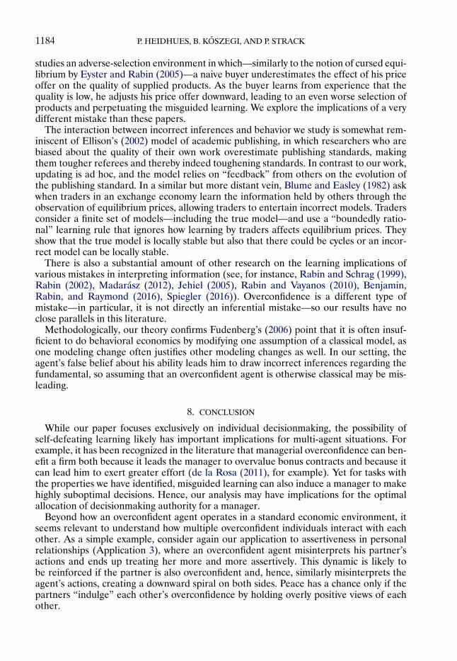
1184 P. HEIDHUES, B. KOSZEGI, AND P. STRACK
studies an adverse-selection environment in which—similarly to the notion of cursed equi-librium by Eyster and Rabin (2005)—a naive buyer underestimates the effect of his priceoffer on the quality of supplied products. As the buyer learns from experience that thequality is low, he adjusts his price offer downward, leading to an even worse selection ofproducts and perpetuating the misguided learning. We explore the implications of a verydifferent mistake than these papers.
The interaction between incorrect inferences and behavior we study is somewhat rem-iniscent of Ellison’s (2002) model of academic publishing, in which researchers who arebiased about the quality of their own work overestimate publishing standards, makingthem tougher referees and thereby indeed toughening standards. In contrast to our work,updating is ad hoc, and the model relies on “feedback” from others on the evolution ofthe publishing standard. In a similar but more distant vein, Blume and Easley (1982) askwhen traders in an exchange economy learn the information held by others through theobservation of equilibrium prices, allowing traders to entertain incorrect models. Tradersconsider a finite set of models—including the true model—and use a “boundedly ratio-nal” learning rule that ignores how learning by traders affects equilibrium prices. Theyshow that the true model is locally stable but also that there could be cycles or an incor-rect model can be locally stable.
There is also a substantial amount of other research on the learning implications ofvarious mistakes in interpreting information (see, for instance, Rabin and Schrag (1999),Rabin (2002), Madarász (2012), Jehiel (2005), Rabin and Vayanos (2010), Benjamin,Rabin, and Raymond (2016), Spiegler (2016)). Overconfidence is a different type ofmistake—in particular, it is not directly an inferential mistake—so our results have noclose parallels in this literature.
Methodologically, our theory confirms Fudenberg’s (2006) point that it is often insuf-ficient to do behavioral economics by modifying one assumption of a classical model, asone modeling change often justifies other modeling changes as well. In our setting, theagent’s false belief about his ability leads him to draw incorrect inferences regarding thefundamental, so assuming that an overconfident agent is otherwise classical may be mis-leading.
8. CONCLUSION
While our paper focuses exclusively on individual decisionmaking, the possibility ofself-defeating learning likely has important implications for multi-agent situations. Forexample, it has been recognized in the literature that managerial overconfidence can ben-efit a firm both because it leads the manager to overvalue bonus contracts and because itcan lead him to exert greater effort (de la Rosa (2011), for example). Yet for tasks withthe properties we have identified, misguided learning can also induce a manager to makehighly suboptimal decisions. Hence, our analysis may have implications for the optimalallocation of decisionmaking authority for a manager.
Beyond how an overconfident agent operates in a standard economic environment, itseems relevant to understand how multiple overconfident individuals interact with eachother. As a simple example, consider again our application to assertiveness in personalrelationships (Application 3), where an overconfident agent misinterprets his partner’sactions and ends up treating her more and more assertively. This dynamic is likely tobe reinforced if the partner is also overconfident and, hence, similarly misinterprets theagent’s actions, creating a downward spiral on both sides. Peace has a chance only if thepartners “indulge” each other’s overconfidence by holding overly positive views of eachother.

UNREALISTIC EXPECTATIONS AND MISGUIDED LEARNING 1185
A completely different issue is that different individuals may have different interpreta-tions as to what explains unexpectedly low performance. For instance, a Democrat mayinterpret poor health outcomes as indicating problems with the private market, whereasa Republican may think that the culprit is government intervention. In the formalism ofour model, one side believes that output is increasing in φ, while the other side believesthat output is decreasing in φ. Similarly to Dixit and Weibull’s (2007) model of politicalpolarization, decisionmakers with such opposing theories may prefer to adjust policies indifferent directions. Our model highlights that unrealistically high expectations regardingoutcomes can play an important role in political polarization. Furthermore, our modelmakes predictions on how the two sides interpret each other’s actions. It may be thecase, for instance, that if a Republican has the power to make decisions, he engages inself-defeating learning as our model predicts, with a Democrat looking on in dismay andthinking that—if only he had the power—a small adjustment in the opposite directionwould have been sufficient. If the Democrat gets power, he adjusts a little in the oppositedirection, initially improving performance, but then he engages in self-defeating learn-ing of his own. Frequent changes in power therefore help keep self-defeating learningin check. Meanwhile, an independent who also has unrealistic expectations but is unsureabout which side’s theory of the world is correct always tends to move his theory towardthe theory of the party in opposition, as that party’s theory is better at explaining currentobservations.
APPENDIX: PROOFS
A.1. Auxiliary Results
This preliminary section introduces useful notation for the main proofs, shows thatexpected output and its derivative with respect to et are well defined, that output has anintuitive influence on subjective beliefs, and applies a well known result from Berk (1966)on the convergence of subjective beliefs with fixed actions to our setting.
We say that a probability density function f has decreasing tails if there is a εc > 0 suchthat ε > ε′ > εc or ε < ε′ <−εc implies f (ε)≤ f (ε′).
LEMMA 1: Since f is log concave, it has decreasing tails.
PROOF: Log-concavity of f implies that (f ′/f ) is decreasing. Because the density hasto integrate to 1, the fact that (f ′/f ) is decreasing implies that there exists some εc suchthat both for all ε > εc , one has f ′ < 0, and for all ε <−εc , one has f ′ > 0. Therefore, fhas decreasing tails. Q.E.D.
LEMMA 2: Suppose that f is bounded and has decreasing tails, and that πt−1 has positivedensity everywhere. Then πt has positive density everywhere, and for any et� qt and any ν > 0,there is a φht > 0 such that if φ>φ′ >φht or φ<φ′ <−φht , then
πt(φ)
πt(φ′) < (1 + ν) πt−1(φ)
πt−1
(φ′) �
PROOF: By Bayes’ rule,
πt(φ)= f(qt −Q(et� a�φ)
)πt−1(φ)∫
f(qt −Q(et� a� s)
)πt−1(s)ds
�

1186 P. HEIDHUES, B. KOSZEGI, AND P. STRACK
The numerator is clearly positive, and since f is bounded, the denominator is positive andfinite, so πt(φ) is positive.
We show the claim of the lemma on the positive tail; the proof is analogous for thenegative tail. Furthermore, the claim is obvious if φ is finite, so we suppose that φ isinfinite. Notice that
πt(φ)
πt(φ′) = f
(qt −Q(et� a�φ)
)f(qt −Q
(et� a�φ
′)) · πt−1(φ)
πt−1
(φ′) �
Now we consider two cases. First, suppose that limφ→∞Q(et� a�φ) = q < ∞. Thenlimφ→∞ f (qt − Q(et� a�φ)) = f (qt − q). This implies that there is a φht such that ifφ�φ′ >φht , then
f(qt −Q(et� a�φ)
)f(qt −Q
(et� a�φ
′)) < 1 + ν�
completing the proof for this case.Alternatively, suppose that limφ→∞Q(et� a�φ) = ∞. Then there is a φht such that if
φ > φ′ > φht , then qt − Q(et� a�φ) < qt − Q(et� a�φ′) < −εc . Hence, f (qt − Q(et� a�
φ))≤ f (qt −Q(et� a�φ′)), again completing the proof. Q.E.D.
For the following result, we first note that the existence of all moments (|E[φk]| <∞for all k) of π0 implies the existence of all absolute moments (E[|φ|k] <∞ for all k).Observe that for k even, |E[φk]| = E[|φ|k] and, thus, |E[φk]|<∞ ⇒ E[|φ|k]<∞. For kodd, we have that
|φ|k ≤ max{1� |φ|k}≤ max
{1� |φ|k+1
}≤ 1 + |φ|k+1 = 1 +φk+1�
Thus, E[|φ|k] ≤ 1+E[φk+1] = 1+|E[φk+1]|<∞ and the existence of the k+1th momentimplies the existence of the kth absolute moment.
LEMMA 3: The posterior belief admits a density πt and all its absolute moments are finiteafter any history.
PROOF: We are going to show the result by induction over t. First, the prior π0 has apositive density by assumption, and since it has finite moments, by the argument aboveits absolute moments are also finite. We will show that if the posterior at time t − 1 has apositive density and all its moments are finite then the posterior at time t is well definedand all its moments are finite.
By Lemmata 1 and 2 the posterior density πt is well defined. To show that all momentsexist, we need to verify that for any k≥ 1 the absolute moment
χk�t =∫ +∞
−∞πt(ψ)|ψ|k dψ
is finite. To show this, first note that Lemma 2 implies that for every ν > 0, there exists aφht such that if φ>φ′ >φht or φ<φ′ <−φht , then
πt(φ)
πt−1(φ)< (1 + ν) πt
(φ′)
πt−1
(φ′) �

UNREALISTIC EXPECTATIONS AND MISGUIDED LEARNING 1187
It follows from this that
χk�t =∫ +∞
−∞πt(ψ)|ψ|k dψ=
∫ +φht
−φhtπt(ψ)|ψ|k dψ+
∫(−∞�−φht )∪(φht �∞)
πt(ψ)|ψ|k dψ
≤ max{1�∣∣φht ∣∣k}+
∫(−∞�−φht )∪(φht �∞)
πt−1(ψ)πt(ψ)
πt−1(ψ)|ψ|k dψ
≤ max{1�∣∣φht ∣∣k}+
∫(−∞�−φht )∪(φht �∞)
πt−1(ψ)(1 + ν) πt(φht
)πt−1
(φht
) |ψ|k dψ
≤ max{1�∣∣φht ∣∣k}+ (1 + ν) πt
(φht
)πt−1
(φht
) ∫ +∞
−∞πt−1(ψ)|ψ|k dψ
= max{1�∣∣φht ∣∣k}+ (1 + ν) πt
(φht
)πt−1
(φht
)χk�t−1�
Thus, the kth moment of the posterior in period t is finite if the kth moment of theposterior in period t − 1 is finite. Q.E.D.
Recall that by assumption Q and Qe have polynomial growth, that is, |Q(e�a�φ)| +|Qe(e�a�φ)| ≤ κ|φ|k + b for some κ�k�b > 0.
PROPOSITION 9: The expected payoff is well defined for every action e and ability a afterevery history, and the expected payoff’s derivative with respect to the action is given by
∂
∂e
∫ +∞
−∞Q(e�a�ψ)πt(ψ)dψ=
∫ +∞
−∞Qe(e�a�ψ)πt(ψ)dψ�
PROOF: Polynomial growth implies that the expected payoff is bounded by the kthabsolute moment and, thus, is well defined:∫ ∞
−∞
∣∣Q(e�a�ψ)∣∣πt(ψ)dψ≤∫ ∞
−∞
(b+ κ|φ|k)πt(ψ)dψ= b+ κχk�t �
Note that |Qe(e�a�φ)| ≤ κ|φ|k + b and as |φ|k is integrable with respect to πt , the domi-nated convergence theorem implies that
∂
∂e
∫ +∞
−∞Q(e�a�ψ)πt(ψ)dψ=
∫ +∞
−∞Qe(e�a�ψ)πt(ψ)dψ� Q.E.D.
Let L(x) = E[log f (x + εt)], where the expectation is taken with respect to εt . Notethat as ε1� ε2� � � � are i.i.d., this expectation is independent of t. Our first result shows thatthe log-concavity of f implies that L is single-peaked, with its peak at zero. Let g(x) =∂∂x(log f (x)) and let |κf | denote the bound on the absolute value of g′, that is, |κf |> |g′|.
LEMMA 4: The function L(x) is well defined for all x ∈ R. Furthermore,(i) L(·) is strictly concave,
(ii) L′(x) > 0 for x < 0 and L′(x) < 0 for x > 0.

1188 P. HEIDHUES, B. KOSZEGI, AND P. STRACK
PROOF: As the distribution of ε is log concave, it has finite variance σ2 = E[|εt |2] (see,for example, Proposition 5.2 in Saumard and Wellner (2014)). Our bounded log-concavityassumption on f implies that
∣∣log(f (x+ ε))∣∣= ∣∣∣∣log
(f (x)
)+∫ x+ε
x
g(z)dz∣∣∣∣
=∣∣∣∣log
(f (x)
)+ εg(x)+∫ x+ε
x
∫ z
x
g′(y)dy dz∣∣∣∣
≤ ∣∣log(f (x)
)∣∣+ |ε|∣∣g(x)∣∣+ |ε|2|κf |
2�
It thus follows that ∣∣L(x)∣∣= ∣∣E[log f (x+ εt)]∣∣≤ E
[∣∣log f (x+ εt)∣∣]
≤ ∣∣log(f (x)
)∣∣+E[|εt |]∣∣g(x)∣∣+E
[|εt |2] |κf |
2
≤ ∣∣log(f (x)
)∣∣+ σ∣∣g(x)∣∣+ σ2|κf |
2�
where we used in the last step that by Jensen’s inequality E[|ε|] ≤ √E[|ε|2] = σ . Thus,
L(x) is well defined for every x.As our log-concavity assumption implies that |g| and |g′| are bounded by an integrable
function, majorized convergence yields that the derivatives of L(·) are given by
L′(x)=∫R
g(x+ ε)f (ε)dε�
L′′(x)=∫R
g′(x+ ε)f (ε)dε ∈ [κf �0)�
Since g′ < 0, L is strictly concave. To see that the peak is at zero, note that
L(x)−L(0)= E[log f (x+ εt)− log f (εt)
]= −E
[log
(f (εt)
f (x+ εt))]�
The right-hand side equals minus the Kullback–Leibler divergence. By Gibb’s inequalitythe Kullback–Leibler divergence is larger or equal to zero, holding with equality if andonly if both densities coincide almost everywhere (a.e.). Hence, the right-hand side isminimized at x = 0, so that L(·) is maximized at x = 0. Finally, as L is strictly concaveand maximized at 0, it follows that L′(0) = 0, and L′(x) is thus positive for x < 0 andnegative for x > 0. Q.E.D.
Denote by �0 : R → R the subjective prior log-likelihood of the agent. By Bayes’ rulethe agent’s subjective log-likelihood �t :R → R assigned to the state φ in period t is givenby
�t(φ)=t∑s=1
log f(qs −Q(es� a�φ)
)+ �0(φ)� (5)

UNREALISTIC EXPECTATIONS AND MISGUIDED LEARNING 1189
The density function πt :R → R+ of the agent’s subjective belief in period t equals
πt(φ)= e�t (φ)∫ ∞
−∞e�t (z) dz
�
Denote by Pt[·] = P[· | q1� � � � � qt] the agent’s subjective probability measure over statesconditional on the outputs q1� � � � � qt and denote by �t : R → [0�1] the cumulative distri-bution function (cdf) of the agent’s subjective belief
�t(z)= Pt[Φ≤ z] =∫ z
−∞πt(φ)dφ�
We sometimes write �t(φ;q) and πt(φ;q) if we want to highlight the dependence ofthe agent’s belief on the outputs q1� � � � � qt observed in previous periods.
DEFINITION 2—Monotone Likelihood Ratio Property: A distribution with density π :R → R+ is greater than a distribution with density π ′ : R → R+ in the sense of monotonelikelihood ratio π ′ ≤MLR π if and only if for all states φ′ ≤φ,
π ′(φ)π(φ)
≤ π ′(φ′)π(φ′) � (MLRP)
The next lemma shows that higher observed output qt in any period t leads to a higherposterior belief in the sense of monotone likelihood ratios (MLR).
LEMMA 5—Beliefs are Monotone in Output: If q′s ≤ qs for all s ≤ t, then πt(·;q′)≤MLR
πt(·;q).PROOF: Condition (MLRP) is equivalent to
0 ≤ log[πt(φ;q)πt(φ′;q)
]− log
[πt(φ;q′)
πt(φ′;q′)
]= [�t(φ;q)− �t
(φ′;q)]− [
�t(φ;q′)− �t
(φ′;q′)]�
Hence, it suffices to show that for all s ≤ t,∂2�t(φ;q)∂qs∂φ
≥ 0�
Taking the derivative of the log-likelihood given in Equation (5) yields that for s ≤ t,∂2�t(φ;q)∂qs∂φ
= −g′(qs −Q(es� a�φ))Qφ(es� a�φ)�
As g′ < 0 and Qφ > 0, the result follows. Q.E.D.
Our next result shows that beliefs converge when the agent takes the same action inevery period. As in this case the outputs are independent, the result follows immediatelyfrom the characterization of long-run beliefs with i.i.d. signals in Berk (1966).

1190 P. HEIDHUES, B. KOSZEGI, AND P. STRACK
LEMMA 6—Berk (1966): Suppose that the agent takes a fixed action e in all periods andthere exists a state φe∞ ∈ (φ�φ) that satisfies
Q(e�A�Φ)=Q(e� a�φe∞)� (6)
Then the agent’s belief almost surely (a.s.) converges and concentrates on the unique stateφe∞.
PROOF: For fixed actions, outputs q1� q2� � � � are i.i.d. random variables. The expecta-tion of an outside observer of the log-likelihood that the agent assigns to the state φ afterobserving a single signal qt is given by
E[log f
(qt −Q(e� a�φ)
)]= E[log f
(Q(e�A�Φ)−Q(e� a�φ)+ εt
)]=L
(Q(e�A�Φ)−Q(e� a�φ))� (7)
By the main theorem in Berk (1966, p. 54), the agent’s subjective belief concentrateson the set of maximizers of (7). By Lemma 4, L(·) is uniquely maximized at zero and,hence, (7) is maximized whenever (6) is satisfied. By assumption there exists such a pointand since Qφ > 0 it is unique. Hence, the agent’s subjective belief converges to a Diracmeasure on that point. Q.E.D.
Let us denote a Dirac measure on the state φ by δφ.
LEMMA 7: The set (e�π) is a pure-strategy Berk–Nash equilibrium if and only if π is astable belief δφ and e= e∗(φ).
PROOF: For a given state φ′ and action e, the Kullback–Leibler divergence betweenthe true distribution of signals and the distribution that the agent expects is given by
E
[log
f (εt)
f(Q(e�A�Φ)−Q(e� a�φ′)+ εt
)]=L(0)−L(Q(e�A�Φ)−Q(e� a�φ′))�
By the definition of Berk–Nash equilibrium, the agent assigns positive probability only tostates that minimize the Kullback–Leibler divergence. Since, by Lemma 4, L(·) is maxi-mized at 0, it follows that the agent’s belief is a Dirac measure on the state φ that satisfiesQ(e�A�Φ)−Q(e� a�φ)= 0. Because the equilibrium action must be optimal given thisbelief, it follows that (e∗(φ)�δφ) is a pure-strategy Berk–Nash equilibrium if and only ifφ is a stable belief. Q.E.D.
A.2. Main Results
A.2.1. Proving Properties of Limiting Beliefs
We first show that all stable beliefs are in an interval around the true state Φ if Qa andQφ are bounded.
LEMMA 8: Let κa ≥Qa be an upper bound on Qa and let 0< κφ ≤Qφ be a lower boundon Qφ. Any root of � lies in the interval Ia = [Φ− κa
κφ(a−A)�Φ]. Furthermore, �(Φ) < 0
and �(Φ− κaκφ(a−A))≥ 0, so if Ia ⊂ (φ�φ), then � has at least one root in Ia.

UNREALISTIC EXPECTATIONS AND MISGUIDED LEARNING 1191
PROOF: Note that for a=A, the surprise function
�(φ)=Q(e∗(φ)�A�Φ)−Q(e∗(φ)� a�φ
)has a unique root at φ =Φ since Qφ > 0. Furthermore, since Qa > 0 and Qφ > 0, whena > A any root of � must be less than Φ. Now for any φ<Φ,
�(φ)≥ mine
{Q(e�A�Φ)−Q(e� a�φ)}
= mine
{Q(e�A�Φ)−Q(e�A�φ)+Q(e�A�φ)−Q(e� a�φ)}
≥ κφ(Φ−φ)− κa(a−A)�
Therefore, any root of � must lie in the interval Ia = [Φ− κaκφ(a−A)�Φ]. Furthermore,
since A< a, we have that �(Φ) < 0, and by the above inequality, �(Φ− κaκφ(a−A))≥ 0.
It thus follows from the continuity of � that � has at least one root in Ia. Q.E.D.
PROOF OF PROPOSITION 1: Part (i). We first show that for a−A sufficiently small, �can have at most one root. Since e∗(φ) is implicitly defined through Qe(e
∗(φ)� a�φ)= 0and Q is twice continuously differentiable with Qee < 0, e∗(φ) is a continuous functionof φ and a. By the implicit function theorem, e∗′
(φ) = −Qeφ/Qee and, hence, is also acontinuous function of φ and a. Thus,
�′(φ)=Qe
(e∗(φ)�A�Φ
)(e∗)′(φ)−Qφ
(e∗(φ)� a�φ
)is a continuous function of φ and a. Since for a=A and φ=Φ,
�′(φ)|φ=Φ�a=A = −Qφ
(e∗(φ)�A�Φ
)< 0�
continuity of �′(φ) implies that there exists a pair ηA�ηΦ > 0 such that for all a ∈ [A�A+ηA) and φ ∈ (Φ − ηΦ�Φ], one has �′(φ) < 0. Thus, for any a ≥ A that satisfies a <A+ min{ηA�ηΦ + κφ
κa}, one has that �′(φ) < 0 over the relevant interval Ia. By Lemma 8,
all roots of � lie in Ia and, thus, for all such a, � has a unique root. Furthermore, fora−A small enough, Ia ⊂ (φ�φ) and, hence, by Lemma 8, � crosses zero in (φ�φ). Weconclude that � has a unique root if overconfidence (a−A) is sufficiently small.
Part (ii). When Q takes the form in Example 1, then e∗(φ)=φ and
�(φ)= −(a−A)+ (Φ−φ)−L(Φ−φ)�Since L′(x) < 1, �′(φ) < 0 and, hence, � has at most one root. Finally, as (φ�φ)= R, wehave that Ia ⊂ (φ�φ) and, hence, there exists a stable belief by Lemma 8.
Part (iii). SinceQa > 0 andQφ > 0, when a > A any root of �must be less thanΦ. Nowφ is a root of � if and only if (A+ e∗(φ))Φ= (a+ e∗(φ))φ, or
e∗(φ)= −A+ (a−A)φ/(Φ−φ)� (8)
The right-hand side of this equation is increasing and convex over the interval (0�Φ),negative at φ= 0, and approaches ∞ as φ approaches Φ.

1192 P. HEIDHUES, B. KOSZEGI, AND P. STRACK
Furthermore, for e∗(φ) to be optimal given φ, we must have c′(e∗(φ)) = φ. This im-plies that e∗′(φ)= 1/c′′(e∗(φ)), so that if c′′′(e)≥ 0, then e∗(φ) is concave. Furthermoree∗(0) = 0 and e∗(Φ) is finite, so that it equals the right-hand-side of (8) at exactly onepoint. Q.E.D.
PROOF OF PROPOSITION 2: By Lemma 6, if, for any fixed action e the unique solutionφe∞ to
0 =Q(e�A�Φ)−Q(e� a�φe∞)satisfies φe∞ ∈ (φ�φ), beliefs converge to a Dirac measure on φe∞. Since a > A andQa�Qφ > 0, we have φe∞ < Φ. Let φ∞ be the state corresponding to the unique stablebelief. Since φ∞ ∈ (φ�φ) and φe∞ <Φ<φ, we have that φ∞ ≤φe∞ implies φe∞ ∈ (φ�φ).
By definition of φ∞,
�(φ∞)=Q(e(φ∞)�A�Φ)−Q(e(φ∞)� a�φ∞
)= 0�
Since Qa > 0 and Qφ > 0, when a > A one has φ∞ <Φ. Furthermore, when the agent’sbelief are a Dirac measure on φ, he chooses the myopically optimal action that satisfies
Qe
(e(φ)� a�φ
)= 0�
By the implicit function theorem, e∗′(φ)= −Qeφ/Qee > 0. Hence, e(φ∞) < e∗(Φ).
Since Qeφ > 0 and, by Assumption 1, Qae ≤ 0, the derivative
∂
∂e
[Q(e�A�Φ)−Q(e� a�φe∞)]= −
∫ a
A
Qae(e�a�Φ)da+∫ Φ
φe∞Qφe(e� a�φ)dφ> 0�
Because Q(e�A�Φ)−Q(e� a�φe∞)= 0 and e(φ∞) < e∗(Φ)≤ e, therefore,
Q(e(φ∞)�A�Φ
)−Q(e(φ∞)� a�φe∞)< 0 =Q(e(φ∞)�A�Φ
)−Q(e(φ∞)� a�φ∞)�
Since Qφ > 0, it follows that φ∞ <φe∞. Q.E.D.
PROOF OF PROPOSITION 3: Since Qa > 0, Qφ > 0, and a > A, the surprise function�i is negative for all φ ≥ Φ and, hence, has a negative slope at its unique root φ∞�i.Furthermore, when the agent’s belief are a Dirac measure onφ, he chooses the myopicallyoptimal action that satisfies
Qe
(e(φ)� a�φ
)= 0�
By the implicit function theorem, e∗′(φ) = −Qeφ/Qee > 0 and e∗′
(a) = −Qea/Qee ≤ 0.Since φ∞�i < Φ and a > A, the agent chooses a suboptimally low stable action. Be-cause �i(φ) = Ri(A�Φ) − Ri(a�φ) − Li(e
∗(a�φ)�A�Φ), �1 > �2 pointwise at all butthe optimal action, the fact that the agent chooses some suboptimal action implies thatφ∞�1 >φ∞�2. Q.E.D.
LEMMA 9—Monotonicity of Stable Beliefs: The subjective φ∞ is increasing and contin-uous in the true state Φ.

UNREALISTIC EXPECTATIONS AND MISGUIDED LEARNING 1193
PROOF: The stable state φ∞ is defined as the unique solution φ to
Q(e∗(φ)�A�Φ
)−Q(e∗(φ)� a�φ)= 0� (9)
Now fix a φ∞ for a given Φ. Slightly increase Φ to Φ′ > Φ. Then the left-hand side in-creases, while the right-hand side remains unchanged, so
Q(e∗(φ∞)�A�Φ′)−Q(e∗(φ∞)� a�φ∞
)> 0�
We know that for φ>Φ′, Q(e∗(φ)�A�Φ) <Q(e∗(φ)� a�φ). So
Q(e∗(φ)�A�Φ′)−Q(e∗(φ)� a�φ
)< 0 for φ>Φ′�
Q(e∗(φ∞)�A�Φ′)−Q(e∗(φ∞)� a�φ∞
)> 0 for φ>φ∞�
By the continuity of Q and e∗, there must be a new solution to the equation
Q(e∗(φ)�A�Φ′)−Q(e∗(φ)� a�φ
)= 0
that satisfies φ ∈ (φ∞�Φ′]. Since the stable belief is unique, this implies that the stablebelief associated with the state Φ′ is greater than the stable belief associated with thestate Φ.
The continuity of the stable belief in the true state follows from the differentiability ofQ by applying the implicit function theorem to (9). Q.E.D.
PROOF OF PROPOSITION 4: Consider first the overconfident agent. Since u1 > u, theagent chooses the task in the first period. Because by Lemma 9 the long-run belief of theagent is increasing and continuous in the true state and, in addition, Q(e(φ∞)� a� φ∞)) <u, there exists a critical state Φ > Φ such that the agent eventually abandons the taskwhenever the realized state Φ < Φ. By Chebyshev’s inequality, the probability that thestate is in a range where the agent does not eventually abandon the task is bounded bythe prior variance σ2
0 :
P
[|Φ− Φ| ≥ 1
2|Φ− Φ|
]≤ 2σ2
0
(Φ− Φ)2�
As σ20 → 0, the probability that Φ< Φ approaches 1. Therefore, as σ2
0 → 0, the probabil-ity that the agent eventually abandons the task approaches 1.
Now we turn to the rational agent. Since maxe Q(e�A� Φ) > u, Lipschitz continuity ofQ in the state implies that for a sufficiently small prior variance σ2
0 , the agent choosesthe task in the first period. Now we prove the following statement: if the agent choosesthe task in the first period, then the probability that he ever takes the outside option isbounded by σ2
0 times a constant, and hence approaches 0 as σ20 → 0.
Without loss of generality, let u= 0 to simplify notation (otherwise normalize the out-put function by subtracting u from Q). Let
mt = Et
[Q(e1�A�Φ)
]−E1
[Q(e1�A�Φ)
]� (10)
Since maxe Q(e�A� Φ) > u = 0, it follows from the continuity of Q that for sufficientlysmall σ0, it holds that E1[Q(e1�A�Φ)]> 0, that is, the agent finds it initially optimal not

1194 P. HEIDHUES, B. KOSZEGI, AND P. STRACK
to take the outside option. Note that mt is by construction a martingale. As the agentpicks an optimal action, a lower bound on the agent’s payoff is given by the expectedpayoff implied from taking the initial action e1 forever:
maxe
Et
[Q(e�A�Φ)
]≥ Et
[Q(e1�A�Φ)
]=mt +E1
[Q(e1�A�Φ)
]�
Thus, the agent refrains from taking the outside option in period t as long as |mt | is nottoo large:
|mt |< E1
[Q(e1�A�Φ)
] ⇒ 0<mt +E1
[Q(e1�A�Φ)
]≤ maxe
Et
[Q(e�A�Φ)
]�
Hence, an upper bound on the probability that the agent takes the outside option beforeperiod t is given by the probability that the absolute value of the martingale m exceedsu1 = E1[Q(e1�A�Φ)]:
P
[mins≤t
(maxe
Et
[Q(e�A�Φ)
])≤ 0]
≤ P
[maxs≤t
|ms| ≥ u1
]�
Applying the Burkholder–Davis–Gundi inequality to the martingale (mt)t yields thatthere exists a constant κ such that
P
[maxs≤t
|ms| ≥ u0
]≤ κ× (
E[m2t
]−E[m2
1
]︸ ︷︷ ︸=0
)
= κ×E[(Et
[Q(e1�A�Φ)
]−E1
[Q(e1�A�Φ)
])2]= κ×E
[(Et
[Q(e1�A�Φ)−E1
[Q(e1�A�Φ)
]])2]≤ κ×E
[Et
[(Q(e1�A�Φ)−E1
[Q(e1�A�Φ)
])2]]= κ×E
[(Q(e1�A�Φ)−E1
[Q(e1�A�Φ)
])2]�
(11)
where we use Jensen’s inequality in the second inequality and the law of iterated expec-tations in the last equality. To bound the right-hand side, we need to bound the priorvariance associated with the payoff of the initial action. As Q is Lipschitz continuous inφ, we have that the right-hand side of (11) can be bounded by the prior variance
E[(Q(e1�A�Φ)−E1
[Q(e1�A�Φ)
])2]= E[(Q(e1�A�Φ)−E1
[Q(e1�A�Φ)
])2]= E
[(Q(e1�A�Φ)−
∫Q(e1�A�z)π0(z)dz
)2]
= E
[(∫Q(e1�A�Φ)−Q(e1�A�z)π0(z)dz
)2]
≤ κ2φE
[(∫(Φ− z)π0(z)dz
)2]
≤ κ2φE
[∫(Φ− z)2π0(z)dz
]= κ2
φσ20 �

UNREALISTIC EXPECTATIONS AND MISGUIDED LEARNING 1195
where the last inequality follows from Jensen’s inequality. Hence, there exists some con-stant κ′ such that
P
[sups≤t
|ms −m0| ≥ k]
≤ κ′ × σ20 �
Thus, the probability that the agent takes the outside option before period t is boundedby the prior variance times a constant
P
[mins≤t
(maxe
Es
[Q(e�A�Φ)
])≤ 0]
≤ κ′ × σ20 �
Because the right-hand side is independent of t, the limit t to infinity of the above equa-tion is well defined. Using independence of t, existence of the limit, and dominated con-vergence, we conclude that
limt→∞
P
[mins≤t
(maxe
Es
[Q(e�A�Φ)
])≤ 0]
= P
[limt→∞
mins≤t
(maxe
Es
[Q(e�A�Φ)
])≤ 0]
= P
[mint
(maxe
Et
[Q(e�A�Φ)
])≤ 0]
≤ κ′ × σ20 � Q.E.D.
PROOF OF PROPOSITION 5: (i) ⇒ (ii). Denote by φ(A� a�Φ) the state correspondingto the unique stable belief when perceived ability equals a, true ability equals A, and thetrue state equals Φ. Denote by e∗(a�φ) the optimal action when the ability equals a andthe state equals φ.
Since the action is objectively optimal for the state Φ as well as subjectively optimalwhen the agent holds beliefs φ(A� a�Φ), we have
e∗(A�Φ)= arg maxeQ(e�A�Φ)= arg max
eQ(e� a� φ(A� a�Φ)
)= e∗(a� φ(A� a�Φ)) (12)
for allA, a,Φ. Furthermore, by the definition of a stable belief, the agent gets no surprise:
Q(e∗(A�Φ)�A�Φ
)=Q(e∗(A�Φ)� a� φ(A� a�Φ))
(13)
for all A� a�Φ.We establish some properties of e∗(a�φ). First, we know that e∗
φ(a�φ) > 0. Second,we show that e∗
a(a�φ) > 0 (recall that we do not assume Qea ≥ 0 in Proposition 5). To-tally differentiating Equation (13) with respect to a and using that Qa > 0, we get thatφa(a� a�φ) < 0. Furthermore, by Equation (12) we have e∗(a�φ) = e∗(a� φ(a� a�φ)).Totally differentiating this equality with respect to a gives that e∗
a(a� φa(a� a�φ)) =−e∗
φ(a� φa(a� a�φ))φa(a� a�φ) > 0. Setting a = a and using that φ(a�a�φ) = φ estab-lishes our claim that e∗
a(a�φ) > 0.Given these properties, we can define S(a�φ) = e∗(a�φ), and this function satisfies
Sa�Sφ > 0. Furthermore, using again that e∗(a�φ) = e∗(a� φ(a� a�φ)), note that forany a� a�φ, the unique φ′ satisfying S(a�φ) = S(a�φ′) is φ′ = φ(a� a�φ). Now we de-fine V (e�S) = S − L(|e − S|), where L(·) is any strictly increasing function satisfyingL′(x) < 1 everywhere. By construction, VS > 0, and because S(a� φ(A� a�Φ))= S(A�Φ),

1196 P. HEIDHUES, B. KOSZEGI, AND P. STRACK
�(φ(A� a�Φ)) = 0. Thus, the Dirac measure on φ(A� a�Φ) is the stable belief andS(a� φ(A� a�Φ))= e∗(a� φ(A� a�Φ))= e∗(A�Φ) is the stable action.
(ii) ⇒ (i). Because VS�Sa� Sφ > 0, for any action e there is a unique φ such thatV (e�S(A�Φ))= V (e�S(a� φ)). At this φ, �(φ)= 0, and, hence, δφ = δφ∞ is a stable be-lief. Hence the stable action e∗(φ∞) of the agent satisfies Ve(e∗(φ∞)� S(a�φ∞))= 0, andsince Ve(e�S(a�φ∞))= Ve(e�S(A�Φ)), the stable action is optimal if the output functiontakes the form V (e�S(a�φ)). Q.E.D.
A.2.2. Belief Concentration in the Myopic Case
We now prove Theorem 1.Step 1: In the Long Run the Expected Change Approximates the Actual Change in Beliefs.
To characterize the long-run behavior of the agent’s beliefs, we show that the change in hisbeliefs in the long run can be approximated well by the expected change. To establish this,we use the fact that the log-likelihood function is the average of the log-likelihoods of therealized outputs. As the log-likelihood is an average of nonidentical and nonindependentrandom variables, however, we need to generalize existing versions of the law of largenumbers to non-i.i.d. random variables. To do so, we use the fact that a square-integrablemartingale divided by its quadratic variation converges to zero whenever the quadraticvariation goes to infinity.
The following proposition states a law of large numbers like result for square-integrableMartingales with bounded quadratic variation. Recall the definition of the quadratic vari-ation of a martingale (yt)t as
[y]t =t−1∑s=1
E[(ys+1 − ys)2 |Fs
]� (14)
where Fs denotes filtration of an outside observer who knows the state at time s, that is,the expectation is taken with respect to all information available at time s. For brevity, werefer to the martingale (yt)t as martingale y .
PROPOSITION 10—Law of Large Numbers: Let (yt)t be a martingale that satisfies a.s.[y]t ≤ vt for some constant v≥ 0. We have that a.s.
limt→∞
yt
t= 0�
PROOF: We first show that y is square integrable. By the law of iterated expectations,we have that
E[y2t
]= E
[y2
1 +t−1∑s=1
y2s+1 − y2
s
]= y2
1 +E
[t−1∑s=1
E[y2s+1 − y2
s |Fs
]]
= y21 +E
[t−1∑s=1
E[(ys+1 − ys)2 |Fs
]]= y21 +E
[[y]t]≤ y21 + vt�
Consequently, the martingale y is square integrable.

UNREALISTIC EXPECTATIONS AND MISGUIDED LEARNING 1197
In the next step we show that limt→∞ytt
= 0 almost surely. If the limit of the quadraticvariation [y]∞ = limt→∞[y]t exists, the martingale y converges almost surely (Theo-rem 12.13 in Williams (1991)), and hence limt→∞
ytt
= 0. Hence, from now on we con-sider the remaining histories for which the quadratic variation does not converge. We canrewrite the average value of the martingale y as
yt
t= yt
[y]t · [y]tt�
Because the square quadratic variation is monotone increasing by definition, it must goto infinity after those histories. Furthermore (as argued, for example, in Section 12.14in Williams (1991)), for any square-integrable martingale and any history for whichlimt→∞[y]t = ∞, one has that almost surely limt→∞
yt[y]t = 0. Since 0 ≤ [y]t ≤ vt, it follows
that lim supt→∞ | ytt| ≤ v · lim supt→∞ | yt[y]t | = 0 almost surely. Since lim supt→∞ | yt
t| = 0 a.s.,
limt→∞ytt
= 0 a.s. Q.E.D.
To apply the result of Proposition 10, we will, for every fixed beliefφ, consider the Doobdecomposition (Section 12.11 in Williams (1991)) of the derivative of the log-likelihoodprocess into a martingale (yt(φ))t and a previsible process (zt(φ))t , henceforth y(φ) andz(φ).
Let mt(φ) :=Q(et�A�Φ)−Q(et� a�φ). We define xt(φ) as
xt(φ)= −(g(mt(φ)+ εt)−E
[g(mt(φ)+ εt
) |Ft
])Qφ(et� a�φ)
= −(g(mt(φ)+ εt)−E
[g(mt(φ)+ εt
) | et])Qφ(et� a�φ)
= −(g(mt(φ)+ εt)−L′(mt(φ)
))Qφ(et� a�φ)�
(15)
where the second equality uses the fact that an outside observer who knows the true stateneeds only to condition on the current action et to calculate the expected surprise in thenext period. Furthermore, we define yt(φ)=∑t
s=1 xs(φ) and zt(φ) as
zt(φ)= −∑s≤t
L′(ms(φ))Qφ(es� a�φ)�
LEMMA 10: For every φ, the processes (y(φ)� z(φ)) have the properties(i) �′
t(φ)= �′0(φ)+ yt(φ)+ zt(φ),
(ii) |xt(φ)| ≤ κφ|κf |(|εt | + σ),(iii) yt(φ) is a martingale with [y(φ)]t ≤ t3(κφ|κf |σ)2.
PROOF: Part (i) follows immediately from the definition. Furthermore, by constructionE[xt(φ)|Ft] = E[xt(φ) | et] = 0 and, hence, y is a martingale. Using the bound on theabsolute value of the derivative of g, |κf |, part (ii) follows since∣∣xt(φ)∣∣= ∣∣g(mt(φ)+ εt
)−E[g(mt(φ)+ εt
) | et]∣∣Qφ(et� a�φ)
= ∣∣[g(mt(φ)+ εt)− g(mt(φ)
)]−E[g(mt(φ)+ εt
)− g(mt(φ)) | et
]∣∣Qφ(et� a�φ)
≤ κφ∣∣[g(mt(φ)+ εt
)− g(mt(φ))]∣∣+ κφ∣∣E[g(mt(φ)+ εt
)− g(mt(φ)) | et
]∣∣≤ κφ|κf ||εt | + κφ|κf |E
[|εt |]�

1198 P. HEIDHUES, B. KOSZEGI, AND P. STRACK
and by Jensen’s inequality E[|εt |] ≤ √E[|εt |2] = σ . Part (iii) follows from (ii) and the
definition of the quadratic variation (14):
[y(φ)
]t=
t∑s=2
E[x2s |Fs−1
]≤ κ2φ|κf |2
t∑s=2
E[(|εs| + σ)2]
= κ2φ|κf |2
{t∑s=2
E[|εs|2
]+ σ2 +E[|εs|]σ
}≤ 3κ2
φ|κf |2σ2t�Q.E.D.
An immediate corollary from the law of large numbers given in Proposition 10 andLemma 10(iii) is that for every φ, the average of yt(φ) converges to zero almost surely,that is,
limt→∞
yt(φ)
t= 0�
We next want to show that this convergence is uniform in φ.Let φ∞ be the largest number such that the agent almost always convinces himself
eventually that the state Φ is greater than φ∞ and let φ∞ be the smallest number suchthat the agent is eventually convinced that the state is below φ∞, that is,
φ∞ = sup{φ′ : lim
t→∞�t
(φ′)= 0 almost surely
}�
φ∞ = inf{φ′ : lim
t→∞�t
(φ′)= 1 almost surely
}�
DEFINITION 3—Uniform Stochastic Convergence: The sequence (Gt(·))t convergesuniformly over [φ∞�φ∞] stochastically to zero if and only if
limt→∞
supφ∈[φ∞�φ∞]
∣∣Gt(φ)∣∣= 0 a.s. (U-SCON)
For deterministic sequences of real-valued function, Ascoli’s theorem states that point-wise convergence implies uniform convergence if and only if the functions are equicontin-uous. Despite the fact that our sequence of real-valued functions is not equicontinuous forevery realization, we use a stochastic analogue—strong stochastic equicontinuity (SSE) asdefined on p. 245 in Andrews (1992)—to establish uniform convergence below.
DEFINITION 4—Strong Stochastic Equicontinuity: Let G∗t (φ) = sups≥t |Gs(φ)|. A se-
quence (Gt(·))t is strongly stochastic equicontinuous if and only if:(i) G∗
1(φ) <∞ for all φ ∈ [φ∞�φ∞] a.s.,(ii) for all γ > 0, there exists δ > 0 such that
limt→∞
P
[sup
φ∈[φ∞�φ∞]sup
φ′∈Bδ(φ)
∣∣G∗t (φ)−G∗
t
(φ′)∣∣> γ]< γ�
The usefulness of SSE comes from the fact that almost sure convergence in combinationwith SSE implies (U-SCON).

UNREALISTIC EXPECTATIONS AND MISGUIDED LEARNING 1199
THEOREM 3—Theorem 2(a) in Andrews (1992): IfG satisfies strong stochastic equicon-tinuity andG converges pointwise to zero a.s., thenG converges uniform stochastically to zero.
Our next result argues that the sequence yt (·)t
is strong stochastic equicontinuous andthus converges uniform stochastically to zero.
LEMMA 11: The sequence ( yt (·)t)t converges uniform stochastically to zero.
PROOF: By Lemma 2 in Andrews (1992), strong stochastic equicontinuity of ( yt (·)t)t
follows if the absolute value of the derivative of xt(·) can be uniformly bounded bya random variable Bt for all φ ∈ [φ∞�φ∞] such that supt≥1
1t
∑t
s=1 E[Bs] < ∞ andlimt→∞ 1
t
∑t
s=1(Bs −E[Bs])= 0.From the definition of x in Equation (15) it follows that∣∣x′
t(φ)∣∣= ∣∣(g′(mt(φ)+ εt
)−L′′(mt(φ)))[Qφ(et� a�φ)
]2
− (g(mt(φ)+ εt
)−L′(mt(φ)))Qφφ(et� a�φ)
∣∣≤ ∣∣g′(mt(φ)+ εt
)−L′′(mt(φ))∣∣[Qφ(et� a�φ)
]2
+ ∣∣(g(mt(φ)+ εt)−L′(mt(φ)
))∣∣× ∣∣Qφφ(et� a�φ)∣∣�
Since |g′| ≤ |κf |, one has |L′′(mt(φ))| ≤ |κf |, and by Assumption 2,Qφ ≤ κφ, |Qφφ| ≤ κφφ;using this and substituting xt(φ) yields
∣∣x′t(φ)
∣∣≤ 2|κf |κ2φ + ∣∣xt(φ)∣∣κφφ
κφ≤ 2|κf |κ2
φ + κφφ
κφκφ|κf |
(|εt | + σ)=: Bt�
where the last inequality follows from Lemma 10(ii). As (Bt)t are i.i.d., it follows that
1t
t∑s=1
E[Bs] = E[B0]<∞�
Furthermore, as Bt also has finite variance, the law of large numbers implies limt→∞ 1t×∑t
s=1(Bs −E[Bs])= 0. Q.E.D.
Step 2: No Long-Run Surprises. The next lemma shows that if the agent is always onaverage surprised by the output for some beliefs—i.e.,mt(·) is bounded away from zero—then the absolute value of the derivative of his subjective log-likelihood goes to infinityalmost surely for those beliefs.
Let I denote an interval.
LEMMA 12: (a) If lim inft→∞mt(φ)≥m> 0 for all φ ∈ I, then there exists r > 0 such thata.s.
lim inft→∞
infφ∈I�′t(φ)
t≥ r�
(b) If lim supt→∞mt(φ)≤m< 0 for all φ ∈ I, then there exists r > 0 such that a.s.
lim supt→∞
supφ∈I
�′t(φ)
t≤ −r�

1200 P. HEIDHUES, B. KOSZEGI, AND P. STRACK
PROOF: We show (a); the proof of (b) is analogous. As L′ is decreasing, we have thatfor all φ ∈ I,
L′(mt(φ))≤L′(m)�
We use this fact and that L′(m) < 0 to bound zt(φ) for all φ ∈ I:
zt(φ)= −t∑s=1
L′(mt(φ))Qφ(et� a�φ)
≥t∑s=1
∣∣L′(m)∣∣Qφ(et� a�φ)≥ t · ∣∣L′(m)
∣∣κφ�Define r = |L′(m)|κφ > 0. Using the definition of yt(φ) and zt(φ), r, and the uniformstochastic convergence of yt/t to zero that we established in Lemma 11, respectively, wehave that
lim inft→∞
infφ∈I�′t(φ)
t= lim inf
t→∞infφ∈I�′
0(φ)+ yt(φ)+ zt(φ)t
≥[
lim inft→∞
infφ∈Iyt(φ)
t
]+ r
≥ −[
lim supt→∞
infφ∈I
∣∣yt(φ)∣∣t
]+ r = r�
Q.E.D.
The next lemma argues that if the agent is surprised by the output for an interval ofbeliefs then he will a.s. assign probability 0 to those beliefs in the long run. Intuitively, asby Lemma 12 the absolute value of the derivative of the agent’s subjective likelihood goesto infinity, the absolute value of the derivative of his posterior density goes to infinity.The next lemma shows that this implies that the agent must assign probability 0 to thosebeliefs.
LEMMA 13: (i) If lim inft→∞mt(φ)≥m> 0 for all φ ∈ (l�h)⊂ (φ�φ), then
limt→∞
Pt
[Φ ∈ [l�h)]= 0�
(ii) If lim supt→∞mt(φ)≤m< 0 for all φ ∈ (l�h)⊂ (φ�φ), then
limt→∞
Pt
[Φ ∈ (l�h]]= 0�
PROOF: First consider the case where mt(φ) ≥ m > 0. Lemma 12 implies that therea.s. exists r > 0 such that for sufficiently large t for all y ∈ (l�h),
�′t(y)≥ rt�
Let η= h− l. We have that the probability the agent assigns to state in [l + η/2� l + η]satisfies
Pt
[Φ ∈ [l+η/2� l+η]]=
∫ l+η
l+η/2πt(z)dz =
∫ l+η/2
l
πt(z)πt(z+η/2)πt(z)
dz
=∫ l+η/2
l
πt(z)exp(�t(z+η/2)− �t(z)
)dz

UNREALISTIC EXPECTATIONS AND MISGUIDED LEARNING 1201
=∫ l+η/2
l
πt(z)exp(∫ z+η/2
z
�′t(y)dy
)dz
≥∫ l+η/2
l
πt(z)exp(rtη/2)dz = ertη/2Pt[Φ ∈ [l� l+η/2]]�
As r > 0, we have that the probability assigned to the interval [l� l+η/2] is bounded by aterm that vanishes for t → ∞:
Pt
[Φ ∈ [l� l+η/2]]≤ e−rtη/2
Pt
[Φ ∈ [l+η/2� l+η]]≤ e−rtη/2�
Hence, the agent must assigned zero probability to the interval [l� l+η/2] in the long run.Applying this argument iteratively yields that the agent assigns zero probability to the
interval [l�h). The argument in the case where mt(φ) ≤ m < 0 is completely analo-gous. Q.E.D.
Step 3: Convergence in the Correctly Specified Case. Lemma 13 allows us to argue thatthe agent’s subjective beliefs converge when her model of the world is correctly specified(a=A).
PROPOSITION 11: If a=A, then the agent’s posterior belief converges to a Dirac measureon the true state Φ.
PROOF: Fix an η> 0. We have that for all φ≤Φ−η,
mt(φ)=Q(et�A�Φ)−Q(et� a�φ)≥ ηκφ�Hence, by Lemma 13, we have that a.s. limt→∞�t(Φ− η)= 0 and thus a.s. φ∞ ≥Φ− η.Taking the supremum over η yields that a.s. φ∞ ≥Φ. An analogous argument yields thata.s. φ∞ ≤Φ. Since φ∞ ≤φ∞, we conclude that a.s. φ∞ =φ∞ =Φ. Q.E.D.
Step 4: Long-run Bounds on the Agent’s Beliefs. Building on Lemma 5, in this step weshow that the agent’s subjective belief is bounded in the long run. The next lemma showsthat φ∞ and φ∞ are well defined and that the agent’s long-run beliefs are almost surelybounded.
LEMMA 14: We have that Φ− κaκφ(a−A)≤φ∞ and φ∞ ≤Φ.
PROOF: We first show φ∞ ≤Φ. Note that as the average output increases in ability, itfollows that for every sequence of actions, the output that the agent observes is smallerthan
qt ≤ qt := qt +Q(et� a�Φ)−Q(et�A�Φ)�By construction, if the agent where to observe the outputs (qt) instead of (qt), he wouldhave the same belief as a correctly specified decisionmaker with ability a would have ifthe state equals Φ. The beliefs of such a correctly specified decisionmaker converge to Φalmost surely for every sequence of actions by Proposition 11.
By Lemma 5, qt ≤ qt implies that the agent’s posterior belief is lower in the sense ofMLR than for a sequence of beliefs that converges to Φ almost surely. As MLR impliesfirst order stochastic dominance, it follows that φ∞ ≤Φ.

1202 P. HEIDHUES, B. KOSZEGI, AND P. STRACK
We next show φ∞ ≥Φ− κaκφ(a−A). Let Φ′ =Φ− κa
κφ(a−A). We will show that
qt ≥ qt := qt +Q(et� a�Φ
′)−Q(et�A�Φ)�We have that
Q(et� a�Φ
′)−Q(e�A�Φ)=Q(et� a�Φ′)−Q(et� a�Φ)+Q(et� a�Φ)−Q(et�A�Φ)≤ −κφ
(Φ−Φ′)+ κa(a−A)= 0�
By construction, if the agent were to observe the outputs (qt) instead of (qt), he wouldhave the same belief as a correctly specified decisionmaker with ability a would have if thestate equals Φ′, and hence the result follows from the same argument as above. Q.E.D.
Step 5: Bounds on the Myopically Optimal Actions. Let emt be the action that is myopicallyoptimal in period t:
emt = arg maxe
Et−1[qt] = arg maxe
∫(φ�φ)
Q(e� a�φ)πt−1(φ)dφ�
We define the long-run lower and upper bound on the agent’s actions:
e= lim inft→∞
emt �
e= lim supt→∞
emt �
The next lemma shows that if the agent assigns subjective probability of almost 1 to theevent that the state is strictly greater (smaller) than some φ∞ (φ∞), then the myopicallyoptimal action is greater (smaller) than the optimal action if the agent assigns probability1 to the state φ∞ (φ∞). Recall that e∗(φ) denotes the optimal action when the agent haspoint beliefs on φ, and that e∗(φ) is increasing.
LEMMA 15: If the agent is myopic et = emt , then the long-run bounds on his actions satisfy
e∗(φ∞)≤ e≤ e≤ e∗(φ∞)�
PROOF: Because Q is strictly concave with positive derivative at e and negative deriva-tive at e, the agent’s myopically optimal action is characterized by the first order conditionEt−1[Qe(et� a�Φ)] = 0.
Let φ′ = φ∞ − 2γ for some γ > 0. To show that the myopically optimal action et isgreater e′ = e∗(φ′) for large t, it suffices to show that the expected marginal output ispositive at e′ < e∗(φ∞):
Et−1
[Qe
(e′� a�Φ
)]=∫(φ�φ)
Qe
(e′� a�φ
)πt−1(φ)dφ
=∫ φ
φ′+γQe
(e′� a�φ
)πt−1(φ)dφ+
∫ φ′+γ
φ
Qe
(e′� a�φ
)πt−1(φ)dφ�

UNREALISTIC EXPECTATIONS AND MISGUIDED LEARNING 1203
Recall that by Assumption 2, the derivative with respect to the action is bounded by |Qe| ≤κe and that Qeφ > 0, and hence the above equality is greater than or equal to
∫ φ
φ′+γQe
(e′� a�φ′ + γ)πt−1(φ)dφ− κe
∫ φ′+γ
φ
πt−1(φ)dφ
=Qe
(e′� a�φ′ + γ)[1 −�t−1
(φ′ + γ)]− κe�t−1
(φ′ + γ)�
Furthermore, by definition of e′ = e∗(φ′)≤ e∗(φ′ + γ), we have Qe(e′� a�φ′ + γ) > 0. As
φ′ + γ = φ∞ − γ, it follows from the definition of φ∞, which exists by Lemma 14, thatlimt→∞�t−1(φ
′ + γ)= 0. Hence, taking the limit t → ∞ yields that Et−1[Qe(e′� a�Φ)]> 0
for t large enough. Consequently, for all γ > 0, the myopically optimal action is greaterthan e′ = e∗(φ∞ −2γ) for sufficiently large t. Taking the supremum over γ yields the result
e≥ supγ>0e∗(φ∞ − 2γ)= e∗(φ∞)�
The proof for the upper bound e is analogous. Q.E.D.
Step 6. Beliefs Converge to Limiting Belief. We begin by showing that the bounds onthe myopically optimal action imply bounds on the long-run average output; then wecomplete the proof of Theorem 1 by showing that beliefs a.s. converge.
The next lemma is useful for arguing that if the agent takes an action above the actionthat is optimal for the state φ∞ < Φ, then the realized average output will be strictlygreater than the average output that the agent expects if the state is φ∞.
LEMMA 16: The long-run average surprise in output satisfies
lim inft→∞
Q(et�A�Φ)−Q(et� a�φ∞)≥ �(φ∞)� (16)
lim supt→∞
Q(et�A�Φ)−Q(et� a�φ∞)≤ �(φ∞)� (17)
PROOF: Let e′ = e∗(φ′) for some φ′. We have that
Q(et�A�Φ)−Q(et� a�φ′)− �(φ′)= [Q(et�A�Φ)−Q(et� a�φ′)]− [
Q(e′�A�Φ
)−Q(e′� a�φ′)]= −[Q(e′�A�Φ
)−Q(et�A�Φ)]+ [
Q(e′� a�φ′)−Q(et� a�φ′)]
=∫ e′
et
Qe
(z� a�φ′)−Qe(z�A�Φ)dz�
(18)
We first establish that (16) holds. To show this, we first show that (18) is nonnegative forφ′ =φ∞ and et ≥ e. For e′ = e∗(φ∞), Lemma 15 implies that e∗(φ∞)≤ e, and hence theterm (18) equals∫ e∗(φ∞)
et
Qe(z� a�φ∞)−Qe(z�A�Φ)dz =∫ et
e∗(φ∞)Qe(z�A�Φ)−Qe(z� a�φ∞)dz ≥ 0�

1204 P. HEIDHUES, B. KOSZEGI, AND P. STRACK
where the last inequality follows from the facts that Qeφ > 0 and φ∞ ≤Φ by Lemma 14,andQea ≤ 0 and a > A. That (16) holds follows asQ is continuous in e and lim inft→∞ et ≥e≥ e∗(φ∞).
We finally show that (17) holds. To show this, we first show that (18) is nonpositive forφ′ =φ∞ and et ≤ e. In this case, e′ = e∗(φ∞), and Lemma 15 implies e∗(φ∞)≥ e. Hence,the term (18) equals ∫ e∗(φ∞)
et
Qe(z� a�φ∞)−Qe(z�A�Φ)dz ≤ 0�
where the last inequality follows from the facts that Qeφ > 0 and φ∞ ≤Φ by Lemma 14,andQea ≤ 0 and a > A. That (17) holds follows asQ is continuous in e and lim supt→∞ et ≤e≤ e∗(φ∞). Q.E.D.
Lemma 16 shows that if �(φ∞) > 0 and �(φ∞) < 0, the output will be on averagehigher than the output he would expect at the state φ∞ and lower than the output hewould expect at the state φ∞. Intuitively, this should lead the agent to assign probability 0to states around φ∞ and φ∞, which contradicts the definition of [φ∞�φ∞] as the smallestinterval to which the agent assigns probability 1 in the long run and, hence, implies that�(φ∞)= �(φ∞)= 0. We use the next lemma to formalize this intuition.
The next lemma shows that the condition of Lemma 13 is satisfied whenever the sur-prise function is positive at φ∞ or negative at φ∞.
LEMMA 17: (a) If �(φ∞) > 0, then there exists β�m > 0 such that a.s. for all φ ∈[φ∞�φ∞ +β],
lim inft→∞
mt(φ)≥m�(b) If �(φ∞) < 0, then there exists β�m< 0 such that a.s. for all φ ∈ [φ∞ −β�φ∞],
lim supt→∞
mt(φ)≤m�
PROOF: We show (a); the proof of (b) is analogous. Lemma 16 implies that almostsurely
lim inft→∞
mt(φ∞)= lim inft→∞
Q(et�A�Φ)−Q(et� a�φ∞)≥ �(φ∞) > 0�
As 0<Qφ < κφ, it follows that mt(φ)≥mt(φ∞)− κφ(φ−φ∞)≥ �(φ∞)− κφ(φ−φ∞)and, hence, that
mt(φ)≥ 12�(φ∞)
for all φ ∈ [φ∞�φ∞ +β] with β= �(φ∞)2κφ
. Q.E.D.
We are now ready to prove Theorem 1.
PROOF OF THEOREM 1: We first show that �(φ∞) ≤ 0. Suppose for the sake ofa contradiction that �(φ∞) > 0. By Lemma 17 there exists a β�m > 0 such that

UNREALISTIC EXPECTATIONS AND MISGUIDED LEARNING 1205
lim inft→∞mt(φ)≥m> 0 for all φ ∈ [φ∞�φ∞ +β]. By Lemma 13 almost surely
limt→∞
Pt
[Φ ∈ [φ∞�φ∞ +β)]= 0�
Hence, the agent assigns zero probability to the interval [φ∞�φ∞ + β) in the long run,which contradicts the definition of φ∞. Consequently, �(φ∞)≤ 0.
An analogous argument yields that �(φ∞) ≥ 0. Since � crosses zero from above byLemma 8, it follows that φ∞ ≥ φ∞ and φ∞ ≤ φ∞. Since φ∞ ≤ φ∞ by definition, φ∞ =φ∞ = φ∞. By definition of φ∞ and φ∞, beliefs a.s. converge in distribution to a Diracmeasure on φ∞. Thus, by Lemma 15, action converges a.s. to e∗(φ∞). Q.E.D.
A.2.3. Belief Concentration in the Linear Nonmyopic Case
Next, we argue that beliefs concentrate and converge in distribution to the root of thesurprise function � even when the agent is nonmyopic (i.e., experiments) if Q is linearin φ. If Q is linear in φ, there exist functions G and H such that
Q(e�a�φ)=φH(e�a)+G(e�a)�To satisfy the assumption that Qφ > 0, we need to assume that Φ does not change sign.We will thus henceforth consider the case where subjectively as well as objectively Φ> 0.As Qφ ≥ κφ > 0 by Assumption 2, it follows that H(e�a)≥ κφ > 0. We impose this linearstructure until the end of the proof of Theorem 2.
LEMMA 18: There exists constants κ� ≤ κ� < 0 and τ > 0 such that for every sequence ofsignals (qs)s≤t and actions (es)s≤t and all φ
κ� · t ≤ �′′t (φ)≤ κ� · t for t ≥ τ�
PROOF: Note that g′ ∈ [κf �κf ] by our assumption of bounded log-concavity and As-sumption 3. The first and the second derivative of the log-likelihood function are givenby
�′t(φ)=
∑s≤t
−g(qs −Q(es� a�φ))H(es� a)+ ∂
∂φlogπ0(φ)�
�′′t (φ)=
∑s≤tg′(qs −Q(es� a�φ))H2(es� a)+ ∂2
∂φ2 logπ0(φ)
≤ tκfκ2φ + κπ�
Observe that for large enough t, tκfκ2φ + κπ < 0, which establishes that there exists a
κ� < 0 such that �′′t (φ)≤ κ� · t < 0 for large enough t.
By essentially the same argument, �′′t (φ)≥ t ·κfκ2
φ+κπ , and, hence, there exists a κ� < 0such that �′′
t (φ)≥ κ� · t for large enough t. Q.E.D.
Since κf < 0, for large enough t, the agent’s posterior log-likelihood is strictly concavefor every sequence of signals, and hence there exists a unique log-likelihood maximizer(or modal belief) of the agent when t is large enough:
φMLt := arg max
φ�t(φ)�

1206 P. HEIDHUES, B. KOSZEGI, AND P. STRACK
PROPOSITION 12—Concentration: There exists a constant k such that for all largeenough t,
Et
[(φ−φML
t
)2]≤ k1t� (19)
PROOF: We consider large enough t such that the agent’s posterior log-likelihood isstrictly concave for every sequence of signals, and hence the log-likelihood maximizerφMLt is unique. Furthermore, because π0(φ) = 0, we have that �t(φ) = −∞. Thus, the
maximizer φMLt is interior. Since �t is strictly concave and twice differentiable, φML
t isimplicitly defined by
0 = �′t
(φMLt
)�
The loss in log-likelihood relative to this maximizer is bounded from below by the squareddistance from the maximizer:
�t(φMLt
)− �t(φ)=∫ φML
t
φ
�′t(z)− �′
t
(φMLt
)dz
= −∫ φML
t
φ
∫ φMLt
z
�′′t (y)dy dz ≥ t|κ�|1
2(φ−φML
t
)2�
By an analogous argument, �t(φMLt )− �t(φ) ≤ t|κ�| 1
2(φ− φMLt )2. The expected distance
of the true state from the log-likelihood maximizer is given by
Et
[(φ−φML
t
)2]=∫(φ�φ)
(φMLt −φ)2 e�t (φ)∫
(φ�φ)
e�t (z) dzdφ
=∫(φ�φ)
(φMLt −φ)2 e−[�t (φML
t )−�t (φ)]∫(φ�φ)
e−[�t (φMLt )−�t (z)] dz
dφ
≤ |κ�||κ�|
∫(φ�φ)
t|κ�|√2π
(φ−φML
t
)2e−t|κ�| 1
2 (φMLt −φ)2 dφ∫
(φ�φ)
t|κ�|√2πe−t|κ�| 1
2 (φMLt −φ)2 dz
= |κ�||κ�|2 · 1
t�
In the last step, we use that the term above the numerator is the variance of a normaldistribution with variance 1
|κ�|t , and the term in the denominator is the integral over anormal density (with variance 1
|κ�|t ) and, hence, is equal to 1. Q.E.D.
As a consequence for large enough t, the agent’s posterior expected squared distancebetween the state and the log-likelihood maximizer decays at the speed of 1/t for anysequence of signals he observes.

UNREALISTIC EXPECTATIONS AND MISGUIDED LEARNING 1207
Define φt as the agent’s subjective posterior mean
φt := Et[φ]�The result of Proposition 12 immediately implies that the agent’s subjective beliefs alsoconcentrate around his posterior mean.
LEMMA 19: There exists a constant k such that for all large enough t,
Et
[(φ− φt)2
]≤ k1t� (20)
PROOF: The agent’s subjective posterior mean minimizes the squared distance fromthe agent’s point of view, that is, for any φ,
0 = ∂
∂φEt
[(φ−φ)2
]= 2Et[φ−φ] = 2(φ− φt)�
Hence, the posterior variance must be less than the expected distance between the stateand the maximum likelihood estimate:
Et
[(φ− φt)2
]≤ Et
[(φ−φML
t
)2]≤ k
t� Q.E.D.
Denote by emt the action that is myopically optimal given the agent’s posterior belief:
emt ∈ arg maxe
Et−1
[Q(e� a�φ)
]�
Recall that we denote by e∗(φ) the action that is subjectively optimal when the agentassigns probability 1 to some state φ. As the output function is linear in φ, the myopicallyoptimal action is implicitly given by the first order condition
0 = Et−1[φ]He(e� a)+Ge(e� a)�
This immediately implies the following lemma.
LEMMA 20: The myopically optimal action emt equals the optimal action when the agentassigns probability 1 to the state φt :
emt = e∗(φt−1)�
In the next step, we show that the change in the optimal action is locally Lipschitzcontinuous in the subjective average belief.
LEMMA 21: For every compact interval I, there exists kI such that 0 ≤ (e∗)′(φ)≤ kI .PROOF: As Q is concave in the action e, the optimal action e∗(φ) when the agent as-
signs a point belief to φ satisfies 0 =Qe(e(φ)� a�φ). By the implicit function theorem,
(e∗)′(φ)= −Qeφ
(e∗(φ)� a�φ
)Qee
(e∗(φ)� a�φ
) > 0�

1208 P. HEIDHUES, B. KOSZEGI, AND P. STRACK
As (e∗)′ is continuous, it follows that it is bounded on I by
kI = maxφ∈I
Qeφ
(e∗(φ)� a�φ
)∣∣Qee
(e∗(φ)� a�φ
)∣∣ � Q.E.D.
In the next step, we show that the agent’s gain from learning vanishes as t increases, andhence the optimal action approaches the myopically optimal one. An easy upper boundon the gain from learning is the change in payoffs when the agent uses the myopicallyoptimal action.
LEMMA 22: As t → ∞, the optimal action et and myopically optimal action emt converge,that is, limt→∞(emt − et)2 = 0.
PROOF: Fix an interval of beliefs Iφ = [φ∞ − γ�φ∞ + γ] for some γ > 0 and fix a cor-responding set of actions Ie = [e∗(φ∞ − γ)� e∗(φ∞ + γ)]. Let κee be given by
κee = supφ∈Iφ�e∈Ie
Qee(e� a�φ)�
As Iφ × Ie is compact and Q is continuous with Qee < 0, it follows that κee < 0. ByLemma 15, the myopic action will be in the interval Ie after some period Te.
Define the projection Pe of an action e to Ie by Pe= arg mine∈Ie |e− e|. We have thatthe subjectively expected contemporaneous loss in period t from taking an action e otherthan the myopically optimal one is given by
Et−1
[Q(emt � a�φ
)−Q(e� a�φ)]=∫(φ�φ)
{Q(emt � a�φ
)−Q(e� a�φ)}πt−1(φ)dφ
=∫(φ�φ)
∫ emt
e
Qe(z� a�φ)dzπt−1(φ)dφ
=∫(φ�φ)
∫ emt
e
{Qe
(emt � a�φ
)−∫ emt
z
Qee(y� a�φ)dy}
dzπt−1(φ)dφ
=∫(φ�φ)
{(emt − e)Qe
(emt � a�φ
)−∫ emt
e
∫ emt
z
Qee(y� a�φ)dy dz}πt−1(φ)dφ�
Using that∫(φ�φ)
Q(emt � a�φ)πt−1(φ)dφ = 0 and that the integral bounds of the secondterm in curly brackets are ordered the same way, we have that
Et−1
[Q(emt � a�φ
)−Q(e� a�φ)]=∫(φ�φ)
∣∣∣∣∫ emt
e
∫ emt
z
∣∣Qee(y� a�φ)∣∣dy dz
∣∣∣∣πt−1(φ)dφ
≥∫(φ�φ)
∣∣∣∣∫ emt
e
∫ emt
z
1{y∈Ie}∣∣Qee(y� a�φ)
∣∣dy dz∣∣∣∣1{φ∈Iφ}πt−1(φ)dφ

UNREALISTIC EXPECTATIONS AND MISGUIDED LEARNING 1209
≥∫(φ�φ)
∣∣∣∣∫ emt
e
∫ emt
z
1{y∈Ie}|κee|dy dz∣∣∣∣1{φ∈Iφ}πt−1(φ)dφ
≥ |κee|2
1{t≥Te}
∫R
(emt − Pe)2
1{φ∈Iφ}πt−1(φ)dφ
= |κee|2
1{t≥Te}Pt−1[Φ ∈ Iφ](emt − Pe)2
�
We next derive a (rough) upper bound on the gain of learning. We calculate the upperbound on the per-period gain by taking the difference in expected payoffs between anagent who gets to know the state of the world perfectly minus one who learns nothingover and above what he knows at the beginning of period t. To state the bound, we usethat by Lemma 21 e∗ is Lipschitz continuous on Iφ, and we denote the correspondingLipschitz constant by κo. We have
Et−1
[Q(e∗(φ)� a�φ
)−Q(emt � a�φ)]=∫(φ�φ)
{Q(e∗(φ)� a�φ
)−Q(emt � a�φ)}πt−1(φ)dφ
≤ κe∫(φ�φ)
1{φ∈Iφ}∣∣e∗(φ)− e∗(φt−1)
∣∣πt−1(φ)dφ
+ κe∫(φ�φ)
1{φ/∈Iφ}∣∣e∗(φ)− e∗(φt−1)
∣∣πt−1(φ)dφ
≤ κeκo∫(φ�φ)
1{φ∈Iφ}|φ−φt−1|πt−1(φ)dφ+ κePt−1[Φ /∈ Tφ](emax − emin)�
By Jensen’s inequality, we can bound the above term by
Et−1
[Q(e∗(φ)� a�φ
)−Q(emt � a�φ)]≤ κeκo
√∫(φ�φ)
(φ−φt−1)2πt−1(φ)dφ+ κePt−1[Φ /∈ Iφ](emax − emin)
= κeκo√Et−1
[(Φ−φt−1)2
]+ κePt−1[Φ /∈ Iφ](emax − emin)�
As δ times the current loss must be smaller than (1 − δ) times the future gains, we havethat
δEt−1
[Q(emt � a�φ
)−Q(et� a�φ)]≤ (1 − δ)Et−1
[Q(e∗(φ)� a�φ
)−Q(emt � a�φ)]⇒ |κee|
21{t≥Te}Pt−1[Φ ∈ Iφ]
(emt − Pet
)2
≤ 1 − δδ
{κeκo
√Et−1
[(Φ−φt−1)2
]+ κePt−1[Φ /∈ Iφ](emax − emin)}�

1210 P. HEIDHUES, B. KOSZEGI, AND P. STRACK
Consequently, we have that for t > T ,
⇒ (emt −Pet
)2 ≤ 1 − δδ
2κeκo|κee|
√Et−1
[(Φ−φt−1)2
]Pt−1[Φ ∈ Iφ]
+ 1 − δδ
2κe|κee|
Pt−1[Φ /∈ Iφ]Pt−1[Φ ∈ Iφ]
(emax −emin)�
By Lemma 19, the subjective posterior variance is bounded, Et−1[(Φ−φt−1)2] ≤ k/(t−1),
and thus for t > T ,
(emt − Pet
)2 ≤ 1 − δδ
2κeκo√k
|κee|1
Pt−1[Φ ∈ Iφ]· 1√t − 1
+ 1 − δδ
2κe|κee|
Pt−1[Φ /∈ Iφ]Pt−1[Φ ∈ Iφ]
(emax − emin)�
(21)
As Pt−1[Φ ∈ Iφ] converges to 1 by the definition of Iφ = (φ∞ − γ�φ∞ + γ), it followsthat the right-hand side converges to 0. By Lemma 15, the myopically optimal action emtis strictly inside Ie. Consequently, (21) implies lim inft→∞ et and lim supt→∞ et are strictlyinside Ie, and (21) implies that limt→∞(emt − et)2 = 0. Q.E.D.
PROOF OF THEOREM 2: By Lemma 22, the limit inferior and the limit superior over ac-tions are the same if the agent behaves strategically and if he behaves myopically. Hence,it follows from the proof for myopic actions (Theorem 1) that the agent’s belief convergesin distribution to a Dirac measure on φ∞ and the agent’s action to e∗(φ∞). Q.E.D.
A.2.4. Further Proofs on Stable Beliefs
PROOF OF PROPOSITION 6: Analogously to Fi defined for the perceived error in thetext, we let Fi be the empirical frequency of the true error εt at the prespecified timeperiods t1� t2� � � � , that is, Fi(x)= |{i′ ≤ i|εti′ ≤ x}|/i.
For an infinite sample, the agent beliefs must equal his stable belief φ∞. Hence, oncethe agent observed an infinite sample,
εti =Q(eti �A�Φ)−Q(eti � a�φ∞)+ εti=Q(e∗(φ∞)�A�Φ
)−Q(e∗(φ∞)� a�φ∞)+ εti
−∫ e∗(φ∞)
eti
Qe(s�A�Φ)ds+∫ e∗(φ∞)
eti
Qe(s� a�φ∞)ds
= εti −∫ e∗(φ∞)
eti
Qe(s�A�Φ)ds+∫ e∗(φ∞)
eti
Qe(s� a�φ∞)ds�
Now because Q is twice continuously differentiable and eti → e∗(φ∞), for every η > 0there exists a t such that for all ti > t, εti ∈ (εti − η�εti + η). Choose a time period τsuch that the fraction of observations in the sequence t1� t2� � � � the agent observed beforet is less than η. Then for all t > τ, Ft(x) ∈ (Ft(x− η)− η�Ft(x+ η)+ η). This impliesthat Ft(x)→ Ft(x) for all x, for otherwise there exists an x ∈ (0�1) and an η > 0 suchthat for all τ there exists some t > τ for which Ft(x) /∈ (Ft(x− η)− η�Ft(x+ η)+ η), a

UNREALISTIC EXPECTATIONS AND MISGUIDED LEARNING 1211
contradiction. Now because the true errors are i.i.d., Ft(x)→ F(x) a.s., and since Ft(x)→Ft(x), we conclude that Ft(x)→ F(x) a.s. Q.E.D.
The proof of Proposition 7 was given in the text.
PROOF OF PROPOSITION 8: For the loss-function specification, the surprise function is
�(φ)= −(a−A)+ (Φ−φ)−L(Φ−φ)�The stable beliefs are the Dirac measure on the unique root φ∞ of �. Using that this rootφ∞ >Φ and that A> a to rewrite �(φ∞)= 0 gives
L(φ∞ −Φ)+ (φ∞ −Φ)= |Δ|�Thus φ∞ −Φ< |Δ| and L(φ∞ −Φ)< Δ. Q.E.D.
REFERENCES
ACEMOGLU, D., V. CHERNOZHUKOV, AND M. YILDIZ (2016): “Fragility of Asymptotic Agreement UnderBayesian Learning,” Theoretical Economics, 11, 187–225. [1183]
ALONSO, R., W. DESSEIN, AND N. MATOUSCHEK (2008): “When Does Coordination Require Centralization?”American Economic Review, 98, 145–179. [1164]
ANDREONI, J., AND T. MYLOVANOV (2012): “Diverging Opinions,” American Economic Journal: Microco-nomics, 4, 209–232. [1183]
ANDREWS, D. W. (1992): “Generic Uniform Convergence,” Econometric Theory, 8, 241–257. [1198,1199]BABCOCK, L., AND G. LOEWENSTEIN (1997): “Explaining Bargaining Impasse: The Role of Self-Serving Bi-
ases,” Journal of Economic Perspectives, 11, 109–126. [1179]BAUMEISTER, R. F., L. SMART, AND J. M. BODEN (1996): “Relation of Threatened Egotism to Violence and
Aggression: The Dark Side of High Self-Esteem,” Psychological Review, 103, 5–33. [1163,1170]BÉNABOU, R., AND J. TIROLE (2002): “Self-Confidence and Personal Motivation,” Quarterly Journal of Eco-
nomics, 117, 871–915. [1170,1182](2009): “Over My Dead Body: Bargaining and the Price of Dignity,” American Economic Review
Papers and Proceedings, 99, 459–465. [1174,1180](2016): “Mindful Economics: The Production, Consumption, and Value of Beliefs,” Journal of Eco-
nomic Perspectives, 30, 141–164. [1179]BENJAMIN, D. J., M. RABIN, AND C. RAYMOND (2016): “A Model of Non-Belief in the Law of Large Numbers,”
Journal of the European Economic Association, 14, 515–544. [1184]BENOÎT, J.-P., AND J. DUBRA (2011): “Apparent Overconfidence,” Econometrica, 79, 1591–1625. [1182]BENOÎT, J.-P., J. DUBRA, AND D. A. MOORE (2015): “Does the Better-Than-Average Effect Show That People
Are Overconfident? Two Experiments,” Journal of the European Economic Association, 13, 293–329. [1182]BERK, R. H. (1966): “Limiting Behavior of Posterior Distributions When the Model Is Incorrect,” Annals of
Mathematical Statistics, 37, 51–58. [1161,1176,1183,1185,1189,1190]BLEEMER, Z., AND B. ZAFAR (2018): “Intended College Attendance: Evidence From an Experiment on Col-
lege Returns and Costs,” Journal of Public Economics, 157, 184–211. [1170]BLUME, L., AND D. EASLEY (1982): “Learning to Be Rational,” Journal of Economic Theory, 26, 340–351.
[1184]BOHREN, A. (2016): “Informational Herding With Model Mispecification,” Journal of Economic Theory, 163,
222–247. [1183]BRUNNERMEIER, M., AND J. PARKER (2005): “Optimal Expectations,” American Economic Review, 95, 1092–
1118. [1182]BURKS, S. V., J. P. CARPENTER, L. GOETTE, AND A. RUSTICHINI (2013): “Overconfidence and Social Sig-
nalling,” The Review of Economic Studies, 80, 949–983. [1182]CAMERER, C., AND D. LOVALLO (1999): “Overconfidence and Excess Entry: An Experimental Approach,”
American Economic Review, 89, 306–318. [1182]CAMPBELL, W. K., AND C. SEDIKIDES (1999): “Self-Threat Magnifies the Self-Serving Bias: A Meta-Analytic
Integration,” Review of General Psychology, 3, 23–43. [1168]

1212 P. HEIDHUES, B. KOSZEGI, AND P. STRACK
CARD, D., AND G. B. DAHL (2011): “Family Violence and Football: The Effect of Unexpected Emotional Cueson Violent Behavior,” Quarterly Journal of Economics, 126, 103–143. [1166]
CHARNESS, G., A. RUSTICHINI, AND J. VAN DE VEN (2018): “Self-Confidence and Strategic Behavior,” Exper-imental Economics, 21, 72–98. [1182]
CHIANG, Y.-M., D. HIRSHLEIFER, Y. QIAN, AND A. E. SHERMAN (2011): “Do Investors Learn From Ex-perience? Evidence From Frequent IPO Investors,” Review of Financial Studies, 24, 1560–1589. [1160,
1182]CRAWFORD, V. P., AND J. SOBEL (1982): “Strategic Information Transmission,” Econometrica, 50, 1431–1451.
[1164]CROZIER, M. (1964): The Bureaucratic Phenomenon. Chicago: University of Chicago Press. [1170]DE LA ROSA, L. E. (2011): “Overconfidence and Moral Hazard,” Games and Economic Behavior, 73, 429–451.
[1170,1182,1184]DELLAVIGNA, S., AND U. MALMENDIER (2006): “Paying Not to Go to the Gym,” American Economic Review,
96, 694–719. [1182]DIXIT, A. K., AND J. WEIBULL (2007): “Political Polarization,” Proceedings of the National Academy of Sciences,
104, 7351–7356. [1183,1185]ELLISON, G. (2002): “Evolving Standards for Academic Publishing: A q-r Theory,” Journal of Political Econ-
omy, 110, 994–1034. [1184]ESPONDA, I. (2008): “Behavioral Equilibrium in Economies With Adverse Selection,” American Economic
Review, 98, 1269–1291. [1183]ESPONDA, I., AND D. POUZO (2016a): “Berk–Nash Equilibrium: A Framework for Modeling Agents With
Misspecified Models,” Econometrica, 84, 1093–1130. [1160,1162,1167,1176,1183](2016b): “Equilibrium in Misspecified Markov Decision Process,” Working Paper, available at http:
//arxiv.org/abs/1502.06901. [1183]EYSTER, E., AND M. RABIN (2005): “Cursed Equilibrium,” Econometrica, 73, 1623–1672. [1184]
(2010): “Naïve Herding in Rich-Information Settings,” American Economic Journal: Microeconomics,2, 221–243. [1183]
FUDENBERG, D. (2006): “Advancing Beyond Advances in Behavioral Economics,” Journal of Economic Liter-ature, 44, 694–711. [1184]
FUDENBERG, D., G. ROMANYUK, AND P. STRACK (2017): “Active Learning With a Misspecified Prior,” Theo-retical Economics, 12, 1155–1189. [1176,1183]
GAGNON-BARTSCH, T., M. RABIN, AND J. SCHWARTZSTEIN (2017): “Channeled Attention and Stable Errors,”Working Paper. [1178]
GALASSO, A., AND T. S. SIMCOE (2011): “CEO Overconfidence and Innovation,” Management Science, 57,1469–1484. [1173]
GERVAIS, S., AND T. ODEAN (2001): “Learning to Be Overconfident,” Review of Financial Studies, 14, 1–27.[1160,1179,1182]
GERVAIS, S., J. B. HEATON, AND T. ODEAN (2011): “Overconfidence, Compensation Contracts, and CapitalBudgeting,” Journal of Finance, 66, 1735–1777. [1170]
GHOSAL, S., AND A. VAN DER VAART (2007): “Convergence Rates of Posterior Distributions for Noniid Ob-servations,” Annals of Statistics, 35, 192–223. [1162,1176]
GRAHAM, J. R., C. R. HARVEY, AND M. PURI (2013): “Managerial Attitudes and Corporate Actions,” Journalof Financial Economics, 109, 103–121. [1182]
HIRSHLEIFER, D., A. LOW, AND S. H. TEOH (2012): “Are Overconfident CEOs Better Innovators?” Journal ofFinance, 67, 1457–1498. [1173,1182]
HOFFMAN, M., AND S. V. BURKS (2017): “Worker Overconfidence: Field Evidence and Implications for Em-ployee Turnover and Returns From Training,” NBER Working Paper No. 23240. [1182]
HOLMSTRÖM, B., AND P. MILGROM (1991): “Multi-Task Principal-Agent Analyzes: Incentive Contracts, AssetOwnership, and Job Design,” Journal of Law, Economics and Organization, 7, 24–52, special issue. [1165]
JEHIEL, P. (2005): “Analogy-Based Expectation Equilibrium,” Journal of Economic Theory, 123, 81–104. [1184](2017): “Investment Strategy and Selection Bias: An Equilibrium Perspective on Overoptimism,”
Working Paper, available at https://halshs.archives-ouvertes.fr/halshs-01557560. [1160,1182]KONDOR, P. (2012): “The More We Know About the Fundamental, the Less We Agree on the Price,” Review
of Economic Studies, 79, 1175–1207. [1183]KOSZEGI, B. (2006): “Ego Utility, Overconfidence, and Task Choice,” Journal of the European Economic Asso-
ciation, 4, 673–707. [1168,1182]LAMBE, S., C. HAMILTON-GIACHRITSIS, E. GARNER, AND J. WALKER (2018): “The Role of Narcissism in
Aggression and Violence: A Systematic Review,” Trauma, Violence, & Abuse, 19, 209–230. [1170]

UNREALISTIC EXPECTATIONS AND MISGUIDED LEARNING 1213
LANDIER, A., AND D. THESMAR (2009): “Financial Contracting With Optimistic Entrepreneurs,” Review ofFinancial Studies, 22, 117–150. [1173]
LE YAOUANQ, Y., AND N. HESTERMANN (2016): “It’s Not My Fault! Ego, Excuses and Perseverance,” WorkingPaper. [1181]
MADARÁSZ, K. (2012): “Information Projection: Model and Applications,” The Review of Economic Studies,79, 961–985. [1184]
MALMENDIER, U., AND G. TATE (2005): “CEO Overconfidence and Corporate Investment,” Journal of Fi-nance, 60, 2661–2700. [1166,1182]
(2008): “Who Makes Acquisitions? CEO Overconfidence and the Market’s Reaction,” Journal ofFinancial Economics, 89, 20–43. [1173,1182]
MANZONI, J.-F., AND J.-L. BARSOUX (1998): “The Set-Up-to-Fail Syndrome,” Harvard Business Review, 101–113. [1170]
(2002): The Set-Up-to-Fail Syndrome. Harvard Business School Press. [1170]MARCH, J. G., AND H. A. SIMON (1958): Organizations. New York: Wiley. [1170]MASUCH, M. (1985): “Vicious Circles in Organizations,” Administrative Science Quarterly, 30, 14–33. [1170]MCFARLIN, D. B., R. F. BAUMEISTER, AND J. BLASCOVICH (1984): “On Knowing When to Quit: Task Failure,
Self-Esteem, Advice, and Nonproductive Persistence,” Journal of Personality, 52, 138–155. [1173]MILLER, D. T., AND M. ROSS (1975): “Self-Serving Biases in the Attribution of Causality: Fact or Fiction?”
Psychological Bulletin, 82, 213–225. [1168]MOORE, D. A., AND P. J. HEALY (2008): “The Trouble With Overconfidence,” Psychological Review, 115, 502–
517. [1159]MORRIS, S., AND H. S. SHIN (2002): “Social Value of Public Information,” American Economic Review, 92,
1521–1534. [1164]NYARKO, Y. (1991): “Learning in Mis-Specified Models and the Possibility of Cycles,” Journal of Economic
Theory, 55, 416–427. [1176,1183]OSTER, E., I. SHOULSON, AND E. R. DORSEY (2013): “Optimal Expectations and Limited Medical Testing:
Evidence From Huntington Disease,” American Economic Review, 103, 804–830. [1182]PIKETTY, T. (1995): “Social Mobility and Redistributive Politics,” Quarterly Journal of Economics, 110, 551–584.
[1183]RABIN, M. (2002): “Inference by Believers in the Law of Small Numbers,” Quarterly Journal of Economics, 117,
775–816. [1184]RABIN, M., AND J. SCHRAG (1999): “First Impressions Matter: A Model of Confirmatory Bias,” Quarterly
Journal of Economics, 114, 37–82. [1184]RABIN, M., AND D. VAYANOS (2010): “The Gambler’s and Hot-Hand Fallacies: Theory and Applications,”
Review of Economic Studies, 77, 730–778. [1184]ROSS, M., AND F. SICOLY (1979): “Egocentric Biases in Availability and Attribution,” Journal of Personality and
Social Psychology, 37, 322–336. [1179]SANTOS-PINTO, L., AND J. SOBEL (2005): “A Model of Positive Self-Image in Subjective Assessments,” Ameri-
can Economic Review, 95, 1386–1402. [1182]SAUMARD, A., AND J. A. WELLNER (2014): “Log-Concavity and Strong Log-Concavity: A Review,” Statistics
Surveys, 8, 45–114. [1188]SAVAGE, L. J. (1954): The Foundations of Statistics. New York: Wiley. [1160]SCHRAND, C. M., AND S. L. ZECHMAN (2012): “Executive Overconfidence and the Slippery Slope to Financial
Misreporting,” Journal of Accounting and Economics, 53, 311–329. [1182]SHALIZI, C. R. (2009): “Dynamics of Bayesian Updating With Dependent Data and Misspecified Models,”
Electronic Journal of Statistics, 3, 1039–1074. [1161,1176]SHUI, H., AND L. M. AUSUBEL (2004): “Time Inconsistency in the Credit Card Market,” Available at http:
//ssrn.com/abstract=586622. [1182]SPIEGLER, R. (2016): “Bayesian Networks and Boundedly Rational Expectations,” Quarterly Journal of Eco-
nomics, 131, 1243–1290. [1184]SPINNEWIJN, J. (2015): “Unemployed but Optimistic: Optimal Insurance Design With Biased Beliefs,” Journal
of the European Economic Association, 13, 130–167. [1182]SVENSON, O. (1981): “Are We Less Risky and More Skillful Than Our Fellow Drivers?” Acta Psychologica, 18,
473–474. [1182]TAYLOR, S. E., AND J. D. BROWN (1988): “Illusion and Well-Being: A Social Psychological Perspective on
Mental Health,” Psychological Bulletin, 103, 193–210. [1182]TETLOCK, P. E., AND A. LEVI (1982): “Attribution Bias: on the Inconclusiveness of the Cognition-Motivation
Debate,” Journal of Experimental Social Psychology, 18, 68–88. [1168]

1214 P. HEIDHUES, B. KOSZEGI, AND P. STRACK
VAN DEN STEEN, E. (2004): “Rational Overoptimism (and Other Biases),” American Economic Review, 94,1141–1151. [1182]
WEINSTEIN, N. D. (1980): “Unrealistic Optimism About Future Life Events,” Journal of Personality and SocialPsychology, 39, 806–820. [1182]
WILLIAMS, D. (1991): Probability With Martingales. Cambridge: Cambridge University Press. [1197]ZÁBOJNIK, J. (2004): “A Model of Rational Bias in Self-Assessments,” Economic Theory, 23, 259–282. [1182]
Co-editor Itzhak Gilboa handled this manuscript.
Manuscript received 9 January, 2016; final version accepted 9 April, 2018; available online 16 April, 2018.