untitled - department of electronic systems
TRANSCRIPT


5(3257�'2&80(17$7,21�3$*( )RUP�$SSURYHG
20%�1R�����������
3XEOLF�UHSRUWLQJ�EXUGHQ�IRU�WKLV�FROOHFWLRQ�RI�LQIRUPDWLRQ�LV�HVWLPDWHG�WR�DYHUDJH���KRXU�SHU�UHVSRQVH��LQFOXGLQJ�WKH�WLPH�IRU�UHYLHZLQJ�LQVWUXFWLRQV��VHDUFKLQJ�H[LVWLQJ�GDWD�VRXUFHV�
JDWKHULQJ�DQG�PDLQWDLQLQJ�WKH�GDWD�QHHGHG��DQG�FRPSOHWLQJ�DQG�UHYLHZLQJ�WKH�FROOHFWLRQ�RI�LQIRUPDWLRQ���6HQG�FRPPHQWV�UHJDUGLQJ�WKLV�EXUGHQ�HVWLPDWH�RU�DQ\�RWKHU�DVSHFW�RI�WKLV
FROOHFWLRQ�RI�LQIRUPDWLRQ��LQFOXGLQJ�VXJJHVWLRQV�IRU�UHGXFLQJ�WKLV�EXUGHQ��WR�:DVKLQJWRQ�+HDGTXDUWHUV�6HUYLFHV��'LUHFWRUDWH�IRU�,QIRUPDWLRQ�2SHUDWLRQV�DQG�5HSRUWV�������-HIIHUVRQ
'DYLV�+LJKZD\��6XLWH�������$UOLQJWRQ��9$��������������DQG�WR�WKH�2IILFH�RI�0DQDJHPHQW�DQG�%XGJHW��3DSHUZRUN�5HGXFWLRQ�3URMHFW��������������:DVKLQJWRQ��'&�������
�����$*(1&<�86(�21/<��/HDYH�EODQN� ����5(3257�'$7(
��-XO\�������5(3257�7<3(�$1'�'$7(6�&29(5('
)LQDO�����7,7/(�$1'�68%7,7/(
'HSDUWPHQW�RI�'HIHQVH�:RUOG�*HRGHWLF�6\VWHP�������,WV�'HILQLWLRQ�DQG�5HODWLRQVKLSVZLWK�/RFDO�*HRGHWLF�6\VWHPV
����)81',1*�180%(56
�����$87+25�6�
5HSRUW�SUHSDUHG�E\�WKH�1,0$�:*6����8SGDWH�&RPPLWWHH
�����3(5)250,1*�25*$1,=$7,21�1$0(�6��$1'�$''5(66�(6�
1DWLRQDO�,PDJHU\�DQG�0DSSLQJ�$JHQF\6\VWHPV�DQG�7HFKQRORJ\��67������6DQJDPRUH�5RDG%HWKHVGD��0DU\ODQG������������
�����6321625,1*�021,725,1*�$*(1&<�1$0(�6��$1'�$''5(66�(6�
1DWLRQDO�,PDJHU\�DQG�0DSSLQJ�$JHQF\6\VWHPV�DQG�7HFKQRORJ\��67������6DQJDPRUH�5RDG%HWKHVGD��0DU\ODQG�����������
����3(5)250,1*�25*$1,=$7,21
�����5(3257�180%(5
1,0$�75�������7KLUG�(GLWLRQ��-XO\�����
����6321625,1*�021,725,1*
������$*(1&<�5(3257�180%(5
1,0$�75�������7KLUG�(GLWLRQ��-XO\���
����6833/(0(17$5<�127(6
7KH�75���������7KLUG�(GLWLRQ��UHSODFHV�DOO�SUHYLRXV�HGLWLRQV�SULQWLQJV�RI�75V�������
��D��',675,%87,21�$9$,/$%,/,7<�67$7(0(17
$SSURYHG�IRU�SXEOLF�UHOHDVH�'LVWULEXWLRQ�8QOLPLWHG
��E��',675,%87,21�&2'(
'LVWULEXWLRQ�8QOLPLWHG
����$%675$&7��0D[LPXP�����ZRUGV�
7KLV�WHFKQLFDO�UHSRUW�SUHVHQWV�DQ�XSGDWH�WR�WKH�'HSDUWPHQW�RI�'HIHQVH��'R'��:RUOG�*HRGHWLF�6\VWHP�������:*6�������7KHXSGDWH�RI�:*6����ZDV�LQLWLDWHG�IRU�WKH�SXUSRVH�RI�SURYLGLQJ�PRUH�DFFXUDWH�JHRGHWLF�DQG�JUDYLWDWLRQDO�GDWD�UHTXLUHG�E\�'R'QDYLJDWLRQ�DQG�ZHDSRQ�V\VWHPV��SDUWLFXODUO\�WKURXJK�WKH�GHYHORSPHQW�RI�D�PRUH�DFFXUDWH�UHIHUHQFH�IUDPH��(DUWK*UDYLWDWLRQDO�0RGHO��(*0����DQG�FRUUHVSRQGLQJ�JHRLG���7KLV�XSGDWH�UHSUHVHQWV�WKH�1DWLRQDO�,PDJHU\�DQG�0DSSLQJ�$JHQF\VPRGHOLQJ�RI�WKH�(DUWK�IURP�D�JHRPHWULF��JHRGHWLF��DQG�JUDYLWDWLRQDO�VWDQGSRLQW�XVLQJ�GDWD��WHFKQLTXHV��DQG�WHFKQRORJ\DYDLODEOH�WKURXJK������
$GGLWLRQDO�*36�VXUYH\�LQIRUPDWLRQ�KDV�VLQFH�EHHQ�XVHG�WR�XSGDWH�WKH�GDWXP�WUDQVIRUPDWLRQ�WDEOHV�
����68%-(&7�7(506
6HH�UHYHUVH�SDJH�����180%(5�2)�3$*(6
�������35,&(�&2'(
����6(&85,7<�&/$66,),&$7,21
������2)�5(3257
81&/$66,),('
����6(&85,7<�&/$66,),&$7,21
������2)�7+,6�3$*(
81&/$66,),('
����6(&85,7<�&/$66,),&$7,21�
������2)�$%675$&7
81&/$66,),('
20. LIMITATION OF ABSTRACT
3UHVFULEHG�E\�$16,�6WG��������
'HVLJQHG�XVLQJ�3HUIRUP�3UR��:+6�',25��2FW���
6WDQGDUG�)RUP������5HY���������(*�

ii
14. SUBJECT TERMS
Datums, Datum Shifts, Datum Transformations, Datum Transformation MultipleRegression Equations, Defense Mapping Agency, DMA, Earth GravitationalConstant, Earth Gravitational Model, EGM96, Ellipsoidal Gravity Formula,Geodesy, Geodetic, Geodetic Heights, Geodetic Systems, Geoids, Geoid Heights,Geoid Undulations, Gravitation, Gravitational Coefficients, Gravitational Model,Gravitational Potential, Gravity, Gravity Formula, Gravity Potential, LocalDatums, Local Geodetic Datums, Molodensky Datum Transformation Formulas,National Imagery and Mapping Agency, NIMA, Orthometric Heights, RegionalDatums, Reference Frames, Reference Systems, World Geodetic System, WorldGeodetic System 1984, WGS 84.

iii
NIMA DEFINITION
On 1 October 1996 the Defense Mapping Agency (DMA) was incorporated into anew agency, the National Imagery and Mapping Agency (NIMA).
NATIONAL IMAGERY AND MAPPING AGENCY
The National Imagery and Mapping Agency provides timely, relevant andaccurate imagery, imagery intelligence and geospatial information in support of nationalsecurity objectives.

iv
This page is intentionally left blank

v
ACKNOWLEDGMENTS
The National Imagery and Mapping Agency (NIMA) expresses its appreciation tothe National Aeronautics and Space Administration (NASA) Headquarters, NASA’sGoddard Space Flight Center (NASA/GSFC), Hughes/STX, The Ohio State University,the Naval Surface Warfare Center Dahlgren Division, the Global Positioning SystemJoint Program Office, the United States Naval Observatory, the Chief of NavalOperations, Office of the Naval Oceanographer, the International GPS Service forGeodynamics (IGS) and the International Geoid Service (IGeS) Special Working Group(SWG) on the NIMA/GSFC Model Evaluation. These groups provided vital resources,technical expertise and support on the refinements documented in this report. In addition,NIMA would like to express appreciation to the predecessor organizations thatcontributed to the development of WGS 84.

vi
This Page Intentionally Left Blank

vii
NATIONAL IMAGERY AND MAPPING AGENCY TECHNICAL REPORT 8350.2Third Edition
Department of DefenseWorld Geodetic System 1984
Its Definition and Relationshipswith Local Geodetic Systems
FOREWORD
1. This technical report defines the Department of Defense (DoD) WorldGeodetic System 1984 (WGS 84). This third edition reflects improvements which havebeen made to the WGS 84 since the second edition. The present WGS represents theNational Imagery and Mapping Agency’s (NIMA) latest geodetic and geophysicalmodeling of the Earth based on data, techniques and technology available through 1996.
2. NIMA TR 8350.2 Third Edition contains no copyrighted material, nor is acopyright pending. Distribution is unlimited. Copies may be requested from NIMA asindicated in the PREFACE.
Deputy DirectorDirectorate of Systems and Technology
National Imagery and Mapping Agency
Reply to theFollowing:
4600 SANGAMORE ROADBETHESDA, MARYLAND 20816-5003
12310 SUNRISE VALLEY DRIVERESTON, VIRGINIA 20191-3449
3200 S. SECOND STREETST. LOUIS, MISSOURI 63118-3399
WASHINGTON NAVY YARD, BUILDING 213WASHINGTON, DC 20505-0001

viii
This Page Intentionally Left Blank

ix
PREFACE
This technical report defines the Department of Defense (DoD) World GeodeticSystem 1984 (WGS 84). Significant changes incorporated in the third edition include:
• Refined realization of the reference frame• Development of a refined Earth Gravitational Model and geoid• Updated list of datum tranformations
Users requiring additional information, clarification, or an electronic version ofthis document should contact:
NIMA(GIMG), Mail Stop L-41Geodesy and Geophysics Department
National Imagery and Mapping Agency3200 South Second StreetSt. Louis, MO 63118-3399
E-Mail address: [email protected]://www.nima.mil
Since WGS 84 is comprised of a coherent set of parameters, DoD organizationsshould not make a substitution for any of the WGS 84 related parameters or equations.Such a substitution may lead to degraded WGS 84 products, interoperability problemsand may have other adverse effects.
Copies of this technical report may be requested from:
DirectorNational Imagery and Mapping Agency
ATTN: ISDFR, Mail Stop D-174600 Sangamore Road
Bethesda, MD 20816-5003 (USA)Commercial Voice Phone: (301) 227-2495
Commercial FAX: (301) 227-2498DSN: 287-2495, FAX: 287-2498
Toll Free: 1-800-826-0342

x
This Page Intentionally Left Blank

xi
EXECUTIVE SUMMARY
The global geocentric reference frame and collection of models known as theWorld Geodetic System 1984 (WGS 84) has evolved significantly since its creation in themid-1980s. The WGS 84 continues to provide a single, common, accessible 3-dimensional coordinate system for geospatial data collected from a broad spectrum ofsources. Some of this geospatial data exhibits a high degree of ’metric’ fidelity andrequires a global reference frame which is free of any significant distortions or biases.For this reason, a series of improvements to WGS 84 were developed in the past severalyears which served to refine the original version.
A consistent global set of 3-dimensional station coordinates infers the location ofan origin, the orientation of an orthogonal set of Cartesian axes, and a scale. In essence, aset of station coordinates infers a particular realization of a reference frame. The stationcoordinates which compose the operational WGS 84 reference frame are those of thepermanent DoD GPS monitor stations.
Within the last three years, the coordinates for these DoD GPS stations have beenrefined two times, once in 1994, and again in 1996. The two sets of self-consistent GPS-realized coordinates (Terrestrial Reference Frames) derived to date have been designated:’WGS 84 (G730)’ and ’WGS 84 (G873),’ where the ’G’ indicates these coordinates wereobtained through GPS techniques and the number following the ’G’ indicates the GPSweek number when these coordinates were implemented in the NIMA precise GPSephemeris estimation process. The dates when these refined station coordinate sets wereimplemented in the GPS Operational Control Segment (OCS) were: 29 June 1994 and 29January 1997, respectively.
These reference frame enhancements, as well as the previous set of enhancements,implemented in 1994, are negligible (less than 30 centimeters) in the context of mapping,charting and enroute navigation. Therefore, users should consider the WGS 84 referenceframe unchanged for applications involving mapping, charting and enroute navigation.
In addition to these reference frame enhancements, an intensive joint effort hasbeen conducted during the last three years involving analysts and resources of NIMA, theNASA Goddard Space Flight Center (GSFC) and The Ohio State University. The resultof this joint effort is a new, global model of the Earth’s gravitational field: EarthGravitational Model 1996 (EGM96). In the case of DoD applications, this model replacesthe now-outdated original WGS 84 gravitational model developed more than ten yearsago. The form of the EGM96 model is a spherical harmonic expansion of thegravitational potential. The model, complete through degree (n) and order (m) 360, iscomprised of 130,676 coefficients. NIMA recommends use of an appropriately truncated(less than or equal to n=m=70) copy of this geopotential model for high accuracy orbitdetermination.

xii
A refined WGS 84 geoid has been determined from the new gravitational modeland is available as a 15 minute grid of geoid undulations which exhibit an absoluteaccuracy of 1.0 meters or better, anywhere on the Earth. This refined geoid is referred toas the WGS 84 (EGM96) geoid.
The following names and the associated implementation dates have been officiallydesignated for use in all NIMA products:
1. FOR TOPOGRAPHIC MAPPING :
A. Horizontal Datum
WGS 84 From 1 Jan 1987
B. Vertical Datum
WGS 84 Geoid orLocal Mean Sea Level (MSL) From 1 Jan 1987
2. FOR AERONAUTICAL CHARTS :
A. Horizontal Datum
WGS 84 From 1 Jan 1987
B. Vertical Datum
WGS 84 Geoid orLocal Mean Sea Level (MSL) From 1 Jan 1987
3. FOR NAUTICAL CHARTS :
A. Horizontal Datum
WGS 84 From 1 Jan 1987
B. Vertical Datum
For Land Areas -
WGS 84 Geoid orLocal Mean Sea Level (MSL) From 1 Jan 1987
For Ocean Areas -

xiii
Local Sounding Datums
4. FOR GEODETIC, GIS DATA AND OTHER HIGH-ACCURACYAPPLICATIONS :
A. Reference Frame
WGS 84 1 Jan 87 - 1 Jan 94
WGS 84 (G730) 2 Jan 94 - 28 Sept 96
WGS 84 (G873) From 29 Sept 96
These dates represent implementation dates in the NIMA GPS precise ephemerisestimation process.
B. Coordinates
As of 2 Jan 94, a set of geodetic coordinates shall include a designation ofthe reference frame and epoch of the observations.
C. Earth Gravitational Model
WGS 84 1 Jan 1987
WGS 84 EGM96 1 Oct 1996
D. WGS 84 Geoid
WGS 84 1 Jan 1987
WGS 84 (EGM96) 1 Oct 1996
In summary, the refinements which have been made to WGS 84 have reduced theuncertainty in the coordinates of the reference frame, the uncertainty of the gravitationalmodel and the uncertainty of the geoid undulations. They have not changed WGS 84. Asa result, the refinements are most important to the users requiring increased accuraciesover capabilities provided by the previous editions of WGS 84. For mapping, chartingand navigational users, these improvements are generally negligible. They are mostrelevant for the geodetic user and other high accuracy applications. Thus, moderngeodetic positioning within the DoD is now carried out in the WGS 84 (G873) referenceframe. The Earth Gravitational Model 1996 (EGM96) replaces the original WGS 84geopotential model and serves as the basis for the WGS 84 (EGM96) geoid, availablefrom NIMA on a 15 minute grid. As additional data become available, NIMA may

xiv
develop further refinements to the geopotential model and the geocentric reference frame.NIMA continues, as in the past, to update and develop new datum transformations asadditional data become available to support mapping, charting and navigational users.

xv
TABLE OF CONTENTSPAGE
SUBJECT TERMS.................................................................................................... ii
NIMA DEFINITION................................................................................................. iii
ACKNOWLEDGMENTS......................................................................................... v
FOREWORD ............................................................................................................ vii
PREFACE ................................................................................................................. ix
EXECUTIVE SUMMARY....................................................................................... xi
TABLE OF CONTENTS .......................................................................................... xv
1. INTRODUCTION................................................................................................ 1-1
2. WGS 84 COORDINATE SYSTEM .................................................................... 2-1
2.1 Definition.................................................................................................. 2-1
2.2 Realization ................................................................................................ 2-2
2.2.1 Agreement with the ITRF ............................................................ 2-5
2.2.2 Temporal Effects.......................................................................... 2-6
2.2.2.1 Plate Tectonic Motion ..................................................... 2-6
2.2.2.2 Tidal Effects .................................................................... 2-8
2.3 Mathematical Relationship Between the Conventional Celestial Reference System (CRS) and the WGS 84 Coordinate System ............... 2-8
2.3.1 Tidal Variations in the Earth’s Rotation....................................... 2-9
3. WGS 84 ELLIPSOID ........................................................................................... 3-1
3.1 General...................................................................................................... 3-1
3.2 Defining Parameters ................................................................................. 3-2

xvi
3.2.1 Semi-major Axis (a)..................................................................... 3-2
3.2.2 Flattening (f)................................................................................. 3-2
3.2.3 Earth’s Gravitational Constant (GM) ........................................... 3-3
3.2.3.1 GM with Earth’s Atmosphere Included (GM) ................. 3-3
3.2.3.2 Special Considerations for GPS ...................................... 3-3
3.2.3.3 GM of the Earth’s Atmosphere ........................................ 3-4
3.2.3.4 GM with Earth’s Atmosphere Excluded (GM’) ............... 3-4
3.2.4 Angular Velocity of the Earth (ω)................................................ 3-4
3.3 Derived Geometric and Physical Constants.............................................. 3-6
3.3.1 Derived Geometric Constants ...................................................... 3-6
3.3.2 Physical Constants ....................................................................... 3-8
4. WGS 84 ELLIPSOIDAL GRAVITY FORMULA .............................................. 4-1
4.1 General...................................................................................................... 4-1
4.2 Normal Gravity on Ellipsoidal Surface .................................................... 4-1
4.3 Normal Gravity Above the Ellipsoid ........................................................ 4-2
5. WGS 84 EGM96 GRAVITATIONAL MODELING ......................................... 5-1
5.1 Earth Gravitational Model (EGM96)........................................................ 5-1
5.2 Gravity Potential (W) ............................................................................... 5-2
6. WGS 84 EGM96 GEOID..................................................................................... 6-1
6.1 General ..................................................................................................... 6-1
6.2 Formulas, Representations and Analysis .................................................. 6-2
6.2.1 Formulas....................................................................................... 6-2

xvii
6.2.2 Permanent Tide Systems .............................................................. 6-4
6.2.3 Representations and Analysis ...................................................... 6-4
6.3 Availability of WGS 84 EGM 96 Data Products...................................... 6-6
7. WGS 84 RELATIONSHIPS WITH OTHER GEODETIC SYSTEMS............... 7-1
7.1 General ..................................................................................................... 7-1
7.2 Relationship of WGS 84 to the ITRF ....................................................... 7-1
7.3 Relationship of WGS 84 to the NAD 83 .................................................. 7-1
7.4 Local Geodetic Datum to WGS 84 Datum Transformations.................... 7-3
7.5 Datum Transformation Multiple Regression Equations (MRE)............... 7-5
7.6 WGS 72 to WGS 84 ................................................................................. 7-6
8. ACCURACY OF WGS 84 COORDINATES ..................................................... 8-1
8.1 Discussion................................................................................................. 8-1
8.2 Summary................................................................................................... 8-3
9. IMPLEMENTATION GUIDELINES.................................................................. 9-1
9.1 Introduction............................................................................................... 9-1
9.1.1 General Recommendations .......................................................... 9-2
9.1.2 Precise Geodetic Applications ..................................................... 9-2
9.1.3 Cartographic Applications ........................................................... 9-3
9.1.4 Navigation Applications .............................................................. 9-3
9.1.5 Geospatial Information Applications ........................................... 9-4
9.2 Summary................................................................................................... 9-4
10. CONCLUSIONS/SUMMARY .......................................................................... 10-1

xviii
REFERENCES ......................................................................................................... R-1
APPENDIX A: LIST OF REFERENCE ELLIPSOID NAMES ANDPARAMETERS (USED FOR GENERATING DATUMTRANSFORMATIONS)........................................................................................... A-1
APPENDIX B: DATUM TRANSFORMATIONS DERIVED USINGSATELLITE TIES TO GEODETIC DATUMS/SYSTEMS ................................... B-1
APPENDIX C: DATUM TRANSFORMATIONS DERIVED USINGNON-SATELLITE INFORMATION .......................................... C-1
APPENDIX D: MULTIPLE REGRESSION EQUATIONS FOR SPECIALCONTINENTAL SIZE LOCAL GEODETIC DATUMS............ D-1
APPENDIX E: WGS 72 TO WGS 84 TRANSFORMATIONS........................... E-1
APPENDIX F: ACRONYMS ............................................................................... F-1

1-1
1. INTRODUCTION
The National Imagery and Mapping Agency (NIMA) supports a large number andvariety of products and users, which makes it imperative that these products all be relatedto a common worldwide geodetic reference system. This ensures interoperability inrelating information from one product to another, supports increasingly stringent accuracyrequirements and supports military and humanitarian activities worldwide. The refinedWorld Geodetic System 1984 (WGS 84) represents NIMA’s best geodetic model of theEarth using data, techniques and technology available through 1996.
The definition of the World Geodetic System has evolved within NIMA and itspredecessor agencies from the initial WGS 60 through subsequent improvementsembodied in WGS 66, WGS 72 and WGS 84. The refinement described in this technicalreport has been possible due to additional global data from precise and accurate geodeticpositioning, new observations of land gravity data, the availability of extensive altimetrydata from the GEOSAT, ERS-1 and TOPEX/POSEIDON satellites and additionalsatellite tracking data from geodetic satellites at various inclinations. The improved EarthGravitational Model 1996 (EGM96), its associated geoid and additional datumtransformations have been made possible by the inclusion of these new data. EGM96was developed jointly by NIMA, the National Aeronautics and Space Administration’sGoddard Space Flight Center (NASA/GSFC), The Ohio State University and the NavalSurface Warfare Center Dahlgren Division (NSWCDD).
Commensurate with these modeling enhancements, significant improvements in therealization of the WGS 84 reference frame have been achieved through the use of theNAVSTAR Global Positioning System (GPS). WGS 84 is realized by the coordinatesassigned to the GPS tracking stations used in the calculation of precise GPS orbits atNIMA. NIMA currently utilizes the five globally dispersed Air Force operational GPStracking stations augmented by seven tracking stations operated by NIMA. Thecoordinates of these tracking stations have been determined to an absolute accuracy of ±5cm (1σ).
The WGS 84 represents the best global geodetic reference system for the Earthavailable at this time for practical applications of mapping, charting, geopositioning andnavigation. This report includes the definition of the coordinate system, fundamental andderived constants, the EGM96, the ellipsoidal (normal) gravity model and a current list oflocal datum transformations. NIMA recommendations regarding the practicalimplementation of WGS 84 are given in Chapter Nine of this report.

1-2
This Page Intentionally Left Blank

2-1
2. WGS 84 COORDINATE SYSTEM
2.1 Definition
The WGS 84 Coordinate System is a Conventional Terrestrial ReferenceSystem (CTRS). The definition of this coordinate system follows the criteria outlined inthe International Earth Rotation Service (IERS) Technical Note 21 [1]. These criteria arerepeated below:
• It is geocentric, the center of mass being defined for the whole Earthincluding oceans and atmosphere
• Its scale is that of the local Earth frame, in the meaning of a relativistictheory of gravitation
• Its orientation was initially given by the Bureau International de l’Heure(BIH) orientation of 1984.0
• Its time evolution in orientation will create no residual global rotationwith regards to the crust
The WGS 84 Coordinate System is a right-handed, Earth-fixed orthogonalcoordinate system and is graphically depicted in Figure 2.1.
X WGS 84 Y WGS 84
ZWGS 84
IERS Reference Pole (IRP)
IERSReferenceMeridian(IRM)
Earth’s Center
of Mass
Figure 2.1 The WGS 84 Coordinate System Definition

2-2
In Figure 2.1, the origin and axes are defined as follows:
Origin = Earth’s center of mass
Z-Axis = The direction of the IERS Reference Pole (IRP). This directioncorresponds to the direction of the BIH Conventional Terrestrial Pole (CTP) (epoch1984.0) with an uncertainty of 0.005" [1]
X-Axis = Intersection of the IERS Reference Meridian (IRM) and the planepassing through the origin and normal to the Z-axis. The IRM is coincident with the BIHZero Meridian (epoch 1984.0) with an uncertainty of 0.005" [1]
Y-Axis = Completes a right-handed, Earth-Centered Earth-Fixed (ECEF)orthogonal coordinate system.
The WGS 84 Coordinate System origin also serves as the geometric centerof the WGS 84 Ellipsoid and the Z-axis serves as the rotational axis of this ellipsoid ofrevolution.
Readers should note that the definition of the WGS 84 CTRS has notchanged in any fundamental way. This CTRS continues to be defined as a right-handed,orthogonal and Earth-fixed coordinate system which is intended to be as closelycoincident as possible with the CTRS defined by the International Earth Rotation Service(IERS) or, prior to 1988, its predecessor, the Bureau International de l’Heure (BIH).
2.2 Realization
Following terminology proposed in [2], an important distinction is neededbetween the definition of a coordinate system and the practical realization of a referenceframe. Section 2.1 contains a definition of the WGS 84 Coordinate System. To achieve apractical realization of a global geodetic reference frame, a set of station coordinates mustbe established. A consistent set of station coordinates infers the location of an origin, theorientation of an orthogonal set of Cartesian axes, and a scale. In modern terms, aglobally distributed set of consistent station coordinates represents a realization of anECEF Terrestrial Reference Frame (TRF). The original WGS 84 reference frameestablished in 1987 was realized through a set of Navy Navigation Satellite System(NNSS) or TRANSIT (Doppler) station coordinates which were described in [3].Moreover, this original WGS 84 TRF was developed by exploiting results from the bestavailable comparisons of the DoD reference frame in existence during the early 1980s,known as NSWC 9Z-2, and the BIH Terrestrial System (BTS).
The main objective in the original effort was to align, as closely as possible,the origin, scale and orientation of the WGS 84 frame with the BTS frame at an epoch of1984.0. The establishment of accurate transformation parameters (given in DMA TR8350.2, First Edition and Second Edition) between NSWC 9Z-2 and the BTS achieved

2-3
this objective with remarkable precision. The scale of the transformed NSWC 9Z-2frame, for example, is coincident with the BTS at the 10-centimeter level [4]. The set ofestimated station coordinates put into practical use and described in [3], however, had anuncertainty of 1-2 meters with respect to the BTS.
The TRANSIT-realized WGS 84 reference frame was used beginning inJanuary 1987 in the Defense Mapping Agency’s (DMA) TRANSIT precise ephemerisgeneration process. These TRANSIT ephemerides were then used in an absolute pointpositioning process with Doppler tracking data to determine the WGS 84 positions of thepermanent DoD Global Positioning System (GPS) monitor stations. These TRANSIT-realized WGS 84 coordinates remained in use by DoD groups until 1994. Specifically,they remained in use until 2 January 1994 by DMA and until 29 June 1994 by the GPSOperational Control Segment (OCS).
Several independent studies, [4], [5], [6], [7] and [8], have demonstratedthat a systematic ellipsoid height bias (scale bias) exists between GPS-derivedcoordinates and Doppler-realized WGS 84 coordinates for the same site. This scale biasis most likely attributable to limitations in the techniques used to estimate the Doppler-derived positions [4]. To remove this bias and obtain a self-consistent GPS-realization ofthe WGS 84 reference frame, DMA, with assistance from the Naval Surface WarfareCenter Dahlgren Division (NSWCDD), developed a revised set of station coordinates forthe DoD GPS tracking network. These revised station coordinates provided an improvedrealization of the WGS 84 reference frame. To date, this process has been carried outtwice, once in 1994 and again in 1996.
Using GPS data from the Air Force and DMA permanent GPS trackingstations along with data from a number of selected core stations from the InternationalGPS Service for Geodynamics (IGS), DMA estimated refined coordinates for thepermanent Air Force and DMA stations. In this geodetic solution, a subset of selectedIGS station coordinates was held fixed to their IERS Terrestrial Reference Frame (ITRF)coordinates. A complete description of the estimation techniques used to derive thesenew DoD station coordinates is given in [8] and [9]. These refined DoD coordinates haveimproved accuracy due primarily to the elimination of the ellipsoid height bias and haveimproved precision due to the advanced GPS techniques used in the estimation process.The accuracy of each individual estimated position component derived in 1996 has beenshown to be on the order of 5 cm (1σ) for each permanent DoD station [9]. Thecorresponding accuracy achieved in the 1994 effort, which is now outdated, was 10 cm(1σ) [8]. By constraining the solution to the appropriate ITRF, the improved coordinatesfor these permanent DoD stations represent a refined GPS-realization of the WGS 84reference frame.
The two sets of self-consistent GPS-realized coordinates (TerrestrialReference Frames) derived to date have been designated 'WGS 84 (G730)' and 'WGS 84(G873)'. The 'G' indicates these coordinates were obtained through GPS techniques andthe number following the 'G' indicates the GPS week number when these coordinates

2-4
were implemented in the NIMA precise ephemeris estimation process. The dates whenthese refined station coordinate sets were implemented in the GPS OCS were 29 June1994 and 29 January 1997, respectively.
The most recent set of coordinates for these globally distributed stations isprovided in Table 2.1. The changes between the G730 and G873 coordinate sets aregiven in Table 2.2. Note that the most recent additions to the NIMA station network, thestation located at the US Naval Observatory (USNO) and the station located near BeijingChina, exhibit the largest change between coordinate sets. This result is due to the factthat these two stations were not part of the G730 general geodetic solution conducted in1994. Instead, these two stations were positioned using NIMA’s ’GASP’ geodetic pointpositioning algorithm [10], which was shown, at the time in 1994, to produce geodeticpositions with an uncertainty of 30 cm (1σ, each component). The results shown in Table2.2 corroborate this belief.
Table 2.1WGS 84 Station Set G873: Cartesian Coordinates*, 1997.0 Epoch
Station LocationNIMAStationNumber
X (km) Y (km) Z (km)
Air Force StationsColorado Springs 85128 -1248.597221 -4819.433246 3976.500193Ascension 85129 6118.524214 -1572.350829 -876.464089Diego Garcia(<2 Mar 97) 85130 1917.032190 6029.782349 -801.376113Diego Garcia(>2 Mar 97) 85130 1916.197323 6029.998996 -801.737517Kwajalein 85131 -6160.884561 1339.851686 960.842977Hawaii 85132 -5511.982282 -2200.248096 2329.481654
NIMA StationsAustralia 85402 -3939.181976 3467.075383 -3613.221035Argentina 85403 2745.499094 -4483.636553 -3599.054668England 85404 3981.776718 -89.239153 4965.284609Bahrain 85405 3633.910911 4425.277706 2799.862677Ecuador 85406 1272.867278 -6252.772267 -23.801890US Naval Observatory 85407 1112.168441 -4842.861714 3985.487203China 85409 -2148.743914 4426.641465 4044.656101*Coordinates are at the antenna electrical center.

2-5
Table 2.2Differences between WGS 84 (G873) Coordinates and Prior WGS 84 (G730)Coordinates Being Used in Orbital Operations * (Compared at 1994.0 Epoch)
Station LocationNIMAStationNumber
∆ East(cm)
∆ North(cm)
∆ EllipsoidHeight (cm)
Air Force Stations Colorado Springs 85128 0.1 1.3 3.3 Ascension 85129 2.0 4.0 -1.1 Diego Garcia(<2 Mar 97) 85130 -3.3 -8.5 5.2 Kwajalein 85131 4.7 0.3 4.1 Hawaii 85132 0.6 2.6 2.7
NIMA Stations Australia 85402 -6.2 -2.7 7.5 Argentina 85403 -1.0 4.1 6.7 England 85404 8.8 7.1 1.1 Bahrain 85405 -4.3 -4.8 -8.1 Ecuador 85406 -2.0 2.5 10.7 US Naval Observatory 85407 39.1 7.8 -3.7 China 85409 31.0 -8.1 -1.5
*Coordinates are at the antenna electrical center.
In summary, these improved station coordinate sets, in particular, WGS 84(G873), represent the most recent realization(s) of the WGS 84 reference frame. Furtherimprovements and future realizations of the WGS 84 reference frame are anticipated.When new stations are added to the permanent DoD GPS tracking network or whenexisting stations (and/or antennas) are moved or replaced, new station coordinates will berequired. As these changes occur, NIMA will take steps to ensure that the highestpossible degree of fidelity is maintained and changes are identified to the appropriateorganizations using the naming conventions described above.
2.2.1 Agreement with the ITRF
The WGS 84 (G730) reference frame was shown to be in agreement,after the adjustment of a best fitting 7-parameter transformation, with the ITRF92 at alevel approaching 10 cm [10]. While similar comparisons of WGS 84 (G873) andITRF94 are still underway, extensive daily orbit comparisons between the NIMA preciseephemerides (WGS 84 (G873) reference frame) and corresponding IGS ephemerides(ITRF94 reference frame) reveal systematic differences no larger than 2 cm [40]. Theday-to-day dispersion on these parameters indicates that these differences are statisticallyinsignificant. Note that a set of ephemerides represents a unique realization of a referenceframe that may differ slightly from a corresponding realization obtained from stations onthe Earth.

2-6
2.2.2 Temporal Effects
Since the fidelity of the current realization of the WGS 84 referenceframe is now significantly better than a decimeter, previously ignored phenomena mustnow be taken into account in precise geodetic applications. Temporal changes in thecrust of the Earth must now be modeled or estimated. The most important changes areplate tectonic motion and tidal effects on the Earth’s crust. These are each discussedbriefly below. Temporal effects may also require an epoch to be designated with any setof absolute station coordinates. The epoch of the WGS 84 (G730) reference frame, forexample, is 1994.0 while the epoch associated with the WGS 84 (G873) reference frameis 1997.0.
2.2.2.1 Plate Tectonic Motion
To maintain centimeter-level stability in a CTRS, a givenset of station positions represented at a particular epoch must be updated for the effects ofplate tectonic motion. Given sets of globally distributed station coordinates, representedat a particular epoch, their positions slowly degrade as the stations ride along on thetectonic plates. This motion has been observed to be as much as 7 cm/year at some DoDGPS tracking stations. One way to handle these horizontal motions is to estimate velocityparameters along with the station position parameters. For most DoD applications, thisapproach is not practical since the observation period is not sufficiently long and thegeodetic surveying algorithms in common use are not equipped to perform this function.Instead, if the accuracy requirements of a DoD application warrant it, DoD practitionersmust decide which tectonic plate a given station is on and apply a plate motion model toaccount for these horizontal effects. The current recommended plate motion model isknown as NNR-NUVEL1A and can be found in [1]. A map of the sixteen major tectonicplates is given in Figure 2.2. [12]
The amount of time elapsed between the epoch of astation’s coordinates and the time of interest will be a dominant factor in deciding whetherapplication of this plate motion model is warranted. For example, a station on a plate thatmoves at a rate of 5 cm/year may not require this correction if the epoch of thecoordinates is less than a year in the past. If, however, these same coordinates are usedover a 5-year period, 25 cm of horizontal displacement will have accumulated in that timeand application of this correction may be advisable, depending on the accuracyrequirements of the geodetic survey.


2-8
2.2.2.2 Tidal Effects
Tidal phenomena are another source of temporal andpermanent displacement of a station’s coordinates. These displacements can be modeledto some degree. In the most demanding applications (cm-level or better accuracy), thesedisplacements should be handled as outlined in the IERS Conventions (1996) [1]. Theresults of following these conventions lead to station coordinates in a ‘zero-tide’ system.In practice, however, the coordinates are typically represented in a 'tide-free' system.This is the procedure followed in the NIMA GPS precise ephemeris estimation process.In this ‘tide-free’ system, both the temporal and permanent displacements are removedfrom a station's coordinates.
Note that many practical geodetic surveying algorithmsare not equipped to rigorously account for these tidal effects. Often, these effects arecompletely ignored or allowed to 'average-out.' This approach may be adequate if thedata collection period is long enough since the majority of the displacement is diurnal andsemi-diurnal. Moreover, coordinates determined from GPS differential (baseline)processing will typically contain whatever tidal components are present in the coordinatesof the fixed (known) end of the baseline. If decimeter level or better absolute accuracy isrequired, careful consideration must be given to these station displacements since thepeak absolute, instantaneous effect can be as large as 42 cm [11]. In the most demandingapplications, the rigorous model outlined in [1] should be applied.
2.3 Mathematical Relationship Between the Conventional Celestial ReferenceSystem (CCRS) and the WGS 84 Coordinate System
Since satellite equations of motion are appropriately handled in an inertialcoordinate system, the concept of a Conventional Celestial Reference System (CCRS)(Alternately known as a Conventional Inertial System (CIS)) is employed in most DoDorbit determination operations. In practical orbit determination applications, analystsoften refer to the J2000.0 Earth-Centered Inertial (ECI) reference frame which is aparticular, widely adopted CCRS that is based on the Fundamental Katalog 5 (FK5) starcatalog. Since a detailed definition of these concepts is beyond the scope of thisdocument, the reader is referred to [1], [13], [14] and [15] for in-depth discussions of thistopic.
Traditionally, the mathematical relationship between the CCRS and a CTRS(in this case, the WGS 84 Coordinate System) is expressed as:
CTRS = [A] [B] [C] [D] CCRS (2-1)
where the matrices A, B, C and D represent the effects of polar motion, Earth rotation,nutation and precession, respectively. The specific formulations for the generation ofmatrices A, B, C and D can be found in the references cited above. Note that for near-

2-9
real-time orbit determination applications, Earth Orientation Parameters (polar motionand Earth rotation variations), that are needed to build the A and B matrices, must bepredicted values. Because the driving forces that influence polar motion and Earthrotation variations are difficult to characterize, these Earth orientation predictions areperformed weekly. Within the DoD, NIMA and the USNO supply these predictions on aroutine basis. The NIMA Earth orientation predictions adhere to a specific formulationdocumented in ICD-GPS-211 [16]. When this ICD-GPS-211 prediction model isevaluated at a specific time, these predictions represent offsets from the IRP in thedirection of 0° and 270° longitude, respectively. The UT1-UTC predictions represent thedifference between the actual rotational time scale, UT1, and the uniform time scale,UTC (Coordinated Universal Time). Further details on the prediction algorithm can befound in [17], while recent assessments of the algorithm’s performance can be found in[18] and [19].
2.3.1 Tidal Variations in the Earth’s Rotation
The actual Earth rotation rate (represented by UT1) undergoesperiodic variations due to tidal deformation of the polar moment of inertia. These highlypredictable periodic variations have a peak-to-peak amplitude of 3 milliseconds and canbe modeled by using the formulation found in Chapter 8 of [1]. If an orbit determinationapplication requires extreme accuracy and uses tracking data from stations on the Earth,these UT1 variations should be modeled in the orbit estimation process.

2-10
This page is intentionally left blank

3-1
3. WGS 84 ELLIPSOID
3.1 General
Global geodetic applications require three different surfaces to be clearlydefined. The first of these is the Earth’s topographic surface. This surface includes thefamiliar landmass topography as well as the ocean bottom topography. In addition to thishighly irregular topographic surface, a definition is needed for a geometric ormathematical reference surface, the ellipsoid, and an equipotential surface called thegeoid (Chapter 6).
While selecting the WGS 84 Ellipsoid and associated parameters, theoriginal WGS 84 Development Committee decided to closely adhere to the approach usedby the International Union of Geodesy and Geophysics (IUGG), when the latterestablished and adopted Geodetic Reference System 1980 (GRS 80) [20]. Accordingly, ageocentric ellipsoid of revolution was taken as the form for the WGS 84 Ellipsoid. Theparameters selected to originally define the WGS 84 Ellipsoid were the semi-major axis(a), the Earth’s gravitational constant (GM), the normalized second degree zonalgravitational coefficient ( C2,0 ) and the angular velocity (ω) of the Earth (Table 3.1).
These parameters are identical to those of the GRS 80 Ellipsoid with one minorexception. The form of the coefficient used for the second degree zonal is that of theoriginal WGS 84 Earth Gravitational Model rather than the notation ’J2’ used with GRS80.
In 1993, two efforts were initiated which resulted in significant refinementsto these original defining parameters. The first refinement occurred when DMArecommended, based on a body of empirical evidence, a refined value for the GMparameter [21],[10]. In 1994, this improved GM parameter was recommended for use inall high-accuracy DoD orbit determination applications. The second refinement occurredwhen the joint NIMA/NASA Earth Gravitational Model 1996 (EGM96) project produceda new estimated dynamic value for the second degree zonal coefficient.
A decision was made to retain the original WGS 84 Ellipsoid semi-majoraxis and flattening values (a = 6378137.0 m, and 1/f = 298.257223563). For this reasonthe four defining parameters were chosen to be: a, f, GM and ω. Further details regardingthis decision are provided below. The reader should also note that the refined GM valueis within 1σ of the original (1987) GM value. Additionally there are now two distinctvalues for the C2,0 term. One dynamicaly derived C2,0 as part of the EGM96 and the
other, geometric C2,0 , implied by the defining parameters. Table 3.1 contains the revised
defining parameters.

3-2
3.2 Defining Parameters
3.2.1 Semi-major Axis (a)
The semi-major axis (a) is one of the defining parameters for WGS84. Its adopted value is:
a = 6378137.0 meter (3-1)
This value is the same as that of the GRS 80 Ellipsoid. As stated in[22], the GRS 80, and thus the WGS 84 semi-major axis is based on estimates from the1976-1979 time period, determined using laser, Doppler and radar altimeter data andtechniques. Although more recent, improved estimates of this parameter have becomeavailable, these new estimates differ from the above value by only a few decimeters.More importantly, the vast majority of practical applications, such as GPS receivers andmapping processes use the ellipsoid as a convenient reference surface. In theseapplications, it is not necessary to define the ellipsoid that best fits the geoid. Instead,common sense and the expense of numerous software modifications to GPS receivers andmapping processes guided the decision to retain the original reference ellipsoid.Moreover, this approach obviates the need to transform or re-compute coordinates for thelarge body of accurate geospatial data which has been collected and referenced to theWGS 84 Ellipsoid in the last decade. Highly specialized applications and experimentswhich require the ’best-fitting’ ellipsoid parameters can be handled separately, outside themainstream of DoD geospatial information generation.
3.2.2 Flattening (f)
The flattening (f) is now one of the defining parameters for WGS 84and remains the same as in previous editions of TR8350.2. Its adopted value is:
1/f = 298.257223563 (3-2)
As discussed in 3.2.1 , there are numerous practical reasons for retaining this flatteningvalue along with the semi-major axis as part of the definition of the WGS 84 ellipsoid.
The original WGS 84 development effort used the normalizedsecond degree zonal harmonic dynamic ( C2,0 ) value as a defining parameter. In this case,
the ellipsoid flattening value was derived from ( C2,0 ) through an accepted, rigorous
expression. Incidentally, this derived flattening turned out to be slightly different than theGRS 80 flattening because the ( C2,0 ) value was truncated in the normalization process.
Although this slight difference has no practical consequences, the flattening of the WGS84 Ellipsoid is numerically distinct from the GRS 80 flattening.

3-3
3.2.3 Earth’s Gravitational Constant (GM)
3.2.3.1 GM with Earth’s Atmosphere Included (GM)
The central term in the Earth’s gravitational field (GM) isknown with much greater accuracy than either ’G’, the universal gravitational constant, or’M’, the mass of the Earth. Significant improvement in the knowledge of GM hasoccurred since the original WGS 84 development effort. The refined value of the WGS84 GM parameter, along with its 1σ uncertainty is:
GM = (3986004.418 ± 0.008) x 108 m3/s2 (3-3)
This value includes the mass of the atmosphere and is based on several types of spacemeasurements. This value is recommended in the IERS Conventions (1996) [1] and isalso recommended by the International Association of Geodesy (IAG) SpecialCommission SC3, Fundamental Constants, XXI IAG General Assembly [23]. Theestimated accuracy of this parameter is discussed in detail in [24].
3.2.3.2 Special Considerations for GPS
Based on a recommendation in a DMA letter to the AirForce [21], the refined WGS 84 GM value (3986004.418 x 108 m3/s2) was implementedin the GPS Operational Control Segment (OCS) during the fall of 1994. Thisimprovement removed a 1.3 meter radial bias from the OCS orbit estimates. The processthat generates the predicted broadcast navigation messages in the OCS also uses a GMvalue to create the quasi-Keplerian elements from the predicted Cartesian state vectors.The broadcast elements are then interpolated by a GPS receiver to obtain the satelliteposition at a given epoch.
To avoid any loss of accuracy, the GPS receiver’sinterpolation process must use the same GM value that was used to generate the fittedparameters of the broadcast message. Note that this fitting process is somewhat arbitrarybut must be commensurate with the algorithm in the receiver. Because there are manythousands of GPS receivers in use around the world and because proposed, coordinatedsoftware modifications to these receivers would be a costly, unmanageable endeavor,Aerospace Corporation [25] suggested that the original WGS 84 GM value (3986005.0 x108 m3/s2) be retained in GPS receivers and in the OCS process which fits a set ofbroadcast elements to the Cartesian vectors. This approach takes advantage of theimproved orbit accuracy for both the estimated and predicted states facilitated by therefined GM value and avoids the expense of software modifications to all GPS receivers.
For the above reasons, the GPS interface controldocument (ICD-GPS-200) which defines the space segment to user segment interfaceshould retain the original WGS 84 GM value. The refined WGS 84 GM value should

3-4
continue to be used in the OCS orbit estimation process. Most importantly, this approachavoids the introduction of any error to a GPS user.
3.2.3.3 GM of the Earth’s Atmosphere
For some applications, it is necessary to either have a GMvalue for the Earth that does not include the mass of the atmosphere, or have a GM valuefor the atmosphere itself. To achieve this, it is necessary to know both the mass of theEarth’s atmosphere, MA, and the universal gravitational constant, G.
Using the value recommended for G [26] by the IAG, andthe accepted value for MA [27], the product GM to two significant digits yields the valuerecommended by the IAG for this constant. This value, with an assigned accuracyestimate, was adopted for use with WGS 84 and has not changed from the previouseditions of this report:
GMA= (3.5 ± 0.1) x 108 m3/s2 (3-4)
3.2.3.4 GM with Earth’s Atmosphere Excluded (GM’)
The Earth’s gravitational constant with the mass of theEarth’s atmosphere excluded (GM’), can be obtained by simply subtracting GMA,Equation (3-4), from GM, Equation (3-3):
GM’ = (3986000.9 ± 0.1) x 108 m3/s2 (3-5)
Note that GM’ is known with much less accuracy than GM due to the uncertaintyintroduced by GMA.
3.2.4 Angular Velocity of the Earth (ω)
The value of ω used as one of the defining parameters of the WGS84 (and GRS 80) is:
ω = 7292115 x 10-11 radians/second (3-6)
This value represents a standard Earth rotating with a constant angular velocity. Note thatthe actual angular velocity of the Earth fluctuates with time. Some geodetic applicationsthat require angular velocity do not need to consider these fluctuations.
Although ω is suitable for use with a standard Earth and the WGS84 Ellipsoid, it is the International Astronomical Union (IAU), or the GRS 67, version ofthis value (ω’)

3-5
ω’ = 7292115.1467 x 10-11 radians/second (3-7)
that was used with the new definition of time [28].
For consistent satellite applications, the value of the Earth’s angularvelocity (ω’) from equation (3-7), rather than ω, should be used in the formula
ω* = ω’+ m (3-8)
to obtain the angular velocity of the Earth in a precessing reference frame (ω*). In theabove equation [28] [14], the precession rate in right ascension (m) is:
m = (7.086 x 10⁻¹² + 4.3 x 10⁻¹⁵ TU) radians/second (3-9)
where:
TU = Julian Centuries from Epoch J2000.0
TU = dU/36525
dU = Number of days of Universal Time (UT) from Julian Date (JD) 2451545.0 UT1, taking on values of ± 0.5, ± 1.5, ± 2.5...
dU = JD - 2451545
Therefore, the angular velocity of the Earth in a precessing reference frame, forsatellite applications, is given by:
ω* = (7292115.8553 x 10-11 + 4.3 x 10⁻¹⁵ TU) radians/second (3-10)
Note that values for ω, ω’ , and ω* have remained unchanged from the previous edition.
Table 3.1WGS 84 Four Defining Parameters
Parameter Notation MagnitudeSemi-major Axis a 6378137.0 metersReciprocal of Flattening 1/f 298.257223563Angular Velocity of the Earth
ω 7292115.0 x 10-11 rad sec-1
Earth’s GravitationalConstant (Mass of Earth’sAtmosphere Included)
GM 3986004.418 x 108m3/s2

3-6
Table 3.2WGS 84
Parameter Values for Special Applications
Parameter Notation Magnitude Accuracy (1σ )
Gravitational Constant(Mass of Earth’sAtmosphere Not Included)
GM' 3986000.9 x 108 m3/s2 ±0.1 x 10⁸ m3/s2
GM of the Earth'sAtmosphere
GMA 3.5 x 10⁸ m3/s2 ±0.1 x 10⁸ m3/s2
Angular Velocity of theEarth (In a PrecessingReference frame)
ω∗ (7292115.8553 x 10-11 +4.3 x 10 -15 TU) rad s-1
±0.15 x 10⁻¹¹
rad s-1
3.3 Derived Geometric and Physical Constants
Many constants associated with the WGS 84 Ellipsoid, other than the fourdefining parameters (Table 3.1), are needed for geodetic applications. Using the fourdefining parameters, it is possible to derive these associated constants. The morecommonly used geometric and physical constants associated with the WGS 84 Ellipsoidare listed in Tables 3.3 and 3.4. The formulas used in the calculation of these constantsare primarily from [20] and [29]. Derived constants should retain the listed significantdigits if consistency among the precision levels of the various parameters is to bemaintained.
3.3.1 Derived Geometric Constants
The original WGS 84 definition, as represented in the two previous editionsof this document, designated the normalized second degree zonal gravitational coefficient( C2,0 ) as a defining parameter. Now that the ellipsoid flattening is used as a defining
parameter, the geometric C2,0 is derived through the defining parameter set (a, f, GM
and ω). The new derived geometric C2,0 equals -0.484166774985 x 10⁻³ which differs
from the original WGS 84 C2,0 by 7.5015 x 10-11. This difference is within the accuracy
of the original WGS 84 C2,0 , which was ± 1.30 x 10⁻⁹.
The differences between the dynamic and geometric even degree zonalharmonics to degree 10 are used in spherical harmonic expansions to calculate the geoidand other geodetic quantities as described in Chapters 5 and 6 of this report. Thedynamic (C2,0 ) value provided in Table 5.1 should be used in orbit determination
applications. A complete description of the EGM96 geopotential coefficients can befound in Chapter 5.

3-7
Table 3.3
WGS 84 Ellipsoid Derived Geometric Constants
Constant Notation ValueSecond Degree Zonal Harmonic C2,0
-0.484166774985 x 10⁻³
Semi-minor Axis b 6356752.3142 mFirst Eccentricity e 8.1819190842622 x 10⁻²
First Eccentricity Squared e2 6.69437999014 x 10⁻³
Second Eccentricity e’ 8.2094437949696 x 10⁻²
Second Eccentricity Squared e’2 6.73949674228 x 10⁻³
Linear Eccentricity E 5.2185400842339 x 10⁵
Polar Radius of Curvature c 6399593.6258 mAxis Ratio b/a 0.996647189335Mean Radius of Semi-axes R1 6371008.7714 mRadius of Sphere of Equal Area R2 6371007.1809 mRadius of Sphere of EqualVolume
R3 6371000.7900 m
Table 3.4Derived Physical Constants
Constant Notation ValueTheoretical (Normal) GravityPotential of the Ellipsoid
U0 62636860.8497 m2/s2
Theoretical (Normal) Gravity atthe Equator (on the Ellipsoid)
γe 9.7803253359 m/s2
Theoretical (Normal) Gravity atthe pole (on the Ellipsoid)
γp 9.8321849378 m/s2
Mean Value ofTheoretical(Normal) Gravity
γ 9.7976432222 m/s2
Theoretical (Normal) GravityFormula Constant
k 0.00193185265241
Mass of the Earth (IncludesAtmosphere)
M 5.9733328 x 1024 kg
m=ω2a2b/GM m 0.00344978650684

3-8
3.3.2 Physical Constants
In addition to the above constants, two other constants are anintegral part of the definition of WGS 84. These constants are the velocity of light (c)and the dynamical ellipticity (H).
The currently accepted value for the velocity of light in a vacuum (c)is [30], [1], [23]:
c = 299792458 m/s (3-11)
This value is officially recognized by both the IAG [26] and IAU[14], and has been adopted for use with WGS 84.
The dynamical ellipticity (H) is necessary for determining the Earth’sprincipal moments of inertia, A, B, and C. In the literature, H is variously referred to asdynamical ellipticity, mechanical ellipticity, or the precessional constant. It is a factor inthe theoretical value of the rate of precession of the equinoxes, which is well known fromobservation. In a 1983 IAG report on fundamental geodetic constants [31], the followingvalue for the reciprocal of H was given in the discussion of moments of inertia:
l/H = 305.4413 ± 0.0005 (3-12)
This value has been adopted for use with WGS 84.
Values of the velocity of light in a vacuum and the dynamicalellipticity adopted for use with WGS 84 are listed in Table 3.5 along with other WGS 84associated constants used in special applications.
Table 3.5Relevant Miscellaneous Constants
Constant Symbol Numerical ValueVelocity of Light (in a Vacuum) c 299792458 m/s
Dynamical Ellipticity H 1/305.4413
Universal Constant of Gravitation G 6.673 x 10⁻¹¹ m3kg-1 s-2
Earth’s Principal Moments of Inertia(Dynamic Solution)
ABC
8.0091029 x 1037 kg m2
8.0092559 x 1037 kg m2
8.0354872 x 1037 kg m2

4-1
4. WGS 84 ELLIPSOIDAL GRAVITY FORMULA
4.1 General
The WGS 84 Ellipsoid is identified as being a geocentric equipotentialellipsoid of revolution. An equipotential ellipsoid is simply an ellipsoid defined to be anequipotential surface, i.e., a surface on which the value of the gravity potential is the sameeverywhere. The WGS 84 ellipsoid of revolution is defined as an equipotential surfacewith a specific theoretical gravity potential (U). This theoretical gravity potential can beuniquely determined, independent of the density distribution within the ellipsoid, by usingany system of four independent constants as the defining parameters of the ellipsoid. Asnoted earlier in the case of the WGS 84 Ellipsoid (Chapter 3), these are the semi-majoraxis (a), the inverse of the flattening (1/f), the Earth’s angular velocity (ω), and the Earth’sgravitational constant (GM).
4.2 Normal Gravity on Ellipsoidal Surface
Theoretical normal gravity (γ), the magnitude of the gradient of the normalpotential function U, is given on (at) the surface of the ellipsoid by the closed formula ofSomigliana [33]:
φ−
φ+γ=γ22
2
esine1
sink1(4-1)
where
1a
bk
e
p −γγ
=
a, b = semi-major and semi-minor axes of the ellipsoid, respectively
eγ , pγ = theoretical gravity at the equator and poles, respectively
e2 = square of the first ellipsoidal eccentricity
φ = geodetic latitude.
This form of the normal gravity equation is the WGS 84 Ellipsoidal GravityFormula. The equipotential ellipsoid not only serves as the reference for horizontal andvertical surfaces, or geometric figure of the Earth, but also serves as the reference surfacefor the normal gravity of the Earth.

4-2
If the MKS (Meter-Kilogram-Second) unit system is used to evaluateEquation (4-1), or for that matter any gravity formula in this Chapter, the gravity unit willbe m/sec2 which can be converted to milligals (abbreviated mgal) by the conversionfactor, 1 m/sec2 = 105 mgal.
4.3 Normal Gravity Above the Ellipsoid
When the geodetic height (h) is small, normal gravity above the ellipsoidcan be estimated by upward continuing γ at the ellipsoidal surface using a truncatedTaylor series expansion:
22
2
h hh2
1h
h ∂γ∂+
∂γ∂+γ=γ . (4-2)
A frequently used Taylor series expansion for normal gravity above theellipsoid with a positive direction downward along the geodetic normal to the referenceellipsoid is:
( )
+⋅φ−++−γ=γ 2
22
h ha
3hfsin2mf1
a
21 (4-3)
where
m =ω 2a2b
GM
f = ellipsoidal flattening
a = semi-major axis
φ = geodetic latitude
γ = normal gravity on the ellipsoid at geodetic latitude φ.
The derivation of Equation (4-3) can be found in [33].
At moderate and high geodetic heights where Equation (4-3) may yieldresults with less than desired accuracy, an alternate approach based on formulatingnormal gravity in the ellipsoidal coordinate system (u, β, λ) is recommended over theTaylor series method. The coordinate u is the semi-minor axis of an ellipsoid ofrevolution whose surface passes through the point P in Figure 4.1. This ellipsoid isconfocal with the reference ellipsoid and therefore has the same linear eccentricity
22 baE −= . Its semi-major axis (a′) is given by the radical expression 22 Eu +

4-3
which reduces to the semi-major axis (a) of the reference ellipsoid when u=b. The βcoordinate is known in geodesy as the "reduced latitude" (The definition is seen in Figure4.1.), and λ is the usual geocentric longitude with a value in the open interval [0°E,360°E).
The component ( hγ ) of the total normal gravity vector ( totalγr
) that iscolinear with the geodetic normal line for point P in Figure 4.2 and directed positivelydownward can be estimated with sub-microgal precision to geodetic heights of at least
20,000 meters by using the normal gravity components, uγ , βγ , and λγ in the ellipsoidalcoordinate system:
222utotalh λβ γ+γ+γ=γ≅γ r
. (4-4)
The normal gravity field from the ellipsoidal representation is symmetrical
about the rotation axis and therefore λγ = 0. The radical expression in Equation (4-4) is
the true magnitude of the total normal gravity vector totalγr
that is perpendicular to theequipotential surface passing through the point P at geodetic height h. The fact that the
angular separation (ε) in the Inset of Figure 4.2 between the component hγ and the total
normal gravity vector totalγr
at the point P is small, even for large geodetic heights, is the
basis for using Equation (4-4) to approximate the component hγ . On the referenceellipsoidal surface where h=0, 0=γβ and u=b, Equation (4-4) is equivalent to
Somigliana’s Equation (4-1).
The two ellipsoidal components ( )βγγ ,u of the normal gravity vector totalγr
that are needed in Equation (4-4) are shown in [33] to be functions of the ellipsoidalcoordinates (u,β) shown in Figure 4.1. These two components can be computed withunlimited numerical accuracy by the closed expressions:
( )γ β ω β ω βu 2 2
2
2 2o
uw
GM
u E
a E
u E
q
qu, sin cos= −
++
+⋅
′⋅ −
+ ⋅ ⋅1 1
2
1
6
122 2 2
w(4-5)
( )γ β ω β β ω β ββ uw
a
u E
q
qu E
2 2o
2 2, sin cos sin cos=+
⋅ − +1 12 22
w(4-6)
where
22 baE −= (4-7)
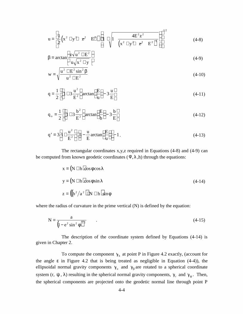
4-4
( ) ( )u x y z E
4E z
x y z E
2 2 2 22 2
2 2 2 2 2= + + − ⋅ + ++ + −
1
21 1
1 2
(4-8)
+
+=βyxu
Euzarctan
2
22
(4-9)
22
222
Eu
sinEuw
+β+= (4-10)
qu
E
E
u
u
E
2
2= +
−
1
21 3 3arctan (4-11)
qb
E
E
b
b
Eo
2
2= +
−
1
21 3 3arctan (4-12)
′ = +
⋅ −
−qu
E
u
E
E
u
2
23 1 1 1arctan . (4-13)
The rectangular coordinates x,y,z required in Equations (4-8) and (4-9) canbe computed from known geodetic coordinates ( φ , λ ,h) through the equations:
( ) λφ+= coscoshNx
( ) λφ+= sincoshNy (4-14)
( )( ) sinhNabz 22 φ+⋅=
where the radius of curvature in the prime vertical (N) is defined by the equation:
( ) 2122 sine1
aN
φ−= . (4-15)
The description of the coordinate system defined by Equations (4-14) isgiven in Chapter 2.
To compute the component hγ at point P in Figure 4.2 exactly, (account for
the angle ε in Figure 4.2 that is being treated as negligible in Equation (4-4)), theellipsoidal normal gravity components uγ and βγ are rotated to a spherical coordinate
system (r, ψ , λ) resulting in the spherical normal gravity components, rγ and ψγ . Then,
the spherical components are projected onto the geodetic normal line through point P

4-5
using the angular difference ( ψ−φ=α ) between geodetic (φ) and geocentric( ψ )
latitudes. The equations to calculate the exact value of hγ at point P follow:
( ) ( )αγ−αγ−=γ ψ sincosrh (4-16)
where from [33]
Eγr
Rγr
Sγr
RRES
R2SE1R12
System Spherical
rR =
Systemr Rectangulaz
y
xR
System lEllipsoida
u
γ=γ⇒
γγγ
→
γγγ
→
γγγ
⋅
λ
ψγ⋅γγ⋅=γ
λ
βrrrrrr
(4-17)
β+
β
λλβ−λβ+
λ−λβ−λβ+
=
0cosEuw
usin
w
1
cossinsinw
1sincos
Euw
u
sincossinw
1coscos
Euw
u
R
22
22
22
1 (4-18)
λλ−ψλψ−λψ−ψλψλψ
=0cossin
cossinsincossin
sinsincoscoscos
R 2 (4-19)
ψ−φ=α . (4-20)
The λγ component in the two normal gravity vectors, Eγr
and Sγr
, inEquation (4-17) is zero since the normal gravity potential is not a function of longitudeλ . The definitions for the other two relevant angles depicted in the Inset of Figure 4.2are:
α−θ=ε (4-21)
γγ
=θ ψ
r
arctan (4-22)
such that -π/2 ≤ θ ≤ π/2.

4-6
The equations listed here for the angles ( θεα ,, ) are applicable to both the northern andsouthern hemispheres. For positive h each of these angles is zero when point P is directlyabove one of the poles or lies in the equatorial plane. Elsewhere for h > 0 they have thesame sign as the geodetic latitude for point P. For h = 0 the angles, α and θ , are equaland ε = 0. Numerical results have indicated that the angular separation (ε) between the
component hγ and the total normal gravity vector totalγr
satisfies the inequality, ε < 4arcseconds, for geodetic heights up to 20,000 meters. For completeness the component
( φγ ) of the total normal gravity vector totalγr
at point P in Figure 4.2 that is orthogonal to
hγ and lies in the meridian plane for point P is given by the expression:
( ) ( )αγ+αγ−=γ ψφ cossinr . (4-23)
The component φγ has a positive sense northward. For geodetic height h=0 the φγcomponent is zero. Numerical testing with whole degree latitudes showed that themagnitude of φγ remains less than 0.002% of the value of hγ for geodetic heights up to
20,000 meters. Equations (4-16) and (4-23) provide an alternative way to compute the
magnitude totalγr
of the total normal gravity vector through the equation
22hotalt φγ+γ=γr .
In summary then, for near-surface geodetic heights when sub-microgalprecision is not necessary, the Taylor series expansion (4-3) for hγ should suffice. But,
when the intended application for hγ requires high accuracy, Equation (4-4) will be aclose approximation to the exact Equation (4-16) for geodetic heights up to 20,000meters. Of course, hγ can be computed using the exact Equation (4-16) but this requiresthat the computational procedure include the two transformations, R1 and R2, that areshown in Equation (4-17). Because the difference in results between Equations (4-4) and
(4-16) is less than one µgal(10-6 gal) for geodetic heights to 20,000 meters, thetransformation approach would probably be unnecessary in most situations. Forapplications requiring pure attraction (attraction without centrifugal force) due to thenormal gravitational potential V, the u- and β- vector components of normal gravitationcan be computed easily in the ellipsoidal coordinate system by omitting the last term inequations (4-5) and (4-6) respectively. These last attraction terms account for thecentrifugal force due to the angular velocity ω of the reference ellipsoid.

4-7
P(x,y,z).
βF1 F2. .
z
xy-plane
r
b
b’=u
Sphere of Radius r=a’
Confocal Ellipsoid Through Point P
Reference Ellipsoidal Surface So
b’=u=semi-minor axis a’=(u2+E2)1/2=semi-major axis
b=semi-minor axis a=semi-major axis
a
a’Ε
Ε=Focal Length =(a2-b2)1/2
Figure 4.1 Ellipsoidal Coordinates(u,β)
So
φ
Geodetic Normal
h
PO

4-8
Y(90o East)
φλ
P(φ,λ,h)
γh
X(0o East)
Equatorial Plane
yp
xp
zp
Geo
detic
Nor
mal
h
Rot
atio
n A
xis
Pole
Origin
Meridian Plane
Reference Ellipsoidal Surface
Z
Figure 4.2 Normal Gravity Component γh
Po
γh
α
γtotal
γψγr
P
ε
Inset
θ
ψ
Geo
cent
ric R
adiu
s
γφ

5-1
5. WGS 84 EGM96 Gravitational Modeling
5.1 Earth Gravitational Model (EGM96)
The form of the WGS 84 EGM96 Earth Gravitational Model is a sphericalharmonic expansion (Table 5.1) of the gravitational potential (V). The WGS 84EGM96, complete through degree (n) and order (m) 360, is comprised of 130,321coefficients.
EGM96 was a joint effort that required NIMA gravity data, NASA/GSFCsatellite tracking data, and DoD tracking data in its development. The NIMA effortconsisted of developing worldwide 30’ and 1° mean gravity anomaly databases from itsPoint Gravity Anomaly file and 5’ x 5’ mean GEOSAT Geodetic Mission geoid heightfile using least-squares collocation with the Forsberg Covariance Model [32] to estimatethe final 30’ x 30’ mean gravity anomaly directly with an associated accuracy. TheGSFC effort consisted of satellite orbit modeling by tracking over 30 satellites includingnew satellites tracked by Satellite Laser Ranging (SLR) , Tracking and Data RelaySatellite System (TDRSS), and GPS techniques, in the development of EGM96S (thesatellite only model of EGM96 to degree and order 70). The development of thecombination model to 70 x 70 incorporated direct satellite altimetry(TOPEX/POSEIDON, ERS-1, and GEOSAT) with EGM96S and surface gravity normalequations. Major additions to the satellite tracking data used by GSFC included newobservations of Lageos, Lageos-2, Ajisai, Starlette, Stella, TOPEX, GPSMET alongwith GEOS-1 and GEOSAT. Finally, GSFC developed the high degree EGM96solution by blending the combination solution to degree and order 70 with a blockdiagonal solution from degree and order 71 to 359 and a quadrature solution at degreeand order 360. A complete description of EGM96 can be found in [41].
The EGM96 through degree and order 70 is recommended for highaccuracy satellite orbit determination and prediction purposes. An Earth orbitingsatellite’s sensitivity to the geopotential is strongly influenced by the satellite’s altituderange and other orbital parameters. DoD programs performing satellite orbitdetermination are advised to determine the maximum degree and order that is mostappropriate for their particular mission and orbit accuracy requirements.
The WGS 84 EGM96 coefficients through degree and order 18 areprovided in Table 5.1 in normalized form. An error covariance matrix is available forthose coefficients through degree and order 70 determined from the weighted leastsquares combination solution. Coefficient sigmas are available to degree and order 360.Gravity anomaly degree variances are given in Table 5.2 for the WGS 84 EGM96(degree and order 360). Requesters having a need for the full WGS 84 EGM96, its errordata and associated software should forward their correspondence to the address listedin the PREFACE.

5-2
5.2 Gravity Potential (W)
The Earth’s total gravity potential (W) is defined as
W = V + Φ (5-1)
where Φ is the potential due to the Earth’s rotation. If ω is the angular velocity[Equation (3-6)], then
Φ = 12 ω( x2 + y2 ) (5-2)
where x and y are the geocentric coordinates of a given point in the WGS 84 referenceframe (See Figure 2.1).
The gravitational potential function (V) is defined as:
( )( )VGM
r
a
rP C m S m
n
nmm
n
n
n
nm nm= +
′ +
==∑∑1
02
sin cos sinmax
φ λ λ (5-3)
where:
V = Gravitational potential function (m2 /s2 )
GM = Earth’s gravitational constant
r = Distance from the Earth’s center of mass
a = Semi-major axis of the WGS 84 ellipsoid
n,m = Degree and order, respectively
φ′ = Geocentric latitude
λ= Geocentric longitude = geodetic longitude
C nm , S nm = Normalized gravitational coefficients

5-3
( )Pnm sin ′φ = Normalized associated Legendre function
( ) ( )( ) ( )=
− ++
′
n m n k
n mPnm
!
!sin
/2 1
1 2
φ
( )Pnm sin ′φ = Associated Legendre function
( )Pnm sin ′φ = ( )( )
( )[ ]cosd
d sinP
m
m n′′
′φφ
φmsin
( )Pn sin ′φ = Legendre polynomial
=( ) ( )1
2 n!
d
d sinsin 1
n
n
n2 n
′′ −
φφ
Note:
( )( ) ( )
C
S
n m
n m n k
C
Snm
nm
nm
nm
=+
− +
!
!
/
2 1
1 2
where:
C , Snm nm = Conventional gravitational coefficientsFor m=0, k=1;
m>1, k=2
The series is theoretically valid for r ≥ a, though it can be used with probably negligibleerror near or on the Earth’s surface, i.e., r ≥ Earth’s surface. But the series should not beused for r < Earth’s surface.

Table 5.1EGM96
Earth Gravitational ModelTruncated at n=m=18
E-03=X10 -3;E-05=X10-5;etc.
5-4
Degree and Order Normalized Gravitational Coefficientsn m Cnm Snm
2 0 -.484165371736E-03 2 1 -.186987635955E-09 .119528012031E-08 2 2 .243914352398E-05 -.140016683654E-05 3 0 .957254173792E-06 3 1 .202998882184E-05 .248513158716E-06 3 2 .904627768605E-06 -.619025944205E-06 3 3 .721072657057E-06 .141435626958E-05 4 0 .539873863789E-06 4 1 -.536321616971E-06 -.473440265853E-06 4 2 .350694105785E-06 .662671572540E-06 4 3 .990771803829E-06 -.200928369177E-06 4 4 -.188560802735E-06 .308853169333E-06 5 0 .685323475630E-07 5 1 -.621012128528E-07 -.944226127525E-07 5 2 .652438297612E-06 -.323349612668E-06 5 3 -.451955406071E-06 -.214847190624E-06 5 4 -.295301647654E-06 .496658876769E-07 5 5 .174971983203E-06 -.669384278219E-06 6 0 -.149957994714E-06 6 1 -.760879384947E-07 .262890545501E-07 6 2 .481732442832E-07 -.373728201347E-06 6 3 .571730990516E-07 .902694517163E-08 6 4 -.862142660109E-07 -.471408154267E-06 6 5 -.267133325490E-06 -.536488432483E-06 6 6 .967616121092E-08 -.237192006935E-06 7 0 .909789371450E-07 7 1 .279872910488E-06 .954336911867E-07 7 2 .329743816488E-06 .930667596042E-07 7 3 .250398657706E-06 -.217198608738E-06 7 4 -.275114355257E-06 -.123800392323E-06 7 5 .193765507243E-08 .177377719872E-07 7 6 -.358856860645E-06 .151789817739E-06 7 7 .109185148045E-08 .244415707993E-07 8 0 .496711667324E-07

Table 5.1EGM96
Earth Gravitational ModelTruncated at n=m=18
E-03=X10 -3;E-05=X10-5;etc.
5-5
Degree and Order Normalized Gravitational Coefficientsn m Cnm Snm
8 1 .233422047893E-07 .590060493411E-07 8 2 .802978722615E-07 .654175425859E-07 8 3 -.191877757009E-07 -.863454445021E-07 8 4 -.244600105471E-06 .700233016934E-07 8 5 -.255352403037E-07 .891462164788E-07 8 6 -.657361610961E-07 .309238461807E-06 8 7 .672811580072E-07 .747440473633E-07 8 8 -.124092493016E-06 .120533165603E-06 9 0 .276714300853E-07 9 1 .143387502749E-06 .216834947618E-07 9 2 .222288318564E-07 -.322196647116E-07 9 3 -.160811502143E-06 -.742287409462E-07 9 4 -.900179225336E-08 .194666779475E-07 9 5 -.166165092924E-07 -.541113191483E-07 9 6 .626941938248E-07 .222903525945E-06 9 7 -.118366323475E-06 -.965152667886E-07 9 8 .188436022794E-06 -.308566220421E-08 9 9 -.477475386132E-07 .966412847714E-07 10 0 .526222488569E-07 10 1 .835115775652E-07 -.131314331796E-06 10 2 -.942413882081E-07 -.515791657390E-07 10 3 -.689895048176E-08 -.153768828694E-06 10 4 -.840764549716E-07 -.792806255331E-07 10 5 -.493395938185E-07 -.505370221897E-07 10 6 -.375885236598E-07 -.795667053872E-07 10 7 .811460540925E-08 -.336629641314E-08 10 8 .404927981694E-07 -.918705975922E-07 10 9 .125491334939E-06 -.376516222392E-07 10 10 .100538634409E-06 -.240148449520E-07 11 0 -.509613707522E-07 11 1 .151687209933E-07 -.268604146166E-07 11 2 .186309749878E-07 -.990693862047E-07 11 3 -.309871239854E-07 -.148131804260E-06 11 4 -.389580205051E-07 -.636666511980E-07 11 5 .377848029452E-07 .494736238169E-07

Table 5.1EGM96
Earth Gravitational ModelTruncated at n=m=18
E-03=X10 -3;E-05=X10-5;etc.
5-6
Degree and Order Normalized Gravitational Coefficientsn m Cnm Snm
11 6 -.118676592395E-08 .344769584593E-07 11 7 .411565188074E-08 -.898252808977E-07 11 8 -.598410841300E-08 .243989612237E-07 11 9 -.314231072723E-07 .417731829829E-07 11 10 -.521882681927E-07 -.183364561788E-07 11 11 .460344448746E-07 -.696662308185E-07 12 0 .377252636558E-07 12 1 -.540654977836E-07 -.435675748979E-07 12 2 .142979642253E-07 .320975937619E-07 12 3 .393995876403E-07 .244264863505E-07 12 4 -.686908127934E-07 .415081109011E-08 12 5 .309411128730E-07 .782536279033E-08 12 6 .341523275208E-08 .391765484449E-07 12 7 -.186909958587E-07 .356131849382E-07 12 8 -.253769398865E-07 .169361024629E-07 12 9 .422880630662E-07 .252692598301E-07 12 10 -.617619654902E-08 .308375794212E-07 12 11 .112502994122E-07 -.637946501558E-08 12 12 -.249532607390E-08 -.111780601900E-07 13 0 .422982206413E-07 13 1 -.513569699124E-07 .390510386685E-07 13 2 .559217667099E-07 -.627337565381E-07 13 3 -.219360927945E-07 .974829362237E-07 13 4 -.313762599666E-08 -.119627874492E-07 13 5 .590049394905E-07 .664975958036E-07 13 6 -.359038073075E-07 -.657280613686E-08 13 7 .253002147087E-08 -.621470822331E-08 13 8 -.983150822695E-08 -.104740222825E-07 13 9 .247325771791E-07 .452870369936E-07 13 10 .410324653930E-07 -.368121029480E-07 13 11 -.443869677399E-07 -.476507804288E-08 13 12 -.312622200222E-07 .878405809267E-07 13 13 -.612759553199E-07 .685261488594E-07 14 0 -.242786502921E-07 14 1 -.186968616381E-07 .294747542249E-07

Table 5.1EGM96
Earth Gravitational ModelTruncated at n=m=18
E-03=X10 -3;E-05=X10-5;etc.
5-7
Degree and Order Normalized Gravitational Coefficientsn m Cnm Snm
14 2 -.367789379502E-07 -.516779392055E-08 14 3 .358875097333E-07 .204618827833E-07 14 4 .183865617792E-08 -.226780613566E-07 14 5 .287344273542E-07 -.163882249728E-07 14 6 -.194810485574E-07 .247831272781E-08 14 7 .375003839415E-07 -.417291319429E-08 14 8 -.350946485865E-07 -.153515265203E-07 14 9 .320284939341E-07 .288804922064E-07 14 10 .390329180008E-07 -.144308452469E-08 14 11 .153970516502E-07 -.390548173245E-07 14 12 .840829163869E-08 -.311327189117E-07 14 13 .322147043964E-07 .451897224960E-07 14 14 -.518980794309E-07 -.481506636748E-08 15 0 .147910068708E-08 15 1 .100817268177E-07 .109773066324E-07 15 2 -.213942673775E-07 -.308914875777E-07 15 3 .521392929041E-07 .172892926103E-07 15 4 -.408150084078E-07 .650174707794E-08 15 5 .124935723108E-07 .808375563996E-08 15 6 .331211643896E-07 -.368246004304E-07 15 7 .596210699259E-07 .531841171879E-08 15 8 -.322428691498E-07 .221523579587E-07 15 9 .128788268085E-07 .375629820829E-07 15 10 .104688722521E-07 .147222147015E-07 15 11 -.111675061934E-08 .180996198432E-07 15 12 -.323962134415E-07 .155243104746E-07 15 13 -.283933019117E-07 -.422066791103E-08 15 14 .519168859330E-08 -.243752739666E-07 15 15 -.190930538322E-07 -.471139421558E-08 16 0 -.315322986722E-08 16 1 .258360856231E-07 .325447560859E-07 16 2 -.233671404512E-07 .288799363439E-07 16 3 -.336019429391E-07 -.220418988010E-07 16 4 .402316284314E-07 .483837716909E-07 16 5 -.129501939245E-07 -.319458578129E-08

Table 5.1EGM96
Earth Gravitational ModelTruncated at n=m=18
E-03=X10 -3;E-05=X10-5;etc.
5-8
Degree and Order Normalized Gravitational Coefficientsn m Cnm Snm
16 6 .140239252323E-07 -.350760208303E-07 16 7 -.708412635136E-08 -.881581561131E-08 16 8 -.209018868094E-07 .500527390530E-08 16 9 -.218588720643E-07 -.395012419994E-07 16 10 -.117529900814E-07 .114211582961E-07 16 11 .187574042592E-07 -.303161919925E-08 16 12 .195400194038E-07 .666983574071E-08 16 13 .138196369576E-07 .102778499508E-08 16 14 -.193182168856E-07 -.386174893776E-07 16 15 -.145149060142E-07 -.327443078739E-07 16 16 -.379671710746E-07 .302155372655E-08 17 0 .197605066395E-07 17 1 -.254177575118E-07 -.306630529689E-07 17 2 -.195988656721E-07 .649265893410E-08 17 3 .564123066224E-08 .678327095529E-08 17 4 .707457075637E-08 .249437600834E-07 17 5 -.154987006052E-07 .660021551851E-08 17 6 -.118194012847E-07 -.289770975177E-07 17 7 .242149702381E-07 -.422222973697E-08 17 8 .388442097559E-07 .358904095943E-08 17 9 .381356493231E-08 -.281466943714E-07 17 10 -.388216085542E-08 .181328176508E-07 17 11 -.157356600363E-07 .106560649404E-07 17 12 .288013010655E-07 .203450136084E-07 17 13 .165503425731E-07 .204667531435E-07 17 14 -.141983872649E-07 .114948025244E-07 17 15 .542100361657E-08 .532610369811E-08 17 16 -.301992205043E-07 .365331918531E-08 17 17 -.343086856041E-07 -.198523455381E-07 18 0 .508691038332E-08 18 1 .721098449649E-08 -.388714473013E-07 18 2 .140631771205E-07 .100093396253E-07 18 3 -.507232520873E-08 -.490865931335E-08 18 4 .548759308217E-07 -.135267117720E-08 18 5 .548710485555E-08 .264338629459E-07

Table 5.1EGM96
Earth Gravitational ModelTruncated at n=m=18
E-03=X10 -3;E-05=X10-5;etc.
5-9
Degree and Order Normalized Gravitational Coefficientsn m Cnm Snm
18 6 .146570755271E-07 -.136438019951E-07 18 7 .675812328417E-08 .688577494235E-08 18 8 .307619845144E-07 .417827734107E-08 18 9 -.188470601880E-07 .368302736953E-07 18 10 .527535358934E-08 -.466091535881E-08 18 11 -.729628518960E-08 .195215208020E-08 18 12 -.297449412422E-07 -.164497878395E-07 18 13 -.627919717152E-08 -.348383939938E-07 18 14 -.815605336410E-08 -.128636585027E-07 18 15 -.405003412879E-07 -.202684998021E-07 18 16 .104141042028E-07 .661468817624E-08 18 17 .358771586841E-08 .448065587564E-08 18 18 .312351953717E-08 -.109906032543E-07

Table 5.2EGM96 Gravity Anomaly Degree Variances
Units = (1 x 10⁻⁵ m/second2 )2 or mgal2
5-10
Degree DegreeVariance
Degree DegreeVariance
Degree DegreeVariance
Degree DegreeVariance
2 7.6 39 3.3 76 2.7 113 2.7 3 33.9 40 2.8 77 2.9 114 3.0 4 19.8 41 3.1 78 2.9 115 3.1 5 21.0 42 3.4 79 3.0 116 2.6 6 19.7 43 3.0 80 2.8 117 2.7 7 19.6 44 3.0 81 3.5 118 2.8 8 11.2 45 3.4 82 4.0 119 2.8 9 11.2 46 3.8 83 3.7 120 2.7 10 9.8 47 3.7 84 3.0 121 2.5 11 6.6 48 3.2 85 2.9 122 2.2 12 2.7 49 2.7 86 3.4 123 2.7 13 7.9 50 3.6 87 3.0 124 2.4 14 3.5 51 3.0 88 2.9 125 2.8 15 3.7 52 3.1 89 2.8 126 2.8 16 4.1 53 4.0 90 2.4 127 3.0 17 3.2 54 3.6 91 3.1 128 2.2 18 3.9 55 3.2 92 3.0 129 2.4 19 3.2 56 3.8 93 3.0 130 2.2 20 3.1 57 3.8 94 3.1 131 2.3 21 3.7 58 3.0 95 3.0 132 2.2 22 3.5 59 3.6 96 2.4 133 2.5 23 3.1 60 3.2 97 2.9 134 2.3 24 2.4 61 3.1 98 3.2 135 2.3 25 3.1 62 3.3 99 2.7 136 2.4 26 2.4 63 3.2 100 2.8 137 2.3 27 1.7 64 2.8 101 2.1 138 2.6 28 3.0 65 2.7 102 2.9 139 2.1 29 2.6 66 3.2 103 3.5 140 2.4 30 2.9 67 3.2 104 2.8 141 2.2 31 2.7 68 3.2 105 2.4 142 1.8 32 2.7 69 3.4 106 2.8 143 2.1 33 3.0 70 2.5 107 2.7 144 2.3 34 4.0 71 2.6 108 2.9 145 2.0 35 3.9 72 3.4 109 2.8 146 2.0 36 3.3 73 2.8 110 3.3 147 2.1 37 3.5 74 3.7 111 2.9 148 2.0 38 3.0 75 2.9 112 2.5 149 2.0

Table 5.2EGM96 Gravity Anomaly Degree Variances
Units = (1 x 10⁻⁵ m/second2 )2 or mgal2
5-11
Degree DegreeVariance
Degree DegreeVariance
Degree DegreeVariance
Degree DegreeVariance
150 1.9 187 1.5 224 1.1 261 .7151 2.3 188 1.5 225 1.0 262 .6152 1.9 189 1.3 226 1.1 263 .7153 2.0 190 1.3 227 .9 264 .6154 1.7 191 1.4 228 1.0 265 .6155 2.1 192 1.6 229 1.1 266 .7156 1.9 193 1.5 230 1.0 267 .7157 1.9 194 1.3 231 1.1 268 .6158 1.7 195 1.4 232 1.1 269 .6159 2.0 196 1.3 233 1.0 270 .6160 1.7 197 1.3 234 1.0 271 .7161 1.8 198 1.4 235 1.0 272 .6162 2.0 199 1.3 236 1.0 273 .5163 2.0 200 1.3 237 .9 274 .6164 1.9 201 1.3 238 .9 275 .6165 2.1 202 1.2 239 .9 276 .6166 1.9 203 1.2 240 .9 277 .5167 2.0 204 1.3 241 .9 278 .6168 2.1 205 1.1 242 .9 279 .6169 1.8 206 1.2 243 .8 280 .6170 1.9 207 1.2 244 .8 281 .6171 1.9 208 1.2 245 .9 282 .6172 1.6 209 1.2 246 .9 283 .6173 1.7 210 1.4 247 .8 284 .5174 2.0 211 1.2 248 .7 285 .5175 1.7 212 1.2 249 .8 286 .5176 1.5 213 1.1 250 .9 287 .5177 1.6 214 1.3 251 .8 288 .5178 1.5 215 1.1 252 .9 289 .5179 1.8 216 1.1 253 .8 290 .5180 1.7 217 1.1 254 .7 291 .5181 1.5 218 1.1 255 .8 292 .5182 1.6 219 1.3 256 .7 293 .5183 1.5 220 1.1 257 .7 294 .5184 1.6 221 1.1 258 .7 295 .5185 1.4 222 1.1 259 .7 296 .5186 1.5 223 1.0 260 .7 297 .5

Table 5.2EGM96 Gravity Anomaly Degree Variances
Units = (1 x 10⁻⁵ m/second2 )2 or mgal2
5-12
Degree DegreeVariance
Degree DegreeVariance
Degree DegreeVariance
Degree DegreeVariance
298 .4 314 .4 330 .3 346 .3299 .4 315 .4 331 .3 347 .3300 .5 316 .4 332 .3 348 .3301 .5 317 .4 333 .3 349 .3302 .4 318 .5 334 .3 350 .3303 .5 319 .4 335 .3 351 .3304 .4 320 .4 336 .3 352 .3305 .4 321 .4 337 .3 353 .3306 .4 322 .4 338 .3 354 .3307 .4 323 .4 339 .3 355 .3308 .4 324 .4 340 .3 356 .3309 .5 325 .4 341 .4 357 .3310 .4 326 .4 342 .3 358 .3311 .4 327 .3 343 .3 359 .3312 .4 328 .4 344 .3 360 .3313 .4 329 .3 345 .3
The formula for computing gravity anomaly degree variances ( cn) is:
( ) ( )c n C Sn nm nmm
n
= − +=
∑γ 2 2 2 2
0
1
γ = Mean value of theoretical gravity (979764.32222 mgal).
C Snm nm, = normalized gravitational coefficients of degree (n) and order (m).

Units = (1 x 10⁻⁵ m/second2 )2 or mgal2
5-13

5- 14
This page is intentionally left blank

6-1
6. WGS 84 EGM96 GEOID
6.1 General
In geodetic applications three primary reference surfaces for the Earth areused: 1) the Earth’s topographic surface, 2) the geometric surface taken to be an ellipsoidof revolution, and 3) the geoid.
When the gravity potential (W) is a constant, equation (6-1), defines afamily of equipotential surfaces (geops) [33] of the Earth’s gravity field. The geoid is thatparticular geop that is closely associated with the mean ocean surface.
W(X,Y,Z) = constant (6-1)
Traditionally, when a geoid is developed, the constant (W), representing thepotential anywhere on this surface, is constrained or assumed to be equal to the normalpotential (U0) of a ‘best-fitting’ ellipsoid. Throughout this refinement effort, however,the authors recognize that the WGS 84 ellipsoid no longer represents a true ‘best-fitting’ellipsoid. The difference between the WGS 84 semi-major axis and the current ‘best-fitting’ value is 0.54 m. In terms of the geoid, this effect is handled through applicationof a ‘zero-order’ undulation (N0) of the geoid. With this approach, the WGS 84 ellipsoidcan be retained with no introduction of any additional errors by not using the “best-fitting” ellipsoid.
In common practice the geoid is expressed at a given point in terms of thedistance above (+N) or below (-N) the ellipsoid. For practical reasons, the geoid has beenused to serve as a vertical reference surface for mean sea level (MSL) heights. In areaswhere elevation data are not available from conventional leveling, an approximation ofmean sea level heights, using orthometric heights, can be obtained from the followingequation [33]:
h = H + N (6-2)H = h - N (6-3)
where:
h = geodetic height (height relative to the ellipsoid)N = geoid undulationH = orthometric height (height relative to the geoid)
Alternatively, some countries replace orthometric heights with normalheights and geoid undulations with height anomalies. This use of height anomalieseliminates assumptions about the density of masses between the geoid and the ground.Therefore, equation (6-2) can be re-formulated as:

6-2
h = H + N = H* + ζ (6-4)
where:
H* = normal height
ζ = height anomaly
The telluroid is a surface defined where the normal potential U at everypoint Q is equal to the actual potential W at its corresponding point P on the Earth’ssurface [33]. The height anomaly is the distance between point Q on the telluroid andpoint P on the Earth’s surface.
Equation (6-3) illustrates the use of geoid undulations in the determinationof orthometric heights (H) from geodetic heights (h) derived using satellite positions(e.g., Global Positioning System) located on the Earth's physical surface or aboard avehicle operating near the Earth's surface.
6.2 Formulas, Representations and Analysis
A significant departure from past practices has been implemented in thedetermination of geoid undulations. The WGS 84 EGM96 Geoid Undulations are basedon height anomalies calculated from the WGS 84 EGM96 spherical harmonic coefficientscomplete to degree and order 360. To transform from height anomalies to geoidundulations, the zero degree undulation term of -0.53 meters, and the WGS 84 EGM96correction coefficients through degree and order 360 are applied [34]. The value of -0.53meters is based on the difference between an “ideal” Earth ellipsoid in a tide free systemand the WGS 84 ellipsoid. The “ideal” ellipsoid was defined from the report of theInternational Association of Geodesy (IAG) Special Commission on FundamentalConstants [23]. The “ideal” Earth ellipsoid, in a ‘tide-free’ system, is defined by a =6378136.46 meters and 1/f = 298.25765.
6.2.1 Formulas
The formula for calculating the WGS 84 EGM96 Geoid Undulationsstarts with the calculation of the height anomaly ζ [34]:
( ) ( ) ( ) ( ) ( )ζ φ λγ φ
λ λ φ, , cos sin sinrGM
r
a
r
nCnm m Snm m Pnm
m
n
n
m= +
=∑
=∑
02
(6-5)

6-3
where: Cnm and Snm are the fully normalized potential coefficients of degree n and order
m from EGM96. Equation (6-5) is evaluated at a point P(φ,λ,r) on or above the surface ofthe earth:
GM = The Earth’s gravitational constant
r = Geocentric distance to the point P
a = Semi-major axis of the reference ellipsoid.
φ = Geocentric latitude
All quantities in formula (6-5) are defined for the WGS 84 EGM96with one exception. In equation (6-5), the even zonal coefficients of subscripts 2 through10 are coefficient differences between the dynamic WGS84 EGM96 and geometricallyimplied coefficients.
Cn Cn dynamic Cn geometric, ( ) , ( )0 0 0= −,
Table 6.1Geometric Coefficients
C geometric2 0, ( )-0.484166774985E-03
C geometric4 0, ( )0.790303733511E-06
C geometric6 0, ( )-0.168724961151E-08
C geometric8 0, ( )0.346052468394E-11
C geometric10 0, ( )-0.265002225747E-14
To calculate the geoid undulation N(in meters) we use the formula[41]:
( )N φ λ, = N 0 + ( )ζ φ λ, , r +( ) ( )∆g
HBA φ λγ
φ λ,
, (6-6)
where:N 0 = -0.53 meters (zero degree term)
and the parameters to compute the correction term discussed in section 6.2 above are:

6-4
( )∆g BA φ λ, = Bouguer gravity anomaly from EGM96
γ = Average value of normal gravity
( )H φ λ, = defined from harmonic analysis of JGP95E (Joint Gravity Project 95)
elevation database
The Bouguer anomaly can be computed from the EGM96 sphericalharmonic set and the harmonic analysis of the JGP95E elevation database. JGP95E is theworldwide 5’ digital elevation file developed by NIMA and NASA/GSFC from bestavailable sources for the EGM96 project.
( ) ( ) ( )∆ ∆g g HBA FAφ λ φ λ φ λ, , . ,= − ×0 1119 (6-7)
where:( )∆g FA φ λ, = Free-air gravity anomaly from EGM96
6.2.2 Permanent Tide Systems
In the calculation of geoid undulations from the EGM96Geopotential Model the second degree zonal coefficient is given in the tide-free system.The tide-free definition means that any geoid undulations calculated from EGM96 existfor a tide-free Earth with all (direct and indirect) effects of the sun and moon removed.Other geoids to consider are the mean geoid (geoid which would exist in the presence ofthe sun and moon) and the zero geoid (geoid which exists if the permanent direct effectsof the sun and moon are removed but the indirect effect related to the Earth’s elasticdeformation is retained). A complete set of equations to convert from one tide system toanother can be found in [35].
To calculate the geoid in the zero tide system use the formula:
N NZ n= + −2 97 888 2. . sin φ cm (6-8)where:
N Z = zero-tide geoid
N n = tide-free geoid
6.2.3 Representations and Analysis
The geoid undulations can be depicted as a contour chart whichshows the deviations of the geoid from the ellipsoid selected as the mathematical figureof the Earth. Figure 6.1 is a worldwide WGS 84 EGM96 Geoid Undulation ContourChart developed from a worldwide 15’x15’ grid of geoid undulations calculated by usingWGS 84 parameters and the WGS 84 EGM96 coefficients through n=m=360 in Equation(6-6).

6-5

6-6
The WGS 84 EGM96 Geoid Undulations, taken worldwide on the basis of a 15’x15’grid, exhibit the following statistics:
Mean = -0.57 metersStandard Deviation = 30.56 metersMinimum = -106.99 metersMaximum = 85.39 meters
Location of Minimum: φ = 4.75° N , λ = 78.75° EMaximum: φ = 8.25° S , λ = 147.25° E
This standard deviation indicates the typical difference between the geoid and thereference ellipsoid.
The WGS 84 EGM96 Geoid Undulations have an error range of+0.5 to +1.0 meters (one sigma) worldwide.
6.3 Availability of WGS 84 EGM96 Data Products
The WGS 84 EGM96 standard products are:
• A 15’ x 15’ WGS 84 EGM96 Geoid Undulation file calculated from equation(6-6).
• The EGM96 spherical harmonic coefficients complete to degree and order 360.
Additional information on the WGS 84 EGM96 Geoid Undulations,associated software and data files can be obtained from the location and addresses in thePREFACE.

7-1
7. WGS 84 RELATIONSHIPS WITH OTHER GEODETIC SYSTEMS
7.1 General
One of the principal purposes of a world geodetic system is to eliminatethe use of local horizontal geodetic datums. Although the number of local horizontalgeodetic datums, counting island and astronomic-based datums, exceeds severalhundred, the number of local horizontal datums in current use is significantly less andcontinues to decrease. Until a global geodetic datum is accepted, used and implementedworldwide, a means to convert between geodetic datums is required. To accomplish theconversion, local geodetic datum and WGS coordinates are both required at one or moresites within the local datum area so that a local geodetic datum to WGS datum shift canbe computed. Satellite stations positioned within WGS 84, with known local geodeticdatum coordinates, were the basic ingredients in the development of local geodeticdatum to WGS 84 datum shifts.
Local horizontal datums were developed in the past to satisfy mapping andnavigation requirements for specific regions of the Earth. A geocentric datum of largegeographic extent is the North American Datum 1983 (NAD 83). In the past couple ofdecades, development of global geocentric datums has become possible. WGS 84 andthe ITRF are examples of such datums.
The most accurate approach for obtaining WGS 84 coordinates is toacquire satellite tracking data at the site of interest and position it directly in WGS 84using GPS positioning techniques. Direct occupation of the site is not always possibleor warranted. In these cases, a datum transformation can be used to convert coordinatesfrom the local system to WGS 84.
7.2 Relationship of WGS 84 to the ITRF
As discussed in Chapter 2, the WGS 84 is consistent with ITRF. Thedifferences between WGS 84 and ITRF are in the centimeter range worldwide.Therefore, for all mapping and charting purposes, they can be considered the same.
In recent years, some countries and regions have been converting todatums based on the ITRF. Such national or regional datums that are rigorously basedon the ITRF can also be considered as identical to WGS 84. An example of such adatum is the European Terrestrial Reference Frame 1989 (EUREF89).
7.3 Relationship of WGS 84 to NAD 83
The North American Datum 1983 (NAD 83) is a geocentric datum thatwas established in 1986 for the United States, Canada, Mexico, Central America and theCaribbean Islands. Hawaii and Greenland were also connected to this datum. It is

7-2
based on a horizontal adjustment of conventional survey data and the inclusion ofTransit Satellite Doppler data and Very Long Baseline Interferometry (VLBI) data. Theglobal Doppler and VLBI observations were used to orient the NAD 83 reference frameto the BIH Terrestrial System of 1984. The orientation of the ECEF coordinate axes ofthe NAD 83 reference frame is identical to that of the original WGS 84 reference frame.
NAD 83 uses the Geodetic Reference System 1980 (GRS 80) ellipsoid asits reference ellipsoid with the geometric center of the ellipsoid coincident with thecenter of mass of the Earth and the origin of the coordinate system. The semi-majoraxis and flattening parameters are adopted directly as
a = 6378137 m1/f = 298.257222101
The WGS 84 ellipsoid is for all practical purposes identical to the GRS 80ellipsoid. They use the same value for the semi-major axis and have the sameorientation with respect to the center of mass and the coordinate system origin.However, WGS 84 uses a derived value for the flattening that is computed from thenormalized second-degree zonal harmonic gravitational coefficient C2 0, . C2 0, was
derived from the GRS 80 value for J2 and truncated to 8 significant digits as:
C2 0, = -J2/(5)1/2. (7-1)
The resulting WGS 84 value for 1/f is 298.257223563. The differencebetween the GRS 80 and WGS 84 values for f creates a difference of 0.1 mm in thederived semi-minor axes of the two ellipsoids.
Based on these definitions, geodetic positions determined with respect toNAD 83 or WGS 84 have uncertainties of about one meter in each component. Formapping, charting and navigation, the two systems are indistinguishable at scales of1:5,000 or smaller and with accuracies of about 2 m. Note that the National MapAccuracy Standard requires points to be horizontally accurate to 0.51 mm (1/50 in.) forscales of 1:20,000 or larger and 0.84 mm (1/30 in.) for scales less than 1:20,000. Forexample, this corresponds to 2.5 m at 1:5,000 and 42 m at 1:50,000. For geodeticapplications, one can expect to see a difference of a meter or more between the WGS 84and NAD 83 positions of the same point. This is due to the uncertainty associated witheach independent determination and the fact that the errors are additive when comparingthe difference in the coordinates.
WGS 84 has undergone several enhancements since its original definition.The practical realization of the reference frame is determined by a network of permanentGPS tracking stations which are aligned with the ITRF, the successor to the BIHTerrestrial System, through a globally distributed set of stations with very high accuracy

7-3
ITRF coordinates. The improved WGS 84 reference frame is coincident with the ITRFat the 5 cm level. WGS 84 geodetic positions can be determined with uncertainties atthe 25-50 cm level or better in a component depending upon the technique. Theseenhancements have had no effect on mapping, charting and navigation applicationssince they are at the meter level or smaller.
Meanwhile, the NOAA’s National Geodetic Survey has established HighAccuracy Reference Networks (HARNs) in many states in the U.S. using GPStechniques. HARNs in effect represent an upgrading of the original NAD 83 geodeticcontrol networks. The new networks have relative accuracies 1-2 orders of magnitudebetter than the original networks that define NAD 83. Each state’s HARN is adjustedseparately but is tied to a national network of the highest accuracy points. There can bedifferences of 0.3 to 0.8 m between the original NAD 83 coordinates and the new ones.Thus, although both NAD 83 and WGS 84 have undergone improvements in accuracyand precision, coordinates determined in one system will differ from coordinatesdetermined in the other system for a specific point. These differences may be on theorder of one meter or less and are due to systematic differences of the reference framescombined with random errors associated with the GPS observations.
7.4 Local Geodetic Datum to WGS 84 Datum Transformations
For most applications and DoD operations involving maps, charts,navigation and geospatial information, WGS 84 coordinates will be obtained from aLocal Geodetic Datum to WGS 84 Datum Transformation. This transformation can beperformed in curvilinear (geodetic) coordinates:
φWGS 84 = φLocal + ∆φ
λWGS 84 = λLocal + ∆λ (7-2)
hWGS 84 = hLocal + ∆h
where ∆φ, ∆λ, ∆h are provided by the Standard Molodensky transformation formulas[36], [37]:
∆φ” = {- ∆X sin φ cos λ - ∆Y sin φ sin λ + ∆Z cos φ + ∆a (RN e2 sin φ cos φ)/a + ∆f [RM
(a/b)+ RN (b/a)] sin φ cos φ} • [(RM+ h) sin 1" ]-1
∆λ” = [- ∆X sin λ + ∆Y cos λ] • [(RN + h) cos φ sin 1” ]-1
∆h = ∆X cos φ cos λ + ∆Y cos φ sin λ + ∆Z sin φ - ∆a (a/RN ) + ∆f (b/a) RN sin2 φ

7-4
where: φ, λ, h = geodetic coordinates (old ellipsoid)
φ = geodetic latitude. The angle between the plane of the geodetic equator and theellipsoidal normal at a point (measured positive north from the geodetic equator,negative south).
λ = geodetic longitude. The angle between the plane of the Zero Meridian and theplane of the geodetic meridian of the point (measured in the plane of the geodeticequator, positive from 0° to 180° E, and negative from 0° to 180° W).
h = N + H
where:
h = geodetic height (height relative to the ellipsoid)
N = geoid height
H = orthometric height (height relative to the geoid)
∆φ, ∆λ, ∆h = corrections to transform local geodetic datum coordinates to WGS84 φ, λ, h values. The units of ∆φ and ∆λ are arc seconds ("); the units of ∆h are meters(m).‘NOTE: AS "h's" ARE NOT AVAILABLE FOR LOCAL GEODETIC DATUMS, THE∆h CORRECTION WILL NOT BE APPLICABLE WHEN TRANSFORMING TOWGS 84.
∆X, ∆Y, ∆Z = shifts between centers of the local geodetic datum andWGS 84 ellipsoid; corrections to transform local geodetic system-related rectangularcoordinates (X, Y, Z) to WGS 84-related X, Y, Z values.
a = semi-major axis of the local geodetic datum ellipsoid.
b = semi-minor axis of the local geodetic datum ellipsoid.
b/a = 1 - f
f = flattening of the local geodetic datum ellipsoid.
∆a, ∆f = differences between the semi-major axis and flattening of thelocal geodetic datum ellipsoid and the WGS 84 ellipsoid, respectively (WGS 84 minusLocal).

7-5
e = first eccentricity.
e2 = 2f - f2
RN = radius of curvature in the prime vertical.
RN = a/(l- e2 sin2 φ)1/2
RM = radius of curvature in the meridian.
RM = a(l- e2 )/(l- e2 sin2 φ)3/2
NOTE: All ∆-quantities are formed by subtracting local geodetic datum ellipsoid valuesfrom WGS 84 Ellipsoid values.
Appendix A lists the reference ellipsoid names and parameters (semi-major axis and flattening) for local datums currently tied to WGS 84 and used forgenerating datum transformations.
Appendix B contains horizontal transformation parameters for the geodeticdatums/systems which have been generated from satellite ties to the local geodeticcontrol. Due to the errors and distortion that affect most local geodetic datums, use ofmean datum shifts (∆X, ∆Y, ∆Z) in the Standard Molodensky datum transformationformulas may produce results with poor quality of "fit". Improved fit between the localdatum and WGS 84 may result only with better and more dense ties with local orregional control points.
Updates to the datum transformation parameters are identified through theuse of cycle numbers and issue dates. Cycle numbers have been set to the numericalvalue of zero for all datum transformations appearing in the August 1993 Insert 1 andthe WGS 84 TR8350.2 Second Edition. All new datum transformations will carry acycle number of zero. As updates are made the cycle number will increment by one.
Datum transformation shifts derived from non-satellite information arelisted in Appendix C.
7.5 Datum Transformation Multiple Regression Equations (MRE)
The development of Local Geodetic Datum to WGS 84 DatumTransformation Multiple Regression Equations [38] was initiated to obtain better fitsover continental size land areas than could be achieved using the Standard Molodenskyformula with datum shifts (∆X, ∆Y, ∆Z).

7-6
For ∆φ, the general form of the Multiple Regression Equation is (also see[38]):
∆φ = A0 + A1 U + A2 V + A3 U2 + A4 UV + A5 V
2 +...+ A99 U9 V9 (7-3)
where:
A0 = constant
A0, A1,... An n = coefficients determined in the development
U = k ( φ − φm ) = normalized geodetic latitude of the computation point
V = k ( λ − λm ) = normalized geodetic longitude of the computation point
k = scale factor, and degree-to-radian conversion
φ, λ = local geodetic latitude and local geodetic longitude (in degrees),respectively, of the computation point
φm, λm = mid-latitude and mid-longitude values, respectively, of the local geodeticdatum area (in degrees).
Similar equations are obtained for ∆λ and ∆h by replacing ∆φ in the leftportion of Equation (7-3) by ∆λ and ∆h, respectively.
Local Geodetic Datum to WGS 84 Datum Transformation MultipleRegression Equations for seven major continental size datums, covering contiguouscontinental size land areas with large distortion, are provided in Appendix D. The mainadvantage of MREs lies in modeling of distortion for better fit in geodetic applications.However, caution must be used to ensure that MREs are not extrapolated outside of thearea of intended use. Large distortions can be realized in very short distances outside ofthe area where the stations that were used in the development of the MREs exist.
7.6 WGS 72 to WGS 84
See Appendix E.

8-1
8. ACCURACY OF WGS 84 COORDINATES
8.1 Discussion
Numerous techniques now exist to establish WGS 84 coordinates for agiven site. The accuracy and precision achieved by these various techniques varysignificantly. The most common, currently-available techniques are listed below:
• General geodetic solution for station coordinates, orbits, and otherparameters of interest.
• Direct geodetic point positioning at a stationary, solitary station using a’geodetic-quality’, dual frequency GPS receiver and NIMA PreciseEphemerides and Satellite Clock states (note that the effects ofSelective Availability (SA) must be removed).
• Same as above but using the Broadcast GPS Ephemerides and ClockStates.
• GPS differential (baseline) processing from known WGS 84 sites
• GPS Precise Positioning Service (PPS) navigation solutions• Instantaneous• Mean over some averaging interval
• GPS Standard Positioning Service (SPS) navigation solutions• Instantaneous• Mean over some averaging interval
• Photogrammetrically-derived coordinates from NIMA products
• Map-derived coordinates from digital or paper NIMA products Clearly, the above positioning techniques do not provide WGS 84
coordinates with uniform accuracy and statistical properties. Even within a giventechnique, accuracy variations can occur, due for example, to the treatment of certainerror sources such as the troposphere. Because of these variations and periodic algorithmimprovements, full characterization of the accuracy achieved by all the above techniqueswould be quite challenging and beyond the scope of this document.
In the terminology of Chapter 2, a network of stations obtained from one ofthese techniques yields a unique realization of the WGS 84 reference frame. Currently,within the DoD, almost all operational geodetic survey requirements can be met withdirect geodetic point positioning with GPS. The NIMA-developed technique [39] which

8-2
performs this function has been demonstrated to achieve an accuracy at a single stationof:
1994-present: 30 cm (1σ), in each of the 3 position components (φ,λ,h)
1989-1994: 100 cm (1σ), in each of the 3 position components (φ,λ,h)
Under special circumstances, such as the refinement of the permanent DoDGPS tracking network coordinates, a general geodetic solution is performed where thepositions of the entire permanent global DoD network are estimated simultaneously withmany other parameters. This type of special technique, which was used to develop theWGS 84 (G873) reference frame, has demonstrated an accuracy of:
5cm (1σ), in each of the 3 position components (φ,λ,h)
Other techniques which are based on older, previously-established surveycoordinates can also yield ’WGS 84’ coordinates with limited accuracy. These techniquesmay be suitable for certain mapping applications but must be treated very cautiously if ahigh level of accuracy is required. Some of these alternate techniques to obtain WGS 84coordinates are listed below:
TRANSIT Point Positioning directly in WGS 84 (1σ= 1-2 m)
TRANSIT Point Positions transformed from NSWC-9Z2
GPS differential (baseline) processing from a known (TRANSIT-determined) WGS 84 geodetic point position
By a WGS 72 to WGS 84 Coordinate Transformation
By a Local Geodetic Datum to WGS 84 Datum Transformation
Because geospatial information within the DoD often originates frommultiple sources and processes, the absolute accuracy of a given WGS 84 positionbecomes very important when information from these various sources is combined in’Geographic Information Systems’ or ’geospatial databases’. Because of their high fidelity,surveyed WGS 84 geodetic control points can often serve to improve or validate theaccuracy of maps, image products or other geospatial information. Even GPS navigationsolutions can serve a similar role, as long as the accuracy of these solutions is well-understood.

8-3
8.2 Summary
In summary, while WGS 84 provides a common global framework for allgeospatial information within the DoD, the accuracy of each ’layer’ of informationdepends largely on the metric fidelity of the process used to collect that information.WGS 84 surveyed control points provide an accuracy level which meets or exceeds allcurrent operational DoD requirements.

8-4
This page is intentionally left blank

9-1
9. IMPLEMENTATION GUIDELINES
9.1 Introduction
WGS 84 represents the current state-of-the-art DoD operational referencesystem which has been derived from the best available satellite tracking, satellitealtimeter and surface gravity data. It supports the most stringent accuracy requirementsfor geodetic positioning, navigation and mapping within DoD. It is the policy of NIMAto continually improve components of the WGS 84 system to maintain it as a state-of-the-art DoD operational World Geodetic System. This will lead to improvements in thedefinition and realization of the system as:
• The basic tracking stations which are used are updated, repositioned ortheir number is increased.
• Additional data makes it possible to improve the accuracy ofindividual local datum relationships to WGS 84.
• Additional surface gravity data become available in various areas ofthe world to improve the gravity and geoid models.
The current definition of WGS 84 recognizes the continually changingphysical Earth, shifting of internal masses and continental plate motions, andaccommodates this time dependency in its definition through a plate motion model. Forthe high accuracy geodetic positioning requirements, this requires a time epoch to bedefined for all station coordinates, since they are in continual motion. As mentionedpreviously in this report, the coordinates of the fixed GPS tracking stations (WGS84(G873)) were implemented into the production of the NIMA precise orbits starting atGPS week 873 (September 29, 1996), with an epoch of 1997.0.
As a consequence of the inherent high accuracy and continual refinement ofthe definition and realization of WGS 84, considerable care should be taken in theimplementation of this system into existing and future weapons systems and geospatialinformation systems. This Chapter will address some of the considerations that should bemade prior to the implementation of WGS 84 to ensure that the full benefits of WGS 84are realized and are consistent with the operational product accuracy and interoperabilityrequirements of the users. Careful consideration by the user of the products and accuracysupported by the implementation can lead to reduced costs and reduced effort in theimplementation of WGS 84 with no loss of accuracy of the product. The guidelinespresented in this Chapter are organized around basic classes of users: precise highaccuracy geodetic users, cartographic users, navigation users, and geospatial informationusers. The absolute accuracy requirements vary significantly between these applicationsranging from centimeter requirements for precise geodetic positioning to hundreds ofmeters for small scale maps. These recommendations are provided to stimulate users to

9-2
analyze their specific implementation to determine how best to implement WGS 84 dataand information, rather than a complete implementation which may not be necessary.
9.1.1 General Recommendations
Before satellite geodetic techniques became available, the localhorizontal datum was defined independently of the local vertical datum. NIMA hasdeveloped datum transformations to convert over 120 local horizontal datums to WGS84. This generally entails making survey ties between a number of local geodetic controlpoints and their corresponding geodetic positions derived from satellite observations.NIMA did this for many years with Doppler observations from TRANSIT satellites andcontinues to do it now with GPS. Aside from the countless maps and charts which arestill based on these classical local datums, numerous land records, property boundariesand other geographic information in many countries are referenced to local datums.There is currently no world vertical system defined to unify and tie together these localvertical systems. Generally the vertical datum is defined by a series of tide gauges in thearea or by approximating mean sea level by the geoid leading to numerous realizations ofmean sea level. Unfortunately, the local geodetic coordinates on these datums are oflimited use for modern survey, navigation and mapping operations. Modern maps,navigation systems and geodetic applications require a single accessible, global, 3-dimensional reference frame. It is important for global operations and interoperabilitythat DoD systems implement and operate as much as possible on WGS 84. It is equallyimportant that systems implement the WGS 84 information relative to the gravity field,geoid and datum transformations in a manner that will allow future update of specificportions of the data.
These data will change with future refinements of WGS 84, asimproved information becomes available to NIMA, and this may necessitate updates toexisting implementations as future operational accuracy requirements become known.For example, implementations of the geoid undulation values as a grid in a lookup tablewould facilitate easier future updates than implementation as spherical harmoniccoefficients.
9.1.2 Precise Geodetic Applications
For precise surveying applications, full implementation isrecommended. This will provide the user with the ultimate positioning accuracy in WGS84. It is further recommended that in these applications coordinates be maintained withan epoch assigned to each coordinate determination along with an indication of the fixedstation GPS coordinate set used for the realization, such as WGS 84(G873). The EGM96 through degree and order 70 is recommended for high accuracy satellite orbitdetermination and prediction purposes. An Earth orbiting satellite’s sensitivity to thegeopotential is strongly influenced by the satellite’s altitude range and other orbitalparameters. DoD programs performing satellite orbit determination are advised to

9-3
determine the maximum degree and order most appropriate for their particular missionand orbit accuracy requirements.
9.1.3 Cartographic Applications
The original definition and realization of WGS 84 still satisfies theDoD’s mapping and charting requirements. The 1-2 meter accuracy (lσ) of the WGS 84reference frame, as defined in TR8350.2, Second Edition, is more than adequate for largescale mapping. The current national horizontal map accuracy standard indicates that welldefined points should be located with an accuracy better than 1/30 of an inch (0.84 mm)at a 90 percent confidence level on maps with scales greater than 1:20,000. Thistranslates to 8.4 m on a 1:10,000 scale map which is easily met by WGS 84, TR8350.2,Second Edition, assuming, of course, that the mapping products are on WGS 84 and not alocal datum. If the maps or charts are on local datums, then the application of appropriatedatum transformations is necessary to preserve interoperability with other geospatialinformation. Depending on the local datum, the accuracy of the datum transformationscan vary from 1 meter to over 25 meters in each component.
The vertical accuracy of geospatial information and resulting mapproducts depends on how the elevations were compiled. If the elevations are based onfirst order geodetic leveling, the control heights are very accurate, probably good tocentimeters with respect to ’local mean sea level’. A height bias in the local mean sealevel would be the major potential error source. If no leveling data are available forvertical control, elevations are estimated from height above the WGS 84 referenceellipsoid and a geoid height derived from the WGS 84 geoid model. For mappingprocesses which use imagery, the orthometric heights (height above the geoid) aresubstituted for elevations above mean sea level. For these products the EarthGravitational Model 1996 (EGM96), which provides a geoid with an accuracy of 0.5 - 1.0m. worldwide, should be implemented, especially for scales 1:10,000 or larger.
Consequently, for mapping implementation, it is very important tohave the product accuracy in mind when implementing the refinements as defined in thisdocument. Specifically, all datum transformations listed in this report may not benecessary, especially the regional values. The full resolution of the geoid may also not benecessary based on the changes of this geoid from the geoid documented in WGS 84,TR8350.2, Second Edition. Implementation on a 30 minute or 1 degree grid may be morethan adequate. Neither does there appear to be a reason to implement the geoid asspherical harmonics.
9.1.4 Navigation Applications
The navigator represents a user with applications distinct from thosediscussed above. The navigator is moving and positioning in real-time or after the fact onland, air and sea platforms. Accuracy requirements may vary from the centimeter level

9-4
for precise geodetic applications, such as aerial photogrammetry, to meters for combinedintegrated GPS/Inertial Navigation Systems, to tens of meters for the SPS GPS user.Navigation applications are also characterized by large numbers of systems in the field,e.g. more than 100,000 GPS military receivers, with legacy systems having differentimplementations of WGS 84 than the newer systems. Implementation and update ofWGS 84 in these platforms are costly and almost impossible to accomplishsimultaneously. Therefore, a careful analysis must be done for each implementation todetermine the essential elements of the refined definition of WGS 84 that need to beimplemented. A few suggestions are offered:
The implementation of the geoid in these applications should be as alookup table with an appropriate interpolation scheme. To help in deciding the gridinterval, a comparison should be made of the errors introduced in the geoid heightsutilizing various grid sizes. All applications may not require the maximum resolution.
Cycle numbers have been provided to document the datumtransformation changes. This makes it possible for the user to tell if an update has beenmade to a specific transformation.
In some cases, the mean datum transformations may be sufficient forthe user’s requirements. Implementation of regional datum transformations may not berequired. Use of the regional transformations versus the mean datum transformationsshould be analyzed with respect to the system accuracy capabilities.
9.1.5 Geospatial Information Applications
Geospatial databases contain information from various sources asthematic layers from which imagery, imagery intelligence, and geospatial information canbe derived or extracted. Since the informaton represented in the various layers hasmultiple uses and supports applications of different accuracies, it is important that theaccuracy of the basic information be retained. Therefore, the refined WGS 84 should beimplemented in geospatial systems to maintain the inherent accuracy of the basic datasources.
9.2 Summary
Users need to implement the refinements of the WGS 84 (TR8350.2,Third Edition) into application systems in a planned and well thought out manner. Ananalysis into what aspects of these refinements are required for specific applicationsshould be performed. This will ensure that the applications have indeed implementedWGS 84 (TR8350.2, Third Edition), in the most effective manner.

10-1
10. CONCLUSIONS/SUMMARY
The refined World Geodetic System 1984 is based on the use of data, techniques,and technology available in early 1997. As a result, the refined WGS 84 is more accuratethan its predecessor and replaces it as the three dimensional geodetic system officiallyauthorized for DoD use.
Major changes in this report are as follows:
• Refined Earth Gravitational Model complete to degree and order 360.
• New geoid undulations accurate from ±0.5 meter to ±1.0 meter.
• Additional and improved datum transformation parameters from local to WGS84.
• Modifications to the ellipsoidal (normal) gravity model.
• New Earth Gravitational Constant (GM).
• New realization of the WGS 84 (G873) reference frame through a moreaccurate determination of NIMA and Air Force GPS monitor stations.
• Inclusion of a new chapter on implementation guidance.
The value of WGS 84 will become increasingly evident with the expansion ofgeospatial databases and information systems. Accurate coordinates will ensureconsistency, interoperability and accuracy between thematic data layers. Since thereference system for NAVSTAR GPS is WGS 84, high quality geodetic coordinates areprovided automatically by NAVSTAR GPS User Equipment. For those using NAVSTARGPS but still utilizing local geodetic datums and products, the availability of the moreaccurate WGS 84 to Local Geodetic Datum Transformations leads to an improvedrecovery of local coordinates.
NIMA will continually review DoD requirements and assure that WGS 84 willremain a dynamic viable system which meets or exceeds these requirements.

10-2
This page is intentionally left blank

R-1
REFERENCES
1. IERS Technical Note 21, IERS Conventions (1996), D. McCarthy, editor,Observatoire de Paris; l July 1996.
2. Mueller, I.; “Reference Coordinate Systems and Frames: Concepts andRealizations”; Bulletin Geodesique; Vol. 59; 1985.
3. Cunningham, J.P.; “Determination of TRANET and SMTP Tracking StationCoordinates for Use in the WGS 84”; NSWC TR 87-61; Naval Surface WarfareCenter, Dahlgren, Va.; June 1987.
4. Fell, P., Swift, E.R., Cunningham, J. and Malys, S.; “Bridging the Gap BetweenTRANSIT and GPS Point Positioning - The Implications of Higher OrderIonospheric Refraction on the Realization of the WGS 84 Reference Frame”;NSWCDD TR 92-557; October 1992.
5. Malys, S.; Dispersion and Correlation Among Transformation Parameters RelatingTwo Satellite Reference Frames; Ohio State Univ. Dept. of Geodetic Science andSurveying Report No. 392; July 1988.
6. Malys, S.; “Similarity Transformation Between NAVSAT and GPS ReferenceFrames”; American Geophysical Union Chapman Conference on GPSMeasurements for Geodynamics; Ft. Lauderdale, Fl.; September 1988.
7. Swift, E.R.; “Preliminary Comparison of the WGS 84 and SV5 Reference FramesUsing GPS Pseudorange Data”; Proceedings of the Sixth International GeodeticSymposium on Satellite Positioning; Columbus, Ohio; March 1992.
8. Swift, E.R.; “Improved WGS 84 Coordinates for the DMA and Air Force GPSTracking Sites”; Proceedings of ION GPS-94; Salt Lake City, Utah; September1994.
9. Cunningham, J. and Curtis, V. L.; “WGS 84 Coordinate Validation andImprovement for the NIMA and Air Force GPS Tracking Stations”;NSWCDD/TR-96/201; November 1996.
10. Malys, S. and Slater, J.A.; “Maintenance and Enhancement of the World GeodeticSystem 1984”; Proceedings of ION GPS-94; Salt Lake City, Utah; September 1994.

R-2
11. Cunningham, J.P. and Curtis, V.L.; “Estimating GPS Orbits, Clocks andCovariances in Support of SATRACK II”; NAVSWC TR 91-539; Dahlgren, Va.;August 1991.
12. DeMets, C.; Personal Communication; April 1997.
13. Moritz, H. and Mueller, I.I.; Earth Rotation-Theory and Observation; UngarPublishing Company; New York, New York; 1987.
14. Kaplan, G.H.; The IAU Resolutions on Astronomical Constants, Time Scales, andthe Fundamental Reference Frame; Circular No. 163; United States NavalObservatory; Washington, DC; 10 December 1981.
15. IERS Technical Note 13, IERS Conventions (1992), D. McCarthy, editor,Observatoire de Paris; July 1992.
16. ICD-GPS-211; Interface Control Document; “GPS Control Segment/ DMAInterfaces”; REV A; October 1991.
17. Bangert, J.A.; “The DMA / GPS Earth Orientation Prediction Service”; Proceedingsof the Fourth International Geodetic Symposium on Satellite Positioning; Austin,Texas; April, 1986.
18. Farrar, R., and Laing, P.A.; “Earth Orientation Prediction Accuracy”; AerospaceCorporation Report; TOR-96(1567)-1; 1996.
19. Kopcha. P.D., and van Gelder, B.H.W.; “A study of DMA's Prediction Accuracy onEarth Orientation Parameters”; Proceedings of ION-GPS-96; Kansas City,Missouri; September 1996.
20. Moritz, H.; "Geodetic Reference System 1980"; Bulletin Geodesique; Vol. 54, No.3; Paris, France; 1980.
21. DMA Letter; “Improved WGS 84 Coordinates and GM Value for Air Force andDefense Mapping Agency Global Positioning System Monitor Stations for HighAccuracy Satellite Orbit Determination”; Office Code OPG; 15 May 1994.
22. Moritz H.; "Fundamental Geodetic Constants"; Report of Special Study Group No.5.39 of the International Association of Geodesy (IAG); XVII General Assembly ofthe International Union of Geodesy and Geophysics (IUGG); Canberra, Australia;December 1979.

R-3
23. Bursa, M.; “Report of Special Commission SC3, Fundamental Constants”;Trevauxde l' Association International de Geodesie Rapports Generaux et RapportsTechniques; (from IUGG meeting, Boulder, CO); IAG; 140; Paris, France; 1995.
24. Ries, J.C., Eanes, R.J., Shum, C.K., and Watkins, M.M.; “Progress in theDetermination of the Gravitational Coefficient of the Earth”; Geophysical ResearchLetters; Vol. 19, No. 6; March 20, 1992.
25. Feess, W.; Personal Communication; July 1993.
26. International Association of Geodesy; "The Geodesist's Handbook 1984"; BulletinGeodesique; Vol. 58, No. 3; Paris, France; 1984.
27. Moritz, H.; "Fundamental Geodetic Constants"; Report of Special Study Group No.5.39 of the International Association of Geodesy (IAG); XVI General Assembly ofthe International Union of Geodesy and Geophysics (IUGG); Grenoble, France;August-September 1975.
28. Aoki, S., Guinot, B., Kaplan, G.H., Kinoshita, H., McCarthy, D.D, and Seidelmann,P. K.; "The New Definition of Universal Time"; Astronomy and Astrophysics; Vol.105; 1982.
29. Geodetic Reference System 1967; Special Publication No. 3; InternationalAssociation of Geodesy; Paris, France; 1971.
30. Price, W.F.; "The New Definition of the Metre"; Survey Review; Vol. 28, No. 219;January 1986.
31. Rapp, R.H.; "Fundamental Geodetic Constants"; Report of Special Study GroupNo. 5.39 of the International Association of Geodesy (IAG); XVIII GeneralAssembly of the International Union of Geodesy and Geophysics (IUGG);Hamburg, Federal Republic of Germany; August 1983.
32. Forsberg, R.; “A New Covariance Model for Inertia, Gravimetry and Gradiometry”;Journal of Geophysical. Research; Vol. 92, No. B2; pp. 1305-1310; 1987.
33. Heiskanen, W. A. and Moritz, H.; Physical Geodesy; W. H. Freeman and Company;San Francisco, California and London, UK; 1967.
34. Rapp, R. H.; “Use of Potential Coefficient Models for Geoid UndulationDeterminations Using a Spherical Harmonic Representation of the HeightAnomaly/Geoid Undulation Difference”; The Journal of Geodesy; Vol. 71, No. 5;April 1997.

R-4
35. Ekman, M.; “Impacts of Geodynamic Phenomena on Systems for Height andGravity”; Bulletin Geodesique; Vol. 63, No. 3; pp. 281-296; 1989.
36. Seppelin, T. O.; The Department of Defense World Geodetic System 1972;Technical Paper; Headquarters, Defense Mapping Agency; Washington, DC; May1974.
37. Molodensky, M.S., Eremeev, V.F., and Yurkina, M.I.; Methods for Study of theExternal Gravitational Field and Figure of the Earth; Israel Program for ScientificTranslations; Jerusalem, Israel; 1962. (Available from the National TechnicalInformation Service; United States Department of Commerce; Washington, DC).
38. Appelbaum, L.T.; "Geodetic Datum Transformation By Multiple RegressionEquations"; Proceedings of the Third International Geodetic Symposium onSatellite Doppler Positioning; New Mexico State University; Physical ScienceLaboratory; Las Cruces, New Mexico; 8-12 February 1982.
39. Malys, S., Bredthauer, D., and Deweese, S.; “Error Budget for the DMA GPSGeodetic Point Positioning Algorithm Through Monte Carlo Simulation”;Proceedings of ION-GPS-93; Salt Lake City, Utah; September, 1993.
40. Malys, S., Slater, J., Smith, R., Kunz, L., Kenyon, S.; “Status of the World GeodeticSystem 1984”; Proceedings of GPS ION-97; Kansas City, MO; September 1997.
41. Lemoine, F.G., Kenyon, S.C., Trimmer, R., Factor, J., Pavlis, N.K., Klosko, S.M.,Chinn, D.S., Torrence, M.H., Pavilis, E.C., Rapp. R.H., and Olson, T.R.; “EGM96The NASA GSFC and NIMA Joint Geopotential Model”; NASA TechnicalMemorandum; 1997.

A-1
APPENDIX A
LIST OF REFERENCE ELLIPSOID NAMES AND PARAMETERS
(USED FOR GENERATING DATUM TRANSFORMATIONS)

A-2
This page is intentionally left blank

A-3
REFERENCE ELLIPSOIDSFOR
LOCAL GEODETIC DATUMS
1. GENERAL
This appendix lists the reference ellipsoids and their constants (a,f) associatedwith the local geodetic datums which are tied to WGS 84 through datum transformationconstants and/or MREs (Appendices B, C, and D).
2. CONSTANT CHARACTERSTICS
In Appendix A.1, the list of ellipsoids includes a new feature. Some of thereference ellipsoids have more than one semi-major axis (a) associated with them. Thesedifferent values of axis (a) vary from one region or country to another or from one year toanother within the same region or country.
A typical example of such an ellipsoid is Everest whose semi-major axis (a) wasoriginally defined in yards. Here, changes in the yard to meter conversion ratio over theyears have resulted in five different values for the constant (a), as identified in AppendixA.1.
To facilitate correct referencing, a standardized two letter code is also included toidentify the different ellipsoids and/or their "versions" pertaining to the different values ofthe semi-major axis (a).

A-4
This page is intentionally left blank

Appendix A.1Reference Ellipsoid Names and Constants
Used for Datum Transformations*
* Refer to Appendices B, C, and D.** As accepted by NIMA.*** Through adoption of a new yard to meter conversion factor in the referenced country.
Reference Ellipsoid Name ID Code a (Meters) f-1
Airy 1830 AA 6377563.396 299.3249646
Australian National AN 6378160 298.25
Bessel 1841Ethiopia, Indonesia, Japan, and Korea BR 6377397.155 299.1528128Namibia BN 6377483.865 299.1528128
Clarke 1866 CC 6378206.4 294.9786982
Clarke 1880** CD 6378249.145 293.465
EverestBrunei and E. Malaysia (Sabah and Sarawak) EB 6377298.556 300.8017India 1830 EA 6377276.345 300.8017India 1956*** EC 6377301.243 300.8017Pakistan*** EF 6377309.613 300.8017W. Malaysia and Singapore 1948 EE 6377304.063 300.8017W. Malaysia 1969*** ED 6377295.664 300.8017
Geodetic Reference System 1980 RF 6378137 298.257222101
Helmert 1906 HE 6378200 298.3
A.1-1

Appendix A.1Reference Ellipsoid Names and Constants
Used for Datum Transformations*
* Refer to Appendices B, C, and D.** As accepted by NIMA.*** Through adoption of a new yard to meter conversion factor in the referenced country.
Reference Ellipsoid Name ID Code a (Meters) f-1
Hough 1960 HO 6378270 297
Indonesian 1974 ID 6378160 298.247
International 1924 IN 6378388 297
Krassovsky 1940 KA 6378245 298.3
Modified Airy AM 6377340.189 299.3249646
Modified Fischer 1960 FA 6378155 298.3
South American 1969 SA 6378160 298.25
WGS 1972 WD 6378135 298.26
WGS 1984 WE 6378137 298.257223563
A.1-2

B-1
APPENDIX B
DATUM TRANSFORMATIONS DERIVED
USING SATELLITE TIES TO GEODETIC DATUMS/SYSTEMS

B-2
This page is intentionally left blank

B-3
DATUM TRANSFORMATION CONSTANTSGEODETIC DATUMS/SYSTEMS TO WGS 84
(THROUGH SATELLITE TIES)
1. GENERAL
This appendix provides the details about the reference ellipsoids (Appendix A)which are used as defining parameters for the geodetic datums and systems.
There are 109 local geodetic datums which are currently related to WGS 84through satellite ties.
2. LOCAL DATUM ELLIPSOIDS
Appendix B.1 lists, alphabetically, the local geodetic datums with their associatedellipsoids. Two letter ellipsoidal codes (Appendix A) have also been included againsteach datum to indicate which specific "version" of the ellipsoid was used in determiningthe transformation constants.
3. TRANSFORMATION CONSTANTS
Appendices B.2 through B.7 list the constants for local datums for continentalareas. The continents and the local geodetic datums are arranged alphabetically.
Appendices B.8 through B.10 list the constants for local datums which fall withinthe ocean areas. The ocean areas and the geodetic datums are also arrangedalphabetically.
The year of initial publication and cycle numbers have been provided as a newfeature in this edition. This makes it possible for a user to determine when a particular setof transformation parameters first became available and if the current set has replaced anoutdated set.
A cycle number of zero indicates that the set of parameters is as it was publishedin DMA TR 8350.2, Second Edition, 1 September 1991 including Insert 1, 30 August1993 or that the parameters are new to this edition (1997 Publication Date). A cyclenumber of one indicates that the current parameters have replaced outdated parametersthat were in the previous edition.
If transformation parameter sets are updated in future editions of this publication,the cycle numbers for each parameter set that is updated will increment by one.
4. ERROR ESTIMATES
The 1σ error estimates for the datum transformation constants (∆X,∆Y,∆Z),

B-4
obtained from the computed solutions, are also tabulated. These estimates do not includethe errors of the common control station coordinates which were used to compute theshift constants.
For datums having four or less common control stations, the 1σ errors for shiftconstants are non-computed estimates.
The current set of error estimates has been reevaluated and revised after carefulconsideration of the datum transformation solutions and the related geodetic information;the intent has been to assign the most realistic estimates as possible.

Appendix B.1Geodetic Datums/Reference Systems
Related to World Geodetic System 1984(Through Satellite Ties)
B.1-1
Local Geodetic Datum Associated*ReferenceEllipsoid
Code
Adindan Clarke 1880 CDAfgooye Krassovsky 1940 KAAin el Abd 1970 International 1924 INAmerican Samoa 1962 Clarke 1866 CCAnna 1 Astro 1965 Australian National ANAntigua Island Astro 1943 Clarke 1880 CDArc 1950 Clarke 1880 CDArc 1960 Clarke 1880 CDAscension Island 1958 International 1924 INAstro Beacon "E" 1945 International 1924 INAstro DOS 71/4 International 1924 INAstro Tern Island (FRIG) 1961 International 1924 INAstronomical Station 1952 International 1924 INAustralian Geodetic 1966 Australian National ANAustralian Geodetic 1984 Australian National ANAyabelle Lighthouse Clarke 1880 CDBellevue (IGN) International 1924 INBermuda 1957 Clarke 1866 CCBissau International 1924 INBogota Observatory International 1924 INCampo Inchauspe International 1924 INCanton Astro 1966 International 1924 INCape Clarke 1880 CDCape Canaveral Clarke 1866 CCCarthage Clarke 1880 CDChatham Island Astro 1971 International 1924 INChua Astro International 1924 INCo-Ordinate System 1937 of
Estonia Bessel 1841 BR
Corrego Alegre International 1924 INDabola Clarke 1880 CDDeception Island Clarke 1880 CDDjakarta (Batavia) Bessel 1841 BRDOS 1968 International 1924 INEaster Island 1967 International 1924 INEuropean 1950 International 1924 IN* See Appendix A.1 for associated constants a,f.

Appendix B.1Geodetic Datums/Reference Systems
Related to World Geodetic System 1984(Through Satellite Ties)
B.1-2
Local Geodetic Datum Associated*ReferenceEllipsoid
Code
European 1979 International 1924 INFort Thomas 1955 Clarke 1880 CDGan 1970 International 1924 INGeodetic Datum 1949 International 1924 INGraciosa Base SW 1948 International 1924 INGuam 1963 Clarke 1866 CCGUX 1 Astro International 1924 INHjorsey 1955 International 1924 INHong Kong 1963 International 1924 INHu-Tzu-Shan International 1924 INIndian Everest EA/EC**Indian 1954 Everest EAIndian 1960 Everest EAIndian 1975 Everest EAIndonesian 1974 Indonesian 1974 IDIreland 1965 Modified Airy AMISTS 061 Astro 1968 International 1924 INISTS 073 Astro 1969 International 1924 INJohnston Island 1961 International 1924 INKandawala Everest EAKerguelen Island 1949 International 1924 INKertau 1948 Everest EEKusaie Astro 1951 International 1924 INL. C. 5 Astro 1961 Clarke 1866 CCLeigon Clarke 1880 CDLiberia 1964 Clarke 1880 CDLuzon Clarke 1866 CCMahe 1971 Clarke 1880 CDMassawa Bessel 1841 BRMerchich Clarke 1880 CDMidway Astro 1961 International 1924 INMinna Clarke 1880 CDMontserrat Island Astro 1958 Clarke 1880 CDM’Poraloko Clarke 1880 CDNahrwan Clarke 1880 CDNaparima, BWI International 1924 IN* See Appendix A.1 for associated constants a,f.
** Due to different semi-major axes. See Appendix A.1.

Appendix B.1Geodetic Datums/Reference Systems
Related to World Geodetic System 1984(Through Satellite Ties)
B.1-3
Local Geodetic Datum Associated*ReferenceEllipsoid
Code
North American 1927 Clarke 1866 CCNorth American 1983 GRS 80** RFNorth Sahara 1959 Clarke 1880 CDObservatorio Meteorologico
1939 International 1924 IN
Old Egyptian 1907 Helmert 1906 HEOld Hawaiian Clarke 1866 CCOman Clarke 1880 CDOrdnance Survey of Great
Britain 1936 Airy 1830 AA
Pico de las Nieves International 1924 INPitcairn Astro 1967 International 1924 INPoint 58 Clarke 1880 CDPointe Noire 1948 Clarke 1880 CDPorto Santo 1936 International 1924 INProvisional South American
1956 International 1924 IN
Provisional South Chilean 1963***
International 1924 IN
Puerto Rico Clarke 1866 CCQatar National International 1924 INQornoq International 1924 INReunion International 1924 INRome 1940 International 1924 INS-42 (Pulkovo 1942) Krassovsky 1940 KASanto (DOS) 1965 International 1924 INSao Braz International 1924 INSapper Hill 1943 International 1924 INSchwarzeck Bessel 1841 BNSelvagem Grande 1938 International 1924 INSierra Leone 1960 Clark 1880 CDS-JTSK Bessel 1841 BRSouth American 1969 South American 1969 SASouth Asia Modified Fischer 1960 FATimbalai 1948 Everest EB* See Appendix A.1 for associated constants a,f.** Geodetic Reference System 1980*** Also known as Hito XVIII 1963

Appendix B.1Geodetic Datums/Reference Systems
Related to World Geodetic System 1984(Through Satellite Ties)
B.1-4
Local Geodetic Datum Associated*ReferenceEllipsoid
Code
Tokyo Bessel 1841 BRTristan Astro 1968 International 1924 INViti Levu 1916 Clarke 1880 CDVoirol 1960 Clarke 1880 CDWake-Eniwetok 1960 Hough 1960 HOWake Island Astro 1952 International 1924 INZanderij International 1924 IN* See Appendix A.1 for associated constants a,f.

Appendix B.2Transformation Parameters
Local Geodetic Datums to WGS 84
Continent: AFRICA
Local Geodetic Datums Reference Ellipsoids and ParameterDifferences
No. ofSatelliteStations
Used
Transformation Parameters
Name Code Name ∆a(m) ∆f x 104 CycleNumber
Pub.Date ∆X(m) ∆Y(m) ∆Z(m)
ADINDAN ADI Clarke 1880 -112.145 -0.54750714
Mean Solution(Ethiopia and Sudan)
ADI-M 22 0 1991 -166 +5 -15 +5 204 +3
Burkina Faso ADI-E 1 0 1991 -118 +25 -14 +25 218 +25
Cameroon ADI-F 1 0 1991 -134 +25 -2 +25 210 +25
Ethiopia ADI-A 8 0 1991 -165 +3 -11 +3 206 +3
Mali ADI-C 1 0 1991 -123 +25 -20 +25 220 +25
Senegal ADI-D 2 0 1991 -128 +25 -18 +25 224 +25
Sudan ADI-B 14 0 1991 -161 +3 -14 +5 205 +3
AFGOOYE AFG Krassovsky1940
-108 0.00480795
Somalia AFG 1 0 1987 -43 +25 -163 +25 45 +25
B.2-1

Appendix B.2Transformation Parameters
Local Geodetic Datums to WGS 84
Continent: AFRICA
Local Geodetic Datums Reference Ellipsoids and ParameterDifferences
No. ofSatelliteStations
Used
Transformation Parameters
Name Code Name ∆a(m) ∆f x 104 CycleNumber
Pub.Date ∆X(m) ∆Y(m) ∆Z(m)
ARC 1950 ARF Clarke 1880 -112.145 -0.54750714
Mean Solution(Botswana, Lesotho,Malawi, Swaziland,Zaire, Zambia,Zimbabwe)
ARF-M 41 0 1987 -143 +20 -90 +33 -294 +20
Botswana ARF-A 9 0 1991 -138 +3 -105 +5 -289 +3
Burundi ARF-H 3 0 1991 -153 +20 -5 +20 -292 +20
Lesotho ARF-B 5 0 1991 -125 +3 -108 +3 -295 +8
Malawi ARF-C 6 0 1991 -161 +9 -73 +24 -317 +8
Swaziland ARF-D 4 0 1991 -134 +15 -105 +15 -295 +15
Zaire ARF-E 2 0 1991 -169 +25 -19 +25 -278 +25
Zambia ARF-F 5 0 1991 -147 +21 -74 +21 -283 +27
Zimbabwe ARF-G 10 0 1991 -142 +5 -96 +8 -293 +11
B.2-2

Appendix B.2Transformation Parameters
Local Geodetic Datums to WGS 84
Continent: AFRICA
Local Geodetic Datums Reference Ellipsoids and ParameterDifferences
No. ofSatelliteStations
Used
Transformation Parameters
Name Code Name ∆a(m) ∆f x 104 CycleNumber
Pub.Date ∆X(m) ∆Y(m) ∆Z(m)
ARC 1960 ARS Clarke 1880 -112.145 -0.54750714
Mean Solution(Kenya and Tanzania)
ARS-M 25 0 1991 -160 +20 -6 +20 -302 +20
Kenya ARS-A 24 0 1997 -157 +4 -2 +3 -299 +3
Tanzania ARS-B 12 0 1997 -175 +6 -23 +9 -303 +10
AYABELLE PHA Clarke 1880 -112.145 -0.54750714
LIGHTHOUSE
Djibouti 1 0 1991 -79 +25 -129 +25 145 +25
BISSAU BID International1924
-251 -0.14192702
Guinea-Bissau 2 0 1991 -173 +25 253 +25 27 +25
CAPE CAP Clarke 1880 -112.145 -0.54750714
South Africa 5 0 1987 -136 +3 -108 +6 -292 +6
B.2-3

Appendix B.2Transformation Parameters
Local Geodetic Datums to WGS 84
Continent: AFRICA
Local Geodetic Datums Reference Ellipsoids and ParameterDifferences
No. ofSatelliteStations
Used
Transformation Parameters
Name Code Name ∆a(m) ∆f x 104 CycleNumber
Pub.Date ∆X(m) ∆Y(m) ∆Z(m)
CARTHAGE CGE Clarke 1880 -112.145 -0.54750714
Tunisia 5 0 1987 -263 +6 6 +9 431 +8
DABOLA DAL Clarke 1880 -112.145 -0.54750714
Guinea 4 0 1991 -83 +15 37 +15 124 +15
EUROPEAN 1950 EUR International1924
-251 -0.14192702
Egypt EUR-F 14 0 1991 -130 +6 -117 +8 -151 +8
Tunisia EUR-T 4 0 1993 -112 +25 -77 +25 -145 +25
LEIGON LEH Clarke 1880 -112.145 -0.54750714
Ghana 8 0 1991 -130 +2 29 +3 364 +2
LIBERIA 1964 LIB Clarke 1880 -112.145 -0.54750714
Liberia 4 0 1987 -90 +15 40 +15 88 +15
MASSAWA MAS Bessel 1841 739.845 0.10037483
Eritrea (Ethiopia) 1 0 1987 639 +25 405 +25 60 +25
B.2-4

Appendix B.2Transformation Parameters
Local Geodetic Datums to WGS 84
Continent: AFRICA
Local Geodetic Datums Reference Ellipsoids and ParameterDifferences
No. ofSatelliteStations
Used
Transformation Parameters
Name Code Name ∆a(m) ∆f x 104 CycleNumber
Pub.Date ∆X(m) ∆Y(m) ∆Z(m)
MERCHICH MER Clarke 1880 -112.145 -0.54750714
Morocco 9 0 1987 31 +5 146 +3 47 +3
MINNA MIN Clarke 1880 -112.145 -0.54750714
Cameroon MIN-A 2 0 1991 -81 +25 -84 +25 115 +25
Nigeria MIN-B 6 0 1987 -92 +3 -93 +6 122 +5
M’PORALOKO MPO Clarke 1880 -112.145 -0.54750714
Gabon 1 0 1991 -74 +25 -130 +25 42 +25
NORTH SAHARA 1959 NSD Clarke 1880 -112.145 -0.54750714
Algeria 3 0 1993 -186 +25 -93 +25 310 +25
OLD EGYPTIAN 1907 OEG Helmert 1906 -63 0.00480795
Egypt 14 0 1987 -130 +3 110 +6 -13 +8
B.2-5

Appendix B.2Transformation Parameters
Local Geodetic Datums to WGS 84
Continent: AFRICA
Local Geodetic Datums Reference Ellipsoids and ParameterDifferences
No. ofSatelliteStations
Used
Transformation Parameters
Name Code Name ∆a(m) ∆f x 104 CycleNumber
Pub.Date ∆X(m) ∆Y(m) ∆Z(m)
POINT 58 PTB Clarke 1880 -112.145 -0.54750714
Mean Solution(Burkina Faso andNiger)
2 0 1991 -106 +25 -129 +25 165 +25
POINTE NOIRE 1948 PTN Clarke 1880 -112.145 -0.54750714
Congo 1 0 1991 -148 +25 51 +25 -291 +25
SCHWARZECK SCK Bessel 1841 653.135* 0.10037483
Namibia 3 0 1991 616 +20 97 +20 -251 +20
SIERRA LEONE 1960 SRL Clark 1880 -112.145 -0.54750714
Sierra Leone 8 0 1997 -88 +15 4 +15 101 +15
VOIROL 1960 VOR Clarke 1880 -112.145 -0.54750714
Algeria 2 0 1993 -123 +25 -206 +25 219 +25
* This ∆a value reflects an a-value of 6377483.865 meters for the Bessel 1841 Ellipsoid in Namibia.
B.2-6

Appendix B.3Transformation Parameters
Local Geodetic Datums to WGS 84
Continent: ASIA
Local Geodetic Datums Reference Ellipsoids and ParameterDifferences
No. ofSatelliteStations
Used
Transformation Parameters
Name Code Name ∆a(m) ∆f x 104 CycleNumber
Pub.Date ∆X(m) ∆Y(m) ∆Z(m)
AIN EL ABD 1970 AIN International1924
-251 -0.14192702
Bahrain Island AIN-A 2 0 1991 -150 +25 -250 +25 -1 +25
Saudi Arabia AIN-B 9 0 1991 -143 +10 -236 +10 7 +10
DJAKARTA(BATAVIA)
BAT Bessel 1841 739.845 0.10037483
Sumatra (Indonesia) 5 0 1987 -377 +3 681 +3 -50 +3
EUROPEAN 1950 EUR International1924
-251 -0.14192702
Iran EUR-H 27 0 1991 -117 +9 -132 +12 -164 +11
HONG KONG 1963 HKD International1924
-251 -0.14192702
Hong Kong 2 0 1987 -156 +25 -271 +25 -189 +25
HU-TZU-SHAN HTN International1924
-251 -0.14192702
Taiwan 4 0 1991 -637 +15 -549 +15 -203 +15
B.3-1

Appendix B.3Transformation Parameters
Local Geodetic Datums to WGS 84
Continent: ASIA
Local Geodetic Datums Reference Ellipsoids and ParameterDifferences
No. ofSatelliteStations
Used
Transformation Parameters
Name Code Name ∆a(m) ∆f x 104 CycleNumber
Pub.Date ∆X(m) ∆Y(m) ∆Z(m)
INDIAN IND Everest
Bangladesh IND-B Everest(1830)
860.655* 0.28361368 6 0 1991 282 +10 726 +8 254 +12
India and Nepal IND-I Everest(1956)
835.757* 0.28361368 7 0 1991 295 +12 736 +10 257 +15
INDIAN 1954 INF Everest(1830)
860.655* 0.28361368
Thailand INF-A 11 0 1993 217 +15 823 +6 299 +12
INDIAN 1960 ING Everest(1830)
860.655* 0.28361368
Vietnam(near 16°N)
ING-A 2 0 1993 198 +25 881 +25 317 +25
Con Son Island(Vietnam)
ING-B 1 0 1993 182 +25 915 +25 344 +25
INDIAN 1975 INH Everest(1830)
860.655* 0.28361368
Thailand INH-A 62 1 1997 210 +3 814 +2 289 +3
* See Appendix A
B.3-2

Appendix B.3Transformation Parameters
Local Geodetic Datums to WGS 84
Continent: ASIA
Local Geodetic Datums Reference Ellipsoids and ParameterDifferences
No. ofSatelliteStations
Used
Transformation Parameters
Name Code Name ∆a(m) ∆f x 104 CycleNumber
Pub.Date ∆X(m) ∆Y(m) ∆Z(m)
INDONESIAN 1974 IDN Indonesian1974
-23 -0.00114930
Indonesia 1 0 1993 -24 +25 -15 +25 5 +25
KANDAWALA KAN Everest(1830)
860.655* 0.28361368
Sri Lanka 3 0 1987 -97 +20 787 +20 86 +20
KERTAU 1948 KEA Everest(1948)
832.937* 0.28361368
West Malaysia andSingapore
6 0 1987 -11 +10 851 +8 5 +6
NAHRWAN NAH Clarke 1880 -112.145 -0.54750714
Masirah Island (Oman) NAH-A 2 0 1987 -247 +25 -148 +25 369 +25
United Arab Emirates NAH-B 2 0 1987 -249 +25 -156 +25 381 +25
Saudi Arabia NAH-C 3 0 1991 -243 +20 -192 +20 477 +20
* See Appendix A
B.3-3

Appendix B.3Transformation Parameters
Local Geodetic Datums to WGS 84
Continent: ASIA
Local Geodetic Datums Reference Ellipsoids and ParameterDifferences
No. ofSatelliteStations
Used
Transformation Parameters
Name Code Name ∆a(m) ∆f x 104 CycleNumber
Pub.Date ∆X(m) ∆Y(m) ∆Z(m)
OMAN FAH Clarke 1880 -112.145 -0.54750714
Oman 7 0 1987 -346 +3 -1 +3 224 +9
QATAR NATIONAL QAT International1924
-251 -0.14192702
Qatar 3 0 1987 -128 +20 -283 +20 22 +20
SOUTH ASIA SOA ModifiedFischer 1960
-18 0.00480795
Singapore 1 0 1987 7 +25 -10 +25 -26 +25
TIMBALAI 1948 TIL Everest 838.444* 0.28361368
Brunei and EastMalaysia(Sarawak andSabah)
8 0 1987 -679 +10 669 +10 -48 +12
* See Appendix A
B.3-4

Appendix B.3Transformation Parameters
Local Geodetic Datums to WGS 84
Continent: ASIA
Local Geodetic Datums Reference Ellipsoids and ParameterDifferences
No. ofSatelliteStations
Used
Transformation Parameters
Name Code Name ∆a(m) ∆f x 104 CycleNumber
Pub.Date ∆X(m) ∆Y(m) ∆Z(m)
TOKYO TOY Bessel 1841 739.845 0.10037483
Mean Solution (Japan,Okinawa, andSouthKorea)
TOY-M 31 0 1991 -148 +20 507 +5 685 +20
Japan TOY-A 16 0 1991 -148 +8 507 +5 685 +8
Okinawa TOY-C 3 0 1991 -158 +20 507 +5 676 +20
South Korea TOY-B 29 1 1997 -147 +2 506 +2 687 +2
B.3-5

Appendix B.4Transformation Parameters
Local Geodetic Datums to WGS 84
Continent: AUSTRALIA
Local Geodetic Datums Reference Ellipsoids and ParameterDifferences
No. ofSatelliteStations
Used
Transformation Parameters
Name Code Name ∆a(m) ∆f x 104 Cycle
NumberPub.Date ∆X(m) ∆Y(m) ∆Z(m)
AUSTRALIANGEODETIC 1966
AUA AustralianNational
-23 -0.00081204
Australia and Tasmania 105 0 1987 -133 +3 -48 +3 148 +3
AUSTRALIANGEODETIC 1984
AUG AustralianNational
-23 -0.00081204
Australia and Tasmania 90 0 1987 -134 +2 -48 +2 149 +2
B.4-1

Appendix B.5Transformation Parameters
Geodetic Datums to WGS 84
Continent: EUROPE
Local Geodetic Datums Reference Ellipsoids and ParameterDifferences
No. ofSatelliteStations
Used
Transformation Parameters
Name Code Name ∆a(m) ∆f x 104 Cycle
NumberPub.Date ∆X(m) ∆Y(m) ∆Z(m)
CO-ORDINATESYSTEM 1937 OFESTONIA
EST Bessel 1841 739.85 0.10037483
Estonia 19 0 1997 374 +2 150 +3 588 +3
EUROPEAN 1950 EUR International1924
-251 -0.14192702
Mean Solution{Austria, Belgium,Denmark, Finland,France, FRG (FederalRepublic of Germany)*,Gibraltar, Greece, Italy,Luxembourg,Netherlands, Norway,Portugal, Spain,Sweden, andSwitzerland}
EUR-M 85 0 1987 -87 +3 -98 +8 -121 +5
* Prior to 1 January 1993
B.5-1

Appendix B.5Transformation Parameters
Geodetic Datums to WGS 84
Continent: EUROPE
Local Geodetic Datums Reference Ellipsoids and ParameterDifferences
No. ofSatelliteStations
Used
Transformation Parameters
Name Code Name ∆a(m) ∆f x 104 Cycle
NumberPub.Date ∆X(m) ∆Y(m) ∆Z(m)
EUROPEAN 1950(cont’d)
EUR International1924
-251 -0.14192702
Western Europe{Limited to Austria,Denmark, France, FRG(Federal Republic ofGermany)*,Netherlands, andSwitzerland}
EUR-A 52 0 1991 -87 +3 -96 +3 -120 +3
Cyprus EUR-E 4 0 1991 -104 +15 -101 +15 -140 +15
Egypt EUR-F 14 0 1991 -130 +6 -117 +8 -151 +8
England, ChannelIslands, Scotland,andShetland Islands**
EUR-G 40 0 1991 -86 +3 -96 +3 -120 +3
England, Ireland,Scotland, and ShetlandIslands**
EUR-K 47 0 1991 -86 +3 -96 +3 -120 +3
* Prior to 1 January 1993** European Datum 1950 coordinates developed from Ordnance Survey of Great Britian (OSGB) Scientific Network 1980 (SN 80) coordinates.
B.5-2

Appendix B.5Transformation Parameters
Geodetic Datums to WGS 84
Continent: EUROPE
Local Geodetic Datums Reference Ellipsoids and ParameterDifferences
No. ofSatelliteStations
Used
Transformation Parameters
Name Code Name ∆a(m) ∆f x 104 Cycle
NumberPub.Date ∆X(m) ∆Y(m) ∆Z(m)
EUROPEAN 1950(cont’d)
EUR International1924
-251 -0.14192702
Greece EUR-B 2 0 1991 -84 +25 -95 +25 -130 +25
Iran EUR-H 27 0 1991 -117 +9 -132 +12 -164 +11
Italy
Sardinia EUR-I 2 0 1991 -97 +25 -103 +25 -120 +25
Sicily EUR-J 3 0 1991 -97 +20 -88 +20 -135 +20
Malta EUR-L 1 0 1991 -107 +25 -88 +25 -149 +25
Norway and Finland EUR-C 20 0 1991 -87 +3 -95 +5 -120 +3
Portugal and Spain EUR-D 18 0 1991 -84 +5 -107 +6 -120 +3
Tunisia EUR-T 4 0 1993 -112 +25 -77 +25 -145 +25
B.5-3

Appendix B.5Transformation Parameters
Geodetic Datums to WGS 84
Continent: EUROPE
Local Geodetic Datums Reference Ellipsoids and ParameterDifferences
No. ofSatelliteStations
Used
Transformation Parameters
Name Code Name ∆a(m) ∆f x 104 Cycle
NumberPub.Date ∆X(m) ∆Y(m) ∆Z(m)
EUROPEAN 1979 EUS International1924
-251 -0.14192702
Mean Solution (Austria,Finland, Netherlands,Norway, Spain,Sweden, andSwitzerland)
22 0 1987 -86 +3 -98 +3 -119 +3
HJORSEY 1955 HJO International1924
-251 -0.14192702
Iceland 6 0 1987 -73 +3 46 +3 -86 +6
IRELAND 1965 IRL ModifiedAiry
796.811 0.11960023
Ireland 7 0 1987 506 +3 -122 +3 611 +3
ORDNANCE SURVEYOF GREAT BRITAIN1936
OGB Airy 573.604 0.11960023
Mean Solution(England, Isle of Man,Scotland, ShetlandIslands, and Wales)
OGB-M 38 0 1987 375 +10 -111 +10 431 +15
B.5-4

Appendix B.5Transformation Parameters
Geodetic Datums to WGS 84
Continent: EUROPE
Local Geodetic Datums Reference Ellipsoids and ParameterDifferences
No. ofSatelliteStations
Used
Transformation Parameters
Name Code Name ∆a(m) ∆f x 104 Cycle
NumberPub.Date ∆X(m) ∆Y(m) ∆Z(m)
ORDNANCE SURVEYOF GREAT BRITAIN1936 (cont’d)
OGB Airy 573.604 0.11960023
England OGB-A 21 0 1991 371 +5 -112 +5 434 +6
England, Isle of Man,and Wales
OGB-B 25 0 1991 371 +10 -111 +10 434 +15
Scotland and ShetlandIslands
OGB-C 13 0 1991 384 +10 -111 +10 425 +10
Wales OGB-D 3 0 1991 370 +20 -108 +20 434 +20
ROME 1940 MOD International1924
-251 -0.14192702
Sardinia 1 0 1987 -225 +25 -65 +25 9 +25
S-42 (PULKOVO 1942) SPK Krassovsky1940
-108 0.00480795
Hungary SPK-A 5 0 1993 28 +2 -121 +2 -77 +2
Poland SPK-B 11 0 1997 23 ±4 -124 +2 -82 ±4
B.5-5

Appendix B.5Transformation Parameters
Geodetic Datums to WGS 84
Continent: EUROPE
Local Geodetic Datums Reference Ellipsoids and ParameterDifferences
No. ofSatelliteStations
Used
Transformation Parameters
Name Code Name ∆a(m) ∆f x 104 Cycle
NumberPub.Date ∆X(m) ∆Y(m) ∆Z(m)
S-42 (PULKOVO 1942)(cont’d)
SPK Krassovsky1940
-108 0.00480795
Czechoslovakia* SPK-C 6 0 1997 26 +3 -121 +3 -78 +2
Latvia SPK-D 5 0 1997 24 +2 -124 +2 -82 +2
Kazakhstan SPK-E 2 0 1997 15 +25 -130 +25 -84 +25
Albania SPK-F 7 0 1997 24 +3 -130 +3 -92 +3
Romania SPK-G 4 0 1997 28 +3 -121 +5 -77 +3
S-JTSK CCD Bessel 1841 739.845 0.10037483
Czechoslovakia * 6 0 1993 589 +4 76 +2 480 +3
* Prior to 1 January 1993
B.5-6
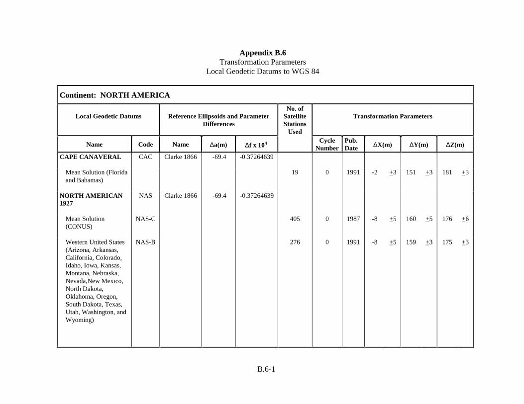
Appendix B.6Transformation Parameters
Local Geodetic Datums to WGS 84
Continent: NORTH AMERICA
Local Geodetic Datums Reference Ellipsoids and ParameterDifferences
No. ofSatelliteStations
Used
Transformation Parameters
Name Code Name ∆a(m) ∆f x 104 Cycle
NumberPub.Date ∆X(m) ∆Y(m) ∆Z(m)
CAPE CANAVERAL CAC Clarke 1866 -69.4 -0.37264639
Mean Solution (Floridaand Bahamas)
19 0 1991 -2 +3 151 +3 181 +3
NORTH AMERICAN1927
NAS Clarke 1866 -69.4 -0.37264639
Mean Solution(CONUS)
NAS-C 405 0 1987 -8 +5 160 +5 176 +6
Western United States(Arizona, Arkansas,California, Colorado,Idaho, Iowa, Kansas,Montana, Nebraska,Nevada,New Mexico,North Dakota,Oklahoma, Oregon,South Dakota, Texas,Utah, Washington, andWyoming)
NAS-B 276 0 1991 -8 +5 159 +3 175 +3
B.6-1

Appendix B.6Transformation Parameters
Local Geodetic Datums to WGS 84
Continent: NORTH AMERICA
Local Geodetic Datums Reference Ellipsoids and ParameterDifferences
No. ofSatelliteStations
Used
Transformation Parameters
Name Code Name ∆a(m) ∆f x 104 Cycle
NumberPub.Date ∆X(m) ∆Y(m) ∆Z(m)
NORTH AMERICAN1927 (cont’d)
NAS Clarke 1866 -69.4 -0.37264639
Eastern United States(Alabama, Connecticut,Delaware, District ofColumbia, Florida,Georgia, Illinois,Indiana, Kentucky,Louisiana, Maine,Maryland,Massachusetts,Michigan, Minnesota,Mississippi, Missouri,New Hampshire, NewJersey, New York,North Carolina, Ohio,Pennsylvania, RhodeIsland, South Carolina,Tennessee, Vermont,Virginia, WestVirginia, andWisconsin)
NAS-A 129 0 1991 -9 +5 161 +5 179 +8
B.6-2

Appendix B.6Transformation Parameters
Local Geodetic Datums to WGS 84
Continent: NORTH AMERICA
Local Geodetic Datums Reference Ellipsoids and ParameterDifferences
No. ofSatelliteStations
Used
Transformation Parameters
Name Code Name ∆a(m) ∆f x 104 Cycle
NumberPub.Date ∆X(m) ∆Y(m) ∆Z(m)
NORTH AMERICAN1927 (cont’d)
NAS Clarke 1866 -69.4 -0.37264639
Alaska (ExcludingAleutian Islands)
NAS-D 47 0 1987 -5 +5 135 +9 172 +5
Aleutian Islands
East of 180°W NAS-V 6 0 1993 -2 +6 152 +8 149 +10
West of 180°W NAS-W 5 0 1993 2 +10204 +10 105 +10
Bahamas(ExcludingSan Salvador Island)
NAS-Q 11 0 1987 -4 +5 154 +3 178 +5
San Salvador Island NAS-R 1 0 1987 1 +25140 +25 165 +25
Canada Mean Solution(IncludingNewfoundland)
NAS-E 112 0 1987 -10 +15 158 +11 187 +6
Alberta and BritishColumbia
NAS-F 25 0 1991 -7 +8 162 +8 188 +6
B.6-3

Appendix B.6Transformation Parameters
Local Geodetic Datums to WGS 84
Continent: NORTH AMERICA
Local Geodetic Datums Reference Ellipsoids and ParameterDifferences
No. ofSatelliteStations
Used
Transformation Parameters
Name Code Name ∆a(m) ∆f x 104 Cycle
NumberPub.Date ∆X(m) ∆Y(m) ∆Z(m)
NORTH AMERICAN1927 (cont’d)
NAS Clarke 1866 -69.4 -0.37264639
Eastern Canada(Newfoundland, NewBrunswick, NovaScotia, and Quebec)
NAS-G 37 0 1991 -22 +6 160 +6 190 +3
Manitoba and Ontario NAS-H 25 0 1991 -9 +9 157 +5 184 +5
Northwest Territoriesand Saskatchewan
NAS-I 17 0 1991 4 +5 159 +5 188 +3
Yukon NAS-J 8 0 1991 -7 +5 139 +8 181 +3
Canal Zone NAS-O 3 0 1987 0 +20 125 +20 201 +20
Caribbean (AntiguaIsland, Barbados,Barbuda, CaicosIslands, Cuba,Dominican Republic,Grand Cayman,Jamaica, and TurksIslands)
NAS-P 15 0 1991 -3 +3 142 +9 183 +12
B.6-4

Appendix B.6Transformation Parameters
Local Geodetic Datums to WGS 84
Continent: NORTH AMERICA
Local Geodetic Datums Reference Ellipsoids and ParameterDifferences
No. ofSatelliteStations
Used
Transformation Parameters
Name Code Name ∆a(m) ∆f x 104 Cycle
NumberPub.Date ∆X(m) ∆Y(m) ∆Z(m)
NORTH AMERICAN1927 (cont’d)
NAS Clarke 1866 -69.4 -0.37264639
Central America(Belize, Costa Rica, ElSalvador, Guatemala,Honduras, andNicaragua)
NAS-N 19 0 1987 0 +8 125 +3 194 +5
Cuba NAS-T 1 0 1987 -9 +25 152 +25 178 +25
Greenland(HayesPeninsula)
NAS-U 2 0 1987 11 +25 114 +25 195 +25
Mexico NAS-L 22 0 1987 -12 +8 130 +6 190 +6
NORTH AMERICAN1983
NAR GRS 80 0 -0.00000016
Alaska (ExcludingAleutian Islands)
NAR-A 42 0 1987 0 +2 0 +2 0 +2
Aleutian Islands NAR-E 4 0 1993 -2 +5 0 +2 4 +5
Canada NAR-B 96 0 1987 0 +2 0 +2 0 +2
B.6-5

Appendix B.6Transformation Parameters
Local Geodetic Datums to WGS 84
Continent: NORTH AMERICA
Local Geodetic Datums Reference Ellipsoids and ParameterDifferences
No. ofSatelliteStations
Used
Transformation Parameters
Name Code Name ∆a(m) ∆f x 104 Cycle
NumberPub.Date ∆X(m) ∆Y(m) ∆Z(m)
NORTH AMERICAN1983 (cont’d)
NAR GRS 80 0 -0.00000016
CONUS NAR-C 216 0 1987 0 +2 0 +2 0 +2
Hawaii NAR-H 6 0 1993 1 +2 1 +2 -1 +2
Mexico and CentralAmerica
NAR-D 25 0 1987 0 +2 0 +2 0 +2
B.6-6

Appendix B.7Transformation Parameters
Local Geodetic Datums to WGS 84
Continent: SOUTH AMERICA
Local Geodetic Datums Reference Ellipsoids and ParameterDifferences
No. ofSatelliteStations
Used
Transformation Parameters
Name Code Name ∆a(m) ∆f x 104 Cycle
NumberPub.Date ∆X(m) ∆Y(m) ∆Z(m)
BOGOTAOBSERVATORY
BOO International1924
-251 -0.14192702
Colombia 7 0 1987 307 +6 304 +5 -318 +6
CAMPO INCHAUSPE1969
CAI International1924
-251 -0.14192702
Argentina 20 0 1987 -148 +5 136 +5 90 +5
CHUA ASTRO CHU International1924
-251 -0.14192702
Paraguay 6 0 1987 -134 +6 229 +9 -29 +5
CORREGO ALEGRE COA International1924
-251 -0.14192702
Brazil 17 0 1987 -206 +5 172 +3 -6 +5
B.7-1

Appendix B.7Transformation Parameters
Local Geodetic Datums to WGS 84
Continent: SOUTH AMERICA
Local Geodetic Datums Reference Ellipsoids and ParameterDifferences
No. ofSatelliteStations
Used
Transformation Parameters
Name Code Name ∆a(m) ∆f x 104 Cycle
NumberPub.Date ∆X(m) ∆Y(m) ∆Z(m)
PROVISIONALSOUTH AMERICAN1956
PRP International1924
-251 -0.14192702
Mean Solution(Bolivia, Chile,Colombia, Ecuador,Guyana, Peru, andVenezuela)
PRP-M 63 0 1987 -288 +17 175 +27 -376 -27
Bolivia PRP-A 5 0 1991 -270 +5 188 +11 -388 +14
Chile
Northern Chile (near19°S)
PRP-B 1 0 1991 -270 +25 183 +25 -390 +25
Southern Chile (near43°S)
PRP-C 3 0 1991 -305 +20 243 +20 -442 +20
Colombia PRP-D 4 0 1991 -282 +15169 +15 -371 +15
Ecuador PRP-E 11 0 1991 -278 +3171 +5 -367 +3
B.7-2

Appendix B.7Transformation Parameters
Local Geodetic Datums to WGS 84
Continent: SOUTH AMERICA
Local Geodetic Datums Reference Ellipsoids and ParameterDifferences
No. ofSatelliteStations
Used
Transformation Parameters
Name Code Name ∆a(m) ∆f x 104 Cycle
NumberPub.Date ∆X(m) ∆Y(m) ∆Z(m)
PROVISIONALSOUTH AMERICAN1956 (cont’d)
PRP International1924
-251 -0.14192702
Guyana PRP-F 9 0 1991 -298 +6 159 +14 -369 -+5
Peru PRP-G 6 0 1991 -279 +6 175 +8 -379 +12
Venezuela PRP-H 24 0 1991 -295 -+9 173 +14 -371 +15
PROVISIONALSOUTH CHILEAN1963*
HIT International1924
-251 -0.14192702
Southern Chile (near53°S)
2 0 1987 16 +25 196 +25 93 +25
* Also known as Hito XVIII 1963
B.7-3

Appendix B.7Transformation Parameters
Local Geodetic Datums to WGS 84
Continent: SOUTH AMERICA
Local Geodetic Datums Reference Ellipsoids and ParameterDifferences
No. ofSatelliteStations
Used
Transformation Parameters
Name Code Name ∆a(m) ∆f x 104 Cycle
NumberPub.Date ∆X(m) ∆Y(m) ∆Z(m)
SOUTH AMERICAN1969
SAN SouthAmerican
1969
-23 -0.00081204
MeanSolution(Argentina,Bolivia, Brazil, Chile,Colombia, Ecuador,Guyana, Paraguay,Peru, Trinidad andTobago, andVenezuela)
SAN-M 84 0 1987 -57 +15 1 +6 -41 +9
Argentina SAN-A 10 0 1991 -62 +5 -1 +5 -37 +5
Bolivia SAN-B 4 0 1991 -61 +15 2 +15 -48 +15
Brazil SAN-C 22 0 1991 -60 +3 -2 +5 -41 +5
Chile SAN-D 9 0 1991 -75 +15 -1 +8 -44 +11
Colombia SAN-E 7 0 1991 -44 +6 6 +6 -36 +5
B.7-4

Appendix B.7Transformation Parameters
Local Geodetic Datums to WGS 84
Continent: SOUTH AMERICA
Local Geodetic Datums Reference Ellipsoids and ParameterDifferences
No. ofSatelliteStations
Used
Transformation Parameters
Name Code Name ∆a(m) ∆f x 104 Cycle
NumberPub.Date ∆X(m) ∆Y(m) ∆Z(m)
SOUTH AMERICAN1969 (cont’d)
SAN SouthAmerican
1969
-23 -0.00081204
Ecuador (ExcludingGalapagos Islands)
SAN-F 11 0 1991 -48 +3 3 +3 -44 +3
Baltra, GalapagosIslands
SAN-J 1 0 1991 -47 +25 26 +25 -42 +25
Guyana SAN-G 5 0 1991 -53 +9 3 +5 -47 +5
Paraguay SAN-H 4 0 1991 -61 +15 2 +15 -33 +15
Peru SAN-I 6 0 1991 -58 +5 0 +5 -44 +5
Trinidad and Tobago SAN-K 1 0 1991 -45 +25 12 +25 -33 +25
Venezuela SAN-L 5 0 1991 -45 +3 8 +6 -33 +3
ZANDERIJ ZAN International1924
-251 -0.14192702
Suriname 5 0 1987 -265 +5 120 +5 -358 +8
B.7-5

Appendix B.8Transformation Parameters
Local Geodetic Datums to WGS 84
Continent: ATLANTIC OCEAN
Local Geodetic Datums Reference Ellipsoids and ParameterDifferences
No. ofSatelliteStations
Used
Transformation Parameters
Name Code Name ∆a(m) ∆f x 104 Cycle
NumberPub.Date ∆X(m) ∆Y(m) ∆Z(m)
ANTIGUA ISLANDASTRO 1943
AIA Clarke 1880 -112.145 -0.54750714
Antigua, LeewardIslands
1 0 1991 -270 +25 13 +25 62 +25
ASCENSION ISLAND1958
ASC International1924
-251 -0.14192702
Ascension Island 2 0 1991 -205 +25 107 +25 53 +25
ASTRO DOS 71/4 SHB International1924
-251 -0.14192702
St. Helena Island 1 0 1987 -320 +25 550 +25 -494 +25
BERMUDA 1957 BER Clarke 1866 -69.4 -0.37264639
Bermuda Islands 3 0 1987 -73 +20 213 +20 296 +20
CAPE CANAVERAL CAC Clarke 1866 -69.4 -0.37264639
Mean Solution(Bahamas and Florida)
19 0 1991 -2 +3 151 +3 181 +3
B.8-1
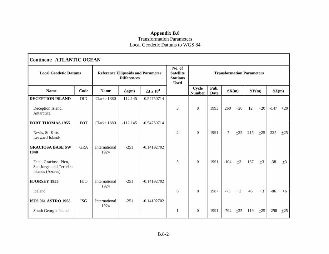
Appendix B.8Transformation Parameters
Local Geodetic Datums to WGS 84
Continent: ATLANTIC OCEAN
Local Geodetic Datums Reference Ellipsoids and ParameterDifferences
No. ofSatelliteStations
Used
Transformation Parameters
Name Code Name ∆a(m) ∆f x 104 Cycle
NumberPub.Date ∆X(m) ∆Y(m) ∆Z(m)
DECEPTION ISLAND DID Clarke 1880 -112.145 -0.54750714
Deception Island,Antarctica
3 0 1993 260 +20 12 +20 -147 +20
FORT THOMAS 1955 FOT Clarke 1880 -112.145 -0.54750714
Nevis, St. Kitts,Leeward Islands
2 0 1991 -7 +25 215 +25 225 +25
GRACIOSA BASE SW1948
GRA International1924
-251 -0.14192702
Faial, Graciosa, Pico,Sao Jorge, and TerceiraIslands (Azores)
5 0 1991 -104 +3 167 +3 -38 +3
HJORSEY 1955 HJO International1924
-251 -0.14192702
Iceland 6 0 1987 -73 +3 46 +3 -86 +6
ISTS 061 ASTRO 1968 ISG International1924
-251 -0.14192702
South Georgia Island 1 0 1991 -794 +25 119 +25 -298 +25
B.8-2

Appendix B.8Transformation Parameters
Local Geodetic Datums to WGS 84
Continent: ATLANTIC OCEAN
Local Geodetic Datums Reference Ellipsoids and ParameterDifferences
No. ofSatelliteStations
Used
Transformation Parameters
Name Code Name ∆a(m) ∆f x 104 Cycle
NumberPub.Date ∆X(m) ∆Y(m) ∆Z(m)
L. C. 5 ASTRO 1961 LCF Clarke 1866 -69.4 -0.37264639
Cayman Brac Island 1 0 1987 42 +25 124 +25 147 +25
MONTSERRATISLAND ASTRO 1958
ASM Clarke 1880 -112.145 -0.54750714
Montserrat, LeewardIslands
1 0 1991 174 +25 359 +25 365 +25
NAPARIMA, BWI NAP International1924
-251 -0.14192702
Trinidad and Tobago 4 0 1991 -10 +15 375 +15 165 +15
OBSERVATORIOMETEOROLOGICO1939
FLO International1924
-251 -0.14192702
Corvo and FloresIslands (Azores)
3 0 1991 -425 +20 -169 +20 81 +20
PICO DE LAS NIEVES PLN International1924
-251 -0.14192702
Canary lslands 1 0 1987 -307 +25 -92 +25 127 +25
B.8-3

Appendix B.8Transformation Parameters
Local Geodetic Datums to WGS 84
Continent: ATLANTIC OCEAN
Local Geodetic Datums Reference Ellipsoids and ParameterDifferences
No. ofSatelliteStations
Used
Transformation Parameters
Name Code Name ∆a(m) ∆f x 104 Cycle
NumberPub.Date ∆X(m) ∆Y(m) ∆Z(m)
PORTO SANTO 1936 POS International1924
-251 -0.14192702
Porto Santo andMadeira Islands
2 0 1991 -499 +25 -249 +25 314 +25
PUERTO RICO PUR Clarke 1866 -69.4 -0.37264639
Puerto Rico and VirginIslands
11 0 1987 11 +3 72 +3 -101 +3
QORNOQ QUO International1924
-251 -0.14192702
South Greenland 2 0 1987 164 +25 138 +25 -189 +32
SAO BRAZ SAO International1924
-251 -0.14192702
Sao Miguel, SantaMaria Islands (Azores)
2 0 1987 -203 +25 141 +25 53 +25
SAPPER HILL 1943 SAP International1924
-251 -0.14192702
East Falkland Island 5 0 1991 -355 +1 21 +1 72 +1
B.8-4

Appendix B.8Transformation Parameters
Local Geodetic Datums to WGS 84
Continent: ATLANTIC OCEAN
Local Geodetic Datums Reference Ellipsoids and ParameterDifferences
No. ofSatelliteStations
Used
Transformation Parameters
Name Code Name ∆a(m) ∆f x 104 Cycle
NumberPub.Date ∆X(m) ∆Y(m) ∆Z(m)
SELVAGEM GRANDE1938
SGM International1924
-251 -0.14192702
Salvage Islands 1 0 1991 -289 +25 -124 +25 60 +25
TRISTAN ASTRO 1968 TDC International1924
-251 -0.14192702
Tristan da Cunha 1 0 1987 -632 +25 438 +25 -609 +25
B.8-5

Appendix B.9Transformation Parameters
Local Geodetic Datums to WGS 84
Continent: Indian Ocean
Local Geodetic Datums Reference Ellipsoids and ParameterDifferences
No. ofSatelliteStations
Used
Transformation Parameters
Name Code Name ∆a(m) ∆f x 104 Cycle
NumberPub.Date ∆X(m) ∆Y(m) ∆Z(m)
ANNA 1 ASTRO 1965 ANO AustralianNational
-23 -0.00081204
Cocos Islands 1 0 1987 -491 +25 -22 +25 435 +25
GAN 1970 GAA International1924
-251 -0.14192702
Republic of Maldives 1 0 1987 -133 +25 -321 +25 50 +25
ISTS 073 ASTRO 1969 IST International1924
-251 -0.14192702
Diego Garcia 2 0 1987 208 +25 -435 +25 -229 +25
KERGUELEN ISLAND1949
KEG International1924
-251 -0.14192702
Kerguelen Island 1 0 1987 145 +25 -187 +25 103 +25
MAHE 1971 MIK Clarke 1880 -112.145 -0.54750714
Mahe Island 1 0 1987 41 +25 -220 +25 -134 +25
REUNION REU International1924
-251 -0.14192702
Mascarene Islands 1 0 1987 94 +25 -948 +25 -1262 +25
B.9-1
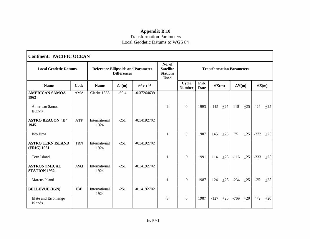
Appendix B.10Transformation Parameters
Local Geodetic Datums to WGS 84
Continent: PACIFIC OCEAN
Local Geodetic Datums Reference Ellipsoids and ParameterDifferences
No. ofSatelliteStations
Used
Transformation Parameters
Name Code Name ∆a(m) ∆f x 104 Cycle
NumberPub.Date ∆X(m) ∆Y(m) ∆Z(m)
AMERICAN SAMOA1962
AMA Clarke 1866 -69.4 -0.37264639
American SamoaIslands
2 0 1993 -115 +25 118 +25 426 +25
ASTRO BEACON "E"1945
ATF International1924
-251 -0.14192702
Iwo Jima 1 0 1987 145 +25 75 +25 -272 +25
ASTRO TERN ISLAND(FRIG) 1961
TRN International1924
-251 -0.14192702
Tern Island 1 0 1991 114 +25 -116 +25 -333 +25
ASTRONOMICALSTATION 1952
ASQ International1924
-251 -0.14192702
Marcus Island 1 0 1987 124 +25 -234 +25 -25 +25
BELLEVUE (IGN) IBE International1924
-251 -0.14192702
Efate and ErromangoIslands
3 0 1987 -127 +20 -769 +20 472 +20
B.10-1

Appendix B.10Transformation Parameters
Local Geodetic Datums to WGS 84
Continent: PACIFIC OCEAN
Local Geodetic Datums Reference Ellipsoids and ParameterDifferences
No. ofSatelliteStations
Used
Transformation Parameters
Name Code Name ∆a(m) ∆f x 104 Cycle
NumberPub.Date ∆X(m) ∆Y(m) ∆Z(m)
CANTON ASTRO 1966 CAO International1924
-251 -0.14192702
Phoenix Islands 4 0 1987 298 +15 -304 +15 -375 +15
CHATHAM ISLANDASTRO 1971
CHI International1924
-251 -0.14192702
Chatham Island (NewZealand)
4 0 1987 175 +15 -38 +15 113 +15
DOS 1968 GIZ International1924
-251 -0.14192702
Gizo Island (NewGeorgia Islands)
1 0 1987 230 +25 -199 +25 -752 +25
EASTER ISLAND 1967 EAS International1924
-251 -0.14192702
Easter Island 1 0 1987 211 +25 147 +25 111 +25
GEODETIC DATUM1949
GEO International1924
-251 -0.14192702
New Zealand 14 0 1987 84 +5 -22 +3 209 +5
B.10-2

Appendix B.10Transformation Parameters
Local Geodetic Datums to WGS 84
Continent: PACIFIC OCEAN
Local Geodetic Datums Reference Ellipsoids and ParameterDifferences
No. ofSatelliteStations
Used
Transformation Parameters
Name Code Name ∆a(m) ∆f x 104 Cycle
NumberPub.Date ∆X(m) ∆Y(m) ∆Z(m)
GUAM 1963 GUA Clarke 1866 -69.4 -0.37264639
Guam 5 0 1987 -100 +3 -248 +3 259 +3
GUX l ASTRO DOB International1924
-251 -0.14192702
Guadalcanal Island 1 0 1987 252 +25 -209 +25 -751 +25
INDONESIAN 1974 IDN Indonesian1974
-23 -0.00114930
Indonesia 1 0 1993 -24 +25 -15 +25 5 +25
JOHNSTON ISLAND1961
JOH International1924
-251 -0.14192702
Johnston Island 2 0 1991 189 +25 -79 +25 -202 +25
KUSAIE ASTRO 1951 KUS International1924
-251 -0.14192702
Caroline Islands, Fed.States of Micronesia
1 0 1991 647 +25 1777 +25 -1124 +25
B.10-3

Appendix B.10Transformation Parameters
Local Geodetic Datums to WGS 84
Continent: PACIFIC OCEAN
Local Geodetic Datums Reference Ellipsoids and ParameterDifferences
No. ofSatelliteStations
Used
Transformation Parameters
Name Code Name ∆a(m) ∆f x 104 Cycle
NumberPub.Date ∆X(m) ∆Y(m) ∆Z(m)
LUZON LUZ Clarke 1866 -69.4 -0.37264639
Philippines (ExcludingMindanao Island)
LUZ-A 6 0 1987 -133 +8 -77 +11 -51 +9
Mindanao Island LUZ-B 1 0 1987 -133 +25 -79 +25 -72 +25
MIDWAY ASTRO 1961 MID International1924
-251 -0.14192702
Midway Islands 1 0 1987 912 +25 -58 +25 1227 +25
OLD HAWAIIAN OHA Clarke 1866 -69.4 -0.37264639
Mean Solution OHA-M 15 0 1987 61 +25 -285 +20 -181 +20
Hawaii OHA-A 2 0 1991 89 +25 -279 +25 -183 +25
Kauai OHA-B 3 0 1991 45 +20 -290 +20 -172 +20
Maui OHA-C 2 0 1991 65 +25 -290 +25 -190 +25
Oahu OHA-D 8 0 1991 58 +10 -283 +6 -182 +6
B.10-4

Appendix B.10Transformation Parameters
Local Geodetic Datums to WGS 84
Continent: PACIFIC OCEAN
Local Geodetic Datums Reference Ellipsoids and ParameterDifferences
No. ofSatelliteStations
Used
Transformation Parameters
Name Code Name ∆a(m) ∆f x 104 Cycle
NumberPub.Date ∆X(m) ∆Y(m) ∆Z(m)
PITCAIRN ASTRO1967
PIT International1924
-251 -0.14192702
Pitcairn Island 1 0 1987 185 +25 165 +25 42 +25
SANTO (DOS) 1965 SAE International1924
-251 -0.14192702
Espirito Santo Island 1 0 1987 170 +25 42 +25 84 +25
VITI LEVU 1916 MVS Clarke 1880 -112.145 -0.54750714
Viti Levu Island (FijiIslands)
1 0 1987 51 +25 391 +25 -36 +25
WAKE-ENIWETOK1960
ENW Hough -133 -0.14192702
Marshall Islands 10 0 1991 102 +3 52 +3 -38 +3
WAKE ISLANDASTRO 1952
WAK International1924
-251 -0.14192702
Wake Atoll 2 0 1991 276 +25 -57 +25 149 +25
B.10-5

C-1
APPENDIX C
DATUM TRANSFORMATIONS DERIVED
USING NON-SATELLITE INFORMATION

C-2
This page is intentionally left blank

C-3
DATUM TRANSFORMATION CONSTANTSLOCAL GEODETIC DATUMS TO WGS 84
(THROUGH NON-SATELLITE TIES)
1. GENERAL
This appendix provides the details about the reference ellipsoids (Appendix A) usedas defining parameters for the local geodetic datums which are related to WGS 84through non-satellite ties to the local control.
There are ten such local/regional geodetic datums, and one special area under theEuropean Datum 1950 (ED 50).
2. LOCAL DATUM ELLIPSOIDS
Appendix C.1 lists alphabetically the local geodetic datums and their associatedellipsoids. Two letter ellipsoidal codes (Appendix A) have also been included to clearlyindicate which "version" of the ellipsoid has been used to determine the transformationconstants.
3. TRANSFORMATION CONSTANTS
Appendix C.2 alphabetically lists the local geodetic datums and the special areaunder ED 50 with the associated shift constants.
The year of initial publication and cycle numbers have been provided as a newfeature in this edition. This makes it possible for a user to determine when a particular setof transformation parameters first became available and if the current set has replaced anoutdated set.
A cycle number of zero indicates that the set of parameters are as they werepublished in DMA TR 8350.2, Second Edition, 1 September 1991 including Insert 1,30 August 1993 or that the parameters are new to this edition (1997 Publication Date). Acycle number of one indicates that the current parameters have replaced outdatedparameters that were in the previous edition.
If transformation parameter sets are updated in future editions of this publication,the cycle numbers for each parameter set that is updated will increment by one.
4. ERROR ESTIMATES
The error estimates are not available for the datum transformation constants listedin the Appendix C.2.

C-4
This page is intentionally left blank

* See Appendix A.1 for associated constants a,f.
C.1-1
Appendix C.1Local Geodetic Datums
Related to World Geodetic System 1984(Through non-Satellite Ties)
Local Geodetic DatumAssociated*
Reference Ellipsoid CodeBukit Rimpah Bessel 1841 BRCamp Area Astro International 1924 INEuropean 1950 International 1924 INGunung Segara Bessel 1841 BRHerat North International 1924 INHermannskogel Bessel 1841 BRIndian Everest EFPulkovo 1942 Krassovsky 1940 KATananarive Observatory 1925 International 1924 INVoirol 1874 Clarke 1880 CDYacare International 1924 IN

C.1-2
This page is intentionally left blank

Appendix C.2Non-Satellite Derived Transformation Parameters
Local Geodetic Datums to WGS 84
Local Geodetic DatumsReference Ellipsoids and Parameter
Differences Transformation Parameters
Name Code Name ∆a(m) ∆f x 104 CycleNumber Pub. Date ∆X(m) ∆Y(m) ∆Z(m)
BUKIT RIMPAH BUR Bessel 1841 739.845 0.10037483
Bangka and BelitungIslands (Indonesia)
0 1987 -384 664 -48
CAMP AREA ASTRO CAZ International 1924 -251 -0.14192702
Camp McMurdo Area,Antarctica
0 1987 -104 -129 239
EUROPEAN 1950 EUR-S International 1924 -251 -0.14192702
Iraq, Israel, JordanKuwait, Lebanon, SaudiArabia, and Syria
0 1991 -103 -106 -141
GUNUNG SEGARA GSE Bessel 1841 739.845 0.10037483
Kalimantan (Indonesia) 0 1987 -403 684 41
HERAT NORTH HEN International 1924 -251 -0.14192702
Afghanistan 0 1987 -333 -222 114
C.2-1

Appendix C.2Non-Satellite Derived Transformation Parameters
Local Geodetic Datums to WGS 84
Local Geodetic DatumsReference Ellipsoids and Parameter
Differences Transformation Parameters
Name Code Name ∆a(m) ∆f x 104 CycleNumber Pub. Date ∆X(m) ∆Y(m) ∆Z(m)
HERMANNSKOGEL HER Bessel 1841 739.845 0.10037483
Yugoslavia (Prior to1990) Slovenia, Croatia,Bosnia and Herzegovina,Serbia
0 1997 682 -203 480
INDIAN IND-P Everest 827.387* 0.28361368
Pakistan 0 1993 283 682 231
PULKOVO 1942 PUK Krassovsky 1940 -108 0.00480795
Russia 0 1993 28 -130 -95
TANANARIVEOBSERVATORY 1925
TAN International 1924 -251 -0.14192702
Madagascar 0 1987 -189 -242 -91
VOIROL 1874 VOI Clarke 1880 -112.145 -0.54750714
Tunisia/Algeria 0 1997 -73 -247 227
YACARE YAC International 1924 -251 -0.14192702
Uruguay 0 1987 -155 171 37
* See Appendix A.1
C.2-2

D-1
APPENDIX D
MULTIPLE REGRESSION EQUATIONS FORSPECIAL CONTINENTAL SIZELOCAL GEODETIC DATUMS

D-2
This page is intentionally blank.

D-3
MULTIPLE REGRESSION EQUATIONS
1. GENERAL
This appendix provides the Multiple Regression Equations (MREs) parameters forcontinental size datums and for contiguous large land areas (Table D-1).
Table D.1
DATUMS WITH MULTIPLE REGRESSION EQUATIONS
DATUM NAME AREA COVEREDAustralian Geodetic 1966 Australian MainlandAustralian Geodetic 1984 Australian MainlandCampo Inchauspe ArgentinaCorrego Alegre BrazilEuropean 1950 Western Europe (Austria, Denmark, France,
W. Germany*, The Netherlands, andSwitzerland.)
North American 1927 CONUS and Canadian MainlandSouth American 1969 South American Mainland (Argentina, Bolivia,
Brazil, Chile, Colombia, Ecuador, Guyana,Peru, Paraguay, Uruguay, and Venezuela.
* Prior to October 1990.
2. APPLICATIONS
The coverage area for MREs application are defined in detail for each datum.MREs coverage area should never be extrapolated and are not to be used over islandsand/or isolated land areas.
The main advantage of MREs lies in their modeling of distortions for datums,which cover continental size land areas, to obtain better transformation fit in geodeticapplications.

D-4
This page is intentionally blank.

D-5
Multiple Regression Equations (MREs)for Transforming
Australian Geodetic Datum 1966 (AUA) to WGS 84
Area of Applicability : Australian Mainland (excluding Tasmania)
MRE coefficients for ø and λ are :
∆ø" = 5.19238 + 0.12666 U + 0.52309 V - 0.42069 U2 - 0.39326 UV + 0.93484 U2V+ 0.44249 UV2 - 0.30074 UV3 + 1.00092 U5 - 0.07565 V6 - 1.42988 U9
- 16.06639 U4V5 + 0.07428 V9 + 0.24256 UV9 + 38.27946 U6V7
- 62.06403 U7V8 + 89.19184 U9V8
∆λ" = 4.69250 - 0.87138 U - 0.50104 V + 0.12678 UV - 0.23076 V2 - 0.61098 U2V- 0.38064 V3 + 2.89189 U6 + 5.26013 U2V5 - 2.97897 U8 + 5.43221 U3V5
- 3.40748 U2V6 + 0.07772 V8 + 1.08514 U8V + 0.71516 UV8 + 0.20185 V9
+ 5.18012 U2V8 - 1.72907 U3V8 - 1.24329 U2V 9
Where : U = K (ø + 27°); V = K (λ - 134°); K = 0.05235988
NOTE : Input ø as (-) from 90°S to 0°N in degrees.
Input λ as (-) from 180°W to 0°E in degrees.
Quality of fit = ± 2.0 m
Test Case :
AUA Shift WGS 84
ø = (-)17° 00' 32.78"S ∆ø = 5.48" ø = (-)17° 00' 27.30"Sλ = 144° 11' 37.25"E∆λ = 3.92" λ = 144° 11' 41.17"E

D-6
Multiple Regression Equations (MREs)for Transforming
Australian Geodetic Datum 1984 (AUG) to WGS 84
Area of Applicability : Australian Mainland (excluding Tasmania)
MRE coefficients for ø and λ are :
∆ø" = 5.20604 + 0.25225 U + 0.58528 V - 0.41584 U2 - 0.38620 UV - 0.06820 V2
+ 0.38699 U2V + 0.07934 UV2 + 0.37714 U4 - 0.52913 U4V + 0.38095 V7
+ 0.68776 U2V6 - 0.03785 V8 - 0.17891 U9 - 4.84581 U2V7 - 0.35777 V9
+ 4.23859 U2V9
∆λ" = 4.67877 - 0.73036 U - 0.57942 V + 0.28840 U2 + 0.10194 U3 - 0.27814 UV2
- 0.13598 V3 + 0.34670 UV3 - 0.46107 V4 + 1.29432 U2V3 + 0.17996 UV4
- 1.13008 U2V5 - 0.46832 U8 + 0.30676 V8 + 0.31948 U9 + 0.16735 V9
- 1.19443 U3V9
Where : U = K (ø + 27°); V = K (λ - 134°); K = 0.05235988
NOTE : Input ø as (-) from 90°S to 0°N in degrees.
Input λ as (-) from 180°W to 0°E in degrees.
Quality of fit = ± 2.0 m
Test Case :
AUG Shift WGS 84
ø = (-)20° 38' 00.67"S ∆ø = 5.50" ø = (-)20° 37' 55.17"Sλ = 144° 24' 29.29"E∆λ = 4.11" λ = 144° 24' 33.40"E

D-7
Multiple Regression Equations (MREs)for Transforming
Campo Inchauspe Datum (CAI) to WGS 84
Area of Applicability : Argentina (Continental land areas only)
MRE coefficients for ø and λ are :
∆ø" = 1.67470 + 0.52924 U - 0.17100 V + 0.18962 U2 + 0.04216 UV + 0.19709 UV2
- 0.22037 U4 - 0.15483 U2V2 - 0.24506 UV4 - 0.05675 V5 + 0.06674 U6
+ 0.01701 UV5 - 0.00202 U7 + 0.08625 V7 - 0.00628 U8 + 0.00172 U8V4
+ 0.00036 U9V6
∆λ" = - 2.93117 + 0.18225 U + 0.69396 V - 0.04403 U2 + 0.07955 V2 + 1.48605 V3
- 0.00499 U4 - 0.02180 U4V - 0.29575 U2V3 + 0.20377 UV4 - 2.47151 V5
+ 0.09073 U3V4 + 1.33556 V7 + 0.01575 U3V5 - 0.26842 V9
Where : U = K ( ø + 35°); V = K ( λ + 64°); K = 0.15707963
NOTE : Input ø as (-) from 90°S to 0°N in degrees.
Input λ as (-) from 180°W to 0°E in degrees.
Quality of fit = ± 2.0 m
Test Case :
CAI Shift WGS 84
ø = (-)29° 47' 45.68"S ∆ø = 1.95" ø = (-)29° 47' 43.73"Sλ = (-)58° 07' 38.20"W ∆λ =-1.96" λ = (-)58° 07' 40.16"W

D-8
Multiple Regression Equations (MREs)for Transforming
Corrego Alegre Datum (COA) to WGS 84
Area of Applicability : Brazil (Continental land areas only)
MRE coefficients for ø and λ are :
∆ø" = - 0.84315 + 0.74089 U - 0.21968 V - 0.98875 U2 + 0.89883 UV + 0.42853 U3
+ 2.73442 U4 - 0.34750 U3V + 4.69235 U2V 3 - 1.87277 U6 + 11.06672 U5V- 46.24841 U3V3 - 0.92268 U7 - 14.26289 U7V + 334.33740 U5V5
- 15.68277 U9V2 - 2428.8586 U8V8
∆λ" = - 1.46053 + 0.63715 U + 2.24996 V - 5.66052 UV + 2.22589 V2 - 0.34504 U3
- 8.54151 U2V + 0.87138 U4 + 43.40004 U3V + 4.35977 UV3 + 8.17101 U4V+ 16.24298 U2V3 + 19.96900 UV4 - 8.75655 V5 - 125.35753 U5V- 127.41019 U3V4 - 0.61047 U8 + 138.76072 U7V + 122.04261 U5V4
- 51.86666 U9V + 45.67574 U9V3
Where : U = K ( ø + 15°); V = K ( λ + 50°); K = 0.05235988
NOTE : Input ø as (-) from 90°S to 0°N in degrees.
Input λ as (-) from 180°W to 0°E in degrees.
Quality of fit = ± 2.0 m
Test Case :
COA Shift WGS 84
ø = (-)20° 29' 01.02"S ∆ø = -1.03" ø = (-)20° 29' 02.05"Sλ = (-)54° 47' 13.17"W ∆λ = -2.10" λ = (-)54° 47' 15.27"W

D-9
Multiple Regression Equations (MREs)for Transforming
European Datum 1950 (EUR) to WGS 84
Area of Applicability : Western Europe* (Continental contiguous land areas only)
MRE coefficients for ø and λ are :
∆ø" = - 2.65261 + 2.06392 U + 0.77921 V + 0.26743 U2 + 0.10706 UV + 0.76407 U3
- 0.95430 U2V + 0.17197 U4 + 1.04974 U4V - 0.22899 U5V2 - 0.05401 V8
- 0.78909 U9 - 0.10572 U2V7 + 0.05283 UV9 + 0.02445 U3V9
∆λ" = - 4.13447 - 1.50572 U + 1.94075 V - 1.37600 U2 + 1.98425 UV + 0.30068 V2
- 2.31939 U3 - 1.70401 U4 - 5.48711 UV3 + 7.41956 U5 - 1.61351 U2V3
+ 5.92923 UV4 - 1.97974 V5 + 1.57701 U6 - 6.52522 U3V 3 + 16.85976 U2V4
- 1.79701 UV5 - 3.08344 U7 - 14.32516 U6V + 4.49096 U4V4 + 9.98750 U8V+ 7.80215 U7V2 - 2.26917 U2V7 + 0.16438 V9 - 17.45428 U4V6 - 8.25844 U9V2 + 5.28734 U8V3 + 8.87141 U5V7 - 3.48015 U9V4 + 0.71041 U4V 9
Where : U = K ( ø - 52°); V = K ( λ - 10°); K = 0.05235988
NOTE Input ø as (-) from 90°S to 0°N in degrees.
Input λ as (-) from 180°W to 0°E in degrees.
Quality of fit = ± 2.0 m
Test Case :
EUR Shift WGS 84
ø = 46° 41' 42.89"N ∆ø = -3.08" ø = 46° 41' 39.81"Nλ = 13° 54' 54.09"E ∆λ = -3.49" λ = 13° 54' 50.60"E
* See Table D.1 (Page D-3) for the list of countries covered by the above set of MREs.

D-10
Multiple Regression Equations (MREs)for Transforming
North American Datum 1927 (NAS) to WGS 84
Area of Applicability : Canada (Continental contiguous land areas only)
MRE coefficients for ø and λ are :
∆ø" = 0.79395 + 2.29199 U + 0.27589 V - 1.76644 U2 + 0.47743 UV + 0.08421 V2
- 6.03894 U3 - 3.55747 U2V - 1.81118 UV2 - 0.20307 V3 + 7.75815 U4
- 3.1017 U3V + 3.58363 U2V2 - 1.31086 UV3 - 0.45916 V4 + 14.27239 U5
+ 3.28815 U4V + 1.35742 U2V3 + 1.75323 UV4 + 0.44999 V5 - 19.02041 U4V2 - 1.01631 U2V4 + 1.47331 UV5 + 0.15181 V6 + 0.41614 U2V5 - 0.80920 UV6
- 0.18177 V7 + 5.19854 U4V4 - 0.48837 UV7 - 0.01473 V8 - 2.26448 U9
- 0.46457 U2V7 + 0.11259 UV8 + 0.02067 V9 + 47.64961 U8V2 + 0.04828 UV9
+ 36.38963 U9V2 + 0.06991 U4V 7 + 0.08456 U3V8 + 0.09113 U2V9
+ 5.93797 U7V5 - 2.36261 U7V6 + 0.09575 U5V8
∆λ" = - 1.36099 + 3.61796 V - 3.97703 U2 + 3.09705 UV - 1.15866 V2 - 13.28954 U3
- 3.15795 U2V + 0.68405 UV2 - 0.50303 V3 - 8.81200 U3V - 2.17587 U2V2
- 1.49513 UV3 + 0.84700 V4 + 31.42448 U5 - 14.67474 U3V2 + 0.65640 UV4
+ 17.55842 U6 + 6.87058 U4V2 - 0.21565 V6 + 62.18139 U5V2 + 1.78687 U3V4
+ 2.74517 U2V5 - 0.30085 UV6 + 0.04600 V7 + 63.52702 U6V2 + 7.83682 U5V3
+ 9.59444 U3V5 + 0.01480 V8 + 10.51228 U4V5 - 1.42398 U2V7 - 0.00834 V9
+ 5.23485 U7V3 - 3.18129 U3V7 + 8.45704 U9V2 - 2.29333 U4V7
+ 0.14465 U2V9 + 0.29701 U3V9 + 0.17655 U4V9
Where : U = K ( ø - 60°); V = K ( λ + 100°); K = 0.05235988
NOTE : Input ø as (-) from 90°S to 0°N in degrees.
Input λ as (-) from 180°W to 0°E in degrees.
Quality of fit = ± 2.0 m
Test Case :
NAS Shift WGS 84
ø = 54° 26' 08.67"N ∆ø = 0.29" ø = 54° 26' 08.96"Nλ = (-)110° 17' 02.41"W ∆λ = -3.16" λ = (-)110° 17' 05.57"W

D-11
Multiple Regression Equations (MREs)for Transforming
North American Datum 1927 (NAS) to WGS 84
Area of Applicability : USA (Continental contiguous land areas only; excludingAlaska and Islands)
MRE coefficients for ø and λ are :
∆ø" = 0.16984 - 0.76173 U + 0.09585 V + 1.09919 U2 - 4.57801 U3 - 1.13239 U2V+ 0.49831 V3 - 0.98399 U3V + 0.12415 UV3 + 0.11450 V4 + 27.05396 U5
+ 2.03449 U4V + 0.73357 U2V3- 0.37548 V5 - 0.14197 V6 - 59.96555 U7
+ 0.07439 V7 - 4.76082 U8 + 0.03385 V8 + 49.04320 U9 - 1.30575 U6V3
- 0.07653 U3V9+ 0.08646 U4V9
∆λ" = - 0.88437 + 2.05061 V + 0.26361 U2 - 0.76804 UV + 0.13374 V2 - 1.31974 U3
- 0.52162 U2V - 1.05853 UV2 - 0.49211 U2V2 + 2.17204 UV3 - 0.06004 V4
+ 0.30139 U4V + 1.88585 UV4 - 0.81162 UV5 - 0.05183 V6 - 0.96723 UV6
- 0.12948 U3V5 + 3.41827 U9 - 0.44507 U8V + 0.18882 UV8 - 0.01444 V9
+ 0.04794 UV9 - 0.59013 U9V3
Where : U = K ( ø - 37°); V = K ( λ + 95°); K = 0.05235988
NOTE : Input ø as (-) from 90°S to 0°N in degrees.
Input λ as (-) from 180°W to 0°E in degrees.
Quality of fit = ± 2.0 m
Test Case :
NAS Shift WGS 84
ø = 34° 47' 08.83"N ∆ø = 0.36" ø = 34° 47' 09.19"Nλ = (-)86° 34' 52.18"W ∆λ = 0.08" λ = (-)86° 34' 52.10"W

D-12
Multiple Regression Equations (MREs)for Transforming
South American Datum 1969 (SAN) to WGS 84
Area of Applicability : South America (Continental contiguous land areas only)
MRE coefficients for ø and λ are :
∆ø" = - 1.67504 - 0.05209 U + 0.25158 V + 1.10149 U2 + 0.24913 UV - 1.00937 U2V- 0.74977 V3 - 1.54090 U4 + 0.14474 V4 + 0.47866 U5 + 0.36278 U3V2
- 1.29942 UV4 + 0.30410 V5 + 0.87669 U6 - 0.27950 U5V - 0.46367 U7
+ 4.31466 U4V3 + 2.09523 U2V5 + 0.85556 UV6 - 0.17897 U8 - 0.57205 UV7
+ 0.12327 U9 - 0.85033 U6V3 - 4.86117 U4V5 + 0.06085 U9V - 0.21518 U3V8
+ 0.31053 U5V7 - 0.09228 U8V5 - 0.22996 U9V5 + 0.58774 U6V9
+ 0.87562 U9V7 + 0.39001 U8V9 - 0.81697 U9V9
∆λ" = - 1.77967 + 0.40405 U + 0.50268 V - 0.05387 U2 - 0.12837 UV - 0.54687 U2V- 0.17056 V3 - 0.14400 U3V + 0.11351 U5V - 0.62692 U3V3 - 0.01750 U8
+ 1.18616 U3V5 + 0.01305 U9 + 1.01360 U7V3 - 0.29059 U8V3 + 5.12370 U6V5
- 5.09561 U7V5 - 5.27168 U6V7 + 4.04265 U7V7 - 1.62710 U8V7
+ 1.68899 U9V7 + 2.07213 U8V9 - 1.76074 U9V9
Where : U = K ( ø + 20°); V = K ( λ + 60°); K = 0.05235988
NOTE : Input ø as (-) from 90°S to 0°N in degrees.
Input λ as (-) from 180°W to 0°E in degrees.
Quality of fit = ± 2.0 m
Test Case
SAN Shift WGS 84
ø = (-)31° 56' 33.95"S ∆ø = -1.36" ø = (-)31° 56' 35.31"Sλ = (-)65° 06' 18.66"W ∆λ = -2.16" λ = (-)65° 06' 20.82"W

E-1
APPENDIX E
WGS 72 TO WGS 84 TRANSFORMATION

E-2
This page intentionally left blank

E-3
WGS 72 to WGS 84 TRANSFORMATIONS
1. Situations arise where only WGS 72 coordinates are available for a site. In suchinstances, the WGS 72 to WGS 84 Transformation listed in Table E.1 can be used withthe following equations to obtain WGS 84 coordinates for the sites:
φWGS 84 = φWGS 72 + ∆φ
λWGS 84 = λWGS 72 + ∆λ
hWGS 84 = hWGS 72 + ∆h
2. As indicated in Table E.1, when proceeding directly from WGS 72 coordinates toobtain WGS 84 values, the WGS 84 coordinates will differ from the WGS 72 coordinatesdue to a shift in the coordinate system origin, a change in the longitude reference, a scalechange (treated through ∆r), and changes in the size and shape of the ellipsoid. Inaddition, it is important to be aware that ∆φ, ∆λ, ∆h values calculated using Table E.1 donot reflect the effect of differences between the WGS 72 and WGS 84 EGMs and geoids.The following cases are important to note:
a. Table E.1 equations are to be used for direct transformation of Doppler-derived WGS 72 coordinates. These transformed coordinates should agree to withinapproximately +2 meters with the directly surveyed WGS 84 coordinates using TRANSITor GPS point positioning.
b. Table E.1 should not be used for satellite local geodetic stations whoseWGS 72 coordinates were determined using datum shifts from [36]. The preferredapproach is to transform such WGS 72 coordinates, using datum shifts from [36], back totheir respective local datums, and then transform the local datum coordinates to WGS 84using Appendices B and C.
c. Table E.1 should be used only when no other approach is applicable.

E- 4
Table E.1Formulas and Parameters
to Transform WGS 72 Coordinatesto WGS 84 Coordinates
FORMULAS
∆φ" = (4.5 cos φ) / (a sin 1") + (∆f sin 2φ) / (sin 1")
∆λ" = 0.554
∆h = 4.5 sin φ + a ∆f sin2 φ - ∆a + ∆r (Units = Meters)
PARAMETERS
∆f = 0.3121057 x 10⁻⁷
a = 6378135 m
∆a = 2.0 m
∆r = 1.4 m
INSTRUCTIONS
To obtain WGS 84 coordinates, add the ∆φ, ∆λ, ∆h changescalculated using WGS 72 coordinates to the WGS 72coordinates (φ, λ, h, respectively).
Latitude is positive north and longitude is positive east(0° to 180°).

F-1
APPENDIX F
ACRONYMS

F-2
This page is intentionally left blank

F-3
APPENDIX F
ACRONYMS
AGD 66 = Australian Geodetic Datum 1966
AGD 84 = Australian Geodetic Datum 1984
BIH = Bureau International de l’Heure
BTS = BIH Terrestrial System
CCRS = Conventional Celestial Reference System
CEP = Celestial Ephemeris Pole
CIS = Conventional Inertial System
CONUS = Contiguous United States
CTP = Conventional Terrestrial Pole
CTRS = Conventional Terrestrial Reference System
CTS = Conventional Terrestrial System
DMA = Defense Mapping Agency
DoD = Department of Defense
DoT = Department of Transportation
ECEF = Earth-Centered Earth-Fixed
ECI = Earth-Centered Inertial
ECM = Earth’s Center of Mass
ED 50 = European Datum 1950
ED 79 = European Datum 1979
EGM = Earth Gravitational Model
EGM96 = Earth Gravitational Model 1996
EUREF89 = European Terrestrial Reference Frame 1989
FRG = Federal Republic of Germany
GEOPS = Geopotential Surfaces
GSFC = Goddard Space Flight Center
GLONASS = Global Navigation Satellite System
GPS = Global Positioning System
GRS 80 = Geodetic Reference System 1980
HARNs = High Accuracy Reference Networks
IAG = International Association of Geodesy
IAU = International Astronomical Union
IERS = International Earth Rotation Service

F-4
IGeS = International Geoid Service
IGS = International GPS Service for Geodynamics
IRM = IERS Reference Meridian
IRP = IERS Reference Pole
ITRF = IERS Terrestrial Reference Frame
ITS = Instantaneous Terrestrial System
IUGG = International Union of Geodesy and Geophysics
JGP95E = Joint Gravity Project 1995 Elevation
MC&G = Mapping, Charting and Geodesy
MREs = Multiple Regression Equations
MSL = Mean Sea Level
NAD 27 = North American Datum 1927
NAD 83 = North American Datum 1983
NASA = National Aeronautics and Space Administration
NAVSTAR GPS = Navigation Satellite Timing and Ranging GPS
NGS = National Geodetic Survey
NIMA = National Imagery and Mapping Agency
NNSS = Navy Navigation Satellite System
NSWC = Naval Surface Warfare Center (formerly Naval Surface Weapons
Center)
NSWCDD = Naval Surface Warfare Center Dahlgren Division
OCS = Operational Control Segment
OSGB 36 = Ordnance Survey of Great Britain 1936
OSGB SN 80 = Ordnance Survey of Great Britain Scientific Network 1980
PPS = Precise Positioning Service
PSAD 56 = Provisional South American Datum 1956
RMS = Root-Mean-Square
SAD 69 = South American Datum 1969
SLR = Satellite Laser Ranging
SPS = Standard Positioning Service
TD = Tokyo Datum
TDRSS = Tracking and Data Relay Satellite System
TR = Technical Report
TRF = Terrestrial Reference Frame
UK = United Kingdom

F-5
US = United States
USNO = United States Naval Observatory
UT = Universal Time
UTC = Universal Time Coordinated
VLBI = Very Long Baseline Interferometry
WGS = World Geodetic System
WGS 60 = World Geodetic System 1960
WGS 66 = World Geodetic System 1966
WGS 72 = World Geodetic System 1972
WGS 84 = World Geodetic System 1984

F-6
This Page Left Intentionally Blank