Dr. Gari D. Clifford, University Lecturer & Director, Centre for Doctoral Training in Healthcare Innovation, Institute of Biomedical Engineering, University of Oxford

Up/down-sampling & interpolation

Centre for Doctoral Training in Healthcare Innovation

Downsampling

Upsampling Time

Frequency

Interpolation

HRV examples Dealing with noise and missing data

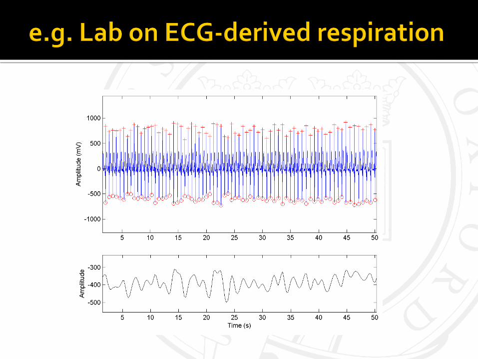
ECG Derived Respiration

Why downsample? Either You need computational efficiency (too much data to process

– not enough RAM / time) Or You want to remove higher frequencies (and then don’t need

to process the higher frequency data)

Sometimes, we need to reduce the sampling rate of a signal. This is downsampling. (The clue is in the name.)

A popular misnomer… downsampling is (wrongly) used synonymously with decimation

Of course, when we downsample to a new sampling rate fs’, we run the risk of lowering our sampling rate below the Nyquist-Shannon limit.

This can lead to aliasing:

Therefore, we should apply a low-pass filter prior to downsampling, to ensure that our signal contains no significant power above fs’ / 2.

Either Your data are missing some important feature (say the QRS

complex is cut off due to low sampling) and you want to restore the feature

You must use a ‘model’ to restore data

Model can be simple or linear, cubic, realistic …

Or Your data are unevenly sampled and your technique requires

an evenly sampled time series (e.g. PSD estimation)

Downsampling is related to decimation – you average out data to reduce noise or compress signal.

Upsampling is a form of interpolation – estimating data in missing points Add zero samples to scale time axis (leads to scaling of frequency axis by

factor 1/N) Must also apply a filter to prevent aliasing!

Both resampling and anti-aliasing are low-pass filters So the more restrictive filter (with the smallest bandwidth) can

be used in place of both the resampling and antialias filters

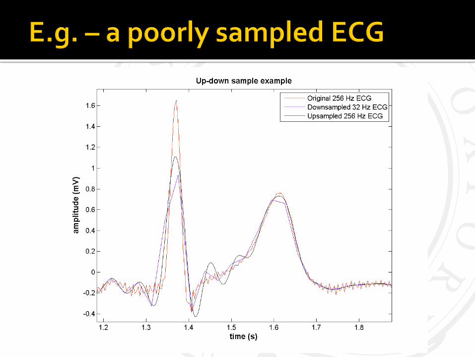
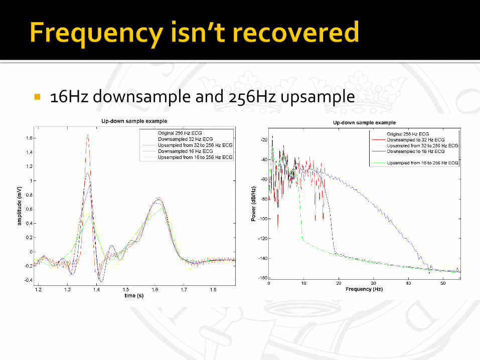
16Hz downsample and 256Hz upsample

Y = RESAMPLE(X,P,Q) resamples the sequence in vector X at

P/Q times the original sample rate using a polyphase implementation:

Upsample P times, downsample Q times Y is P/Q times the length of X (or the ceiling of this if P/Q is not

an integer). P and Q must be positive integers. RESAMPLE applies an anti-aliasing (lowpass) FIR filter to X

during the resampling process, and compensates for the filter's delay.

Interpolation at nodes Sample and hold (Nearest neighbour / piecewise constant interpolation)

▪ Extra high and low frequencies – conservative approach

Linear interpolation ▪ Extra high and low frequencies – more accurate & dangerous?

Polynomial interpolation ▪ Fit curves - – more accurate & dangerous?

Spline interpolation ▪ Better model with more constraints – but unstable -> ringing

Trigonometric interpolation (e.g. by the FFT) See interpft.m – and appendix in slides

Krigging / Interpolation via Gaussian processes

Minmax interpolation

Model-based (e.g. the IPFM for heart rate)

Spectral analysis without interpolation (Lomb-Scargle Periodogram)

See: in

terp

1.m

Invent a regularly spaced grid / define a new set of abscissae

Look at actual points either side of each new abscissa

‘Imagine’ a straight line between the original points

New ordinate value is the value of the line @ intersection with abscissa

Simple, but not a particularly good (smooth) representation of the underlying process though

• Interpolation using high-order polynomials often → ill-behaved results.

• Cubic splines: cubic polynomials approximate curve between each of the N abscissae.

• # cubic polynomials can approximate a curve between two points,

• additional constraints placed on cubic polynomials → result unique.

• The 1st & 2nd derivatives of each cubic polynomial constrained to match @ abscissae.

• all internal cubic polynomials are well defined, with slope and curvature of

approximating polynomials continuous across the abscissae.

Equating the right hand side of the previous two equations gives a quadratic in (x-xn)

This defines the conditions for an optimal cubic polynomial fit to the data.

However, since the first and last polynomials do not have adjoining cubic polynomials additional constraints must be introduced for these two.

The most common approach is to adopt a not-a-knot condition.

This condition forces the third derivative of the first and second cubic polynomials to be identical,

Likewise for the last and second to last cubic polynomials

Finally – you compute derivative of these functions

-- 0.25Hz Sine wave (6Hz sampling) * Downsampled (~1Hz) -∆- Linear interp -+- Cubic spline

Peak at 0.25Hz

Sample and hold introduces lots of high frequency noise

Linear interp less, but more high freq noise than cubic spline

All methods introduce low frequency noise too – why?

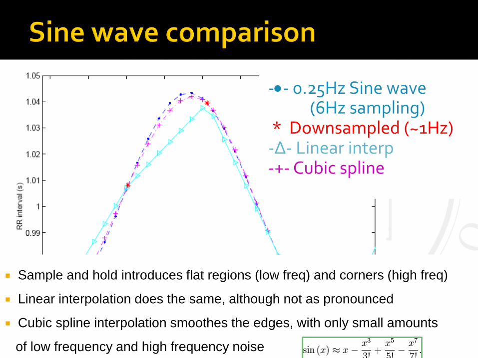
-- 0.25Hz Sine wave (6Hz sampling) * Downsampled (~1Hz) -∆- Linear interp -+- Cubic spline

Sample and hold introduces flat regions (low freq) and corners (high freq)

Linear interpolation does the same, although not as pronounced

Cubic spline interpolation smoothes the edges, with only small amounts

of low frequency and high frequency noise

If there is ‘too much’ missing data, the cubic spline becomes unstable – constraints become too loose

Interpolation/resampling frequency has to be chosen wisely

Not too high to avoid instability

Too low and you will cut corners off the data

Also - look out for noise in the time series – remove

anomalous intervals!

Extrapolation outside of boundaries?

Amplitude Modulation

QRS height (or area)

Due to observational axis changes

Frequency Modulation

RSA

Due to parasympathetic neural modulation

ECG lead (top), HR (middle) and respiration (lower)

How can we measure respiratory rate from this?

Concentrate on deriving it from peaks of ECG

Form time series

Need to resample – why?

Derive features (t,x) – what are they?

Select resample rate – what is a good rate?

Remove noisy beats – why? how?

Select resampling interpolation method – which one?

Estimate respiration rate? How?

Time domain - how?

Frequency domain – how?

Use your peak detector to derive respiration:

From ECG peaks

And from RR intervals if you have the time

Compare …

Friesen et al. (1990) Types of detector

Amplitude threshold

1st derivative

2nd derivative

Digital filters (Energy)

Responses to

Electromyographic noise

Mains

Respiration

Baseline wander

Composite noise

Y = INTERPFT(X,N) returns a vector Y of length N obtained by interpolation in the Fourier transform of X. Assume x(t) is a periodic function of t with period p, sampledat equally spaced points, X(i) = x(T(i)) where

T(i) = (i-1)*p/M, i = 1:M, M = length(X). Then y(t) is another periodic function with the same period and qY(j) = y(T(j)) where T(j) = (j-1)*p/N, j = 1:N, N = length(Y). If N is an integer multiple of M, then Y(1:N/M:N) = X. Example: % Set up a triangle-like signal signal to be interpolated y = [0:.5:2 1.5:-.5:-2 -1.5:.5:0]; % equally spaced factor = 5; % Interpolate by a factor of 5 m = length(y)*factor; x = 1:factor:m; xi = 1:m; yi = interpft(y,m); plot(x,y,'o',xi,yi,'*') legend('Original data','Interpolated data') %Compare to resample: ym = resample(y,factor,1) ;