upscaling of two-phase flow with capillary pressure ... · fine-scale capillary pressure is...
TRANSCRIPT
UPSCALING OF TWO-PHASE FLOW WITH
CAPILLARY PRESSURE HETEROGENEITY EFFECTS
a thesis
submitted to the department of energy resources engineering
of stanford university
in partial fulfillment of the requirements
for the degree of master of science
By
Kasama Itthisawatpan
June 2013

c© Copyright 2013 by Kasama Itthisawatpan
All Rights Reserved
ii
I certify that I have read this thesis and that in my opin-
ion it is fully adequate, in scope and in quality, as a
partial fulfillment of the degree of Master of Science in
Petroleum Engineering.
Prof. Louis J. Durlofsky(Principal Adviser)
iii

iv

Abstract
In this work, we develop a new iterative global upscaling procedure applicable for
two-phase flow with significant capillary pressure heterogeneity effects. These effects
are important to include in simulations of carbon storage operations as they can have
a strong impact on CO2 movement. The upscaling method entails the use of a global
fine-scale two-phase flow simulation for computing the coarse-scale mobility functions.
Two techniques for upscaling capillary pressure are considered. One approach applies
steady-state capillary-limit computations, and the other involves the numerical com-
putation of upscaled capillary pressure along with the upscaled mobilities. For both
approaches, iteration at the coarse-scale level leads to an improvement in the accuracy
of the upscaled model.
The new upscaling procedures are applied to synthetic two-dimensional reservoir
models. Fine-scale capillary pressure is described using the J−function representa-
tion. Different gas injection rates and well locations are considered. The coarse-scale
models generated using the new iterative global upscaling algorithm provide signifi-
cantly more accurate results, relative to reference fine-scale simulations, than do those
based on simpler upscaling procedures. The robustness of the upscaled models is also
assessed, and the models are shown to provide results of reasonable accuracy for cases
involving injection rates or large-scale flow configurations that are different from those
used in the upscaling calculations. This means that the upscaled functions can be
used under a range of flow conditions and are not restricted to only those applied in
the upscaling computations.
v

vi
Acknowledgments
First and foremost, I would like to express my gratitude to my advisor, Professor
Louis Durlofsky, for his support and guidance throughout my study. His insightful
comments and discussions have guided the research toward the right direction, and
his constant encouragement has kept me working through difficult times.
I would also like to thank many researchers and fellow students in the Energy
Resources Engineering Department, including Dr. Huanquan Pan for his help with
GPRS, Dr. Denis Voskov for the discussions on configuring and troubleshooting the
fine-scale simulation with capillary pressure effects, Boxiao Li for the discussion on the
CO2 simulation modeling, Hangyu Li for the discussion on upscaling and for providing
the modified GPRS that was initially used in this work, and David Cameron for the
discussion on the realistic models for field-scale CO2 storage simulation.
I also wish to thank my family for their love and support throughout my study.
Finally, I would like to acknowledge PTT Exploration and Production for their
financial support during both my undergraduate and Master’s careers at Stanford.
vii

viii

Contents
Abstract v
Acknowledgments vii
1 Introduction 1
1.1 Literature Review . . . . . . . . . . . . . . . . . . . . . . . . . . . . . 2
1.1.1 Simulation of CO2 Storage Operations . . . . . . . . . . . . . 2
1.1.2 Significance of Capillary Pressure Heterogeneity . . . . . . . . 3
1.1.3 General Upscaling Methods . . . . . . . . . . . . . . . . . . . 5
1.2 Scope of this Work . . . . . . . . . . . . . . . . . . . . . . . . . . . . 7
1.3 Thesis Outline . . . . . . . . . . . . . . . . . . . . . . . . . . . . . . . 8
2 Upscaling Methods 9
2.1 Upscaling Formulation . . . . . . . . . . . . . . . . . . . . . . . . . . 9
2.1.1 Fine-Scale Governing Equations . . . . . . . . . . . . . . . . . 9
2.1.2 Coarse-Scale Governing Equations . . . . . . . . . . . . . . . . 11
2.1.3 Numerical Calculation of Upscaled Functions . . . . . . . . . . 11
2.2 Upscaling Algorithms . . . . . . . . . . . . . . . . . . . . . . . . . . . 17
2.2.1 Single-Phase Upscaling . . . . . . . . . . . . . . . . . . . . . . 17
2.2.2 Capillary Pressure Calculation . . . . . . . . . . . . . . . . . . 18
2.2.3 Iterative Global Upscaling Method . . . . . . . . . . . . . . . 21
2.2.4 Numerical Calculation of Capillary Pressure . . . . . . . . . . 25
2.2.5 Criteria for Acceptable λ∗j and P ∗c . . . . . . . . . . . . . . . . 27
2.3 Other Methods and Issues . . . . . . . . . . . . . . . . . . . . . . . . 29
ix
2.3.1 Smoothing . . . . . . . . . . . . . . . . . . . . . . . . . . . . . 29
2.3.2 Local k∗ Upscaling with J−Function . . . . . . . . . . . . . . 31
3 Numerical Results 35
3.1 Model Construction . . . . . . . . . . . . . . . . . . . . . . . . . . . . 35
3.1.1 Reservoir Model . . . . . . . . . . . . . . . . . . . . . . . . . . 35
3.2 Upscaling Results . . . . . . . . . . . . . . . . . . . . . . . . . . . . . 39
3.2.1 Flow in x−direction . . . . . . . . . . . . . . . . . . . . . . . 41
3.2.2 Flow in y−direction . . . . . . . . . . . . . . . . . . . . . . . 52
3.3 Robustness to Changes in Boundary Conditions . . . . . . . . . . . . 61
3.3.1 Change in Flow Rate . . . . . . . . . . . . . . . . . . . . . . . 61
3.3.2 Change in Well Locations . . . . . . . . . . . . . . . . . . . . 64
4 Conclusions and Future Work 67
4.1 Conclusions . . . . . . . . . . . . . . . . . . . . . . . . . . . . . . . . 67
4.2 Future Work . . . . . . . . . . . . . . . . . . . . . . . . . . . . . . . . 68
A Additional Numerical Results 69
A.1 Flow in the x−direction . . . . . . . . . . . . . . . . . . . . . . . . . 69
A.1.1 Medium Flow Rate . . . . . . . . . . . . . . . . . . . . . . . . 69
A.1.2 High Flow Rate . . . . . . . . . . . . . . . . . . . . . . . . . . 72
A.2 Flow in the y−direction . . . . . . . . . . . . . . . . . . . . . . . . . 74
A.2.1 Medium Flow Rate . . . . . . . . . . . . . . . . . . . . . . . . 74
A.2.2 High Flow Rate . . . . . . . . . . . . . . . . . . . . . . . . . . 76
Nomenclature 79
Bibliography 82
x
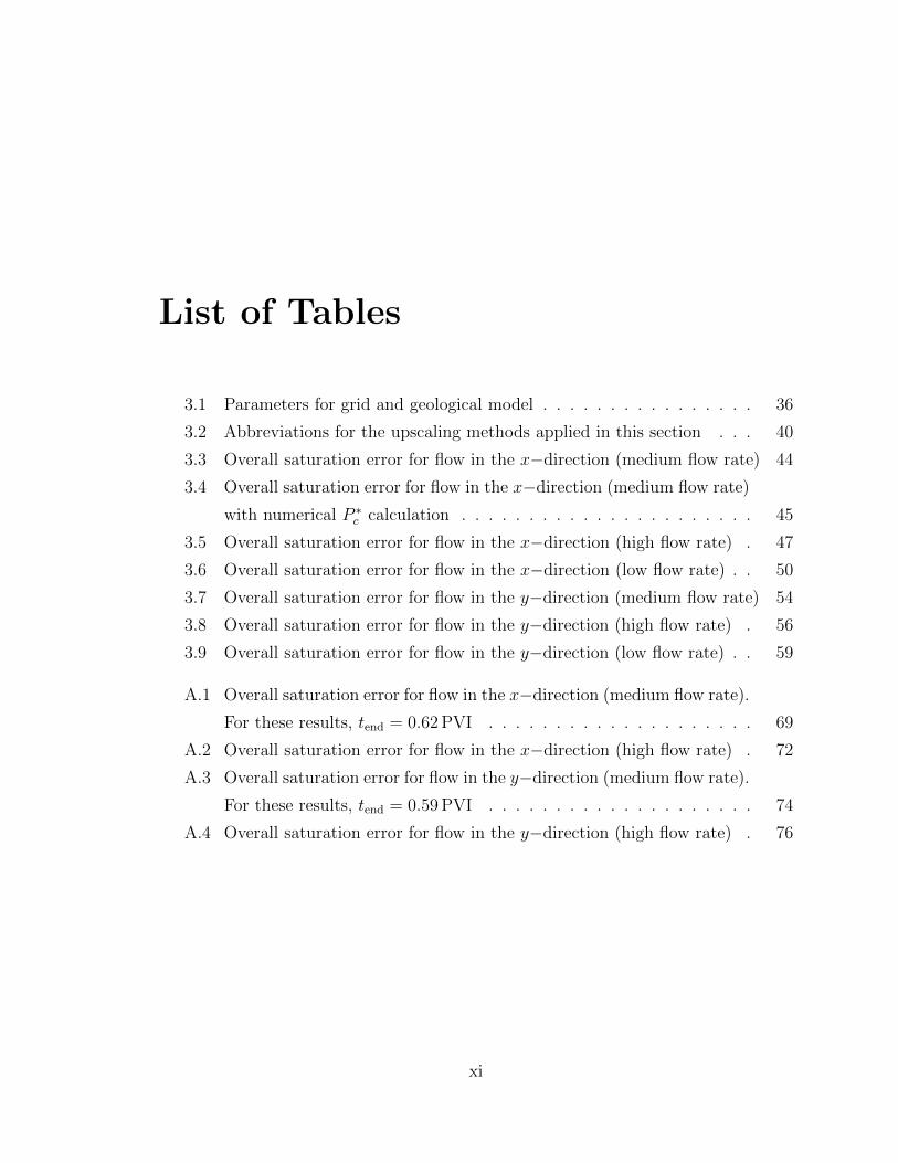
List of Tables
3.1 Parameters for grid and geological model . . . . . . . . . . . . . . . . 36
3.2 Abbreviations for the upscaling methods applied in this section . . . 40
3.3 Overall saturation error for flow in the x−direction (medium flow rate) 44
3.4 Overall saturation error for flow in the x−direction (medium flow rate)
with numerical P ∗c calculation . . . . . . . . . . . . . . . . . . . . . . 45
3.5 Overall saturation error for flow in the x−direction (high flow rate) . 47
3.6 Overall saturation error for flow in the x−direction (low flow rate) . . 50
3.7 Overall saturation error for flow in the y−direction (medium flow rate) 54
3.8 Overall saturation error for flow in the y−direction (high flow rate) . 56
3.9 Overall saturation error for flow in the y−direction (low flow rate) . . 59
A.1 Overall saturation error for flow in the x−direction (medium flow rate).
For these results, tend = 0.62 PVI . . . . . . . . . . . . . . . . . . . . 69
A.2 Overall saturation error for flow in the x−direction (high flow rate) . 72
A.3 Overall saturation error for flow in the y−direction (medium flow rate).
For these results, tend = 0.59 PVI . . . . . . . . . . . . . . . . . . . . 74
A.4 Overall saturation error for flow in the y−direction (high flow rate) . 76
xi
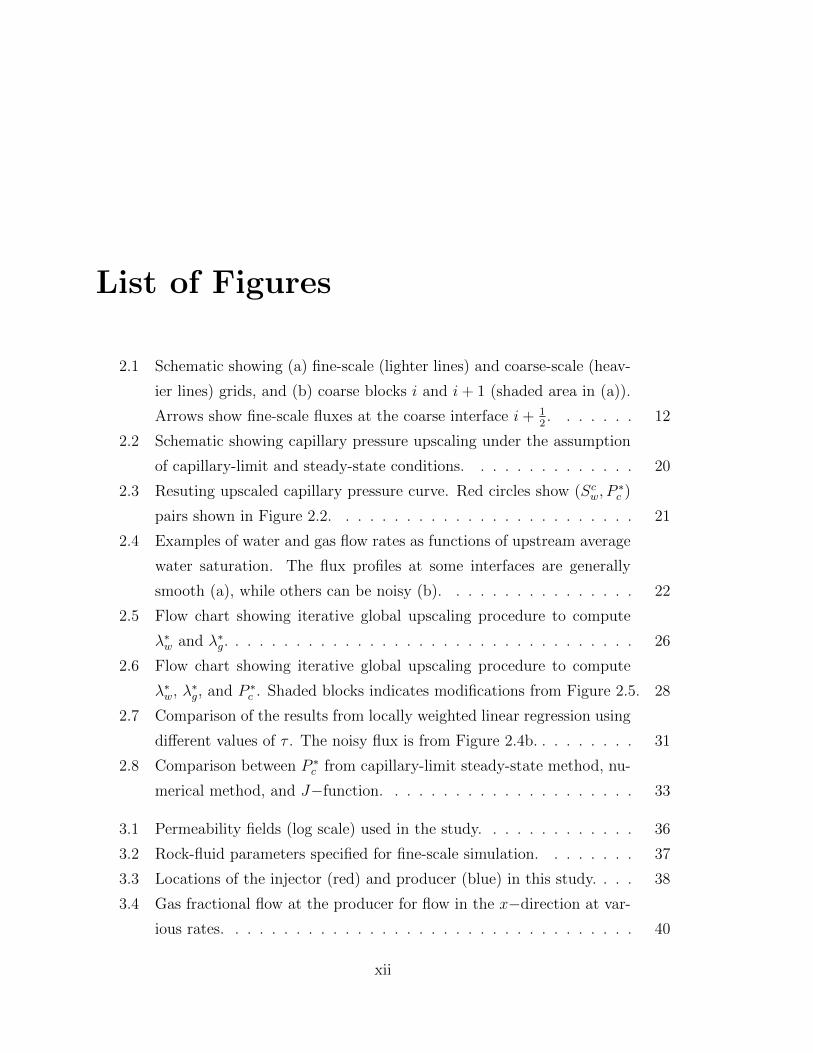
List of Figures
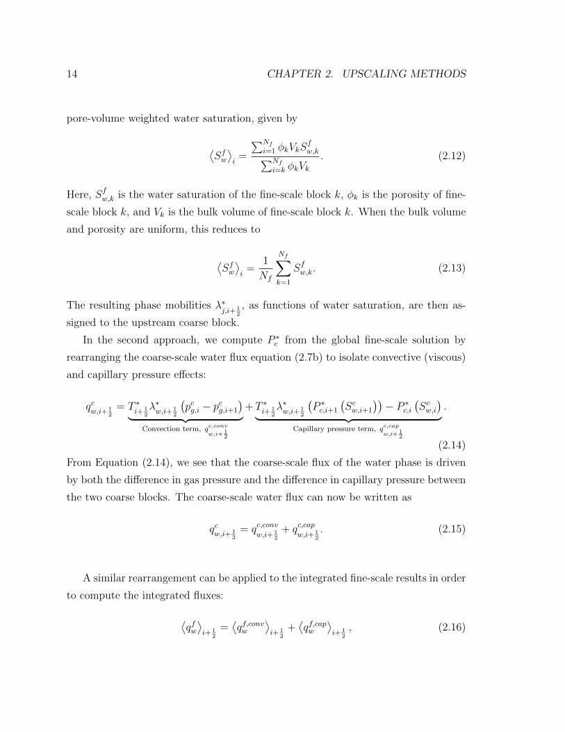
2.1 Schematic showing (a) fine-scale (lighter lines) and coarse-scale (heav-
ier lines) grids, and (b) coarse blocks i and i+ 1 (shaded area in (a)).
Arrows show fine-scale fluxes at the coarse interface i+ 12. . . . . . . 12
2.2 Schematic showing capillary pressure upscaling under the assumption
of capillary-limit and steady-state conditions. . . . . . . . . . . . . . 20
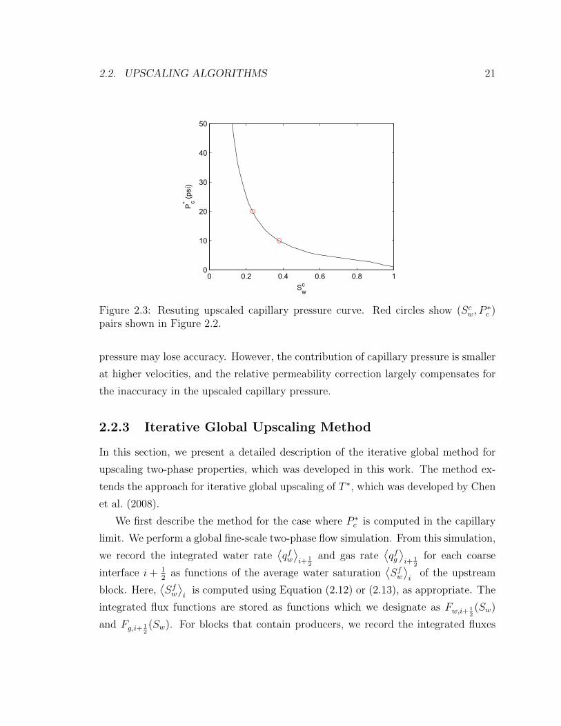
2.3 Resuting upscaled capillary pressure curve. Red circles show (Scw, P∗c )
pairs shown in Figure 2.2. . . . . . . . . . . . . . . . . . . . . . . . . 21
2.4 Examples of water and gas flow rates as functions of upstream average
water saturation. The flux profiles at some interfaces are generally
smooth (a), while others can be noisy (b). . . . . . . . . . . . . . . . 22
2.5 Flow chart showing iterative global upscaling procedure to compute
λ∗w and λ∗g. . . . . . . . . . . . . . . . . . . . . . . . . . . . . . . . . . 26
2.6 Flow chart showing iterative global upscaling procedure to compute
λ∗w, λ∗g, and P ∗c . Shaded blocks indicates modifications from Figure 2.5. 28
2.7 Comparison of the results from locally weighted linear regression using
different values of τ . The noisy flux is from Figure 2.4b. . . . . . . . . 31
2.8 Comparison between P ∗c from capillary-limit steady-state method, nu-
merical method, and J−function. . . . . . . . . . . . . . . . . . . . . 33
3.1 Permeability fields (log scale) used in the study. . . . . . . . . . . . . 36
3.2 Rock-fluid parameters specified for fine-scale simulation. . . . . . . . 37
3.3 Locations of the injector (red) and producer (blue) in this study. . . . 38
3.4 Gas fractional flow at the producer for flow in the x−direction at var-
ious rates. . . . . . . . . . . . . . . . . . . . . . . . . . . . . . . . . . 40
xii
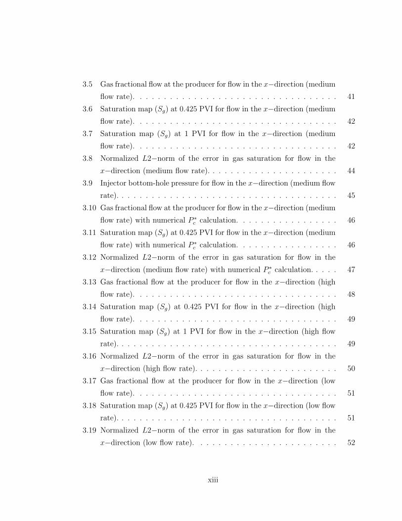
3.5 Gas fractional flow at the producer for flow in the x−direction (medium
flow rate). . . . . . . . . . . . . . . . . . . . . . . . . . . . . . . . . . 41
3.6 Saturation map (Sg) at 0.425 PVI for flow in the x−direction (medium
flow rate). . . . . . . . . . . . . . . . . . . . . . . . . . . . . . . . . . 42
3.7 Saturation map (Sg) at 1 PVI for flow in the x−direction (medium
flow rate). . . . . . . . . . . . . . . . . . . . . . . . . . . . . . . . . . 42
3.8 Normalized L2−norm of the error in gas saturation for flow in the
x−direction (medium flow rate). . . . . . . . . . . . . . . . . . . . . . 44
3.9 Injector bottom-hole pressure for flow in the x−direction (medium flow
rate). . . . . . . . . . . . . . . . . . . . . . . . . . . . . . . . . . . . . 45
3.10 Gas fractional flow at the producer for flow in the x−direction (medium
flow rate) with numerical P ∗c calculation. . . . . . . . . . . . . . . . . 46
3.11 Saturation map (Sg) at 0.425 PVI for flow in the x−direction (medium
flow rate) with numerical P ∗c calculation. . . . . . . . . . . . . . . . . 46
3.12 Normalized L2−norm of the error in gas saturation for flow in the
x−direction (medium flow rate) with numerical P ∗c calculation. . . . . 47
3.13 Gas fractional flow at the producer for flow in the x−direction (high
flow rate). . . . . . . . . . . . . . . . . . . . . . . . . . . . . . . . . . 48
3.14 Saturation map (Sg) at 0.425 PVI for flow in the x−direction (high
flow rate). . . . . . . . . . . . . . . . . . . . . . . . . . . . . . . . . . 49
3.15 Saturation map (Sg) at 1 PVI for flow in the x−direction (high flow
rate). . . . . . . . . . . . . . . . . . . . . . . . . . . . . . . . . . . . . 49
3.16 Normalized L2−norm of the error in gas saturation for flow in the
x−direction (high flow rate). . . . . . . . . . . . . . . . . . . . . . . . 50
3.17 Gas fractional flow at the producer for flow in the x−direction (low
flow rate). . . . . . . . . . . . . . . . . . . . . . . . . . . . . . . . . . 51
3.18 Saturation map (Sg) at 0.425 PVI for flow in the x−direction (low flow
rate). . . . . . . . . . . . . . . . . . . . . . . . . . . . . . . . . . . . . 51
3.19 Normalized L2−norm of the error in gas saturation for flow in the
x−direction (low flow rate). . . . . . . . . . . . . . . . . . . . . . . . 52
xiii

3.20 Gas fractional flow at the producer for flow in the y−direction (medium
flow rate). . . . . . . . . . . . . . . . . . . . . . . . . . . . . . . . . . 53
3.21 Saturation map (Sg) at 0.425 PVI for flow in the y−direction (medium
flow rate). . . . . . . . . . . . . . . . . . . . . . . . . . . . . . . . . . 53
3.22 Normalized L2−norm of the error in gas saturation for flow in the
y−direction (medium flow rate). . . . . . . . . . . . . . . . . . . . . . 54
3.23 Average gas saturation at the top layer for flow in the y−direction
(medium flow rate). . . . . . . . . . . . . . . . . . . . . . . . . . . . . 55
3.24 Injector bottom-hole pressure for flow in the y−direction (medium flow
rate). . . . . . . . . . . . . . . . . . . . . . . . . . . . . . . . . . . . . 56
3.25 Gas fractional flow at the producer for flow in the y−direction (high
flow rate). . . . . . . . . . . . . . . . . . . . . . . . . . . . . . . . . . 57
3.26 Saturation map (Sg) at 0.425 PVI for flow in the y−direction (high
flow rate). . . . . . . . . . . . . . . . . . . . . . . . . . . . . . . . . . 57
3.27 Normalized L2−norm of the error in gas saturation for flow in the
y−direction (high flow rate). . . . . . . . . . . . . . . . . . . . . . . . 58
3.28 Average gas saturation at the top layer for flow in the y−direction
(high flow rate). . . . . . . . . . . . . . . . . . . . . . . . . . . . . . . 58
3.29 Gas fractional flow at the producer for flow in the y−direction (low
flow rate). . . . . . . . . . . . . . . . . . . . . . . . . . . . . . . . . . 59
3.30 Saturation map (Sg) at 0.425 PVI for flow in the y−direction (low flow
rate). . . . . . . . . . . . . . . . . . . . . . . . . . . . . . . . . . . . . 60
3.31 Normalized L2−norm of the error in gas saturation for flow in the
y−direction (low flow rate). . . . . . . . . . . . . . . . . . . . . . . . 60
3.32 Average gas saturation at the top layer for flow in the y−direction (low
flow rate). . . . . . . . . . . . . . . . . . . . . . . . . . . . . . . . . . 61
3.33 Overall saturation error for G1P/iG2P30 and G1P/iG2P60, with G1P/iG2P
and G1P/Pc shown for reference (flow in the x−direction). . . . . . . 62
3.34 Overall saturation error for G1P/iG2P30 and G1P/iG2P60, with G1P/iG2P
and G1P/Pc shown for reference (flow in the y−direction). . . . . . . 63
xiv

3.35 Gas fractional flow at the producer for flow in the x−direction at low
rate (10 bbl/day) using various models. . . . . . . . . . . . . . . . . . 63
3.36 Gas fractional flow at the producer for flow in the x−direction at high
rate (100 bbl/day) using various models. . . . . . . . . . . . . . . . . 64
3.37 Gas fractional flow at the producer for corner-to-corner flow (high flow
rate). . . . . . . . . . . . . . . . . . . . . . . . . . . . . . . . . . . . . 65
3.38 Saturation map at 0.425 PVI for the corner-to-corner flow (high flow
rate). . . . . . . . . . . . . . . . . . . . . . . . . . . . . . . . . . . . . 66
A.1 Gas fractional flow at the producer for flow in the x−direction (medium
flow rate). . . . . . . . . . . . . . . . . . . . . . . . . . . . . . . . . . 70
A.2 Saturation map (Sg) at 0.425 PVI for flow in the x−direction (medium
flow rate). . . . . . . . . . . . . . . . . . . . . . . . . . . . . . . . . . 70
A.3 Normalized L2−norm of the error in gas saturation for flow in the
x−direction (medium flow rate). . . . . . . . . . . . . . . . . . . . . . 71
A.4 Gas fractional flow at the producer for flow in the x−direction (high
flow rate). . . . . . . . . . . . . . . . . . . . . . . . . . . . . . . . . . 72
A.5 Saturation map (Sg) at 0.425 PVI for flow in the x−direction (high
flow rate). . . . . . . . . . . . . . . . . . . . . . . . . . . . . . . . . . 73
A.6 Normalized L2−norm of the error in gas saturation for flow in the
x−direction (high flow rate). . . . . . . . . . . . . . . . . . . . . . . . 73
A.7 Gas fractional flow at the producer for flow in the y−direction (medium
flow rate). . . . . . . . . . . . . . . . . . . . . . . . . . . . . . . . . . 74
A.8 Saturation map (Sg) at 0.425 PVI for flow in the y−direction (medium
flow rate). . . . . . . . . . . . . . . . . . . . . . . . . . . . . . . . . . 75
A.9 Normalized L2−norm of the error in gas saturation for flow in the
y−direction (medium flow rate). . . . . . . . . . . . . . . . . . . . . . 75
A.10 Gas fractional flow at the producer for flow in the y−direction (high
flow rate). . . . . . . . . . . . . . . . . . . . . . . . . . . . . . . . . . 76
A.11 Saturation map (Sg) at 0.425 PVI for flow in the y−direction (high
flow rate). . . . . . . . . . . . . . . . . . . . . . . . . . . . . . . . . . 77
xv
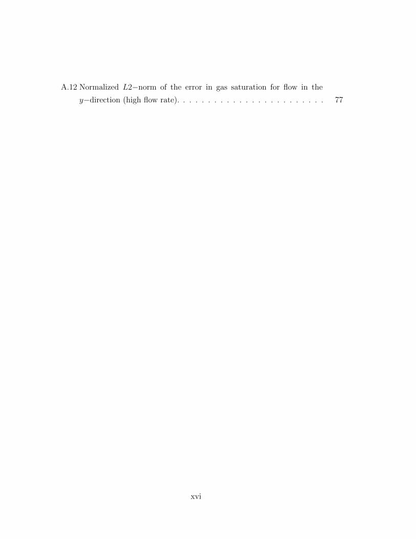
A.12 Normalized L2−norm of the error in gas saturation for flow in the
y−direction (high flow rate). . . . . . . . . . . . . . . . . . . . . . . . 77
xvi
Chapter 1
Introduction
The sequestration of carbon dioxide in deep geological formations is being considered
as a means to mitigate the impact of fossil fuel combustion. The idea is to capture
CO2 at the power plant and to inject it into various types of subsurface formations
such as depleted oil and gas reservoirs and deep saline aquifers. The injected carbon
dioxide is “stored” in the subsurface through some combination of structural trapping,
residual trapping, dissolution trapping, and mineral trapping.
In order to minimize the environmental risk, the movement and the distribution
of the injected CO2 must be accurately modeled. Because the flow of supercritical
CO2 in subsurface formations entails very similar physical phenomena as the flow of
fluids in oil and gas reservoirs, petroleum reservoir simulators can be used to model
the flow of the injected CO2. As is the case for the flow of oil and gas in the sub-
surface, the flow of CO2 involves effects at various scales. Fine-scale geostatistical
models may include blocks of O(1− 10 m), while full-field simulations are often per-
formed with blocks of O(10−100 m). In many cases, especially in models with strong
heterogeneity, fine-scale property variation can significantly influence simulation re-
sults. In order to achieve accurate coarse-scale simulations, this heterogeneity must
be properly accounted for in the coarse-scale model. This scale translation can be
accomplished using the methods of upscaling.
Although many of the general issues that arise in the upscaling of carbon storage
1
2 CHAPTER 1. INTRODUCTION
models are similar to those in oil and gas simulation, there are some important dif-
ferences. Oil and gas simulations usually involve sufficiently high flow rates such that
viscous and gravitational forces dominate in full-field simulations. Carbon storage,
by contrast, can entail much lower rates, so capillary effects must also be treated in
field-scale simulations. This introduces challenges in the upscaling of the equations
governing the carbon storage processes.
Our goal in this work is to devise and test new upscaling methods that enable
accurate large-scale simulation of two-phase flow problems with significant capillary
pressure effects. This will require us to incorporate new treatments into two-phase
upscaling procedures.
1.1 Literature Review
1.1.1 Simulation of CO2 Storage Operations
Simulation of field-scale carbon storage in deep saline aquifers has been addressed by
various authors in recent years. The simulations typically include about 30 years of
CO2 injection, followed by an equilibration period, which can last for several hun-
dred years, during which the injected gas equilibrates in the aquifer. Studies have
varied from conceptual assessments of key mechanisms to actual field-scale simula-
tions. As the primary goal is usually to predict the distribution of the injected CO2,
the conceptual studies have investigated the factors that affect the final CO2 plume
location. For example, Mo and Akervoll (2005) used a black-oil model to characterize
the impact of permeability anisotropy, relative permeability, and capillary pressure
characteristics on the gas stored by structural and residual trapping. Ide et al. (2007)
examined the interaction between viscous, capillary, and gravitational forces more
systematically, by comparing different scenarios in terms of their gravity numbers
and capillary numbers. They concluded that scenarios with relatively low gravitata-
tional forces compared to viscous forces resulted in more residually-trapped CO2.
Increasing the magnitude of capillary forces compared to the other forces contributed
to more, and faster, CO2 trapping. Dissolution trapping was not considered in detail
1.1. LITERATURE REVIEW 3
by Ide et al. (2007).
Some authors also investigated dissolution trapping in addition to residual trap-
ping. Kumar et al. (2004) and Ghanbari et al. (2006) applied compositional models
to study the impact of various factors on dissolution trapping. Recently, field-scale
case studies (e.g., Doughty, 2010; Han et al., 2010; Chasset et al., 2011) incorporated
the actual aquifer geometry and petrophysical properties into the simulation models.
The results obtained from the field-scale studies generally agreed with the concep-
tual studies in terms of the impact of reservoir properties on residual and dissolution
trapping. They observed, however, that reservoir heterogeneity also has a significant
impact on the movement of CO2 and the final plume location. The results from the
case studies also indicated the need for accurate models for the spatial distribution
of petrophysical properties.
1.1.2 Significance of Capillary Pressure Heterogeneity
Recent studies have also highlighted the importance of capillary pressure heterogene-
ity on CO2 plume migration. Capillary pressure heterogeneity is often ignored in sub-
surface flow modeling. More specifically, it is common to neglect capillary pressure en-
tirely or to assign a single capillary pressure curve to all simulation blocks. Saadatpoor
et al. (2010) incorporated capillary pressure heterogeneity based on the J−function
representation (Leverett, 1940) in a highly heterogeneous fine-scale model. They
compared the ultimate distribution of the injected CO2 with a model that had the
same permeability field but homogeneous capillary pressure. Their conclusion was
that capillary pressure heterogeneity strongly impacted the flow of the CO2. Capil-
lary pressure heterogeneity results in a strong barrier to the flow of the nonwetting
phase, so the injected gas can be immobilized even though its saturation is signif-
icantly higher than the residual saturation. The authors referred to this trapping
phenomenon as the “local capillary trapping” mechanism.
The effects of capillary heterogeneity have also been found to be significant at the
core scale. Krevor et al. (2011) and Li et al. (2012) applied theoretical, experimen-
tal, and numerical simulation approaches to analyze the impact of capillary pressure

4 CHAPTER 1. INTRODUCTION
heterogeneity on the distribution of fluids in the core. They injected CO2 at rates
that are comparable to those in CO2 storage operations and showed that the final
fluid distribution is highly nonuniform. Experiments were performed by having a
drainage process (CO2 injection) followed by an imbibition process (water flooding).
The overall CO2 saturation after the water flooding was much higher than would be
expected if capillary pressure heterogeneity were not included (Krevor et al., 2011).
The observation that capillary pressure heterogeneity affects flow at both the core
scale and the geostatistical scale necessitates the accurate fine-scale modeling of cap-
illary pressure heterogeneity. However, the use of very fine grid blocks in a full-field
simulation is not practical and would be computationally expensive. In order to cap-
ture fine-scale heterogeneity effects in the coarse-scale domain, some studies have in-
troduced procedures to upscale capillary pressure. For example, Mouche et al. (2010)
used the analytical solution for flow in a vertical, one-dimensional periodic layered
porous medium under the capillary-limit condition to compute the upscaled capil-
lary pressure. Behzadi and Alvarado (2012) modified the capillary-limit steady-state
calculation presented by Pickup and Sorbie (1996) to account for the flow direction
and the subgrid spatial distribution of the capillary pressure. These methods were
shown to provide accurate coarse-scale flow results, though they are applicable only
to very specific flow conditions which may not be encountered in realistic field-scale
simulations.
Saadatpoor et al. (2011) presented an alternative approach to upscale the capillary
pressure from the geostatistical scale to the field scale. They computed an “effective”
permeability for each coarse grid block as the geometric mean of the underlying
fine-scale permeabilities, and then applied the J−function based on this effective
permeability to provide an upscaled capillary pressure. Saadatpoor et al. (2011)
concluded that this upscaled model did not preserve the local capillary trapping
observed in the fine-scale model. The calculation of the upscaled capillary pressure
in Saadatpoor et al. (2011) does not assume specific flow conditions, so the approach
can be applied to generic flow conditions. However, it represents a highly simplified
approach for capillary pressure upscaling. In order to achieve more accurate coarse-
scale results, a more sophisticated flow-based upscaling method, which also treats
1.1. LITERATURE REVIEW 5
relative permeability, will be needed. We now provide a brief discussion of upscaling
techniques that may be relevant for this problem.
1.1.3 General Upscaling Methods
Upscaling involves the calculation of coarse-scale properties and flow functions that
can accurately capture underlying fine-scale effects. When used in coarse-scale simu-
lations, properly computed upscaled functions can provide flow predictions in general
agreement with fine-scale results. Upscaling methods can be categorized in different
ways. For example, single-phase upscaling methods provide equivalent flow properties
such as porosity, absolute permeability, and transmissibility. Two-phase (or multi-
phase) upscaling provides transport functions such as capillary pressure and relative
permeability.
Another way to view upscaling procedures is based on the domain on which the
effective properties are computed. Methods can be described as local, extended lo-
cal, and global upscaling procedures. For example, local upscaling entails fine-scale
simulation over the domain corresponding to the target coarse block with assumed
pressure and saturation boundary conditions. Extended-local methods also require
assumptions on the boundary conditions, but the local fine-scale simulations include
additional (neighboring) cells. Global upscaling, by contrast, uses the information
from global fine-scale simulation to compute effective properties. In general, the
global (or local-global, where global information is provided by coarse-scale simula-
tions) calculation of transmissibility has been shown to provide the most accurate
single-phase upscaling (Chen et al., 2003; Chen et al., 2010). Since this work entails
the calculation of upscaled two-phase properties, our focus will be on multiphase up-
scaling procedures. Refer to Durlofsky (2005) for further discussion of single-phase
upscaling and related issues.
Ekrann and Dale (1992) classified multiphase upscaling into “dynamic” and “effec-
tive” upscaling procedures. Effective upscaling entails calculations based on local so-
lutions for particular limiting cases. For example, Pickup and Sorbie (1996) developed

6 CHAPTER 1. INTRODUCTION
steady-state methods to compute effective capillary pressure and relative permeabil-
ity which are valid for either the capillary or the viscous limit. Virnovsky et al. (2004)
further developed the steady-state method. They showed that, as the imposed pres-
sure drop was increased or decreased, the resulting upscaled functions approached the
viscous limit or the capillary limit results, respectively. These steady-state approaches
are generally computationally efficient, though their accuracy strongly depends on the
applicability of the assumed conditions.
Dynamic upscaling, by contrast, involves time-dependent fine-scale simulations
over specified (e.g., local or global) domains. Upscaled capillary pressure and/or
relative permeability are computed based on a coarse-scale Darcy’s law such that
the flux of each phase on the coarse scale matches the integrated flux from the fine-
scale results. As is the case in single-phase upscaling, assumptions on local boundary
conditions often influence the accuracy of upscaled properties computed using local
or extended-local methods.
Darman et al. (2002) evaluated the dynamic upscaling procedures proposed by
Kyte and Berry (1975), Stone (1991), Hewett and Archer (1997), and Darman and
Pickup (1999). They performed global upscaling for several cases and found that the
Hewett and Archer (1997) method and the transmissibility-weighted method (Dar-
man and Pickup, 1999) provided the most accurate coarse models both with and
without significant gravitational effects. However, this study only involved purely
layered permeability distributions; systems with random fine-scale permeability fields
were not considered. Local property variation is, however, of significant interest for
our problem. The effects of capillary pressure were also neglected in the examples
presented by Darman et al. (2002).
More recent developments in multiphase upscaling have considered random fine-
scale permeability fields. Wallstrom et al. (2002) developed so-called effective flux
boundary conditions (EFBCs) for local upscaling in the viscous limit. EFBCs pro-
vide pressure boundary conditions based on the local fine-scale permeability field.
A detailed investigation by Chen (2005) showed that the use of EFBCs resulted in
substantially more accurate coarse-scale models than the use of standard boundary
conditions (constant pressure at the inlet and outlet) in many cases. Chen and Li
1.2. SCOPE OF THIS WORK 7
(2009) developed an adaptive local-global method to compute upscaled relative per-
meability. The coarse-scale results based on the two-phase local-global upscaling were
shown to match the fine-scale results for various variogram-based models. The ap-
proaches described above represent reasonable approaches for two-phase upscaling,
though they are based on viscous-dominated flow, with capillary pressure neglected.
Upscaling of two-phase flow with capillary pressure heterogeneity was considered
by Lohne et al. (2006). They applied the capillary-limit steady-state method to
upscale capillary pressure. Other methods, including both steady-state and dynamic
approaches, were applied to upscale relative permeability. Capillary-limit effective
capillary pressure, together with appropriate relative permeability upscaling based
on the capillary number, was shown to provide accurate coarse-scale models. The
reservoir models presented in Lohne et al. (2006) somewhat resemble those considered
in this work, in that both realistic permeability heterogeneity and capillary pressure
heterogeneity were included. However, the capillary pressure heterogeneity in Lohne
et al. (2006) was modeled using a conceptual, checkerboard pattern at the fine scale,
and by the use of rock types at the geostatistical scale. Thus, the capillary pressure
did not depend directly on the local permeability distribution. In this work, we
consider a more general model, with capillary pressure heterogeneity represented by
the J−function. In addition, the upscaling procedure developed here uses global flow
information, in contrast to the approach applied by Lohne et al. (2006).
1.2 Scope of this Work
In this work, we focus on the two-phase upscaling of flow with significant capillary
pressure heterogeneity effects. We assess approaches for the calculation of upscaled
capillary pressure functions. The upscaled relative permeability is computed from
global fine-scale solutions. We focus on scenarios that are relevant for CO2 storage
simulations, though some of the physics that is important in CO2 storage, such as
gravitational effects, dissolution, and relative permeability hysteresis, is not included
in our simulations. The resulting coarse-scale models are assessed by comparing the
coarse-scale results, including the fractional flow of gas at the production well and
8 CHAPTER 1. INTRODUCTION
the phase saturation distributions, with fine-scale results.
Computing the upscaled functions from global fine-scale flows is challenging for
highly heterogeneous systems with low flow rates, as unphysical upscaled functions
can result unless appropriate treatments are applied. In this work, we develop an
iterative scheme to improve coarse-scale results. Because the methods developed in
this work involve global fine-scale, two-phase flow simulations, which are essentially
what we wish to avoid, it is important that the resulting coarse model is applicable
for other flow scenarios. We therefore assess the robustness of the resulting upscaled
functions with respect to changes in boundary conditions. For this assessment, we run
a global fine-scale simulation for a representative case, and then apply the upscaled
functions computed for this model to cases that involve different flow conditions.
Coarse-scale solutions for changing injection rates and well locations will be presented
and assessed.
1.3 Thesis Outline
This thesis is organized as follows:
• Chapter 2 presents the formulation for the upscaling problem. The fine-scale
and coarse-scale governing equations are discussed, and the computation of the
upscaled functions is explained. We discuss several approaches for upscaling
capillary pressure, as well as the calculation of upscaled relative permeability
using an iterative global upscaling scheme.
• Chapter 3 presents numerical examples that quantify the performance of dif-
ferent upscaling methods. The methods are applied for different well locations
and CO2 injection rates. Then, we assess the robustness of the upscaled model
under changes in injection rates and well locations.
• Chapter 4 includes a summary and conclusions for this work. Suggestions for
future research are also provided.
• Appendix A includes upscaling results for another geological model.
Chapter 2
Upscaling Methods
In this chapter, we present the governing equations for the flow of gas and water in
porous media at both the fine-scale and the coarse-scale levels. We briefly summarize
the existing upscaling methods that are applied in this study. Then, we describe in
detail our treatment for capillary pressure and the iterative two-phase global upscaling
approach. This is a new method that was developed in this work. In describing the
iterative two-phase global upscaling procedure, we also discuss several key aspects of
the implementation.
2.1 Upscaling Formulation
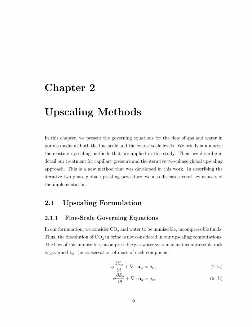
2.1.1 Fine-Scale Governing Equations
In our formulation, we consider CO2 and water to be immiscible, incompressible fluids.
Thus, the dissolution of CO2 in brine is not considered in our upscaling computations.
The flow of this immiscible, incompressible gas-water system in an incompressible rock
is governed by the conservation of mass of each component
φ∂Sw∂t
+∇ · uw = qw, (2.1a)
φ∂Sg∂t
+∇ · ug = qg, (2.1b)
9
10 CHAPTER 2. UPSCALING METHODS
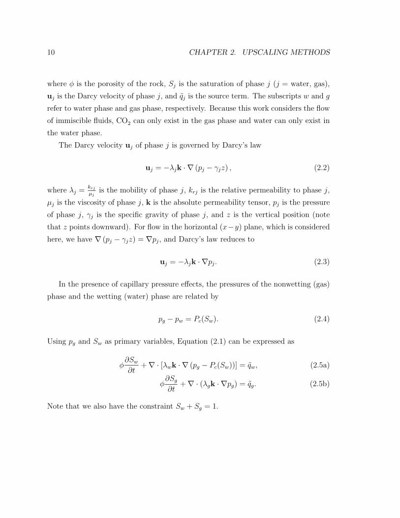
where φ is the porosity of the rock, Sj is the saturation of phase j (j = water, gas),
uj is the Darcy velocity of phase j, and qj is the source term. The subscripts w and g
refer to water phase and gas phase, respectively. Because this work considers the flow
of immiscible fluids, CO2 can only exist in the gas phase and water can only exist in
the water phase.
The Darcy velocity uj of phase j is governed by Darcy’s law
uj = −λjk · ∇ (pj − γjz) , (2.2)
where λj =krjµj
is the mobility of phase j, krj is the relative permeability to phase j,
µj is the viscosity of phase j, k is the absolute permeability tensor, pj is the pressure
of phase j, γj is the specific gravity of phase j, and z is the vertical position (note
that z points downward). For flow in the horizontal (x−y) plane, which is considered
here, we have ∇ (pj − γjz) = ∇pj, and Darcy’s law reduces to
uj = −λjk · ∇pj. (2.3)
In the presence of capillary pressure effects, the pressures of the nonwetting (gas)
phase and the wetting (water) phase are related by
pg − pw = Pc(Sw). (2.4)
Using pg and Sw as primary variables, Equation (2.1) can be expressed as
φ∂Sw∂t
+∇ · [λwk · ∇ (pg − Pc(Sw))] = qw, (2.5a)
φ∂Sg∂t
+∇ · (λgk · ∇pg) = qg. (2.5b)
Note that we also have the constraint Sw + Sg = 1.
2.1. UPSCALING FORMULATION 11
2.1.2 Coarse-Scale Governing Equations
The coarse-scale governing equations can be constructed by averaging the fine-scale
equations over the region corresponding to a single coarse block. Refer to Chen
(2005) for detailed formulations and discussion of the different forms of the coarse-
scale equations. In this work, we restrict the coarse-scale equations to have the same
general form as the fine-scale equations, but with upscaled properties and functions
replacing their fine-scale analogs. The conservation equations for the coarse-scale
system can thus be written as
φ∗∂Scw
∂t+∇ ·
[λ∗wk∗ · ∇
(pcg − P ∗
c (Scw))]
= qcw, (2.6a)
φ∗∂Scg
∂t+∇ ·
(λ∗gk
∗ · ∇pcg)
= qcg, (2.6b)
where the superscript c represents a coarse-scale variable, and the superscript ∗ indi-
cates a precomputed coarse-scale property or function.
2.1.3 Numerical Calculation of Upscaled Functions
If the coarse-scale equations (2.6) are discretized using a two-point flux approximation
and the usual upstream weighting, the flux of each phase j across a coarse interface
i+ 12
between two coarse blocks i and i+ 1, designated qcj,i+ 1
2
, can be written as
qcg,i+ 1
2= T ∗
i+ 12λ∗g,i+ 1
2
(pcg,i − pcg,i+1
), (2.7a)
for the gas phase, and
qcw,i+ 1
2= T ∗
i+ 12λ∗w,i+ 1
2
[(pcg,i − P ∗
c,i
(Scw,i
))−(pcg,i+1 − P ∗
c,i+1
(Scw,i+1
))], (2.7b)
for the water phase. Here T ∗i+ 1
2
is the upscaled transmissibility, which will be discussed
below. For the blocks containing wells, the flux of phase j from block i to the wellbore,
12 CHAPTER 2. UPSCALING METHODS
designated as qcwell,j,i, can be written as
qcwell,j,i = WI∗i λ∗j,i
(pcg,i − pcwell,i
), (2.8)
where WI∗i is the upscaled well index and pcwell,i is the well pressure in block i.
The upscaled single-phase parameters, transmissibility T ∗i+ 1
2
and well index WI∗i ,
can be computed from a single-phase upscaling algorithm, which will be described
in the next section. Once the single-phase parameters have been computed, the goal
of two-phase upscaling is to provide coarse-scale fluxes that match the sum of the
corresponding fine-scale fluxes:
qcg,i+ 1
2=⟨qfg⟩i+ 1
2
, qcw,i+ 1
2=⟨qfw⟩i+ 1
2
, (2.9)
where the superscript f indicates that the quantity is from fine-scale simulation and
〈·〉i+ 12
denotes the integrated flux over the fine-scale interfaces that correspond to the
coarse interface i+ 12. This is illustrated in Figure 2.1. The equations are analogous
for blocks that contain wells.
(a)
coarse block i! coarse block i +1!
(b)
Figure 2.1: Schematic showing (a) fine-scale (lighter lines) and coarse-scale (heavierlines) grids, and (b) coarse blocks i and i + 1 (shaded area in (a)). Arrows showfine-scale fluxes at the coarse interface i+ 1
2.
2.1. UPSCALING FORMULATION 13
Expressions (2.9) constitute two equations for the upscaling computations. How-
ever, with nonzero capillary pressure, three upscaled functions, λ∗w, λ∗g, and P ∗c , must
be determined for each coarse block. In order to solve this underdetermined system,
we consider two different approaches: (1) we first compute P ∗c (Scw) analytically, under
a steady-state assumption, followed by the calculation of λ∗j(Scw) via global upscal-
ing, and (2) we identify the capillary and convective flux contributions to qcw,i+ 1
2
and
compute the upscaled functions accordingly. We now describe these two approaches
in detail.
In the first approach, the upscaled capillary pressure function for each coarse
block is precomputed using an analytical approach. No flow simulation is required
because we assume steady-state conditions. The detailed calculation will be discussed
in the next section. With these precomputed capillary pressure functions, only two
upscaled functions remain to be computed, so the problem is now well-defined. The
upscaled mobility for each phase can then be computed from the fine-scale solution by
rearranging Equations (2.7a) and (2.7b) and approximating the coarse-scale pressure
and saturation as averages of the fine-scale results
λ∗g,i+ 1
2=
⟨qfg⟩i+ 1
2
T ∗i+ 1
2
(⟨pfg⟩i−⟨pfg⟩i+1
) , (2.10a)
λ∗w,i+ 1
2=
⟨qfw⟩i+ 1
2
T ∗i+ 1
2
[⟨pfg⟩i− P ∗
c,i
(⟨Sfw⟩i
)−⟨pfg⟩i+1− P ∗
c,i+1
(⟨Sfw⟩i+1
)] . (2.10b)
Here,⟨pfg⟩i
is the volume-averaged gas pressure, given by
⟨pfg⟩i
=1
Nf
Nf∑
k=1
pfg,k, (2.11)
when the volumes of the fine-scale blocks are uniform (as they are in our examples).
The quantity pfg,k is the gas pressure of the fine-scale block k that falls within coarse
block i, Nf is the number of fine-scale blocks in coarse block i, and⟨Sfw⟩i
is the
14 CHAPTER 2. UPSCALING METHODS
pore-volume weighted water saturation, given by
⟨Sfw⟩i
=
∑Nf
i=1 φkVkSfw,k∑Nf
i=k φkVk. (2.12)
Here, Sfw,k is the water saturation of the fine-scale block k, φk is the porosity of fine-
scale block k, and Vk is the bulk volume of fine-scale block k. When the bulk volume
and porosity are uniform, this reduces to
⟨Sfw⟩i
=1
Nf
Nf∑
k=1
Sfw,k. (2.13)
The resulting phase mobilities λ∗j,i+ 1
2
, as functions of water saturation, are then as-
signed to the upstream coarse block.
In the second approach, we compute P ∗c from the global fine-scale solution by
rearranging the coarse-scale water flux equation (2.7b) to isolate convective (viscous)
and capillary pressure effects:
qcw,i+ 1
2= T ∗
i+ 12λ∗w,i+ 1
2
(pcg,i − pcg,i+1
)︸ ︷︷ ︸
Convection term, qc,conv
w,i+12
+T ∗i+ 1
2λ∗w,i+ 1
2
(P ∗c,i+1
(Scw,i+1
))− P ∗
c,i
(Scw,i
)︸ ︷︷ ︸
Capillary pressure term, qc,capw,i+1
2
.
(2.14)
From Equation (2.14), we see that the coarse-scale flux of the water phase is driven
by both the difference in gas pressure and the difference in capillary pressure between
the two coarse blocks. The coarse-scale water flux can now be written as
qcw,i+ 1
2= qc,conv
w,i+ 12
+ qc,capw,i+ 1
2
. (2.15)
A similar rearrangement can be applied to the integrated fine-scale results in order
to compute the integrated fluxes:
⟨qfw⟩i+ 1
2
=⟨qf,convw
⟩i+ 1
2
+⟨qf,capw
⟩i+ 1
2
, (2.16)
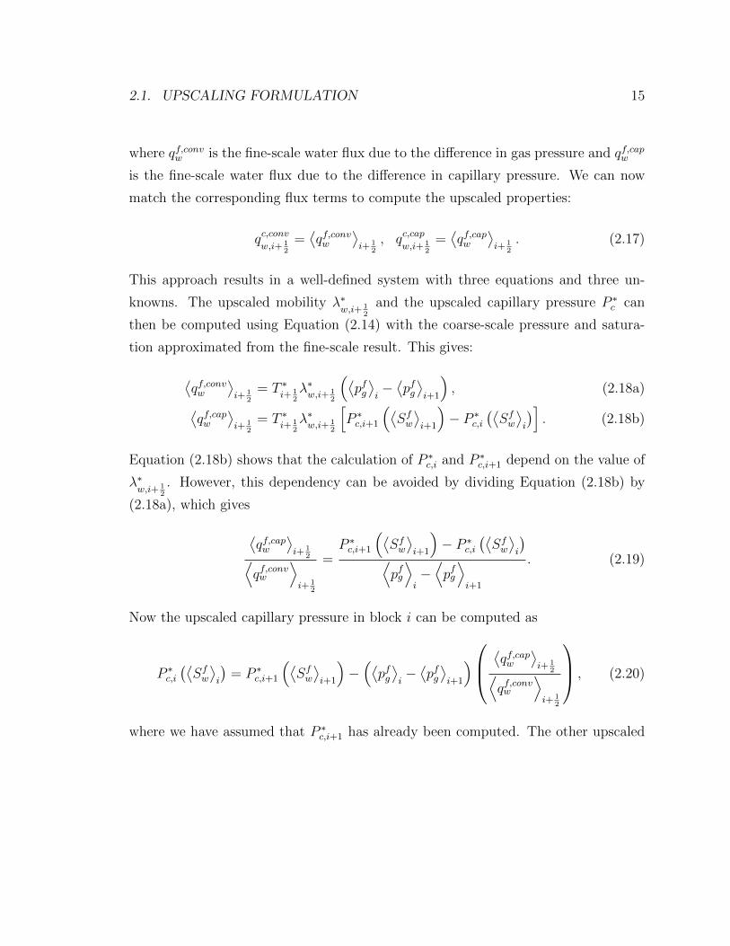
2.1. UPSCALING FORMULATION 15
where qf,convw is the fine-scale water flux due to the difference in gas pressure and qf,capw
is the fine-scale water flux due to the difference in capillary pressure. We can now
match the corresponding flux terms to compute the upscaled properties:
qc,convw,i+ 1
2
=⟨qf,convw
⟩i+ 1
2
, qc,capw,i+ 1
2
=⟨qf,capw
⟩i+ 1
2
. (2.17)
This approach results in a well-defined system with three equations and three un-
knowns. The upscaled mobility λ∗w,i+ 1
2
and the upscaled capillary pressure P ∗c can
then be computed using Equation (2.14) with the coarse-scale pressure and satura-
tion approximated from the fine-scale result. This gives:
⟨qf,convw
⟩i+ 1
2
= T ∗i+ 1
2λ∗w,i+ 1
2
(⟨pfg⟩i−⟨pfg⟩i+1
), (2.18a)
⟨qf,capw
⟩i+ 1
2
= T ∗i+ 1
2λ∗w,i+ 1
2
[P ∗c,i+1
(⟨Sfw⟩i+1
)− P ∗
c,i
(⟨Sfw⟩i
)]. (2.18b)
Equation (2.18b) shows that the calculation of P ∗c,i and P ∗
c,i+1 depend on the value of
λ∗w,i+ 1
2
. However, this dependency can be avoided by dividing Equation (2.18b) by
(2.18a), which gives
⟨qf,capw
⟩i+ 1
2⟨qf,convw
⟩i+ 1
2
=P ∗c,i+1
(⟨Sfw⟩i+1
)− P ∗
c,i
(⟨Sfw⟩i
)⟨pfg⟩i−⟨pfg⟩i+1
. (2.19)
Now the upscaled capillary pressure in block i can be computed as
P ∗c,i
(⟨Sfw⟩i
)= P ∗
c,i+1
(⟨Sfw⟩i+1
)−(⟨pfg⟩i−⟨pfg⟩i+1
)
⟨qf,capw
⟩i+ 1
2⟨qf,convw
⟩i+ 1
2
, (2.20)
where we have assumed that P ∗c,i+1 has already been computed. The other upscaled
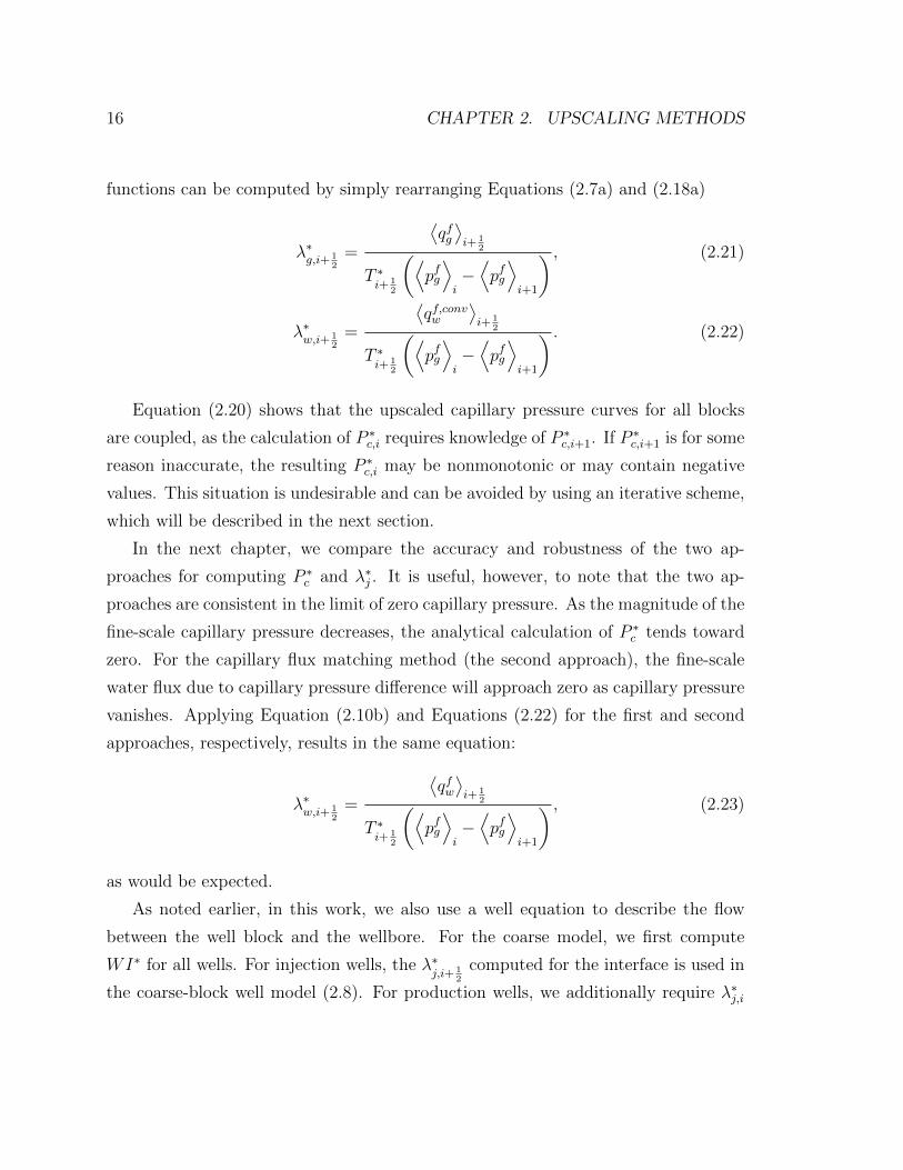
16 CHAPTER 2. UPSCALING METHODS
functions can be computed by simply rearranging Equations (2.7a) and (2.18a)
λ∗g,i+ 1
2=
⟨qfg⟩i+ 1
2
T ∗i+ 1
2
(⟨pfg⟩i−⟨pfg⟩i+1
) , (2.21)
λ∗w,i+ 1
2=
⟨qf,convw
⟩i+ 1
2
T ∗i+ 1
2
(⟨pfg⟩i−⟨pfg⟩i+1
) . (2.22)
Equation (2.20) shows that the upscaled capillary pressure curves for all blocks
are coupled, as the calculation of P ∗c,i requires knowledge of P ∗
c,i+1. If P ∗c,i+1 is for some
reason inaccurate, the resulting P ∗c,i may be nonmonotonic or may contain negative
values. This situation is undesirable and can be avoided by using an iterative scheme,
which will be described in the next section.
In the next chapter, we compare the accuracy and robustness of the two ap-
proaches for computing P ∗c and λ∗j . It is useful, however, to note that the two ap-
proaches are consistent in the limit of zero capillary pressure. As the magnitude of the
fine-scale capillary pressure decreases, the analytical calculation of P ∗c tends toward
zero. For the capillary flux matching method (the second approach), the fine-scale
water flux due to capillary pressure difference will approach zero as capillary pressure
vanishes. Applying Equation (2.10b) and Equations (2.22) for the first and second
approaches, respectively, results in the same equation:
λ∗w,i+ 1
2=
⟨qfw⟩i+ 1
2
T ∗i+ 1
2
(⟨pfg⟩i−⟨pfg⟩i+1
) , (2.23)
as would be expected.
As noted earlier, in this work, we also use a well equation to describe the flow
between the well block and the wellbore. For the coarse model, we first compute
WI∗ for all wells. For injection wells, the λ∗j,i+ 1
2
computed for the interface is used in
the coarse-block well model (2.8). For production wells, we additionally require λ∗j,i
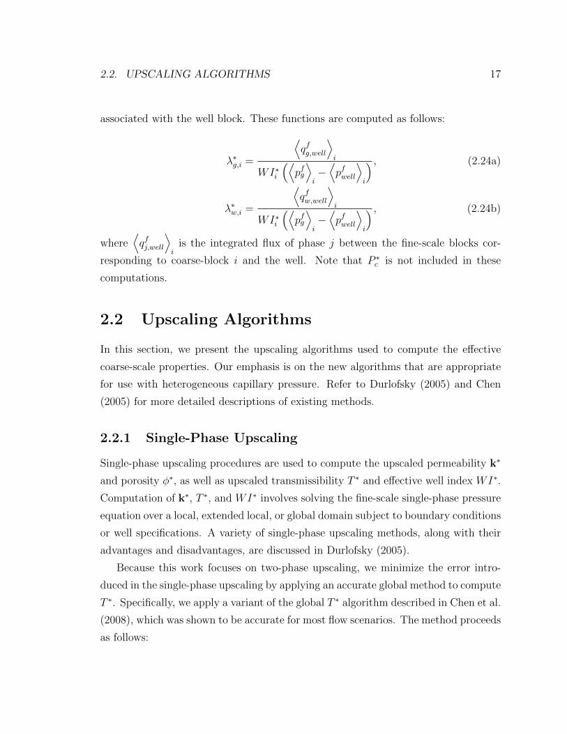
2.2. UPSCALING ALGORITHMS 17
associated with the well block. These functions are computed as follows:
λ∗g,i =
⟨qfg,well
⟩i
WI∗i
(⟨pfg⟩i−⟨pfwell
⟩i
) , (2.24a)
λ∗w,i =
⟨qfw,well
⟩i
WI∗i
(⟨pfg⟩i−⟨pfwell
⟩i
) , (2.24b)
where⟨qfj,well
⟩i
is the integrated flux of phase j between the fine-scale blocks cor-
responding to coarse-block i and the well. Note that P ∗c is not included in these
computations.
2.2 Upscaling Algorithms
In this section, we present the upscaling algorithms used to compute the effective
coarse-scale properties. Our emphasis is on the new algorithms that are appropriate
for use with heterogeneous capillary pressure. Refer to Durlofsky (2005) and Chen
(2005) for more detailed descriptions of existing methods.
2.2.1 Single-Phase Upscaling
Single-phase upscaling procedures are used to compute the upscaled permeability k∗
and porosity φ∗, as well as upscaled transmissibility T ∗ and effective well index WI∗.
Computation of k∗, T ∗, and WI∗ involves solving the fine-scale single-phase pressure
equation over a local, extended local, or global domain subject to boundary conditions
or well specifications. A variety of single-phase upscaling methods, along with their
advantages and disadvantages, are discussed in Durlofsky (2005).
Because this work focuses on two-phase upscaling, we minimize the error intro-
duced in the single-phase upscaling by applying an accurate global method to compute
T ∗. Specifically, we apply a variant of the global T ∗ algorithm described in Chen et al.
(2008), which was shown to be accurate for most flow scenarios. The method proceeds
as follows:
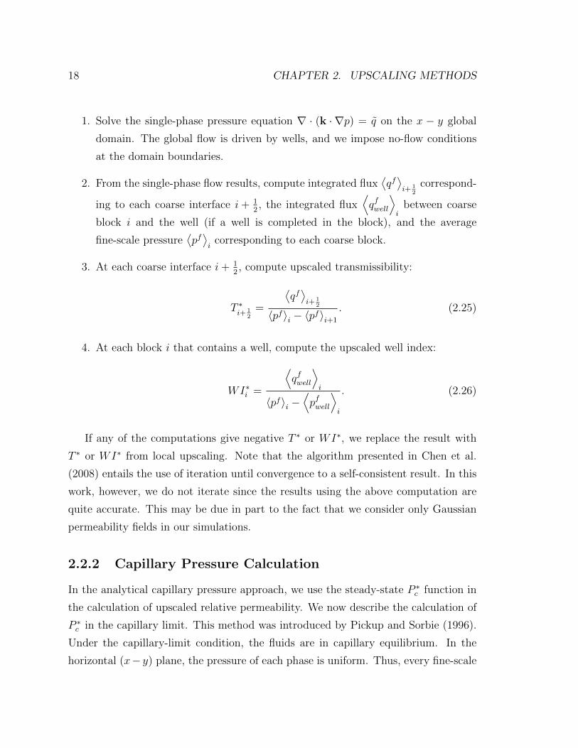
18 CHAPTER 2. UPSCALING METHODS
1. Solve the single-phase pressure equation ∇ · (k · ∇p) = q on the x − y global
domain. The global flow is driven by wells, and we impose no-flow conditions
at the domain boundaries.
2. From the single-phase flow results, compute integrated flux⟨qf⟩i+ 1
2
correspond-
ing to each coarse interface i+ 12, the integrated flux
⟨qfwell
⟩i
between coarse
block i and the well (if a well is completed in the block), and the average
fine-scale pressure⟨pf⟩i
corresponding to each coarse block.
3. At each coarse interface i+ 12, compute upscaled transmissibility:
T ∗i+ 1
2=
⟨qf⟩i+ 1
2
〈pf〉i − 〈pf〉i+1
. (2.25)
4. At each block i that contains a well, compute the upscaled well index:
WI∗i =
⟨qfwell
⟩i
〈pf〉i −⟨pfwell
⟩i
. (2.26)
If any of the computations give negative T ∗ or WI∗, we replace the result with
T ∗ or WI∗ from local upscaling. Note that the algorithm presented in Chen et al.
(2008) entails the use of iteration until convergence to a self-consistent result. In this
work, however, we do not iterate since the results using the above computation are
quite accurate. This may be due in part to the fact that we consider only Gaussian
permeability fields in our simulations.
2.2.2 Capillary Pressure Calculation
In the analytical capillary pressure approach, we use the steady-state P ∗c function in
the calculation of upscaled relative permeability. We now describe the calculation of
P ∗c in the capillary limit. This method was introduced by Pickup and Sorbie (1996).
Under the capillary-limit condition, the fluids are in capillary equilibrium. In the
horizontal (x− y) plane, the pressure of each phase is uniform. Thus, every fine-scale

2.2. UPSCALING ALGORITHMS 19
block within the target coarse block has the same capillary pressure, but the fluid
saturations are discontinuous. The method to compute upscaled capillary pressure
under the capillary-limit condition is as follows:
1. Over a target coarse block, determine the minimum possible capillary pressure
Pc,min and maximum possible capillary pressure Pc,max of the corresponding
fine-scale blocks.
2. For each fine-scale block k, invert the capillary pressure-saturation relationship;
i.e., compute Sw,k(Pc) (in practice, Pc for each fine block might be described by
a J−function, as discussed below).
3. For each capillary pressure level Pc within the range [Pc,min, Pc,max], we compute
average water saturation Scw from:
Scw(Pc) =
∑Nf
k=1 φkVkSw,k(Pc)∑Nf
k=1 φkVk, (2.27)
In this work, we consider φk and Vk to be constant, so the calculation for the
average water saturation reduces to:
Scw(Pc) =1
Nf
Nf∑
k=1
Sw,k(Pc). (2.28)
4. Record the resulting average saturation and capillary pressure (Scw, Pc) as a data
point for the capillary pressure curve P ∗c (Scw) of the coarse-scale block.
This approach is depicted in Figures 2.2 and 2.3.
The upscaled capillary pressured computed from the capillary-limit condition is
exact at vanishing fluid velocities, where the fluids are in capillary equilibrium. In our
work, although the capillary-limiting conditions are not fully satisfied, as we model
an injection process, the fluid velocity is sufficiently low such that the computed
upscaled capillary pressure should be reasonably accurate. In the regions of the
model where the fluid velocity is relatively high, the capillary-limit upscaled capillary

20 CHAPTER 2. UPSCALING METHODS
(a) Permeability (log scale) of the nine fine-scale blocks comprising the target coarseblock
0 0.2 0.4 0.6 0.8 10
10
20
30
40
50
Pc(psi)
Sw
(b) Pc curve for each fine-scale block
(c) Water saturation at Pc =10 psi
0 0.2 0.4 0.6 0.8 10
10
20
30
40
50
Pc
(psi
)
Sw
mean Sw = 0.3776
(d) Sw at Pc =10 psi
(e) Water saturation at Pc =20 psi
0 0.2 0.4 0.6 0.8 10
10
20
30
40
50
Pc
(psi
)
Sw
mean Sw = 0.2344
(f) Sw at Pc =20 psi
Figure 2.2: Schematic showing capillary pressure upscaling under the assumption ofcapillary-limit and steady-state conditions.
2.2. UPSCALING ALGORITHMS 21
0 0.2 0.4 0.6 0.8 10
10
20
30
40
50
Swc
Pc*(psi)
Figure 2.3: Resuting upscaled capillary pressure curve. Red circles show (Scw, P∗c )
pairs shown in Figure 2.2.
pressure may lose accuracy. However, the contribution of capillary pressure is smaller
at higher velocities, and the relative permeability correction largely compensates for
the inaccuracy in the upscaled capillary pressure.
2.2.3 Iterative Global Upscaling Method
In this section, we present a detailed description of the iterative global method for
upscaling two-phase properties, which was developed in this work. The method ex-
tends the approach for iterative global upscaling of T ∗, which was developed by Chen
et al. (2008).
We first describe the method for the case where P ∗c is computed in the capillary
limit. We perform a global fine-scale two-phase flow simulation. From this simulation,
we record the integrated water rate⟨qfw⟩i+ 1
2
and gas rate⟨qfg⟩i+ 1
2
for each coarse
interface i+ 12
as functions of the average water saturation⟨Sfw⟩i
of the upstream
block. Here,⟨Sfw⟩i
is computed using Equation (2.12) or (2.13), as appropriate. The
integrated flux functions are stored as functions which we designate as Fw,i+ 12(Sw)
and Fg,i+ 12(Sw). For blocks that contain producers, we record the integrated fluxes

22 CHAPTER 2. UPSCALING METHODS
0
1
2
3
4
5
6
7
8
0 0.1 0.2 0.3 0.4 0.5 0.6
Flux
thr
ough
coa
rse
inte
rfac
e
Sw
Water flux Gas flux
(a) Smooth flux profile
0
1
2
3
4
5
6
0 0.1 0.2 0.3 0.4 0.5 0.6
Flux
thr
ough
coa
rse
inte
rfac
e
Sw
Water flux Gas flux
(b) Noisy flux profile
Figure 2.4: Examples of water and gas flow rates as functions of upstream averagewater saturation. The flux profiles at some interfaces are generally smooth (a), whileothers can be noisy (b).
from the block to the wellbore⟨qfw,well
⟩i
and⟨qfg,well
⟩i. The fluxes are stored as
Fw,well,i(Sw) and Fg,well,i(Sw).
Examples of interface fluxes as functions of upstream water saturation are shown
in Figure 2.4. At the flow rates which are considered in this work, the resulting
Fw,i+ 12(Sw) and Fg,i+ 1
2(Sw) may be noisy; i.e., they may exhibit fluctuations (Figure
2.4b). As an optional step, we can apply a smoothing method to reduce or eliminate
the noise. In this work, we apply locally weighted linear regression, which will be
discussed later in this chapter.
We also compute the average fine-scale gas pressure⟨pfg⟩i
from Equation (2.11).
As the first step of the global upscaling procedure, the initial estimates for the up-
scaled mobility of the water and gas phases, λ∗w,i+ 1
2
and λ∗g,i+ 1
2
, are computed from
the fine-scale solutions using Equations (2.10a) and (2.10b). The resulting λ∗g,i+ 1
2
and
λ∗w,i+ 1
2
are stored as functions of the average fine-scale water saturation of the up-
stream block (i or i + 1). For the blocks with producers, we apply Equations (2.24)
to compute the upscaled mobility λ∗j,i.
2.2. UPSCALING ALGORITHMS 23
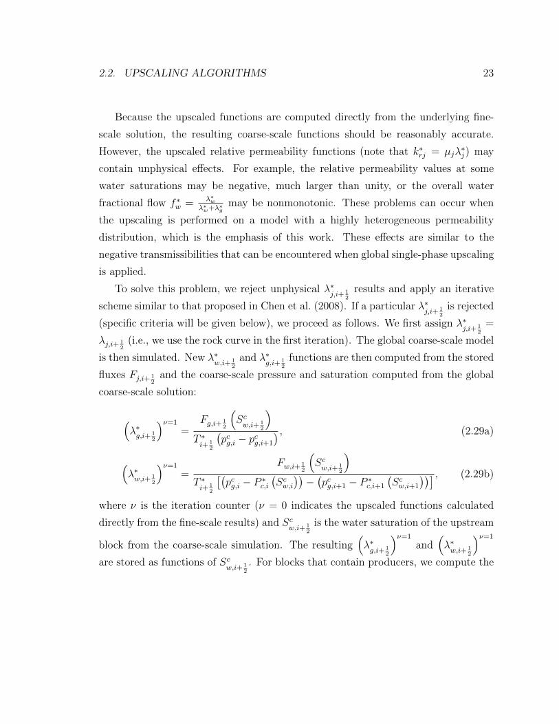
Because the upscaled functions are computed directly from the underlying fine-
scale solution, the resulting coarse-scale functions should be reasonably accurate.
However, the upscaled relative permeability functions (note that k∗rj = µjλ∗j) may
contain unphysical effects. For example, the relative permeability values at some
water saturations may be negative, much larger than unity, or the overall water
fractional flow f ∗w = λ∗w
λ∗w+λ∗gmay be nonmonotonic. These problems can occur when
the upscaling is performed on a model with a highly heterogeneous permeability
distribution, which is the emphasis of this work. These effects are similar to the
negative transmissibilities that can be encountered when global single-phase upscaling
is applied.
To solve this problem, we reject unphysical λ∗j,i+ 1
2
results and apply an iterative
scheme similar to that proposed in Chen et al. (2008). If a particular λ∗j,i+ 1
2
is rejected
(specific criteria will be given below), we proceed as follows. We first assign λ∗j,i+ 1
2
=
λj,i+ 12
(i.e., we use the rock curve in the first iteration). The global coarse-scale model
is then simulated. New λ∗w,i+ 1
2
and λ∗g,i+ 1
2
functions are then computed from the stored
fluxes Fj,i+ 12
and the coarse-scale pressure and saturation computed from the global
coarse-scale solution:
(λ∗g,i+ 1
2
)ν=1
=Fg,i+ 1
2
(Scw,i+ 1
2
)
T ∗i+ 1
2
(pcg,i − pcg,i+1
) , (2.29a)
(λ∗w,i+ 1
2
)ν=1
=Fw,i+ 1
2
(Scw,i+ 1
2
)
T ∗i+ 1
2
[(pcg,i − P ∗
c,i
(Scw,i
))−(pcg,i+1 − P ∗
c,i+1
(Scw,i+1
))] , (2.29b)
where ν is the iteration counter (ν = 0 indicates the upscaled functions calculated
directly from the fine-scale results) and Scw,i+ 1
2
is the water saturation of the upstream
block from the coarse-scale simulation. The resulting(λ∗g,i+ 1
2
)ν=1
and(λ∗w,i+ 1
2
)ν=1
are stored as functions of Scw,i+ 1
2
. For blocks that contain producers, we compute the
24 CHAPTER 2. UPSCALING METHODS
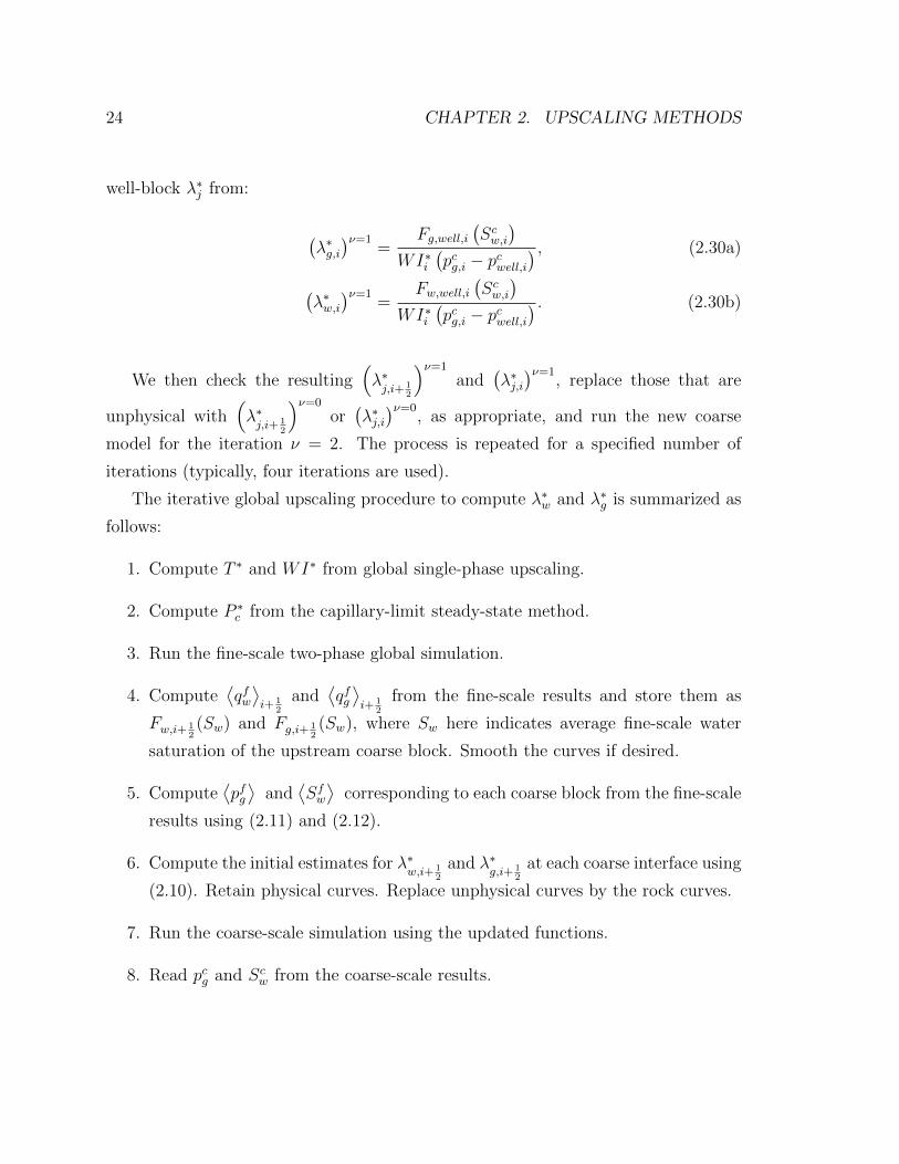
well-block λ∗j from:
(λ∗g,i)ν=1
=Fg,well,i
(Scw,i
)
WI∗i(pcg,i − pcwell,i
) , (2.30a)
(λ∗w,i)ν=1
=Fw,well,i
(Scw,i
)
WI∗i(pcg,i − pcwell,i
) . (2.30b)
We then check the resulting(λ∗j,i+ 1
2
)ν=1
and(λ∗j,i)ν=1
, replace those that are
unphysical with(λ∗j,i+ 1
2
)ν=0
or(λ∗j,i)ν=0
, as appropriate, and run the new coarse
model for the iteration ν = 2. The process is repeated for a specified number of
iterations (typically, four iterations are used).
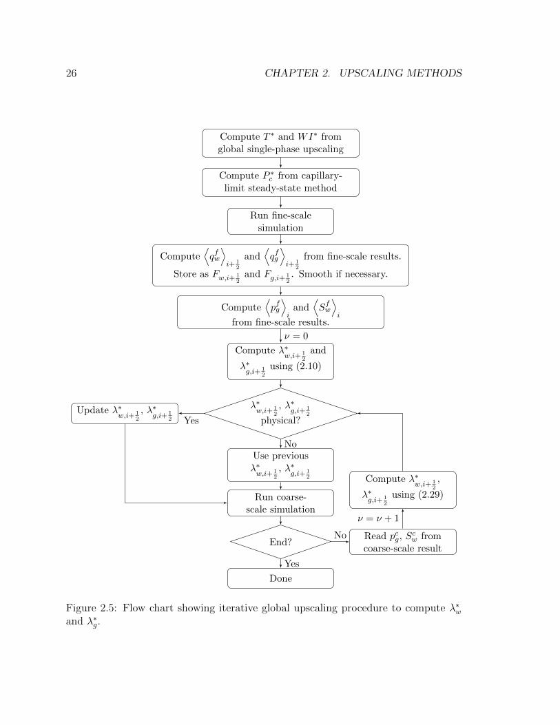
The iterative global upscaling procedure to compute λ∗w and λ∗g is summarized as
follows:
1. Compute T ∗ and WI∗ from global single-phase upscaling.
2. Compute P ∗c from the capillary-limit steady-state method.
3. Run the fine-scale two-phase global simulation.
4. Compute⟨qfw⟩i+ 1
2
and⟨qfg⟩i+ 1
2
from the fine-scale results and store them as
Fw,i+ 12(Sw) and Fg,i+ 1
2(Sw), where Sw here indicates average fine-scale water
saturation of the upstream coarse block. Smooth the curves if desired.
5. Compute⟨pfg⟩
and⟨Sfw⟩
corresponding to each coarse block from the fine-scale
results using (2.11) and (2.12).
6. Compute the initial estimates for λ∗w,i+ 1
2
and λ∗g,i+ 1
2
at each coarse interface using
(2.10). Retain physical curves. Replace unphysical curves by the rock curves.
7. Run the coarse-scale simulation using the updated functions.
8. Read pcg and Scw from the coarse-scale results.
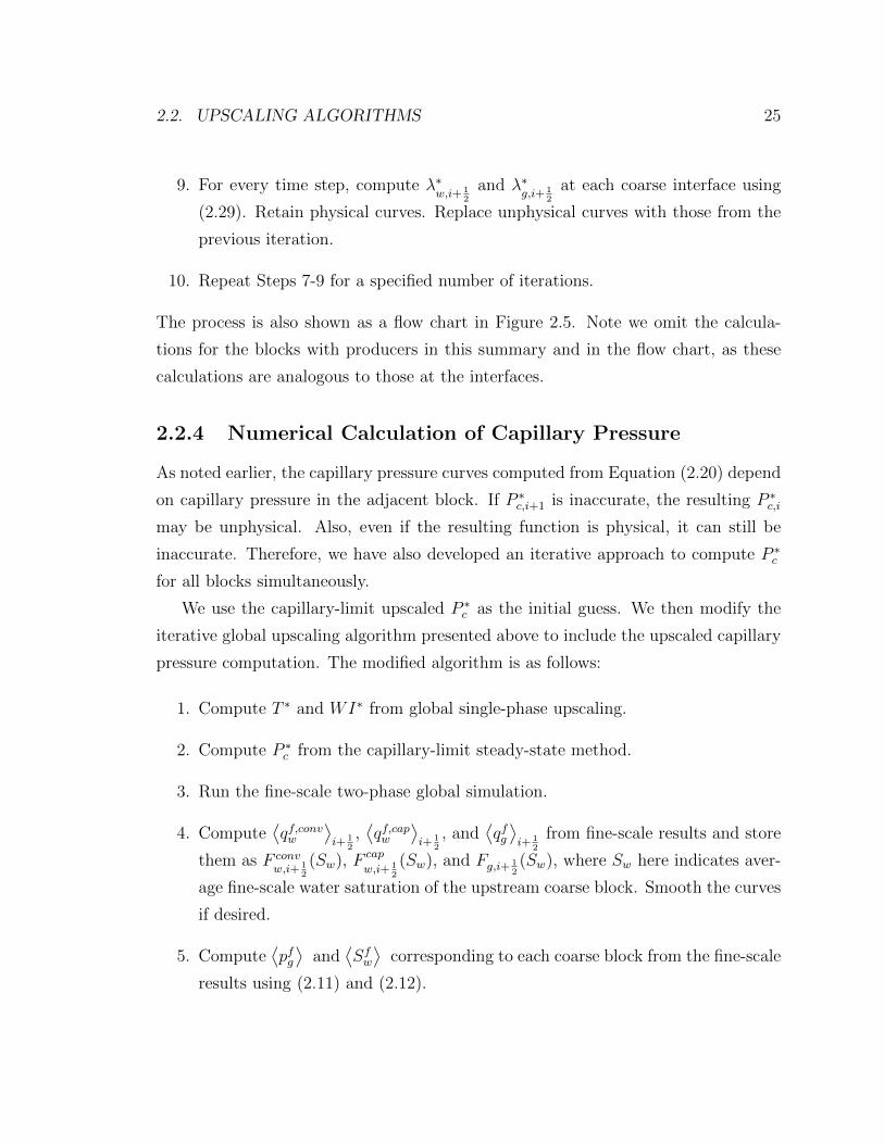
2.2. UPSCALING ALGORITHMS 25
9. For every time step, compute λ∗w,i+ 1
2
and λ∗g,i+ 1
2
at each coarse interface using
(2.29). Retain physical curves. Replace unphysical curves with those from the
previous iteration.
10. Repeat Steps 7-9 for a specified number of iterations.
The process is also shown as a flow chart in Figure 2.5. Note we omit the calcula-
tions for the blocks with producers in this summary and in the flow chart, as these
calculations are analogous to those at the interfaces.
2.2.4 Numerical Calculation of Capillary Pressure
As noted earlier, the capillary pressure curves computed from Equation (2.20) depend
on capillary pressure in the adjacent block. If P ∗c,i+1 is inaccurate, the resulting P ∗
c,i
may be unphysical. Also, even if the resulting function is physical, it can still be
inaccurate. Therefore, we have also developed an iterative approach to compute P ∗c
for all blocks simultaneously.
We use the capillary-limit upscaled P ∗c as the initial guess. We then modify the
iterative global upscaling algorithm presented above to include the upscaled capillary
pressure computation. The modified algorithm is as follows:
1. Compute T ∗ and WI∗ from global single-phase upscaling.
2. Compute P ∗c from the capillary-limit steady-state method.
3. Run the fine-scale two-phase global simulation.
4. Compute⟨qf,convw
⟩i+ 1
2
,⟨qf,capw
⟩i+ 1
2
, and⟨qfg⟩i+ 1
2
from fine-scale results and store
them as F convw,i+ 1
2
(Sw), F cap
w,i+ 12
(Sw), and Fg,i+ 12(Sw), where Sw here indicates aver-
age fine-scale water saturation of the upstream coarse block. Smooth the curves
if desired.
5. Compute⟨pfg⟩
and⟨Sfw⟩
corresponding to each coarse block from the fine-scale
results using (2.11) and (2.12).
26 CHAPTER 2. UPSCALING METHODS
Compute T ∗ and WI∗ fromglobal single-phase upscaling
Compute P ∗c from capillary-
limit steady-state method
Run fine-scalesimulation
Compute⟨qfw⟩i+ 1
2
and⟨qfg⟩i+ 1
2
from fine-scale results.
Store as Fw,i+ 12
and Fg,i+ 12. Smooth if necessary.
Compute⟨pfg⟩i
and⟨Sfw
⟩i
from fine-scale results.
Compute λ∗w,i+ 1
2
and
λ∗g,i+ 1
2
using (2.10)
λ∗w,i+ 1
2
, λ∗g,i+ 1
2
physical?Update λ∗
w,i+ 12
, λ∗g,i+ 1
2
Use previousλ∗w,i+ 1
2
, λ∗g,i+ 1
2
Run coarse-scale simulation
End?
Done
Read pcg, Scw from
coarse-scale result
Compute λ∗w,i+ 1
2
,
λ∗g,i+ 1
2
using (2.29)
ν = 0
Yes
No
Yes
No
ν = ν + 1
Figure 2.5: Flow chart showing iterative global upscaling procedure to compute λ∗wand λ∗g.
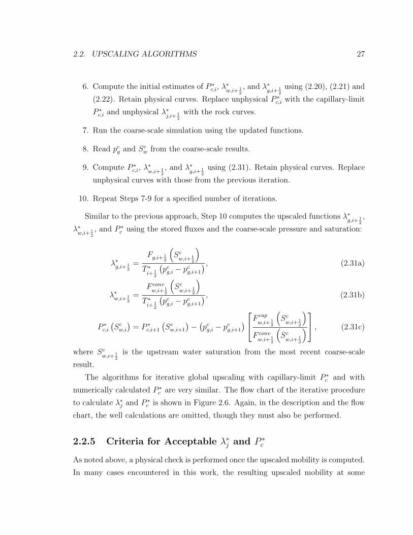
2.2. UPSCALING ALGORITHMS 27
6. Compute the initial estimates of P ∗c,i, λ
∗w,i+ 1
2
, and λ∗g,i+ 1
2
using (2.20), (2.21) and
(2.22). Retain physical curves. Replace unphysical P ∗c,i with the capillary-limit
P ∗c,i and unphysical λ∗
j,i+ 12
with the rock curves.
7. Run the coarse-scale simulation using the updated functions.
8. Read pcg and Scw from the coarse-scale results.
9. Compute P ∗c,i, λ
∗w,i+ 1
2
, and λ∗g,i+ 1
2
using (2.31). Retain physical curves. Replace
unphysical curves with those from the previous iteration.
10. Repeat Steps 7-9 for a specified number of iterations.
Similar to the previous approach, Step 10 computes the upscaled functions λ∗g,i+ 1
2
,
λ∗w,i+ 1
2
, and P ∗c using the stored fluxes and the coarse-scale pressure and saturation:
λ∗g,i+ 1
2=
Fg,i+ 12
(Scw,i+ 1
2
)
T ∗i+ 1
2
(pcg,i − pcg,i+1
) , (2.31a)
λ∗w,i+ 1
2=
F convw,i+ 1
2
(Scw,i+ 1
2
)
T ∗i+ 1
2
(pcg,i − pcg,i+1
) , (2.31b)
P ∗c,i
(Scw,i
)= P ∗
c,i+1
(Scw,i+1
)−(pcg,i − pcg,i+1
)F cap
w,i+ 12
(Scw,i+ 1
2
)
F convw,i+ 1
2
(Scw,i+ 1
2
)
, (2.31c)
where Scw,i+ 1
2
is the upstream water saturation from the most recent coarse-scale
result.
The algorithms for iterative global upscaling with capillary-limit P ∗c and with
numerically calculated P ∗c are very similar. The flow chart of the iterative procedure
to calculate λ∗j and P ∗c is shown in Figure 2.6. Again, in the description and the flow
chart, the well calculations are omitted, though they must also be performed.
2.2.5 Criteria for Acceptable λ∗j and P ∗c
As noted above, a physical check is performed once the upscaled mobility is computed.
In many cases encountered in this work, the resulting upscaled mobility at some
28 CHAPTER 2. UPSCALING METHODS
Compute T ∗ and WI∗ fromglobal single-phase upscaling
Compute P ∗c from capillary-
limit steady-state method
Run fine-scalesimulation
Compute⟨qf,convw
⟩i+ 1
2
,⟨qf,capw
⟩i+ 1
2
and⟨qfg⟩i+ 1
2
from fine-scale
results. Store as F convw,i+ 1
2
, F cap
w,i+ 12
, and Fg,i+ 12. Smooth if necessary.
Compute⟨pfg⟩i
and⟨Sfw
⟩i
from fine-scale results.
Compute P ∗c,i, λ
∗w,i+ 1
2
and λ∗g,i+ 1
2
using (2.20), (2.21), (2.22)
P ∗c,i, λ
∗w,i+ 1
2
,
λ∗g,i+ 1
2
physical?
Update P ∗c,i,
λ∗w,i+ 1
2
, λ∗g,i+ 1
2
Use previous P ∗c,i,
λ∗w,i+ 1
2
, λ∗g,i+ 1
2
Run coarse-scale simulation
End?
Done
Read pcg, Scw from
coarse-scale result
Compute P ∗c,i, λ
∗w,i+ 1
2
,
λ∗g,i+ 1
2
using (2.31)
ν = 0
Yes
No
Yes
No
ν = ν + 1
Figure 2.6: Flow chart showing iterative global upscaling procedure to compute λ∗w,λ∗g, and P ∗
c . Shaded blocks indicates modifications from Figure 2.5.
2.3. OTHER METHODS AND ISSUES 29
saturation may be negative, or the upscaled relative permeability (calculated from
k∗rj = µjλ∗j) may be much greater than unity. This situation occurs especially when
the flow rates are low. In this work, we retain upscaled functions that satisfy
min(k∗rj)≥ 0, max
(k∗rj)≤ 2. (2.32)
We also require that the water fractional flow increases as water saturation in-
creases. In the absence of capillary pressure effects, this leads to the condition
df ∗w
dScw≥ 0, (2.33)
where f ∗w = λ∗w
λ∗w+λ∗gis the fractional flow of water. However, with capillary pressure
effects, f ∗w depends on both phase mobilities and capillary pressure difference. We
find that requiring f ∗w to be a monotonically increasing function of Scw is an overly
restrictive condition, as the effects of capillary pressure are not accounted for. In this
work, we apply the following condition
df ∗w
dScw≥ −0.2, (2.34)
which allows a slight decrease in f ∗w. If (2.32) or (2.34) are not satisfied, we reject
the updated function and use the upscaled function from the previous iteration (or
the rock curves if the function has never been updated). Note that our treatment
here will reject both of the updated λ∗j,i+ 1
2
if either λ∗w,i+ 1
2
or λ∗g,i+ 1
2
is found to be
unphysical based on the criteria above.
2.3 Other Methods and Issues
2.3.1 Smoothing
As shown in Figure 2.4, the gas and water fluxes at some interfaces are generally
smooth, while the fluxes at other interfaces may display oscillations. In our numerical
tests, oscillatory fluxes often occur when the flow is capillary-dominated, i.e., the flow
30 CHAPTER 2. UPSCALING METHODS
rate is low. These fluxes may cause unphysical results when they are used in the
iterative upscaling scheme.
To remove this effect, we apply locally weighted linear regression for smoothing.
The locally weighted linear regression model assumes that the data,(Sw, Fw,i+ 1
2
)
or(Sw, Fg,i+ 1
2
)in our case, can be fitted locally by straight lines. In the following
description of the locally weighted linear regression, we use the notation (x, y) as
generic independent and dependent variables, respectively. This description follows
the discussion in Ng (2012). Around a location x, we approximate the value of y as
a straight line such that
y = θ1x+ θ0, (2.35)
or in a vector notation
y = hθ(x) = θTx, (2.36)
where θ = [θ1 θ0]T and x = [x 1]T . The goal of the locally weighted linear regression
is to find the parameter θ to minimize the weighted square error between the straight
line and the data
θ = arg minθ
m∑
j=1
wj(θTxj − yj
)2, (2.37)
where xj = [xj 1]T , (xj, yj) is a data point, wj is the weight of each data point, and
m is the total number of data points. Solving the optimization problem, which is
similar to the ordinary least square, a closed-form solution of the optimal parameter
θ is obtained as
θ = (XTWX)−1XTWy, (2.38)
where
X =
x1 1
x2 1...
...
xm 1
, y =
y1
y2
...
ym
, W =
w1
w2
. . .
wm
. (2.39)
Note that because we fit a local straight line to each location x, the optimal parameter
2.3. OTHER METHODS AND ISSUES 31
θ changes as a function of x. The local weight wj is usually taken as
wj = exp
(−(xj − x)2
2τ 2
), (2.40)
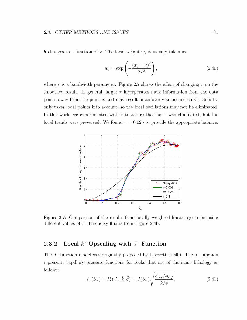
where τ is a bandwidth parameter. Figure 2.7 shows the effect of changing τ on the
smoothed result. In general, larger τ incorporates more information from the data
points away from the point x and may result in an overly smoothed curve. Small τ
only takes local points into account, so the local oscillations may not be eliminated.
In this work, we experimented with τ to assure that noise was eliminated, but the
local trends were preserved. We found τ = 0.025 to provide the appropriate balance.
0 0.1 0.2 0.3 0.4 0.5 0.60
1
2
3
4
5
6
Upstream Swc
Gas
flux
thro
ugh
coar
se in
terf
ace
Noisy data
τ=0.005
τ=0.025
τ=0.1
Figure 2.7: Comparison of the results from locally weighted linear regression usingdifferent values of τ . The noisy flux is from Figure 2.4b.
2.3.2 Local k∗ Upscaling with J−Function
The J−function model was originally proposed by Leverett (1940). The J−function
represents capillary pressure functions for rocks that are of the same lithology as
follows:
Pc(Sw) = Pc(Sw, k, φ) = J(Sw)
√kref/φref
k/φ, (2.41)
32 CHAPTER 2. UPSCALING METHODS
where kref is a reference permeability, φref is the reference porosity, and k and φ are
the permeability and porosity of the rock (grid block in our case) of interest. The
J(Sw) function is considered to be given for a particular lithology.
An alternative approach to assigning P ∗c , based on the use of J(Sw), was suggested
by Saadatpoor et al. (2011). Essentially, the coarse blocks were assumed to share the
same J−function as the fine-scale block, which gives
P ∗c (Scw) = Pc(S
cw, k, φ
∗) = J(Scw)
√kref/φref
k/φ∗. (2.42)
Here, k is the upscaled permeability, φ∗ is the upscaled porosity, and J(Scw) is the
same as the fine-scale J−function.
Saadatpoor et al. (2011) used a simple geometric average of the fine-scale perme-
ability to compute the coarse-scale k. In this work, however, we apply local upscaling
for the target coarse-block with standard boundary conditions (constant pressure at
the inlet and outlet and no-flow conditions elsewhere) to compute k∗x, k∗y, and k∗z .
The permeability value used in the J−function is the geometric average of these
three permeability values
k = 3
√k∗xk
∗yk
∗z . (2.43)
Using this k seems more appropriate than simply using the geometric average of the
fine-scale permeability, as it incorporates some flow behavior into the construction of
P ∗c . We do not compare results using this treatment with results using the treatment
of Saadatpoor et al. (2011), as both approaches are considered to be quite approxi-
mate.
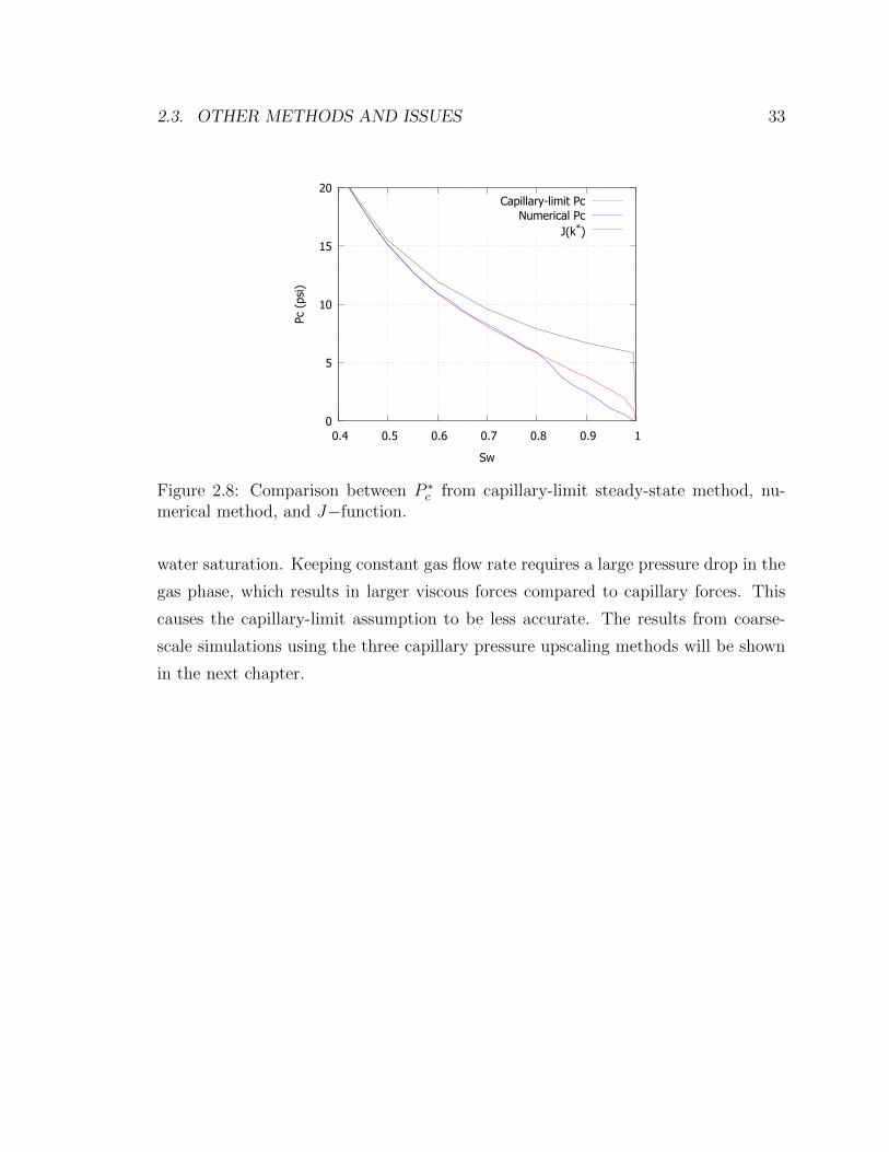
The resulting P ∗c computed from the J−function method, the capillary-limit
steady-state method, and the numerical scheme are compared in Figure 2.8. We
see that the upscaled capillary pressure using the J−function is significantly different
from the capillary-limit P ∗c and the numerically computed P ∗
c , while the capillary-
limit P ∗c and the numerically computed P ∗
c are very close to each other for Sw ≤ 0.8.
The capillary-limit P ∗c and numerically computed P ∗
c differ at high water saturation
for many curves computed in this work. This is because the gas mobility is low at high
2.3. OTHER METHODS AND ISSUES 33
0
5
10
15
20
0.4 0.5 0.6 0.7 0.8 0.9 1
Pc (
psi)
Sw
Capillary-limit PcNumerical Pc
J(k*)
Figure 2.8: Comparison between P ∗c from capillary-limit steady-state method, nu-
merical method, and J−function.
water saturation. Keeping constant gas flow rate requires a large pressure drop in the
gas phase, which results in larger viscous forces compared to capillary forces. This
causes the capillary-limit assumption to be less accurate. The results from coarse-
scale simulations using the three capillary pressure upscaling methods will be shown
in the next chapter.

34 CHAPTER 2. UPSCALING METHODS
Chapter 3
Numerical Results
In this chapter, we apply the two-phase upscaling procedures to a synthetic reservoir
model. We assess both the accuracy and robustness of the upscaling methods. In the
accuracy assessment, we compare the results from coarse-scale simulations to results
from the corresponding fine-scale simulation. In the robustness assessment, coarse
models based on the global upscaling of one specific case are applied for cases with
different flow rates or well locations.
3.1 Model Construction
In this section, we describe the reservoir models used in this study. The discus-
sion covers the permeability fields, rock and fluid properties, and well locations and
controls.
3.1.1 Reservoir Model
The reservoir models used in the study are two-dimensional systems containing 200×100 grid blocks (in the x− and y−directions, respectively). The size of each block is
2 ft× 1 ft. The rock is taken to be incompressible and of uniform porosity (φ = 0.25)
throughout the reservoir. The permeability distribution is generated using Sequential
Gaussian Simulation (Deutsch and Journel, 1992) with the parameters shown in Table
35
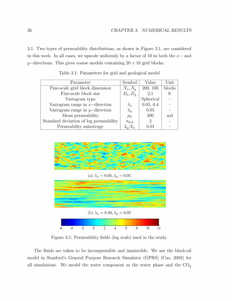
36 CHAPTER 3. NUMERICAL RESULTS
3.1. Two types of permeability distributions, as shown in Figure 3.1, are considered
in this work. In all cases, we upscale uniformly by a factor of 10 in both the x− and
y−directions. This gives coarse models containing 20× 10 grid blocks.
Table 3.1: Parameters for grid and geological model
Parameter Symbol Value UnitFine-scale grid block dimension Nx, Ny 200, 100 blocks
Fine-scale block size Dx, Dy 2,1 ftVariogram type Spherical -
Variogram range in x−direction λx 0.05, 0.4 -Variogram range in y−direction λy 0.05 -
Mean permeability µk 200 mdStandard deviation of log permeability σln k 2 -
Permeability anisotropy ky/kx 0.01 -
(a) λx = 0.05, λy = 0.05
(b) λx = 0.40, λy = 0.05
Figure 3.1: Permeability fields (log scale) used in the study.
The fluids are taken to be incompressible and immiscible. We use the black-oil
model in Stanford’s General Purpose Research Simulator (GPRS) (Cao, 2002) for
all simulations. We model the water component as the water phase and the CO2
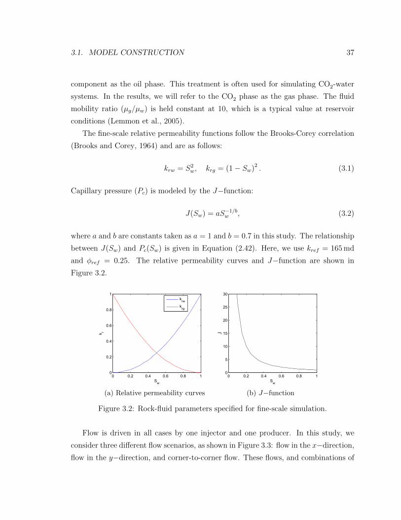
3.1. MODEL CONSTRUCTION 37
component as the oil phase. This treatment is often used for simulating CO2-water
systems. In the results, we will refer to the CO2 phase as the gas phase. The fluid
mobility ratio (µg/µw) is held constant at 10, which is a typical value at reservoir
conditions (Lemmon et al., 2005).
The fine-scale relative permeability functions follow the Brooks-Corey correlation
(Brooks and Corey, 1964) and are as follows:
krw = S2w, krg = (1− Sw)2 . (3.1)
Capillary pressure (Pc) is modeled by the J−function:
J(Sw) = aS−1/bw , (3.2)
where a and b are constants taken as a = 1 and b = 0.7 in this study. The relationship
between J(Sw) and Pc(Sw) is given in Equation (2.42). Here, we use kref = 165 md
and φref = 0.25. The relative permeability curves and J−function are shown in
Figure 3.2.
0 0.2 0.4 0.6 0.8 10
0.2
0.4
0.6
0.8
1
Sw
k r
krw
krg
(a) Relative permeability curves
0 0.2 0.4 0.6 0.8 10
5
10
15
20
25
30
J, k
ref=
165
md
Sw
J
(b) J−function
Figure 3.2: Rock-fluid parameters specified for fine-scale simulation.
Flow is driven in all cases by one injector and one producer. In this study, we
consider three different flow scenarios, as shown in Figure 3.3: flow in the x−direction,
flow in the y−direction, and corner-to-corner flow. These flows, and combinations of
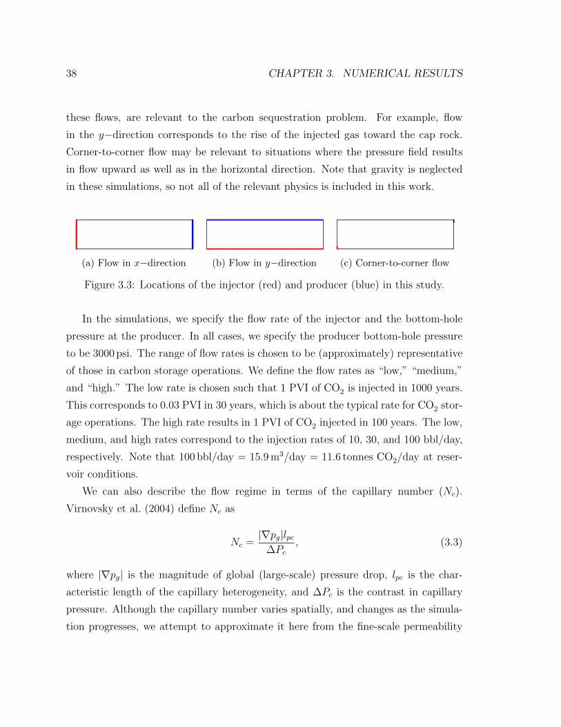
38 CHAPTER 3. NUMERICAL RESULTS
these flows, are relevant to the carbon sequestration problem. For example, flow
in the y−direction corresponds to the rise of the injected gas toward the cap rock.
Corner-to-corner flow may be relevant to situations where the pressure field results
in flow upward as well as in the horizontal direction. Note that gravity is neglected
in these simulations, so not all of the relevant physics is included in this work.
(a) Flow in x−direction (b) Flow in y−direction (c) Corner-to-corner flow
Figure 3.3: Locations of the injector (red) and producer (blue) in this study.
In the simulations, we specify the flow rate of the injector and the bottom-hole
pressure at the producer. In all cases, we specify the producer bottom-hole pressure
to be 3000 psi. The range of flow rates is chosen to be (approximately) representative
of those in carbon storage operations. We define the flow rates as “low,” “medium,”
and “high.” The low rate is chosen such that 1 PVI of CO2 is injected in 1000 years.
This corresponds to 0.03 PVI in 30 years, which is about the typical rate for CO2 stor-
age operations. The high rate results in 1 PVI of CO2 injected in 100 years. The low,
medium, and high rates correspond to the injection rates of 10, 30, and 100 bbl/day,
respectively. Note that 100 bbl/day = 15.9 m3/day = 11.6 tonnes CO2/day at reser-
voir conditions.
We can also describe the flow regime in terms of the capillary number (Nc).
Virnovsky et al. (2004) define Nc as
Nc =|∇pg|lpc
∆Pc, (3.3)
where |∇pg| is the magnitude of global (large-scale) pressure drop, lpc is the char-
acteristic length of the capillary heterogeneity, and ∆Pc is the contrast in capillary
pressure. Although the capillary number varies spatially, and changes as the simula-
tion progresses, we attempt to approximate it here from the fine-scale permeability
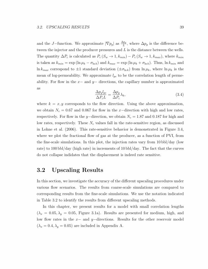
3.2. UPSCALING RESULTS 39
and the J−function. We approximate |∇pg| as ∆pgL
, where ∆pg is the difference be-
tween the injector and the producer pressures and L is the distance between the wells.
The quantity ∆Pc is calculated as Pc (Sw → 1, kmin)− Pc (Sw → 1, kmax), where kmin
is taken as kmin = exp (lnµk − σln k) and kmax = exp (lnµk + σln k). Thus, ln kmin and
ln kmax correspond to ±1 standard deviation (±σln k) from lnµk, where lnµk is the
mean of log-permeability. We approximate lpc to be the correlation length of perme-
ability. For flow in the x− and y− directions, the capillary number is approximated
as∆pglpc∆PcL
=∆pg∆Pc
λk, (3.4)
where k = x, y corresponds to the flow direction. Using the above approximation,
we obtain Nc = 0.67 and 0.067 for flow in the x−direction with high and low rates,
respectively. For flow in the y−direction, we obtain Nc = 1.87 and 0.187 for high and
low rates, respectively. These Nc values fall in the rate-sensitive region, as discussed
in Lohne et al. (2006). This rate-sensitive behavior is demonstrated in Figure 3.4,
where we plot the fractional flow of gas at the producer, as a function of PVI, from
the fine-scale simulations. In this plot, the injection rates vary from 10 bbl/day (low
rate) to 100 bbl/day (high rate) in increments of 10 bbl/day. The fact that the curves
do not collapse indidates that the displacement is indeed rate sensitive.
3.2 Upscaling Results
In this section, we investigate the accuracy of the different upscaling procedures under
various flow scenarios. The results from coarse-scale simulations are compared to
corresponding results from the fine-scale simulations. We use the notation indicated
in Table 3.2 to identify the results from different upscaling methods.
In this chapter, we present results for a model with small correlation lengths
(λx = 0.05, λy = 0.05, Figure 3.1a). Results are presented for medium, high, and
low flow rates in the x− and y−directions. Results for the other reservoir model
(λx = 0.4, λy = 0.05) are included in Appendix A.
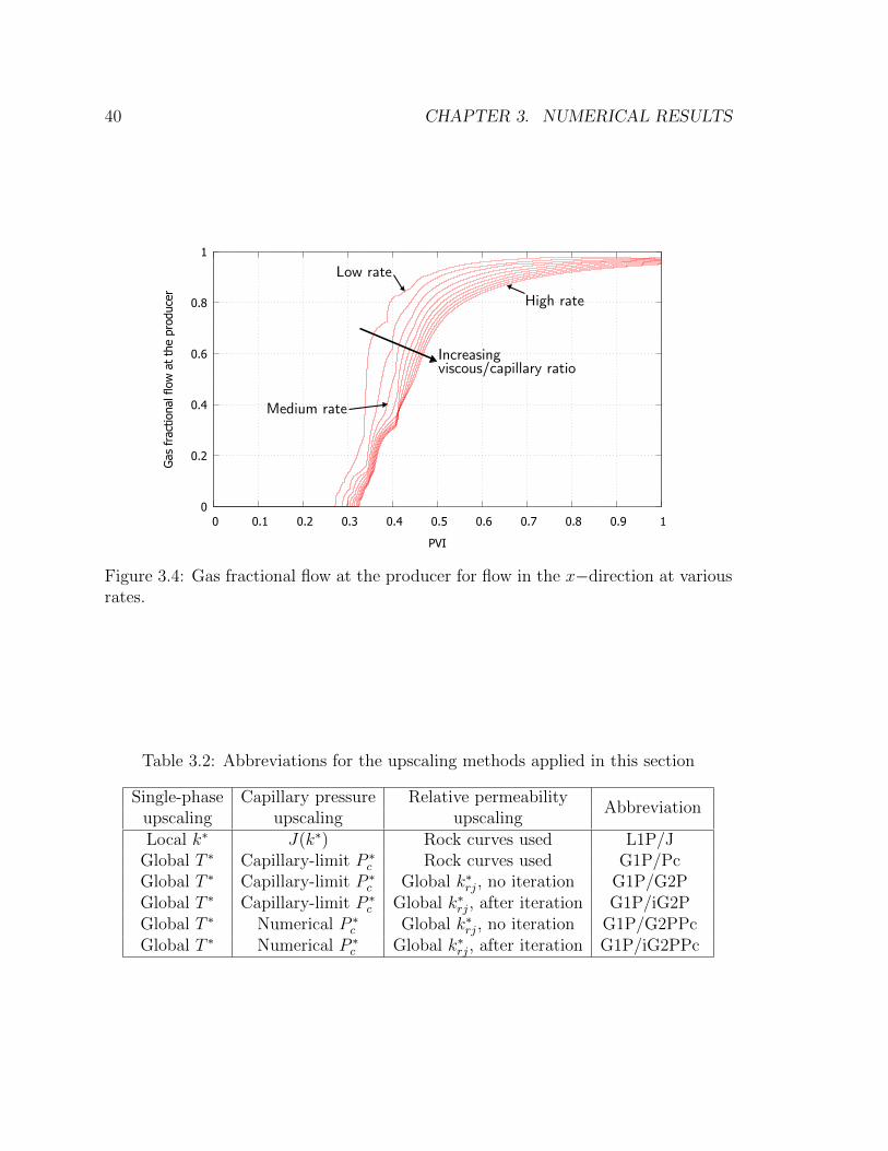
40 CHAPTER 3. NUMERICAL RESULTS
0
0.2
0.4
0.6
0.8
1
0 0.1 0.2 0.3 0.4 0.5 0.6 0.7 0.8 0.9 1
Gas
fra
ctio
nal f
low
at
the
prod
ucer
PVI
Low rate
High rate
Medium rate
Increasing viscous/capillary ratio
Figure 3.4: Gas fractional flow at the producer for flow in the x−direction at variousrates.
Table 3.2: Abbreviations for the upscaling methods applied in this section
Single-phase Capillary pressure Relative permeabilityAbbreviation
upscaling upscaling upscalingLocal k∗ J(k∗) Rock curves used L1P/J
Global T ∗ Capillary-limit P ∗c Rock curves used G1P/Pc
Global T ∗ Capillary-limit P ∗c Global k∗rj, no iteration G1P/G2P
Global T ∗ Capillary-limit P ∗c Global k∗rj, after iteration G1P/iG2P
Global T ∗ Numerical P ∗c Global k∗rj, no iteration G1P/G2PPc
Global T ∗ Numerical P ∗c Global k∗rj, after iteration G1P/iG2PPc
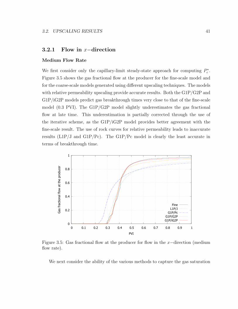
3.2. UPSCALING RESULTS 41
3.2.1 Flow in x−direction
Medium Flow Rate
We first consider only the capillary-limit steady-state approach for computing P ∗c .
Figure 3.5 shows the gas fractional flow at the producer for the fine-scale model and
for the coarse-scale models generated using different upscaling techniques. The models
with relative permeability upscaling provide accurate results. Both the G1P/G2P and
G1P/iG2P models predict gas breakthrough times very close to that of the fine-scale
model (0.3 PVI). The G1P/G2P model slightly underestimates the gas fractional
flow at late time. This underestimation is partially corrected through the use of
the iterative scheme, as the G1P/iG2P model provides better agreement with the
fine-scale result. The use of rock curves for relative permeability leads to inaccurate
results (L1P/J and G1P/Pc). The G1P/Pc model is clearly the least accurate in
terms of breakthrough time.
0
0.2
0.4
0.6
0.8
1
0 0.1 0.2 0.3 0.4 0.5 0.6 0.7 0.8 0.9 1
Gas
fra
ctio
nal f
low
at
the
prod
ucer
PVI
FineL1P/J
G1P/PcG1P/G2PG1P/iG2P
Figure 3.5: Gas fractional flow at the producer for flow in the x−direction (mediumflow rate).
We next consider the ability of the various methods to capture the gas saturation
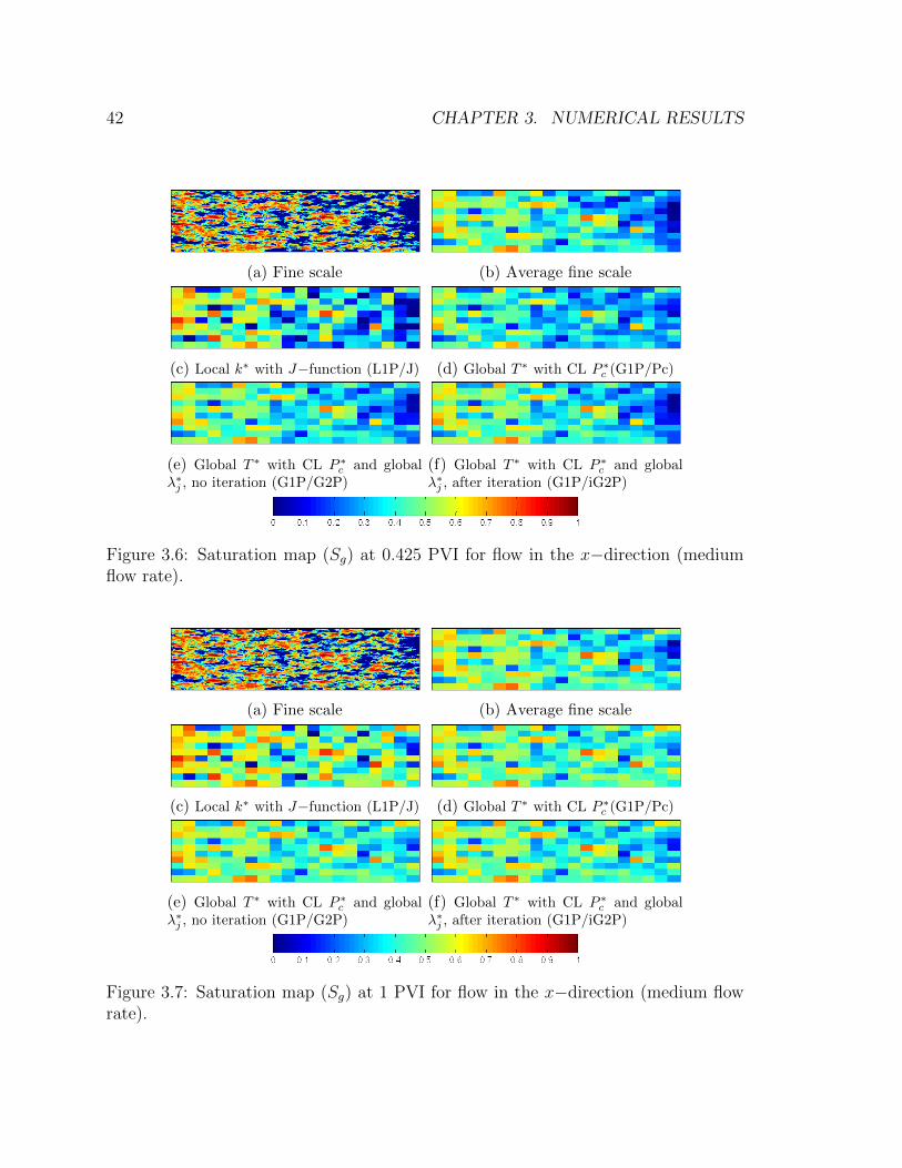
42 CHAPTER 3. NUMERICAL RESULTS
(a) Fine scale (b) Average fine scale
(c) Local k∗ with J−function (L1P/J) (d) Global T ∗ with CL P ∗c (G1P/Pc)
(e) Global T ∗ with CL P ∗c and global
λ∗j , no iteration (G1P/G2P)(f) Global T ∗ with CL P ∗
c and globalλ∗j , after iteration (G1P/iG2P)
Figure 3.6: Saturation map (Sg) at 0.425 PVI for flow in the x−direction (mediumflow rate).
(a) Fine scale (b) Average fine scale
(c) Local k∗ with J−function (L1P/J) (d) Global T ∗ with CL P ∗c (G1P/Pc)
(e) Global T ∗ with CL P ∗c and global
λ∗j , no iteration (G1P/G2P)(f) Global T ∗ with CL P ∗
c and globalλ∗j , after iteration (G1P/iG2P)
Figure 3.7: Saturation map (Sg) at 1 PVI for flow in the x−direction (medium flowrate).

3.2. UPSCALING RESULTS 43
throughout the reservoir. Figures 3.6a and 3.7a show the gas saturation from the fine-
scale simulation at 0.425 PVI and 1 PVI, and their corresponding volume-averaged
saturation distributions are shown in Figures 3.6b and 3.7b. The value of 0.425 PVI
is chosen to represent a time after significant gas breakthrough has occured, while 1
PVI represents the end of the simulation. Coarse-scale results should ideally match
the volume-averaged results. Qualitatively, we observe that the gas saturation from
the L1P/J model (Figures 3.6c and 3.7c) is more discontinuous than the averaged
fine-scale results and the other coarse-scale results at both 0.425 PVI and 1 PVI.
Detailed observation indicates that the G1P/G2P and G1P/iG2P saturation fields
are the most accurate compated to the averaged fine-scale results.
To more clearly quantify the inaccuracy in the gas saturation distribution, we
define the normalized L2−norm of the differences between the fine-scale and coarse-
scale results as:
e(t) =
∥∥Scg(t)−⟨Sfg (t)
⟩∥∥2∥∥∥
⟨Sfg (t)
⟩∥∥∥2
, (3.5)
where⟨Sfg (t)
⟩is the volume average of the fine-scale gas saturation corresponding to a
single coarse-scale block at dimensionless time t (defined in terms of PVI). The errors
e(t) are calculated at each simulation time and are plotted in Figure 3.8. To quantify
the time-averaged saturation error for each case, we define the overall saturation error
as
ET =1
tend
∫ tend
0
e(t)dt, (3.6)
where tend is the total dimensionless simulation time, which is 1 PVI for all cases
presented in this chapter.
As shown in Figure 3.8, L1P/J leads to the largest error in gas saturation at all
times. In addition, calculating upscaled relative permeability from the global solu-
tion (G1P/G2P) causes significant improvement from the case with capillary pres-
sure upscaling alone (G1P/Pc). The iterative scheme (G1P/iG2P) further improves
coarse-model accuracy. The overall saturation error of each model is shown in Table
3.3. These results are consistent with our observations above.
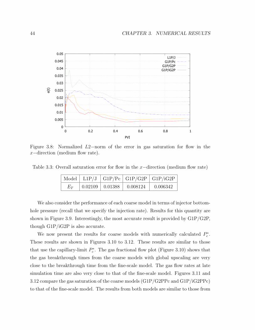
44 CHAPTER 3. NUMERICAL RESULTS
0
0.005
0.01
0.015
0.02
0.025
0.03
0.035
0.04
0.045
0.05
0 0.2 0.4 0.6 0.8 1
e(t)
PVI
L1P/JG1P/Pc
G1P/G2PG1P/iG2P
Figure 3.8: Normalized L2−norm of the error in gas saturation for flow in thex−direction (medium flow rate).
Table 3.3: Overall saturation error for flow in the x−direction (medium flow rate)
Model L1P/J G1P/Pc G1P/G2P G1P/iG2P
ET 0.02109 0.01388 0.008124 0.006342
We also consider the performance of each coarse model in terms of injector bottom-
hole pressure (recall that we specify the injection rate). Results for this quantity are
shown in Figure 3.9. Interestingly, the most accurate result is provided by G1P/G2P,
though G1P/iG2P is also accurate.
We now present the results for coarse models with numerically calculated P ∗c .
These results are shown in Figures 3.10 to 3.12. These results are similar to those
that use the capillary-limit P ∗c . The gas fractional flow plot (Figure 3.10) shows that
the gas breakthrough times from the coarse models with global upscaling are very
close to the breakthrough time from the fine-scale model. The gas flow rates at late
simulation time are also very close to that of the fine-scale model. Figures 3.11 and
3.12 compare the gas saturation of the coarse models (G1P/G2PPc and G1P/iG2PPc)
to that of the fine-scale model. The results from both models are similar to those from
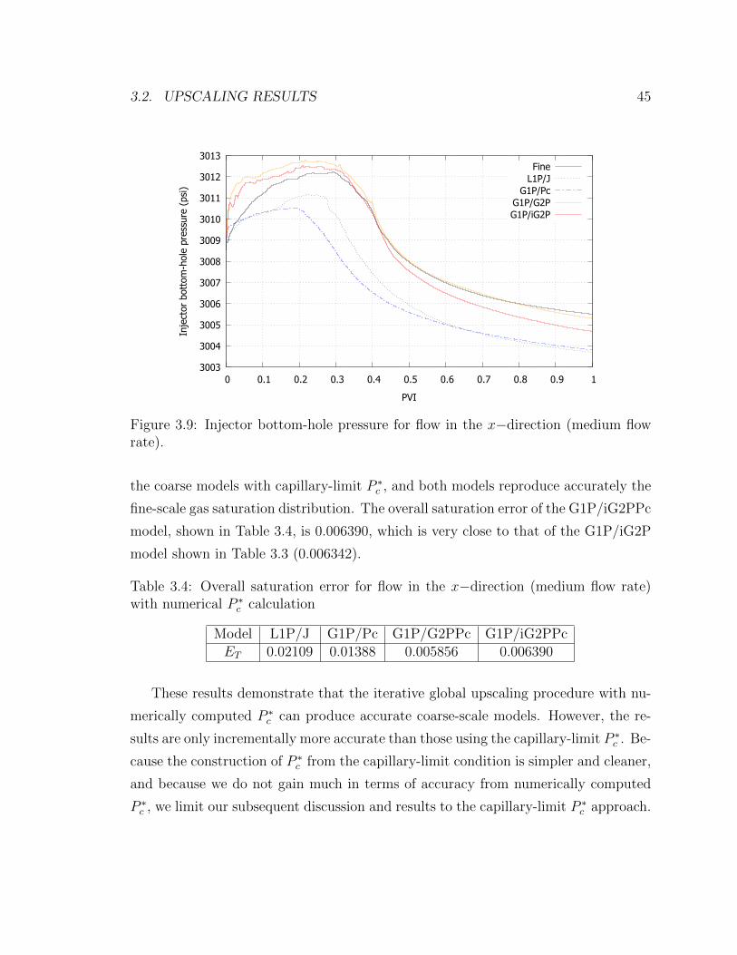
3.2. UPSCALING RESULTS 45
3003
3004
3005
3006
3007
3008
3009
3010
3011
3012
3013
0 0.1 0.2 0.3 0.4 0.5 0.6 0.7 0.8 0.9 1
Inje
ctor
bot
tom
-hol
e pr
essu
re (
psi)
PVI
FineL1P/J
G1P/PcG1P/G2PG1P/iG2P
Figure 3.9: Injector bottom-hole pressure for flow in the x−direction (medium flowrate).
the coarse models with capillary-limit P ∗c , and both models reproduce accurately the
fine-scale gas saturation distribution. The overall saturation error of the G1P/iG2PPc
model, shown in Table 3.4, is 0.006390, which is very close to that of the G1P/iG2P
model shown in Table 3.3 (0.006342).
Table 3.4: Overall saturation error for flow in the x−direction (medium flow rate)with numerical P ∗
c calculation
Model L1P/J G1P/Pc G1P/G2PPc G1P/iG2PPcET 0.02109 0.01388 0.005856 0.006390
These results demonstrate that the iterative global upscaling procedure with nu-
merically computed P ∗c can produce accurate coarse-scale models. However, the re-
sults are only incrementally more accurate than those using the capillary-limit P ∗c . Be-
cause the construction of P ∗c from the capillary-limit condition is simpler and cleaner,
and because we do not gain much in terms of accuracy from numerically computed
P ∗c , we limit our subsequent discussion and results to the capillary-limit P ∗
c approach.
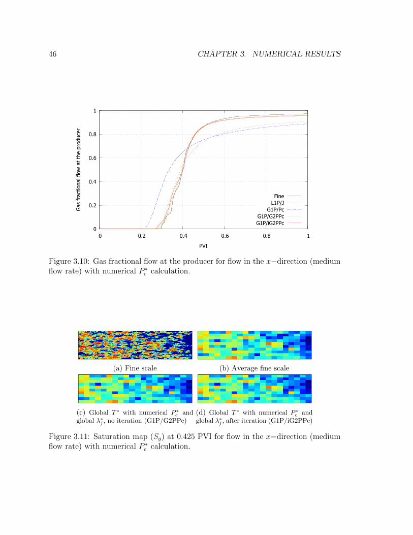
46 CHAPTER 3. NUMERICAL RESULTS
0
0.2
0.4
0.6
0.8
1
0 0.2 0.4 0.6 0.8 1
Gas
fra
ctio
nal f
low
at
the
prod
ucer
PVI
FineL1P/J
G1P/PcG1P/G2PPcG1P/iG2PPc
Figure 3.10: Gas fractional flow at the producer for flow in the x−direction (mediumflow rate) with numerical P ∗
c calculation.
(a) Fine scale (b) Average fine scale
(c) Global T ∗ with numerical P ∗c and
global λ∗j , no iteration (G1P/G2PPc)(d) Global T ∗ with numerical P ∗
c andglobal λ∗j , after iteration (G1P/iG2PPc)
Figure 3.11: Saturation map (Sg) at 0.425 PVI for flow in the x−direction (mediumflow rate) with numerical P ∗
c calculation.
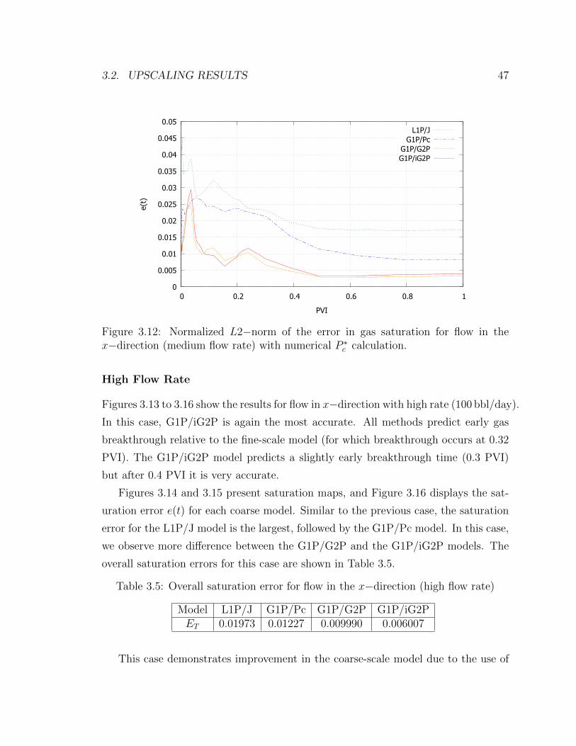
3.2. UPSCALING RESULTS 47
0
0.005
0.01
0.015
0.02
0.025
0.03
0.035
0.04
0.045
0.05
0 0.2 0.4 0.6 0.8 1
e(t)
PVI
L1P/JG1P/Pc
G1P/G2PG1P/iG2P
Figure 3.12: Normalized L2−norm of the error in gas saturation for flow in thex−direction (medium flow rate) with numerical P ∗
c calculation.
High Flow Rate
Figures 3.13 to 3.16 show the results for flow in x−direction with high rate (100 bbl/day).
In this case, G1P/iG2P is again the most accurate. All methods predict early gas
breakthrough relative to the fine-scale model (for which breakthrough occurs at 0.32
PVI). The G1P/iG2P model predicts a slightly early breakthrough time (0.3 PVI)
but after 0.4 PVI it is very accurate.
Figures 3.14 and 3.15 present saturation maps, and Figure 3.16 displays the sat-
uration error e(t) for each coarse model. Similar to the previous case, the saturation
error for the L1P/J model is the largest, followed by the G1P/Pc model. In this case,
we observe more difference between the G1P/G2P and the G1P/iG2P models. The
overall saturation errors for this case are shown in Table 3.5.
Table 3.5: Overall saturation error for flow in the x−direction (high flow rate)
Model L1P/J G1P/Pc G1P/G2P G1P/iG2PET 0.01973 0.01227 0.009990 0.006007
This case demonstrates improvement in the coarse-scale model due to the use of
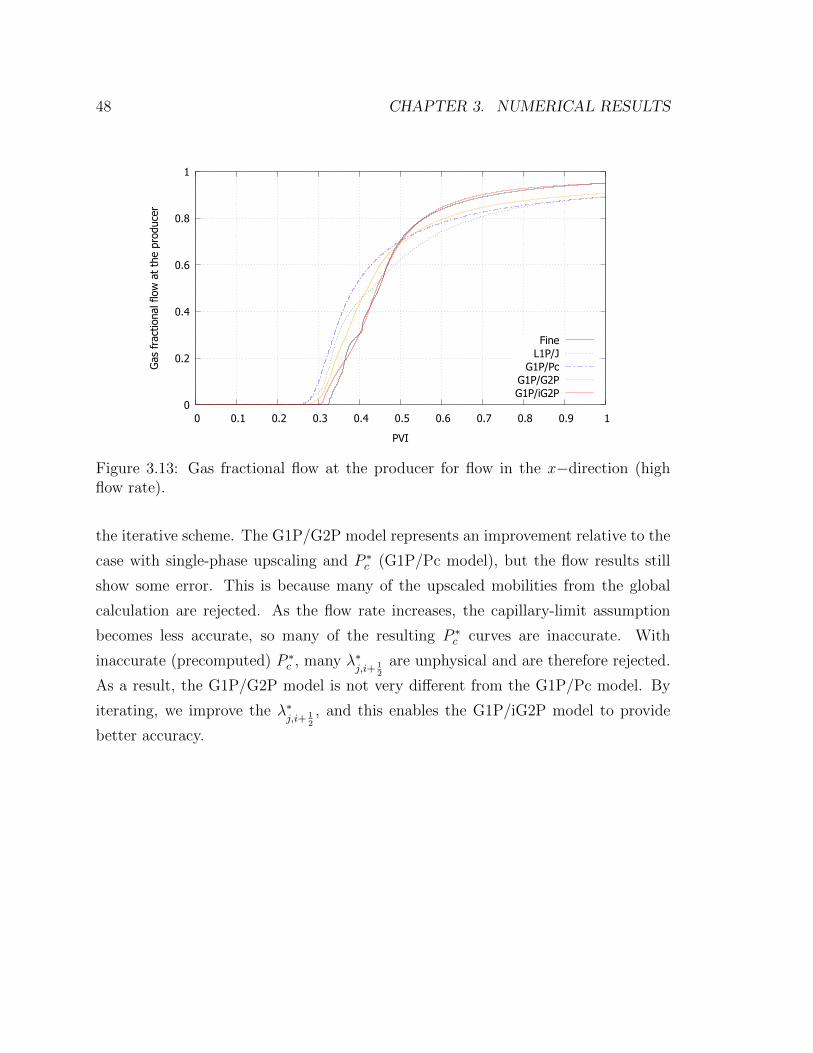
48 CHAPTER 3. NUMERICAL RESULTS
0
0.2
0.4
0.6
0.8
1
0 0.1 0.2 0.3 0.4 0.5 0.6 0.7 0.8 0.9 1
Gas
fra
ctio
nal f
low
at
the
prod
ucer
PVI
FineL1P/J
G1P/PcG1P/G2PG1P/iG2P
Figure 3.13: Gas fractional flow at the producer for flow in the x−direction (highflow rate).
the iterative scheme. The G1P/G2P model represents an improvement relative to the
case with single-phase upscaling and P ∗c (G1P/Pc model), but the flow results still
show some error. This is because many of the upscaled mobilities from the global
calculation are rejected. As the flow rate increases, the capillary-limit assumption
becomes less accurate, so many of the resulting P ∗c curves are inaccurate. With
inaccurate (precomputed) P ∗c , many λ∗
j,i+ 12
are unphysical and are therefore rejected.
As a result, the G1P/G2P model is not very different from the G1P/Pc model. By
iterating, we improve the λ∗j,i+ 1
2
, and this enables the G1P/iG2P model to provide
better accuracy.
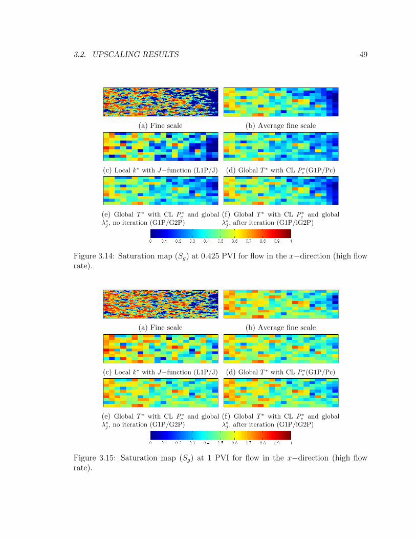
3.2. UPSCALING RESULTS 49
(a) Fine scale (b) Average fine scale
(c) Local k∗ with J−function (L1P/J) (d) Global T ∗ with CL P ∗c (G1P/Pc)
(e) Global T ∗ with CL P ∗c and global
λ∗j , no iteration (G1P/G2P)(f) Global T ∗ with CL P ∗
c and globalλ∗j , after iteration (G1P/iG2P)
Figure 3.14: Saturation map (Sg) at 0.425 PVI for flow in the x−direction (high flowrate).
(a) Fine scale (b) Average fine scale
(c) Local k∗ with J−function (L1P/J) (d) Global T ∗ with CL P ∗c (G1P/Pc)
(e) Global T ∗ with CL P ∗c and global
λ∗j , no iteration (G1P/G2P)(f) Global T ∗ with CL P ∗
c and globalλ∗j , after iteration (G1P/iG2P)
Figure 3.15: Saturation map (Sg) at 1 PVI for flow in the x−direction (high flowrate).
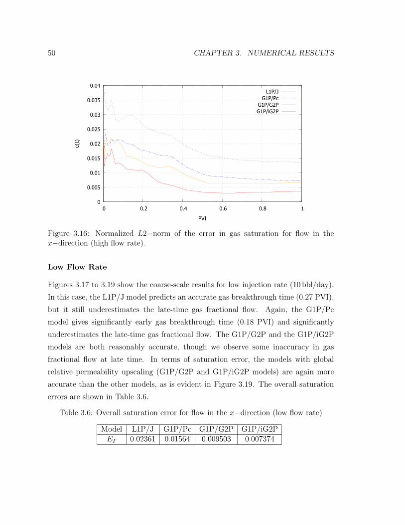
50 CHAPTER 3. NUMERICAL RESULTS
0
0.005
0.01
0.015
0.02
0.025
0.03
0.035
0.04
0 0.2 0.4 0.6 0.8 1
e(t)
PVI
L1P/JG1P/Pc
G1P/G2PG1P/iG2P
Figure 3.16: Normalized L2−norm of the error in gas saturation for flow in thex−direction (high flow rate).
Low Flow Rate
Figures 3.17 to 3.19 show the coarse-scale results for low injection rate (10 bbl/day).
In this case, the L1P/J model predicts an accurate gas breakthrough time (0.27 PVI),
but it still underestimates the late-time gas fractional flow. Again, the G1P/Pc
model gives significantly early gas breakthrough time (0.18 PVI) and significantly
underestimates the late-time gas fractional flow. The G1P/G2P and the G1P/iG2P
models are both reasonably accurate, though we observe some inaccuracy in gas
fractional flow at late time. In terms of saturation error, the models with global
relative permeability upscaling (G1P/G2P and G1P/iG2P models) are again more
accurate than the other models, as is evident in Figure 3.19. The overall saturation
errors are shown in Table 3.6.
Table 3.6: Overall saturation error for flow in the x−direction (low flow rate)
Model L1P/J G1P/Pc G1P/G2P G1P/iG2PET 0.02361 0.01564 0.009503 0.007374
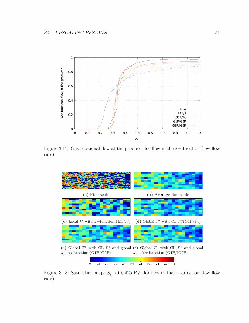
3.2. UPSCALING RESULTS 51
0
0.2
0.4
0.6
0.8
1
0 0.1 0.2 0.3 0.4 0.5 0.6 0.7 0.8 0.9 1
Gas
fra
ctio
nal f
low
at
the
prod
ucer
PVI
FineL1P/J
G1P/PcG1P/G2PG1P/iG2P
Figure 3.17: Gas fractional flow at the producer for flow in the x−direction (low flowrate).
(a) Fine scale (b) Average fine scale
(c) Local k∗ with J−function (L1P/J) (d) Global T ∗ with CL P ∗c (G1P/Pc)
(e) Global T ∗ with CL P ∗c and global
λ∗j , no iteration (G1P/G2P)(f) Global T ∗ with CL P ∗
c and globalλ∗j , after iteration (G1P/iG2P)
Figure 3.18: Saturation map (Sg) at 0.425 PVI for flow in the x−direction (low flowrate).
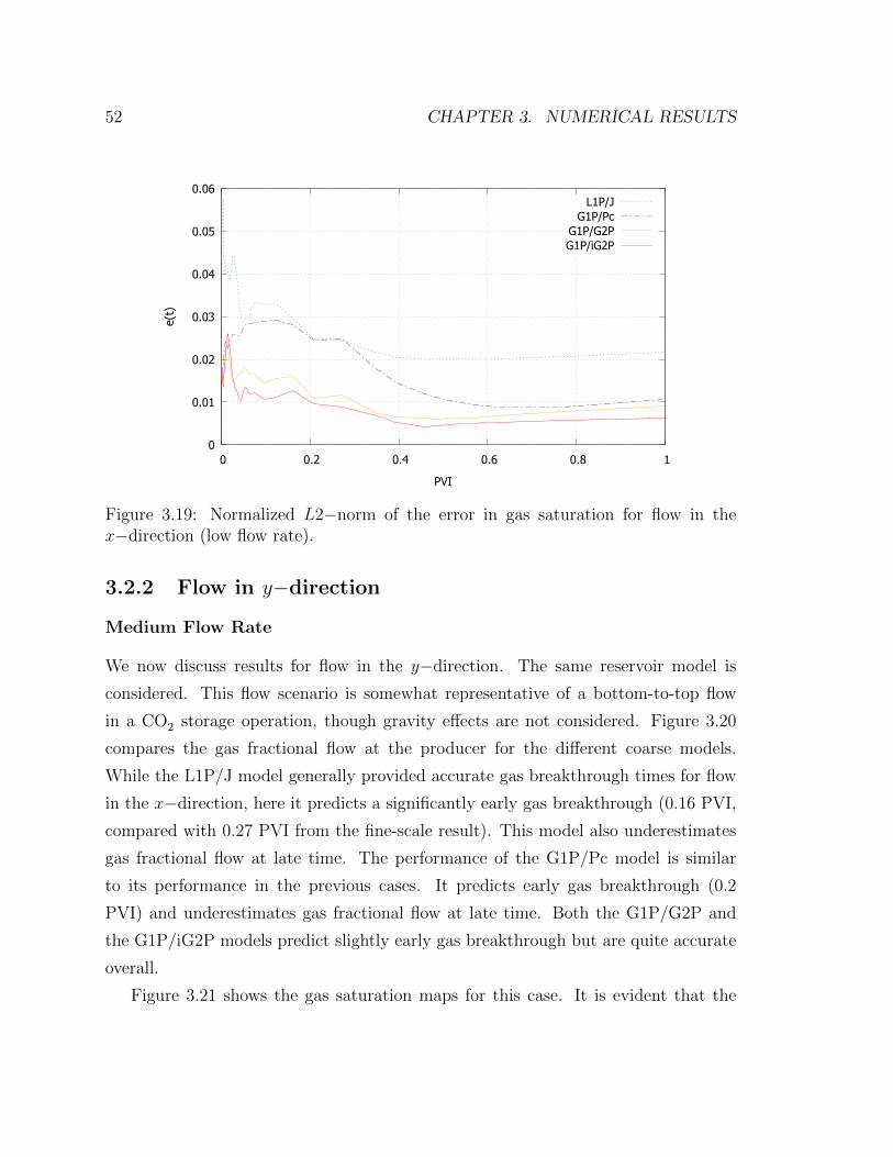
52 CHAPTER 3. NUMERICAL RESULTS
0
0.01
0.02
0.03
0.04
0.05
0.06
0 0.2 0.4 0.6 0.8 1
e(t)
PVI
L1P/JG1P/Pc
G1P/G2PG1P/iG2P
Figure 3.19: Normalized L2−norm of the error in gas saturation for flow in thex−direction (low flow rate).
3.2.2 Flow in y−direction
Medium Flow Rate
We now discuss results for flow in the y−direction. The same reservoir model is
considered. This flow scenario is somewhat representative of a bottom-to-top flow
in a CO2 storage operation, though gravity effects are not considered. Figure 3.20
compares the gas fractional flow at the producer for the different coarse models.
While the L1P/J model generally provided accurate gas breakthrough times for flow
in the x−direction, here it predicts a significantly early gas breakthrough (0.16 PVI,
compared with 0.27 PVI from the fine-scale result). This model also underestimates
gas fractional flow at late time. The performance of the G1P/Pc model is similar
to its performance in the previous cases. It predicts early gas breakthrough (0.2
PVI) and underestimates gas fractional flow at late time. Both the G1P/G2P and
the G1P/iG2P models predict slightly early gas breakthrough but are quite accurate
overall.
Figure 3.21 shows the gas saturation maps for this case. It is evident that the
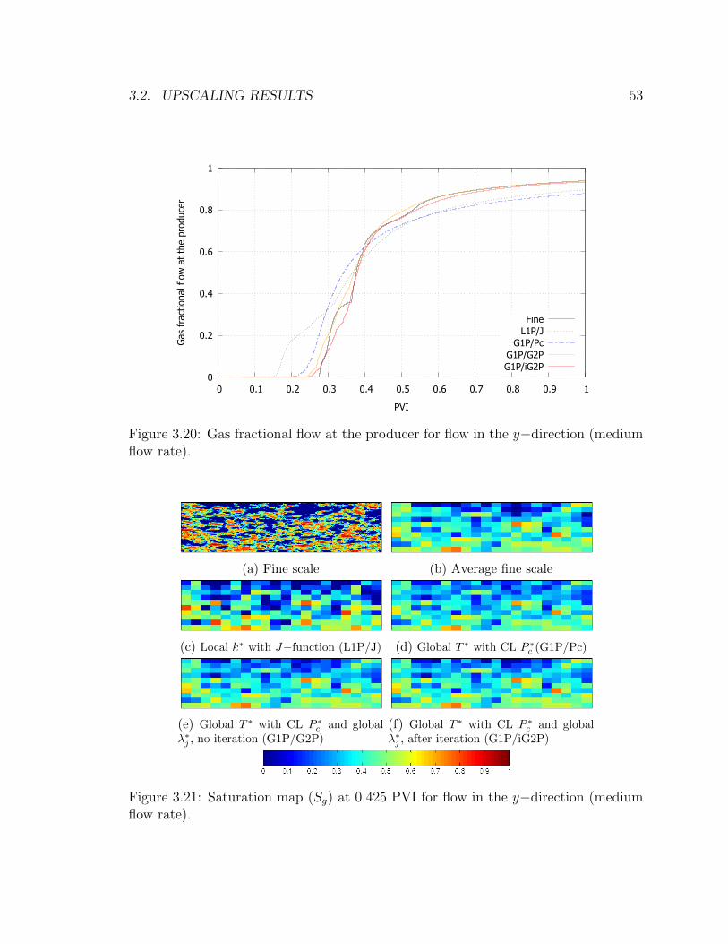
3.2. UPSCALING RESULTS 53
0
0.2
0.4
0.6
0.8
1
0 0.1 0.2 0.3 0.4 0.5 0.6 0.7 0.8 0.9 1
Gas
fra
ctio
nal f
low
at
the
prod
ucer
PVI
FineL1P/J
G1P/PcG1P/G2PG1P/iG2P
Figure 3.20: Gas fractional flow at the producer for flow in the y−direction (mediumflow rate).
(a) Fine scale (b) Average fine scale
(c) Local k∗ with J−function (L1P/J) (d) Global T ∗ with CL P ∗c (G1P/Pc)
(e) Global T ∗ with CL P ∗c and global
λ∗j , no iteration (G1P/G2P)(f) Global T ∗ with CL P ∗
c and globalλ∗j , after iteration (G1P/iG2P)
Figure 3.21: Saturation map (Sg) at 0.425 PVI for flow in the y−direction (mediumflow rate).
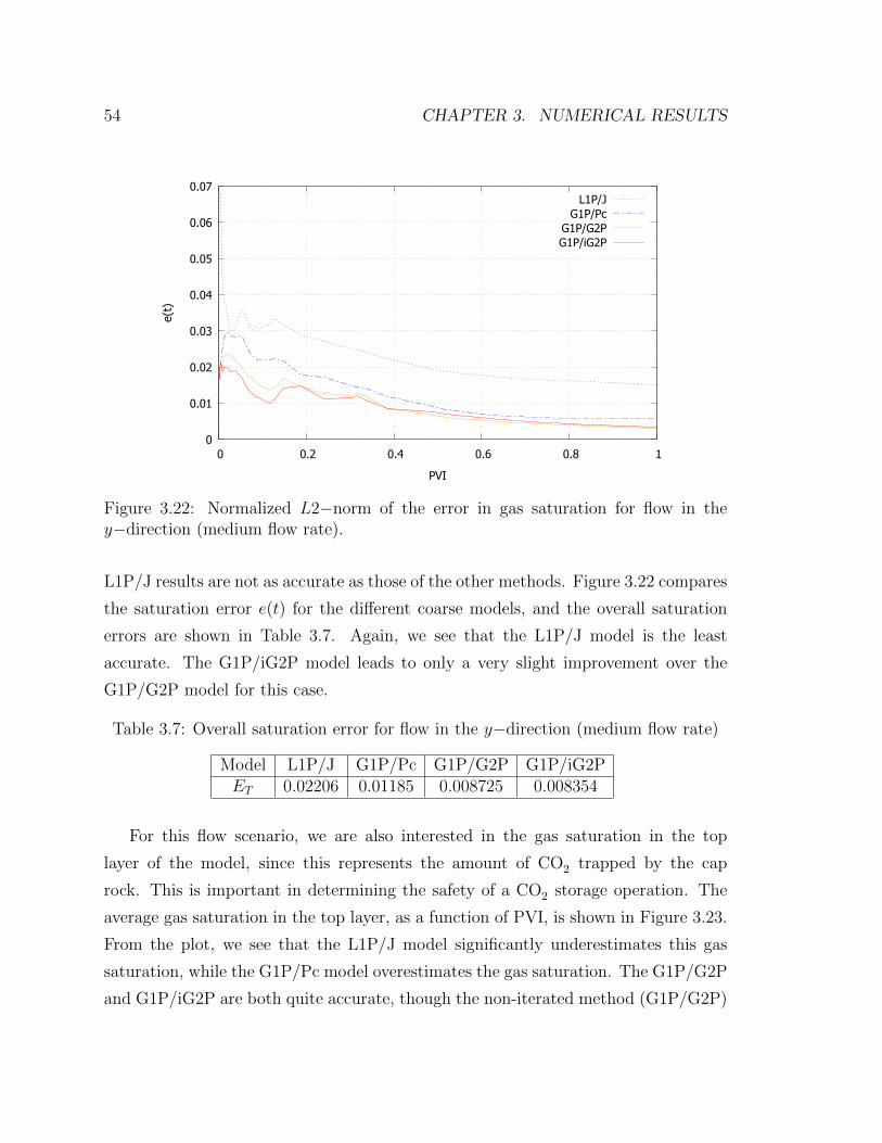
54 CHAPTER 3. NUMERICAL RESULTS
0
0.01
0.02
0.03
0.04
0.05
0.06
0.07
0 0.2 0.4 0.6 0.8 1
e(t)
PVI
L1P/JG1P/Pc
G1P/G2PG1P/iG2P
Figure 3.22: Normalized L2−norm of the error in gas saturation for flow in they−direction (medium flow rate).
L1P/J results are not as accurate as those of the other methods. Figure 3.22 compares
the saturation error e(t) for the different coarse models, and the overall saturation
errors are shown in Table 3.7. Again, we see that the L1P/J model is the least
accurate. The G1P/iG2P model leads to only a very slight improvement over the
G1P/G2P model for this case.
Table 3.7: Overall saturation error for flow in the y−direction (medium flow rate)
Model L1P/J G1P/Pc G1P/G2P G1P/iG2PET 0.02206 0.01185 0.008725 0.008354
For this flow scenario, we are also interested in the gas saturation in the top
layer of the model, since this represents the amount of CO2 trapped by the cap
rock. This is important in determining the safety of a CO2 storage operation. The
average gas saturation in the top layer, as a function of PVI, is shown in Figure 3.23.
From the plot, we see that the L1P/J model significantly underestimates this gas
saturation, while the G1P/Pc model overestimates the gas saturation. The G1P/G2P
and G1P/iG2P are both quite accurate, though the non-iterated method (G1P/G2P)
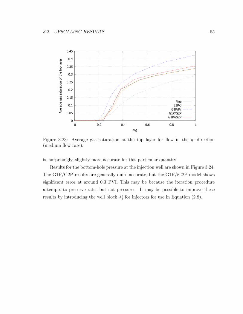
3.2. UPSCALING RESULTS 55
0
0.05
0.1
0.15
0.2
0.25
0.3
0.35
0.4
0.45
0 0.2 0.4 0.6 0.8 1
Aver
age
gas
satu
ratio
n of
the
top
laye
r
PVI
FineL1P/J
G1P/PcG1P/G2PG1P/iG2P
Figure 3.23: Average gas saturation at the top layer for flow in the y−direction(medium flow rate).
is, surprisingly, slightly more accurate for this particular quantity.
Results for the bottom-hole pressure at the injection well are shown in Figure 3.24.
The G1P/G2P results are generally quite accurate, but the G1P/iG2P model shows
significant error at around 0.3 PVI. This may be because the iteration procedure
attempts to preserve rates but not pressures. It may be possible to improve these
results by introducing the well block λ∗j for injectors for use in Equation (2.8).
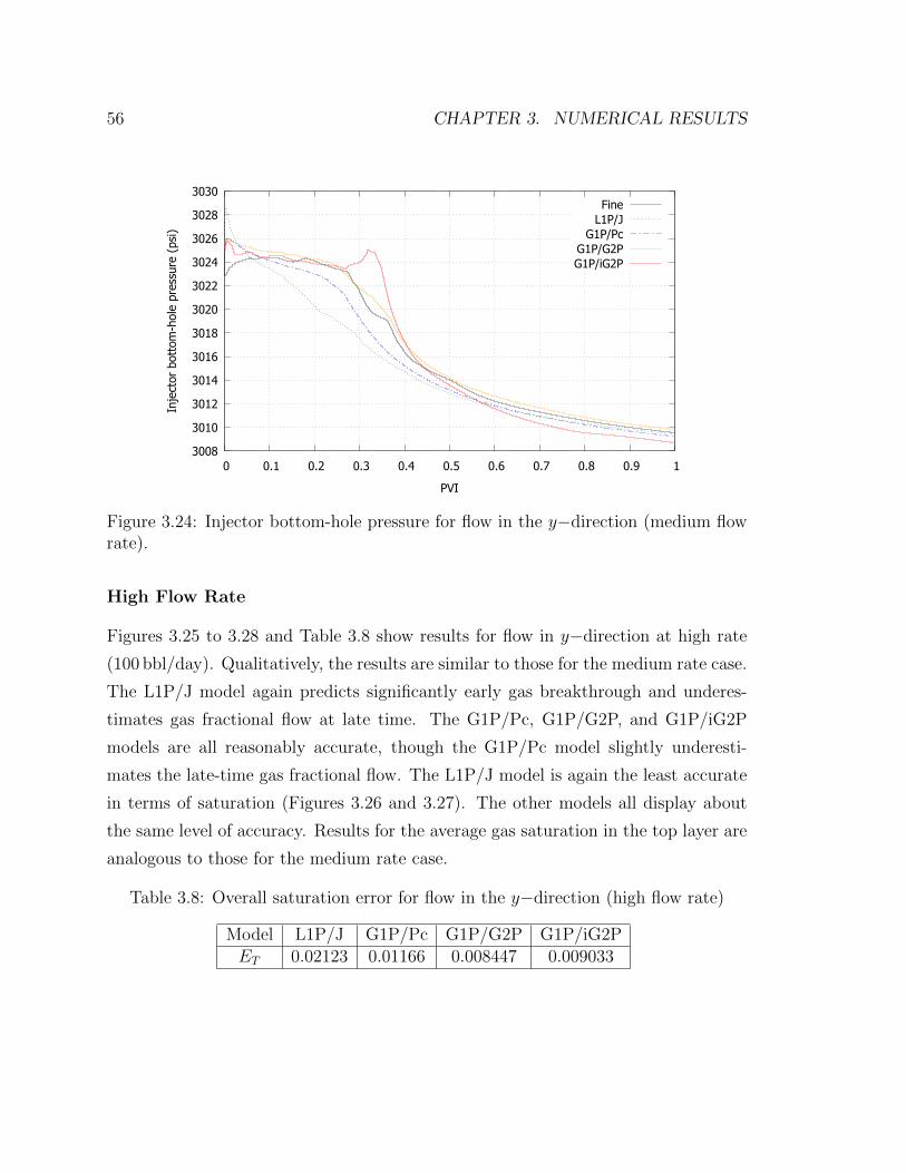
56 CHAPTER 3. NUMERICAL RESULTS
3008
3010
3012
3014
3016
3018
3020
3022
3024
3026
3028
3030
0 0.1 0.2 0.3 0.4 0.5 0.6 0.7 0.8 0.9 1
Inje
ctor
bot
tom
-hol
e pr
essu
re (
psi)
PVI
FineL1P/J
G1P/PcG1P/G2PG1P/iG2P
Figure 3.24: Injector bottom-hole pressure for flow in the y−direction (medium flowrate).
High Flow Rate
Figures 3.25 to 3.28 and Table 3.8 show results for flow in y−direction at high rate
(100 bbl/day). Qualitatively, the results are similar to those for the medium rate case.
The L1P/J model again predicts significantly early gas breakthrough and underes-
timates gas fractional flow at late time. The G1P/Pc, G1P/G2P, and G1P/iG2P
models are all reasonably accurate, though the G1P/Pc model slightly underesti-
mates the late-time gas fractional flow. The L1P/J model is again the least accurate
in terms of saturation (Figures 3.26 and 3.27). The other models all display about
the same level of accuracy. Results for the average gas saturation in the top layer are
analogous to those for the medium rate case.
Table 3.8: Overall saturation error for flow in the y−direction (high flow rate)
Model L1P/J G1P/Pc G1P/G2P G1P/iG2PET 0.02123 0.01166 0.008447 0.009033

3.2. UPSCALING RESULTS 57
0
0.2
0.4
0.6
0.8
1
0 0.1 0.2 0.3 0.4 0.5 0.6 0.7 0.8 0.9 1
Gas
fra
ctio
nal f
low
at
the
prod
ucer
PVI
FineL1P/J
G1P/PcG1P/G2PG1P/iG2P
Figure 3.25: Gas fractional flow at the producer for flow in the y−direction (high flowrate).
(a) Fine scale (b) Average fine scale
(c) Local k∗ with J−function (L1P/J) (d) Global T ∗ with CL P ∗c (G1P/Pc)
(e) Global T ∗ with CL P ∗c and global
λ∗j , no iteration (G1P/G2P)(f) Global T ∗ with CL P ∗
c and globalλ∗j , after iteration (G1P/iG2P)
Figure 3.26: Saturation map (Sg) at 0.425 PVI for flow in the y−direction (high flowrate).
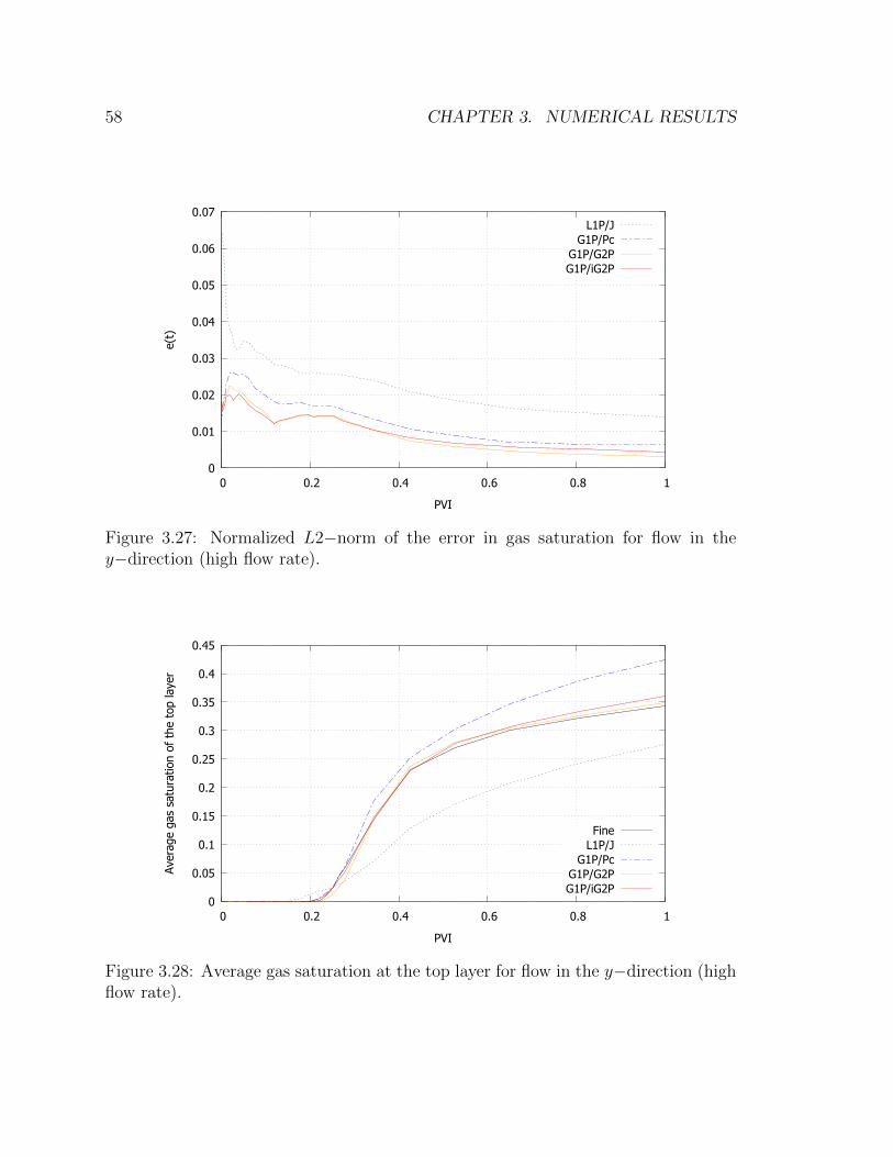
58 CHAPTER 3. NUMERICAL RESULTS
0
0.01
0.02
0.03
0.04
0.05
0.06
0.07
0 0.2 0.4 0.6 0.8 1
e(t)
PVI
L1P/JG1P/Pc
G1P/G2PG1P/iG2P
Figure 3.27: Normalized L2−norm of the error in gas saturation for flow in they−direction (high flow rate).
0
0.05
0.1
0.15
0.2
0.25
0.3
0.35
0.4
0.45
0 0.2 0.4 0.6 0.8 1
Aver
age
gas
satu
ratio
n of
the
top
laye
r
PVI
FineL1P/J
G1P/PcG1P/G2PG1P/iG2P
Figure 3.28: Average gas saturation at the top layer for flow in the y−direction (highflow rate).
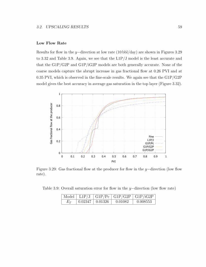
3.2. UPSCALING RESULTS 59
Low Flow Rate
Results for flow in the y−direction at low rate (10 bbl/day) are shown in Figures 3.29
to 3.32 and Table 3.9. Again, we see that the L1P/J model is the least accurate and
that the G1P/G2P and G1P/iG2P models are both generally accurate. None of the
coarse models capture the abrupt increase in gas fractional flow at 0.26 PVI and at
0.35 PVI, which is observed in the fine-scale results. We again see that the G1P/G2P
model gives the best accuracy in average gas saturation in the top layer (Figure 3.32).
0
0.2
0.4
0.6
0.8
1
0 0.1 0.2 0.3 0.4 0.5 0.6 0.7 0.8 0.9 1
Gas
fra
ctio
nal f
low
at
the
prod
ucer
PVI
FineL1P/J
G1P/PcG1P/G2PG1P/iG2P
Figure 3.29: Gas fractional flow at the producer for flow in the y−direction (low flowrate).
Table 3.9: Overall saturation error for flow in the y−direction (low flow rate)
Model L1P/J G1P/Pc G1P/G2P G1P/iG2PET 0.02347 0.01326 0.01082 0.008553
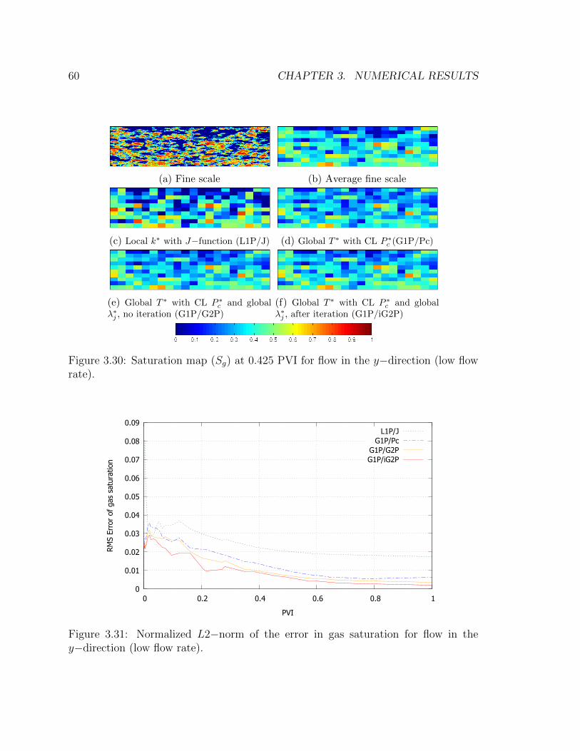
60 CHAPTER 3. NUMERICAL RESULTS
(a) Fine scale (b) Average fine scale
(c) Local k∗ with J−function (L1P/J) (d) Global T ∗ with CL P ∗c (G1P/Pc)
(e) Global T ∗ with CL P ∗c and global
λ∗j , no iteration (G1P/G2P)(f) Global T ∗ with CL P ∗
c and globalλ∗j , after iteration (G1P/iG2P)
Figure 3.30: Saturation map (Sg) at 0.425 PVI for flow in the y−direction (low flowrate).
0
0.01
0.02
0.03
0.04
0.05
0.06
0.07
0.08
0.09
0 0.2 0.4 0.6 0.8 1
RM
S Er
ror
of g
as s
atur
atio
n
PVI
L1P/JG1P/Pc
G1P/G2PG1P/iG2P
Figure 3.31: Normalized L2−norm of the error in gas saturation for flow in they−direction (low flow rate).
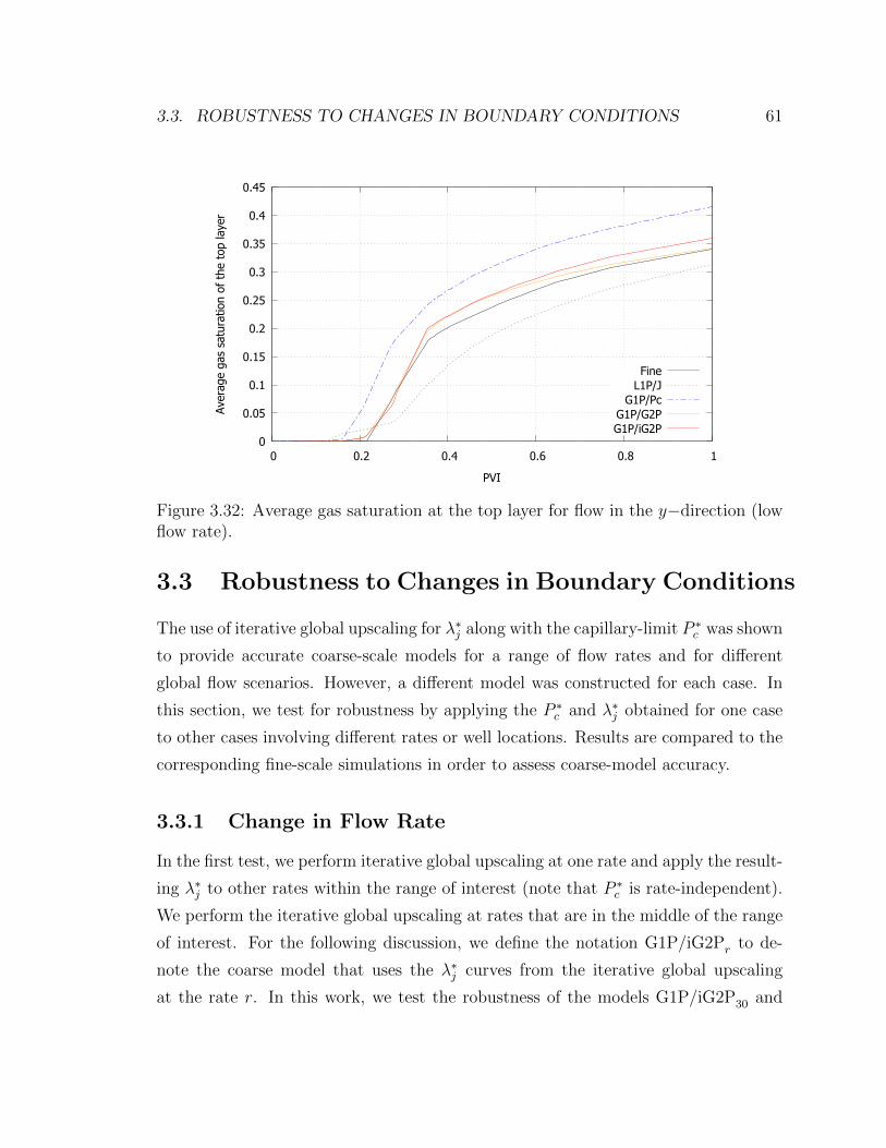
3.3. ROBUSTNESS TO CHANGES IN BOUNDARY CONDITIONS 61
0
0.05
0.1
0.15
0.2
0.25
0.3
0.35
0.4
0.45
0 0.2 0.4 0.6 0.8 1
Aver
age
gas
satu
ratio
n of
the
top
laye
r
PVI
FineL1P/J
G1P/PcG1P/G2PG1P/iG2P
Figure 3.32: Average gas saturation at the top layer for flow in the y−direction (lowflow rate).
3.3 Robustness to Changes in Boundary Conditions
The use of iterative global upscaling for λ∗j along with the capillary-limit P ∗c was shown
to provide accurate coarse-scale models for a range of flow rates and for different
global flow scenarios. However, a different model was constructed for each case. In
this section, we test for robustness by applying the P ∗c and λ∗j obtained for one case
to other cases involving different rates or well locations. Results are compared to the
corresponding fine-scale simulations in order to assess coarse-model accuracy.
3.3.1 Change in Flow Rate
In the first test, we perform iterative global upscaling at one rate and apply the result-
ing λ∗j to other rates within the range of interest (note that P ∗c is rate-independent).
We perform the iterative global upscaling at rates that are in the middle of the range
of interest. For the following discussion, we define the notation G1P/iG2Pr to de-
note the coarse model that uses the λ∗j curves from the iterative global upscaling
at the rate r. In this work, we test the robustness of the models G1P/iG2P30 and
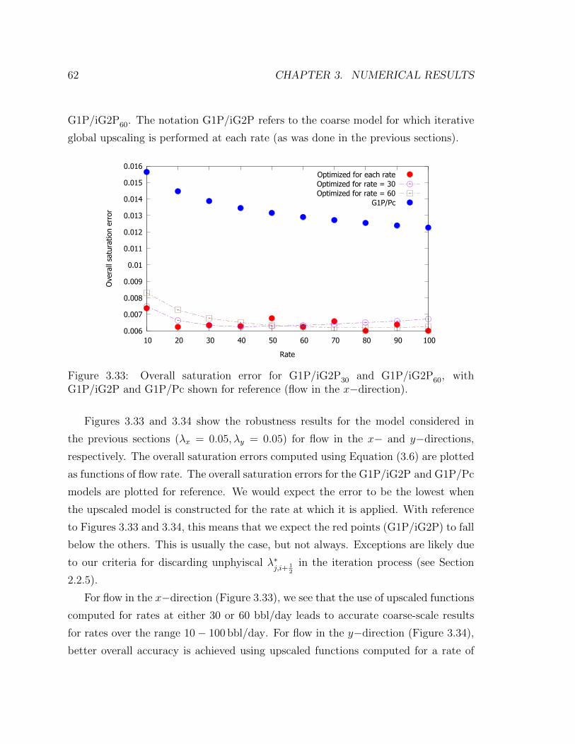
62 CHAPTER 3. NUMERICAL RESULTS
G1P/iG2P60. The notation G1P/iG2P refers to the coarse model for which iterative
global upscaling is performed at each rate (as was done in the previous sections).
0.006
0.007
0.008
0.009
0.01
0.011
0.012
0.013
0.014
0.015
0.016
10 20 30 40 50 60 70 80 90 100
Ove
rall
satu
ratio
n er
ror
Rate
Optimized for each rateOptimized for rate = 30Optimized for rate = 60
G1P/Pc
Figure 3.33: Overall saturation error for G1P/iG2P30 and G1P/iG2P60, withG1P/iG2P and G1P/Pc shown for reference (flow in the x−direction).
Figures 3.33 and 3.34 show the robustness results for the model considered in
the previous sections (λx = 0.05, λy = 0.05) for flow in the x− and y−directions,
respectively. The overall saturation errors computed using Equation (3.6) are plotted
as functions of flow rate. The overall saturation errors for the G1P/iG2P and G1P/Pc
models are plotted for reference. We would expect the error to be the lowest when
the upscaled model is constructed for the rate at which it is applied. With reference
to Figures 3.33 and 3.34, this means that we expect the red points (G1P/iG2P) to fall
below the others. This is usually the case, but not always. Exceptions are likely due
to our criteria for discarding unphyiscal λ∗j,i+ 1
2
in the iteration process (see Section
2.2.5).
For flow in the x−direction (Figure 3.33), we see that the use of upscaled functions
computed for rates at either 30 or 60 bbl/day leads to accurate coarse-scale results
for rates over the range 10− 100 bbl/day. For flow in the y−direction (Figure 3.34),
better overall accuracy is achieved using upscaled functions computed for a rate of
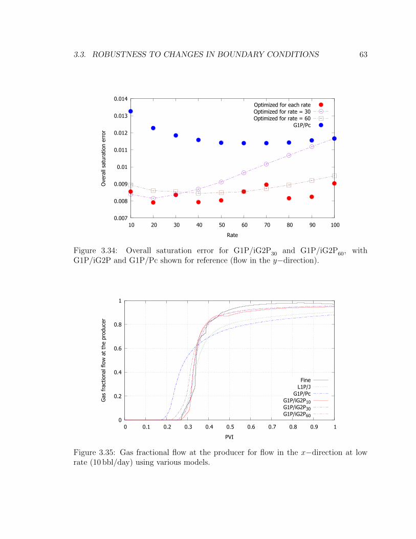
3.3. ROBUSTNESS TO CHANGES IN BOUNDARY CONDITIONS 63
0.007
0.008
0.009
0.01
0.011
0.012
0.013
0.014
10 20 30 40 50 60 70 80 90 100
Ove
rall
satu
ratio
n er
ror
Rate
Optimized for each rateOptimized for rate = 30Optimized for rate = 60
G1P/Pc
Figure 3.34: Overall saturation error for G1P/iG2P30 and G1P/iG2P60, withG1P/iG2P and G1P/Pc shown for reference (flow in the y−direction).
0
0.2
0.4
0.6
0.8
1
0 0.1 0.2 0.3 0.4 0.5 0.6 0.7 0.8 0.9 1
Gas
fra
ctio
nal f
low
at
the
prod
ucer
PVI
FineL1P/J
G1P/PcG1P/iG2P10G1P/iG2P30G1P/iG2P60
Figure 3.35: Gas fractional flow at the producer for flow in the x−direction at lowrate (10 bbl/day) using various models.
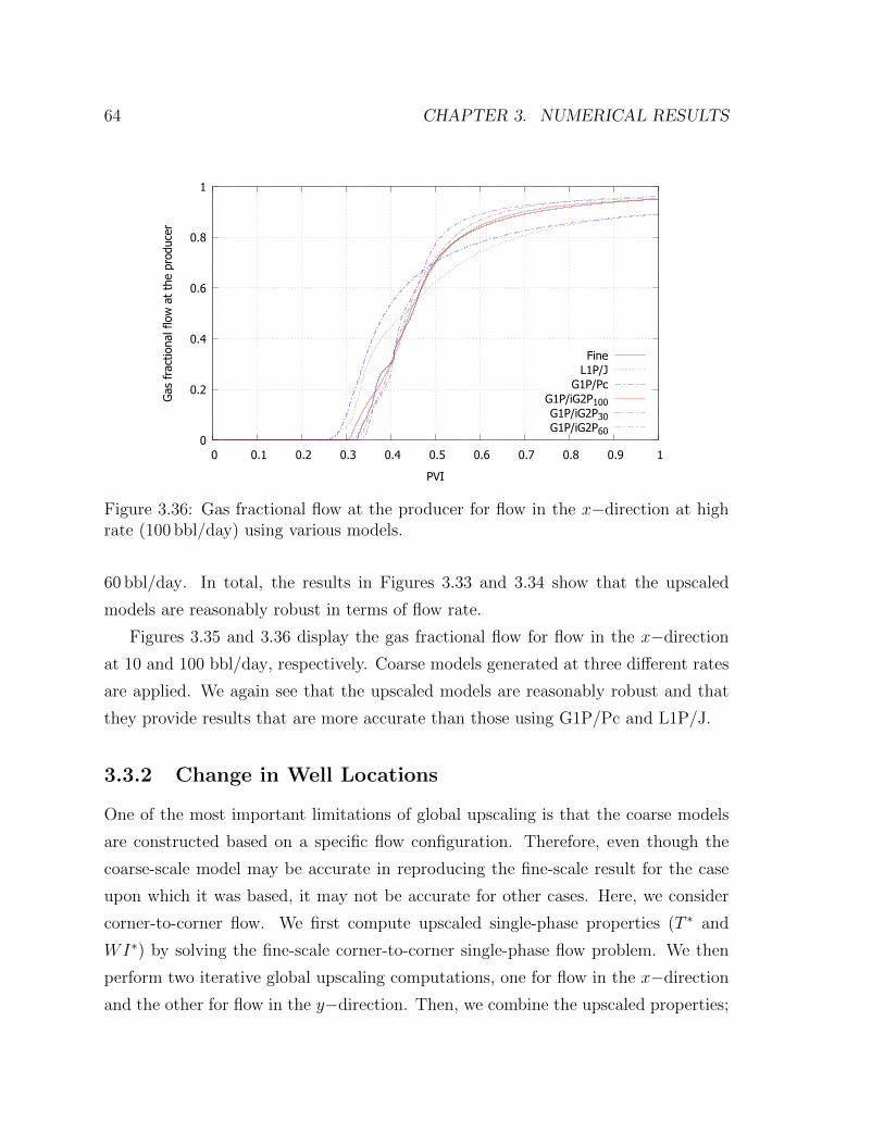
64 CHAPTER 3. NUMERICAL RESULTS
0
0.2
0.4
0.6
0.8
1
0 0.1 0.2 0.3 0.4 0.5 0.6 0.7 0.8 0.9 1
Gas
fra
ctio
nal f
low
at
the
prod
ucer
PVI
FineL1P/J
G1P/PcG1P/iG2P100G1P/iG2P30G1P/iG2P60
Figure 3.36: Gas fractional flow at the producer for flow in the x−direction at highrate (100 bbl/day) using various models.
60 bbl/day. In total, the results in Figures 3.33 and 3.34 show that the upscaled
models are reasonably robust in terms of flow rate.
Figures 3.35 and 3.36 display the gas fractional flow for flow in the x−direction
at 10 and 100 bbl/day, respectively. Coarse models generated at three different rates
are applied. We again see that the upscaled models are reasonably robust and that
they provide results that are more accurate than those using G1P/Pc and L1P/J.
3.3.2 Change in Well Locations
One of the most important limitations of global upscaling is that the coarse models
are constructed based on a specific flow configuration. Therefore, even though the
coarse-scale model may be accurate in reproducing the fine-scale result for the case
upon which it was based, it may not be accurate for other cases. Here, we consider
corner-to-corner flow. We first compute upscaled single-phase properties (T ∗ and
WI∗) by solving the fine-scale corner-to-corner single-phase flow problem. We then
perform two iterative global upscaling computations, one for flow in the x−direction
and the other for flow in the y−direction. Then, we combine the upscaled properties;
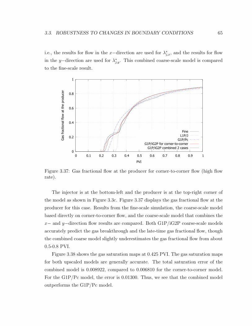
3.3. ROBUSTNESS TO CHANGES IN BOUNDARY CONDITIONS 65
i.e., the results for flow in the x−direction are used for λ∗j,x, and the results for flow
in the y−direction are used for λ∗j,y. This combined coarse-scale model is compared
to the fine-scale result.
0
0.2
0.4
0.6
0.8
1
0 0.1 0.2 0.3 0.4 0.5 0.6 0.7 0.8 0.9 1
Gas
fra
ctio
nal f
low
at
the
prod
ucer
PVI
FineL1P/J
G1P/PcG1P/iG2P for corner-to-corner
G1P/iG2P combined 2 cases
Figure 3.37: Gas fractional flow at the producer for corner-to-corner flow (high flowrate).
The injector is at the bottom-left and the producer is at the top-right corner of
the model as shown in Figure 3.3c. Figure 3.37 displays the gas fractional flow at the
producer for this case. Results from the fine-scale simulation, the coarse-scale model
based directly on corner-to-corner flow, and the coarse-scale model that combines the
x− and y−direction flow results are compared. Both G1P/iG2P coarse-scale models
accurately predict the gas breakthrough and the late-time gas fractional flow, though
the combined coarse model slightly underestimates the gas fractional flow from about
0.5-0.8 PVI.
Figure 3.38 shows the gas saturation maps at 0.425 PVI. The gas saturation maps
for both upscaled models are generally accurate. The total saturation error of the
combined model is 0.008922, compared to 0.006810 for the corner-to-corner model.
For the G1P/Pc model, the error is 0.01300. Thus, we see that the combined model
outperforms the G1P/Pc model.

66 CHAPTER 3. NUMERICAL RESULTS
(a) Fine scale (b) Average fine scale
(c) Global upscaling for corner-to-corner flow (G1P/iG2P)
(d) Combining the results from x−and y−directions
Figure 3.38: Saturation map at 0.425 PVI for the corner-to-corner flow (high flowrate).

Chapter 4
Conclusions and Future Work
4.1 Conclusions
• In this work, we developed a new iterative global upscaling method that is
applicable for two-phase flow with significant capillary pressure heterogeneity
effects. Upscaled capillary pressure functions are computed either analytically,
using the steady-state capillary-limit assumption, or numerically from fine-scale
flow results. Upscaled phase mobility (or relative permeability) functions are
computed in all cases using global fine-scale two-phase flow simulations. Itera-
tion on the upscaled functions based on coarse-scale simulation results provides
improved coarse-model accuracy.
• Numerical results for Gaussian permeability fields over a range of CO2 injection
rates demonstrated that the iterative global upscaling method provides accu-
rate coarse-scale models. These models were shown to accurately capture gas
breakthrough time, gas fractional flow and saturation distribution relative to
results from the corresponding fine-scale models. Coarse models generated us-
ing the new iterative global upscaling scheme were shown to be considerably
more accurate than coarse-scale models constructed using simpler approaches.
• The coarse-scale models with numerically computed P ∗c were shown to be slightly
more accurate than models with capillary-limit P ∗c . However, computation of
67
68 CHAPTER 4. CONCLUSIONS AND FUTURE WORK
P ∗c from the capillary-limit assumption is simpler and cleaner, as the results
do not depend on the specific flow conditions. We therefore recommend us-
ing capillary-limit P ∗c along with the iterative scheme for the upscaled mobility
functions.
• We tested the robustness of the coarse-scale models generated using iterative
global upscaling by running the upscaled models under different flow conditions.
The coarse-models were shown to be reasonably robust; i.e., they provided
coarse-scale results of sufficient accuracy for cases involving different flow rates
or large-scale flow configuration.
4.2 Future Work
• In this work, we only considered the flow of immiscible fluids in the horizontal
(x−y) plane, so gravity effects were not included. It will be useful to incorporate
these effects in future work, and to consider three-dimensional systems. The
dissolution of CO2 in water was also neglected, and these effects should be
included in the models and in the upscaling computations if necessary. Relative
permeability hysteresis effects should also be considered. When all of these
effects are incorporated, our coarse-scale models should be applicable for the
simulation of realistic carbon storage operations.
• We have shown that an upscaling procedure based on fine-scale global simula-
tions can provide an accurate coarse-scale model that is reasonably robust over
a range of CO2 injection rates. However, fine-scale global simulation is com-
putationally expensive, and it would be beneficial to avoid these computations.
Along these lines, extended-local or quasi-global (e.g., adaptive local-global or
ALG) upscaling approaches should be considered. Such an ALG procedure
would extend the work of Chen and Li (2009), who implemented ALG upscal-
ing for two-phase viscous-dominated flows.
• Additional robustness tests should be performed. A range of well locations
should be considered.
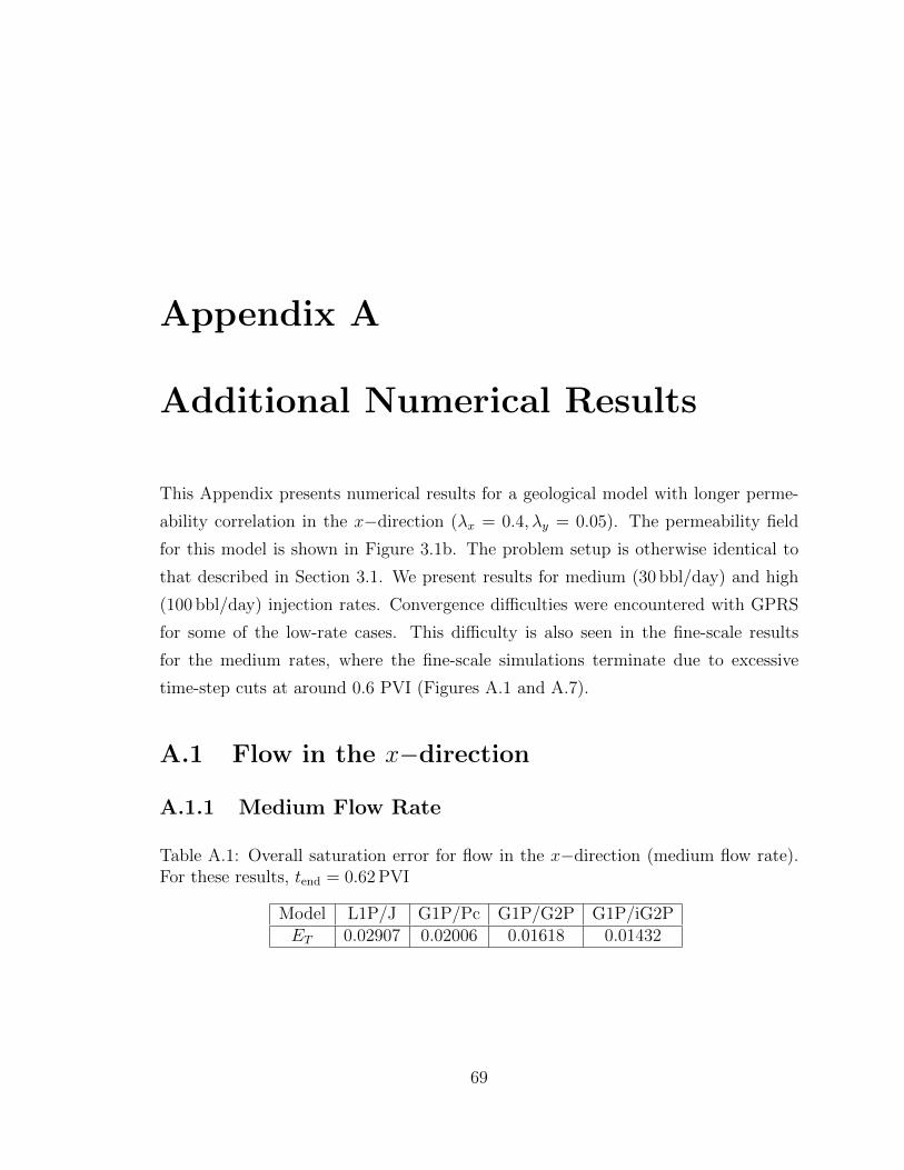
Appendix A
Additional Numerical Results
This Appendix presents numerical results for a geological model with longer perme-
ability correlation in the x−direction (λx = 0.4, λy = 0.05). The permeability field
for this model is shown in Figure 3.1b. The problem setup is otherwise identical to
that described in Section 3.1. We present results for medium (30 bbl/day) and high
(100 bbl/day) injection rates. Convergence difficulties were encountered with GPRS
for some of the low-rate cases. This difficulty is also seen in the fine-scale results
for the medium rates, where the fine-scale simulations terminate due to excessive
time-step cuts at around 0.6 PVI (Figures A.1 and A.7).
A.1 Flow in the x−direction
A.1.1 Medium Flow Rate
Table A.1: Overall saturation error for flow in the x−direction (medium flow rate).For these results, tend = 0.62 PVI
Model L1P/J G1P/Pc G1P/G2P G1P/iG2PET 0.02907 0.02006 0.01618 0.01432
69

70 APPENDIX A. ADDITIONAL NUMERICAL RESULTS
0
0.2
0.4
0.6
0.8
1
0 0.1 0.2 0.3 0.4 0.5 0.6 0.7 0.8 0.9 1
Gas
fra
ctio
nal f
low
at
the
prod
ucer
PVI
FineL1P/J
G1P/PcG1P/G2PG1P/iG2P
Figure A.1: Gas fractional flow at the producer for flow in the x−direction (mediumflow rate).
(a) Fine scale (b) Average fine scale
(c) Local k∗ with J−function (L1P/J) (d) Global T ∗ with CL P ∗c (G1P/Pc)
(e) Global T ∗ with CL P ∗c and global
λ∗j , no iteration (G1P/G2P)(f) Global T ∗ with CL P ∗
c and globalλ∗j , after iteration (G1P/iG2P)
Figure A.2: Saturation map (Sg) at 0.425 PVI for flow in the x−direction (mediumflow rate).
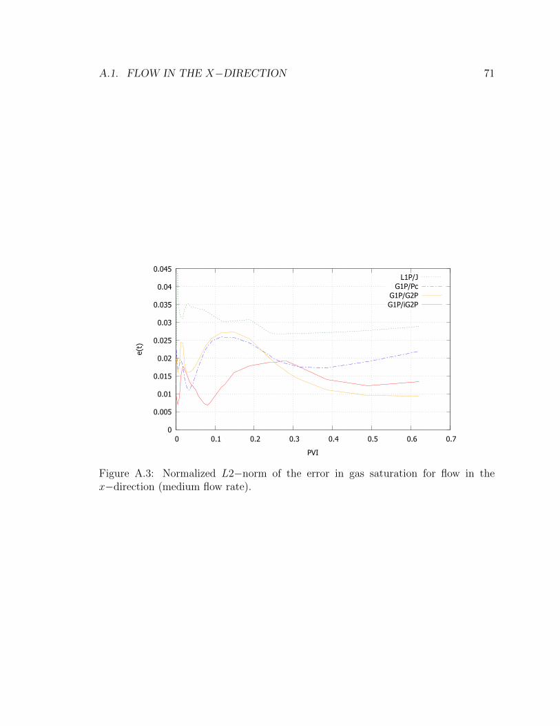
A.1. FLOW IN THE X−DIRECTION 71
0
0.005
0.01
0.015
0.02
0.025
0.03
0.035
0.04
0.045
0 0.1 0.2 0.3 0.4 0.5 0.6 0.7
e(t)
PVI
L1P/JG1P/Pc
G1P/G2PG1P/iG2P
Figure A.3: Normalized L2−norm of the error in gas saturation for flow in thex−direction (medium flow rate).
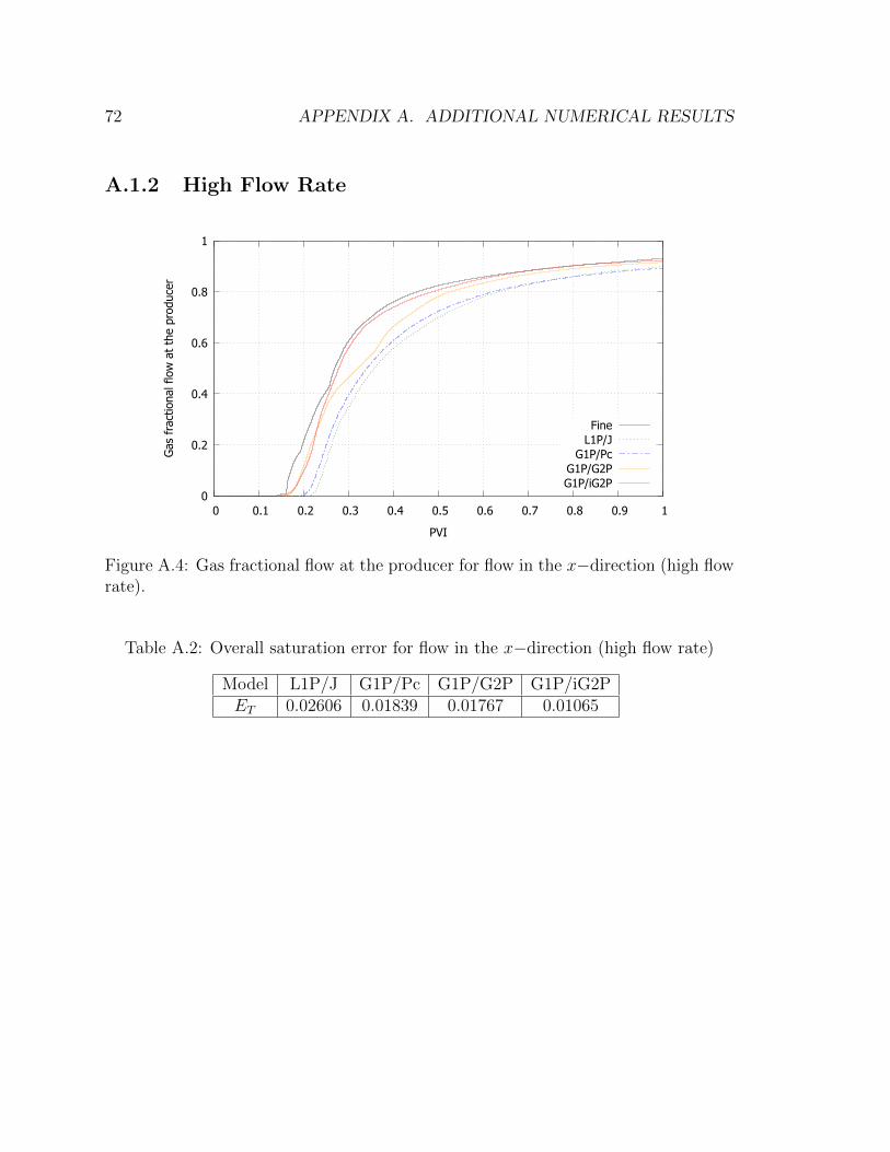
72 APPENDIX A. ADDITIONAL NUMERICAL RESULTS
A.1.2 High Flow Rate
0
0.2
0.4
0.6
0.8
1
0 0.1 0.2 0.3 0.4 0.5 0.6 0.7 0.8 0.9 1
Gas
fra
ctio
nal f
low
at
the
prod
ucer
PVI
FineL1P/J
G1P/PcG1P/G2PG1P/iG2P
Figure A.4: Gas fractional flow at the producer for flow in the x−direction (high flowrate).
Table A.2: Overall saturation error for flow in the x−direction (high flow rate)
Model L1P/J G1P/Pc G1P/G2P G1P/iG2PET 0.02606 0.01839 0.01767 0.01065
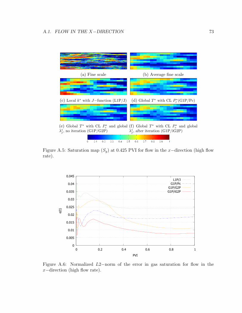
A.1. FLOW IN THE X−DIRECTION 73
(a) Fine scale (b) Average fine scale
(c) Local k∗ with J−function (L1P/J) (d) Global T ∗ with CL P ∗c (G1P/Pc)
(e) Global T ∗ with CL P ∗c and global
λ∗j , no iteration (G1P/G2P)(f) Global T ∗ with CL P ∗
c and globalλ∗j , after iteration (G1P/iG2P)
Figure A.5: Saturation map (Sg) at 0.425 PVI for flow in the x−direction (high flowrate).
0
0.005
0.01
0.015
0.02
0.025
0.03
0.035
0.04
0.045
0 0.2 0.4 0.6 0.8 1
e(t)
PVI
L1P/JG1P/Pc
G1P/G2PG1P/iG2P
Figure A.6: Normalized L2−norm of the error in gas saturation for flow in thex−direction (high flow rate).
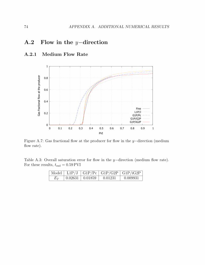
74 APPENDIX A. ADDITIONAL NUMERICAL RESULTS
A.2 Flow in the y−direction
A.2.1 Medium Flow Rate
0
0.2
0.4
0.6
0.8
1
0 0.1 0.2 0.3 0.4 0.5 0.6 0.7 0.8 0.9 1
Gas
fra
ctio
nal f
low
at
the
prod
ucer
PVI
FineL1P/J
G1P/PcG1P/G2PG1P/iG2P
Figure A.7: Gas fractional flow at the producer for flow in the y−direction (mediumflow rate).
Table A.3: Overall saturation error for flow in the y−direction (medium flow rate).For these results, tend = 0.59 PVI
Model L1P/J G1P/Pc G1P/G2P G1P/iG2PET 0.02631 0.01859 0.01231 0.009931
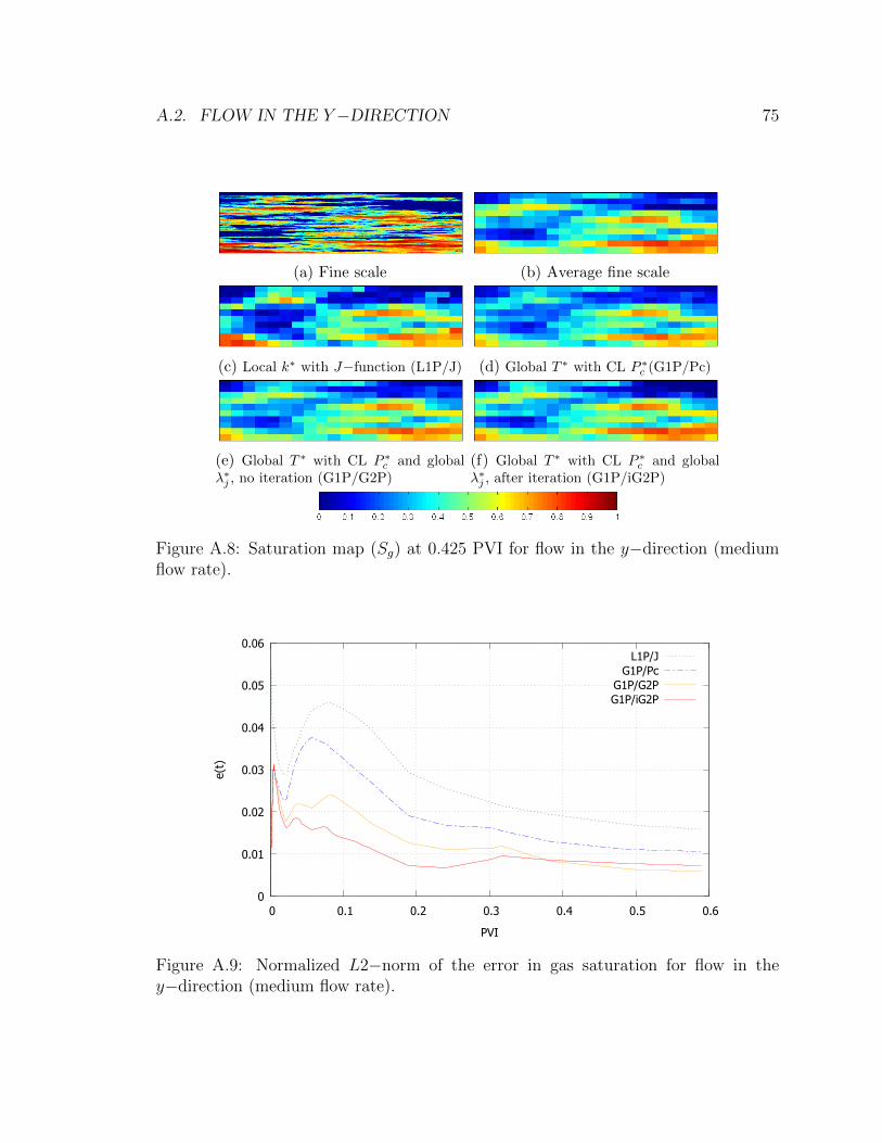
A.2. FLOW IN THE Y−DIRECTION 75
(a) Fine scale (b) Average fine scale
(c) Local k∗ with J−function (L1P/J) (d) Global T ∗ with CL P ∗c (G1P/Pc)
(e) Global T ∗ with CL P ∗c and global
λ∗j , no iteration (G1P/G2P)(f) Global T ∗ with CL P ∗
c and globalλ∗j , after iteration (G1P/iG2P)
Figure A.8: Saturation map (Sg) at 0.425 PVI for flow in the y−direction (mediumflow rate).
0
0.01
0.02
0.03
0.04
0.05
0.06
0 0.1 0.2 0.3 0.4 0.5 0.6
e(t)
PVI
L1P/JG1P/Pc
G1P/G2PG1P/iG2P
Figure A.9: Normalized L2−norm of the error in gas saturation for flow in they−direction (medium flow rate).
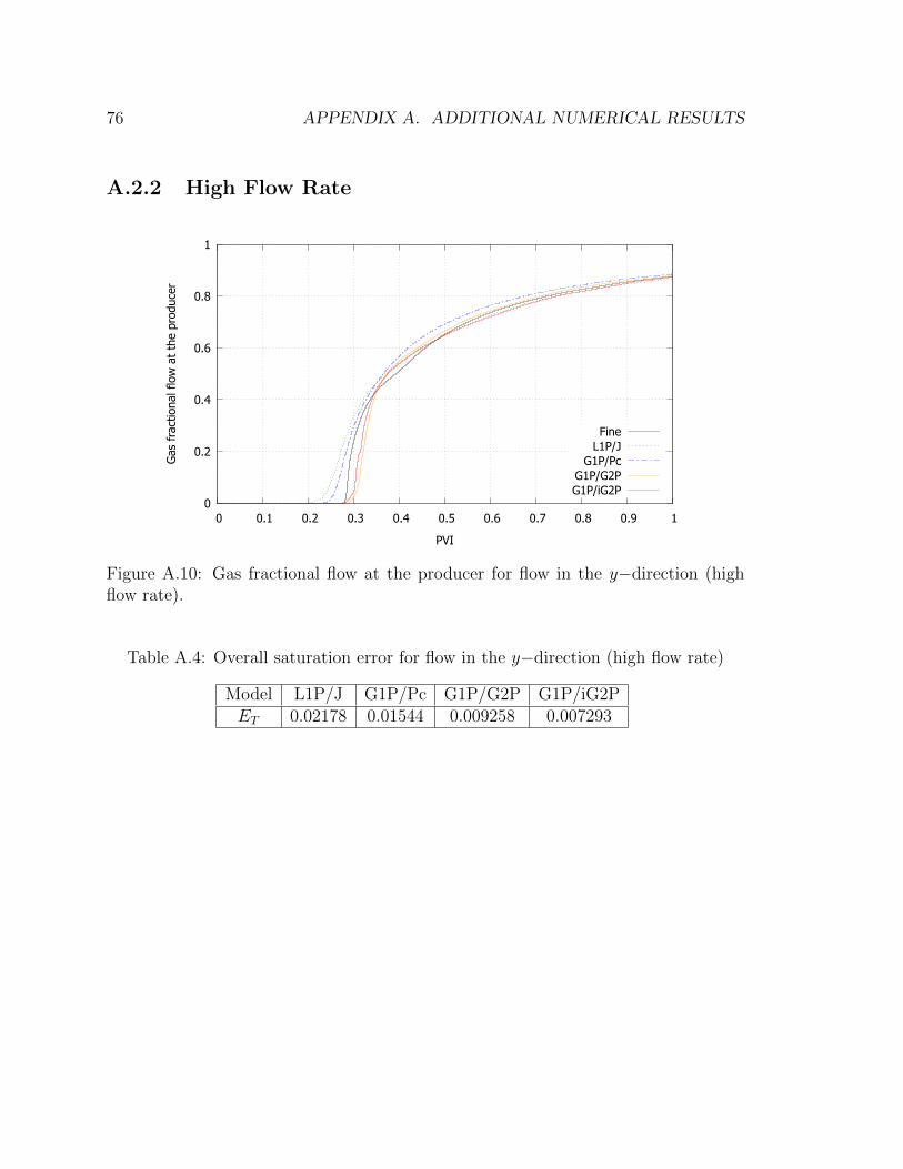
76 APPENDIX A. ADDITIONAL NUMERICAL RESULTS
A.2.2 High Flow Rate
0
0.2
0.4
0.6
0.8
1
0 0.1 0.2 0.3 0.4 0.5 0.6 0.7 0.8 0.9 1
Gas
fra
ctio
nal f
low
at
the
prod
ucer
PVI
FineL1P/J
G1P/PcG1P/G2PG1P/iG2P
Figure A.10: Gas fractional flow at the producer for flow in the y−direction (highflow rate).
Table A.4: Overall saturation error for flow in the y−direction (high flow rate)
Model L1P/J G1P/Pc G1P/G2P G1P/iG2PET 0.02178 0.01544 0.009258 0.007293
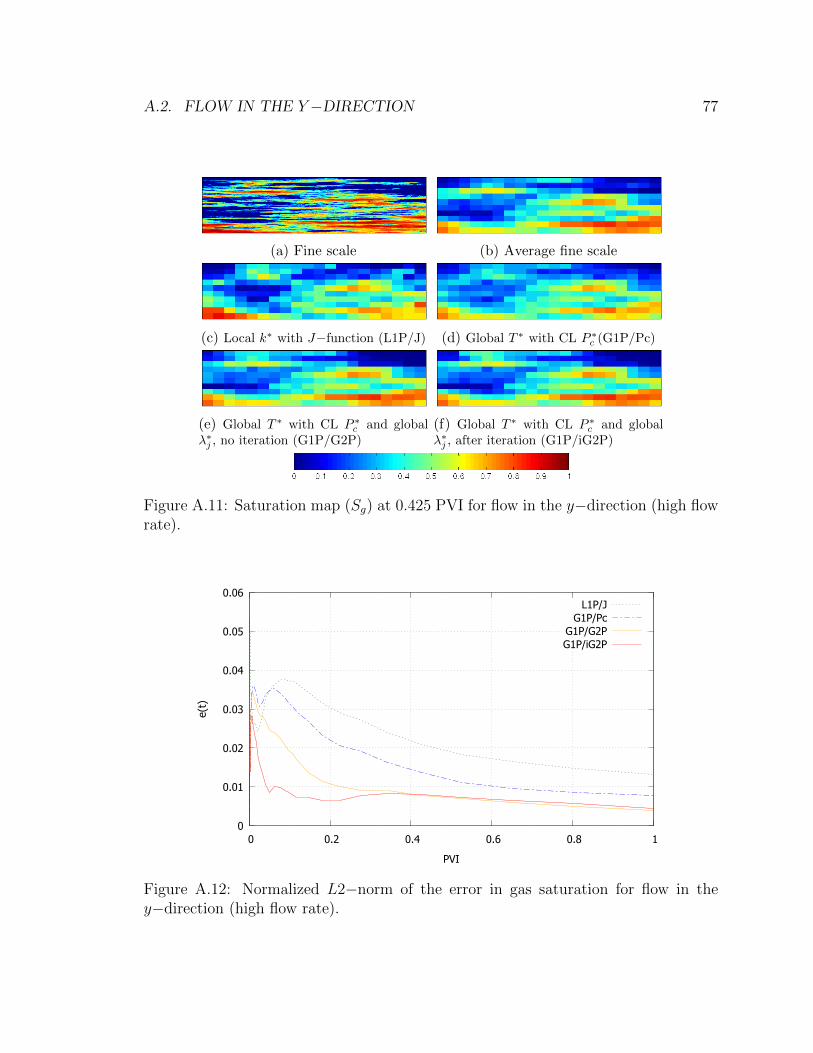
A.2. FLOW IN THE Y−DIRECTION 77
(a) Fine scale (b) Average fine scale
(c) Local k∗ with J−function (L1P/J) (d) Global T ∗ with CL P ∗c (G1P/Pc)
(e) Global T ∗ with CL P ∗c and global
λ∗j , no iteration (G1P/G2P)(f) Global T ∗ with CL P ∗
c and globalλ∗j , after iteration (G1P/iG2P)
Figure A.11: Saturation map (Sg) at 0.425 PVI for flow in the y−direction (high flowrate).
0
0.01
0.02
0.03
0.04
0.05
0.06
0 0.2 0.4 0.6 0.8 1
e(t)
PVI
L1P/JG1P/Pc
G1P/G2PG1P/iG2P
Figure A.12: Normalized L2−norm of the error in gas saturation for flow in they−direction (high flow rate).

78 APPENDIX A. ADDITIONAL NUMERICAL RESULTS

Nomenclature
Abbreviations
G1P/Pc global T ∗ with capillary-limit P ∗c and rock curves for krj
G1P/G2P global T ∗ with capillary-limit P ∗c and global k∗rj with no iteration
G1P/G2PPc global T ∗ with numerically computed P ∗c and global k∗rj with no iter-
ation
G1P/iG2P global T ∗ with capillary-limit P ∗c and iterated global k∗rj
G1P/iG2PPc global T ∗ with iterated global k∗rj and P ∗c
G1P/iG2Pr coarse-scale model generated from the iterative global upscaling with
a specified flow rate of r bbl/day
GPRS General Purpose Research Simulator
L1P/J local k∗ with J−function and rock curves for krj
PVI pore volume injected
Variables
Dx, Dy fine-scale block size in the x− and y−directions
e normalized L2−norm of differences between fine-scale and coarse-scale
saturations
ET overall saturation error
79
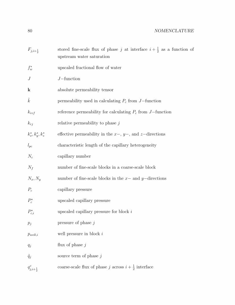
80 NOMENCLATURE
Fj,i+ 12
stored fine-scale flux of phase j at interface i+ 12
as a function of
upstream water saturation
f ∗w upscaled fractional flow of water
J J−function
k absolute permeability tensor
k permeability used in calculating Pc from J−function
kref reference permeability for calculating Pc from J−function
krj relative permeability to phase j
k∗x, k∗y, k
∗z effective permeability in the x−, y−, and z−directions
lpc characteristic length of the capillary heterogeneity
Nc capillary number
Nf number of fine-scale blocks in a coarse-scale block
Nx, Ny number of fine-scale blocks in the x− and y−directions
Pc capillary pressure
P ∗c upscaled capillary pressure
P ∗c,i upscaled capillary pressure for block i
pj pressure of phase j
pwell,i well pressure in block i
qj flux of phase j
qj source term of phase j
qcj,i+ 1
2
coarse-scale flux of phase j across i+ 12
interface
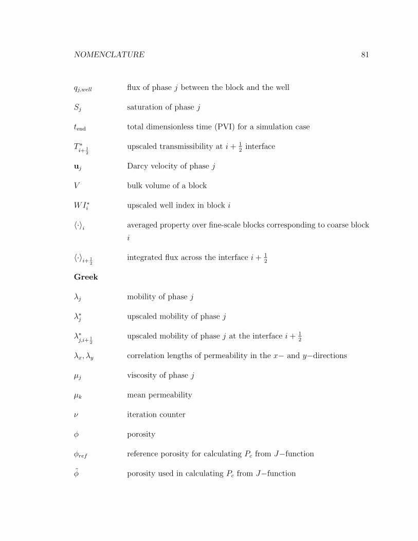
NOMENCLATURE 81
qj,well flux of phase j between the block and the well
Sj saturation of phase j
tend total dimensionless time (PVI) for a simulation case
T ∗i+ 1
2
upscaled transmissibility at i+ 12
interface
uj Darcy velocity of phase j
V bulk volume of a block
WI∗i upscaled well index in block i
〈·〉i averaged property over fine-scale blocks corresponding to coarse block
i
〈·〉i+ 12
integrated flux across the interface i+ 12
Greek
λj mobility of phase j
λ∗j upscaled mobility of phase j
λ∗j,i+ 1
2
upscaled mobility of phase j at the interface i+ 12
λx, λy correlation lengths of permeability in the x− and y−directions
µj viscosity of phase j
µk mean permeability
ν iteration counter
φ porosity
φref reference porosity for calculating Pc from J−function
φ porosity used in calculating Pc from J−function

82 NOMENCLATURE
σln k standard deviation of log permeability
Subscripts
g gas
j phase
w water
Superscripts
∗ upscaled quantity
c coarse-scale property
cap flux due to difference in capillary pressure
conv flux due to difference in gas pressure
f fine-scale property
Bibliography
H. Behzadi and V. Alvarado. Upscaling of upward CO2 migration in 2D system.
Advances in Water Resources, 46:46–54, 2012.
R. H. Brooks and A. T. Corey. Hydraulic properties of porous media. Hydrology
Papers, Colorado State University, 1964.
H. Cao. Deveopment of Techniques for General Purpose Simulators. PhD thesis,
Stanford University, 2002.
C. Chasset, J. Jarsjo, M. Erlstrom, V. Cvetkovic, and G. Destouni. Scenario simula-
tions of CO2 injection feasibility, plume migration and storage in a saline aquifer,
Scania, Sweden. International Journal of Greenhouse Gas Control, 5(5):1303–1318,
2011.
T. Chen, M. G. Gerritsen, J. V. Lambers, and L. J. Durlofsky. Global variable
compact multipoint methods for accurate upscaling with full-tensor effects. Com-
putational Geosciences, 14(1):65–81, 2010.
Y. Chen. Upscaling and Subgrid Modeling of Flow and Transport in Heterogeneous
Reservoirs. PhD thesis, Stanford University, 2005.
Y. Chen and Y. Li. Local-global two-phase upscaling of flow and transport in het-
erogeneous formations. Multiscale Modeling & Simulation, 8(1):125–153, 2009.
Y. Chen, L. J. Durlofsky, M. Gerritsen, and X.-H. Wen. A coupled local-global up-
scaling approach for simulating flow in highly heterogeneous formations. Advances
in Water Resources, 26(10):1041–1060, 2003.
83
84 BIBLIOGRAPHY
Y. Chen, B. T. Mallison, and L. J. Durlofsky. Nonlinear two-point flux approxima-
tion for modeling full-tensor effects in subsurface flow simulations. Computational
Geosciences, 12(3):317–335, 2008.
N. H. Darman and G. E. Pickup. The development of pseudo functions for gravity-
dominated immiscible gas displacements. In Proceedings of the SPE Reservoir
Simulation Symposium, Houston, TX, SPE 51941, 1999.
N. H. Darman, G. E. Pickup, and K. S. Sorbie. A comparison of two-phase dynamic
upscaling methods based on fluid potentials. Computational Geosciences, 6(1):
5–27, 2002.
C. V. Deutsch and A. G. Journel. GSLIB: Geostatistical Software Library and User’s
Guide. Oxford University Press, New York, 1992.
C. Doughty. Investigation of CO2 plume behavior for a large-scale pilot test of geologic
carbon storage in a saline formation. Transport in Porous Media, 82(1):49–76, 2010.
L. J. Durlofsky. Upscaling and gridding of fine scale geological models for flow sim-
ulation. In Proceedings of the 8th International Forum on Reservoir Simulation,
Stresa, Italy, 2005.
S. Ekrann and M. Dale. Averaging of relative permeability in heterogeneous reservoirs.
In Proceedings of the 3rd European Conference on the Mathematics of Oil Recovery,
Delft, The Netherlands, 1992.
S. Ghanbari, Y. Al-Zaabi, G. E. Pickup, E. Mackay, F. Gozalpour, and A. C. Todd.
Simulation of CO2 storage in saline aquifers. Chemical Engineering Research and
Design, 84(9):764–775, 2006.
W. S. Han, B. J. McPherson, P. C. Lichtner, and F. P. Wang. Evaluation of trapping
mechanisms in geologic CO2 sequestration: Case study of SACROC northern plat-
form, a 35-year CO2 injection site. American Journal of Science, 310(4):282–324,
2010.
BIBLIOGRAPHY 85
T. Hewett and R. Archer. Scale-averaged effective flow properties for coarse-grid
reservoir simulation. In Proceedings of the SPE Reservoir Simulation Symposium,
Dallas, TX, SPE 37988, 1997.
S. T. Ide, K. Jessen, and F. M. Orr Jr. Storage of CO2 in saline aquifers: Effects of
gravity, viscous, and capillary forces on amount and timing of trapping. Interna-
tional Journal of Greenhouse Gas Control, 1(4):481–491, 2007.
S. Krevor, R. Pini, B. Li, and S. M. Benson. Capillary heterogeneity trapping of CO2
in a sandstone rock at reservoir conditions. Geophysical Research Letters, 38(15),
2011.
A. Kumar, M. Noh, G. A. Pope, K. Sepehrnoori, S. Bryant, and L. W. Lake. Reservoir
simulation of CO2 storage in deep saline aquifers. In Proceedings of the SPE/DOE
Symposium on Improved Oil Recovery, Tulsa, OK, SPE 89343, 2004.
J. R. Kyte and D. W. Berry. New pseudo functions to control numerical dispersion.
SPE Journal, 15(4):269–276, 1975.
E. W. Lemmon, M. O. McLinden, and D. G. Friend. Thermophysical Properties of
Fluid Systems. 2005. URL http://webbook.nist.gov.
M. C. Leverett. Capillary behavior in porous solids. Transactions of the AIME, 1940.
B. Li, S. M. Benson, and H. A. Tchelepi. Modeling fine-scale capillary heterogeneity in
multiphase flow of CO2 and brine in sedimentary rocks. In Proceedings of the XIX
International Conference on Computational Methods in Water Resources, Urbana,
IL, 2012.
A. Lohne, G. Virnovsky, and L. J. Durlofsky. Two-stage upscaling of two-phase flow:
From core to simulation scale. SPE Journal, 11(3):304–316, 2006.
S. Mo and I. Akervoll. Modeling long-term CO2 storage in aquifer with a black-
oil reservoir simulator. In Proceedings of the SPE/EPA/DOE Exploration and
Production Environmental Conference, Galveston, TX, SPE 93951, 2005.
86 BIBLIOGRAPHY
E. Mouche, M. Hayek, and C. Mugler. Upscaling of CO2 vertical migration through a
periodic layered porous medium: The capillary-free and capillary-dominant cases.
Advances in Water Resources, 33(9):1164–1175, 2010.
A. Ng. CS229 lecture notes. University Lecture Notes, 2012. URL
http://cs229.stanford.edu/.
G. E. Pickup and K. S. Sorbie. Scaleup of two-phase flow in porous media using phase
permeability tensors. SPE Journal, 1(4):369–382, 1996.
E. Saadatpoor, S. L. Bryant, and K. Sepehrnoori. New trapping mechanism in carbon
sequestration. Transport in Porous Media, 82(1):3–17, 2010.
E. Saadatpoor, S. L. Bryant, and K. Sepehrnoori. Effect of upscaling heterogeneous
domain on CO2 trapping mechanisms. Energy Procedia, 4:5066–5073, 2011.
H. Stone. Rigorous black oil pseudo functions. In Proceedings of the SPE Reservoir
Simulation Symposium, Anaheim, CA, SPE 21207, 1991.
G. A. Virnovsky, H. A. Friis, and A. Lohne. A steady-state upscaling approach for
immiscible two-phase flow. Transport in Porous Media, 54(2):167–192, 2004.
T. C. Wallstrom, M. A. Christie, L. J. Durlofsky, and D. H. Sharp. Effective flux
boundary conditions for upscaling porous media equations. Transport in Porous
Media, 46(2-3):139–153, 2002.