USE OF A KALMAN FILTER TO IMPROVE REALTIME VIDEO STREAM IMAGEPROCESSING: AN EXAMPLE

PATRICK D. O’MALLEY

A HIGHEST HONORS REPORT PRESENTED TO THE COLLEGE OF ENGINEERING INPARTIAL FULFILLMENT OF THE REQUIREMENTS FOR THE DEGREE OF BACHELOR OF

SCIENCE IN COMPUTER ENGINEERING

Fall 2000

Acknowledgments

I would like to thank Dr. Michael Nechyba of the University of FloridaElectrical and Electrical Engineering department for the great help he gaveme in preparing this and in funding me so I can spend my time doingthings I like to do.

I would like to thank Dr. Arroyo, also of the UF ECE department forgiving me the opportunity of working in the Machine Intelligence Lab.

I would like to thank everyone else in the Machine Intelligence Lab forputting up with me for four long years.

And, of course, my parents without whom I would not be here today.

~ 1 ~

Table of Contents

List of Tables 3

List of Figures 3

Key to Abbreviations 4

Chapter One − Introduction 5

Purpose 5

Background 5

Current Algorithms 8

Chapter Two − Improved Bounding Box Algorithm 11

Summary 11

The Kalman Filter 11

Bounding Box Prediction 15

Effects of Misprediction 16

Chapter Three − Implementation 22

Chapter Four − Results 23

Bounding Box Size 23

Probability of Finding the Car Inside theImproved Bounding Box

23

Conclusion 24

References 26

Appendix A − MATLAB 27

Appendix B − Java Kalman Filter Implementation 30

~ 2 ~

List of Tables Page

Table 1: Kalman filter time update equations (predict) 11

Table 2: Kalman filter measurement update equations (correct) 11

Table 3: Comparison of Bounding Box Sizes 23

List of Figures Page

Figure 1: The track 6

Figure 2: Video stream processing setup 7

Figure 3: Bounding Boxes 10

Figure 4: The track coordinate system 13

Figure 5: Comparison of predicted versus measured S−coordinate values 17

Figure 6: Difference between predicted and measured S−coordinate values 18

Figure 7: Unfiltered and filtered velocity in the S direction 19

Figure 8: Unfiltered and filtered velocity in the T direction 20

Figure 9: Unfiltered and filtered car position in the T direction 21

Figure 10: Successful bounding box prediction 25

Figure 11: Successful bounding box prediction 25

~ 3 ~

Key to Symbols and Abbreviations

NTSC National Television Standards Committee: The signalstandard for video broadcast in the United States

FPS Frames Per Second

S−Video A standard NTSC signal transmission medium

~ 4 ~

CHAPTER 1

INTRODUCTION

Purpose

Real−time video stream image processing is extremely computationally

expensive. Due to the amount of information carried in a video data stream, only recently

have personal computers become fast enough to make this form of analysis feasible to

use when one is on a tight budget. For example, one second of video at 30 frames per

second (FPS) and a digital resolution of 640 pixels wide by 480 pixels high and a color

depth of 24 bits per pixel gives a total data throughput of 27.65 megabytes/second. To

work in real time, an algorithm must produce meaningful data based on each frame of

incoming, live video. The best−case−scenario − image analysis at 30 FPS − means that

the algorithms have around 33ms to produce data and this does not include time for the

image capture equipment or any other overhead produced by the computer or operating

system. Obviously, as computers become faster the problem will diminish but it is always

useful to develop ways to reduce the computational cost of a problem as long as it does

not interfere with the solution. One such way of speeding video stream analysis is

presented herein.

Background

Since the Fall 1999 semester, Dr. Michael Nechyba and others at the University

of Florida Machine Intelligence Lab have been working on a project involving image

analysis of video streams in realtime. More specifically, the project has recovered the

three dimensional location and orientation (also known as ’pose’) of an arbitrary number

of small cars circling on a ’slot−car’ track − a common toy purchased at a local toy store.

~ 5 ~

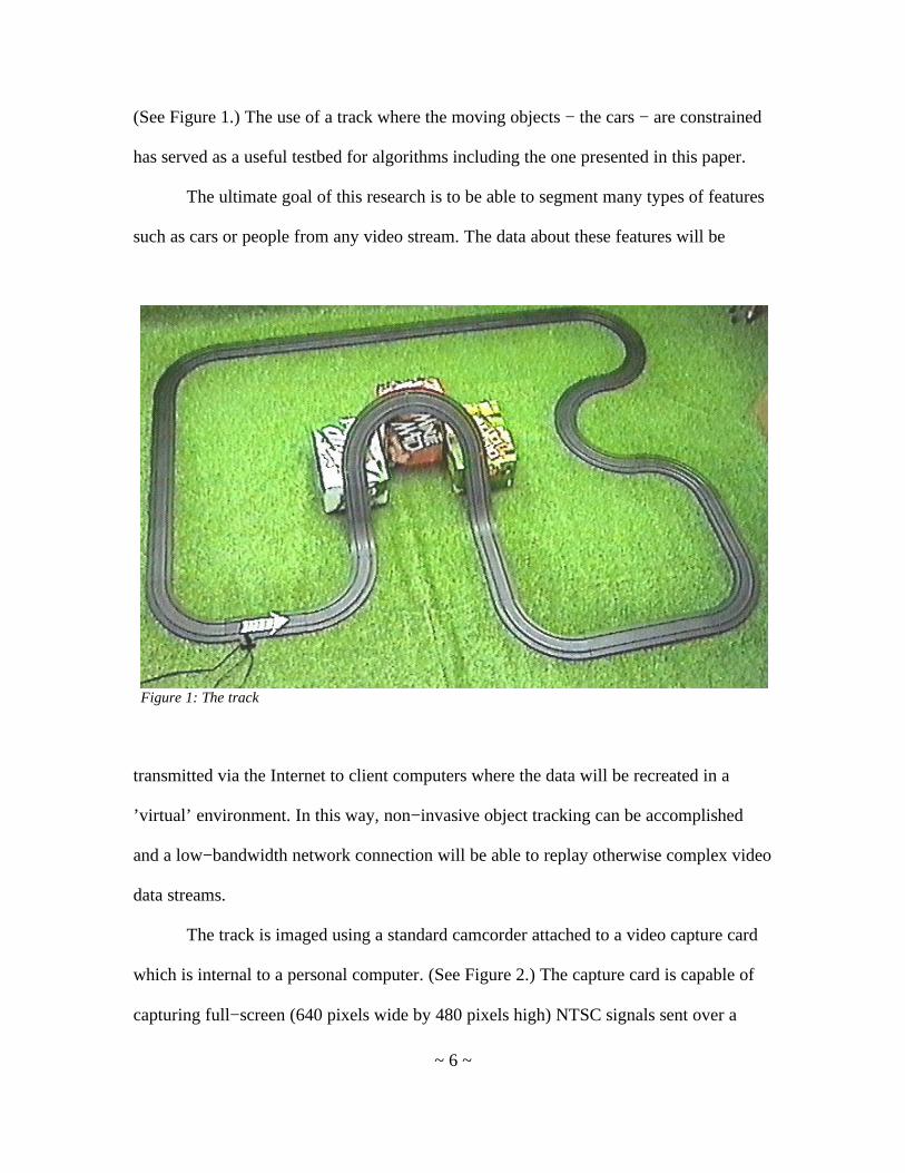
(See Figure 1.) The use of a track where the moving objects − the cars − are constrained

has served as a useful testbed for algorithms including the one presented in this paper.

The ultimate goal of this research is to be able to segment many types of features

such as cars or people from any video stream. The data about these features will be

transmitted via the Internet to client computers where the data will be recreated in a

’virtual’ environment. In this way, non−invasive object tracking can be accomplished

and a low−bandwidth network connection will be able to replay otherwise complex video

data streams.

The track is imaged using a standard camcorder attached to a video capture card

which is internal to a personal computer. (See Figure 2.) The capture card is capable of

capturing full−screen (640 pixels wide by 480 pixels high) NTSC signals sent over a

~ 6 ~

Figure 1: The track

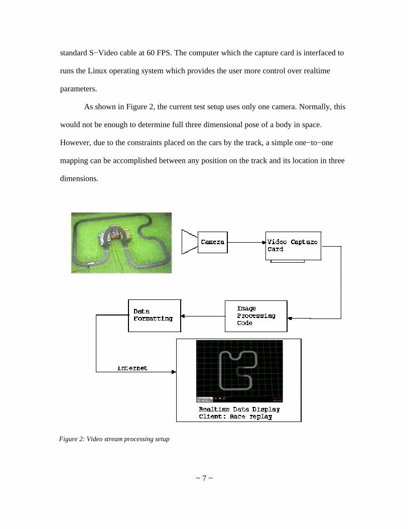
standard S−Video cable at 60 FPS. The computer which the capture card is interfaced to

runs the Linux operating system which provides the user more control over realtime

parameters.

As shown in Figure 2, the current test setup uses only one camera. Normally, this

would not be enough to determine full three dimensional pose of a body in space.

However, due to the constraints placed on the cars by the track, a simple one−to−one

mapping can be accomplished between any position on the track and its location in three

dimensions.

~ 7 ~

Figure 2: Video stream processing setup

Current Algorithms

The problem of recovering the full pose of an arbitrary number of cars on the

track in realtime has been solved using a combination of image processing algorithms.

The algorithm of note here is the one used determine the spatial location of the cars

without having to analyze the entire frame. Similar work has been done on unconstrained

objects [Rigoll].

Image Segmentation Algorithm

The most important algorithm is the one used to find the cars in a video frame −

the image segmentation algorithm. Remember that this needs to be accomplished in

under 33ms and the size of a still video frame is 640x480 pixels. The first step is to

subtract the background reference image − an image of the track with no cars on it −

from the still frame. Only new information − in this case the cars and spurious noise −

will appear. If the computer were fast enough, the entire frame could be analyzed and the

cars could be segmented out by use of a centroid−finding algorithm. However, it was

found that this approach would be wasteful and ultimately more expensive.

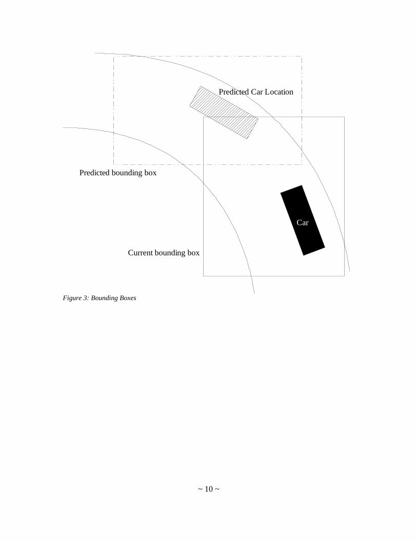
Bounding boxes

The solution to the problem of having to analyze the entire image was to use only

a small portion of the image. Ideally, that portion of the image would contain the car or

cars. By using this method, the analysis can be reduced from one of a 640x480−pixel

image to under 150x150 pixels. That is a reduction in space complexity of 92.7% and an

approximately corresponding reduction in time complexity.

The portion of the image to be analyzed is constrained by a what will be referred

to as a ’bounding box’. (See Figure 3.) The bounding box will follow the car around the

~ 8 ~

track and the image processing algorithms will operate inside the bounding box only.

There are two problems with this method: Firstly, the bounding box needs to start

tracking the car −’acquire’ it − at some initial point but without human intervention.

Secondly, the box must predict where the car will be in the next frame so as to follow it

around the track. The first problem is solved by placing a bounding box over some

arbitrary section of the track. It is made big enough to ensure that the car will at some

time in the future pass through the box. When it does, the box acquires the car and begins

to track it.

The second problem − to predict the future location of the car − is currently

solved with an educated guess: The algorithm knows that the car will move forward so it

projects the bounding box ahead on the track by a fixed length. Because the track has

turns and the cars change velocity, the bounding box must be made big enough to

encompass the error between the estimate and reality for the entire track. The purpose of

this paper is to present a way to localize the error, predict the future position of the car

with more accuracy, reduce the size of the bounding box and thereby reduce the time

needed to analyze a video frame.

~ 9 ~

~ 10 ~

Figure 3: Bounding Boxes

Current bounding box

Predicted bounding box

Car

Predicted Car Location

CHAPTER 2

IMPROVED BOUNDING BOX ALGORITHM

Summary

The use of a video stream provides extra information which does not exist in a

typical image processing application: time. The algorithm presented here uses the extra

information to predict the position and size of the bounding box. A Kalman filter and a

simple heuristic is used to do the prediction.

The Kalman Filter

The Kalman filter is a computationally efficient, recursive, discrete, linear filter.

It can give estimates of past, present and future states of a system even when the

underlying model is imprecise or unknown. For more on the Kalman filter there are

many good references available to explain it: [Welch00; Gelb74; Maybeck79]. The two

most important aspects of the Kalman algorithm are the system model and the noise

models. (Equations 1−5 describe the filter in one common way of expressing it.)

Table 1: Kalman filter time update equations (predict)

(1)

(2)

Table 2: Kalman filter measurement update equations (correct)

(3)

(4)

(5)

System Model

The system model used in this application is given by the state vector in Eq. 6.

~ 11 ~

´xk+1=Ak xk+Buk

Pk+1=Ak Pk AKT +Qk

K k=Pk HkT Hk Pk Hk

T+RkB1

xk=´xk+K zkBHk´xk

Pk= I BK k Hk Pk

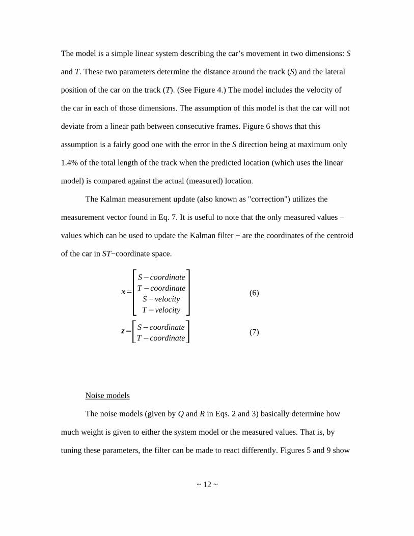
The model is a simple linear system describing the car’s movement in two dimensions: S

and T. These two parameters determine the distance around the track (S) and the lateral

position of the car on the track (T). (See Figure 4.) The model includes the velocity of

the car in each of those dimensions. The assumption of this model is that the car will not

deviate from a linear path between consecutive frames. Figure 6 shows that this

assumption is a fairly good one with the error in the S direction being at maximum only

1.4% of the total length of the track when the predicted location (which uses the linear

model) is compared against the actual (measured) location.

The Kalman measurement update (also known as "correction") utilizes the

measurement vector found in Eq. 7. It is useful to note that the only measured values −

values which can be used to update the Kalman filter − are the coordinates of the centroid

of the car in ST−coordinate space.

(6)

(7)

Noise models

The noise models (given by Q and R in Eqs. 2 and 3) basically determine how

much weight is given to either the system model or the measured values. That is, by

tuning these parameters, the filter can be made to react differently. Figures 5 and 9 show

~ 12 ~

x=

SBcoordinateTBcoordinate

SBvelocityTBvelocity

z= SBcoordinateTBcoordinate

the S and T measured values for a typical loop of a car around the track contrasted with

the predicted values. (The predicted values are given by the dashed line and the error

between the two curves in Figure 5 is shown in Figure 6 for more clarity.) Note that the

error in S is not obvious whereas the noise in T is highly visible. (Remember that the car,

because it is in a slot, should not change T position as it rounds the track. The obvious

noise is due to the inability of the imaging hardware to resolve the width of the track

with accuracy.)

To reduce the noise in the T coordinate, the noise parameters were manually

tuned to rely on the system model rather than the measured values. Figure 9 contrasts the

original noise in T to the filtered values. (The dashed line is the filtered data.) This is

~ 13 ~

Figure 4: The track coordinate system

S

T

Slots

simply an added benefit to using the Kalman filter − it makes the ultimate replay of the

data noticeably smoother.

Another parameter which was manually tweaked was the velocity of the car in the

T direction. Remember that because the car is in a slot, it is physically unable to move in

the T direction. Therefore the velocity in T should be near zero. As can be seen in Figure

8, it is not. Again, the noise model was manually tuned to smooth the T velocity. Figure

8 contrasts the filtered and unfiltered velocities with filtered velocity as a dashed line.

Equation 10, the measurement covariance noise matrix, shows quite graphically that the

measurement of the car’s position in the T coordinate is not to be trusted.

Final Kalman System Parameters

Equations 7−10 give the final parameters as implemented in code. The matrices

in Eqs. 7 and 8 are derived from the system model and measurement update equations,

respectively. The ∆t in Eq. 7 is the time between consecutive video frames − in this case

1/15 of a second. Equations 9 and 10 give the tuned process and measurement noise

covariance matrices, respectively. The prediction error covariance matrix P is initialized

to a 4x4 identity matrix.

~ 14 ~

(7)

(8)

(9)

(10)

Bounding Box Prediction

The ultimate goal of using the Kalman filter is to predict the size and position of a

bounding box which will be the only area of an image to be analyzed to find the car. To

do this prediction and to try to make the bounding box as small as possible − so as to

reduce computing time − we use the prediction made by the Kalman filter found in Eq. 1.

The prediction also includes an error covariance (P) given in Eq. 2. The prediction xk

gives us the center of the bounding box while the error covariance matrix gives a

’confidence’ measure of how good the estimated position is. Given that the confidence is

the variance (σ) of the S and T estimates, we can generate a bounding box based on the

variance and thus statistically model the likelihood of the car being positioned inside the

box in the next frame. However, to reduce complexity, the bounding box is simply made

+σ around the centroid of the predicted car in the T direction and +3σ in the S direction.

~ 15 ~

A=

1 0 ∆ t 0

0 1 0 ∆ t

0 0 1 00 0 0 1

H=1 0 0 00 1 0 0

Q=

1 0 0 00 10 0 00 0 1 00 0 0 10

∗0.01

R=1 00 20000

∗0.0001

A simple heuristic is used to make sure that the box can contain the car: if any dimension

of the box is smaller than the longest axis of the car as seen by the camera, that

dimension is changed to the longest axis of the car. In that way the box is assured of

being big enough to fit the car. Simulation found that extending the bounding box

forward only from the current position of the car (because the car can only move

forward) yields smaller boxes without sacrificing accuracy.

Effects of Misprediction

One added benefit of using the Kalman filter is that misprediction can be handled

gracefully. If the bounding box is mispredicted or the image segmentation algorithm

(used to find the car inside the bounding box) fails, not only will the next bounding box

get bigger because the error variance will increase but the filter’s prediction can be used

as the ’actual’ position of the car. Thus no missed frames will be noticed in the replay of

the race − it guarantees the framerate. It also gives some assurance of the bounding box

being correctly placed in the next frame to reacquire the car.

~ 16 ~

~ 17 ~

Figure 5: Comparison of predicted (dashed line) versus measured S−coordinate values

Time Index

S−

Co

ord

ina

te P

osi

tion

(in

che

s)

~ 18 ~

Figure 6: Difference between predicted and measured S−coordinate values

Time Index

Diff

ere

nce

(in

che

s)

~ 19 ~

Figure 7: Unfiltered and filtered (dashed line) velocity in the S direction

Time Index

Ve

loci

ty (

inch

es/

sec)

~ 20 ~

Figure 8: Unfiltered and filtered (dashed line) velocity in the T direction

Time Index

Ve

loci

ty (

inch

es/

sec)

~ 21 ~

Figure 9: Unfiltered and filtered (dashed line) car position in the T direction

Time Index

T−

Co

ord

ina

te P

osi

tion

(in

che

s)

CHAPTER 3

IMPLEMENTATION

Two implementations of the Kalman filter were written: one using MATLAB and

the other using Java. Figures 5−8 were generated using MATLAB. Appendix A lists the

relevant MATLAB code. To graphically illustrate the improved bounding box algorithm,

a Java applet originally designed as a data display tool was modified to display the

predicted bounding box. Figures 10 and 11 show two screenshots of the applet. Two cars

(represented by red and blue wireframe rectangular solids) are visible. The blue car’s

position is filtered. The red car is the measured (real) location of the blue car one step in

the future. A magenta bounding box created using the new algorithm is displayed. A

successful bounding box prediction places the entire red car inside the bounding box as

in Figures 10 and 11. Appendix B lists the Java Kalman filter code.

(Figures 10 and 11 show rectangular bounding boxes whose sides are vertical and

horizontal rather than angled. Doing this makes the boxes slightly bigger in terms of

pixel area but makes analysis of the inside of the box much simpler thus offsetting the

added size.)

~ 22 ~

CHAPTER 3

RESULTS

There are essentially two metrics with which to measure the performance of the

improved algorithm: bounding box size compared to the old algorithm and probability of

finding the car inside the predicted bounding box. Since the new algorithm has yet to be

integrated with the image processing code, all results herein are based on Java

simulations.

Bounding Box Size

Table 3 compares the bounding box sizes with the new algorithm and the old. The

new algorithm was implemented in simulation using car position data taken from the

same pre−recorded race as the old algorithm. The size of the bounding boxes decreased

by an average of 33.1%. It should be noted that the new algorithm provides more

flexibility in choosing box sizes and the user can choose whether they want smaller boxes

with a decrease in positioning accuracy or larger, conservative boxes which have a higher

likelihood of encompassing the car.

Table 3: Comparison of Bounding Box Sizes

Average Variance Datapoints

New Algorithm 2001.25 1190 276

Old Algorithm 2995.26 1141 3397

Probability of Finding the Car Inside the Predicted Bounding Box

Because the new algorithm was not implemented in the main image processing

~ 23 ~

code and therefore has not yet been tested in its intended environment, it would be

impossible to make a direct comparison between the accuracy of the new and old

algorithms at keeping the car inside the bounding box. Qualitatively the simulation shows

that the car never leaves the bounding box.

Conclusion

The simulations done on real data show that using a Kalman filter to predict the

future location of a car in a video stream is feasible. The combination of faster image

processing and the ability to recover from prediction or image analysis errors makes this

technique very attractive. The techniques used herein can even be applied to other

moving objects including those unconstrained by a track. In that case, the filter setup is

very similar to that described above.

~ 24 ~

~ 25 ~

Figure 10: Successful bounding box prediction

Figure 11: Successful bounding box prediction

References

Rigoll Gerhard Rigoll, Stefan Eickeler, Stefan Muller. Person Tracking inReal−World Scenarios Using Statistical Methods. Gerhard−Mercator−University Duisburg.

Welch00 Greg Welch and Gary Bishop. 2000. University of North Carolina−Chapel Hill Technical Report TR 95−041

Gelb74 Gelb, A. 1974. Applied Optimal Estimation, MIT Press, Cambridge,MA.

Maybeck79 Maybeck, Peter S. 1979. Stochastic Models, Estimation andControl, Volume 1, Academic Press, Inc.

~ 26 ~

APPENDIX A

MATLAB

% % TEST.M :%% Tests Kalman filtering of real ST−coordinate data from a file% and graphically displays the results% Patrick O’Malley% Nov. 2000%% Note: This is not a function so that the variables listed % below will be global after this code executes. It lets% you mess with the data post−processing%

clear x_predclear x_pred2clear xkclear st1clear vs1clear vt1clear zformat short format compact

l=278.586; % length of the track

% read the data file containing STST datam=dlmread(’newstst.dat’,’ ’);timestep = 1/15;

% st1 and st2 are the st datast1=m(:,1:2);

% hack the velocities −− very crudefor i=1:length(st1)−1 if st1(i+1) < st1(i) vs1(i,1) = (l−st1(i))+st1(i+1); else vs1(i,1) = st1(i+1)−st1(i); endend

for i=1:length(st1)−1 vt1(i,1)=st1(i+1,2)−st1(i,2);end

% vs1 and vs2 are the S−coord velocities (note that they are% off by one from the ST1 and ST2 matrices)vs1=vs1./timestep;vt1=vt1./timestep;

% I don’t want them to be off so I’ll cheat and copy the% first velocity twicevs1=[vs1(1);vs1];vt1=[vt1(1);vt1];

% initialize the matricesA=[1 0 timestep 0;0 1 0 timestep;0 0 1 0; 0 0 0 1];H=[1 0 0 0;0 1 0 0];

~ 27 ~

% P changes, Q and R are the noise matrices and % are considered to be constant. We initialize them to something% easy. Q=[1 0 0 0; 0 10 0 0; 0 0 20 0; 0 0 0 10]*.01; % process noiseR=[.01 0; 0 20000]*.0001; %measurement noiseP=eye(4); % error covariance

% the above P will be the initial error estimate% but we need an initial xkxk=[2 1.83 77 0.3]’;

for i=1:length(st1)

% solve the discontinuity problem by subtracting it out! if abs(st1(i,1)−xk(1,1)) > 200.0 xk(1,1)=xk(1,1)−l; end

% predict the state ahead xp = A*xk; PP = A*P*A’+Q; %PP

% x_pred2[] is the actual prediction, not the corrected one x_pred2(i,:) = xp’; % measurement update (correct) % find the Kalman gain K = P*H’*inv(H*PP*H’ + R); % make the z measurement matrix from true data z=[st1(i,1);st1(i,2)]; % and apply the correction to the predicted data xk=xp+K*(z−H*xp);

% and update the error covariance P = (eye(4)−K*H)*PP;

% for the sake of this experiment, put the % updated predictions in a vector x_pred(i,:)=xk’; end

x=1:1:200;

% plots for display: only the first 200 datapoints!

figure%subplot(3,2,1);% plot predicted versus measuredplot(x,x_pred2(2:201,1),’b−−’,x,st1(2:201,1),’r’);title(’predicted and measured: S values’);

%subplot(3,2,2);% plot the difference between predicted and measured Sfigureplot(x,x_pred2(2:201,1)−st1(2:201,1));title(’difference between predicted and measured: S values’);

%subplot(3,2,3);figureplot(x,vs1(1:200),’r’,x,x_pred2(1:200,3),’b−−’);

~ 28 ~

title(’Velocities in S’);

%subplot(3,2,4);figureplot(x,vt1(1:200),’r’,x,x_pred2(1:200,4),’b−−’);title(’Velocities in T’);

%subplot(3,2,5);figureplot(x, st1(1:200,2),’r’,x,x_pred2(1:200,2),’b−−’);title(’predicted and measured: T values’);

% write the predictions out%dlmwrite(’out2.dat’,[st1 x_pred2(:,1:2)],’ ’);

~ 29 ~

APPENDIX B

Java Code

/************************************************

KalmanFilter.java

Description: A simple Kalman filter class.

Author:Patrick O’Malley

Date:Nov. 2000

Notes:Must use the KalmanFilter.kalman()method and KalmanFilter.predict() methodtogether to get the right workings.

You need the Jampack −− the Java Matrixclasses −− to use this code.

*************************************************/

import Jampack.*;

public class KalmanFilter{

private Zmat P = null;private Zmat PP = null;private Zmat Q = null;private Zmat R = null;private Zmat A = null;private Zmat H = null;

public void setP( double[][] p ){

P = new Zmat(p);PP = new Zmat(p);

}

public void setQ( double[][] p ){

Q = new Zmat(p);}

public void setR( double[][] p ){

R = new Zmat(p);}

public void setA( double[][] p ){

A = new Zmat(p);}

public void setH( double[][] p ){

H = new Zmat(p);}

~ 30 ~

public Zmat getP() { return P; }public Zmat getQ() { return Q; }public Zmat getR() { return R; }public Zmat getA() { return A; }public Zmat getH() { return H; }

public Zmat kalman( Zmat xk, Zmat z ) throws JampackException{

// predict the state ahead//Zmat xp = Times.o( A, xk );//Zmat PP = Plus.o(Times.o(Times.o(A,P),Ctp.o(A)),Q);Zmat xp = xk;

// update the prediction (correct)Zmat temp = Inv.o( Plus.o( Times.o( Times.o( H,PP ),

Ctp.o(H)), R));Zmat K = Times.o(Times.o(P,Ctp.o(H)), temp);

Zmat innovation = Minus.o( z, Times.o(H,xp));Zmat output = Plus.o(xp, Times.o(K,innovation));

// update the error covarianceP = Times.o( Minus.o( Eye.o(4), Times.o(K,H)),PP);

return output;}

public Zmat predict( Zmat xk ) throws JampackException{

PP = Plus.o(Times.o(Times.o(A,P),Ctp.o(A)),Q);return Times.o( A, xk );

}

}

~ 31 ~