use of air conditioning heat rejection for swimming pool

Use of Air Conditioning Heat Rejection for Swimming Pool Heating

by

Sven-Erik Pohl

A thesis submitted in partial fulfillment of the requirements for the degree of

Master of Science

(Mechanical Engineering)

at the University of Wisconsin – Madison

1999

iii

Abstract

Residential swimming pools are common in Wisconsin. However, pool heaters are

needed in this climate to allow the pool to be used during the summer and to extend the

period of use from late spring to early fall. Swimming pool heaters commonly use natural

gas or propane as fuel. Although pool covers are often used to reduce the evaporation

loss, the heating needs of an outdoor pool can result in significant operating expense and

unnecessary use of natural resources. Even though the available solar energy is at a

maximum at the time that pool heating is needed, solar heating systems are not commonly

employed. Central air conditioning systems are common in Wisconsin. Central systems

are routinely installed in most new homes, especially in those that have residential

swimming pools. Air conditioners are electrically driven, and the energy removed from

the cooled space plus the electrical energy are rejected to the ambient through air-cooled

condensers. Even though the air conditioning season is relatively short in Wisconsin, air

conditioning is estimated to contribute 10 to 15 % to the electric demand in the state. The

objective of this study is to explore and evaluate different methods of combining air

conditioning and pool heating to reduce the energy requirements and electrical demand.

v

Acknowledgements

Special thanks go to my advisors John Mitchell and Bill Beckman for both their

assistance and their friendship. They were always patiently answering my various

questions and lead me to many new insights. Thank you for teaching me how to get down

to a problem and for all your motivation and help.

I would like to thank Sandy Klein for his assistance during my research and for

developing EES. It was never so EESy to get along with the English unit system!

My stay in Madison was made possible by the German Academic Exchange

Service (DAAD) and the Institut für Thermodynamik at the University of Hannover. I am

grateful to Prof. Kabelac and Dirk Labuhn for putting their personal effort in this program

to keep it running and to make this great study abroad experience possible.

The financial assistance for this project of William Heckrodt and the University of

Wisconsin Graduate School has been appreciated.

I am very grateful that I had the opportunity to complete my master degree at the

Solar Energy Laboratory. My time in the lab has been very intense and enjoyable. I really

appreciated the stimulating atmosphere in the lab. Thank you to all the people that I

worked with: Amr, Bryan, Florian, Janeen, Josh, Kyle, Mark, Mohammed, Rob and

Sherif. Our discussions solved many problems I encountered during my research. There is

vi

no way that I would have finished my work without Dave who helped me through my

struggles with TRNSYS as well as the daily hour of madness.

I am thankful to my friend and landlord Paul for answering all my questions

concerning language and culture. Thank you for teaching me all the necessary

vocabularies to survive outside the Engineering Research Building. I really enjoyed the

time I spend with Nils, who brought up new ideas and encouraged me to go my way.

Being abroad I learned to appreciate my good friends I have at home. Roman and

Andi, thank you for showing me that time and distance do not matter in a friendship.

I want to thank my parents and my sister Sonja for their support over the past 16

month. I am glad that you were able to visit me here in Madison and I am looking

forward to see you soon.

Finally very special thanks to Nicki who gave me the energy to get through every

day’s trouble. Thank you being patient with me in this long distance relation. Thanks for

being you.

vii

Table of Contents

Abstract iii

Acknowledgements v

Table of Contents vii

List of Figures xiii

Nomenclature xvii

Nomenclature xvii

Chapter 1

Introduction 1

1.1 Objective 1

1.2 An Introduction to TRNSYS 2

1.3 Softwa re Selection 5

Chapter 2

The Swimming Pool Simulation 7

2.1 Brief Literature Survey 7

2.2 A Comparison of Four Swimming Pool Simulations 9

2.2.1. Introduction 9

2.2.2. The different heat transfer mechanisms 11

2.2.3. Heat Losses 12

2.2.4. Heat Gains 12

2.2.5. Comparison of Four Computer Models 12

viii

2.2.5.1 POOLS (LBL) 12

2.2.5.2 F-Chart (F-Chart Software) 13

2.2.5.3 Energy Smart Pools Software (DOE) 13

2.2.5.4 TRNSYS TYPE 144 (Transsolar) 14

2.2.6. Evaporation Calculations 14

2.2.6.1 POOLS 9 (LBL) 14


2.2.6.3 Energy Smart Pools (DOE) 15


2.2.7. Comparison of the evaporation calculation methods 17

2.2.7.1 Effect of relative humidity 17

2.2.7.2 Effect of wind speed 20

2.2.8. Convection/Conduction Calculations 20

2.2.8.1 POOLS (LBL) 20




2.2.9. Comparison of the convection calculation methods 23

2.2.10. Wind Velocity 25

2.2.11. Sky Temperature 25

2.2.11.1 POOLS (LBL) 26

2.2.11.2 F-Chart Software and TRANSSOLAR 27

ix


2.2.12. Comparison of the radiation calculation methods 27

2.3 Summary 28

Chapter 3

The Air Conditioner Model 33

3.1 The Refrigeration Cycle 33

3.2 The Constant COP Model 33

3.3 The Variable COP Model 35


3.3.2. The Vapor-Compression Cycle 36

3.3.3. The Refrigerant 38

3.3.4. Performance of a Vapor-Compression Cycle 39

3.3.5. The Volumetric Compressor Efficiency Model 39

3.3.6. The Effectiveness-NTU Heat Exchanger Model 40

3.3.7. Fan and Pump 42

3.3.7.1 Fan Laws 42

3.3.7.2 Pump Modeling 43

3.4 The EES Air Conditioner Simulation 43


3.4.2. Calibration of the Simulation 44

3.4.3. A Fair Comparison 46

3.4.4. Implementation of the AC Model into TRNSED Simulation 48

x

3.4.5. Sensitivity Study for Temperature Approach 49

3.4.6. Generalization of the Air Conditioner Correlations 50

3.5 Summary 52

Chapter 4

Weather Data 55

4.1 Introduction 55

4.2 The Typical Meteorological Year (TMY and TMY2) 55

4.3 Generated Weather 56

4.4 Comparison of TMY Data and Generated Weather 56

4.5 Conclusions 59

Chapter 5

The Swimming Pool Air Conditioner (SPAC) 61

5.1 Introduction 61

5.2 SPAC Features 61

5.3 The SPAC Simulation 62

5.3.1. General Information 62

5.3.2. The Weather Data Mode 63

5.3.3. Adding TMY2 locations to the SPAC simulation 64

5.3.4. Swimming Pool Water Loss Calculations 64

5.3.5. Economic Analysis 65

5.4 The Building Simulation 66

5.4.1. Simple One-Zone Building with Attic 66

5.4.2. SPAC Building Input 67

xi

5.4.3. Adding a Building to the SPAC Program 68

5.5 The Swimming Pool 68

5.5.1. Base Case Swimming Pool Settings 69

5.6 The Air Conditioner 70

5.6.1. The Constant COP Model 70

5.6.2. The Variable COP Model 70

5.7 The Gas Pool Heater 71

5.8 Output 72

The Online Plotter 72

5.8.1. Output Files 73

Chapter 6

Simulation Results 75

6.1 Introduction 75

6.2 Swimming Pool Cover Control Strategies 75

6.2.1. Swimming Pool Covers 76

6.2.2. Comfort Swimming Pool Temperature 77

6.2.3. Effect of Swimming Pool Cover Control Strategies 77

6.2.4. Summary 82

6.3 Benefits for the Customer 83

6.3.1. System Control Strategies 83

6.3.2. Seasonal Operation Cost 85

6.3.3. Seasonal Savings for Different Locations 90

xii

6.3.4. Impact of Different Swimming Pool Sizes 91

6.3.5. Sensitivity of Deviation in Evaporation Calculation Methods 93

6.3.6. SPAC Equipment Cost 94

6.3.7. Air Conditioner Power Demand 97

6.3.8. Summary 98

6.4 Swimming Pool Water Level Calculations 98

Chapter 7

Conclusions and Recommendations 101

References 105

Appendix A

Description of TRNSYS Type 144 109

Appendix B

SPAC Output Files 117

Appendix C

SPAC Source Code 121

Appendix D

EES Air Conditioner Model 141

xiii

List of Figures

Figure 2.1 Heat transfer mechanisms associated with a swimming pool. 11

Figure 2.2 Comparison at different wind speeds and relative humidity of 1 18

Figure 2.3 Comparison at different wind speeds and relative humidity of 0.8 18



Figure 2.6 Convection losses with no pool cover for a relative humidity=0.6 and two

wind speeds 24

Figure 2.7 Radiation Losses from Uncovered Pool Surface 28

Figure 2.8 Total Energy Losses 30

Figure 3.1 A simple thermodynamic approach for an air conditioner 34

Figure 3.2 Schematic Diagram of a vapor – compression cycle 36

Figure 3.3 The pressure – enthalpy diagram for the vapor - compression cycle 37

Figure 3.4 The EES Diagram window provides a user- friendly input and output screen 44

Figure 3.5 Manufacturer data and simulation results agree within a small difference 45

Figure 3.6 Definition of the terminal temperature difference (TTD) for a condenser. 46

Figure 3.7 Performance of air conditioner simulation for water and air for different

temperature approaches. If the TTD increases, the performance decreases. 48

Figure 3.8 Seasonal Air Conditioning Savings for different temperature approaches 50

Figure 3.9 Application of the air conditioner correlations on different unit sizes 51

xiv

Figure 3.10 Effect of different air conditioner models on swimming pool temperature52

Figure 4.1 Monthly Average Ambient Temperatures for Generated Weather and TMY

Weather Data 57

Figure 4.2 Monthly Average Daily Global Horizontal Solar Radiation for Generated

Weather and TMY Weather Data. 57

Figure 4.3 Monthly Air Conditioning Cost Impacted by Generated Weather and TMY

Weather Data 58

Figure 5.1 General information window for SPAC 63

Figure 5.2 Radio buttons switch between the precipitation modes 65

Figure 5.3 Economics Analysis input mask in SPAC 65

Figure 5.4 Input mask of the building simulation in SPAC 68

Figure 5.5 Swimming Pool input mask in SPAC 69

Figure 5.6 Information required by the SPAC program for the Air Conditioner 71

Figure 5.7 Input Mask for the Gas Pool Heater in SPAC 71

Figure 6.1 US Cities that were examined for different pool cover strategies. 78

Figure 6.2 Swimming pool temperature for an uncovered and unheated pool 80

Figure 6.3 Temperature for an unheated and uncovered pool between 11am and 2pm 80

Figure 6.4 Pool temperature for a heated and part time covered pool 81

Figure 6.5 Automatic pool cover controlled swimming pool temperature 81

Figure 6.6 The Swimming Pool Air Conditioner Configuration 84

Figure 6.7 Cities for economic analysis 85

xv

Figure 6.8 Economic analysis for locations in different climates in the United States. For

each City the left column shows the conventional house cooling and heating,

while the right includes the swimming pool air conditioner plus additional

pool heating cost. 87

Figure 6.9 Electricity Cost for house cooling for a season between May 1st to October 1st

based on 0.075 $/kWh 88

Figure 6.10 Natural Gas Cost for swimming pool heating between May 1st to October 1st

based on 0.02 $/kWh 88

Figure 6.11 Electricity savings for SPAC compared to a conventional system for a season

from May 1st to October 1st based on 0.075 $/kWh 90

Figure 6.12 Natural Gas Savings for SPAC compared to a conventional system for a

season from May 1st to October 1st based on 0.02 $/kWh 91

Figure 6.13 Economic analysis for locations in different climates in the United States for a

27.5 m2 pool. 92

Figure 6.14 Economic analysis for locations in different climates in the United States for a

110 m2 pool. 92

Figure 6.15 Natural Gas Savings for different swimming pool sizes for a season between

May and November. 93

Figure 6.16 Impact of uncertainties in evaporation calculation methods on the natural gas

cost for the SPAC and conventional systems. 94

Figure 6.17 Incremental equipment cost for a SPAC system compared to a conventional

system because of better performance. Time period: May 1st to October 1st. 96

xvi

Figure 6.18 Power demand comparison for air conditioner systems. 97

xvii

Nomenclature

Roman Symbols

C Compressor clearance factor

Ci Cost for i

Cp Fan pressure coefficient

cp Heat capacity

Cv Fan capacity coefficient

Cw Fan power coefficient

COP Coefficient of performance

h Pool-air convection heat transfer coefficient

hpc Pool-Air convection heat transfer coefficient with cover

∆hevap Enthalpy of evaporation

LCC Life Cycle Cost

LCS Life Cycle Savings

•m Mass flow rate

N Isentropic exponent

NTU Number of transfer units

P Pressure

Pamb Saturation vapor pressure at ambient temperature

Patm Atmospheric pressure

Pdis Discharge pressure

Ppool Saturation vapor pressure at pool temperature

Ps Fan static pressure rise

Psuc Suction pressure

P1 Ratio of the life cycle fuel cost savings to the first-year fuel cost savings

xviii

P2 Ratio of the life cycle expenditures incurred to initial investment

∆PV Pressure drop

actQ•

Actual heat transfer rate

condQ•

Condenser heat transfer rate

evapQ•

Evaporative energy rate

max

•Q Maximum possible heat transfer rate

q”evap Evaporation heat flux

q”con Convection heat flux

Rbowen Bowen ratio

Rc R-Value of pool cover

Tamb Ambient temperature

Tc,i Cold fluid inlet temperature

Tcover Pool cover temperature

Tdp Dew point temperature

Th,i Hot fluid inlet temperature

Tpool Swimming pool temperature

Tsky Sky temperature

TTD Terminal temperature difference

U Fluid velocity

UA Overall heat loss coefficient

•V Fan capacity

wV•

Water loss per unit time

v Specific volume

vdis Specific suction volume

vG Mean wind velocity measured at ground level

vsuc Specific discharge volume

xix

vwind Mean wind velocity measured at weather station

•v Volumetric flow rate

disv•

Compressor displacement rate

•W Power

compW•

Compressor power

fanpumpW /

• Pump/fan power

Greek Symbols

ε Heat exchanger effectiveness

εs Cloudy sky emissivity

εsc Clear sky emissivity

δ Thickness of cover

ηvol Volumetric efficiency

ρ Density

σ Stefan Boltzmann constant

ξ Hydraulic loss figure

Additional Subscripts

e Electricity

eq Equipment

g Natural gas

SPAC Swimming pool air conditioner

1

Chapter 1 Introduction

1.1 Objective

In the Wisconsin climate residential swimming pools need to be heated through

out the season. Gas pool heaters are commonly used to supply the energy required to

maintain the comfort temperature of the swimming pool. However, most residences that

host a swimming pool nearby have air conditioning systems to reduce the temperature

inside the building. Consequently, there is one device that rejects heat and another one

that needs heat. The objective of this research is to explore and evaluate different methods

of combining air conditioning and pool heating to reduce the energy requirements and

electrical demand.

Both air conditioners and gas pool heaters require purchased energy to operate. If

the heating demand of the pool can be satisfied using the rejected heat from the building,

the gas energy for pool heating can be reduced or possibly eliminated. Additionally, a

water-cooled air conditioner performs better than a conventional air-cooled air

conditioner because of the water properties. Consequently, the homeowner saves

purchased energy by implementing a swimming pool heating system that uses the

swimming pool as the condenser for the air conditioner.

2

More than six million American families own a swimming pool. Consequently,

reducing the energy demand for pool heating and air conditioning helps saving natural

resources.

To investigate the performance of the improved swimming pool air conditioner

and to discuss the benefits of such a system, a computer simulation has been

implemented. A transient simulation program called TRNSYS was employed to simulate

the required components, where each component (building, air conditioner, swimming

pool) is based on equations that describe its physical behavior. This simulation can be

used for different places by changing the weather data, which is an input to the program.

It will be shown that the swimming pool air conditioner lowers the operation cost and

reduces the energy consumption for almost every location in the United States.

1.2 An Introduction to TRNSYS

TRNSYS is a transient system simulation program with a modular structure. The

program is well suited to simulate the performance of systems, the behavior of which is a

function of the passage of time. This is the case if outside conditions that influence the

system behavior change, such as weather conditions, or if the system components

themselves go through conditions that vary with time.

Modular simulation of a system requires the identification of components whose

collective performance describes the performance of the system. Each component is

formulated by mathematical equations that describe its physical behavior. The

mathematical models for each component are formulated in FORTRAN code, so that they

3

can be used within the TRNSYS program. Formulation of the components has to be in

accordance with the required TRNSYS format. A basic principle in this format is the

specification of PARAMETERS, INPUTS and OUTPUTS for each component.

Parameters are constant values that are used to model a component; these can be for

example, the geometric parameters of the swimming pool such as length, depth and

width. Inputs are time-dependent variables that can come from a user supplied data source

such as weather data or from outputs of other components.

There can be several components of the same type specified in one simulation.

The way this identification is accomplished is that each component is assigned an

identifying type number that is component specific. A second number, the unit number, is

unique an can only be used once in a simulation. Different unit numbers can be associated

with the same type number, although there are limitations on how many types of one kind

can be used in one simulation.

A system is set up in TRNSYS by means of an input file, called a TRNSYS deck.

This deck contains all the information that specifies the components and how the

components interact. The system is set up by connecting all inputs and outputs in an

appropriate way to simulate the real system. For example the cooling demand for the

building unit is the evaporator energy of the air conditioner unit. Once a system is set up

in a TRNSYS deck, the program can be run over a user defined time interval. The time

interval is divided into equal number of time steps. At each time step the program calls

each component and solves all the mathematical equations that specify the component

performance. The program iteratively calls the system component until a stationary state

4

is reached. The stationary state is reached when all the calculated inputs to the

components remain constant between two iterations. Naturally, in a numerical solution

such as calculated by TRNSYS, there will always be a difference in results between two

iterations. Therefore the user has to specify tolerances that define a stationary state.

Aside from the components that simulate actual physical parts of the system, there

are predefined utility components that can be used in the simulation. One of them is the

data reader. The data reader is able to read data from a user supplied data file that has to

be assigned in the TRNSYS deck. Every time step of the simulation the data file then

reads the desired values from the file and makes them accessible to the components.

Another kind of utility component is a printer that stores output data in a file.

Several printers can be defined in one deck. These output files can be imported into a

spreadsheet program and the results further examined. The online plotter can be used to

make the progress of the simulation visible on the screen, so that the user can

immediately decide whether a run was useful or not. Additionally, a quantity integrator is

available to integrate values over time.

A special feature of the TRNSYS program package is the possibility to create a

user-friendly input file called a TRNSED file. When the TRNSED program is started, the

user only has to supply the important parameters and can change these easily for different

simulations. In this way the program is accessible to users who are not experienced in

using TRNSYS but are only interested in examining a particular system.

5

1.3 Software Selection

Based on the features mentioned in section 1.2, TRNSYS was selected as the

primary tool to perform the swimming pool air conditioner analysis.

Although the main product of the present work is a swimming pool air conditioner

simulation in TRNSYS appearing in user-friendly TRNSED format, parts of the studies

were done using EES (Engineering Equation Solver). The basic function provided by

EES is the solution of a set of algebraic equations. EES can also solve differential

equations, equations with complex variables, do optimization, provide linear and non-

linear regression and generate plots. The program was especially useful for the

examination of the refrigeration cycle because of its built-in thermophysical property

functions. A Diagram window provides a place to display important input and output

values and a schematic diagram can help to interpret their meaning.

7

Chapter 2 The Swimming Pool Simulation

2.1 Brief Literature Survey

The following section gives an overview of some of the studies found in the

literature that discuss the energy transfer across an air water interface for large bodies of

water, such as a swimming pool.

Carrier (1918) did a series of measurements on pans and small tanks in wind

tunnels where the evaporation rate was formulated in terms of the partial pressure

difference of water and the air above it, and the velocity of the air.

Ryan and Harleman (1973) introduced a study of transient cooling pond behavior

and developed an algorithm to simulate the thermal and hydraulic behavior of a cooling

pond or lake. They gave relations to estimate the surface energy flux. The convective

energy transfer terms were divided into a forced and free convection part. The forced

convection was estimated by an empirical function. The free convection terms were

derived from a basic heat and mass transfer analogy for a flat plate. The flat plate

relations were refined by accounting for the effect of the water vapor in the air above the

surface. A so called wind function was introduced, that combined free and forced

convection effects. Relations to estimate long wave radiation from the water to the sky

were also given in the study of Ryan and Harleman.

8

The American Society of Heating, Refrigeration and Air Conditioning Engineers

Handbook ASHRAE (1991) uses the Carrier equations but notes that the equation, when

applied to swimming pools, may predict high values for the heat loss.

Wei, Sigworth et al. (1979) performed a swimming pool analysis. This analysis

gives a relation for heat and mass transfer across a pool surface that is similar to the one

proposed by Ryan and Harleman, but neglects the effect of water vapor in the air with

respect to free convection. Estimations of radiation heat transfer are also made.

Smith, Loef et al. (1994) made measurements on the evaporation losses from an

outdoor swimming pool by measuring the reduction of pool water volume over time due

to evaporation as well as measuring evaporation losses from pans floated in the pool.

They also measured the temperature change of the pool and correlated the heat loss with

the evaporation and measured the radiation exchange between the pool surface and the

sky. The data were analyzed and compared to the commonly used evaporation rate

equations found in the ASHRAE Applications Handbook. The result found was lower

than the predicted result by ASHRAE and a modified version of the ASHRAE equation

was developed.

Hahne and Kuebler (1994) made measurements on two heated outdoor swimming

pools located in Stuttgart, Germany. They applied formulas for evaporation, radiation,

convection, conduction and fresh water supply developed by Richter (1969), Richter

(1979) to predict the heat balance of the pools. Using the most suitable correlation for the

evaporative losses of the pool the temperature was found to have less than 0.5 K standard

9

deviation between measured and simulated temperature. The result was implemented in a

TRNSYS subroutine (TYPE 144).

2.2 A Comparison of Four Swimming Pool Simulations

2.2.1. Introduction

The following comparison of four different computer programs for simulating

swimming pools has been made in an attempt to find the most reliable model for

swimming pool heat losses. The emphasis of the comparison is on evaporation models

since evaporation accounts for such a large percentage of the heat loss. All of these

programs are based on measurements made on pools, lakes or ponds. In each case the

measured results were used to find model parameters so that the model and measurements

agree. In spite of this experimental verification of the programs, the programs predict

different evaporative losses. Part of this difference may be due to the very different nature

of the experiments as discussed below.

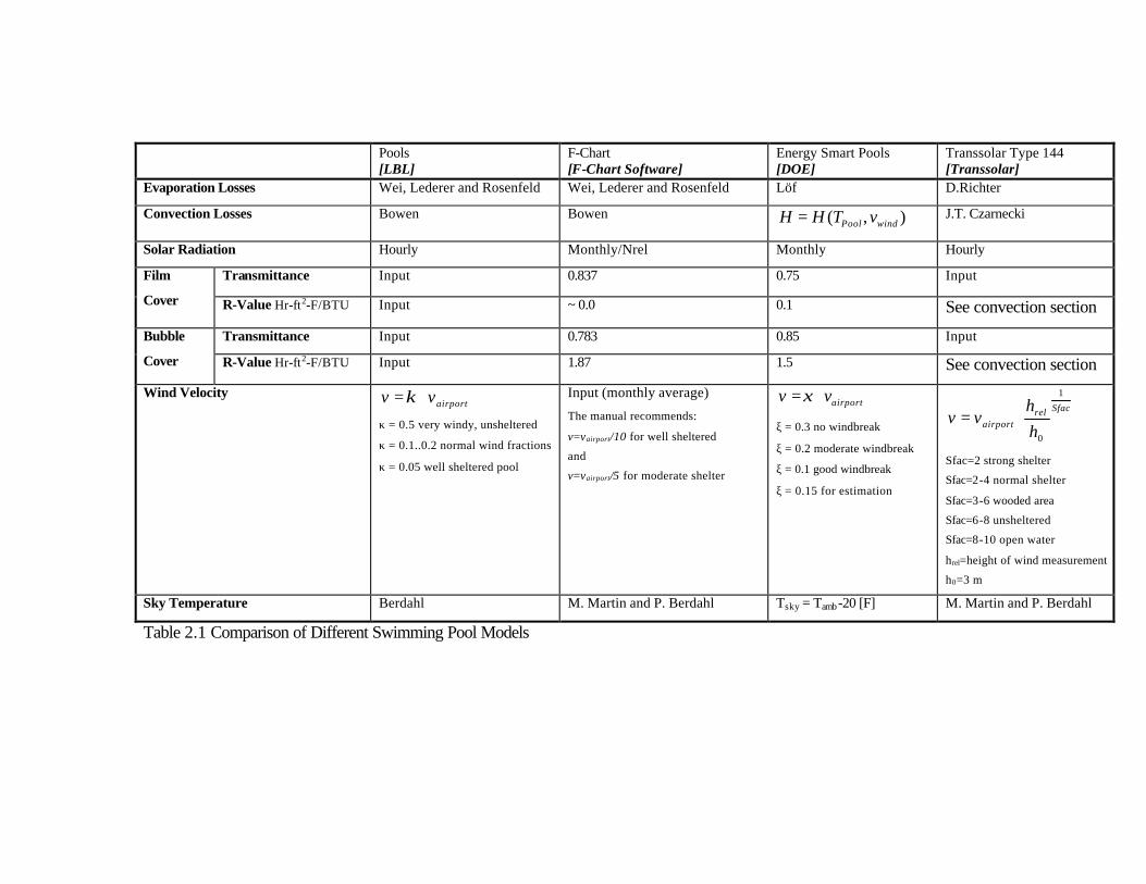
Table 2.1 provides an overview of the algorithms used in the various programs for

convection, evaporation and radiation. Information is also provided on how each program

obtains certain thermal parameters. For example, the cover transmittance for solar

radiation is a program input (i.e., set by the user) for POOLS and TRANSSOLAR but is a

fixed, but different, value for F-Chart and ESP. The following sections give an overview

of the four programs and then discuss the various assumptions in more detail.

Pools [LBL]

F-Chart [F-Chart Software]

Energy Smart Pools [DOE]

Transsolar Type 144 [Transsolar]

Evaporation Losses Wei, Lederer and Rosenfeld Wei, Lederer and Rosenfeld Löf D.Richter

Convection Losses Bowen Bowen ),( windPool vTHH = J.T. Czarnecki

Solar Radiation Hourly Monthly/Nrel Monthly Hourly

Transmittance Input 0.837 0.75 Input Film

Cover R-Value Hr-ft2-F/BTU Input ~ 0.0 0.1 See convection section

Transmittance Input 0.783 0.85 Input Bubble

Cover R-Value Hr-ft2-F/BTU Input 1.87 1.5 See convection section

Wind Velocity airportvv ⋅=κ

κ = 0.5 very windy, unsheltered

κ = 0.1..0.2 normal wind fractions

κ = 0.05 well sheltered pool

Input (monthly average)

The manual recommends:

v=vairport/10 for well sheltered

and

v=vairport/5 for moderate shelter

airportvv ⋅=ξ

ξ = 0.3 no windbreak

ξ = 0.2 moderate windbreak

ξ = 0.1 good windbreak

ξ = 0.15 for estimation

Sfacrelairport h

hvv

1

0

⋅=

Sfac=2 strong shelter

Sfac=2-4 normal shelter

Sfac=3-6 wooded area

Sfac=6-8 unsheltered

Sfac=8-10 open water

hrel=height of wind measurement

h0=3 m

Sky Temperature Berdahl M. Martin and P. Berdahl Tsky = Tamb-20 [F] M. Martin and P. Berdahl

Table 2.1 Comparison of Different Swimming Pool Models

11

2.2.2. The different heat transfer mechanisms

To predict the pool energy use, an energy balance is set up that specifies the heat

fluxes through the water surface. Table 2.1 shows schematically the heat gains and losses

from a pool. Both the ESP and F-Chart programs use monthly average energy balances

that ignore the thermal capacitance of the pool. The POOLS and TRYSYS programs use

hourly energy balances that include the thermal capacitance of the pool. In all the

programs the energy gains that increase water temperature come from the direct sun, a

solar collector, or a gas (typically) pool heater. The energy losses that decrease the water

temperature come from convection, evaporation and radiation to the ambient. Conduction

to the ground is small and is neglected in all of the programs.

DirectSunHeat LossesLosses Solar

CollectorGas PoolHeater

Heat Losses to the Ground

EvaporationConvection

Radiation

Heat GainsGains

Figure 2.1 Heat transfer mechanisms associated with a swimming pool.

12

2.2.3. Heat Losses

Of the three heat losses from an uncovered pool the most important is evaporation,

often accounting for 45-60% of the total loss. The convection loss is a function of wind

speed above the water surface, which is difficult to estimate and the difference in water

vapor pressure between the ambient air and the pool surface. The radiation heat loss from

the pool to the sky is also difficult to estimate due to problems with estimating the

effective sky temperature. All three of these heat losses can be reduced by means of pool

covers whenever the pool is not used.

2.2.4. Heat Gains

The largest heat gain is due to the incoming solar radiation, approximately 80% of

which is absorbed by the water. Using a solar heater with a collector area that is 75% of

the pool area can nearly double the amount of solar energy available to the pool, as noted

by Wei, Sigworth et al. (1979).

2.2.5. Comparison of Four Computer Models

2.2.5.1 POOLS (LBL)

The computer program called POOLS has been developed by Wei, Sigworth et al.

(1979) at the Lawrence Berkeley Laboratory (LBL) to compare a wide range of pool

energy conservation measures including pool covers and solar collectors. The computer

simulations are reported to agree with measurements within a range of 10%. To determine

13

the accuracy of the computer model, heating gas requirements of existing pools were

simulated, using the model, and compared with actual gas consumption in the San

Francisco bay area. The solar system gains to the pool are based on hourly calculations of

the collector performance. The program source code is no longer available but the

algorithms used in the program are available in the LBL report by Wei, Sigworth et al.

(1979).

2.2.5.2 F-Chart (F-Chart Software)

The F-Chart Software (Beckman, Klein et al. (1977)) is a program based on

methods developed by S. A. Klein and W. A. Beckman. The F-Chart solar design method

(Beckman, Klein et al. (1977)) was developed to select the size and type of solar collector

that, in conjunction with an auxiliary furnace, will supply the entire heating load at the

least possible cost. The solar collector performance is based upon utilizability methods

developed by Klein and Beckman and reported by Duffie and Beckman (Beckman, Klein

et al. (1977)). Results of the POOLS program were used in the development of the F-

Chart program.

2.2.5.3 Energy Smart Pools Software (DOE)

The Energy Smart Pools Software (Gunn, Jones et al. )), developed by the U.S.

Department of Energy (DOE), is designed to estimate the annual cost of heating both

indoor and outdoor swimming pools and spas. The software is designed to analyze energy

and water savings from pool covers and solar pool heating systems. It can also be used to

14

determine differences between conventional heating and high efficiency heating systems

and conventional and high efficiency electric motors. The calculation of the solar gain

from the solar collector system is based upon a monthly average day. If the collector has a

high loss coefficient, as might be expected of an uncovered collector, then this method of

estimating collector performance can lead to significant errors.

2.2.5.4 TRNSYS TYPE 144 (Transsolar)

TRNSYS (Klein (1996)) is a transient system simulation program with a modular

structure. The modular structure of TRNSYS gives the program tremendous flexibility,

and facilitates the addition to the program of models not included in the standard library.

The TYPE 144 (Auer (1996)) is a non-standard TRNSYS model which was developed by

the TRANSSOLAR Company in Stuttgart, Germany, to simulate an outdoor or indoor

swimming pool. The solar system model is similar to that used by the POOLS program in

that the collector output is calculated on an hourly basis.

2.2.6. Evaporation Calculations

2.2.6.1 POOLS 9 (LBL)

The evaporative heat flux due to combined forced and free convection was

obtained from Wei, Sigworth et al. (1979). This algorithm is a result of a study by Klotz

(1977) at Standford and Ryan and Harleman (1973), at MIT. Wei, Lederer and Rosenfeld

verified these algorithms with measurements on pools in the San Francisco bay area.

15

( )

⋅⋅−⋅

⋅−

+−⋅−

+⋅+⋅⋅=

psiinHg

PP

PP

T

P

PT

vq

ambpool

atm

amb

amb

atm

pool

poolwindLBLevap

035859.2

378.01

460

378.01

4605692540417.0"

31

, ( 2.1 )

Where

q”evap = Evaporation heat flux [BTU/hr-ft^2]

Ppool = saturation vapor pressure at the pool temperature [psia]

Pamb = saturation vapor pressure at the ambient temperature [psia]

Patm = atmospheric pressure, typically 14.7 [psia]


The F-Chart Software uses the same evaporation equation used by Wei, Sigworth

et al. (1979) implemented in the LBL computer program. However, as F-Chart is a

monthly average program, it uses a monthly average ambient temperature and relative

humidity.

2.2.6.3 Energy Smart Pools (DOE)

Energy Smart Pools (Gunn, Jones et al. )) uses the evaporation algorithm reported

in Smith, Jones et al. (1993): Evaporation rates are based on an experimental study of an

indoor pool. Based on a single indoor pool experiment, the energy loss rates were set to

be 74% of that predicted by the Carrier equation (Carrier (1918)) used in the ASHRAE

16

Applications Handbook (ASHRAE (1982)). The Carrier algorithm was developed from

measurements on a small shallow pond in an outdoor environment. It is difficult to make

any judgment as to how the wind velocity in this indoor environment relates to the wind

in an outdoor environment.

( ) ( )

⋅⋅−⋅⋅+=

psiainHg

PPvCCq ambpoolwindESPevap 035859.2" 21, ( 2.2 )

Where:

q”evap,esp = Evaporation Heat Flux [BTU/hr-ft2]

vwind = Wind Speed [mph]

P = Pressure [psia]

C1 = 69.4 [Btu/hr-ft2-inHg]

C2 = 30.8 [Btu/hr-ft2-inHg-mph]


TRNSYS TYPE 144 (Auer (1996)) uses an empirical correlation based on a report

by Richter (1969), who investigated evaporation losses on a cooling pond in Germany.

( )

⋅⋅

⋅⋅

⋅−⋅

⋅⋅⋅+⋅=

2

2

,.

5.0

,

//

08805508.0

44704.052.5639.426.3"

mhrKJhrftBtu

PrelhumPmph

smvq ambdwpooldwwindTranssolarevap

( 2.3 )

Where:

( ) 9/532' ⋅−= poolpool TT ( 2.4 )

17

( ) 9/532' ⋅−= ambamb TT ( 2.5 )

[ ]

⋅⋅

⋅×+⋅−+= −

atmkPa

TTTP poolpoolpoolpooldw

325.101

'102200.7'00000352.0'0007109.0004802.0 372,

( 2.6 )

[ ]

⋅⋅

⋅×+⋅−+= −

atmkPa

TTTP ambambambambdw

325.101

'102200.7'00000352.0'0007109.0004802.0 372,

( 2.7 )

2.2.7. Comparison of the evaporation calculation methods

In Figures 2-5, the evaporative heat flux is shown versus the ambient temperature.

The pool water temperature is chosen to be a constant at 27°C. The plots are arranged

with increasing relative humidity (40 to 100%) and in each chart the wind speed was

chosen to be either 0 or 3.2 km/h.

2.2.7.1 Effect of relative humidity

For a relative humidity (RH) of 100% and an ambient temperature of 27°C the

evaporation for all methods is zero, because in this point the ambient temperature and the

pool water temperature are the same and the difference in relative humidity is zero.

18

Relative Humitity = 1, Swimming Pool Temperature = 26.6 C

0

50

100

150

200

250

300

350

400

10 12 14 16 18 20 22 24 26 28

Ambient Temperature [C]

Eva

po

rati

on

Hea

t L

oss

[W

/m^2

]Richter (Trnsys) @ v = 3.2 km/h

Wei (Pools, F-Chart) @ v =3.2 km/h

Löf (ESP) @ v = 3.2 km/h

Richter (Trnsys) @ v = 0 mph

Löf (ESP) @ v = 0 km/h

Lof (ESP) @ v = 0 km/h

Evaporation Heat Loss Comparison for Different Wind Velocities

Figure 2.2 Evaporation Comparison at different wind speeds and relative humidity of 1

Relative Humitity = 0.8, Swimming Pool Temperature = 26.6 C

0

50

100

150

200

250

300

350

400

10 12 14 16 18 20 22 24 26 28


Eva

po

rati

on

Hea

t L

oss

[ W

/m^2

]

Richter (Trnsys) @ v = 3.2 km/h



Richter (Trnsys) @ v = 0 km/h

Wei (Pools, F-Chart) @ v =0 km/h



Figure 2.3 Evaporation Comparison at different wind speeds and relative humidity of 0.8

19


0

50

100

150

200

250

300

350

400

10 12 14 16 18 20 22 24 26 28


Eva

po

rati

on

Hea

t L

oss

[W

/m^2

]Richter (Trnsys) @ v = 3.2 km/h









0

50

100

150

200

250

300

350

400

10 12 14 16 18 20 22 24 26 28


Eva

po

rati

on

Hea

t L

oss

[W

/m^2

]

Richter (Trnsys) @ v = 3.2 km/h

Wei (Pools, F-Chart) @ v =3.2 km/hLöf (ESP) @ v = 3.2 km/h





20

From Figure 2.2 to Figure 2.5, at a constant ambient temperature and decreasing

RH, all three methods predict an increase in the evaporation energy loss. For a pool with

zero wind speed, the Richter (TRANSSOLAR) and the Löf (ESP) models have

essentially the same slope but the Löf algorithm predicts about 30% higher heat loss than

the Richter model. The Wei (LBL) curve crosses both the Richter and Löf curves for all

of the different relative humidities.

2.2.7.2 Effect of wind speed

With the relative humidity held at 60% the heat transfer predicted by the Richter

(TRANSSOLAR) and Löf (ESP) yields by a factor of 2 between a wind speed of 0 and

3.2 km/h. On the other hand the Wei (LBL) correlation varies by a factor of only 1/3. For

a wind speed of 3.2 km/h the Löf (ESP) model gives the highest evaporation heat loss as

the Wei model (LBL) is constantly about 70 W/m² lower than the Löf.

2.2.8. Convection/Conduction Calculations

2.2.8.1 POOLS (LBL)

Bowen (1926) related the heat loss by conduction directly to the evaporation heat

loss, by considering the process of molecular diffusion from a water surface in the

presence of forced convection. This leads to

LBLevapbowenLBLcon qRq ,, "" ⋅= ( 2.8 )

21

and Rbowen is known as the Bowen Ratio

92.2901.0 atm

ambpool

ambpoolbowen

PPP

TTR ⋅

−−

= ( 2.9 )

Where:

q”con, LBL = Convection Heat Flux [Btu/hr-ft2]

Ppool = Saturated Water Vapor Pressure at Tpool [inHg]

Pamb = Water Vapor Pressure at Tamb [inHg]

Tpool = Pool Temperature [F]

Tamb = Ambient Temperature [F]


The F-Chart program uses the same equations used in the LBL model*.


Convection losses are calculated as a function of a convection coefficient and pool

water temperature – air temperature difference. The convection coefficient is a function

of pool surface wind speed as given by:

( ) ( )drybulbpoolpcESPcon TTherherq −⋅⋅−+⋅= %cov1%cov" , ( 2.10 )

* Eqn (9.7.2) in Solar Engineering of Thermal Processes, by J. A. Duffie and W. A.

Beckman is in error. The coefficient 0.0006 should be 0.00022.

22

and

hR

h

c

pc 115.0

1

++=

( 2.11 )

Gvh ⋅+= 3.01 ( 2.12 )

windG vv ⋅= 15.0 ( 2.13 )

Where:

q”con,ESP = Hourly Convection Energy Load [Btu/hr]

Cover% = Pool Area Covered [%]

Tpool = Pool Temperature [F]

Tdrybulb = Dry Bulb Temperature of Air [F]

hpc = Pool-Air Convection Coefficient with Cover [F]

h = Pool –Air Convection Heat Transfer Coeff. [Btu/hr-ft2-F]

vG = Mean Wind Velocity Measured at Ground Level [mph]

vwind = Mean Wind Velocity Measured at Weather Station [mph]

Rc = R-Value of Pool Cover [hr-ft2-F/Btu]


The TRNSYS model uses a switch to change between a covered and uncovered

pool. In the case of an uncovered pool (cover% = 0) the heat loss is a convection loss, and

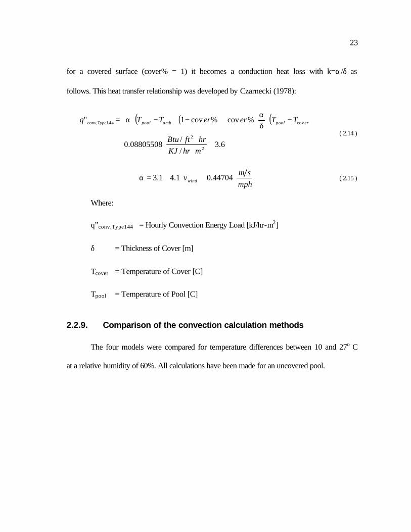
23

for a covered surface (cover% = 1) it becomes a conduction heat loss with k=α/δ as

follows. This heat transfer relationship was developed by Czarnecki (1978):

( ) ( ) ( )

6.3//

08805508.0

%cov%cov1"

2

2

cov144,

⋅

⋅⋅⋅⋅

−⋅

δα⋅+−⋅−⋅α=

mhrKJhrftBtu

TTererTTq erpoolambpoolTypeconv

( 2.14 )

⋅⋅⋅+=αmph

smvwind 44704.01.41.3 ( 2.15 )

Where:

q”conv,Type144 = Hourly Convection Energy Load [kJ/hr-m2]

δ = Thickness of Cover [m]

Tcover = Temperature of Cover [C]

Tpool = Temperature of Pool [C]

2.2.9. Comparison of the convection calculation methods

The four models were compared for temperature differences between 10 and 27o C

at a relative humidity of 60%. All calculations have been made for an uncovered pool.

24

0

20

40

60

80

100

120

10 12 14 16 18 20 22 24 26 28Ambient Temperature [C]

Co

nve

ctio

n H

eat L

oss

[W/m

^2]

Type 144 (Transsolar) @ v =0 [km/h]

ESP (DOE) @ v =0 [km/h]

Pools (LBL) @ v =0 [km/h]

Type 144 (Transsolar) @ v =3.2 [km/h]

ESP (DOE) @ v =3.2 [km/h]

Pools (LBL) @ v =3.2 [km/h]

Convection Heat Loss Comparison for DifferentWind VelocitiesRelative Humidity = 0.6, Swimming Pool Temperature = 26.6 C

Figure 2.6 Convection losses with no pool cover for a relative humidity=0.6 and two wind

speeds

The F-Chart program also uses the Bowen ratio that is implemented in the LBL

model.

The Bowen method takes a temperature difference and vapor pressure difference

into account to calculate the heat flux due to the convection whereas the ESP and

TRANSSOLAR programs use only the temperature difference. All four models consider

the wind speed as a variable. The TRANSSOLAR predictions vary by 100% when the

changes from 0 to 3.2 km/h. The ESP model is relatively insensitive to different wind

velocities. The change predicted by the LBL model is between that predicted by the other

two methods. At 27 oF the ambient temperature and the pool temperature are equal and all

convective losses are zero.

25

2.2.10. Wind Velocity

In all of the programs the wind speed to use in the evaporation and convection

loss terms is related to the wind speed at the airport. Table 2.1 gives the relationships

between the airport wind speed and the local wind speed. The TRANSSOLAR program

permits the user to input wind speed measurements at any height. In the other programs a

standard “airport measurement height” is assumed. In the TRANSSOLAR program an

exponential form is used to convert the airport measurement to local value with 5 levels

of shelter. In the other programs a linear “airport reduction factor” is used that typically

varies from 0.1 to 0.2 although the POOLS program suggests 0.5 for unsheltered areas

and the ESP program suggests 0.3 for no windbreak. At this time it is unclear how these

adjustments were determined. Furthermore, by selecting different wind speeds (or

“airport reduction factors”), for the different programs, the evaporation and convection

correlations can be made to agree for most conditions. There is insufficient experimental

information available to pick one correlation over the other.

2.2.11. Sky Temperature

The radiation exchanged between the pool surfaces and the ambient is a function

the pool and sky temperatures and the pool emittance. A gas (and consequently the

atmosphere) has the ability to emit and absorb radiation. The so-called “sky temperature”

is an equivalent radiation temperature to be used in a simple two-body radiation problem.

This sky temperature is not equal to the ambient temperature. The sky is considered to be

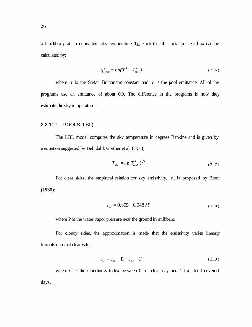
26

a blackbody at an equivalent sky temperature Tsky such that the radiation heat flux can be

calculated by:

)TT("q skyrad44 −εσ= ( 2.16 )

where σ is the Stefan Boltzmann constant and ε is the pool emittance. All of the

programs use an emittance of about 0.9. The difference in the programs is how they

estimate the sky temperature.

2.2.11.1 POOLS (LBL)

The LBL model computes the sky temperature in degrees Rankine and is given by

a equation suggested by Behrdahl, Grether et al. (1978):

414 )T(T ambssky ε= ( 2.17 )

For clear skies, the empirical relation for sky emissivity, εs is proposed by Brunt

(1938):

P..sc 04806050 +=ε ( 2.18 )

where P is the water vapor pressure near the ground in millibars.

For cloudy skies, the approximation is made that the emissivity varies linearly

from its nominal clear value.

( ) Cscscs ⋅ε−+ε=ε 1 ( 2.19 )

where C is the cloudiness index between 0 for clear day and 1 for cloud covered

days.

27

2.2.11.2 F-Chart Software and TRANSSOLAR

Both methods calculate the sky temperature by using the equation developed by

Martin and Behrdahl (1984)

412 1501300000730005607110 )]tcos(.T.T..[TT dpdpambsky ⋅⋅+⋅+⋅+= ( 2.20 )

Where Tsky and Tamb are in degrees Kelvin, Tdp is the dew point temperature in

degrees Celsius and t is the hour from midnight. This equation is based on experimental

data that covered a temperature range from –20 to +30 degrees Celsius.


The Energy Smart Pools Program estimates the sky temperature to be the air temperature

minus 20 degrees F.

2.2.12. Comparison of the radiation calculation methods

The radiative heat fluxes shown in Figure 7 vary between 90 and 190 W/m2 for a

pool temperature of 10o C and between 5 and 110 W/m2 for a pool temperature of 27o C.

Only TRANSSOLAR and F-Chart use humidity sensitive equations and they vary as

shown. For most conditions the ESP and LBL programs predict lower values than the F-

Chart and TRANSSOLAR programs. The LBL predictions approach zero at Tamb=Tpool,

which is clearly incorrect. F-Chart and TRANSSOLAR use the more recent LBL sky

temperature correlations, which generally predicts a higher radiation heat loss than ESP.

28

0

20

40

60

80

100

120

140

160

180

200

10 12 14 16 18 20 22 24 26 28


Rad

iatio

n H

eat L

oss

[W/m

^2]

ESP (DOE)

Pools (LBL)

F-Chart & Type 144 @ RH=0.4



F-Chart & Type 144 @ RH=1

Radiation Heat Loss Comparison for Different Relative Humidities

Swimming Pool Temperature = 26.6 C

Figure 2.7 Radiation Losses from Uncovered Pool Surface

2.3 Summary

To compare the four computer simulations, all losses from an uncovered outdoor

swimming pool have been added up and the fractions of evaporation, radiation and

convection were evaluated as a function of ambient temperature. The relative humidity

was set to 60 %. Figure 2.8 shows the predicted heat losses from all four computer

models at two different wind speeds. As expected the energy lost increases at increasing

wind speed and decreasing ambient temperature. The trends are similar for all of the

programs but the magnitudes are different.

The highest loss without wind is calculated by the F-Chart program and is about

440 W/m2. For a wind of 3.2 km/h the TRANSSOLAR and ESP programs predict the

29

highest heat loss of about 570 W/m2 at 10 degrees Celsius and 220 W/m2 at 27 degree

Celsius.

For no wind the evaporation heat flux behaves very similarly in the correlations

used in the ESP, LBL, and the F-Chart model. The TRANSSOLAR program estimates

the evaporative losses to be somewhat lower than the other programs. The ESP model for

a wind velocity of 3.2 km/h calculates the highest evaporation loss. The evaporative

losses for ESP are higher than f-chart while the TRANSSOLAR evaporative losses are

smaller than f-chart at zero wind speed and about the same as f-chart at a 3.2 km/h wind

speed. With the large uncertainty in estimating the evaporative losses, and with no

definitive experiments available to test the predictions, it is unclear which algorithm

should be used. All models show the same characteristics and about the same magnitude

for the convective heat loss. At zero wind speed TRANSSOLAR predicts the smallest

convection loss and at 3.2 km/h TRANSSOLAR predicts the largest convection heat loss.

Since the convection heat loss in all of the programs is small relative to the evaporation

and radiation heat losses, the algorithm choice does not make much difference in the

overall heat loss. Perhaps the most surprising result is the variation in the radiation heat

loss predicted by the four programs. The different assumptions made for the sky

temperature have a very significant impact on the radiative losses.

30

Figure 2.8 Total Energy Losses

31

The LBL program used a version of the sky temperature developed by Martin and

Berdhal in 1978 but this algorithm was modified in 1984, after the POOLS program was

developed. The 1984 algorithm is used in both the F-chart and TRANSSOLAR programs

and predicts the highest radiative heat flux from the pool surface to the surroundings. The

assumption of using Tamb minus 20 oF for the sky temperature, as used in ESP program,

appears to underestimate radiative losses.

Since the overall losses are relatively equal and the correlations behave similar

there is no advantage of choosing one approach over the other. For further studies the

TYPE 144 developed by the TRANSSOLAR Company has been used to model the

swimming pool because it was already available as a subroutine for TRNSYS.

33

Chapter 3 The Air Conditioner Model

3.1 The Refrigeration Cycle

For the purpose of this research two different air conditioner models were

developed. First, an approach using a constant coefficent of performance (COP) was

applied, because house and building temperatures are nearly constant (since the pool is

heated). Also, it will be shown for energy observations concerning the swimming pool a

constant COP model is suffiencent. Second, when examining the energy consumption of

an air conditioner that rejects heat either to the ambient air or to the swimming pool

water, it is important to have a more precise model in order to be able to obtain a

temperature sensitive result. This leads to an air conditioner model that has a COP as a

function of the condenser inlet temperature and therefore allows more precise economic

observations. The following section describes the components of both the constant and

the variable COP model.

3.2 The Constant COP Model

As a first approximation for the air conditioner model, a simple thermodynamic

approach was used where the coefficient of performance was assumed to be constant.

34

Figure 3.1 shows an idealized refrigeration system described by energy fluxes into the

system boundary at certain temperatures of Tpool and Thouse.

•W

condQ•

poolT

evapQ•

houseT

Figure 3.1 A simple thermodynamic approach for an air conditioner

For the present work evapQ•

is the building cooling demand and condQ•

the amount

of energy added to the pool.

Performance of a refrigeration cycle is usually described by a coefficient of

performance. The COP is defined as ratio of the amount of removed heat to the required

energy input to operate the cycle

•

•

==W

Q

pliedenergy sup Neteffect trefrigeran Useful

COP evap ( 3.1 )

Applying the first Law of Thermodynamics for the system in Figure 3.1 yields:

evapcond QWQ•••

−= ( 3.2 )

Combining ( 3.1 ) and ( 3.2 ) leads to an equation that is only a function of the

building cooling demand and the COP. By fixing the COP and calculating the cooling

demand of the building the energy rejected to the swimming pool can be obtained by the

following equation:

35

−−=

••

COPQQ evapcond

11

( 3.3 )

The constant COP model that was built into the Swimming Pool Air Conditioner

Simulation is based on the single equation model given by equation ( 3.3 ). It was found

that for energy balance purposes of the swimming pool the constant COP model

sufficiently predicts the air conditioner behavior. For further information see paragraph

3.5.

3.3 The Variable COP Model

3.3.1. Introduction

In order to obtain detailed information on the system performance as a function of

environmental impacts a more precise model of a vapor compression air conditioner was

modeled using EES (Engineering Equation Solver). The standard thermodynamic

approach was used where the pressure drop in the evaporator and the condenser were

neglected and the isentropic compressor efficiency was assumed to be constant. To

transfer thermal energy from an enclosure such as a refrigerator or a building it is

necessary to have a fluid that has the ability to absorb the energy from one area and reject

it to another area, usually through condensation and evaporation. The first and second

laws of thermodynamics can be applied to individual components to determine mass and

energy balances and the irreversibility of the components.

36

3.3.2. The Vapor-Compression Cycle

Vapor-compression cycles are most common in air conditioning systems today. A

general illustration of a vapor-compression cycle is shown in Figure 3.2. The pressure-

enthalpy diagram visualizes the phase changes throughout the process Figure 3.3

Condenser

Valve

Compressor

T C, out

T C, in T E, out

T E, in

W comp

� �

� �

Evaporator

•

Figure 3.2 Schematic Diagram of a vapor – compression cycle

The evaporator, where the desired refrigeration effect is achieved, was chosen to

start the analysis. As the refrigerant passes through the evaporator, heat transfer from the

refrigerated space results in the vaporization of the refrigerant.

37

Figure 3.3 The pressure – enthalpy diagram for the vapor - compression cycle

For a control volume enclosing the refrigerant side of the evaporator, the mass and

energy rate balances reduce to give the rate of heat transfer per unit mass of refrigerant

flow

( )4141 hhmQ −⋅=••

( 3.4 )

where •m is the mass flow rate of the refrigerant. The heat transfer rate 41

•Q is

referred to as the refrigerant capacity. The refrigerant leaving the evaporator is

compressed to a relatively high pressure and temperature by the compressor. Assuming

no heat transfer to or from the compressor, the mass and energy balances for a control

volume enclosing the compressor give

38

( )1212 hhmW −⋅=••

( 3.5 )

where 12

•W is the power input to the refrigeration cycle. Because the enthalpy at

state 2 remains unknown, an isentropic compression can be assumed to calculate an ideal

compressor work and is later corrected by the compressor efficiency to derive the actual

compressor work.

Next, the refrigerant passes through the condenser, where the refrigerant

condenses and heat is transferred from the refrigerant to the cooling fluid, which is

usually air or water. For a control volume enclosing the refrigerant side of the condenser,

the rate of heat transfer of the refrigerant is

( )2323 hhmQ −⋅=••

( 3.6 )

Finally the refrigerant enters the expansion valve and expands to the evaporator

pressure. This process is usually modeled as a throttling process, for which

43 hh = ( 3.7 )

The refrigerant pressure increases in the irreversible adiabatic expansion, and

there is an accompanying increase in specific entropy. The refrigerant exits the valve at

state 4 as a two-phase liquid-vapor mixture.

3.3.3. The Refrigerant

The refrigerant is the working fluid for an air conditioning cycle. Although the

Montreal Protocol, which controls the production of ozone-depleting substances,

prescribes a phase-out of HCFC (Hydrochloroflourocarbons) in the next 30 years, the

39

HCFC R22 is still used in air conditioning systems in the U.S. To be able to calibrate a

computer model and to compare results HCFC R22 has been used for the computer

simulation.

3.3.4. Performance of a Vapor-Compression Cycle

As shown in equation ( 3.1 ) the coefficient of performance is defined as the ratio

of net energy that is supplied to the system to the work that is needed to run the cycle. For

a mechanical vapor compression system, the net energy supplied is usually in form of

work, mechanical or electrical, and may include work to the compressor and fans or

pumps.

fanpumpcomp

evap

WW

QCOP

/

••

•

+= ( 3.8 )

3.3.5. The Volumetric Compressor Efficiency Model

The compressor efficiency is not constant for all conditions. The effect will be

shown in the following section.

The compressor refrigerant flow rate is a decreasing function of the pressure ratio

due to the re-expansion of the vapor in the clearance volume. With the refrigerant vapor

modeled as an ideal gas, the volumetric flow rate is given in the ASHRAE Fundamentals

Handbook ASHRAE (1997) by the following:

40

−+=

•• n

suc

disdis

P

PCCvv

1

1 ( 3.9 )

where v is the volume flow rate, disv is the displacement of the compressor, C is

the clearance factor ( cylinderclearance vv ), sucdis PP is the cylinder pressure ratio and n the

polytropic exponent.

The volumetric compressor efficiency is defined as ratio of the volume flow rate

to the compressor displacement rate and is therefore affected by equation ( 3.9). Applying

the definition for polytropic expansion and compression

pvn=const ( 3.10 )

the volumetric efficiency can be calculated by

−⋅−=η 11

dis

sucvol v

vC

( 3.11 )

3.3.6. The Effectiveness-NTU Heat Exchanger Model

The evaporator and the condenser heat exchangers are modeled using the

effectiveness-NTU method. The effectiveness of the heat exchanger is defined as the ratio

of the actual heat transfer for a heat exchanger to the maximum possible heat transfer rate

max

•

•

=εQ

Q act ( 3.12 )

where the maximum heat transfer is

41

( )icihp TTmcQ ,,min

max −⋅

⋅=

••

( 3.13 )

where min

⋅

•mc p is the minimum of the heat capacity and mass flow rate product

for either the hot or the cold fluid.

The number of transfer units (NTU) is a dimensionless parameter that is widely

used for heat exchanger analysis and is defined as

minCUA

NTU = ( 3.14 )

where min

min

⋅=

•mcC p and UA is the overall heat loss coefficient.

From these equations the effectiveness-NTU relation can be determined for

different heat exchanger designs and were found in Incropera and DeWitt (1985). For a

counterflow arrangement the effectiveness is

( )( )r

r

CCNTU

−−−−

=ε1

1exp1

( 3.15 )

where max

min

CC

Cr = ( 3.16 )

For heat exchangers in which condensation occurs, the temperature remains

constant and ∞→hC . Conversely, in an evaporator it is the cold fluid that experiences a

change in phase and remains at a nearly uniform temperature ( )∞→cC . In that case the

value of Cr is defined to be zero and for all heat exchangers the effectiveness is calculated

by

42

( )NTU−−=ε exp1 . ( 3.17 )

3.3.7. Fan and Pump

For completeness in the evaluation of the coefficient of performance the fan and

pump work have to be included into the calculations.

3.3.7.1 Fan Laws

Residential split air conditioners usually have a fan built into their outdoor unit

that blows air through the condenser to achieve the desired condensing effect. The fan

characteristics can be described by three relationships that predict the effect on fan

performance of changing such quantities as the density of the air (ρ), operating speed (N),

and size of the fan (d). These equations are known as the fan laws and can be found in

Roberson and Crowe (1985):

3dNCV V ⋅⋅=•

( 3.18 )

ρ⋅⋅⋅= 22 dNCP Ps ( 3.19 )

ρ⋅⋅⋅=•

53 dNCW W ( 3.20 )

•V is the capacity, SP is the static pressure rise and

•W is the power. The various

coefficients ( VC - capacity coefficient, PC - pressure coefficient, WC - power coefficient)

can be determined for a fixed diameter, speed and inlet air density taken from

manufacturer data.

43

3.3.7.2 Pump Modeling

The swimming pool water is moved through the condenser by a pump. For flow

through pipes the Bernoulli Equation can be applied:

••⋅∆= VPW V ( 3.21 )

2

2uPV ⋅ρ⋅ς=∆

( 3.22 )

•W is the pump power, VP is the is the pressure drop because of friction,

•V is the

volumetric flow, ς is the hydraulic loss figure, ρ is the density of water and u is the

velocity. Again, the model can be validated by applying manufacturer data for a pump.

The hydraulic loss figure is assumed to be unity for corroded pipes.

3.4 The EES Air Conditioner Simulation

3.4.1. Introduction

A useful engineering tool, the Engineering Equation Solver (EES), was employed

to solve the coupled non-linear equations governing an air conditioning system. Besides a

fast algorithm EES provides property data for refrigerants and other species, that make

the calculations much easier. Additionally a diagram window, as shown in Figure 3.4, can

be used to present the results in a window that may include a graphic of the simulated

process. In this work the main diagram window provides an overview about input and

output variables. Two child windows carry information of the pump and fan settings.

44

Sven's Air Conditioner

T1=3.481 [C]T2=86.02 [C]

T3=50.63 [C] T4=3.481 [C]

P1=556.3 [kPa]P2=1970 [kPa]

P3=1970 [kPa] P4=556.3 [kPa]

W =4.039 [kW ]

UAcond=0.8439 [kJ/s-K] UAevap=1.014 [kJ/s-K]

TE,out=11.48 [C]

TE,i n= 22 [C]TC,out=35.63 [C]

TC,IN= 25 [C]

COP=2.898EER=9.887

Eva

po

rato

r

D= 0.004 [m3/s]

εcond=0.4147 εevap=0.568

ηcomp= 0.7

NTUcond=0.5357 NTUevap=0.8393

Qcond=16.75 [kJ/s] Qevap=12.71 [kJ/s]

R22Refrigerant:

m=0.08918 [kg/s]

Solar Energy Laboratory - Sven-Erik Pohl 1999

[12 C < Tc,in <40 C ]

AirCondenser Cooling Fluid :

15∆T=T3 -Tc,out =∆Tai r= 15

∆Twater= 5.5

mcond=1.565 [kg/s]

8∆Tevap=Te,out-T ,1 =

mevap= 1.2 [kg/s][Set for Pump/ Fan individually]

Figure 3.4 The EES Diagram window provides a user-friendly input and output screen

The objective of the EES program is to study the changes in the coefficient of

performance for the different cooling fluids of the condenser. A conventional air

conditioner rejects the energy to the ambient air that is moved through the heat exchanger

by a fan. The air conditioner that transfers the condenser heat to the swimming pool uses

water as cooling fluid. The idea is to generate curve fits of the coefficient of performance

versus condenser inlet temperature, i.e. the pool temperature. To simulate the air

conditioner curve fits were also developed for the change in the capacity as a function of

the condenser inlet temperature.

3.4.2. Calibration of the Simulation

To achieve results that reflect the real behavior of a conventional residential air

conditioner the EES simulation was calibrated using manufacturer performance data. The

45

available information covered performance and capacity data as a function of the

condenser coolant inlet temperature. Also, the fan parameters were taken from catalog

data and the building conditions were fixed. Two simulation parameters, the compressor

displacement rate and the compressor efficiency, were varied to minimize the error in

COP between catalog data and simulation results.

10 15 20 25 30 35 40 45 502.0

2.5

3.0

3.5

4.0

4.5

5.0

5.5

TC,IN [C]

CO

P

Simulation Results versus Catalog Data

COPsimulationCOPsimulation

COP=7.156839 - 0.1673290·CET[i] + 0.00142934·CET[i]2

COP=7.156839 - 0.1673290·CET[i] + 0.00142934·CET[i]2

COPcatalogCOPcatalog

Figure 3.5 Manufacturer data and simulation results agree within a small difference

Figure 3.5 shows the four data points given by manufactures catalog data and the

simulation results after the minimization. A curve fit represents the catalog data over the

temperature range of interest. The behavior as given in the catalog can be predicted

within a small error.

46

3.4.3. A Fair Comparison

A major problem was how to make a fair comparison of a conventional air-cooled

air conditioner to a water-cooled air conditioner. Manufacturers data are available for

residential air conditioners, but for a swimming pool air conditioner such information is

not available. Properties such as the heat exchanger effectiveness or the overall heat loss

coefficient were examined but led always to the problem that there is no information for a

water-cooled system. Finally the terminal temperature difference (TTD) was taken to

compare the different systems, because values were available from air conditioner

designer experience. The approximate values for the terminal temperature difference are

assumed to be about 10 C for air and 5.5 C for water.

T C, out

T C, in

�

�

Refrigerant

Water/ Air

�

�

TTD

Figure 3.6 The definition of the terminal temperature difference (TTD) for a condenser.

The TTD is the temperature difference between the condenser cooling fluid outlet

temperature and the condensation temperature of the refrigerant. Figure 3.6 shows the

definition of the TTD for the vapor-compression cycle described above. The variation in

the terminal temperature differences for water and air is based on their properties and

different mass flow rates through the heat exchanger. Naturally, water performs better

47

than air in a heat exchanger. Thus, by changing the working fluid of the condenser the

terminal temperature difference changes. It is also necessary to include the designer

knowledge of the mass flow rate. The TTD for water of 5.5 C goes along with a water

flow rate of 36 cm3/s per kW of refrigeration effect. Accordingly, a 10 kW air conditioner

would have a water flow rate of 360 cm3/s and a TTD of 5.5 C.

The temperature approach was used to run calculations for a range of condenser

cooling fluid inlet temperatures for both, water and air. The performance of the two

systems (water-cooled and air-cooled) can be seen in Figure 3.7. For a better

understanding, a change in the TTD can be explained as a change in the physical size of

the heat exchanger. In other words, a smaller heat exchanger results in a larger TTD.

Therefore, for an increasing TTD for water, which means a decreasing heat exchanger

size, the performance is decreasing.

By comparing a water-cooled heat exchanger with a large temperature difference

to an air-cooled heat exchanger with a small temperature difference a condition can be

found were both air-cooled and water-cooled perform the same.

48

10 15 20 25 30 35 40 45 502.0

2.5

3.0

3.5

4.0

4.5

5.0

5.5

6.0

6.5

7.0

7.5

TC,in [C]

CO

P

Air, ∆Tair= 10 CAir, ∆Tair= 10 C




Sensetivity Study - Impact of Temperature Approach on COP


Water, ∆Twate r = 5.5 CWater, ∆Twate r = 5.5 C




Air, ∆Tai r= 14 CAir, ∆Tai r= 14 C

Water, ∆Twater = 3.5 CWater, ∆Twater = 3.5 C


CopaCopa

CopwCopw

Figure 3.7 Performance of air conditioner simulation for water and air for different temperature

approaches. If the TTD increases, the performance decreases.

As the condenser inlet temperature increases the performance decreases. That

means the hotter the ambient conditions the more energy consumed by the air conditioner.

Ironically, an air conditioner performs best when its not needed.

3.4.4. Implementation of the AC Model into TRNSED Simulation

The air conditioner model has been analyzed in EES but the transient system

simulation is to be performed in TRNSYS. Consequently, it is necessary to implement the

results from the EES model into TRNSYS. The best realization would be to take the

equations from the EES program and use them in a TRNSYS Type. Unfortunately a

number of iterations are needed to solve for the system equation resulting in a significant

49

solution time. This fact makes it difficult to transfer the EES simulation into TRNSYS.

For this purpose another feature of EES was used – the results were transferred using

curve fits. These curve fits were combined in a way that for each TTD the coefficient of

performance and the capacity can be determined. In Figure 3.7 the result is shown for the

desired TTD’s of 5.5C and 10C. Curve fits of the coefficient of performance and the

capacity as the function of the condenser inlet temperature were implemented in a Fortran

subroutine. This subroutine is then called by the TRNSYS, which returns information

about the air conditioner performance.

3.4.5. Sensitivity Study for Temperature Approach

In order to investigate the sensitivity of a change in the TTD the TRNSYS model

was run for a range of terminal temperature differences. Figure 3.8 presents the result by

showing the seasonal savings as a function of the TTD for water and air. The savings are

based on the difference between the cost of an air-cooled system and a water-cooled

system over the time period of May 1st and October 1st. It can be seen that the savings for

the proposed approach of 5.5 C for water and 10 C for air would be about $36 of air

conditioner operation cost. Assuming an uncertainty of ±10 % in the TTD the amount of

saved money differs about ± $5, which is about 14 % of the original savings.

50

1.0 2.0 3.0 4.0 5.0 6.0 7.0 8.0 9.0 10.0 11.0 12.02

3

4

5

6

7

8

9

10

11

12

Term inal Temperature Difference - W ater [C]

Ter

min

al T

emp

erat

ure

Dif

fere

nce

- A

ir [

C]

-10

0

10

20

30

40

50

Seasonal Savings for Different Heat Exchanger Designs for Water and Air

Dec

reas

ing

Air

-Co

ole

d H

eat E

xch

ang

er S

ize

Decreasing Water-Cooled Heat Exchanger Size

Seasonal Air Conditioning Savings in US$

based on 0.075 $/kWh

1st March through 1st October

for Madison, WI

(Cost Air-Cooled AC - Cost Water-Cooled AC)

Figure 3.8 Seasonal Air Conditioning Savings for different temperature approaches

3.4.6. Generalization of the Air Conditioner Correlations

To make the correlations for coefficient of performance and capacity suitable for

other air conditioners than the one employed in this work the equations have been

normalized by dividing the correlations by their corresponding value at a rating

temperature of 35 C. The rating temperature is a standard rating point for air conditioners

tested using the Air-Conditioning and Refrigerant Institute’s (ARI) rating system. The

Air-Conditioning and Refrigeration Institute (ARI) provides a certification program for

unitary air conditioners in their ARI 210/240-89 Norm. The idea is that a user of the

51

TRNSYS program enters the performance values for his specific air conditioner that has

been tested under ARI conditions and the program itself doesn’t have to be changed.

25 30 35 40 45 502.0

2.5

3.0

3.5

4.0

Condenser Inlet Temperature Tc,in [C]

Co

effi

cien

t o

f P

erfo

rman

ce (

CO

P)

[-]

Carrier 38CKB060

Model 38CKB060Model 38CKB060

Carrier 38TDA060Carrier 38TDA060

Model 38TDA060Model 38TDA060

Carrier 38BR030Carrier 38BR030

Model 38BR030Model 38BR030

Performance: Manufacturer Data and Simulation Results

Figure 3.9 Application of the air conditioner correlations on different unit sizes

Figure 3.9 shows a comparison of different air conditioner manufacturer data and

the fitted correlations. The plot indicates that the generalization of the correlations is

limited. It works fine for the original set of data but for other unit sizes it only can give an

approximate performance map. An objective for future research could be an investigation

of a better way to generalize the gained air conditioner correlations.

52

3.5 Summary

In this section two air conditioner models were presented. The first model is based

on a simple thermodynamic approach that assumes a constant coefficient of performance.

It was found that this one-equation simulation is sufficient to predict the swimming pool

temperature.

To obtain information about the energy consumption of a water-cooled air

conditioner a second more detailed model was implemented that calculates the

performance and the capacity of two cooling fluids, water and air based on the condenser

inlet temperature and the terminal temperature difference.

0

5

10

15

20

25

30

35

40

2880 3640 4400 5160 5920 6680

Time [Hrs]

Sw

imm

ing

Poo

l Tem

pera

ture

[C]

Variable COP Model

Constant COP Model

Madison WiMay st to October 1st

Figure 3.10 Effect of different air conditioner models on swimming pool temperature

Figure 3.10 shows a comparison of the constant COP model and the variable COP

model. It can be seen that there is no effect on the swimming pool temperature although

53

the two models have a different performance and do not deliver the same amount of heat

to the pool.

For predicting the swimming pool temperature the changes due to a varying COP

can be neglected. But for an economic analysis, a more detailed model needs to be used,

because of the sensitivity of the power demand of the air conditioner to changes in the

COP.

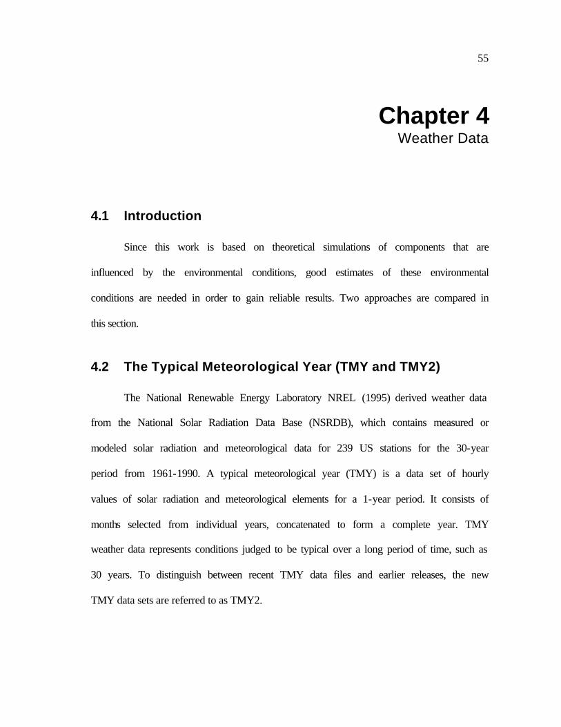
55

Chapter 4 Weather Data

4.1 Introduction

Since this work is based on theoretical simulations of components that are

influenced by the environmental conditions, good estimates of these environmental

conditions are needed in order to gain reliable results. Two approaches are compared in

this section.

4.2 The Typical Meteorological Year (TMY and TMY2)

The National Renewable Energy Laboratory NREL (1995) derived weather data

from the National Solar Radiation Data Base (NSRDB), which contains measured or

modeled solar radiation and meteorological data for 239 US stations for the 30-year

period from 1961-1990. A typical meteorological year (TMY) is a data set of hourly

values of solar radiation and meteorological elements for a 1-year period. It consists of

months selected from individual years, concatenated to form a complete year. TMY

weather data represents conditions judged to be typical over a long period of time, such as

30 years. To distinguish between recent TMY data files and earlier releases, the new

TMY data sets are referred to as TMY2.

56

4.3 Generated Weather

For some locations only monthly average weather information is available. To

allow hourly simulations for places with limited weather data, a TRNSYS TYPE

“Weather Generator” has been developed by Knight, Klein et al. (1991). This component

generates hourly weather data given the monthly average values of solar radiation, dry

bulb temperature, humidity ratio and wind speed. The data are generated in a manner such

that their associated statistics are approximately equal to the long-term statistics at the

specified location. The purpose of this method is to generate a single year of typical data,

similar to a Typical Meteorological Year.

4.4 Comparison of TMY Data and Generated Weather

For the purpose of this study, the TMY2 data and the generated weather set have

been compared to check the agreement of both methods. For locations in the US, the

TMY2 weather data set provides almost as much information as the generated weather.

However, the file size for the generated data is much smaller than TMY2 data files. For

example, the whole data file for the weather generator that includes 329 locations has

only 91 kByte compared to 1.2 Mbytes for one location of TMY2 data.

For a fair comparison, of the generated weather is based on monthly average

ambient temperatures and monthly average solar radiation values obtained from TMY2

weather data for Madison, WI. These monthly average data are inputs to the weather

generator.

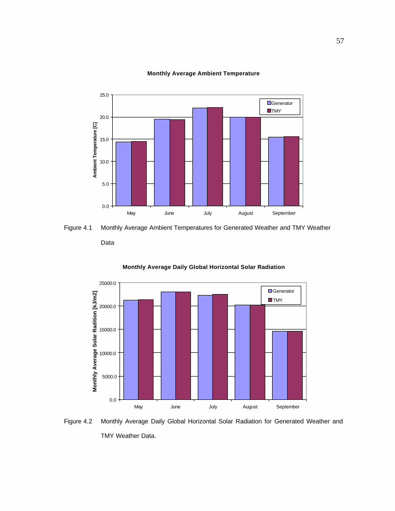
57

Monthly Average Ambient Temperature

0.0

5.0

10.0

15.0

20.0

25.0

May June July August September

Am

bien

t Tem

pera

ture

[C]

Generator

TMY

Figure 4.1 Monthly Average Ambient Temperatures for Generated Weather and TMY Weather

Data

Monthly Average Daily Global Horizontal Solar Radiation

0.0

5000.0

10000.0

15000.0

20000.0

25000.0


Mo

nth

ly A

vera

ge

So

lar

Rad

itio

n [

kJ/m

2] Generator

TMY

Figure 4.2 Monthly Average Daily Global Horizontal Solar Radiation for Generated Weather and

TMY Weather Data.

58

The output of the weather generator is hourly values of ambient temperature and

solar radiation. Figure 4.1 and Figure 4.2 show the monthly averages of the ambient

temperatures and solar radiation for the simulation results. It can be seen that the monthly

averages are the same for the both data sources. This verifies that the weather generator

produces hourly data that maintains the same monthly averages.

Air Conditioner Operation Cost

0

5

10

15

20

25

30

35

40

45

50


Air

Con

ditio

ning

Cos

t [U

S$]

GeneratorTMY2

for Madison, WIbased on 0.075 $/kWh

Figure 4.3 Monthly Air Conditioning Cost Impacted by Generated Weather and TMY Weather

Data

Examining the impact of both weather sources on the cooling load of a building,

Figure 4.3 shows the monthly cost for air conditioning for a season between May and

October. Since ambient parameters, temperature and solar radiation influence the indoor

climate, the cooling load reflects the impact of different weather conditions. The

simulation was set to remove heat whenever the building temperature exceeds 25°C.

Figure 4.3 shows a good agreement for both generated and TMY2 weather data for

59

Madison, WI. Thus, for analytical purpose, generated weather can be used along with

TMY2 weather data.

4.5 Conclusions

Two sources of weather data have been presented in this section. Weather data

that has been generated from monthly-average weather information was found to lead to

almost the same results than TMY data. Because the TMY data is based on actual weather

conditions, while the weather generator uses a statistical approach to estimate the weather

information from monthly values, the TMY data is assumed to be more accurate. For the

remainder of this thesis the typical meteorological year data will be used for the

simulations. But for locations where hourly weather data is not available the generated

weather provides a good estimate.

61

Chapter 5 The Swimming Pool Air Conditioner (SPAC)

5.1 Introduction

The following section describes the software that has been written to simulate a

swimming pool air conditioning system (SPAC). The objective is to show the major

components of the SPAC program and to explain how it is used.

The Swimming Pool Air Conditioner Simulation (SPAC) is written for TRNSYS

14.2 and contains information for a TRNSYS desktop application, called TRNSED. The

SPAC Simulation was developed to investigate different swimming pool heating concepts

influenced by the ambient conditions.

5.2 SPAC Features

The SPAC simulation is composed of two main sections: the general information

(e.g. simulation start and end and location) and the simulated components, such as the

swimming pool, the gas pool heater, the air conditioner and the building. The program

can be used to simulate for different heating modes that can be specified by the user.

Possible modes are:

� Gas pool heater on-off

� Reject air conditioner heat to the environment or to the pool water

62

� Pool cover opening and closing time

� Automatic pool cover control

These modes can be used to investigate different alternatives. An economic

analysis can then discover the best component combination to achieve minimal operating

cost.

5.3 The SPAC Simulation

5.3.1. General Information

After opening the SPAC program in TRNSHELL the user is confronted with a

desktop input mask. This screen contains all information that is necessary to run the

simulation. Figure 5.1 shows the input window for some general information, such as:

� Simulation start

� Simulation end

� Ground reflectance

� Weather data mode

� Location of Simulation

The ground reflectance is needed to accomplish the radiation that is reflected to the

building.

63

Figure 5.1 General information window for SPAC

5.3.2. The Weather Data Mode

According to Chapter 4 two sources for weather data, TMY2 data and generated

weather can be used within this program. Radio buttons allow switching between the

weather data formats. The weather generator provides data for 200 locations in the US.

Generated weather data is calculated from monthly average weather information such as

radiation, ambient temperature and relative humidity. It has been shown in Chapter 4 that

generated weather leads to similar results than the TMY2 data.

The program provides 10 cities of TMY2 data that can be selected from the

location pull down menu. For further use locations based on TMY2 data can be added as

mentioned in section 5.3.3.

64

5.3.3. Adding TMY2 locations to the SPAC simulation

The number of cities that are based on TMY2 weather data is limited to ten

locations spread over the United States. The main reason for this limitation is the file size

of each weather file. If necessary more locations can be added by copying the desired

*.tm2 file into the C:/spac/weather/ folder. In the “C:/spac/weather.dat”-file the first row

contains total the number of cities listed in that file and has to be corrected according to

the number of cities added. Each information row consists of: Name of the Location,

Latitude, Shift in Solar Time Hour Angle, File-location on Hard drive. For example:

Madison WI,43.13,0.670,C:\spac\weather\madison_wi.tm2

The shift in solar time hour angle can be calculated by knowing the longitude of

the city (Duffie and Beckman (1991)) and is calculated by the following:

Shift in Solar Hour Angel = Standard Meridian – Longitude of Location ( 5.1 )

Where the Standard Meridian is defined as 75°W (Eastern), 90°W(Central),

105°W (Mountain), 120°W (Pacific)

Note that only NREL TMY2 Data files can be used in this simulation!

5.3.4. Swimming Pool Water Loss Calculations

The swimming pool is losing water over the season due to evaporation. This loss

is compensated by precipitation. Since the TMY2 weather files doe not include provide

precipitation information, additional input is required. There are two ways in SPAC

(Figure 5.2) to activate a water loss calculation.

65

Figure 5.2 Radio buttons switch between the precipitation modes

First, the monthly average precipitation can be provided in a data

file(C:/spac/weather/*.pre) that contains a single row of twelve precipitation values. The

SPAC program provides information for Madison, Wisconsin that was obtained from

NCDC (1998) in a file called mad.pre. The second possibility is to enter the twelve values

directly in the SPAC program. Notice that the entered information can’t be saved

separately from the SPAC program. A third option disables the water loss calculation.

5.3.5. Economic Analysis

If the economics check box in enabled the SPAC program provides an economic

analysis for the operation cost for each component that is involved in the current

simulation. Inputs are the cost per kilowatt-hour for electricity and natural gas. The result

can be seen in output file 5, described in section 5.8.

Figure 5.3 Economics Analysis input mask in SPAC

66

5.4 The Building Simulation

Included to the TRNSYS package is a subroutine that simulates a multizone

building. A software program called PREBID Transsolar (1997) has been developed by

the TRANSSOLAR Company to create a special input file that is required by the building

simulation. This tool has been used to set up a simple one-zone building with attic. This

one story building represents a common ranch style house that has a stratified zone

temperature. The model was considered to produce results that are accurate enough for

the task of this work.

5.4.1. Simple One-Zone Building with Attic

Using the PREBID program a one-zone building with attic has been created. The

building modeled in this example has an area of 250 m2. Table 5.1,Table 5.2 and Table

5.3 show the parameters that characterizes the building in PREBID.

Living Zone

Volume [m3] 900

Capacitance [kJ/K] 1080

Initial Zone Temperature [C] 20

Initial Zone Humidity [%] 50

Table 5.1 Living Zone Parameters for multizone building

Attic Zone

67

Volume [m3] 450

Capacitance [kJ/K] 540

Initial Zone Temperature [C] 20

Initial Zone Humidity [%] 50

Table 5.2 Attic zone parameters for multizone building

Walls

Construction board 0.006 m

Insulation material – mineral wool 0.102 m

Wooden material – spruce pine 0.051 m

Wooden material – ply wood 0.006 m

Covering material – poly-vinyl chloride 0.013 m

Table 5.3 Wall Materials for multizone building

The building has only one main zone. Additionally, a tilted roof is attached by a

ceiling. Solar gain is possible trough the walls, the roof and windows that are integrated

in the walls. Internal gains due to people inside the building were not included.

5.4.2. SPAC Building Input

The appearance of the building simulation in the SPAC program is shown in

Figure 5.4. If there are multiple buildings available the user can choose between them in

the pull down menu. The desired building temperature can be specified below. Whenever

68

the building temperature exceeds this temperature, the air conditioner turns on and

removes the heat from the building.

Figure 5.4 Input mask of the building simulation in SPAC

5.4.3. Adding a Building to the SPAC Program

With a little effort other buildings can be added to the SPAC program. First, the

user has to create a building using the PREBID tool. For more information refer to the

TRNSYS Manual Klein (1996) or contact the Solar Energy Laboratory

([email protected]). Next, the building information (the files *.trn and *.bld.) need

to be added in the file C:/spac/buildings.dat that contains the building name (e.g.”1 Zone

+ Attic = 300m2”) followed by the file locations for the *.bld and the *.trn files.

Additionally, the first row of “buildings.dat” must contain the total number of buildings

described in this file.

The user-defined building can contain one additional input that sets the desired

building temperature and can be modified in the PREBID program.

5.5 The Swimming Pool

The swimming pool is represented by the physical size, information about the

water surface activity, pool cover specifications and the cover control settings as shown in

69

Figure 5.5. A check box enables the pool set temperature control using automatic pool

cover control. This option will be explained in Chapter 6.

5.5.1. Base Case Swimming Pool Settings

For the present work a base case swimming pool of 55 m2 and 1.5 m depth was

used. In general the pool cover was removed from the pool between 11 am and 2 pm. The

pool was remained closed for the rest of the day to reduce energy loss due to evaporation.

The water surface activity was set to slight surface motion as an average over the day,

because the pool is unused and covered for the majority of the day.

Figure 5.5 Swimming Pool input mask in SPAC

The shelter factor specifies how well the pool is sheltered against wind. For this

work a normal shelter has been assumed. The swimming pool cover is defined by the

70

thickness, the conductivity, the emittance and absorptance. Assuming Kirchoffs law to be

valid, emittance and absorptance are equal.

5.6 The Air Conditioner

The SPAC program provides two different air conditioner simulations as

mentioned in Chapter 3 and has a switch to change between the cooling fluids (ambient

air or swimming pool water).

5.6.1. The Constant COP Model

The only input that is required for the constant COP model is the coefficient of

performance itself. Based on this information the air conditioner is simulated as explained

in Chapter 3.

5.6.2. The Variable COP Model

The input screen for the variable COP model is shown in Figure 5.6. Required

information is of the capacity and the COP of the modeled air conditioner at the ARI-

Condition of 35 C.

71

Figure 5.6 Information required by the SPAC program for the Air Conditioner

Both data points can be taken from manufacturer information for the specific air

conditioner. Notice the limited accuracy mentioned in Chapter 3 by applying air

conditioner characteristics other than used in the present work.

5.7 The Gas Pool Heater

If the Gas Pool Heater is enabled (checkbox: “Use Gas Pool Heater” is checked)

the SPAC program maintains the desired swimming pool temperature using a gas pool

heater system that consists of a gas furnace a pump and a controller.

Figure 5.7 Input Mask for the Gas Pool Heater in SPAC

72

The appearance in the SPAC program is shown in Figure 5.7.The gas furnace

requires input for the maximum heating rate in kJ/hr, the overall heat loss coefficient and

the efficiency. If given by manufacturer data, the overall heat loss coefficient and the

efficiency should be used for accuracy; otherwise the system is kept at zero heat loss and

an efficiency of 1. The gas pool heater system turns on whenever the actual swimming

pool temperature is lower than the pool set temperature. For further information on

control strategies see Chapter 6.

The pump is used to cycle the pool water trough the gas furnace. Since this pump

is also needed to maintain a certain level of disinfecting chemicals in the water this device

needs to run independent of the swimming pool heating mode. Two characteristic input

values are required: the maximum mass flow rate and the maximum power consumption,

both obtained from manufacturer data.

5.8 Output

The SPAC program provides two modes of presenting output information. First,

an online plotter shows up-to-date temperature results for swimming pool, building and

ambient conditions. The other source for output information is a variety of output files

that contains detailed data for specific system components.

The Online Plotter

The online plotter entertains the user during the calculation with system

information of the swimming pool. The plotter can be disabled by unchecking the

73

corresponding checkbox in the SPAC program. For further information consult the

TRNSYS Users Manual (Klein (1996)).

5.8.1. Output Files

Five output files that include information on the swimming pool, the weather data,

the air conditioner, the economics and general system data. The output files are stored in

the C:/spac folder and are labeled *.ou1 to *.ou5. Each file contains the hour of the year

in the first column for orientation. Appendix C provides detailed information on the

output files.

75

Chapter 6 Simulation Results

6.1 Introduction

The Swimming Pool Air Conditioner Simulation Program described in Chapter 5

has been employed to investigate different modes of swimming pool heating and their

effect on swimming pool temperature and economic measures. The following section

describes the simulation results and the findings of the present work. It will be shown that

the proposed swimming pool air conditioner performs better than conventional air

conditioners.

6.2 Swimming Pool Cover Control Strategies

A swimming pool cover is the best mechanism to prevent heat losses from an

outdoor swimming pool. Evaporation has been shown to be the major heat loss from a

water surface in Chapter 2. A cover that is placed on the water surface minimizes the

evaporation heat loss. In some climates the swimming pool cover alone can provide a

comfortable swimming pool temperature. In warmer regions the swimming pool might

exceed the comfort temperature. In order to maintain a comfortable swimming pool

temperature an automatic swimming pool cover is used that is controlled by the pool

temperature. The cover then automatically opens whenever the swimming pool gets too

76

hot and allows heat dissipation from the pool to the environment. The pool owner can

achieve the same effect by manually uncovering the pool if the water is above a personal

comfort temperature.

6.2.1. Swimming Pool Covers

Swimming pool covers eliminate most evaporative heat losses while they are on,

and can also reduce convection, and thermal radiation heat loss. In general, there are four

different kinds of swimming pool covers available.

1. Transparent plastic bubble cover, 0.6 cm thick, composed of a layer of

plastic “floating” on a number of small bubbles formed by a second layer

of plastic. The cover allows direct absorption of sunlight by pool water.

The air spaces between the top layer of plastic and the water provide

insulation value. Assumed properties of the plastic allow for a relatively

high radiation heat loss.

2. An opaque foam cover, 0.25 cm thick, composed of insulating foam with a

plastic film backing material. Since the cover is not transparent, solar heat

must be transferred through the foam to the water. The insulating qualities

reduce the amount of solar energy transferred to the pool, but also serve to

retain heat in the pool.

3. Clear single layer plastic film cover that floats on the water surface. The

clear plastic permits direct absorption of sunlight by the water, but does not

provide much insulating value beyond suppression of evaporation.

77

4. Black, single-layer plastic film cover that floats on the surface. Since it is

not transparent, transfer of solar heat to the water is somewhat less

efficient than for clear plastic. Like the clear plastic, it does not provide

much insulating value beyond the suppression of evaporation.

For the purpose of this study a bubble pool cover was chosen. The physical

specifications are as follows:

Thickness = 0.01 m

Conductivity = 0.18 kJ/hr-m-K

Emittance / absorptance = 0.6

6.2.2. Comfortable Swimming Pool Temperature

A comfortable swimming pool temperature has been assumed to be at 27°C

(80°F). Correspondence with swimming pool manufacturers verified a temperature

between 25 °C and 29 °C as desirable. The ASHRAE Applications Handbook also

recommends a swimming pool temperature of 27°C (ASHRAE (1999))

6.2.3. Effect of Swimming Pool Cover Control Strategies

The swimming pool behavior for different control strategies has been investigated

for four cities in the United States displayed in Figure 6.1. Seattle, WA, Madison WI,

New York City and Austin have been chosen to represent various climates throughout the

US. However, impacts of three different pool cover treatments have been investigated:

78

1. The pool remains uncovered the entire season

2. The pool remains uncovered daily between 11 am and 2 pm.

3. The pool remains uncovered whenever the swimming pool temperature is

above a critical temperature (26°C) and follows a daily schedule if the

temperature is below the set temperature.

Additionally, in two cases of heat rejecting to the pool from a residential air

conditioner have been studied.

New York$

$Austin

Madison$

$Seattle

Figure 6.1 US Cities that were examined for different pool cover strategies.

Figure 6.2 compares swimming pool temperatures for an unheated and uncovered

pool in four different locations. The water surface is completely exposed to the ambient

conditions and therefore is very sensitive to changes during the day. It can be seen that

without any protection against environmental influences, the comfortable temperature

cannot be reached in New York, Madison and Seattle. Only in Austin and for a short

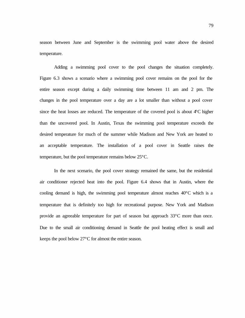
79

season between June and September is the swimming pool water above the desired

temperature.

Adding a swimming pool cover to the pool changes the situation completely.

Figure 6.3 shows a scenario where a swimming pool cover remains on the pool for the

entire season except during a daily swimming time between 11 am and 2 pm. The

changes in the pool temperature over a day are a lot smaller than without a pool cover

since the heat losses are reduced. The temperature of the covered pool is about 4°C higher

than the uncovered pool. In Austin, Texas the swimming pool temperature exceeds the

desired temperature for much of the summer while Madison and New York are heated to

an acceptable temperature. The installation of a pool cover in Seattle raises the

temperature, but the pool temperature remains below 25°C.

In the next scenario, the pool cover strategy remained the same, but the residential

air conditioner rejected heat into the pool. Figure 6.4 shows that in Austin, where the

cooling demand is high, the swimming pool temperature almost reaches 40°C which is a

temperature that is definitely too high for recreational purpose. New York and Madison

provide an agreeable temperature for part of season but approach 33°C more than once.

Due to the small air conditioning demand in Seattle the pool heating effect is small and

keeps the pool below 27°C for almost the entire season.

80

Unheated and Uncovered Swimming Pool for Different Locations

0

5

10

15

20

25

30

35

40

2880 3610 4340 5070 5800 6530

Time [Hrs]

Sw

imm

ing

Po

ol T

em

pera

ture

[C

]

Austin

Madison

New York

Seattle

Comfort Pool Temperature


Figure 6.2 Swimming pool temperature for an uncovered and unheated pool

Unheated Pool for Different Locations

0

5

10

15

20

25

30

35

40

2880 3610 4340 5070 5800 6530

Time [Hrs]

Sw

imm

ing

Po

ol T

em

pera

ture

[C

]

Austin

Madison

New York

Seattle


Uncovered 11:00-14:00


Figure 6.3 Pool temperature for an unheated and uncovered pool between 11am and 2pm

81

Heat Pump Heated Pool for Different Locations

0

5

10

15

20

25

30

35

40

2880 3610 4340 5070 5800 6530

Time [Hrs]

Sw

imm

ing

Po

ol T

em

pera

ture

[C

]

Austin

Madison

New York

Seattle


Uncovered 11:00-14:00


Figure 6.4 Pool temperature for a heated and part time covered pool

Heat Pump Heated Swimming Pool for Different Locations

0

5

10

15

20

25

30

35

40

2880 3610 4340 5070 5800 6530

Time [Hrs]

Sw

imm

ing

Po

ol T

em

pera

ture

[C

]

Austin

Madison

New York

Seattle


Cover controlled


Figure 6.5 Automatic pool cover controlled swimming pool temperature

82

Applying the advanced pool cover control strategy where the swimming pool

remains uncovered if the temperature exceeds 26°C Figure 6.5 shows that a substantial

cooling effect can be achieved. Again, the heat removal from the building is added to the

pool. The extreme pool temperatures for Austin of the last example can be reduced to a

maximum of 30°C. Madison and New York can be maintained oscillating around the

desired temperature. Since the control strategy only effects high pool temperatures the

results for Seattle are not affected. In this case a swimming pool gas heater would be

needed.

6.2.4. Summary

It has been shown that a swimming pool cover influences the swimming pool

temperature significantly. An overview of average swimming pool temperatures is

provided in Table 6.1. Adding a cover to the swimming pool raises the pool temperature

about 4°C. Combining a pool cover with the swimming pool air conditioner increases the

temperature another 4°C. To avoid overheating, the automatic pool cover controller

adjusts the pool temperature again to a lower temperature level.

Average Swimming Pool Temperature

Cities Uncovered Unheated

Uncovered 11:00 – 14:00 Unheated

Uncovered 11:00-14:00 Heat Pump heated

Automatic Pool Cover Heat Pump heated

Austin 26.0 29.8 34.0 27.5

Madison 19.6 23.2 26.0 24.0

New York 20.6 24.7 27.7 24.9

Seattle 16.5 20.4 22.7 22.5

Table 6.1 Comparison of average swimming pool temperatures for different locations.

83

Note that Table 6.1 shows seasonal averages that can be lower than the

comfortable temperatures. However, the cooling effect results in a higher pool water loss

that has to be equalized from time to time. The water loss has been investigated in Section

6.4.

6.3 Benefits for the Customer

In this section the operation costs for both conventional air conditioning and gas

heating and the combined house cooling and pool heating are presented. The separate air

conditioning and gas pool heating is referred to as conventional system, while the

combined swimming pool heater and air conditioner will be called the swimming pool air

conditioner (SPAC).

6.3.1. System Control Strategies

To compare the two systems on a fair basis the following control strategy has been

developed. First, for swimming pool temperatures less than 25°C a gas pool heater adds

heat to the pool. The gas heater maintains this temperature for both system

configurations. Since the swimming pool air conditioner rejects heat whenever a cooling

demand exits, the additional heat from the gas pool heater will be less.

If the swimming pool temperature exceeds 26°C the automatic swimming pool

cover controller opens the pool and regulates the temperature by evaporation. The

building temperature is controlled during the entire season so that heat is removed by the

air conditioner whenever the temperature exceeds 25°C. One possible arrangement of the

84

system components modeled in the SPAC simulation program are shown in Figure 6.6

where the air conditioner is in water-cooling mode and the gas furnace joins to maintain

the desired swimming pool temperature.

Gas Furnace AC

Figure 6.6 The Swimming Pool Air Conditioner Configuration

Based on these control mechanisms the SPAC simulation has been modified to

run for different locations in the United States. Ten Cities have been chosen for an

economic analysis and are shown in Figure 6.7. Different climates were examined for

pool behavior and heating requirements to observe the impact on the economic analysis

and narrow down regions where the swimming pool air conditioner performs best.

85

BaltimoreNew York

$Miami

$

$

$Austin

$

Atlanta

$Madison

$St. Louis

$Phoenix$

Los Angeles

$Seattle

Figure 6.7 Cities for economic analysis

6.3.2. Seasonal Operation Cost

For each location the monthly energy requirement has been calculated for a

conventional air conditioner with a gas pool heater and for a swimming pool air

conditioner with a gas pool heater. The simulation was started in the beginning of May

and continued until the beginning of October. For this period the swimming pool

temperature was maintained to be at least 25°C using the gas pool heater when necessary.

For some locations the pool might exceed the desired temperature resulting from solar

gains and heat removed from the building that cannot be controlled by the cover

controller. Table 6.2 shows that the maximum pool temperature stays below 32°C even

for warm climates like Miami or Austin.

86

Seasonal Savings [$]

AC GPH SPAC GPHAtlanta GA 26.2 29.9 202 3 26.6 31.3 154 1 50Austin TX 27.2 32.0 279 0 27.8 33.6 203 0 76Baltimore MD 25.8 29.2 171 46 26.2 30.2 133 24 60Los Angeles CA 25.7 27.6 182 31 26.0 28.4 147 11 56Madison WI 25.4 28.1 136 150 25.7 29.0 105 105 77Miami FL 27.3 31.3 251 0 28.0 32.7 186 0 65New York NY 25.6 28.6 154 75 25.9 29.6 120 44 65Phoenix AZ 26.7 30.5 394 0 27.4 32.2 268 0 126Seattle WA 25.1 26.8 113 224 25.4 27.4 95 154 88St.Louis MO 26.1 29.8 209 16 26.5 31.2 158 8 59

City (May 1st -

October 1st)

Conventional System

Average Pool Temp [C]

Max Pool Temp [C]

Cost [$]Average

Pool Temp [C]

Max Pool Temp [C]

Cost [$]

SPAC System

Control StrategiesGas Pool Heater(GPH): Cover opens if Tpool > 26 C , Else the pool is open between 11am - 2 pmHeater activates if Tpool < 25 CSwimming Pool Air Conditioner(SPAC):Cover opens if Tpool > 26 C , Else the pool is open between 11am - 2 pm

Economic AnalysisGas : 0.02 $/kWhElectricity: 0.075 $/kWh

Table 6.2 Temperatures and Operation Cost for the examined systems. GPH is a Gas Pool

Heater, AC is a Conventional Air Conditioner and SPAC is a Swimming Pool Air

Conditioner.

The table also shows the component operation cost for cooling and heating for

both, the conventional and the SPAC system. Figure 6.8 visualizes this result by showing

columns for each system and location. The left column represents the conventional

system, where the air conditioning operation cost is added to the seasonal pool heating

cost. The right column shows the cost for the SPAC system and if additional pool heating

is necessary the cost for natural gas. The cities are ordered by decreasing cooling demand.

87

Seasonal Operating Cost For Pool Heating Systems

0

100

200

300

400

500

600

Phoenix Austin Miami Atlanta St.Louis LosAngeles

Baltimore NewYork

Madison Seattle

Sea

son

al C

ost

[U

S$]

Conventional Air Conditioner

Gas Pool Heater

Swimming Pool Air Conditioner

Season : May 1st - October 1stbased on 0.075 $/kWh Electricity , 0.02 $/kWh Natural Gas

Pool Area = 55 m2

Figure 6.8 Economic analysis for locations in different climates in the United States. For each

City the left column shows the conventional house cooling and heating, while the

right includes the swimming pool air conditioner plus additional pool heating cost.

In Phoenix, for example, no gas heating is necessary for either the conventional or

SPAC system to maintain a comfortable swimming pool temperature. But, due to the

better performance of a water-cooled air conditioner the operation cost is lower. By

comparing the swimming pool temperatures for both systems, Table 6.2 clarifies that

there is no major change in swimming comfort due to the heat rejection to the pool. The

maximum temperature increases only about 1.5°C, while the average only changes about

1°C.

88

0

50

100

150

200

250

300

350

400

450


Baltimore New York Madison Seattle

Ele

ctri

city

Cos

t [U

S$]

AC

SPAC

Pool Area = 55 m2

Figure 6.9 Electricity Cost for house cooling for a season between May 1st to October 1st based

on 0.075 $/kWh

0

50

100

150

200

250

300

350

400

450



Nat

ural

Gas

Cos

t [U

S$]

AC

SPAC

Pool Area = 55 m2

Figure 6.10 Natural Gas Cost for swimming pool heating between May 1st to October 1st based on

0.02 $/kWh

89

With decreasing ambient temperatures, the cooling demand for a building

decreases. Accordingly, the rejected heat to the swimming pool is less and pool heating

becomes more important. Also, due to the lower ambient temperatures in cooler climates

the general need for gas pool heating increases. Thus, the electricity cost decreases while

the cost for natural gas increases.

For a better comparison, Figure 6.9 and Figure 6.10 show the expenses for

electricity and natural gas separated in two charts. The left column for each city

represents the conventional system configuration and the right column the swimming

pool air conditioner.

The cooling demand is the major impact on the electricity cost. Thus, the warmer

the ambient conditions at the specific location the higher the required energy to maintain

the building temperature. However, there is still an advantage of the swimming pool air

conditioner because of its better general performance due to the lower cooling fluid of the

condenser.

Based on the natural gas consumption two city groups can be identified. The first

group includes cities where gas pool heating is not necessary at all. Phoenix, Austin,

Miami and Atlanta can be counted to this group. The second group consists of cities that

need gas pool heating for both system configurations to maintain the desired swimming

pool temperature as seen in New York, Seattle, Madison, St. Louis and Baltimore. A few

locations cannot be assigned to one of the groups easily. Los Angeles for example has

almost no heating demand for the swimming pool air conditioner and could be counted to

the second group.

90

6.3.3. Seasonal Savings for Different Locations

Compared to the conventional system, the customer can save on seasonal

expenses using the swimming pool air conditioner. Because of the better performance, the

SPAC saves electricity. Figure 6.11 shows the electricity savings as a function of the

cooling demand at different locations. The higher the expenses for the conventional air

conditioner, the higher the seasonal savings.

Because the SPAC rejects the heat to the pool that is usually released to the

ambient, the cost for heating is reduced. Figure 6.12 shows the seasonal gas savings.

0

20

40

60

80

100

120

140



Sea

sona

l Ele

ctri

city

Sav

ings

[US

$]

Pool Area = 55 m2

Figure 6.11 Electricity savings for SPAC compared to a conventional system for a season from

May 1st to October 1st based on 0.075 $/kWh

91

0

20

40

60

80

100

120

140

160



Sea

sona

l Nat

ural

Gas

Sav

ings

[US

$]

Pool Area = 55 m2

Figure 6.12 Natural Gas Savings for SPAC compared to a conventional system for a season

from May 1st to October 1st based on 0.02 $/kWh

6.3.4. Impact of Different Swimming Pool Sizes

In addition to the swimming pool investigated above, the impact of varying pool

sizes is examined. Starting with the base case pool size of 55 m2 a smaller swimming pool

(27.5 m2) and a larger pool (110 m2) are investigated. Figure 6.13 and Figure 6.14 show

the effect on the economic analysis. Since the building and the air conditioning system

remained the same, the amount of rejected heat is constant for the three cases.

Independent of the pool sizes the pool conditions can be adjusted without supplemental

heat from a gas pool heater in Phoenix, Austin, Miami and Atlanta. For locations that

require pool heating to maintain the swimming pool at the comfortable swimming pool

temperature of 27 °C the natural gas consumption increases for increasing pool area.

92


0

100

200

300

400

500

600


Baltimore NewYork

Madison Seattle

Sea

son

al C

ost

[U

S$]


Gas Pool Heater



Pool Area = 27.5 m2

Figure 6.13 Economic analysis for locations in different climates in the United States for a 27.5

m2 pool.


0

100

200

300

400

500

600


Baltimore NewYork

Madison Seattle

Sea

sona

l Cos

t [U

S$]


Gas Pool Heater



Pool Area = 110 m2

Figure 6.14 Economic analysis for locations in different climates in the United States for a 110 m2

pool.

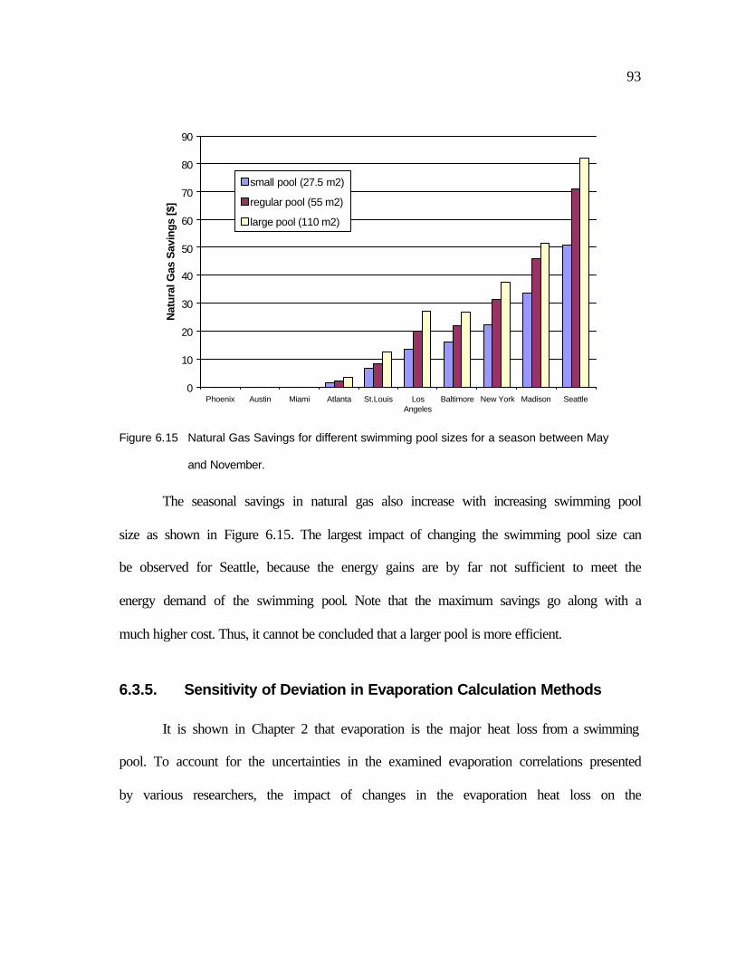
93

0

10

20

30

40

50

60

70

80

90



Nat

ural

Gas

Sav

ings

[$]

small pool (27.5 m2)

regular pool (55 m2)

large pool (110 m2)

Figure 6.15 Natural Gas Savings for different swimming pool sizes for a season between May

and November.

The seasonal savings in natural gas also increase with increasing swimming pool

size as shown in Figure 6.15. The largest impact of changing the swimming pool size can

be observed for Seattle, because the energy gains are by far not sufficient to meet the

energy demand of the swimming pool. Note that the maximum savings go along with a

much higher cost. Thus, it cannot be concluded that a larger pool is more efficient.

6.3.5. Sensitivity of Deviation in Evaporation Calculation Methods

It is shown in Chapter 2 that evaporation is the major heat loss from a swimming

pool. To account for the uncertainties in the examined evaporation correlations presented

by various researchers, the impact of changes in the evaporation heat loss on the

94

simulation results were investigated. As can be seen in Figure 6.16 an uncertainty of

±10% results in a change in the natural gas cost of ±10%.

Sensitivity for Deviation in Evaporation

-70

-60

-50-40

-30

-20-10

010

20

3040

50

6070

40 50 60 70 80 90 100 110 120 130 140 150 160

Frac

tiona

l Nat

ural

Gas

Cos

t [%

]

SPAC

Conventional

Fractional Evaporation [%]

Figure 6.16 Impact of uncertainties in evaporation calculation methods on the natural gas cost for

the SPAC and conventional systems.

6.3.6. SPAC Equipment Cost

Further investigations have been made to examine the extra budget that is

available to manufacture a swimming pool air conditioner. The fact that SPAC is more

efficient than a conventional air conditioner provides the advantage for the manufacturer

to make it more expensive. The maximum possible additional product cost is reached

when the life-cycle cost of the SPAC is the same as the conventional system. Duffie and

Beckman (1991) provide a method to calculate the life cycle cost for a system. The life

cycle cost (LCC) is the sum of all the costs associated with an energy delivery system

95

over its lifetime or over a selected period of analysis, in today’s dollars, and takes into

account the time value of money. Life cycle savings is defined as the difference between

the life cycle costs of a conventional air conditioner and pool heating system and the life

cycle cost for the swimming pool air conditioner system. Duffie and Beckman (1991)

have shown how all economic parameter can be cast in only two parameters, P1 and P2.

Thus, the life cycle cost for the conventional system and the SPAC can be written as

( ) conveqcomvgconveConv CPCCPLCC ,2,,1 ⋅++= ( 6.1 )

( ) SPACeqSPACgSPACeSPAC CPCCPLCC ,2,,1 ⋅++= ( 6.2 )

Where Ce is the electricity cost for the first year of analysis, Cg the natural gas cost

for the first year of the analysis and Ceq the equipment cost of the system.

The difference of equation ( 6.1 ) and equation ( 6.2 ) results in the an expression

for the life cycle savings of the SPAC system. For a break-even calculation the life cycle

savings are zero.

( ) 021 =∆⋅−∆+∆= eqge CPCCPLCS ( 6.3 )

Since the savings ∆Ce and ∆Cg are known, equation ( 6.3 ) can be solved for the

difference in equipment cost ∆Ceq.

( )geeq CCPP

C ∆+∆=∆2

1 ( 6.4 )

The difference of the equipment cost is the maximum money that can be charged

by the manufacturer for a swimming pool air conditioner that has the same life cycle cost

as a conventional air conditioner plus pool heating system.

96

0

200

400

600

800

1000

1200

1400



Incr

emen

tal E

quip

men

t Cos

t [U

S$]

Pool Area = 55 m2

Figure 6.17 Incremental equipment cost for a SPAC system compared to a conventional system

because of better performance. Time period: May 1st to October 1st.

Because the detailed system component cost and various economic parameters

especially for the swimming pool air conditioner, are not available an approximate value

for the ratio of P1/P2 can be obtained by the following assumptions: If the inflation rate of

fuel (electricity and gas) is of the order of the general inflation rate, then P1 is of the order

of the period of the economic analysis. P2 is unity if the system is paid for in cash.

Therefore, the ratio of P1/P2 equals the period of the economic analysis. For the present

work, a period of ten years has been chosen. Figure 6.17 shows the result of this

approach. The allowable costs are between about $600 and $1000 for most locations, with

higher values in the very hot climates of Austin and Phoenix. A minimum is found for

Atlanta, which can be taken as additional budget that is available to finance the redesign

of the air conditioner.

97

6.3.7. Air Conditioner Power Demand

An interesting aspect for power plant companies is the power demand for air

conditioners. Since air conditioning consumes power mostly during the daytime where

the energy demand is high, a reduction would be beneficed to the power company. Figure

6.18 shows a comparison of the maximum power demand for a conventional air

conditioner that uses air as cooling fluid to a swimming pool air conditioner. The air-

cooled power demand is almost uniformly at about 6 kW. The SPAC system energy

demand is about 5 kW, which results in a demand saving of 1 kW compared to

conventional air conditioning systems. Applying the swimming pool air conditioner this

demand can be reduce by about 20%.

Air Conditioning Power Demand

0

1

2

3

4

5

6

7

8

9

10

Atlanta Austin Baltimore LosAngeles

Madison Miami New York Phoenix Seattle St.Louis

Pow

er D

eman

d [k

W]

air-cooled

water-cooled

Figure 6.18 Power demand comparison for air conditioner systems.

98

6.3.8. Summary

In this section it has been shown that water-cooled air conditioners that reject heat

to a swimming pool work more efficiently than conventional air-cooled air conditioners.

In some climates additional swimming pool heating is not necessary with the proposed

swimming pool air conditioner because the heating demand is accomplished by the

rejected heat. In warmer regions where swimming pool heating is not necessary at all, the

improved performance of a water-cooled air conditioner reduces the operation cost. For

most locations in the United States additional pool heating is necessary. Despite this fact,

the SPAC system still performs better than conventional methods according to the heat

rejection to the pool.

In conclusion, the proposed swimming pool air conditioner is shown to perform

better than conventional solutions. The amount of savings is dependent of the location of

the customer but saves at least $60 per season.

6.4 Swimming Pool Water Level Calculations

Every water body has water losses due to evaporation. Thermodynamically, the

evaporation heat loss is proportional to the amount of water that is lost by the pool:

evapevap hVQ ∆⋅⋅ρ=••

( 6.5 )

Where evapQ•

is the evaporation energy, ρ is the density of water, evaph∆ is the

enthalpy of evaporation and wV•

is the volume of evaporated water, e.g. the water loss per

99

unit time [m3/hr]. The enthalpy of evaporation is a function of the swimming pool

temperature and can be linearly approximated by

poolevap Th ⋅−=∆ 659.6652.1602 . ( 6.6 )

Where the Tpool is the pool temperature is in degree Celsius.

The water loss can be calculated from equation ( 6.6 ) by knowing the amount of

energy that is evaporated from the swimming pool surface.

Information for the monthly average precipitation has been obtained from the

annual weather summary for Madison, WI (NCDC (1998)). The amount of rain per

square meter has been multiplied by the total pool area to calculate the total amount of

water added to the swimming pool due to precipitation.

Applying the water loss calculation to the SPAC simulation for Madison over a

season from May to October using the automatic cover control and heat rejection to the

pool results in a water loss of 27.4 m3. This evaporation about one third of the total pool

volume (82.5 m3). Precipitation adds 24.6 m3 water to the pool. Therefore, in Madison

almost no water has to be replaced due to evaporation. This can only be an approximation

since other effects influence the water loss of a swimming pool.

101

Chapter 7 Conclusions and Recommendations

The goal of this project was to investigate the performance of an air conditioner

that rejects energy to a swimming pool instead of to the ambient air. Swimming pools and

air conditioners have been examined separately in Chapter 2 and 3. Both components are

available as TRNSYS types that were implemented in the swimming pool air conditioner

simulation (SPAC).

Chapter 6 concludes that it is generally possible to heat a pool and to keep the

building at a comfortable temperature using a swimming pool air conditioner system. In

some climates a swimming pool heater is not necessary because the heat rejected by the

swimming pool air conditioner alone maintains a comfortable pool temperature. Due to

the fact that water is used as the cooling fluid, a swimming pool air conditioner performs

better than conventional air conditioners. Thus, the purchased energy for pool heating and

house cooling can be reduced. The manufacturer can most likely include higher

manufacturing costs into the first cost while the customer enjoys the benefit of lower life

cycle cost.

The swimming pool air conditioner simulation program provides a research tool

for swimming pool manufactures and customers. The program is suitable for directly

estimating the economic impact of different scenarios. The SPAC program can be used to

investigate various configurations of a swimming pool, a gas pool heater, an air

102

conditioner and a building for different time periods and locations. SPAC provides

information on the component performance as well as hourly information on system

parameters. The cost advantage of one alternative over the other can be determined. The

present system can be analyzed and the impact of an additional device studied before an

investment is made.

Compared to a conventional system, the customer can save on seasonal expenses

using the swimming pool air conditioner. Because of the better performance, the SPAC

saves electricity. The seasonal electricity savings vary for different climates but are

between $40 and $80 for most locations. Because the SPAC rejects the heat to the pool

that is usually released to the ambient, the cost for swimming pool heating is reduced.

The customer can save about $40 on natural gas by using the SPAC system.

The allowable incremental equipment costs for a swimming pool heater system

compared to a conventional system configuration, are between about $600 and $1000 for

most locations, with higher values in the very hot climates of Austin and Phoenix. The

SPAC system energy demand is about 5 kW, which results in a demand saving of 1 kW

compared to conventional air conditioning systems.

The cooling requirements of a building and the pool heating demand are

dependent on the climate. In warmer climates a swimming pool air conditioner rejects

more heat to the swimming pool than in moderate climates. Thus, overheating is possible.

In this work the swimming pool temperature was reduced by removing a pool cover from

the surface to allow evaporation. An object of further investigation could be an air

conditioning device that hosts both air and water-cooling. After determining if the

103

swimming pool requires heating a control mechanism would then reject the heat either to

the pool or the environment.

The mathematical descriptions of the modeled components are considered to

produce results that are accurate enough for the task of this work. However, as with all

theoretical studies, simulations can only approximate reality. Thus, for further

investigation a swimming pool air conditioner has to be designed and manufactured to

obtain measurements that can verify the results of this research.

105

References

ASHRAE (1982). ASHRAE Handbook - Applications. Atlanta, GA, American Society

of Heating, Refrigeration and Air Conditioning.

ASHRAE (1991). ASHRAE Handbook - 1991 HVAC Applications. Atlanta, American

Society of Heating Refrigeration and Air Conditiong Engineers, Inc.

ASHRAE (1997). ASHRAE Handbook - 1997 Fundamentals. Atlanta, American Society

of Heating Refrigeration and Air Conditiong Engineers, Inc.

ASHRAE (1999). ASHRAE Handbook - 1999 Applications. Atlanta, GA, American

Society of Heaeting, Refrigerating and Air-Conditioning Engineers, Inc.

Auer, T. (1996). TRNSYS-TYPE 144: Bilanzierung eines Hallen-bzw.

Freischwimmbeckens. Stuttgart, TRANSSOLAR.

Beckman, W. A., S. A. Klein, et al. (1977). Solar Heating Design by the F-Chart Method.

Madison, WI, Solar Energy Laboratory, University of Wisconsin, Madison.

Behrdahl, P., D. Grether, et al. (1978). “California Solar Data Manual.” .

Bowen, I. S. (1926). “The ratio of heat Losses by Conduction and by Evaporation from

any Water.” Physical Review 27: 787-799.

Brunt, D. (1938). “Notes on Radiation in the Atmosphere.” Quaterly Journal of the Royal

Meteorollogy Society 58: 389-420.

Carrier, W. H. (1918). “The Temperature of Evaporation.” ASHVE Transactions 24: 25-

50.

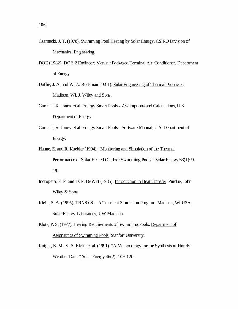
106

Czarnecki, J. T. (1978). Swimming Pool Heating by Solar Energy, CSIRO Division of

Mechanical Engineering.

DOE (1982). DOE-2 Endineers Manual: Packaged Terminal Air-Conditioner, Department

of Energy.

Duffie, J. A. and W. A. Beckman (1991). Solar Engineering of Thermal Processes.

Madison, WI, J. Wiley and Sons.

Gunn, J., R. Jones, et al. Energy Smart Pools - Assumptions and Calculations, U.S

Department of Energy.

Gunn, J., R. Jones, et al. Energy Smart Pools - Software Manual, U.S. Department of

Energy.

Hahne, E. and R. Kuebler (1994). “Monitoring and Simulation of the Thermal

Performance of Solar Heated Outdoor Swimming Pools.” Solar Energy 53(1): 9-

19.

Incropera, F. P. and D. P. DeWitt (1985). Introduction to Heat Transfer. Purdue, John

Wiley & Sons.

Klein, S. A. (1996). TRNSYS - A Transient Simulation Program. Madison, WI USA,

Solar Energy Laboratory, UW Madison.

Klotz, P. S. (1977). Heating Requirements of Swimming Pools. Department of

Aeronautics of Swimming Pools, Stanfort University.

Knight, K. M., S. A. Klein, et al. (1991). “A Methodology for the Synthesis of Hourly

Weather Data.” Solar Energy 46(2): 109-120.

107

Martin, M. and D. R. F. Behrdahl (1984). “Characteristics of Infrared Sky Radiation in

the United States.” Solar Energy 33(3/4): 321-336.

NCDC (1998). Annual Summary with Comparative Data. Madison, WI, National Climate

Data Center.

NREL (1995). User's Manual for TMY2s. Colorado, National Renewable Energy

Laboratory (NREL).

Richter, D. (1969). Ein Beitrag zur bestimming der Verdunstung von freien

Wasserflaechen. Berlin, Meteorologischer Dienst der DDR.

Richter, D. (1979). Temperatur- und Waermehaushalt des thermisch belasteten Stechlin-

und Nehmitzsees. Berlin, Akademie Verlag.

Roberson, J. A. and C. T. Crowe (1985). Engineering Fluid Mechanics, Houghton &

Mifflin.

Ryan, P. J. and D. R. F. Harleman (1973). An Analytical and Experimental Study of

Transient Cooling Pond Behavior, Ralph M. Parson Laboratory for Water

Rescources and Hydrodynamics.

Smith, C., D. Jones, et al. (1993). Energy Requirements and Potential Savings for Heated

Indoor Swimming Pools. Engineers Transaction. Denver, CO, American Society

of Heating, Refrigeration and Air Conditioning. Symposia DE-93-12-3.

Smith, C. C., G. Loef, et al. (1994). “Measurement and Analysis of Evaporation From an

Inactive Outdoor Swimming Pool.” Solar Energy 53(1): 3-7.

Transsolar (1997). PREBID for WINDOWS. Stuttgart, TRANSSOLAR.

108

Wei, J., H. Sigworth, et al. (1979). A Computer Program for Evaluating Swimming Pool

Heat Conservation. Berkeley, CA 94720, University of California.

Wei, J., H. Sigworth, et al. (1979). Reducing Swimming Pool Heating Cost: Comparison

of Pool Covers, Solar Collectors and Other Options. Berkeley, CA., 94720,

Energy and Environment Division

109

Appendix A Description of TRNSYS Type 144

A.1 General Description

TRNSYS TYPE 144, developed at TRANSSOLAR in Germany, simulates both indoor

and outdoor swimming pools. The inputs and outputs as well as the parameters () are

described in this section.

Figure A.1 Input and output for TYPE 144

A.2 Description of the Inputs

To simulate an outdoor or indoor swimming pool the following inputs are used:

Input no. Symbol Description Unit 1 TAmb ambient air temperature [°C]

1: TP,0

2: Atot

7: λcov

8: δcov 3: V 4: modeN

5: εcov

6: αcov 9: hM,0 10: Sfac

Parameter

TYPE 144 Swimming Pool Simulation

TAmb ϕAmb ωAmb EGlob,H TSky TWall QSol mode1 mtap Ttap topen tclose Nmax fcov min Tin

13 1 2 3 4 5 7 6 8 9 10 11 12 14 15 16

Input

TP mevap Qevap Qconv Qrad Qtap QSol Qin DE TP min

1 2 3 4 5 7 6 8 9 10 11

Output

110

2 ϕAmb relative humidity of ambient air [%] 3 ωAmb velocity of ambient air [m/s] 4 EGlob,H global radiation on horizontal surface [kJ/h-m2] 5 TSky sky temperature [°C] 6 TWall temperature of pool walls [°C] 7 QSol window radiative energy gains [kJ/h] 8 Mode1 water surface activity [-] 9 mtap mass flow rate of tap water [kg/h] 10 Ttap temperature of tap water [°C] 11 Topen pool opening time [-] 12 Tclose pool closing time [-] 13 Nmax daily maximum number of people in the pool [-] 14 fcov fractional coverage of water surface [-] 15 min mass rate of incoming warm water [kg/h] 16 Tin temperature of incoming warm water [°C] 1. Ambient Air Temperature (TAmb)

For an outdoor pool this temperature should be the outside air temperature. For an indoor

pool room temperature should be used.

2. Relative Humidity of Ambient Air (ϕAmb)

Depending upon the ambient air temperature chosen above ,the relative humidity is taken

to be the relative humidity of either the outdoor or the indoor air.

3. Velocity of Ambient Air (ωAmb)

This input is used only for an outdoor swimming pool calculation. Because the wind

speed is a function of the height above ground and the microclimate around the pool, two

additional parameters have been added to determine this value. (See Parameters)

4. Global Radiation on Horizontal Surface (EGlob,H)

To calculate the radiation heat gains to an outdoor pool the radiation on a horizontal

surface is needed.

5. Sky Temperature (TSky)

111

To calculate the exchange of long wave radiation a sky temperature is necessary. This can

be found using TYPE 69.

6. Temperature of Pool Walls (TWall)

To calculate the exchange of long wave radiation for an indoor pool an average wall

temperature of the pool is needed.

7. Window Radiation Gains (QSol)

Only of use for the calculation of the energy gains of an indoor pool. The window

radiation gains are energy inputs to the pool due to sunlight shining through windows.

This input can be calculated by TYPE 56, output 21.

8. Water Surface Activity (mode1)

The motion of the water surface has a strong influence on evaporation and convection.

Therefore a switch is used to set one of the following modes:

mode1 = 0 quiet water surface mode1 = 1 slight surface motion (private pool) mode1 = 2 slight surface motion (public pool) mode1 = 3 moderate surface motion (recreational pool) mode1 = 4 intense surface motion (wave pool) mode1 = -1 activity function

The activity function (mode1 = -1) computes a parabola between opening and closing time

of the pool. The maximum is located in the middle. Therefore it is necessary to use inputs

11, 12 and 13.

9. Mass Flow Rate of Tap Water (mtap)

Input 9 describes only the water rejection for hygienic purposes. The loss of water due to

evaporation is compensated automatically.

10. Temperature of Tap Water (Ttap)

112

Temperature of incoming tap water (input 9). Tap water flows for both hygienic and

evaporative compensation are assumed to have the same temperature.

11. Pool Opening Time (topen)

The time of day (0-24) when pool usage begins. (needed for the calculation of the activity

function.)

12. Pool Closing Time (tclose)

(see input 11 and 8)

13. Daily Maximum Number of People in the Pool (Nmax)

Input 13 is also used to calculate the activity function (input 8). The input is the daily

maximum number of people in the pool. In a pool with an area of 100m2 and 100 people a

day for example, the activity function has a maximum of 4 compared to an unused pool.

14. Fractional Coverage of Water Surface (fcov)

The percentage of time pool surface is covered (fcov = 0..1)

15. Mass Flow Rate of Incoming Warm Water (min)

Mass flowrate entering pool from the heating system

16. Temperature of Incoming Warm Water (Tin)

Temperature of water entering the pool from the heating system.

A.3 Description of Parameters

To simulate an outdoor or indoor swimming pool the following parameters are used:

Input no. Symbol Description Unit 1 TP,0 initial temperature of pool water [°C]

113

2 Atot total surface area of pool [m2] 3 V volume of pool water [m3] 4 ModeN switch between outdoor and indoor pool [-] 5 εcov emissivity of pool cover [-] 6 αcov Absorption of cover [-] 7 λcov heat transfer coefficient of cover [kJ/h-m-K] 8 δcov thickness of cover [m] 9 hM,0 height of wind measurement [m] 10 Sfac Shelter factor [-] 1. Initial Temperature of Pool Water (TP,0)

Temperature of the pool at the time when simulation starts.

2. Total Surface Area of the Pool (Atot)

Surface Area of the swimming pool including the spillway.

3. Pool Water Volume (V)

4. Switch between outdoor and indoor pool (modeN)

The parameter modeN switches between the calculation of an indoor and an outdoor

swimming pool:

modeN = 0 Indoor Pool modeN = 1 Outdoor Pool

5. Emissivity of Pool Cover (εcov)

6. Absorption of Pool Cover (αcov)

7. Heat Transfer Coefficient of Cover (λcov)

8. Thickness of Cover (δcov)

114

9. Height of Wind Measurement (hM,0)

(See parameter 10)

10. Shelter Factor (Sfac)

The heat loss of an outdoor swimming pool depends strongly on the wind speed. In this

program a wind speed measurement height of 3m above ground is assumed. Because this

is not necessarily the height at which the wind speed was actually measured, a correction

term is included. The correction term depends on the shelter of the pool due to the

surroundings. Figure A.2 shows an example where the wind velocity measured is 5m/s at

a height of 10m.

Figure A.2 The height as a function of wind speed. Measured wind velocity at the airport: 5 m/s at

a height of 10m

The following relation is used to compute the modified wind velocities:

0

1

2

3

4

5

6

7

8

9

10

0 1 2 3 4 5

Wind Speed [m/s]

Hei

gh

t of M

easu

rem

ent [

m]

Sfac = 2Sfac = 4Sfac = 6Sfac = 8Sfac = 10

Height of Measurement

Height used in Calculation

115

Sfacrelairport h

hvv

1

0

⋅=

Sfac = 2 strong shelter

Sfac = 2-4 normal shelter

Sfac = 3-6 wooded area

Sfac = 6-8 unsheltered

Sfac = 8-10 open water

hrel = height of wind measurement

h0 = 3 m

A.4 Description of the Outputs

Input no. Symbol Description Unit 1 TP pool water temperature [°C] 2 mevap mass flow rate due to evaporation [kg/h] 3 Qevap evaporation heat flux [kJ/h] 4 Qconv convection heat flux [kJ/h] 5 Qrad radiation heat flux [kJ/h] 6 Qtap heat loss due to tap water [kJ/h] 7 QSol solar heat gain [kJ/h] 8 Qin added heat flux [kJ/h] 9 DE energy stored in the pool [kJ] 10 TP pool water temperature [°C] 11 min mass rate of incoming warm water [kg/h]

The component outputs are basically self-explanatory.

117

Appendix B SPAC Output Files

This section includes the description of the output of the swimming pool air

conditioner simulation (SPAC). The output files can be found in C:\SPAC\.

B.1 General System Information

The file spac.ou1 provides general system information on an hourly basis.

Output Parameter Description Time Hour of Year of Simulation Tamb Ambient Dry Bulp Temperature [C] Tpool Swimming Pool Temperature [C] Tbuild Building Temperature [C] Qhouse Building Cooling Demand [kJ/hr] Qcond Air Conditioner Energy Output [kJ/hr] Power Air Conditioner Power Consumption [kJ/hr]

B.2 Swimming Pool Information

Output file spac.ou2 provides hourly values for the swimming pool

Output Parameter Description Time Hour of Year of Simulation Qevap Pool Evaporation Heat Loss [kJ/hr] Qconv Pool Convection Heat Loss [kJ/hr] Qrad Pool Radiation Heat Loss [kJ/hr] Qsol Pool Solar Gains [kJ/hr] Qheater Heat added to the pool by pool heater [kJ/hr] Qcooler Energy removed from the pool by the cooler [kJ/hr]

118

B.3 Weather Information

Weather information for the desired location is available in output file spac.ou3.

Output Parameter Description Time Hour of Year of Simulation Ibeam Direct Normal Solar Radiation [kJ/hr] Iglob Global Solar Radiation on a horizontal surface [kJ/hr] Tamb Ambient Temperature [C] Humrat Humidity Ratio WindVel Wind Velocity [m/s]

B.4 Air Conditioner Information

Output file spac.ou4 provides hourly information on air conditioner performance.

Output Parameter Description Time Hour of Year of Simulation Tc,in,w Condenser Inlet Temperature (Pool Water) [C] COPwater Coefficient of Performance for Pool Water [-] Wwater Air Conditioner Power for Water-Cooling[kW] Qcond,w Condenser Energy for Water-Cooling [kJ/hr] Tc,in,a Condenser Inlet Temperature (Ambient Air) [C] COPair Coefficient of Performance for Ambient Air [-] Wair Air Conditioner Power for Air-Cooling[kW] Qcond,a Condenser Energy for Air-Cooling [kJ/hr]

B.5 Economics Information

Monthly information of the economic analysis is available in output file *.ou5.

Output Parameter Description Time Hour of Year of Month Costwater Cost for Water-Cooled Air Conditioning [$/month] Costair Cost for Air-Cooled Air Conditioning [$/month] Costgas Cost for Gas Pool Heating [$/month]

119

Costpumpheat Cost for Water Pump for Pool Heating [$/month] Costcool Cost for Water Cooling [$/month] Costpumpcool Cost for Water Pump for Pool Cooling [$/month]

B.6 Power Consumption Information

Monthly information of the power consumption of different devices is available in

output file spac.ou6.

Output Parameter Description Time Hour of Year of Month Pac,air Air-Cooled AC Power Consumption [kJ/month] Pac,water Water-Cooled AC Power Consumption [kJ/month] Pheat Power Consumption of Gas Pool Heater [kJ/month] Pcool Power Consumption of Water Cooler [kJ/month] Ppump, heater Heater Pump Power Consumption [kJ/month] Ppump, cooler Cooler Pump Power Consumption [kJ/month]

B.7 Water Loss Information

Hourly information of the water loss and water gain is available in output file

spac.ou7.

Output Parameter Description Time Hour of Year of Simulation Waterloss Hourly Water Loss due to Evaporation [mm/hr] SumWaterLoss Integrated Hourly Water Loss [mm] SumWaterGain Integrated Hourly Water Gain from Precipitation [mm]

121

Appendix C SPAC Source Code

This section contains the TRNSYS source code for the Swimming Pool Air

Conditioner Simulation Program (SPAC).

*TRNSED *----------------------------------------------------------------------- * Swimming Pool Air Conditioner Simulation * - SPAC - * Sven-Erik Pohl 1999 * Master of Science Project * Solar Energy Laboratory * University of Wisconsin, Madison *----------------------------------------------------------------------- ASSIGN C:\spac\spac.lst 6 */*|<BACKGROUND> SILVER *|<BACKGROUND> WHITE *|<ALIGN1> CENTER *|<COLOR1> NAVY *|<SIZE1> 16 *|<STYLE1> BOLD *|<COLOR2> BLACK *|<SIZE2> 10 *|<STYLE2> NONE *|<COLOR3> BLACK *|<SIZE3> 10 *|<STYLE3> ITALIC *|* Swimming Pool Air Conditioner Simulation *|* - S P A C - *|<SIZE1> 8 *|* Sven-Erik Pohl *|* Solar Energy Laboratory 1999 *|<PICTURE> \spac\acpoollinked.bmp *|* Online Help: Click on the input box and press F1 *|<APPLINK1> TRNINFO.bmp Brochure.pdf LEFT *|<SIZE1> 14 *|* *|* Simulation Parameters

122

*|[SIMULATION| EQUATIONS 10 STARTMONTH= 2880 *|<Month of the simulation start |\spac\Month1.dat|1|2|1 DAY1= 1.0000000000000E+00 *|Day of Month for Simulation Start |||0|1|1|31|2 STARTDAY=(STARTMONTH)/24+DAY1 *|* STOPMONTH= 6552 *|<Month of the simulation Stop |\spac\Month1.dat|1|2|3 DAY2= 1.0000000000000E+00 *|Day of Month for Simulation Stop |||0|1|1|31|4 STOPDAY=(STOPMONTH)/24+DAY2 START=24*(STARTDAY-1)+1 STOP=24*(STOPDAY-1)+1 STADAY = (START+23)/24 TSTEP = 1 * Start time End time Time step SIMULATION START STOP TSTEP * Integration Convergence TOLERANCES 0.001 0.001 * Max iterations; Max warnings; Trace limit; LIMITS 40 40 40 * TRNSYS output file width, number of characters WIDTH 80 * TRNSYS numerical integration solver method DFQ 1 CONSTANTS 4 BILDER = 1 GRIDNR = 12 ori=0 slope=0 *|] *|[GRNDREF| EQUATIONS 1 GROUNDREF= 1.5000000000000E-01 *|Ground Reflectance |||0.00|1.00|1|1.00|5 *|] *|(LOCATION| Weather Data Mode *| TMY2 Weather Data |TMY|_GENERATOR *| Weather Generator |_TMY|GENERATOR *|) * -------------------------- D A T A R E A D E R ------------------------- *|#*|[TMY| Location: TMY2 Weather Data *|#ASSIGN C:\spac\weather\madison_wi.tm2 13 *|#*|<City for Simulation |c:\spac\weather.dat|1|4|6

123

*|#EQUATIONS 2 *|#LAT= 43.13 *|#*|<Latitude of City |c:\spac\weather.dat|0|2|7 *|#DevSolar= 0.670 *|#*|<Shift in solar time hour angle (degrees) |c:\spac\weather.dat|0|3|8 *|# *|#UNIT 1 TYPE 9 DATA READER *|#PARAMETERS 2 *|# -3 13 *|# *|#EQUATIONS 10 *|#month= [1,1] *|#I=[1,4] *|#Ib=[1,3] *|#Id=[2,5] *|#Tamb=[1,5] *|#humRat=[1,6] *|#Timelast= [1,19] *|#Timenext= [1,20] *|#windVel=[1,7] *|#*/from psychometrics: *|#relhum=[3,6] *|#*|] * ---------------------- W E A T H E R G E N E R A T O R ------------------ *|[GENERATOR| Location: Weather Generator ASSIGN C:\spac\WEATHER\WDATA.DAT 10 EQUATIONS 3 CITY= 127 *|<City for Simulation |C:\spac\weather\Cities2.dat|2|1|6 LAT= 43.13 *|<Latitude of City |C:\spac\weather\Cities2.dat|0|3|10 DevSolar= 0.67 *|<Shift in solar time hour angle (degrees) |c:\spac\weather\Cities2.dat|0|4|11 UNIT 54 TYPE 54 WEATHER GENERATOR PARAMETERS 6 * UNITS LU CITY# TEMP-MODEL RAD-CORR RAND 1 10 City 1 1 1 EQUATIONS 10 month=[54,1] I=[54,7] Ib=[54,8] Id=[54,9] Tamb=[54,4] relhum=[54,6]

124

Timelast=[54,19] Timenext=[54,20] windVel=[54,10] humrat=0.005 *|] UNIT 3 TYPE 33 PSYCHROMETRICS PRESIM TYPE 233 PARAMS 4 * 1 drybulb->HR Press[atm] WBMODE EMODE 4 1 0 1 INPUTS 2 * 1 Tamb 2Humrat Tamb humrat * INPUT INITIAL VALUES * 1 2 20 0.0028 */OUTPUT 3,6 : rel. humidity * ---------------------- P R E C I P I T A T I O N -------------------- *|(precipitionmode|Precipitation Mode *| Provide Precipitation Data in a File |prefile|_pretable|rainmaker|waterlossprint *| Enter Data in a Table |_prefile|pretable|_rainmaker|waterlossprint *| Don't Calculate Water Loss |norain|_prefile|_pretable|_rainmaker|_waterlossprint *|) *|[PREFILE| Monthly Average Precipitation ASSIGN C:\spac\WEATHER\mad.pre 11 *|? Precipitation Data File Location |12 *|<ALIGN1> LEFT *|<COLOR1> BLACK *|<SIZE1> 10 *|<STYLE1> PLAIN *|* *|* File has to contain one row and 12 colums with monthly average precipitation separated by a space *|* *|<ALIGN1> CENTER *|<COLOR1> NAVY *|<SIZE1> 14 *|<STYLE1> BOLD *|] *|#*|[PRETABLE| Monthly Average Precipitation *|#Equations 13 *|#Qevap=[6,3] *|#Jan= 2.7180000000000E+01 *|#*|January |mm/month||0.00|1.00|1|1000.00|13 *|#Feb= 2.7430000000000E+01

125

*|#*|February |mm/month||0.00|1.00|1|1000.00|14 *|#mar= 5.5120000000000E+01 *|#*|March |mm/month||0.00|1.00|1|1000.00|15 *|#apr= 7.2640000000000E+01 *|#*|April |mm/month||0.00|1.00|1|1000.00|16 *|#may= 7.9760000000000E+01 *|#*|May |mm/month||0.00|1.00|1|1000.00|17 *|#jun= 9.2960000000000E+01 *|#*|June |mm/month||0.00|1.00|1|1000.00|18 *|#jul= 8.6110000000000E+01 *|#*|July |mm/month||0.00|1.00|1|1000.00|19 *|#aug= 1.0260000000000E+02 *|#*|August |mm/month||0.00|1.00|1|1000.00|20 *|#sep= 8.5600000000000E+01 *|#*|September |mm/month||0.00|1.00|1|1000.00|21 *|#oct= 5.5120000000000E+01 *|#*|October |mm/month||0.00|1.00|1|1000.00|22 *|#nov= 5.3090000000000E+01 *|#*|November |mm/month||0.00|1.00|1|1000.00|23 *|#dec= 4.6740000000000E+01 *|#*|December |mm/month||0.00|1.00|1|1000.00|24 *|#*|] *|#*|[NORAIN| *|#Equations 13 *|#Jan=0 *|#Feb=0 *|#mar=0 *|#apr=0 *|#may=0 *|#jun=0 *|#jul=0 *|#aug=0 *|#sep=0 *|#oct=0 *|#nov=0 *|#dec=0 *|#Qevap=0 *|#*|] * -------------------- S W I M M I N G P O O L ------------------- *|*Swimming Pool Parameters

126

*|[POOL| EQUATIONS 12 *|* General Information poolarea= 5.5000000000000E+01 *| Pool Area |m2||0|1|0|1000.00|25 pooldepth= 1.5000000000000E+00 *| Pool Depth |m||0|1|0|20.00|26 Tpoolstart= 1.2000000000000E+01 *| Pool Start Temperature |C||0|1|0|40.00|27 sfac= 3 *|< Shelter mode |\spac\sheltermode.dat|1|2|28 mode= 1 *|< Water Surface Activity |\spac\poolmode.dat|1|2|29 *|* Swimming Pool Cover Information covthick= 1.0000000000000E-02 *| Thickness |m||0|1|0|1.00|30 condcov= 1.8000000000000E-01 *| Conductivity |kJ/h-m-K||0|1|0|1.00|31 poolemis= 6.0000000000000E-01 *| Emittance/Absorption |||0|1|0|1.00|32 topen = 1.1000000000000E+01 *| Pool Cover Opening Time |24h||0|1|0|24.00|33 tclose = 1.4000000000000E+01 *| Pool Cover Closing Time |24h||0|1|0|24.00|34 poolvol=poolarea*pooldepth Fcover = [143,1] *|] *|{SETTEMP| *| Enable Automatic Pool Cover Controller |SET1|_SET2 *|} *|[SET1| EQUATIONS 1 Tset= 2.6000000000000E+01 *| Pool Set Temperature |||0|1|0|40.00|35 *|] *|#*|[SET2| *|#EQUATIONS 1 *|#Tset=0 *|#*|] */*|{SETTEMP| */*| Connect a Building to the Swimming Pool ?|AIR-COND|HOUSE|_AC-OFF|56BUILDING|AC-ON1|AC-ON2 */*|} *---------------- G A S P O O L H E A T E R S Y S T E M --------------- *|* Gas Pool Heater System

127

*|{heater| *| Connect Gas Pool Heater to the Pool ?|Poolheater|_noheater *|} *|[Poolheater| CONSTANTS 7 *|* Gas Furnace QmaxkW= 4.4000000000000E+01 *| Maximum Heating Rate |kW||0|1|0|10000000.00|36 Tsetgas= 2.5000000000000E+01 *| Set Pool Temperature |C||0|1|0|40.00|37 cp=4.176 UA= 0.0000000000000E+00 */*| Overall Loss Coefficient |kJ/hr-C||0|1|0|40.00|38 eta= 7.0000000000000E-01 *| Efficiency |-||0|1|0|40.00|39 *|* Pump m_max= 1.4732000000000E+04 *| maximum flowrate |kg/hr||0|1|0|100000.00|40 PmaxkW= 3.8000000000000E-01 *| maximum Power Consumption |kW||0|1|0|10000.00|41 EQUATIONS 2 P_max=PmaxkW*3600 Qmax=QmaxkW*3600 UNIT 82 TYPE 2 Controller PARAMETER 4 *NSTK DThigh DTlow Tmax 5 Tsetgas TSetgas 40 INPUTS 4 6,1 0,0 0,0 82,1 *INITIAL VALUES 12 0 0 0 EQUATIONS 1 onoff=1-[82,1] UNIT 81 TYPE 3 PUMP PARAMETERS 4 *m_max cp Pmax fpar m_max cp P_max 0 INPUTS 3 *T_in m_o onoff 6,1 81,2 onoff *INITIAL VALUES 0 0 0 EQUATIONS 2 m_in=[81,2]

128

Q_pump=[81,3] UNIT 80 TYPE 6 GAS POOL HEATER PARAMETERS 5 Qmax Tsetgas cp UA eta INPUTS 4 *T_in m_in onoff Tamb 6,1 m_in onoff Tamb *INITIAL VALUES 12 0 0 0 0 EQUATIONS 2 Qfluidheat=[80,5] Qaux_gas=[80,3] *|] *|#*|[noheater| *|#Equations 3 *|#Qfluidheat=0 *|#Qaux_gas=0 *|#Q_pump=0 *|#*|] * --------- P O O L C O O L I N G S Y S T E M ------- *|* Pool Cooling System *|{cooler| *| Connect Pool Cooling System to the Swimming Pool ?|Poolcooler|_nocooler *|} *|[Poolcooler| CONSTANTS 7 *|* Cooling System Qmaxcoolkw= 4.4000000000000E+01 *| Maximum Cooling Rate |kW||0|1|0|10000000.00|42 Tsetcool= 2.5000000000000E+01 *| Set Pool Temperature |C||0|1|0|40.00|43 cp_cool=4.176 UA_cool= 0.0000000000000E+00 copcool= 2.0000000000000E+00 *| Coefficient of Performance |-||0|1|0|10.00|45 *|* Pump m_max_cool= 1.4732000000000E+04 *| maximum flowrate |kg/hr||0|1|0|100000.00|46 Pmaxcoolkw= 3.8000000000000E-01 *| maximum Power Consumption |kW||0|1|0|10000.00|47 equation 3

129

etacool=1/copcool Qmaxcool=Qmaxcoolkw*3600 P_max_cool=Pmaxcoolkw*3600 UNIT 72 TYPE 2 Controller PARAMETER 4 *NSTK DThigh DTlow Tmax 7 Tsetcool TSetcool 40 INPUTS 4 6,1 0,0 0,0 72,1 *INITIAL VALUES 12 0 0 0 EQUATIONS 1 onoffcool=[72,1] UNIT 71 TYPE 3 PUMP PARAMETERS 4 *m_max cp Pmax fpar m_max_cool cp_cool P_max_cool 0 INPUTS 3 *T_in m_o onoff 6,1 71,2 onoffcool *INITIAL VALUES 0 0 0 EQUATIONS 2 m_in_cool=[71,2] Q_pump_cool=[71,3] UNIT 70 TYPE 92 POOL COOLER PARAMETERS 4 Qmaxcool cp_cool UA_cool etacool INPUTS 5 *T_in m_in onoffcool Tsetcool Tamb 6,1 m_in_cool onoffcool Tsetcool Tamb *INITIAL VALUES 12 0 0 0 0 0 EQUATIONS 2 Qfluidcool=[70,5] Qaux_cool=[70,3] *|] *|#*|[nocooler| *|#Equations 3 *|#Qfluidcool=0 *|#Qaux_cool=0 *|#Q_pump_cool=0 *|#*|] *-------------------- A I R C O N D I T I O N E R ----------------- *|* Air Conditioner

130

*|(AIR-COND| *| No Air Conditioner installed |_AC-ON1|_AC-ON2|AC-OFF|_VARCOP-PRINT|_fluid|_HOUSE *| Constant COP model |AC-ON1|_AC-ON2|_AC-OFF|_VARCOP-PRINT|fluid|HOUSE *| Variable COP model |_AC-ON1|AC-ON2|_AC-OFF|VARCOP-PRINT|fluid|HOUSE *|) *|[fluid| equations 1 fluidmode= 1 *|<Heat is rejected to |\spac\fluid.dat|1|2|48 *|] *|#*|[AC-ON1|Constant COP model *|# *|#*|<PICTURE> \spac\acsimple.bmp *|#CONSTANTS 1 *|#COP= 3.0000000000000E+00 *|#*| Coefficient of Performance |||0|1|0|10.00|49 *|#EQUATIONS 11 *|#Qcond=[56,3]*(1+1/COP)*fluidmode *|#Qdemand= [56,3] *|#Tbuild = [56,1] *|#Qback = 0 *|#Power=Qdemand/COP *|#W_water=Power *|#W_air=Power *|#DT_w=0 *|#DT_a=0 *|#T_c_in_w=[6,1] *|#T_c_in_a=Tamb *|#Qac=Qcond *|#*|] *|[AC-on2| Variable COP Air Conditioner Model EQUATIONS 3 T_c_in_w=[6,1] T_c_in_a=Tamb Qdemand= [56,3] CONSTANTS 4 *|<SIZE1> 10 *|* Air cooled System Information from Manufacturer Data *|* Cap_air= 1.8600000000000E+01 *|Capacity at Tcin=35 C (ARI-Condition) |kW||0.00|1.00|0|100.00|50 COP_air= 3.0400000000000E+00 *|COP at Tcin=35 C (ARI-Condition) |kW||0.00|1.00|0|100.00|51 *|* */*|* Temperature Approach dT_a= 1.0000000000000E+01 */*|dT_air |C||0.00|1.00|0|100.00|52

131

dT_w= 5.5000000000000E+00 */*|dT_water |C||0.00|1.00|0|100.00|53 *|<SIZE1> 14 UNIT 44 TYPE 140 AC PARAMS 4 COP_air CAP_air dt_w dt_a INPUTS 3 T_c_in_a T_c_in_w Qdemand *INtial VAlues 12 12 0 Equations 8 *ac outputs W_water=[44,4] W_air=[44,5] QcondW=[44,2] *misc Qback=0 Power=fluidmode*W_water+(1-fluidmode)*W_air *Qcond=0 for air, no heat is rejected to the pool... Qcond=fluidmode*QcondW Tbuild = [56,1] Qac=fluidmode*QcondW+(1-fluidmode)*[44,3] *|] *|#*|[AC-OFF| *|#CONSTANTS 10 *|#Qac=0 *|#Qcond=0 *|#Qdemand= 0 *|#Tbuild = 0 *|#Power=0 *|#Qback=0 *|#T_c_out_water=45 *|#T_c_in=25 *|#W_water=0 *|#W_air=0 *|#*|] *----------------------- B U I L D I N G ---------------------- *|* *|[HOUSE|Building Parameters ASSIGN c:\spac\bid\lib\w4-libe.dat 43 ASSIGN c:\spac\myhouse\house.bld 41 *|<Building Type |c:\spac\buildings.dat|1|2|54 ASSIGN c:\spac\myhouse\house.trn 42 *|<Building Type |c:\spac\buildings.dat|0|3|55 Constant 1 ROOMTEMP= 2.5000000000000E+01

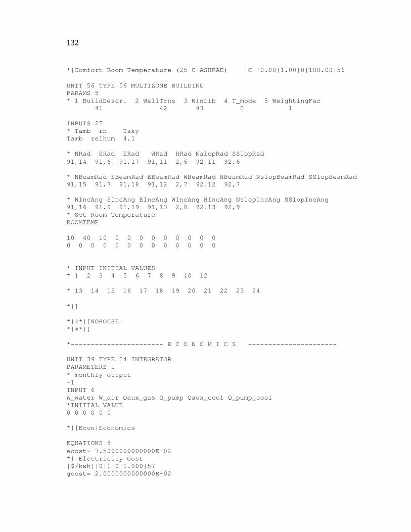
132

*|Comfort Room Temperature (25 C ASHRAE) |C||0.00|1.00|0|100.00|56 UNIT 56 TYPE 56 MULTIZONE BUILDING PARAMS 5 * 1 BuildDescr. 2 WallTrns 3 WinLib 4 T_mode 5 WeightingFac 41 42 43 0 1 INPUTS 25 * Tamb rh Tsky Tamb relhum 4,1 * NRad SRad ERad WRad HRad NslopRad SSlopRad 91,14 91,6 91,17 91,11 2,6 92,11 92,6 * NBeamRad SBeamRad EBeamRad WBeamRad HBeamRad NslopBeamRad SSlopBeamRad 91,15 91,7 91,18 91,12 2,7 92,12 92,7 * NIncAng SIncAng EIncAng WIncAng HIncAng NslopIncAng SSlopIncAng 91,16 91,9 91,19 91,13 2,8 92,13 92,9 * Set Room Temperature ROOMTEMP 10 40 10 0 0 0 0 0 0 0 0 0 0 0 0 0 0 0 0 0 0 0 0 0 0 * INPUT INITIAL VALUES * 1 2 3 4 5 6 7 8 9 10 12 * 13 14 15 16 17 18 19 20 21 22 23 24 *|] *|#*|[NOHOUSE| *|#*|] *----------------------- E C O N O M I C S ---------------------- UNIT 39 TYPE 24 INTEGRATOR PARAMETERS 1 * monthly output -1 INPUT 6 W_water W_air Qaux_gas Q_pump Qaux_cool Q_pump_cool *INITIAL VALUE 0 0 0 0 0 0 *|[Econ|Economics EQUATIONS 8 ecost= 7.5000000000000E-02 *| Electricity Cost |$/kwh||0|1|0|1.000|57 gcost= 2.0000000000000E-02

133

*| Natural Gas Cost |$/kwh||0|1|0|1.000|58 costwater=[39,1]/3600*ecost costair=[39,2]/3600*ecost costgas=[39,3]/3600*gcost costpump=[39,4]/3600*ecost costcool=[39,5]/3600*ecost costpumpcool=[39,6]/3600*ecost Equations 1 deltacost=costair-costwater *|] * --------------------- O U T P U T I N F O R M A T I O N -------------- *|* Output Information *|{PRINTERMODE|Printer Mode *| Show Online Printer ? |ONLINEPRN *|} *|{Outputmode|Output Mode *|General Information (Output 1 : SPAC.OU1) |BuildingPrint *|Energy Information (Output 2 : SPAC.OU2) |PoolenergyPrint *|Weather Information (Output 3 : SPAC.OU3) |Weatherprint1 *|Air-Conditioner Information (Output 4 : SPAC.OU4) |Varcop-Print *|Economic Information (Output 5 : SPAC.OU5) |Econ|Printecon *|System Power Consumption Information (Output 6 : SPAC.OU6)|PowerPrint *|} *|* *|* Press F8 to RUN simulation ! *=================T R N S Y S - O N L Y ================ *---------------- R A D I A T I O N -------------------- UNIT 2 TYPE 16 RADIATION PROCESSOR FOR SWIMMING POOL PARAMS 9 *1 Mode 2 Tracking 3 Rad.mode 4 start_day 7 1 1 STADAY *5 Latitude 6 Solar_const Lat 4871.1 *7 Shift in solar time hour angle (degrees) DevSolar *8 Rad_mode 9 sim-time 2 1 INPUTS 9 * 1 globrad 2Beam_rad 3 Time_last_reading 4 Time_next_reading I Ib TimeLast TimeNext

134

* 5 Gr_reflect 6 Slope/axis 7 AziAngle 8 I_next 9 Ib_next groundref 0,0 0,0 0,0 0,0 * INPUT INITIAL VALUES * 1 2 3 4 5 6 7 8 9 0 0 0 1 0.2 SLOPE ORI 0 0 UNIT 91 TYPE 16 RADIATION PROCESSOR FOR HOUSE PARAMS 9 *1 Mode 2 Tracking 3 Rad.mode 4 start_day 7 1 1 STADAY *5 Latitude 6 Solar_const Lat 4871.1 *7 Shift in solar time hour angle (degrees) DevSolar *8 Rad_smooth 9 sim-time 1 1 INPUTS 15 * 1 Glob_rad 2 Beam_rad 3 Time_last_reading 4 Time_next_reading 5 Gr_reflect I Ib Timelast Timenext groundref * 6 Sl-S 7 Azi-S 8 SL-W 9 Azi-W 10 Sl-N 11 Azi-N 12 Sl-E 13 Azi-E 0,0 0,0 0,0 0,0 0,0 0,0 0,0 0,0 * 14 I_next 15 Ib_next 0,0 0,0 * INPUT INITIAL VALUES * 1 2 3 4 5 6 7 8 9 10 11 12 13 14 15 0 0 0 1 0.2 0 0 0 -90 0 180 0 90 0 0 UNIT 92 TYPE 16 RADIATION PROCESSOR FOR ROOF PARAMS 9 *1 Mode 2 Tracking 3 Rad.mode 4 start_day 7 1 1 STADAY *5 Latitude 6 Solar_const Lat 4871.1 *7 Shift in solar time hour angle (degrees) DevSolar *8 Rad_smooth 9 sim-time 1 1 INPUTS 11

135

* 1 glob_rad 2 beam_rad 3 Time_last_reading 4 Time_next_reading 5 Gr_reflect I Ib TimeLast TimeNext groundref * 6 Sl-S 7 Azi-S 8 SL-N 9 Azi-N 0, 0 0, 0 0, 0 0, 0 * 10 I_next 11 Ib_next 0,0 0,0 * INPUT INITIAL VALUES * 1 2 3 4 5 6 7 8 9 10 11 0 0 0 1 0.2 14 0 14 180 0 0 UNIT 4 TYPE 69 Sky Temperature PARAMS 2 * mode height 0 450 INPUTS 5 * Ta Tdp Ib Id Tamb 3,8 Ib Id 0,0 * INPUT INITIAL VALUES 0 0 0 0 0 *---------------S W I M M I N G P O O L ---------------- EQUATIONS 1 Qpoolin=Qfluidheat+Qcond-Qfluidcool UNIT 143 TYPE 143 PREPOOL - FCOVER PARAMETER 3 * topen tclose settemp topen tclose Tset INPUTS 2 * Tpool fcover 6,1 143,1 *INITIAL VALUES Tpoolstart 0 UNIT 6 TYPE 144 SWIMMING POOL SIMULATION PARAMS 10 * 1 pooltemp_start 2 poolarea 3 poolvol 4 ModeN 5 epsilon_cover Tpoolstart poolarea poolvol 1 poolemis * 6 absorbt 7 Cond_cover 8 Thick_cover 9 Heigth_windspeed poolemis condcov covthick 10 * 10 Shelter_factor sfac INPUTS 15

136

* 1Tamb 2relhum 3windspeed 4RadHori 5Tsky 6Tpoolwall 7HeatTrans Tamb relhum windVel 2,4 4,1 0,0 0,0 * 8mode 9m_dotTab 10Ttab 11open 12close 13maxpeople 14cover% Qpoolin mode 7,1 0,0 0,0 0,0 0,0 Fcover Qpoolin *mPool TpoolIn * INPUT INITIAL VALUES * 1 2 3 4 5 6 7 8 9 10 11 12 13 14 15 16 20 60 0 0 0 0 0 0 0 12 0 0 0 0 0 12 * ---------- TAB WATER ------- UNIT 7 TYPE 14 FORCING FUNCTION PRESIM TYPE 1014 PARAMS 12 0 0 48 0 */48 1000 48 0 58 0 */58 1000 58 0 168 0 * ----------- MAKE UP WATER ---------- *|[RAINMAKER| UNIT 29 TYPE 9 DATA READER - THE RAINMAKER ! PARAMETER 41 * mode #ofvalues timestep 2 12 1 *value mult add -1 1 0 -2 1 0 -3 1 0 -4 1 0 -5 1 0 -6 1 0 -7 1 0 -8 1 0 -9 1 0 -10 1 0 -11 1 0 -12 1 0 *unit# format 11 0 EQUATIONS 13 jan=[29,1] feb=[29,2] mar=[29,3]

137

apr=[29,4] may=[29,5] jun=[29,6] jul=[29,7] aug=[29,8] sep=[29,9] oct=[29,10] nov=[29,11] dec=[29,12] Qevap=[6,3] *|] UNIT 31 TYPE 130 Calculates hourly precipitation INPUTS 12 jan feb mar apr may jun jul aug sep oct nov dec *INITIAL VALUES jan feb mar apr may jun jul aug sep oct nov dec EQUATIONS 3 prewater=[31,1] * waterloss=Qevap/(rho*dh)*3.6 [m3/hr] waterloss = 0.27777*3.6*Qevap/(997.9*(1602.652-6.659528*[6,1])) watergain = prewater/1000*poolarea UNIT 30 TYPE 24 INTEGRATOR INPUT 2 waterloss watergain *INITIAL VALUE 0 0 * -------- O U T P U T ------------ *|[BuildingPrint| ASSIGN C:\spac\spac.ou1 31 UNIT 19 TYPE 25 PRINTER OUTPUT 1 General Information PARAMS 5 *STEP START STOP LOGICAL-UNIT UNITS 1 Start Stop 31 1 INPUTS 6 Tamb 6,1 Tbuild Qdemand Qcond Power Tamb Tpool Tbuild Qhouse Qcond ACPower C C C kJ/hr kJ/hr kJ/hr *|] *|[PoolenergyPrint| ASSIGN C:\spac\spac.ou2 32 UNIT 99 TYPE 25 PRINTER PRESIM TYPE 1125 OUTPUT 2 Energy PARAMS 5 *STEP START STOP LOGICAL-UNIT UNITS 1 start stop 32 1 INPUTS 7 6,3 6,4 6,5 6,7 Qac Qfluidheat Qfluidcool

138

Qevap Qconv Qrad Qsol Qac Qheater Qcooler kJ/hr kJ/hr kJ/hr kJ/hr kJ/hr kJ/hr kJ/hr *|] *|[WEATHERPRINT1| ASSIGN C:\spac\spac.ou3 33 UNIT 100 TYPE 25 PRINTER OUTPUT 3 Weather PARAMS 5 *STEP START STOP LOGICAL-UNIT UNITS 1 START STOP 33 1 INPUTS 5 Ib I Tamb humrat windvel Ib Iglob Tamb humrat windVel kJ/hr-m2 kJ/hr-m2 C % m/s *|] *|[VARCOP-PRINT| ASSIGN C:\spac\spac.ou4 34 UNIT 101 TYPE 25 OUTPUT 4 AC PARAMS 5 *STEP START STOP LOGICAL-UNIT UNITS 1 0 10000 34 1 *T_c_in COP_water W_water QcondW COP_air W_air QcondA INPUTS 8 6,1 44,6 44,4 44,2 Tamb 44,7 44,5 44,3 T_c_in_w COP_water W_water QcondW T_c_in_a COP_air W_air QcondA C - kW kJ/hr C - kW kJ/hr *|] *|[PrintEcon| ASSIGN C:\spac\spac.ou5 35 UNIT 102 TYPE 25 Output 5 Economics PARAMETERS 5 *STEP START STOP LOGICAL-UNIT UNITS -1 Start STOP 35 1 INPUTS 6 costwater costair costgas costpump costcool costpumpcool ac_water ac_air cost_heating pumpheating poolcooling pumpcooling $ $ $ $ $ $ *|] *|[PowerPrint| ASSIGN C:\spac\spac.ou6 37 UNIT 104 TYPE 25 Output 6 Integrated Power Consumption PARAMETERS 5 *STEP START STOP LOGICAL-UNIT UNITS -1 Start STOP 37 1 INPUTS 6 39,1 39,2 39,3 39,5 39,4 39,6 P_AC_water P_AC_air P_heating P_cooling P_pump_heat P_pump_cool

139

kJ kJ kJ kJ kJ kJ *|] *|[waterlossprint| ASSIGN C:\spac\spac.ou7 36 UNIT 103 TYPE 25 PRINTER Output 7 Waterloss PARAMS 5 *STEP START STOP LOGICAL-UNIT UNITS 1 START STOP 36 1 INPUTS 3 waterloss 30,1 30,2 waterloss sumwloss sumwgain m3/hr m3 m3 *|] *\*--------------- O N L I N E P R I N T E R ------------------ *|[ONLINEPRN| UNIT 20 TYPE 65 ONLINE PLOTTER PARAMS 14 * 1#left 2#right 3minylef 4maxylef 5minyrig 6maxyrig 7updateplot 8updatenum 3 0 10 40 0 0 1 1 * 9units 10Npic 11grid 12stop 13symbols 14on/off 3 BILDER GRIDNR 2 2 0 INPUTS 3 * 1Ta 2Tpool 3Tbuild Tamb 6,1 Tbuild *INPUT INITIAL VALUES *1 2 3 Tamb Tpool Thouse LABELS 4 øC øC Temperatures [øC] - *|] END

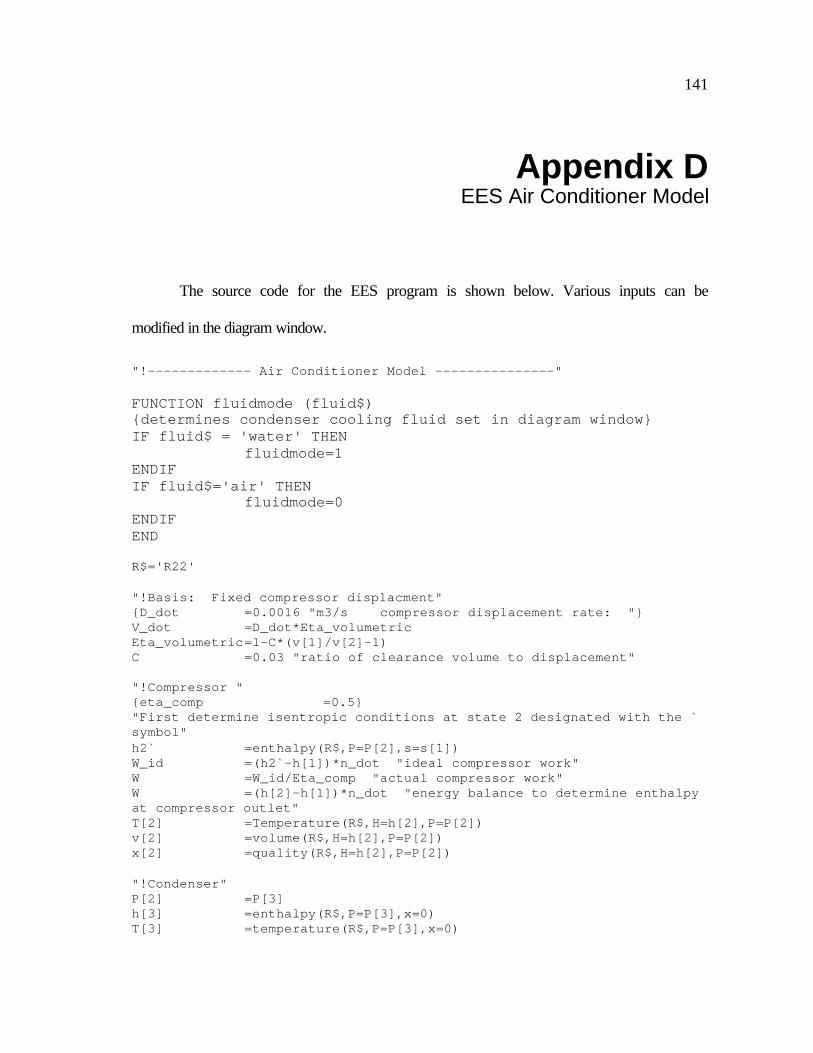
141

Appendix D EES Air Conditioner Model

The source code for the EES program is shown below. Various inputs can be

modified in the diagram window.

"!------------- Air Conditioner Model ---------------" FUNCTION fluidmode (fluid$) {determines condenser cooling fluid set in diagram window} IF fluid$ = 'water' THEN fluidmode=1 ENDIF IF fluid$='air' THEN fluidmode=0 ENDIF END R$='R22' "!Basis: Fixed compressor displacment" {D_dot =0.0016 "m3/s compressor displacement rate: "} V_dot =D_dot*Eta_volumetric Eta_volumetric =1-C*(v[1]/v[2]-1) C =0.03 "ratio of clearance volume to displacement" "!Compressor " {eta_comp =0.5} "First determine isentropic conditions at state 2 designated with the ` symbol" h2` =enthalpy(R$,P=P[2],s=s[1]) W_id =(h2`-h[1])*n_dot "ideal compressor work" W =W_id/Eta_comp "actual compressor work" W =(h[2]-h[1])*n_dot "energy balance to determine enthalpy at compressor outlet" T[2] =Temperature(R$,H=h[2],P=P[2]) v[2] =volume(R$,H=h[2],P=P[2]) x[2] =quality(R$,H=h[2],P=P[2]) "!Condenser" P[2] =P[3] h[3] =enthalpy(R$,P=P[3],x=0) T[3] =temperature(R$,P=P[3],x=0)

142

Q_cond =(h[2]-h[3])*(n_dot) "heat transfer from condenser from an energy balance" Q_cond =epsilon_cond*C_min_cond*(T[3]-T_C_in) "heat transfer rate equation" epsilon_cond =1-exp(-NTU_cond) "effectiveness with Cr=0 (constant temperature condensation)" NTU_cond =UA_cond/C_min_cond "condenser NTU" C_min_cond =C_waterair Q_cond=C_waterair*(T_C_out-T_C_in)"Poolwaterpump-massflowrate=const" c_p =SPECHEAT(Water,T=T_c_in,P=101.3) n_dot_cond=m_dot_cond/MOLARMASS(fluid$) c_air = SPECHEAT(Air,T=T_C_in) "[kJ/kmole-K]" c_water = SPECHEAT(Water,T=T_c_in,P=101.3)"[kJ/kmole-K] C_waterair = (1-fluidmode(fluid$))*n_dot_cond*c_air+fluidmode(fluid$)*n_dot_cond*c_water epsilon_c[1] =epsilon_cond NTU_c[1] =NTU_cond "!Throttle - isenthalpic flashing" x[4] =quality(R$,P=P[4],h=h[4]) h[4] =h[3] T[4] =temperature(R$,P=P[4],h=h[4]) "!Evaporator" P[1] =P[4] h[1] =enthalpy(R$,P=P[1], x=1) v[1] =volume(R$,P=P[1],x=1) s[1] =entropy(R$,P=P[1],x=1) T[1] =Temperature(R$,P=P[1],x=1) V_dot =v[1]*n_dot "this statement determines n_dot, the refrigerant molar flowrate" m_dot =n_dot*MOLARMASS(R$) C_min_evap =Q_evap/(T_E_in-T_E_out) "minimum capacitance rate is the air" Q_evap =epsilon_evap*C_min_evap*(T_E_in-T[4]) "heat transfer rate equation" Q_evap =(h[1]-h[4])*n_dot "evaporator heat transfer rate from an energy balance" NTU_evap =UA_evap/C_min_evap "NTU of evaporator" epsilon_evap =1-exp(-NTU_evap) epsilon_e[1] =epsilon_evap NTU_e[1] =NTU_evap Q_evap =n_dot_evap*c_air_e*(T_e_in-T_e_out) m_dot_evap =n_dot_evap*MOLARMASS(Air) c_air_e =SPECHEAT(Air,T=T_e_in) m_dot_cond=(1-fluidmode(fluid$))*m_dot_air+fluidmode(fluid$)*m_dot_water "TEMPERATURE APPROACH" T[3] =T_c_in+DELTAT_cond DELTAT_cond =DELTAT_water*fluidmode(fluid$)+DELTAT_air*(1-fluidmode(fluid$))

143

T_e_out =DELTAT_evap+T[1] "Volumetric Flows" V_dot_cond=m_dot_cond/DENSITY(fluid$,T=T_c_in,P=101.3)/MOLARMASS(fluid$) V_dot_cond_cfm=V_dot_cond*convert(m^3/s, cfm) V_dot_evap =m_dot_evap/DENSITY(air,T=T_e_in,P=101.3)/MOLARMASS(air) V_dot_evap_cfm=V_dot_evap*convert(m^3/s, cfm) "!end of ac-model" "!System" COP =Q_evap/(W+W_dot_fan+W_dot_pump+W_dot_fan_evap) W_total =W+W_dot_fan+W_dot_pump+W_dot_fan_evap EER =q_evap*convert(kW,Btu/hr)/ ((W+W_dot_fan+W_dot_pump)*convert(kW,W)) "! FAN-tastic" {N_ref =2800 "[rpm]"} {d =28*convert(inch,m) "[m]"} {W_dot_ref =0.345 "[kW]"} {V_dot_ref =2800*convert(cfm, m^3/s) "[m^3/s]"} V_dot_ref =V_dot_ref_cfm*convert(cfm, m^3/s) W_dot_ref =C_w*(N_ref*convert(rpm, rps))^3*d^5*rho*convert(W, kW) V_dot_ref =C_v*N_ref*convert(rpm, rps)*d^3 rho =DENSITY(air,T=20,P=101.3)*MOLARMASS(air) "[kg/m^3]" "Fanlaws" W_dot_fan =C_w*(N*convert(rpm, rps))^3*d^5*rho*convert(W, kW)*(1-fluidmode(fluid$)) V_dot_fan =C_v*N*convert(rpm, rps)*d^3 V_dot_fan =V_dot_cond W_dot_fan_evap =C_w*(N2*convert(rpm, rps))^3*d^5*rho*convert(W, kW) V_dot_fan_evap =C_v*N2*convert(rpm, rps)*d^3 V_dot_fan_evap =V_dot_evap "!PUMP-astic" rho_pump =DENSITY(water,T=T_C_in,P=101.3)*MOLARMASS(water) "[kg/m^3]" W_dot_pump=DELTAp_v*V_dot_pump*convert(W,kW)/eta_pump DELTAp_v =ceta*rho_pump/2*v_pump^2 "[kg/m-s^2]" ceta =1 v_pump =V_dot_cond/A_pipe "[m/s] velocity of water" A_pipe =d_pipe^2*pi/4 "[m^2]" {d_pipe =0.015 "[m]"}

144

V_dot_pump =V_dot_cond*fluidmode(fluid$)

use of air conditioning heat rejection for swimming pool

Documents