User-Constrained Algorithms for Aggregate Residential Demand Response Programs with Limited Feedback.

by

Adam Charles Gray B.Eng., University of Victoria, 2011

A Thesis Submitted in Partial Fulfillment of the

Requirements for the Degree of

Master of Applied Science

in the Department of Mechanical Engineering

© Adam Charles Gray, 2015 University of Victoria

All rights reserved. This thesis may not be reproduced in whole or in part, by photocopying or other means, without the permission of the author.

ii

User-Constrained Algorithms for Aggregate Residential

Demand Response Programs with Limited Feedback.

by

Adam Charles Gray

B.Eng., University of Victoria, 2011

Supervisory Committee

Dr. Curran Crawford, (Department of Mechanical Engineering)

Supervisor

Dr. Ned Djilali, (Department of Mechanical Engineering)

Departmental Member

iii

Abstract

Supervisory Committee

Dr. Curran Crawford, (Department of Mechanical Engineering)

Supervisor

Dr. Ned Djilali, (Department of Mechanical Engineering)

Departmental Member

This thesis presents novel algorithms and a revised modeling framework to evaluate residential

aggregate electrical demand response performance under scenarios with limited device-state

feedback. These algorithms permit the provision of balancing reserves, or the smoothing of

variable renewable energy generation, via an externally supplied target trajectory. The responsive

load populations utilized were home heat pumps and deferred electric vehicle charging. As fewer

devices in a responsive population report their state information, the error of the demand response

program increases moderately but remains below 8%. The associated error of the demand response

program is minimized with responsive load populations of approximately 4500 devices; the

available capacity of the demand response system scales proportionally with population size. The

results indicate that demand response programs with limited device-state feedback may provide a

viable option to reduce overall system costs and address privacy concerns of individuals wishing

to participate in a demand response program.

iv

Table of Contents

Supervisory Committee ....................................................................................................... ii

Abstract ............................................................................................................................... iii

Table of Contents ................................................................................................................ iv

List of Tables ..................................................................................................................... vii

List of Figures ................................................................................................................... viii

List of Abbreviations and Symbols ..................................................................................... x

Acknowledgements .......................................................................................................... xiv

1 Introduction .................................................................................................................. 1

1.1 Motivation. .......................................................................................................... 1

1.2 Main Contributions ............................................................................................. 2

1.3 Thesis Structure .................................................................................................. 3

2 Aging Infrastructure and Increasing Demand .............................................................. 4

2.1 Conventional Electrical Generation Resources .................................................. 4

2.1.1 Renewable Energy: Variable Generation Resources .................................. 5

2.2 Conventional Power System Operations ............................................................ 6

2.3 Addressing Increased Variability of Renewable Generation .............................. 7

2.3.1 Energy Storage Resources .......................................................................... 8

2.3.2 Demand Response Programs ...................................................................... 9

2.3.3 Demand Response Applications ................................................................ 11

2.3.4 Privacy Concerns in Demand Response Systems ..................................... 11

2.4 Identifying suitable loads for Direct Demand Response .................................. 12

2.4.1 Thermostatically controlled loads ............................................................. 13

v

2.4.2 Energy storage as a deferrable load .......................................................... 14

2.4.3 Hysteresis control of deferrable loads....................................................... 15

2.5 Managing Aggregate Load Demand ................................................................. 17

2.5.1 Controlling Load Community Dynamics.................................................. 18

2.5.2 Dispatch of multiple loads ........................................................................ 21

3 Computational Modeling Framework ........................................................................ 24

3.1 Demand-side: Load Models .............................................................................. 24

3.1.1 Heat Pump Equivalent Thermodynamic Parameter Model ...................... 24

3.1.1.1 Heat Pump Unit Sizing .................................................................................................... 26

3.1.1.2 Heat Pump ETP Model Example ................................................................................. 27

3.1.2 Plug-in Electric Vehicle charging Model ................................................. 28

3.1.2.1 PEV Charging Model Example ...................................................................................... 29

3.2 Supply-side: Power System Model ................................................................... 31

3.2.1 Wind Energy Generation .......................................................................... 31

3.3 Selecting the Simulation Time-step .................................................................. 34

4 Demand Response Algorithms ................................................................................... 35

4.1 Accounting for Limited Knowledge of Load States ......................................... 35

4.2 Control Performance Metrics ............................................................................ 36

4.2.1 RMS Error % ............................................................................................ 36

4.2.2 Load Flexibility/Under-utilization factor .................................................. 37

4.3 Model Input Data .............................................................................................. 38

4.3.1 Environmental Data - Air Temperature & Wind Speed ........................... 38

4.3.2 Thermodynamic Data - Heat Pump Sizing and ETP values ..................... 39

4.3.3 PEV Data - Vehicle sizing & charging schedules .................................... 40

4.3.4 Target Trajectory ...................................................................................... 42

4.3.4.1 Regulating Reserve Dispatch Signal .......................................................................... 44

4.3.4.2 Reducing Variability of Wind Generation Target Signal .................................... 45

5 Model Results ............................................................................................................. 48

5.1 Provision of Wind-Generation Smoothing Services ......................................... 48

vi

5.1.1 Limited-knowledge Population Dynamics ............................................... 52

5.1.2 Capacity Determination for Wind-Generation Smoothing ....................... 55

5.2 Provision of Regulating Reserve Ancillary Services ........................................ 57

5.2.1 Limited-Knowledge Population Dynamics............................................... 62

5.2.2 Capacity Determination for Ancillary Service Provision ......................... 66

6 Conclusions ................................................................................................................ 72

6.1 Main Contributions ........................................................................................... 72

6.2 Recommendations for Future Work.................................................................. 74

7 References .................................................................................................................. 76

vii

List of Tables

Table 2.1 - Cost and Emissions Data for Large-scale Generating Technologies [7], [12],[13]. .... 4

Table 2.2 - Cost of Various Storage Technologies [25]. ................................................................ 8

Table 3.1 - Parameters implemented in the heat pump ETP model.............................................. 27

Table 3.2 - Parameters implemented in the EV charging model. ................................................. 30

Table 3.3 - Parameters implemented in the wind energy system model [7]. ................................ 33

Table 4.1 - ETP Model Input Parameters. .................................................................................... 39

Table 4.2 - PEV Charging model input parameter distribution data ............................................ 41

Table 5.1 - Performance of Load Resources Performing Wind Smoothing Services. ................. 52

Table 5.2 - Performance of Load Resources Performing Balancing Services. ............................. 62

viii

List of Figures

Figure 2.1 – BPA Balancing Authority Load & Total Wind, Hydro, and Thermal Generation 16

Oct 2014 – 23 Oct 2014 [19]. ................................................................................................. 6

Figure 2.2 - Closed-loop control strategy implemented. .............................................................. 20

Figure 3.1 - ETP Schematic [7]. ................................................................................................... 25

Figure 3.2 - Example of the ETP model response under the displayed outdoor temperature profile.

............................................................................................................................................... 28

Figure 3.3- Example of the EV load model. ................................................................................. 30

Figure 3.4 - Sample wind speed data (top panel) and resultant model wind generation data (bottom

panel)..................................................................................................................................... 33

Figure 4.1 - Representative outdoor air temperature and wind speed data from NWTC M2 tower.

............................................................................................................................................... 38

Figure 4.2 - Scatterplot showing selected ETP parameters for a population of 1500 heat pumps.

............................................................................................................................................... 40

Figure 4.3 - Scatterplot showing PEV charging start and end times. ........................................... 41

Figure 4.4 - Recharge access by time of day (BC only, n=528, 3-day driving diary) [53]. ......... 42

Figure 4.5 - BPA Balancing Reserves Available & Dispatched July 31 - Aug 7, 2014 [19] ....... 44

Figure 4.6 - Frequency distribution of BPA balancing reserves dispatched data from 2014 (left

panel) and 24-hour simulation period (right panel). ............................................................. 45

Figure 4.7 - Sample target trajectory and net grid power injections based on wind generation profile

from section 3.2.1. ................................................................................................................ 46

Figure 4.8 - Frequency distribution data for NREL wind speed data from 2014 (left panel) and 24-

hour simulation period (right panel). .................................................................................... 47

Figure 5.1 - Wind Generation Smoothing Target Trajectory ....................................................... 48

Figure 5.2 - Wind Generation over 24-hour Simulation Period. .................................................. 49

Figure 5.3 - Demand Response System trajectories. .................................................................... 50

Figure 5.4 - Individual VGM flexibility and under-utilization factors. ........................................ 51

Figure 5.5 - Density plots of VGMs. ............................................................................................ 51

Figure 5.6 - System response and Target trajectory under limited-knowledge simulations. ........ 53

ix

Figure 5.7 - NRMSE associated with varying levels of device-state knowledge for wind-firming

target trajectory. .................................................................................................................... 54

Figure 5.8 - Individual VGM response for 100%, 80%, and 50% knowledge scenarios. ............ 54

Figure 5.9 - NRMSE associated with individual VGM populations for various knowledge levels.

............................................................................................................................................... 55

Figure 5.10 - Energy Dispatched by VGMs (top panel) and Mean Available VGM Capacity

(bottom panel) for Various Load Community Population Sizes. ......................................... 56

Figure 5.11 - Scaled target trajectory & VGM feasible region boundaries. ................................. 57

Figure 5.12 - Uncontrolled and Controlled Population Response. ............................................... 58

Figure 5.13 - Individual VGM Feasible Regions, Target Trajectory, and Actual Response. ....... 59

Figure 5.14 - VGM Flexibility and under-utilization factors. ...................................................... 60

Figure 5.15 - Load Community Power Distributions. .................................................................. 61

Figure 5.16 – Aggregate system response under limited-knowledge simulations........................ 63

Figure 5.17- NRMSE for Different Levels of Device-State Reporting. ....................................... 64

Figure 5.18 - Individual VGM response for 100%, 80%, and 50% knowledge scenarios. .......... 65

Figure 5.19 - NRMSE associated with individual VGM populations for various knowledge levels.

............................................................................................................................................... 65

Figure 5.20 - Energy Dispatched vs Population Size for 100% Knowledge Scenarios. .............. 67

Figure 5.21 - NRMSE of Responsive Load Populations of Various Sizes under Limited Device-

state Information Scenarios................................................................................................... 68

Figure 5.22 - Mean Available Capacity of VGMs vs Population Size. ........................................ 69

Figure 5.23 – Heat Pump VGM control signal magnitude and variability for various population

sizes and device-state knowledge scenarios. ........................................................................ 70

x

List of Abbreviations and Symbols

Abbreviations

AMSL Above Mean Sea Level

BPA Bonneville Power Authority

CAES Compressed Air Energy Storage

CAISO California Independent System Operator

CCGT Closed Cycle Gas Turbine

CPEVS Canadian Plug-in Electric Vehicle Survey

DR Demand Response

EC Electrochemical Capacitors

ETP Equivalent Thermodynamic Parameter

EV Electric Vehicle

GHG Green House Gas

HVAC Heating, Ventilation, and Air-Conditioning

LA Load Aggregator

LC Load Community

NREL National Renewable Energy Laboratory

NRMSE Normalized Root Mean Squared Error

O & M Operations & Maintenance

OCGT Open Cycle Gas Turbine

PCH Programmable Communicating Hysteresis Controller

PEV Plug-in Electric Vehicle

PHS Pumped Hydro Storage

SMES Superconducting Magnet Energy Storage

TCL Thermostatically Controlled Load

TOU Time of Use

VGM Virtual Generator Model

xi

Symbols

Ca Indoor air thermal mass

Cm Indoor building thermal mass

Cp Wind turbine coefficient of performance

Cp,m Turbine coefficient of performance at maximum wind speed

Cp,r Turbine coefficient of performance at rated wind speed

D Wind turbine blade diameter

e Additional un-modeled system gains or losses (White noise term)

E State of Charge of EV Battery

EC PEV Battery Capacity

��(�) Total energy dispatched from responsive load population p

ES Minimum required charging trajectory

i Population index

k Discrete time sampling index

m Deadband location index

n Operational State of Load

Ni Number of loads in population

Np Number of responsive load communities

p Responsive load type index

P Current Device Power Consumption

P0 Uncontrolled responsive load trajectory ���� Total installed capacity in responsive load population

Pcap Total power rating of aggregate responsive load population

Ph Required electric power of heat pump at design temperature

Pfan Required electric power of heat pump fan

Pm Mechanical power imparted to wind turbine blades

Pmin Minimum responsive load population power output

Pmax Maximum responsive load population power output

Pr,i Rated power of individual load

Prt Turbine rated power

PT Aggregate target trajectory for multiple responsive load communities

xii

Pwind Total power generated from wind turbine

P* Target trajectory for individual responsive load population

ΔP* Target deviation from uncontrolled responsive load trajectory

S Turbine gearbox number of stages

T Sampling time interval (1 min)

TS Simulation Time Period

u DR set point modulation control signal

uci Turbine cut-in speed

uco Turbine cut-out speed

um Turbine maximum wind speed

ur Turbine rated wind speed

us* Target modulation control signal Wind speed q� Total heat input to system �� Design heating rate of the heat pump ���� Heating power of heat pump fan operation �� Heating rate of heat pump �� ���� Rate of Heat transfer from house to environment �� �� Rate of heat transfer from heat pump to indoor air

Rao Building envelope heat transfer resistance

Rma Heat transfer resistance between building mass and air

Z Set of power state vectors

zi Individual load device power state vector � Wind turbine blade pitch angle

δ Hysteresis control deadband width �� Device State-transition lower boundary �� Device State-transition upper boundary � Device End-use state comparison �� Outdoor air temperature �� Heat pump system design temperature �� Thermostat temperature set point

xiii

θ� House thermal mass temperature θ�� Thermal trajectory of home indoor air θ�� Thermal trajectory of home thermal mass Ω ETP State-transformation matrix Γ ETP Input-transformation matrix # Wind turbine tip-speed ratio $ Air density % Energy Conversion Efficiency

ηd Heat pump efficiency at design temperature &' Turbine electrical conversion efficiency &( Turbine gearbox efficiency Φ Capacity factor of responsive load population Φ*+,+-'� Capacity factor of reporting loads in responsive population ./ Inactive power density distribution function .0 Active power density distribution function ./,2 Inactive power density distribution function of reporting loads .0,2 Active power density distribution function of reporting loads ℱ(�) Flexibility of responsive load population p 4�5� Down-regulation under-utilization factor 46� Up-regulation under-utilization factor 7 Heat pump oversize factor

xiv

Acknowledgements

I would like to thank Curran Crawford for inspiring me to pursue research in the field of energy

systems modeling, as well as providing me with the resources and tools necessary to effectively

complete this project. I would also like to thank Ned Djilali and David Chassin, along with the

many other amazing researchers at the Institute for Integrated Energy Systems at the University of

Victoria (IESVic), whom provided valuable insight and a grounded sounding board for my

research ideas, as well as their technical implementation. The employees at the Bonneville Power

Authority (BPA) and National Renewable Energy Laboratory (NREL) were instrumental in

obtaining relevant environmental input data, as were my colleagues at Simon Fraser University

and the University of Victoria involved in the CPEVS project. Further, I would like to thank

CIMTAN and NSERC for providing funding throughout my studies, without which it would not

have been possible.

Finally, I would like to thank my friends and family, for always encouraging my studies while

keeping me grounded in reality.

1

1 Introduction

1.1 Motivation.

As global warming and GHG emissions are becoming a critical issue around the world, there is

increasing investment in renewable electrical generation technologies and a shift to electrification

of transportation [1]. While there has been a strong push in the development of renewable

generation facilities, particularly solar photovoltaic, wind turbine generation, and micro-hydro or

run-of-river generation technologies, the infrastructure to support the integration of such inherently

variable generation resources is struggling to keep up [2]. Electric utilities must ensure that reliable

electricity is constantly available to users when they desire it, and as the penetration of variable

renewable generation increases, the stress put on the conventional generation and distribution

systems can be pushed to its limits [3]. Further complicating the problem is that electrical demand

continues to increase, with BC Hydro projecting a 1.7% annual increase in demand over the next

20 years [4].

One area that exhibits considerable flexibility in addressing the variability of renewable

generation, as well as conventional power systems operating requirements, is demand response

(DR). Rather than treating electrical loads as strictly must-serve entities, the integration of demand

response programs via the smart grid enables the deferral of certain electrical loads to more

opportune times. Generally demand response programs are deployed utilizing large commercial

and industrial loads as they are of sufficient size to easily integrate into a conventional electrical

power system [5], [6]. However, recent work has been completed to show that an aggregate

population of residential scale loads, specifically home heating using air source heat pumps, and

electric vehicle charging loads, are capable of providing significant ancillary services capacity to

electrical system operators [7], [8]. One of the key considerations in this work is that consumer

comfort constraints and end-use functionality of the individual appliances must remain a primary

objective of the controllers. This ensures that consumers will be willing to participate in the

demand response program, and minimizes the inconvenience caused to individual consumers

while still maintaining a robust demand response system to the power systems operator.

2

One of the major hurdles to widespread adoption of residential demand response programs is the

cost of communications infrastructure, coupled with individual privacy concerns related to the

device-state information being used in the demand response control algorithms [9]. This thesis will

examine the ability to implement a demand response program for aggregate populations of

residential deferrable loads using limited device-state information from a portion of the

participating population. In this manner, it is hoped that widespread adoption and participation in

demand response programs will be possible with reduced communications infrastructure costs, and

the ability for a subset of a population to participate in the demand response program without

reporting any device-state information, thus alleviating privacy concerns.

1.2 Main Contributions

Many control strategies have been implemented in previous works, but some of the most promising

appear to be centralized control using aggregators, similar to that described in Parkinson [7]. This

thesis will focus on centralized control DR algorithms based on Parkinson’s previous work,

employing a similar DR control system to provide power systems operators with virtual generation

capable of providing ancillary services or renewable energy smoothing. The need for full

information of all participating loads is investigated, with an aim to reduce the instrumentation and

knowledge requirements for successful DR control. In particular, this thesis offers the following

main contributions:

1. The development of a refined computational model capable of simulating various DR

algorithms for populations of any number of residential heat pumps and plug-in electric

vehicles using either a de-centralized or centralized controller, as well as optimal dispatch

among multiple populations for unlimited time periods.

2. A preliminary evaluation of the capacity that load communities of heat pumps and plug-

in-vehicles are capable of providing to the grid when employed as regulating reserve virtual

generation, and when employed to smooth wind generation injections into the grid.

3. A novel control strategy to accurately manage multiple populations of electrical loads to

provide ancillary services to the power system, incorporating limited knowledge of a

portion of the population’s device-states within the system. This system maintains the

ability to simultaneously balance grid-side objectives with the customer comfort-

3

constraints commonly expected by consumers on the demand-side, while further

addressing the privacy concerns of the population.

4. An investigation into the effects of limited device-state information from a sub-group of a

load community on its ability to provide effective demand response, and the impacts of the

number of responsive loads recruited into such a load community on the available capacity

of the demand response program.

1.3 Thesis Structure

This thesis proceeds as follows: Chapter 2 provides an overview of conventional power systems

operation. This chapter identifies a number of challenges associated with the increased penetration

of distributed renewable generation resources, and some of the techniques used to address them.

In particular, emphasis is placed on demand response programs, including the introduction of a

novel demand response approach proposed by Parkinson [7], as it is the theoretical basis for the

work presented in this thesis. Chapter 3 describes the models used to simulate participating loads

employed in the subsequent demand response programs. The participating loads modeled are

residential heat pumps, and plug-in electric vehicle charging. Chapter 4 introduces the concept of

providing user-constrained demand response capabilities with limited knowledge. A

computational framework is developed that permits the provision of ancillary services via demand

response from an aggregate load community, even under scenarios where full knowledge of

individual load-states is unavailable. The provision of ancillary services, as well as smoothing of

wind energy injections into the grid are investigated. Chapter 5 presents the results of various

simulations utilizing these demand response control algorithms, as well as an analysis of the

available capacity these load communities can contribute to power systems operation. Chapter 6

concludes the thesis, providing a summary of key findings and recommendations for future work.

4

2 Aging Infrastructure and Increasing Demand

The current electrical generation and distribution systems are optimized for large,

dispatchable generation facilities that are able to respond to fluctuations in electrical power

demand in real-time through frequent throttling of available fast-acting generation

resources. This arrangement has worked successfully for many years, however with the

increase in non-dispatchable generation it is being pushed to its limits and not operated in

the most efficient manner possible [7], [10]. Not only does the operation of generation

resources in this manner reduce equipment lifetime, it also results in inefficient operations

and increased GHG emissions.

2.1 Conventional Electrical Generation Resources

Canada has a fairly clean energy portfolio, with over 60% of electrical generation being

produced from clean sources [11]. However, in order to meet increasing demand additional

generation projects will be required in the coming years [4]. The costs associated with a

variety of modern generation technologies are summarized in Table 2.1 [7], [12], [13].

Table 2.1 - Cost and Emissions Data for Large-scale Generating Technologies [7], [12], [13].

Technology Overnight Capital Cost

[$/kW]

Fixed O&M Costs [$/kW-yr]

Variable O&M Costs

[$/MWh]

Emissions [tCO2/MWh]

Hydroelectric $2936 $14.13 0.00 0.009

Nuclear $5530 $93.28 $2.14 0.012

Coal $3591 $45.65 $5.85 0.980

CCGT $825 $7.19 $12.91 0.450

OCGT $970 $14.27 $3.44 0.650

Wind $2213 $39.55 $0.00 0.015

Solar PV $4028 $26.22 $0.00 0.061

As shown in Table 2.1, wind generation has one of the largest initial construction costs of

generation technologies, however fuel costs are non-existent and O&M costs are among

the lowest. Although both nuclear and hydroelectric generation produce slightly less

5

lifetime emissions, their initial construction costs are extremely high. Furthermore, there is

political, environmental, and societal opposition to both nuclear and large-scale

hydroelectric generation projects [14], [15]; and, few feasible locations to implement large-

scale hydroelectric projects remain un-utilized throughout Canada [16]. One particular

large scale hydroelectric project currently under consideration is the Site C Dam on the

Peace River in Northeastern British Columbia. The Site C Dam is one of the last feasible

locations for such a project in the Province, and preliminary cost estimates have reached as

high as $7000/kW of installed capacity [17]. In addition to higher than average construction

costs, there is significant opposition to the Site C Dam project on account of environmental

and societal grounds.

These factors, coupled with increased public and political pressure to reduce GHG

emissions of new generation projects has resulted in significant increases in development

of new renewable energy projects [4], [18]. In particular, BC Hydro has been mandated to

increase overall grid system efficiency, with a focus on renewable energy generation

projects as a part of the BC Clean Energy Act [4]. However the majority of renewable

energy generation technologies being considered are inherently variable in nature,

requiring additional investment in infrastructure to ensure reliable integration with the

electrical grid.

2.1.1 Renewable Energy: Variable Generation Resources

One of the primary challenges that arises from increased renewable generation into the

electrical grid is that it both variable and non-dispatchable. Many renewable generation

technologies (solar, wind, tidal, wave, etc.) only produce electricity during periods when

their associated resource flux is available – generation output depends on the solar

insolation, wind speed, tidal flow, or wave action, respectively. They will generate

electricity when the natural resource is abundant, but will reduce or cease to generate any

electricity during periods of reduced resource availability. This non-dispatchable

generation requires power systems operators to balance load with additional generation by

throttling other dispatchable generation resources to compensate. As a result, increased

variable renewable energy generation requires significant dispatchable generation capacity

to be in place at all times, regardless of whether it is running or simply in standby mode.

6

One example of the variability of renewable generation, and the resultant temporal

mismatch between renewable generation and load profile is shown in Figure 2.1[19].

Figure 2.1 – BPA Balancing Authority Load & Total Wind, Hydro, and Thermal Generation 16 Oct

2014 – 23 Oct 2014 [19].

As shown in Figure 2.1, there is no guarantee that the renewable generation will occur at

the same time as periods of increased demand. As a result, it is necessary to either store

excess energy when it is produced for use at a later time, or to curtail generation when it

exceeds demand and rely on dispatchable generation to top-up renewable generation when

it does not meet demand. Not only is this operating approach expensive, but it is also

inefficient and results in additional GHG emissions from dispatchable generation operating

outside of optimal efficiency parameters to match electrical demand and renewable energy

generation [7].

2.2 Conventional Power System Operations

The process used by modern utility operators to achieve the required balance between

generation and demand is a highly regulated and complex process, spanning operations at

the millisecond level up to generation planning studies looking multiple decades into the

future. Long-term planning operations are necessary to ensure that adequate generation

resources are built to meet anticipated future demand, while daily and hourly bidding

operations are used to optimally dispatch available generation resources while reducing

operating costs and maintaining system stability.

Oct 16 Oct 17 Oct 18 Oct 19 Oct 20 Oct 21 Oct 220

1000

2000

3000

4000

5000

6000

7000

8000

Date/Time

MW

BPA Balancing Authority Load & Total Wind, Hydro, and Thermal Generation 16 Oct 2014 - 23 Oct 2014

Load Wind Thermal Hydro

7

Electrical generation is generally categorized as one of the following three types to permit

modern electrical operations and planning [20]:

1. Base-load generation – the slowest responding and largest capacity generation,

suitable to provide large quantities of stable power over long time periods.

Generally these are large thermal generation facilities, large scale hydroelectric, or

nuclear power plants. These facilities run uninterrupted throughout the year with

the exception of maintenance shutdowns.

2. Intermediate generation - runs essentially continuously, but only during certain

periods of the year. It provides additional power to the electrical grid to account for

seasonal variations in electrical consumption. And,

3. Peak generation - the generation capacity to respond to daily variations in

electrical demand. It is fast acting and able to rapidly ramp up and down, but is

typically the most expensive generation to operate.

With the integration of variable renewable energy into the electrical grid, the dispatch of

peak generation resources becomes more variable to ensure system generation can meet

demand. The scheduling and economic dispatch of generation assets within an electrical

grid is in itself a complex subject, with many factors affecting the price paid for generation

depending on the purpose and capabilities of the generation resource. Typically, however,

fast-acting generation resources that can respond to rapid variations in electrical demand

are the most expensive generation to purchase at the wholesale level. These resources are

commonly referred to as regulating or balancing reserves, and are required due to variations

in electrical demand ranging from 1 to 30 minutes – very similar timescales to the

commonly observed short-term variability of wind, solar, and wave energy generation [22].

As a result, increased penetration of renewable generation into an electrical grid can result

in the need to dispatch greater amounts of regulating or balancing reserves, increasing

overall operating costs and GHG emissions [7].

2.3 Addressing Increased Variability of Renewable Generation

There are a number of potential solutions to address the variability that comes with

increased renewable generation in the electrical grid, each with its own unique benefits and

challenges. Operating dispatchable generation resources to firm-up renewable generation

8

is effective, but results in additional GHG emissions and increases the costs of renewable

generation projects when firming power capacity is taken into consideration [22]. The

primary solutions that are robust enough for wide-scale grid integration of variable

renewable generation are dedicated energy storage resources, and demand response

programs [23], [24]. The following sections will briefly discuss both of these potential

solutions as well as some of their benefits and limitations.

2.3.1 Energy Storage Resources

Energy storage resources have seen a surge of development in the last century, resulting in

feasible solutions for long-term storage and fast-acting short term storage technologies;

however they remain expensive to purchase and operate at utility-scale capacities [25],

[26]. Table 2.2 provides a summary of the costs of common storage technologies, as well

as their respective round-trip energy efficiencies.

Table 2.2 - Cost of Various Storage Technologies [25].

Technologies Energy Cost

[$/kWh]

Power Cost

[$/kW]

Balance of Plant Cost

[$/kW or $/kWh]

O & M Cost

[$/kW]

Efficiency

[%]

Lifetime

[years]

CAES 10 450 160 $/kW 6 70 30

PHS 12 2000 2 $/kWh 3 80 40

Pb-acid 300 450 100 $/kW 10 75 6

Li-ion 1500 1500 100 $/kW 10 93 15

Flywheels 1,000 350 100 $/kW 18 90 15

SMES 10,000 300 1,500 $/kWh 10 95 20

EC 30,000 300 100 $/kW 13 95 30

One common theme among grid-scale energy storage technologies is a relatively high

combined cost of storage, and a less than ideal efficiency of energy conversion resulting in

considerable round-trip energy losses. In addition, these storage facilities must be designed

for the largest variations in renewable energy fluctuations, resulting in significant idle

storage capacity during normal operation [25]. Despite these limitations, distributed

storage has emerged as a viable solution to addressing issues related to variability of

renewable generation and grid-side ancillary services [27], [28].

9

2.3.2 Demand Response Programs

Demand response programs are not new – in fact, they have been implemented historically

by power systems operators as a last resort through the practice of systematic load shedding

to prevent blackouts [29]. Modern demand response programs have become more elegant,

taking into consideration the impacts of the program on end-users, coupled with operating

principles to achieve the greatest benefit to the electrical system operator without

interfering with the end-use function of the participating. These programs can be broken

down into two categories depending on how they interact with participating loads: indirect

demand response (price signals), and direct demand response. Each of these types of

demand response system can be implemented using a distributed or centralized controller,

depending on the system performance desired and operating constraints of the program.

Indirect DR provides control of participating loads without specific knowledge of

individual device-states or operating characteristics - one common example being time of

use (TOU) pricing schemes, where the cost of electricity is variable throughout the day in

response to demand and availability of generation resources. Despite not knowing the

specific device-states of participating loads, it is possible for a utility operator to estimate

the resultant system response to a specific price signal. This approach can be effective at

influencing the demand curve, particularly for peak-shaving or valley-filling objectives

[30], [31], however it is often difficult to accurately predict the system response to a change

in price signal as it depends on a number of independent and difficult to predict variables

[32]. Recent work has been undertaken on this particular issue by Pacific Northwest

National Labs, wherein the price signal is incorporated into an autonomous control system

using proprietary thermostats and communications infrastructure [20]. This approach

interfaces very well with conventional time-of-use utility pricing schemes, while

improving the accuracy of the response obtained from an indirect DR program.

Direct demand response provides a much more predictable system response to a control

signal by directly influencing device behaviors based on known device-state information.

As a result, direct demand response programs require that participating loads are equipped

with sufficient communications devices to transmit and receive device-state data and

control signals from the demand response system operator. The advantage to direct DR

systems is that the response of the participating population is much more accurately known,

10

and can be controlled to a high degree of precision [33]. The cost of this high degree of

predictability and control is that the end-use functionality of the participating devices is

more likely to be disrupted if not carefully controlled – customer comfort constraints must

be clearly indicated and compensated for in the control algorithm development to ensure

the DR program does not produce unacceptable device behavior [34].

Both direct and indirect demand response programs exhibit considerable advantages when

compared to energy storage systems for grid-scale applications:

1. The round-trip efficiency of demand response programs can approach 100%, as the

deferred energy is stored as the end-use product (home heat, or EV battery charge,

for example). This contrasts energy storage systems that have inherent

inefficiencies in the energy storage process itself [7], [25].

2. The costs of demand response programs are much smaller than similarly sized

energy storage systems, as the loads themselves are utilized as storage mediums.

The only additional costs are associated with the communications infrastructure,

and is largely already available as smart meters and smart grids are rolled out across

North America [34].

3. Demand response programs, particularly aggregate residential load demand

response programs are easily scalable, and can be expanded as required by

recruiting additional loads to participate in the program [8].

These factors make demand response programs a leading candidate to aid power systems

operators in dealing with variable renewable generation, as well as to provide conventional

ancillary services to electrical grid operations. It should be noted, however, that while

demand response programs are well-suited to provide balancing reserves, they do not

provide net energy to the electrical grid, nor are they suitable to directly provide substantial

grid stability services at this point in development [20].

In addition to the selection of the type of demand response program, be it direct or indirect,

selection of an appropriate control structure is also important in establishing DR resources.

Aggregate controllers reduce computational complexity and individual hardware

requirements for participating loads, as the computationally intensive portion of the control

system is located at a central area. Distributed control, on the other hand, requires

individual device controllers to determine the optimal dispatch of each device

11

independently of other participating loads. This has the advantage of reducing the overall

computational complexity of the control system, and distributing tasks among multiple

agents in the system, however it comes at the expense of processing time and individual

device controller costs.

It may be possible to strike a balance between indirect and direct control through the use

of an aggregate control structure in a direct control setting under limited information

scenarios. If a sample of a participating population is sampled to determine the anticipated

system response, it may be possible to maintain full control authority of the non-reporting

loads in the population. This would serve to reduce the instrumentation requirements of a

direct demand response approach, while maintaining the benefits of predictable system

response.

2.3.3 Demand Response Applications

Demand Response programs have a wide variety of applications in the operation of the

electrical power system. The rapid variation of electrical loads is useful from a system

balancing perspective, reducing the amount of conventional balancing reserves that must

be dispatched to maintain overall energy balance of the grid. In addition to basic energy

balance operations, it is also possible to use demand response programs to improve system

operations and planning models. A group of responsive loads from a similar geographical

area could be used to maintain maximum utilization of transmission lines, as well as to

protect distribution equipment from overload conditions. With the correct control

algorithms, it is possible to utilize demand response programs for ancillary services, grid

stability and security operations, and targeted localized transmission system operation [36].

Even in places like British Columbia, where 90% of generation is from highly dispatchable

hydroelectric facilities, demand response programs can be utilized to optimize the

transmission and distribution grid assets, as well as provide greater flexibility in optimizing

the water levels in reservoirs at hydroelectric facilities than is currently available.

2.3.4 Privacy Concerns in Demand Response Systems

For a load to participate in a direct demand response program, certain details regarding the

device-state information must be transmitted to a load aggregator to properly determine the

12

demand response control signal required to achieve the target objective. Some individuals

have privacy concerns associated with providing device-state information to power

systems operators or load aggregators, as was particularly evident when BC Hydro began

implementing a smart meter program; Some BC Hydro customers were opposed to smart

meter infrastructure based on health or privacy concerns and refused to have smart meters

installed on their homes [37]. Similar opposition is likely to be encountered in the

implementation of direct demand response programs, and is one of the primary motivations

for work in this thesis on demand response algorithms under limited feedback scenarios.

In addition to privacy concerns, algorithms developed to dispatch a demand response

program with limited feedback could also aid in reducing the instrumentation costs for the

system, as only a portion of the population would require two-way communication

infrastructure.

2.4 Identifying suitable loads for Direct Demand Response

The primary goal for any DR program is increased load flexibility, thus the most important

consideration is the types of loads recruited for participation in the program. Loads

participating in a DR program must be capable of deferring their operation to opportune

times, such as when excess renewable generation is available or during periods of reduced

total system demand [7]. In addition, the deferral of load operation must result in minimal

impacts on customer comfort constraints to ensure that participants are willing to engage

in the demand response program. Identifying loads that meet these criteria, and have

sufficient capacity to provide useful demand response capabilities, is the first step in

implementing demand response programs.

As most demand response programs are aimed at providing ancillary services to power

systems operators, or minimizing the variability of renewable generation resources, they

must be of a sufficient capacity to participate in these markets [38]. The California

Independent System Operator (CAISO), for example, requires participants in the regulating

reserve market to provide a minimum of 1 MW of capacity. As most residential loads are

an order of magnitude lower than this threshold, it is necessary to recruit and control

multiple aggregated loads to achieve these minimum capacity requirements. In addition to

13

this threshold value, a sufficiently large population is necessary to ensure sufficient load

diversity to permit effective control of the aggregate population [39].

Two primary types of load have been identified as having significant potential for

participation in residential scale aggregate demand response programs: Thermostatically

controlled loads, and energy-constrained storage [7], [29]. The following sections will

investigate the specific operational constraints of these loads, as well as the relative

usefulness they offer for demand response programs.

2.4.1 Thermostatically controlled loads

Thermostatically controlled loads comprise a large portion of the residential and

commercial demand profile [38]. Common examples of residential thermostatically

controlled loads include refrigerators, heat pumps, air conditioners, and hot water heaters.

These loads operate by switching a machine capable of converting electrical energy to heat

energy, and are generally controlled with a thermostat to maintain a user-specified

temperature of a conditioned space. Once the initial setting of the thermostat is defined,

user-interactions with the devices are relatively rare, and the devices operate autonomously

[7].

Thermostatically controlled loads are generally operated in a binary manner, switching

between the active- and inactive-states repeatedly in response to thermostat control signals.

The operational state of the TCL is described by n, and when active, the device operates at

its full power rating Pr. This operational pattern results in a load demand trajectory

described by equation (2.1):

8(9) = ;(9)8< (2.1)

Cycling of TCLs between the active and inactive states occurs when the heat transfer rate

from the conditioned thermal system �*5�� is less than the rated heating power of the device

[7]:

%|8<| > |�� ����| (2.2)

Where η is the coefficient of performance, or efficiency, of the device. This deferrable

operation of TCLs makes them ideal candidates for demand response programs, as the

thermal energy stored in the conditioned space is generally sufficient to permit ‘coasting’

14

through prescribed intervals with minimal deviations to the resultant space temperature

profile [7].

While most TCLs are suitable for demand response programs, residential HVAC systems

show the greatest promise of typical residential loads: They are typically among the largest

loads in a home, and as such the communications and instrumentation costs would be lower

on a per-unit energy basis than other smaller TCLs. Further, electrically powered HVAC

devices, such as heat pumps and baseboard electric heaters, are extremely common in

temperate climates such as the Pacific Northwest of North America [39]. One drawback to

the use of home HVAC devices in demand response programs is that their operation is

directly dependent on outdoor air temperature conditions. In the case of TCLs primarily

utilized for heating a conditioned space, their flexibility will be reduced during warmer

seasons or during periods when the outdoor air temperature approaches the thermostat

temperature setting. This could be partially countered through the recruitment of a

population of TCLs used for both heating and cooling, such as heat pumps, however there

will still remain certain environmental conditions during which the loads show reduced

opportunities for deferral. Despite this limitation, TCLs remain one of the most appealing

loads for recruitment into a demand response program.

2.4.2 Energy storage as a deferrable load

Another load class that exhibits significant promise for use in demand response programs

is energy storage, such as the charging of device batteries or the production of an alternative

fuel [7]. The primary function of such loads is to provide a desired level of stored energy

at the end of a charging cycle. Further, these loads are rapidly becoming more common,

ranging from consumer electronic devices to plug-in electric vehicles. The charging

trajectory, E, of such devices can be described by equation (2.3):

?(@�) = A %8<;(9)B9@�C ≥ ?E; ?(C) = C (2.3)

where η is the one-way conversion efficiency associated with the storage unit, Pr is the

rated power of the charger, n is the device operational state at time t, and Ts is the charging

cycle duration [7]. From this equation it can be shown that it is possible to fully charge the

device in less time than the user specifies if the charger capacity is sufficiently large:

15

%8< > ?E@� (2.4)

Like TCLs, this characteristic permits deviations from the standard operational-state

trajectory, providing the ability to modify the demanded load of the device over the user-

set charging-horizon, without affecting device functionality.

Once again, owing to their relatively large capacity, plug-in electric vehicle charging is the

most promising residential scale energy-constrained storage load for demand response

programs [7], [40]. Significant research has been conducted on the potential of PEVs to

provide ancillary services, particularly with respect to vehicle-to-grid energy services [41],

[42]. However with current battery technologies, the losses associated with round-trip

conversion efficiencies, and the accelerated degradation of battery performance from

increased cycling, makes vehicle-to-grid programs less appealing to consumers [7].

Previous research on the use of PEVs in the provision of ancillary services has found that

vehicle-to-grid operation is not required to achieve appreciable results; simple deferral of

charging processes can provide significant benefits on its own, with increased efficiency

owing to only one-way conversion and no detrimental effects on battery performance [7].

Furthermore, BC Hydro projects the market share of PEVs to increase steadily,

approaching 5% in 2020 and 20% by 2028 [4]. Another significant advantage to utilizing

PEV charging as a demand response resource is that there are only minor variations in

driving usage patterns throughout the year [43], resulting in a load population that should

maintain diversity and availability regardless of the season.

2.4.3 Hysteresis control of deferrable loads

Device level control of both TCLs and PEV charging is required to ensure that user comfort

preferences are maintained, and machinery operational constraints and duty cycles are not

exceeded when incorporated into a demand response program.

In the case of TCLs, device level control is typically achieved through the use of a

thermostat. As temperature measurements are often accompanied by a considerable amount

of volatility, thermostats frequently employ a hysteresis control logic [7]. Hysteresis

control involves the definition of a deadband space, or a region of end-use measurements,

where no change to the operational state of the device will occur. Measurements outside of

16

the deadband space will result in a transition from either the active or inactive device state,

depending on the current device state. This approach minimizes the frequency of cycling

of the device, preventing premature degradation of the machine while maintaining user-

defined comfort constraints.

This hysteresis control can be represented mathematically for heating operation as [44]:

;GH + JK = L J MGHK ≤ M�C MGHK ≥ M�;GHK �9OP<QR�P (2.5)

Where � is the normalized end-use state measurement, �� is the lower deadband boundary, ��is the upper deadband boundary, and k is the thermostat sampling index [7]. If the

deadband width is defined as δ, the deadband boundaries are defined as:

M± = ± TU (2.6)

The normalized end-state for heat pumps is defined as:

MGHK = VWGHK − V�GHKT (2.7)

where θa is the indoor air temperature measurement, and θs is the user-defined temperature

set-point. When a measured end-state value is outside the deadband region, the controller

will switch the operational state of the TCL. Specifically, for end-state measurements less

than �� the controller will cause TCLs in the inactive-state to transition to the active-state;

end-state measurements greater than �� will cause the TCLs in the active-state to transition

to the inactive-state [7].

Callaway and Hiskens have suggested that device-level hysteresis controllers can also be

used to control Energy-constrained storage [45]. Analogous to sampling the temperature

of the conditioned space in TCLs, controllers for energy-constrained storage must sample

the current charge level with respect to the minimum charging trajectory that will ensure

the device is fully charged at the end of the user-defined charging period. This charging

trajectory Es can be defined according to equation (2.8) [7]:

?�GH + JK = ?�GHK + ?E@� @; ?�GCK = C (2.8)

17

Comparison between the charging trajectory Es and the actual device state-of-charge E

permits the application of a hysteresis controller to govern the operational-state of the

charger. The normalized end-state measurement for energy-constrained storage charging

can be determined by equation (2.9):

MGHK = ?GHK − ?�GHK?E (2.9)

2.5 Managing Aggregate Load Demand

It is important to consider a framework for the organization and management of aggregate

load communities engaged in demand response programs. As an aggregate load community

is necessary to address the technical requirements of ancillary services when recruiting

residential scale loads, an intermediary agent to oversee operation of the aggregate load

community in the context of the overall power systems operations is necessary. As

described by Parkinson, the intermediary should display four attributes to be successful: It

must be non-invasive, secure, profitable, and ecological [7]. Load management programs

that exhibit these four attributes will be more appealing to both recruited loads and power

system operators.

While it would be relatively straightforward to permit power systems operators to take

responsibility for operating these intermediaries, Parkinson argues that separating the

intermediary at the community-level is a superior approach [7]. This approach greatly

simplifies network privacy, as individual device-state information need not be transmitted

to the power systems operator directly and is only send to the level of the load aggregator.

In addition, it would provide a distinct separation between the service provider (the load

aggregator), and the power systems operator that is directly benefiting from the services of

the demand response program. Further, previous work has shown that the error associated

with multiple smaller communities is essentially equivalent to the error observed in a single

larger community [8] – however the multiple smaller community approach has the added

benefit of reduced network congestion and decreased computational time at each time-step

[7]. As a result, a balance must be struck to ensure load communities are sized to ensure

computational time is maintained below the time-step employed in the demand response

18

program while producing a large enough aggregate capacity to be useful in power systems

operations.

A group of recruited loads participating in a demand response program, herein referred to

as the load community (LC), would be organized by an intermediary agent to provide

ancillary services to the power systems operator. This intermediary is referred to as a load

aggregator (LA), and would coordinate interactions between the LC to achieve the

contracted response desired by the power systems operator [7]. The LA provides a specified

deviation from the steady-state load trajectory of the LC at the request of the power systems

operator in a format similar to conventional generation. This operation is referred to as a

virtual generator model (VGM) throughout this thesis, and preserves the separation

between the individual loads in the LC from the power systems operator.

2.5.1 Controlling Load Community Dynamics

While the previously described component-level controls ensure normal device operation

is maintained for both TCLs and EV charging, it is necessary to implement a system-level

strategy to manage these large populations of participating loads effectively. The approach

utilized by Parkinson for system-level control is implemented in this thesis, as described in

the following section [7].

In this formulation, device-level hysteresis controllers maintain normal operating limits of

TCLs and energy-constrained storage devices. This system-level approach eliminates the

need to track individual device operating constraints, significantly reducing complexity and

communications requirements. Aggregate population dynamics are then described by the

power density distribution functions for the active and inactive machine-states, ϕ1 and ϕ0,

respectively. The aggregate load is thus defined by the total power existing in the active

state, and can be related to the total power in the current responsive population Pcap and a

capacity factor Φ as [7]:

8(9) = Y 8<,R A ZJ(M, 9)BM = 8EW�(9)[(9)\�\

]R(9)R^J (2.10)

It is shown by Parkinson that, due to a discontinuity introduced by the device-level

hysteresis control logic given in (2.5), that it is possible to control the capacity factor

19

according to equation (2.11) through a perturbation u to the end-use state comparison [7],

[45].

_`a9b∗ →9∗ [(e, 9�∗ ) = _`a9f∗ →9∗ L A ZC(M, 9�∗ )BM +Mf�e(9f∗ )�\

A ZJ(M, 9�∗ )BMMb�e(9f∗ )�\

g (2.11)

This control is achieved by modifying the state-transition boundary locations, and requires

that each element within the targeted population is equipped with suitable communications

hardware, such as programmable communicating hysteresis controllers (PCH) [45]. This

effectively modifies the device-level hysteresis control logic introduced in (EQ) to the form

given by:

;RGH + JK = L J MGHK ≤ M� + eGHKC MGHK ≥ M� + eGHK;RGHK �9OP<QR�P (2.12)

By synchronizing loads near state-transition boundaries, the controller is able to influence

aggregate population dynamics. This approach ensures that in the case of deferrable energy

storage, energy is never extracted from the unit to achieve the desired response [7].

To enable this control, each participating load equipped with a PCH provides the LA with

its current power-state vector zi. The loads then wait for the system-level set-point decision

prior to evaluating the revised hysteresis control logic of (2.12). This sequence of events

ensures that individual device sampling intervals are synchronized to the same central

clock, permitting the system-level controller to schedule these loads in real-time. The

power state vector, zi, reported by individual loads to the system-level controller includes

the device state, the normalized end-state measurement value, and the power rating of the

device:

hRGHK = i;RGHKMRGHK8<,Rj (2.13)

Which, when multiple loads are participating in the demand response program, results in

the LA receiving a set of power-state vectors Z from the participating loads:

kGHK = lhJGHK, hUGHK, … , h]RGHKn (2.14)

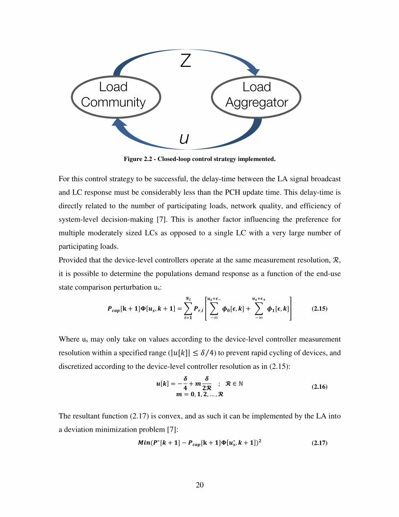
This control approach results in the closed-loop control strategy depicted in Figure 2.2[7].

20

Figure 2.2 - Closed-loop control strategy implemented.

For this control strategy to be successful, the delay-time between the LA signal broadcast

and LC response must be considerably less than the PCH update time. This delay-time is

directly related to the number of participating loads, network quality, and efficiency of

system-level decision-making [7]. This is another factor influencing the preference for

multiple moderately sized LCs as opposed to a single LC with a very large number of

participating loads.

Provided that the device-level controllers operate at the same measurement resolution, ℛ,

it is possible to determine the populations demand response as a function of the end-use

state comparison perturbation us:

8EW�Gp + JK[Ge�, H + JK = Y 8<,R]R

R^J i Y ZCGM, HKe��Mf�\ + Y ZJGM, HKe��Mb

�\ j (2.15)

Where us may only take on values according to the device-level controller measurement

resolution within a specified range (|GqK| ≤ r 4⁄ ) to prevent rapid cycling of devices, and

discretized according to the device-level controller resolution as in (2.15):

eGHK = − Tu + v TUw ; w ∈ ℕ v = C, J, U, … , w

(2.16)

The resultant function (2.17) is convex, and as such it can be implemented by the LA into

a deviation minimization problem [7]:

zR;(8∗GH + JK − 8EW�Gp + JK[Ge�∗, H + JK)U (2.17)

Load

Community

Load

Aggregator

Z

u

21

Where the optimal perturbation us* will result in an aggregate responsive load demand

equivalent to the specified target P*. To ensure the desired response of the aggregate

responsive load population is achieved, the specified target must exist within the feasible

region defined by:

�,+�Gq + 1K ≤ �∗Gq + 1K ≤ �,�|Gq + 1K �,�|Gq + 1K = ����Gq + 1KΦG,�|, q + 1K �,+�Gq + 1K = ����Gq + 1KΦG,+�, q + 1K

(2.18)

This feasible region defines the limitations of the VGM, corresponding to the virtual

generator ramp-rate at each time-step. As the load populations are dynamically evolving in

time, it is necessary to implement a closed-loop control strategy to ensure the LA can

accurately report the LCs capabilities as a VGM for each time-step.

2.5.2 Dispatch of multiple loads

The tracking error associated with multiple smaller LCs is found to be roughly equivalent

to the error associated with a single large LC containing the same total number of individual

loads [8]. This phenomenon, in conjunction with the need to maintain low computational

time of the system-level controller, provides incentive for a LA to distribute recruited loads

into multiple smaller VGMs rather than a single large model for each load type.

Furthermore, if a LA intends to manage different types of loads, it can reduce complexity

and improve system performance by developing individual VGMs for each type of load.

However, when operating multiple VGMs the LA must determine the optimal dispatch of

each VGM to achieve the global LA target response. It is preferable for the LA to minimize

the variability and magnitude of the end-use state comparison perturbation u [7].

Minimizing the magnitude of the perturbation serves to reduce the deflection from the

customers’ set-point values, and minimizing the variability of the perturbation accelerates

the dispersion of end-use states within the system-level equivalent deadband space. Greater

dispersion of end-use states results in a larger feasible space for the VGM, providing

additional flexibility in achieving the desired response of the power system operator.

By assuming that the amplitude of the control signal will be proportional to the amplitude

of the deflection of the LC from the uncontrolled trajectory, computational time can be

reduced by implementing a linear programming approach [7]. The uncontrolled trajectory

22

is equivalent to a trajectory with a perturbation of us[k] = 0, and also represents the lowest

variability and amplitude control signal possible:

8CGH + JK = 8EW�GH + JK[G(e� = C), H + JK (2.19)

Denoting the controlled deviation from P0 as ΔP*, and dropping the time-dependence, the

responsive load trajectory is given by:

8∗ = 8C + }8∗ (2.20)

The boundary conditions that govern the controlled deviation from the uncontrolled

trajectory are based on the maximum allowable set-point changes defined previously to

prevent rapid cycling of machines:

Δ�∗( = 0) = 0 Δ�∗( = r 4⁄ ) = �,�| − �/ Δ�∗( = − r 4⁄ ) = �/ − �,+�

(2.21)

Although the relationship between these boundary conditions may not be linear, a

reasonable first-order approximation is to assume the deflections in either direction are

proportional to the ratio of the controlled deflections and their maximums [7]:

= r4 Δ�∗�,�| − �/ �� > Y �/(�)��

�^0 = r4 Δ�∗�/ − �,+� �� < Y �/(�)��

�^0

(2.22)

Where PT is grid-side objective target for a LA dispatching Np responsive load communities

within the control area. The LA may then attempt to minimize control signal deflections,

while attempting to meet the grid-side objective target without violating any individual

VGM ramp constraints. Depending on the magnitude of the grid-side objective target, and

the aggregate uncontrolled trajectory of all participating loads, one of two linear

programming formulations are utilized:

23

�`� Y }8∗8vW�(�) − 8C(�)

]�

�^J�. �. Y }8∗(�) = 8@ − Y 8C(�)]�

�^J]�

�^J}8∗(�) ≤ 8vW�(�) − 8C(�)}8∗(�) ≥ C ∆8∗(�)8@ = 8vW�(�) − 8C(�)∑ (8vW�(�) − 8C(�))]��^J

(2.23)

When PT is greater than the aggregate uncontrolled trajectory, and:

�`� Y }8∗8C(�) − 8vR;(�)

]�

�^J�. �. Y }8∗(�) = 8@ − Y 8C(�)]�

�^J]�

�^J}8∗(�) ≤ 8C(�) − 8vR;(�)}8∗(�) ≥ C ∆8∗(�)8@ = 8C(�) − 8vR;(�)∑ (8C(�) − 8vR;(�) )]��^J

(2.24)

When PT is less than the aggregate uncontrolled trajectory.

Solving the linear programming formulation for the controlled deviations of each

population will ensure that the desired grid-side objective target can be attained, while

simultaneously minimizing the amplitude of the control signal u across each load-type. It

is imperative that the grid-side objective target is feasible for the participating LCs to

ensure a valid solution to the linear programming formulation is possible.

24

3 Computational Modeling Framework

This chapter describes the specific computational models that are employed to simulate the

various loads that comprise the load communities participating in the demand response

program.

3.1 Demand-side: Load Models

Demand-side load models must be capable of accurately simulating individual device

dynamics with minimal computational power. The following sections explain the dynamic

load models used to simulate the targeted end-use devices: Residential air-source heat

pumps, and plug-in electric vehicle charging.

3.1.1 Heat Pump Equivalent Thermodynamic Parameter Model

The study of building heating systems, such as air-source heat pumps, and their interactions

with building characteristics commonly results in the application of detailed multi-physics

approaches [7]. Due to the computational complexity of such simulations, they are not

suitable for modeling large populations of individual buildings as required for demand

response programs utilizing residential scale loads. A simplified model structure

commonly employed in such demand response simulations is the equivalent thermal

parameter (ETP) model [7], [8], [46].

The ETP model represents each building as a combination of thermal masses, which are

linked to one another via their related coefficients of heat transfer. Previous works have

employed a simple ETP model incorporating two coupled thermal masses to represent

small- to medium-sized buildings such as residential homes in North America [47]. This

coupled thermal system divides the home into two thermal masses: the thermal mass of the

air inside the dwelling Ca, and the thermal mass of the building structure Cm. These thermal

masses are then permitted to interact with the outdoor air temperature θa through the

building envelop thermal resistance Rao. The resulting temperature trajectories of the two

thermal masses are then coupled through the following linear dynamic system

representation:

25

� ����a� � = � � ���a� + � ����� � (3.1)

Where θm is the building contents temperature, and the system inputs are represented by

the outdoor air temperature θo, and the heat inputq� . The heat input used in this model is

based on the heating power of the heat pump�� ��, and the operational state of the heat pump

is determined by the hysteresis controller presented in section 2.4.3.

�� : ;�9��� ���9� (3.2)

The state- and input- transformation matrix, A and B, are determined from the structure of

the ETP, which is presented below in Figure 3.1 [7].

Figure 3.1 - ETP Schematic [7].

a00 : X � 1R��C� I 1R��C��a0� : 1R��C� a�0 : 1R��C� a�� : X 1R��C�

b00 : 1R��C� b0� : 1C� b�0 : 0b�� : 0 � : �a00 a0�a�0 a��� � : �b00 b0�b�0 b��� � : � ���a�   : ����� �

V� : ¡V I ¢£ (3.3)

A solution to the resultant discrete-time version of (3.3) under steady inputs is [48]:

VGH I JK : ¤VGHK I ¥£GHK Ω : exp�¡©�

Γ : A ¤¢ª«�/

(3.4)

Where Ω is the state-transition matrix, and Γ is the input-transition matrix. Because the

diurnal variations of outdoor temperature that affect device-level duty-cycles are much

longer than typical thermostat sampling frequencies, the utilization of temperature data

26

with a 1-minute resolution is reasonable [7]. Additional system internal gains and losses

(such as opening and closing doors, solar gains, air infiltration, and the operation of other

loads) are modeled with a white noise term, e, which is assumed to be normally distributed

with variance σ, and included in the component model utilized in this thesis according to

equation (3.5):

VGH I JK : ¤VGHK I ¥£GHK I PGHK (3.5)

3.1.1.1 Heat Pump Unit Sizing

To accurately model a representative population of homes, the heat pump unit sizing must

be suitable for the houses being simulated. To ensure reliability, the approach presented by

Parkinson was used for heat pump unit sizing [7]. This technique incorporates worst-case

scenario estimates of the parameters of the ETP model, in combination with the most

extreme environmental temperatures anticipated for the desired study area, to size heat

pumps for each modeled home. This is accomplished by balancing the heat flux from the

house that occurs under these conditions to maintain the indoor air temperature set-point

with the design heating power of the heat pump, and an appropriate oversizing factor. As

such, the design heating power of the heat pump can be determined using equation (3.6),

where γ is the over-sizing factor, θs is the thermostat set-point temperature, and θd is the

heating design temperature.

�� B : ¬ �V� X VB­W� � (3.6)

The variable efficiency of air-source heat pumps was addressed by fitting a third order

polynomial to the air-temperature efficiency curves from a manufacturer’s datasheet [49].

As a result, the power rating of individual units can be determined using the efficiency of

the heat pump at the design temperature, ηd:

8O : �� B%B (3.7)

From equation (3.7), the required electrical power to produce the design heating power is

Ph. This value was then rounded up to the nearest 0.5 kW to account for discretization

between units and conventional air-source heat pump availability [7], [49]. Under all but

the most extreme cold temperatures for the region, the heat pump will thus have excess

27

available capacity, and will cycle between the on and off states to maintain the indoor air

temperature according to equation (3.8).

�� O : %GHK8O (3.8)

A fan is used to circulate the heat produced by the heat pump throughout the building,

which also contributes to the operational capacity of the device. As a result, the operational

heat flux from the heat pump is the sum of the heat from the heat pump, and the additional

energy imparted by the operation of the fan.

�� ��GHK : �� OGHK I �� ®W; (3.9)

Assuming that the fan operates at an ideal efficiency, the total electric power associated

with the operational heat pump is then calculated by:

8< : 8O I 8®W; (3.10)

3.1.1.2 Heat Pump ETP Model Example

A simple example considering a single building is presented to demonstrate the device-

level dynamics of the ETP model. The parameters implemented in the model can be found

in [50] and [51], and are summarized below in Table 3.1 [7].

Table 3.1 - Parameters implemented in the heat pump ETP model.

Parameter Description Value

C Average thermal capacitance 10 kWh/°C

Cm Indoor contents thermal mass 75% of C

Ca Indoor air thermal mass 25% of C

Rma Indoor heat transfer resistance 0.5°C/kW

Rao Envelope thermal resistance 2°C/kW

�®W;� Heating power of fan 500 W

θs Temperature set point 20°C

δ Temperature deadband width 1°C

T Sampling time interval 1 minute

e Noise standard deviation 0.01°C s-1/2

28

The outdoor air temperature profile is shown in the top panel of Figure 3.2; the building

air- and contents-temperatures in the middle panel, and the device power requirements in

the bottom panel.

Figure 3.2 - Example of the ETP model response under the displayed outdoor temperature profile.

It is clear from this figure that the device cycles between on- and off-states in response to

the indoor air temperature traversing the deadband region. The transition of the building

air temperature through the deadband region is influenced by the outdoor air temperature,

traversing the deadband region more quickly during periods of colder temperatures.

3.1.2 Plug-in Electric Vehicle charging Model

The electrical demand associated with plug-in electric vehicle (PEV) charging is directly

related to the travel history of the vehicle, which can vary widely among potential users

due to a multitude of social factors. This large variance in travel history produces

significant variability in electric vehicle charging electrical demand, however once the

charging time and energy requirements are defined, a simple linear charging model can

identify real-time electrical demand for PEV charging. The three key parameters required

5

10

15

20

Ou

tdo

or

Tem

pera

ture

[°° °°C

]

17.5

18

18.5

19

19.5

20

20.5

Bu

ild

ing

Tem

pera

ture

[°° °°C

]

Air Thermal Mass Building Thermal Mass

00:00 03:00 06:00 09:00 12:00 15:00 18:00 21:00 00:00

0

2

4

6

8

10

12

Dem

an

d [

kW

]

Time of Day

29

for such a model are the desired battery charge capacity, the time that charging begins, and

the duration of time available before the desired battery charge capacity is required

(charging time).

By neglecting the travel history of the vehicle, and representing it simply as the required

battery charge capacity (which can be extrapolated to travel history), it is possible to model

the plug-in electric vehicle charging using a simplified linear model [7].

To determine the aggregate electrical load for a community of PEVs, a quasi-steady state

model of the charging reaction was implemented to simulate the device-level charging

controller. To account for the intrinsic heat loss to the environment during charging, a

defined charging efficiency, %, is employed. The resultant state-equation for the charging-

trajectory is thus:

?GH + JK = ?GHK + ;GHK%8<@ + PGHK (3.11)

Where the error term, e, is included to represent all un-modeled physical phenomena

(ambient temperature changes, transient electrochemical effects, etc.) and takes on a

magnitude of constant variance σ [7].

3.1.2.1 PEV Charging Model Example

A simple example considering the charging of a single plug-in electric vehicle is presented

to demonstrate the device-level dynamics of the EV charging model. The parameters

implemented in the model are based on average values from CPEVS survey data [52] and

previous work by Parkinson [7], as summarized in Table 3.2.

30

Table 3.2 - Parameters implemented in the EV charging model.

Parameter Description Value

Pr Rated power of the charger 5 kW

η Charging efficiency 0.95

Ec Desired charging capacity 11 kWh

Ts Desired charging duration 6 hours

δ Hysteresis control deadband 0.0025

T Sampling time interval 1 minute

e Noise standard deviation 0.01 kW

The hysteresis controller defined in section 2.4.3 provides device level control, resulting in

a duty-cycle-based charging rate and the resultant staggered charging trajectory [7]. The

selection of the device deadband width governs the duration of the active charging periods,

and with δ=0.025 in this example the operational periods last between about 20 and 30

minutes. The charging trajectory using the above parameters is shown in the top panel of

Figure 3.3. The middle panel shows the end-use state values of the hysteresis controller,

and the bottom panel shows the electrical demand from the charger.

Figure 3.3- Example of the EV load model.

0

5

10

Charg

ing

Tra

jecto

ry [kW

h]

e-

e+

End-u

se S

tate

Com

pari

son

Time of Day

19:00 20:00 21:00 22:00 23:00 00:00

0

2

4

6

Dem

and [kW

]

Time of Day

31

The PEV charging model also includes parameters to simulate vehicles joining and leaving

the load community, as well as access to daytime charging. Daytime charging is simulated

by creating a second ‘virtual’ PEV participant, with charging capacity equivalent to 50%

of the total charging capacity of the vehicle.

3.2 Supply-side: Power System Model

As one of the primary interests of this work is the compensation for the variability of wind

generation injected into the grid, a model to simulate wind generation is necessary. This

section introduces the modeling framework for wind energy generation and the basis for

calculation of wind generation from meteorological data.

3.2.1 Wind Energy Generation

Modern wind turbines are extremely complex machines, extracting energy from the wind

that passes over the turbines blades, producing lift which spins the turbine blades and in

turn an induction generator to generate electricity. Due to the large number of components,

and relative complexity of the wind generation system, it is generally preferable to develop

a simplified transfer function between wind speed input and power output [7].

In its simplest form, the transfer function is defined by a conversion from wind speed to

mechanical power imparted to the turbine hub, and a second conversion from the

mechanical power imparted to the turbine hub into useful electrical power. A quasi-steady

state function defining the mechanical power imparted to the wind turbine Pm as a function

of wind speed uw is given by [53]:

8v : J̄ °��±GHK, ²GHK�³´µUeQGHK¶ (3.12)

Where D is the rotor diameter, ρ is the air density, and Cp is the turbines coefficient of

performance as a function of tip-speed ratio λ and blade pitch angle β. A valid

approximation of Cp data, as used in previous works [7], [54], is the relation shown in

Equation.

32

°�GHK

:·̧̧¹¸̧º

C eQ < eER°�,v �J − »J � eveQGHK − J�U − »U � eveQGHK − J�¶� eER ≤ eQGHK ≤ e<°�,< � e<eQGHK�¶ e< ≤ eQGHK ≤ eE�C eQGHK > eE�

(3.13)

Where the turbine cut-in speed (uci) is the speed at which the turbine begins to generate

power, and the turbine cut-out speed (uco) is the speed at which the turbine furls and ceases

to generate power. Cp,m is the maximum turbine coefficient of performance, defined at the

wind speed um. The turbine rated speed, ur, is the speed at which Cp,r is defined by the

manufacturer. The coefficients F1 and F2 are derived from the boundary conditions, namely

Cp = 0 at uw = uci and Cp = Cr at uw = ur.

As in previous work by Parkinson, it is assumed that a gearbox with S stages is

implemented in the transmission of mechanical power to the electrical generator.

Consequently, the mechanical power available to the generator is further reduced by the

efficiency of the gearbox ηg[k] according to equation [55]. The piecewise equation is

necessary to ensure that the gearbox efficiency remains positive throughout the operating

regime of the wind turbine.

%¼GHK = ·¹º C. J 8vGHK ≤ ½8<9¾CJ − C. CJ½8<98vGHK �9OP<QR�P (3.14)

Where Prt is the rated power of the turbine at the rated wind speed, ur. Additional electrical

inefficiencies are not explicitly modeled, but are accounted for via the inclusion of an

additional electrical efficiency term ηe in the determination of electrical power provided to

the grid according to equation [7].

8¿GHK = %P%¼GHK8vGHK (3.15)

The input parameters used throughout this thesis for the wind generation model are

summarized in

Table 3.3, and are specified to represent a generic 1.5 MW system [7].

33

Table 3.3 - Parameters implemented in the wind energy system model [7].

Parameter Description Value

Prt Rated power of the turbine 1.5 MW

D Rotor diameter 82.5 m

uci Cut-in wind speed 4 m/s

uco Cut-out wind speed 26 m/s

ur Rated wind speed 12 m/s

Cp,r Rated coefficient of performance 0.250

Cp,m Maximum coefficient of performance 0.300

um Wind speed at Cp,m 7 m/s

S Number of stages in the gearbox 3

ηe Efficiency of the electrical components 0.95

Sample wind generation data is shown in Figure 3.4 based on NREL 80 m metrological

tower wind data for a one-day period [56].

Figure 3.4 - Sample wind speed data (top panel) and resultant model wind generation data (bottom

panel).

0

2

4

6

8

Win

d

Sp

eed

[m

/s]

00:00 06:00 12:00 18:00

0

200

400

600

Win

d

Po

wer

[kW

]

Time of Day

34

As one of the primary objectives of this thesis is to reduce the variance in the wind

generation injected into the grid, no consideration was given to the effects of multiple

turbines or distributed wind generation from multiple locations. Both of these effects

generally serve to reduce the variance of wind generation themselves, and thus ignoring

them represents a worst-case scenario.

3.3 Selecting the Simulation Time-step

The complete system model, incorporating each component model, requires the ability to

capture the dynamics of the load models and wind generation profile, while preserving the

accuracy of the system simulations. As in previous works on demand response [7], [8], a

one-minute sampling time (T = 1 min) provides sufficient accuracy while permitting

transient population dynamics to dissipate. This time-step also permits participation in

ancillary service markets such as regulating reserve; services that generally take place on

intervals of 5 to 15 minutes [7], [20]. Further, a smaller sampling time could introduce

error, as it has been shown that below 1 minute generation does not exactly follow the load

[48].

In addition, the 1 minute time step also permits loads to freely enter into and leave the load

community – this is particularly important for PEV charging, as users can freely leave the

demand response population with minimal impact on overall system performance [7].

Further, the device level controller may not be compatible with longer simulation time-

steps and aliasing errors could arise. For these reasons, a 1 minute time-step was selected

for all simulations in this thesis.

35

4 Demand Response Algorithms

The algorithms presented in section 2.5 are now adapted to account for limited reporting

of device-state information by a subset of the total participating population of loads in the

DR program. The underlying hysteresis control structure is unchanged, however the system

response must be calculated based on a limited number of devices reporting device-state

information.

4.1 Accounting for Limited Knowledge of Load States

When only a subset of the total participating population is reporting device-state

information, the determination of the population capacity factor, and resultant system

response must be modified from the algorithms presented in section 2.5. The capacity

factor under these limited information scenarios must be determined from only the

reporting loads, according to equation (4.1):

[�RvR9PBGe�, H I JK : Y ZC,<GM, HKe��Mf

�\I Y ZJ,<GM, HKe��Mb

�\ (4.1)

The capacity factor determined from device-state information of the reporting loads is then

multiplied by the total capacity of the population, including loads that are participating in

the DR program but do not report state-information. The resultant response of the system

can be determined by equation (4.2):

8EW�Gp I JK[�RvR9PBGe�, H I JK : 8EW�GH I JK Y ZC,<GM, HKe��Mf

�\I Y ZJ,<GM, HKe��Mb

�\ (4.2)

The underlying assumption with this control algorithm is that the sampled subset of the

total population is representative of the whole population. The VGM limits under limited

knowledge scenarios must also be calculated based on the subset of the population

reporting device-state information, according to equation (4.3):

�,+�Gq I 1K = Φ*+,+-'�G,+�, q + 1K����Gq + 1K �,�|Gq + 1K = Φ*+,+-'�G,�| , q + 1K����Gq + 1K (4.3)

36

These calculations once again rely on the assumption that the sampled subset of loads

reporting device-state information is representative of the total population. Further

refinement of this control algorithm under limited device-state information are possible by

sampling the actual population response and comparing it with the expected response based

on equation (4.3). In this manner, a correction factor could be applied to subsequent time-

step calculations to reduce the error between anticipated and actual DR population

response.

4.2 Control Performance Metrics

The power tracking performance at each one-minute time step was tracked throughout

simulations to determine controller performance. To ensure consistent results across all

scenarios tested, the systems were initialized at approximately steady state conditions. Two

metrics were used in the evaluation of system performance: 1) The root mean squared

power tracking error, and 2) The load flexibility and under-utilization factor. These

evaluation criteria are explained in detail below.

4.2.1 RMS Error %

The Root mean squared power tracking error (RMSE) is calculated for the duration of the

simulation under consideration according to equation (4.4):

­z½? = À∑ (8WE9eW� − 89W<¼P9)UÁH^J Á (4.4)

The RMSE is then normalized with respect to the steady state power consumption of the

population as shown below

]­z½? = ­z½?vPW;(8C) (4.5)

This metric allows the comparison of various scenarios relative to a standard baseline, and

has been used in previous demand response work as a performance criteria [8].

37

4.2.2 Load Flexibility/Under-Utilization Factor

In addition to the power tracking performance of the system, it is important to determine

the load community flexibility and the un-utilized capacity at each time step. Load

flexibility is calculated according to equation (4.6), and is analogous to the generator ramp

rate of conventional generation resources [7]. Due to the nature of the load community, the

load flexibility or ramp-rate is essentially equivalent to the available capacity of the system.

Â(�)GHK = 8vW�(�) GHK − 8vR;(�) GHK (4.6)

In addition, a measure of the available excess capacity available in each load community

for each time step was also calculated. Both up- and down-regulation capacity are evaluated

separately, resulting in two under-utilization factors for each time-step. These values are

calculated according to equation:

ÃB�Q;GHKÃe�GHK = a`� ((8vW�GHK − 8CGHK), (8vW�GHK − 8WE9eW�GHK))a`� ((8CGHK − 8vR;GHK), (8WE9eW�GHK − 8vR;GHK)) (4.7)

where Pactual is the measured power dispatched from the load community for each time step,

P0 is the steady-state power required by the load community, Pmin is the minimum feasible

target power of the load community, and Pmax the maximum feasible target power of the

load community. The minimization operator ensures that actual dispatched capacity is not

considered part of the un-utilized capacity available. It is important to note that due to the

dynamic nature of the simulations, usage of the un-utilized capacity from one time step

will inherently affect the load community for subsequent load steps – however it is a valid

measurement of the utilization of the load for offline review. Finally, the total energy

dispatched from each VGM population is determined according to:

?µ(�) = YÄ∆8(�)GHKÄ@]HH^J (4.8)

Where up- and down-regulation dispatched are considered equivalent contributions to total

energy dispatched by a VGM model.

38

4.3 Model Input Data

The validity of model input data can greatly influence the results of simulations, thus real

world historical datasets relevant to the proposed simulation scenarios were employed. As

in previous work [7], the recruited load communities are intended to be representative of a

suburban or rural community connected to a single distribution system, or approximately

2000 customers [58]. For the purposes of this thesis, it was assumed that initial populations

of 1500 heat pumps and 1500 PEVs could be recruited from this community [7].

To ensure a realistic representation of the loads, populations were intentionally generated

to be heterogeneous – this will ensure that the device diversity expected in typical

communities is represented. This heterogeneity is achieved by selecting normally

distributed values for the individual component models based on representative data for

each of the populations under consideration.

4.3.1 Environmental Data - Air Temperature & Wind Speed

Outdoor air temperature and wind speed data were obtained from the National Renewable

Energy Laboratory (NREL) database. Specifically, data was obtained from the National

Wind Technology Centre M2 Tower, located about 11 km west of Broomfield, and 8 km

south of Boulder, Colorado (Latitude: 39° 54' 38.34" North; Longitude: 105° 14' 5.28"

West; Elevation: 1855 meters AMSL).

Air temperature measurements are taken at 2m elevation, while wind speed measurements

are taken at 80 m elevation. Sample air temperature and wind speed data are shown in

Figure 4.1, representing a 24 hour period beginning August 1, 2014 [56].

Figure 4.1 - Representative outdoor air temperature and wind speed data from NWTC M2 tower.

00:00 03:00 06:00 09:00 12:00 15:00 18:00 21:00 00:000

2

4

6

8

10

12

14

Time of Day

Air Temperature [°C] Wind Speed [m/s]

39

In this thesis environmental datasets were selected for the period of October 2013, as this

represents a moderate heating demand on the heat pumps, without the requirement to also

model cooling loads. During periods of cooler weather, home air temperatures will traverse

the deadband region more rapidly than during periods of warmer weather, resulting in

greater availability to participate in the demand response program.

4.3.2 Thermodynamic Data - Heat Pump Sizing and ETP Values

For the purposes of simulations in this thesis, parameters used in the ETP model were

selected to represent typical single-family homes in the Pacific Northwest. While work is

currently ongoing to determine specific ETP parameters to represent a wide variety of

buildings [47], there are a number of works that employ the ETP model to represent average

homes in the Pacific Northwest [7], [46], and [59].

The ETP model parameters utilized throughout this thesis are summarized in Table 4.1

[59].

Table 4.1 - ETP Model Input Parameters.

Parameter Description Value

C Average thermal capacitance 10 kWh/°C

Cm Indoor contents thermal mass 75% of C

Ca Indoor air thermal mass 25% of C

Rma Indoor heat transfer resistance 0.5°C/kW

Rao Envelope thermal resistance 2°C/kW �®W;� Heating power of fan 500 W

θs Temperature set point 20°C

δ Temperature deadband width 1°C

T Sampling time interval 1 minute

σ Noise standard deviation 0.01°C s-1/2

σp Standard deviation of lognormal distributions as a fraction of the mean value, for R, C, and P, unless noted otherwise

0.2

40

Load community populations were then derived from this data by selecting lognormal

distributed values from this data, resulting in a homogenous load community as shown in

Figure 4.2. Lognormal distributions were chosen primarily to ensure that all parameters

remain positive Figure 4.2.

Figure 4.2 - Scatterplot showing selected ETP parameters for a population of 1500 heat pumps.

4.3.3 PEV Data - Vehicle Sizing & Charging Schedules

Previous work incorporating Plug-in Electric Vehicle (PEV) charging loads have generally

relied upon estimates of charging schedules and parameters [7]. To increase the accuracy

of the PEV load community, results from a survey conducted by SFU of personal driving

habits and PEV integration were used to create representative load communities. Survey

data included detailed driving parameters of 1754 individuals across Canada, with 538

respondents from BC [52]. Based on this survey data, it was possible to derive the

distributions of the parameters required for the PEV charging models employed in this

thesis – Specifically the charging start time, charging duration, and required charge

5 10 15 20 256

7

8

9

10

11

12

13

14

15

16

Heat Pump Power Rating [kW]

Bu

ild

ing

Heat

Cap

acit

y [

kW

h/

°° °°C

]

41

capacity of the vehicle, as summarized in Table 4.2. The rated power of chargers was

specified such that the population had an average value of 5 kW, with a standard deviation

of 0.5 kW, which are representative of widely available Level 1 chargers.

Table 4.2 - PEV Charging Model Input Parameter Distribution Data

Parameter Description Average Value Standard Deviation

Tstart Charging start time 17:10 hrs. 235 minutes

Ts Desired time to accumulate Ec 1018 minutes 313 minutes

Pr Rated power of charger 5 kW 0.5 kW

Ec Desired charging capacity 11.3 kWh 2 kWh

Statistical analysis of the survey data showed that the correlation coefficients among

charging start time, charging duration, and required charge capacity were all less than 0.1,

indicating weak- or no-correlation. As a result, populations of plug-in electric vehicles were

generated by selecting random values from these normal distributions. The distribution of

charging start and end times from a sample population of 1500 Plug-in electric vehicles is

shown in Figure 4.3.

Figure 4.3 - Scatterplot showing PEV charging start and end times.

0 200 400 600 800 1000 1200 14000

200

400

600

800

1000

1200

1400

EV Charging Start Time [mins]

EV

Ch

arg

ing

En

d T

ime [

min

s]

42

It is evident from Figure 4.3 that there are two predominant charging windows – the

daytime charging window, indicated by the upper diagonal cluster of points, and overnight

charging, as indicated by the lower diagonal cluster of points. Further, the availability of

daytime charging access was included in the survey data, which was extrapolated to

determine the proportion of the population that would have access to daytime charging as

shown in Figure 4.4 [52].

Figure 4.4 - Recharge access by time of day (BC only, n=528, 3-day driving diary) [52].

Approximately 30% of survey respondents had some form of access to charging stations

throughout the day, which forms the basis for the percentage of individual loads permitted

daytime charging in simulations throughout this thesis.

4.3.4 Target Trajectory

The control algorithms implemented in this thesis are designed to dispatch the participating

load communities to meet an externally specified target trajectory provided to the load

aggregator. However, if the specified target trajectory exceeds the capabilities of the

participating load communities, the target trajectory will be truncated to achieve the largest

response possible given the current state of the load communities according to equation

(4.9):

43

8@ : Å8vR; 8@ < 8vR;8vW� 8@ > 8vW�8@ P��P (4.9)

Where Pmin and Pmax are determined based on the maximum permitted control signal

magnitude δ/4, previously defined in section 2.5.1.

In scenarios with limited knowledge, however, the value of the capacity factor is calculated

based only on the reporting loads. The population is split into two categories: reporting

loads (inactive-state, ϕ0,r and active-state ϕ1,r), and participating loads. Under these limited

knowledge scenarios, the calculation of Pcap is the same as the full knowledge scenarios;

however the calculation of the capacity factor is based solely on the reporting loads:

[�RvR9PBGe�, H I JK : Y ZC,<GM, HK}Me��Mf

�\I Y ZJ,<GM, HK}Me��Mb

�\

�,�| : ����Gq I 1KΦ*+,+-'�Gr4 , q + 1K �,+� = ����Gq + 1KΦ*+,+-'�G− r4 , q + 1K

(4.10)

A target trajectory for the participating loads is thus defined as:

8∗GHK = @W<¼P9GHK + Y 8C(�)GHK]�

�^J (4.11)

This aggregate participating load target, P* must fall within the range of feasible targets

8vR; ≤ 8∗ ≤ 8vW� (4.12)

If the aggregate participating load target falls outside of this range, the controller truncates

the load target to either the maximum of minimum value that can be achieved by the

populations.

In this thesis, two target load trajectories are implemented: a regulating reserve dispatch

signal from a utility operator, and a self-generating signal to reduce the variability of wind

generation from a wind turbine. These target trajectories are described in detail in the

following sections.

44

4.3.4.1 Regulating Reserve Dispatch Signal

In order to test the demand response system to provide regulating reserve ancillary services

to the power systems operator, a target trajectory was specified based on historical

regulating reserve capacity dispatched in the BPA balancing authority area [19], as shown

in Figure 4.5.

Figure 4.5 - BPA Balancing Reserves Available & Dispatched July 31 - Aug 7, 2014 [19]

The target trajectory was then generated by scaling the balancing reserves dispatched

values for a 24-hour simulation period, and inverting the sign to ensure a request for

generation results in a decrease in demand. As this portion of the balancing reserves are

then served by the demand response program, the resultant balancing reserves required by

the balancing area to be supplied from conventional generation resources will be reduced.

The frequency distributions of one year’s worth of BPA balancing reserves dispatched data

is shown below in panel 1 of Figure 4.6, which closely resembles the frequency distribution

of the 24-hour simulation period balancing reserves deployed used as a basis for the target

trajectory for simulations in this thesis.

31-Jul-2014 01-Aug-2014 02-Aug-2014 03-Aug-2014 04-Aug-2014 05-Aug-2014 06-Aug-2014

-1000

-500

0

500

1000

MW

Date

Balancing Reserves Incremental Reserves Available Decremental Reserves Available

45

Figure 4.6 - Frequency distribution of BPA balancing reserves dispatched data from 2014 (left panel)

and 24-hour simulation period (right panel).

The similarities among the frequency distributions of the data for balancing reserves

dispatched in Figure 4.6 shows that the 24-hour simulation window is representative of

annual balancing reserves dispatched. The target trajectory was scaled down to 0.5% of the

total balancing reserves dispatched in the BPA network, to ensure that it was within the

feasible region for populations of 1500 homes and 1500 EVs.

4.3.4.2 Reducing Variability of Wind Generation Target Signal

As described in section 3.2.1, wind energy generation exhibits considerable variability at a

one-minute resolution time-step, especially when considering an individual wind turbine

or single wind farm. It is possible to utilize demand response programs to modify the

demand curve in response to variations in wind generation, thus resulting in a significant

reduction in variability to the net power required from the electrical grid. For the purposes

of this thesis, a target trajectory to smooth wind generation injections from a single 1.5

MW wind turbine is employed. The target trajectory attempts to the net power injections

into the grid according to the 15 minute moving average wind generation profile according

to equation (4.13):

@W<¼P9GH I JK : 8QR;B,JÆ a`� WǼGHK X 8QR;B,WE9eW�GH I JK (4.13)

-1500 -1000 -500 0 500 1000 15000

100

200

300

400

500

600

frequency

Power [MW]

2014 Balancing Reserves Deployed

-1500 -1000 -500 0 500 1000 15000

5

10

15

20

25

30

35

40

45

frequency

Power [MW]

24-hr Simulation Period Balancing Reserves Deployed

46

Where the 15 minute moving average is calculated according to equation (4.14):

8QR;B,JÆ a`� WǼGHK : JJÆ Y 8QR;B,WE9eW�GH I vKCv^�JÆ

(4.14)

This target trajectory assumes that the next time-step wind generation is known, however

this is not an unreasonable assumption given the accuracy of conventional persistence

modeling and advanced meteorological modeling [59]. A target trajectory based on sample

wind speed data is shown in Figure 4.7.

Figure 4.7 - Sample target trajectory and net grid power injections based on wind generation profile

from section 3.2.1.

As shown in Figure 4.7, the demand response target will always supply the difference in

generation at each time step from the 15 minute moving average, smoothing the net impact

of variable generation injected into the grid. Figure 4.8 shows the frequency distribution of

wind speed at the NREL meteorological tower [56] for the past year (left panel), and for

the 24-hour simulation period under consideration (right panel)

00:00 00:00

-2000

-1500

-1000

-500

0

500

1000

1500

2000

2500

Po

wer

[kW

]

Time of Day

Wind Generation Profile Target Trajectory Net Grid Injection

47

Figure 4.8 - Frequency distribution data for NREL wind speed data from 2014 (left panel) and 24-

hour simulation period (right panel).

While seasonal variations will exist with respect to wind speed data and the resultant wind

generation injections into the grid, the 24 hour sample period provides a representative

sample of the major short-term variability to be expected from a demand response program

operating to smooth wind energy generation injections. The target trajectory was specified

to simulate smoothing the power injections to the grid from a 3 MW wind turbine to ensure

that it always remains in the VGM feasible regions for 1500 Homes and 1500 EVs.

0 5 10 150

5

10

15

20

25

30

35

40

45

50

frequency

Wind Speed [m/s]

2014 Wind Speed

0 5 10 150

5

10

15

frequency

Wind Speed [m/s]

24-hr Simulation Period Wind Speed

48

5 Model Results

This section will present simulation results, initial analysis of the VGM population

dynamics, and draw conclusions with respect to the observed performance of the proposed

demand response system. In all scenarios, simulations were run for a 2-day period (2881

minutes). The first 24-hours (1440 minutes) of the simulation results were discarded to

ensure any transient response from initializing the demand response program did not affect

the results of the simulations, and all analysis was conducted on the data from the remaining

24-hour simulation period.

5.1 Provision of Wind-Generation Smoothing Services

A second scenario was considered for the demand response system, utilizing the VGMs to

smooth wind generation injections into the electrical grid. Historically, increased

penetration of wind generation into the electrical grid has necessitated additional

dispatchable power capacity to firm-up the variable power injections from wind generation

[12]. In the wind-firming scenario, rather than relying on conventional dispatchable

generation to firm wind power injections, demand response populations are utilized to

adjust demand in real-time in response to variations in wind power generation. In this

scenario, the target trajectory is specified according to the procedure indicated in section

4.3.4.2, and shown in Figure 5.1.

Figure 5.1 - Wind Generation Smoothing Target Trajectory

00:00 03:00 06:00 09:00 12:00 15:00 18:00 21:00 00:00-3000

-2000

-1000

0

1000

2000

3000

4000

5000

Simulation time [mins]

Pow

er

[kW

]

Target Trajectory Maximum Aggregate Load Available Minimum Aggregate Load Available

49

This target trajectory results in a net injection to the electrical grid equivalent to the 30-

minute moving average of the wind generation values, rather than the highly variable real-

time wind generation profile shown in Figure 5.2.

Figure 5.2 - Wind Generation over 24-hour Simulation Period.

As a result, the variability of power injections into the grid are greatly reduced, reducing

the requirements for conventional dispatchable generating resources to provide balancing

reserves. Once again, 1500 heat pumps and 1500 EVs were selected for this scenario, and

the wind farm capacity was scaled such that the target trajectory remains within the feasible

region throughout the simulation period, as shown in Figure 5.1.

Again, the resultant VGM response is within 2% of the target trajectory, primarily

attributed to discretization of the deadband region and quantized device-level power

ratings. The resultant controlled and uncontrolled trajectories of each VGM, and the

cumulative population trajectory are shown in Figure 5.3.

00:00 03:00 06:00 09:00 12:00 15:00 18:00 21:00 00:000

500

1000

1500

2000

2500

3000

Simulation time [mins]

Win

d G

en

era

tio

n [

kW

]

50

Figure 5.3 - Demand Response System trajectories.

Similarly to the scenario providing ancillary services in the previous section of this thesis,

the Heat Pump VGM exhibits greater flexibility, once again owing to the transient nature

of EV Charging vehicles connecting to and disconnecting from the system throughout the

day. The individual VGM flexibilities and under-utilized capacities are shown in Figure

5.4.

2000

4000

6000

8000H

eat

Pu

mp

s

Po

wer

[kW

]

Target Response Actual Response Min Boundary Max Boundary

0

1000

2000

3000

EV

s C

harg

ing

Po

wer

[kW

]

06:40 06:50 07:00 07:10 07:20 07:300

2000

4000

6000

8000

10000

To

tal

Lo

ad

[kW

]

Time of Day

51

Figure 5.4 - Individual VGM flexibility and under-utilization factors.

Power density distributions for each of the VGMs are also similar under the wind-firming

scenario as they are in the regulation reserve scenario, as shown in Figure 5.5.

Figure 5.5 - Density plots of VGMs.

0

2000

4000

6000V

GM

Fle

xib

ilit

y [

kW

]

Heat Pumps EV Charging

0

1000

2000

3000

4000

Decre

men

tal

Cap

acit

y [

kW

]

00:00 03:00 06:00 09:00 12:00 15:00 18:00 21:000

1000

2000

Incre

men

tal

Cap

acit

y [

kW

]

Time of Day

10

20

30

40

50

60

Heat

Pu

mp

s -

In

acti

ve S

tate

e-

0

e+

Heat

Pu

mp

s -

Acti

ve S

tate

e-

0

e+

EV

Ch

arg

ing

- I

nacti

ve S

tate

Time of Day

06:30 06:45 07:00 07:15

e-

0

e+

EV

Ch

arg

ing

- A

cti

ve S

tate

Time of Day

06:30 06:45 07:00 07:15

e-

0

e+

Power [kW] Uncontrolled State-Transition Boundary Controlled State-Transition Boundary

52

Large magnitude control signals result in synchronization of loads within each of the

VGMs, however this load synchronization rapidly dissipates naturally throughout the

populations due to the heterogeneous populations modeled.

Again, owing to the larger available capacity of the Heat Pump VGM compared to the EV

charging VGM, the Heat Pump VGM dispatched almost twice the energy throughout the

simulation period, as shown in Table 5.1.

Table 5.1 - Performance of Load Resources Performing Wind Smoothing Services.

Load Type Dispatched

Energy

[MWh]

Mean VGM

Flexibility

[MW]

Mean Control Signal

Magnitude

[% of umax]

Control Signal

Standard Deviation

[% of umax]

Heat Pumps 6.04 4.35 0.43 20.49

EV Charging 0.182 1.186 0.68 3.30

The magnitude of the mean control signal for both populations was very small, primarily

due to the large variations in wind generation power over short time periods, coupled with

extended periods of zero wind generation. As the target trajectory was scaled to ensure it

was always within the feasible region of the VGMs, the utilization of the VGMs during

non-peak target trajectory periods is rather low. If conventional balancing resources were

utilized to cover the large spikes in target trajectory, a much larger amount of energy could

be dispatched from the demand response program. It would thus be possible to employ the

demand response system to provide additional services concurrently with wind-generation

smoothing during the periods of zero or low wind generation.

5.1.1 Limited-knowledge Population Dynamics

In order to test the effects of limited knowledge on the demand response system, and the

individual VGM population dynamics, eleven additional scenarios were considered with

progressively less device state information. Simulations were conducted with reduced

knowledge, ranging from 100% knowledge to 20% knowledge, to determine the effects on

overall system response when providing wind generation firming services using the same

target trajectory as shown in Figure 5.1. The overall load trajectories of these simulations,

53

as well as the actual system response under various limited device-state information

scenarios are shown in Figure 5.6.

Figure 5.6 - System response and Target trajectory under limited-knowledge simulations.

As shown in Figure 5.7, the error associated with the VGM response increases as device-

state information is decreased, as would be expected. However, even at very low state-

information levels the normalized root mean squared error associated with the demand

response system remains below 10%. Once again, this error is largely attributed to

discretization of the deadband region, and quantized device-level power ratings; although

the reduced information scenarios amplifies these effects noticeably.

-2000

-1500

-1000

-500

0

500

1000

Target 100% 90% 80%

-2000

-1000

0

1000

2000

Pow

er

[kW

]

Target 70% 60% 50%

06:20 06:30 06:40 06:50 07:00 07:10-2000

-1000

0

1000

2000

Time of Day

Target 40% 30% 20%

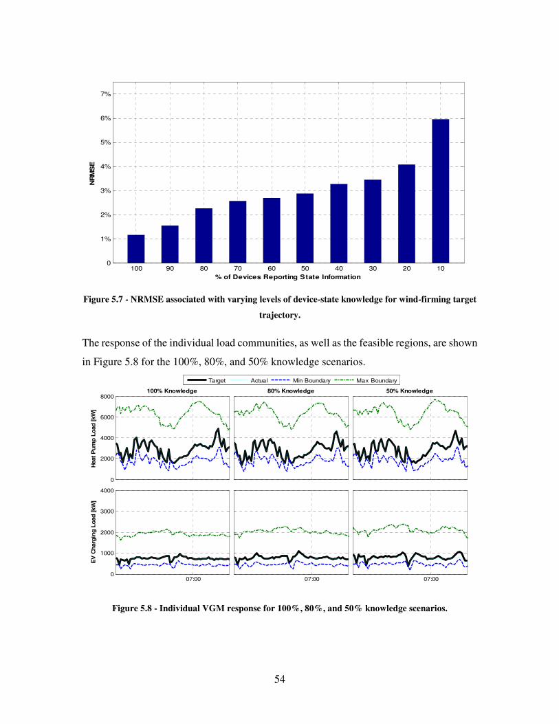
54

Figure 5.7 - NRMSE associated with varying levels of device-state knowledge for wind-firming target

trajectory.

The response of the individual load communities, as well as the feasible regions, are shown

in Figure 5.8 for the 100%, 80%, and 50% knowledge scenarios.

Figure 5.8 - Individual VGM response for 100%, 80%, and 50% knowledge scenarios.

100 90 80 70 60 50 40 30 20 100

1%

2%

3%

4%

5%

6%

7%

% of Devices Reporting State Information

NR

MS

E

0

2000

4000

6000

8000100% Knowledge

Heat

Pum

p L

oad

[kW

]

80% Knowledge 50% Knowledge

07:0007:000

1000

2000

3000

4000

EV

Charg

ing L

oad [kW

]

07:00

Target Actual Min Boundary Max Boundary

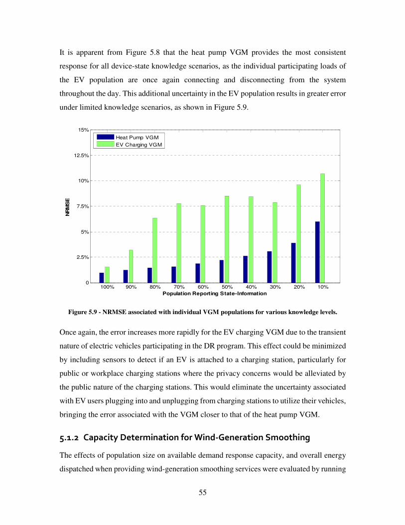
55

It is apparent from Figure 5.8 that the heat pump VGM provides the most consistent

response for all device-state knowledge scenarios, as the individual participating loads of

the EV population are once again connecting and disconnecting from the system

throughout the day. This additional uncertainty in the EV population results in greater error

under limited knowledge scenarios, as shown in Figure 5.9.

Figure 5.9 - NRMSE associated with individual VGM populations for various knowledge levels.

Once again, the error increases more rapidly for the EV charging VGM due to the transient

nature of electric vehicles participating in the DR program. This effect could be minimized

by including sensors to detect if an EV is attached to a charging station, particularly for

public or workplace charging stations where the privacy concerns would be alleviated by

the public nature of the charging stations. This would eliminate the uncertainty associated

with EV users plugging into and unplugging from charging stations to utilize their vehicles,

bringing the error associated with the VGM closer to that of the heat pump VGM.

5.1.2 Capacity Determination for Wind-Generation Smoothing

The effects of population size on available demand response capacity, and overall energy

dispatched when providing wind-generation smoothing services were evaluated by running

100% 90% 80% 70% 60% 50% 40% 30% 20% 10%0

2.5%

5%

7.5%

10%

12.5%

15%

Population Reporting State-Information

NR

MS

E

Heat Pump VGM

EV Charging VGM

56

simulations of populations ranging in size from 500 devices to 6000 devices.

Heterogeneous populations of equal numbers of heat pumps and EV charging loads were

paired with iteratively scaled target trajectories to ensure that the populations were never

over-dispatched. Simulations of each population size (500, 1000, 1500, 3000, 4500, and

6000) were conducted under 100% knowledge scenarios, and the resultant mean VGM

capacities and net energy dispatched was evaluated. Figure 5.10 shows the energy

dispatched by the DR program for various population sizes, as well as the mean available

capacity of the VGMs of varying sizes.

Figure 5.10 - Energy Dispatched by VGMs (top panel) and Mean Available VGM Capacity (bottom

panel) for Various Load Community Population Sizes.

As the population size of the VGMs is increased, the dispatched energy from the DR

program increases proportionally. In addition, the available mean capacity of the DR

program increases proportionally with the population size. Each VGM responds similarly,

with the heat pump VGM remaining the largest contribution to the demand response

program in these scenarios.

0

0.5

1

1.5

2

2.5x 10

4

To

tal

En

erg

y

Dis

patc

hed

[kW

h]

Heat Pumps EV Charging

500 1000 1500 3000 4500 60000

0.5

1

1.5

2

2.5x 10

4

Mean

Avail

ab

le

Cap

acit

y [

kW

]

Load Community Population Size [# Units]

Heat Pumps EV Charging

57

The effects of scaling population sizes on the available mean capacity would be useful for

utility systems operators to determine how many responsive loads they would need to

recruit to achieve a desired capacity from the DR program. In all scenarios, the mean

control signal magnitude and the control signal standard deviation remained within 1% of

one another, and within 2% of one another, respectively. This implies that the

inconvenience of the DR program on end-user functionality is not significantly affected by

VGM population size.

5.2 Provision of Regulating Reserve Ancillary Services

To simulate the provision of balancing reserve ancillary services to a power systems

operator, a target trajectory corresponding to the BPA historical balancing reserves

dispatch history was created as described in section 4.3.4.1. This target trajectory was then

iteratively scaled to a point where it remains entirely within the feasible region of the VGM

of home heat pumps and PEV charging, as shown in Figure 5.11. This scaled trajectory

represents 0.5% of the total balancing reserves dispatched by the BPA over a 24-hour

period [19].

Figure 5.11 - Scaled target trajectory & VGM feasible region boundaries.

00:00 06:00 12:00 18:00 00:00-3000

-2000

-1000

0

1000

2000

3000

4000

5000

Simulation time [mins]

Pow

er

[kW

]

Target Trajectory Maximum Aggregate Load Available Minimum Aggregate Load Available

58

Heat pump and PEV charging populations were selected to represent a small suburban or

rural community connected to a single distribution system, resulting in populations of 1500

heat pumps and 1500 PEVs [58]. To represent the diversity of real-world populations, heat

pump and PEV charging parameters were drawn from normal distributions of parameters

as described in the previous sections.

With the model inputs defined, two preliminary scenarios were considered: The first,

without any intervention by the demand response system to represent the uncontrolled

trajectory of the load populations; and the second with the demand response system applied

under the assumption of full device-state knowledge. The resultant load trajectories under

both scenarios, as well as the individual VGM responses, are shown in Figure 5.12.

Figure 5.12 - Uncontrolled and Controlled Population Response.

The controlled scenario follows the target trajectory specified, resulting in less than 2%

NRMSE throughout the simulation period. The heat pump loads provide greater demand

response capacity than the PEV charging loads due to the fact that the heat pumps are

available throughout the entire 24 hour period, while PEV charging loads enter and leave

the demand response program as they are utilized by owners for transportation. Detailed

1000

2000

3000

4000

5000

Heat

Pu

mp

Lo

ad

[kW

]

Uncontrolled Controlled

0

500

1000

1500

2000

2500

EV

Ch

arg

ing

Lo

ad

[kW

]

00:00 06:00 12:00 18:00 00:00

2000

4000

6000

To

tal

Lo

ad

[kW

]

Time of Day

59

plots showing the individual VGM responses, as well as the feasible region, are shown in

Figure 5.13

Figure 5.13 - Individual VGM Feasible Regions, Target Trajectory, and Actual Response.

The maximum and minimum boundaries define the largest magnitude response that the

VGM is capable of providing to the system at each time step, and changes throughout the

simulation period in response to utilization of the demand response resource. As a result,

the specified target trajectory must remain within these boundaries throughout the demand

response program operation to ensure the desired response from the system is feasible.

The flexibility and the under-utilization factors of the VGMs, as described in section 4.2.2,

are shown below in Figure 5.14.

0

2000

4000

6000

8000

Heat

Pu

mp

s

Pow

er

[kW

]

Target Response Actual Response Min Boundary Max Boundary

0

1000

2000

3000

EV

s C

harg

ing

Po

wer

[kW

]

18:30 18:45 19:00 19:150

5000

10000

Tota

l

Lo

ad [

kW

]

Time of Day

60

Figure 5.14 - VGM Flexibility and under-utilization factors.

This represents the maximum feasible region within which demand response services are

achievable for the VGMs, as well as the effective ramp-rate that each VGM is capable of

achieving in the next time-step. It is important to note that the feasible region is constantly

evolving in response to the dispatched power from previous time-steps as devices transit

the deadband region and replenish the population flexibility. There are a few instances

throughout the simulation period where the incremental capacity of the VGMs approaches

saturation, however these regions of saturation rapidly replenish when the output demanded

of the VGMs is reduced. This can clearly be seen in Figure 5.14 above for the Heat Pump

VGM between the hours of 22:30 and 23:30. The resultant power density distributions of

all devices within the VGM are shown in Figure 5.15.

2000

4000

6000V

GM

Fle

xib

ility [kW

]

Heat Pumps EV Charging

0

1000

2000

3000

4000

Decre

menta

l

Cap

acit

y [kW

]

19:00 20:00 21:00 22:00 23:000

500

1000

1500

2000

Incre

men

tal

Capacity [kW

]

Time of Day

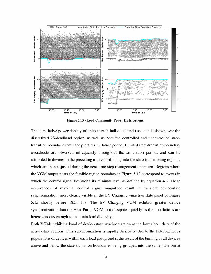
61

Figure 5.15 - Load Community Power Distributions.

The cumulative power density of units at each individual end-use state is shown over the

discretized 2δ-deadband region, as well as both the controlled and uncontrolled state-

transition boundaries over the plotted simulation period. Limited state-transition boundary

overshoots are observed infrequently throughout the simulation period, and can be

attributed to devices in the preceding interval diffusing into the state-transitioning regions,

which are then adjusted during the next time-step management operation. Regions where

the VGM output nears the feasible region boundary in Figure 5.13 correspond to events in

which the control signal lies along its minimal level as defined by equation 4.3. These

occurrences of maximal control signal magnitude result in transient device-state

synchronization, most clearly visible in the EV Charging –inactive state panel of Figure

5.15 shortly before 18:30 hrs. The EV Charging VGM exhibits greater device

synchronization than the Heat Pump VGM, but dissipates quickly as the populations are

heterogeneous enough to maintain load diversity.

Both VGMs exhibit a band of device-state synchronization at the lower boundary of the

active-state regions. This synchronization is rapidly dissipated due to the heterogeneous

populations of devices within each load group, and is the result of the binning of all devices

above and below the state-transition boundaries being grouped into the same state-bin at

10

20

30

40

50

60H

eat

Pu

mp

s -

In

acti

ve S

tate

e-

0

e+

Heat

Pu

mp

s -

Acti

ve S

tate

e-

0

e+

EV

Ch

arg

ing

- I

nacti

ve S

tate

Time of Day

18:30 18:45 19:00 19:15

e-

0

e+

EV

Ch

arg

ing

- A

cti

ve S

tate

Time of Day

18:30 18:45 19:00 19:15

e-

0

e+

Power [kW] Uncontrolled State-Transition Boundary Controlled State-Transition Boundary

62

the limits of the discretization. This aggregation is necessary to maintain user-comfort

constraints despite a heterogeneous population, and does not introduce any detrimental

system operating effects.

The Heat pump VGM exhibits the greatest flexibility to quickly damp disturbances in state

diversity and maintain distribution uniformity. This is further evidenced by the fact that the

Heat Pump VGM maintains the greatest flexibility throughout the simulations, as shown

in Figure 5.14.

The dispatched power from each VGM population, as well as the mean flexibility of the

VGM is presented in Table 5.2.

Table 5.2 - Performance of Load Resources Performing Balancing Services.

Load Type Dispatched

Energy

[MWh]

Mean VGM

Flexibility

[MW]

Mean Control

Signal Amplitude

[% of umax]

Control Signal

Std Dev

[% of umax]

Heat Pumps 1.68 4.26 6.4 24.1

EV Charging 0.72 1.18 0.4 24.6

The heat pump population is dispatched for the most energy, while the EVs provide less

energy largely due to their dynamic population size as they are connected and disconnected

from the VGM throughout the day to be driven. The dispatch algorithms will dispatch both

VGM populations based on their total available capacity, and as a result the Heat Pump

population generally provides a larger portion of the total energy dispatched in the demand

response system. A more aggressive target trajectory would result in greater utilization of

the VGM populations, however care must be taken to ensure that the target trajectory

remains within the feasible region of each VGM.

5.2.1 Limited-Knowledge Population Dynamics

In order to test the effects of limited knowledge on the demand response system, and the

individual VGM population dynamics, eleven additional scenarios were considered with

progressively less device state information. Simulations were conducted with reduced

knowledge, ranging from 100% knowledge to 20% knowledge, to determine the effects on

63

overall system response when providing regulating reserve ancillary services using the

same target trajectory as shown in Figure 5.11. Figure 5.16 shows the overall load

trajectories of these simulations for an increasing portion of the participating loads not

reporting device-state information.

Figure 5.16 – Aggregate system response under limited-knowledge simulations.

As shown, in scenarios with less than full device-state knowledge, the demand response

program frequently under- or over-dispatches the VGMs in response to a specified target

trajectory. The NRMSE associated with the increased portion of the population devices not

reporting state-information is shown in Figure 5.17.

-1000

0

1000

2000

Target 100% 90% 80%

-2000

-1000

0

1000

2000

Pow

er

[kW

]

Target 70% 60% 50%

17:40 17:50 18:00 18:10 18:20 18:30

-1000

0

1000

2000

Time of Day

Target 40% 30% 20%

64

Figure 5.17- NRMSE for Different Levels of Device-State Reporting.

As shown in Figure 5.17, the error associated with the VGM response increases as device-

state information is decreased, as would be expected. However, even at very low state-

information levels the normalized root mean squared error associated with the demand

response system remains below 8%. Once again, this error is largely attributed to

discretization of the deadband region, and quantized device-level power ratings; although

the reduced information scenarios amplifies these effects considerably. The response of the

individual load communities, as well as their feasible regions, are shown in Figure 5.18 for

the 100%, 80%, and 50% knowledge scenarios.

100 90 80 70 60 50 40 30 20 100

1%

2%

3%

4%

5%

6%

7%

% of Devices Reporting State Information

NR

MS

E

65

Figure 5.18 - Individual VGM response for 100%, 80%, and 50% knowledge scenarios.

It is apparent from Figure 5.18 that the heat pump VGM provides the most consistent

response for all device-state knowledge scenarios, as the individual participating loads of

the EV population are once again connecting and disconnecting from the system

throughout the day. This additional uncertainty in the EV population results in greater error

under limited knowledge scenarios, as shown in Figure 5.19.

Figure 5.19 - NRMSE associated with individual VGM populations for various knowledge levels.

It is evident that the error associated with the EV Charging VGM increases more quickly

than the error of the Heat Pump VGM. This is due to the dynamic population size of the

0

1000

2000

3000

4000

5000

6000

7000

8000100% Knowledge

Heat P

um

p L

oad [kW

]

80% Knowledge 50% Knowledge

18:0018:000

500

1000

1500

2000

2500

3000

3500

4000

EV

Charg

ing L

oad [kW

]

18:00

Target Actual Min Boundary Max Boundary

100% 90% 80% 70% 60% 50% 40% 30% 20% 10%0

2.5%

5%

7.5%

10%

Population Reporting State-Information

NR

MS

E

Heat Pump VGM

EV Charging VGM

66

EV Charging VGM; As a result, the controller must estimate the number of devices in the

population that are available and predict their device states, whereas the Heat Pump VGM

must only estimate the device states as they are always connected to the load control

system. Further system improvements could be realized by having EV charging stations

indicate if a vehicle is currently drawing power from the grid, reducing the uncertainty for

the EV Charging VGM. This would be particularly suitable for public charging stations, as

it would provide no information regarding the individual user – only the presence or

absence of any EV charging at the station.

Under moderate uncertainty scenarios, where the majority of devices are reporting device-

state information, the resultant system error increases at a rate of approximately 1% for

every 10% of devices not reporting state information. It is important to note, however, that

the difference between full device-state knowledge and 90% device-state knowledge

results in a significant increase in demand response system NRMSE of approximately

1.75%.

5.2.2 Capacity Determination for Ancillary Service Provision

Further simulations were conducted to determine the effects of population size on available

capacity, total energy dispatched, and the control signal amplitude and variability of the

demand response program. This is crucial information for utility systems operators as they

must determine how many responsive loads to recruit to provide a required amount of

capacity for ancillary services. In addition, this will provide utility operators with insight

into the instrumentation requirements to establish a demand response program with their

desired level of accuracy and capacity.

To achieve this, heterogeneous populations of equal numbers of heat pumps and EV

charging loads were simulated, ranging from 500 devices up to 6000 devices per VGM. In

each scenario the target trajectory was iteratively scaled to ensure that the demand response

program could achieve the desired output throughout the entire simulation period. As

expected, the energy dispatched by the demand response program scaled linearly with

population size. This is due to the fact that the target trajectory was scaled linearly, and

identical constraints were given to determine the magnitude of the target trajectory –

specifically that the demand response program never be over-dispatched beyond feasible

67

target values. Figure 5.20 shows the energy dispatched by the DR program for various

population sizes with 100% device-state information.

Figure 5.20 - Energy Dispatched vs Population Size for 100% Knowledge Scenarios.

Once feasible target trajectories had been established for the evaluated populations of

devices participating in the DR program, additional simulations were conducted to evaluate

the impacts of limited device-state knowledge. For each population size, simulations were

conducted ranging from 100% device-state knowledge down to 50% device-state

knowledge in 10% increments. The associated NRMSE for each device-state knowledge

scenario is summarized in Figure 5.21.

500 1000 1500 3000 4500 60000

0.5

1

1.5

2

2.5

3

3.5x 10

4

Load Community Population Sizes[# Units]

Tota

l E

nerg

y D

ispatc

hed

[kW

h]

Heat Pumps

EV Charging

linear trendline

68

Figure 5.21 - NRMSE of Responsive Load Populations of Various Sizes under Limited Device-state

Information Scenarios.

As shown in Figure 5.21, the error associated with the reduction in device-state knowledge

follows the same trend as was established in Section 5.2.1, with a marked increase in error

when departing from the 100% device-state knowledge scenario, but remaining less than

5% NRMSE even when device state-knowledge was limited to 50% of the responsive

populations. However, the NRMSE associated with the demand response program began

to increase slightly when population sizes reaches 6000 devices per VGM. These large

populations result in a crowding of the discrete bins used by the controller when

dispatching the VGMs, and as a result the increments between bins are larger and not as

likely to match the target trajectory exactly. The use of more bins in the control algorithms,

or splitting a larger population into two independent smaller VGMs could address this

increased error. Figure 5.22 shows the mean available capacity, or flexibility, of the VGMs

for the various population sizes investigated.

500 1000 1500 3000 4500 60000%

0.5%

1%

1.5%

2%

2.5%

3%

3.5%

4%

4.5%

5%

NR

MS

E

Number of Responsive Loads in VGMs

100% Reporting

90% Reporting

80% Reporting

70% Reporting

60% Reporting

50% Reporting

69

Figure 5.22 - Mean Available Capacity of VGMs vs Population Size.

The mean available capacity of the demand response program shows a linear correlation

with population sizes, with slight overestimation of available capacity of the EV Charging

VGMs in the reduced device-state knowledge scenarios for larger populations. Despite this

overestimation of the available capacity, the demand response controller is able to provide

ancillary services functionality with similar error levels for all population sizes

investigated, with only minor increases in error for the largest populations tested. The

primary cause of the increased capacity of the EV Charging VGM under reduced device-

state knowledge scenarios is the requirement of the controller to estimate whether a vehicle

is plugged into a charger or being used by a customer.

Finally, the disruptiveness of the demand response program on end-user functionality was

investigated with respect to population size through the mean control signal magnitude and

control signal standard deviation for each population size, as summarized in Figure 5.23.

0

0.5

1

1.5

2x 10

4

Heat

Pu

mp

VG

M

Cap

acit

y [

kW

]

100% Reporting

90% Reporting

80% Reporting

70% Reporting

60% Reporting

50% Reporting

500 1000 1500 3000 4500 60000

1000

2000

3000

4000

5000

Number of Responsive Loads in VGM

EV

VG

M

Cap

acit

y [

kW

]

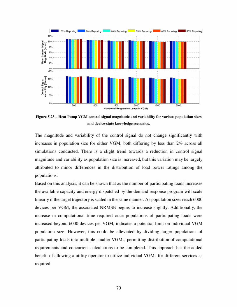
70

Figure 5.23 – Heat Pump VGM control signal magnitude and variability for various population sizes

and device-state knowledge scenarios.

The magnitude and variability of the control signal do not change significantly with

increases in population size for either VGM, both differing by less than 2% across all

simulations conducted. There is a slight trend towards a reduction in control signal

magnitude and variability as population size is increased, but this variation may be largely

attributed to minor differences in the distribution of load power ratings among the

populations.

Based on this analysis, it can be shown that as the number of participating loads increases

the available capacity and energy dispatched by the demand response program will scale

linearly if the target trajectory is scaled in the same manner. As population sizes reach 6000

devices per VGM, the associated NRMSE begins to increase slightly. Additionally, the

increase in computational time required once populations of participating loads were

increased beyond 6000 devices per VGM, indicates a potential limit on individual VGM

population size. However, this could be alleviated by dividing larger populations of

participating loads into multiple smaller VGMs, permitting distribution of computational

requirements and concurrent calculations to be completed. This approach has the added

benefit of allowing a utility operator to utilize individual VGMs for different services as

required.

0%

2%

4%

6%

8%

10%

12%

Mean

Co

ntr

ol

Sig

nal

Mag

nit

ud

e [

%m

ax]

100% Reporting 90% Reporting 80% Reporting 70% Reporting 60% Reporting 50% Reporting

500 1000 1500 3000 4500 60000%

5%

10%

15%

20%

Co

ntr

ol

Sig

nal

Vari

ab

ilit

y [

%m

ax]

Number of Responsive Loads in VGMs

71

Another interesting observation from Figure 5.23 is that under the current target trajectory

the VGMs are generally under-utilized for all but a few minutes of the simulation when the

target reaches the feasible VGM boundary. While this serves to further minimize the

inconvenience on end-user functionality of the participating loads, it is also inefficient for

utility operators. It may be possible to achieve greater utilization with minimal impacts on

end-user functionality by truncating the target trajectory signal to eliminate the large peaks

in demand, effectively allowing the utility operators to request increased amounts of

dispatched energy over the same operational period. This would, however, necessitate the

operation of conventional generation resources, or additional DR programs, to meet the

portion of the target trajectory that was truncated in the first place. Real-world experience

in the operation of DR programs would provide utility operators with further opportunity

to refine DR target determination to optimize the system utilization while ensuring end-use

comfort constraints are not affected. Further, analysis of the system response under

prolonged saturation of the VGMs must be investigated to ensure undesirable behavior is

not inadvertently initiated.

72

6 Conclusions

6.1 Main Contributions

This thesis has examined the effectiveness of aggregate demand response programs

utilizing residential scale loads under varying levels of device-state information. The

development of a new simulation tool to model residential scale loads, as well as a demand

response control framework to test various control algorithms, was created to facilitate the

investigation. The simulation models thermostatically controlled heating loads of

residential homes using an equivalent thermal parameter approach, and electric vehicle

charging loads using a quasi-steady state formulation.

A number of control algorithms were implemented to determine the effectiveness of

demand response programs, culminating in a series of case studies using demand response

to provide ancillary services to power systems operators, and to smooth wind generation

injections into the electrical grid. In addition, the model was adopted to allow the operation

of the demand response program when a portion of the participating loads do not provide

any device-state information to the centralized controller. From these case studies, it was

found that:

• The model works for multiple target trajectories, population sizes and

compositions, over any specified time period. When simulations with reduced

device state-information were evaluated, only small increases in the response error

were noted. Specifically, the NRMSE associated with the demand response

program increases approximately 1% for every 10% decrease in device-state

knowledge in the VGM populations. As a result, even for cases with a device-state

knowledge of 50% of the populations, the associated NRMSE remains below 5%.

This holds true for VGM population sizes ranging from 500 devices to 6000

devices. Further reductions of the NRMSE associated with reduced-knowledge DR

scenarios could be achieved via additional error-correction algorithms integrated

into the DR control algorithms.

• While both investigated loads (Home heat pumps and EV charging) were

successfully implemented as VGMs, the home heat pump loads provided the

73

greatest degree of flexibility in all simulations. This is largely due to the fact that

the heat pump loads are available and participating in the demand response program

throughout the simulation period, while the EV charging loads are regularly

entering and leaving the load community as they are driven by end-users. However,

EV charging loads are not significantly affected by seasonal temperature variations,

whereas the home heat pump loads become less effective as outdoor air

temperatures approach the thermostat set point temperature. For this reason, EV

charging loads exhibit the greatest year-round potential for utilization in demand

response programs.

• The utilization of the demand response resource under the proposed target

trajectories was very low – approximately 15% or less of the potential resource

available over the simulation period. However, this was necessary to ensure that

the highly variable target trajectories remained within the VGM feasible regions

throughout the simulation. It may be possible to better utilize the demand response

resources via optimization of the target trajectory, and optimal dispatch of demand

response resources in conjunction with conventional generation resources.

• Short-duration target trajectories that call upon the full available capacity of the

demand response population do not appear to produce any undesirable behavior

from the system. Some device-level synchronization was observed when the target

trajectory reached the feasible limits of the VGMs, however device-state diversity

rapidly restored without any intervention from the controller when the peak

trajectory was reduced. The effects of long-duration VGM maximum output were

beyond the scope of this thesis.

• The available demand response resource scales proportionally with the population

size of the participating VGMs. Doubling of the participating population of a

particular load type results in a similar doubling of the available capacity and the

energy dispatched by the DR program, provided a similarly scaled target trajectory

is specified. This information will provide a valuable baseline to utility systems

operators when considering how many loads to recruit for a demand response

program.

74

• The error associated with VGMs decreases as the population size is increased to a

certain point, however when the population size reaches 6000 loads per VGM the

associated error begins to increase again. This effect is further amplified in the case

of reduced device-state information scenarios. In addition, with population sizes of

6000 units and larger the associated computational time increases substantially.

The demand response algorithms and the modeling framework developed in this thesis

should be useful in further studies of demand response programs, both at the control

systems level to determine optimal control hardware for participating loads, quantifying

the transient response from a demand response control program, and in large-scale planning

of utility systems operation.

6.2 Recommendations for Future Work

Further development of appropriate algorithms for demand response programs of aggregate

residential scale loads could be carried out in several areas. One key area of improvement

is the implementation of a feedback mechanism to further reduce the error associated with

reduced device-state information scenarios. A simple PID controller could be implemented

to correct for differences between the anticipated response to a given control signal and the

actual response of the system, and applying a gain factor to iteratively tune the controller

for the next time-step.

Another opportunity for future work lies in establishing a rational and economic model to

provide incentives for devices to participate in demand response programs and to quantify

the benefits to the end-user for their participation.

The individual device models used in the simulations provide adequate fidelity for

evaluating the aggregate demand response of the system, but the EV charging model could

be updated to better account for device-level charging phenomenon that are beyond the

scope of the quasi semi-state framework used in this thesis. In addition, inclusion of

vehicle-to-grid functionality would provide insight into the potential of EV charging loads

to provide demand response services beyond what is possible with only deferred charging.

Further, an investigation into the effects of the battery charging trajectory specified by the

demand response program on battery performance and health is necessary prior to

implementation of such a system on actual EVs.

75

As the specified target trajectories in this thesis resulted in low utilization of the demand

response resources, further research into optimal target trajectory formulation would

provide significant value to utility systems operators. This could be completed in

conjunction with work to reduce the computational complexity of the control algorithms

for large population VGMs, as well as large-scale implementations of the simulations to

include multiple VGMs of similar load types. In addition to improving the utilization of

the demand response resource, this would enable to evaluation of much larger DR programs

by recruiting many loads into multiple VGMs, eliminating the associated increased error

and computational requirements of large population VGMs. Furthermore, it is necessary to

investigate the effects of a controller requesting the maximum (or minimum) feasible

output from a VGM for a prolonged period of time. It may be possible to drive the system

to saturation if maximum output is requested for a sufficiently long time, and a recovery

period may be required prior to the VGM being available to provide DR services

immediately following such a request.

Finally, development of consumer-friendly hardware to enable demand response

participation of residential scale loads, and the underlying control structure of such devices

is necessary to bring the simulated demand response programs into the real-world

environment. A discrete control algorithm, similar to the one used by Chassin [20], may be

necessary to fully characterize the control system transfer function and transient response

of the DR system.

76

7 References [1] BC Hydro, “Integrated Resource Plan November 2013,” BC Hydro, Vancouver, BC,

Canada, 2013.

[2] W. Miao, H. Jia, D. Wang, S. Parkinson, C. Crawford, and N. Djilali, “Active Power

Regulation of wind power systems through demand response,” Science China

Technological Series, Vol. 55, No. 6: 1667-1676, June 2012.

[3] S. Parkinson, D. Wang, N. Djilali, “Toward Low Carbon Energy Systems: The

Convergence of Wind Power, Demand Response, and the Electricity Grid.” IEEE

PES Innovative Smart Grid Technologies, 2012.

[4] BC Hydro, “Electric Load Forecast Fiscal 2013 to Fiscal 2033” BC Hydro, Vancouver,

BC, Canada, 2012.

[5] California Independent System Operator, “Demand Response & Proxy Demand

Resource – Frequently Asked Questions 6/24/2011,” CAISO, Folsom, CA, USA,

2011. [Online]. Available:

http://www.caiso.com/Documents/DemandResponseandProxyDemandResourcesFreq

uentlyAskedQuestions.pdf

[6] D. Letto and R. George, “Examination of the Potential for Industrial Loads to Provide

Ancillary Services” ENBALA Power Networks for Oak Ridge National Laboratory

under Subcontract#: 4000114170, November 2012.

[7] Parkinson, Simon, "Managing Sustainable Demand-side Infrastructure for Power

System Ancillary Services", M.A.Sc. Thesis, University of Victoria, December 2011.

[8] J. Matheiu, S. Koch, and D. Callaway, “State Estimation and Control of Electric Loads

to Manage Real-Time Energy Imbalance” IEEE Transactions on power systems, vol

28. No 1. February 2013.

[9] D. Li, Z. Aung, J. Williams, and A. Sanchez, “No peeking: privacy-preserving demand

response system in smart grids,” International Journal of Parallel, Emergent and

Distributed Systems, Vol. 29, No. 3, 290-315, 2014.

77

[10] T. Williams, D. Wang, C. Crawford, and N. Djilali, “Integrating renewable energy

using a smart distribution system: Potential of self-regulating demand response,”

Renewable Energy 52 46-56 (2013).

[11] Canadian Electricity Association, “Power Generation in Canada: A Guide,” Canadian

Electricity Association, Ottawa, ON, Canada, 2006.

[12] G. Cornelis van Kooten. Wind power: the economic impact of intermittency. Letters in

Spatial and Resource Sciences, 3(1):1-17, 1990.

[13] US Energy Information Administration, “Updated Capital Cost Estimates for Utility

Scale Electricity Generating Plants,” US Department of Energy, Washington, DC,

USA 2013 [Online] Available:

http://www.eia.gov/forecasts/capitalcost/pdf/updated_capcost.pdf

[14] E. Yearwood-Lee, “The Site C Dam: Historic Overview and Key Issues,” Legislative

Library of British Columbia, Victoria, BC, Canada, 2007.

[15] J. McLean, “Canada’s Nuclear Energy Sector: Where to from Here?” Canada’s Public

Policy Forum, Ottawa, ON, Canada, January 2014. [Online] Available:

http://site.ebrary.com.ezproxy.library.uvic.ca/lib/uvic/reader.action?docID=10830870

[16] United States Geological Survey, “Hydroelectric power water use,” USGS, US

Department of the Interior, USA, 2014 [Online] Available:

http://water.usgs.gov/edu/wuhy.html

[17] BC Hydro, “Site C Clean Energy Project: Business Case Summary,” BC Hydro,

Vancouver, BC, Canada, 2014.

[18] G. St. Denis and P. Parker, “Community energy planning in Canada: The role of

renewable energy,” Renewable and Sustainable Energy Reviews 13 (2009).

[19] Bonneville Power Authority, “BPA Balancing Reserves Deployed,” BPA, USA, 2015.

[Online] Available:

http://transmission.bpa.gov/business/operations/wind/reserves.aspx

[20] Chassin, David, "New Residential Thermostat for Transactive Systems", M.A.Sc.

Thesis, University of Victoria, December 2014.

78

[21] R.G. Pratt, P.J. Balducci, C. Gerkensmeyer, S. Katipamula, M.C.W. KintnerMeyer,

T.F. Sanquist, K.P. Schneider, and T.J. Secrest. The smart grid: An estimation of the

energy and CO2 benefits. Technical Report 19112 Revision 1, Pacific Northwest

National Laboratory, Richland, Washington, January 2010.

[22] M. Madrigal and K Porter, “Operating and Planning Electricity Grids with Variable

Renewable Generation,” The World Bank, Washington, DC, USA, 2013.

[23] J. Apt and P Jaramillo, “Variable Renewable Energy and the Electricity Grid,” RFF

Press, New York, NY, USA, 2014.

[24] A. Jain and K. Garg, “Variable Renewable Generation and Grid Operation,” 2010

International Conference on Power System Technology, 2010.

[25] S. Sundararagavan and E. Baker. Evaluating energy storage technologies for wind

power integration. Solar Energy 86 (2012).

[26] A. Tuohy, H. Kamath, and L. Rogers, “Evaluation of Storage for Bulk System

Integration of Variable Generation,” 2012 IEEE Power and Energy Society General

Meeting, 2012.

[27] G. Carpinelli, G. Celli, S. Mocci, F. Mottola, F. Pilo, and D. Proto, “Optimal

Integration of Distributed Energy Storage Devices in Smart Grids,” IEEE

Transactions on smart grid, Vol. 4, No, 2, June 2013.

[28] S. Gill, E. Barbour, I. Wilson, and D. Infield, “Maximising revenue for non-firm

distributed wind generation with energy storage in an active management system,”

IET Renewable Power Generation, 2013.

[29] N. O’Connell, P. Pinson, H. Madsen, and M. O’Malley, “Benefits and Challenges of

Electrical Demand Response: A Critical Review. Renewable and Sustainable Energy

Reviews 39 (2014)

[30] P. Faria, Z. Vale, “Demand response in electrical energy supply: An optimal real time

pricing approach,” Energy 36 (2011).

79

[31] D. Chassin, D. Hammerstrom, and J. DeSteese, “The Pacific Northwest Demand

Response Market Demonstration,” 2008 IEEE Power and Energy Society General

Meeting - Conversion and Delivery of Electrical Energy in the 21st Century.

[32] S. Widergren, K. Subbarao, D. Chassin, J. Fuller, and R. Pratt, “Residential Real-time

Price Response Simulation,” 2011 IEEE Power and Energy Society General Meeting.

[33] S. Gyamfi, S. Krumdieck, and T. Urmee, “Residential peak electricity demand response

– Highlights of some behavioural issues,” Renewable and Sustainable Energy

Reviews 25 (2013).

[34] Johanna L. Mathieu. “Modeling, Analysis, and Control of Demand Response

Resources.” PhD dissertation, University of California, Berkley, Spring 2012

[35] D. Wight, et al, “2010 Assessment of Demand Response and Advanced Metering Staff

Report,” Federal Energy Regulatory Commission, USA, 2011.

[36] PJM, “The Evolution of Demand Response in the PJM Wholesale Market,” PJM

Interconnection, October 2014.

[37] D. Hess and J. Coley, “Wireless smart meters and public acceptance: The environment,

limited choices, and precautionary politics,” Public Understanding of Science Vol. 23

No. 6: 688-702. 2014.

[38] Marbek Resource Consultants Ltd. BC Hydro 2007 Conservation Potential Review.

Technical report, Prepared for BC Hydro, 2007.

[39] NRC OEE. 2007 Survey of Household Energy Use: Detailed Statistical Report.

Technical report, Natural Resources Canada Office of Energy Efficiency, 2007.

[40] F.Oldewurtel, et al. “A Framework for and Assessment of Demand Response and

Energy Storage in Power Systems” in 2013 IREP Symposium-Bulk Power System

Dynamics and Control, 2013.

[41] W. Kempton, et al. “A test of vehicle-to-grid (V2G) for energy storage and frequency

regulation in the PJM system.” Technical report, Mid-Atlantic Grid Interactive Cars

Consortium, 2009.

80

[42] C. Quinn, D. Zimmerle, and T.H. Bradley. The effect of communication architecture on

the availability, reliability, and economics of plug-in hybrid electric vehicle-to-grid

ancillary services. J. of Power Sources, 195(5):1500–1509, 2010.

[43] L. Melbourne, “National Travel Survey: England 2013,” Department for Transport,

London, UK, 2013.

[44] R. Mortensen and K. Haggerty. A stochastic computer model for heating and cooling

loads. IEEE Trans. Power Syst., 3(3):854–860, 1990.

[45] D.S. Callaway and I. Hiskens. Achieving controllability of electric loads. Proc. of

IEEE, 99(1):184–199, 2011.

[46] Y. Sun, M. Elizondo, S. Lu, and J. Fuller, “The Impact of Uncertain Physical

Parameters on HVAC Demand Response,” IEEE Transactions on Smart Grid, Vol. 5,

no. 2, March 2014.

[47] D. Wang, S. Parkinson, W. Miao, H. Jia, C. Crawford, and N. Djilali, “Online voltage

security assessment considering comfort-constrained demand response control of

distributed heat pump systems,” Applied Energy 96 (2012).

[48] H. Madsen and J. Holst. Estimation of continuous-time models for the heat dynamics of

a building. Energy and Buildings, 22(1):67–79, 1995.

[49] J. Sager, “Cold Climate Air Source Heat Pumps,” Canmet Energy, National Resources

Canada, 2013. [Online] Available:

http://www.chba.ca/uploads/TRC/May%202013/Cold%20Climate%20Air%20Source

%20Heat%20Pumps%20Presentation%20-%20May%202013.pdf

[50] PNNL. GridLabD - Power System Simulation Software. U.S. Department of Energy:

Pacific Northwest National Laboratory http://www.gridlabd.org/, 2011.

[51] D.S. Callaway. “Tapping the energy storage potential in electric loads to deliver load

following and regulation, with application to wind energy,” Energy Conversion and

Management, 50(9):1389–1400, 2009.

81

[52] John Axsen, et al. “The Canadian Plug-in Electric Vehicle Survey (CPEVS 2013):

Anticipating Purchase, Use, and Grid Interactions in British Columbia.” Simon Fraser

University, Vancouver, BC, Tech. Rep. October, 2013.

[53] J.F. Manwell, J.G. McGowan, and A.L. Rogers. Wind Energy Explained: Theory,

Design and Application, 2nd Edition. John Wiley and Sons, 2010.

[54] C.G. Justus. Winds and Wind System Performance. Franklin Institute Press,

Philadelphia PA, 1978.

[55] J. Cotrell. A preliminary evaluation of a multiple-generator drivetrain configuration for

wind turbines. In Proc. of 21st ASME Wind Energy Symposium, pages 345–352,

2002.

[56] National Renewable Energy Laboratory (Sept 2014). National Wind Technology

Center M2 Tower Data. [Online]. Available: http://www.nrel.gov/midc/nwtc_m2/

[57] Hoevenaars, Eric, "Temporal Resolution in Time Series and Probabilistic Models of

Renewable Power Systems", M.A.Sc. Thesis, University of Victoria, April 2012.

[58] L. Kelly. “Probabilistic modelling of plug-in hybrid electric vehicle: Impacts on

distribution networks in British Columbia.” M.A.Sc. Thesis: University of Victoria

Department of Mechanical Engineering, 2010.

[59] Foley, Aoife M., et al. “Current methods and advances in forecasting of wind power

generation” Renewable Energy 37 (2012)