user guide for ocean data view - national oceanic and ... · user guide for ocean data view (mp) -...
TRANSCRIPT
User Guide for Ocean Data View (mp) - 06.06.2002
User Guide for Ocean Data View Multi-Platform Version
Conditions of Usage
Scientific Use and Teaching
Ocean Data View can be used and distributed free of charge for non-commercial research and teaching purposes. If you use Ocean Data View for your scientific work, you must reference it in your publications as follows:
Schlitzer, R., Ocean Data View, http://www.awi-bremerhaven.de/GEO/ODV, 2002.
Commercial Use
If you plan to use Ocean Data View or any of its components for commercial applications and products, you need to obtain a software license. Please contact the address below for further information.
© 2002 Reiner Schlitzer, Alfred Wegener Institute for Polar and Marine Research, Bremerhaven, Germany
Email: [email protected]
1
User Guide for Ocean Data View (mp) - 06.06.2002
Table of Contents USER GUIDE FOR OCEAN DATA VIEW ....................................................................................................... 1
CONDITIONS OF USAGE ........................................................................................................................................ 1 TABLE OF CONTENTS...................................................................................................................................... 2 1 INTRODUCTION ......................................................................................................................................... 5
1.1 GENERAL OVERVIEW ............................................................................................................................... 5 1.2 EASE OF USE ............................................................................................................................................ 5 1.3 DENSE DATA FORMAT ............................................................................................................................. 5 1.4 EXTENSIBILITY......................................................................................................................................... 5 1.5 DERIVED VARIABLES ............................................................................................................................... 5 1.6 PLOT TYPES.............................................................................................................................................. 6 1.7 GRAPHICS OUTPUT................................................................................................................................... 7 1.8 NETCDF SUPPORT ................................................................................................................................... 7 1.9 ODV MODES ........................................................................................................................................... 7 1.10 INSTALLING OCEAN DATA VIEW.............................................................................................................. 8 1.11 INSTALLING OPTIONAL PACKAGES........................................................................................................... 8
2 ODV SCREEN LAYOUT............................................................................................................................. 9 2.1 MAIN MENU............................................................................................................................................. 9 2.2 3-LINE TEXT WINDOW ............................................................................................................................. 9 2.3 GRAPHICS CANVAS ................................................................................................................................ 10 2.4 STATUS LINE .......................................................................................................................................... 11 2.5 POPUP WINDOWS ................................................................................................................................... 11
3 CREATING COLLECTIONS ................................................................................................................... 13 3.1 COLLECTION FILES SUMMARY ............................................................................................................... 14 3.2 MIGRATING BETWEEN WINDOWS, UNIX AND MACX........................................................................... 14
4 IMPORTING DATA................................................................................................................................... 15 4.1 ODV SPREADSHEET FILES ..................................................................................................................... 15 4.2 WOCE HYDROGRAPHIC DATA .............................................................................................................. 17 4.3 WOD HYDROGRAPHIC DATA ................................................................................................................ 17 4.4 WOA94 HYDROGRAPHIC DATA ............................................................................................................ 17 4.5 SD2 HYDROGRAPHIC DATA................................................................................................................... 18 4.6 OTHER HYDROGRAPHIC DATA ............................................................................................................... 18 4.7 IMPORT OPTIONS DIALOG ...................................................................................................................... 20
5 EXPORTING DATA................................................................................................................................... 22 5.1 SPREADSHEET FILES............................................................................................................................... 22 5.2 ODV COLLECTION................................................................................................................................. 22 5.3 ASCII LISTINGS..................................................................................................................................... 22 5.4 EXPORTING PLOT VALUES ..................................................................................................................... 22
6 DERIVED VARIABLES ............................................................................................................................ 23 6.1 BUILT-IN DERIVED VARIABLES.............................................................................................................. 23 6.2 MACROS OF DERIVED VARIABLES ......................................................................................................... 24 6.3 EXPRESSIONS ......................................................................................................................................... 26
7 USING ODV ................................................................................................................................................ 27 7.1 CHOOSING CURRENT SAMPLE AND CURRENT STATION ......................................................................... 27 7.2 CHANGING VARIABLE SETTINGS............................................................................................................ 27 7.3 CHANGING SELECTION CRITERIA ........................................................................................................... 28 7.4 CHANGING MAP PROJECTIONS ............................................................................................................... 28 7.5 FULL SCREEN STATION MAPS ................................................................................................................ 29
8 PROPERTY-PROPERTY PLOTS............................................................................................................ 30 8.1 ZOOMING AND AUTOMATIC SCALING .................................................................................................... 30 8.2 CHANGING WINDOW LAYOUT................................................................................................................ 30
2
User Guide for Ocean Data View (mp) - 06.06.2002
8.3 CHANGING DISPLAY OPTIONS................................................................................................................ 31 8.4 PRINTING................................................................................................................................................ 33 8.5 POSTSCRIPT FILES.................................................................................................................................. 34 8.6 PNG AND JPG FILES.............................................................................................................................. 34
9 SCATTER PLOTS ...................................................................................................................................... 35 9.1 PRODUCING SCATTER PLOTS.................................................................................................................. 35
10 SECTIONS............................................................................................................................................... 36 10.1 DEFINING A SECTION.............................................................................................................................. 36 10.2 PLOTTING A SECTION ............................................................................................................................. 36 10.3 COLOR-ZOOMING................................................................................................................................... 37 10.4 COLOR MAPPING FUNCTION................................................................................................................... 38 10.5 DISPLAYING GRIDDED FIELDS................................................................................................................ 38 10.6 DIFFERENCE FIELDS ............................................................................................................................... 39
11 ISO-SURFACES...................................................................................................................................... 40 11.1 DEFINING ISO-SURFACES ....................................................................................................................... 40 11.2 PLOTTING SURFACE DISTRIBUTIONS ...................................................................................................... 40
12 NETCDF SUPPORT............................................................................................................................... 42 12.1 NETCDF OVERVIEW.............................................................................................................................. 42 12.2 USING NETCDF FILES ............................................................................................................................ 42
13 MANIPULATING COLLECTIONS..................................................................................................... 46 13.1 CHANGING THE SET OF COLLECTION VARIABLES .................................................................................. 46 13.2 SORTING AND CONDENSING ................................................................................................................... 46 13.3 DELETING SELECTED STATION-SUBSET ................................................................................................. 46
14 UTILITIES............................................................................................................................................... 47 14.1 DATA INVENTORY TABLES..................................................................................................................... 47 14.2 TEMPORAL DATA DISTRIBUTION PLOTS................................................................................................. 47 14.3 DATA RETRIEVAL................................................................................................................................... 47 14.4 GEOSTROPHIC FLOWS ............................................................................................................................ 48 14.5 REFERENCE DATASETS........................................................................................................................... 48 14.6 FINDING OUTLIERS................................................................................................................................. 48 14.7 FINDING REDUNDANT STATIONS............................................................................................................ 49
15 GRAPHICS OBJECTS........................................................................................................................... 50 15.1 ANNOTATIONS........................................................................................................................................ 50 15.2 LINES AND POLYGONS............................................................................................................................ 51 15.3 RECTANGLES AND ELLIPSES................................................................................................................... 51 15.4 SYMBOLS ............................................................................................................................................... 51 15.5 SYMBOL SETS AND LEGENDS ................................................................................................................. 51
16 MORE ….................................................................................................................................................. 53 16.1 GAZETTEER OF UNDERSEA FEATURES.................................................................................................... 53 16.2 DRAG-AND-DROP................................................................................................................................... 53 16.3 ODV COMMAND FILES .......................................................................................................................... 54 16.4 DEFINING PATCHES ................................................................................................................................ 54 16.5 EDITING DATA ....................................................................................................................................... 55 16.6 CHANGING THE COLOR PALETTE ........................................................................................................... 56 16.7 GENERAL SETTINGS ............................................................................................................................... 56 16.8 DIRECTORY STRUCTURE ........................................................................................................................ 57 16.9 HARDWARE REQUIREMENTS .................................................................................................................. 58 16.10 LIMITATIONS ...................................................................................................................................... 58
17 TIPS AND TRICKS ................................................................................................................................ 59 17.1 VISUALIZING DATA FROM XYZ ASCII FILES......................................................................................... 59 17.2 OVERLAYING A PROPERTY DISTRIBUTION WITH CONTOUR-LINES OF ANOTHER PROPERTY ..................... 59 17.3 USING ODV GRAPHICS IN PUBLICATIONS AND ON WEB PAGES............................................................. 60
3

User Guide for Ocean Data View (mp) - 06.06.2002
17.4 PREPARING COASTLINE AND BATHYMETRY FILES ................................................................................. 60
4
User Guide for Ocean Data View (mp) - 06.06.2002
1 Introduction
1.1 General Overview Ocean Data View (ODV) is a computer program for the interactive exploration and graphical display of oceano-graphic and other geo-referenced profile, sequence or gridded data. The multi-platform version of ODV runs on computers with the Windows (9x/NT/2000/XP), Linux, UNIX, and Mac OS X operating systems. ODV data collection and configuration files are platform independent. They can be created on any of the supported sys-tems, and they can be exchanged between the different platforms without translation. ODV lets you interactively browse through large sets of station data. You can produce high-quality station-maps, general property-property plots of one or more stations, scatter plots of selected stations, property sections along arbitrary cruise tracks and property distributions on general iso-surfaces. ODV supports display of original scalar and vector data by col-ored dots, numerical data values or arrows. In addition, two fast gridding algorithms allow color shading and contouring of gridded fields along sections and on iso-surfaces. A large number of derived quantities can be calculated online. These variables can be displayed and analyzed in the same way as the basic variables stored on disk.
1.2 Ease of Use ODV is designed to be flexible and easy-to-use. Users are not required to know the details of the internal data storage format nor are they required to have programming experience. ODV always displays a map of available stations on the screen and facilitates navigating through the data by letting the user select stations, sections and iso-surfaces with the mouse. The screen layout and various other configuration features can be modified easily, and favorite settings can be stored in configuration files on disk for later use. ODV can create and manage very large data collections on relatively inexpensive, widely available and mobile hardware. The data collections can be extended easily when new data arrive. ODV can be useful for scientific data analysis during field programs or back home in the laboratory. It facilitates data quality evaluation and can be helpful for teaching and training.
1.3 Dense Data Format The ODV data format is optimized for variable-length, irregularly-spaced profile, sequence or station data. It provides dense storage and allows instant access to any station, even in very large data collections. The data format is flexible: up to 50 variables can be stored in an individual data collection. Type and number of variables may vary from one collection to another. ODV maintains quality flags associated with every individual data value. These quality flags can be used by ODV as a data quality filter to exclude bad or questionable values from the analysis.
1.4 Extensibility ODV allows easy import of new data into existing collections and also allows easy export of some or all data from a collection. Hydrographic data in the following widely used formats can directly be incorporated into the ODV system:
• WOCE WHP data (distributed via Internet by the WHPO at SCRIPPS), • World Ocean Database (WOD98; WOD01; distributed on CD-ROM by NODC), • World Ocean Atlas 1994 (WOA94; distributed on CD-ROM by NODC), • NODC SD2 data • Java Ocean Atlas spreadsheet format, • ODV spreadsheet format.
1.5 Derived Variables In addition to the basic measured variables stored in the data files, ODV can calculate and display a large num-ber of derived variables. These derived variables are either coded in the ODV software (potential temperature, potential density, dynamic height (all referenced to arbitrary levels), neutral density, Brunt-Väisälä Frequency, sound speed, oxygen saturation, etc.) or are defined in user provided macro files or on-the-fly expressions. The macro language is easy and general enough to allow a large number of applications. Use of expressions and macro files for new derived quantities broadens the scope of ODV considerably and allows easy experimentation with new quantities not yet established in the scientific community. ODV has a built-in macro editor that facili-tates creation and modification of ODV macros.
Any basic or derived variable can be displayed in ODV plots, and they all can be used to define iso-surfaces (e.g., depth horizons, isopycnals, isothermals or isohalines; property minimum or maximum layers like, for in-
5
User Guide for Ocean Data View (mp) - 06.06.2002
stance, the intermediate water salinity minimum layer can be defined as iso-surfaces by use of the zero-crossing of the vertical derivative (a derived quantity) of these variables).
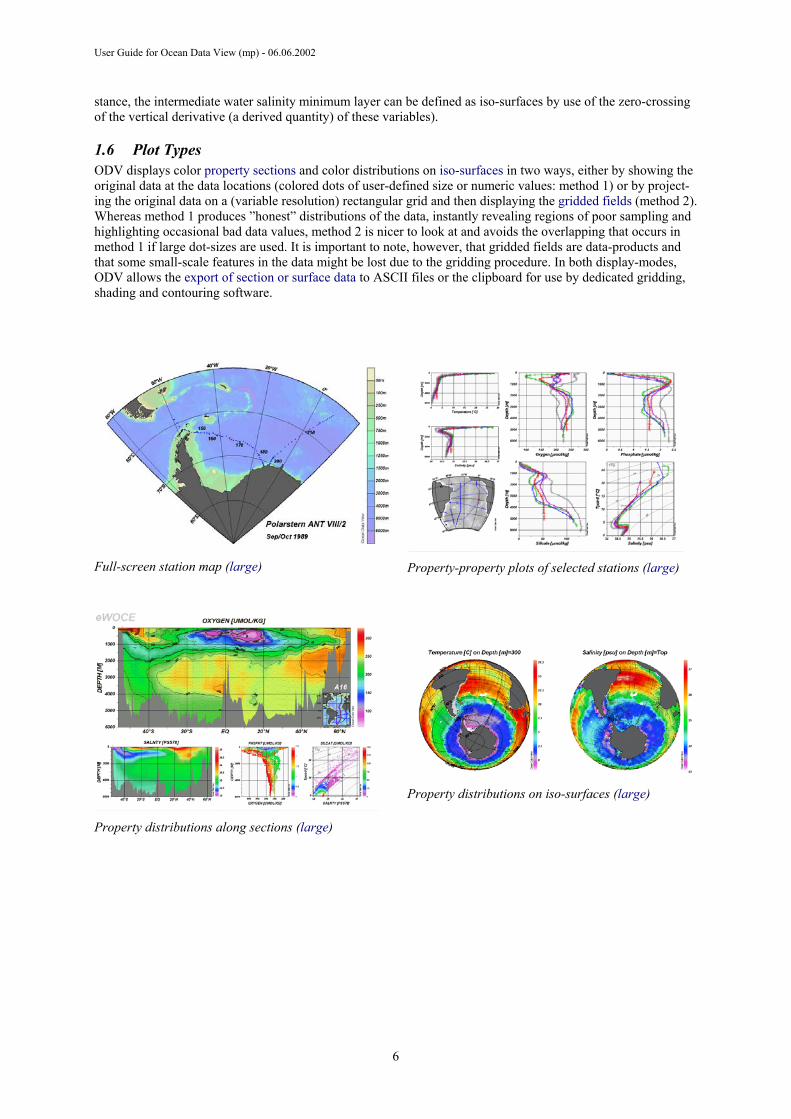
1.6 Plot Types ODV displays color property sections and color distributions on iso-surfaces in two ways, either by showing the original data at the data locations (colored dots of user-defined size or numeric values: method 1) or by project-ing the original data on a (variable resolution) rectangular grid and then displaying the gridded fields (method 2). Whereas method 1 produces ”honest” distributions of the data, instantly revealing regions of poor sampling and highlighting occasional bad data values, method 2 is nicer to look at and avoids the overlapping that occurs in method 1 if large dot-sizes are used. It is important to note, however, that gridded fields are data-products and that some small-scale features in the data might be lost due to the gridding procedure. In both display-modes, ODV allows the export of section or surface data to ASCII files or the clipboard for use by dedicated gridding, shading and contouring software.
Full-screen station map (large)
Property-property plots of selected stations (large)
Property distributions on iso-surfaces (large)
Property distributions along sections (large)
6

User Guide for Ocean Data View (mp) - 06.06.2002
Scatter plots of all stations (large) Arrow Plot
1.7 Graphics Output Color or black and white paper hard copies of the ODV graphics screen (or individual data plots; PostScript, PNG, and JPG only) can be easily obtained via the Print command or by producing PostScript files (.eps). eps files can be printed on any PostScript printer and they can be included in page description documents. ODV can also write the contents of its graphics screen to PNG and JPG files suitable for inclusion in text documents or post-processing with standard graphics software (use PNG as equivalent to GIF). The resolution of ODV PNG and JPG files can be defined by the user and is not tight to the screen resolution.
1.8 NetCDF Support ODV has built-in support for netCDF files, widely used by researchers in different fields of geo-sciences. Using few user specifications and selections, ODV accesses and interprets a given netCDF file in a way that mimics (emulates) a native ODV collection. The full suite of ODV’s analysis and visualization capabilities is provided for the exploration of the data in the netCDF file, and there is no need to translate and re-write the data first. Depending on the structure and contents of a netCDF file, different ODV “emulations” are possible. Settings of individual emulations can be saved on disk for later use. Note that netCDF files are platform independent, and the same file can be used with ODV on all supported platforms.
1.9 ODV Modes ODV can operate in five different modes MAP, STATION, SCATTER, SECTION, and SURFACE. You can easily switch between these modes at any time by pressing keys F8 through F12 or by selecting appropriate options from the background popup menu. The current mode and the active configuration file are always indicated in the right-most pane of the ODV status bar. STATION mode is the default mode (initial mode for new data collec-tions).
MAP mode is intended for full-page station maps and does not provide any data plots. Use this mode to produce high quality cruise maps (define size and position of the map window, choose among five possible map projec-tions, define appropriate coastline and topography settings, mark individual stations with station numbers and cruise labels, produce printouts or PNG, JPG, and EPS PostScript files).
STATION mode (like all following modes) provides a station map and one or more (max. 20) data plot windows. Use this mode to produce X/Y (any basic or derived variable) plots for selected stations. You can select stations by clicking on them in the map with the left mouse button or by specifying cruise and station labels. You add the data of the current station to the plots by pressing p (double clicking on a station selects and plots). Clear the screen and start over by pressing Ctrl-X (this works for all modes).
In SCATTER mode (like for all following modes), data plots support Z variables (any basic or derived variable). The value of a Z variable at a given X/Y point determines the color at X/Y. Plots with Z-variables (for SECTION and SURFACE modes as well) can be displayed in two ways: (1) by placing colored dots or the ac-tual data value at the X/Y locations (default) or (2) as continuous gridded fields estimated on the basis of the observed data. Gridded fields can be color-shaded and/or contoured. Unlike in SECTION and SURFACE modes, data plots in SCATTER mode (with or without Z variable) contain all data points of all stations shown in the map (valid stations).
SECTION mode also supports Z variables on data plots and allows all plot types of the SCATTER mode, but the
7
User Guide for Ocean Data View (mp) - 06.06.2002
set of stations used for the plots is restricted to a section band usually following a given cruise track. Section bands can be defined arbitrarily and their width can be adjusted to select the right set of stations. Use this mode to display property distributions along sections, property/property plots for all stations within a section and to calculate and investigate geostrophic velocities perpendicular to the cross-section.
SURFACE mode lets you define surfaces in 3D (Longitude/Latitude/Depth) space defined as points of constant values of a given variable (e.g., depth, density, temperature, etc) and lets you display property distributions of other variables on this surface. In SURFACE mode you can also produce arbitrary property/property plots for the given surface.
1.10 Installing Ocean Data View There are two ways to install and use Ocean Data View on a supported platform: (1) normal installation or (2) quick installation. Users who anticipate to run ODV regularly should consider a normal installation. This will copy the ODV binaries and support files such as coastline and bathymetry files to the hard disk and ensures optimal execution speed (a minimum of 15MB of disk space is required; more, if you also install optional pack-ages). To perform a normal installation download the latest ODV release files for your platform from http://www.awi-bremerhaven.de/GEO/ODV/downloads-odvmp.html and follow the instructions in the installation readme file.
If you are using ODV only occasionally or if you want to avoid the installation procedure and merely try out ODV, you can run the software from an ODV run-time environment on a CD-ROM or DVD (the eWOCE disk of the WOCE V3 data release provides such a run-time environment). In such a case you start the ODV executa-ble (odvmp.exe on Windows or odvmp for all other platforms) from the binary directory of your platform (Win-dows: bin_w32; Linux: bin_linux-i386, etc.). When you do this for the first time, ODV will prompt you for …
1. the full path-name of the directory that contains the bin_… directory (ODVMPHOME),
2. the full path-name of a directory on your disk for which you have write permission (ODVMPTEMP). This directory will be used by ODV during runtime to write temporary files. You can use the system tmp directory, or you can create a special directory on a local disk (e.g., /odvmptemp) for this purpose. The use of directories on network drives is not recommended because of network transmission delays.
3. the name of your computer,
4. your user or login name.
This completes the quick installation procedure. ODV should run normally, and a re-specification of the quick-installation information should only be required, if you use a different run-time environment.
1.11 Installing Optional Packages To install optional packages like high-resolution coastline and topography files or ready-to-use data collections download the respective package file from http://www.awi-bremerhaven.de/GEO/ODV/downloads-odvmp.html and follow the instructions in the readme files.
8
User Guide for Ocean Data View (mp) - 06.06.2002
2 ODV Screen Layout
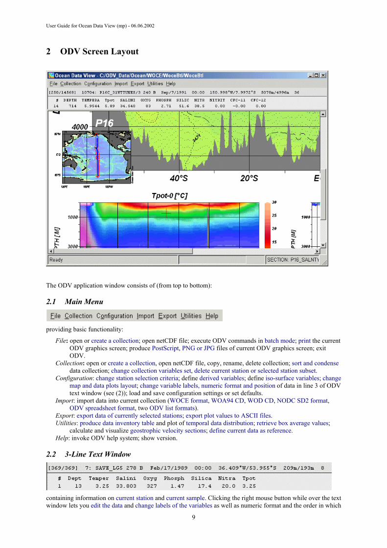
The ODV application window consists of (from top to bottom):
2.1 Main Menu
providing basic functionality:
File: open or create a collection; open netCDF file; execute ODV commands in batch mode; print the current ODV graphics screen; produce PostScript, PNG or JPG files of current ODV graphics screen; exit ODV.
Collection: open or create a collection, open netCDF file, copy, rename, delete collection; sort and condense data collection; change collection variables set, delete current station or selected station subset.
Configuration: change station selection criteria; define derived variables; define iso-surface variables; change map and data plots layout; change variable labels, numeric format and position of data in line 3 of ODV text window (see (2)); load and save configuration settings or set defaults.
Import: import data into current collection (WOCE format, WOA94 CD, WOD CD, NODC SD2 format, ODV spreadsheet format, two ODV list formats).
Export: export data of currently selected stations; export plot values to ASCII files. Utilities: produce data inventory table and plot of temporal data distribution; retrieve box average values;
calculate and visualize geostrophic velocity sections; define current data as reference. Help: invoke ODV help system; show version.
2.2 3-Line Text Window
containing information on current station and current sample. Clicking the right mouse button while over the text window lets you edit the data and change labels of the variables as well as numeric format and the order in which
9

User Guide for Ocean Data View (mp) - 06.06.2002
they are listed in lines 2 and 3. Moving the mouse over a specific variable in the text window gives you more detailed information on this variable in a popup window. You get an overview of current station and sample selection criteria if you move the mouse over the area delimited by [ and ] at the beginning of line 1.
2.3 Graphics Canvas containing the ODV station map and one or more data plots. If only the map is shown, you obtain the data plots by double-clicking on individual stations (STATION mode) or anywhere in the map (all other modes). Clicking the right mouse button (on a Mac hold down the Alt key and click the mouse) while over the map, the data plots or the background area invokes different popup menus:
Background Popup Menu:
clear the screen and restore the station map; print the current ODV graphics screen; produce PostScript, PNG or JPG file of current ODV graphics screen; define derived variables; define iso-surface variables; change map and data plots layout; change variable labels, numeric format and position of data in line 3 of ODV text window; switch between ODV’s MAP, STATION, SCATTER, SECTION and SURFACE modes; exit ODV.
Map Popup Menu:
zoom into map; open map to full domain of collection (de-fined by Define Full Domain); produce standard, global map; change station selection criteria; define section (SECTION mode only); select a new current station by name or internal number; change map display options (map projection, topography and coastline files, station annotation style); define the domain of the current collection.
10
User Guide for Ocean Data View (mp) - 06.06.2002
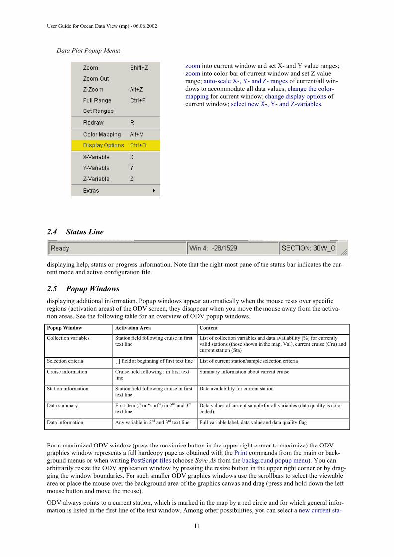
Data Plot Popup Menu:
zoom into current window and set X- and Y value ranges; zoom into color-bar of current window and set Z value range; auto-scale X-, Y- and Z- ranges of current/all win-dows to accommodate all data values; change the color-mapping for current window; change display options of current window; select new X-, Y- and Z-variables.
2.4 Status Line
displaying help, status or progress information. Note that the right-most pane of the status bar indicates the cur-rent mode and active configuration file.
2.5 Popup Windows displaying additional information. Popup windows appear automatically when the mouse rests over specific regions (activation areas) of the ODV screen, they disappear when you move the mouse away from the activa-tion areas. See the following table for an overview of ODV popup windows.
Popup Window Activation Area Content
Collection variables Station field following cruise in first text line
List of collection variables and data availability [%] for currently valid stations (those shown in the map, Val), current cruise (Cru) and current station (Sta)
Selection criteria [ ] field at beginning of first text line List of current station/sample selection criteria
Cruise information Cruise field following : in first text line
Summary information about current cruise
Station information Station field following cruise in first text line
Data availability for current station
Data summary First item (# or “surf”) in 2nd and 3rd text line
Data values of current sample for all variables (data quality is color coded).
Data information Any variable in 2nd and 3rd text line Full variable label, data value and data quality flag
For a maximized ODV window (press the maximize button in the upper right corner to maximize) the ODV graphics window represents a full hardcopy page as obtained with the Print commands from the main or back-ground menus or when writing PostScript files (choose Save As from the background popup menu). You can arbitrarily resize the ODV application window by pressing the resize button in the upper right corner or by drag-ging the window boundaries. For such smaller ODV graphics windows use the scrollbars to select the viewable area or place the mouse over the background area of the graphics canvas and drag (press and hold down the left mouse button and move the mouse).
ODV always points to a current station, which is marked in the map by a red circle and for which general infor-mation is listed in the first line of the text window. Among other possibilities, you can select a new current sta-
11
User Guide for Ocean Data View (mp) - 06.06.2002
tion by clicking on its location in the map with the left mouse button. One of the samples of the current station is the current sample. The data of the current sample are shown in lines 2 and 3 of the text window, and the current sample is marked in the data plots (if present) by a red cross. Among other possibilities, a new current sample (and current station) can be selected by clicking with the left mouse on a data point in any of the data plots.
In order to plot the current station, all stations scatter plots, color sections or iso-surface distributions (in STATION, SCATTER, SECTION, or SURFACE modes, respectively) double-click on the respective station or any point inside the map area, or press p. In STATION mode you can add other stations to the plots by simply double-clicking on other stations. Note that in SECTION mode you have to define a section first for data plots to appear.
12
User Guide for Ocean Data View (mp) - 06.06.2002
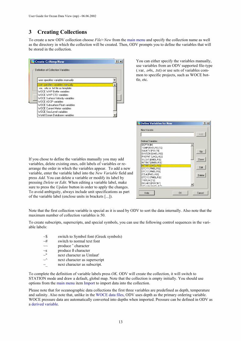
3 Creating Collections To create a new ODV collection choose File>New from the main menu and specify the collection name as well as the directory in which the collection will be created. Then, ODV prompts you to define the variables that will be stored in the collection.
You can either specify the variables manually, use variables from an ODV supported file-type (.var, .o4x, .txt) or use sets of variables com-mon to specific projects, such as WOCE bot-tle, etc.
If you chose to define the variables manually you may add variables, delete existing ones, edit labels of variables or re-arrange the order in which the variables appear. To add a new variable, enter the variable label into the New Variable field and press Add. You can delete a variable or modify its label by pressing Delete or Edit. When editing a variable label, make sure to press the Update button in order to apply the changes. To avoid ambiguity, always include unit specifications as part of the variable label (enclose units in brackets [...]).
Note that the first collection variable is special as it is used by ODV to sort the data internally. Also note that the maximum number of collection variables is 50.
To create subscripts, superscripts, and special symbols, you can use the following control sequences in the vari-able labels:
~$ switch to Symbol font (Greek symbols) ~# switch to normal text font ~~ produce ˜ character ~s produce ß character ~" next character as Umlaut' ~^ next character as superscript ~_ next character as subscript.
To complete the definition of variable labels press OK. ODV will create the collection, it will switch to STATION mode and draw a default, global map. Note that the collection is empty initially. You should use options from the main menu item Import to import data into the collection.
Please note that for oceanographic data collections the first three variables are predefined as depth, temperature and salinity. Also note that, unlike in the WOCE data files, ODV uses depth as the primary ordering variable. WOCE pressure data are automatically converted into depths when imported. Pressure can be defined in ODV as a derived variable.
13
User Guide for Ocean Data View (mp) - 06.06.2002
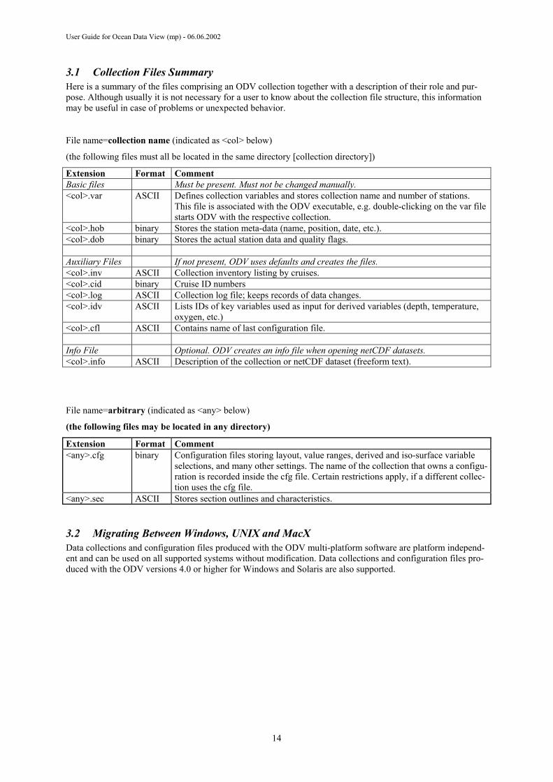
3.1 Collection Files Summary Here is a summary of the files comprising an ODV collection together with a description of their role and pur-pose. Although usually it is not necessary for a user to know about the collection file structure, this information may be useful in case of problems or unexpected behavior.
File name=collection name (indicated as <col> below)
(the following files must all be located in the same directory [collection directory])
Extension Format Comment Basic files Must be present. Must not be changed manually. <col>.var ASCII Defines collection variables and stores collection name and number of stations.
This file is associated with the ODV executable, e.g. double-clicking on the var file starts ODV with the respective collection.
<col>.hob binary Stores the station meta-data (name, position, date, etc.). <col>.dob binary Stores the actual station data and quality flags. Auxiliary Files If not present, ODV uses defaults and creates the files. <col>.inv ASCII Collection inventory listing by cruises. <col>.cid binary Cruise ID numbers <col>.log ASCII Collection log file; keeps records of data changes. <col>.idv ASCII Lists IDs of key variables used as input for derived variables (depth, temperature,
oxygen, etc.) <col>.cfl ASCII Contains name of last configuration file. Info File Optional. ODV creates an info file when opening netCDF datasets. <col>.info ASCII Description of the collection or netCDF dataset (freeform text).
File name=arbitrary (indicated as <any> below)
(the following files may be located in any directory)
Extension Format Comment <any>.cfg binary Configuration files storing layout, value ranges, derived and iso-surface variable
selections, and many other settings. The name of the collection that owns a configu-ration is recorded inside the cfg file. Certain restrictions apply, if a different collec-tion uses the cfg file.
<any>.sec ASCII Stores section outlines and characteristics.
3.2 Migrating Between Windows, UNIX and MacX Data collections and configuration files produced with the ODV multi-platform software are platform independ-ent and can be used on all supported systems without modification. Data collections and configuration files pro-duced with the ODV versions 4.0 or higher for Windows and Solaris are also supported.
14

User Guide for Ocean Data View (mp) - 06.06.2002
4 Importing Data
4.1 ODV Spreadsheet Files ODV can read and import data from a variety of spreadsheet-type ASCII files. The data from these files can be imported into existing data collections or can be used to create new collections. ODV supports files with or without station metadata information and with or without column label information. You may use either TAB or ; or SPACE or / as column separation characters, and the missing value indicator may be any dedicated number or a blank field. A detailed list of specifications for the general ODV spreadsheet format is given in the table below.
Note that ODV spreadsheet files may contain data for many stations from many cruises. All observed levels of a given station must be in consecutive order but need not necessarily be sorted. Whenever either one of the entries Cruise, Station, Type, mon/day/yr, hh:mm, Lon (°E) or Lat (°N) changes from one line to the next, ODV inter-prets this as the beginning of a new station.
The procedure for importing general ODV spreadsheet files is described in the following. Note that for the more restricted generic ODV spreadsheet format described below, the import procedure is usually much simpler and requires almost no user interaction.
To import data from a general ODV spreadsheet file into the currently open collection choose Im-port>SpreadSheet and use the standard file-select dialog to identify the data file that you want to import. If the file format deviates from the generic ODV spreadsheet format (see below), a Spreadsheet File Properties dialog box appears that lets you choose the column separation character and the missing data value (fields that contain this value or are empty are considered missing). You can also identify the line that contains the column labels (leave empty if not present) and the first data line. ODV provides reasonable defaults for all items and only a few changes are necessary in most cases. For the Column Sep. Character choose the character that will give a verti-cal list of labels in the Column Labels box. Press OK when all spreadsheet file properties are set or Cancel to abort the import.
If the labels for the metadata columns deviate from the specifications of the generic ODV spreadsheet format (see below), a Header Variable Association dialog box appears that lets you associate input columns with the collection metadata variables, or it lets you set defaults for those variables not provided in the input file. Already associated variables are marked by asterisks (*). To define a new association select items in the Source File and Target Collection lists and press Associate. To invoke a conversion during import press Convert and choose one of the available conversion algorithms. To delete an existing association, select the respective variables and press Undo. If the import file does not contain information for one or more collection header variables you can specify defaults: (1) select the respective target variable; (2) press Set Default and (3) enter the default value. Note that the specified default settings are used for all data lines in the file. Press OK when done or Cancel to abort the import procedure. Finally specify import options and press OK to start the data import.
Note that files that deviate from the generic ODV spreadsheet format (see below) should not be dragged and dropped onto the ODV desktop icon or an open ODV window.
4.1.1 General Format
General ASCII coding
File extension any
Columns
Station metadata information and data values for up to 50 variables are stored in sepa-rate columns. Some or all metadata columns may be missing. Metadata and data col-umns can be in arbitrary order. The line containing the column labels (if present, see below) and all data lines in the file must have the same number of columns.
Column separation character
TAB or ; or SPACE or /
IMPORTANT: Note that cruise and station labels must not contain the column separa-tion character; e.g., using SPACE or / as column separation character will break the label “CFC [um/kg]” into two tokens.
Column labels line
1. May be missing; if provided must appear before any data line.
2. Labels for metadata and data columns are arbitrary. Recommended header labels are: "Cruise", "Station", "Type", "mon/day/yr", "hh:mm", "Lon (°E)", "Lat (°N)", "Bot. Depth [m]".
3. Labels for data variables can be up to 60 characters long and should include unit specifications enclosed in brackets [ ].
4. Each column for a data variable can have an optional quality-flag column immedi-
15
User Guide for Ocean Data View (mp) - 06.06.2002
ately following the variable to which it belongs. The label of a quality-flag column must be either QF or QF:* where * represents an arbitrary character sequence.
Data lines
1. May start at any line of the file. All lines following the first data line are assumed to be data lines as well (no comments at the end of the file!).
2. Each line contains metadata and data for one observed level. All observed levels of a given station must be in consecutive order but need not be sorted. An ODV Spreadsheet file can store the data of many stations from many cruises.
3. Station “Type” is a single character string (use B for stations with less than about 250 levels (e.g., bottle data) and C for stations with more than about 250 levels (e.g., CTD, XBT, etc.). Specifying * for “Type” lets ODV make the choice.
4. If “Bot. Depth” is not available, use “0” (zero) in this field.
5. The station header information (if header columns are included) must be present on all lines.
Quality flag columns
1. If data quality information is available for a given variable, this information is stored in the column immediately following to the right of the variable to which it belongs.
2. Quality flags are single digit integers: 0=good, 1=unknown, 4=questionable, 8=bad.
Missing data value blank field or any numerical value beyond the range of good data.
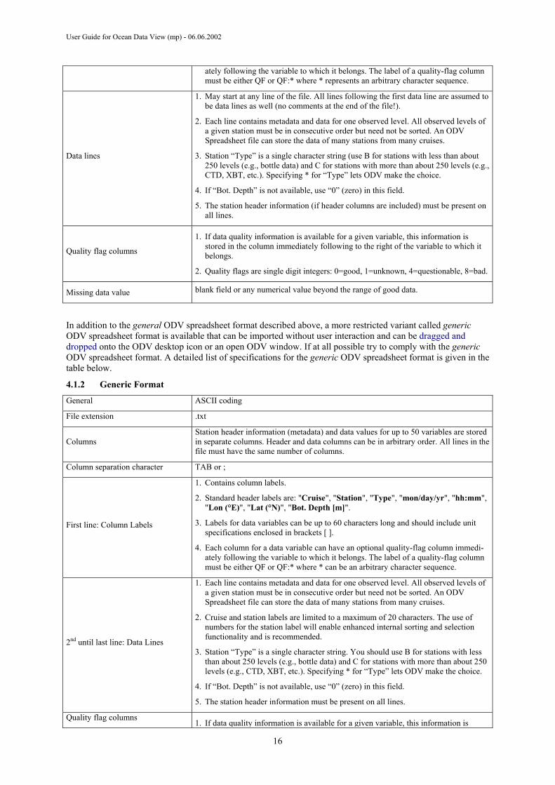
In addition to the general ODV spreadsheet format described above, a more restricted variant called generic ODV spreadsheet format is available that can be imported without user interaction and can be dragged and dropped onto the ODV desktop icon or an open ODV window. If at all possible try to comply with the generic ODV spreadsheet format. A detailed list of specifications for the generic ODV spreadsheet format is given in the table below.
4.1.2 Generic Format
General ASCII coding
File extension .txt
Columns Station header information (metadata) and data values for up to 50 variables are stored in separate columns. Header and data columns can be in arbitrary order. All lines in the file must have the same number of columns.
Column separation character TAB or ;
First line: Column Labels
1. Contains column labels.
2. Standard header labels are: "Cruise", "Station", "Type", "mon/day/yr", "hh:mm", "Lon (°E)", "Lat (°N)", "Bot. Depth [m]".
3. Labels for data variables can be up to 60 characters long and should include unit specifications enclosed in brackets [ ].
4. Each column for a data variable can have an optional quality-flag column immedi-ately following the variable to which it belongs. The label of a quality-flag column must be either QF or QF:* where * can be an arbitrary character sequence.
2nd until last line: Data Lines
1. Each line contains metadata and data for one observed level. All observed levels of a given station must be in consecutive order but need not be sorted. An ODV Spreadsheet file can store the data of many stations from many cruises.
2. Cruise and station labels are limited to a maximum of 20 characters. The use of numbers for the station label will enable enhanced internal sorting and selection functionality and is recommended.
3. Station “Type” is a single character string. You should use B for stations with less than about 250 levels (e.g., bottle data) and C for stations with more than about 250 levels (e.g., CTD, XBT, etc.). Specifying * for “Type” lets ODV make the choice.
4. If “Bot. Depth” is not available, use “0” (zero) in this field.
5. The station header information must be present on all lines.
Quality flag columns 1. If data quality information is available for a given variable, this information is
16
User Guide for Ocean Data View (mp) - 06.06.2002
stored in the column immediately following to the right of the variable to which it belongs.
2. Quality flags are single digit integers: 0=good, 1=unknown, 4=questionable, 8=bad.
Missing data value blank field or –1.e10.
Import files in generic ODV Spreadsheet Format can be processed by ODV in a semi-automatic way: the identi-fication of header columns requires no user interaction and these files can be dragged-and-dropped onto the ODV icon or an open ODV window.
To import data from a generic ODV spreadsheet file into the currently open collection choose Im-port>SpreadSheet and use the standard Windows file-select dialog to identify the data file that you want to im-port. Specify import options and press OK to start the data import.
4.2 WOCE Hydrographic Data You can import WOCE hydrographic data (in WHP exchange format) into the currently open ODV collection. First, download the data files from the WHP DAC (http://whpo.ucsd.edu/) into an empty directory on your disk (source directory). To import bottle data, choose Import>WOCE WHP Bottle (exchange format)>Single File from ODV’s main menu. Use the standard file-select dialog to select the WHP data set on your disk (note that the default extension of WHP exchange files is .csv; if your exchange file has a different extension, choose file-type “All Files” on the file-select dialog). Then specify import options and press OK to start the data import. ODV will read and import all stations in the WOCE data file. Note that ODV identifies and imports the WOCE data quality flags in addition to the actual data values. These quality flags can later be used to filter the data by excluding, for instance, bad or questionable data from the analysis. (You can modify the data quality filter by choosing selection criteria from the map popup menu (choose the Sample Selection tab).)
To import CTD data, choose Import>WOCE WHP CTD (exchange format)>Single File from ODV’s main menu and select the .zip file that contains the CTD data to be imported. If required, you may then specify sub-sampling parameters (default is no sub-sampling). Then, ODV will unpack the .zip file and imports all CTD stations into the currently open collection. ODV can handle up to 20,000 observed levels per station. If a station contains more levels, it will be truncated.
Note that ODV automatically converts the pressure data in the source files to depth in the collection. If you need pressure as a variable, activate the derived variable Pressure(Depth).
4.3 WOD Hydrographic Data You can use ODV to import original hydrographic data directly from the distribution CDs or from on-line files of the World Ocean Database by choosing Import>World Ocean Database>Single File. Use the standard Win-dows file-select dialog to identify a zipped data file (*.gz) of the WOD data set that you want to import (choose file-type “All Files (*.*)” if you want to select a WOD file that is already unzipped). Specify station selection criteria to be satisfied by WOD stations or simply press OK to import all stations falling into the current map domain, specify import options and press OK to start the data import. ODV will read the selected WOD data file and import all stations that satisfy the station selection criteria. The cruise label of imported stations consists of the WOD identifier, e.g., ”WOD98”, “WOD01”, etc. followed by the two digit NODC country-code and the six digit OCL cruise number. The unique OCL profile number is used by ODV as station number. ODV recognizes and uses data quality flags found in the import files.
You can import data from multiple WOD files in a single import operation using the same station selection crite-ria and import options. To do so, you have to prepare a ASCII file (default extension .lst) that contains the names of the files to be imported (full pathnames, one name per line). Choose Import>World Ocean Data-base>Multiple Files, specify station selection criteria to be satisfied by WOD stations (simply press OK to im-port all stations falling into the current map domain), specify import options and press OK to start the data im-port. ODV will read all the files listed in the ASCII file and will import all stations that satisfy the station selec-tion criteria.
Note that only stations falling into the current map domain are imported into the collection. To make sure that all stations are imported, choose Global Map from the map popup menu before starting the import.
4.4 WOA94 Hydrographic Data You can use ODV to import original hydrographic data directly from the distribution CDs of the World Ocean Atlas 1994 by choosing Import>World Ocean Atlas 94>Single File. Use the standard Windows file-select dialog
17

User Guide for Ocean Data View (mp) - 06.06.2002
to identify the data file (*.ol) of the WOA94 data set that you want to import. Specify station selection criteria to be satisfied by WOA94 stations (simply press OK to import all stations falling into the current map domain), specify import options and press OK to start the data import. ODV will read the selected WOA94 data file and import all stations that satisfy the station selection criteria.
You can import data from multiple WOA94 files using the same station selection criteria and import options in a single import operation. To do so, prepare an ASCII file (default extension .lst) containing the names of the files to be imported (full pathnames, one per line). Choose Import>World Ocean Atlas 94>Multiple Files, specify station selection criteria to be satisfied by WOA94 stations (simply press OK to import all stations falling into the current map domain), specify import options and press OK to start the data import. ODV will read all the files listed in the ASCII file and will import all stations that satisfy the station selection criteria.
Note that only stations falling into the current map domain are imported into the collection. To make sure that all stations are imported, choose Global Map from the map pop-up menu before starting the import.
4.5 SD2 Hydrographic Data You can use ODV to import original hydrographic data from NODC SD2 files by choosing Import>NODC SD2 Format>Single File. Use the standard Windows file-select dialog to identify the data file that you want to im-port. Specify import options and press OK to start the data import.
If you want to import multiple SD2 files, put all the SD2 files in a single directory and produce a file containing the list of SD2 file-names that you want to import (default list-file extension .lst; one file-name per line). Choose Import>NODC SD2 Format>Multiple Files and select the list-file.
4.6 Other Hydrographic Data If your hydrographic data are not in WOCE WHP, WOA94 or NODC SD2 format you can import these data into ODV collections using the ODV spreadsheet format described above. For backward compatibility ODV still supports the ODV4.x ASCII format that permits long cruise and station labels as well as data quality flag values for every actual data value. Users of old ODV versions may translate data via the ODV3.0 ASCII exchange format.
4.6.1 .o4x Exchange Format
The .o4x ASCII exchange format is a single-file format. Information on variables as well as the data values and quality flags for all stations to be imported are contained in one file (default extension .o4x). This file must con-tain information on type of data as well as number and labels of variables at the top (see below or file im-port4.o4x in the ODV samples directory). (Note that in the example below, the "....+." lines at the top and bottom only serve as rulers and are not part of the file.)
Sample .o4x variables section ....+....1....+....2....+....3....+....4....+....5....+....6....ODV4.0 ListingFile Name: import4.o4x
Type: HYDNstat: 12
Variables: 8
Depth [m] 6.0Temperature [°C] 8.2Salinity [psu] 8.3Oxygen [~$m~#mol/kg] 6.0Phosphate [~$m~#mol/kg] 8.2Silicate [~$m~#mol/kg] 8.1Nitrate [~$m~#mol/kg] 7.1Nitrite [~$m~#mol/kg] 6.1....+....1....+....2....+....3....+....4....+....5....+....6....
One empty line separates the variables section of the data file from the header line of the first station (see file import4.o4x in the ODV samples directory for an example). Station header lines must start with a # in column 1. The following items are: (1) cruise-label of the station (cols. [3:22], format a20); (2) station-label ([24:43], a20); (3) station-type (either B, C or X for bottle, CTD or XBT data; [45:45], a1); (4) date mm/dd/yyyy ([47:66], i2,1x,i2,1x,i4); (5) east longitude (decimal; [58:64], f7.3); (6) north latitude (decimal; [66:72], f7.3); (7) bottom depth ([m]; [74:78], i5); (8) depth of deepest observation ([m]; [80:84], i5); (9) number of depths sampled ([85:89], i5); (10) number of variables for which data are provided in the file ([91:93], i3). In the example file, the station 06MT18/558 is of type "Bottle", it contains 14 observed depths and data for 8 variables at these ob-served depths are to follow. These variables have to be identified by specifying their numbers (as defined in the
18
User Guide for Ocean Data View (mp) - 06.06.2002
variables section at the beginning of the file) on the second header line (e.g., 1 represents Depth and, for in-stance, 6 represents Silicate). Note that as the only format restriction, the variable numbers on the second header line have to be separated by at least one blank.
For each observed depth (14 in the example file) one line of data has to follow. Each of these lines must contain a data and quality flag value for every variable specified on the second header line in that order. Missing values have to be set to -1.000E+10 in the data file. Note that data and quality flag values have to be separated by at least one space. Quality flags are single digit integers with the following meaning: 0=Good, 1=Unknown, 4=Questionable, 8=Bad. Immediately after the last data line of a given station follows the first header line (start-ing with the #) of the next station to be imported or the end-of-file if the station is the last to be read.
Once the.o4x file has been created, run ODV and open or create the collection that is to receive the new data. Then choose ODV4.x Listing from the Import menu. Select the ASCII data file created above as data import file. Specify import options and press OK to start the data import. ODV will then read the import file and add/merge the stations to the collection. Note that you can also drag-and-drop .o4x files onto ODV.
4.6.2 .o3x Exchange Format
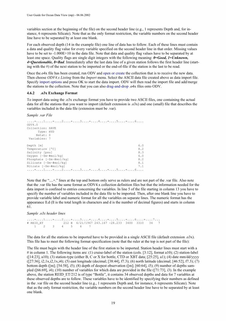
To import data using the .o3x exchange format you have to provide two ASCII files, one containing the actual data for all the stations that you want to import (default extension is .o3x) and one (small) file that describes the variables included in the data file (extension must be .var).
Sample .var File ....+....1....+....2....+....3....+....4....+....5....+....6....ODV4.0Collection: SAVE
Type: HYDNstat: 0
Variables: 7
Depth [m] 6.0Temperature [°C] 8.2Salinity [psu] 8.3Oxygen [~$m~#mol/kg] 6.0Phosphate [~$m~#mol/kg] 8.2Silicate [~$m~#mol/kg] 8.1Nitrate [~$m~#mol/kg] 7.1....+....1....+....2....+....3....+....4....+....5....+....6....
Note that the “....+.” lines at the top and bottom only serve as rulers and are not part of the .var file. Also note that the .var file has the same format as ODV4.x collection definition files but that the information needed for the data import is confined to entries concerning the variables. In line 5 of the file starting in column 13 you have to specify the number of variables included in the data file to be imported. Then, after one blank line you have to provide variable label and numeric format for all the variables on separate lines. The numeric format has the appearance ll.d (ll is the total length in characters and d is the number of decimal figures) and starts in column 61.
Sample .o3x header lines ....+....1....+....2....+....3....+....4....+....5....+....6....+....7...# REID_ET 212 B 6/21/1967 243.167 -28.233 3400 3310 34 7
1 2 3 4 5 6 7
The data for all the stations to be imported have to be provided in a single ASCII file (default extension .o3x). This file has to meet the following format specification (note that the ruler at the top is not part of the file):
The file must begin with the header line of the first station to be imported. Station header lines must start with a # in column 1. The following items are: (1) cruise-label of the station (cols. [3:12], format a10); (2) station-label ([14:23], a10); (3) station-type (either B, C or X for bottle, CTD or XBT data; [25:25], a1); (4) date mm/dd/yyyy ([27:36], i2,1x,i2,1x,i4); (5) east longitude (decimal; [38:44], f7.3); (6) north latitude (decimal; [46:52], f7.3); (7) bottom depth ([m]; [54:58], i5); (8) depth of deepest observation ([m]; [60:64], i5); (9) number of depths sam-pled ([66:69], i4); (10) number of variables for which data are provided in the file ([71:73], i3). In the example above, the station REID_ET/212 is of type “Bottle”, it contains 34 observed depths and data for 7 variables at these observed depths are to follow. These variables have to be identified by specifying their numbers as defined in the .var file on the second header line (e.g., 1 represents Depth and, for instance, 6 represents Silicate). Note that as the only format restriction, the variable numbers on the second header line have to be separated by at least one blank.
19
User Guide for Ocean Data View (mp) - 06.06.2002
For each observed depth (34 in the example above) one line of data has to follow. Each of these lines must con-tain a numerical value for every variable specified on the second header line in that order. Missing values have to be set to -1.000E+10 in the data file. Immediately after the last data line of a given station follows the first header line (starting with the #) of the next station to be imported or the end-of-file if the station is the last to be read.
Once the .var and .o3x files have been created, run ODV and open or create the collection that is to receive the new data. Then choose ODV3.0 Listing from the Import menu. Select the ASCII data file created above as data import file and identify the variables to be imported by selecting the import .var file as the data source. Specify import options and press OK to start the data import. ODV will then read the import file and add/merge the sta-tions to the collection. Note that the data quality flags are set to Unknown if you import data using ODV3.0 exchange format.
4.7 Import Options Dialog
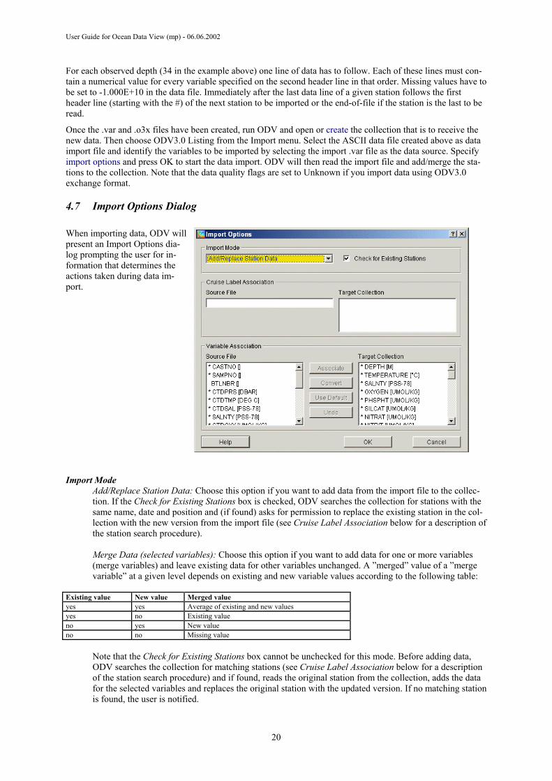
When importing data, ODV will present an Import Options dia-log prompting the user for in-formation that determines the actions taken during data im-port.
Import Mode Add/Replace Station Data: Choose this option if you want to add data from the import file to the collec-tion. If the Check for Existing Stations box is checked, ODV searches the collection for stations with the same name, date and position and (if found) asks for permission to replace the existing station in the col-lection with the new version from the import file (see Cruise Label Association below for a description of the station search procedure).
Merge Data (selected variables): Choose this option if you want to add data for one or more variables (merge variables) and leave existing data for other variables unchanged. A ”merged” value of a ”merge variable” at a given level depends on existing and new variable values according to the following table:
Existing value New value Merged value yes yes Average of existing and new values yes no Existing value no yes New value no no Missing value
Note that the Check for Existing Stations box cannot be unchecked for this mode. Before adding data, ODV searches the collection for matching stations (see Cruise Label Association below for a description of the station search procedure) and if found, reads the original station from the collection, adds the data for the selected variables and replaces the original station with the updated version. If no matching station is found, the user is notified.
20
User Guide for Ocean Data View (mp) - 06.06.2002
Update Data (selected variables): Choose this option if you want to update data for one or more variables (update variables) and leave existing data for other variables unchanged. An ”updated” value of an ”up-date variable” at a given level only depends on the new variable values and existing values are discarded. Note that the Check for Existing Stations box cannot be unchecked for this mode. Before updating data, ODV searches the collection for matching stations (see Cruise Label Association below for a description of the station search procedure) and if found, reads the original station from the collection, updates the data for the selected variables and replaces the original station with the updated version. If no matching station is found, the user is notified.
Cruise Label Association When replacing or merging data, ODV first has to search the target collection for an existing station that matches the given station to be imported. This search is made by comparing cruise name, station name, station type, lon/lat position and date. For a successful match, all items except cruise name are required to be identical. For cruise name you can establish alias names using the Target and Source combo-boxes. If, for instance, in the existing collection a set of stations is named 06MT15/3 and in the import file the same stations are named METEOR15/3 you can set up an alias name by first choosing 06MT15/3 from the Target combo-box and then typing METEOR15/3 in the source field. Note that the default entries in the Source field are the same as the target names, so in case the cruise labels in the import file and in the collection are identical, you do not need to modify the Cruise Label Association at all.
Variable Association Usually the number, order and meaning of variables stored in the import file differ from the number, or-der and meaning of variables stored in the collection. Therefore you must establish a source/target asso-ciation of variables. ODV automatically associates variables with matching labels (name and units). Note that associated variables are marked with a *. You can click on such a variable to identify its associated variable. To establish a variable association manually click on the respective source variable, then click on the tar-get variable to be associated with the source variable and either press the Associate or Convert buttons. Use Associate if the data values in the import file should be imported without modification, but use Con-vert if you need to transform units during import. When using Convert, you can choose between prede-fined, commonly used transformations and you can establish your own general linear transformation for-mula. For ODV Spreadsheet imports you can set default values for target variables for which no corresponding source variable is provided in the import file. This is useful, for instance, if you import longitude/latitude maps of some quantity Z from ASCII files containing three columns X/Y/Z, but not containing data for the specific surface or depth level. To set a default value for a target value, first select a the variable in the Target Collection list, then press the Use Default button and enter the desired default value for this target variable. Note that this target variables is now marked with a + sign. The specified value will be used for every observed level of every station imported during this operation. Source variables not associated with a target variable will not be imported into the collection. If you merge data into the collection, establish associations only for those variables that you want to add to the collection. Note that the first variable in any ODV collection must be associated in any case.
21

User Guide for Ocean Data View (mp) - 06.06.2002
5 Exporting Data
5.1 Spreadsheet Files You can export the data of the currently selected stations into a single ASCII spreadsheet file by choosing Ex-port>ODV SpreadSheet from ODV's main menu. Then select the variables to be included in the export file (de-fault: all variables) and specify destination directory and file-name using the standard file-select dialog-box. Note that spreadsheet files can be re-imported using the Import>ODV SpreadSheet. Note that valid ODV spread-sheet names may not contain spaces or any of the following characters: \ / :.
5.2 ODV Collection You can export the data of the currently selected stations into a new ODV collection by choosing Export>ODV Collection from ODV's main menu. Then select the variables to be included in the new collection (default: all variables) and specify destination directory and file-name using the standard file-select dialog-box. Note that valid ODV collection names may not contain spaces or any of the following characters: \ / :.
5.3 ASCII Listings You can export the data of the currently selected stations into a single ASCII listing file by choosing Ex-port>ODV4.x Listing from ODV's main menu. Then select the variables to be included in the export file (de-fault: all variables) and specify destination directory and file-name using the standard Windows file-select dia-log-box. Note that ODV4.x Listing files can be re-imported using the Import> ODV4.x Listing. For further in-formation on the ODV4.x Listing format click here. Note that valid ODV listing names may not contain spaces or any of the following characters: \ / :.
5.4 Exporting Plot Values You can export the data values displayed in ODV plot windows to ASCII files for subsequent processing (aver-aging, gridding, contouring, etc.) by choosing Export>Export Plot Values from ODV’s main menu. Enter a de-scriptive text identifying the data of this export (txtID) and click OK. ODV will create a sub-directory in the local ODV directory (normally <home>\odv_local) named export\txtID. All exported files will be written to this directory. If it already exists, ODV asks for your permission to delete all files from the directory before continu-ing. Note that the names of the exported files start with “win?” where ? represents the respective window num-ber. The actual x-y-z-sigma_z data are found in files win?.oai (one data point per line).
For windows with gridded fields, ODV also exports the results of the gridding operation (files win?.oao). The format of the .oao files is as follows:
0 (ignore)
nx ny (no of x and y grid-points)
... nx X-grid values ... (X-grid positions)
... ny Y-grid values ... (Y-grid positions)
... nx*ny gridded values ... (estimated field, X-line by X-line starting at first Y-grid value)
22
User Guide for Ocean Data View (mp) - 06.06.2002
6 Derived Variables In addition to the basic variables stored in the collection files, ODV can calculate a large number of derived variables which (once defined) are available for analysis and use in the data plots in the same way as the basic variables. There are three types of derived variables:
• built-in derived variables including many commonly used parameters from physical and chemical oceanography.
• macro files of user defined expressions stored in files for use with arbitrary ODV collections.
• expressions defined by the user “on-the-fly” for the current collection only.
To define or delete derived variables choose the Derived Variables option from the background popup menu or Configuration>Derived Variables from the main menu. To add a macro choose Macro File from the “Choices” list; to add an user defined expression choose Expression. To add a built-in derived variable choose any other item in the “Choices” list.
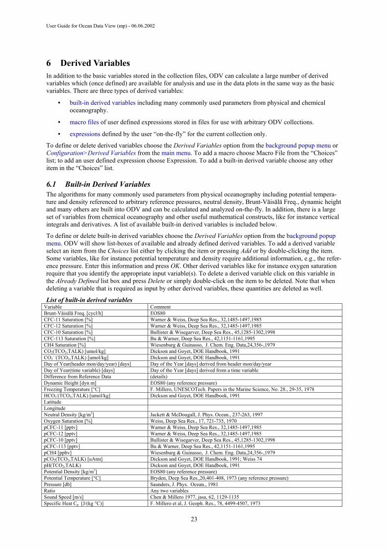
6.1 Built-in Derived Variables The algorithms for many commonly used parameters from physical oceanography including potential tempera-ture and density referenced to arbitrary reference pressures, neutral density, Brunt-Väisälä Freq., dynamic height and many others are built into ODV and can be calculated and analyzed on-the-fly. In addition, there is a large set of variables from chemical oceanography and other useful mathematical constructs, like for instance vertical integrals and derivatives. A list of available built-in derived variables is included below.
To define or delete built-in derived variables choose the Derived Variables option from the background popup menu. ODV will show list-boxes of available and already defined derived variables. To add a derived variable select an item from the Choices list either by clicking the item or pressing Add or by double-clicking the item. Some variables, like for instance potential temperature and density require additional information, e.g., the refer-ence pressure. Enter this information and press OK. Other derived variables like for instance oxygen saturation require that you identify the appropriate input variable(s). To delete a derived variable click on this variable in the Already Defined list box and press Delete or simply double-click on the item to be deleted. Note that when deleting a variable that is required as input by other derived variables, these quantities are deleted as well.
List of built-in derived variables Variable Comment Brunt-Väisälä Freq. [cycl/h] EOS80 CFC-11 Saturation [%] Warner & Weiss, Deep Sea Res., 32,1485-1497,1985 CFC-12 Saturation [%] Warner & Weiss, Deep Sea Res., 32,1485-1497,1985 CFC-10 Saturation [%] Bullister & Wisegarver, Deep Sea Res., 45,1285-1302,1998 CFC-113 Saturation [%] Bu & Warner, Deep Sea Res., 42,1151-1161,1995 CH4 Saturation [%] Wiesenburg & Guinasso, J. Chem. Eng. Data,24,356-,1979 CO2(TCO2,TALK) [umol/kg] Dickson and Goyet, DOE Handbook, 1991 CO3
- -(TCO2,TALK) [umol/kg] Dickson and Goyet, DOE Handbook, 1991 Day of Year(header mon/day/year) [days] Day of the Year [days] derived from header mon/day/year Day of Year(time variable) [days] Day of the Year [days] derived from a time variable Difference from Reference Data (details) Dynamic Height [dyn m] EOS80 (any reference pressure) Freezing Temperature [°C] F. Millero, UNESCOTech. Papers in the Marine Science, No. 28., 29-35, 1978 HCO3
-(TCO2,TALK) [umol/kg] Dickson and Goyet, DOE Handbook, 1991 Latitude Longitude Neutral Density [kg/m3] Jackett & McDougall, J. Phys. Ocean., 237-263, 1997 Oxygen Saturation [%] Weiss, Deep Sea Res., 17, 721-735, 1970 pCFC-11 [pptv] Warner & Weiss, Deep Sea Res., 32,1485-1497,1985 pCFC-12 [pptv] Warner & Weiss, Deep Sea Res., 32,1485-1497,1985 pCFC-10 [pptv] Bullister & Wisegarver, Deep Sea Res., 45,1285-1302,1998 pCFC-113 [pptv] Bu & Warner, Deep Sea Res., 42,1151-1161,1995 pCH4 [ppbv] Wiesenburg & Guinasso, J. Chem. Eng. Data,24,356-,1979 pCO2(TCO2,TALK) [uAtm] Dickson and Goyet, DOE Handbook, 1991; Weiss 74 pH(TCO2,TALK) Dickson and Goyet, DOE Handbook, 1991 Potential Density [kg/m3] EOS80 (any reference pressure) Potential Temperature [°C] Bryden, Deep Sea Res.,20,401-408, 1973 (any reference pressure) Pressure [db] Saunders, J. Phys. Ocean., 1981 Ratio Any two variables Sound Speed [m/s] Chen & Millero 1977, jasa, 62, 1129-1135 Specific Heat Cp [J/(kg °C)] F. Millero et al, J. Geoph. Res., 78, 4499-4507, 1973
23
User Guide for Ocean Data View (mp) - 06.06.2002
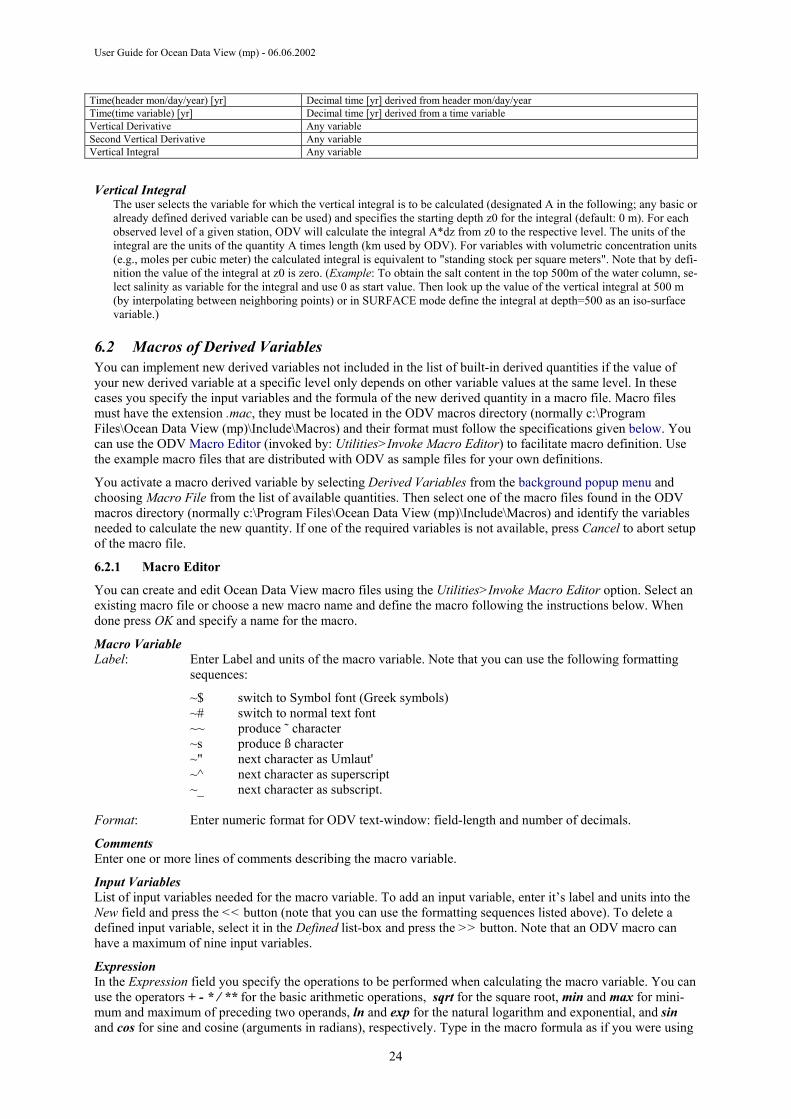
Time(header mon/day/year) [yr] Decimal time [yr] derived from header mon/day/year Time(time variable) [yr] Decimal time [yr] derived from a time variable Vertical Derivative Any variable Second Vertical Derivative Any variable Vertical Integral Any variable
Vertical Integral The user selects the variable for which the vertical integral is to be calculated (designated A in the following; any basic or already defined derived variable can be used) and specifies the starting depth z0 for the integral (default: 0 m). For each observed level of a given station, ODV will calculate the integral A*dz from z0 to the respective level. The units of the integral are the units of the quantity A times length (km used by ODV). For variables with volumetric concentration units (e.g., moles per cubic meter) the calculated integral is equivalent to "standing stock per square meters". Note that by defi-nition the value of the integral at z0 is zero. (Example: To obtain the salt content in the top 500m of the water column, se-lect salinity as variable for the integral and use 0 as start value. Then look up the value of the vertical integral at 500 m (by interpolating between neighboring points) or in SURFACE mode define the integral at depth=500 as an iso-surface variable.)
6.2 Macros of Derived Variables You can implement new derived variables not included in the list of built-in derived quantities if the value of your new derived variable at a specific level only depends on other variable values at the same level. In these cases you specify the input variables and the formula of the new derived quantity in a macro file. Macro files must have the extension .mac, they must be located in the ODV macros directory (normally c:\Program Files\Ocean Data View (mp)\Include\Macros) and their format must follow the specifications given below. You can use the ODV Macro Editor (invoked by: Utilities>Invoke Macro Editor) to facilitate macro definition. Use the example macro files that are distributed with ODV as sample files for your own definitions.
You activate a macro derived variable by selecting Derived Variables from the background popup menu and choosing Macro File from the list of available quantities. Then select one of the macro files found in the ODV macros directory (normally c:\Program Files\Ocean Data View (mp)\Include\Macros) and identify the variables needed to calculate the new quantity. If one of the required variables is not available, press Cancel to abort setup of the macro file.
6.2.1 Macro Editor
You can create and edit Ocean Data View macro files using the Utilities>Invoke Macro Editor option. Select an existing macro file or choose a new macro name and define the macro following the instructions below. When done press OK and specify a name for the macro.
Macro Variable Label: Enter Label and units of the macro variable. Note that you can use the following formatting
sequences:
~$ switch to Symbol font (Greek symbols) ~# switch to normal text font ~~ produce ˜ character ~s produce ß character ~" next character as Umlaut' ~^ next character as superscript ~_ next character as subscript.
Format: Enter numeric format for ODV text-window: field-length and number of decimals.
Comments Enter one or more lines of comments describing the macro variable.
Input Variables List of input variables needed for the macro variable. To add an input variable, enter it’s label and units into the New field and press the << button (note that you can use the formatting sequences listed above). To delete a defined input variable, select it in the Defined list-box and press the >> button. Note that an ODV macro can have a maximum of nine input variables.
Expression In the Expression field you specify the operations to be performed when calculating the macro variable. You can use the operators + - * / ** for the basic arithmetic operations, sqrt for the square root, min and max for mini-mum and maximum of preceding two operands, ln and exp for the natural logarithm and exponential, and sin and cos for sine and cosine (arguments in radians), respectively. Type in the macro formula as if you were using
24
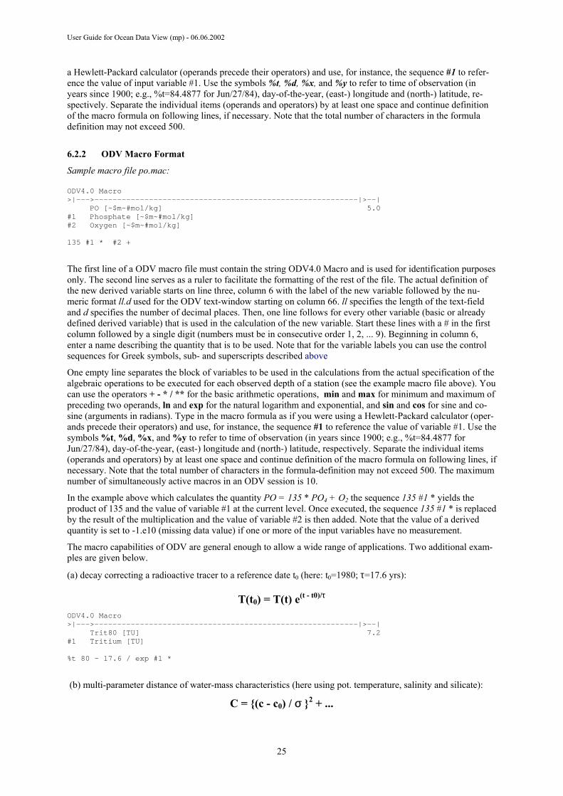
User Guide for Ocean Data View (mp) - 06.06.2002
a Hewlett-Packard calculator (operands precede their operators) and use, for instance, the sequence #1 to refer-ence the value of input variable #1. Use the symbols %t, %d, %x, and %y to refer to time of observation (in years since 1900; e.g., %t=84.4877 for Jun/27/84), day-of-the-year, (east-) longitude and (north-) latitude, re-spectively. Separate the individual items (operands and operators) by at least one space and continue definition of the macro formula on following lines, if necessary. Note that the total number of characters in the formula definition may not exceed 500.
6.2.2 ODV Macro Format
Sample macro file po.mac:
ODV4.0 Macro>|--->----------------------------------------------------------|>--|
PO [~$m~#mol/kg] 5.0#1 Phosphate [~$m~#mol/kg]#2 Oxygen [~$m~#mol/kg]
135 #1 * #2 +
The first line of a ODV macro file must contain the string ODV4.0 Macro and is used for identification purposes only. The second line serves as a ruler to facilitate the formatting of the rest of the file. The actual definition of the new derived variable starts on line three, column 6 with the label of the new variable followed by the nu-meric format ll.d used for the ODV text-window starting on column 66. ll specifies the length of the text-field and d specifies the number of decimal places. Then, one line follows for every other variable (basic or already defined derived variable) that is used in the calculation of the new variable. Start these lines with a # in the first column followed by a single digit (numbers must be in consecutive order 1, 2, ... 9). Beginning in column 6, enter a name describing the quantity that is to be used. Note that for the variable labels you can use the control sequences for Greek symbols, sub- and superscripts described above
One empty line separates the block of variables to be used in the calculations from the actual specification of the algebraic operations to be executed for each observed depth of a station (see the example macro file above). You can use the operators + - * / ** for the basic arithmetic operations, min and max for minimum and maximum of preceding two operands, ln and exp for the natural logarithm and exponential, and sin and cos for sine and co-sine (arguments in radians). Type in the macro formula as if you were using a Hewlett-Packard calculator (oper-ands precede their operators) and use, for instance, the sequence #1 to reference the value of variable #1. Use the symbols %t, %d, %x, and %y to refer to time of observation (in years since 1900; e.g., %t=84.4877 for Jun/27/84), day-of-the-year, (east-) longitude and (north-) latitude, respectively. Separate the individual items (operands and operators) by at least one space and continue definition of the macro formula on following lines, if necessary. Note that the total number of characters in the formula-definition may not exceed 500. The maximum number of simultaneously active macros in an ODV session is 10.
In the example above which calculates the quantity PO = 135 * PO4 + O2 the sequence 135 #1 * yields the product of 135 and the value of variable #1 at the current level. Once executed, the sequence 135 #1 * is replaced by the result of the multiplication and the value of variable #2 is then added. Note that the value of a derived quantity is set to -1.e10 (missing data value) if one or more of the input variables have no measurement.
The macro capabilities of ODV are general enough to allow a wide range of applications. Two additional exam-ples are given below.
(a) decay correcting a radioactive tracer to a reference date t0 (here: t0=1980; τ=17.6 yrs):
T(t0) = T(t) e(t - t0)/τ ODV4.0 Macro>|--->----------------------------------------------------------|>--|
Trit80 [TU] 7.2#1 Tritium [TU]
%t 80 - 17.6 / exp #1 *
(b) multi-parameter distance of water-mass characteristics (here using pot. temperature, salinity and silicate):
C = {(c - c0) / σ }2 + ...
25

User Guide for Ocean Data View (mp) - 06.06.2002
ODV4.0 Macro>|--->----------------------------------------------------------|>--|
MP-Dist{10,34.7,25} 7.0#1 Tpot [C]#2 Salinity [psu]#3 Silicate [umol/kg]
#1 10 - 0.1 / 2 **#2 34.7 - 0.05 / 2 ** +#3 25 - 0.5 / 2 ** +
6.3 Expressions Expressions are similar to macros, they use the same function set and are defined in roughly the same way. The main difference is that the definition of an expression is not recorded in a file and expressions cannot be edited. Expressions are ideal for checking out newly devised derived quantities quickly. The scope of an expression is limited to the collection for which it is defined. If an expression is complicated or if you want to use the same expression with many different collections, you should create a macro file instead.
To setup an expression derived variable select Derived Variables from the background popup menu, choose Expression from the list of available quantities and press Add. ODV will show a dialog similar to the macro editor dialog. You should enter the label of the new variable and the corresponding units in the Label field. Then select the input variables required by the new variable, e.g., select a variable in the Choices list and press <-. Finally, specify the expression to be evaluated for the new quantity. You can use the operators + - * / ** for the basic arithmetic operations, min and max for minimum and maximum of preceding two operands, ln and exp for the natural logarithm and exponential, and sin and cos for sine and cosine (arguments in radians). Type in the macro formula as if you were using a Hewlett-Packard calculator (operands precede their operators) and use, for instance, the sequence #1 to reference the value of the first input variable #1. Use the symbols %t, %d, %x, and %y to refer to time of observation (in years since 1900; e.g., %t=84.4877 for Jun/27/84), day-of-the-year, (east-) longitude and (north-) latitude, respectively. Separate the individual items (operands and operators) by at least one space and continue definition of the macro formula on following lines, if necessary. Note that the total num-ber of characters in the formula-definition may not exceed 500. Press OK to finish the setup of the new expres-sion.
Note that expressions can not be edited. If you want to modify the algorithm you have to delete the old expres-sion variable and define a new one.
26

User Guide for Ocean Data View (mp) - 06.06.2002
7 Using ODV
7.1 Choosing Current Sample and Current Station When ODV has opened a collection and has drawn the station map, one of the valid stations shown in the map is the current station. This station is marked by a red circle and the header as well as data information appear in ODV’s text window. There are several different ways to select a new current station:
(1) click the left mouse button on any station in the map. To be able to select amongst multiple stations at the same position (repeat stations, mooring instruments, etc.) hold down the SHIFT key while clicking the left mouse button. ODV then presents a list of matching stations and lets you select one entry from the list. Without the SHIFT key, the first matching station is selected by default.
(2) choose Select Station by Name from the map popup menu and specific cruise label, station label and sta-tion type.
(3) choose Select Station by Number from the map popup menu (or simply press #) and specify the internal sequence number of the station.
Pressing the right arrow key (->) advances to the next valid station, pressing the left arrow key (<-) gets you to the previous one. One of the samples of the current station is the current sample, and the data values of this sample are listed in line 3 of ODV’s text window. If data plots are on the screen the current sample is also marked by red cross hairs in each of the plots. You can select deeper or shallower new samples of the same station by pressing the up/down and PgUp/PgDn arrow-keys, or you can make any data point in any of the data plots the current sample by sim-ply clicking on it with the left mouse button.
If you move the mouse over lines 2 and 3 of the text window you get more detailed information on the data value, including its quality flag. You can change the numeric format and order in which the variables are listed in the text window by choosing Variables Settings from the text-window popup menu.
7.2 Changing Variable Settings You can modify the variable labels, the default min/max ranges, the numeric format and the position in line 3 of ODV’s text-window for any collection variable using the Variables Settings option of the text window popup menu (click right mouse button while over the text window and select Variables Settings).
First select a variable that you want to modify using the Variable control (if the mouse was over the respective variable when you right-clicked, this variable is already pre-selected). Then modify the different properties for this variable. You change the variable label and units string by editing the Label item. Note that the units should be enclosed between [ and ] brackets. You change the default lower and upper value ranges of the variable by setting the Minimum and Maximum entries. You modify the numeric format used to list data for the variable in line 3 of the text window by setting the Format entries. The first number specifies the length of the field (in characters) and the second number specifies the number of decimal places. Finally, you can change the position of the variable in the text window using the Position combo-box (select the new position of the variable, e.g. potential temperature next to (in-situ) temperature). Continue making changes for other variables (select them using the Variable combo-box) and press OK when you are done.
27
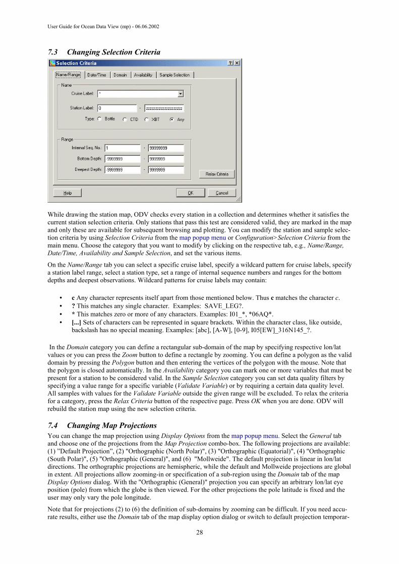
User Guide for Ocean Data View (mp) - 06.06.2002
7.3 Changing Selection Criteria
While drawing the station map, ODV checks every station in a collection and determines whether it satisfies the current station selection criteria. Only stations that pass this test are considered valid, they are marked in the map and only these are available for subsequent browsing and plotting. You can modify the station and sample selec-tion criteria by using Selection Criteria from the map popup menu or Configuration>Selection Criteria from the main menu. Choose the category that you want to modify by clicking on the respective tab, e.g., Name/Range, Date/Time, Availability and Sample Selection, and set the various items.
On the Name/Range tab you can select a specific cruise label, specify a wildcard pattern for cruise labels, specify a station label range, select a station type, set a range of internal sequence numbers and ranges for the bottom depths and deepest observations. Wildcard patterns for cruise labels may contain:
• c Any character represents itself apart from those mentioned below. Thus c matches the character c. • ? This matches any single character. Examples: SAVE_LEG?. • * This matches zero or more of any characters. Examples: I01_*, *06AQ*. • [...] Sets of characters can be represented in square brackets. Within the character class, like outside,
backslash has no special meaning. Examples: [abc], [A-W], [0-9], I05[EW]_316N145_?.
In the Domain category you can define a rectangular sub-domain of the map by specifying respective lon/lat values or you can press the Zoom button to define a rectangle by zooming. You can define a polygon as the valid domain by pressing the Polygon button and then entering the vertices of the polygon with the mouse. Note that the polygon is closed automatically. In the Availability category you can mark one or more variables that must be present for a station to be considered valid. In the Sample Selection category you can set data quality filters by specifying a value range for a specific variable (Validate Variable) or by requiring a certain data quality level. All samples with values for the Validate Variable outside the given range will be excluded. To relax the criteria for a category, press the Relax Criteria button of the respective page. Press OK when you are done. ODV will rebuild the station map using the new selection criteria.
7.4 Changing Map Projections You can change the map projection using Display Options from the map popup menu. Select the General tab and choose one of the projections from the Map Projection combo-box. The following projections are available: (1) ”Default Projection”, (2) "Orthographic (North Polar)", (3) "Orthographic (Equatorial)", (4) "Orthographic (South Polar)", (5) "Orthographic (General)", and (6) "Mollweide". The default projection is linear in lon/lat directions. The orthographic projections are hemispheric, while the default and Mollweide projections are global in extent. All projections allow zooming-in or specification of a sub-region using the Domain tab of the map Display Options dialog. With the "Orthographic (General)" projection you can specify an arbitrary lon/lat eye position (pole) from which the globe is then viewed. For the other projections the pole latitude is fixed and the user may only vary the pole longitude.
Note that for projections (2) to (6) the definition of sub-domains by zooming can be difficult. If you need accu-rate results, either use the Domain tab of the map display option dialog or switch to default projection temporar-
28

User Guide for Ocean Data View (mp) - 06.06.2002
ily, then zoom (thereby defining the sub-region) and finally switch back to the desired map projection.
For a description of other map display options see Changing Display Options.
7.5 Full Screen Station Maps You can produce full-screen station maps by choosing MAP Mode from the background popup menu. You can label a station in the map by double clicking on it, and you can remove the annotation of the current station by pressing the delete button (Del or Entf). Note that the positioning of the annotation depends on the mouse posi-tion at the time of the double-click relative to the station position. Try it. You change the annotation style and font-size through Display Options dialog box. You can produce a hardcopy of the station map through File>Print or you can obtain a PostScript, PNG or JPG file of the map using File>Save As from the main menu and selecting the desired format.
29
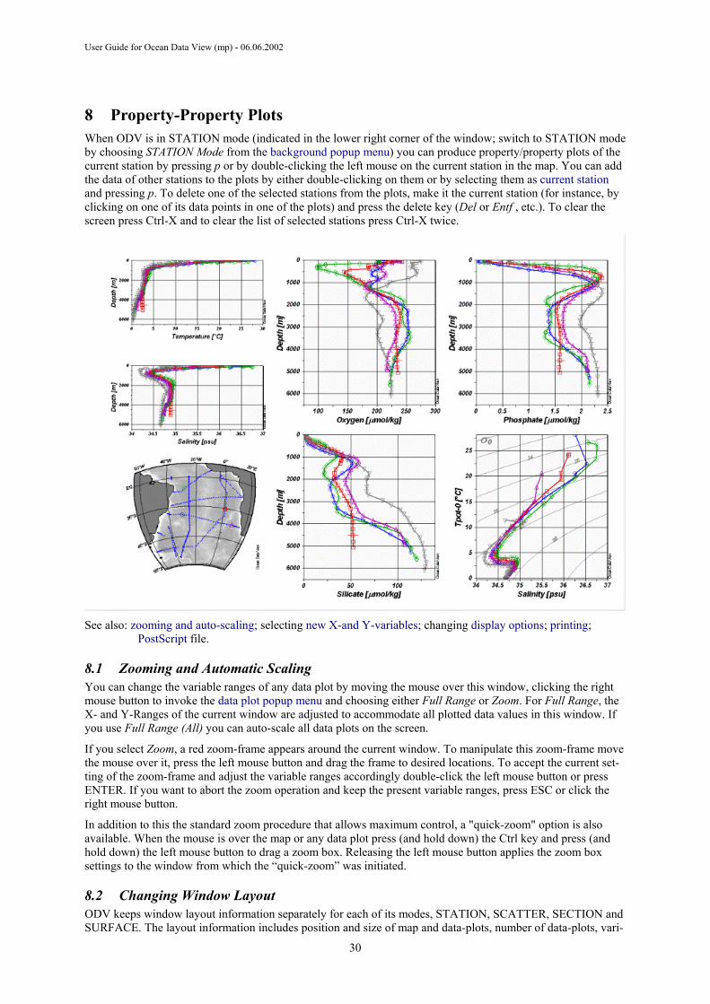
User Guide for Ocean Data View (mp) - 06.06.2002
8 Property-Property Plots When ODV is in STATION mode (indicated in the lower right corner of the window; switch to STATION mode by choosing STATION Mode from the background popup menu) you can produce property/property plots of the current station by pressing p or by double-clicking the left mouse on the current station in the map. You can add the data of other stations to the plots by either double-clicking on them or by selecting them as current station and pressing p. To delete one of the selected stations from the plots, make it the current station (for instance, by clicking on one of its data points in one of the plots) and press the delete key (Del or Entf , etc.). To clear the screen press Ctrl-X and to clear the list of selected stations press Ctrl-X twice.
See also: zooming and auto-scaling; selecting new X-and Y-variables; changing display options; printing;
PostScript file.
8.1 Zooming and Automatic Scaling You can change the variable ranges of any data plot by moving the mouse over this window, clicking the right mouse button to invoke the data plot popup menu and choosing either Full Range or Zoom. For Full Range, the X- and Y-Ranges of the current window are adjusted to accommodate all plotted data values in this window. If you use Full Range (All) you can auto-scale all data plots on the screen.
If you select Zoom, a red zoom-frame appears around the current window. To manipulate this zoom-frame move the mouse over it, press the left mouse button and drag the frame to desired locations. To accept the current set-ting of the zoom-frame and adjust the variable ranges accordingly double-click the left mouse button or press ENTER. If you want to abort the zoom operation and keep the present variable ranges, press ESC or click the right mouse button.
In addition to this the standard zoom procedure that allows maximum control, a "quick-zoom" option is also available. When the mouse is over the map or any data plot press (and hold down) the Ctrl key and press (and hold down) the left mouse button to drag a zoom box. Releasing the left mouse button applies the zoom box settings to the window from which the “quick-zoom” was initiated.
8.2 Changing Window Layout ODV keeps window layout information separately for each of its modes, STATION, SCATTER, SECTION and SURFACE. The layout information includes position and size of map and data-plots, number of data-plots, vari-
30
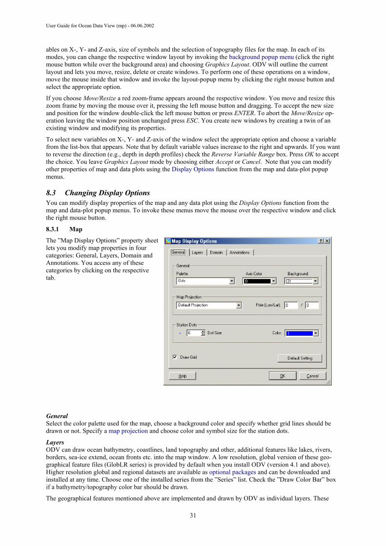
User Guide for Ocean Data View (mp) - 06.06.2002
ables on X-, Y- and Z-axis, size of symbols and the selection of topography files for the map. In each of its modes, you can change the respective window layout by invoking the background popup menu (click the right mouse button while over the background area) and choosing Graphics Layout. ODV will outline the current layout and lets you move, resize, delete or create windows. To perform one of these operations on a window, move the mouse inside that window and invoke the layout-popup menu by clicking the right mouse button and select the appropriate option.
If you choose Move/Resize a red zoom-frame appears around the respective window. You move and resize this zoom frame by moving the mouse over it, pressing the left mouse button and dragging. To accept the new size and position for the window double-click the left mouse button or press ENTER. To abort the Move/Resize op-eration leaving the window position unchanged press ESC. You create new windows by creating a twin of an existing window and modifying its properties.
To select new variables on X-, Y- and Z-axis of the window select the appropriate option and choose a variable from the list-box that appears. Note that by default variable values increase to the right and upwards. If you want to reverse the direction (e.g., depth in depth profiles) check the Reverse Variable Range box. Press OK to accept the choice. You leave Graphics Layout mode by choosing either Accept or Cancel. Note that you can modify other properties of map and data plots using the Display Options function from the map and data-plot popup menus.
8.3 Changing Display Options You can modify display properties of the map and any data plot using the Display Options function from the map and data-plot popup menus. To invoke these menus move the mouse over the respective window and click the right mouse button.
8.3.1 Map
The ”Map Display Options” property sheet lets you modify map properties in four categories: General, Layers, Domain and Annotations. You access any of these categories by clicking on the respective tab.
General Select the color palette used for the map, choose a background color and specify whether grid lines should be drawn or not. Specify a map projection and choose color and symbol size for the station dots.
Layers ODV can draw ocean bathymetry, coastlines, land topography and other, additional features like lakes, rivers, borders, sea-ice extend, ocean fronts etc. into the map window. A low resolution, global version of these geo-graphical feature files (GlobLR series) is provided by default when you install ODV (version 4.1 and above). Higher resolution global and regional datasets are available as optional packages and can be downloaded and installed at any time. Choose one of the installed series from the ”Series” list. Check the ”Draw Color Bar” box if a bathymetry/topography color bar should be drawn.
The geographical features mentioned above are implemented and drawn by ODV as individual layers. These
31
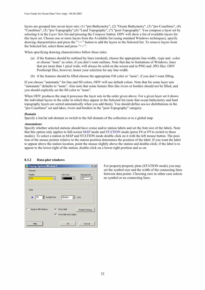
User Guide for Ocean Data View (mp) - 06.06.2002
layers are grouped into seven layer sets: (1) "pre-Bathymetry", (2) "Ocean Bathymetry", (3) "pre-Coastlines", (4) "Coastlines", (5) "pre-Topography",(6) "Land Topography", (7) "post-Topography". You compose a layer set by selecting it in the Layer Sets list and pressing the Compose button. ODV will show a list of available layers for this layer set. Choose one or more layers from the Available list (using standard Windows techniques), specify drawing characteristics and press the ”<<” button to add the layers to the Selected list. To remove layers from the Selected list, select them and press ”>>”.
When specifying drawing characteristics follow these rules:
(a) if the features should be outlined by lines (stroked), choose the appropriate line-width, -type and –color or choose ”none” as color, if you don’t want outlines. Note that due to limitations of Windows, lines that are more than 1 pixel wide, will always be solid on the screen and in PNG and .JPG files. ODV PostScript files, however, honor your selection for any line-width.
(b) if the features should be filled choose the appropriate Fill color or ”none”, if you don’t want filling.
If you choose ”automatic” for line and fill colors, ODV will use default colors. Note that for some layer sets ”automatic” defaults to ”none”. Also note that some feature files like rivers or borders should not be filled, and you should explicitly set the fill color to ”none”.
When ODV produces the map it processes the layer sets in the order given above. For a given layer set it draws the individual layers in the order in which they appear in the Selected list (note that ocean bathymetry and land topography layers are sorted automatically when you add them). You should define sea-ice distributions in the "pre-Coastlines" set and lakes, rivers and borders in the "post-Topography" category.
Domain Specify a lon/lat sub-domain or switch to the full domain of the collection or to a global map.
Annotations Specify whether selected stations should have cruise and/or station labels and set the font size of the labels. Note that this option only applies to full-screen MAP mode and STATION mode (press F8 or F9 to switch to these modes). To select a station in MAP and STATION mode double click on it with the left mouse button. The posi-tion of the mouse pointer relative to the station position determines the position of the label. If you want the label to appear above the station location, point the mouse slightly above the station and double-click; if the label is to appear to the lower-right of the station, double-click on a lower-right position and so on.
8.3.2 Data-plot windows
For property/property plots (STATION mode) you may set the symbol-size and the width of the connecting lines between data points. Choosing zero in either case selects no symbol or no connecting lines.
32

User Guide for Ocean Data View (mp) - 06.06.2002
For scatter, section or surface plots (SCATTER, SECTION and SURFACE modes) you can set the display mode (Original Data: colored dots, numeric values or arrows; Quick Gridding; VG Gridding), the dot (or font) size for the original data, the point-size (for scatter plots), and the X- and Y- averaging length scales for gridded fields. Note that two different grid-ding algorithms are available and that contouring is supported for both. Also note that the X- and Y- length scales are measured in per mille of the respective axis range and that large values result in smooth fields. You should try different settings for the length-scales and select the ones that you like most.
Uncheck the Automatic Axis Labels box if you want to switch off the automatic generation of axis labels and place annotations manually. If the Apply to All Win-dows box is checked the modifications that you make will apply to all data plots in the current mode. If you want to establish individual styles for your data plots, make sure this box is not checked. For gridded fields, use the Properties button to set additional options and to specify contour lines (see below).
On the Properties dialog you can
• set additional general options, • switch on/off color shading, • switch on/off automatic removal of outliers (compu-
tationally expensive), • specify contour lines.
To add sets of contour lines specify Start, Increment and End values in the New group. Choose appropriate line-styles and colors and set the Label Size entry. Then press the << button to add the respective set of contour lines. You can repeat this procedure with different Start, Incre-ment and End values and possibly different line proper-ties. Note that the maximum number of contour lines per window is 50. To modify the properties of an existing contour line, select it in the Already Defined list, modify the properties in the New group and press << to imple-ment the changes.
8.4 Printing Choose Print from the File or background popup menus to print the contents of the current ODV graphics win-dow.
WIN32 ODV invokes a standard Windows print-dialog box and lets you select one of the printers available on your system. Press OK to start the printing. Note that print jobs for complicated screen graphics tend to be large and time-consuming. If you have access to a PostScript printer, use the PostScript option instead.
UNIX Not tested.
33
User Guide for Ocean Data View (mp) - 06.06.2002
8.5 PostScript Files To produce PostScript versions of the entire screen or of individual plots choose the Save As option of the entire screen or of an individual plot (e.g., by right-clicking on the background or respective data plot and choosing Save As or Extras>Save Single As; alternatively, press CTRL-S while over the background or data plot) and choose PostScript (*.eps) as file-type. You can then specify the orientation of output, set scaling parameters and choose the pathname of the output file.
The resulting PostScript file can be printed by sending it to a PostScript printer or it can be imported into LaTex, Word, PageMaker and other page-design documents (to use this feature, you should save the plot in Portrait orientation).
While Print jobs tend to be large for complicated section and surface plots, the PostScript files are much tighter and printing may be faster. Note that by default the PostScript files are written to ODV’s Temporary Files direc-tory and that the file-name is derived from the current configuration name. You can choose any other file name or destination directory using the Windows File Save dialog that appears automatically.
8.6 PNG and JPG Files You can export the current ODV graphics screen or individual data plots in PNG or JPG files (use PNG for in-clusion in text documents or post-processing with standard graphics software) by choosing Save As from the background popup menu (ODV screen) or Extras>Save Single As from a data plot popup menu (individual plot). Note that you can reach these options via shortcut key-strokes: (1) pressing Ctrl-S while the mouse is over the background area produces a full ODV screen representation while (2) pressing Ctrl-S with the mouse over a data plot will produce a version of the respective data plot. ODV will present a file-save dialog box and you should choose the appropriate output file-type (PNG (*.PNG) or JPG (*.JPG)). Note that the default name of PNG or JPG files is derived from the current configuration name, but you can choose any other name or destination.
Also note that PNG files by definition only support up to 256 colors. If you use different palettes for the individ-ual data plot windows, only the palette of the last plot window is displayed correctly in the PNG file, and false colors may appear in the other windows. In these cases you should use the JPG (*.JPG) output format instead of PNG, or you should produce separate PNG files for the individual data plot windows (option Extras>Save Single As of the data plot popup menu).
34

User Guide for Ocean Data View (mp) - 06.06.2002
9 Scatter Plots
9.1 Producing Scatter Plots You can produce property/property plots of all data of all currently valid stations (optionally colored using a third variable) by switching to ODV’s SCATTER Mode (using the background popup menu) and double-clicking the left mouse button on the map.
See also: zooming and auto-scaling; selecting new X-and Y-variables; changing display options; printing;
PostScript file.
35
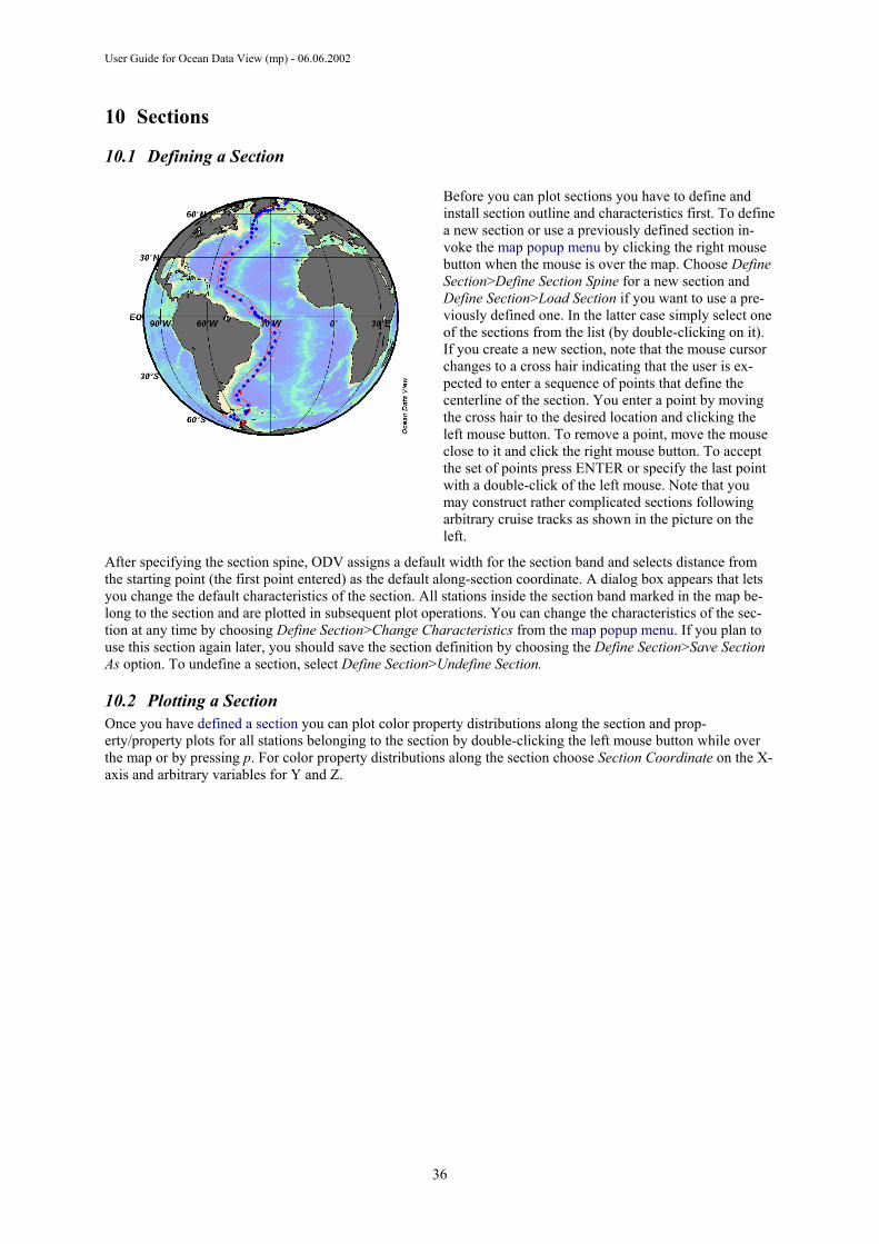
User Guide for Ocean Data View (mp) - 06.06.2002
10 Sections
10.1 Defining a Section
Before you can plot sections you have to define and install section outline and characteristics first. To define a new section or use a previously defined section in-voke the map popup menu by clicking the right mouse button when the mouse is over the map. Choose Define Section>Define Section Spine for a new section and Define Section>Load Section if you want to use a pre-viously defined one. In the latter case simply select one of the sections from the list (by double-clicking on it). If you create a new section, note that the mouse cursor changes to a cross hair indicating that the user is ex-pected to enter a sequence of points that define the centerline of the section. You enter a point by moving the cross hair to the desired location and clicking the left mouse button. To remove a point, move the mouse close to it and click the right mouse button. To accept the set of points press ENTER or specify the last point with a double-click of the left mouse. Note that you may construct rather complicated sections following arbitrary cruise tracks as shown in the picture on the left.
After specifying the section spine, ODV assigns a default width for the section band and selects distance from the starting point (the first point entered) as the default along-section coordinate. A dialog box appears that lets you change the default characteristics of the section. All stations inside the section band marked in the map be-long to the section and are plotted in subsequent plot operations. You can change the characteristics of the sec-tion at any time by choosing Define Section>Change Characteristics from the map popup menu. If you plan to use this section again later, you should save the section definition by choosing the Define Section>Save Section As option. To undefine a section, select Define Section>Undefine Section.
10.2 Plotting a Section Once you have defined a section you can plot color property distributions along the section and prop-erty/property plots for all stations belonging to the section by double-clicking the left mouse button while over the map or by pressing p. For color property distributions along the section choose Section Coordinate on the X-axis and arbitrary variables for Y and Z.
36

User Guide for Ocean Data View (mp) - 06.06.2002
See also: zooming and auto-scaling; color-zooming; changing the color mapping function; selecting new X, Y-
and Z-variables; changing display options; displaying gridded fields; values; printing; PostScript file.
10.3 Color-Zooming Color section plots and color distributions on iso-surfaces allow modifications of the Z-variable ranges by color zooming. To invoke color-zooming move the mouse over the section or iso-surface plot that you want to modify and click the right mouse button to bring up the data plot popup menu. Selecting Z-Zoom will draw a red zoom-frame around the color bar of the respective window. Manipulate and drag this zoom-frame as described above. To accept the current setting of the zoom-frame and adjust the Z-variable range accordingly double-click the left mouse button or press ENTER. If you want to abort the zoom operation and keep the present variable range, press ESC or click the right mouse button.
37
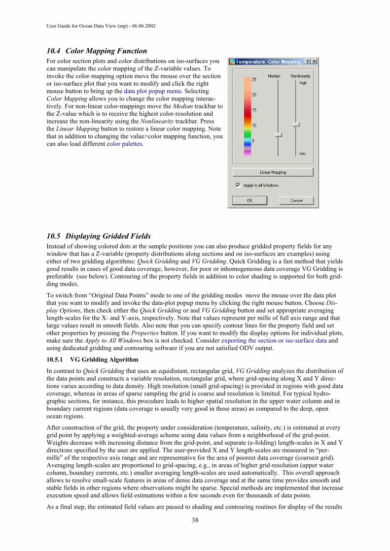
User Guide for Ocean Data View (mp) - 06.06.2002
10.4 Color Mapping Function For color section plots and color distributions on iso-surfaces you can manipulate the color mapping of the Z-variable values. To invoke the color-mapping option move the mouse over the section or iso-surface plot that you want to modify and click the right mouse button to bring up the data plot popup menu. Selecting Color Mapping allows you to change the color mapping interac-tively. For non-linear color-mappings move the Median trackbar to the Z-value which is to receive the highest color-resolution and increase the non-linearity using the Nonlinearity trackbar. Press the Linear Mapping button to restore a linear color mapping. Note that in addition to changing the value>color mapping function, you can also load different color palettes.
10.5 Displaying Gridded Fields Instead of showing colored dots at the sample positions you can also produce gridded property fields for any window that has a Z-variable (property distributions along sections and on iso-surfaces are examples) using either of two gridding algorithms: Quick Gridding and VG Gridding. Quick Gridding is a fast method that yields good results in cases of good data coverage, however, for poor or inhomogeneous data coverage VG Gridding is preferable (see below). Contouring of the property fields in addition to color shading is supported for both grid-ding modes.
To switch from “Original Data Points” mode to one of the gridding modes move the mouse over the data plot that you want to modify and invoke the data-plot popup menu by clicking the right mouse button. Choose Dis-play Options, then check either the Quick Gridding or and VG Gridding button and set appropriate averaging length-scales for the X- and Y-axis, respectively. Note that values represent per mille of full axis range and that large values result in smooth fields. Also note that you can specify contour lines for the property field and set other properties by pressing the Properties button. If you want to modify the display options for individual plots, make sure the Apply to All Windows box is not checked. Consider exporting the section or iso-surface data and using dedicated gridding and contouring software if you are not satisfied ODV output.
10.5.1 VG Gridding Algorithm
In contrast to Quick Gridding that uses an equidistant, rectangular grid, VG Gridding analyzes the distribution of the data points and constructs a variable resolution, rectangular grid, where grid-spacing along X and Y direc-tions varies according to data density. High resolution (small grid-spacing) is provided in regions with good data coverage, whereas in areas of sparse sampling the grid is coarse and resolution is limited. For typical hydro-graphic sections, for instance, this procedure leads to higher spatial resolution in the upper water column and in boundary current regions (data coverage is usually very good in these areas) as compared to the deep, open ocean regions.
After construction of the grid, the property under consideration (temperature, salinity, etc.) is estimated at every grid point by applying a weighted-average scheme using data values from a neighborhood of the grid-point. Weights decrease with increasing distance from the grid-point, and separate (e-folding) length-scales in X and Y directions specified by the user are applied. The user-provided X and Y length-scales are measured in “per-mille” of the respective axis range and are representative for the area of poorest data coverage (coarsest grid). Averaging length-scales are proportional to grid-spacing, e.g., in areas of higher grid-resolution (upper water column, boundary currents, etc.) smaller averaging length-scales are used automatically. This overall approach allows to resolve small-scale features in areas of dense data coverage and at the same time provides smooth and stable fields in other regions where observations might be sparse. Special methods are implemented that increase execution speed and allows field estimations within a few seconds even for thousands of data points.
As a final step, the estimated field values are passed to shading and contouring routines for display of the results
38
User Guide for Ocean Data View (mp) - 06.06.2002
on the screen or on a printer.
10.6 Difference Fields You can compare property distributions of the currently selected stations with previously saved reference data and produce difference fields by defining property differences as derived variables. Choose Derived Variables from ODV’s background menu (or press Alt+D) and select Diff. from Ref. Choose the ExportID.txt file of the reference data that you want to use in one of the subdirectories of Temp\Reference. ODV will show a list of available reference data files from that directory. Select an .oal file that has the variable for which you want to produce the difference field as Z variable and appropriate X and Y variables (e.g., for producing longitude vs. depth sections, make sure the reference data file has longitude as X and depth as Y variable). Now identify the Z, X and Y variables in the current collection (if longitude or latitude are required, define them as derived variables prior to invoking Diff. from Ref.) to complete the definition of the difference variable. Note that the name of the new variable is composed of the name of the Z variable and the identification string of the reference data set. Once defined, you can use the difference variable in any data plot.
39
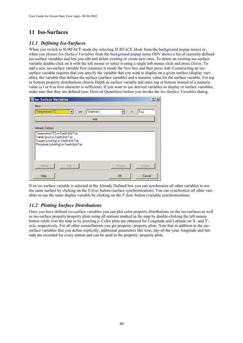
User Guide for Ocean Data View (mp) - 06.06.2002
11 Iso-Surfaces
11.1 Defining Iso-Surfaces When you switch to SURFACE mode (by selecting SURFACE Mode from the background popup menu) or when you choose Iso-Surface Variables from the background popup menu ODV shows a list of currently defined iso-surface variables and lets you edit and delete existing or create new ones. To delete an existing iso-surface variable double-click on it with the left mouse or select it using a single left mouse click and press Delete. To add a new iso-surface variable first construct it inside the New box and then press Add. Constructing an iso-surface variable requires that you specify the variable that you want to display on a given surface (display vari-able), the variable that defines the surface (surface variable) and a numeric value for the surface variable. For top or bottom property distributions choose Depth as surface variable and enter top or bottom instead of a numeric value (a t or b as first character is sufficient). If you want to use derived variables as display or surface variables, make sure that they are defined (see: Derived Quantities) before you invoke the Iso-Surface Variables dialog.
If an iso-surface variable is selected in the Already Defined box you can synchronize all other variables to use the same surface by clicking on the S-Sync button (surface synchronization). You can synchronize all other vari-ables to use the same display variable by clicking on the V-Sync button (variable synchronization).
11.2 Plotting Surface Distributions Once you have defined iso-surface variables you can plot color property distributions on the iso-surfaces as well as iso-surface property/property plots using all stations marked in the map by double-clicking the left mouse button while over the map or by pressing p. Color plots are obtained for Longitude and Latitude on X- and Y-axis, respectively. For all other constellations you get property/ property plots. Note that in addition to the iso-surface variables that you define explicitly, additional parameters like time, day-of-the-year, longitude and lati-tude are recorded for every station and can be used in the property/ property plots.
40

User Guide for Ocean Data View (mp) - 06.06.2002
See also: zooming and auto-scaling; color-zooming; changing the color mapping function; selecting new X, Y-
and Z-variables; changing display options; displaying gridded fields; values; printing; PostScript file.
41
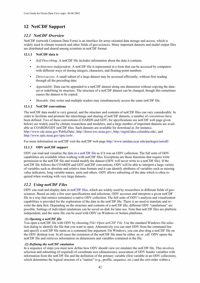
User Guide for Ocean Data View (mp) - 06.06.2002
12 NetCDF Support
12.1 NetCDF Overview NetCDF (network Common Data Form) is an interface for array-oriented data storage and access, which is widely used in climate research and other fields of geo-sciences. Many important datasets and model output files are distributed and shared among scientists in netCDF format.
12.1.1 NetCDF data is
• Self-Describing. A netCDF file includes information about the data it contains.
• Architecture-independent. A netCDF file is represented in a form that can be accessed by computers with different ways of storing integers, characters, and floating-point numbers.
• Direct-access. A small subset of a large dataset may be accessed efficiently, without first reading through all the preceding data.
• Appendable. Data can be appended to a netCDF dataset along one dimension without copying the data-set or redefining its structure. The structure of a netCDF dataset can be changed, though this sometimes causes the dataset to be copied.
• Sharable. One writer and multiple readers may simultaneously access the same netCDF file.
12.1.2 NetCDF conventions
The netCDF data model is very general, and the structure and contents of netCDF files can vary considerably. In order to facilitate and promote the interchange and sharing of netCDF datasets, a number of conventions have been defined. Two of these conventions (COARDS and GDT; for specifications see netCDF web page given below) are widely used by climate researchers and modelers, and a large number of important datasets are avail-able as COARDS/GDT netCDF files. Such datasets are available for download at, for instance, http://www.cdc.noaa.gov/PublicData/, http://ferret.wrc.noaa.gov/, http://ingrid.ldeo.columbia.edu/, and http://www.epic.noaa.gov/epic/ewb/.
For more information on netCDF visit the netCDF web page http://www.unidata.ucar.edu/packages/netcdf/.
12.1.3 ODV netCDF support
ODV can read and visualize the data in a netCDF file as if it was an ODV collection. The full suite of ODV capabilities are available when working with netCDF files. Exceptions are those functions that require write permission to the netCDF file and would modify the dataset (ODV will never write to a netCDF file). If the netCDF file follows the COARDS and GDT netCDF conventions, ODV will be able to interpret a large variety of variables such as absolute and relative time formats and it can identify attributes of variables such as missing value indicators, long variable names, units and others. ODV allows subsetting of the data which is often re-quired when working with very large datasets.
12.2 Using netCDF Files ODV can read and display data in netCDF files, which are widely used by researchers in different fields of geo-sciences. Based on only a few user specifications and selections, ODV accesses and interprets a given netCDF file in a way that mimics (emulates) a native ODV collection. The full suite of ODV’s analysis and visualization capabilities is provided for the exploration of the data in the netCDF file. There is no need to translate and re-write the data first. Depending on the structure and contents of a netCDF file, different ODV “emulations” are possible. Settings of individual emulations can be saved on disk for later use. Note that netCDF files are platform independent, and the same file can be used with ODV on Windows or Solaris platforms.
(1) Opening a netCDF file You open a netCDF file with ODV by choosing File>Open netCDF File. Use the standard Windows file selec-tion dialog to identify the file that you want to open. Alternatively you can start ODV from the command line and specify a netCDF file name as a command line argument. On Windows, you can also drag a netCDF file on the ODV desktop icon. In all cases the extension of the netCDF file must be either .nc or .cdf. ODV opens the netCDF file and retrieves information on dimensions and variables contained in the file.
(2) Defining the netCDF emulation In a sequence of steps you must now define how ODV should view (or emulate) the netCDF file. This involves selection and subsetting (if required) of coordinate axis (dimensions), association of ODV header variables with information from the netCDF file and the definition of the primary variable (first variable in an ODV collection), which determines the logical structure of a “station” (e.g., profile, sequence, etc.) and the sort-order within a
42
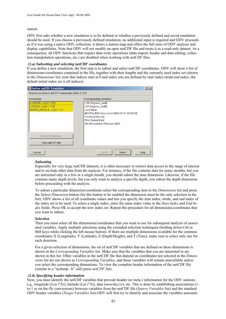
User Guide for Ocean Data View (mp) - 06.06.2002
station.
ODV first asks whether a new emulation is to be defined or whether a previously defined and saved emulation should be used. If you choose a previously defined emulation, no additional input is required and ODV proceeds as if it was using a native ODV collection: it draws a station map and offers the full suite of ODV analysis and display capabilities. Note that ODV will not modify an open netCDF file and treats it as a read-only dataset. As a consequence, all ODV functions that require data-write operations (data import, header and data editing, collec-tion manipulation operations, etc.) are disabled when working with netCDF files.
(2.a) Subsetting and selecting netCDF coordinates If you define a new emulation, the first step is to subset and select netCDF coordinates. ODV will show a list of dimensions/coordinates contained in the file, together with their lengths and the currently used index set (shown in the Dimensions list; note that indices start at 0 and index sets are defined by start index:stride:end index; the default initial index set is all indices).
Subsetting Especially for very large netCDF datasets, it is often necessary to restrict data access to the range of interest and to exclude other data from the analysis. For instance, if the file contains data for many months, but you are interested only in a few or a single month, you should subset the time dimension. Likewise, if the file contains many depth levels, but you only want to analyze a specific depth, you subset the depth dimension before proceeding with the analysis.
To subset a particular dimension/coordinate select the corresponding item in the Dimensions list and press the Subset Dimension button (for this button to be enabled the dimension must be the only selection in the list). ODV shows a list of all coordinate values and lets you specify the start index, stride, and end index of the index set to be used. To select a single index, enter the same index value in the Start Index and End In-dex fields. Press OK to accept the new index set. Repeat this procedure for all dimensions/coordinates that you want to subset.
Selection Then you must select all the dimensions/coordinates that you want to use for subsequent analysis of associ-ated variables. Apply multiple selections using the extended selection techniques (holding down Crtl or Shft keys while clicking the left mouse button). If there are multiple dimensions available for the common coordinates X (Longitude), Y (Latitude), Z (Depth/Height), and T (Time), make sure to select only one for each direction.
For a given selection of dimensions, the set of netCDF variables that are defined on these dimensions is shown in the Corresponding Variables list. Make sure that the variables that you are interested in are shown in this list. Other variables in the netCDF file that depend on coordinates not selected in the Dimen-sions list are not shown as Corresponding Variables, and those variables will remain unavailable unless you select the corresponding dimensions. To view the complete header information of the netCDF file (similar to a “ncdump –h” call) press netCDF Info.
(2.b) Specifying header information Next, you must identify the netCDF variables that provide header (or meta-) information for the ODV stations: e.g., longitude (Lon (°E)), latitude (Lat (°N)), date (mon/day/yr), etc. This is done by establishing associations (1-to-1 or on-the-fly conversions) between variables from the netCDF file (Source Variables list) and the standard ODV header variables (Target Variables list).ODV will first try to identify and associate the variables automati-
43
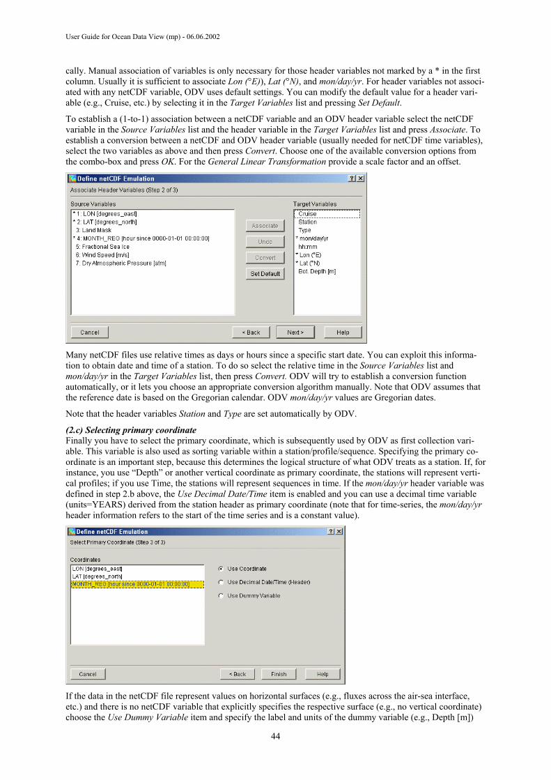
User Guide for Ocean Data View (mp) - 06.06.2002
cally. Manual association of variables is only necessary for those header variables not marked by a * in the first column. Usually it is sufficient to associate Lon (°E)), Lat (°N), and mon/day/yr. For header variables not associ-ated with any netCDF variable, ODV uses default settings. You can modify the default value for a header vari-able (e.g., Cruise, etc.) by selecting it in the Target Variables list and pressing Set Default.
To establish a (1-to-1) association between a netCDF variable and an ODV header variable select the netCDF variable in the Source Variables list and the header variable in the Target Variables list and press Associate. To establish a conversion between a netCDF and ODV header variable (usually needed for netCDF time variables), select the two variables as above and then press Convert. Choose one of the available conversion options from the combo-box and press OK. For the General Linear Transformation provide a scale factor and an offset.
Many netCDF files use relative times as days or hours since a specific start date. You can exploit this informa-tion to obtain date and time of a station. To do so select the relative time in the Source Variables list and mon/day/yr in the Target Variables list, then press Convert. ODV will try to establish a conversion function automatically, or it lets you choose an appropriate conversion algorithm manually. Note that ODV assumes that the reference date is based on the Gregorian calendar. ODV mon/day/yr values are Gregorian dates.
Note that the header variables Station and Type are set automatically by ODV.
(2.c) Selecting primary coordinate Finally you have to select the primary coordinate, which is subsequently used by ODV as first collection vari-able. This variable is also used as sorting variable within a station/profile/sequence. Specifying the primary co-ordinate is an important step, because this determines the logical structure of what ODV treats as a station. If, for instance, you use “Depth” or another vertical coordinate as primary coordinate, the stations will represent verti-cal profiles; if you use Time, the stations will represent sequences in time. If the mon/day/yr header variable was defined in step 2.b above, the Use Decimal Date/Time item is enabled and you can use a decimal time variable (units=YEARS) derived from the station header as primary coordinate (note that for time-series, the mon/day/yr header information refers to the start of the time series and is a constant value).
If the data in the netCDF file represent values on horizontal surfaces (e.g., fluxes across the air-sea interface, etc.) and there is no netCDF variable that explicitly specifies the respective surface (e.g., no vertical coordinate) choose the Use Dummy Variable item and specify the label and units of the dummy variable (e.g., Depth [m])
44

User Guide for Ocean Data View (mp) - 06.06.2002
and the associated numerical value that defines the surface (e.g., 0 for ocean surface).
(3) Exploring the netCDF file
After completing steps 2.a through 2.c ODV has sufficient information to access the netCDF data in the user requested way. ODV will draw a station map and then offers the full suite of ODV analysis and display capabili-ties. Note that ODV will not modify an open netCDF file and treats it as a read-only dataset. As a consequence, all ODV functions that require data-write operations (data import, header and data editing, collection manipula-tion operations, etc.) are disabled when working with netCDF files.
Also note that data access from netCDF files is slower as compared with native ODV collections. If you are using large netCDF datasets with tens of thousands of (emulated) stations and you are experiencing slow buildup of SCATTER or SURFACE plots, you should consider subsetting (see above) or you should export the netCDF data to a native ODV collection using Export>ODV Collection and then use the newly created collection for analysis and visualization.
In order to produce vertical sections you should switch to SECTION mode, for instance, by choosing Configura-tion>UseTemplate>SECTION 2 Win and then define sections of your choice using Define Section>Define Sec-tion Spine from the map popup menu. To create property distributions on horizontal surfaces or other longi-tude/latitude iso-surfaces switch to SURFACE mode, for instance, by choosing Configura-tion>UseTemplate>SURFACE 1 Win. Then define iso-surface variables through Configuration>Iso-Surface Variables and use them as Z-variables on the plot windows.
Note that when working with netCDF files the nc-emulation settings as defined during steps 2.a to 2.c is saved on disk when you save your current configuration. Saved nc-emulation settings can be re-used later, thereby avoiding unnecessary re-definitions.
45

User Guide for Ocean Data View (mp) - 06.06.2002
13 Manipulating Collections
13.1 Changing the Set of Collection Variables In situations when new data become available for variables that are not already included in a given data collec-tion, you might want to add these variables to the collection. Also, sometimes you might want to delete some of the existing variables from a collection.
To add and/or delete collection variables open the collection and choose Collection>Add/Delete Vari-ables from the main menu. Add a new variable by entering the variable label (including units enclosed by brackets [ ]) in the “New Variable” control and press Add. You delete a variable by selecting it in the “De-fined Variables” list and pressing Delete. You can change the order of the variables by choosing one and moving it Up or Down. Press OK when you are done. Note that the entire collection has to be re-written which might take some time for large data collections.
13.2 Sorting and Condensing The station search and selection algorithms of ODV work most efficiently if the stations in a collection are or-dered in a specific way. Therefore, it is recommend that you sort and condense your collections after importing, replacing, merging or deleting large numbers of stations. You invoke the sort and condense procedure by choos-ing Collection>Sort and Condense from ODV’s main menu.
13.3 Deleting Selected Station-Subset You can delete the currently selected stations from the collection by choosing Collection>Delete Station Subset from ODV’s main menu. To delete the current station only, choose Collection >Delete Current Station. Note that the data-space of the deleted stations in the collection disk files is not freed until you sort and condense the collection.
46

User Guide for Ocean Data View (mp) - 06.06.2002
14 Utilities
14.1 Data Inventory Tables You can produce an inventory table of the currently open collection by choosing Utilities>Inventory Table from ODV’s main menu. The output file is plain ASCII and is written to the collection directory (extension .inv).
14.2 Temporal Data Distribution Plots You can produce plots of the temporal distribution of the currently selected stations (by months and years) by choosing Utilities>Temporal Distribution from ODV’s main menu.
14.3 Data Retrieval ODV can calculate and export average values and standard deviations for selected variables using all original data points within given boxes defined by Lon/Lat/Depth intervals. Note that for the retrieval only those stations are used that satisfy the current selection criteria and are show in the map. You can obtain averages for different years, months, seasons etc. by applying appropriate station selection criteria prior to invoking the retrieval. To select the data retrieval option choose Utilities>Data Retrieval from ODV’s main menu. ODV will prompt you for a retrieval input file (extension .rtv) containing geometry information for the boxes and the variable numbers for which output is to be produced. The .rtv file has to be prepared prior to invoking the retrieval option.
The format of the .rtv file is as follows:
• plain ASCII, one box/variable definition per line, 7 numbers separated by (one or more) spaces,
• meaning of numbers: lon lat dep (box center) dlon dlat ddep variable#.
Once you have specified a .rtv file, ODV will start working. Note that while averaging, ODV will check for data outliers and will use only data within 3 standard deviations of the mean. The output will be written to a file with
47
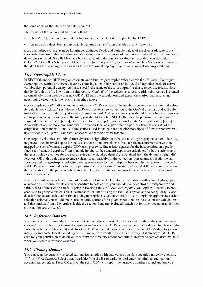
User Guide for Ocean Data View (mp) - 06.06.2002
the same name as the .rtv file and extension .out.
The format of the .out output file is as follows:
• plain ASCII, one line of output per line in the .rtv file, 11 values separated by TABS,
• meaning of values: lon lat dep variable# (same as in .rtv) alon alat adep aval +- sdev nu nr.
alon, alat, adep, aval are average Longitude, Latitude, Depth and variable values of the data used, sdev is the standard-deviation of the individual variable values, nu is the number of data points used and nr is the number of data points rejected. Note that for each box retrieval all individual data values are exported to ASCII files ODVrtv?.dat in ODV’s temporary files directory (normally: c:\Program Files\Ocean Data View (mp)\Temp). In the .dat files the meaning of values is as follows: # lon lat dep day-of-year value weight used/rejected-flag.
14.4 Geostrophic Flows In SECTION mode, ODV lets you calculate and visualize geostrophic velocities via the Utilities>Geostrophic Flows option. Define a reference layer by choosing a depth horizon or an iso-level of any other basic or derived variable (i.e., potential density, etc.) and specify the name of the .o4x output file that receives the results. Note that by default this file is written to subdirectory ‘GeoVel’ of the collection directory (this subdirectory is created automatically if not already present). ODV will start the calculations and export the station-pair results and geostrophic velocities to the .o4x file specified above.
Once completed, ODV allows you to invoke a new ODV session on the newly calculated section pair and veloc-ity data. If you click on ‘Yes’, the new ODV will create a new collection in the GeoVel directory and will auto-matically import the .o4x file just written. Using standard ODV procedures, you should then define an appropri-ate map domain by zooming into the map, you should switch to SECTION mode by pressing F11, and you should define Geostr. Vel. [cm/s], Geostr. Vel. (north comp.) [cm/s] and/or Geostr. Vel. (east comp.) [cm/s] as Z-variable of one or more plot windows. The station label of a given station-pair A->B:alpha consists of the original station numbers A and B of the stations used in the pair and the direction alpha of flow for positive val-ues of Geostr. Vel. [cm/s] (alpha=0: eastward; alpha=90: northward; etc.).
Geostrophic velocities are derived from dynamic height differences between two hydrographic stations. Because, in general, the observed depths for the two stations do not match, in a first step the measurements have to be mapped to a set of common depths (ODV uses piecewise linear least squares for the interpolation on a prede-fined set of standard depths). Then dynamic heights at the standard depths are calculated for both stations, and the geostrophic velocities for the station pair (at the standard depths) are obtained from the dynamic height dif-ferences. ODV also calculates average values for all variables in the collection (pair-averages). Both, the pair-averages and the geostrophic velocities are representative for the mid-point between the two stations involved, and ODV writes those values to the output .o4x file for a “virtual” pair station located at the mid-point between the two stations in the pair (note the station label of the pair station contains the station labels of the original stations involved).
Note that geostrophic velocities are not calculated close to the Equator or for stations with sparse hydrographic observations. Because results are very sensitive to data errors, you should quality control the temperature and salinity data of the section carefully prior to invoking the Utilities>Geostrophic Flows option. One way to pro-ceed is to flag suspicious data as ”Questionable” or ”Bad” using the Edit Data option and to accept only ”Good” data for display and calculation (by applying appropriate selection criteria). Also by applying appropriate station selection criteria, you should make sure that only stations for a given expedition are included in the calculations and that stations from other cruises inside the section-band are excluded (watch out for other oceanographic lines crossing the section-band).
14.5 Reference Datasets You can save the original data of the current plot windows in ASCII disk files and use these data later as refer-ence datasets by choosing Utilities>Define as Reference from ODV’s main menu. Enter a descriptive text identi-fying the reference data (txtID) and click OK. ODV will create a sub-directory in the local ODV directory (nor-mally <home>\odv_local) named reference\txtID and writes all files to this directory. If it already exists, ODV asks for your permission to delete all files from the directory before continuing. Reference data are used by ODV when you define difference variables.
14.6 Finding Outliers You can scan the currently selected stations for samples with data values outside a specified range by choosing Utilities>Find Outliers. Select a scan-variable from the list of variables and enter the minimal and maximal accepted range values. Press OK to start the scan. ODV will report the number of outliers found and lets you
48

User Guide for Ocean Data View (mp) - 06.06.2002
view the list of outliers and lets you inspect and modify the outlier data values or quality flags.
If you check Inspect and Edit Outliers, ODV will visit all identified outliers and allows you to delete the respec-tive value or to mark it as “Questionable” or “Bad”. If you press Aplly to All, ODV applies the selected to all outliers, otherwise the user is prompted for an action for each individual outlier. Note that the respective outlier is marked in the data plots.
14.7 Finding Redundant Stations You can scan a collection for stations with identical or nearly identical positions and times of occupation (redun-dant stations) by choosing Utilities>Find Redundant Stations. The list of redundant stations is written to disk (default name redundant.lst). In the redundant.lst file, blank lines separate sets of redundant stations. For each station the following information is given: (1) internal no., (2) cruise label, (3) station label, (4) station type, (5) date, (6) longitude, (7) latitude, (8) no. of observed levels, (9) deepest level, (10) availability indicators for basic variables 2...nvar (e.g., 7 means that between 70 and 79% of the observed levels contain data for a given vari-able).To delete a redundant station, make it the current station using Select Station by Name from the map popup menu and then delete it using Actions>Delete Current Station.
Note that for large collections, the redundant stations scan is a lengthy procedure.
49
User Guide for Ocean Data View (mp) - 06.06.2002
15 Graphics Objects You can improve ODV graphics output and give it a finishing, professional touch by adding text, highlighting data points and adding lines or other geometric objects. ODV graphics objects include (1) text annotations, (2) straight lines, (3) rectangles and squares, (4) ellipses and circles, (5) polylines (straight-line segments or Bezier smoothed), (6) filled polygons (straight-line segments or Bezier smoothed), (7) symbols, (8) symbol sets and (9) legends.
Creation Except for legends, which are created automatically, you create and add any other graphics object by choosing Extras>Add Graphics Object>... (where ”...” represents the desired object type) from the map or data plot popup menus or by choosing Add Graphics Object>... from the background popup menu. After creation, dialog boxes are presented that let you define various properties of the object. These properties can be changed (see ”Edit” below) at any time. A graphics object is owned by the window (or background area) from which the creation was initiated, and the coordinates of the graphics object are recorded in the respective window coordinate system. As a consequence, all objects of a window follow automatically when the respective window is moved or resized.
Edit and Delete The properties of a given object can be modified by moving the mouse over it (for symbol sets move the mouse over one of the symbols), clicking the right mouse button and choosing Edit Object from the popup menu. Dia-log boxes (different for the different objects) appear and let you change properties easily and quickly. Any graphics object may be clipped to its parent window (check the ”clip to window” box), and you may request that it is drawn before the data of the window are drawn (check the ”pre-data plot” box).You delete an object by moving the mouse over it, clicking the right mouse button and choosing Delete Object.
Dragging If the attribute ”allow dragging” of a graphics object is set, the object can be re-positioned by simply dragging it to a different location. To drag an object, move the mouse over it, click and hold down the left mouse button and move the mouse. By default, dragging is switched on initially for all graphics objects except symbol sets which are linked to data values. You can change the ” allow dragging” attribute at any time using the Edit dialogs (see above).
15.1 Annotations You can add annotations to the ODV graphics window by choosing (Extras>)Add Graphics Object>Annotation from the background, map or data plot popup menus. A cross-hair cursor will appear, and you should move it to the location where the annotation should appear and then click the left mouse button. Note that the window from which the creation was initiated owns the respective object. When adding (or editing) annotations you may set the position, orientation (degrees, counter-clockwise), font size (pt), color and alignment parameter of the anno-tation text. Annotations can have a frame, and the annotation rectangle can be filled before drawing the annota-tion. You can choose different colors for all these items. Maximum length of the annotation text is 255 charac-ters. For special text effects, you can use the following control sequences within the text:
~$ switch to Symbol font (Greek symbols) ~# switch to normal text font ~~ produce ˜ character ~s produce ß character ~" next character as Umlaut' ~^ next character as superscript ~_ next character as subscript.
Like all other graphics objects, you can drag an annotation to a different position by moving the mouse cursor over it, pressing and holding down the left mouse button and moving the mouse. You can edit an annotation by moving the mouse over it, clicking the right mouse button and choosing Edit Object from the popup menu. To delete an annotation (all annotations) choose Delete Object (Delete All Objects) from its popup menu.
Note that the axis labels of the data plot windows are implemented as (automatic) annotations. They are created automatically when the plot window is drawn and they are deleted when the respective data plot window is de-leted. You can drag, edit or delete axis labels, but please note that the automatic versions re-appear if the plot window is redrawn. If you want to change an axis label ”permanently” you should create an annotation manually by choosing Extras>Add Graphics Object>Annotation from the background popup menu. Make sure that you save the configuration after defining the new annotation and delete the automatic axis annotation before printing or writing PostScript files.
50
User Guide for Ocean Data View (mp) - 06.06.2002
15.2 Lines and Polygons You add straight lines, polylines and polygons to the map, data plots or background by choosing (Extras>)Add Graphics Object>Line, ...>Polyline or ...>Polygon from the map, data plot or background popup menus. In all three cases the cursor changes to a cross hair and you should proceed by specifying the nodes of the object. For a ”Line” you must define starting- and endpoint: move the cross-hair to the start of the line and click the left mouse button, then move to the end-point and click the left button again. For Polyline or Polygon you may de-fine up 1000 points. Note that polygons are closed automatically by ODV. If you want to delete a point, move the cross hair close to it and click the right mouse button. You end the definition of polygon or polyline points by pressing ENTER.
Once you have specified the nodes of the line, polyline or polygon, ODV presents a dialog box that lets you define color, width and type of the (poly)line and the fill-color of the polygon (ignored for Line and Polyline; choose ”none” as fill-color to avoid filling of the polygon). Also note that lines wider than 1 pixel are always solid on many screen and printer devices. However, the requested line-type is always honored in ODV Post-Script files. Polylines and polygons may be smoothed by checking the ”Bezier smoothing” box.
15.3 Rectangles and Ellipses You add rectangles (squares) and ellipses (circles) to the map, data plots or background by choosing (Ex-tras>)Add Graphics Object>Rectangle, or ...>Ellipse from the map, data plot or background popup menus. A red zoom rectangle will appear that represents the bounding box of the new rectangle or ellipse. The zoom rec-tangle can be moved and resized, press ENTER to accept a setting. A dialog box appears that lets you define properties of the rectangle or ellipse (for details see Lines and Polygons).
15.4 Symbols You add symbols (dots, squares, diamonds, triangles, inverted triangles, stars, crosses, pluses) to the map, data plots or background by choosing (Extras>)Add Graphics Object>Symbol from the map, data plot or background popup menus. A cross-hair cursor will appear, and you should move it to the location where the symbol should appear. Then click the left mouse button. The “Symbol Properties” dialog box appears and lets you set various symbol properties.
15.5 Symbol Sets and Legends You can highlight a subset of the data points in a plot window or a subset of stations in the map by assigning a symbol to the selected data points (symbol-set). To create a symbol-set for a data window or the map, move the mouse over this window and choose Extras>Add Graphics Object>Symbol Set. The symbol set selection dialog box appears and lets you select the subset of data points (specify cruise labels, stations and/or individual sam-ples). Press the << button to add the points to the list of selections. Press OK once all desired points are selected. Then the symbol set properties dialog box appears which lets you define the symbol characteristics. A symbol set can have a descriptive text (legend), which will automatically be added to the legends of the respective win-dow (check the add to legends box). Unlike other graphics objects, symbol sets cannot be dragged because they are associated with the selected data points. You can change all properties of a symbol set at any time by moving the mouse over any one of its symbols, clicking the right mouse button and choosing Edit Graphics Object.
If a data window or the map contain symbol sets with the add to legends option switched on, a legend box con-taining the symbol and legend text of all symbol sets for this window appears. Legend sets can be dragged to different locations and their properties (the size of the legend box is modified by changing the font size for the legend text) can be modified at any time (move mouse over legend set, click right mouse button and choose Edit Graphics Object).
51
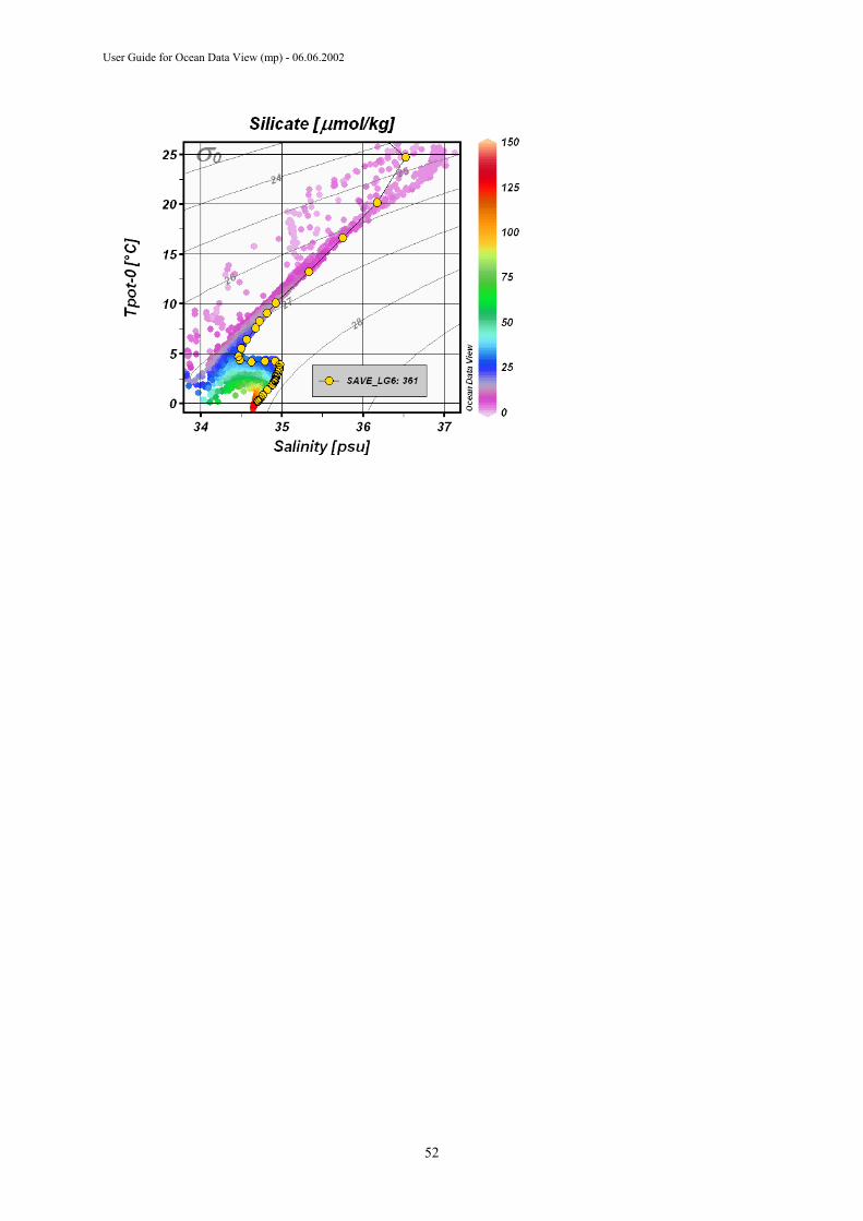
User Guide for Ocean Data View (mp) - 06.06.2002
52
User Guide for Ocean Data View (mp) - 06.06.2002
16 More …
16.1 Gazetteer of Undersea Features ODV can be used to identify undersea features like seamounts, ridges, fracture zones, troughs, basins, etc. To invoke the gazetteer option, choose Extras>Gazetteer from the map popup menu (or press Ctrl-g while the mouse is over the map). The gazetteer dialog box is shown and lets you select a specific database, lets you spec-ify feature selection criteria as well as size and color of the gazetteer marks drawn by ODV. When you press OK, the information from the selected gazetteer database is loaded, and the feature positions are marked in the map. Moving the mouse close to a feature point invokes a popup window displaying the name of the feature. To switch off the gazetteer marks, invoke the gazetteer dialog box again and choose none in the Database list.
Three gazetteer files are provided with the ODV distribution: (1) GazetteerGEBCO.gzt from the Int. Hydrogr. Bureau (IHB), (2) GazetteerBGN.gzt from the US Defense Mapping Agency, and (3) WHP_Sections.gzt, which is a compilation of the sections occupied during the WOCE Hydrographic Programme. You can produce feature subsets by specifying a feature type and/or feature name sub-string using the gazetteer dialog box. Note that the name and type selections are case-insensitive. Use the gazetteer feature selection if you know the name of a feature (or part of the name) and want to identify its location (note that you might have to open the map to global extent in order to see the feature mark). Gazetteer settings are not saved in configuration files. Whenever you open a collection, the gazetteer option is switched off initially and you have to switch it on in order to use it.
Gazetteer files can be edited and extended. You can also create your own, new gazetteer databases. In order to use a private gazetteer with ODV, the file must have the extension .gzt, it must be located in the ODV gazetteer directory (normally: c:\Program Files\Ocean Data View (mp)\include\gazetteers) and its format must satisfy the specifications below:
The first line of the file must start with % GZT01: followed by the name of the file.
Then there are 7 lines starting with % and containing arbitrary comments.
The next line must be: Feature;Type;No;East-Longitude;North-Latitude; there has to be one blank line fol-lowing.
The rest of the file contains the actual item definitions. Each feature is listed on a separate line.
The name of the feature, its type, the number of lon/lat points and the longitude/latitude entries are separated by semicolons ”;”. Longitude is specified in degrees East (0-360). The number of lon/lat points can be up to 1500, and the length of a line may be up to 200,000 characters.
16.2 Drag-and-Drop WIN32:
You can drag and drop files on the ODV window or icon. Depending on the extension of the dropped file, ODV will perform the following actions:
.var: close current collection and open dropped one. .o4x: import data from dropped file into currently open collection (if no collection is open when the file is
dropped, ODV creates a new collection in the directory of the dropped file and imports the data into the newly created collection).
.txt: import data from dropped file (assuming generic ODV SpreadSheet text file) into currently open collec-
tion (if no collection is open when the file is dropped, ODV creates a new collection in the directory of the dropped file and imports the data into the newly created collection).
UNIX:
Drag-and-drop is currently not implemented under UNIX. However, by using appropriate file names as com-mand line arguments, you can obtain similar results. Start ODV from any Terminal window by typing: odv [file name[.extension]]. Note that for file name you either use absolute pathnames or pathnames relative to the direc-tory from which you start ODV. If you use a relative pathname, “.” and “..” are not allowed. You can use com-mand line arguments to …
1. … start ODV and open an existing collection: use the collection name for file name. If you omit an extension, the default .var is used.
2. … create a new collection and import data: use the name of the data file (must be one of ODV’s im-
53
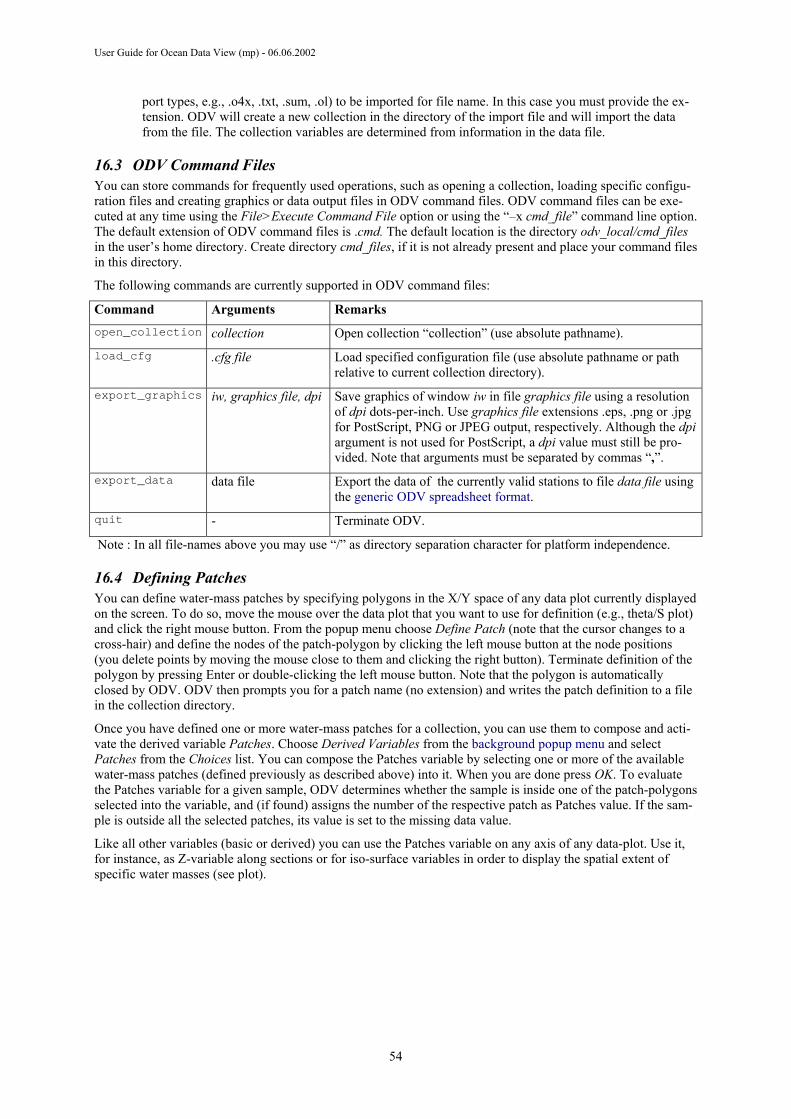
User Guide for Ocean Data View (mp) - 06.06.2002
port types, e.g., .o4x, .txt, .sum, .ol) to be imported for file name. In this case you must provide the ex-tension. ODV will create a new collection in the directory of the import file and will import the data from the file. The collection variables are determined from information in the data file.
16.3 ODV Command Files You can store commands for frequently used operations, such as opening a collection, loading specific configu-ration files and creating graphics or data output files in ODV command files. ODV command files can be exe-cuted at any time using the File>Execute Command File option or using the “–x cmd_file” command line option. The default extension of ODV command files is .cmd. The default location is the directory odv_local/cmd_files in the user’s home directory. Create directory cmd_files, if it is not already present and place your command files in this directory.
The following commands are currently supported in ODV command files:
Command Arguments Remarks open_collection collection Open collection “collection” (use absolute pathname).
load_cfg .cfg file Load specified configuration file (use absolute pathname or path relative to current collection directory).
export_graphics iw, graphics file, dpi Save graphics of window iw in file graphics file using a resolution of dpi dots-per-inch. Use graphics file extensions .eps, .png or .jpg for PostScript, PNG or JPEG output, respectively. Although the dpi argument is not used for PostScript, a dpi value must still be pro-vided. Note that arguments must be separated by commas “,”.
export_data data file Export the data of the currently valid stations to file data file using the generic ODV spreadsheet format.
quit - Terminate ODV.
Note : In all file-names above you may use “/” as directory separation character for platform independence.
16.4 Defining Patches You can define water-mass patches by specifying polygons in the X/Y space of any data plot currently displayed on the screen. To do so, move the mouse over the data plot that you want to use for definition (e.g., theta/S plot) and click the right mouse button. From the popup menu choose Define Patch (note that the cursor changes to a cross-hair) and define the nodes of the patch-polygon by clicking the left mouse button at the node positions (you delete points by moving the mouse close to them and clicking the right button). Terminate definition of the polygon by pressing Enter or double-clicking the left mouse button. Note that the polygon is automatically closed by ODV. ODV then prompts you for a patch name (no extension) and writes the patch definition to a file in the collection directory.
Once you have defined one or more water-mass patches for a collection, you can use them to compose and acti-vate the derived variable Patches. Choose Derived Variables from the background popup menu and select Patches from the Choices list. You can compose the Patches variable by selecting one or more of the available water-mass patches (defined previously as described above) into it. When you are done press OK. To evaluate the Patches variable for a given sample, ODV determines whether the sample is inside one of the patch-polygons selected into the variable, and (if found) assigns the number of the respective patch as Patches value. If the sam-ple is outside all the selected patches, its value is set to the missing data value.
Like all other variables (basic or derived) you can use the Patches variable on any axis of any data-plot. Use it, for instance, as Z-variable along sections or for iso-surface variables in order to display the spatial extent of specific water masses (see plot).
54
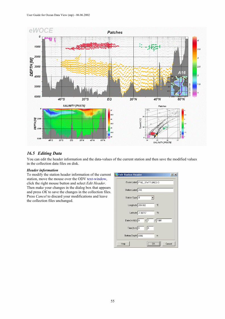
User Guide for Ocean Data View (mp) - 06.06.2002
16.5 Editing Data You can edit the header information and the data-values of the current station and then save the modified values in the collection data files on disk.
Header information To modify the station header information of the current station, move the mouse over the ODV text-window, click the right mouse button and select Edit Header. Then make your changes in the dialog box that appears and press OK to save the changes in the collection files. Press Cancel to discard your modifications and leave the collection files unchanged.
55
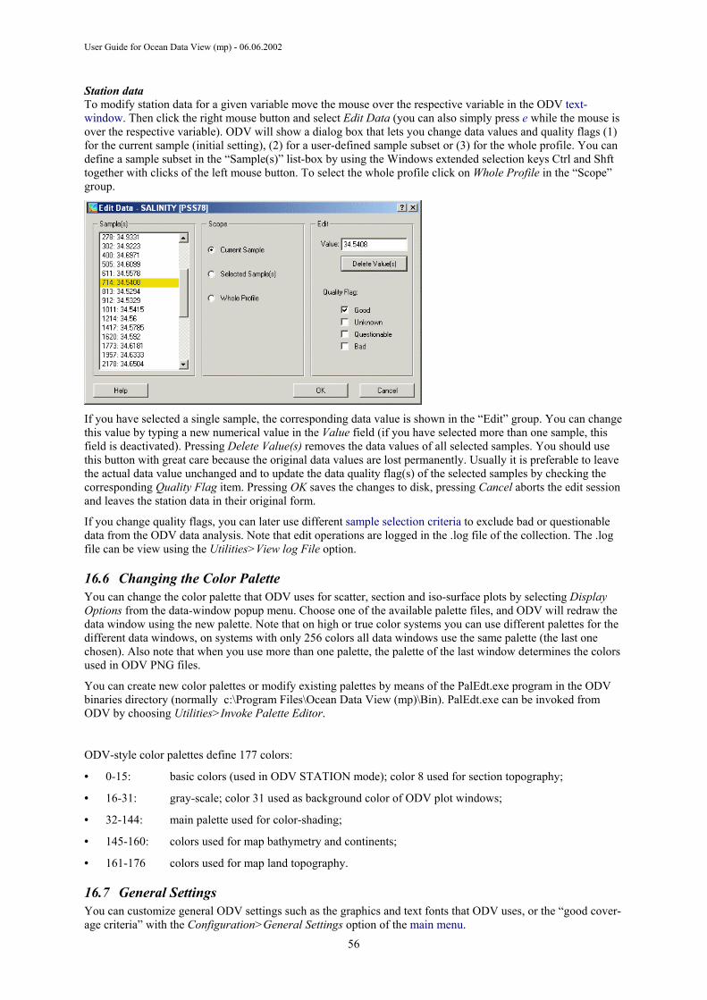
User Guide for Ocean Data View (mp) - 06.06.2002
Station data To modify station data for a given variable move the mouse over the respective variable in the ODV text-window. Then click the right mouse button and select Edit Data (you can also simply press e while the mouse is over the respective variable). ODV will show a dialog box that lets you change data values and quality flags (1) for the current sample (initial setting), (2) for a user-defined sample subset or (3) for the whole profile. You can define a sample subset in the “Sample(s)” list-box by using the Windows extended selection keys Ctrl and Shft together with clicks of the left mouse button. To select the whole profile click on Whole Profile in the “Scope” group.
If you have selected a single sample, the corresponding data value is shown in the “Edit” group. You can change this value by typing a new numerical value in the Value field (if you have selected more than one sample, this field is deactivated). Pressing Delete Value(s) removes the data values of all selected samples. You should use this button with great care because the original data values are lost permanently. Usually it is preferable to leave the actual data value unchanged and to update the data quality flag(s) of the selected samples by checking the corresponding Quality Flag item. Pressing OK saves the changes to disk, pressing Cancel aborts the edit session and leaves the station data in their original form.
If you change quality flags, you can later use different sample selection criteria to exclude bad or questionable data from the ODV data analysis. Note that edit operations are logged in the .log file of the collection. The .log file can be view using the Utilities>View log File option.
16.6 Changing the Color Palette You can change the color palette that ODV uses for scatter, section and iso-surface plots by selecting Display Options from the data-window popup menu. Choose one of the available palette files, and ODV will redraw the data window using the new palette. Note that on high or true color systems you can use different palettes for the different data windows, on systems with only 256 colors all data windows use the same palette (the last one chosen). Also note that when you use more than one palette, the palette of the last window determines the colors used in ODV PNG files.
You can create new color palettes or modify existing palettes by means of the PalEdt.exe program in the ODV binaries directory (normally c:\Program Files\Ocean Data View (mp)\Bin). PalEdt.exe can be invoked from ODV by choosing Utilities>Invoke Palette Editor.
ODV-style color palettes define 177 colors:
• 0-15: basic colors (used in ODV STATION mode); color 8 used for section topography;
• 16-31: gray-scale; color 31 used as background color of ODV plot windows;
• 32-144: main palette used for color-shading;
• 145-160: colors used for map bathymetry and continents;
• 161-176 colors used for map land topography.
16.7 General Settings You can customize general ODV settings such as the graphics and text fonts that ODV uses, or the “good cover-age criteria” with the Configuration>General Settings option of the main menu. 56
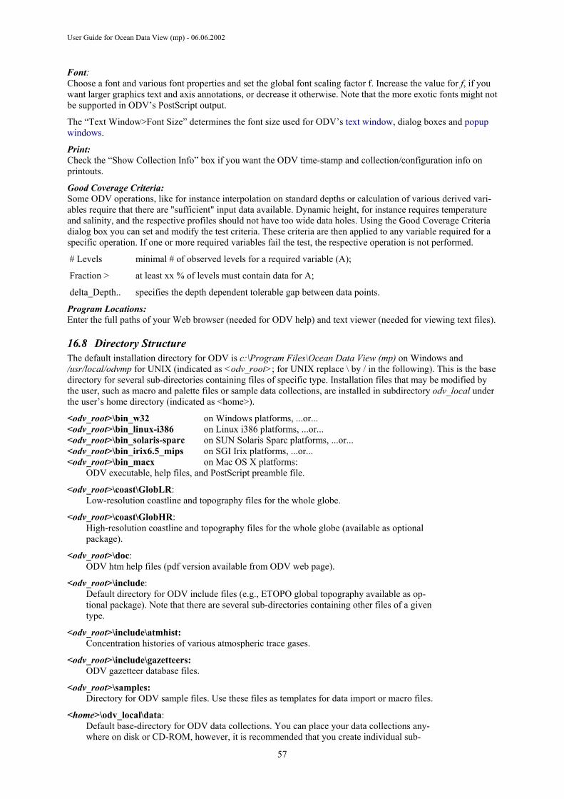
User Guide for Ocean Data View (mp) - 06.06.2002
Font: Choose a font and various font properties and set the global font scaling factor f. Increase the value for f, if you want larger graphics text and axis annotations, or decrease it otherwise. Note that the more exotic fonts might not be supported in ODV’s PostScript output.
The “Text Window>Font Size” determines the font size used for ODV’s text window, dialog boxes and popup windows.
Print: Check the “Show Collection Info” box if you want the ODV time-stamp and collection/configuration info on printouts.
Good Coverage Criteria: Some ODV operations, like for instance interpolation on standard depths or calculation of various derived vari-ables require that there are "sufficient" input data available. Dynamic height, for instance requires temperature and salinity, and the respective profiles should not have too wide data holes. Using the Good Coverage Criteria dialog box you can set and modify the test criteria. These criteria are then applied to any variable required for a specific operation. If one or more required variables fail the test, the respective operation is not performed.
# Levels minimal # of observed levels for a required variable (A);
Fraction > at least xx % of levels must contain data for A;
delta_Depth.. specifies the depth dependent tolerable gap between data points.
Program Locations: Enter the full paths of your Web browser (needed for ODV help) and text viewer (needed for viewing text files).
16.8 Directory Structure The default installation directory for ODV is c:\Program Files\Ocean Data View (mp) on Windows and /usr/local/odvmp for UNIX (indicated as <odv_root>; for UNIX replace \ by / in the following). This is the base directory for several sub-directories containing files of specific type. Installation files that may be modified by the user, such as macro and palette files or sample data collections, are installed in subdirectory odv_local under the user’s home directory (indicated as <home>).
<odv_root>\bin_w32 on Windows platforms, ...or... <odv_root>\bin_linux-i386 on Linux i386 platforms, ...or... <odv_root>\bin_solaris-sparc on SUN Solaris Sparc platforms, ...or... <odv_root>\bin_irix6.5_mips on SGI Irix platforms, ...or... <odv_root>\bin_macx on Mac OS X platforms:
ODV executable, help files, and PostScript preamble file.
<odv_root>\coast\GlobLR: Low-resolution coastline and topography files for the whole globe.
<odv_root>\coast\GlobHR: High-resolution coastline and topography files for the whole globe (available as optional package).
<odv_root>\doc: ODV htm help files (pdf version available from ODV web page).
<odv_root>\include: Default directory for ODV include files (e.g., ETOPO global topography available as op-tional package). Note that there are several sub-directories containing other files of a given type.
<odv_root>\include\atmhist: Concentration histories of various atmospheric trace gases.
<odv_root>\include\gazetteers: ODV gazetteer database files.
<odv_root>\samples: Directory for ODV sample files. Use these files as templates for data import or macro files.
<home>\odv_local\data: Default base-directory for ODV data collections. You can place your data collections any-where on disk or CD-ROM, however, it is recommended that you create individual sub-
57

User Guide for Ocean Data View (mp) - 06.06.2002
directories for every collection that you maintain.
<home>\odv_local\data\SAVE: Sample ODV data collection containing the South Atlantic Ventilation Experiment data.
<home>\odv_local\include\macros: ODV macro files (.mac).
<home>\odv_local\include\palettes: ODV palette files (.pal).
User’s default Temp directory: Directory for temporary files. ODV routinely removes files with names starting with ODV from this directory if they are older than 3 days.
16.9 Hardware Requirements The multi-platform version of ODV runs on computers with the Windows (9x/Me/NT/2000/XP), Linux, various UNIX, or Mac OS X operating systems. The hardcopy routines of ODV have been tested on black white and color Apple LaserWriter, Canon Laser Copier and HP DeskJet printers, but should work on other printers as well. If you have a PostScript printer available, you can use ODV’s Save As PostScript option instead of Print, for faster and higher quality output. Also consider to write screen graphics to high-resolution .png or .jpg files. Note that administrator privileges are required for installation of ODV(mp) on some systems.
16.10 Limitations No. of stations per collection No limit
No. of data values per station 100,000
No. of levels per station 20,000
No. of data plot windows 20
No. of variables stored in a collection 50
No. of contour lines per window 50
Length of collection names (characters) 30
Length of variable names (characters) 60
Length of cruise labels (characters) 20
Length of station labels (characters) 20
58
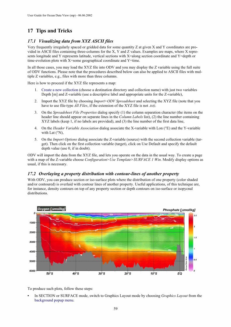
User Guide for Ocean Data View (mp) - 06.06.2002
17 Tips and Tricks
17.1 Visualizing data from XYZ ASCII files Very frequently irregularly spaced or gridded data for some quantity Z at given X and Y coordinates are pro-vided in ASCII files containing three-columns for the X, Y and Z values. Examples are maps, where X repre-sents longitude and Y represents latitude, vertical sections with X=along section coordinate and Y=depth or time-evolution plots with X=some geographical coordinate and Y=time.
In all those cases, you may load the XYZ file into ODV and you may display the Z variable using the full suite of ODV functions. Please note that the procedures described below can also be applied to ASCII files with mul-tiple Z variables, e.g., files with more than three columns.
Here is how to proceed if the XYZ file represents a map:
1. Create a new collection (choose a destination directory and collection name) with just two variables Depth [m] and Z-variable (use a descriptive label and appropriate units for the Z-variable),
2. Import the XYZ file by choosing Import>ODV Spreadsheet and selecting the XYZ file (note that you have to use file-type All Files, if the extension of the XYZ file is not .txt).
3. On the Spreadsheet File Properties dialog specify (1) the column separation character (the items on the header line should appear on separate lines in the Column Labels list), (2) the line number containing XYZ labels (keep 1, if no labels are provided), and (3) the line number of the first data line,
4. On the Header Variable Association dialog associate the X-variable with Lon (°E) and the Y-variable with Lat (°N),
5. On the Import Options dialog associate the Z-variable (source) with the second collection variable (tar-get). Then click on the first collection variable (target), click on Use Default and specify the default depth value (use 0, if in doubt).
ODV will import the data from the XYZ file, and lets you operate on the data in the usual way. To create a page with a map of the Z-variable choose Configuration>Use Template>SURFACE 1 Win. Modify display options as usual, if this is necessary.
17.2 Overlaying a property distribution with contour-lines of another property With ODV, you can produce section or iso-surface plots where the distribution of one property (color shaded and/or contoured) is overlaid with contour lines of another property. Useful applications, of this technique are, for instance, density contours on top of any property section or depth contours on iso-surface or isopycnal distributions.
To produce such plots, follow these steps:
• In SECTION or SURFACE mode, switch to Graphics Layout mode by choosing Graphics Layout from the background popup menu.
59
User Guide for Ocean Data View (mp) - 06.06.2002
• Setup the window for the underlying distribution (window a: define size and position; select a Z-variable for that window (property A)).
• Create a twin of window a by moving the mouse over window a, clicking the right mouse button and select-ing Create Twin. Move the mouse over the newly created window (window b), click the right mouse button and select Move/Resize. Move (without changing the size) window b over window a until they coincide. Press ENTER to accept. Now select the Z-variable for the overlay contour lines in window b (property B). Leave the Graphics Layout mode by pressing ENTER.
• When ODV has redrawn the data plots, move the mouse over window b, right-click the mouse and select Display Options. Check the VG Gridding button, as background color choose none (first choice), and click on the Properties button. Uncheck the Do Color Shading mark and proceed by defining contour lines . Use a color for the contour lines that will be clearly visible on top of the color distribution of property A (e.g., white or black). Click OK to accept the display option settings.
• When ODV has redrawn the data plots, move the mouse over the background area and press r to enforce a redraw of all data windows. Before printing or PostScript, PNG or JPG export, separate the labels of proper-ties A and B by dragging the respective annotations (move the mouse over the a label, hold down the left mouse button and move; note that this separation has to be repeated after redrawing).
• If you are satisfied, save the configuration as usual for later use.
Note that for a window entirely overlain by another window (like window a), the only way to access and modify its properties is via the Configuration>Window Properties option from the main menu.
17.3 Using ODV Graphics in Publications and on Web Pages ODV graphics, either as entire ODV pages or individual data plots, can be included in print documents, posters or on Web pages.
For Web pages you should create PNG or JPG files of the whole ODV screen or of individual plots (press Ctrl-s while the mouse is over the background or the respective plot window and choose PNG or JPG as output type). Note that you can set the resolution of the graphics file (default: screen resolution). Then use the PNG or JPG graphics files in your web pages or in text documents.
For print documents you can either produce PNG files with a high resolution, or you can use ODV PostScript (.eps) output instead.
A variety of typesetting and page design software supports the import of Encapsulated PostScript files (.eps) in mixed text/graphics pages (e.g., MS Word or compatibles, LaTeX, Adobe PageMaker, etc.). If you use the La-Tex typesetting system, see the file Pssample.tex (usually in directory c:\Program Files\Ocean Data View (mp)\Samples) for an example on how to include PostScript graphics in TeX documents. Note that the required epsf and epsfig style files are also included in the samples directory.
If you use Word or PageMaker or other publishing software follow these guidelines: Compose your page as usual and insert the respective ODV PostScript file at the right position. Adjust the size of the figure appropri-ately. When you are done composing the page you can directly print the document on a PostScript printer. If no PostScript printer is available you need to have a PostScript printer-driver and the GhostScript/GhostView pack-age (http://www.cs.wisc.edu/~ghost/aladdin/index.html) installed on your machine. In that case select the Post-Script printer-driver as printer and redirect the output into a file. Open this file with GhostView and print to any printer connected to your system.
17.4 Preparing Coastline and Bathymetry Files ODV comes with a coarse resolution global set of coastline and bathymetry files (GlobLR). Higher resolution versions of coast/bathymetry data are available for the whole globe (GlobHR) or for selected regions as optional packages (Baltic, BayOfBiscay, MedHR, and MeditHR). If you need high-resolution representations of coastline and bathymetry for a region not provided by the ODV distribution and if you have such high-resolution data available, here is how to produce ODV usable files.
Preparing New Files The data for the coastline and bathymetry contours must be in separate files. I recommend to use ”World” as the name for the coastline file. For naming of the bathymetry files you must use the ”xxxm” scheme, where xxx represents the depth of the respective depth contour (no white space between the depth value and the ”m”). For the ASCII version of the coast/bathymetry files the file extension must be .coa.
The lat/lon coordinates of the coast (or a depth contour) are stored in individual polygon segments with less than 1500 vertices each. Note that lat and lon are decimal, lon is in degrees East (0 – 360) and lat is in degrees North 60

User Guide for Ocean Data View (mp) - 06.06.2002
(-90 – 90). The format of a polygon segment in a .coa file is as follows:
nT nS
lat_1 lon_1
.....
lat_nT lon_nT
where nT is the total number of vertices for this segment and nS is the number of ”true” coast/bathymetry verti-ces. nT may be larger than nS, in which case vertices nS+1 .... nT are used to close the segment (land-side clo-sure). These extra vertices are not shown when the segment is stroked. Note that both, nT and nS, must be less than 1500. (Tip: If you cut long contours into pieces, the individual pieces should have no more than 1000 verti-ces initially. This leaves room for a complex closure segment.) On the next line following the last vertex of a segment follow nT and nS numbers of the next polygon segment or ”0 0”, at the end of the file.
Before the file can be used by ODV, the data have to be converted to binary format (.cdt files). This cannot be done using ODV directly, and you should send the (zipped) .coa files to [email protected] to com-plete this step.
Please note that in order to use filling of bathymetry and coastlines, all polygons have to be properly closed such that the filled area represents the land-sided area. If you only have the outlines of depth contours or the coast, you can still use them with ODV, but you must select a line drawing mode and you must avoid filling (use the Display Options menu of the map to change display settings).
Installing New Files When installing the binary version of coastline-, bathymetry-, topography and overlay files follow these instruc-tions:
• Create a new subdirectory of the ODV “Coast” directory (normally: c:\Program Files\Ocean Data View (mp)\Coast) and choose a descriptive name for it (e.g., GulfOfMaine; this directory is the base directory of the new file series). In this new subdirectory create directories “bathymetry”, “topography”, and “overlays”.
• Copy the coastline file (normally called “World.cdt”) into the series base directory (e.g., c:\Program Files\Ocean Data View (mp)\Coast\ GulfOfMaine).
• Copy all bathymetry files (e.g., 100m.cdt, 500m.cdt, etc.) into the “bathymetry” subdirectory, all topog-raphy files into the “topography” directory and all general purpose overlay files (rivers, lakes, borders, etc.) into the “overlays” directory. If no topography and/or overlay files are available the respective folders remain empty.
Using New Files To use the newly installed files in ODV maps do the following:
• Invoke the map “Display Options” dialog box (e.g., right-click the mouse while over the map and choose “Display Options”).
• Select the “Layers” tab.
• Choose the newly installed series name (e.g., GulfOfMaine) in the “Series” combo-box.
• Compose the layer-set(s) of interest by selecting a layer-set (e.g., Ocean Bathymetry) and then pressing “Compose”. Select the contour files that you want to use in the “Available” list, set the desired stroke and fill properties and finally press “<-“ to add the files to the “Selected” list (note: if you forget to press “<-“ no file is added). To remove files from the “Selected” list select them and press “->”.
When specifying drawing characteristics follow these rules:
(a) if the features should be outlined by lines (stroked), choose the appropriate line-width, -type and –color or choose ”none” as color, if you don’t want outlines. Note that due to limitations of Win-dows, lines that are more than 1 pixel wide, will always be solid on the screen and in PNG and .JPG files. ODV PostScript files, however, honor your selection for any line-width.
(b) if the features should be filled choose the appropriate Fill color or ”none”, if you don’t want filling.
If you choose ”automatic” for line and fill colors, ODV will use default colors. Note that for some layer sets
61
User Guide for Ocean Data View (mp) - 06.06.2002
”automatic” defaults to ”none”. Also note that some feature files like rivers or borders should not be filled, and you should explicitly set the fill color to ”none”.
When ODV produces the map it processes the layer sets in the order as listed in the “Display Options” dialog box. For a given layer set it draws the individual layers in the order in which they appear in the Selected list (note that ocean bathymetry and land topography layers are sorted automatically when they are added). You should define sea-ice distributions in the "pre-Coastlines" set and lakes, rivers and borders in the "post-Topography" category.
62