user's guide for smokeview version 5: a tool for ... · nist special publication 1017-1...
TRANSCRIPT
NIST Special Publication 1017-1
User’s Guide for Smokeview Version 5- A Tool for Visualizing Fire Dynamics
Simulation Data
Glenn P. Forney


NIST Special Publication 1017-1
User’s Guide for Smokeview Version 5- A Tool for Visualizing Fire Dynamics
Simulation Data
Glenn P. ForneyFire Research Division
Building and Fire Research Laboratory
August 2007SV NRepository Revision : 738
UN
ITE
DSTATES OF AM
ER
ICA
DE
PARTMENT OF COMMERC
E
U.S. Department of CommerceCarlos M. Gutierrez, Secretary
National Institute of Standards and TechnologyWilliam A. Jeffrey, Director

Certain commercial entities, equipment, or materials may be identified in thisdocument in order to describe an experimental procedure or concept adequately. Such
identification is not intended to imply recommendation or endorsement by theNational Institute of Standards and Technology, nor is it intended to imply that theentities, materials, or equipment are necessarily the best available for the purpose.
National Institute of Standards and Technology Special Publication 1017-1Natl. Inst. Stand. Technol. Spec. Publ. 1017-1, 134 pages (August 2007)
CODEN: NSPUE2
U.S. GOVERNMENT PRINTING OFFICEWASHINGTON: 2007
For sale by the Superintendent of Documents, U.S. Government Printing OfficeInternet: bookstore.gpo.gov – Phone: (202) 512-1800 – Fax: (202) 512-2250
Mail: Stop SSOP, Washington, DC 20402-0001

Preface
Smokeview is a software tool designed to visualize numerical calculations generated by fire models such asthe Fire Dynamics Simulator (FDS), a computational fluid dynamics (CFD) model of fire-driven fluid flowor CFAST, a zone fire model. Smokeview visualizes smoke and other attributes of the fire using traditionalscientific methods such as displaying tracer particle flow, 2D or 3D shaded contours of gas flow data suchas temperature and flow vectors showing flow direction and magnitude. Smokeview also visualizes fireattributes realistically so that one can experience the fire. This is done by displaying a series of partiallytransparent planes where the transparencies in each plane (at each grid node) are determined from sootdensities computed by FDS. Smokeview also visualizes static data at particular times again using 2D or 3Dcontours of data such as temperature and flow vectors showing flow direction and magnitude.
Smokeview and associated documentation for Windows, Linux and Mac/OSX may be downloaded fromthe web site http://fire.nist.gov/fds at no cost.
i

ii

Disclaimer
The US Department of Commerce makes no warranty, expressed or implied, to users of Smokeview, andaccepts no responsibility for its use. Users of Smokeview assume sole responsibility under Federal law fordetermining the appropriateness of its use in any particular application; for any conclusions drawn from theresults of its use; and for any actions taken or not taken as a result of analysis performed using this tools.
Smokeview and the companion program FDS is intended for use only by those competent in the fieldsof fluid dynamics, thermodynamics, combustion, and heat transfer, and is intended only to supplement theinformed judgment of the qualified user. These software packages may or may not have predictive capabilitywhen applied to a specific set of factual circumstances. Lack of accurate predictions could lead to erroneousconclusions with regard to fire safety. All results should be evaluated by an informed user.
Throughout this document, the mention of computer hardware or commercial software does not con-stitute endorsement by NIST, nor does it indicate that the products are necessarily those best suited for theintended purpose.
iii

iv

Acknowledgements
A number of people have made significant contributions to the development of Smokeview. In trying toacknowledge those that have contributed, we are inevitably going to miss a few people. Let us know and wewill include those missed in the next version of this guide.
The original version of Smokeview was inspired by Frames, a visualization program written by JamesSims for the Silicon Graphics workstation. This software was based on visualization software written byStuart Cramer for an Evans and Sutherland computer. Frames used tracer particles to visualize smoke flowcomputed by a pre-cursor to FDS. Judy Devaney made the multi-screen eight foot Rave facility availableallowing a stereo version of Smokeview to be built that can display scenes in 3D. Both Steve Satterfieldand Tere Griffin on many occasions helped me demonstrate Smokeview cases on the Rave inspiring manypeople to the possibility of using Smokeview as a virtual reality-like fire fighter training facility.
Many conversations with Nelson Bryner, Dave Evans, Anthony Hamins and Doug Walton were mosthelpful in determining how Smokeview could be adapted for use in fire fighter training applications.
Smokeview would not be possible without the use of a number of software libraries developed by others.Mark Kilgard while at Silicon Graphics developed GLUT, the basic tool kit for interfacing OpenGL with theunderlying operating system on multiple computer platforms. Paul Rademacher while a graduate student atthe University of North Carolina developed GLUI, the software library for implementing the user friendlydialog boxes.
Significant contributions have been made by those that have used Smokeview to visualize complexcases; cases that are used to perform both applied and basic research. The resulting feedback has improvedSmokeview as a result of their interaction with me, pushing the envelope and not accepting the status quo.
For applied research, Daniel Madrzykowski, Doug Walton and Robert Vettori of NIST have usedSmokeview to analyze fire incidents. Steve Kerber has used Smokeview to visualize flows resulting frompositive pressure ventiliation (PPV) fans. David Stroup has used Smokeview to analyze cases for use in firefighter training scenarios. Conversations with Doug Walton have been particularly helpful in identifyingneeded features and clarifying how best to make their implementation user friendly. David Evans, William(Ruddy) Mell and Ronald Rehm used Smokeview to visualize urban-wildland interface fires. For basicresearch, Greg Linteris has used Smokeview to visualize fire simulations involving the cone calorimeter.Anthony Hamins has used Smokeview to visualize the structure of CH4/air flames undergoing the transi-tion from normal to microgravity conditions and fire suppression in a compartment. Jiann Yang has usedSmokeview to visualize smoke or particle number density and saturation ratio of condensable vapor.
This user’s guide has improved through the many constructive comments of the reviewers AnthonyHamins, Doug Walton, Ronald Rehm, and David Sheppard. Chuck Bouldin helped port Smokeview to theMacintosh.
Many people have sent in multiple comments and feedback by email, in particular Adrian Brown, ScotDeal, Charlie Fleischmann, Jason Floyd, Simo Hostikka, Bryan Klein, Davy Leroy, Dave McGill, BrianMcLaughlin, Derek Nolan, Steven Olenick, Stephen Priddy, Boris Stock, Jason Sutula, Javier Trelles, andChristopher Wood.
Feedback is encouraged and may be sent to [email protected] .
v

vi

Contents
Preface i
Disclaimer iii
I Using Smokeview 1
1 Introduction 31.1 Overview . . . . . . . . . . . . . . . . . . . . . . . . . . . . . . . . . . . . . . . . . . . . 31.2 Features . . . . . . . . . . . . . . . . . . . . . . . . . . . . . . . . . . . . . . . . . . . . . 41.3 What’s New . . . . . . . . . . . . . . . . . . . . . . . . . . . . . . . . . . . . . . . . . . . 6
2 Getting Started 92.1 Obtaining Smokeview . . . . . . . . . . . . . . . . . . . . . . . . . . . . . . . . . . . . . . 92.2 Running Smokeview . . . . . . . . . . . . . . . . . . . . . . . . . . . . . . . . . . . . . . 9
3 Manipulating the Scene Manually 113.1 World View . . . . . . . . . . . . . . . . . . . . . . . . . . . . . . . . . . . . . . . . . . . 113.2 Eye View . . . . . . . . . . . . . . . . . . . . . . . . . . . . . . . . . . . . . . . . . . . . 13
4 Manipulating the Scene Automatically - The Touring Option 154.1 Tour Settings . . . . . . . . . . . . . . . . . . . . . . . . . . . . . . . . . . . . . . . . . . 154.2 Keyframe Settings . . . . . . . . . . . . . . . . . . . . . . . . . . . . . . . . . . . . . . . . 154.3 Advanced Settings . . . . . . . . . . . . . . . . . . . . . . . . . . . . . . . . . . . . . . . 164.4 Setting up a tour . . . . . . . . . . . . . . . . . . . . . . . . . . . . . . . . . . . . . . . . . 18
5 Creating Custom Devices 215.1 Device File Format . . . . . . . . . . . . . . . . . . . . . . . . . . . . . . . . . . . . . . . 215.2 Geometric Objects . . . . . . . . . . . . . . . . . . . . . . . . . . . . . . . . . . . . . . . 225.3 Transformations . . . . . . . . . . . . . . . . . . . . . . . . . . . . . . . . . . . . . . . . . 26
II Visualization 29
6 Realistic or Qualitative Visualization - 3D Smoke 31
7 Scientific or Quantitative Visualization 337.1 Tracer Particles and Streaklines - Particle Files . . . . . . . . . . . . . . . . . . . . . . . . 337.2 2D Shaded Contours and Vector Slices - Slice Files . . . . . . . . . . . . . . . . . . . . . . 33
vii

7.3 2D Shaded Contours on Solid Surfaces - Boundary Files . . . . . . . . . . . . . . . . . . . 377.4 3D Contours - Isosurface Files . . . . . . . . . . . . . . . . . . . . . . . . . . . . . . . . . 407.5 Static Data - Plot3D Files . . . . . . . . . . . . . . . . . . . . . . . . . . . . . . . . . . . . 40
8 Visualizing Zone Fire Data 43
III Miscellaneous Topics 45
9 Setting Options 479.1 Setting Data Bounds . . . . . . . . . . . . . . . . . . . . . . . . . . . . . . . . . . . . . . 479.2 3D Smoke Options . . . . . . . . . . . . . . . . . . . . . . . . . . . . . . . . . . . . . . . 479.3 Plot3D Viewing Options . . . . . . . . . . . . . . . . . . . . . . . . . . . . . . . . . . . . 50
9.3.1 2D contours . . . . . . . . . . . . . . . . . . . . . . . . . . . . . . . . . . . . . . . 509.3.2 Iso-Contours . . . . . . . . . . . . . . . . . . . . . . . . . . . . . . . . . . . . . . 509.3.3 Flow vectors . . . . . . . . . . . . . . . . . . . . . . . . . . . . . . . . . . . . . . 51
9.4 Display Options . . . . . . . . . . . . . . . . . . . . . . . . . . . . . . . . . . . . . . . . . 519.4.1 General . . . . . . . . . . . . . . . . . . . . . . . . . . . . . . . . . . . . . . . . . 519.4.2 Stereo . . . . . . . . . . . . . . . . . . . . . . . . . . . . . . . . . . . . . . . . . . 51
9.5 Clipping Scenes . . . . . . . . . . . . . . . . . . . . . . . . . . . . . . . . . . . . . . . . . 52
10 Texture Maps 55
11 Using Smokeview to Debug FDS Input Files 5711.1 Examining and/or Editing Blockages . . . . . . . . . . . . . . . . . . . . . . . . . . . . . . 58
12 Making Movies 59
13 Annotating the Scene 61
14 Compression - Using Smokezip to reduce FDS file sizes 63
15 Summary 65
References 68
Appendices 68
A Command Line Options 69
B Menu Options 71B.1 Main Menu Items . . . . . . . . . . . . . . . . . . . . . . . . . . . . . . . . . . . . . . . . 71B.2 Load/Unload . . . . . . . . . . . . . . . . . . . . . . . . . . . . . . . . . . . . . . . . . . 72B.3 Show/Hide . . . . . . . . . . . . . . . . . . . . . . . . . . . . . . . . . . . . . . . . . . . 74
B.3.1 Geometry Options . . . . . . . . . . . . . . . . . . . . . . . . . . . . . . . . . . . 75B.3.2 Animated Surface . . . . . . . . . . . . . . . . . . . . . . . . . . . . . . . . . . . . 76B.3.3 Particles . . . . . . . . . . . . . . . . . . . . . . . . . . . . . . . . . . . . . . . . . 76B.3.4 Boundary . . . . . . . . . . . . . . . . . . . . . . . . . . . . . . . . . . . . . . . . 76B.3.5 Animated Vector Slice . . . . . . . . . . . . . . . . . . . . . . . . . . . . . . . . . 76B.3.6 Animated Slice . . . . . . . . . . . . . . . . . . . . . . . . . . . . . . . . . . . . . 76
viii

B.3.7 Plot3D . . . . . . . . . . . . . . . . . . . . . . . . . . . . . . . . . . . . . . . . . 76B.3.8 Heat detectors, Sprinklers, Thermocouples . . . . . . . . . . . . . . . . . . . . . . 77B.3.9 Textures . . . . . . . . . . . . . . . . . . . . . . . . . . . . . . . . . . . . . . . . . 77B.3.10 Labels . . . . . . . . . . . . . . . . . . . . . . . . . . . . . . . . . . . . . . . . . . 77
B.4 Options . . . . . . . . . . . . . . . . . . . . . . . . . . . . . . . . . . . . . . . . . . . . . 79B.4.1 Shades . . . . . . . . . . . . . . . . . . . . . . . . . . . . . . . . . . . . . . . . . 79B.4.2 Units . . . . . . . . . . . . . . . . . . . . . . . . . . . . . . . . . . . . . . . . . . 80B.4.3 Rotation . . . . . . . . . . . . . . . . . . . . . . . . . . . . . . . . . . . . . . . . . 80B.4.4 Max Frame Rate . . . . . . . . . . . . . . . . . . . . . . . . . . . . . . . . . . . . 80B.4.5 Render . . . . . . . . . . . . . . . . . . . . . . . . . . . . . . . . . . . . . . . . . 82B.4.6 Font Size . . . . . . . . . . . . . . . . . . . . . . . . . . . . . . . . . . . . . . . . 82B.4.7 Zoom . . . . . . . . . . . . . . . . . . . . . . . . . . . . . . . . . . . . . . . . . . 82
B.5 Dialogs . . . . . . . . . . . . . . . . . . . . . . . . . . . . . . . . . . . . . . . . . . . . . 82B.6 Tours . . . . . . . . . . . . . . . . . . . . . . . . . . . . . . . . . . . . . . . . . . . . . . 83
C Keyboard Shortcuts 85
D File Formats 87D.1 Smokeview Preference File Format (.ini files) . . . . . . . . . . . . . . . . . . . . . . . . . 87
D.1.1 Color parameters . . . . . . . . . . . . . . . . . . . . . . . . . . . . . . . . . . . . 88D.1.2 Size parameters . . . . . . . . . . . . . . . . . . . . . . . . . . . . . . . . . . . . . 89D.1.3 Time, Chop and value bound parameters . . . . . . . . . . . . . . . . . . . . . . . . 90D.1.4 Data loading parameters . . . . . . . . . . . . . . . . . . . . . . . . . . . . . . . . 93D.1.5 Viewing parameters . . . . . . . . . . . . . . . . . . . . . . . . . . . . . . . . . . . 94D.1.6 Tour Parameters . . . . . . . . . . . . . . . . . . . . . . . . . . . . . . . . . . . . 98D.1.7 Realistic Smoke Parameters . . . . . . . . . . . . . . . . . . . . . . . . . . . . . . 100D.1.8 Zone Fire Modeling Parmaeters . . . . . . . . . . . . . . . . . . . . . . . . . . . . 100
D.2 Smokeview Parameter Input File (.smv file) . . . . . . . . . . . . . . . . . . . . . . . . . . 100D.2.1 Geometry Keywords . . . . . . . . . . . . . . . . . . . . . . . . . . . . . . . . . . 101D.2.2 File Keywords . . . . . . . . . . . . . . . . . . . . . . . . . . . . . . . . . . . . . 103D.2.3 Device (sensor) Keywords . . . . . . . . . . . . . . . . . . . . . . . . . . . . . . . 105D.2.4 Miscellaneous Keywords . . . . . . . . . . . . . . . . . . . . . . . . . . . . . . . . 107
D.3 Data File Formats (.s3d, .iso, .part, .sf, .bf, .q and CAD/.ge1 files) . . . . . . . . . . . . . . 107D.3.1 3D Smoke File Format . . . . . . . . . . . . . . . . . . . . . . . . . . . . . . . . . 107D.3.2 Isosurface File Format . . . . . . . . . . . . . . . . . . . . . . . . . . . . . . . . . 108D.3.3 Particle File Format . . . . . . . . . . . . . . . . . . . . . . . . . . . . . . . . . . . 108D.3.4 Slice File Format . . . . . . . . . . . . . . . . . . . . . . . . . . . . . . . . . . . . 109D.3.5 Terrain File Format . . . . . . . . . . . . . . . . . . . . . . . . . . . . . . . . . . . 110D.3.6 Boundary Files . . . . . . . . . . . . . . . . . . . . . . . . . . . . . . . . . . . . . 110D.3.7 Plot3D Data . . . . . . . . . . . . . . . . . . . . . . . . . . . . . . . . . . . . . . . 111D.3.8 CAD/GE1 file format . . . . . . . . . . . . . . . . . . . . . . . . . . . . . . . . . . 111
E Frequently Asked Questions 113E.1 Can I run Smokeview on other machines? . . . . . . . . . . . . . . . . . . . . . . . . . . . 113E.2 Smokeview doesn’t look right on my computer. What’s wrong? . . . . . . . . . . . . . . . . 113E.3 How do I make a movie of a Smokeview animation? . . . . . . . . . . . . . . . . . . . . . 113E.4 Smokeview is running much slower than I expected. What can I do? . . . . . . . . . . . . . 114E.5 I loaded a particle file but Smokeview is not displaying particles. What is wrong? . . . . . . 114
ix

E.6 Why do blockages not appear the way I defined them in my input file? ( invisible blockagesare visible, smooth blockages are not smooth etc ) What is wrong? . . . . . . . . . . . . . . 114
x

List of Figures
1.1 FDS file overview . . . . . . . . . . . . . . . . . . . . . . . . . . . . . . . . . . . . . . . . 4
3.1 Motion/View Dialog Box. . . . . . . . . . . . . . . . . . . . . . . . . . . . . . . . . . . . . 12
4.1 Overhead view of the townhouse example showing the default Circle tour and a user definedtour. . . . . . . . . . . . . . . . . . . . . . . . . . . . . . . . . . . . . . . . . . . . . . . . 16
4.2 Touring dialog boxes. . . . . . . . . . . . . . . . . . . . . . . . . . . . . . . . . . . . . . . 174.3 Tutorial examples for Tour option. . . . . . . . . . . . . . . . . . . . . . . . . . . . . . . . 19
5.1 Device Object file format. . . . . . . . . . . . . . . . . . . . . . . . . . . . . . . . . . . . . 225.2 Instructions for drawing a sensor along with the corresponding Smokeview view. . . . . . . 235.3 Instructions for drawing an inactive and active heat detector along with the corresponding
Smokeview view. . . . . . . . . . . . . . . . . . . . . . . . . . . . . . . . . . . . . . . . . 245.4 Smokeview view of devices defined in the global devices.svo file. . . . . . . . . . . . . . . 25
6.1 Smoke3d file snapshots at various times in a simulation of a townhouse kitchen fire. . . . . 32
7.1 Townhouse kitchen fire visualized using tracer particles. . . . . . . . . . . . . . . . . . . . 347.2 Townhouse kitchen fire visualized using streak lines. The pin heads shows flow conditions
at 10 s, the corresponding tails shows conditions earlier from 6 to 10 s. . . . . . . . . . . . 357.3 Slice file snapshots of shaded temperature contours. . . . . . . . . . . . . . . . . . . . . . . 367.4 Slice file snapshots illustrating old and new method for coloring data. . . . . . . . . . . . . 377.5 Vector slice file snapshots of shaded vector plots. . . . . . . . . . . . . . . . . . . . . . . . 387.6 Boundary file snapshots of shaded wall temperatures contours. . . . . . . . . . . . . . . . . 397.7 Boundary file snapshots showing ignited surfaces. . . . . . . . . . . . . . . . . . . . . . . . 397.8 Isosurface file snapshots of temperature levels. . . . . . . . . . . . . . . . . . . . . . . . . 417.9 Plot3D contour and vector plot examples. . . . . . . . . . . . . . . . . . . . . . . . . . . . 427.10 Plot3D isocontour example. . . . . . . . . . . . . . . . . . . . . . . . . . . . . . . . . . . . 42
8.1 CFAST 6.0 Standard case showing upper layer and vent flow at 375 s. . . . . . . . . . . . . 44
9.1 File/Bounds dialog box showing PLOT3D file options. . . . . . . . . . . . . . . . . . . . . 489.2 File/Bounds dialog box showing slice and boundary file options. . . . . . . . . . . . . . . . 489.3 Ceiling Jet Visualization. . . . . . . . . . . . . . . . . . . . . . . . . . . . . . . . . . . . . 499.4 Dialog Box for setting 3D smoke options . . . . . . . . . . . . . . . . . . . . . . . . . . . 509.5 Dialog Box for setting miscellaneous Smokeview scene properties. . . . . . . . . . . . . . . 519.6 Stereo pair view of a townhouse kitchen fire. . . . . . . . . . . . . . . . . . . . . . . . . . . 519.7 Dialog box for activating the stereo view option. . . . . . . . . . . . . . . . . . . . . . . . . 529.8 Clipping dialog box. . . . . . . . . . . . . . . . . . . . . . . . . . . . . . . . . . . . . . . 529.9 Two views of a multi-mesh case. . . . . . . . . . . . . . . . . . . . . . . . . . . . . . . . . 53
xi

10.1 Texture map example. . . . . . . . . . . . . . . . . . . . . . . . . . . . . . . . . . . . . . . 56
11.1 Blockage Edit Dialog Box. . . . . . . . . . . . . . . . . . . . . . . . . . . . . . . . . . . . 58
13.1 Annotation example using the TICKS and LABEL keyword. . . . . . . . . . . . . . . . . . 62
14.1 Compress Files and Autoload dialog box. . . . . . . . . . . . . . . . . . . . . . . . . . . . 64
B.1 Main Menu. . . . . . . . . . . . . . . . . . . . . . . . . . . . . . . . . . . . . . . . . . . . 72B.2 Load/Unload Menu. . . . . . . . . . . . . . . . . . . . . . . . . . . . . . . . . . . . . . . . 73B.3 Geometry Menu. . . . . . . . . . . . . . . . . . . . . . . . . . . . . . . . . . . . . . . . . 75B.4 Label Menu. . . . . . . . . . . . . . . . . . . . . . . . . . . . . . . . . . . . . . . . . . . . 78B.5 Option Menu. . . . . . . . . . . . . . . . . . . . . . . . . . . . . . . . . . . . . . . . . . . 79B.6 Shades Menu. . . . . . . . . . . . . . . . . . . . . . . . . . . . . . . . . . . . . . . . . . . 80B.7 Render Menu. . . . . . . . . . . . . . . . . . . . . . . . . . . . . . . . . . . . . . . . . . . 81B.8 Dialogs Menu. . . . . . . . . . . . . . . . . . . . . . . . . . . . . . . . . . . . . . . . . . . 82B.9 Tour Menu. . . . . . . . . . . . . . . . . . . . . . . . . . . . . . . . . . . . . . . . . . . . 83
xii
List of Tables
3.1 Keyboard mappings for eye centered or first person scene movement. . . . . . . . . . . . . . 14
D.1 Descriptions of parameters used by the Smokeview OBST keyword. . . . . . . . . . . . . . 102D.2 Descriptions of parameters used by the Smokeview VENT keyword. . . . . . . . . . . . . . 104
xiii

xiv

Part I
Using Smokeview
1


Chapter 1
Introduction
1.1 Overview
Smokeview is an advanced scientific software tool designed to visualize numerical predictions generated byfire models such as the Fire Dynamics Simulator (FDS), a computational fluid dynamics (CFD) model offire-driven fluid flow[1] and CFAST, a zone model of compartment fire phenomena[2]. This report docu-ments version 5 of SmokeviewFor details on setting up and running FDS cases read the FDS User’s guide[3].
FDS and Smokeview are used to model and visualize time-varying fire phenomena. However, FDS andSmokeview are not limited to fire simulation. For example, one may use FDS and Smokeview to model otherapplications such as contaminant flow in a building. Smokeview performs this visualization by displayingtime dependent tracer particle flow, animated contour slices of computed gas variables and surface data.Smokeview also presents contours and vector plots of static data anywhere within a simulation scene at afixed time. Several examples using these techniques to investigate fire incidents are documented in Refs.[4, 5, 6, 7].
Smokeview is used before, during and after model runs. Smokeview is used in a post-processing step tovisualize FDS data after a calculation has been completed. Smokeview may also be used during a calculationto monitor a simulation’s progress and before a calculation to setup FDS input files more quickly, one canthen use Smokeview to edit or create blockages by specifying the size, location and/or material properties.
Figure 1.1 gives an overview of how data files used by FDS, Smokeview and Smokezip, a program usedto compress FDS generated data files, are related. A typical procedure for using FDS and Smokeview is to:
1. Set up an FDS input file.
2. Run FDS. FDS then creates one or more output files interpreted by Smokeview to visualize the calcu-lation results.
3. Run Smokeview to analyze the output files generated by step 2. by either double-clicking the filenamed casename.smv with the mouse (on the PC) or by typing smokeview casename at acommand line. Smokeview may also be used to create new blockages and modify existing ones. Theblockage changes are saved in a new FDS input data file.
This publication documents step 3. Steps 1 and 2 are documented in the FDS User’s Guide [3].Menus in Smokeview are activated by clicking the right mouse button anywhere in the Smokeview
window. Data files may be visualized by selecting the desired Load/Unload menu option. Othermenu options are discussed in Appendix B. Many menu commands have equivalent keyboard shortcuts.These shortcuts are listed in Smokeview’s Help menu and are described in Appendix C. Visualization
3

SmokeviewInput (.smv) Smokezip
Config(.ini)
Boundary (.bf),3d smoke (.s3d),Particle (.part),
Slice/vector (.sf),Iso-surface (.iso)
Input(.data)
Smokeview
FDS
Plot3D
Boundary (.bf.svz),3d smoke (.s3d.svz),Particle (.part.svz),
Slice/vector (.sf.svz),Iso-surface (.iso.svz)
Compressed
Graphics
Figure 1.1: Diagram illustrating files used and created by the NIST Fire Dynamics Simulator (FDS),Smokezip and Smokeview.
features not controllable through the menus may be customized by using the Smokeview preference file,smokeview.ini , discussed in Appendix D.1.
Smokeview is written in C and Fortran 90 and consists of about 70,000 lines of code. The C portion ofSmokeview visualizes the data, while the Fortran 90 portion reads in the data generated by FDS (also writtenin Fortran 90). Smokeview uses the 3D graphics library OpenGL[8] and the Graphics Library Utility Toolkit(GLUT)[9]. Smokeview uses the GLUT software library so that most of the development effort can be spentimplementing the visualizations rather than creating an elaborate user interface. Smokeview uses a numberof auxiliary libraries to implement image capture (GD[10, 11], PNG[12], JPEG[13]), image and general filecompression (ZLIB[14]) and dialog creation (GLUI[15]). Each of these libraries is portable running underUNIX, LINUX, OSX and Windows 9x/2000/XP/Vista allowing Smokeview to run on these platforms aswell.
1.2 Features
Smokeview is a program designed to visualize numerical calculations generated by the Fire Dynamics Simu-lator. Smokeview visualizes both dynamic and static data. Dynamic data is visualized by animating particleflow (showing location and values of tracer particles), 2D contour slices (both within the domain and onsolid surfaces) and 3D iso surfaces. 2D contour slices can also be drawn with colored vectors that use veloc-ity data to show flow direction, speed and value. Static data is visualized similarly by drawing 2D contours,vector plots and 3D level surfaces. Smokeview features in more detail include:
Realistic Smoke Smoke, fire and sprinkler spray are displayed realistically using a series of partially trans-parent planes. The smoke transparencies are determined by using smoke densities computed by FDS.The fire and sprinkler spray transparencies are determined by using a heuristic based on heat releaserate and water density data, again computed by FDS. Various settings for the 3D smoke option may
4
be set using the 3D Smoke dialog box found in the Dialogs menu.
Animated Isosurfaces Isosurface or 3D level surface animations may be used to represent flame bound-aries, layer interfaces and various other gas phase variables. Multiple isocontours may be stored inone file, allowing one to view several isosurface levels simultaneously.
Color Contours Animated 2D shaded color contour plots are used to visualize gas phase information, suchas temperature or density. The contour plots are drawn in horizontal or vertical planes along anycoordinate direction. Contours can also be drawn in shades of gray.
Animated 2D shaded color contour plots are also used to visualize solid phase quantities such asradiative flux or heat release rate per unit area.
Animated Flow Vectors Flow vector animations, though similar to color contour animations (the vectorcolors are the same as the corresponding contour colors), are better than solid contour animations athighlighting flow features.
Particle Animations Lagrangian or moving particles can be used to visualize the flow field. Often theseparticles represent smoke or water droplets.
Data Mining The user can analyze and examine the simulated data by altering its appearance to moreeasily identify features and behaviors found in the simulation data. One may flip or reverse the orderof colors in the colorbar and also click in the colorbar and slide the mouse to highlight data values inthe scene. These options may be found under Options/Shades .
The user may click in the time bar and slide the mouse to change the simulation time displayed. Oneuse for the time bar and color bar selection modes might be to determine when smoke of a particulartemperature enters a room.
Multimesh Geometry Smokeview shows the multi-mesh geometry and gives the user control over viewingcertain features in a given mesh. Using the LOAD/UNLOAD > MULTI-SLICE menu item one maynow load multiple slices simultaneously. These slices are ones lying in the same plane (within a gridcell) across multiple meshes.
Scene Clipping It is often difficult to visualize slice or boundary data in complicated geometries due to thenumber of obstructed surfaces. Interior portions of the scene may now be seen more easily by clippingpart of the scene away.
Motion/View The motion/view dialog box has been enhanced to allow more precise control of scene move-ment and orientation. Cursor keys have been mapped to scene translation/rotation to allow easy navi-gation within the scene. Viewpoints may be saved for later access.
Texture Mapping JPEG or PNG image files may be applied to a blockage, vent or enclosure boundary.This is called texture mapping. This allows Smokeview scenes to appear more realistic. These imagefiles may be obtained from the internet, a digital camera, a scanner or from any other source thatgenerates these file formats. Image files used for texture mapping should be seamless. A seamlesstexture as the name suggests is periodic in both horizontal and vertical directions. This is an especiallyimportant requirement when textures are tiled or repeated across a blockage surface.
Blockage Editing The Blockage Editing dialog box has been enhanced to allow one to assign materialproperties to selected blockages. Comment labels found in the FDS input file may be viewed or edited.Any text appearing after the closing “/” in an &OBST line is treated as a comment by Smokeview.
5
Annotating Cases The two keywords, LABEL and TICKS are used to help document Smokeview output.The LABEL keyword allows one to place colored labels at specified locations at specified times. TheTICK keyword places equally spaced tick marks between specified bounds. These marks along withLABEL text may be used to document length scales in the scene.
Scene Movement The first person or eye view mode for moving has been enhanced to allow one to movethrough a scene more realistically. Using the cursor keys and the mouse, one can move through ascene virtually.
Transparent Blockages One may now specify blockages with partially transparent colors using the COLORor RGB keywords. These keywords are specified on either the &OBST or &SURF lines. This allowsone to see through a solid enclosure by defining windows to be partially transparent.
Virtual Tour A series of checkpoints or key frames specifying position and view direction may be speci-fied. A smooth path is computed using Kochanek-Bartels splines[16] to go through these key framesso that one may control the position and view direction of an observer as they move through thesimulation. One can then see the simulation as the observer would. This option is available underthe Tour menu item. Existing tours may be edited and new tours may be created using the Tourdialog box found in the Dialogs menu. Tour settings are stored in the local configuration file(casename.ini).
Data Chopping - The File/Bounds Settings... dialog box has been enhanced to allow one to chop or hidedata in addition to setting bounds. One use of this feature would be to more easily visualize a ceilingjet by hiding ambient temperature data or data below a prescribed temperature.
Time Averaging - The File/Bounds Settings... dialog box has also been enhanced to allow one to timeaverage slice file data. Data may be smoothed over a user selectable time interval.
Data Compression - An option has been added to the LOAD/UNLOAD menu to compress 3D smoke andboundary files. The option shells out to the program smokezip which runs in the background enablingone to continue to use Smokeview while files are compressing.
1.3 What’s New
Several features have been added to Smokeview to improve the user’s ability to visualize fire scenarios.
3D slice files The user may now visualize a 3D region of data using slice files. Slices may be moved fromone plane to the next just as with PLOT3D files (using up/down cursor keys or page up/page downkeys). Data for 3D slice files are generated by specifying a 3D rather than a 2D region with the &SLCFkeyword.
color display The method used to display color contours when drawing slice, boundary and PLOT3D fileshas been improved. The colors are now crisper and sharper, more accurately representing the under-lying data. This is most noticeable when selecting the colorbar with the mouse. As before this causesa portion of the colorbar to turn black and the corresponding region in the scene to also turn black.Now the black color is accurate to the pixel, so this feature could be used to highlight conditions andregions of interest in a calculation result.
streak lines The new particle file format used in FDS 5 allows Smokeview to display particles as streaklines (a particle drawn where it has been for a short period of time in the past). Streak lines are a goodmethod for displaying motion with still pictures.
6

general objects A new method for drawing objects (an object being a heat detector, smoke detector, sprin-kler sensor etc.) has been implemented in Smokeview 5. These objects look more realistic. Objectsare specified in a data file rather than in Smokeview as C code. This allows the user to customize thelook and feel of the objects (say to match the types of detectors/sprinklers that are being used) withoutrequiring code changes in Smokeview.
stereo views A method for displaying stereo/3D images has been implemented that does not require anyspecialized equipment such as shuttered glasses or quad buffered enabled video cards. Stereo pairimages are displayed side by side after invoking the option with the Stereo dialog box or pressing the”S” key (upper case). A 3D view appears by relaxing the eyes, allowing the two images to merge intoone.
7

8
Chapter 2
Getting Started
2.1 Obtaining Smokeview
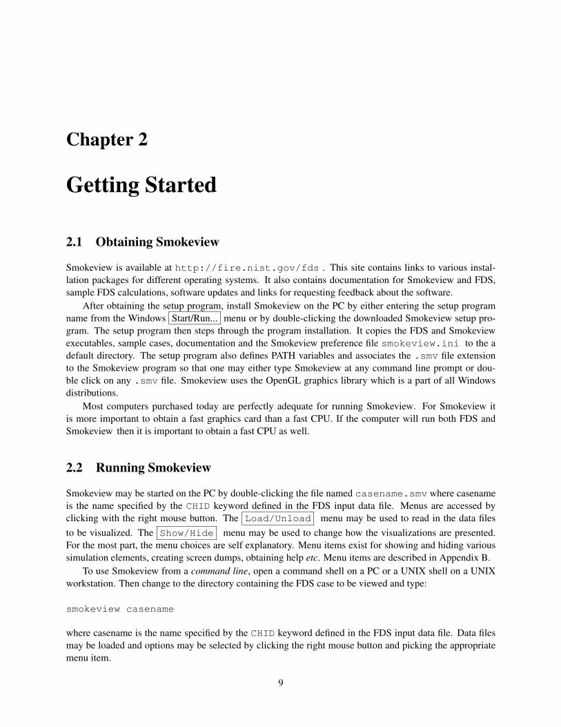
Smokeview is available at http://fire.nist.gov/fds . This site contains links to various instal-lation packages for different operating systems. It also contains documentation for Smokeview and FDS,sample FDS calculations, software updates and links for requesting feedback about the software.
After obtaining the setup program, install Smokeview on the PC by either entering the setup programname from the Windows Start/Run... menu or by double-clicking the downloaded Smokeview setup pro-gram. The setup program then steps through the program installation. It copies the FDS and Smokeviewexecutables, sample cases, documentation and the Smokeview preference file smokeview.ini to the adefault directory. The setup program also defines PATH variables and associates the .smv file extensionto the Smokeview program so that one may either type Smokeview at any command line prompt or dou-ble click on any .smv file. Smokeview uses the OpenGL graphics library which is a part of all Windowsdistributions.
Most computers purchased today are perfectly adequate for running Smokeview. For Smokeview itis more important to obtain a fast graphics card than a fast CPU. If the computer will run both FDS andSmokeview then it is important to obtain a fast CPU as well.
2.2 Running Smokeview
Smokeview may be started on the PC by double-clicking the file named casename.smv where casenameis the name specified by the CHID keyword defined in the FDS input data file. Menus are accessed byclicking with the right mouse button. The Load/Unload menu may be used to read in the data filesto be visualized. The Show/Hide menu may be used to change how the visualizations are presented.For the most part, the menu choices are self explanatory. Menu items exist for showing and hiding varioussimulation elements, creating screen dumps, obtaining help etc. Menu items are described in Appendix B.
To use Smokeview from a command line, open a command shell on a PC or a UNIX shell on a UNIXworkstation. Then change to the directory containing the FDS case to be viewed and type:
smokeview casename
where casename is the name specified by the CHID keyword defined in the FDS input data file. Data filesmay be loaded and options may be selected by clicking the right mouse button and picking the appropriatemenu item.
9

Smokeview opens two windows, one displays the scene and the other displays status information. Clos-ing either window will end the Smokeview session. Multiple copies of Smokeview may be run simultane-ously if the computer has adequate resources.
Normally Smokeview is run during an FDS run, after the run has completed and as an aid in setting upFDS cases by visualizing geometric components such as blockages, vents, sensors, etc. One can then verifythat these modelling elements have been defined and located as intended. One may select the color of theseelements using color parameters in the smokeview.ini to help distinguish one element from another.smokeview.ini file entries are described in section D.1.
Although specific video card brands cannot be recommended, they should be high-end due to Smoke-view’s intensive graphics requirements. These requirements will only increase in the future as more featuresare added. A video card designed to perform well for fancy computer games should do well for Smokeview.Some apparent bugs in Smokeview have been found to be the result of problems found in video cards onolder computers.
10

Chapter 3
Manipulating the Scene Manually
The scene may be manipulated from two points of view, a world or global view and a first person or eyeview. These views may be switched by pressing the “e” key or by selecting the appropriate radio button inthe Motion/View dialog box.
3.1 World View
The scene may be rotated or translated while in world view, either directly with the mouse or by using con-trols contained in the scene movement dialog box. This dialog box is opened from the Dialogs>Motion/Viewmenu item and is illustrated in Figure 3.1. Clicking on the scene and dragging the mouse horizontally, ver-tically or a combination of both results in scene rotation or translation depending upon whether CTRL orALT is depressed or not during mouse movement.
In particular, when modifier keys are not depressed, horizontal or vertical mouse movement results inscene rotation parallel to the XY or YZ plane, respectively. Pressing the CTRL and ALT modifier keys whilemoving the mouse results in scene movement in the following ways:
CTRL key depressed Horizontal mouse movement results in scene translation from side to side alongthe X axis. Vertical mouse movement results in scene translation into and out of the computerscreen along the Y axis.
ALT key depressed Vertical mouse movement results in scene translation along the Z axis. Horizontalmouse movement has no effect on the scene while the ALT key is depressed.
The Motion/View dialog box, illustrated in Figure 3.1 may be used to move the scene in a more con-trolled manner. For example, buttons in the Motion region allows one to translate or rotate the scene. TheHorizontal button allows one to translate the scene horizontally in a left/right or in/out direction while
the Vertical button allows one to translate the scene in an up/down direction.Controls in the View region of the Motion/View dialog box allow one to change the scene magnification
or zoom factor and the projection method used to draw objects (perspective or size preserving). These twoprojection methods differ in how objects are displayed at a distance. A perspective projection for-shortensor draws an object smaller when drawn at a distance. An isometric or size preserving projection on the otherhand draws an objects the same size regardless of where it is drawn in the scene. The projection methoddesired may be selected using the View section of the Motion/View dialog box.
11

Figure 3.1: Motion Dialog Box. Rotate or translate the scene by clicking an arrow and dragging the mouse.The Motion/View Dialog Box is invoked by selecting Dialogs>Motion/View .
12

The zoom and aperture edit boxes allow one to change the magnification of the scene or equiva-lently the angle of view across the scene. The relation between these two parameters is given by
zoom = tan(45◦/2)/ tan(aperture/2)
A default aperture of 45◦ is chosen so that Smokeview scenes have a normal perspective.View may be used to reset the scene back to either an external, internal (to the scene), or previously
saved viewpoint.
Select Rotation Center A pull down list appears in multi-mesh cases allowing one to change the rota-tion center. Therefore one could rotate the scene about the center of the entire physical domainor about the center of any one particular mesh. This is handy when meshes are defined far apart.
Rotation Buttons Rotation buttons are enabled or disabled as appropriate for the mode of scene motion.For example, if about world center - level rotations has been selected, then the Rotate X
and Rotate eye buttons are disabled. A rotation button labelled 90 deg has been addedto allow one to rotate 90 degrees while in eye center mode. This is handy when one wishes tomove down a long corridor precisely parallel to one of the walls. The first click of 90 deg snapsthe view to the closest forward or side direction while each additional click rotates the view 90degrees clockwise.
View Buttons A viewpoint is the combination of a location and a view direction. Several new buttonshave been added to this dialog box to save and restore viewpoints. The scene is manipulated tothe desired orientation then stored by pressing the Add button which adds the new viewpointor the Replace button which replaces this viewpoint with the currently selected one. To changethe view to a currently stored viewpoint, use the Select listbox to select the viewpoint andthe Restore button to activate it. The Delete button may be used to remove a viewpoint fromthe stored list. The Edit text box may be used to change the name or label for the selectedviewpoint. The view at startup button is used to specify the viewpoint that should be set whenSmokeview first starts up.
3.2 Eye View
Radio buttons in the Motion/View dialog box allow one to toggle between world, eye centered and worldlevel rotation scene movement modes. These modes may also be changed by using the “e” key. When ineye center mode, several key mappings have been added, inspired by popular computer games, to allow foreasier movement within the scene. For example, the up and down cursor keys allow one to move forwardor backwards. The left and right cursor keys allow one to rotate left or right. Other keyboard mappings aredescribed in Table 3.1.
13

Table 3.1: Keyboard mappings for eye centered or first person scene movement.
Key Descriptionup/down cursor
move forward/backwardw/sALT + left/right cursor
slide left/righta/dALT + up/down cursor move up/downleft/right cursor rotate left/rightPage Up/Down look up/downHome look levelj toggle between crawling and walkingPressing the SHIFT key while moving, sliding or rotatingresults in a 4x speedup of these actions.
14
Chapter 4
Manipulating the Scene Automatically - TheTouring Option
The touring option allows one to specify arbitrary paths or tours through or around a Smokeview scene. Onemay then view the scenario from the vantage point of an observer moving along one of these paths. A tourmay also be used to observe time dependent portions of the scenario such as blockage/vent openings andclosings. The default view direction is towards the direction of motion. The path tension and start and stoptimes may be changed with the Advanced Settings dialog box illustrated in Figure 4.2b.
When Smokeview starts up it creates a tour, called the circle tour which surrounds the scene. The circletour and a user defined tour are illustrated in Figure 4.1. The circle tour is similar to the Tour menuoption found in earlier versions of Smokeview. The user may modify the circle tour or define their owntours by using the Tour dialog box illustrated in Figure 4.2. The user places several points or keyframes inor around the scene. Smokeview creates a smooth path going through these points.
4.1 Tour Settings
An existing tour may be modified by selecting it from the Select Tour: listbox found in the Edit Tour dialogbox illustrated in Figure 4.2a. A new tour may be created by clicking the New Tour button. A newly createdtour goes through the middle of the Smokeview scene starting at the front left and finishing at the back right.A tour may also be modified by editing the text entries found in the local preference file, casename.ini underthe TOUR keyword.
The speed traversed along the tour is determined by the time value assigned to each keyframe. If theConstant Speed checkbox is checked then these times are determined given the distance between keyframesand the velocity required to traverse the entire path in the specified time as given by the start time and stoptime entries found in the Advanced Settings dialog box illustrated in Figure 4.2b.
Three different methods for viewing the scene may be selected. To view the scene from the point ofview of the selected tour, check the View From Tour Path checkbox. To view the scene from a keyframe(to see the effect of editing changes), select the View From Selected Keyframe checkbox. Uncheckingthese boxes returns control of scene movement to the user.
4.2 Keyframe Settings
A tour is created from a series of keyframes. Each keyframe is specified using time, position and viewdirection. Smokeview interpolates between keyframes using cubic splines to generate the path or tour. An
15

Figure 4.1: Overhead view of townhouse example showing the default Circle tour and a user defined tour.The square dots indicate the keyframe locations. Keyframes may be edited using the Touring or AdvancedTouring dialog boxes.
initial tour is created by pressing the Add Tour button. This tour has two keyframes located at opposite endsof the Smokeview scene. Additional keyframes may be created by selected the Add button.
The position and viewepoint of a keyframe may be adjusted. First it must be selected. A keyframe maybe selected by either clicking it with the left mouse button or by moving through the keyframes using theNext or Previous buttons. The active keyframe changes color from red to green. In Figure 4.1, the active orselected keyframe is at time 40 s. Keyframe positions may then be modified by changing data in the t, X, Yor Z edit boxes. A different view direction may also be set.
A new keyframe is created by clicking the Add button. It is formed by averaging the positions and viewdirections of the current and next keyframes. If the selected keyframe is the last one in the tour then a newkeyframe is added beyond the last keyframe.
A keyframe may be deleted by clicking the Delete button. There is no Delete Tour button. A tour maybe deleted by either deleting all of its keyframes or by deleting its entry in the casename.ini file.
4.3 Advanced Settings
The Advanced Settings dialog box is only necessary if one wishes to override Smokeview’s choice of tensionsettings. This dialog box is opened by clicking the Advanced Settings button contained in the Edit Toursdialog box.
A view direction may be defined at each keyframe by either setting direction angles relative to the path(an azimuth and an elevation angle) or by setting a direction relative to the scene geometry (a cartesian(X,Y,Z) view direction).
Path relative view directions are enabled by default. To define a cartesian view direction, select theX,Y,Z View check box and edit the X, Y and Z View edit boxes to change the view location. To define an
16

a) basic options b) advanced options
Figure 4.2: The Touring dialog boxes may be used to select tours or keyframes, change the position or viewdirection at each keyframe and change the tension of the tour path.
17

path relative view direction, uncheck the X,Y,Z View check box and edit the Azimuth and Elevation editboxes. Checking the View From Selected Keyframe checkbox in the Edit Tours dialog box allows one tosee the effects of the view changes from the keyframe being edited. To see the effect of a change in oneof the keyframe’s parameters, uncheck the View From Selected Keyframe checkbox and position the tourlocator (vertical and horizontal red lines) near the keyframe. The horizontal red line always points in theview direction.
Spline tension settings may also be changed using the Advanced Settings dialog box, though normallythis is not necessary except when one wishes abrupt rather than smooth path changes. Kochanek-Bartels[16]splines (piecewise cubic Hermite polynomials) are used to represent the tour paths.
The cubic Hermite polynomials for each interval are uniquely specified using a function and a derivativeat both endpoints of the interval (i.e. 4 data values). These derivatives are computed in terms of threeparameters referred to as bias, continuity and tension. Each of these parameters range from -1 to 1 with adefault value of 0. The tension value may be set for all keyframes at once (by checking the Global checkbox)or for each keyframe separately. The bias and continuity values are set to zero internally by Smokeview. Atension value of 0 is set by default, a value of 1 results in a linear spline.
4.4 Setting up a tour
The following steps give a simple example of setting up a tour in the townhouse scenario. The tour willbegin at the back of the house, go towards the front door and then end at the top of the stairs. These stepsare illustrated in Figure 4.3.
1. Start by clicking the Dialog>Tours... menu item which opens up the Edit Tours dialog box.
2. Click on the New Tour button in the Edit Tour dialog box. This creates a tour, illustrated in Figure4.3a, starting at the front left of the scene and ending at the back right. This tour has two keyframes.The elevation of each keyframe is halfway between the bottom and top of the scene.
3. Click on the Edit Tour Path checkbox. This activates buttons that allows the user to edit theproperties of each individual keyframe. Click on the square dot at the back of the townhouse. This isthe first keyframe. Change the “Z” value to 1.0. Click on the second dot and change its “Z” value to1.0.
4. Click on the Add button, found inside the Edit Keyframe’s Position panel, three times. This willadd three more key frames to the tour which will be needed so that the path bends up the stairs. Youshould now have five keyframes.
5. Move the first keyframe at the back of the townhouse near the double door by setting X, Y, Z posi-tions to (3.8,-1.0,1.6). Move the last keyframe to the top of the steps by setting X, Y, Z positions to(6.0,3.6,4.1). The path should now look like Figure 4.3b.
6. Move the second, third and fourth keyframes to positions (4.0,4.0,1.6), (4.0,6.8,1.6) and (6.0,6.8,1.6).The path should now look like Figure 4.3c.
7. Click on the Advanced Settings button. Check the Global checkbox and set the All keyframesedit box to 0.5. This tightens up the spline curve reducing the dip near the stairs that occurs with thetension=0.0 setting. The path should now look like Figure 4.3d.
8. Click on the Save Settings button to save the results of your editing changes.
18
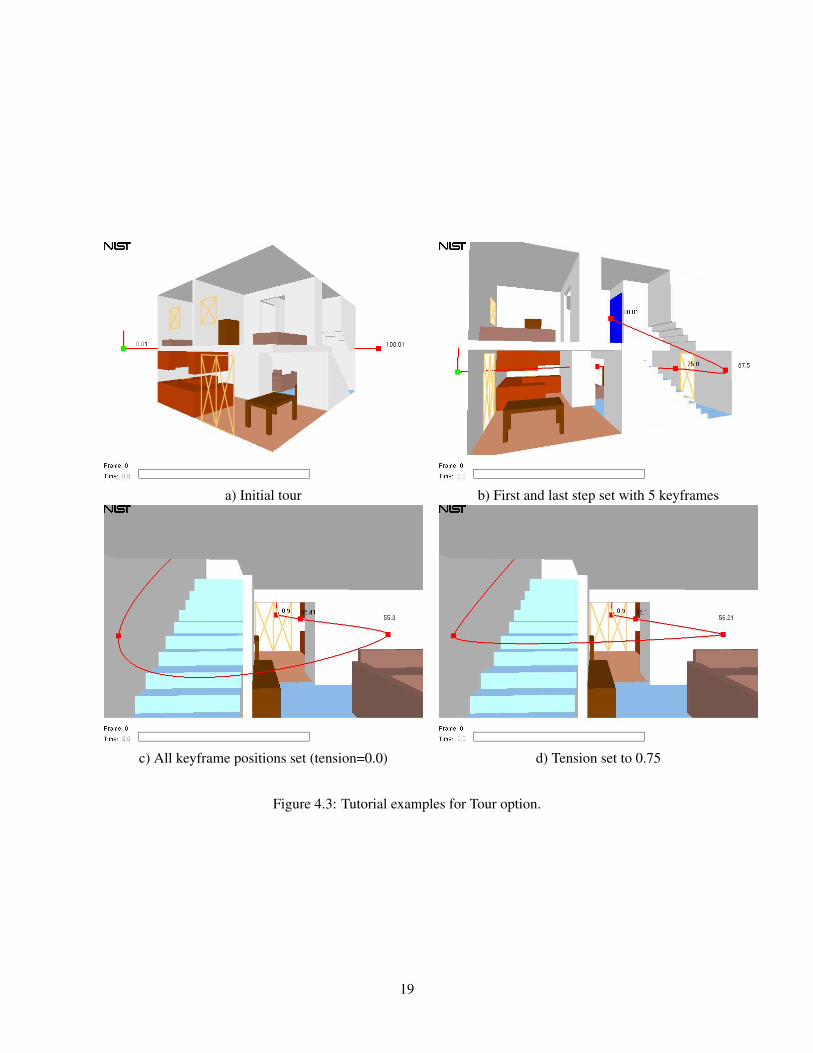
a) Initial tour b) First and last step set with 5 keyframes
c) All keyframe positions set (tension=0.0) d) Tension set to 0.75
Figure 4.3: Tutorial examples for Tour option.
19

9. To see the results of the tour, click on the View From Tour Path check box.
The point of view of the observer on this path is towards the direction of motion. Next the view directionwill be changed to point to the side while the observer is on the first floor.
1. Click on the Advanced Settings button if it is not already open.
2. Uncheck the View From Tour Path checkbox in the tour dialog box and make sure that the X,Y,Z Viewcheckbox is unchecked.
3. Click on the dot representing the first keyframe. Then change Azimuth setting to 90 degrees. To seethe results of the change, go back and check the View From Tour Path checkbox.
4. Uncheck the View From Tour Path checkbox again. Now select the second and third keyframes andchange their azimuth settings to 90 degrees.
With this second set of changes, the observer will look to the side as they pass through the kitchen andliving room. The observer will look straight ahead as they go up the stairs.
20

Chapter 5
Creating Custom Devices
Smokeview draws devices such as heat and smoke detectors, sprinklers, sensors etc. using instructionscontained in a data file. These instructions correspond to OpenGL library calls, the same type of callsSmokeview uses to visualize FDS cases. Smokeview then acts as an OpenGL interpreter executing OpenGLcommands as specified in the device definition file. Efficiency is obtained by compiling these instructionsinto display lists, terminology for an OpenGL construct for storing and efficiently drawing collections ofOpenGL commands.
This section describes how to create new devices. Though all of the examples are given for devices, theintent of this procedure is to be more general allowing Smokeview to draw other types of objects such aspeople walking.
There are two types of instructions: instructions for drawing simple geometric objects such as cubes,disks, spheres etc. and instructions for manipulating these objects through scaling, rotation and translation.Collectively these instructions specify the type, location and orientation of objects used to represent devices.The important feature of this process is that new devices may be designed and drawn without the need tomodify Smokeview.
5.1 Device File Format
The format for an object definition file is given in Figure 5.1. Each device definition consists of one ortwo frames. Devices such as thermocouples which do not activate use just one frame. Other devices suchas sprinklers or smoke detectors which do activate use two frames, the first for normal conditions and thesecond for when the device has activated.
Each definition begins with the DEVICEDEF keyword. The next non-comment line contains a labelnaming the device. Succeeding lines contain one or more commands, each pre-pended by zero or morenumerical arguments. New frames begin with the NEWFRAME keyword. Blank lines may occur anywhere.Definitions may be documented by adding comments following the ‘//’ characters.
Some examples of command/argument pairs are d drawsphere for drawing a sphere of diameter dor x y z translate for translating an object by (x,y,z). Transformation commands are cumulative,each command builds on the effects of the previous command. The push and pop then may be used toisolate these effects by saving and restoring the geometric state. More details may be found in the next twosections.
A simple example of a definition used to draw a sensor along with the corresponding Smokeview viewis given in Figure 5.2. The definition uses just one frame. A sphere is drawn with color yellow and diameter0.038 m. Push and pop commands are not necessary because there is only one object and no transformationsare used.
21
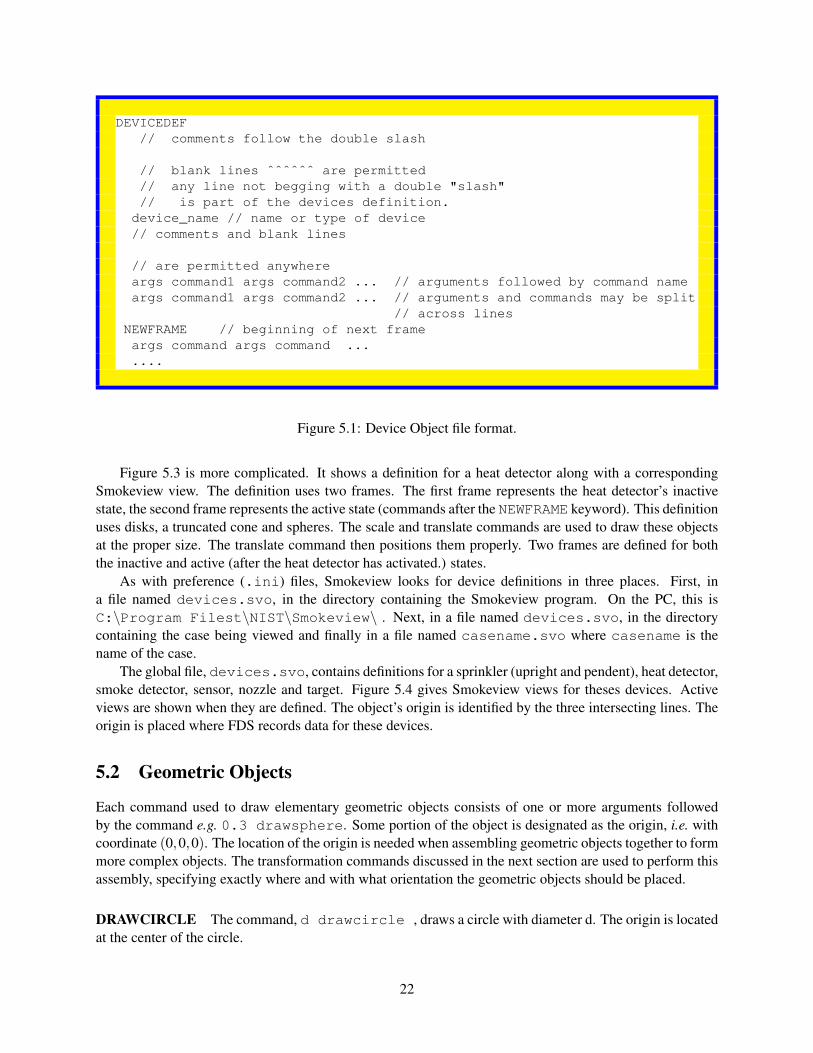
DEVICEDEF// comments follow the double slash
// blank lines ˆˆˆˆˆˆ are permitted// any line not begging with a double "slash"// is part of the devices definition.
device_name // name or type of device// comments and blank lines
// are permitted anywhereargs command1 args command2 ... // arguments followed by command nameargs command1 args command2 ... // arguments and commands may be split
// across linesNEWFRAME // beginning of next frameargs command args command .......
Figure 5.1: Device Object file format.
Figure 5.3 is more complicated. It shows a definition for a heat detector along with a correspondingSmokeview view. The definition uses two frames. The first frame represents the heat detector’s inactivestate, the second frame represents the active state (commands after the NEWFRAME keyword). This definitionuses disks, a truncated cone and spheres. The scale and translate commands are used to draw these objectsat the proper size. The translate command then positions them properly. Two frames are defined for boththe inactive and active (after the heat detector has activated.) states.
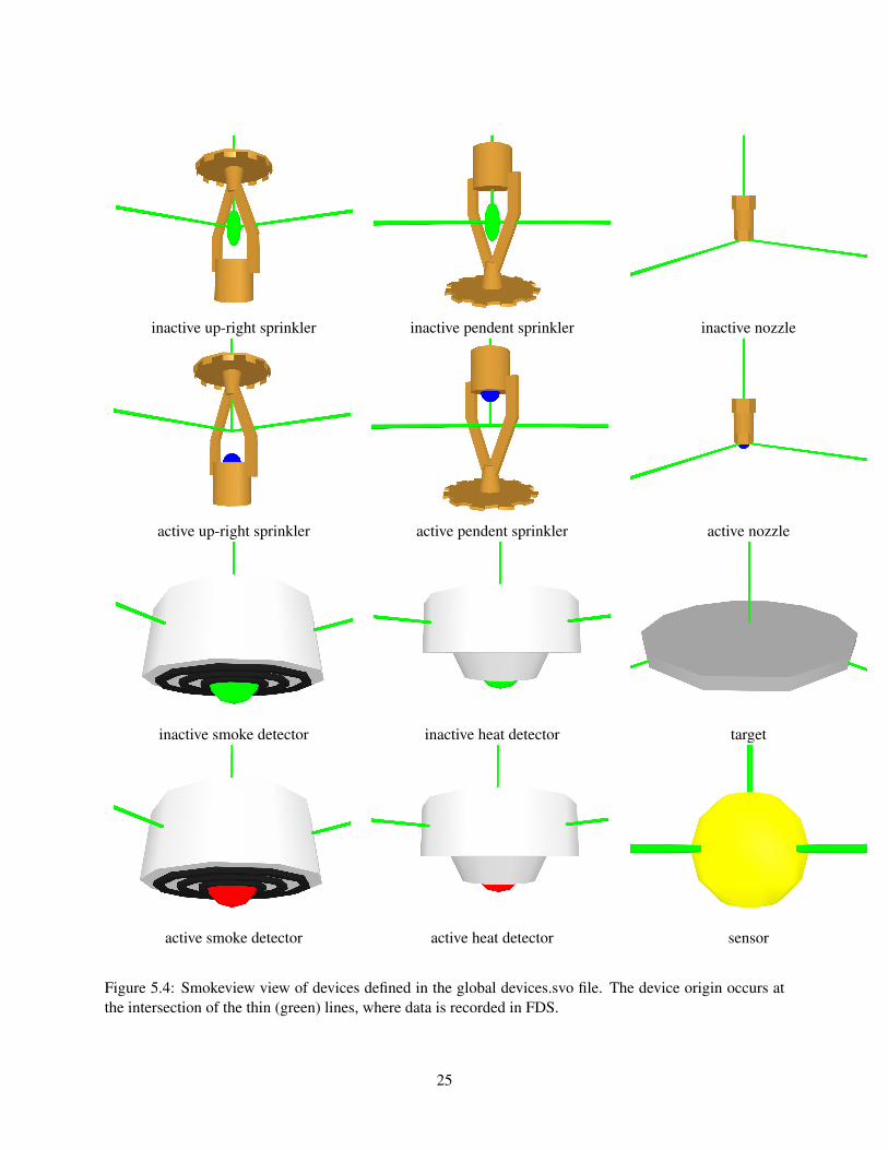
As with preference (.ini) files, Smokeview looks for device definitions in three places. First, ina file named devices.svo, in the directory containing the Smokeview program. On the PC, this isC:\Program Filest\NIST\Smokeview\ . Next, in a file named devices.svo, in the directorycontaining the case being viewed and finally in a file named casename.svo where casename is thename of the case.
The global file, devices.svo, contains definitions for a sprinkler (upright and pendent), heat detector,smoke detector, sensor, nozzle and target. Figure 5.4 gives Smokeview views for theses devices. Activeviews are shown when they are defined. The object’s origin is identified by the three intersecting lines. Theorigin is placed where FDS records data for these devices.
5.2 Geometric Objects
Each command used to draw elementary geometric objects consists of one or more arguments followedby the command e.g. 0.3 drawsphere. Some portion of the object is designated as the origin, i.e. withcoordinate (0,0,0). The location of the origin is needed when assembling geometric objects together to formmore complex objects. The transformation commands discussed in the next section are used to perform thisassembly, specifying exactly where and with what orientation the geometric objects should be placed.
DRAWCIRCLE The command, d drawcircle , draws a circle with diameter d. The origin is locatedat the center of the circle.
22

DEVICEDEFsensor1.0 1.0 0.0 setcolor0.038 drawsphere
Figure 5.2: Instructions for drawing a sensor along with the corresponding Smokeview view.
0.50 0.30 drawcone
DRAWCONE The command, d h drawcone, draws a right circular cone whered is the diameter of the base and h is the height. The origin is located at the center ofthe cone’s base.
0.25 drawcube
DRAWCUBE The command, s drawcube, draws a cube where s is the lengthof the side. The origin is located at the center of the cube. An oblong box, a boxwith different length sides, may be drawn by using scale along with drawcube.For example, 1.0 2.0 4.0 scale 1.0 drawcube creates a box with dimen-sions 1×2×4.
0.25 0.50 drawdisk
DRAWDISK The command, d h drawdisk, draws a circular disk with diame-ter d and height h. The origin is located at the center of the disk’s base.
0.5 0.25 drawhexdisk
DRAWHEXDISK The command, d h drawhexdisk, draws a hexagonal diskwith diameter d and height h. The origin is located at the center of the hexagon’sbase.
DRAWLINE The command, x1 y1 z1 x2 y2 z2 drawline, draws a linebetween the points (x1,y1,z1) and (x2,y2,z2).
23

Heat detector Instructions
DEVICEDEFheat_detector // label, name of device
// The heat detector has three parts// a disk, a truncated disk and a sphere.// The sphere changes color when activated.
0.8 0.8 0.8 setcolor // set color to off whitepush 0.0 0.0 -0.02 translate 0.127 0.04 drawdisk poppush 0.0 0.0 -0.04 translate 0.06 0.08 0.02 drawtrunccone pop0.0 1.0 0.0 setcolorpush 0.0 0.0 -0.03 translate 0.04 drawsphere pop// push and pop are not necessary in the last line// of a frame. Its a good idea though, to prevent// problems if parts are added later.
NEWFRAME // beginning of activated definition0.8 0.8 0.8 setcolorpush 0.0 0.0 -0.02 translate 0.127 0.04 drawdisk poppush 0.0 0.0 -0.04 translate 0.06 0.08 0.02 drawtrunccone pop1.0 0.0 0.0 setcolorpush 0.0 0.0 -0.03 translate 0.04 drawsphere pop
inactive active
Figure 5.3: Instructions for drawing an inactive and active heat detector along with the correspondingSmokeview view.
24
inactive up-right sprinkler inactive pendent sprinkler inactive nozzle
active up-right sprinkler active pendent sprinkler active nozzle
inactive smoke detector inactive heat detector target
active smoke detector active heat detector sensor
Figure 5.4: Smokeview view of devices defined in the global devices.svo file. The device origin occurs atthe intersection of the thin (green) lines, where data is recorded in FDS.
25

0.5 0.1 0.2 1 drawnotchplate 0.5 0.1 0.2 -1 drawnotchplate
DRAWNOTCHPLATE The command, d h nhdir drawnotchplate, draws a notched plate.This object is used to represent a portion of a sprin-kler where d is the plate diameter, h is the plateheight (not including notches), nh is the height ofthe notches and dir indicates the notch orientation(1 for vertical, -1 for horizontal). The origin is located at the center of the plate’s base.
DRAWPOINT The command, drawpoint, draws a point (small square). The command, s setpointsizemay be used to change the size of the point. The default size is 1.0 .
5 0.35 0.15 drawpolydisk
DRAWPOLYDISK The command, n d h drawpolydisk, draws an n-sidedpolygonal disk with diameter d and height h. The origin is located at the center ofthe polygonal disk’s base. The example to the left is a pentagonal disk.
0.3 0.5 0.1 drawring
DRAWRING The command, di do h drawring, draws a ring where di anddo are the inner and outer ring diameters and h is the height of the ring. The originis located at the center of the ring’s base.
0.25 drawsphere
DRAWSPHERE The command, d drawsphere, draws a sphere with diameterd. The origin is located at the center of the sphere. As with an oblong box, anellipsoid may be drawn by using scale along with drawsphere. For example,1.0 2.0 4.0 scale 1.0 drawsphere creates an ellipsoid with semi-majoraxes of length 1, 2 and 4. This is how the ball at the bottom of the heat detector inFigure 5.3a is drawn.
0.5 0.2 0.4 drawtrunccone
DRAWTRUNCCONE The command, d1 d2 h drawtrunccone, drawsa right circular truncated cone where d1 is the diameter of the base, d2 is thediameter of the truncated portion of the cone and h is the height or distancebetween the lower and upper portions of the truncated cone. The origin is locatedat the center of the truncated cone’s base.
5.3 Transformations
As with geometric commands, transformation commands consist of one or more arguments followed by thecommand (except for push and pop which do not require any arguments). Transformation commands areused to change the location and orientation of drawn objects, to save and restore the geometric state and toset attributes such as point size, line width or object color. The rotate and translate commands change theorigin (translate) or orientation of the x,y,z axes (rotate). The PUSH command is then used to save the originor axis orientation while the POP command is used to restore the origin and axis orientation.
26

POP The command, pop, restores the origin and axis orientation saved using a previous pop com-mand. The total number of pop and push commands must be equal, otherwise a fatal error willoccur. Smokeview detects this problem and draws a red sphere instead of the errantly definedobject.
PUSH The command, push, saves the origin and axis orientation. (see above comment about numberof push and pop commands).
ROTATEX The command, r rotatex, rotates objects drawn afterwards r degrees about the x axis.
ROTATEY The command, r rotatey, rotates objects drawn afterwards r degrees about the y axis.
ROTATEZ The command, r rotatez, rotates objects drawn afterwards r degrees about the z axis. Acone or any object for that matter may be drawn upside down by adding a rotatez commandas in 180 rotatez 1.0 0.5 drawcone.
SCALEXYZ The command, x y z scalexyz, stretches objects drawn afterwards by x, y and z re-spectively along the x, y and z axes. The scalexyz along with the drawsphere commandswould be used to draw an ellipsoid by stretching a sphere along one of the axes.
SCALE The command, xyz scale, stretches objects drawn afterwards xyz along each of the x, yand z axes (equivalent to xyz xyz xyz scalexyz ).
SETBW The command, grey setbw, sets the red, green and blue components of color to grey(equivalent to grey grey grey setcolor ). As with the setcolor command, setbw is onlyrequired when the grey level changes, not for each object drawn.
SETCOLOR The command, r g b setcolor, sets the red, green and blue components of the cur-rent color. Any objects drawn afterwards will be drawn with this color. That is, a setcolorcommand is not required for each object part drawn.
SETLINEWIDTH The command, w setlinewidth sets the width of lines drawn with the drawlineand drawcircle commands.
SETPOINTSIZE The command, s setpointsize, sets the size of points drawn with the drawpointcommand.
TRANSLATE The command, x y z translate, translates objects drawn afterwards by x, y andz along the x, y and z axes respectively. Equivalently, one can think of think of x y ztranslate as translating the origin by (-x,-y,-z).
27

28

Part II
Visualization
29


Chapter 6
Realistic or Qualitative Visualization - 3DSmoke
FDS generates several data files visualized by Smokeview. Each file type may be loaded or unloaded usingthe Load/Unload menu described in Appendix B.2. Visualizations produced by these data files aredescribed in this and the following sections. The format used to store each of the data files is given inAppendix D.3.
Visualizing smoke realistically is a daunting challenge for at least three reasons. First, the storagerequirements for describing smoke can easily exceed the disk capacities of present 32 bit operating systemssuch as Linux, i.e. file sizes can easily exceed 2 gigabytes. Second, the computation required both by theCPU and the video card to display each frame can easily exceed 0.1 s, the time corresponding to a 10 frame/sdisplay rate. Third, the physics required to describe smoke and its interactions with itself and surroundinglight sources is complex and computationally intensive. Therefore, approximations and simplifications arerequired to display smoke rapidly.
Smoke visualization techniques such as tracer particles or shaded 2D contours are useful for quantitativeanalysis but not suitable for virtual reality applications, where displays need to be realistic and fast as well asaccurate. The approach taken by Smokeview is to display a series of parallel planes. Each plane is coloredblack (for smoke) with transparency values pre-computed by FDS using time dependent soot densities alsocomputed by FDS corresponding to the grid spacings of the simulation. The transparencies are adjustedin real time by Smokeview to account for differing path lengths through the smoke as the view directionchanges. The graphics hardware then combines the planes together to form one image.
Fire by default is colored a dark shade of orange wherever the computed heat release rate per unit volumeexceeds a user-defined cutoff value. The visual characteristics of fire are not automatically accounted for.The user though may use the 3D Smoke dialog box to change both the color and transparency of the fire forfires that have non-standard colors and opacities.
Figure 6.1 illustrates a visualization of realistic smoke.
31

5.0 s 10.0 s
30.0 s 60.0 s
Figure 6.1: Smoke3d file snapshots at various times in a simulation of a townhouse kitchen fire.
32

Chapter 7
Scientific or Quantitative Visualization
7.1 Tracer Particles and Streaklines - Particle Files
Particle files contain the locations of tracer particles used to visualize the flow field. Figure 7.1 shows severalsnapshots of a developing kitchen fire visualized by using particles where particles are colored black. Ifpresent, sprinkler water droplets would be colored blue. Particles are stored in files ending with the extension.prt51 and are displayed by selecting the particle file entry from the Load/Unload menu.
Streaklines are a technique for showing motion in a still image. Figure 7.2 shows a snapshot of the samekitchen fire using streak lines instead of particles. The streaks begin at 6 s and end at 10 s.
7.2 2D Shaded Contours and Vector Slices - Slice Files
Slice files contain results recorded within a rectangular array of grid points at each recorded time step.Continuously shaded contours are drawn for simulation quantities such as temperature, gas velocity andheat release rate. Figure 7.3 shows several snapshots of a vertical animated slice where the slice is coloredaccording to gas temperature. Slice files have file names with extension .sf and are displayed by selectingthe desired entry from the Load/Unload menu.
To specify in FDS a vertical slice 1.5 m from the y = 0 boundary colored by temperature, use the line:
&SLCF PBY=1.5 QUANTITY=’TEMPERATURE’ /
A more complete list of output quantities may be found in Ref. [3].
New data coloring Smokeview uses a new more precise method for coloring data occurring in slice,boundary and PLOT3D files. This is illustrated in Figure 7.4. The colors are now crisper and sharper, moreaccurately representing the underlying data. This is most noticeable when selecting the colorbar with themouse. As before this causes a portion of the colorbar to turn black and the corresponding region in the sceneto also turn black. Now the black color is accurate to the pixel so this feature could be used to highlightregions of interest. The improved accuracy is a result of the way color interpolations are performed. Thenew method uses a 1D texture map (the colorbar) to color data. Colors are interpolated within the colorbar.Color interpolations with the former method occured within the color cube.
1Particle files created with FDS version 4 and earlier use the .part extension
33

5.0 s 10.0 s
30.0 s 60.0 s
Figure 7.1: Townhouse kitchen fire visualized using tracer particles.
34

Figure 7.2: Townhouse kitchen fire visualized using streak lines. The pin heads shows flow conditions at10 s, the corresponding tails shows conditions earlier from 6 to 10 s.
35

5.0 s 10.0 s
30.0 s 60.0 s
Figure 7.3: Slice file snapshots of shaded temperature contours at various times in a simulation. Thesecontours were generated by adding “&SLCF PBY=1.5, QUANTITY=’TEMPERATURE’ /” to the FDSinput file.
36

interpolate colors interpolate 1D texture color bar
Figure 7.4: Slice file snapshots illustrating old and new method for coloring data.
3D Slice Files The user may now visualize a 3D region of data using slice files. The slices may be movedfrom one plane to the next just as with PLOT3D files (using left/right, up/down cursor keys or page up/pagedown keys). To specify in FDS a cube of data from 1.0 to 2.0 in each of the X, Y and Z directions, use theline:
&SLCF XB=1.0,2.0,1.0,2.0,1.0,2.0 QUANTITY=’TEMPERATURE’ /
Animated vectors are displayed using data contained in two or more slice files. The direction and lengthof the vectors are determined from the U , V and/or W velocity slice files. The vector colors are determinedfrom the file (such as temperature) selected from the Load/Unload menu. The length of the vectors canbe adjusted by pressing the ‘a’ key. For cases with a fine grid, the number of vectors may be overwhelming.Vectors may be skipped by pressing the ‘s’ key. Figure 7.5 shows a sequence of vector slices correspondingto the shaded temperature contours found in Figure 7.3.
To generate the extra velocity files needed to view vector animations, add VECTOR=.TRUE. to theabove &SLCF line to obtain:
&SLCF PBY=1.50,QUANTITY=’TEMPERATURE’,VECTOR=.TRUE. /
7.3 2D Shaded Contours on Solid Surfaces - Boundary Files
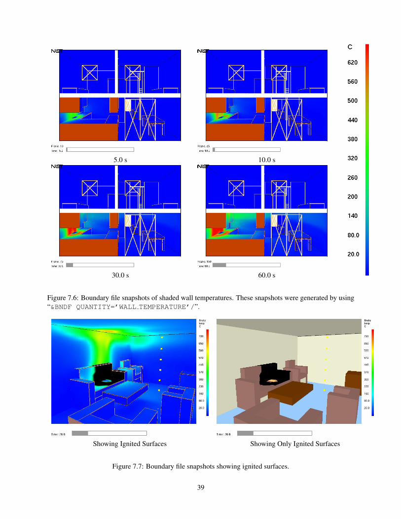
Boundary files contain simulation data recorded at blockage or wall surfaces. Continuously shaded con-tours are drawn for quantities such as wall surface temperature, radiative flux, etc. Figure 7.6 shows sev-eral snapshots of a boundary file animation where the surfaces are colored according to their temperature.Boundary files have file names with extension .bf and are displayed by selecting the desired entry from theLoad/Unload menu.
A boundary file containing wall temperature data may be generated by using:
&BNDF ’WALL_TEMPERATURE’ /
Loading a boundary file is a memory intensive operation. The entire boundary file is read in to determinethe minimum and maximum data values. These bounds are then used to convert four byte floats to one byte
37

5.0 s 10.0 s
30.0 s 60.0 s
Figure 7.5: Vector slice file snapshots of shaded vector plots. These vector plots were generated by using“&SLCF PBY=1.5,QUANTITY=’TEMPERATURE’,VECTOR=.TRUE. /”.
38
5.0 s 10.0 s
30.0 s 60.0 s
Figure 7.6: Boundary file snapshots of shaded wall temperatures. These snapshots were generated by using“&BNDF QUANTITY=’WALL TEMPERATURE’/”.
Showing Ignited Surfaces Showing Only Ignited Surfaces
Figure 7.7: Boundary file snapshots showing ignited surfaces.
39

color indices. To drastically reduce the memory requirements, simply specify the minimum and maximumdata bounds using the Set Bounds dialog box. This should be done before loading the boundary file data.When this is done, memory for the boundary file data is allocated for only one time step rather than for alltime steps.
Highlighting Ignited Surfaces Wall temperature boundary file data may be colored black where temper-atures exceed the ignition temperature of the underlying surface where the ignition temperature is definedon the FDS keyword, &SURF. This is activated by selecting the Show Ignition check box in the Set Boundsdialog box. If one also selects the Show Only Ignition check box then the ignited material is drawn blackbut the rest of the boundary file is not drawn.
A complete list of surface quantities is given in Ref. [3].
7.4 3D Contours - Isosurface Files
The surface where a quantity such as temperature attains a given value is called an isosurface. An isosurfaceis also called a level surface or 3D contour. Isosurface files contain data specifying isosurface locations fora given quantity at one or more levels. These surfaces are represented as triangles. Isosurface files havefile names with extension .iso and are displayed by selecting the desired entry from the Load/Unloadmenu.
Isosurfaces are specified in the FDS input file with the &ISOF keyword. To specify isosurfaces fortemperatures of 30◦C and 100◦C as illustrated in Figure 7.8 add the line:
&ISOF QUANTITY=’TEMPERATURE’, VALUE(1)=30.0, VALUE(2)=100.0 /
to the FDS input file. A complete list of isosurface quantities may be found in Ref. [3]
7.5 Static Data - Plot3D Files
Data stored in Plot3D files use a format developed by NASA [17] and are used by many CFD programs forrepresenting simulation results. Plot3D files store five data values at each grid cell. FDS uses Plot3D filesto store temperature, three components of velocity (U, V, W) and heat release rate. Other quantities may bestored if desired.
An FDS simulation will automatically create Plot3D files at several specified times throughout the sim-ulation. Plot3D data is visualized in three ways: as 2D contours, vector plots and isosurfaces. Figure 7.9ashows an example of a 2D Plot3D contour. Vector plots may be viewed if one or more of the U,V and Wvelocity components are stored in the Plot3D file. The vector length and direction show the direction andrelative speed of the fluid flow. The vector colors show a scalar fluid quantity such as temperature. Figure7.9b shows vectors in a doorway. The vector lengths may be adjusted by depressing the “a” key. Note thehot flow (red color) leaving the fire room in the upper part of the door and the cool flow (blue color) enter-ing fire room in the lower part of the door. Figure 7.10 gives an example of isosurfaces for two differenttemperature levels. Plot3D data are stored in files with extension .q .
40

5.0 s 10.0 s
30.0 s 60.0 s
Figure 7.8:Isosurface file snapshots of temperature levels. The orange surface is drawn where the air/smoke temperatureis 30 ◦C and the white surface is drawn where the air/smoke temperature is 100 ◦C. These snapshots weregenerated by adding “&ISOF QUANTITY=’TEMPERATURE’,VALUE(1)=30.0,VALUE(2)=100.0/” to the FDS input file.
41
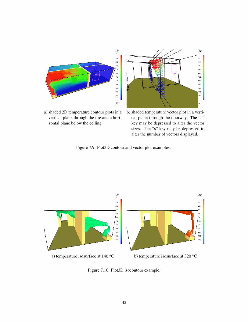
a) shaded 2D temperature contour plots in avertical plane through the fire and a hori-zontal plane below the ceiling
b) shaded temperature vector plot in a verti-cal plane through the doorway. The “a”key may be depressed to alter the vectorsizes. The “s” key may be depressed toalter the number of vectors displayed.
Figure 7.9: Plot3D contour and vector plot examples.
a) temperature isosurface at 140 ◦C b) temperature isosurface at 320 ◦C
Figure 7.10: Plot3D isocontour example.
42

Chapter 8
Visualizing Zone Fire Data
Smokeview may be used to visualize data simulated by a zone fire model. The zone fire model, CFAST[2],creates data files containing geometric information such as room dimensions and orientation, vent locationsetc.. It also outputs modeling quantities such as pressure, layer interface heights, and lower and upperlayer temperatures. Smokeview visualizes the geometric layout of the scenario. It also visualizes the layerinterface heights, upper layer temperature and vent flow. Vent flow is computed internally in Smokeviewusing the same equations and data as used by CFAST. For a given room, pressures , Pi, are computed at anumber of elevations, hi using
Pi = Pf −ρLgmin(hi,yL)−ρU gmax(hi− yL,0)
where Pf is the pressure at the floor (relative to ambient), ρL and ρU are the lower and upper layer densitiescomputed from layer temperatures using the ideal gas law and g is the acceleration of gravity. When densitiesvary continuously with height, this becomes Pi = Pf −
∫ h0 ρ(z)gdz. A pressure difference profile is then
determined using pressures computed on both sides of the given vent.In the visualization, colors represent the gas temperature of the vent flow. The colors change because the
flow may come from either the lower (cooler) or upper (hotter) layer. The length and direction of the coloredvent flow region represents a vent flow speed and direction. Plumes are represented as inverted cones withheights calculated in Smokeview using the same correlation as CFAST and heat release rate data computedby CFAST. A Smokeview view of the one room sample case that comes with the CFAST installation isillustrated in Figure 8.1.
43
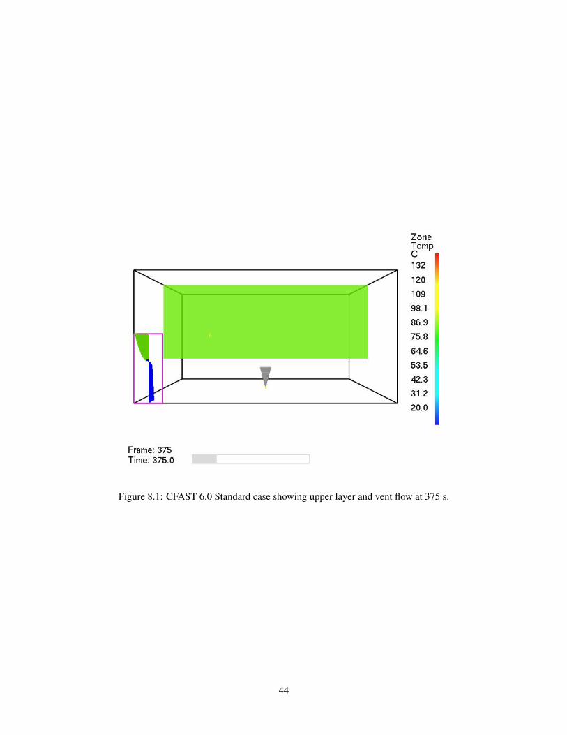
Figure 8.1: CFAST 6.0 Standard case showing upper layer and vent flow at 375 s.
44

Part III
Miscellaneous Topics
45


Chapter 9
Setting Options
9.1 Setting Data Bounds
Normally, Smokeview determines data bounds automatically when it loads data. Sometimes, however, it isdesirable to override Smokeview’s choice. This allows for consistent color shading when displaying severaldata files simultaneously.
The File/Bounds... dialog box is opened from the Dialogs menu. Each file type in Figure 9.1 (slice,particle, Plot3D etc) has a set of radio buttons for selecting the variable type that data bounds are to beapplied to. These variable types are determined from the files generated by FDS and are automaticallyrecorded in the .smv file. The data bounds are set in a pair of edit boxes. Radio buttons adjacent to the editboxes determine what type of bounds should be applied. The Update and Reload buttons are pressedto make the new bounds take effect.
The Plot3D and Slice File portions of the File/Bounds dialog box have additional controls usedto chop or hide data. The settings used in Figure 9.2 were used to generate the ceiling jet visualized inFigure 9.3. Data values less than 140 ◦C are chopped or not drawn in the figure.
Slice file data may be time averaged or smoothed over a user selectable time interval. This option is alsoimplemented from the Slice File section of the File/Bounds dialog box (see Figure 9.2.
The Boundary File portion of the File/Bounds dialog box has an Ignition checkbox which allows oneto visualize when and where the blockage temperature exceeds its ignition temperature.
The bounds dialog for PLOT3D display allows one to select between three different types of contourplots: shaded, stepped and line contours.
9.2 3D Smoke Options
Figure 9.4 allows one to override Smokeview’s choice for several of the 3D smoke parameters. The usermay specify the color of the fire and the gray level of the smoke. A gray level of n where n ranges from 0 to 7results in a color of (2n,2n,2n) where the three components represent red, green and blue contributions. Thehrrpuv cutoff input refers to the heat release rate required at a node before Smokeview will color the nodeas fire rather than smoke. The 50% flame depth allows one to specify the transparency or optical thicknessof the fire (for visualization purposes only). A small value results in opaquely drawn fire while a large valueresults in a transparently drawn fire. The Absorption Parameter setting refers to how the smoke slices aredrawn. The adjust off-center setting causes Smokeview to account for non-axis aligned paths. The adjustoff-center + zero at boundary accounts for off center path lengths and zeros smoke density at boundariesin order to remove graphical artifacts.
47

Figure 9.1: File/Bounds dialog box showing PLOT3D file options. Select a variable and a bounds type checkbox/radio button, then enter a lower and/or upper bound. Data may be excluded from the plot by selecting aTruncate bound. Select type of contour plot to be displayed. Press Reload... or Update for the new boundsto take effect.
Figure 9.2: File/Bounds dialog box showing slice and boundary file options. Select a variable and a boundstype check box/radio button, then enter a lower and/or upper bound. In the slice portion, data may beexcluded from the plot by selecting a Truncate bound. In the boundary portion, ignited materials may behighlighted if a wall temperature boundary file has been saved. Press Reload... or Update for the new boundsto take effect.
48

5.0 s 10.0 s
30.0 s 60.0 s
Figure 9.3: Ceiling jet visualization created by chopping data below 140 ◦C using the Bounds DialogBox as illustrated in Figure 9.2.
49

Figure 9.4: Dialog box for setting 3D smoke options.
9.3 Plot3D Viewing Options
Plot3D files are more complicated to visualize than time dependent files such as particle, slice or boundaryfiles. For example, only the transparency and color characteristics of a time file may be changed. WithPlot3D files however, many attributes may be changed. One may view 2D contours along the X, Y and/orZ axis of up to six1 different simulated quantities, view flow vectors and iso or 3D contours. Plot3D filevisualization is initiated by selecting the desired entry from the Load/Unload Plot3D sub-menu andas with time files one may change color and transparency characteristics.
9.3.1 2D contours
Smokeview displays a 2D contour slice midway along the Y axis by default when a Plot3D file is first loaded,To step the contour slice up by one grid cell along the Y axis, depress the space bar. Similarly to step thecontour slice down by one grid cell along the Y axis, depress the “-” key. To view a contour along either theX or Z axis, depress the x or z keys respectively. Depressing the x, y or z keys while the contour is visiblewill cause it to be hidden. The Plot3D variable viewed may be changed by either depressing the “p” key orby selecting the Solution Variable sub-menu of the Show/Hide menu.
9.3.2 Iso-Contours
Iso-contours also called 3D contours or level surfaces may be viewed by depressing the “i key or by select-ing the Plot3D>3D Contours sub-menu of the Show/Hide menu.
1The FDS software stores temperature, three components of velocity (denoted u, v and w) and heat release per unit volume. Ifat least one velocity component is stored in a Plot3D file, then Smokeview adds speed to the Plot3D variable list.
50

Figure 9.5: Dialog Box for setting miscellaneous Smokeview scene properties.
Figure 9.6: Stereo pair view of a townhouse kitchen fire. To aid in viewing the stereo effect, place a fingerin front of each image. Relax your eyes allowing your two fingers and stereo pair images to merge into one.
9.3.3 Flow vectors
If at least one velocity component is present in the Plot3D file then the “v” key may be depressed in order toview flow vectors. The length and direction of the vector indicates the flow direction and speed. The vectorcolor indicates the value of the currently displayed quantity. A small dot is drawn at the end of the line toindicate flow direction. The vector lengths as drawn may be changed by depressing the “a” key. Vectorplots may be very dense when the grid is finely meshed. The “s” key may be depressed in order to skipvectors. For example, all vectors are displayed by default. If the “s” is depressed then every other vector isskipped.
9.4 Display Options
9.4.1 General
The Display dialog box, illustrated in Figure 9.5, allows one to set various options to control the displayor look of the Smokeview scene. It may be invoked by selecting the Dialogs>Display menu item. Thisdialog box also allows one to show or hide loaded data files.
9.4.2 Stereo
Smokeview implements two methods for displaying images in stereo or 3D. Each method creates two ver-sions of the scene, one version for each eye. In one method, the two images are displayed alternately.
51

Figure 9.7: Dialog box for activating the stereo view option.
Figure 9.8: Clipping dialog box. Clipping entries result in the view shown in Figure 9.9b. Clipping entriesmay be changed individually or selected by mesh number.
Specialized shuttered glasses are synched with the monitor to ensure that the left eye sees only the left eye’sversion of the scene and that the right eye sees only the right eye’s version of the scene. To be effective themonitor requires a refresh rate of at least 120 frames per second (60 frames per second for each eye). Flick-ering is annoyingly noticeable in monitors with slower frame rates. Unfortunately, today’s LCD flat panelmonitors typically do not have refresh rates faster than 60 to 80 frames per second. This method requiresa video card that implements OpenGL QUAD buffering. This Smokeview option can only be enabled fromthe command line by using the -stereo option.
In the second method, Smokeview displays the two images side by side, again one image for each eye.With practice, one can merge the images without requiring specialized equipment, especially if the imagesare small and not separated by a large angle. A trick for seeing the stereo effect is to place a finger fromeach hand in the center of each picture. Then relax your eyes, trying to merge your two fingers together.
Figure 9.6 shows a pair of images of a townhouse kitchen fire. Figure 9.7 shows the dialog box usedto activate this option. If the -stereo command line option was used and the video card supports shutteredstereo display then the shuttered checkbox in the dialog box will be enabled.
9.5 Clipping Scenes
It is difficult to view the interior of a scene when modelling complicated geometries. To alleviate thisproblem, portions of the scene may be hidden or clipped by defining up to six clipping planes. OpenGL
52

a) full scene b) scene clipped to mesh 4
Figure 9.9: Two views of a multi-mesh case. The first view shows the entire scene, the second view showsthe scene clipped to mesh 4. The clipping entries producing the second view are shown in Figure 9.8.
draws the scene on one side of a clipping plane but not the other. In general, a clipping plane may have anyorientation. Smokeview defines two clipping planes for each of the three coordinate axes. The two x axisclipping planes clip regions with x coordinates smaller than an ‘xmin’ clipping value and larger than an ‘xmax’value. The y axis and z axis clipping planes behave similarly. Clipping plane values are specified using theClipping dialog box which is opened by selecting the Dialogs>Clip Geometry menu item. Figure 9.8shows this dialog box with all planes active and values selected for mesh 4 of the scene. The correspondingclipped scene is illustrated in Figure 9.9.
53

54

Chapter 10
Texture Maps
Texture mapping is a technique used by Smokeview to make a scene appear more realistic by pasting im-ages onto obstructions or vents. For example, to apply a wood paneling image to a wall, add the keywordsTEXTURE MAP=’paneling.jpg’, TEXTURE WIDTH=1., TEXTURE HEIGHT=2. to the &SURFline where paneling.jpg is the JPEG file containing the texture map (SGI users should use RGB files in-stead of JPEG) and TEXTURE WIDTH and TEXTURE HEIGHT are the characteristic dimensions ofthe texture map in meters. Note that the image will not appear when Smokeview first starts up. The usermust select the texture maps using the Show/Hide menu.
One can create texture maps using a digital camera or obtain them commercially. The maps should beseamless so that no breaks or seams appear when the maps are tiled on a blockage or vent. This is important,because Smokeview replicates the image as often as necessary to cover the blockage or vent.
When the texture does have a pattern, for example windows or bricks, the keyword TEXTURE ORIGINmay be used to specify where the pattern should begin. For example,
&OBST XB=1.0,2.0,3.0,4.0,5.0,7.0, SURF_ID=’wood paneling’,TEXTURE_ORIGIN=1.0,3.0,5.0 /
will apply paneling to an obstruction whose dimensions are 1 m by 1 m by 2 m, such that the image of thepaneling will be positioned at the point (1.0,3.0,5.0). The default value of TEXTURE ORIGIN is (0,0,0),and the global default can be changed by added a TEXTURE ORIGIN statement to the MISC line.
Figure 10.1 shows a simple application of a texture applied to two different blockages and a vent. Thesame jpeg file was used in two different &SURF lines so that the texture could be stretched by differingamounts (using the TEXTURE WIDTH parameter.) The FDS data file used to create this Figure follows.
&HEAD CHID=’sillytexture’, TITLE=’Silly Test Case’ /&MISC TEXTURE_ORIGIN=0.1,0.1,0.1 /
&MESH IJK=20,20,02, XB=0.0,1.0,0.0,1.0,0.0,1.0 /&TIME TWFIN=0. /&SURF ID = ’TEXTURE 1’
TEXTURE_MAP= ’nistleft.jpg’TEXTURE_WIDTH=0.6TEXTURE_HEIGHT=0.2 /
&SURF ID = ’TEXTURE 2’TEXTURE_MAP= ’nistleft.jpg’TEXTURE_WIDTH=0.4
55

Figure 10.1: Texture map example. The same texture was applied to two different blockages and a vent(with different widths) by assigning different TEXTURE WIDTH parameters in the input file.
TEXTURE_HEIGHT=0.2 /&OBST XB=0.1,0.3,0.1,0.7,0.1,0.3, SURF_ID=’TEXTURE 1’ /&OBST XB=0.5,0.9,0.3,0.7,0.1,0.5, SURF_ID=’TEXTURE 2’,
TEXTURE_ORIGIN=0.5,0.3,0.1 /
&VENT XB=0.0,0.0,0.2,0.8,0.2,0.4, SURF_ID=’TEXTURE 1’,TEXTURE_ORIGIN=0.0,0.2,0.2 /
&VENT XB=0.3,0.9,0.0,0.0,0.3,0.5, SURF_ID=’TEXTURE 1’,TEXTURE_ORIGIN=0.9,0.0,0.3 /
56

Chapter 11
Using Smokeview to Debug FDS Input Files
One of the most difficult tasks in setting up an FDS input file is defining the geometry (blockages, ventlocations etc) properly. Smokeview may be used to debug FDS input files by making short model runsand observing whether blockages, vents and other geometric features of a model run are located correctly.Blockages may then be created or changed. This is done with the Edit Geometry dialog box called from theDialogs menu.
The following is a general procedure for identifying problems in FDS input files. Assume that the FDSinput data file is named testcase1.fds.
1. In the FDS input file, set the stop time to 0.0 using TWFIN=0.0 on the &TIME line. This causes FDSto read the input file and create a .smv file without performing lengthy startup calculations.
2. Run the FDS model (for details see the FDS User’s Guide[3])
FDS creates a file named testcase1.smv containing information that Smokeview uses to visual-ize model.
3. To visualize the model, open testcase1.smv with Smokeview by either typing smokeviewtestcase1 at a command shell prompt or if on the PC by double-clicking the file testcase1.smv.
4. Make corrections to the FDS data file, if necessary. Using the COLOR or RGB option of the OBSTkeyword to more easily identify blockages to be edited. For example, to change a blockage’s color tored use:
&OBST XB=0.0,1.0,0.0,1.0,0.0,1.0, COLOR=’RED’ /
or
&OBST XB=0.0,1.0,0.0,1.0,0.0,1.0 RGB=255,0,0 /
Save testcase1.fds file and go back to step 2.
5. If corrections are unnecessary, then change the TWFIN keyword back to the desired final simulationtime, remove any unnecessary FDS COLOR keywords and run the case.
57

Figure 11.1: Blockage Edit Dialog Box. Click on ‘New’ to create a new blockage or click on an existingblockage in the Smokeview scene to change its size or location. Change the size or location by enteringblockage bounds directly or clicking an ‘arrow’ and/or direction buttons. Note, the blockage editor does notwork when clipping planes are active.
11.1 Examining and/or Editing Blockages
Blockages may be examined or changed by selecting the menu item Dialogs/Edit Geometry whichopens up the dialog box illustrated in Figure 11.1. Text edit boxes allow one to define comments (any textto the right of the closing “/” on an &OBST line and pull down menus for linking surfaces (&SURF lines)to obstructions. The surface choices are obtained from the input file or the database file if one is specified inthe input file for FDS 4 and earlier cases.
Note, the blockage editor does not work when clipping planes are active.The user may associate one, three or six surfaces with an obstruction. If the 3 wall radio button is
selected then materials for the top (upper surface), sides (vertical surfaces) and bottom (lower surface) maybe specified. The color check box allows the input or default color (manilla) to be displayed on blockagesurfaces.
Associating unique colors with each surface allows the user to quickly determine whether blockages aredefined with the proper surfaces. One can then verify that these modeling elements have been defined andpositioned as intended.
The blockage editor works on one mesh at a time. For multi-mesh cases, use the Mesh list-box to selectthe desired mesh or simply click on a blockage in the mesh to switch to that mesh. The pull-down menu isnecessary for meshes without blockages.
Position coordinates entered into the text boxes are snapped to the nearest grid line. Materials appearingunder Surface Type come from those materials defined in either the input data file or the database file.Either one, three or six wall properties can be entered by selecting the appropriate radio button.
58
Chapter 12
Making Movies
A movie can be made of a Smokeview animation by converting the visualized scene into a series of PNGor JPEG files, one file for each time step and then combining the individual images together into one moviefile. More specifically:
1. Set up Smokeview by orienting the scene and loading the desired data files.
2. Select the Options/Render menu and pick the desired frame skip value. The more frames you includein the animation, the smoother it will look. Of course more frames result in larger file sizes. Choosefewer frames if the movie is to appear on a web site.
3. Use a program such as the Antechinus Media Editor (http://www.c-point.com ), Apple Quick-time Pro (http://www.quicktime.com ), or Adobe Premiere Pro (http://www.adobe.com), to assemble the JPEGS or PNGS rendered in the previous step into a movie file.
The default Smokeview image size is 640× 480 . This size is fine if the movie is to appear in a pre-sentation located on a local hard disk. If the movie is to be placed on a web site then care needs to betaken to insure that the generated movie file is a reasonable size. Two suggestions are to reduce the imagesize to 320× 240 or smaller by modifying the WINDOWWIDTH and WINDOWHEIGHT smokeview.inikeywords and to reduce the number of frames to 300 or less by skipping intermediate frames via theOptions/Render menu.
Sometimes when copying or capturing a Smokeview scene it is desirable, or even necessary, to havea margin around the scene. This is because the capturing system does not include the entire scene butitself captures an indented portion of the scene. To indent the scene, either press the “h” key or select theOption>Viewpoint>Offset Window menu item. The default indentation is 45 pixels. This may be changed
by adding/editing the WINDOW OFFSET keyword in the smokeview.ini file.Note, the Smokeview animation must be running when the render command is selected or only one
frame will be saved instead of the entire image sequence.
59

60

Chapter 13
Annotating the Scene
Smokeview rendered JPEG or PNG image files may be annotated with any package that edits these typesof files. Tick marks and label annotation can be placed within the 3D scene and moved around as the sceneis moved. This would be difficult to duplicate with an external image editor. In addition, axis labels aredisplayed, if desired, by selecting the tt Axis checkbox in the Display dialog box illustrated in Figure 9.5.
The current release of FDS places tick marks and labels documenting the scene dimensions. To replaceor customize these annotations add the TICK keyword to a .smv file using the following format:
TICKSxb yb zb xe ye ze nticksticklength tickdir r g b tickwidth
where xb, yb, and zb are the x, y and z coordinates of the first tick; xe, ye and ze are the x, y and zcoordinates of the last tick and nticks is the number of ticks. The coordinate dimensions are in physicalunits, the same units used to set up the FDS geometry. The parameter ticklength specifies the lengh ofthe tick in physical units. The parameter tickdir specifies the tick direction. For example 1(-1) placesticks in the positive(negative) x direction. Similarly, 2(-2) and 3(-3) place ticks in the positive(negative) yand positive(negative) z directions.
The color parameters r, g and b are the red, green and blue components of the tick color each rangingfrom 0.0 to 1.0. The foreground color (white by default) may be set by setting any or all of the r, g andb components to a negative number. The tickwidth parameter specifies tick width in pixels. Fractionalwidths may be specified.
The LABEL keyword allows a text string to be added within a Smokeview scene. The label color andstart and stop appearance time may also be specified. The format is given by
LABELSx y z r g b tstart tstoplabel
where (x, y, z) is the label location in cartesian coordinates and r, g, b are the red, green and bluecolor components ranging from 0.0 to 1.0. Again, if a negative value is specified then the foreground colorwill be used instead (white is the default). The parameters, tstart and tstop indicate the time intervalwhen the label is visible. The text string is specified on the next line (label).
Figure 13.1 shows how the LABEL and TICKS keywords can be used together to create a ruler withmajor and minor tick marks. These ticks and labels were created using:
61
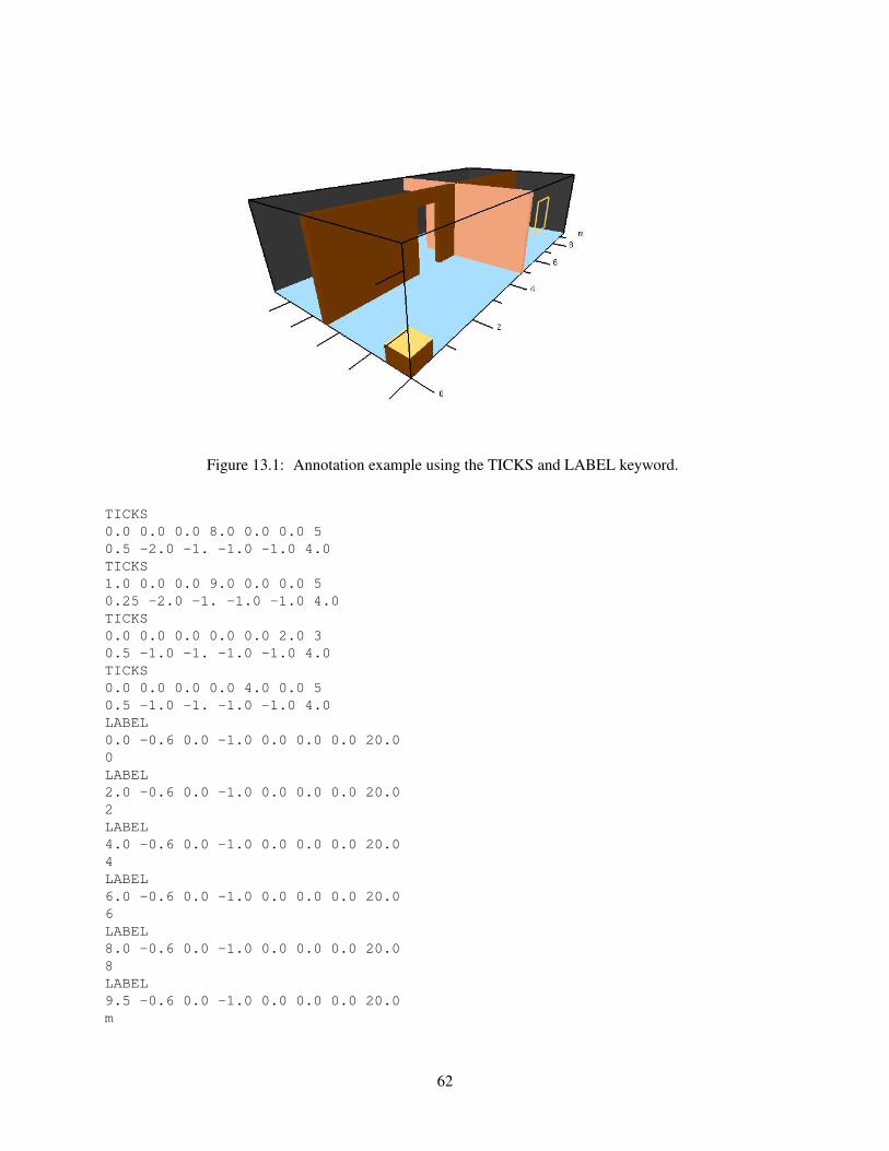
Figure 13.1: Annotation example using the TICKS and LABEL keyword.
TICKS0.0 0.0 0.0 8.0 0.0 0.0 50.5 -2.0 -1. -1.0 -1.0 4.0TICKS1.0 0.0 0.0 9.0 0.0 0.0 50.25 -2.0 -1. -1.0 -1.0 4.0TICKS0.0 0.0 0.0 0.0 0.0 2.0 30.5 -1.0 -1. -1.0 -1.0 4.0TICKS0.0 0.0 0.0 0.0 4.0 0.0 50.5 -1.0 -1. -1.0 -1.0 4.0LABEL0.0 -0.6 0.0 -1.0 0.0 0.0 0.0 20.00LABEL2.0 -0.6 0.0 -1.0 0.0 0.0 0.0 20.02LABEL4.0 -0.6 0.0 -1.0 0.0 0.0 0.0 20.04LABEL6.0 -0.6 0.0 -1.0 0.0 0.0 0.0 20.06LABEL8.0 -0.6 0.0 -1.0 0.0 0.0 0.0 20.08LABEL9.5 -0.6 0.0 -1.0 0.0 0.0 0.0 20.0m
62

Chapter 14
Compression - Using Smokezip to reduceFDS file sizes
3D smoke, boundary and slice files may now be compressed using the stand-alone program smokezip orfrom within Smokeview using the compression menu item found on the Load/Unload menu. Filecompression may also be activated from the Compressions, Autoload section of the File Bounds dia-log box illustrated in Figure 14.1. Compression is performed using the ZLIB compression library (seehttp://www.zlib.org ). When using Smokeview, compression is performed in the background al-lowing one to continue visualization. Smokeview adds the label ZLIB to Load menu entries for any files thathave been compressed. Smokezip adds the extension svz to the corresponding compressed file name.
The usage for Smokezip is
smokezip 1.0 - Mar 12 2006
Compresses Smokeview 3D smoke and boundary files
smokezip [-f] [-s sourcedir] [-d destdir] [-c] casename [destdir]
-f - overwrites compressed boundary and 3D smoke files
-d destdir - if specified will copy compressed files (and files needed by Smokeview to view the case) tothe directory destdir
-s sourcedir - if specified assumes all files are in directory sourcedir
-c - clean or remove all compressed files
casename - Smokeview .smv file
Smokezip uses min and max specifications found in the casename.ini file to determine how to mapthe four byte floating point data found in the boundary files to one byte color indices used by Smokeview.Smokezip uses percentile min and max bounds if the casename.ini file does not exist. The algorithms fordetermining the data mappings used by Smokeview and Smokezip are identical so it should result in thesame views.
63
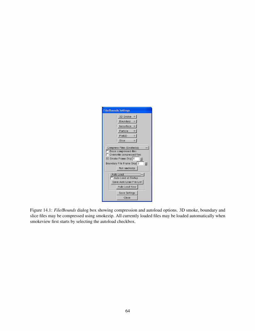
Figure 14.1: File/Bounds dialog box showing compression and autoload options. 3D smoke, boundary andslice files may be compressed using smokezip. All currently loaded files may be loaded automatically whensmokeview first starts by selecting the autoload checkbox.
64

Chapter 15
Summary
Often fire modeling is looked upon with skepticism because of the perception that eye-catching imagesshroud the underlying physics. However, if the visualization is done well, it can be used to assess the qualityof the simulation technique. The user of FDS chooses a numerical grid on which to discretize the governingequations. The more grid cells, the better but more time-consuming the simulation. The payoff for investingin faster computers and running bigger calculations is the proportional gain in calculation accuracy andrealism manifested by the images. There is no better way to demonstrate the quality of the calculation thanby showing the realistic behavior of the fire.
Up to now, most visualization techniques have provided useful ways of analyzing the output of a calcu-lation, like contour and streamline plots, without much concern for realism. A rainbow-colored contour mapslicing down through the middle of a room is fine for researchers, but for those who are only accustomed tolooking at real smoke-filled rooms, it may not have as much meaning. Good visualization needs to provideas much information as the rainbow contour map but in a way that speaks to modelers and non-modelersalike. A good example is smoke visibility. Unlike temperature or species concentration, smoke visibility isnot a local quantity but rather depends on the viewpoint of the eye and the depth of field. Advanced simula-tors and games create the illusion of smoke or fog in ways that are not unlike the techniques employed byfire models to handle thermal radiation. The visualization of smoke and fire by Smokeview is an exampleof the graphics hardware and software actually computing results rather than just drawing pretty pictures.A common concern in the design of smoke control systems is whether or not building occupants will beable to see exit signs at various stages of a fire. FDS can predict the amount of soot is located at any givenpoint, but that doesn’t answer the question. The harder task is to compute on the fly within the visualizationprogram what the occupant would see and not see. In this sense, Smokeview is not merely a post-processor,but rather an integral part of the analysis.
65

66

Bibliography
[1] K.B. McGrattan, S. Hostikka, J.E. Floyd, H.R. Baum, and R.G. Rehm. Fire Dynamics Simulator (Ver-sion 5), Technical Reference Guide. NIST Special Publication 1018-5, National Institute of Standardsand Technology, Gaithersburg, Maryland, October 2007.
[2] W. W. Jones, R. D. Peacock, G. P. Forney, and P. A. Reneke. CFAST, Consolidated Model of FireGrowth and Smoke Transport (Version 5. technical reference guide. NIST Special Publication 1030,National Institute of Standards and Technology, Gaithersburg, Maryland, October 2004.
[3] K.B. McGrattan, B.W. Klein, S. Hostikka, and J.E. Floyd. Fire Dynamics Simulator (Version 5),User’s Guide. NIST Special Publication 1019-5, National Institute of Standards and Technology,Gaithersburg, Maryland, October 2007.
[4] D. Madrzykowski and R.L. Vettori. Simulation of the Dynamics of the Fire at 3146 Cherry Road NE,Washington, DC May 30, 1999. Technical Report NISTIR 6510, Gaithersburg, Maryland, April 2000.URL: http://fire.nist.gov/6510 .
[5] D. Madrzykowski, G.P. Forney, and W.D. Walton. Simulation of the Dynamics of a Fire in a Two-StoryDuplex, Iowa, December 22, 1999. Technical Report NISTIR 6854, Gaithersburg, Maryland, January2002. URL: http://www.fire.nist.gov/bfrlpubs/duplex/duplex.htm .
[6] R.L. Vettori, D. Madrzykowski, and W.D. Walton. Simulation of the Dynamics of a Fire in a One-StoryRestaurant – Texas, February 14, 2000. Technical Report NISTIR 6923, Gaithersburg, Maryland,October 2002.
[7] R.G. Rehm, W.M. Pitts, Baum H.R., Evans D.D., K. Prasad, K.B. McGrattan, and G.P. Forney. InitialModel for Fires in the World Trade Center Towers. Technical Report NISTIR 6879, Gaithersburg,Maryland, May 2002.
[8] Mason Woo, Jackie Neider, Tom Davis, and Dave Shreiner. OpenGL Programming Guide. Addison-Wesley, Reading, Massachussets, 3 edition, 1999.
[9] Mark J. Kilgard. OpenGL Programming for the X Window System. Addison-Wesley Developers Press,Reading, Massachussets, 1996.
[10] Thomas Boutell. CGI Programming in C & Perl. Addison-Wesley Publishing Company, Reading,Massachussets, 1996.
[11] Thomas Boutell. GD version 2.0.7, http://www.boutell.com/gd/, November 2002.
[12] Guy Eric Schalnat, Andreas Dilger, and Glenn Randers-Pehrson. libpng version 1.2.5,http://www.libpng.org/pub/png/, November 2002.
67

[13] JPEG version 6b, http://www.ijg.org/.
[14] Jean loup Gailly and Mark Adler. zlib version 1.1.4, http://www.gzip.org/zlib/, November 2002.
[15] Paul Rademacher. GLUI version 2.1, http://www.cs.unc.edu/ rademach/glui/.
[16] Tomas Akenine-Moller and Eric Haines. Real-Time Rendering. A K Peters, Ltd., Natick, Mas-sachusetts, 2nd edition, 2002.
[17] Pamela P. Walatka and Pieter G. Buning. PLOT3D User’s Manual, version 3.5. NASA TechnicalMemorandum 101067, NASA, 1989.
68
Appendix A
Command Line Options
Smokeview may be run from a command shell. Furthermore, command line options may be invoked inorder to alter Smokeview’s startup behavior. Normally these options are not necessary. However, they maybe used for cases with very large particle files or to generate a preference or customization file. To obtain alist of command line options, type:
smokeview -help
without any arguments which results in output similar to:
Smokeview 5.0.0_634 - Sep 19 2007Visualize fire/smoke flow simulations. All parameters are optional.
Usage:
smokeview casename -points m -frames n -ini -part -nopart -stereo
where
casename = project id (file names without the extension)m = maximum number of particles. Default=50000000n = maximum number of particle frames. Default=5001
-ini = output default smokeview parameters to smokeview.ini-part = load particle file if present
-nopart = do not load particle file-stereo = activate stereo mode (if supported)-build = show pre-preprocessing directives used to build smokeview
The -nopart option is used to prevent a particle file from being loaded at startup. The -points and-frames options are used to load more than the default 5,000,000 points or 500 frames where a frame isdata for one time step. To load up to 6,000,000 points and 1000 frames then type:
smokeview casename -points 6000000 -frames 1000
where in both cases casename is the basename of the FDS output files. The same effect may be achievedby using:
69

MAXPOINTS6000000MAXFRAMES1000
in the smokeview.ini or casename.ini file. This file may be created with the -ini option andcontains many other customizable Smokeview parameters. The -benchmark option is used to measurethe performance of Smokeview. The -benchmark option causes Smokeview to produce precise timingsby outputting frame rates based upon one cycle through the timing loop rather than using moving averages.The -stereo option may used to access stereo hardware (often called quad buffering) if it is available.
70

Appendix B
Menu Options
The design philosophy used to develop Smokeview has been to avoid complicated, non-portable user inter-faces that are costly to implement. As a result, most of the development effort has gone into the visualization(display of particle flow, contour plots etc) rather than user interface design and implementation. Smoke-view’s pop-up menus are implemented with GLUT[9], the graphics library utility toolkit. The user interactswith Smokeview via 1) menus, 2) keyboard shortcuts and 3) the preference file (smokeview.ini orcasename.ini).
A pop up menu is displayed when the right mouse is clicked anywhere within the scene. The mainmenu options as illustrated in Figure B.1 are: Load/Unload Show/Hide , Options , Dialogs
Tours , View and Help . Several of these menu options have sub-menus. These menus are describedin the following sections.
B.1 Main Menu Items
Load/Unload This menu option allows one to load or unload particle, isosurface, vector slice, slice,Plot3D or boundary files. These time dependent files may be viewed simultaneously, but notconcurrently with the time independent Plot3D files. However, one boundary or one Plot3Dfile per mesh may be viewed at a time. Multiple slices for the same variable may be viewedsimultaneously. This menu may also be used to load and create preference files .ini filesand to re-read the .smv file. For more details see Appendix B.2.
Show/Hide This menu item allows one to show or hide the loaded data files and various scene attributessuch as time/color bars, internal blockages etc. As a file type is shown or hidden (or loaded andunloaded), the color and time bars are changed to reflect the currently visible data files. Moredetails are given in Appendix B.3.
Options This menu allows one to specify various smokeview options such as specifying frame rates,rendering the screen to a PNG or JPEG file, changing font sizes, selecting dialog boxes etc.
Dialogs This menu allows one to open/close various dialog boxes for setting data bounds, controllingthe look of the 3D smoke, specifying clip planes etc.
Tour This menu displays a list of tours stored in the casename.ini preference file. The manualtour gives control back to the user. Tours may be defined using the Tour dialog box.
View Resets the simulation scene to an alternate view. The three choices are 1) exterior view, 2)interior view or a 3) user defined view. A viewpoint may be saved by using this menu or by
71

Figure B.1: Main Menu.
using the Viewpoint sub-menu of the Options menu. If a time file is visible then twosub-menus occur allowing one to reset the view back to the original position or the time barback to the initial time.
Help Displays a list and explanation of keyboard equivalent commands.
B.2 Load/Unload
Six types of files may be visualized with Smokeview. These files are loaded using the LOAD/UNLOADmenus as illustrated in Figure B.2. They are particle, vector slice, slice, boundary, isosurface and Plot3Dfiles. Note that vector slice animations use two or more slice files to display the animated vector slices.The format of the data contained in these files is described in Appendix D.3. A sub-menu is present underLoad/Unload for each file type generated for the simulation. Selecting one of the files appearing in
the sub-menu causes it to be loaded and then displayed. The data may be unloaded or freed by selecting anUnload menu item appearing under the file list. Selecting Unload All as expected will unload all
files. To hide a data file, select the Show/Hide menu option corresponding to the file type to be hidden.The Smokeview .smv file contains information about all data files appearing in the Load/Unload
menu item. The FDS field modelling software creates this file. (See Appendix D.2 for documentation onthe format of this file).
The character “*” occurring before a file name in one of the sub-menus indicates that the file has alreadybeen loaded. If the file below is loaded but not visible, then use the appropriate Show/Hide option tomake it visible.
Open Smokeview (.smv) This menu item allows one (on the PC) to use an open file dialog box to opena Smokeview scene (file with .smv extension). This menu is only active when one starts upSmokeview without first specifying a file. (One cannot open a new Smokeview file after one
72

Figure B.2: Load/Unload Menu.
73

has already been opened.)
3D Smoke File (.s3d) This menu item allows one to load realistic smoke, fire or water spray files.
Slice File (.sf) This menu item gives the name and location of all available slice files and also theoption to unload the currently loaded slice files.
Multi-Slice File (.sf) This menu item allows one to load all slices occurring in one plane (within agrid cell) simultaneously. It also gives the option to unload the currently loaded multi-slices.
Vector Slice File (.sf) This menu item gives the name of all slice files that have one or more associatedU, V and/or W velocity slice files. These slice files must be defined for the same region (or slice)in the simulation.
Multi-Vector Slice File (.sf) This menu item allows one to load all vector slices occurring in oneplane (within a grid cell) simultaneously. It also gives the option to unload the currently loadedmulti-slices.
Isosurface File (.iso) This menu item gives the name of all isosurface files and also the option tounload the currently loaded isosurface file.
Boundary File (.bf) This menu item gives the name of all boundary files and also the option to unloadthe currently loaded boundary file.
Particle File (.part) This menu item gives the name of all particle file and also the option to unloadthe currently loaded particle file.
Plot3D File (.q) This menu item gives the name of all Plot3D files and also the option to unload thecurrently loaded Plot3D file.
Preference File (.ini) The INI or preference file contains configuration parameters that may be usedto customize Smokeview’s appearance and behavior. This menu item allows one to create (oroverwrite) a preference file named either smokeview.ini or casename.ini. A prefer-ence file contains parameter settings for defining how Smokeview visualizes data. This file maybe edited and re-read while Smokeview is running.
Compression 3D smoke and boundary files may be compressed using this menu item.
Show File Names Load and Unload menus by default are specified using the location and type of visualto be displayed. This menu item adds file names to the Load and Unload menus.
Reload This menu item allows one to reload files at immediately or at intervals of 1, 5 or 10 minutes.The u key may used to reload files from the keyboard. This is useful when using Smokeview todisplay a case that is currently running in FDS.
Unload All This option causes all data files to be unloaded.
B.3 Show/Hide
The Show/Hide menu item allows one to show or hide various parts of the simulation. This menuitem contains sub-menus for Particles, Boundary, Animated Slice, Plot3D 2D and 3D contours, sensors
74

Figure B.3: Geometry Menu.
(thermocouples, heat detectors and sprinklers), Color and time Bars and Geometry. These menu items onlyappear if they pertain to the simulation. For example the Particles sub-menu only appears if a particlefile has been loaded. Similarly, the Plot3D contouring sub-menus only appear if a Plot3D file hasbeen loaded. The “*” character is used to indicate whether the visualization feature corresponding to themenu item is set or active.
B.3.1 Geometry Options
The Geometry menu is illustrated in Figure B.3.
Blockages Blockage sub-menus are divided into two groups. The first group allows the user to changehow blockage appear ( Defined in Input File , Normal , Outline , Hidden ).
The second group allows the user to change where blockages are located (actual or re-quested). The Actual sub-menu positions blockages as computed by FDS (along grid lines).The Requested sub-menu positions blockages at locations as specified in the input file.If the dx2dxf conversion program was used to convert a CAD drawing to input compatiblewith FDS and Smokeview then a third menu option appears, CAD . This option displays theSmokeview scene in a form similar to the original CAD drawing.
Grid This option allows one to visualize the grid used to perform the numerical calculations. Oneselects xy plane , xz plane or yz plane to visualize a single plane or Show All ,
Hide All to show or hide all grids. (Keyboard shortcut: g)
Outline Show or hide the outline that frames the simulation scene.
Floor Show or hide the floor.
Ceiling Show or hide the ceiling.
Vents Show or hide the vents.
Walls Show or hide the walls.
75

Show All Show all geometric features described above.
Hide All Hide all geometric features described above.
B.3.2 Animated Surface
This menu allows one to control the way isosurfaces are displayed. An isosurface is represented in Smoke-view as a collection of triangles. Each triangle consists of three edges and three vertices.
Solid Display the isosurface by shading the triangles.
Outline Display the isosurface by only showing the triangle edges.
Points Display the isosurface by only showing the triangle vertices.
quantity levels Display the desired isosurface level (when more than one isosurface is stored in an iso-surface file).
Smooth Display the isosurface using smoothed vertex normals.
B.3.3 Particles
Smoke (tracer) Toggle the visibility of the particles. If water/sprinkler droplets are present in the parti-cle file then sub-menus exist for both smoke and water to allow one to show or hide smoke andwater droplets independently.
Sprinkler Toggle the visibility of sprinkler (water droplets).
B.3.4 Boundary
Exterior Show or hide all data contained in a boundary (.bf) file pertaining to the exterior walls.
Interior Show or hide all data contained in a boundary (.bf) file pertaining to interior blockages.
Front, Back, Left, Right, Up, Down Toggle the visibility of whatever exterior boundary surface is se-lected. Note an exterior boundary menu option only appears if its data is present in the boundaryfile.
B.3.5 Animated Vector Slice
Toggle the visibility of the animated vector slice file.
B.3.6 Animated Slice
Toggle the visibility of the animated slice file.
B.3.7 Plot3D
2D Contours
76

Solution Variables A Plot3D data file contains five solution variables. If one or more of the velocitycomponents denoted u, v and w are present in the Plot3D file then speed, calculated using√
u2 + v2 +w2, appears in the menu. Any velocity components missing from the Plot3D fileare set to 0.0 when calculating speed. This menu item allows one to select the Plot3D solutionvariable to be visualized. (Keyboard shortcut: p)
xy, xz, yz planes These three menu items, appearing beneath the Solution Variables menu item, allowone to select which plane (xy, xz or yz) is displayed. (Applicable keyboard shortcuts: space bar,-, left/right cursor, up/down cursor, page up/down, 1...9)
Flow vectors Toggle visibility of flow vectors. The magnitude and direction of the vectors are de-termined by the U, V and W components of velocity. The vector color is determined by thesolution variable selected. (Applicable keyboard shortcuts: a, s, v)
Continuous Display contours as smooth continuous shades or as stepped constant shades. (Keyboardshortcut: c)
Show All Show all three (xy, xz and yz) Plot3D planes at once.
Hide All Hide all three Plot3D planes.
Plot3D 3D Contours
Solution Variables Same as for 2D contours. This menu item allows one to select the solution variableused to generate the 3D or iso-contour to be displayed.
Solution Value Select the 3D contour level to display. The axis label shown in red corresponds to the3D contour level displayed.
Block Size To increase the drawing speed, adjacent grid cells may be combined when viewing 3D con-tours. Selecting 1 will result in highly resolved contours but may take longer to draw. Selecting5 will have the opposite effect.
Hide Hide the 3D contour.
B.3.8 Heat detectors, Sprinklers, Thermocouples
Toggle the sensor visibility. The currently implemented sensors are heat detectors, sprinklers and thermo-couples.
B.3.9 Textures
Toggle the visibility of each or all textures.
B.3.10 Labels
The label menu is illustrated in Figure B.4
Color Bars, Time Bars, Title, Axis, Frame Rate, Time Label, Frame label, Mesh label, Memory Load, Text LabelsShow or hide the individual scene element.
Show All Show all scene elements.
77

Figure B.4: Label Menu.
78

Figure B.5: Option Menu.
Hide All Hide all scene elements.
B.4 Options
The option menu is illustrated in Figure B.5 and detailed below.
B.4.1 Shades
The shades menu is illustrated in Figure B.6. This menu contains a new colorbar sub-menu whichallows the user to choose and manipulate colorbars.
Flip Background Flip the background color between a dark and light shade. A dark background shadelooks better on a computer monitor while a light shade looks better on the printed page.
Flip Colorbar Reverse the order of the colors displayed in the colorbar.
Cycle Colorbar Cycle the colors in the colorbar.
Reset Colorbar Return the colorbar to the original display.
Color Toggle scene colors between color and shades of gray. This option currently does not convertall scene colors to shades of gray. Contours and blockages are the most important Smokeviewobjects to convert.
Transparent Toggle contours between opaque and transparent. Transparent colors allow one to view thescene behind the contours giving the user a better sense of scale. Transparent colors, however,may make the scene look too confusing when the geometry is complex.
79

Figure B.6: Shades Menu.
B.4.2 Units
Select alternate temperature or velocity units. The UNIT keyword described in Appendix D.1 may be usedto incorporate additional unit changes into Smokeview.
B.4.3 Rotation
Eye Centered Rotate and move the scene relative to the observer’s eye. Eye centered views make iteasier to move around within the scene itself as in modern computer games. (Keyboard shortcut:e. The “e” keyboard shortcut toggles the view between an eye centered and a world centeredperspective.)
World Centered Rotate and move the scene relative to the scene’s center. (Keyboard shortcut: e.The “e” keyboard shortcut toggles the view between an eye centered and a world centeredperspective.)
World Centered - Level Rotation As expected, this is the same as World Centered but with levelrotations.
B.4.4 Max Frame Rate
This option controls the rate at which image frames are displayed. The sub-menus allow one to specify amaximum frame rate. The actual frame rate may be slower if the scene is complex and the graphics card isunable to draw the scene sufficiently fast. The unlimited menu item allows one to display frames asrapidly as the graphics hardware permits. The Real Time menu item allows one to draw frames so that thesimulation time matches real time. The step menu item allows one to step through the simulation one time
step at a time. This menu item may be used in concert with the Render menu item described below tocreate images at the desired time and view orientation for inclusion into reports. This is how figures weregenerated in this report.
80

Figure B.7: Render Menu.
81

Figure B.8: Dialogs Menu.
B.4.5 Render
The Render menu, illustrated in Figure B.7, allows one to create PNG or JPEG image files of the currentlydisplayed scene. The graphics library, GD 2.0.15, was used to create the rendered versions. GD 1.0 isdocumented in reference [10, Appendix 4]. GD 2.0.7 now creates images using full color allowing for morerealistic scene representations eliminating the color banding that occurred with the previous version becauseof the limited number (256) of colors used to represent images. Due to patent disputes, GD 2.0.15 hasdropped support for the GIF file format and uses JPEG or PNG instead.
The Render sub-menus allow one to specify an integer between 1 and 20 indicating the number offrames between rendered images. This allows one to generate images encompassing the entire time durationof the simulation which in turn can be converted into movie files (mpeg, mov, avi etc) using softwareavailable on the internet. Rendering may be stopped by selecting Cancel .
The keyboard shortcut for the render option is r.
B.4.6 Font Size
This option allows one to display text in either a normal or a large font.
B.4.7 Zoom
This menu item allows one to change the perspective by altering the magnification used to display the scene.
B.5 Dialogs
The Dialogs menu, illustrated in Figure B.8, allows one to select dialog boxes for setting various Smoke-view features.
82

Figure B.9: Tour Menu.
Stereo 3-D Provides stereo 3-D output on systems equipped with supported video cards. Stereo 3-Drequires a computer graphics card, monitor, software drivers and shuttered glasses. This optiononly appears if Smokeview is started from the command line using the -stereo commandline option and if a video card supporting quad buffering (left and right front buffer, and left andright back buffer) is supported.
Clip Geometry Open the dialog box for clipping the geometry allowing one to see past exterior portionsof the scene.
Display Open the dialog box for setting various parameters that control how the Smokeview sceneappears.
Edit Geometry Open the dialog box for editing FDS blockages.
File/Bound Settings Open the dialog box for specifying data bounds.
Motion/View Open the dialog box for controlling scene movement. To use the movement arrows, clickand hold the mouse in one of the arrows then move the mouse to achieve the desired movement.
Smoke3D Parameters Open the dialog box for specifying controlling the look of the 3D smoke.
Tours This menu item opens up the Edit Tour dialog box and shows the path over which the toursoccur.
B.6 Tours
The Tour menu illustrated in Figure B.9 allows one to show and hide available tours.
83

Manual This menu item turns touring off, allowing the user to control the scene with the mouse.
Default This menu item activates the original tour used in previous versions of Smokeview.
List of tours Each tour defined in the .ini file is listed under the Tour menu. A circular tour isdefined automatically by Smokeview.
84

Appendix C
Keyboard Shortcuts
Many menu commands have equivalent keyboard shortcuts. These shortcuts are described here and are alsobriefly described under the Help menu item from within Smokeview itself.
a Alter the arrow size used to display velocity vectors.
a Slide left when in eye centered movement mode.
b To increase the drawing speed, adjacent grid cells may be combined into coarser pseudo-gridcells when generating and viewing 3D contours. The “b” key is used to increment the numberof grid cells that are combined (between one and five grid cells) when generating 3D contours.Using one grid will result in highly resolved contours but may take longer to draw. Using fivegrid cells will have the opposite effect resulting in coarse contours that can be drawn quickly.
c Toggle the Plot3D 2D contour display between solid banded contours and continuously shadedcontours.
d Slide right when in eye centered movement mode.
e Toggle how the scene is manipulated between an eye view where scene motion is relative to theobserver and a world view where the scene motion is relative to the scene center.
g Toggle the grid visibility. When the grid display option is active, the x, y and z keys may beused to show or hide the grid perpendicular to the x, y and z axes respectively.
h Toggle window indentation, for use with window capturing.
i Toggle the visibility of iso-contours (3D surface contours).
k Toggle the visibility of the time bar.
m Switch between blocks in a case that has more than one mesh.
o,0 Reset a time dependent animation to the initial time.
p Show the next variable in the Plot3D data set.
P The cursor keys and the page up/down keys are needed to both move grid and Plot3D planesaround the scene and to move through the scene while in eye centered mode. The upper case “P“key is then used to switch the way these keys are used between grid/Plot3D movement modeand scene movement mode.
q Switch between blockage views. These views are blocks that are aligned on grid lines, blocksas specified by the user (in the FDS input file) and blocks as generated by a CAD (computeraided drawing) package.
85

r,R Render the current scene as a JPEG or a PNG file which can be viewed in a web browser orinserted into a word processing document. If the upper case R key is selected then the scene isrendered in with double the screen resolution.
s Increment the number of vectors skipped. This is useful for making vector displays more read-able when grids are finely meshed.
s Move backwards when in eye centered movement mode.
t Toggle the time stepping mode. Time stepping mode allows one to step through the simulationone time step at a time.
T Toggle the texture method for drawing slice and boundary file colors.
u Reload files from the keyboard. This is useful when using Smokeview to display a case that iscurrently running in FDS.
v Toggle vector visibility. This option is only active when there are U, V and/or W velocitycomponents present in the Plot3D data set.
w Move forwards when in eye centered movement mode.
x, y, z Toggle the visibility of the Plot3D data planes perpendicular to the x, y and z axes respectively(parallel to the yz, xz and xy planes).
Left/Right Cursor When the eyeview mode is eye centered then these keys rotate the scene to theleft or right otherwise they increment/decrement the Plot3D plane location displayed in the xzplane.
Page Up, Page Down Increment/decrement the Plot3D plane location displayed in the xy plane.
Up/Down Cursor Increment/decrement the Plot3D plane location displayed in the yz plane.
- Decrement Plot3D data planes, Plot3D iso-contour levels or time step displayed.
space bar Increment Plot3D data planes, Plot3D iso-contour levels or time step displayed.
86

Appendix D
File Formats
D.1 Smokeview Preference File Format (.ini files)
Smokeview uses preference files to set input parameters not settable by using menus or the keyboard andto save the state of a visualization. Smokeview looks for preference files in three locations in the followingorder:
1. a file named smokeview.ini in a global directory defined by the SMOKEVIEWINI environmentvariable. On the PC, the directory C:\Program Files\nist\Smokeview\smokeview.iniis the default location for this preference file. The SMOKEVIEWINI environment variable may be de-fined on the PC to specify the location of the smokeview.ini file. This step is performed automaticallyby the Smokeview installation program.
This environment variable may be defined on a UNIX workstation by adding the line:
setenv SMOKEVIEWINI dir
to a .login or .cshrc start up file again where dir is the directory containing the global prefer-ence file. Changes to this smokeview.ini file apply to all cases visualized on the computer unlessoverridden by preference files named or located in directories named in steps 2. and 3.
2. a file named smokeview.ini in the directory containing the case being visualized. Changesto this smokeview.ini file apply to all cases in the current directory unless overridden by thecasename.ini file contained in this directory.
3. a file named casename.ini in the directory containing the case being visualized where casenameis the name of the case.
The smokeview.ini file may be created by typing:
smokeview -ini
from the command line or by selecting the smokeview.ini menu item. The casename.ini prefer-ence file can be created via the menus or by copying a previously created smokeview.ini file.
Smokeview reads the global smokeview.ini file first (step 1. above), followed by the local smokeview.inifile (step 2. above), followed by the casename.ini file. The global smokeview.ini file is used tocustomize parameters for all Smokeview runs. The local smokeview.ini file is used to customize pa-rameters for just those Smokeview runs contained in the local directory. The casename.ini file is usedto customize parameters for only those Smokeview runs with the prefix casename.
87

All preference file parameters unless otherwise noted consist of a KEYWORD followed by a value, as in:
KEYWORDvalue
D.1.1 Color parameters
All colors are specified using a 3-tuple: r g b where r, g and b are the red, green and blue components of thecolor respectively. Each color component is a floating point number ranging from 0.0 to 1.0 where 0.0 is thedarkest shade and 1.0 is the lightest shade. For example the 3-tuple 1.0 0.0 0.0 is bright red, 0.0 0.0 0.0 isblack and 1.0 1.0 1.0 is white.
AMBIENTLIGHT Sets the color used for specifying ambient light. (default: 0.6 0.6 0.6)
BACKGROUNDCOLOR Sets the color used to visualize the scene background. (default: 0.0 0.00.0)
BLOCKCOLOR Sets the color used to visualize internal blockages. (default: 1.0 0.8 4.0)
BOUNDCOLOR Sets the color used to visualize floors, walls and ceilings. (default: 0.5 0.5 0.2)
COLORBAR Entries for the color palette in RGB (red, green, blue) format where each color compo-nent ranges from 0.0 to 1.0 . The default values (rounded to 2 digits) are specified with:
COLORBAR120.00 0.00 1.000.00 0.28 0.960.00 0.54 0.840.00 0.76 0.650.00 0.91 0.410.00 0.99 0.140.14 0.99 0.000.41 0.91 0.000.65 0.76 0.000.84 0.54 0.000.96 0.28 0.001.00 0.00 0.00
COLOR2BAR Miscellaneous colors used by Smokeview. The default values are specified using:
COLOR2BAR81.0 1.0 1.0 :white1.0 1.0 0.0 :yellow0.0 0.0 1.0 :blue1.0 0.0 0.0 :red0.0 1.0 0.0 :green1.0 0.0 1.0 :magenta
88

0.0 1.0 1.0 :cyan0.0 0.0 0.0 :black
where the 8 indicates the number of colors defined and the character string after the ‘‘:’’ areignored.
COLORBARFLIP Specifies whether the colorbar is flipped (1) or not flipped (0) (default: 0).
DIFFUSELIGHT Sets the color for specifying diffuse light (default: 0.5 0.5 0.5).
FLIP Specifies whether to flip (1) or not to flip (0) the foreground and background colors. By defaultthe background color is black and the foreground color is white. Setting FLIP to 1 has the effectof having a white background and black foreground. (default: 0).
FOREGROUNDCOLOR Sets the color used to visualize the scene foreground (such as text labels).(default: 1.0 1.0 1.0)
HEATOFFCOLOR Sets the color used to visualize heat detectors before they activate. (default: 1.00.0 0.0)
HEATONCOLOR Sets the color used to visualize heat detectors after they activate. (default: 0.01.0 0.0)
ISOCOLORS Colors and parameters used to display animated isocontours. Default:
ISOCOLORS10.000000 0.800000 : shininess, transparency0.700000 0.700000 0.700000 : specular30.960000 0.280000 0.0000000.750000 0.800000 0.8000000.000000 0.960000 0.280000
SENSORCOLOR Sets the color used to visualize sensors. (default: 1.0 1.0 0.0)
SETBW The parameter used to set whether color shades (0) or shades of grey (1) are to used for coloringcontours and blockages. (default: 0)
SPRINKOFFCOLOR Sets the color used to visualize sprinklers before they activate. (default: 1.00.0 0.0)
SPRINKONCOLOR Sets the color used to visualize sprinklers after they activate. (default: 0.0 1.00.0)
STATICPARTCOLOR Sets the color used to visualize static particles (particles displayed in frame 0).(default: 0.0 1.0 0.0).
TIMEBARCOLOR Sets the color used to visualize the timebar. (default: 0.6 0.6 0.6)
VENTCOLOR Sets the color used to visualize vents. (default: 1.0 0.0 1.0)
D.1.2 Size parameters
The parameters described in this section allow one to customize the size of various Smokeview scene ele-ments.
89

LINEWIDTH Defines the width of lines1 in pixels. (default: 2.0)
PARTPOINTSIZE Defines the size in pixels of smoke or tracer particles. (default: 1.0)
SENSORABSSIZE Defines the sensor size drawn by smokeview using the same units as used to specifythe grid coordinates. (default: 0.038)
SLICEOFFSET Defines an offset distance2 animated slices are drawn from adjacent solid surfaces.(default: 0.10)
SMOOTHLINES Specifies whether lines should be drawn (1) or not drawn (0) using anti-aliasing(default: 1).
SPRINKLERABSSIZE Defines the sprinkler size drawn by smokeview using the same units as usedto specify the grid coordinates. (default: 0.076)
STREAKLINEWIDTH Defines the width of a streak line. (default: 1.0)
VECTORLENGTH Defines the length of Plot3D vectors. A vector length of 1.0 fills one grid cell.Vector lengths may also be changed from within Smokeview by depressing the “a” key. (de-fault: 4.0)
VECTORPOINTSIZE Defines the size in pixels of the point that is drawn at the end of a Plot3Dvector. (default: 3.0)
VENTLINEWIDTH Defines the width of lines used to draw vents in pixels. (default: 2.0)
VENTOFFSET Defines a distance used to offset vents drawn from adjacent surfaces. (default: 0.10(units of fraction of a grid cell width))
WINDOWHEIGHT Defines the initial window height in pixels. (default: 480)
WINDOWWIDTH Defines the initial window width in pixels. (default: 640)
WINDOWOFFSET Defines a margin offset around the Smokeview scene for use when capturing im-ages to video. (default: 45)
D.1.3 Time, Chop and value bound parameters
This section describes parameters used by Smokeview to 1) modify the time intervals used to load data(keywords beginning with T ), 2) eliminate or chop data from being displayed (beginning with C ) and3) override the minimum and maximum data values (keywords beginning with V ) used to convert data tocolor values. By default, Smokeview reads in data for all time values and does not override minimum andmaximum data values. Each time and data bound keyword (except for V PLOT3D) has the format:
KEYWORDminflag minvalue maxflag maxvalue
where minflag can be either 0 or 1. If it is 1 then, the subsequent number, minvalue is used by Smoke-view to scale the data otherwise if minflag is 0 then minvalue is ignored. The next two parametersmaxflag and maxvalue are defined similarly. The V PLOT3D keyword contains data bound entries foreach variable in the Plot3D data file. If a Plot3D speed variable was constructed by Smokeview then theV PLOT3D keyword will contain six entries instead of five.
1Except lines used to draw vents2distance is relative to the maximum grid cell width
90

C PARTICLES Defines the minimum and maximum values used to discard particle data in a visual-ization. To drop particle data below 70◦C and above 200◦C use:
C_PARTICLES 1 70. 1 200.
C PLOT3D Defines the minimum and maximum data values used to drop or chop Plot3D. To causeSmokeview to set the minimum and maximum chop values for the first PLOT3D quantity (usu-ally temperature) to 100 and 300 use:
C_PLOT3D 51 1 100.0 1 300.02 0 1.0 0 0.03 0 1.0 0 0.04 0 1.0 0 0.05 0 1.0 0 0.0
The integer “1” occurring before the “100” or “300” causes Smokeview to use the next numberas a minimum or maximum chop value respectively.
C SLICE Defines the minimum and maximum values used to discard slice file data in a visualization.To drop slice data below 70◦C and above 200◦C use:
C_SLICE 1 70. 1 200.
T BOUNDARY Defines the minimum and maximum times used to include boundary frames in a visu-alization. To load boundary data between 20 and 150 seconds use:
T_BOUNDARY1 20. 1 150.
(default: 0 1.0 0 0.0)
T ISO Defines the minimum and maximum times used to include isosurface frames in a visualization.To load isosurface data between 20 and 150 seconds use:
T_ISO1 20. 1 150.
T PARTICLES Defines the minimum and maximum times used to include particles in a visualization.To load particle data between 20 and 150 seconds use:
T_PARTICLES
91

1 20. 1 150.
T SLICE Defines the minimum and maximum times used to include slice frames in a visualization. Toload slice data between 20 and 150 seconds use:
T_SLICE1 20. 1 150.
(default: 0 1.0 0 0.0)
V BOUNDARY Defines the minimum and maximum data bounds used to convert boundary data valuesto color indices. (default: 0 1.0 0 0.0)
The V BOUNDARY keyword has an optional parameter allowing one to specify to whichtype of data the bounds should apply. For example, to specify boundary file bounds for temper-ature (30.0 ◦C, 600.0 ◦C) use:
V_BOUNDARY1 30.000000 1 600.000000 TEMP
where TEMP is the Smokeview colorbar labels displayed when showing the boundary file.These suffixes are added automatically when the Bounds dialog box is used to set data
bounds.
V PARTICLES Defines the minimum and maximum data bounds used to convert particle data valuesto color indices. (default: 0 1.0 0 0.0)
V PLOT3D Defines the minimum and maximum data bounds used to convert Plot3D data values tocolor indices. The default values are given by:
V_PLOT3D51 0 1.0 0 0.02 0 1.0 0 0.03 0 1.0 0 0.04 0 1.0 0 0.05 0 1.0 0 0.0
where the initial 5 indicates the number of subsequent entries, the first integer on each lineindicates the Plot3D data variable being specified and all other parameters on each line aredefined as above.
To cause Smokeview to set the minimum and maximum data values to for the first quantity(usually temperature) to 20 and 600 use:
V_PLOT3D5
92

1 1 20.0 1 600.02 0 1.0 0 0.03 0 1.0 0 0.04 0 1.0 0 0.05 0 1.0 0 0.0
The integer “1” occurring before the “20” or “600” causes Smokeview to use the next numberas a minimum or maximum value respectively otherwise if “0” is specified then Smokeviewignores the subsequent min/max value.
In addition to 0 and 1, the V PLOT3D keyword may use 2 as a bound indicator. In theabove example, if 2 rather than 1 is used to define Plot3D bounds, then Smokeview does notdraw contour3 levels smaller than 20 or contours greater than 600. The Plot3D bound line 12 360.0 1 420.0 indicates that temperatures below 360 ◦C are not drawn and that temper-atures above 420 ◦C are drawn with the highest color (black in black and white mode, red incolor mode). This bound line could also be implemented with the File/Bounds dialog box asillustrated in Figure ?? resulting in a contour plot as illustrated in Figure 9.3.
V SLICE Defines the minimum and maximum data bounds used to convert slice data values to colorindices. (default: 0 1.0 0 0.0)
The V SLICE keyword has an optional parameter allowing one to specify to which type ofdata the bounds should apply. For example, to specify separate slice file bounds for temperature(30.0 ◦C, 600.0 ◦C) and the U component of velocity (-1.0 m/s and 1.0 m/s) use:
V_SLICE1 30.000000 1 600.000000 TEMPV_SLICE1 -1.0 1 1.0 U-VEL
where TEMP and U-VEL are the Smokeview colorbar labels displayed when showing the slicefile.
These suffixes are added automatically when the File/Bounds dialog box is used to set databounds.
D.1.4 Data loading parameters
The keywords in this section may be used to reduce the memory required to visualize FDS data. Keywordsexist for limiting particles and frames. Other keywords exist for compressing particle data and skippingparticles and frames.
BOUNDFRAMESTEP Defines the number of intervals or steps between loaded boundary file frames.(default: 1)
EVACFRAMESTEP Specifies the interval or steps between loaded evacuation frames. An evacu-ation frame consists of all the people loaded at one particular time step. For example, ifEVACFRAMESTEP is set to 3 then every 3rd evacuation frame is read in. (default: 1)
3This is true for stepped or discrete contours. If continuous contours are drawn, then “2” and “1” have the same effect.
93

ISOFRAMESTEP Defines the number of intervals or steps between loaded isosurface file frames (de-fault: 1)
MAXFRAMES Specifies the maximum number of particle frames that can be read in. (default: 501)
MAXPOINTS Specifies the maximum number of particle points that can be read in from a particle file.(default: 5000000)
NOPART Indicates that a particle file should not (1) or should (0) be loaded when Smokeview startsup. This option is used when one wants to look at other files besides the particle file. (default:0)
PARTFRAMESTEP Specifies the interval or steps between loaded particle frames. A particle frameis all the particles loaded at one particular time step. For example, if PARTFRAMESTEP is setto 3 then every 3rd particle frame is read in. This and the PARTPOINTSTEP options may beused together to dramatically reduce the memory required to view particle files. These optionsshould be used when displaying Smokeview files on computers with limited memory. (default:1)
PARTPOINTCOMPRESS Specifies how Smokeview stores particle data. Each particle is representedusing three position coordinates and one data value. Using full precision (PARTPOINTCOMPRESSvalue of 0), Smokeview uses four bytes per position coordinate and one byte for the data valueor 13 bytes to represent each particle point. If this keyword is set to 1 then Smokeview uses onebyte per position coordinate and one byte for the data value or 4 bytes per particle point. Finallyif this keyword has value 2 then 2 bytes are used to store each position coordinate and one bytefor the data value or 7 bytes per particle point. The recommended value is 2. Using 0 resultsin almost twice the memory usage without any extra precision in positioning particles. Using1, though using less memory than the “2” option, results in granularity effects when displayingparticles which the user may find annoying. (default: 2)
PARTPOINTSTEP Specifies the interval or steps between loaded particle points. For example, ifPARTPOINTSTEP is set to 5 then every 5th particle or only 20 per cent of the particle file isread in. (default: 1)
SLICEFRAMESTEP Specifies the number of interval or steps between loaded slice file frames. (de-fault: 1)
SMOKE3DFRAMESTEP Specifies the number of interval or steps between loaded 3D smoke fileframes. (default: 1)
SMOKE3DZIPSTEPxxx
SLICEDATAOUT When set to 1 will output data corresponding to any loaded slice files whenever thescene is rendered.
D.1.5 Viewing parameters
The keywords in this section define how a scene is viewed. Keywords exist for showing or hiding variousscene elements and for modifying how various scene elements appear.
APERTURE Specifies the viewing angle used to display a Smokeview scene. Viewing angles of 30,45, 60, 75 and 90 degrees are displayed when APERTURE has the value of 0, 1, 2, 3 and 4respectively. (default: 2)
94

AXISNUM Specifies whether Smokeview should (AXISNUM set to 1) or should not (AXISNUM set to0) calculate data minimums and maximums based upon statistical limits. For example, if thisparameter is set to 1 then Smokeview will set the minimum and maximum data bound to be the1st and 99th percentile of the data respectively. (default: 1)
AXISSMOOTH Specifies whether axis numerical labels should be smoothed (AXISSMOOTH setto 1) or not smoothed (AXISSMOOTH set to 0). (default: 1)
BLOCKLOCATION Specifies the location or method used to draw blockages. Blockages are drawneither snapped to the nearest grid (5), drawn at locations as specified in the FDS input file (6)or drawn as specified in a compatible CAD package (7)4. (default: 5)
CLIP Specifies the near and far clipping plane locations. Dimensions are relative to the longest sideof an FDS scene. (default: 0.001 3.000)
CULLFACES Hide (1) or show (0) the back side of various surfaces.
EYEVIEW Specifies whether the scene should be rotated relative to the observer (EYEVIEW set to 1)or the scene center (EYEVIEW=0). (default: 0)
EYEX, EYEY, EYEZ The parameters EYEX, EYEY, EYEZ specify the x, y and z location respec-tively of the viewing origin (where your eyes are). (default: 0.5 -0.9 1.5)
FONTSIZE Specifies whether small (0) or large (1) fonts should be used to display text labels. (default:0)
FRAMERATEVALUE Specifies the maximum rate (frames per second) that Smokeview should dis-play frames. This value is an upper bound. Smokeview will not display frames faster than thisrate but may display frames at a slower rate if the scene to be visualized is complex. (default:1000000 (essentially unlimited))
MSCALE Specifies how dimensions along the X, Y and/or Z axes should be scaled. (default: 1.0 1.01.0)
PROJECTION Specifies whether a perspective (0) or orthographic (1) projection is used to drawSmokeview scenes. (default: 0)
P3CONT2D The parameter P3CONT2D may be set to 0, 1 or 2. If P3CONT2D is set to 0 then Plot3Dcolor contours are drawn by coloring each node and letting OpenGL interpolate colors be-tween nodes. If P3CONT2D is set to 1 then discrete or stepped shaded contours are drawn. IfP3CONT2D is set to 2 then contour lines are drawn. (default: 1)
P3DSURFACETYPE Specifies how Plot3D isosurfaces should be drawn. If P3DSURFACETYPE isset to 1 then Plot3D isosurfaces are drawn using shaded triangles. If P3DSURFACETYPE isset to 2 or 3 then Plot3D isosurfaces are drawn using triangle outlines and points respectively.(default: 1)
P3DSURFACESMOOTH When drawing Plot3D isosurfaces using shaded triangles, this option spec-ifies whether the vertex normals should be averaged (P3DSURFACESMOOTH set to 1) re-sulting in smooth isosurfaces or not averaged resulting in isosurfaces that have sharp edges(P3DSURFACESMOOTH set to 0). (default: 1)
RENDERFILETYPE Specifies whether PNG (RENDERFILETYPE set to 0) or JPEG (RENDER-FILETYPE set to 1) should be used to render images. (default: 1)
RENDEROPTIONxxx4There are various third party tools that have been developed to help process obstruction data for FDS. See the FDS/Smokeview
website, http://fire.nist.gov/fds/ , for details.
95

SHOWAXISLABELS Specifies whether axis labels should be drawn (1) or not drawn (0) drawn. (de-fault: 0)
SHOWBLOCKLABEL Specifies whether a label identifying the active mesh should be drawn (1) ornot drawn (0). (default: 1)
SHOWBLOCKS Specifies how a blockage should be drawn. A value of 0, 1 or 2 indicates that theblockages are invisible, drawn normally or drawn as outlines respectively. (default: 1)
SHOWCADANDGRID
SHOWCEILING Specifies whether the ceiling (upper bounding surface) should be drawn (1) or notdrawn (0). (default: 0)
SHOWCOLORBARS Specifies whether the color bars should be drawn (1) or not drawn (0). (default:1)
SHOWFLOOR Specifies whether the floor (lower bounding surface) should be drawn (1) or not drawn(0). (default: 1)
SHOWFRAME Specifies whether the frame surrounding the scene should be drawn (1) or not drawn(0). (default: 1)
SHOWFRAMELABEL Specifies whether the frame number should be drawn (1) or not drawn (0).(default: 1)
SHOWFRAMERATE Specifies whether the frame rate label should be drawn (1) or not drawn (0).(default: 0)
SHOWGRIDLOC Specifies where grid location should be drawn (1) or not drawn (0). (default: 0)
SHOWIGNITION When drawing a temperature boundary file, this option specifies whether ignitedmaterials (regions exceeding the materials ignition temperature) should be drawn (1) or notdrawn (0). A second parameter specifies whether only the ignited regions should be drawn (1)or both the ignited regions and other regions should be drawn (0). (default: 0 0)
SHOWLABELS Specifies whether labels should be drawn (1) or not drawn (0). Labels are specifiedusing the LABEL keyword described in subsection 13. (default: 0)
SHOWMEMLOAD Specifies (when run on a PC) whether a label giving the memory used should bedrawn (1) or not drawn (0). (default: 0)
SHOWNORMALWHENSMOOTH Specifies that smooth blocks should be drawn as normal blocks(1) or drawn as smooth blocks (0). (default: 0)
SHOWOPENVENTS Specifies that open vents should be drawn (1) or not drawn (0). (default: 0)
SHOWDUMMYVENTS Specifies that dummy vents (vents created by FDS) should be drawn (1) ornot drawn (0). (default: 0)
SHOWSENSORS Specifies whether sensors should be drawn (1) or not drawn (0). A second parameterspecifies whether the sensor’s orientation or normal vector should be drawn (1) or not drawn(0). (default: 1 0).
SHOWSLICEINOBST Specifies whether a slice file should be drawn (1) inside a blockage or notdrawn (0) inside a blockage. Normally a slice file is not drawn inside a blockage but one wouldwant to draw a slice file inside a blockage if the blockage disappears over the duration of a run.(default: 0).
SHOWSMOKEPART Specifies whether smoke or trace particles should be drawn (1) or not drawn(0). (default: 1)
96

SHOWSPRINKPART Specifies whether sprinkler droplet particles (if present in the particle file) shouldbe drawn (1) or not drawn (0). (default: 1)
SHOWTICKS Specifies whether labels should be drawn (1) or not drawn (0). Ticks are specified usingthe TICK keyword described in subsection 13. (default: 0)
SHOWTIMEBAR Specifies whether the timebar should be drawn (1) or not drawn (0). (default: 1)
SHOWTIMELABEL Specifies whether the time label should be drawn (1) or not drawn (0). (default:1)
SHOWHMSTIMELABEL Specifies whether the time label should be drawn (1) or not drawn (0) usingthe format “h:m:s” where “h” is hours, “m” is minutes and “s” is seconds. (default: 0)
SHOWTITLE Specifies whether the title should be drawn (1) or not drawn (0). (default: 1)
SHOWVENTS Specifies whether vents should be drawn (1) or not drawn (0). (default: 1)
SHOWWALLTEXTURES If wall texures are defined in the input .smv file, this option specifies whetherto draw (1) or not to draw (0) wall textures. (default: 0)
SHOWWALLS Specifies whether the four walls (four vertical bounding surfaces) should be drawn (1)or not drawn (0). (default: 1)
STARTUPVIEW Used by Smokeview to record the view to be displayed at startup (as defined in aprevious Smokeview run).
SURFINC Smokeview allows one to display two Plot3D isosurfaces simultaneously. The SURFINCparameter specifies the interval between displayed Plot3D surface values. (default: 0)
TIMEOFFSET Specifies that offset time in seconds added to the displayed simulation time. Along withthe SHOWHMSTIMELABEL keyword, the TIMEOFFSET keyword allows one to displaywall clock rather than simulation time. (default: 0.0)
TITLESAFE Amount in pixels to offset titles when displaying scene in title safe mode. (default: 0)
TRANSPARENT Specifies whether 2D and 3D contours should be drawn with solid colors (0) ortransparent colors(1). (default: 1)
TWOSIDEDVENTS Specifies whether to draw vents so that they are visible from both sides (1) orvisible from only one side (0). (default: 0)
UNIT This keyword defines how to calculate colorbar label values for non-default units. Note that inthe following example all text to the right of the ‘//‘ characters is not part of the keyword but isused to explain the format.
default:
UNITtemperature // text appearing in smokeview unit menu1 // number of FDS variables that have temperature unitstemp // FDS variable, appears in colorbar heading3 1 // number of units, default unit numberC // first unit1.0 0.0 // newunitval = 1.0*oldunitval + 0.0F // second unit1.8 32.0K // third unit1.0 273.15
97

UNITvelocity // text appearing in smokeview unit menu4 // number of FDS variables that have velocity unitsU-VEL // first variableV-VEL // second variableW-VEL // third variableSpeed // fourth variable3 1 // number of units, default unit numberm/s1.0 0.0mph2.236932 0.0f/s3.280833 0.0
VECTORSKIP Specifies what vectors to draw. For example, if this parameter is set to 2 then every2nd vector is drawn when displaying vectors. (default: 1)
VIEWPOINT Specifies the internal Smokeview parameters used to record a scene’s viewpoint and ori-entation. This parameter is set automatically by Smokeview when a .ini file is created. (default:none)
XYZCLIP Specifies clip planes in physical coordinates. There are six clipping planes, a minimum andmaximum X, a minimum and maximum Y, a minimum and maximum Z. Each clipping planemay be used or not. The first parameter is 1 or 0 and specifies whether clipping is turned on oroff. The next three lines specify clipping parameters for the X, Y and Z axes. Each line has theformat
minflag min-clipval maxflag max-clipval
where the two flags, minflag and maxflag are 1 if turned on or 0 if turned off. Clipping isspecified with the Clipping dialog box found under the Options menu item. (default:
00 0.0 0 0.00 0.0 0 0.00 0.0 0 0.0
ZOOM Specifies the zoom amount used to display a Smokeview scene using two parameters, an in-teger zoom index and a floating point zoom amount. If the zoom index is 0-¿4 then the zoomamount is 0.25, 0.5, 1.0, 2.0 and 4.0 respectively. If the zoom index is negative then the secondparameter is used to specify the zoom amount. (default: 0 1.0)
D.1.6 Tour Parameters
GLOBALTENSION Specifies whether the tour spline tension parameter found in the dialog box should(1) or should not (0) be used for ALL tour keyframes. (default: 1)
98

SHOWPATHNODES Specifies whether the path nodes should (1) or should not (0) be drawn. This isa debugging parameter, not normally used. (default: 0)
SHOWTOURROUTE Specifies whether the tour route should (1) or should not (0) be drawn. (default:0)
TOURS Keyword used to specify the tours. The format is
TOURSntours - number of tourslabel for tournkeyframes - number of keyframes for first tourtime xpos ypos zpos 1 az elev bias continuity tension zoom localspeedflag...time xpos ... for last keyframenkeyframes for 2nd tour......
If a cartesian view direction is specified then instead of 1 az elev above use 0 xview yviewzview where xview, yview, zview are the coordinates of the view direction. The Circle tour isnot stored in the .ini file unless it has been changed by the user. The tour entry created by usingthe Add button in the Tour dialog box is given by
TOURS1Added Tour 120.0 -1.0 -1.0 -1.0 0 0.0 0.0 0.0 0.0 0.0 1.0 0100.0 7.4 9.0 7.4 0 0.0 0.0 0.0 0.0 0.0 1.0 0
TOURCOLORS Keyword used to specify the tour colors. The colors as before consist of a red, greenand blue component ranging from 0.0 to 1.0 . One can override Smokeview’s choice for thepath, the path knots for both the selected and un-selected case. One may also specify the colorof the time labels and the location of the object or avatar on the tour at the current time. Theforeground color is used when a color component less than 0.0 is specified. Default:
TOURCOLORS1.000000 0.000000 0.000000 :selected path line1.000000 0.000000 0.000000 :selected path line knots0.000000 1.000000 0.000000 :selected knot-1.000000 -1.000000 -1.000000 :path line-1.000000 -1.000000 -1.000000 :path knots-1.000000 -1.000000 -1.000000 :text1.000000 0.000000 0.000000 :avatar
99

TOURCONSTANTVEL Specifies whether the avatar should (1) or should not (0) traverse the pathwith a constant velocity. (default: 1)
VIEWALLTOURS Specifies whether all (1) tours should be drawn. (default: 0)
VIEWTOURFROM Specifies whether the scene should (1) or should not (0) be observed from theselected tour.
VIEWTIMES Specifies the tour start time, tour stop time and number of points to specify a tour. (de-fault: 0.0 100.0 1000)
D.1.7 Realistic Smoke Parameters
ADJUSTALPHA The ALPHA paramter in OpenGL/Smokeview is used to specify the transparencyof an object. The ALPHA’s are computed in FDS and adjusted in SMOKEVIEW according tovalue of the ADJUSTALPHA keyword. If ADJUSTALPHA is zero, then no adjustments to AL-PHA are made. If ADJUSTALHPA is one, then ALPHA’s are adjusted for non-orthogonal viewdirections (ALPHA is increased to account for longer path lengths along non-orthogonal viewdirections. If ADJUSTALPHA is two, then ALPHA’s are adjusted as in the ADJUSTALPHA=1case and are also set to zero on wall at blockage boundaries (this reduces graphical artifacts).(default: 1)
FIRECOLOR Specifies the color of the fire in red, green, blue coordinates. Each color component isan integer ranging from 0 to 255. (default: 255, 128, 0)
FIREDEPTH Specifies the depth at which the fire is 50 percent transparent. (default: 2.0)
SMOKECULL Cull (or do not draw) smoke if it is outside of the viewing frustum. (default: 1)
SMOKESHADE Grey level of smoke, may range from 0 to 255. (default: 255)
SMOKESKIP To speed up smoke drawing, spatial frames may be skipped. Allowable parameters are(0, 1, 2). (default: 0)
SMOKETHICK The ALPHA transparency parameter may be divided by a power of two (2SMOKETHICK)to make the smoke thinner. Parameters may range from 0 to 7. (default: 0)
D.1.8 Zone Fire Modeling Parmaeters
SHOWHZONE Specifies whether upper layer temperatures should be (1) drawn horizontally or not(0). (default: 0)
SHOWVZONE Specifies whether upper layer temperatures should be (1) drawn vertically or not (0).(default: 1)
SHOWHAZARDCOLORS Specifies whether upper layer temperatures should be (1) drawn in termsof hazard or drawn in terms of a standard color scale (0). (default: 0)
D.2 Smokeview Parameter Input File (.smv file)
The FDS software outputs simulation results into the Smokeview input file with extension .smv and variousoutput data files whose format is documented in the next section. A .smv file is a formatted ascii text fileconsisting of a set of KEYWORDs followed by DATA describing the FDS case’s geometry, data file namesand contents, sensor information etc.
100

D.2.1 Geometry Keywords
GRID This keyword specifies the number of grid cells in the X, Y and Z directions. For example,
GRID10 20 30
specifies that there are 10, 20 and 30 grid cells in the X, Y and Z directions respectively.
PDIM This keywords specifies the physical length of the simulation domain in the X, Y and Z direc-tions. For example,
PDIM6.0 12.0 5.0
specifies that the length of the X, Y and Z directions is 6.0, 12.0 and 5.0 m respectively.
SHOW OBST(HIDE OBST) This keyword specifies when a blockage should be shown(hidden). Forexample,
SHOW_OBST 210 120.1
specifies that the tenth blockage in mesh 2 should be opened at 120.1 seconds. This keyword isautomatically added to the .smv file by FDS.
OBST This keyword specifies internal blockages. A FORTRAN 90 code segment describing the for-mat of OBST data is given by:
read(5,*)nbdo i = 1, nb
read(5,*)x1(i),x2(i),y1(i),y2(i),z1(i),z2(i), id(i),... s1(i),...,s6(i),tx(i),ty(i),tz(i)
end dodo i = 1, nb
read(5,*)ib1(i), ib2(i), jb1(i), jb2(i), kb1(i), kb2(i),... colorindex(i) blocktype(i),... red(i), green(i), blue(i), alpha(i)
end do
where the parameters are defined in Table D.1. The arrays x1, ..., z2 and ib1, ...,kb2 are required. All other arrays are optional and may be omitted.
TRNX,TRNY,TRNZ The TRNX, TRNY, TRNZ keywords specify grid nodes in the X, Y, Z coor-dinate directions. A FORTRAN 90 code segment describing the format of TRNX data is givenby:
101

Table D.1: Descriptions of parameters used by the Smokeview OBST keyword.
Variable(s) type Description
nb integer number of blockages or entries for the OBST keywordx1, x2y1,y2z1,z2
float floating point blockage bounds
id integer blockage identifiers1, s2s3, s4s5, s6
integer index of surface (SURF) used to draw blockage sides
tx, ty, tz float texture originib1, ib2jb1, jb2kb1, kb2
integer Indices used to define blockage bounds in terms of gridlocations.
colorindex integer
Type of coloring used to color blockage.-1 - default color-2 - invisible-3 - use red, green, blue and alpha to follow (values follow)n>0 - use n’th color table entry
blocktype integer
Defines how the blockage is drawn.0 - regular block2 - outline3 - smooth
red, green, bluealpha
floatEach color value ranges from 0.0 to 1.0 . The alphacolor represents transparency, alpha=0.0 is transparent, al-pha=1.0 is opaque.
102

read(5,*)nvdo i = 1, nv
read(5,*)idummyend dodo i = 1, nv
read(5,*)xplt(i)end do
TRNY and TRNZ data entries are defined similarly. The first nx data items are not required bySmokeview.
VENT The keyword specifies vent coordinates. A FORTRAN 90 code segment describing the formatof VENT data is given by:
read(5,*)nvdo i = 1, nv
read(5,*)xv1(i), xv2(i), yv1(i), yv2(i), zv1(i), zv2(i), id(i)... s1(i), tx(i), ty(i), tz(i)
end dodo i = 1, nv
read(5,*)iv1(i), iv2(i), jv1(i), jv2(i), kv1(i), kv2(i)end do
where the parameters are defined in Table D.2. The arrays xv1, ..., zv2 and iv1, ...,kv2 are required. All other arrays are optional and may be omitted.
OPEN VENT(CLOSE VENT) This keyword specifies when a vent should be opened(closed). Forexample,
OPEN_VENT 23 15.6
specifies that the third vent in mesh 2 should be opened at 15.6 S.
XYZ The XYZ keyword defines the .xyz or Plot3D grid file name. A FORTRAN 90 code segmentdescribing the format of XYZ data is given by:
read(5,"(a)")xyzfilename
where xyzfilename is a character variable containing the name of the .xyz file.
D.2.2 File Keywords
BNDF The BNDF keyword defines the .bf file name along with character labels used to describe thedata contents of the boundary file.
103

Table D.2: Descriptions of parameters used by the Smokeview VENT keyword.
Variable(s) type Description
nv integer number of vents or entries for the VENT keywordxv1, xv2yv1,yv2zv1,zv2
float floating point bounds
id integer vent identifier
s1 integer index of surface (SURF) used to draw vent
tx, ty, tz float texture originiv1, iv2jv1, jv2kv1, kv2
integer Indices used to define vent bounds in terms of grid loca-tions.
ventindex integer
Type of coloring used to color vent.-1 - default color-99 of +99-n of +n - use n’th palette color< 0 - do not draw boundary file over vent> 0 - draw boundary file over vent
venttype integer
Defines how the vent is drawn.0 - solid surface2 - outline-2 - hidden
red, green, bluealpha
floatEach color value ranges from 0.0 to 1.0 . The alphacolor represents transparency, alpha=0.0 is transparent, al-pha=1.0 is opaque.
104

INPF The INPF keyword specifies a file containing a copy of the FDS input file.
ISOF The ISOF keyword defines the .iso file name along with character labels used to describe thedata contents of the isosurface file.
PART The PART keyword defines the .part file name along with character labels used to describethe data contents of the particle file.
PL3D The PL3D keyword defines the .q file name along with character labels used to describe thedata contents for each Plot3D variable.
SLCF The SLCF keyword defines the .sf file name along with character labels used to describe thedata contents of the slice file.
D.2.3 Device (sensor) Keywords
DEVICE A device generalizes the notion of a sensor, sprinkler or heat detector. The DEVICE keyworddefines the device location and name. This name is used to access the set of instructions fordrawing the device. These instructions are contained in a file named devices.svo. Thedefault location of this file on the PC is C:\nist\fds\devices.svo . This file may be customizedby the user by adding instructions for devices of their own design (i.e. custom devices may beadded to a Smokeview visualization without re-programming Smokeview). See ?.? for moreinformation on how to do this. The format for the DEVICE keyword is
DEVICEdevice_namex y z xn yn zn
where device name is name of the entry in the object file Smokeview uses to draw thedevice and (x,y,z) and (xn,yn,zn) are the location and direction vector of the device.
DEVICE ACT The DEVICE ACT keyword defines the activation time for a particular device. Theformat for the DEVICE ACT keyword is
DEVICE_ACTidevice time
where time is the activation time of the idevice’th device.
HEAT The HEAT keyword defines heat detector location data. A FORTRAN 90 code segment describ-ing the format of HEAT data is given by:
read(5,*)nheatdo i = 1, nheat
read(5,*)xheat(i),yheat(i),zheat(i)end do
where nheat is the number of heat detectors and xheat, yheat, zheat are the x, y,
105

z coordinates of the heat detectors.
HEAT ACT The HEAT ACT keyword defines heat detector activation data. A FORTRAN 90 codesegment describing the format of HEAT ACT data is given by:
read(5,*)iheat, heat_time
where heat time is the activation time of the iheat’th heat detector.
SPRK The SPRK keyword defines sprinkler location data. A FORTRAN 90 code segment describingthe format of SPRK data is given by:
read(5,*)nsprinkdo i = 1, nsprink
read(5,*)xsprink(i),ysprink(i),zsprink(i)end do
where nsprink is the number of sprinklers and xsprink, ysprink, zsprink are thex, y, z coordinates of the sprinklers.
SPRK ACT The SPRK ACT keyword defines sprinkler activation data. A FORTRAN 90 code segmentdescribing the format of SPRK ACT data is given by:
read(5,*)isprink, sprink_time
where sprink time is the activation time of the isprink’th sprinkler.
THCP The THCP keyword defines thermocouple location data. A FORTRAN 90 code segment de-scribing the format of THCP data is given by:
read(5,*)nthermdo i = 1, ntherm
read(5,*)xtherm(i),ytherm(i),ztherm(i)end do
where ntherm is the number of thermocouples and xtherm, ytherm and ztherm arethe x, y and z coordinates of the thermocouples.
106

D.2.4 Miscellaneous Keywords
ENDIAN The ENDIAN keyword defines whether a big or little endian5 system is used to represent thedata. The PC (both Windows and LINUX) uses the little endian system for representing num-bers while most UNIX workstations use the big endian system. The PC version of Smokeviewuses this keyword to determine whether data should be converted between these two systemsbefore it is visualized. The valid ENDIAN parameters are BIG or LITTLE.
SYST The SYST keyword defines which system the FDS case was run on. The PC version of Smoke-view uses this information (if the ENDIAN keyword is absent) to swap data bytes if the FDScase was run on a computer with a different endian format than the PC.
TITLE1/TITLE2 The TITLE1 and TITLE2 keywords allow one to specify extra information docu-menting a Smokeview case. These keywords and associated labels are added by hand to thesmokeview (.smv) file using the format:
TITLE1first line of descriptive textTITLE2second line of descriptive text
D.3 Data File Formats (.s3d, .iso, .part, .sf, .bf, .q and CAD/.ge1 files)
Smokeview visualizes Fire Dynamics Simulator data using isosurface, particle, boundary, slice and Plot3Ddata files. Realistic geometric data created by DX2FDS is represented in a CAD or .ge1 file. This sectiondocuments the data format of each FDS data file by showing FORTRAN program code segments used towrite the data out. All FDS files are unformatted and are opened using OPEN statements of the form:
OPEN(UNIT=IUNIT,FILE=FILENAME,FORM="UNFORMATTED")
where IUNIT is the FORTRAN unit number used for output and FILENAME is a character variable con-taining the file name. The CAD/.ge1 file is an ascii text file. In the following code segments the standardFORTRAN naming convention of associating variables beginning with I through N to integer variables andall other alphabetic characters to REAL variables is used. It is assumed that all variables take up four bytes.Variables having DUMMY in the name indicates that they are not used by Smokeview.
D.3.1 3D Smoke File Format
3D smoke files contain alpha values used by Smokeview to draw semi-transparent planes representingsmoke, fire and water spray. The FDS software outputs 3D smoke frames at fixed time intervals. Notethat char’s are one byte, and “int’s” and float’s are four bytes. A pseudo-code representation of the 3DSmoke file is given by:
endian flag (int)
5Big-endian and little-endian are terms that describe the order in which a sequence of bytes are stored in computer memory.Big-endian is an order in which the big end (most significant value in the sequence) is stored first (at the lowest storage address).Little-endian is an order in which the little end (least significant value in the sequence) is stored first. The terms big-endian andlittle-endian are derived from the Lilliputians of Gulliver’s Travels, whose major political issue was whether soft-boiled eggs shouldbe opened on the big end or the little end.
107

is1, is2, js1, js2, ks1, ks2 (6*int)version (int)for each time:
time (float)chars_uncompressed, chars_compressed (2*int)compressed_data (chars_compressed*char)
end time
The endian flag is an integer one. Smokeview uses this number to determine whether the computercreating the 3D smoke file and the computer viewing the 3D smoke file use the same or different byte swap(endian) conventions for storing floating point numbers. The opacity data is compressed using run-lengthencoding.
D.3.2 Isosurface File Format
Isosurface files are used to store one or more surfaces where each surface represents a region where thesolution take one a particular value. The FDS software outputs isosurface frames at fixed time intervals.Note that char’s are one byte, short’s are two bytes and “int’s” and float’s are four bytes. A pseudo-coderepresentation of the isosurface file is given by:
version (int)len1,len2,len3 (3*int)label1,label2,label3 ((len1+len2+len3+4)*char)nlevels (int)level_1, level_2, ..., level_nlevels (nlevels*float)for each time:
time (float)for each level
nvertices (int)ntriangles (int)vertices_1, ..., vertex_nvertices (3*short*nvertices)triangles_1, ..., triangle_ntriangles (3*(byte/short/float)*ntriangles)
end levelend time
The length of each triangles i node is one byte if the number of triangles, ntriangles, isbetween zero and 255 (inclusive), two bytes if ntriangles is between 256 and 65536 (inclusive) andfour bytes if ntriangles is greater than or equal to 65536. Note that the isosurface files are written usingthe C programming language. These files should be read the same way unless the programming language ofchoice supports binary I/O.
D.3.3 Particle File Format
Particle files are used to store smoke/tracer particles and/or sprinkler droplet information. The particle fileconsists of a header and a series of particle frames. Each frame contains particle/droplet positions and datavalues for each particle in that frame. The FDS software outputs particle frames at fixed time intervals butthere is no requirement by Smokeview for this to happen. Smokeview reads in the data one frame at a timenoting the time read in for each frame. The header can be described using the code segment:
108

WRITE(IUNIT) DUMMY,DUMMY,DUMMY,IPART,NPPSWRITE(IUNIT) IBAR,JBAR,KBARWRITE(IUNIT) (DUMMY,I=0,IBAR),(DUMMY,J=0,JBAR),(DUMMY,K=0,KBAR)WRITE(IUNIT) NBDO N=1,NBWRITE(IUNIT) IB1(N),IB2(N),JB1(N),JB2(N),KB1(N),KB2(N),1
END DOWRITE(IUNIT) NVDO N=1,NV
WRITE(IUNIT) IV1(N),IV2(N),JV1(N),JV2(N),KV1(N),KV2(N),2END DOWRITE(IUNIT) NSPRDO N=1,NSPR
WRITE(IUNIT) XSP0(N),YSP0(N),ZSP0(N)END DO
where DUMMY is written by FDS but not needed by Smokeview, IPART is the index of the scalar quantityassociated with the particles, NPPS is the maximum number of particles per frame, IB1, IB2, etc are theindices of blocked grid cells, IV1, IV2, etc indicate vent cell nodes, and XSP0, YSP0, ZSP0 are thecoordinates of the sprinklers. Grid coordinates are obtained by Smokeview from the Smokeview parameterinput file. A particle frame is written using:
WRITE(IUNIT) TIME,NP,IDUMMY,(ISPR(N),N=1,NSPR)WRITE(IUNIT) (XP(I),I=1,NP),
. (YP(I),I=1,NP),
. (ZP(I),I=1,NP),
. (BP(I),I=1,NP)IF (NASPR.GT.0) THEN
WRITE(IUNIT) NSPWRITE(IUNIT) (XSP(I),I=1,NSP),(YSP(I),I=1,NSP),(ZSP(I),I=1,NSP)
ENDIF
where NP is the number of particles in this frame, ISPR denotes whether the sprinkler has activated, NSPRis the number of sprinklers, XP, YP, ZP are the particle coordinates, BP is the particle value, NASPR isthe number of active sprinklers, NSP is the number of sprinkler droplets, and XSP, YSP, ZSP are thedroplet coordinates.
D.3.4 Slice File Format
Slice files are unformatted. The slice file header is written out using:
WRITE(IUNIT) CDUMMYWRITE(IUNIT) CDUMMYWRITE(IUNIT) CDUMMYWRITE(IUNIT) I1,I2,J1,J2,K1,K2
where CDUMMY is a character strings of length 30. Smokeview obtains this information from the Smoke-view parameter input file and not from the slice file. The sextuple (I1,I2,J1,J2,K1,K2) denotes thebounding grid cell nodes of the slice to be displayed. The sextuple indices correspond to grid cell nodes, or
109
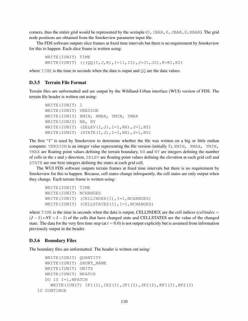
corners, thus the entire grid would be represented by the sextuple (0,IBAR,0,JBAR,0,KBAR). The gridnode positions are obtained from the Smokeview parameter input file.
The FDS software outputs slice frames at fixed time intervals but there is no requirement by Smokeviewfor this to happen. Each slice frame is written using:
WRITE(IUNIT) TIMEWRITE(IUNIT) (((QQ(I,J,K),I=11,I2),J=J1,J2),K=K1,K2)
where TIME is the time in seconds when the data is ouput and QQ are the data values.
D.3.5 Terrain File Format
Terrain files are unformatted and are output by the Wildland-Urban interface (WUI) version of FDS. Theterrain file header is written out using:
WRITE(IUNIT) 1WRITE(IUNIT) VERSIONWRITE(IUNIT) XMIN, XMAX, YMIN, YMAXWRITE(IUNIT) NX, NYWRITE(IUNIT) (ZELEV(I,J),I=1,NX),J=1,NY)WRITE(IUNIT) (STATE(I,J),I=1,NX),J=1,NY)
The first “1” is used by Smokeview to determine whether the file was written on a big or little endiancomputer. VERSION is an integer value representing the file version (initially 1), XMIN, XMAX, YMIN,YMAX are floating point values defining the terrain boundary, NX and NY are integers defining the numberof cells in the x and y direction, ZELEV are floating point values defining the elevation at each grid cell andSTATE are one byte integers defining the states at each grid cell.
The WUI FDS software outputs terrain frames at fixed time intervals but there is no requirement bySmokeview for this to happen. Because, cell states change infrequently, the cell states are only output whenthey change. Each terrain frame is written using:
WRITE(IUNIT) TIMEWRITE(IUNIT) NCHANGESWRITE(IUNIT) (CELLINDEX(I),I=1,NCHANGES)WRITE(IUNIT) (CELLSTATES(I),I=1,NCHANGES)
where TIME is the time in seconds when the data is output, CELLINDEX are the cell indices (cellindex =(J− 1) ∗NY + I− 1) of the cells that have changed state and CELLSTATES are the value of the changedstate. The data for the very first time step (at t = 0.0) is not output explicitly but is assumed from informationpreviously output in the header.
D.3.6 Boundary Files
The boundary files are unformatted. The header is written out using:
WRITE(IUNIT) QUANTITYWRITE(IUNIT) SHORT_NAMEWRITE(IUNIT) UNITSWRITE(IUNIT) NPATCHDO 10 I=1,NPATCH
WRITE(IUNIT) IP1(I),IP2(I),JP1(I),JP2(I),KP1(I),KP2(I)10 CONTINUE
110
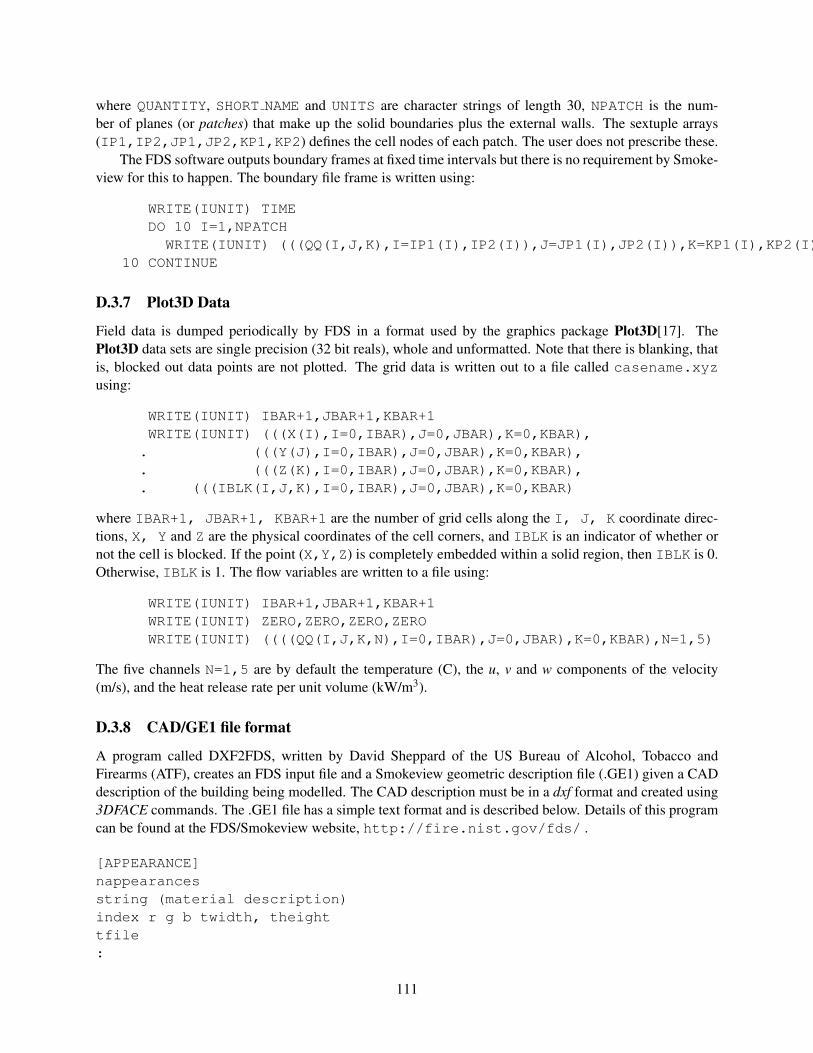
where QUANTITY, SHORT NAME and UNITS are character strings of length 30, NPATCH is the num-ber of planes (or patches) that make up the solid boundaries plus the external walls. The sextuple arrays(IP1,IP2,JP1,JP2,KP1,KP2) defines the cell nodes of each patch. The user does not prescribe these.
The FDS software outputs boundary frames at fixed time intervals but there is no requirement by Smoke-view for this to happen. The boundary file frame is written using:
WRITE(IUNIT) TIMEDO 10 I=1,NPATCH
WRITE(IUNIT) (((QQ(I,J,K),I=IP1(I),IP2(I)),J=JP1(I),JP2(I)),K=KP1(I),KP2(I))10 CONTINUE
D.3.7 Plot3D Data
Field data is dumped periodically by FDS in a format used by the graphics package Plot3D[17]. ThePlot3D data sets are single precision (32 bit reals), whole and unformatted. Note that there is blanking, thatis, blocked out data points are not plotted. The grid data is written out to a file called casename.xyzusing:
WRITE(IUNIT) IBAR+1,JBAR+1,KBAR+1WRITE(IUNIT) (((X(I),I=0,IBAR),J=0,JBAR),K=0,KBAR),
. (((Y(J),I=0,IBAR),J=0,JBAR),K=0,KBAR),
. (((Z(K),I=0,IBAR),J=0,JBAR),K=0,KBAR),
. (((IBLK(I,J,K),I=0,IBAR),J=0,JBAR),K=0,KBAR)
where IBAR+1, JBAR+1, KBAR+1 are the number of grid cells along the I, J, K coordinate direc-tions, X, Y and Z are the physical coordinates of the cell corners, and IBLK is an indicator of whether ornot the cell is blocked. If the point (X,Y,Z) is completely embedded within a solid region, then IBLK is 0.Otherwise, IBLK is 1. The flow variables are written to a file using:
WRITE(IUNIT) IBAR+1,JBAR+1,KBAR+1WRITE(IUNIT) ZERO,ZERO,ZERO,ZEROWRITE(IUNIT) ((((QQ(I,J,K,N),I=0,IBAR),J=0,JBAR),K=0,KBAR),N=1,5)
The five channels N=1,5 are by default the temperature (C), the u, v and w components of the velocity(m/s), and the heat release rate per unit volume (kW/m3).
D.3.8 CAD/GE1 file format
A program called DXF2FDS, written by David Sheppard of the US Bureau of Alcohol, Tobacco andFirearms (ATF), creates an FDS input file and a Smokeview geometric description file (.GE1) given a CADdescription of the building being modelled. The CAD description must be in a dxf format and created using3DFACE commands. The .GE1 file has a simple text format and is described below. Details of this programcan be found at the FDS/Smokeview website, http://fire.nist.gov/fds/ .
[APPEARANCE]nappearancesstring (material description)index r g b twidth, theighttfile:
111
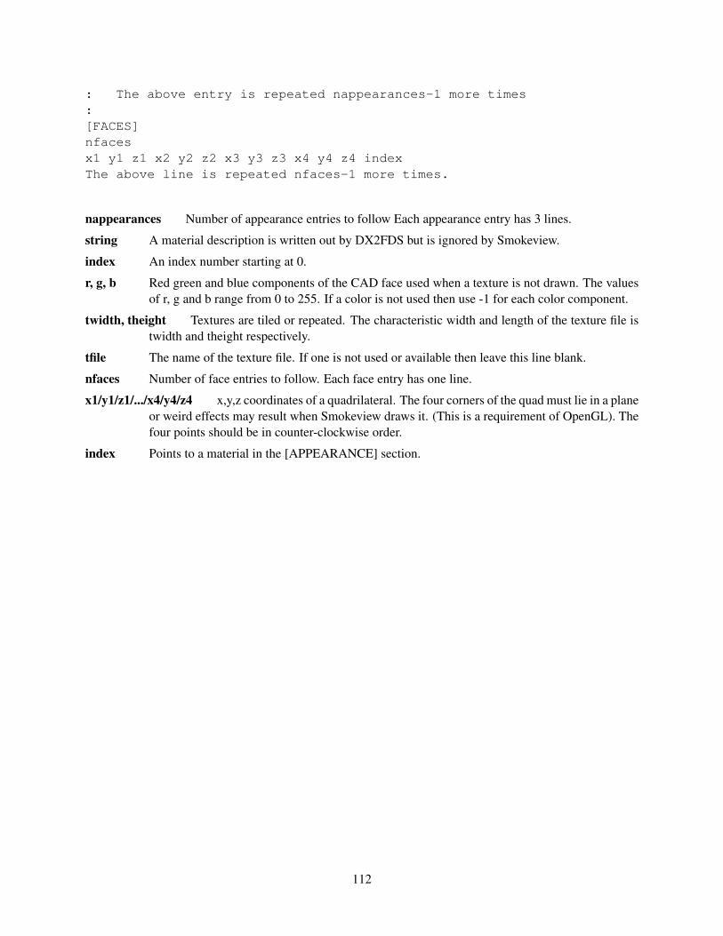
: The above entry is repeated nappearances-1 more times:[FACES]nfacesx1 y1 z1 x2 y2 z2 x3 y3 z3 x4 y4 z4 indexThe above line is repeated nfaces-1 more times.
nappearances Number of appearance entries to follow Each appearance entry has 3 lines.
string A material description is written out by DX2FDS but is ignored by Smokeview.
index An index number starting at 0.
r, g, b Red green and blue components of the CAD face used when a texture is not drawn. The valuesof r, g and b range from 0 to 255. If a color is not used then use -1 for each color component.
twidth, theight Textures are tiled or repeated. The characteristic width and length of the texture file istwidth and theight respectively.
tfile The name of the texture file. If one is not used or available then leave this line blank.
nfaces Number of face entries to follow. Each face entry has one line.
x1/y1/z1/.../x4/y4/z4 x,y,z coordinates of a quadrilateral. The four corners of the quad must lie in a planeor weird effects may result when Smokeview draws it. (This is a requirement of OpenGL). Thefour points should be in counter-clockwise order.
index Points to a material in the [APPEARANCE] section.
112

Appendix E
Frequently Asked Questions
This appendix contains a list of frequently asked questions concerning Smokeview.
E.1 Can I run Smokeview on other machines?
Smokeview is more complicated to compile on other platforms because it uses several freeware librariesthat need to be compiled and installed on that particular machine. We have compiled Smokeview on thePC, SGI (IRIX), and Red Hat Linux, but with the exception of the PC executable, there’s no guarantee thatsomething we compile on one of our machines is going to work on yours. Worse comes to worse, use a PCto visualize the output of a calculation run on your other machine.
E.2 Smokeview doesn’t look right on my computer. What’s wrong?
Some video cards do not use enough bits to represent the depth buffer. The depth buffer is used to determinewhen objects are hidden and therefore should not be drawn. A problem then can occur when the video cardreduces the number of depth buffer bits from 32 to 16 in order to speed up its performance (less data totransport). This results in straight lines or polygonal edges appearing to be scalloped. Often reducing theacceleration setting for the video card can eliminate this problem. To do this:
• click your mouse on the desktop to bring up the Display dialog box.
• click on the ”Advanced...” button
• Find the dialog panel that lets you select the ”Hardware acceleration”. Reduce the acceleration (re-booting if necessary) until the scalloping disappears.
If you have upgraded your PC recently, make sure you have loaded the latest drivers for your video card.
E.3 How do I make a movie of a Smokeview animation?
You make a movie of a Smokeview animation by converting the visualized scene into a series of PNG orJPEG files, one file for each time. More specifically:
• Set up Smokeview orienting the scene and loading the desired data files.
113

• Select the Options/Render menu and pick the desired frame rate. The more frames you include inthe animation, the smoother it will look. Of course more frames results in larger file sizes.
• Use a program such as the Antechinus Media Editor or Platypus Animator available at http://www.c-point.com
E.4 Smokeview is running much slower than I expected. What can I do?
A likely explanation is that your video drivers are not hardware accelerated for OpenGL. You need to down-load the latest drivers for your video card. You may also try playing around with the hardware acclerationsettings (see E.2).
E.5 I loaded a particle file but Smokeview is not displaying particles. Whatis wrong?
This is a bug in your video card. To see particles, reduce your hardware acceleration setting (see E.2).
E.6 Why do blockages not appear the way I defined them in my input file?( invisible blockages are visible, smooth blockages are not smooth etc )What is wrong?
Blockage appearance is controlled by the Show/Hide ¿ Geometry ¿ Blockages menu setting. Blockages willappear as defined in the input file if you set Defined in Input File under this menu. To set the behaviorto drawing blockages as defined in the input file, use the SHOWBLOCKS preference file keyword. TheSHOWBLOCKS keyword defined in the smokeview.ini preference file ( or the casename.ini preferencefile for your case ) may be set to 1 to cause Smokeview to display blockages as defined in the input file. Asalways, you may also create a preference file, after you have set Smokeview menu options to display scenesas desired.
114