www.SandV.com12 SOUND & VIBRATION/MARCH 2014

The use of single- and double-layer microphone arrays, both hand held as well as robot operated, has been greatly extended within the last decade. This article summarizes how a small double-layer array with typically 128 microphones can be used for interior cabin measurements for mapping various acoustical properties. There are four major applications. The first is general patch holography (or conformal mapping) of basic acoustical quantities like sound pressure, particle velocity and sound in-tensity. Additionally, sound quality (SQ) metrics for describing human annoyance like loudness, sharpness, fluctuation strength and roughness etc. can also be mapped. Other applications are: in-situ absorption measurements – for example, inside a car cabin; intensity component analysis (incident, scattered, radiated, net intensity etc. can be separated); and finally sound pressure contribution from various panels inside the cabin to the driver’s position. Some measurements are done in operational conditions, and some are reference laboratory measurements of typical fre-quency response functions.

Traditional near-field acoustic holography (NAH) was first intro-duced in the early 1980s,1,2 NAH allows one to obtain a complete model of the sound field in the vicinity of a sound source; that is, all sound field quantities (sound pressure, particle velocity, active and reactive intensity) can be calculated at any location based on pressure measurements on a planar surface in front of the sound source. In particular, the sound field can be mapped closer to the source than the measurement plane, which can provide very high spatial resolution of the source distribution. NAH was typi-cally implemented in the spatial frequency domain using a two-dimensional spatial Fourier transform.3 One of the drawbacks of the original formulation was that the measurement area should adequately cover the full source plus some “additional” area; so the basic hypothesis that practically all energy of the sound field radiated into the half-space passes through the measurement window was fulfilled. The upper frequency limit is given in that microphone spacing must be less than a half wavelength to avoid spatial aliasing. Practical measurements were performed using a sub-array and scan techniques. Reference transducers are needed to link the scan measurement together.4,5

Statistically optimized near-field acoustic holography (SONAH) became a new formulation of NAH, performing the plane-to-plane transformation directly in the spatial domain avoiding the use of spatial DFT and avoiding/eliminating windowing and leakage er-rors associated with FFT/DFT calculations. SONAH opens up the use of holography measurements with an array that is much smaller than the source − small hand-held arrays and still keeping errors at an acceptable level.6,7 SONAH also opens up the introduction of irregular array geometries that can be used for both holography measurements (low to medium frequencies) and beamforming (medium to high frequencies), covering the full frequency range.8

The first application of a small array was patch holography, where you just measure where it is relevant (for example around a door seal for sound leakage detection) rather than measuring around the whole vehicle. Today the use of a small array has been extended to several applications such as in-situ absorption measurement, intensity component analysis (incident, scattered, radiated, net intensity etc.) and panel contribution. Also, a more precise core holography algorithm similar to SONAH − the equiva-

lent-source method (ESM) for measuring curved surfaces has been developed recently (see Figure 1).9,10 This article gives an overview of the four applications, as well as the new ESM algorithm.

Equivalent Source MethodUsing ESM, the acoustic field is predicted directly by a mesh set

of weighted equivalent monopole sources mostly located inside the vibrating body, so the method is suitable for arbitrary source shapes (see Figure 1a). Here the requirement of having a model that can represent all contributions to the sound field in the test region is not fulfilled, but because of the short distance between the measurement area and reconstruction area, a good approximation for the local patch can be expected.

Furthermore, if the mesh is arranged so that it surrounds a two-layer microphone array and with a part of the mesh surface coinciding with the patch of interest, then the requirement of having a model that can represent all contributions to the sound field in the test region is fulfilled for local sound field modeling (see Figure 1b). Global sound field modeling is then obtained by a series of patch measurements. In addition, using an array with two layers, sources are allowed behind the array.

The major difference between SONAH and ESM from an applica-tion point of view is that ESM handles arbitrary shaped sources and curved surfaces better than SONAH (see Figure 2). SONAH uses a sound field model in terms of plane propagating and evanescent waves, while ESM uses a source model. So where ESM relies on the definition of a sufficient set of monopole sources, this is not the case for SONAH.

InstrumentationThe measurement system is detailed in Reference 11. The sound

field measuring part consists of a 128-channel, hand-held micro-phone array (Figure 3a), a 132-channel, LAN-XI front end (Figure 3b), a positioning system integrated into the array frame and a PC with dedicated software.

Using Hand-Held Arrays for Automotive NVH MeasurementsSvend Gade, Jesper Gomes, and Jørgen Hald, Brüel & Kjær, Nærum, Denmark

Figure 1. (a) ESM modeling using single-layer array; (b) ESM modeling us-ing double-layer array.

(a) Single-layer array (b) Double-layer array

Equivalent Modeling reflections sources or rear sources

Figure 2. (a) Valid region of SONAH algorithm; (b) valid region of ESM algorithm.

Based on a paper presented at Inter-Noise 2013, Innsbruck, Austria, Sep-tember 15-18 2013.

www.SandV.com SOUND & VIBRATION/MARCH 2014 13

The array shown in figure 3a has 8¥8 microphones mounted in two layers, resulting in a total of 128 microphones. An array of for instance 6¥6¥2=72 microphones can also be used. The micro-phones are spaced 25 mm apart (distances from 25 to 50 mm are available) in both directions with a spacing of 31 mm between the two layers. This results in an upper frequency limit for the array of 5 kHz (spatial sampling limit). Due to corrections for phase response stored in transducer electronic data sheet (TEDS) information, the array performs to frequencies very well below 200 Hz. In general TEDS corrections will improve the available dynamic range over a broad frequency range.13,14 The array is connected to the front end via a single cable as shown in Figure 3b.

A 3D Creator system consisting of an optical sensor unit, a digi-tizer control unit, a wireless hand-held probe, and a wired dynamic reference frame enables precise three-dimensional measurement of array position in real time as well as capturing of the surface geometry of the device under test.

Applications of a Hand-Held ArrayToday, four major applications of a small hand held array exist:

patch holography, absorption measurements, intensity component analysis and panel contribution.

Patch Holography/Conformal Mapping. This is the fundamental application of a hand-held microphone array. First a geometry sur-face model can be created by the positioning system or imported from a CAD or mesh model. Actual measurements are done with the small, double-layer array (DLA) for interior noise measure-ments, diffuse sound fields or single layer array (SLA) for exterior noise measurements in semi-anechoic sound fields. The array is mounted on a handle with a built-in 3D position measurement system (Figure 3a).

The system continuously determines the positions of the array microphones relative to some user-defined coordinate system. To map the sound field on a surface larger than the array, patch measurements are made with the array in neighboring (preferably overlapping) positions over the surface. In each array patch posi-tion, acoustic and position data belonging together are recorded. Patch positions already visited/measured are displayed in a 3D

view along with the real-time updated current position of the array. Also shown in the 3D view is a surface model of the test object. This way the user is guided in covering the surface area with sufficient array patch positions to obtain a reliable surface mapping result. To minimize errors in the patch holography calculations, a very small measurement distance is recommended, typically equal to half of the microphone grid spacing. If this is not possible, then patches with significant overlap should be used, avoiding the need to perform calculations near the boundaries of the array areas.

The procedure is depicted in Figure 4 using a simple loudspeaker (boombox) example. Figure 4a shows the individual six measure-ment patches (with no or little overlap), while Figure 4b shows the sound intensity results of patch holography/conformal mapping. Typical sound field quantities like sound pressure, particle veloc-ity and sound intensity can be mapped. Optional sound quality metrics for describing human annoyance like loudness, sharpness, fluctuation strength and roughness etc. can also be mapped.

In Situ Absorption Measurements. The double-layer array in combination with holography calculations yields the three in-tensity components: the net/total intensity, positive (from front direction) and negative (from rear direction) intensity:

When estimating surface absorption, a number of loudspeakers

are distributed in the cabin interior and driven by uncorrelated noise sources to create a distributed and (close-to) diffuse excita-tion field. The net intensity is also the sum of the radiated and absorbed intensity. So in this simple case (Irad = 0) the absorption coefficient, a can be calculated from:

Figure 3. (a) Double-layer array with 8 ¥ 8 ¥ 2 microphones; (b) 132-channel front end with single cable connection to array.

(1)I I I I I Itot net front rear rad abs( ) = + = +

Figure 4. (a) Six measurement patches; (b) patch holography/conformal mapping results.

www.SandV.com14 SOUND & VIBRATION/MARCH 2014

That is, a can be calculated when Itot and Irear are known. 11,15

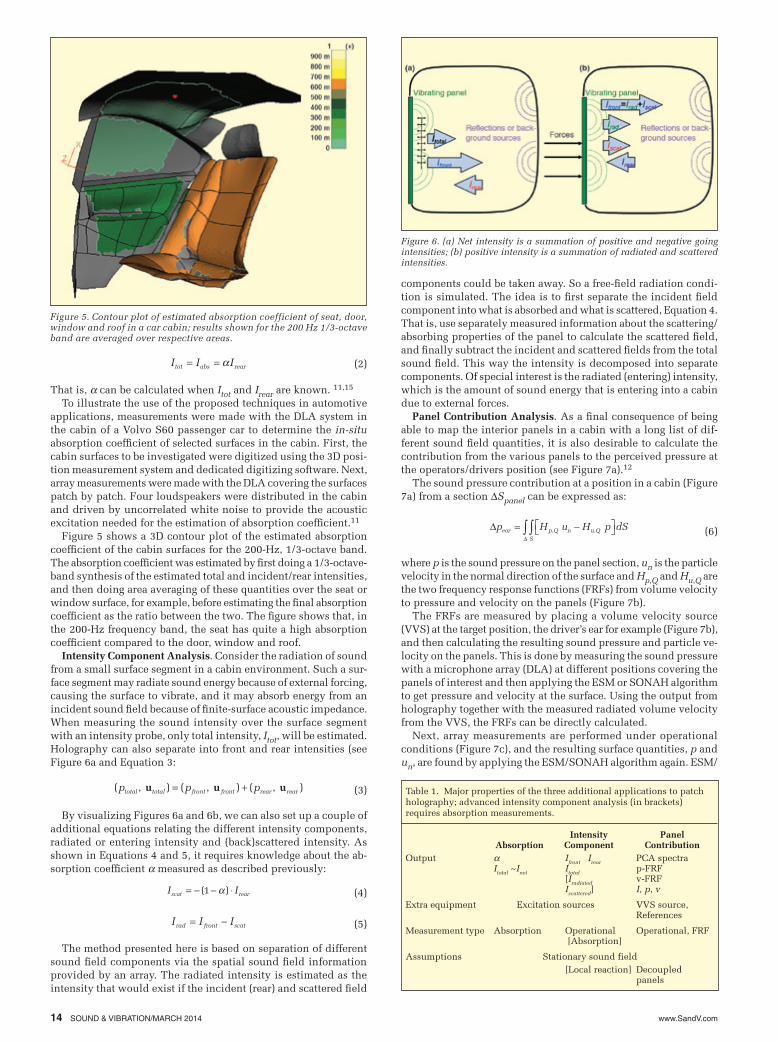
To illustrate the use of the proposed techniques in automotive applications, measurements were made with the DLA system in the cabin of a Volvo S60 passenger car to determine the in-situ absorption coefficient of selected surfaces in the cabin. First, the cabin surfaces to be investigated were digitized using the 3D posi-tion measurement system and dedicated digitizing software. Next, array measurements were made with the DLA covering the surfaces patch by patch. Four loudspeakers were distributed in the cabin and driven by uncorrelated white noise to provide the acoustic excitation needed for the estimation of absorption coefficient.11

Figure 5 shows a 3D contour plot of the estimated absorption coefficient of the cabin surfaces for the 200-Hz, 1/3-octave band. The absorption coefficient was estimated by first doing a 1/3-octave-band synthesis of the estimated total and incident/rear intensities, and then doing area averaging of these quantities over the seat or window surface, for example, before estimating the final absorption coefficient as the ratio between the two. The figure shows that, in the 200-Hz frequency band, the seat has quite a high absorption coefficient compared to the door, window and roof.

Intensity Component Analysis. Consider the radiation of sound from a small surface segment in a cabin environment. Such a sur-face segment may radiate sound energy because of external forcing, causing the surface to vibrate, and it may absorb energy from an incident sound field because of finite-surface acoustic impedance. When measuring the sound intensity over the surface segment with an intensity probe, only total intensity, Itot, will be estimated. Holography can also separate into front and rear intensities (see Figure 6a and Equation 3:

By visualizing Figures 6a and 6b, we can also set up a couple of additional equations relating the different intensity components, radiated or entering intensity and (back)scattered intensity. As shown in Equations 4 and 5, it requires knowledge about the ab-sorption coefficient a measured as described previously:

The method presented here is based on separation of different sound field components via the spatial sound field information provided by an array. The radiated intensity is estimated as the intensity that would exist if the incident (rear) and scattered field

Figure 5. Contour plot of estimated absorption coefficient of seat, door, window and roof in a car cabin; results shown for the 200 Hz 1/3-octave band are averaged over respective areas.

Figure 6. (a) Net intensity is a summation of positive and negative going intensities; (b) positive intensity is a summation of radiated and scattered intensities.

components could be taken away. So a free-field radiation condi-tion is simulated. The idea is to first separate the incident field component into what is absorbed and what is scattered, Equation 4. That is, use separately measured information about the scattering/absorbing properties of the panel to calculate the scattered field, and finally subtract the incident and scattered fields from the total sound field. This way the intensity is decomposed into separate components. Of special interest is the radiated (entering) intensity, which is the amount of sound energy that is entering into a cabin due to external forces.

Panel Contribution Analysis. As a final consequence of being able to map the interior panels in a cabin with a long list of dif-ferent sound field quantities, it is also desirable to calculate the contribution from the various panels to the perceived pressure at the operators/drivers position (see Figure 7a).12

The sound pressure contribution at a position in a cabin (Figure 7a) from a section DSpanel can be expressed as:

where p is the sound pressure on the panel section, un is the particle velocity in the normal direction of the surface and Hp,Q and Hu,Q are the two frequency response functions (FRFs) from volume velocity to pressure and velocity on the panels (Figure 7b).

The FRFs are measured by placing a volume velocity source (VVS) at the target position, the driver’s ear for example (Figure 7b), and then calculating the resulting sound pressure and particle ve-locity on the panels. This is done by measuring the sound pressure with a microphone array (DLA) at different positions covering the panels of interest and then applying the ESM or SONAH algorithm to get pressure and velocity at the surface. Using the output from holography together with the measured radiated volume velocity from the VVS, the FRFs can be directly calculated.

Next, array measurements are performed under operational conditions (Figure 7c), and the resulting surface quantities, p and un, are found by applying the ESM/SONAH algorithm again. ESM/

(2)I I Itot abs rear= = a

(3)( , ) ( , ) ( , )p p ptotal total front front rear rear u u u= +

(4)I Iscat rear= - - ◊( )1 a

(5)I I Irad front scat= -

(6)DD

p H u H p dSear p Q n u QS

= -ÈÎ ˘̊ÚÚ , ,

Table 1. Major properties of the three additional applications to patch holography; advanced intensity component analysis (in brackets) requires absorption measurements.

Intensity Panel Absorption Component ContributionOutput a Ifront Irear PCA spectra Itotal ~Inet Itotal p-FRF [Iradiated v-FRF Iscattered] I, p, v

Extra equipment Excitation sources VVS source, References

Measurement type Absorption Operational Operational, FRF [Absorption]

Assumptions Stationary sound field [Local reaction] Decoupled panels

www.SandV.com SOUND & VIBRATION/MARCH 2014 15

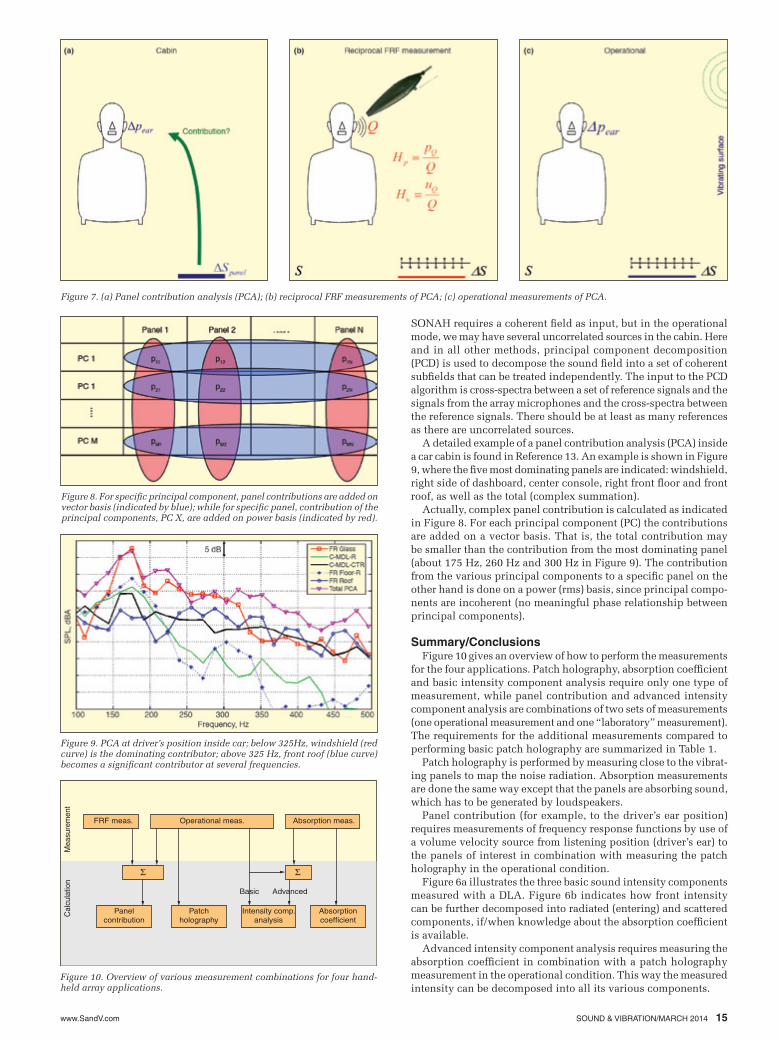
Figure 7. (a) Panel contribution analysis (PCA); (b) reciprocal FRF measurements of PCA; (c) operational measurements of PCA.

Figure 9. PCA at driver’s position inside car; below 325Hz, windshield (red curve) is the dominating contributor; above 325 Hz, front roof (blue curve) becomes a significant contributor at several frequencies.

Figure 8. For specific principal component, panel contributions are added on vector basis (indicated by blue); while for specific panel, contribution of the principal components, PC X, are added on power basis (indicated by red).

Figure 10. Overview of various measurement combinations for four hand-held array applications.

SONAH requires a coherent field as input, but in the operational mode, we may have several uncorrelated sources in the cabin. Here and in all other methods, principal component decomposition (PCD) is used to decompose the sound field into a set of coherent subfields that can be treated independently. The input to the PCD algorithm is cross-spectra between a set of reference signals and the signals from the array microphones and the cross-spectra between the reference signals. There should be at least as many references as there are uncorrelated sources.

A detailed example of a panel contribution analysis (PCA) inside a car cabin is found in Reference 13. An example is shown in Figure 9, where the five most dominating panels are indicated: windshield, right side of dashboard, center console, right front floor and front roof, as well as the total (complex summation).

Actually, complex panel contribution is calculated as indicated in Figure 8. For each principal component (PC) the contributions are added on a vector basis. That is, the total contribution may be smaller than the contribution from the most dominating panel (about 175 Hz, 260 Hz and 300 Hz in Figure 9). The contribution from the various principal components to a specific panel on the other hand is done on a power (rms) basis, since principal compo-nents are incoherent (no meaningful phase relationship between principal components).

Summary/ConclusionsFigure 10 gives an overview of how to perform the measurements

for the four applications. Patch holography, absorption coefficient and basic intensity component analysis require only one type of measurement, while panel contribution and advanced intensity component analysis are combinations of two sets of measurements (one operational measurement and one “laboratory” measurement). The requirements for the additional measurements compared to performing basic patch holography are summarized in Table 1.

Patch holography is performed by measuring close to the vibrat-ing panels to map the noise radiation. Absorption measurements are done the same way except that the panels are absorbing sound, which has to be generated by loudspeakers.

Panel contribution (for example, to the driver’s ear position) requires measurements of frequency response functions by use of a volume velocity source from listening position (driver’s ear) to the panels of interest in combination with measuring the patch holography in the operational condition.

Figure 6a illustrates the three basic sound intensity components measured with a DLA. Figure 6b indicates how front intensity can be further decomposed into radiated (entering) and scattered components, if/when knowledge about the absorption coefficient is available.

Advanced intensity component analysis requires measuring the absorption coefficient in combination with a patch holography measurement in the operational condition. This way the measured intensity can be decomposed into all its various components.

FRF meas. Operational meas. Absorption meas.

Panelcontribution

Intensity comp.analysis

Absorptioncoefficient

Patchholography

Cal

cula

tion

Mea

sure

men

t

Basic Advanced

S S

www.SandV.com16 SOUND & VIBRATION/MARCH 2014

References 1. J. D. Maynard, E. G. Williams and Y. Lee, “Near-field Acoustic Hologra-

phy I: Theory of Generalized Holography and the Development of NAH,” Journal Acoustical Society America, 78(4), pp. 1395-1413, October 1985.

2. Earl G. Williams, Fourier Acoustics, Sound Radiation and Near-field Acoustical Holography, Acedemic Press, London, Book 306, pp. 1999.

3. W. A. Veronesi and J. D. Maynard, “Near-field Acoustic Holography (NAH) II: Holographic Reconstruction Algorithms and Computer Imple-mentation,” Journal Acoustical Society America, 81(5), pp. 1307-1322, May 1987.

4. J. Hald, “STSF –A Unique Technique for Scan Based Near-Field Acoustic Holography Without Restrictions on Coherence,” Brüel & Kjær Technical Review No. 1, 1989.

5. K. B. Ginn and J. Hald, “STSF – Practical Instrumentation and applica-tions,” Brüel & Kjær Technical Review No. 2, 1989.

6. R. Steiner and J. Hald, “Near-field Acoustical Holography Without the Errors and Limitations Caused by the Use of Spatial DFT,” International Journal of Acoustics and Vibration, 6 (2), June 2001.

7. J. Hald, “Planar Near-field Acoustical Holography with Arrays Smaller Than the Sound Source”, Proceedings of ICA, 2001.

8. J. Hald, “Combining NAH and Beamforming Using the Same Array,” Brüel & Kjær Technical Review No. 1, 2005. The author can be reached at: svend.gade@bksv.com.

9. M. Pinho and J. Arruda, “On the Use of the Equivalent Source Method for Near-field Acoustic Holography,” ABCM Symposium Series in Me-chatronics, Vol. 1- pp. 590-599, 2004.

10. J. Gomes, “Patch Holography Using a Double Layer Microphone Array,” Proceedings of Inter-noise, 2007.

11. J. Mørkholt, J. Hald and S. Gade, “Measurement of Absorption Coeffi-cient, Radiated and Absorbed Intensity on the Panels of a Vehicle Cabin using a Dual-Layer Array with Integrated Position Measurements,” JSAE Paper 20105022, 2010.

12. J. Hald, “Panel Contribution Analysis Using a Volume Velocity Source and a Double-Layer Array with SONAH Algorithm,” Proceedings of Inter-noise, 2006.

13. J. Gomes, M. Wada, Y. Fukuju, Y. Ishii, J. Hald, T. Satoh, “In-Cabin Array-Based Panel Contribution Analysis with a Vehicle Running on a Dyno,” JSAE Paper 20115359, 2011

14. J. Hald, “Performance Investigation of the Dual-Layer Array at Low Frequencies,” Brüel & Kjær Technical Review No. 1, 2011.

15. J. Hald, J. Mørkholt, P. Hardy, D. Trentin, M. Bach-Andersen and G. Keith, “Array Based Measurement of Radiated and Absorbed Sound Intensity Components,” Proceedings of EuroNoise, 2008.