using interest rate derivative prices to estimate … · the world to adopt unprecedented policy...
TRANSCRIPT

Working Paper 04/2010 24 June 2010
USING INTEREST RATE DERIVATIVE PRICES TO ESTIMATE LIBOR-OIS SPREAD DYNAMICS AND
SYSTEMIC FUNDING LIQUIDITY SHOCK PROBABILITIES
Prepared by Cho-Hoi Hui and Tsz-Kin Chung Research Department
Chi-fai Lo Physics Department, The Chinese University of Hong Kong
Abstract
Following the bankruptcy of Lehman Brothers in mid-September 2008, there were severe disruptions in international money markets and banks reportedly faced severe liquidity shocks, in particular US-dollar funding shortages, prompting central banks around the world to adopt unprecedented policy measures to supply funds to the banks. The turbulence also spilled over to the money market in Hong Kong. A better understanding of the forward-looking information content about funding liquidity risk in the prices of interest-rate derivative instruments is therefore necessary to gauge pressures on systemic liquidity. Using the market prices of the US-dollar LIBOR-overnight index swap (OIS) spread, we estimate the probability of the systemic funding liquidity shock during the crisis period, which deviated from zero on 18 September 2008 to 12%. This provided an early warning signal of the systemic liquidity shock on 29 September 2008 when the interbank market was paralysed and the Federal Reserve authorised a US$330 billion expansion of swap lines with other central banks. JEL classification: F31;G13 Keywords: Sub-prime crisis; funding liquidity shocks; LIBOR-OIS spread; first-passage-time probability Authors’ E-Mail Addresses: [email protected]; [email protected]; [email protected]
The views and analysis expressed in this paper are those of the authors, and do not necessarily represent the views of the Hong Kong Monetary Authority.

- 2 -
EXECUTIVE SUMMARY • Following the bankruptcy of Lehman Brothers in mid-September 2008, uncertainty
about losses incurred in banks increased their liquidity needs as well as their reluctance to lend to each other in money markets. There were severe disruptions in international money markets and banks reportedly faced severe liquidity shocks, in particular US-dollar funding shortages. Reflecting these and possibly other factors, interbank short-term interest rates surged substantially after the Lehman failure, and then persisted at high levels, prompting central banks around the world to adopt unprecedented policy measures to supply funds to the banks.
• The global turbulence also spilled over to the money market in Hong Kong.
The HKMA and the Government therefore announced a series of measures to help contain the global risks from spilling over to the domestic banking system. In particular, the five temporary measures provided additional longer-term funding to banks against a wider range of collateral at a potentially lower interest-rate cost.
• A better understanding of the forward-looking information content about funding
liquidity risk in prices of interest-rate derivative instruments is necessary to improve the measurement of system-wide liquidity risk. Using the market prices, this paper derives the dynamics of the US-dollar LIBOR-overnight index swap (OIS) spread, which are considered as the funding liquidity risk premium and have been widely used by central banks to gauge funding liquidity conditions. We find that the dynamics contained significant probability of extreme price movements of the LIBOR-OIS spread during the crisis of 2008 reflecting deepened uncertainty about the funding liquidity risk.
• The dynamics provide information to estimate the probability of the systemic funding
liquidity shock during the crisis period. The probability deviated from zero on 18 September 2008 to 12%, which provided an early warning signal of the systemic liquidity shock on 29 September 2008 when the interbank market was paralysed and the Federal Reserve authorised a US$330 billion expansion of swap lines with other central banks.
• The information content about funding liquidity risk in prices of interest-rate
derivative instruments could help the financial system be more prepared for liquidity shocks. The forward-looking probabilities of funding liquidity shocks derived in this paper could serve as a basis for the development of a set of potential early warning indicators, which could be used to indicate whether pressures on systemic liquidity are building up.
- 3 -
I. INTRODUCTION The sub-prime crisis emerged in the United States in mid-2007 and spilled
over to other economies. From mid-2007 to mid-2008, the spillovers were relatively modest. Following the bankruptcy of Lehman Brothers in mid-September 2008, developments took a dramatic turn. One channel for spillovers was severe disruptions in international money markets, especially the US-dollar denominated money markets. Uncertainty about losses incurred in banks increased their liquidity needs as well as their reluctance to lend to each other in money markets. Banks reportedly faced severe liquidity shocks in particular US-dollar funding shortages. Reflecting these and possibly other factors, interbank short-term interest rates surged substantially after the Lehman failure, and then persisted at high levels, prompting central banks around the world to adopt unprecedented policy measures to supply funds to the banks (see McGuire and von Peter (2009)). Among these measures, the Federal Reserve established unlimited US-dollar swap lines with foreign central banks on 13 October 2008.1
Since the emergence of the crisis in August 2007, risk premiums in
short-term money market rates, as represented by the spreads between LIBOR and overnight index swap (OIS) rates, increased significantly in the US dollar. An OIS is an interest-rate swap in which the floating leg is linked to an index of daily overnight rates. The two parties agree to exchange at maturity, on an agreed notional amount, the difference between interest rate accrued at the agreed fixed rate and interest accrued at the floating index rate over the life of the swap. The fixed rate is a proxy for expected future overnight interest rates. As overnight interest rates generally bear lower credit and liquidity risks, the credit risk and liquidity risk premiums contained in the OIS rates should be small. The OIS rates are typically thought to provide the best estimates of the mean expectation for central banks’ policy rates. Therefore, the spread of LIBOR relative to the OIS rate generally reflects the funding liquidity risks in the interbank market.2,3 1 Sizes of the US-dollar swap lines between the Federal Reserve and the Bank of England (BoE), the
European Central Bank (ECB) and the Swiss National Bank (SNB) had increased to accommodate the demand for whatever amount of US-dollar funding. A timeline of events and policy actions during the financial crisis is documented by the Federal Reserve Bank of St. Louis at http://timeline.stlouisfed.org/.
2 The LIBOR-OIS spread is generally viewed as reflecting two types of risk in relation to funding liquidity shocks. The first is the different interbank funding costs (the liquidity premiums paid by banks) of term lending (say three-month) and overnight lending rolled over for three months. A second component of the spreads stems from counterparty default risk. Schwarz (2009) finds that both credit and liquidity effects are important in explaining the widening of LIBOR-OIS spreads, but that market liquidity explains a greater share. This finding is consistent with that in McAndrews et al. (2008) who find that there is a substantial and time-varying liquidity component in LIBOR-OIS spreads. Michaud and Upper (2008) also find a significant role for liquidity in explaining money market spreads. While Taylor and Williams (2009) find a much smaller role for liquidity in LIBOR-OIS spreads, they argue that LIBOR can be pushed up as the lender demands compensation for taking on default risk due to poor market liquidity, or because of other factors, especially at times of market stress.
3 The LIBOR-OIS spread has been widely used by market participants and central banks to gauge funding liquidity conditions. See for example, page 32 in the BoE Financial Stability Report (June 2009, Issue No. 25) and page 38 in the IMF Global Financial Stability Report (Responding to the Financial Crisis and Measuring Systemic Risks, April 2009).

- 4 -
Figure 1 shows that the US-dollar one-month LIBOR-OIS spread – the premium of providing funding demanded by dollar lenders in the interbank market. As can be seen, before the summer of 2007 it oscillated around six basis points but after that started to follow an upward trend.4 Around the beginning of September 2008, it fluctuated wildly.
Figure 1: 1-month LIBOR-OIS spread and 1-month forward 1-month LIBOR-OIS spread
0
50
100
150
200
250
300
350
400
Jan-07 Apr-07 Jul-07 Oct-07 Jan-08 Apr-08 Jul-08 Oct-08
1-month spotLIBOR-OIS spread
1m2m forwardLIBOR-OIS spread
LIBOR-OIS spread (bps)
A better understanding of the information content about funding liquidity
risk in prices of interest-rate derivative instruments is necessary to improve the measurement of system-wide liquidity risk. This could potentially help the financial system be more prepared for liquidity shocks. The development of forward-looking measures of system-wide liquidity risk could serve as a basis for the development of a set of potential early warning indicators to show whether pressures on systemic liquidity are building up. This paper uses the forward-rate contracts of OIS and LIBOR to derive the term structure of the LIBOR-OIS spread as a measure of funding liquidity risk and the interest-rate cap prices (options refer to LIBOR) as the sources of market information for estimating the probability of liquidity shocks. Option markets have the desirable property of being forward-looking in nature and thus are a useful source of information for gauging market sentiment about future values of financial assets. Options, whose payoff depends on a limited range of the expected asset prices, offer broader information about market expectations than the forward asset prices. The entire risk neutral probability density function (PDF) of the asset price can be inferred from option prices. As options on both OIS rate and LIBOR-OIS spread were not available before the crisis, this paper estimates 4 BNP Paribas froze redemptions for three of its investment funds on 9 August 2007. This marked the
inception of the crisis.
- 5 -
the term structures and dynamics of the OIS rate and LIBOR-OIS spread based on the information on LIBOR options and by assuming the dynamics of the rates governed by the Cox–Ingersoll–Ross (CIR) model.5 The dynamics of the LIBOR-OIS spread, which are considered as the funding risk premium of LIBOR, are thus separated explicitly from the dynamics of LIBOR based on the information in the market prices. The PDFs for OIS rate and LIBOR-OIS spread are then constructed from their corresponding dynamics.
Using the dynamics and the term structure of the LIBOR-OIS spread, the
probability of systemic funding liquidity shocks is estimated using a first-passage-time (FPT) approach, which is a path-dependent contingent-claims approach. Path dependency is an intrinsic characteristic of systemic liquidity risk because a shortage of funding can be triggered by an important economic-political event (for example the failure of Lehman Brothers) during a time horizon under assessment. This means that a systemic liquidity shock could occur whenever the underlying measure (i.e. the LIBOR-OIS spread) breaches a pre-specified boundary during the time horizon of risk assessment. The probability estimated under the path-dependent approach takes into account the risk of the underlying measure passing through the boundary during some time interval. Conversely, the risk measurement of the path-independent approach depends on the measure only at the end of some time interval, and not on the particular path, so that the LIBOR-OIS spread is otherwise free to move to any level relative to the boundary. It therefore underestimates the risk by an amount equal to the probability of breaching the boundary during some time intervals.
The FPT approach has been applied to assessing risks in other areas of
financial economics. The nature of measurements of risks and their associated probabilities is common in their applications of the FPT approach, where the risk of a system (e.g. an exchange rate system) and an entity is governed by the dynamics of the underlying measure and measured by the associated probability of breaching a critical boundary. For example, the FPT approach has been used for estimating probability of corporate default in the Merton-type credit risk models.6 Because the original model in Merton (1974) has a weakness that default only occurs at the end of a time horizon (i.e. ignoring the possibility of early default), the model has since been generalised using the FPT approach to allow occurrence of default during a time horizon if a firm’s asset value hits a pre-specified default boundary. 7 Brockman and Turtle (2003) provide empirical evidence that path dependency is an intrinsic and fundamental characteristic of corporate securities because equity can be knocked out whenever a legally binding
5 Three-month US dollar overnight index swap options were launched by the CME Group Exchanges on
24 November 2008 but no daily volume has been reported so far. 6 Merton (1974) is the pioneer in the development of the structural models for credit risk of firms using a
contingent-claims framework. Default risk is equivalent to a European put option (i.e. path independent) on a firm’s asset value and the firm’s liability is the option strike.
7 Jarrow and Protter (2004) summarise the mathematical framework of these generalised credit risk models (e.g. in Black and Cox (1976)) in which default probabilities are estimated by the FPT approach.

- 6 -
boundary is breached. In the context of assessing realignment risk of a target-zone exchange rate regime, Hui and Lo (2009) find that path-dependency based on the FPT approach was quantitatively significant and provided more forward-looking assessment on the risk, compared with the path-independent approach, using information in the currency option prices of the British pound during the ERM crisis of 1992.8
In the following section, we discuss the information contents of the prices
of interest-rate forward contracts and options during the crisis. We construct the PDFs for the US-dollar OIS rates and LIBOR-OIS spreads in Section III. The estimations of systemic funding liquidity shocks using the FPT approach based on the market data during the crisis are presented in Section IV. The final section summarises the findings.
II. INFORMATION CONTENT IN FORWARD RATES AND INTEREST RATE OPTIONS
A forward-rate agreement (FRA) is a forward contract where the parties agree that a certain interest rate will apply to a certain principal during a specific period. An FRA uses the corresponding LIBOR as the benchmark and is generally settled in cash at the beginning of the specific period.9 Financial institutions or corporations may enter FRA contracts to lock-in the cost of funds for unsecured borrowing or the interest paid for floating-rate loans. Using the FRA rate, we can derive the forward LIBOR-OIS spread by subtracting the corresponding forward-starting OIS rate with the same contract period. Figure 1 shows the one-month forward and spot one-month LIBOR-OIS spreads. As can be seen, the forward spread moved in a different pattern with the spot LIBOR-OIS spread during certain periods.10 This indicates that the forward spread contains information different from that contained in the spot spread, probably about the future movements of the LIBOR-OIS spread.
8 The estimated realignment probabilities under the path-independent approach are defined as the
likelihood that the spot pound exchange rate is below the lower band (i.e. the lower fluctuation limit) at the end of a specified time horizon. Therefore, the estimation is independent of the path of the exchange rate within the time horizon. Such a path-independent approach has been used in estimating realignment risk in Campa and Chang (1996), Malz (1996), Mizrach (1996) and Söderlind (2000).
9 The agreed rate in an FRA should therefore always equal the forward rate at the time the contract is initiated. As there is no principal payment in an FRA contract, the credit and liquidity risks are very small. The loss due to default of the counterparty in the contract which is the potential mark-to-market profit is very small compared with an interbank loan. Hui and Chung (2009) examine the pricing anomalies in the interest-rate markets during the crisis period and find that the LIBOR curve contains a significant credit and liquidity premium over the equivalent FRA-implied curve.
10 Market data used in this paper are obtained from Bloomberg.
- 7 -
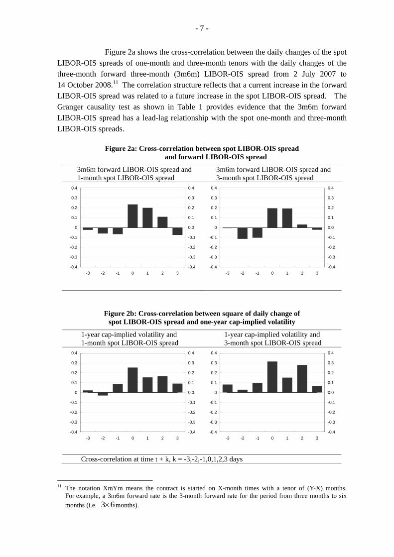
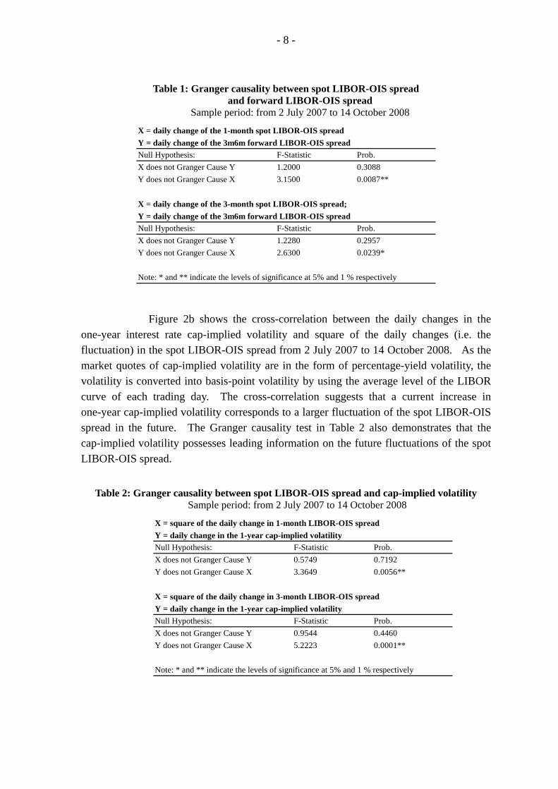
Figure 2a shows the cross-correlation between the daily changes of the spot LIBOR-OIS spreads of one-month and three-month tenors with the daily changes of the three-month forward three-month (3m6m) LIBOR-OIS spread from 2 July 2007 to 14 October 2008.11 The correlation structure reflects that a current increase in the forward LIBOR-OIS spread was related to a future increase in the spot LIBOR-OIS spread. The Granger causality test as shown in Table 1 provides evidence that the 3m6m forward LIBOR-OIS spread has a lead-lag relationship with the spot one-month and three-month LIBOR-OIS spreads.
Figure 2a: Cross-correlation between spot LIBOR-OIS spread and forward LIBOR-OIS spread
3m6m forward LIBOR-OIS spread and 1-month spot LIBOR-OIS spread
3m6m forward LIBOR-OIS spread and 3-month spot LIBOR-OIS spread
-0.4
-0.3
-0.2
-0.1
0
0.1
0.2
0.3
0.4
-3 -2 -1 0 1 2 3-0.4
-0.3
-0.2
-0.1
0.0
0.1
0.2
0.3
0.4
-0.4
-0.3
-0.2
-0.1
0
0.1
0.2
0.3
0.4
-3 -2 -1 0 1 2 3-0.4
-0.3
-0.2
-0.1
0.0
0.1
0.2
0.3
0.4
Figure 2b: Cross-correlation between square of daily change of spot LIBOR-OIS spread and one-year cap-implied volatility
1-year cap-implied volatility and 1-month spot LIBOR-OIS spread
1-year cap-implied volatility and 3-month spot LIBOR-OIS spread
-0.4
-0.3
-0.2
-0.1
0
0.1
0.2
0.3
0.4
-3 -2 -1 0 1 2 3-0.4
-0.3
-0.2
-0.1
0.0
0.1
0.2
0.3
0.4
-0.4
-0.3
-0.2
-0.1
0
0.1
0.2
0.3
0.4
-3 -2 -1 0 1 2 3-0.4
-0.3
-0.2
-0.1
0.0
0.1
0.2
0.3
0.4
Cross-correlation at time t + k, k = -3,-2,-1,0,1,2,3 days
11 The notation XmYm means the contract is started on X-month times with a tenor of (Y-X) months.
For example, a 3m6m forward rate is the 3-month forward rate for the period from three months to six months (i.e. 63× months).
- 8 -
Table 1: Granger causality between spot LIBOR-OIS spread
and forward LIBOR-OIS spread Sample period: from 2 July 2007 to 14 October 2008
X = daily change of the 1-month spot LIBOR-OIS spreadY = daily change of the 3m6m forward LIBOR-OIS spreadNull Hypothesis: F-Statistic Prob.X does not Granger Cause Y 1.2000 0.3088Y does not Granger Cause X 3.1500 0.0087**
X = daily change of the 3-month spot LIBOR-OIS spread; Y = daily change of the 3m6m forward LIBOR-OIS spreadNull Hypothesis: F-Statistic Prob.X does not Granger Cause Y 1.2280 0.2957Y does not Granger Cause X 2.6300 0.0239*
Note: * and ** indicate the levels of significance at 5% and 1 % respectively
Figure 2b shows the cross-correlation between the daily changes in the
one-year interest rate cap-implied volatility and square of the daily changes (i.e. the fluctuation) in the spot LIBOR-OIS spread from 2 July 2007 to 14 October 2008. As the market quotes of cap-implied volatility are in the form of percentage-yield volatility, the volatility is converted into basis-point volatility by using the average level of the LIBOR curve of each trading day. The cross-correlation suggests that a current increase in one-year cap-implied volatility corresponds to a larger fluctuation of the spot LIBOR-OIS spread in the future. The Granger causality test in Table 2 also demonstrates that the cap-implied volatility possesses leading information on the future fluctuations of the spot LIBOR-OIS spread.
Table 2: Granger causality between spot LIBOR-OIS spread and cap-implied volatility Sample period: from 2 July 2007 to 14 October 2008
X = square of the daily change in 1-month LIBOR-OIS spreadY = daily change in the 1-year cap-implied volatilityNull Hypothesis: F-Statistic Prob.X does not Granger Cause Y 0.5749 0.7192Y does not Granger Cause X 3.3649 0.0056**
X = square of the daily change in 3-month LIBOR-OIS spreadY = daily change in the 1-year cap-implied volatilityNull Hypothesis: F-Statistic Prob.X does not Granger Cause Y 0.9544 0.4460Y does not Granger Cause X 5.2223 0.0001**
Note: * and ** indicate the levels of significance at 5% and 1 % respectively

- 9 -
To study any information flow from the interest-rate derivative market
(including FRAs, forward-starting OIS rates and interest-rate-cap volatility) to the interbank market, we follow the methodology in Acharya and Johnson (2007) to consider the interest-rate derivative market and the interbank market possessing two different but inter-dependent information sets.12 The price innovations in the two markets are treated as the market-specified information arrivals, in addition to the market-wide information set. If the interest-rate derivative market acquires forward-looking information about the funding liquidity risk in the interbank market, the prices innovations of the forward contracts and interest-rate options should have explanatory power on the future changes in the spot LIBOR-OIS spread.
To extract the innovations in the interest-rate derivative market, the
contemporaneous relationships between the interest rate derivative instruments are analysed using the following simple OLS regressions:
tFLSSttk
ktt VOLdFLSScLSSbaFLSS ,1
3
11 ε+Δ+Δ+Δ+=Δ ∑
=
(1)
tVOLktk
kttt VOLdFLSScLSSbaVOL ,
3
111 ε+Δ+Δ+Δ+=Δ −
=∑ , (2)
where LSSΔ is the change in the LIBOR-OIS spread, tFLSSΔ is the change in the
forward LIBOR-OIS spread and tVOLΔ is the change in the basis-point cap-implied
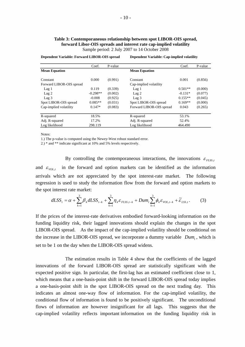
volatility for LIBOR. The market data used for the analysis are the forward-starting OIS rates for the tenors: 1m2m, 2m3m, 3m6m, 6m9m and 9m12m; the FRA rates for the tenors: 1m2m, 2m3m, 3m6m, 6m9m and 9m12m; the prices of six-month interest rate cap (i.e. composed of a 3m6m caplet) and one-year interest rate cap (i.e. composed of the 3m6m, 6m9m and 9m12m caplets). The data period is from 2 July 2007 to 14 October 2008. The principal components of the LIBOR-OIS spreads and cap-implied volatilities of the different tenors are used for the estimations in Eqs.(1) and (2).13 As shown in Table 3, the changes in the forward LIBOR-OIS spread and the cap-implied volatility are found to be positively related to the spot LIBOR-OIS spread, reflecting the inter-dependency of the information sets in the spot and derivative markets due to the common market factors.
12 Acharya and Johnson (2007) empirically investigate whether the credit default swap market acquires
information prior to the stock market. By controlling the contemporaneous interactions between the two markets, they extract the market-specified innovations and study the structure of information flow between the two markets. These innovations can then be interpreted as the market-specified information arrival to the particular markets.
13 The principal components effectively extract the “parallel shift” in the term structures.
- 10 -
Table 3: Contemporaneous relationship between spot LIBOR-OIS spread,
forward Libor-OIS spreads and interest rate cap-implied volatility Sample period: 2 July 2007 to 14 October 2008
Coef. P-value Coef. P-valueMean Equation Mean Equation
Constant 0.000 (0.991) Constant 0.001 (0.856)Forward LIBOR-OIS spread Cap-implied volatility
Lag 1 0.119 (0.339) Lag 1 0.501** (0.000)Lag 2 -0.298** (0.002) Lag 2 -0.131* (0.077)Lag 3 -0.008 (0.925) Lag 3 0.155** (0.045)
Spot LIBOR-OIS spread 0.085** (0.031) Spot LIBOR-OIS spread 0.169** (0.000)Cap-implied volatility 0.147* (0.083) Forward LIBOR-OIS spread 0.043 (0.265)
R-squared 18.5% R-squared 53.1%Adj. R-squared 17.2% Adj. R-squared 52.4%Log likelihood 298.119 Log likelihood 464.490
Notes:1.) The p-value is computed using the Newey-West robust standard error.2.) * and ** indicate significant at 10% and 5% levels respectively.
Dependent Variable: Forward LIBOR-OIS spread Dependent Variable: Cap-implied volatility
By controlling the contemporaneous interactions, the innovations tFLSS ,ε
and tVOL,ε in the forward and option markets can be identified as the information
arrivals which are not appreciated by the spot interest-rate market. The following regression is used to study the information flow from the forward and option markets to the spot interest rate market:
tLSSk
ktVOLktktFLSSk
kktk
kt DumdLSSdLSS ,
3
1,,
3
1
3
1
~εεφεηβα ++++= ∑∑∑=
−−=
−=
. (3)
If the prices of the interest-rate derivatives embodied forward-looking information on the funding liquidity risk, their lagged innovations should explain the changes in the spot LIBOR-OIS spread. As the impact of the cap-implied volatility should be conditional on the increase in the LIBOR-OIS spread, we incorporate a dummy variable tDum , which is
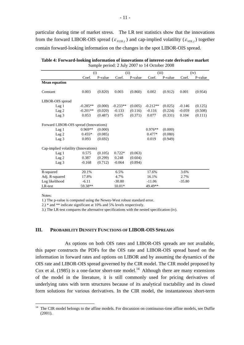
set to be 1 on the day when the LIBOR-OIS spread widens. The estimation results in Table 4 show that the coefficients of the lagged
innovations of the forward LIBOR-OIS spread are statistically significant with the expected positive sign. In particular, the first-lag has an estimated coefficient close to 1, which means that a one-basis-point shift in the forward LIBOR-OIS spread today implies a one-basis-point shift in the spot LIBOR-OIS spread on the next trading day. This indicates an almost one-way flow of information. For the cap-implied volatility, the conditional flow of information is found to be positively significant. The unconditional flows of information are however insignificant for all lags. This suggests that the cap-implied volatility reflects important information on the funding liquidity risk in
- 11 -
particular during time of market stress. The LR test statistics show that the innovations from the forward LIBOR-OIS spread ( tFLSS ,ε ) and cap-implied volatility ( tVOL,ε ) together
contain forward-looking information on the changes in the spot LIBOR-OIS spread.
Table 4: Forward-looking information of innovations of interest-rate derivative market Sample period: 2 July 2007 to 14 October 2008
Coef. P-value Coef. P-value Coef. P-value Coef. P-valueMean equation
Constant 0.003 (0.820) 0.003 (0.860) 0.002 (0.912) 0.001 (0.954)
LIBOR-OIS spreadLag 1 -0.285** (0.000) -0.233** (0.005) -0.212** (0.025) -0.146 (0.125)Lag 2 -0.201** (0.020) -0.133 (0.116) -0.116 (0.224) -0.059 (0.508)Lag 3 0.053 (0.487) 0.075 (0.371) 0.077 (0.331) 0.104 (0.111)
Forward LIBOR-OIS spread (Innovations)Lag 1 0.969** (0.000) 0.976** (0.000)Lag 2 0.455* (0.085) 0.477* (0.080)Lag 3 0.093 (0.692) 0.019 (0.949)
Cap-implied volatility (Innovations)Lag 1 0.575 (0.105) 0.722* (0.063)Lag 2 0.387 (0.299) 0.248 (0.604)Lag 3 -0.168 (0.712) -0.064 (0.894)
R-squared 20.1% 6.5% 17.6% 3.6%Adj. R-squared 17.8% 4.7% 16.1% 2.7%Log likelihood -6.11 -30.80 -11.06 -35.80LR-test 59.38** 10.01* 49.49**
Notes:1.) The p-value is computed using the Newey-West robust standard error.2.) * and ** indicate significant at 10% and 5% levels respectively.3.) The LR-test compares the alternative specifications with the nested specification (iv).
(i) (ii) (iii) (iv)
III. PROBABILITY DENSITY FUNCTIONS OF LIBOR-OIS SPREADS
As options on both OIS rates and LIBOR-OIS spreads are not available, this paper constructs the PDFs for the OIS rate and LIBOR-OIS spread based on the information in forward rates and options on LIBOR and by assuming the dynamics of the OIS rate and LIBOR-OIS spread governed by the CIR model. The CIR model proposed by Cox et al. (1985) is a one-factor short-rate model.14 Although there are many extensions of the model in the literature, it is still commonly used for pricing derivatives of underlying rates with term structures because of its analytical tractability and its closed form solutions for various derivatives. In the CIR model, the instantaneous short-term
14 The CIR model belongs to the affine models. For discussion on continuous-time affine models, see Duffie
(2001).
- 12 -
interest rates are always non-negative and their dynamics have a standard deviation proportional to square root of the level of the rates.
The dynamics of the LIBOR-OIS spread are estimated using a term-
structure model in Duffie and Singleton (1997) and Longstaff et al. (2005) which estimate the dynamics of risk premiums in interest-rate swap yields and corporate bond yields respectively. Under the CIR specification and assuming the LIBOR-OIS short-term spread independent of the level of the OIS rate, the risk-neutral dynamics of the OIS rate ( r ) and the LIBOR-OIS short-term spread ( s ) follow two uncorrelated square-root processes:
( )( ) 2222
1111
dZsdtsds
dZrdtrdr
σθκ
σθκ
+−=
+−=, (4)
where iZ are two uncorrelated standard Brownian motion (i.e. 021 =dZdZ ), iθ are the
mean-reversion levels, iκ are the speeds of mean-reversion and iσ are the volatilities,
for 2,1=i . The specification assumes both mean-reversion and conditional heteroskedasticity in the OIS rate and LIBOR-OIS spread, while keeping both quantities to be non-negative. This is consistent with the economic intuition that interest rates and the LIBOR-OIS spread are non-negative and mean-reverting.15
By aggregating the OIS rate and LIBOR-OIS spread, the LIBOR short rate
( L ) is formulated as:
srL += . (5)
This specification is commonly known as the two-factor CIR model. As overnight interest rates generally bear very low credit and liquidity risks, the credit and liquidity risk premiums contained in the OIS rate r should be very small. The OIS rate could be the best estimates of the mean expectation for a central bank’s risk-free policy rate. The LIBOR short rate L could thus be interpreted as the risk-adjusted discount rate, in which the stochastic variable s captures the liquidity and credit premiums over r . In tranquil times, given the low default risk of the banks in the LIBOR panel, the quantity s approaches zero such that the LIBOR rate is very close to the OIS rate (see the rates before the crisis emerged in August 2007 in Figure 1).
The model parameters in Eq.(4) are estimated by using the method in
Longstaff et al. (2005) which calibrates the two-factor short-rate model jointly with the risk-free interest rate curves, credit default swap (CDS) spreads and corporate bond yields, such that the credit and liquidity premiums embedded in the bond yields are separated
15 For modelling purposes, the mean-reverting component is necessary to keep the interest rate and spread to
be non-negative and non-explosive.

- 13 -
explicitly.16 The empirical results in Section II suggest that the price information embedded in the derivatives including forward OIS rates, FRAs and interest-rate caps on LIBOR can be used to perform joint-calibration of the model in Eq.(4). Because of the analytical tractability of the model, the pricing formulae (i.e. the model-implied values) of these derivatives are readily expressed in closed-form (see Appendix A). Given the model-implied values and market prices of the interest-rate derivatives, we estimate the model parameters by minimising the sum-of-square pricing errors of the prices for each trading day as:
( ) ⎪⎭
⎪⎬⎫
⎪⎩
⎪⎨⎧
⎟⎟⎠
⎞⎜⎜⎝
⎛ −+⎟⎟
⎠
⎞⎜⎜⎝
⎛ −+⎟⎟
⎠
⎞⎜⎜⎝
⎛ − ∑∑∑=Θ
n
i i
iim
i i
iim
i i
ii
CCC
SSS
LLL
222
,,,,, ˆˆ
ˆˆ
ˆˆ
min222111 σθκσθκ
, (6)
where iL is the discrete market forward LIBOR rate, iS is the discrete market
forward-starting OIS rate, iC is the market interest-rate cap, while iL , iS and iC
denote the values of the corresponding derivative instruments priced from the CIR model. The detailed pricing models of the FRA on LIBOR ( iL ), forward-starting OIS rate ( iS )
and the interest-rate cap ( iC ) on LIBOR are in Appendix A. The forward OIS and
LIBOR rates, which reflect the term structures of the interest rates, are used to gauge information on the first moment of the dynamics in the CIR model. Volatility information (i.e. the second moment) of underlying interest-rate dynamics is gauged from the interest-rate caps. The set of model parameters ( )222111 ,,;,, σθκσθκ=Θ in Eq.(4) can
then be estimated according to the pricing of iL , iS and iC , and the minimisation of
the model-pricing errors as described in Eq.(6). Using the parameters of ( )222111 ,,;,, σθκσθκ=Θ and the non-central
chi-square distributions in Cox et al. (1985) for the CIR model, the entire risk-neutral PDF ( )11 ;, ΘTrf and ( )22 ;, ΘTsf of the OIS rate and LIBOR-OIS spread are given as:
( )( ) ( )( ),2,22;22
2,,;,
2
2
2,1
μων
μνμνσθκ
χ
ω
ω
νμ
+=
⎟⎟⎠
⎞⎜⎜⎝
⎛==Θ −−
=
cp
IceTxfi (7)
where
( )( )( ) 12,,,
12
202 −===−
= −−−− σ
κθωνμσ
κ κκ cxecx
ec tT
tT , (8)
16 Another approach is the transformed maximum likelihood method in Duffie and Singleton (1997) which
segregates the model-based default risk premiums embedded in the yields of interest-rate swaps (see also Jagannathan et al. (2003)).
- 14 -
( )•ωI is the modified Bessel function of order ω , 0x denotes the current short rate at
time t and ( )μωνχ
2,22;22 +p is the PDF of the non-central chi-square distribution.17
The PDF of the LIBOR rate ( srL += ) is given by the following
convolution integral:
( ) ( ) ( ) ( )( )
( ) ( )
( ) ( )∫
∫
∫∫
Θ−Θ=
ΘΘ−=
+−ΘΘ=ΘΘ∞∞
L
L
TrLfTrdrf
TsfTsLdsf
srLTsfTrdsfdrTLg
02211
02211
02211
021
;,;,
;,;,
;,;,,;, δ
(9)
where ( )xδ is the Dirac-delta function.
To construct the term structures of the interest rates, the market data specified in Section II are used. In total, there are 12 pieces of price information for each trading day and six parameters, namely ( )1111 ,, σθκ=Θ and ( )2222 ,, σθκ=Θ to be estimated. For each trading day, the current short-term rates for the LIBOR and OIS rates are proxied by the one-month spot LIBOR and OIS rates.18
Figure 3 shows the standard deviations of the PDFs of the short-term OIS
rate and LIBOR-OIS spread in a three-month time horizon. The aggregate standard deviations of the two PDFs under the CIR model cannot be directly compared with the standard deviations of the probability implied from the market interest-rate cap prices based on Black’s (1976) model in which the interest rate follows the lognormal process, because the stochastic terms have a standard derivation proportional to r in the CIR model but to r in the Black model. However, the comparison shown in Figure 3 indicates that the calibrations of the dynamics of the short-term OIS rate and LIBOR-OIS spread are consistent with the market-implied standard derivations of the LIBOR rate.
17 According to Feller’s classification of boundary (see Karlin and Taylor (1981)), it is not difficult to show
that the boundary 0=x is a natural boundary for 0>ω such that the boundary is inaccessible and ( ) 0,0 =Θ=xf . For 01 <<− ω , 0=x becomes a regular boundary such that ( ) ∞→Θ,xf
as 0→x , with a point-mass probability accumulation around 0=x . For 1−<ω , 0=x is an exit boundary with probability outflows. For modelling purposes, 1−>ω is set , i.e. 22 σκθ > , such that the underlying variables are non-negative.
18 In other words, we assume that the term structure is flat for the tenors shorter than one month. The choice of the 1-month tenor as the proxy of the short-term rate is consistent with the empirical studies of the term-structure models in Longstaff and Schwartz (1992), Chan et. al (1992) and Bali and Wu (2006).

- 15 -
Figure 3: Standard deviations of probability density functions of OIS rate and LIBOR-OIS spread in a three-month horizon
Sample period: from 2 July 2007 to 30 June 2009
0.0
0.5
1.0
1.5
2.0
2.5
Jul-07 Oct-07 Jan-08 Apr-08 Jul-08 Oct-08 Jan-09 Apr-09
%
Implied standard deviation ofLIBOR-OIS spread
Implied standard deviation ofOIS rate
Implied standard deviation ofLIBOR under Black's model
Note: The implied standard deviations are computed using the five-day moving average
of the estimated model parameters of the dynamics of the OIS rate and LIBOR-OIS spread in Eq.(4). The results in Figure 3 reflect that the uncertainty of the LIBOR rate was
more or less identical to the uncertainty of the OIS rate before the sub-prime problem emerged in August 2007. When the crisis began to spillover to the interbank market, the attribution of the LIBOR-OIS spread to the uncertainty in the LIBOR rate increased, in particular after the Bear Stearns failure in the spring of 2008. Following the Lehman failure in mid-September 2008 that triggered the funding liquidity shock, uncertainty in the LIBOR-OIS spread became the dominant part of the LIBOR dynamics as the uncertainty in the OIS rate was almost removed when the Federal Reserve lowered the policy rate to the zero bound and expected to keep the rate at the level for a while.
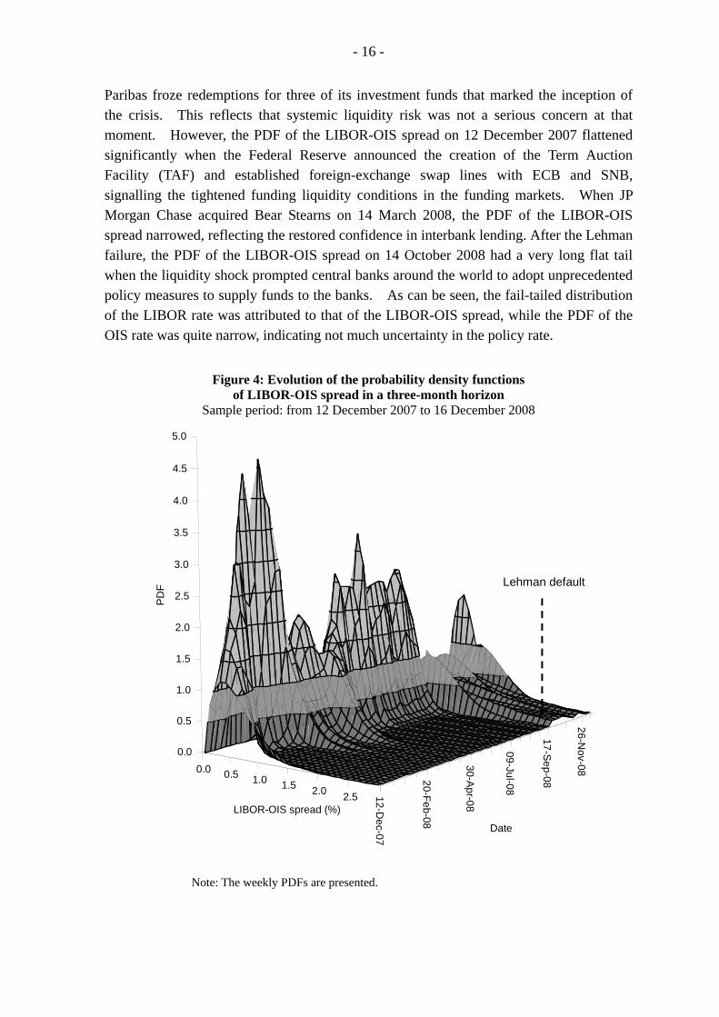
The evolution of the PDFs of the LIBOR-OIS spread illustrated in Figure 4
show that the fat-tailed distributions appeared during the crisis and the tails further extended after the Lehman failure in mid-September 2008 reflecting deepened uncertainty about the LIBOR-OIS spread (i.e. funding liquidity risk) anticipated by the market. To look at the changes in the shape of the PDFs closely, Figure 5 plots the PDFs of the LIBOR-OIS spreads, OIS and LIBOR rates on selected dates during the crisis. The PDFs of the OIS and LIBOR rates were quite similar to each other on 9 August 2007 when BNP
- 16 -
Paribas froze redemptions for three of its investment funds that marked the inception of the crisis. This reflects that systemic liquidity risk was not a serious concern at that moment. However, the PDF of the LIBOR-OIS spread on 12 December 2007 flattened significantly when the Federal Reserve announced the creation of the Term Auction Facility (TAF) and established foreign-exchange swap lines with ECB and SNB, signalling the tightened funding liquidity conditions in the funding markets. When JP Morgan Chase acquired Bear Stearns on 14 March 2008, the PDF of the LIBOR-OIS spread narrowed, reflecting the restored confidence in interbank lending. After the Lehman failure, the PDF of the LIBOR-OIS spread on 14 October 2008 had a very long flat tail when the liquidity shock prompted central banks around the world to adopt unprecedented policy measures to supply funds to the banks. As can be seen, the fail-tailed distribution of the LIBOR rate was attributed to that of the LIBOR-OIS spread, while the PDF of the OIS rate was quite narrow, indicating not much uncertainty in the policy rate.
Figure 4: Evolution of the probability density functions of LIBOR-OIS spread in a three-month horizon
Sample period: from 12 December 2007 to 16 December 2008
0.0 0.5 1.0 1.5 2.0 2.5 12-Dec-07
20-Feb-08
30-Apr-08
09-Jul-08
17-Sep-08
26-Nov-08
0.0
0.5
1.0
1.5
2.0
2.5
3.0
3.5
4.0
4.5
5.0
PD
F
LIBOR-OIS spread (%)
Date
Lehman default
Note: The weekly PDFs are presented.

- 17 -
Figure 5: Probability density functions of LIBOR-OIS spread, OIS and LIBOR rates in a three-month horizon on selected dates
9 August 2007 12 December 2007
0.0
0.2
0.4
0.6
0.8
1.0
0 1 2 3 4 5 6 7
Rate (%)
LIBOR rate
OIS rate
LIBOR-OIS spread
0.0
0.5
1.0
1.5
0 1 2 3 4 5 6 7
Rate (%)
LIBOR rate
OIS rateLIBOR-OIS spread
14 March 2008 14 October 2008
0.0
0.5
1.0
1.5
2.0
0 1 2 3 4Rate (%)
LIBOR rate
OIS rate
LIBOR-OIS spread
0.0
0.5
1.0
1.5
2.0
0 1 2 3 4 5 6Rate (%)
LIBOR rate
OIS rate
LIBOR-OIS spread
OIS rate LIBOR-OIS spread LIBOR rate
Notes: - BNP Paribas froze redemptions for three of its investment funds on 9 August 2007 - The Federal Reserve announced the creation of the Term Auction Facility (TAF) and
established foreign-exchange swap lines with ECB and SNB on 12 December 2007 - JP Morgan Chase acquired Bear Stearns on 14 March 2008. - The Federal Reserve established unlimited US-dollar swap lines with foreign central banks
on 13 October 2008. The US Treasury announced the Troubled Asset Relief Program (TARP) and FDIC announced the Temporary Liquidity Guarantee Program on 14 October 2008.
IV. ESTIMATIONS OF PROBABILITIES OF SYSTEMIC FUNDING LIQUIDITY SHOCKS
When the systemic funding liquidity problem occurred in the crisis of 2008,
the LIBOR-OIS spread surged to some unprecedented levels (over 200 basis points on 26 September 2008) after the Lehman failure over the weekend of 13 September 2008. Such level can therefore be considered as a system liquidity shock triggering boundary. When the LIBOR-OIS spread breaches the boundary, a system liquidity shock occurs and the interbank market is paralysed. Based upon the FPT approach and using the dynamics and term structure of the LIBOR-OIS spread estimated in the previous Section, the probability of the LIBOR-OIS spread passing through a pre-specified boundary in a
- 18 -
given time horizon can be estimated as a measure of the probability of a systemic funding liquidity shock.
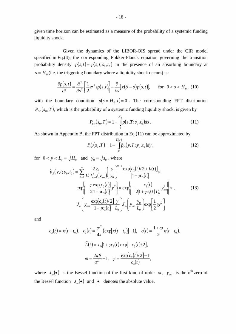
Given the dynamics of the LIBOR-OIS spread under the CIR model
specified in Eq.(4), the corresponding Fokker-Planck equation governing the transition probability density ( ) ( )00 ,;,, tstsptsp = in the presence of an absorbing boundary at
0Hs = (i.e. the triggering boundary where a liquidity shock occurs) is:
( ) ( ) ( ) ( )[ ],,,21, 2
2
2
tspss
tsspst
tsp−
∂∂
−⎥⎦⎤
⎢⎣⎡
∂∂
=∂
∂ θκσ for 00 Hs << , (10)
with the boundary condition ( ) 0,0 == tHsp . The corresponding FPT distribution
( )TsPFP ,0 , which is the probability of a systemic funding liquidity shock, is given by
( ) ( )∫−=0
0000 ,;,1,
H
FP dstsTspTsP . (11)
As shown in Appendix B, the FPT distribution in Eq.(11) can be approximated by
( ) ( )( )
∫−=TL
AA
FP dytyTypTsP~
0000 ,;,~1, , (12)
for 000 HLy =<< and 00 sy = , where
( ) ( )( )[ ]
( )( )[ ]( )
( )( )
( )[ ]( ) ⎥⎦
⎤⎢⎣⎡
⎟⎟⎠
⎞⎜⎜⎝
⎛⎟⎟⎠
⎞⎜⎜⎝
⎛
+
×⎪⎭
⎪⎬⎫
⎪⎩
⎪⎨⎧
+−×
⎪⎭
⎪⎬⎫
⎪⎩
⎪⎨⎧
+−
×+
+⎟⎟⎠
⎞⎜⎜⎝
⎛=
+∞
= +∑
2
0
0
03
2
2203
32
3
2
3
2
1
012
120
000
21exp
12/exp
12exp
12expexp
1)(2/exp2,;,~
yLyyJ
Ly
tctcyJ
yLtc
tcytctc
tctbtc
yy
yJLytytyp
nn
n
n nA
γγ
γγγ
γ
ωωωω
ω
ω
ωω
, (13)
and
( ) ( ) ( ) ( )[ ]( ) ( ) ( ),2
1,1exp4
, 00
2
302 tttbtttctttc −+
=−−=−= κωκκ
σκ
( ) ( ) ( )[ ]2/exp1~230 tctcLtL −+= γ ,
( )[ ]( ) ,12/exp,12
3
22 tc
tc −=−= γ
σκθω
where ( )•ωJ is the Bessel function of the first kind of order ω , nyω is the nth zero of
the Bessel function ( )•ωJ and • denotes the absolute value.
- 19 -
The model parameters used to estimate liquidity shock probabilities from the FPT distribution are those used to construct the PDFs of the LIBOR-OIS spread in the previous Section covering the period from 2 July 2007 to 26 September 2008 (Friday). On 29 September (Monday) the LIBOR-OIS spread breached 200 basis points after a period of turbulence in the US-dollar interbank market triggered by the Lehman failure. The interbank market malfunctioned due to the systemic liquidity shock. On the same day, the Federal Reserve authorised a US$330 billion expansion of swap lines with the Bank of Canada, BoE, Bank of Japan, Danmarks Nationalbank, ECB, Norges Bank, Reserve Bank of Australia, Sveriges Riksbank and SNB. Swap lines outstanding totalled US$620 billion. The Federal Reserve Board also expanded the Term Auction Facility (TAF), announcing an increase in the size of the 84-day maturity auction to US$75 billion and two forward TAF auctions totalling US$150 billion to provide short-term (one- to two-week) TAF credit over year-end. These unprecedented policy measures aimed to supply short-term US-dollar funds to the banks which faced liquidity shortage.
The liquidity shock probabilities using the one-month LIBOR-OIS spread
in a three-month horizon with the liquidity shock triggering boundary 0H at 200 basis
points are shown in Figure 6. The spread of 200 basis points which is observed on 26 September 2008 can also be interpreted as the credit quality of the interbank market as a whole falling into the speculative grade, reflecting that the interbank market is paralysed due to extremely high counterparty default risk.19 Figure 6(a) shows that the probabilities estimated by Eq.(12) were almost zero in most of the time before mid-September 2008. This indicates that even though uncertainty about losses incurred in banks due to the sub-prime problem increased their liquidity needs, the market considered that individual banks’ problems would not trigger a systemic liquidity shock, i.e. the US-dollar funding market was still functioning with higher risk premiums in LIBOR as indicated in the PDFs of the LIBOR-OIS spread in Figure 4.
19 The one-year implied default probability (π) given the recovery rate (ω) can be roughly estimated using
the relationship: ( ) ( ) ( )( )ωπ −−×++=+ 1111 srr ,
where r is the annualised risk-free interest rate and s is the annualised interest-rate spread. Assuming the recovery rate of 50%, a spread of 200 basis points implies a one-year default probability of about 3.88% (with r = 1%) that is close to the speculative grade’s one-year average default rate of 4.06% (see Standard & Poor’s (2009)).

- 20 -
Figure 6: First-passage-time probability of LIBOR-OIS spread in three-month horizon a.) Sample period: from 2 July 2007 to 14 October 2008
0
50
100
150
200
250
300
350
400
Jul-07 Oct-07 Jan-08 Apr-08 Jul-08 Oct-080.0
0.1
0.2
0.3
0.4
0.5
0.6
0.7
0.8
0.9
1.0
FPT probability at200 bps (RHS)
1-month spot LIBOR-OIS spread (LHS)
LIBOR-OIS spread (bps) FPT probability
FPT probability at150 bps (RHS)
b.) Sample period: from 15 August 2008 to 14 October 2008
0
100
200
300
400
500
600
700
800
15-Aug 25-Aug 04-Sep 14-Sep 24-Sep 04-Oct 14-Oct0.0
0.1
0.2
0.3
0.4
Lehman BrothersCDS spread (LHS)
FPT probability at200 bps (RHS)
1-month LIBOR-OISspread (LHS)
12 SepFPT probability
LIBOR-OIS andCDS spreads (bps)
200 bps

- 21 -
The liquidity shock probabilities then rose sharply in the second half of September. As shown in Figure 6(b), when the CDS spread of Lehman Brothers surged from the level of 300 basis points on 9 September to 642 basis points on 12 September before the firm filed for Chapter 11 bankruptcy protection on 15 September, the LIBOR-OIS spread remained steady at the level of about 50 basis points, suggesting that the market did not anticipate any systemic liquidity shock during the early stage of the event. On 18 September the liquidity shock probability became material at 0.12, when the LIBOR-OIS spread increased to 134 basis points. Given that a systemic liquidity shock is a rare event and its chance of occurrence should not be higher than a sovereign default in general, the probability of 0.12 over three months implied a substantial chance of failure of the funding markets and gave a clear warning signal of a systemic liquidity shock as compared with the almost zero probability before. Comparing with the timing of the occurrence of the liquidity shock when the LIBOR-OIS spread reached 200 basis points and the funding markets malfunctioned on 29 September, the warning signal was seven trading days in advance. The liquidity shock probability then kept on rising to almost 1 on 26 September, reflecting that the systemic liquidity problem was identified quickly after the first signal appeared.
V. CONCLUSION
This paper uses LIBOR-OIS spread as a measure of funding liquidity risk and shows that the market prices of the forward-rate contracts of OIS and LIBOR and interest-rate caps contain forward-looking information on the changes in the spot LIBOR-OIS spread. The dynamics of the LIBOR-OIS spread, which are assumed to be governed by the CIR model, are separated explicitly from the dynamics of LIBOR based on the market price information. The PDFs of the LIBOR-OIS spread constructed from its dynamics were fat-tailed distributions during the crisis in 2008 and the tails further extended after the Lehman failure reflecting deepened uncertainty about the funding liquidity risk.
Using the dynamics and term structure of the LIBOR-OIS spread, the
probability of a systemic funding liquidity shock is estimated during the crisis period. The probability deviated from zero on 18 September 2008 to 0.12, which provided an early warning signal of the systemic liquidity shock on 29 September 2008 when the interbank market was paralysed. The information content about funding liquidity risk in prices of interest-rate derivative instruments could thus improve the measurement of system-wide liquidity risk and help the financial system to be more prepared for liquidity shocks. Central banks could interpret implied probabilities of funding liquidity shocks based on the proposed approach as an indicator to serve as a basis for the development of a set of potential early warning indicators
- 22 -
Appendix A: Pricing the financial instruments A1. Pricing zero-coupon bonds and interest rate forwards
The forward rate is the interest rate paid for a loan in a future period from
time 1T to 2T . At current time t , the forward interest rate can be formulated as:
( ) ( )( ) ⎥
⎦
⎤⎢⎣
⎡−
−= 1
,,1,;
2
1
1221 TtP
TtPTT
TTtF , for 21 TTt ≤≤ (A1)
where ( )1,TtP and ( )2,TtP are the present value of $1 to be received at time 1T and 2T respectively.
Regarding an interest rate which bear credit and liquidity premiums, the quantity ( )TtP , can be interpreted as the price of a zero-coupon bond matures at time T discounted by the risk-adjusted interest rate. To derive the model-implied forward rates for the OIS and LIBOR rates, we can make use of the model prices of zero-coupon bonds discounted by the OIS and LIBOR rates. The value of a T-maturity zero-coupon bond
( )TtPOIS , discounted by the OIS rate is given by:
( ) ( )⎥⎥⎦
⎤
⎢⎢⎣
⎡⎟⎟⎠
⎞⎜⎜⎝
⎛−=Θ≡ ∫ ττ drETtPTtP
T
t
QOISOIS exp;,, 1 , for Tt ≤≤ τ (A2)
where ( )1111 ,, σθκ≡Θ denotes the model parameters for r . Here Q denotes the risk-neutral probability measure under the no-arbitrage environment. Similarly, the value of a T-maturity zero-coupon bond ( )TtPLIBOR , discounted by the LIBOR rate is given by:
( ) ( )
⎥⎥⎦
⎤
⎢⎢⎣
⎡⎟⎟⎠
⎞⎜⎜⎝
⎛−
⎥⎥⎦
⎤
⎢⎢⎣
⎡⎟⎟⎠
⎞⎜⎜⎝
⎛−=
⎥⎥⎦
⎤
⎢⎢⎣
⎡⎟⎟⎠
⎞⎜⎜⎝
⎛−=
ΘΘ≡
∫∫
∫
ττ
τ
ττ
τ
dsEdrE
dLE
TtPTtP
T
t
QT
t
Q
T
t
Q
LIBORLIBOR
expexp
exp
,;,, 21
, for Tt ≤≤ τ (A3)
where ( )1111 ,, σθκ≡Θ and ( )2222 ,, σθκ≡Θ are the model parameters for r and s . The last equality in Eq.(A3) follows the assumption of the two stochastic variables r and s being independent. The model-implied value of the zero-coupon bond discounted by the OIS rate depends solely on the dynamics ( ){ }1111 ,,; σθκ≡Θr , while that of the zero-coupon bond discounted by the LIBOR rate depends on the aggregate dynamics of
( ){ }1111 ,,; σθκ≡Θr and ( ){ }2222 ,,; σθκ≡Θs . Given the prices of the zero-coupon bonds, the forward rates of OIS and
LIBOR for the period 1T to 2T can be readily expressed respectively using Eq.(A1) as:
- 23 -
( ) ( )( ) ⎥
⎦
⎤⎢⎣
⎡−
−= 1
,,1,;
2
1
1221 TtP
TtPTT
TTtFOIS
OISOIS , for 21 TTt ≤≤ (A4)
and
( ) ( )( ) ⎥
⎦
⎤⎢⎣
⎡−
−= 1
,,1,;
2
1
1221 TtP
TtPTT
TTtFLIBOR
LIBORLIBOR , for 21 TTt ≤≤ (A5)
where ( )TtPOIS , and ( )TtPLIBOR , denote the values of zero-coupon bonds with maturity at
time T discounted by the OIS rate and LIBOR rate respectively. It is not difficult to show that ( )TtPOIS , and ( )TtPLIBOR , can be expressed in terms of the standard pricing
formula of a zero-coupon bond (T-maturity) under the one-factor CIR model as:
( ) ( )10 ;,,, Θ= TtrPTtP CIROIS , (A6)
and ( ) ( ) ( )2010 ;,,;,,, ΘΘ= TtsPTtrPTtP CIRCIRL (A7)
respectively. Here 0r and 0s denote the current short-term rate and spread. The
zero-coupon bond under the CIR model is expressed in a closed-form solution as:
{ }( ) [ ],),(exp),(,,;,, 00 TtBxTtATtxPCIR −==Θ σκθ (A8)
with
( )( )[ ]( ) ( )[ ]( ) ,
1exp22/exp2),(
2
2σ
κθ
γγκγγκγ
⎥⎦
⎤⎢⎣
⎡−−++
−+=
tTtTTtA (A9)
( )[ ]( )( ) ( )[ ]( ) ,
1exp21exp2),(
−−++−−
=tT
tThTtBγγκγ
γ (A10)
where 22 2σκγ += . A2. Pricing options on zero-coupon bonds
An interest-rate cap is composed of a portfolio of individual interest-rate
caplets of different maturities, in which an interest caplet is a European-style call option which pays the buyer the interest-rate difference between the actual LIBOR rate and the strike price K , multiplied by the contractual notional amount. The payment is usually paid in arrears: suppose time T is the maturity of the contract and the underlying interest rate is for a τ -period, then the payment occurs at time τ+T . At maturity, an interest-rate caplet with notional amount of $1 has the effective payoff:
( )[ ]0,max1
1,
,
ττ τ
τ
KLL
Caplet TTTT
−+
= ++
, (A11)
- 24 -
where τ+TTL , is the τ -period actual LIBOR rate at maturity. In theory, the payoff of an
interest-rate caplet can be replicated by a put option on a )( τ+T -maturity zero-coupon bond (discounted by the LIBOR rate) as:
( )[ ] ( ) ( )[ ]0,,max10,max1
1,
,
ττττ τ
τ
+−+=−+ +
+
TTPPKKLL LKTT
TT
, (A12)
where ( )τ+TTPL , is the time T value of a zero-coupon bond with maturity at τ+T ,
τKPK +
=1
1 is the strike price of the bond put option and $ ( )τK+1 is the notional
amount of the option. In other words, an interest-rate caplet linked to LIBOR is just a put option on a zero-coupon bond discounted by the LIBOR rate. Therefore, at current time t , the no-arbitrage price of an interest rate caplet is readily expressed as:
( ) ( ) ( )τττ +×+= TTtVKTtV ;,1;, putcaplet , for Tt ≤ (A13)
where
( ) ( )[ ]⎥⎦⎤
⎢⎣⎡ +−⎟
⎠⎞
⎜⎝⎛
∫−=+ 0,,maxexp;,put ττ TTPPdsLETTtV LK
T
ts
Q , (A14)
is the price of a put option on a )( τ+T -maturity zero-coupon bond and KP is the strike price of the put option.
Under the two-factor CIR model, the price of a call option on a
2T -maturity zero-coupon bond with maturity at time T is given by:
( ) ( )
( )
( ) ( ) ( ) ( )22112
2
2120callcall
;,;,,;,
)0,,max(exp
,;,;,,
ΘΘ=
⎥⎦⎤
⎢⎣⎡ −⎟
⎠⎞
⎜⎝⎛
∫−=
ΘΘ=
∫∫ TsfTrfTTLPdrdsTtP
PTTPdsLE
TTtLVTtV
LL
KL
T
ts
Q (A15)
where t is the current time, 2T is the maturity of the underlying zero-coupon bond, srL += is the LIBOR rate at option maturity T and KP is the strike price of the
option. As shown in Chen and Scott (1992), the call option price in Eq.(A15) can be expressed as:
( ) ( ) ( )
( ) ( ),~,~;,;~,~,
,;,;,,,
2121212
212121call
δδννξξχ
δδννξξχ
TTPP
TtPTtV
LK
L −= (A16)
where ( )212121 ,;,;, δδννξξχ is the bivariate chi-square distribution function
( ) ( )dzzgzG 220
112
11212121 ,;,;,;,;,
2
δνδνξξ
ξδδννξξχξ
×⎟⎟⎠
⎞⎜⎜⎝
⎛−= ∫ , (A17)

- 25 -
( )11,; δν•G is the cumulative distribution function and ( )11,; δν•g is the density function
of a non-central chi-square random variable. ( )21,TTPL can be interpreted as the price of a
forward zero-coupon bond written at the start date at 1T with maturity at 2T . The input arguments in Eq.(A16) are:
,4,~2~,2 2**
i
iiiiiiiii yy
σθκνψξψξ === (A18)
( )[ ] ( )[ ],~exp~,exp 22
i
iiiti
i
iiiti
tTytTyψ
γφδψ
γφδ −=
−= (A19)
with
( ) ,,2~,2 222 ⎟⎟⎠
⎞⎜⎜⎝
⎛+
++=⎟⎟
⎠
⎞⎜⎜⎝
⎛ ++= TTBi
i
iiii
i
iiii σ
κγφψ
σκγ
φψ (A20)
( ) ( )
( ) ( )[ ]( ) ,2,1exp
2,
,
,,ln
222
2
2221
*iii
ii
ii
i
Ki tTTTB
PTTATTA
y σκγγσ
γφ +=
−−=
⎥⎦
⎤⎢⎣
⎡
= (A21)
( ) ( )( )[ ]( ) ( )[ ]( ) ,
1exp22/exp2,
2
2
2
22
i
ii
TTTTTTA
iiii
iiii
σ
θκ
γγκγγκγ
⎥⎦
⎤⎢⎣
⎡−−++
−+= (A22)
( ) ( )[ ]( )( ) ( )[ ]( ) ,
1exp21exp2,
2
22 −−++
−−=
TTTTTTB
iiii
iii γγκγ
γγ (A23)
for i = 1,2, where 01 ry t = and 02 sy t = . The corresponding put option on the zero-coupon
bond is obtained by put-call parity as:
( ) ( ) ( ) ( )222call2put ,,,;,; TTPPTtPTTtVTTtV LKL +−= . (A24)
Then, the price of an interest rate caplet is:
( ) ( ) ( ) ( ) ( )[ ]τττττ +++−+×+= TTPPTtPTTtVKTtV LKL ,,,;1;, callcaplet . (A25)

- 26 -
Appendix B: First-passage-time probability of the LIBOR-OIS spread Assuming the short-rate dynamics of the LIBOR-OIS spread following
Eq.(4), the corresponding Fokker-Planck equation governing the transition probability density ( ) ( )00 ,;,, tstsptsp = in the presence of an absorbing boundary at 0Hs = is
given by Eq.(10). The initial and boundary conditions are specified as:
( ) ( ) ( ) ( ) 0,0,0,,, 000 ====−== tsptHspssttsp δ , (B1)
where 0t is the current time, T is the time horizon of the assessment and Ttt ≤≤0 .
The boundary 0=s is assumed to be inaccessible (by setting 022 >
σκθ ). The
corresponding FPT distribution function ( )TsPFP ,0 is given by Eq.(11).20
Taking the change of variable sy = , Eq.(10) becomes
( ) ( ) ( ) ( ),,~21,~
21,~
81,~
22
22 typ
yytyp
yy
ytyp
ttyp
⎟⎟⎠
⎞⎜⎜⎝
⎛++
∂∂
⎟⎟⎠
⎞⎜⎜⎝
⎛−+
∂∂
=∂
∂ νκνκσ (B2)
with
( ) ( ) ,41,),(
21,~ 2σκθν −== tyspy
typ (B3)
for 000 HLy =<< . Based upon the result in Lo and Hui (2006), a class of
approximate solution of ( )00 ,;,~ tytypA to Eq.(B2) subject to the absorbing boundary
condition at ( ) 0,~0 == tLyp is given by Eq.(13).21 The approximate solution ( )typA ,~
satisfies the Fokker-Planck equation and the parametric class of absorbing boundary condition of ( )( ) ,0,~~ == ttLspA for tt ≤0 (B4)
20 It is not difficult to show that the corresponding FPT density function can also be formulated as
( ) ( ) ( )0
,21,
, 2
Hs
FPFP s
tspst
tsPtsp
=∂∂
=∂
∂= σ ,
by substituting the Fokker-Planck equation into Eq.(11). 21 The roots of the Bessel function of non-integer order have to be found numerically. The behaviour of
Bessel functions and its zeros are however well documented in the literature. For example, for positive ω, the first root has the approximation:
3/73/513/13/11 043.00908.000397.003315.185575.1 ωωωωωωω +−−++= −−−y ;
for large argument, the roots are distributed approximately evenly at the interval of size π. See Abramowitz and Stegun (1970) for details.

- 27 -
with ( ) ( ) ( )[ ]2/exp1~
230 tctcLtL −+= γ . The parameter γ is a real adjustable parameter
controlling the movements of the absorbing boundary ( )tL~ . As demonstrated in Lo and Hui (2006), we can determine the upper and lower bounds for the exact FPT distribution function by choosing the parameter γ . We use the upper bound solution to obtain conservative estimates of the probabilities of funding liquidity shocks. It is not difficult to show that the upper bound of the FPT distribution is given by Eq.(12) by choosing the adjustable parameter ( )[ ]{ } ( )TcTc 32 /12/exp −=γ .

- 28 -
REFERENCES Abramowitz, M., Stegun, I. A. (1972), Handbook of Mathematical Functions with
Formulas, Graphs, and Mathematical Tables, Dover Publications, New York. Acharya, V. V., Johnson, T.C. 2007. Insider Trading in Credit Derivatives. Journal of
Financial Economics 84, 110-141. Bali, T. G., Wu, L. 2006. A Comprehensive Analysis of the Short-Term Interest-Rate
Dynamics. Journal of Banking and Finance 30, 1269-1290. Black, F., 1976. The Pricing of Commodity Contracts. Journal of Financial Economics 3,
167-179. Brockman, P., Turtle, H. J., 2003. A Barrier Option Framework for Corporate Security
Valuation. Journal of Financial Economics 67, 511-529. Campa, J. M., Chang, P. H. K., 1996. Arbitrage-Based Tests of Target-Zone Credibility:
Evidence from ERM Cross-Rate Options. American Economic Review 86, 726-740. Chan, K. C., Karolyi, G. A., Longstaff, F. A., Sanders, A. B. 1992. An Empirical
Comparison of Alternative Models of the Short-Term Interest Rate. Journal of Finance 47(3), 1209 – 1227.
Chen, R., Scott L. 1992. Pricing Interest Rate Options in a Two-Factor Cox-Ingersoll-Ross
Model of the Term Structure. Review of Financial Studies 5(4), 613-636. Cox, J. C., Ingersoll, J. E. and Ross, S. A. 1985. A Theory of the Term Structure of Interest
Rates. Econometrica 53(2), 385-408. Duffie, D. 2001. Dynamic Asset Pricing Theory (Third Edition). Princeton University
Press, Princeton, New Jersey. Duffie, D. and Singleton , K. J. 1997. An Econometric Model of the Term Structure of
Interest-Rate Swap Yields. Journal of Finance 52(4), 1287-1321. Hui, C. H. and Chung, T. K. 2009. Pricing Anomalies in interest rate markets during the
financial crisis of 2007-2009, Working Paper, Hong Kong Monetary Authority. Available at SSRN: http://ssrn.com/abstract=1492965.
Hui, C. H., Lo, C. F., 2009. A Note on Estimating Realignment Probabilities – A
First-Passage-Time Approach. Journal of International Money and Finance 28, 804-812.

- 29 -
Jagannathan, R., Kaplin, A. and Sun, S. 2003. An Evaluation of Multi-Factor CIR Models
Using LIBOR, Swap Rates and Cap and Swaption prices. Journal of Econometrics, 116, 113-146
Jarrow, R., Protter, P., 2004. Structural Versus Reduced Form Models: A New Information
Based Perspective. Journal of Investment Management 2, 1–10. Karlin, S, Taylor, H. M., 1981. A Second Course in Stochastic Processes, Academic Press,
New York. Lo, C. F., Hui, C. H., 2006. Lie-Algebraic Approach for Pricing Moving Barrier Options
with Time-Dependent Parameters. Journal of Mathematical Analysis and Application 323, 1455-1464.
Longstaff, F. A., Schwartz, E. S. 1992. Interest Rate Volatility and the Term Structure: A
Two-Factor General Equilibrium Model. Journal of Finance 47(4), 1259-1282. Longstaff, F. A., Mithal, S. and Neis, E. 2005. Corporate Yield Spreads: Default Risk or
Liquidity? New Evidence from the Credit Default Swap Market. Journal of Finance 60(5), 2213-2253.
Malz, A.M., 1996. Using Option Prices to Estimate Realignment Probabilities in the
European Monetary System: the Case of Sterling-Mark. Journal of International Money and Finance 15, 717-48.
McAndrews J., Sarkar A., Wang Z. 2008. The Effect of the Term Auction Facility on the
London Interbank Offered Rate, Federal Reserve Bank of New York Staff Report 335.
McGuire, P., von Peter, G.. 2009. The US Dollar Shortage in Global Banking. BIS
Quarterly Review (March 2009), 47-63. Merton, R. C., 1974. On the Pricing of Corporate Debt: The Risk Structure of Interest
Rates. Journal of Finance 29, 449-470. Michaud, F. M., Upper, C. 2008. What Drives Interbank Rates? Evidence from the LIBOR
Panel. BIS Quarterly Review (March 2008), 47-58. Mizrach, B., 1996. Did Option Prices Predict the ERM Crisis? Working Paper no. 96-10,
Rutgers University. Schwarz, K. 2009. Mind the Gap: Disentangling Credit and Liquidity in Risk Spreads.
Working Paper, Columbia University Graduate School of Business.

- 30 -
Söderlind, P., 2000. Market Expectations in the UK Before and After the ERM Crisis.
Economica 67, 1-18. Standard & Poor’s. 2009. Default, Transition, and Recovery: 2008 Annual Global
Corporate Default Study And Rating Transitions. Taylor, J. B., Williams, J. C., 2009. A Black Swan in the Money Market. American
Economic Journal: Macroeconomics 1(1), 58–83.