using r for hedge fund of funds risk managementfunds risk management
TRANSCRIPT

Using R for Hedge Fund of Funds Risk ManagementFunds Risk Management
R/Finance 2009: Applied Finance with RR/Finance 2009: Applied Finance with RUniversity of Illinois Chicago, April 25, 2009
Eric ZivotProfessor and Gary Waterman Distinguished Scholar,
Department of EconomicsAdjunct Professor, Departments of Finance and Statistics
University of Washington
OutlineOutline
• Hedge fund of funds environmentHedge fund of funds environment• Factor model risk measurement
i l i i i• R implementation in corporate environment• Dealing with unequal data histories• Some thoughts on S-PLUS and S+FinMetrics
vs. R in Finance
© Eric Zivot 2009

Hedge Fund of Funds Environment• HFoFs are hedge funds that invest in other hedge
funds– 20 to 30 portfolios of hedge funds– Typical portfolio size is 30 funds
• Hedge fund universe is large: 5000 live funds– Segmented into 10-15 distinct strategy types
• Hedge funds voluntarily report monthly performance to commercial databases– Altvest, CISDM, HedgeFund.net, Lipper TASS,
CS/Tremont, HFR• HFoFs often have partial position level data on
invested funds © Eric Zivot 2009
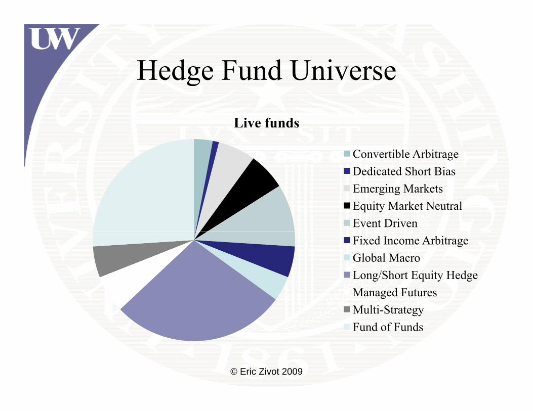
Hedge Fund UniverseHedge Fund UniverseLive funds
Convertible ArbitrageDedicated Short BiasEmerging MarketsEquity Market NeutralEvent DrivenFixed Income ArbitrageGlobal MacroLong/Short Equity HedgeManaged FuturesMulti-StrategyFund of Funds
© Eric Zivot 2009

Characteristics of Monthly ReturnsCharacteristics of Monthly Returns
• Reporting biasesReporting biases– Survivorship, backfill
N l b h i• Non-normal behavior– Asymmetry (skewness) and fat tails (excess
k t i )kurtosis)• Serial correlation
– Performance smoothing, illiquid positions• Unequal histories
© Eric Zivot 2009

Characteristics of Hedge Fund DataCharacteristics of Hedge Fund Datafund1 fund2 fund3 fund4 fund5
Observations 122.0000 107.0000 135.0000 135.0000 135.0000NAs 13.0000 28.0000 0.0000 0.0000 0.0000Minimum -0.0842 -0.3649 -0.0519 -0.1556 -0.2900Quartile 1 -0.0016 -0.0051 0.0020 -0.0017 -0.0021Median 0.0058 0.0046 0.0060 0.0073 0.0049Arithmetic Mean 0.0038 -0.0017 0.0063 0.0059 0.0021Geometric Mean 0.0037 -0.0029 0.0062 0.0055 0.0014Quartile 3 0.0158 0.0129 0.0127 0.0157 0.0127Maximum 0.0311 0.0861 0.0502 0.0762 0.0877Variance 0.0003 0.0020 0.0002 0.0008 0.0013Stdev 0.0176 0.0443 0.0152 0.0275 0.0357Skewness -1.7753 -5.6202 -0.8810 -2.4839 -4.9948Kurtosis 5.2887 40.9681 3.7960 13.8201 35.8623Rho1 0.6060 0.3820 0.3590 0.4400 0.383
Sample: January 1998 – March 2009
© Eric Zivot 2009
p y

Factor Model Risk Measurement in HFoFs Portfolio
• Quantify factor risk exposuresQuantify factor risk exposures– Equity, rates, credit, volatility, currency,
commodity etccommodity, etc.• Quantify tail risk
V R ETL– VaR, ETL• Risk budgeting
– Component, incremental, marginal• Stress testing and scenario analysis
© Eric Zivot 2009

Commercial ProductsCommercial Products
www riskdata com www finanalytica comwww.riskdata.com www.finanalytica.com
Very expensive! R is not!
© Eric Zivot 2009
Very expensive! R is not!

Factor Model: MethodologyFactor Model: Methodology1 1 , it i i t ik kt itR F Fα β β ε= + + + +
1i i it
i t t Tα ε′= + +tβ F
F
1, , ; , ,~ ( , )
i
t F
i n t t T= =
F μ Σ… …
F2,
( )
~ (0, )t F
it iεε σ
μ
cov( , ) 0 for all , and
cov( ) 0 forjt itf j i t
i j
ε
ε ε
=
= ≠© Eric Zivot 2009
cov( , ) 0 for it jt i jε ε = ≠

Practical ConsiderationsPractical Considerations
• Many potential risk factors ( > 50)Many potential risk factors ( > 50)• High collinearity among some factors
i k f di i li /• Risk factors vary across discipline/strategy• Nonlinear effects• Dynamic effects• Time varying coefficientsTime varying coefficients• Common histories for factors; unequal
histories for fund performancehistories for fund performance© Eric Zivot 2009
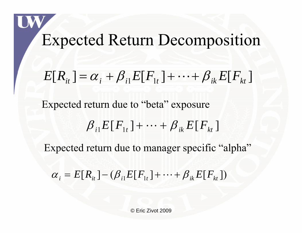
Expected Return DecompositionExpected Return Decomposition
][][][ FEFERE ββ ][][][ 11 ktiktiiit FEFERE ββα +++=
E t d t d t “b t ”
][][ 11 ktikti FEFE ββ ++
Expected return due to “beta” exposure
11 ktikti ββ
Expected return due to manager specific “alpha”
])[][(][ 11 ktiktiiti FEFERE ββα ++−=
© Eric Zivot 2009

Variance Decompositionp
2var( ) var( ) var( )R ε σ′ ′= + = +β F β β Σ β ,var( ) var( ) var( )it i t i it i i iR εε σ= + = +Fβ F β β Σ β
systematic specific
Variance contribution due to factor exposures
)var()var()var( 22
221
21 ktktt FFF βββ +++
)cov(2)cov(2 FFFF ++ ββββ
Variance contribution due to covariances between factors
© Eric Zivot 2009
),cov(2),cov(2 112121 kttkkktt FFFF −−++ ββββ
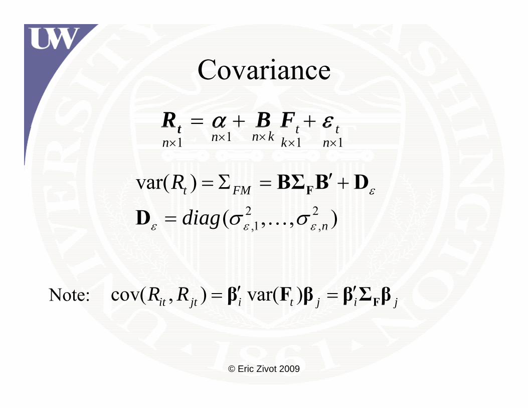
CovarianceCovariance
t t= + +tR B Fα ε
( )R ′Σ +BΣ B D
11 1 1t tn knn k n××× × ×
+ +tR B Fα ε
2 2,1 ,
var( )
( , , )t FM
n
R
diagε
ε ε εσ σ
′= Σ = +
=FBΣ B D
D …,1 ,nε ε ε
cov( , ) var( )it jt i t j i jR R ′ ′= = Fβ F β β Σ βNote:
© Eric Zivot 2009

Portfolio AnalysisPortfolio Analysis
1( , , ) portfolio weightsnw w ′= =w …
R ′+′+′=′= εwBFwαwRw
1( , , ) p gn
n
itit
n
ii
n
ii
n
iti
tttpt
wwwRw
R
εα +′+==
++==
∑∑∑∑ Fβ
εwBFwαwRw
pttpp
iitit
iii
iii
iiti wwwRw
εα
εα
+′+=
++ ∑∑∑∑====
Fβ
Fβ1111
pttpp
© Eric Zivot 2009

Portfolio Variance DecompositionPortfolio Variance Decomposition
′+′′′R2 )()( DBBΣR
′′=
′+′′=′==
Fsystematicp
Ftptp R2
,
2 )var()var(
σ
σ
wBBΣw
DwwwBBΣwwRw
∑=′=n
iiispecificp
yp
w1
2,
2,
,
εσσ Dww2
2,2 systematicp
pRσ
σ=
=i 1 pσ
2 2 2, , covariance terms
k
p systematic p F p p j jjσ β β β σ′= Σ = +∑1
2 2 2covariance terms
j
k
p systematic p j jjσ β σ
=
= −∑© Eric Zivot 2009
, ,1
p systematic p j jjjβ
=∑
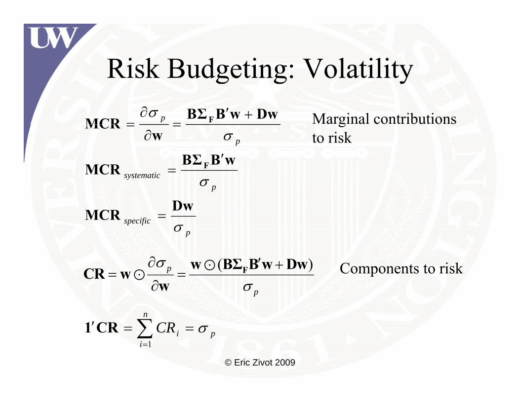
Risk Budgeting: VolatilityRisk Budgeting: Volatilitypσ DwwBBΣMCR F +′=
∂= Marginal contributions
systematic
pσ
wBBΣMCR
wMCR
F ′=
=∂
= gto risk
specific
psystematic
σ
σ
DwMCR =pσ
( )pσ∂ ′ += = Fw BΣ B w DwCR w Components to risk
pσ= =
∂CR w
w
∑ ==′n
CR σCR1
p
© Eric Zivot 2009
∑=
==i
piCR1
σCR1

Tail Risk MeasuresTail Risk MeasuresValue-at-Risk (VaR)
1( )VaR q Fα α α−= − = −
of returns F CDF R=
Expected Shortfall (ES)
[ | ]ES E R R VaR≤[ | ]ES E R R VaRα α= − ≤
© Eric Zivot 2009

Tail Risk Measures: Normal DistributionTail Risk Measures: Normal Distribution
2 2~ ( , ), p p p p FMR N w wμ σ σ ′= Σ1, ( )
1
Np pVaR z zα α αμ σ α−= − − × = Φ
1 ( )Np pES zα αμ σ φ
α= −
See functions in PerformanceAnalytics
© Eric Zivot 2009

Tail Risk Measures: Non-Normal DistributionsTail Risk Measures: Non Normal Distributions
Use Cornish-Fisher expansion to account for asymmetry p y yand fat tails
CFi iVaR zα αμ σ= − − ×
( ) ( ) ( )2 3 3 21 1 11 3 2 56 24 36
i i
i i i iz skew z z ekurt z z skew
α α
α α α α α
μ
σ ⎡ ⎤+ − − − − + −⎢ ⎥⎣ ⎦
:CFESαFormula given in Boudt, Peterson and Croux (2008) "Estimation and Decomposition of Downside Risk for Portfolios with Non-Normal Returns," Journal of Risk and implementation in PerformanceAnalytics
© Eric Zivot 2009
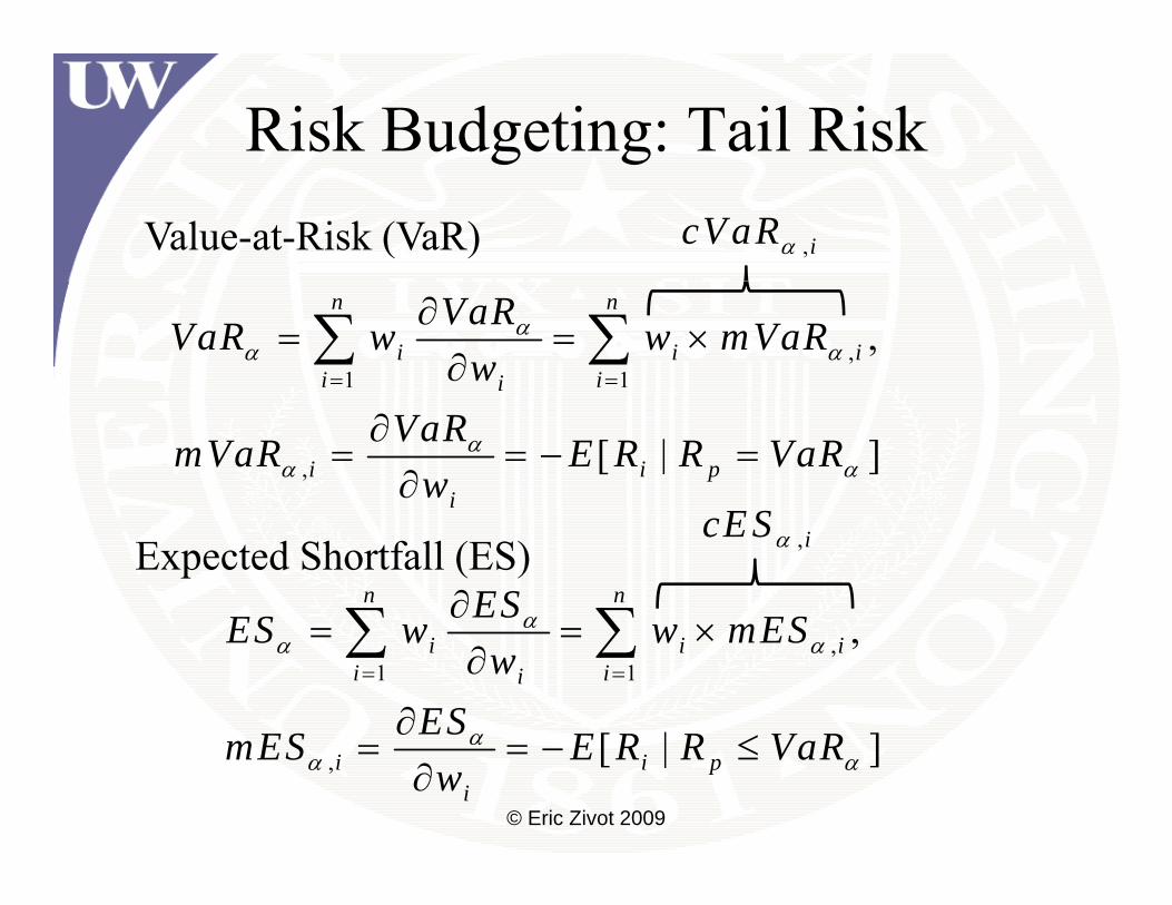
Risk Budgeting: Tail RiskValue-at-Risk (VaR) ,icV aRα
,1 1
,n n
i i ii ii
VaRVaR w w mVaRw
αα α
= =
∂= = ×
∂∑ ∑
, [ | ]i i pi
VaRmVaR E R R VaRw
αα α
∂= = − =
∂
Expected Shortfall (ES)n nESES ESα∂∑ ∑
,icE Sα
,1 1
,
[ | ]
i i ii ii
ES w w mESw
ESES E R R V R
αα α
α
= =
= = ×∂
∂≤
∑ ∑
© Eric Zivot 2009
, [ | ]i i pi
mES E R R VaRw
αα α= = − ≤
∂

Risk Budgeting: Explicit FormulasRisk Budgeting: Explicit Formulas
• Normal distributionNormal distribution– See Jorian (2007) or Dowd (2002)
N l di t ib ti i C i h Fi h• Non-normal distribution using Cornish-Fisher expansion
S B d P d C (2008) "E i i– See Boudt, Peterson and Croux (2008) "Estimation and Decomposition of Downside Risk for Portfolios with Non Normal Returns " Journal ofPortfolios with Non-Normal Returns, Journal of Risk and implementation in PerformanceAnalytics
© Eric 9ivot 2008

Risk Budgeting: SimulationRisk Budgeting: Simulation1{ } simulated returnsM
it tR M= =
Method 1: Brute Force
, , , i ii i
VaR ESmVaR mESw w
α αα α
Δ Δ≈ =
Δ Δi i
Method 2: Average Rit around values for which Rpt = VaRVaRα
, ,: :
, i it i itt R VaR t R VaR
mVaR R mES Rα αε= ± ≤
≈ − ≈ −∑ ∑
© Eric Zivot 2009
: :pt ptt R VaR t R VaRα αε= ± ≤

R Functions for Factor Model Risk Analysis
Function FunctionfactorModelCovariance normalESfactorModelRiskDecomposition normalPortfolioESnormalVaR normalMarginalESnormalVaR normalMarginalESnormalPortfolioVaR normalComponentESnormalMarginalVaR modifiedESnormalComponentVaR modifiedPortfolioESnormalVaRreport modifiedESreportmodifiedVaR simulatedMarginalVaRmodifiedPortfolioVaR simulatedComponentVaRmodifiedMarginalVaR simulatedMarginalESmodifiedComponentVaR simulatedComponentESmodifiedComponentVaR simulatedComponentES
© Eric Zivot 2009
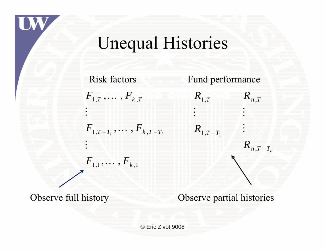
Unequal HistoriesUnequal Histories
Risk factors Fund performance
1, ,, ,T k TF F… 1,TRRisk factors Fund performance
,n TR
1, ,, ,i iT T k T TF F− −…
11,T TR −
R
1,1 ,1, , kF F…, nn T TR −
Observe full history Observe partial histories
© Eric Zivot 9008

Example Portfolio: Unequal Histories of Individual FundsX1
6593
9
0.04
0.00
X104
314
-0.0
50.
000.
05
-0.0
8-0
0.0
0.1 -0.1
5-0
.10
00
X295
54
0.3
-0.2
-0.1
0
X153
684
08-0
.04
0.00
-00
0.02
0.04
69
-0.0
0.02
45
-0.0
40.
00
X113
16
-0.0
6-0
.02
X156
14
© Eric Zivot 2009
1998 2000 2002 2004 2006 2008 1998 2000 2002 2004 2006 2008

Implication of Unequal HistoriesImplication of Unequal Histories
• Can’t fit factor models to some fundsCan t fit factor models to some funds– Need to create proxy factor model
St ti ti hi t i (t t d d t )• Statistics on common histories (truncated data) may be unreliable
• Difficult to compute non-normal tail risk measures
© Eric Zivot 2009
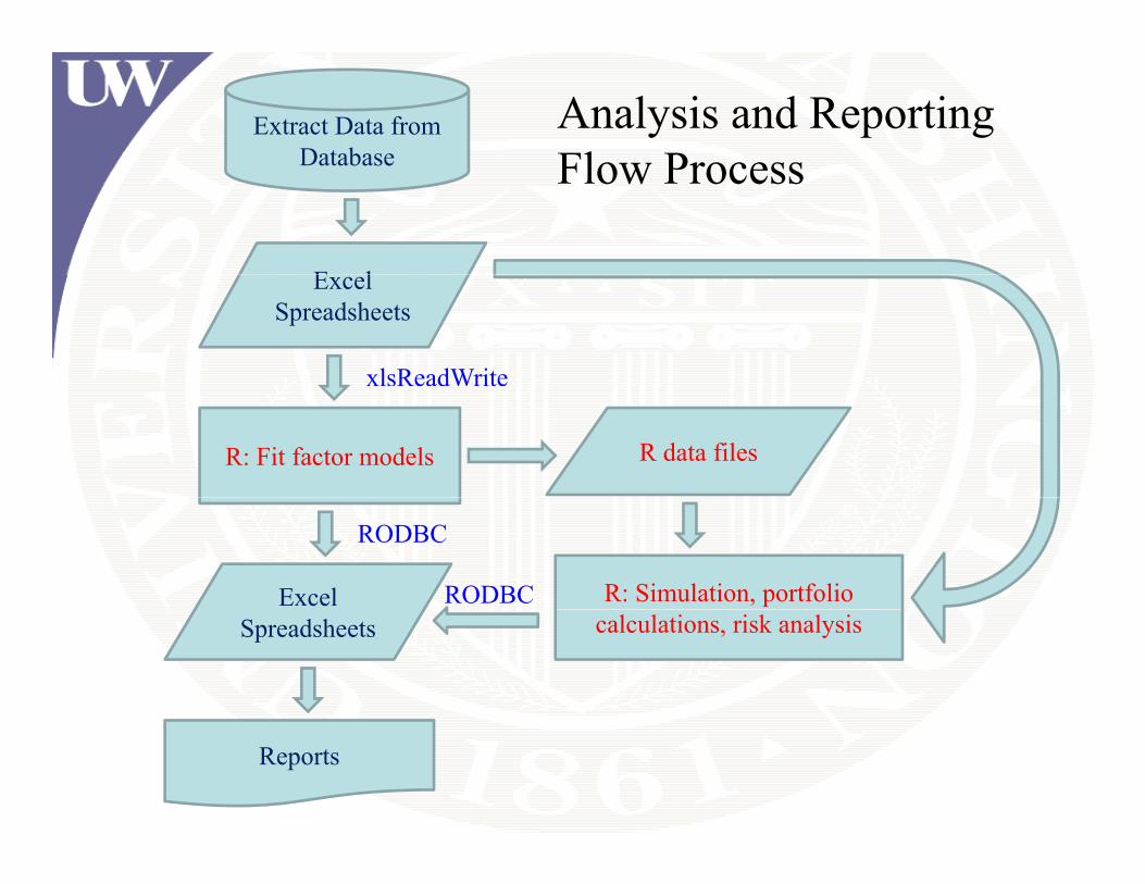
Extract Data from Database
Analysis and Reporting Flow ProcessDatabase
E l
Flow Process
Excel Spreadsheets
xlsReadWrite
R: Fit factor models R data files
Excel R: Simulation, portfolio
RODBC
RODBCSpreadsheets calculations, risk analysis
Reports

S ffi i
Factor Model ConstructionSufficient history? No
Yes
Fit factor model :Variable selection: leaps, MASSCollinearity diagnostics: card i i d l
Create proxy factor model from models with sufficient history
dynamic regression: dynlm
R data file
© Eric Zivot 2009

Evaluation of Fitted Factor ModelsEvaluation of Fitted Factor Models
• Graphical diagnosticsGraphical diagnostics– Created plot method appropriate for time series
regressionregression. • Stability analysis
CUSUM t t h– CUSUM etc: strucchange– Rolling analysis: rollapply (zoo)
Ti i dl– Time varying parameters: dlm• Dynamic effects
– dynlm, lmtest© Eric Zivot 2009

Diagnostic Plots: Example Fund0.
02p ,
0.00
ce
4-0
.02
nthl
y pe
rform
anc
-0.0
6-0
.04
Mon
-0.0
8-
2005 2006 2007 2008 2009
ActualFitted
© Eric Zivot 2008
Index
2005 2006 2007 2008 2009

0.6
0.8
1.0
60
Time Series Regression Residual diagnosticsAC
F
-0.2
0.0
0.2
0.4
01.
0 Den
sity
3040
50
PAC
F
-0.2
0.0
0.2
0.4
0.6
0.8
010
20
Lag
5 10 15
Returns
-0.04 -0.02 0.00 0.02
OLS-based CUSUM test
1.5
.02
uatio
n pr
oces
s
00.
51.
0
al Q
uant
iles 0.
000.
Em
piric
al fl
uctu
-1.0
-0.5
0.0
Em
piric
a
-0.0
4-0
.02
© Eric Zivot 2009 Time
0.0 0.2 0.4 0.6 0.8 1.0norm Quantiles
-2 -1 0 1 2

24-month rolling estimates(In
terc
ept)
0.00
00.
004
X144
887
0.05
0.15
(
-0.0
040.
25
-0.0
50
0.3
X144
874
0.05
0.15
0.1
0.2
0
X144
911
-0.0
5-0
.10.
0
75
0.0
2007 2008 2009
Index
-0.4
-0.3
-0.2
X144
87
© Eric Zivot 2009
2007 2008 2009
Index
Dealing with Unequal HistoriesDealing with Unequal Histories
• Estimate conditional distribution of R given FEstimate conditional distribution of Ri given F– Fitted factor model or proxy factor model
E ti t i l di t ib ti f F• Estimate marginal distribution of F– Empirical distribution, multivariate normal, copula
• Derive marginal distribution of Ri from p(Ri|F) and p(F)
• Simulate Ri and Calculate functional of interest– Unobserved performance, Sharpe ratio, ETL etcp , p ,
© Eric Zivot 2009
Simulation AlgorithmSimulation Algorithm
• Draw by resampling from the{ }1 MF FDraw by resampling from the empirical distribution of F.
• For each (u = 1 M) draw a value
{ }1, , M…F F
F R• For each (u = 1, …, M), draw a value from the estimated conditional distribution of R given F= (e g from fitted factor model
uF ,i uR
FRi given F= (e.g., from fitted factor model assuming normal errors)
i h d i d l f R
uF
{ }MR• is the desired sample for Ri
• M ≈ 5000{ },
1i u
uR
=
© Eric Zivot 2009

What to do with ?{ },M
i uRWhat to do with ?
• Backfill missing fund performance
{ },1
i uu=
Backfill missing fund performance• Compute fund and portfolio performance
measuresmeasures• Estimate non-parametric fund and portfolio tail
i krisk measures• Compute non-parametric risk budgeting
measures• Standard errors can be computed using a p g
bootstrap procedure© Eric Zivot 2009
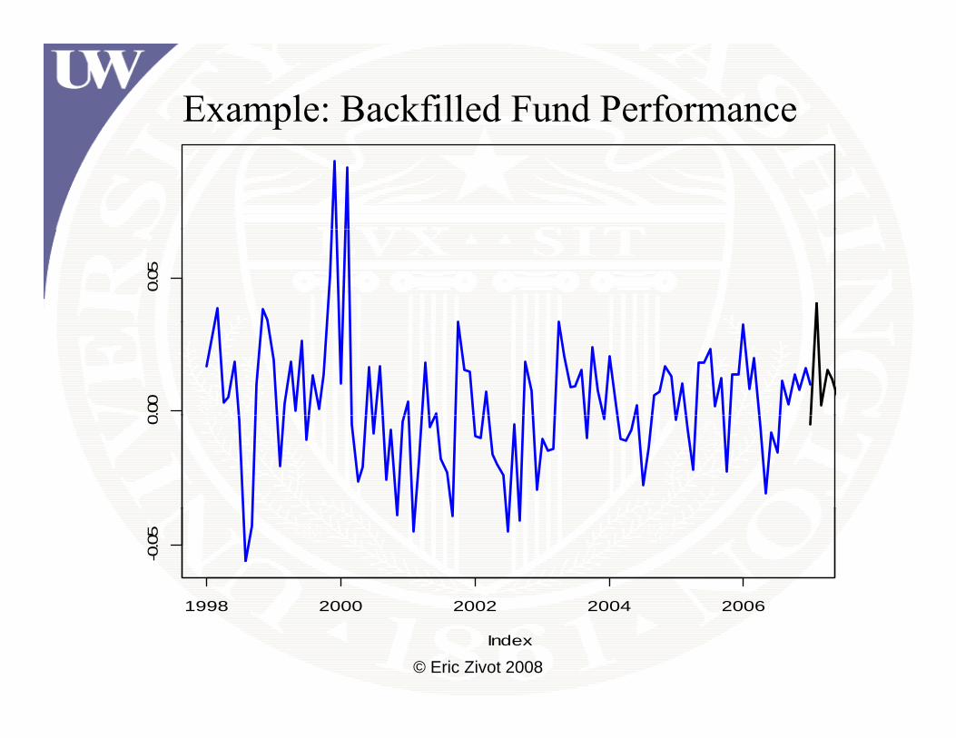
Example: Backfilled Fund Performance0.
050.
000
-0.0
5
1998 2000 2002 2004 2006
© Eric Zivot 2008Index
1998 2000 2002 2004 2006

Example: Simulated portfolio distribution60
% M
odVaR
99%
VaR
4050
99 %
Den
sity
3040
1020
01
© Eric Zivot 2009Returns
-0.08 -0.06 -0.04 -0.02 0.00 0.02 0.04
S-PLUS and S+FinMetrics vs RS PLUS and S+FinMetrics vs R
• Dealing with time series objects in R can beDealing with time series objects in R can be difficult and confusing
timeSeries zoo xts– timeSeries, zoo, xts• Time series regression in R is incompletely
i l t dimplemented– Diagnostic plots, prediction
• R packages give about 80% functional coverage to S+FinMetrics
© Eric Zivot 2009

Some Thoughts About Using R in a C iCorporate Environment
• IT doesn’t want to support itIT doesn t want to support it• Firewalls block R downloads
h ld f l d h• The world runs from an Excel spreadsheet• Analysts with some programming experience
learn R quickly• Not good for the casual userg
© Eric Zivot 2009

ReferencesReferences• Boudt, K., B. Peterson and C. Croux (2008) "Estimation and , , ( )
Decomposition of Downside Risk for Portfolios with Non-Normal Returns," Journal of RiskD d K (2002) M i M k Ri k J h Wil d• Dowd, K. (2002), Measuring Market Risk, John Wiley and Sons
• Goodworth, T. and C. Jones (2007). “Factor-based, Non-Goodwo t , . a d C. Jo es ( 007). acto based, Noparametric Risk Measurement Framework for Hedge Funds and Fund-of-Funds,” The European Journal of Finance.H ll b k J (2003) “D i P f li V l Ri k• Hallerback, J. (2003). “Decomposing Portfolio Value-at-Risk: A General Analysis”, The Journal of Risk 5/2.
• Jorian, P. (2007), Value at Risk, Third Edition, McGraw HillJorian, P. (2007), Value at Risk, Third Edition, McGraw Hill
© Eric Zivot 2009

ReferencesReferences• Jiang, Y. (2009). Overcoming Data Challenges in Fund-of-g, ( ) g g f
Funds Portfolio Management, PhD Thesis, Department of Statistics, University of Washington.L A (2007) H d F d A A l i P i• Lo, A. (2007). Hedge Funds: An Analytic Perspective, Princeton.
• Yamai, Y. and T. Yoshiba (2002). “Comparative Analyses of a a , . a d . os ba ( 00 ). Co pa at ve a yses oExpected Shortfall and Value-at-Risk: Their Estimation Error, Decomposition, and Optimization, Institute for Monetary and Economic Studies Bank of JapanEconomic Studies, Bank of Japan.
© Eric Zivot 2009