using the storm water management model to predict urban

Natural Resource Ecology and Management Publications Natural Resource Ecology and Management

12-3-2013

Using the Storm Water Management Model to predict urban Using the Storm Water Management Model to predict urban

headwater stream hydrological response to climate and land headwater stream hydrological response to climate and land

cover change cover change

J. Y. Wu Iowa State University

Janette R. Thompson Iowa State University, [email protected]

Randy K. Kolka United States Department of Agriculture

Kristie J. Franz Iowa State University, [email protected]

Timothy W. Stewart Iowa State University, [email protected]

Follow this and additional works at: https://lib.dr.iastate.edu/nrem_pubs

Part of the Atmospheric Sciences Commons, and the Natural Resources Management and Policy

Commons

The complete bibliographic information for this item can be found at https://lib.dr.iastate.edu/

nrem_pubs/22. For information on how to cite this item, please visit http://lib.dr.iastate.edu/

howtocite.html.

This Article is brought to you for free and open access by the Natural Resource Ecology and Management at Iowa State University Digital Repository. It has been accepted for inclusion in Natural Resource Ecology and Management Publications by an authorized administrator of Iowa State University Digital Repository. For more information, please contact [email protected].

http://lib.dr.iastate.edu/

http://lib.dr.iastate.edu/

https://lib.dr.iastate.edu/nrem_pubs

https://lib.dr.iastate.edu/nrem_pubs

https://lib.dr.iastate.edu/nrem

https://lib.dr.iastate.edu/nrem_pubs?utm_source=lib.dr.iastate.edu%2Fnrem_pubs%2F22&utm_medium=PDF&utm_campaign=PDFCoverPages

http://network.bepress.com/hgg/discipline/187?utm_source=lib.dr.iastate.edu%2Fnrem_pubs%2F22&utm_medium=PDF&utm_campaign=PDFCoverPages



https://lib.dr.iastate.edu/nrem_pubs/22


http://lib.dr.iastate.edu/howtocite.html

http://lib.dr.iastate.edu/howtocite.html

mailto:[email protected]

Using the Storm Water Management Model to predict urban headwater stream Using the Storm Water Management Model to predict urban headwater stream hydrological response to climate and land cover change hydrological response to climate and land cover change

Abstract Abstract Streams are natural features in urban landscapes that can provide ecosystem services for urban residents. However, urban streams are under increasing pressure caused by multiple anthropogenic impacts, including increases in human population and associated impervious surface area, and accelerated climate change. The ability to anticipate these changes and better understand their effects on streams is important for developing and implementing strategies to mitigate potentially negative effects. In this study, stream flow was monitored during April–November (2011 and 2012), and the data were used to apply the Storm Water Management Model (SWMM) for five urban watersheds in central Iowa, USA, representing a gradient of percent impervious surface (IS, ranging from 5.3 to 37.1%). A set of three scenarios was designed to quantify hydrological responses to independent and combined effects of climate change (18% increase in precipitation), and land cover change (absolute increases between 5.2 and 17.1%, based on separate projections of impervious surfaces for the five watersheds) for the year 2040 compared to a current condition simulation. An additional set of three scenarios examined stream response to different distributions of land cover change within a single watershed. Hydrological responses were quantified using three indices: unit-area peak discharge, flashiness (R-B Index; Richards–Baker Index), and runoff ratio. Stream hydrology was strongly affected by watershed percent IS. For the current condition simulation, values for all three indices were five to seven times greater in the most developed watershed compared to the least developed watershed. The climate change scenario caused a 20.8% increase in unit-area peak discharge on average across the five watersheds compared to the current condition simulation. The land cover change scenario resulted in large increases for all three indices: 49.5% for unit-area peak discharge, 39.3% for R-B Index, and 73.9% for runoff ratio, on average, for the five watersheds. The combined climate and land cover change scenario resulted in slight increases on average for R-B Index (43.7%) and runoff ratio (74.5%) compared to the land cover change scenario, and a substantial increase, on average, in unit area peak discharge (80.1%). The scenarios for different distributions of land cover change within one watershed resulted in changes for all three indices, with an 18.4% increase in unit-area peak discharge for the midstream scenario, and 17.5% (downstream) and 18.1% (midstream) increases in R-B Index, indicating sensitivity to the location of potential additions of IS within a watershed. Given the likelihood of increased precipitation in the future, land use planning and policy tools that limit expansion of impervious surfaces (e.g. by substituting pervious surfaces) or mitigate against their impacts (e.g. by installing bioswales) could be used to minimize negative effects on streams.

Disciplines Disciplines Atmospheric Sciences | Natural Resources Management and Policy

Comments Comments This article is from Hydrology and Earth System Sciences 17 (2013): 4743–4758, doi:10.5194/hess-17-4743-2013.

This article is available at Iowa State University Digital Repository: https://lib.dr.iastate.edu/nrem_pubs/22

http://dx.doi.org/10.5194/hess-17-4743-2013



Hydrol. Earth Syst. Sci., 17, 4743–4758, 2013www.hydrol-earth-syst-sci.net/17/4743/2013/doi:10.5194/hess-17-4743-2013© Author(s) 2013. CC Attribution 3.0 License.

Hydrology and Earth System

SciencesO

pen Access

Using the Storm Water Management Model to predict urbanheadwater stream hydrological response to climateand land cover change

J. Y. Wu1, J. R. Thompson1, R. K. Kolka 2, K. J. Franz3, and T. W. Stewart1

1Department of Natural Resource Ecology and Management, Iowa State University, Ames, IA, USA2Center for Research on Ecosystem Change, USDA Forest Service, Grand Rapids, MN, USA3Department of Geological and Atmospheric Sciences, Iowa State University, Ames, IA, USA

Correspondence to:J. R. Thompson ([email protected])

Received: 15 May 2013 – Published in Hydrol. Earth Syst. Sci. Discuss.: 4 June 2013Revised: 26 August 2013 – Accepted: 27 October 2013 – Published: 3 December 2013

Abstract. Streams are natural features in urban landscapesthat can provide ecosystem services for urban residents.However, urban streams are under increasing pressure causedby multiple anthropogenic impacts, including increases inhuman population and associated impervious surface area,and accelerated climate change. The ability to anticipatethese changes and better understand their effects on streamsis important for developing and implementing strategies tomitigate potentially negative effects. In this study, streamflow was monitored during April–November (2011 and2012), and the data were used to apply the Storm Water Man-agement Model (SWMM) for five urban watersheds in cen-tral Iowa, USA, representing a gradient of percent impervi-ous surface (IS, ranging from 5.3 to 37.1 %). A set of threescenarios was designed to quantify hydrological responses toindependent and combined effects of climate change (18 %increase in precipitation), and land cover change (absoluteincreases between 5.2 and 17.1 %, based on separate projec-tions of impervious surfaces for the five watersheds) for theyear 2040 compared to a current condition simulation. Anadditional set of three scenarios examined stream responseto different distributions of land cover change within a sin-gle watershed. Hydrological responses were quantified us-ing three indices: unit-area peak discharge, flashiness (R−B

Index; Richards–Baker Index), and runoff ratio. Stream hy-drology was strongly affected by watershed percent IS. Forthe current condition simulation, values for all three indiceswere five to seven times greater in the most developed wa-tershed compared to the least developed watershed. The cli-

mate change scenario caused a 20.8 % increase in unit-areapeak discharge on average across the five watersheds com-pared to the current condition simulation. The land coverchange scenario resulted in large increases for all three in-dices: 49.5 % for unit-area peak discharge, 39.3 % forR −B

Index, and 73.9 % for runoff ratio, on average, for the fivewatersheds. The combined climate and land cover changescenario resulted in slight increases on average forR−B In-dex (43.7 %) and runoff ratio (74.5 %) compared to the landcover change scenario, and a substantial increase, on aver-age, in unit area peak discharge (80.1 %). The scenarios fordifferent distributions of land cover change within one water-shed resulted in changes for all three indices, with an 18.4 %increase in unit-area peak discharge for the midstream sce-nario, and 17.5 % (downstream) and 18.1 % (midstream) in-creases inR − B Index, indicating sensitivity to the locationof potential additions of IS within a watershed. Given thelikelihood of increased precipitation in the future, land useplanning and policy tools that limit expansion of impervioussurfaces (e.g. by substituting pervious surfaces) or mitigateagainst their impacts (e.g. by installing bioswales) could beused to minimize negative effects on streams.

1 Introduction

The hydrology of urban streams is responsive to human ac-tivities in the surrounding landscape (Arnold and Gibbons,1996; Walsh et al., 2005; Wenger et al., 2009). Compared

Published by Copernicus Publications on behalf of the European Geosciences Union.

4744 J. Y. Wu et al.: Using SWMM to predict urban headwater stream responses

to streams in more natural settings, urban streams are lo-cated in landscapes associated with less infiltration and moresurface runoff, often leading to greater peak discharge andshorter peak discharge lag times (Anderson, 1970; Arnoldand Gibbons, 1996). Declines in stream water quality andecological condition, such as increases in pollutant and nu-trient concentrations (e.g. Hatt et al., 2004; Pekarova andPekar, 1996), and shifts in organismal assemblages to moreeutrophic species (e.g. Black et al., 2011; Walsh et al., 2001)have commonly been reported for urban streams. Acceler-ated climate change (Denault et al., 2006), land use and landcover change (Grimm et al., 2008), and combinations of suchchanges (Nelson et al., 2009; Tong et al., 2012) are thoughtto be among the major driving factors leading to rapid degra-dation of urban stream systems.

Computer-based hydrological models have been used tobetter understand urban stream responses to potential stres-sors, such as projected changes in climatic conditions andland cover. Frequently used models include the Storm WaterManagement Model (or SWMM; Rossman, 2010; US EPA,2011), the Hydrological Simulation Program-Fortran model(HSPF; Bicknell et al., 1997), and the Soil and Water As-sessment Tool (SWAT; Neitsch et al., 2002), which can beused to predict hydrological responses to user-designed sce-narios at relatively low cost. Of these models, SWMM hasbeen applied in studies of urban streams because of its abil-ity to simulate the hydraulic dynamics of artificial drainagesystems that are prevalent in urban areas (e.g. Denault et al.,2006; Hsu et al., 2000; Meierdiercks et al., 2010). SWMMwas developed to enable appropriate design of drainage sys-tems (e.g. sizing for detention features, evaluating effective-ness of different runoff control strategies) and can be used tosimulate dynamics of single events or for modeling on a con-tinuous basis (US EPA, 2011). The model incorporates pre-cipitation data to simulate surface runoff and pollutant out-puts for sub-catchment areas which are then conveyed to thewatershed outlet by a user-designated drainage system (USEPA, 2011).

Studies using hydrological models to predict stream re-sponse to changes in precipitation amounts and delivery pat-terns have used a variety of techniques to generate future sce-narios (as reviewed by Praskievicz and Chang, 2009). Forexample, in assessments of streamflow responses to climatechange, global climate models (GCMs) and regional climatemodels (RCMs) have been used (e.g. Chang, 2003; Jha etal., 2004; Nelson et al., 2009; Poelmans et al., 2011; Takleet al., 2010; Quilbe et al., 2008). However, the grid scalescommonly used in GCMs (hundreds of km; Boyle, 1998)and RCMs (∼ 50 km; Takle et al., 2010) and their time in-tervals (≥ hourly; Kendon et al., 2012) are not suitable forpredictions at finer spatio-temporal scales. Other approachesthat have been used at more local scales and for shorter timeintervals include linear regression based on historical precip-itation records (Denault et al., 2006; Takle and Herzmann,2010) or projections based on likely proportional changes,

for example,±20 % of current precipitation (Tong et al.,2012).

Similarly, a variety of approaches have been used to createprojections for land cover change, including those based onMarkov-chain probability models that generate both quan-tity and location of additional impervious surfaces (suchas the software packageLand Change Modeler; Eastman,2012, as used by Bowman et al., 2012). Alternatively, logis-tic regression-based methods that incorporate historical landcover analyses combined with socioeconomic (population,land value) driver variables have also been used (Guneralp etal., 2012; Serneels and Lambin, 2001). A third approach thathas been used to predict land cover change is based on sim-ple regression of historical changes in percent of developedland projected to a specified time in the future (Tu, 2009).Unlike the first two methods, land cover change using thethird method is influenced only by the historical land covercharacteristics, such as percent impervious surface (IS).

Some of the previously described prediction methods havebeen applied to investigate hydrological responses to cli-mate change alone (Denault et al., 2006; Jha et al., 2004;Takle et al., 2010), land cover change alone (Meierdierkset al., 2010; Nagy et al., 2012; Rose and Peters, 2001) orto combined climate and land cover changes (e.g. Chen etal., 2005; Choi, 2008; Chung et al., 2011; Cuo et al., 2009;Hamdi et al., 2011; Tong et al., 2012; Yang et al., 2010).In general, these researchers reported greater variability indischarge (flashiness) and greater pollutant loading in re-sponse to increases in IS and/or precipitation. For exam-ple, Chang (2003) used two GCMs (the Canadian Centremodel and Hadley Centre model) to predict climate changein conjunction with an empirical urban growth scenario topredict land cover change for the 2030s in the ConestogaRiver basin in Pennsylvania, USA. Predicted hydrologicalresponses, simulated using the AVGWLF (ArcView Gener-alized Watershed Loading Function) model, indicated a 14 %decrease in mean annual streamflow using the Canadian Cen-tre model versus an 11 % increase using the Hadley Centremodel. Predicted streamflow for the whole basin increased byonly 0.4 % for a 15.5 % increase in urban land area. Chung etal. (2011) investigated an integrated approach using a down-scaling model (SDSM) with HSPF and the Impervious CoverModel (ICM) to predict flow and pollutant concentration inthe Anyangcheon watershed in Korea under three climateconditions and three land use change scenarios. They con-cluded that climate change had greater effects in terms ofincreasing flow rates, and that land cover change had greatereffects in terms of increasing stream water pollutant concen-tration. Poelmans et al. (2011) used statistical downscalingof 58 GCM/RCM runs to predict future climate scenariosand three different urban growth rates to predict outcomesfor the 2050s in a small suburban catchment in the Flanders–Brussels region, Belgium. Their lumped hydrological modelsimulated an 18 % decrease in peak discharge under a pro-jected dry scenario and a 30 % increase in peak discharge

Hydrol. Earth Syst. Sci., 17, 4743–4758, 2013 www.hydrol-earth-syst-sci.net/17/4743/2013/

J. Y. Wu et al.: Using SWMM to predict urban headwater stream responses 4745

under a wet summer scenario. Land cover change scenar-ios predicting increases in developed land ranging from 70to 200 % resulted in increases of peak discharge that rangedfrom 6–16 %.

In a growing number of studies, urban stream responsesto climate and/or land cover change have been examinedfor multiple watersheds. For example, using the AVGWLFmodel, Tu (2009) predicted future climate and land coverchanges and examined responses for streamflow and nitrogenloads at seven study sites in and near Boston, Massachusetts.Model outputs indicated that the greatest impacts from cli-mate and land cover change were related to the seasonal dis-tribution of discharge rate and nitrogen loading in the future,which were projected to be greater in fall and winter andlower in the summer, rather than affecting the average to-tal annual amounts. In another study, Nagy et al. (2012) ob-served hydrological and water quality differences among 13small watersheds located along the Florida Gulf Coast withdifferent watershed percent IS. These researchers reportedincreases in peak flow, flashiness, pH, and specific conduc-tance as impervious surface in the watershed increased (Nagyet al., 2012).

Thus, there is considerable variation in predicted outcomesfor climate change, land cover change, and their potential im-pacts on streams (Praskievicz and Chang, 2009). Previousresearch in the Midwest, however, consistently indicates astrong likelihood of increased storm intensity and total pre-cipitation delivery in this region (Jha et al., 2004; Takle etal., 2010). Further, it has been suggested that small basinsmay experience greater impacts than larger ones (Praskeviczand Chang, 2009). The potential impacts of these changeson small streams in urban areas require additional investiga-tion in order to better elucidate their separate and combinedeffects and to identify appropriate mitigation strategies. Inthe research described in this paper, we examined five wa-tersheds from among 20 small urban headwater streams forwhich we collected water quality and water quantity dataover two years, 2011 and 2012. The five watersheds werepurposefully selected to represent a gradient of percent IS,ranging from 5.3 to 37.1 %. Climate and land cover changewere projected to the year 2040 using regressions based onhistorical data. We then used SWMM to create hydrologicalmodels for these watersheds to answer the following ques-tions:

1. What hydrological differences can be detected amongthe five urban headwater streams along a % IS gradi-ent?

2. What are the hydrological responses to projected cli-mate change, land cover change, and combined climateand land cover change for these stream systems?

3. How might different distributions of land cover changeaffect urban headwater stream hydrology?

2 Methods

2.1 Study area

Five headwater stream watersheds located in Polk County,Iowa, USA, were included in this study (WS1 to WS5;Fig. 1). These watersheds were within the corporate bound-aries of four cities: Altoona, Ankeny, Johnston and Pleas-ant Hill. These cities are located close to Iowa’s state cap-ital (Des Moines), and have experienced rapid populationgrowth in recent years. Between 2000 and 2010, populationsin Altoona, Ankeny, Johnston, and Pleasant Hill increasedby 41 %, 68 %, 100 %, and 73 %, respectively, compared toa 4 % increase for Iowa as a whole (State Data Center ofIowa, 2012). The five watersheds were located within the up-per Midwest climatic region, with average annual precipita-tion over the most recent 25 yr (1987–2011) of 805 mm (Na-tional Climatic Data Center, 2012). About 75 % of annualprecipitation typically occurs between April and September.The watersheds were located along the southern edge of theDes Moines Lobe landform region, a recently glaciated area(14 kyr BP) in which stream network development is ongo-ing. The watersheds were approximately 280 m above sealevel.

Watersheds exhibited variation in size, initial percent IS,and average slope (Table 1). Two of the watersheds (WS1 andWS2) were located in Pleasant Hill (Fig. 1). Land cover inWS1 included residential development (clustered in the up-stream area), agricultural land (midstream area), and pastureland (downstream area). The second watershed (WS2) con-tained a segment of US Highway 65 and was otherwise dom-inated by agricultural and forested areas. The third watershed(WS3) was in northeastern Altoona, along the eastern bound-ary of the city, and it contained residential, commercial, andagricultural land. The fourth watershed (WS4) was located inJohnston, and the fifth (WS5) was in Ankeny. Both WS4 andWS5 contained primarily residential areas. Although theirdrainage densities were similar, WS4 was characterized bya lower % IS than WS5.

2.2 Stream monitoring methods and other data sources

Flow rates were measured twice per month from Aprilto October at defined channel cross sections near eachstream outlet using a FLO-MATE 2000 Water Current andFlowmeter™ (Hach Company, Loveland, CO). Dischargewas then determined using the cross-section method ofRantz (1982). Area of the defined channel cross section wasdetermined by measuring stream depth at evenly distributedpoints (varying from one to seven) and multiplying by width.The maximum distance between adjacent measuring pointswas 0.5 m.

In addition, stream stage was continuously recorded at5 min intervals from mid-May to October at each crosssection using HOBO U20 water level data loggers (Onset

www.hydrol-earth-syst-sci.net/17/4743/2013/ Hydrol. Earth Syst. Sci., 17, 4743–4758, 2013


32

1

2 3

4

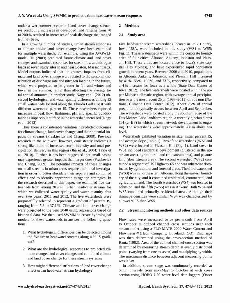
Fig. 1. Five headwater stream watersheds located in four cities (one each in Altoona, Ankeny, and 5 Johnston, and two in Pleasant Hill) in Polk County, central Iowa. Shaded areas represent impervious 6 surface in 2011, watershed boundaries for WS1 through WS5 are outlined with red lines. 7 8

9

Fig. 1.Five headwater stream watersheds located in four cities (one each in Altoona, Ankeny, and Johnston, and two in Pleasant Hill) in PolkCounty, central Iowa. Shaded areas represent impervious surface in 2011, watershed boundaries for WS1 through WS5 are outlined with redlines.

Table 1. Geographic characteristics, drainage density, distance to nearest weather station, and projected percent impervious surface (IS,2040) for five urban watersheds (WS1 to WS5) in central Iowa representing a percent impervious surface gradient. Total drainage density isthe sum of road gutter, storm sewer and surface channel densities.

WS1 WS2 WS3 WS4 WS5

Area (ha) 194.9 61.8 269.8 89.5 92.0Current percent IS 5.3 8.0 18.2 28.3 37.1Average slope (%) 10.3 5.4 5.6 10.5 8.8Total drainage density (km km−2) 3.2 10.7 5.1 9.0 8.8Road gutter density (km km−2) – – 0.6 0.3 0.3Storm sewer density (km km−2) 0.2 – 1.3 6.7 6.5Surface channel density (km km−2) 3.0 10.7 3.3 2.0 1.9Distance to nearest weather station (km) 10.4 5.8 15.0 5.3 3.1

Land cover projectionPercent IS in 2040 10.5 15.7 35.3 45.0 45.0Absolute change (%) 5.2 7.8 17.1 16.7 7.9Relative change (%) 97.6 97.7 93.7 59.1 21.2

Computer Corporation, Inc., Pocasset, MA). An additionaldata logger was used to measure barometric pressure for cor-rection of stream stage data. Continuous stage data were con-verted to discharge using a stage-discharge rating curve de-veloped for each stream.

Digital elevation models (DEMs) at one-meter resolutionwere generated from light detection and ranging (lidar) dataavailable from the Iowa LiDAR Mapping Project (GeoTREE,2011). Impervious surface cover for each watershed wasmanually digitized based on 2011 aerial photo images. Storm

sewer GIS layers were obtained from staff members in thefour cities. Five-minute interval precipitation data were ob-tained from Iowa SchoolNet system (Iowa EnvironmentalMesonet, 2012). Three weather stations were selected basedon proximity to the five watersheds, “SDRI4” in Des Moines(for WS1, WS2, and WS3), “SGRI4” in Johnston (for WS4),and “SAKI4” in Ankeny (for WS5).



2.3 Calibration and validation of the StormWater Management Model

The Storm Water Management Model (SWMM Version5.0.022; Rossman, 2010; US EPA, 2011) was used tosimulate current and projected watershed conditions. Sub-catchments were delineated to collect precipitation, and thekinematic wave method (Rossman, 2010) was used to routewater through designated channels or pipes. Individual mod-els were constructed for each of the five watersheds using5 min interval precipitation data to simulate surface runoffand channelized discharge in road gutters, storm sewers, andsurface channels. The embedded groundwater module wasactivated for all models using the same precipitation event(6.4 mm delivered to each watershed 5 h before each simula-tion) to “recharge” groundwater. Because we were interestedin flow dynamics associated with single precipitation events,the effects of evaporation were not included (Gironás et al.,2009). Infiltration processes were simulated using Horton’sequation within the model (Green, 1986).

Model parameters were obtained in three different ways.The first set of parameters were defined based on existingdata for sub-catchment and drainage structure parameters,% IS, and slope. The second set of parameters were cali-brated using available discharge observations, sub-catchmentwidth, coefficients for groundwater equations, and Man-ning’s roughness coefficient (n) for impervious surfaces, per-vious surfaces, and channels. All other parameters were setto default values or values suggested by the SWMM appli-cation manual (Gironás et al., 2009). For example, the initialinfiltration rate was 100 mm h−1, the constant infiltration ratewas 7 mm h−1, and the decay constant was 3.5 for Horton’sinfiltration equation.

Precipitation events (26 June 2011) recorded at the threeweather stations were chosen to use for the calibration pro-cess. Precipitation depths were 8.9 mm (WS1, WS2, andWS3), 10.4 mm (WS4), and 12.7 mm (WS5). The modelswere then manually calibrated for best fit to the continu-ous discharge data derived from field monitoring for thesame events. Precipitation events from the three weather sta-tions on another date (25 May 2011) were used to validatethe models. Precipitation depths for the validation procedurewere 21.3 mm (WS1, WS2, and WS3), and 23.1 mm (WS4and WS5).

Model performance was quantified using the coefficient ofdetermination (R2) and Nash–Sutcliffe model efficiency co-efficient (NSE). The coefficient of determination ranges from0 to 1, where greater values indicate a closer relationship be-tween predicted and observed values for discharge. The NSEstatistic has a range of -∞ to 1. A greater value indicates abetter prediction of discharge, shown in Eq. (1):

NSE= 1−

∑(Qo,t − Qm,t)

2∑(Qo,t − Qo)2

, (1)

where NSE is the Nash–Sutcliffe model efficiency coeffi-cient,Qo,t is the observed discharge (m3 s−1) at timet , Qm,tis the modeled discharge (m3 s−1) at timet , and is the aver-age for the observed discharge (m3 s−1).

2.4 Climate change projection

Our projections for climate change were based solely onchanges in precipitation quantities delivered to each water-shed. A precipitation event occurring on 10 June 2011 wasused as the current climate condition for all five watersheds.This event delivered 16.8 mm of precipitation in one hour,representing a 1 h, 2-month recurrence interval event in thisregion. We chose this event because it represents a commonprecipitation event, would not be likely to induce flooding(which would preclude estimates of response variables thatdescribe flow dynamics within the channel), and was inter-mediate between the calibration (approximately 11 mm) andvalidation (approximately 22 mm) events, reducing some ofthe uncertainty associated with the hydrological projections.We based our projection on a simple linear regression model,and we do not assume that precipitation increases would nec-essarily be uniform throughout the year, but we have usedthe general projection to create a single hypothetical futureevent. Further, although other methods could be used to gen-erate future precipitation scenarios, the spatio-temporal res-olution of even regional climate downscaling models is rela-tively coarse for application at headwater stream/single eventscales. To create a future (2040) precipitation event, annualprecipitation for the region was obtained for the period 1895to 2011 (National Climatic Data Center, 2012). Using linearregression (similar to method of Denault et al., 2006; Takleand Herzmann, 2010), annual precipitation in 2040 was pro-jected to be 18 % more than it was during 2011. This pro-portional increase is consistent with results reported for thisregion of study by previous researchers (e.g. Jha et al., 2004;Takle et al., 2010). The projected precipitation event was de-signed to have the same duration and time distribution as theprecipitation event on 10 June 2011.

2.5 Land cover change projection

Our assessment of future land cover change impacts wasbased solely on predicted changes in impervious surfacecover in each of the study watersheds. Percent IS in 2011,calculated by dividing IS area within each watershed by thecorresponding total watershed area, was used as the currentland cover condition (again using the current condition 10June 2011 rainfall event). Land cover was projected to theyear 2040 using separate regression models based on quan-tification of total IS areas for each of the four cities (Al-toona, Ankeny, Johnston, and Pleasant Hill) in 1940, 1961,1990, 2002, and 2011 (method adapted from Tu, 2009). Bi-nomial curves provided the best fit for the four cities, withcoefficients of determination (R2) of 0.997 (Altoona), 0.984



(Ankeny), 0.973 (Johnston), and 0.994 (Pleasant Hill). Theincrease of IS area within each watershed (Table 1) was as-sumed to be the same as that for each city, unless the pro-jected % IS for the watershed exceeded 45 % (which we setas a maximum according to the % IS for other fully devel-oped residential areas in our study area). We used a semi-distributed approach to increase percent impervious surfaceby the projected amount within each sub-catchment of eachwatershed by adjusting the values for each of them in the in-put file for each model. We did not change the amount or dis-tribution of storm sewer infrastructure for this analysis. Forthe land cover change simulation that included all five wa-tersheds, increases in IS area were evenly distributed acrosseach watershed.

2.6 SWMM simulations with independent andcombined effects of climate and land cover change

We conducted current condition SWMM simulations usinga single precipitation event (10 June 2011, 16.8 mm precip-itation in one hour) and 2011 land cover data in all of thecalibrated SWMM models (Table 2). A set of three differentclimate and land cover change scenarios were designed forthis part of the study. In the first scenario, we used a precip-itation event projected for 2040 with actual 2011 land cover.In the second scenario, we used the actual 2011 precipita-tion events and the projected land cover for 2040. In the thirdscenario, we used 2040 projections for both climate and landcover.

2.7 SWMM simulations with different distributionsof land cover change in a single watershed

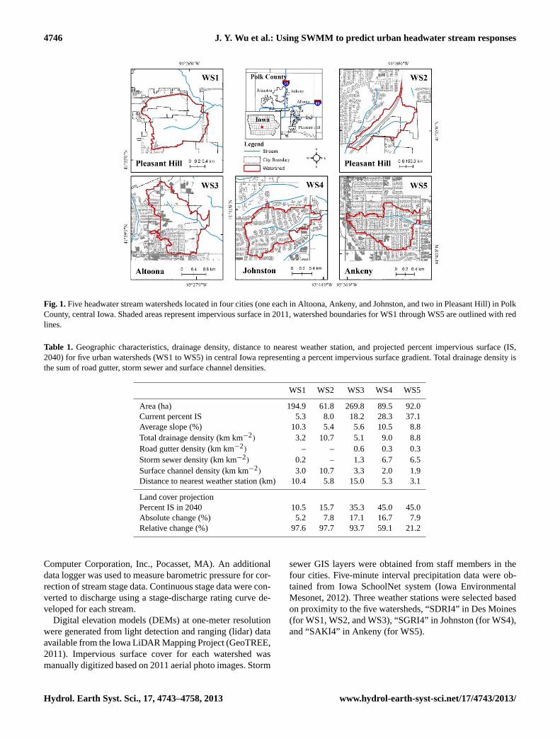
To assess effects of different distributions of future landcover changes, one watershed (WS4) was divided into threesections (Fig. 2). We chose WS4 because it initially hadevenly distributed IS and was projected to have a relativelylarge IS increase. The three sections were downstream, mid-stream, and upstream areas within the watershed, and char-acterized by similar size and initial % IS (2011). In this wa-tershed, existing impervious surfaces (2011) were relativelyevenly distributed between 10 % and 95 % distances to thewatershed outlet. The same increase in urban land cover (tocause a 16.7 % absolute increase for each section) was ap-plied within one of the three sections, changing the impervi-ous surface distribution from upstream to downstream. Theprojected precipitation event for 2040 in WS4 was used foreach simulation in this set of scenarios.

2.8 Quantifying hydrological indices

To quantify hydrological responses, three indices were calcu-lated for current condition and scenario simulations, includ-ing unit-area peak discharge, Richards-Baker Index (here-afterR−B Index; Baker et al., 2004), and runoff ratio. Unit-area peak discharge is the quotient of peak discharge divided

by watershed area, and indicates the greatest amount of dis-charge generated by a unit area in a single precipitation event.A greater value of peak discharge indicates greater potentialfor flooding (Huong and Pathirana, 2013). TheR − B Indexmeasures oscillations in discharge relative to total discharge,also referred to as “flashiness”. A higher value of theR − B

Index indicates a greater difference between high and lowflows, which may be linked to changes in channel morphol-ogy, water quality and habitat structure of stream ecosystems(Shields et al., 2010; Violin et al., 2011). We calculated theR − B Index based on 5 min interval discharge data, as perEq. (2):

R-B Index=

∑ni=1 |qi − qi−1|∑n

i=1qi

, (2)

wheren is the total number of discharge records, andqi is thei th measured discharge of a stream, andqi−1 is thei − 1 thmeasured discharge of a stream.

The runoff ratio is the total discharge depth divided bytotal precipitation depth, which indicates the proportion ofprecipitation that is discharged in surface channels. A highervalue of runoff ratio indicates an increase of surface runoffand may result in decreases in groundwater level because ofless infiltration (Foster and Chilton, 2004).

2.9 Evaluation of model uncertainty

Because we manually calibrated the models, we also an-alyzed uncertainty associated with three of the model in-put parameters, by varying sub-catchment width by±10 %(Gironas et al., 2009), and by varying Manning’sn to test twoplausible end values for pervious surfaces (0.2 and 0.5) andnatural channels (0.04 and 0.055) (Chow, 1959). We chosethese parameters because they were likely to have the great-est impact on simulated discharge events during the manualcalibration process. Given that SWMM is run through a GUI,extensive analyses were not practical, so we assessed onewatershed (WS 4, which was used in the largest number ofscenarios) and tested uncertainty by changing one of theseparameters at a time while holding all others constant. Weused unit-area peak discharge to measure changes in modelresults, andR2 and NSE to evaluate model performance aswe did for calibration and validation.

3 Results

3.1 Calibration and validation of the StormWater Management Model

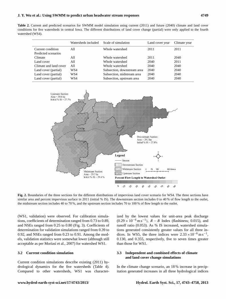
Calibrated model parameters (Table 3) were used to generatehydrographs for each watershed (Fig. 3). Generally, calibra-tion and validation hydrographs demonstrated acceptable fitbetween observed and simulated discharge, although somedifferences in timing (WS5, calibration) and/or magnitude



Table 2. Current and predicted scenarios for SWMM model simulation using current (2011) and future (2040) climate and land coverconditions for five watersheds in central Iowa. The different distributions of land cover change (partial) were only applied to the fourthwatershed (WS4).

Watersheds included Scale of simulation Land cover year Climate year

Current condition All Whole watershed 2011 2011Predicted scenariosClimate All Whole watershed 2011 2040Land cover All Whole watershed 2040 2011Climate and land cover All Whole watershed 2040 2040Land cover (partial) WS4 Subsection, downstream area 2040 2040Land cover (partial) WS4 Subsection, midstream area 2040 2040Land cover (partial) WS4 Subsection, upstream area 2040 2040

33

1

2

Fig. 2. Boundaries of the three sections for the different distributions of impervious land cover 3 scenario for WS4. The three sections have similar area and percent impervious surface in 2011 4 (initial % IS). The downstream section includes 0 to 40% of flow length to the outlet, the 5 midstream section includes 40 to 70%, and the upstream section includes 70 to 100% of flow 6 length to the outlet. 7

8

Fig. 2. Boundaries of the three sections for the different distributions of impervious land cover scenario for WS4. The three sections havesimilar area and percent impervious surface in 2011 (initial % IS). The downstream section includes 0 to 40 % of flow length to the outlet,the midstream section includes 40 to 70 %, and the upstream section includes 70 to 100 % of flow length to the outlet.

(WS1, validation) were observed. For calibration simula-tions, coefficients of determination ranged from 0.73 to 0.89,and NSEs ranged from 0.25 to 0.80 (Fig. 3). Coefficients ofdetermination for validation simulations ranged from 0.39 to0.92, and NSEs ranged from 0.23 to 0.91. Among the mod-els, validation statistics were somewhat lower (although stillacceptable as per Moriasi et al., 2007) for watershed WS1.

3.2 Current condition simulation

Current condition simulations describe existing (2011) hy-drological dynamics for the five watersheds (Table 4).Compared to other watersheds, WS1 was character-

ized by the lowest values for unit-area peak discharge(0.29× 10−6 m s−1), R − B Index (flashiness; 0.015), andrunoff ratio (0.053). As % IS increased, watershed simula-tions generated consistently greater values for all three in-dices. In WS5, the three indices were 2.33×10−6 m s−1,0.130, and 0.355, respectively, five to seven times greaterthan those for WS1.

3.3 Independent and combined effects of climateand land cover change simulations

In the climate change scenario, an 18 % increase in precip-itation generated increases in all three hydrological indices



34

1

2

Fig. 3. Hydrograph segments for calibration (left column) and validation (right column) of the 3 five models (WS1 to WS5). Discharge was standardized by watershed area. 4

5

6

Fig. 3. Hydrograph segments for calibration (left column) and validation (right column) of the five models (WS1 to WS5). Discharge wasstandardized by watershed area.

Table 3. Calibrated SWMM model parameters for five watersheds (WS1 to WS5) in central Iowa. A1, B1, A2, and B2 are coefficients forthe groundwater equation in SWMM.

Parameters and Statistics WS1 WS2 WS3 WS4 WS5

Number of sub-catchments 29 32 49 52 60Average width of sub-catchments (m) 704 259 324 101 123Manning’sn (impervious surfaces) 0.017 0.05 0.05 0.05 0.05Manning’sn (pervious surfaces) 0.18 0.5 0.2 0.4 0.4Manning’sn (channels: natural) 0.05 0.05 0.04 0.05 0.04Manning’sn (channels: storm sewer) – – 0.012 0.012 0.012Manning’sn (channels: gutter) 0.015 – 0.015 0.015 0.015Parameters for groundwater equationA1 0.0005 0.050 0.0070 0.050 0.008B1 1.00 1.00 2.00 1.00 1.00A2 0.0005 0.007 0.0010 0.050 0.008B2 1.00 1.00 1.00 1.00 1.00



Table 4. Hydrological response characteristics for current condition, climate change, land cover change, and combined scenarios for fivewatersheds (WS1 to WS5) in central Iowa. The relative changes in percent for climate, land cover and combined scenarios are calculatedcompared to the current condition.

Scenarios Indices WS1 WS2 WS3 WS4 WS5

Current conditionUnit-area peak discharge (×10−6 m s−1) 0.29 0.88 1.37 1.62 2.33R − B Index 0.015 0.027 0.060 0.061 0.130Runoff ratio 0.053 0.077 0.181 0.266 0.355

Climate

Unit-area peak discharge (×10−6 m s−1) 0.35 1.02 1.69 1.97 2.82Change (%) 21.1 16.8 23.4 21.8 21.1R − B Index 0.015 0.027 0.061 0.066 0.136Change (%) 1.7 2.0 2.0 8.3 4.7Runoff ratio 0.053 0.077 0.181 0.268 0.358Change (%) 0.0 0.6 0.1 0.7 0.7

Land cover


Climate and land cover


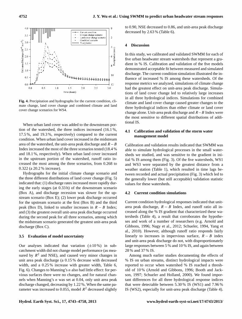
compared to the current condition (e.g. Fig. 4 for WS4).Specifically, unit-area peak discharge for the five watershedsranged from 0.35× 10−6 m s−1 to 2.82× 10−6 m s−1, an in-crease of 20.8 % on average compared to current conditionvalues (Table 4). The change in unit-area peak dischargewas greatest in WS3 (23.4 %). Increases inR − B Index andrunoff ratio compared to current condition values were muchsmaller than those for unit-area peak discharge. On aver-age, theR − B Index increased 3.7 %, ranging from 0.015to 0.136, with the greatest proportional increase occurringin WS4 (8.3 %). Watersheds with higher % IS generally hadgreater values forR −B Index. Runoff ratio increased 0.4 %on average, ranging from 0.053 to 0.358, with the greatestproportional increases occurring in WS4 and WS5 (0.7 %).

A separate analysis (data not shown) of responses for thethree indices in WS1 and WS4 to the storm event in the vali-dation model (21.3–23.1 mm precipitation) indicated consis-tent trajectories of change for all three indices at both levelsof initial IS beyond that tested in the climate change scenario(e.g. the precipitation gradient from 16.8 mm (current condi-tion) to 19.8 mm (climate change scenario) and 23.1 mm forthe validation scenario). The land cover change scenario ledto a greater hydrological response compared to the currentcondition than did the climate change scenario (e.g. Fig. 4for WS4). All three response indices increased to a greaterdegree than they did in the climate change scenario (Table 4).Unit-area peak discharge ranged from 0.58 to 2.80 (an aver-age increase of 49.5 %). The greatest increase compared tothe current condition (99.7 %) occurred in WS1. Increases in

theR−B Index ranged from 0.019 to 0.148, with an averageincrease of 39.3 %. The greatest increase (68.4 %) occurredin WS3. Runoff ratio ranged from 0.105 to 0.430, a 73.9 %average increase, with the greatest increase (97.9 %) detectedfor WS2.

The combined effects of climate and land cover changesgenerated the largest changes in the hydrograph (e.g. Fig. 4for WS4) and for all three indices (Table 4). Unit-area peakdischarge increased from 0.69 to 3.40, with an average in-crease of 80.1 %. The greatest increase (138.0 %) occurredin WS1. TheR−B Index ranged from 0.019 to 0.156 (an av-erage increase of 43.7 %), with the largest increase (66.9 %)in WS3. The runoff ratio ranged from 0.105 to 0.433 (an av-erage increase of 74.5 %), with the largest increase (98.9 %)in WS2.

3.4 Simulations of different distributions of land coverchange for WS4

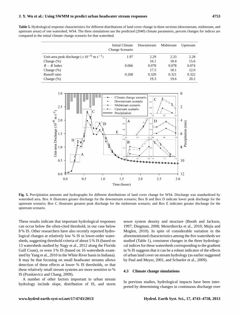
For different distributions of land cover change in WS4, weobserved consistent increases but different patterns of changefor each of the hydrological indices (Table 5). The unit-areapeak discharge responded most strongly to additional % ISin the midstream area, increasing by 18.4 %, compared tothe other two scenarios (16.1 % and 15.6 %; Table 5). Theresponse of theR − B Index to greater % IS in the upstreamarea was much lower (12.0 %) compared to the other two sce-narios (17.5 % and 18.1 %). Increases in runoff ratios weresimilar for the three scenarios (ranging from 19.3 to 20.2 %;Table 5).



35

1

2

3

Fig. 4. Precipitation and hydrographs for the current condition, climate change, land cover change 4 and combined climate and land cover change scenarios for WS4. 5

6

Fig. 4. Precipitation and hydrographs for the current condition, cli-mate change, land cover change and combined climate and landcover change scenarios for WS4.

When urban land cover was added to the downstream por-tion of the watershed, the three indices increased (16.1 %,17.5 %, and 19.3 %, respectively) compared to the currentcondition. When urban land cover increased in the midstreamarea of the watershed, the unit-area peak discharge andR−B

Index increased the most of the three scenarios tested (18.4 %and 18.1 %, respectively). When urban land cover increasedin the upstream portion of the watershed, runoff ratio in-creased the most among the three scenarios, from 0.268 to0.322 (a 20.2 % increase).

Hydrographs for the initial climate change scenario andthe three different distributions of land cover change (Fig. 5)indicated that: (1) discharge rates increased more rapidly dur-ing the early stages (at 0.33 h) of the downstream scenario(Box A), and discharge recession was slower for the up-stream scenario (Box E); (2) lower peak discharge occurredfor the upstream scenario at the first (Box B) and the thirdpeak (Box D), linked to smaller increases inR − B Index;and (3) the greatest overall unit-area peak discharge occurredduring the second peak for all three scenarios, among whichthe midstream scenario generated the greatest unit-area peakdischarge (Box C).

3.5 Evaluation of model uncertainty

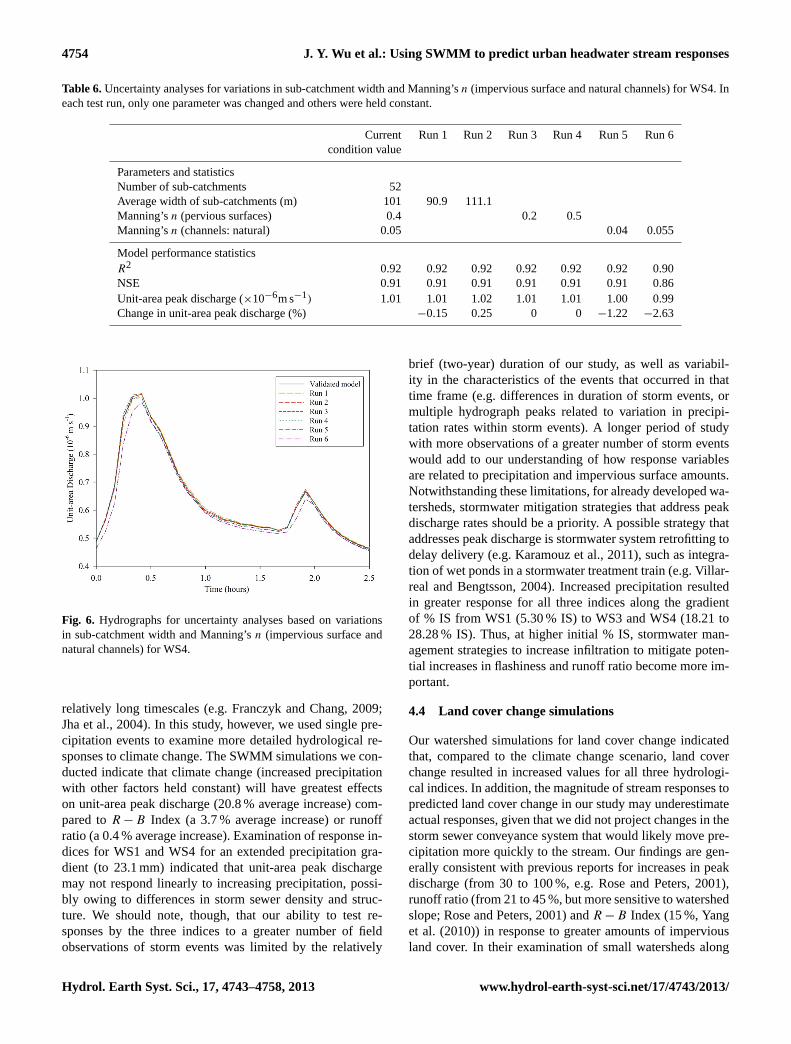
Our analyses indicated that variation (±10 %) in sub-catchment width did not change model performance (as mea-sured byR2 and NSE), and caused very minor changes inunit area peak discharge (a 0.15 % decrease with decreasedwidth, and a 0.25 % increase with greater width, Table 6,Fig. 6). Changes to Manning’sn also had little effect: for per-vious surfaces there were no changes, and for natural chan-nels when Manning’sn was set at 0.04, only unit area peakdischarge changed, decreasing by 1.22 %. When the same pa-rameter was increased to 0.055, modelR2 decreased slightly

to 0.90, NSE decreased to 0.86, and unit-area peak dischargedecreased by 2.63 % (Table 6).

4 Discussion

In this study, we calibrated and validated SWMM for each offive urban headwater stream watersheds that represent a gra-dient in % IS. Calibration and validation of the five modelsdemonstrated acceptable fit between measured and simulateddischarge. The current condition simulation illustrated the in-fluence of increased % IS among these watersheds. Of theresponse metrics we analyzed, simulations of climate changehad the greatest effect on unit-area peak discharge. Simula-tions of land cover change led to relatively large increasesin all three hydrological indices. Simulations for combinedclimate and land cover change caused greater changes to thethree hydrological indices than either climate or land coverchange alone. Unit-area peak discharge andR−B Index werethe most sensitive to different spatial distributions of addi-tional IS.

4.1 Calibration and validation of the storm watermanagement model

Calibration and validation results indicated that SWMM wasable to simulate hydrological processes in the small water-sheds we studied, and was sensitive to the gradient in ini-tial % IS among them (Fig. 3). Of the five watersheds, WS1and WS3 were separated by the greatest distance from aweather station (Table 1), which resulted in time lags be-tween recorded and actual precipitation (Fig. 3) which led tothe generally lower (but still acceptable) validation statisticvalues for these watersheds.

4.2 Current condition simulations

Current condition hydrological responses indicated that unit-area peak discharge,R − B Index, and runoff ratio all in-creased along the % IS gradient that characterized these wa-tersheds (Table 4), a result that corroborates the hypothe-ses and work of a number of researchers (e.g. Arnold andGibbons, 1996; Nagy et al., 2012; Schueler, 1994, Yang etal., 2010). However, although runoff ratio responds fairlylinearly to increases in impervious surface,R − B indexand unit-area peak discharge do not, with disproportionatelylarge responses between 5 % and 10 % IS, and again between28 % and 37 % IS.

Among much earlier studies documenting the effects of% IS on urban streams, distinct hydrological impacts werereported to occur when watershed % IS reached a thresh-old of 10 % (Arnold and Gibbons, 1996; Booth and Jack-son, 1997; Schueler and Holland, 2000). We found impor-tant differences for all three hydrological response indicesthat were detectable between 5.30 % IS (WS1) and 7.96 %IS (WS2), especially for unit-area peak discharge (Table 4).



Table 5.Hydrological response characteristics for different distributions of land cover change in three sections (downstream, midstream, andupstream areas) of one watershed, WS4. The three simulations use the predicted (2040) climate parameters, percent changes for indices arecompared to the initial climate change scenario for that watershed.

Initial Climate Downstream Midstream UpstreamChange Scenario

Unit-area peak discharge (×10−6 m s−1) 1.97 2.29 2.33 2.28Change (%) 16.1 18.4 15.6R − B Index 0.066 0.078 0.078 0.074Change (%) 17.5 18.1 12.0Runoff ratio 0.268 0.320 0.321 0.322Change (%) 19.3 19.6 20.2

36

1

2

Fig. 5. Precipitation amounts and hydrographs for different distributions of land cover change for 3 WS4. Discharge was standardized by watershed area. Box A illustrates greater discharge for the 4 downstream scenario; Box B and Box D indicate lower peak discharge for the upstream scenario; 5 Box C illustrates greatest peak discharge for the midstream scenario; and Box E indicates greater 6 discharge for the upstream scenario. 7

8

Fig. 5. Precipitation amounts and hydrographs for different distributions of land cover change for WS4. Discharge was standardized bywatershed area. Box A illustrates greater discharge for the downstream scenario; Box B and Box D indicate lower peak discharge for theupstream scenario; Box C illustrates greatest peak discharge for the midstream scenario; and Box E indicates greater discharge for theupstream scenario.

These results indicate that important hydrological responsescan occur below the often-cited threshold, in our case below8 % IS. Other researchers have also recently reported hydro-logical changes at relatively low % IS in lower-order water-sheds, suggesting threshold criteria of about 5 % IS (based on13 watersheds studied by Nagy et al., 2012 along the FloridaGulf Coast), or even 3 % IS (based on 16 watersheds exam-ined by Yang et al., 2010 in the White River basin in Indiana).It may be that focusing on small headwater streams allowsdetection of these effects at lower % IS thresholds, or thatthese relatively small stream systems are more sensitive to %IS (Praskievicz and Chang, 2009).

A number of other factors important to urban streamhydrology include slope, distribution of IS, and storm

sewer system density and structure (Booth and Jackson,1997; Dingman, 2008; Meierdiercks et al., 2010; Mejia andMoglen, 2010). In spite of considerable variation in theaforementioned characteristics among the five watersheds westudied (Table 1), consistent changes in the three hydrologi-cal indices for these watersheds corresponding to the gradientin % IS suggests that it can be a robust indicator of the effectsof urban land cover on stream hydrology (as earlier suggestedby Paul and Meyer, 2001, and Schueler et al., 2009).

4.3 Climate change simulations

In previous studies, hydrological impacts have been inter-preted by determining changes in continuous discharge over



Table 6.Uncertainty analyses for variations in sub-catchment width and Manning’sn (impervious surface and natural channels) for WS4. Ineach test run, only one parameter was changed and others were held constant.

Current Run 1 Run 2 Run 3 Run 4 Run 5 Run 6condition value

Parameters and statisticsNumber of sub-catchments 52Average width of sub-catchments (m) 101 90.9 111.1Manning’sn (pervious surfaces) 0.4 0.2 0.5Manning’sn (channels: natural) 0.05 0.04 0.055

Model performance statisticsR2 0.92 0.92 0.92 0.92 0.92 0.92 0.90NSE 0.91 0.91 0.91 0.91 0.91 0.91 0.86Unit-area peak discharge (×10−6m s−1) 1.01 1.01 1.02 1.01 1.01 1.00 0.99Change in unit-area peak discharge (%) −0.15 0.25 0 0 −1.22 −2.63

37

1

2

3

Fig. 6. Hydrographs for uncertainty analyses based on variations in sub-catchment width and 4 Manning’s n (impervious surface and natural channels) for WS4. 5

6

Fig. 6. Hydrographs for uncertainty analyses based on variationsin sub-catchment width and Manning’sn (impervious surface andnatural channels) for WS4.

relatively long timescales (e.g. Franczyk and Chang, 2009;Jha et al., 2004). In this study, however, we used single pre-cipitation events to examine more detailed hydrological re-sponses to climate change. The SWMM simulations we con-ducted indicate that climate change (increased precipitationwith other factors held constant) will have greatest effectson unit-area peak discharge (20.8 % average increase) com-pared toR − B Index (a 3.7 % average increase) or runoffratio (a 0.4 % average increase). Examination of response in-dices for WS1 and WS4 for an extended precipitation gra-dient (to 23.1 mm) indicated that unit-area peak dischargemay not respond linearly to increasing precipitation, possi-bly owing to differences in storm sewer density and struc-ture. We should note, though, that our ability to test re-sponses by the three indices to a greater number of fieldobservations of storm events was limited by the relatively

brief (two-year) duration of our study, as well as variabil-ity in the characteristics of the events that occurred in thattime frame (e.g. differences in duration of storm events, ormultiple hydrograph peaks related to variation in precipi-tation rates within storm events). A longer period of studywith more observations of a greater number of storm eventswould add to our understanding of how response variablesare related to precipitation and impervious surface amounts.Notwithstanding these limitations, for already developed wa-tersheds, stormwater mitigation strategies that address peakdischarge rates should be a priority. A possible strategy thataddresses peak discharge is stormwater system retrofitting todelay delivery (e.g. Karamouz et al., 2011), such as integra-tion of wet ponds in a stormwater treatment train (e.g. Villar-real and Bengtsson, 2004). Increased precipitation resultedin greater response for all three indices along the gradientof % IS from WS1 (5.30 % IS) to WS3 and WS4 (18.21 to28.28 % IS). Thus, at higher initial % IS, stormwater man-agement strategies to increase infiltration to mitigate poten-tial increases in flashiness and runoff ratio become more im-portant.

4.4 Land cover change simulations

Our watershed simulations for land cover change indicatedthat, compared to the climate change scenario, land coverchange resulted in increased values for all three hydrologi-cal indices. In addition, the magnitude of stream responses topredicted land cover change in our study may underestimateactual responses, given that we did not project changes in thestorm sewer conveyance system that would likely move pre-cipitation more quickly to the stream. Our findings are gen-erally consistent with previous reports for increases in peakdischarge (from 30 to 100 %, e.g. Rose and Peters, 2001),runoff ratio (from 21 to 45 %, but more sensitive to watershedslope; Rose and Peters, 2001) andR − B Index (15 %, Yanget al. (2010)) in response to greater amounts of imperviousland cover. In their examination of small watersheds along



the Gulf Coast, Nagy et al. (2012) reported greater effects ofincreasing % IS on peak discharge, but lesser effects onR−B

Index. It is likely that the relative importance of changes inclimate and land cover on stream hydrology are subject to thespecifics of scenario designs (e.g. differing interpretations of-fered by Hamdi et al., 2011; Tong et al. 2012; Tu, 2009).Notwithstanding, our land cover change simulations providefurther support for the contention that important hydrologicalchanges occur at thresholds below 10 % IS, based on consis-tent increases in all three response indices for the predictedimpervious surface change from 5.30 to 10.47 % in WS1 andfrom 7.96 to 15.74 % in WS2.

4.5 Combined climate and land coverchange simulations

The combined climate and land cover change simulations ledto changes in response indices that were slightly greater thanadditive effects for climate and land cover change consid-ered independently (Table 4). Further, hydrographs for WS4(Fig. 4) indicate that runoff volume increases for each predic-tive scenario, most significantly for the combined effects ofclimate and land cover change. Although previous work hasdocumented additive effects of combined climate and landcover changes (e.g. Nelson et al., 2009; Tong et al., 2012; Tu,2009), conclusions about which influence might be stronger(either climate or land cover change) have been inconsistent,possibly owing to differences in prediction methods and themagnitude of relative changes in the projections used to makethe predictions (Chang, 2003; Chen et al., 2005; Cuo et al.,2009; Davis Todd et al., 2007; Tang et al., 2005). For ex-ample, Tong et al. (2012) reported that climate change (as-suming a 2 % increase in temperature, and 20 % increase inprecipitation) led to a greater change in mean daily flow thandid land cover change when both were projected to 2050.However, when their climate change assumption was altered(to a 4 % increase in temperature with associated increasesin evaporation and evapotranspiration, and 20 % increase inprecipitation), the increase in mean daily flow due to climatechange was less than that due to land cover change.

In our study, we projected a 1 h precipitation event with an18 % increase from a 16.8 mm (current condition) event to19.8 mm. The projected 2040 precipitation event was equiv-alent to a 1 h, 4-month recurrence interval event in this regionat the present time (Huff and Angel, 1992). We selected andprojected this event relatively conservatively to avoid flood-ing during the simulations, which would preclude detectionof changes in the response variables. Thus, although it ap-pears that land use change has a stronger influence in ourcase, it may be only because the climate change scenario wasconstrained by the relatively small change to predicted pre-cipitation.

4.6 Simulations of different distributions of land coverchange in WS4

The differentially allocated land cover change scenarios forWS4 indicated that, although all three hydrological indicesincreased from the initial climate change scenario, only unit-area peak discharge andR − B Index appeared to responddifferently to increases in % IS applied in the downstream,midstream, or upstream areas of the watershed. Thus, it ap-pears that the location of IS additions primarily affects thetiming, rather than amount, of discharge conveyed to the wa-tershed outlet (e.g. WS4 curve in Fig. 5, where Box A indi-cates greater unit-area discharge early in the storm event forthe downstream scenario due to the short path to the water-shed outlet, and Box E indicates a slower recession for theupstream scenario due to a longer flow path).

Assuming a given increase of % IS in a watershed, any sce-nario that minimizes increases in peak discharge and flashi-ness would be better for the in-stream environment, sincegreater values for these indices are related to stream dynam-ics that can cause bank erosion and lead to poorer qualityaquatic habitat (Walsh et al., 2005; Wenger et al., 2009).Thus, given the existing IS distribution and stormwater con-veyance structures, addition of impervious surfaces in theupstream section of WS4 would have local effects withinthat portion of the stream, but would likely have less im-pact on stream hydrology and ecology at a whole-watershedscale. Using an urban hydrological model (e.g. SWMM inour study) to assess scenarios for future urban developmentin a range of watershed types could provide land use plan-ners with critical information for decision-making to betterprotect urban streams.

4.7 Model uncertainty

There is uncertainty associated with predictive hydrologi-cal modeling for both single events (e.g. Zhao et al., 2013)and across longer time spans (e.g. Jung et al., 2011). Be-cause we focus on small watersheds and have relatively high-resolution data for their biophysical characteristics, we usedthe approach of carefully calibrating and validating the mod-els to control for some of this uncertainty, and we used con-servative model parameters for our projections that have alsobeen used in previous studies (Chow, 1959; Gironás et al.,2009; Meierdiercks et al., 2010). Our uncertainty analyses,based on causing variation in sub-catchment width and Man-ning’sn for both pervious surfaces and natural channels indi-cated that these parameters have little effect on one of our re-sponse variables and on model performance as measured bystandard statistics. However, we also acknowledge the likelyimportance of several sources of uncertainty (as per Jung etal., 2011), including that due to natural variability, future pre-cipitation projections, other hydrological parameters withinthe model, and land cover change projections.



5 Conclusions

We used SWMM to simulate hydrological responses of fiveheadwater streams to increases in precipitation and urbanland cover based on projections to the year 2040. We con-clude that:

1. The current condition simulations indicated that water-sheds that have greater % IS are also characterized bygreater values in unit-area peak discharge,R − B In-dex, and runoff ratio. Given variation in other impor-tant characteristics among the study watersheds (e.g.average slope, watershed size, and drainage density)% IS was a reliable indicator of impacts on urbanstream hydrology. Efforts to mitigate negative impactsto stream hydrology in urban areas should include spe-cific attention to strategies that limit additional IS andthat minimize connectivity among existing impervioussurfaces. We also detected important hydrological re-sponses below the often-cited 10 % IS threshold, in ourcase below 8 % IS.

2. The climate change scenario in this study had strongesteffects on unit-area peak discharge in these water-sheds. All three hydrological indices were affected bythe land cover change scenarios used in this study.The combined climate and land cover change sce-narios resulted in slightly more than additive effectsfrom climate and land cover change alone. These find-ings confirmed that urban stream hydrology, especiallyfor unit-area peak discharge, is highly sensitive to ex-pected changes in climate and land cover. The capac-ity of existing stormwater drainage/infiltration systemsshould be continuously evaluated and incorporated incomprehensive planning at municipal and regional lev-els.

3. Simulations for different distributions of land coverchange demonstrated that the location of IS additionshas a greater effect on the timing of delivery than on to-tal amount of discharge. The ability to detect hydrolog-ical impacts associated with specific placement of im-pervious surfaces indicates that this simulation methodcould be very useful in identifying locations for devel-opment that would minimize stream degradation at awhole-watershed scale in small urban watersheds.

The result that hydrological responses of these streams toprojected land cover changes were much greater than thosegenerated by projected climate change is due, in part, to theconservative approach to climate change that we used to de-velop the models. In spite of this limitation, simulations forthis set of watersheds indicated that plausible changes inboth climate and land cover will have strong effects on urbanstream hydrology. In addition, simulations for different dis-tributions of IS in WS4 were also constrained by pre-existing

IS and stormwater conveying systems in that watershed. Inspite of these limitations, this study extends our knowledgeof the hydrological dynamics of lower-order urban streams,and elucidates several potential cause and effect relationshipsthat can be used to manage urban landscapes to reduce nega-tive impacts to urban stream ecosystems.

Supplementary material related to this article isavailable online athttp://www.hydrol-earth-syst-sci.net/17/4743/2013/hess-17-4743-2013-supplement.pdf.

Acknowledgements.We would like to thank A. Whipple, Cityof Des Moines, for access to land cover data, and city staffmembers in Altoona, A. Johnston, and Pleasant Hill for their helpin obtaining storm sewer data. This research was supported by theChinese Scholarship Council, the Center for Global and RegionalEnvironmental Research at the University of Iowa, the State ofIowa, and McIntire–Stennis funding.

Edited by: A. Gelfan

References

Anderson, D. G.: Effects of urban development on floods in North-ern Virginia, United States Government Printing Office, Wash-ington, DC, 1970.

Arnold, C. L. and Gibbons, C. J.: Impervious surface coverage –The emergence of a key environmental indicator, J. Am. Plann.Assoc., 62, 243–258, 1996.

Baker, D. B., Richards, R. P., Loftus, T. T., and Kramer, J. W.: A newflashiness index: Characteristics and applications to midwesternrivers and streams, J. Am. Water Resour. As., 40, 503–522, 2004.

Bicknell, B. R., Imhoff, J. C., Kittle, Jr., J. L., Donigian, Jr., A. S.,and Johanson, R. C.: Hydrological Simulation Program – For-tran, User’s manual for version 11. EPA/600/R-97/080, US Envi-ronmental Protection Agency, National Exposure Research Lab-oratory, Athens, GA, 1997.

Black, R. W., Moran, P. W., and Frankforter, J. D.: Response of algalmetrics to nutrients and physical factors and identification of nu-trient thresholds in agricultural streams, Environ. Monit. Assess.,175, 397–417, 2011.

Booth, D. B. and Jackson, C. R.: Urbanization of aquatic systems:Degradation thresholds, stormwater detection, and the limits ofmitigation, J. Am. Water Resour. As., 33, 1077–1090, 1997.

Bowman, T. A., Thompson, J. R., Tyndall, J. C., and Anderson, P. F.:Land cover analysis for urban foresters and municipal planners,examples from Iowa, J. Forest., 110, 25–33, 2012.

Boyle, J. S.: Evaluation of the annual cycle of precipitation overthe United States in GCMs: AMIP simulations, J. Climate, 11,1041–1055, 1998.

Chang, H.: Basin hydrologic response to changes in climate andland use, The Conestoga River Basin, Pennsylvania, Phys. Ge-ogr, 24, 222–247, 2003.

Chen, J. F., Li, X. B., and Zhang, M.: Simulating the impacts ofclimate variation and land-cover changes on basin hydrology, A


http://www.hydrol-earth-syst-sci.net/17/4743/2013/hess-17-4743-2013-supplement.pdf

http://www.hydrol-earth-syst-sci.net/17/4743/2013/hess-17-4743-2013-supplement.pdf


case study of the Suomo basin, Sci. China Ser. D., 48, 1501–1509, 2005.

Choi, W.: Catchment-scale hydrological response to climate-land-use combined scenarios: a case study for the Kishwaukee RiverBasin, Illinois, Phys. Geogr., 29, 79–99, 2008.

Chow, V. T.: Open-Channel Hydraulics, McGraw-Hill Book Co.,New York, 1959.

Chung, E., Park, K., and Lee, K.: The relative impacts of climatechange and urbanization on the hydrological response of a Ko-rean urban watershed, Hydrol. Process., 25, 544–560, 2011.

Cuo, L., Lettenmaier, D. P., Alberti, M., and Richey, J. E.: Effectsof a century of land cover and climate change on the hydrologyof the Puget Sound basin, Hydrol. Process., 23, 907–933, 2009.

Davis Todd, C. E., Goss, A. M., Tripathy, D., and Harbor, J. M.:The effects of landscape transformation in a changing climate onlocal water resources, Phys. Geogr., 28, 21–36, 2007.

Denault, C., Millar, R. G., and Lence, B. J.: Assessment of possibleimpacts of climate change in an urban catchment, J. Am. WaterResour. As., 42, 685–697, 2006.

Dingman, S. L.: Physical hydrology, Waveland Pr. Inc., LongGrove, Illinois, 2008.

Eastman, J. R.: IDRISI Selva, Computer software program pro-duced by Clark University, Worcester, MA, 2012.

Foster, S. S. D. and Chilton, P. J.: Downstream of downtown, urbanwastewater as groundwater recharge, Hydrogeol. J., 12, 115–120,2004.

Franczyk, J. and Chang, H.: The effects of climate change and ur-banization on the runoff of the Rock Creek basin in the Portlandmetropolitan area, Oregon, USA, Hydrol. Process., 23, 805–815,2009.

GeoInformatics Training, Research, Education, and Extension(GeoTREE): Data available at:http://www.geotree.uni.edu/extensions/iowa-lidar-mapping-project/(last access: 10 April2012), 2011.

Gironás, J., Roesner, L. A., and Davis, J.: Storm water manage-ment model applications manual, US Environmental ProtectionAgency, Cincinnati, OH, 2009.

Green, I. R. A.: An explicit solution of the modified Horton equa-tion, J. Hydrol., 83, 23–27, 1986.

Grimm, N. B., Faeth, S. H., Golubiewski, N. E., Redman, C. L., Wu,J., Bai, X., and Briggs, J. M.: Global change and the ecology ofcities, Science, 319, 756–760, 2008.

Guneralp, B., Reilly, M. K., and Seto, K. C.: Capturing multiscalarfeedbacks in urban land change: a coupled system dynamics spa-tial logistic approach, Environ. Plann. B., 39, 858–879, 2012.

Hamdi, R., Termonia, P., and Baguis, P.: Effects of urbanization andclimate change on surface runoff of the Brussels Capital Region:a case study using an urban soil-vegetation-atmosphere-transfermodel, Int. J. Climatol., 31, 1959–1974, 2011.

Hatt, B. E., Fletcher, T. D., Walsh, C. J., and Taylor, S. L.: The influ-ence of urban density and drainage infrastructure on the concen-trations and loads of pollutants in small streams, Environ. Man-age., 34, 112–124, 2004.

Hsu, M. H., Chen, S. H., and Chang, T. J.: Inundation simulation forurban drainage basin with storm sewer system, J. Hydrol., 234,21–37, 2000.

Huff, F. A. and Angel, J. R.: Rainfall frequency atlas of the Mid-west, Midwestern Climate Center, NOAA, Champaign, Illinois,1992.

Huong, H. T. L. and Pathirana, A.: Urbanization and climate changeimpacts on future urban flooding in Can Tho city, Vietnam, Hy-drol. Earth Syst. Sci., 17, 379–394, doi:10.5194/hess-17-379-2013, 2013.

Iowa Environmental Mesonet: Data available at:http://mesonet.agron.iastate.edu/(last access: 10 April 2012), 2012.

Jha, M., Pan, Z. T., Takle, E. S., and Gu, R.: Impacts of climatechange on streamflow in the Upper Mississippi River Basin, A re-gional climate model perspective, J. Geophys. Res.-Atmos., 109,D09105, doi:10.1029/2003JD003686, 2004.

Jung, I.-W., Chang, H., and Moradkhani, H.: Quantifying uncer-tainty in urban flooding analysis considering hydro-climatic pro-jection and urban development effects, Hydrol. Earth Syst. Sci.,15, 617–633, doi:10.5194/hess-15-617-2011, 2011.

Karamouz, M., Hosseinpour, A., and Nazif, S.: Improvement of ur-ban drainage system performance under climate change impact,case study, J. Hydrol. Eng., 16, 395–412, 2011.

Kendon, E. J., Roberts, N. M., Senior, C. A., and Roberts, M. J.: Re-alism of rainfall in a very high-resolution regional climate model,J. Climate, 25, 5791–5806, 2012.

Meierdiercks, K. L., Smith, J. A., Baeck, M. L., and Miller, A. J.:Analyses of urban drainage network structure and its impact onhydrologic response, J. Am. Water Resour. As., 46, 932–943,2010.

Mejia, A. I. and Moglen, G. E.: Impact of the spatial distributionof imperviousness on the hydrologic response of an urbanizingbasin, Hydrol. Process., 24, 3359–3373, 2010.

Moriasi, D., Arnold, J., Van Liew, M., Bingner, R., Harmel, R., andVieth, T.: Model evaluation guidelines for systematic quanitfica-tion of accuracy in watershed simulations, T. ASABE, 50, 885–900, 2007.

Nagy, R. C., Lockaby, B. G., Kalin, L., and Anderson, C.: Effects ofurbanization on stream hydrology and water quality, the FloridaGulf Coast, Hydrol. Process., 26, 2019–2030, 2012.

National Climatic Data Center: Data available at:http://www.ncdc.noaa.gov/temp-and-precip/time-series/index.php?parameter$=$pcp\&month$=$12\&year$=$2011\&filter$=$12\&state$=$13\&div$=$5 (last access:20 July 2013), 2013.

Neitsch, S. L., Arnold, J. G., Kiniry, J. R., Srinivasan, R., andWilliams, J. R.: Soil and Water Assessment Tool user’s manual,TWRI Report TR-192, Texas Water Resources Institute, CollegeStation, TX, 2002.

Nelson, K. C., Palmer, M. A., Pizzuto, J. E., Moglen, G. E., Anger-meier, P. L., Hilderbrand, R. H., Dettinger, M., and Hayhoe, K.:Forecasting the combined effects of urbanization and climatechange on stream ecosystems: from impacts to management op-tions, J. Appl. Ecol., 46, 154–163, 2009.

Paul, M. J. and Meyer, J. L.: Streams in the urban landscape, Annu.Rev. Ecol. Syst., 32, 333–365, 2001.

Pekarova, P. and Pekar, J.: The impact of land use on stream waterquality in Slovakia, J. Hydrol., 180, 333–350, 1996.

Poelmans, L., Van Rompaey, A., Ntegeka, V., and Willems, P.: Therelative impact of climate change and urban expansion on peakflows, a case study in central Belgium, Hydrol. Process., 25,2846–2858, 2011.

Praskievicz, S. and Chang, H.: A review of hydrologic modelingof basin-scale climate change and urban development impacts,Prog. Phys. Geogr. 33, 650–671, 2009.


http://www.geotree.uni.edu/extensions/iowa-lidar-mapping-project/

http://www.geotree.uni.edu/extensions/iowa-lidar-mapping-project/



http://mesonet.agron.iastate.edu/

http://mesonet.agron.iastate.edu/

http://dx.doi.org/10.1029/2003JD003686


http://www.ncdc.noaa.gov/temp-and-precip/time-series/index.php?parameter$=$pcp&month$=$12&year$=$2011&filter$=$12&state$=$13&div$=$5




Quilbé, R., Rousseau, A. N., Moquet, J.-S., Savary, S., Ricard, S.,and Garbouj, M. S.: Hydrological responses of a watershed tohistorical land use evolution and future land use scenarios underclimate change conditions, Hydrol. Earth Syst. Sci., 12, 101–110,doi:10.5194/hess-12-101-2008, 2008.

Rantz, S. E.: Measurement and computation of streamflow, vol-ume 1, Geological Survey Water-Supply Paper 2175, Washing-ton, DC, 1982.

Rose, S. and Peters, N. E.: Effects of urbanization on streamflowin the Atlanta area (Georgia, USA): a comparative hydrologicalapproach, Hydrol. Process., 15, 1441–1457, 2001.

Rossman, L. A.: Storm Water Management Model user’s manual,US Environmental Protection Agency, Cincinnati, OH, 2010.

Schueler, T. R.: The importance of imperviousness, Watershed Pro-tection Techniques, 1, 100–111, 1994.

Schueler, T. R. and Holland, H.: The practice of watershed pro-tection: techniques for protecting our nation’s streams, lakes,rivers, and estuaries, Center for Watershed Protection, EllicottCity, MD, 2000.

Schueler, T. R., Fraley-McNeal, L., and Cappiella, K.: Is impervi-ous cover still important? A review of recent research, J. Hydrol.Eng., 14, 309–315, 2009.

State Data Center of Iowa: Data available at:http://www.iowadatacenter.org/(last access on 10 April 2012), 2012.

Serneels, S. and Lambin, E. F.: Proximate causes of land-usechange in Narok District, Kenya: a spatial statistical model, Agr.Ecosyst. Environ., 85, 65–81, 2001.

Shields, F. D., Lizotte, R. E., Knight, S. S., Cooper, C. M., andWilcox, D.: The stream channel incision syndrome and waterquality, Ecol. Eng., 36, 78–90, 2010.

Takle, E. S. and Herzmann, D.: Future climates for pavement per-formance analysis, Climate Science Program Report, Iowa StateUniversity, Ames, 2010.

Takle, E. S., Jha, M., Lu, E., Arritt, R. W., Gutowski, W. J., andthe NARCCAP Team: Streamflow in the upper Mississippi riverbasin as simulated by SWAT driven by 20th-century contempo-rary results of global climate models and NARCCAP regionalclimate models, Meteorol. Z., 19, 341–346, 2010.

Tang, Z., Engel, B. A., Pijanowski, B. C., and Lim, K. J.: Forecast-ing land use change and its environmental impact at a watershedscale. J. Environ. Manage., 76, 35–45, 2005.

Tong, S. T. Y., Sun, Y., Ranatunga, T., He, J., and Yang, Y .J.: Pre-dicting plausible impacts of sets of climate and land use changescenarios on water resources, Appl. Geogr., 32, 477–489, 2012.

Tu, J.: Combined impact of climate and land use changes on stream-flow and water quality in eastern Massachusetts, USA, J. Hydrol.,379, 268–283, 2009.

US Environmental Protection Agency (US EPA): Storm Wa-ter Management Model (SWMM) Version 5.0.022, availableat:http://www.epa.gov/nrmrl/wswrd/wq/models/swmm/(last ac-cess 10 May 2012), 2011.

Villarreal, E. L. and Bengtsson, A.: Inner city stormwater controlusing a combination of best management practices, Ecol. Eng.,22, 279–298, 2004.

Violin, C. R., Cada, P., Sudduth, E. B., Hassett, B. A., Penrose, D.L., and Bernhardt, E. S.: Effects of urbanization and urban streamrestoration on the physical and biological structure of streamecosystems, Ecol. Appl., 21, 1932–1949, 2011.

Walsh, C. J., Roy, A. H., Feminella, J. W., Cottingham, P. D., Groff-man, P. M., and Morgan, R. P.: The urban stream syndrome: cur-rent knowledge and the search for a cure, J. N. Am. Benthol.Soc., 24, 706–723, 2005.

Walsh, C. J., Sharpe, A. K., Breen, P. F., and Sonneman, J. A.: Ef-fects of urbanization on streams of the Melbourne region, Victo-ria, Australia. I. Benthic macroinvertebrate communities, Fresh-water Biol., 46, 535–551, 2001.

Wenger, S. J., Roy, A. H., Jackson, C. R., Bernhardt, E. S., Carter,T. L., Filoso, S., Gibson, C. A., Hession, W. C., Kaushal, S. S.,Marti, E., Meyer, J. L., Palmer, M. A., Paul, M. J., Purcell, A.H., Ramirez, A., Rosemond, A. D., Schofield, K. A., Sudduth, E.B., and Walsh, C. J.: Twenty-six key research questions in urbanstream ecology, an assessment of the state of the science, J. N.Am. Benthol. Soc., 28, 1080–1098, 2009.

Yang, G. X., Bowling, L. C., Cherkauer, K. A., Pijanowski, B. C.,and Niyogi, D.: Hydroclimatic response of watersheds to urbanintensity, an observational and modeling-based analysis for theWhite River Basin, Indiana, J. Hydrometeorol., 11, 122–138,2010.

Zhao, D. Q., Chen, J. N., Wang, H. Z., and Tong, Q. Y.: Applicationof a sampling based on the combined objectives of parameteridentification and uncertainty analysis of an urban rainfall-runoffmodel, J. Irrig. Drain. E.-ASCE, 139, 66–74, 2013.



http://www.iowadatacenter.org/

http://www.iowadatacenter.org/

http://www.epa.gov/nrmrl/wswrd/wq/models/swmm/

using the storm water management model to predict urban

Documents