v. 10 - aquaveogmstutorials-10.0.aquaveo.com/modflow-conceptual... · build a multi-layer modflow...

of 18 © Aquaveo 2015

00

GMS 10.0 Tutorial

MODFLOW – Conceptual Model Approach II Build a multi-layer MODFLOW model using advanced conceptual model techniques

Objectives The conceptual model approach involves using the GIS tools in the Map Module to develop a conceptual

model of the site being modeled. The location of sources/sinks, layer parameters such as hydraulic

conductivity, model boundaries, and all other data necessary for the simulation can be defined at the

conceptual model level without a grid.

Prerequisite Tutorials MODFLOW – Conceptual

Model Approach I

MODFLOW – Interpolating

Layer Data

Required Components Grid Module

Geostatistics

Map Module

MODFLOW

Time 35-50 minutes

v. 10.0


1 Introduction ......................................................................................................................... 2 1.1 Outline .......................................................................................................................... 3

2 Description of Problem ....................................................................................................... 3 3 Getting Started .................................................................................................................... 5 4 Importing the Project ......................................................................................................... 5 5 Saving the Project ............................................................................................................... 5 6 Redefining the Recharge ..................................................................................................... 5

6.1 Creating the Landfill Boundary .................................................................................... 6 6.2 Rebuilding the Polygons .............................................................................................. 6 6.3 Assigning the Recharge Values .................................................................................... 6

7 Redefining the Hydraulic Conductivity ............................................................................ 7 7.1 Turning on Vertical Anisotropy ................................................................................... 7 7.2 Copying the Layer 1 Coverage ..................................................................................... 7 7.3 Specify the Coverage Attributes ................................................................................... 8

8 Modifying the Local Source/Sink Coverage ..................................................................... 8 8.1 Turn on MNW2 ............................................................................................................ 9 8.2 Modifying the existing well ......................................................................................... 9 8.3 Importing the raster .................................................................................................... 10 8.4 Assigning the drain elevation ..................................................................................... 10

9 Recreating the Grid........................................................................................................... 11 10 Initializing the MODFLOW Data .................................................................................... 11 11 Defining the Active/Inactive Zones .................................................................................. 12 12 Interpolating Layer Elevations ........................................................................................ 12

12.1 Delete the Layer Elevations Coverage ....................................................................... 13 12.2 Interpolating the Heads and Elevations ...................................................................... 13 12.3 Interpolating the Layer Elevations ............................................................................. 13 12.4 Adjusting the Display ................................................................................................. 14 12.5 Viewing the Model Cross Sections ............................................................................ 14 12.6 Fixing the Elevation Arrays ....................................................................................... 14

13 Converting the Conceptual Model ................................................................................... 15 14 Checking the Simulation ................................................................................................... 15 15 Saving the Project ............................................................................................................. 16 16 Running MODFLOW ....................................................................................................... 16 17 Viewing the Water Table in Side View ............................................................................ 16 18 Viewing the Flow Budget .................................................................................................. 17 19 Conclusion.......................................................................................................................... 17

1 Introduction

This tutorial builds on the “MODFLOW – Conceptual Model Approach I” tutorial. In

that tutorial, the user builds a one-layer model using the conceptual model approach. The

top and bottom elevations are all the same, meaning the model is completely flat.

This tutorial will start with that model and turn it into a more complex and realistic

model. The model will end up with two layers and varying top and bottom elevations that

match the terrain and geology. The user will switch one of the wells to use the MNW2

package with a well screen that partially penetrates both layers. The user will also use an

imported shapefile to define multiple recharge polygons to simulate a landfill.

GMS Tutorials MODFLOW – Conceptual Model Approach II


1.1 Outline

Here are the steps of this tutorial:

1. Define a recharge polygon by importing a shapefile and converting it to feature

objects.

2. Define well screens in the conceptual model.

3. Assign drain elevations using a raster.

4. Create a two layer grid from the conceptual model.

5. Interpolate scatter points to MODFLOW layer data.

6. Map the conceptual model to MODFLOW.

7. Check the simulation and run MODFLOW.

8. View the results.

2 Description of Problem

The problem to be solved in this tutorial is illustrated in Figure 1. The site is located in

East Texas. This tutorial will assume that the user is evaluating the suitability of a

proposed landfill site with respect to potential groundwater contamination. The results of

this simulation will be used as the flow field for a particle tracking and a transport

simulation in the MODPATH tutorial and the MT3DMS tutorial.



River

Limestone Bedrock

River

(b)

Well #1

Well #2

Proposed

Landfill

Site

RiverCreek beds

Limestone Outcropping

North

(a)

Upper Sediments

Lower Sediments

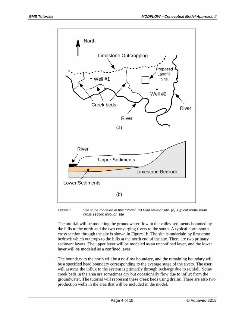
Figure 1 Site to be modeled in this tutorial. (a) Plan view of site. (b) Typical north-south cross section through site

The tutorial will be modeling the groundwater flow in the valley sediments bounded by

the hills to the north and the two converging rivers to the south. A typical north-south

cross section through the site is shown in Figure 1b. The site is underlain by limestone

bedrock which outcrops to the hills at the north end of the site. There are two primary

sediment layers. The upper layer will be modeled as an unconfined layer, and the lower

layer will be modeled as a confined layer.

The boundary to the north will be a no-flow boundary, and the remaining boundary will

be a specified head boundary corresponding to the average stage of the rivers. The user

will assume the influx to the system is primarily through recharge due to rainfall. Some

creek beds in the area are sometimes dry but occasionally flow due to influx from the

groundwater. The tutorial will represent these creek beds using drains. There are also two

production wells in the area that will be included in the model.



NOTE: Although the site modeled in this tutorial is an actual site, the landfill and the

hydrogeologic conditions at the site have been fabricated. The stresses and boundary

conditions used in the simulation were selected to provide a simple yet broad sampling of

the options available for defining a conceptual model.

3 Getting Started

Do the following to get started:

1. If necessary, launch GMS.

2. If GMS is already running, select the File | New command to ensure that the

program settings are restored to their default state.

4 Importing the Project

The first step is to import the East Texas project. This will read in the MODFLOW

model, the solution, and all other files associated with the model.

To import the project, do as follows:

1. Select the Open button.

2. In the Open dialog, locate and open the directory entitled

Tutorials\MODFLOW\modfmap\sample1.

3. Select the file entitled “modfmap.gpr.”

4. Click the Open button.

5 Saving the Project

Before making any changes, save the project under a new name.

1. Select the File | Save As command.

2. Save the project with the name “modfmapII.”

Be sure to hit the Save button periodically as the model is developed.

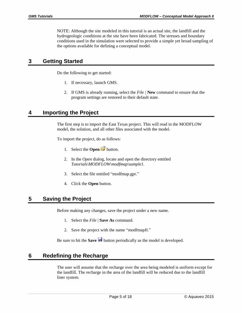
6 Redefining the Recharge

The user will assume that the recharge over the area being modeled is uniform except for

the landfill. The recharge in the area of the landfill will be reduced due to the landfill

liner system.



6.1 Creating the Landfill Boundary

Next, the user will create the arc delineating the boundary of the landfill. In this tutorial,

the user will import the boundary from an existing landfill shapefile.

1. Click on “GIS Layers” folder in the Project Explorer.

2. Select the GIS | Add Shapefile Data menu command.

3. Choose Tutorials\MODFLOW\modfmap\

4. Select the “landfill_arcs.shp” file.

5. Click Open.

Now that the shapefile is imported, the user will convert this shape file into feature

objects in the “Recharge” coverage.

6. Expand the “Map Data” folder.

7. Expand the “East Texas” conceptual model.

8. Make the “Recharge” coverage the active one by selecting it in the Project

Explorer.

9. Select “landfill_arcs.shp” in the “GIS Layers” folder in the Project Explorer.

10. Select the GIS | Shapes Feature Objects command

11. Select the Yes button to map all visible shapes.

12. In the GIS to Feature Objects Wizard dialog, select the Next button.

13. Select Elevation for the ARC_ELEV.

14. Select Next then Finish to complete the process.

The landfill is now created.

6.2 Rebuilding the Polygons

Now that the landfill boundary is defined, it is necessary to rebuild the polygons.

1. Select the Build Polygons macro.

6.3 Assigning the Recharge Values

Now that the recharge zones are redefined, it is possible to assign the recharge values for

the landfill polygon.



1. Click on the “Recharge” coverage.

2. Select the Select Polygons tool.

3. Double-click on the landfill polygon.

4. In the Attribute Table dialog, change the Recharge rate to “0.00006.”

Note: This recharge rate is small relative to the rate assigned to the other polygons. The

landfill will be capped and lined and thus will have a small recharge value. The recharge

essentially represents a small amount of leachate that escapes from the landfill.

5. Select the OK button.

7 Redefining the Hydraulic Conductivity

In the previous tutorial, the user only simulated a one-layer model. In this tutorial, the

user will make a two-layer model. Thus, it is necessary to define the hydraulic

conductivity for the second layer and the vertical anisotropy for both layers. Similar to

the previous tutorial, the user will also use constant values for the second layer.

7.1 Turning on Vertical Anisotropy

1. Right-click on the “Layer 1” coverage.

2. Select the Coverage Setup command from the pop-up menu.

3. In the Coverage Setup dialog, from the Areal Properties list, turn on Vertical

anis.

4. Click OK.

5. Double-click on the landfill polygon in the “Layer 1” coverage.

6. In the Attribute Table dialog, change the Vertical anis. to “4.” This means that

the vertical hydraulic conductivity with be one fourth of the horizontal

conductivity.


7.2 Copying the Layer 1 Coverage

The user will create the “Layer 2” coverage by copying the “Layer 1” coverage.


2. Select the Duplicate command from the pop-up menu.

3. Right-click on the “Copy of Layer 1” coverage.



4. Select the Properties command.

5. In the Properties dialog, change the name of the new coverage to “Layer 2.”

6. Click OK.


8. Select the Coverage Setup command.

9. In the Coverage Setup dialog, change the Default layer range to go from “2” to

“2.”


7.3 Specify the Coverage Attributes

For the new layer, do the following:

1. Select the “Layer 2” coverage in the Project Explorer.

2. Double-click on the landfill polygon

3. In the Attribute Table dialog, change the Horizonal K to “10.”


8 Modifying the Local Source/Sink Coverage

Since our model will have two layers, when mapping the conceptual model to the grid, it

will be necessary to specify which grid layer the wells should be placed in. There are

three ways to do this.

The simplest way is to specify the grid layer in the conceptual model, but that requires

the user to know how many grid layers he or she will have and where they will be when

building the conceptual model. Also, if the user decides to add or subtract grid layers

later, he or she will have to remember to change the conceptual model.

The second way is to use a well screen with the WEL package. This allows the user to

specify the top and bottom of the screened interval of the well. When the conceptual

model is mapped to the grid, the well will be placed automatically in the appropriate grid

layer (or layers) based on which grid layers intersect the well screen. If multiple grid

layers are intersected by the well screen, multiple wells will be created.

The third way is to use the MNW2 package and define the screened interval. The MNW2

package is a more realistic well package that better models partially penetrating wells and

wells that have more than one screened interval and/or draw from multiple grid layers.

This tutorial will use this option.



The user will also modify the conceptual model so that it uses real terrain data for

elevations. The terrain elevations will come from a raster. Also, the user will use the

raster to define the drain elevations. When the drain arcs are discretized onto the model

grid, the cells that intersect the arcs will be found. Then the drain elevation is interpolated

from the raster to the cell centers.

This method is particularly helpful with large models where otherwise the user would

have to manually determine and enter the elevation for each drain at the arc nodes.

8.1 Turn on MNW2

It is necessary to make the MNW2 properties available in the coverage.

1. Right-click the “Sources & Sinks” coverage in the Project Explorer.

2. Select the Coverage Setup command from the pop-up menu.

3. In the Coverage Setup dialog, in the list of Sources/Sinks/BCs, turn on Wells

(MNW2).

4. Click OK to exit.

8.2 Modifying the existing well

First edit the eastern well.

1. Select the “Sources & Sinks” coverage in the Project Explorer.

2. Switch to the Select Points\Nodes tool.

3. Select the well on the eastern (right) side of the model.

4. Select Properties button.

5. In the Attribute Table dialog, change the Type to “well (MNW2).”

6. Scroll to the right and enter “-300.0” in the Qdes field.

7. Make sure the Vertical Boreline option is on.

8. For the LOSSTYPE field, choose the “THIEM” option.

9. Click on the … button under Boreline.

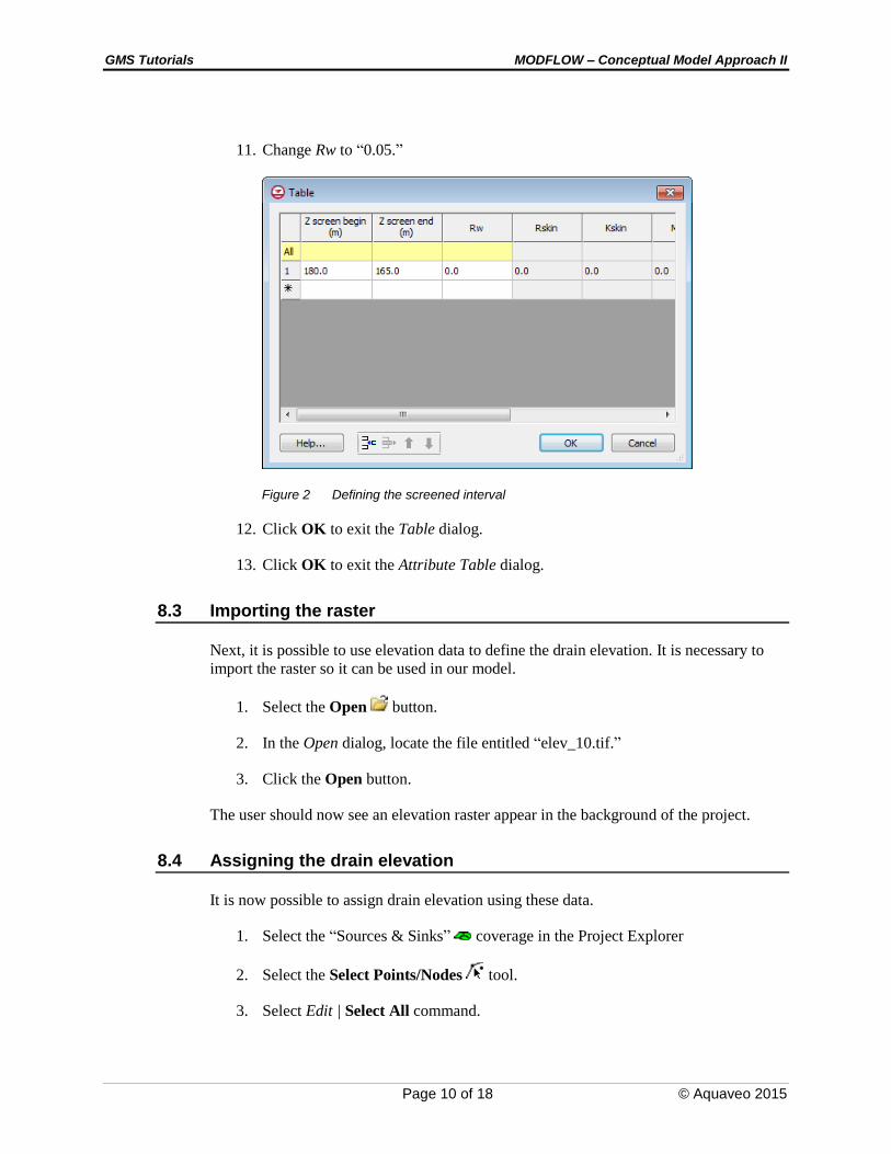
10. In the Table dialog, enter “180” (m) for Z screen begin and “165” (m) for Z

screen end.

These values make the well screen go through both layer 1 and layer 2.



11. Change Rw to “0.05.”

Figure 2 Defining the screened interval

12. Click OK to exit the Table dialog.

13. Click OK to exit the Attribute Table dialog.

8.3 Importing the raster

Next, it is possible to use elevation data to define the drain elevation. It is necessary to

import the raster so it can be used in our model.

1. Select the Open button.

2. In the Open dialog, locate the file entitled “elev_10.tif.”

3. Click the Open button.

The user should now see an elevation raster appear in the background of the project.

8.4 Assigning the drain elevation

It is now possible to assign drain elevation using these data.

1. Select the “Sources & Sinks” coverage in the Project Explorer

2. Select the Select Points/Nodes tool.

3. Select Edit | Select All command.



4. Select Properties button.

5. In the Attribute Table dialog, change the BC type to “drain.”

6. In the first row under Bot. elev., click on the drop-down box and select

“<Raster>.”

7. In the Select Raster window, select the “elev_10.tif.”


9. Select the OK button exit the Attribute Table dialog.

9 Recreating the Grid

It is now possible to create a new two layer grid.

1. Select the Feature Objects | Map 3D Grid command.

2. Click OK twice to confirm deletion of the grid and the current MODFLOW

model.

Notice that the grid is dimensioned using the data from the Grid Frame. If a Grid Frame

does not exist, the grid is defaulted to surround the model with approximately 5% overlap

on the sides. Also note that the number of cells in the x and y dimensions cannot be

altered. This is because the number of rows and columns and the locations of the cell

boundaries will be controlled by the refine point data entered at the wells.

3. In the Create Finite Difference Grid dialog, in the Z-Dimension field, change

Number cells to “2.”


10 Initializing the MODFLOW Data

Now that the grid is constructed and the active/inactive zones are delineated, the next step

is to convert the conceptual model to a grid-based numerical model. Before doing this,

however, the user must first initialize the MODFLOW data:

1. Right-click on the “grid” item in the Project Explorer.

2. Select the New MODFLOW command.

3. When the MODFLOW Global/Basic Package dialog appears, select the OK

button.



11 Defining the Active/Inactive Zones

Now that the grid is created, the next step is to define the active and inactive zones of the

model. This is accomplished automatically using the information in the local

sources/sinks coverage.

1. Select the “Map Data” folder in the Project Explorer.

2. Select the “Sources&Sinks” coverage to make it active.

3. Select the Select Polygons tool.

4. Select one of the polygons.

5. Select the Properties button.

6. In the Attribute Table dialog, confirm that the layer assignment for the From

layer is “1” and the To layer is “2.”

7. Click OK.

8. Select the Feature Objects | Activate Cells in Coverage(s) command.

Each of the cells in the interior of any polygon in the local sources/sinks coverage is

designated as active and each cell which is outside of all of the polygons is designated as

inactive. Notice that the cells on the boundary are activated such that the no-flow

boundary at the top of the model approximately coincides with the outer cell edges of the

cells on the perimeter while the specified head boundaries approximately coincide with

the cell centers of the perimeter cells.

12 Interpolating Layer Elevations

Now it is necessary to define the layer elevations and the starting head. Since this tutorial

is using the LPF package, top and bottom elevations are defined for each layer regardless

of the layer type. For a two layer model, it is necessary to define a layer elevation array

for the top of layer 1 (the ground surface), the bottom of layer 1, and the bottom of layer

2. It is assumed that the top of layer 2 is equal to the bottom of layer 1.

One way to define layer elevations is to import a set of scatter points defining the

elevations and interpolate the elevations directly to the layer arrays. This can be done

with scatter points as well as rasters. In this case, the user will use a raster for the top of

the gird and scatter points for the elevations of the bottom of layer 1 and the bottom of

layer 2.

Layer interpolation is covered in depth in the “MODFLOW – Interpolating Layer Data”

tutorial.



12.1 Delete the Layer Elevations Coverage

The model that the user started with included a coverage that defined a constant top and

bottom elevation for the entire model area. It is no longer desirable to use that method for

defining layer elevations. Instead, the user will interpolate layers from scatter points to

create a more realistic, varying terrain. It is therefore necessary to delete the Layer

Elevations coverage.

1. Right-click on the the “Layer Elevations” coverage.

2. Select the Delete command.

12.2 Interpolating the Heads and Elevations

Next, the user will interpolate the ground surface elevations and starting heads to the

MODFLOW grid.

1. Right-click on the “elev_10.tif” raster.

2. Select the Interpolate To | MODFLOW Layers menu command.

This is the dialog that allows the user to tell GMS which datasets to interpolate to which

MODFLOW arrays. The dialog is explained fully in the “MODFLOW – Interpolating

Layer Data” tutorial.

3. In the Interpolate to MODFLOW Layers dialog, highlight the “elev_10.tif” raster

and the “Starting Heads 1” array, and click the Map button.

4. Highlight the “elev_10.tif” raster and the “Starting Heads 2” array, and click the

Map button.

5. Highlight the “elev_10.tif” raster and the “Top Elevations Layer 1” array, and

click the Map button.

6. Select the OK button to perform the interpolation.

12.3 Interpolating the Layer Elevations

Do as follows to interpolate the layer elevations for the bottom of layers 1 and 2:

1. In the Project Explorer, expand the “2D Scatter Data” folder.

2. Right-click on the “elevs” scatter set.

3. Select the Interpolate To | MODFLOW Layers command.

GMS automatically mapped the Bottom Elevations Layer 1 and Bottom Elevations Layer

2 arrays to the appropriate data sets based on the data set name.



4. Select the OK button to exit the Interpolate to MODFLOW Layers dialog.

12.4 Adjusting the Display

Now that the interpolation is finished, the user can hide the scatter point sets and the grid

frame.

1. Turn off the “grid frame” .

2. Turn off the “GIS Layers” folder.

12.5 Viewing the Model Cross Sections

To check the interpolation, the user will view a cross section.

1. Select the “3D Grid Data” folder in the Project Explorer.

2. Using the Select Cell tool, select a cell somewhere near the center of the

model.

3. Select the Side View button.

The user may wish to use the arrow buttons in the Tool Palette to view different columns

in the grid.

Note that on the right side of the cross section, the bottom layer pinches out and the

bottom elevations are greater than the top elevations. This must be fixed before running

the model.

12.6 Fixing the Elevation Arrays

GMS provides a convenient set of tools for fixing layer array problems. These tools are

located in the Model Checker and are explained fully in the “MODFLOW – Interpolating

Layer Data” tutorial.

1. Select the MODFLOW | Check Simulation command.

2. Select the Run Check button.

3. Select the Fix Layer Errors button at the right of the dialog.

Notice that many errors were found for layer 2. There are several ways to fix these errors.

This tutorial will use the Truncate to bedrock option. This option makes all cells below

the bottom layer inactive.

4. In the Fix Layer Errors dialog, select the Truncate to bedrock option.

5. Select the Fix Affected Layers button.



6. Select the OK button to exit the Fix Layer Errors dialog.

7. Select the Done button to exit the Model Checker dialog.

Notice that the layer errors have been fixed. Another way to view the layer corrections is

in plan view.

8. Select the Plan View button.

9. In the Ortho Grid Toolbar, select the up

arrow to view the second layer.

Notice that the cells at the upper (northern) edge of the model in layer 2 are inactive.

10. Switch back to the top layer by selecting the down arrow .

13 Converting the Conceptual Model

It is now possible to convert the conceptual model from the feature object-based

definition to a grid-based MODFLOW numerical model.

1. Right-click on the “East Texas” conceptual model.

2. Select the Map To | MODFLOW / MODPATH command.

3. In the Map Model dialog, make sure the All applicable coverages option is

selected.

4. Select OK.

Notice that the cells underlying the drains, wells, and specified head boundaries were all

identified and assigned the appropriate sources/sinks. The heads and elevations of the

cells were determined by linearly interpolating along the specified head and drain arcs.

The conductances of the drain cells were determined by computing the length of the drain

arc overlapped by each cell and multiplying that length by the conductance value

assigned to the arc. In addition, the recharge and hydraulic conductivity values were

assigned to the appropriate cells.

14 Checking the Simulation

At this point, the MODFLOW data has been completely defined, and it is possible to run

the simulation. First run the Model Checker to see if GMS can identify any mistakes that

may have been made.


2. Select the MODFLOW | Check Simulation command.



3. Select the Run Check button. There should be no errors.

4. Select the Done button to exit the Model Checker dialog.

15 Saving the Project

Now the user is ready to save the project and run MODFLOW.

1. Select the Save button.

Note: Saving the project not only saves the MODFLOW files but it saves all data

associated with the project including the feature objects and scatter points.

16 Running MODFLOW

It is now possible to run MODFLOW.

1. Select the MODFLOW | Run MODFLOW command. At this point,

MODFLOW is launched and the Model Wrapper appears.

2. When the solution is finished, select the Close button.

A set of contours should appear. To view the contours for the second layer, do as follows:

3. Select the up arrow in the Ortho Grid Toolbar.

4. After viewing the contours, return to the top layer by selecting the down arrow

.

17 Viewing the Water Table in Side View

Another interesting way to view a solution is in side view.

1. Select the Select Cell tool.

2. Select a cell somewhere near the well on the right side of the model.

3. Select the Side View button.

Notice that the computed head values are used to plot a water table profile. Use the arrow

buttons in the Mini-grid Toolbar to move back and forth through the grid. The user

should see a cone of depression at the well. When finished, do as follows:

4. Select the Plan View button.



18 Viewing the Flow Budget

The MODFLOW solution consists of both a head file and a cell-by-cell flow (CCF) file.

GMS can use the CCF file to display flow budget values. For example, the user may want

to know if any water exited from the drains. This can be accomplished simply by clicking

on a drain arc.

1. Select the “Map Data” folder in the Project Explorer.

2. Choose the Select Arcs tool.

3. Click on the rightmost drain arc.

Notice that the total flow through the arc is displayed in the strip at the bottom of the

window. Next, the user will view the flow to the river.

4. Click on one of the specified head arcs at the bottom and view the flow.

5. Hold down the Shift key and select each of the specified head arcs.

Notice that the total flow is shown for all selected arcs. Flow for a set of selected cells

can be displayed as follows:


7. Select a group of cells by dragging a box around the cells.

8. Select the MODFLOW | Flow Budget command.

The Flow Budget dialog shows a comprehensive flow budget for the selected cells.

9. Select OK to exit the dialog.

10. Click anywhere outside the model to unselect the cells.

19 Conclusion

This concludes the “MODFLOW – Conceptual Model Approach II” tutorial. Here are the

main points from this tutorial:

It is possible to import shapefiles and convert them to feature objects for use in

the conceptual model.

Well screens can be used to automatically locate the correct a 3D grid layer in

which the wells are located.

The MNW2 package more accurately models wells that are screened across

multiple layers.



Elevations for boundary conditions, such as drains, can be specified using a

raster.

It is possible to specify things like layer elevations and hydraulic conductivities

using polygons in the conceptual model, but that will result in stair-step-like

changes. For smoother transitions, it is possible to use 2D scatter points and

interpolation.

v. 10 - aquaveogmstutorials-10.0.aquaveo.com/modflow-conceptual... · build a multi-layer modflow...

Documents