v mine graphs

V Mine Graphs

Vipul SinghDept. of Computer Science

[email protected]

Venkata Krishna PillutlaDept. of Computer Science

[email protected]

December 2, 2014

AbstractIn this project, we implement various graph algorithms for computing the degree

distributions, pagerank, connected components, radii of the vertices, eigen-decompositionof the adjacency matrix, and triangle counts using SQL. We also perform anomaly de-tection by extracting features from the egonets. Finally, we apply these operations on20 real world datasets in an attempt to identify recurring and anomalous patterns inthese graphs. In addition, we extend the package GraphMiner to perform the k-coresdecomposition of graphs too.

1 Introduction

Graphs provide a convenient abstraction to model and view data, systems and application([11]). Common graphs include the internet, social networking, to name a few. Analyzingthese graphs is of great interest for observing trends and patterns. Outliers are also ofgreat interest- for instance, in anomaly detection helps detect intruders in security networks,spammers and agents with malicious intent on the internet ([14], [2]).

With data becoming more freely available and in greater volume, and with increasingcomputing power, emergence of distributed computing platforms such as Hadoop and agrowing demand for information hidden in the data, lots of systems and algorithms, takingpopular Graph Mining to Hadoop have emerged. Worth noting are Pegasus ([7]), Hadi ([8]),Eigenvalues ([10], [12]) to name a few.

For moderate sized applications, using SQL wrapped in a host programming language([4]) is more pragmatic. The advantages of such a system are two-fold: firstly, the speed-upachieved on Hadoop is outweighed by the overheads of running several tasks on Hadoop;secondly, it is much easier for people to use SQL.

The package GraphMiner was made with this motivation ([4]). The package implementsvarious graph algorithms for computing the degree distributions, pagerank, connected com-ponents, radii of the vertices, eigendecomposition of the adjacency matrix, belief propagationand triangle counts. Our contributions to this project are the following:

1

• Implement the k-cores algorithm in the existing framework ([3]).• Test various features with Unit Tests.• Run results with two large datasets.

2 Survey

Next we list the papers that each member read, along with their summary and critique.

2.1 Papers read by Venkata Krishna Pillutla

2.1.1 Pegasus: Peta-Scale Graph Mining System- Implementation and Obser-vations [7]

Main Idea: The authors describe an open source library called PEGASUS to mine graphsof sizes reaching several petabytes efficiently over Hadoop in a distributed manner. Theentire library is based on a single primitive, which the authors name GIM-V for GeneralizedIterated Matrix-Vector multiplication. As the name suggests, it is a generalized version of amatrix vector multiplication that replaces the multiplication, summing and assignment op-erations of v = Au with arbitrary functions. Further, this operation can be implemented inSQL, thus describing This primitive can be made to achieve several functionalities by usingappropriate user-defined functions. The paper goes on the describe how PageRank, RandomWalks with Restarts and Diameter Estimation in large graphs can can be implemented usingGIM-V, thus establishing the potency of this operation. Further, the authors propose a newalgorithm HCC for finding connected components of a graph.The authors then go on to describe a fast method to implement GIM-V as Map and Reducefunctions on Hadoop. Since this primitive is used repeatedly, it is of utmost importancethat it is as fast as possible. Towards this end, the authors suggest several optimizationsto the base GIM-V algorthim: using Block Multiplication, Clustered Edges or both for bestperformance. Also, variants using Diagonal Block Iterations and Node Renumbering wereproposed for the HCC algorithm. The optimizations reduce the running time by about fivetimes. The authors demonstrate, with experiments, that the system scales linearly with thenumber of edges in the graph and number of machines in the network. The system was alsotested on real-world web-scale graphs of Wikpedia, LinkedIn, Yahoo among others. In theaforementioned applications, other interesting observations such as power laws relations ofcounts of versus size of connected components, page rank distributions, to name a few, weremade. Further, these plots were used to detect outliers and anomalies.Shortcomings: The proposed system does not include a distributed Eigensolver. Eigenvaluesand eigenvectors contain a lot of information and could be used for applications such asspectral clustering. The matrices associated with Peta-scale graphs will be huge and a dis-tributed eigensolver seems necessary. Further, implemented these algorithms and operationson existing parallel/distributed relational database systems would make sophisticated graphmining tools accessible to more people and in an easier manner.

2

2.1.2 Spectral Analysis for Billion-Scale Graphs: Discoveries and Implementa-tion ([6])

Eigenvalues and eigenvectors of a graphs adjacency matrix make answers questions aboutpatterns and anomalies in the graph very cheap. Existence of triangles or cliques (or near-cliques) always point to something interesting in the graph. The authors propose to solvesuch problems on large scale in Hadoop with a design and implantation that is scalable.The paper discusses traditional approaches to solving eigenvalue problems: Power Iterations,QR Method, Lanczos iterations. The only method to find the top k eigenvalues and eigenvec-tors that was considered tractable with respect to the scale of the problem and the setting(Hadoop) was the Lanczos-SO algorithm that only selectively renormalized basis vectors.The most expensive operation of this algorithm is matrix-vector multiplication and this canbe parallelized in Hadoop.To make the system scalable to graphs with sizes in billions, operations were selectively par-allelized. Operations like the aforementioned matrix-vector multiplications are intractableserially given the scale of the problem and have to be performed in parallel. There are,however, operations such as computing a matrix spectral norm are faster serially becauserunning a job on Hadoop has some synchronization overheads. Other optimizations involvedwere using blocks instead of single elements and exploiting skewness in matrix-vector andmatrix-matrix products.The authors further show with experimental proof that the running time of their methodscaled linearly with the number of edges and machines. Experiments also show that the op-timizations proposed significantly reduce running time. To conclude, they have, with carefuldesign decisions, an effective and scalable eigensolver.Shortcomings and future research direction: Each Map-Reduce task incurs significant over-head: some amount of book- keeping and synchronization is required before the actualcomputation can start. Since each iteration of the proposed method launches several Map-Reduce tasks, the fraction of fraction of the running time actually spent on computation islikely to be small. A future direction would be to reduce these overheads and maybe run theentire algorithm as a single task, but with appropriate parallelism. Further, if this methodcould be made asynchronous, it would greatly reduce the synchronization overheads andincrease the utilization of the CPUs.

2.1.3 Unifying Guilt-by-Association Approaches: Theorems and Fast Algo-rithms ([9])

Guilt-by-Association or Label propagation is a problem where neighbors are assumed to in-fluence label, either positively or negatively: homophily and heterophily respectively. Thepaper reviews three basic algorithms that achieve this goal: Random Walk with Restarts(RWR), Semi-supervised Learning (SSL) and Belief Propagation (BP), and proposes a new,faster, scalable algorithm called Fast Belief Propagation (FaBP) over Hadoop.RWR is the method underlying page rank but doesnt support heterophily. Neither does SSL

3

but both methods are guaranteed to converge. BP proposes heterophily but convergenceis not guaranteed and depends on choice of parameters. FaBP combines the best of bothworlds and provides both convergence guarantees and support for heterophily.The authors unify all algorithms in that they solve a linear system of the form Ax = b wherewe solve for x, given the prior beliefs b and the data and parameter dependent matrix A.Also, inverting a matrix is costly operation and is intractable in scales under considerationhere, so the authors propose to use the Power Method. The authors analyze in great detailthe theoretical conditions when the proposed FaBP algorithm converges and use these resultsto design the algorithm.The authors show experimentally that FaBP and BP agree when run with the same pa-rameters but FaBP guarantees convergence. It was also observed the accuracy is not verysensitive to the parameters as long as the parameters are in acceptable ranges. Further, theauthors observe that FaBP scales linearly with the number of edges in the graph and thenumber of machines and runs twice as fast as BP. Further, this method can be extendednaturally for multiple labels.Short-comings: The graphs are considered to be static. The work does not consider time-evolving graphs and how labels change with time. Also, the solution of the system dependsgreatly on prior beliefs. To get a good output, the priors should be realistically modeled.But then again, this is a necessity in Bayesian statistics.

2.2 Papers read by Vipul Singh

2.2.1 k-core decomposition: a tool for the visualization of large scale networks([3])

The authors propose a visualization algorithm to display several topological and hierarchicalproperties of large scale networks. This is of interest these days because we are dealing withgraphs that have millions of nodes, representing web traffic, connections on social networks,etc. It becomes important then to focus on particular subsets of the graph, namely k-cores,which are sets of vertices, each having degree ≥ k within the set. Larger values of k for acore are in correspondence with a more central position in the network.

Recursive removal of vertices having degree less than a given k can break the originalnetwork into various connected components, each of which might even be once again brokenby the subsequent decomposition. The visualizer represents each vertex i in polar coordi-nates (ρi, αi): the radius is a function of the coreness of the vertex i and its neighbors; theangle varies with cluster number. Eventually, k-shells get displayed as concentric shells, theinnermost one being the set of vertices with highest coreness. Colour of shells is assignedaccording to vibgyor scale, while the size of a vertex is proportional to the logarithm ofits degree, thus retaining and showing some properties from the original graph. Differentcomponent cores get represented with different centres and their sizes vary with the numberof nodes in each.

4

Since this visualisation shows the network in layers, it gives a direct way to distinguishthe different hierarchies and structural organization by using the radial width of the shells,the presence and size of clusters of vertices in the shells, the correlations between degreeand coreness, the distribution of the edges interconnecting vertices of different shells, etc.The authors further go on to provide examples where the algorithm allows identification ofcharacteristic fingerprints and hierarchies in real networks, e.g.: identification of the differenthierarchical arrangement of the Internet network when visualized at the Autonomous systemlevel and the Router level.

A shortcoming would be that such visualisation becomes highly dense with increasingnumber of nodes and hence, it becomes tough to observe properties of individual nodes orsmall clusters at such scales. The k-core decomposition algorithm in itself is O(n+ e) wheren and e are the number of vertices and edges, respectively. Hence, for even moderately densegraphs with a million nodes, this is a time-taking process in itself. A faster algorithm, evenif probabilistic or approximate, would be very useful in such a setting.

2.2.2 Mining Large Graphs: Algorithms, Inference, and Discoveries ([5])

Belief Propagation (BP) has a running time that scales linearly with the number of edges inthe graph, which becomes significant when we have a billion edges. The authors handle thescenario where the graphs would not fit in main memory. BP works by iteratively running 2equations. In a large scale algorithm for MapReduce though, random access is not allowedand we look for a recursive solution, which is made tricky by the message that exists in oneof the denominators. To overcome this, the Line Graph Fixed Point (LFP) method has beenformulated.

Given a directed graph G, its directed line graph L(G) is a graph such that each node ofL(G) represents an edge of G, and there is an edge from vi to vj of L(G) if the correspondingedges ei and ej form a length-two directed path from ei to ej in G.([5]). The exact recursiveformulation is derived on this line graph, which is seen to boil down to some vector-matrixmanipulations. The run-time of this algorithm is O(n+e

M) where M is the number of machines

available for parallel execution. From experiments, it is concluded that HA-LFP is the onlysolution when the nodes information can not fit in memory. It even enjoys the fault toleranceprovided by HADOOP.

Future work could involve using properties of line graphs to speed up the matrix-vectoroperations, because these can be time-consuming and a potential overhead if the matricesbecome huge and dense. Also, we can have other metrics than convergence of message vectorfor stopping the algorithm.

5

2.2.3 RTG: A Recursive Realistic Graph Generator using Random Typing ([1])

In order to simulate real-world graphs and to have more samples for purpose of study onpatterns and characteristics, we need to build realistic graph generators. This paper de-scribes one such generator that relies on the idea of random typing, similar to the proposedby Miller in his experiment where a monkey is supposed to hit random keys and generatewords in the long run.

Firstly, a simple to implement algorithm is presented which suffers from some drawbacksin terms of it matching real-world graphs due to lack of homophily and community structure.Each unique word typed by the monkey is supposed to represent a node in the output graph.The word sequence is marked as source and destination, alternatingly. Divide the sequenceof words into groups of two and link the first node to the second node in each pair. If twonodes are already linked, the weight of the edge is simply increased by 1. Therefore, if Wwords are typed, the total weight of the output graph is W/2. Smoothing of the degree distri-bution to achieve a power law is obtained now by assigning unuequal probabilities to the keys.

Finally, the authors propose a two-dimensional keyboard that generates source and desti-nation labels in one shot. After a key is selected, its row character is appended to the sourcelabel, and the column character to the destination label. This process repeats recursively.Introduction of an imbalance factor brings about the properties that were missing earlier.

Future work could involve developing graphs after learning some features from a set ofknown real-world graphs. For example, some social networks may have representative graphsthat differ from the general set and hence, we may not want to have the same set of gener-ators for all types.

3 Proposed and Implemented Methods

3.1 k-cores

We implement the algorithm described in ([3]).Input: Edge table, listing out all the pairs of nodes connected together in the undirectedgraph.Output: List of k-cores, in the format - vertex followed by k-core idAlgorithm: Initial count is the total number of edges in the input table.

1. Calculate degree of each vertex from the edge-table.

2. Count the number of edges in the table. If same as in previous iteration, then go tostep 5.

3. For each vertex with degree less than k, delete all edges containing that vertex.

6

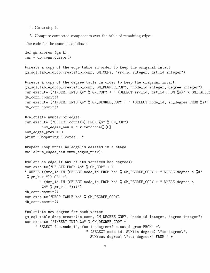
4. Go to step 1.

5. Compute connected components over the table of remaining edges.

The code for the same is as follows:

def gm_kcores (gm_k):

cur = db_conn.cursor()

#create a copy of the edge table in order to keep the original intact

gm_sql_table_drop_create(db_conn, GM_COPY, "src_id integer, dst_id integer")

#create a copy of the degree table in order to keep the original intact

gm_sql_table_drop_create(db_conn, GM_DEGREE_COPY, "node_id integer, degree integer")

cur.execute ("INSERT INTO %s" % GM_COPY + " (SELECT src_id, dst_id FROM %s)" % GM_TABLE)

db_conn.commit()

cur.execute ("INSERT INTO %s" % GM_DEGREE_COPY + " (SELECT node_id, in_degree FROM %s)" % GM_NODE_DEGREES)

db_conn.commit()

#calculate number of edges

cur.execute ("SELECT count(*) FROM %s" % GM_COPY)

num_edges_new = cur.fetchone()[0]

num_edges_prev = 0

print "Computing K-cores..."

#repeat loop until no edge is deleted in a stage

while(num_edges_new!=num_edges_prev):

#delete an edge if any of its vertices has degree<k

cur.execute("DELETE FROM %s" % GM_COPY + \

" WHERE ((src_id IN (SELECT node_id FROM %s" % GM_DEGREE_COPY + " WHERE degree < %d"

% gm_k + ")) OR" +\

" (dst_id IN (SELECT node_id FROM %s" % GM_DEGREE_COPY + " WHERE degree <

%d" % gm_k + ")))")

db_conn.commit()

cur.execute("DROP TABLE %s" % GM_DEGREE_COPY)

db_conn.commit()

#calculate new degree for each vertex

gm_sql_table_drop_create(db_conn, GM_DEGREE_COPY, "node_id integer, degree integer")

cur.execute ("INSERT INTO %s" % GM_DEGREE_COPY +

" SELECT foo.node_id, foo.in_degree+foo.out_degree FROM" +\

" (SELECT node_id, SUM(in_degree) \"in_degree\",

SUM(out_degree) \"out_degree\" FROM " +

7

" (SELECT dst_id \"node_id\", count(*) \"in_degree\", \

0 \"out_degree\" FROM %s" % GM_COPY +

" GROUP BY dst_id" +

" UNION ALL" +

" SELECT src_id \"node_id\", 0 \"in_degree\", \

count(*) \"out_degree\" FROM %s" % GM_COPY +

" GROUP BY src_id) \"TAB\" " +

" GROUP BY node_id) AS foo")

db_conn.commit()

num_edges_prev = num_edges_new

cur.execute ("SELECT count(*) FROM %s" % GM_COPY)

num_edges_new = cur.fetchone()[0]

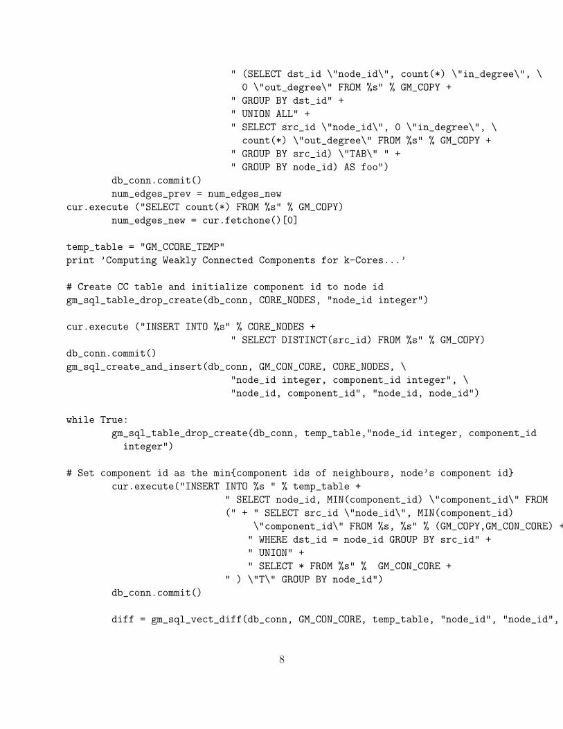
temp_table = "GM_CCORE_TEMP"

print ’Computing Weakly Connected Components for k-Cores...’

# Create CC table and initialize component id to node id

gm_sql_table_drop_create(db_conn, CORE_NODES, "node_id integer")

cur.execute ("INSERT INTO %s" % CORE_NODES +

" SELECT DISTINCT(src_id) FROM %s" % GM_COPY)

db_conn.commit()

gm_sql_create_and_insert(db_conn, GM_CON_CORE, CORE_NODES, \

"node_id integer, component_id integer", \

"node_id, component_id", "node_id, node_id")

while True:

gm_sql_table_drop_create(db_conn, temp_table,"node_id integer, component_id

integer")

# Set component id as the min{component ids of neighbours, node’s component id}

cur.execute("INSERT INTO %s " % temp_table +

" SELECT node_id, MIN(component_id) \"component_id\" FROM

(" + " SELECT src_id \"node_id\", MIN(component_id)

\"component_id\" FROM %s, %s" % (GM_COPY,GM_CON_CORE) +

" WHERE dst_id = node_id GROUP BY src_id" +

" UNION" +

" SELECT * FROM %s" % GM_CON_CORE +

" ) \"T\" GROUP BY node_id")

db_conn.commit()

diff = gm_sql_vect_diff(db_conn, GM_CON_CORE, temp_table, "node_id", "node_id",

8

"component_id", "component_id")

# Copy the new component ids to the component id table

gm_sql_create_and_insert(db_conn, GM_CON_CORE, temp_table, \

"node_id integer, component_id integer", \

"node_id, component_id", "node_id, component_id")

print "Error = " + str(diff)

# Check whether the component ids has converged

if (diff == None or diff == 0):

print "Component IDs for k-cores have converged"

break

cur.execute ("SELECT count(distinct component_id) FROM %s" % GM_CON_CORE)

num_components = cur.fetchone()[0]

print "Number of k_cores formed = ", num_components

# Drop temp tables

gm_sql_table_drop(db_conn, temp_table)

num_edges_new = num_edges_new/2

gm_sql_table_drop_create(db_conn, CORE_EDGES, "src_id integer, dst_id integer")

cur.execute ("INSERT INTO %s" % CORE_EDGES + " (SELECT * FROM %s" % GM_COPY +

" LIMIT %d" %num_edges_new + " )")

db_conn.commit()

cur.close()

3.2 Unit Tests

The Unit Tests have been designed to be small enough and yet evoke many different casesand boundary conditions in the algorithms. The output is hard-coded and compared. De-scriptions of the units tests have been provided along with the graphs. Of special interestis Unit Test 5, which has a 5-core of 8 vertices, each with degree 5 or 6, and some othervertices of smaller degrees. This is to check that the k-cores works for graphs that are notcliques as well.

4 Experiments

4.1 Phase 1

We run our algorithms on wiki-Vote and soc-Epinions1 datasets. Following is a summary ofour results:

9

Figure 1: Unit Test 1 has two connected directed paths, one of the simplest graphs.

Figure 2: Unit Test 2 is a directed clique with one connected component. This thoroughlyverifies degree distributions.

Figure 3: Unit Test 3 is an undirected 5-clique. This should have an empty 5-core and is asanity check.

4.1.1 wiki-Vote

1. We have 24 connected components, 3 of size 3 each, 20 of size 2 each and one with7066 vertices.

2. There is just one 5-core, with 3513 vertices.

10

Figure 4: Unit Test 4 has two undirected 6-clique contributing to two 5-cores. This shouldhave two 5-cores. The small paths connected to the cliques are to check whether unecessaryvertices are pruned away.

Figure 5: Unit Test 5 has two connected components. One of them contains a 5-core,although there is no 5-clique.

4.1.2 soc-Epinions1

1. We have two connected components, one with 75877 vertices and the other with 2.

2. There is just one 5-core, with 19241 vertices.

11

(a) Degree distribution plot for the soc-Epinionsdataset

(b) Degree distribution plot for the wiki-Votedataset

(c) Pagerank scores for nodes in socEpinionsgraph

(d) Pagerank scores for nodes in wiki-Vote graph

Figure 6: Outputs for wiki-Vote and soc-Epinions1

12

4.2 Phases 2 and 3

4.2.1 Indices

We try out various possible indices on tables used in the algorithms namely:

1. For tables that represent edges or matrices, i.e., have two columns that carry some sortof ids, we try out the following 6 cases:

• 0 = no index

• 1 = hash index on first id

• 2 = hash index on second id

• 3 = btree index on first id

• 4 = btree index on second id

• 5 = btree index on pair of ids

2. For tables with single id columns, i.e., ones representing a vector of values, for example,in the eigen-algorithms, we consider:

• 0 = no index

• 1 = hash index on id

• 2 = btree index on id

Algorithm-wise, the tables under consideration are as follows:

Algorithm/Task Tables with 2 ids Tables with 1 iddegree distribution GM TABLE -

pagerank GM TABLE, norm table -radius GM TABLE UNDIRECT -k-cores GM TABLE, GM COPY -

connected components GM TABLE UNDIRECT GM CON COMPeigen eigvec table next basis vect, basis vect 0

basis vect 1, temp vect, temp vect2

We first constructed indexing options on the tables involved in degree distribution, pager-ank, radius and k-cores algorithms. To maintain feasibility, in a single experiment, we use thesame indexing type (0-5) on all tables involved and obtain running time for each. Followingis a summary of which type works best for every dataset-algorithm pair. Note that in somecases, the experiment with no index gave best results, in which case we have mentioned thesecond best index in brackets.

13

Dataset Degree Distribution PageRank Radius k-Coresas-skitter 0(2) 3 2 2

ca-AstroPh 2 5 4 4cit-HepPh 5 3 2 0(3)cit-HepTh 0(3) 4 4 3

com-amazon 5 5 4 5com-dblp 3 3 2 5

email-Enron 1 5 4 4email-EuAll 1 3 1 5

p2p-Gnutella31 4 1 4 3soc-Slashdot 2 3 4 4soc-Epinions 3 0(4) 4 4

wiki-Vote 5 3 3 3

Obervations:

1. The time taken for these 4 algorithms is of the order of 10−1, 101, 102 and 102 secondsrespectively.

2. For computing degree distribution, no single index seems to consistently outperformthe others. Also, the time taken is a fraction of a second in all cases. So, we can chooseno or any index.

3. For page rank algorithm, index#3, i.e., btree index on the src id column, works best.This is because during construction of the norm table, we use a self-join on GM TABLEwherein the condition is equality on src id attribute.

4. While computing radii, we use a join on GM TABLE UNDIRECT with prev hop table,where the dst id attribute from the former is used. Hence, a btree index on the dst idcolumn, i.e., index#4, works best on most datasets.

5. During k-cores computation, in the iterative loop, I select counts of edges, grouped bysrc id as well as by dst id. Index#4 again turns out to be the best here, because btreeindex supports range queries better and is locality-sensitive, which helps in groupingoperations.

A few representative plots can be seen in figure 7. The actual outputs can be found inthe folder graphminer/index analysis/dprk results/.

4.2.2 Indices for connected components and eigen-algorithms

We then experiment on indexing options for these algorithms. Here, we have tables such asGM TABLE, GM TABLE UNDIRECT and eigvec table which have two columns that canbe indexed on. On the othe hand, we also have id-vs-value tables such as GM CON COMPand the vector-tables where we wish to test indices on a single column. So, we tested the6*3=18 possible scenarios, obtained the outputs and have summarized our results below:

14

(a) email-Enron (b) soc-Slashdot

Figure 7: Comparison for runnning-times under various indexing options for two of the tendatasets, for the algorithms concerning degree, pagerank, radius and k-cores

1. For the eigen-algorithms, due to the high number of iterations, it becomes infeasible(time-consuming) to create an index on the vector tables each time, and hence we aremostly better off with indices on just the big 2-column tables.

2. For the eigvec table, btree indices on either column or pair of columns work best. Afew representative plots can be seen in figure 8. The actual outputs can be found inthe folder graphminer/index analysis/eigen results/.

3. For computing connected components, indexing pairs (4, 0), (2, 1) and (4, 1) work wellover almost all datasets. This can be explained using the fact that there is a self-joinon GM TABLE UNDIRECT where equality on its two columns is used, thus indicat-ing that an index on the dst id would be beneficial (indexes #2 and #4). For theGM CON COMP table, there is a full table scan and a group by node id involved. Forthe former, having no index (#0) seems like a good option. A few representative plotscan be seen in figure 9. The actual outputs can be found in the folder graphminer/in-dex analysis/conncomp results/.

4.2.3 Datasets

After finding the best indices for each algorithm, we run them for 20 big datasets andplot/analyse the results. The datasets are listed in Table 1. In the following subsections, weprovide a brief summary of our observations.

4.2.4 5-cores

Figure 10 contains a logscale plot for the number of 5-cores in different datasets.

15

(a) email-Enron (b) as-skitter

Figure 8: Comparison for runnning-times under various indexing options for two of the tendatasets, for the eigen-algorithms

(a) wiki (b) astroph

Figure 9: Comparison for runnning-times under various indexing options for two of the tendatasets, for the connected components algorithm

16

Dataset Category Directed Descriptionas-Caida Autonomous system N ISP Ranking from topological dataas-skitter Autonomous system N Internet topologycit-Cora Citations Y Citations among scientific papers

cit-HepPh Citations Y High energy pyhsics citation networkcit-HepTh Citations Y High energy pyhsics theory citation network

com-amazon Co-occurence N Amazon Product co-purchasingca-AstroPh Co-occurence N Astro-physics collboration networkcom-dblp Co-occurence N DBLP Collaboration network (co-authors)

email-Enron Email N Enron email networkemail-EuAll Email Y European research institute’s email data

soc-Slashdot0811 Social Network Y Friend-links among slashdot userssoc-Youtube Social Network N Video sharing graph

soc-digg Social Network Y Digg online social networksoc-flickr Social Network N Image sharing metadata

soc-hamsterster Social Network N Hamsterster friendshipssoc-pokec Social Network Y Online social network in Slovakia

soc-epinions Social Network Y Consumer review sitesoft-jdkdependency Software Y Class network dependency in JDKtext-spanishbook Lexical Y Word adjacency relations of a Spanish book

bio-protein Metabolic N Metabolic interactions among proteinsp2p-Gnutella31 p2p Y Peer-to-peer file sharing network

wiki-Vote Social Network Y Wikipedia Vote Network

Table 1: Datasets

17

Figure 10: Count of 5-cores in various datasets

Observations

1. The number of 5-cores in the co-occurrence graphs, namely com-amazon and com-dblpis much higher than the others. This suggests that there exist multiple disjoint sets of5 or more items that are usually purchased together. Similarly, groups of people oftenpublish together, thus creating large number of small-sized cores.

2. Social network graphs are expected to have lesser number of cores, but bigger in sizedue to high connectivity. This holds true for all except soc-Pokec and soc-Youtube,both of which surprisingly, have no cores of size ≥5. These two datasets are henceoutliers among the class of social networks.

4.2.5 Eigen-triangle count

Figure 11 contains a logscale plot for the approximate count of triangles, estimated usingeigenvalues for the given datasets.

Observations

1. The highest number of triangles is observed for the communication network graphs,namely email-Enron and email-EuAll. This suggests that people within teams ordepartments send e-mails to each other, thus building triangles in the graphs.

18

Figure 11: Approximate Eigen-triangle count of various graphs

2. For the soc-Pokec dataset, the estimate is a mere 11, which might have been due to thefact that we sampled just 75000 edges from a graph that represents a social networkwhich connects 1.6 million people, and hence, we seem to have lost some properties ofthe graph.

3. The com-amazon graph has a relatively low count too, which shouldn’t be so sincewe have already seen that it has very large number of 5-cores, which indicates highlocal connectivity. This anomaly can be attributed to the fact that we are estimatingthe number of triangles and might have made an error by considering just the top 3eigenvalues.

4. bio-protein dataset too has a very low count, which is reasonable since the graph isvery small and sparse, with just 1870 vertices and an average of 2.4 edges/vertex.

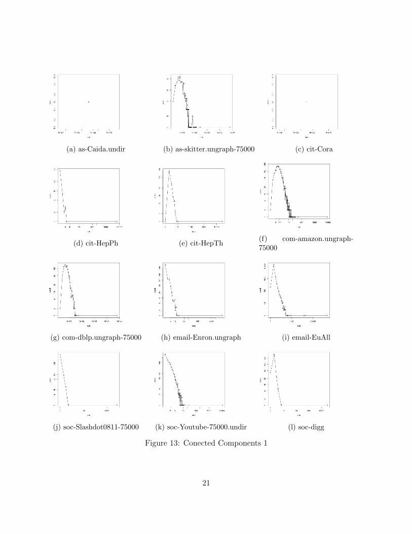
4.2.6 Connected Components

Counts of components of different sizes for individual datasets are plotted in 13 and 14. Anaggregate plot comparing the number of connected components across datasets is shown in12.

Observations

19

Figure 12: Count of connected components in various graphs

1. Most of the graphs have several small components of sizes smaller than 50 and onehuge component that can be seen from the one point at the far right of the graph. Thisseems to be the case with most real-world graphs ([7]).

2. Among the three citation networks, cit-Cora has just 1 connected component whilecit-HepTh and cit-HepPh have 143 and 61 respectively. This suggests disjoint areas ofresearch in the latter two fields, namely theoretical physics. On the other hand, thereexists a path of citations among any two scientists.

3. For the com-amazon and com-dblp datasets and social networks like soc-Youtube andsoc-flickr, the power law relationship among count and size is very prominent forcomponents of low sizes.

4. softjdkdependency dataset also has just 1 weakly connected component, indicating theexistence of chains or hierarchies of dependencies among softwares.

4.2.7 Degree Distribution

Degree distribution plots for individual datasets are plotted in 13 and 14. An aggregate plotcomparing the best-fit power-law exponents across datasets is shown in 15.

Observations

20

(a) as-Caida.undir (b) as-skitter.ungraph-75000 (c) cit-Cora

(d) cit-HepPh (e) cit-HepTh(f) com-amazon.ungraph-75000

(g) com-dblp.ungraph-75000 (h) email-Enron.ungraph (i) email-EuAll

(j) soc-Slashdot0811-75000 (k) soc-Youtube-75000.undir (l) soc-digg

Figure 13: Conected Components 1

21

(a) email-Enron.ungraph (b) email-EuAll (c) soc-pokec-75000

(d) soft-jdkdependency (e) text-spanishbook (f) bio-protein-undir

(g) ca-AstroPh (h) p2p-Gnutella31

Figure 14: Connected Components 2

22

Figure 15: Plot showing magnitude of the power law exponent for count vs degree plot fordifferent datasets

1. For most log-log, degree distribution plots, we observe a linear portion: that is, degreedistributions of real-world graphs approximately follow power laws.

2. In the com-amazon graph, degree distribution following a power law with high exponent(around 3) shows that good products that are usually co-purchased are low in number.

3. We observe a discontinuity in the p2p-Gnutella31 dataset, at the value 10 for degree.The sharp rise suggests that users typically connect to and share files with 10 otherusers at a time.

4. The power-law exponent is in the range 1.8 to 2.3 for most graphs. For email-EuAll,it falls to 1.4, which tells us that even for higher values of degree, the count of verticesdoesn’t fall as rapidly as other datasets. Along with the fact that there are over15000 connected components, this points to the existence of dense clusters, which thentranslates to having small research teams with communication occurring within teams.

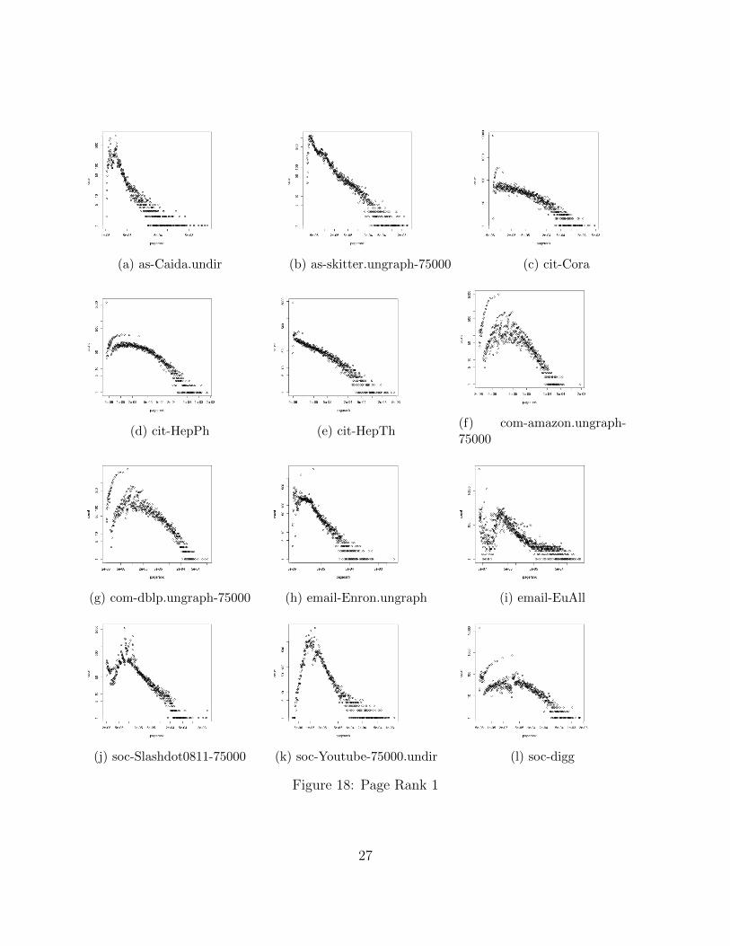
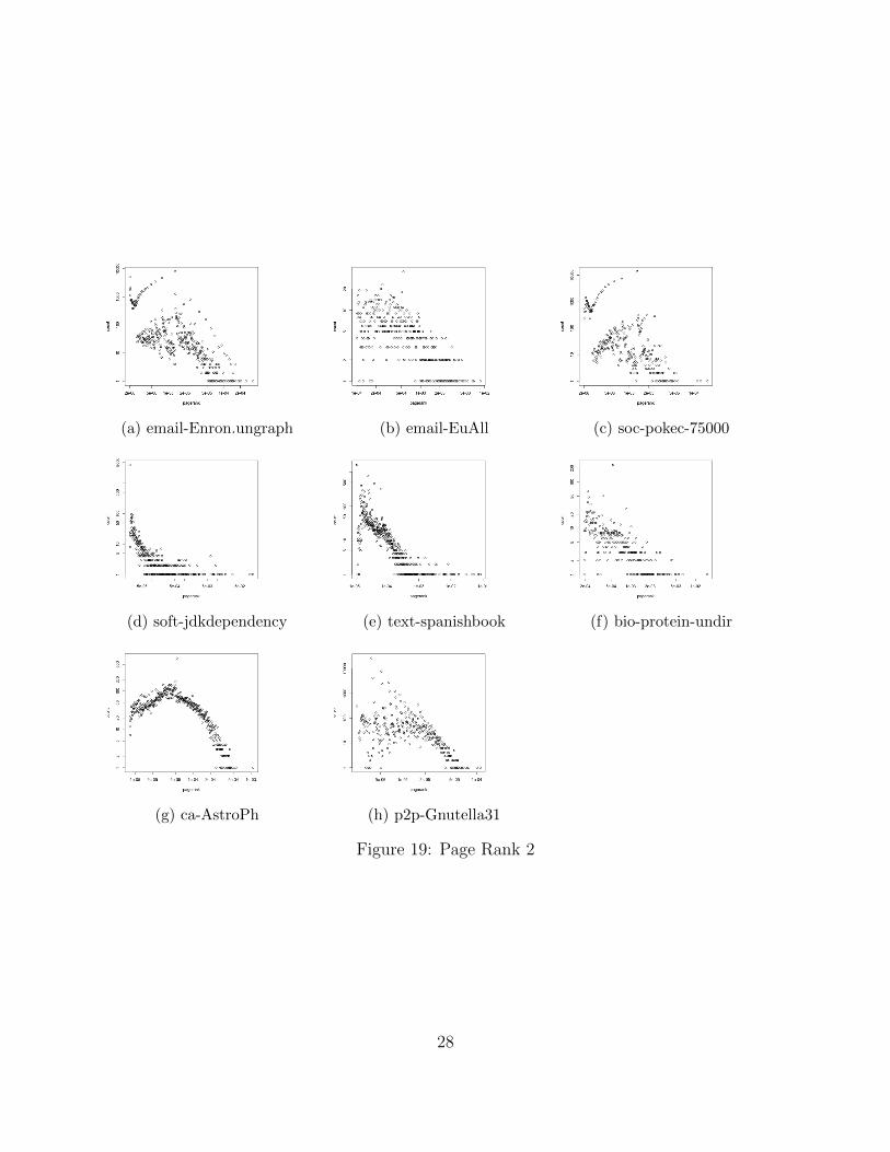
4.2.8 Pagerank

1. Parts of the pagerank-frequency plots in logspace are straight lines, that is, approxi-mately governed by power laws. But these plots do not adhere to the power laws asstrongly as those of degree distribution do.

23





Figure 16: Degree Distribution 1

24




Figure 17: Degree Distribution 2

25

2. Most of the plots have a parabolic beginning, with a power law tail. This is similar tothe behavior of lognormal distributions, as done in class (figures 18 and 19).

3. While graphs such as cit-HepTh have nice straight line plots, some like p2p-Gnutella31and email-EuAll are just scattered all over the place.

4. On the other hand, all 3 co-occurrence graphs: ca-AstroPh, com-amazon and com-dblphave clear parabolic beginning. This could be, as mentioned in class, the parabolicbeginning of a log-normal distribution whose tail follows a power law. See figures 18and 19.

4.2.9 Radius

Radius-count plots for individual datasets are plotted in 21 and 22. An aggregate plotcomparing the maximum effective radii across datasets is shown in 20. Also, radius vs pagerank plots are attached in figure 23.

Observations

1. The maximum radius of most graphs is of the order of 10 to 20.

2. com-amazon gets a value of 50 because the algorithm doesn’t converge, even after 50iterations.

3. It may be noticed that most of the nodes have radii smaller than half the maximum,which means that the real world graphs are pretty closely packed.

4. We also observe a bimodal/unimodal distributions on the radius-count plots. Thisis supported by the observation that was made on the connected components in agraph. The first mode at low radius values comes from nodes belonging to the smallercomponents whose distribution follow a power law. The second mode near the averageradius comes from nodes belonging to the big component. For example, as-skitter ’splot is multi-modal and we can observe from 13 that it has lots of small componentsand 1 big connected component.

4.2.10 Eigenvectors

Notice eigenspokes [13] in figure 24. Observations:

1. The spokes are very clear for datasets as-skitter and the email datasets. This showsthe presence of near cliques or near bipartite cores.

2. The email datasets may have near cliques as departments where everyone sends emailsto almost everyone else.

26





Figure 18: Page Rank 1

27




Figure 19: Page Rank 2

28

Figure 20: Plot showing maximum effective radii for different datasets

3. as-skitter is an internet topology dataset. The eigenspokes may show the presence ofnear-bipartite cores, a bunch of servers and clients.

4.3 Anomaly Detection

Anomaly detection through Egonets was already implemented in the given package. Butthere seems to be some error with this procedure, since having an egonet’s edge-count greaterthan that of a clique is not possible. See figure 25. The black points in the first two plotsrepresent outliers. The third plot seems to be wrong, and doesn’t satisfy sanity checks.

4.4 Heatmaps

Using the datasets provided, we bin up the data so that each set of vertices gets representedby 100 bins. Now, we count the number of edges from each bin to another, and use it as aweight for the heatmap.A few representative plots can be seen in figure 26. The actual outputs can be found in thefolder graphminer/heatmaps/.For example, the heatmaps for cit-HepTh and cit-HepPh strongly indicate the presence ofvery less number of connected components, which is indeed so. On the other hand, theheatmaps for com-amazon and as-skitter datasets show uniform spread, and hence a bigconnected component and many smaller ones, which is true too.

29





Figure 21: Radius 1

30




Figure 22: Radius 2

31

Figure 23: Radius vs Pagerank

32

Figure 24: Eigenvector plots: notice eigenspokes

33

Figure 25: Anomaly detection through Egonets

34

Edge density across bins of vertices

100

101

102

103

104

105

(a) cit-HepPh


100

101

102

103

104

105

(b) cit-HepTh


100

101

102

103

104

(c) as-skitter


100

101

102

103

(d) com-amazon

Figure 26: Heatmaps

35

5 Conclusions

• We have understood and implemented the k-cores algorithm, adding it to the list ofimplemented features.

• We built simple but reliable unit tests, in order to check for sanity of code in futureeasily.

• The algorithms have been run and the results summarized on 22 real-world datasets,showing applicability of the project.

• We have tested various indexing options on the different tables involved in our algo-rithms and studied which ones are a good match.

• After picking the best indices, we have run the algorithms on big datasets and sum-marized the results in this paper.

• We generated plots to depict our results and help simplify analysis.• Based on different parameters like degree-distribution, connected components, etc., we

have attempted to find anomalies and explain features of different datasets.

References

[1] Leman Akoglu and Christos Faloutsos. RTG: A recursive realistic graph generator usingrandom typing. In Machine Learning and Knowledge Discovery in Databases, EuropeanConference, ECML PKDD 2009, Bled, Slovenia, September 7-11, 2009, Proceedings,Part I, pages 13–28, 2009.

[2] Leman Akoglu, Mary Mcglohon, and Christos Faloutsos. Anomaly detection in largegraphs. In In CMU-CS-09-173 Technical Report, 2009.

[3] J. Ignacio Alvarez-Hamelin, Luca Dall’Asta, Alain Barrat, and Alessandro Vespignani.k-core decomposition: a tool for the visualization of large scale networks. CoRR, ab-s/cs/0504107, 2005.

[4] Nijith Jacob and Sharif Doghmi. Graph mining using sql 15-826.

[5] U. Kang, Duen Horng Chau, and Christos Faloutsos. Mining large graphs: Algorithms,inference, and discoveries. In ICDE, pages 243–254, 2011.

[6] U. Kang, Brendan Meeder, and Christos Faloutsos. Spectral analysis for billion-scalegraphs: Discoveries and implementation. In PAKDD (2), pages 13–25, 2011.

[7] U Kang, Charalampos Tsourakakis, and Christos Faloutsos. PEGASUS: A peta-scalegraph mining system - implementation and observations. ICDM, December 2009.

[8] U. Kang, Charalampos E. Tsourakakis, Ana Paula Appel, Christos Faloutsos, and JureLeskovec. Hadi: Mining radii of large graphs. TKDD, 5(2):8, 2011.

36

[9] Danai Koutra, Tai-You Ke, U. Kang, Duen Horng Chau, Hsing-Kuo Kenneth Pao,and Christos Faloutsos. Unifying guilt-by-association approaches: Theorems and fastalgorithms. In ECML/PKDD (2), pages 245–260, 2011.

[10] Milena Mihail and Christos H. Papadimitriou. On the eigenvalue power law. In In-ternational Workshop on Randomization and Approximation Techniques in ComputerScience, Berlin, Germany, 2002. Springer Verlag.

[11] Saket Navlakha, Rajeev Rastogi, and Nisheeth Shrivastava. Graph summarization withbounded error. In Proceedings of the 2008 ACM SIGMOD International Conference onManagement of Data, SIGMOD ’08, pages 419–432, New York, NY, USA, 2008. ACM.

[12] B. Aditya Prakash, Deepayan Chakrabarti, Michalis Faloutsos, Nicholas Valler, andChristos Faloutsos. Got the flu (or mumps)? check the eigenvalue! arXiv:1004.0060v1[physics.soc-ph], 2010.

[13] B. Aditya Prakash, Mukund Seshadri, Ashwin Sridharan, Sridhar Machiraju, and Chris-tos Faloutsos. Eigenspokes: Surprising patterns and scalable community chipping inlarge graphs. PAKDD 2010, 21-24 June 2010.

[14] Jimeng Sun, Huiming Qu, Deepayan Chakrabarti, and Christos Faloutsos. Relevancesearch and anomaly detection in bipartite graphs. KDD Explor. Newsl., 2005.

37

A Appendix

A.1 Labor Division

The team performed the following tasks

• Implementation+Documentation of k-cores [Vipul]• Building Unit-tests 1-4 [Krishna]• Building unit-test 5 [Vipul]• Python code for unit testing [Krishna]• Index-testing [Vipul]• Big-dataset outputs (phase 2) [Krishna]• Big-dataset outputs (phase 3) [Vipul]• Egonet outputs [Krishna]• Individual Dataset Graphs [Krishna]• Aggregate Graphs [Vipul]• Summarization of results + Report generation [both]

38

Contents

1 Introduction 1

2 Survey 22.1 Papers read by Venkata Krishna Pillutla . . . . . . . . . . . . . . . . . . . . 2

2.1.1 Pegasus: Peta-Scale Graph Mining System- Implementation and Ob-servations [7] . . . . . . . . . . . . . . . . . . . . . . . . . . . . . . . 2

2.1.2 Spectral Analysis for Billion-Scale Graphs: Discoveries and Implemen-tation ([6]) . . . . . . . . . . . . . . . . . . . . . . . . . . . . . . . . . 3

2.1.3 Unifying Guilt-by-Association Approaches: Theorems and Fast Algo-rithms ([9]) . . . . . . . . . . . . . . . . . . . . . . . . . . . . . . . . 3

2.2 Papers read by Vipul Singh . . . . . . . . . . . . . . . . . . . . . . . . . . . 42.2.1 k-core decomposition: a tool for the visualization of large scale net-

works ([3]) . . . . . . . . . . . . . . . . . . . . . . . . . . . . . . . . . 42.2.2 Mining Large Graphs: Algorithms, Inference, and Discoveries ([5]) . . 52.2.3 RTG: A Recursive Realistic Graph Generator using Random Typing

([1]) . . . . . . . . . . . . . . . . . . . . . . . . . . . . . . . . . . . . 6

3 Proposed and Implemented Methods 63.1 k-cores . . . . . . . . . . . . . . . . . . . . . . . . . . . . . . . . . . . . . . . 63.2 Unit Tests . . . . . . . . . . . . . . . . . . . . . . . . . . . . . . . . . . . . . 9

4 Experiments 94.1 Phase 1 . . . . . . . . . . . . . . . . . . . . . . . . . . . . . . . . . . . . . . 9

4.1.1 wiki-Vote . . . . . . . . . . . . . . . . . . . . . . . . . . . . . . . . . 104.1.2 soc-Epinions1 . . . . . . . . . . . . . . . . . . . . . . . . . . . . . . . 11

4.2 Phases 2 and 3 . . . . . . . . . . . . . . . . . . . . . . . . . . . . . . . . . . 134.2.1 Indices . . . . . . . . . . . . . . . . . . . . . . . . . . . . . . . . . . . 134.2.2 Indices for connected components and eigen-algorithms . . . . . . . . 144.2.3 Datasets . . . . . . . . . . . . . . . . . . . . . . . . . . . . . . . . . . 154.2.4 5-cores . . . . . . . . . . . . . . . . . . . . . . . . . . . . . . . . . . . 154.2.5 Eigen-triangle count . . . . . . . . . . . . . . . . . . . . . . . . . . . 184.2.6 Connected Components . . . . . . . . . . . . . . . . . . . . . . . . . 194.2.7 Degree Distribution . . . . . . . . . . . . . . . . . . . . . . . . . . . . 204.2.8 Pagerank . . . . . . . . . . . . . . . . . . . . . . . . . . . . . . . . . 234.2.9 Radius . . . . . . . . . . . . . . . . . . . . . . . . . . . . . . . . . . . 264.2.10 Eigenvectors . . . . . . . . . . . . . . . . . . . . . . . . . . . . . . . . 26

4.3 Anomaly Detection . . . . . . . . . . . . . . . . . . . . . . . . . . . . . . . . 294.4 Heatmaps . . . . . . . . . . . . . . . . . . . . . . . . . . . . . . . . . . . . . 29

5 Conclusions 36

i

A Appendix 38A.1 Labor Division . . . . . . . . . . . . . . . . . . . . . . . . . . . . . . . . . . 38

ii

v mine graphs

Documents