V5R4 SQL Packs a Punch - Kent Milligan Originally published in March 2006 issue of iSeries Network magazine Most new releases of DB2 UDB for iSeries include incremental SQL enhancements such as new data types and built-in functions. V5R4 is no different in that regard, with new built-in functions for Triple DES encryption, date processing, and sampling functions. DB2 UDB for iSeries in V5R4, however, differentiates itself with support for recursive SQL and online analytical processing (OLAP) expressions. These powerful features will help programmers solve many business problems, such as bill of materials processing.

Note that the V5R4 SQL features I discuss here are supported only by the SQL Query Engine (SQE). This means that if your environment or SQL request contains an attribute that is not supported by SQE and you’re trying to use one of these new SQL features, DB2 UDB will flag an error.

Here’s a list of some of the more common items that prevent SQE from running an SQL request:

· Use of UPPER, LOWER, or TRANSLATE function · National Language Sort Sequence · User-Defined Table Function (UDTF) · Logical File references on FROM clause · Select/Omit Logical Files defined on underlying table For more details on SQE support, visit ibm.com/iseries/db2/sqe.html RANKing your Results When you’re ordering the results of a query, it often would be nice to apply a ranking to highlight another data attribute. For example, returning a list of sales persons ordered by their last name and including their rankings in terms of total revenue. Figure 1 shows a sample query to reveal the syntax in action.

SELECT position, last_name, batting_avg, RANK() OVER(ORDER BY batting_avg DESC) AS ba_rank FROM players WHERE team=’REDS’ and position<>’P’ ORDER BY last_name

Figure 1

The Order By clause in this query causes the list of baseball players to appear in alphabetic order, so it’s easy to find a player. The OLAP expression Rank() allows for a secondary ordering to be specified on the Select statement using the new OVER keyword. This secondary ordering (i.e., OVER(ORDER BY batting_avg DESC)) is used to generate the ranking criteria for the result set.

In this case, the batting average ranking for each player is included in the final result, rating the players by their batting average from highest to lowest. The ranking makes it easy to identify the top hitters in the list as demonstrated in the query output in Figure 2.

The value being ranked does not have to be limited to a single column. The Order By specified in then Over clause supports all of the capabilities of a regular Order By clause (e.g., expressions, multiple columns).

There is actually a second ranking expression known as Dense_Rank. Rank and Dense_Rank behave in an almost identical fashion, except when the values being ranked contain duplicate values. If you look at the results in Figure 2 closely, you will see that two of the lower ranked hitters (Perez and Foster) actually had the same batting average and thus shared the same ranking. In this case, the Rank expression caused a gap in the ranking by skipping from 6 to 8 because of the tie at the sixth ranking slot.

Figure 2

If you run the same query again with the Dense_Rank expression, you will see from the query output in Figure 3 that Dense_Rank does not have a gap in its ranking. Geronimo and Perez share a ranking of 6 and Concepcion’s ranking is moved up to 7.

Figure 3 Next Number Please Many times, iSeries programmers also want the ability to arbitrarily number the rows returned by a query to have an easy way of identifying the rows in a result set. The new Row_Number expression in V5R4 provides exactly that capability. The code in Figure 4, which produces the results in Figure 5, demonstrates this.

SELECT ROW_NUMBER() OVER (ORDER BY workdept, lastname) AS Nbr, lastname, salary FROM employee ORDER BY workdept, lastname

Figure 4

Figure 5

The Row_Number expression does not compare the values of any

columns like the ranking expressions. Instead, Row_number simply generates the next row number and assigns it to the next sequential row based on the ordering criteria on the Over clause. The Order By clause is optional. However, if an Order By clause is not specified the row_number, values will be assigned based on how DB2 UDB returns the results of the SELECT statement back to the application. In the above code, the Order By clause can be dropped from the Row_Number expression because the SELECT statement orders the results data in the same way. If your application needs the ability to restart this arbitrary row number for a subset or sub-grouping of the results, the Row_Number expression has a partitioning clause that fills this need, as the statement in Figure 6 shows.

SELECT workdept, lastname, hiredate, ROW_NUMBER() OVER (PARTITION BY workdept ORDER BY hiredate) AS Nbr FROM employee ORDER BY workdept, hiredate

Figure 6

In this query, the row number is generated and assigned based on sorting by the employee’s department number and last name. The Partition By clause, however, causes the row number to be restarted each time that a new department (i.e, the partitioning column) is encountered in the result set. This resetting of the row number is easily observed in the output produced by this query (Figure 7).

Figure 7 The Power of Expression Not only can you use the Row_Number expression to assign an identifier, but you can also use it to simply process a subset of a result set. In the example in Figure 8, the Row_Number expression is used in conjunction with a common table expression (i.e., the WITH clause) to return (in Figure 9) only a subset of the employees from the previous example.

WITH numbering AS ( SELECT ROW_NUMBER() OVER (ORDER BY workdept,lastname) AS rowno, lastname, salary, workdept FROM emp) SELECT rowno, lastname, salary FROM numbering WHERE rowno BETWEEN 6 AND 10 ORDER BY workdept, lastname

Figure 8

Figure 9

If this is your first encounter with a common table expression (CTE), just think if of as creating a temporary SQL view that can be

used only by the associated SELECT statement. The numbering table expression assigns an identifier to each employee, and then the SELECT statement specifies which range or set of employees to return. The constant values in this statement, 6 and 10, could be replaced with parameter markers or host variables to allow the application to use this statement to page through or grab a different subset of results using the same query.

You might be thinking that this statement is overly complex with the numbering common table expression and that the table expression could be dropped to produce a simpler version:

SELECT ROW_NUMBER() OVER (ORDER BY workdept, lastname) AS rowno, lastname, salary, workdept FROM emp WHERE rowno BETWEEN 6 AND 10 ORDER BY workdept, lastname

However, this is not allowed by the SQL standard because the

WHERE clause is processed before the expressions on the SELECT list. Consequently, the rowno reference on the WHERE clause will be flagged as an undefined column because the DB2 SQL parser has not processed the rowno expression defined on the SELECT list.

In Figure 8, a common table expression (i.e., the WITH clause) was used to define rowno before the main SELECT statement. Thus, common table expressions are a very useful tool when you want to reuse complex calculations or expressions on different clauses of a single SQL statement. Embedding the Row_Number in an SQL View is another option, but the tradeoff is that you have two separate SQL statements. Recursion, Recursion, Recursion DB2 UDB has actually supported CTEs for iSeries since V4R4. With V5R4, CTEs have become an even more useful and powerful SQL feature, with the ability to perform recursive processing. A common table expression that includes a recursive reference is known as a recursive common table expression (RCTE). You are probably thinking that recursive SQL is for computer science geeks and not a useful tool for solving business problems. However, you should analyze your databases before coming to that conclusion. Many database tables contain rows that have an inherent relationship to other rows in the same table, such as organizational hierarchies, bill-of-materials, or travel connections that are naturally navigated with recursive algorithms. An easy business problem that I can use to explain an RCTE is the hierarchical relationships that exist in a company’s organizational chart (Figure 10). The company’s president (Olson) wants to know all the employees that work for a middle manager named Carfino. This list of employees must include not only Carfino’s immediate reports, but also the people that work for those managers. If the request was just for Carfino’s immediate reports, than a simple SQL query could solve the problem. Yet, the president’s demand requires navigating through all of the management layers in the company.

Figure 10

You could provide a solution by using an iterative manual

approach whereby an application runs a query to find the immediate reports and then stores that information away before looping through again to find the employees that work for Carfino’s immediate reports, and so on. On the other hand, this is the perfect situation to use recursive SQL. An RCTE provides simple navigation through all the management layers with a single SQL request. From the recursive example in Figure 11, you need to see that a RCTE is composed of three different phases. Each phase is differentiated in Figure 11 with a different color. These phases are: · Initializing the query (in green) · Recursively navigating to the next level (in blue) · Kicking off the recursion and returning the final results (in red)

CREATE TABLE emp( empid INTEGER PRIMARY KEY, name VARCHAR(10), salary DECIMAL(9, 2), mgrid INTEGER) WITH emp_list (level, empid, name) AS (SELECT 1, empid, name FROM emp WHERE name = 'Carfino' UNION ALL SELECT o.level + 1, next_layer.empid, next_layer.name FROM emp as next_layer, emp_list o WHERE o.empid = next_layer.mgrid ) SELECT level, name FROM emp_list

Figure 11

In this RCTE example, the initialization phase must help identify

all the employees that work directly for Carfino. Thus, the first step is retrieving Carfino’s employee ID, so that the next phase can find

Olson

Lester

Davis Armstrong

Carfino

Stokes Payne

Brookins Horton Lohaus Horner Brunner

Bullard Settles

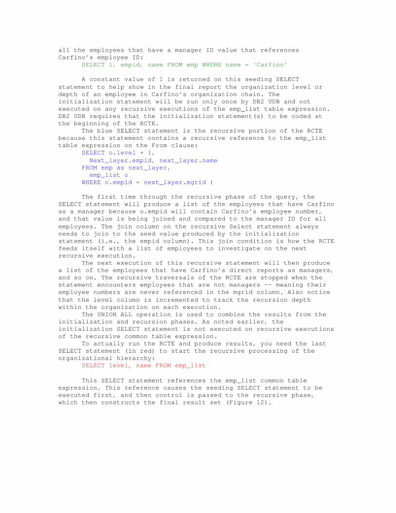
all the employees that have a manager ID value that references Carfino’s employee ID:

SELECT 1, empid, name FROM emp WHERE name = 'Carfino'

A constant value of 1 is returned on this seeding SELECT statement to help show in the final report the organization level or depth of an employee in Carfino’s organization chain. The initialization statement will be run only once by DB2 UDB and not executed on any recursive executions of the emp_list table expression. DB2 UDB requires that the initialization statement(s) to be coded at the beginning of the RCTE. The blue SELECT statement is the recursive portion of the RCTE because this statement contains a recursive reference to the emp_list table expression on the From clause:

SELECT o.level + 1, Next_layer.empid, next_layer.name FROM emp as next_layer, emp_list o WHERE o.empid = next_layer.mgrid )

The first time through the recursive phase of the query, the

SELECT statement will produce a list of the employees that have Carfino as a manager because o.empid will contain Carfino’s employee number, and that value is being joined and compared to the manager ID for all employees. The join column on the recursive Select statement always needs to join to the seed value produced by the initialization statement (i.e., the empid column). This join condition is how the RCTE feeds itself with a list of employees to investigate on the next recursive execution.

The next execution of this recursive statement will then produce a list of the employees that have Carfino’s direct reports as managers, and so on. The recursive traversals of the RCTE are stopped when the statement encounters employees that are not managers –- meaning their employee numbers are never referenced in the mgrid column. Also notice that the level column is incremented to track the recursion depth within the organization on each execution.

The UNION ALL operation is used to combine the results from the initialization and recursion phases. As noted earlier, the initialization SELECT statement is not executed on recursive executions of the recursive common table expression. To actually run the RCTE and produce results, you need the last SELECT statement (in red) to start the recursive processing of the organizational hierarchy:

SELECT level, name FROM emp_list

This SELECT statement references the emp_list common table expression. This reference causes the seeding SELECT statement to be executed first, and then control is passed to the recursive phase, which then constructs the final result set (Figure 12).

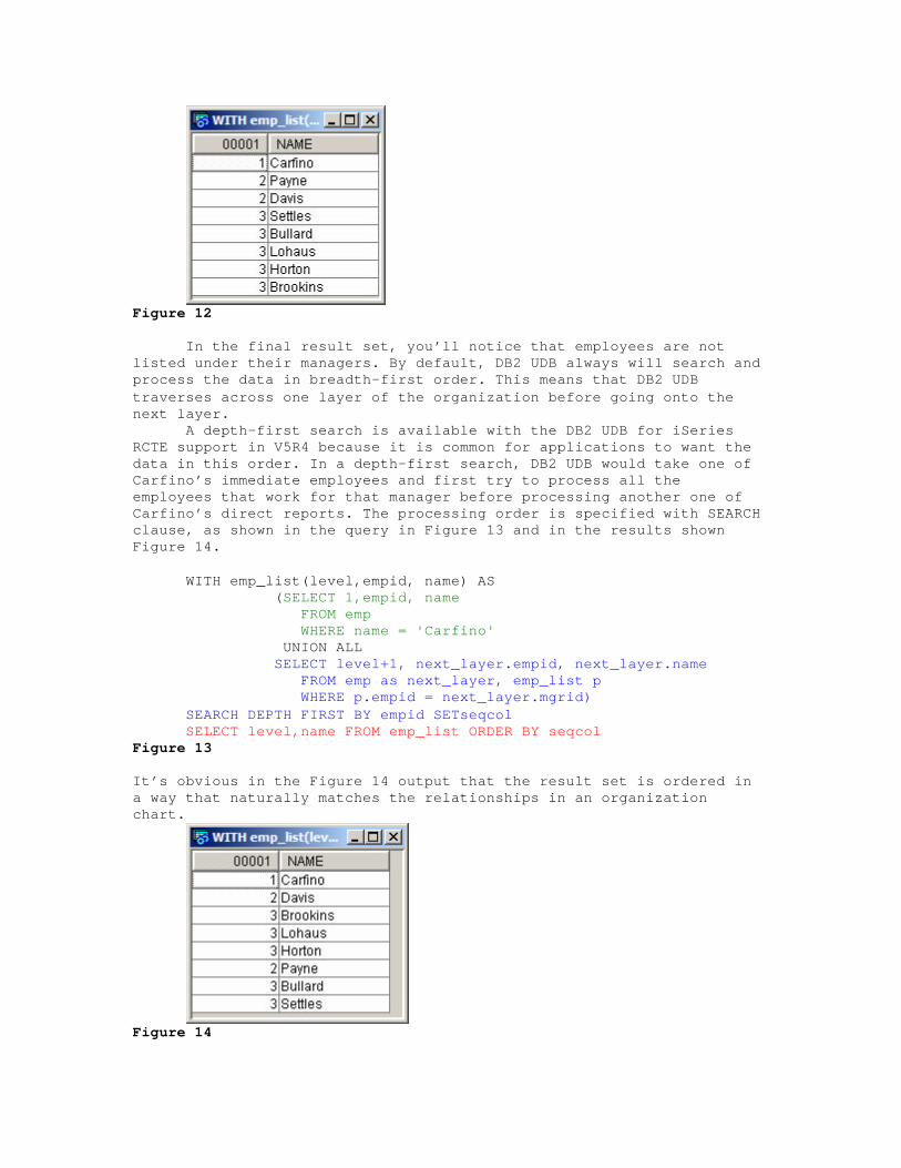
Figure 12

In the final result set, you’ll notice that employees are not

listed under their managers. By default, DB2 UDB always will search and process the data in breadth-first order. This means that DB2 UDB traverses across one layer of the organization before going onto the next layer. A depth-first search is available with the DB2 UDB for iSeries RCTE support in V5R4 because it is common for applications to want the data in this order. In a depth-first search, DB2 UDB would take one of Carfino’s immediate employees and first try to process all the employees that work for that manager before processing another one of Carfino’s direct reports. The processing order is specified with SEARCH clause, as shown in the query in Figure 13 and in the results shown Figure 14.

WITH emp_list(level,empid, name) AS (SELECT 1,empid, name FROM emp WHERE name = 'Carfino' UNION ALL SELECT level+1, next_layer.empid, next_layer.name FROM emp as next_layer, emp_list p WHERE p.empid = next_layer.mgrid) SEARCH DEPTH FIRST BY empid SETseqcol SELECT level,name FROM emp_list ORDER BY seqcol

Figure 13 It’s obvious in the Figure 14 output that the result set is ordered in a way that naturally matches the relationships in an organization chart.

Figure 14

The first thing to notice in this Depth First example is that the SEARCH clause needs to use the same column that’s specified on the recursive join reference –- in this case, empid. In addition to this navigation column, the SEARCH clause also contains a Set keyword with another column name -- SeqCol. DB2 UDB uses this column to keep track of the order that it visited the rows on this SQL request. The sequencing column specified on the SET is very important because this same column name must also be specified on the ORDER BY clause. The column name itself is not important, so you’re free to choose any name. If this sequencing column is not referenced on the ORDER BY clause, then DB2 UDB ignores the entire SEARCH clause. Remember that with SQL, if you want to return your data in a specific order, an ORDER BY clause is the only way to guarantee that ordering. If the president has just requested this list of employees under Carfino so he could send out a congratulatory e-mail for a recent project success, than there is no need to specify a search clause and slow down the DB2 UDB recursive processing. If the president was new to the company and was unsure of Carfino’s organizational chain, then the application should specify the Search and Order by clause to return the employees in a depth-first order, as Figure 14 shows. You will get the best performance with RCTEs when the search clause is not specified. Only include this clause if you need to control the processing order when a specific order of the data relationships or hierarchies is truly required by the application. There’s actually one part of a recursive common table expression that I haven’t discussed yet, and that’s the Cycle clause. There are some cases where your tables may contain recursive data relationships that are cyclical or never-ending. In an organization hierarchy, you don’t have to worry about getting into a never-ending cycle because you don’t have many company presidents that report to entry-level employees at the bottom of the organization. On the other hand, let’s consider a table such as the Flights table in Figure 15, which contains the air flight combinations for a set of cities. Here is the SQL table definition that corresponds to Figure 15:

CREATE TABLE flights (departure VARCHAR(40), arrival VARCHAR(40), carrier CHAR(20))

Figure 15

Say you’re going to write a recursive SQL request that figures out all of the destinations that you can get to from a starting city, such as Rochester. In this case, your recursive SQL request will need to be concerned about finding a destination such as Minneapolis that also has a direct flight to Rochester. If the SQL statement doesn’t detect that a starting point of Rochester caused the query to traverse

Departure City Arrival City Carrier Rochester Chicago FlyCheap Chicago New York Eastern Air Chicago Seattle Westward Ho Chicago Minneapolis Central Air Minneapolis Rochester Central Air Minneapolis Detroit Central Air

to a Rochester destination, the query will go into an infinite loop. That’s exactly the support provided by the Cycle clause the SQL query in Figure 16 shows.

WITH destinations (departure,arrival,itinerary)AS (SELECT f.departure,f.arrival, CAST (f.departure ||’->’|| f.arrival AS VARCHAR(200)) FROM flights f WHERE f.departure =’Rochester’ UNION ALL SELECT r.departure,b.arrival, CAST (r.itinerary ||’->’|| b.arrival AS VARCHAR(200)) FROM destinations r,flights b WHERE r.arrival =b.departure ) CYCLE arrival SET cyclic_data TO ’1 ’ DEFAULT ’0 ’ SELECT departure,arrival,itinerary,cyclic_data FROM destinations

Figure 16

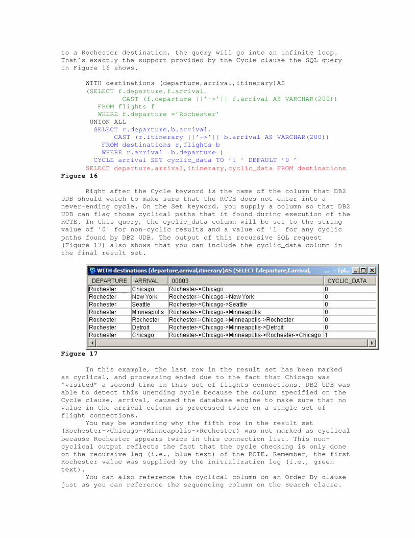
Right after the Cycle keyword is the name of the column that DB2 UDB should watch to make sure that the RCTE does not enter into a never-ending cycle. On the Set keyword, you supply a column so that DB2 UDB can flag those cyclical paths that it found during execution of the RCTE. In this query, the cyclic_data column will be set to the string value of '0' for non-cyclic results and a value of '1' for any cyclic paths found by DB2 UDB. The output of this recursive SQL request (Figure 17) also shows that you can include the cyclic_data column in the final result set.

Figure 17 In this example, the last row in the result set has been marked as cyclical, and processing ended due to the fact that Chicago was “visited” a second time in this set of flights connections. DB2 UDB was able to detect this unending cycle because the column specified on the Cycle clause, arrival, caused the database engine to make sure that no value in the arrival column is processed twice on a single set of flight connections.

You may be wondering why the fifth row in the result set (Rochester->Chicago->Minneapolis->Rochester) was not marked as cyclical because Rochester appears twice in this connection list. This non-cyclical output reflects the fact that the cycle checking is only done on the recursive leg (i.e., blue text) of the RCTE. Remember, the first Rochester value was supplied by the initialization leg (i.e., green text).

You can also reference the cyclical column on an Order By clause just as you can reference the sequencing column on the Search clause.

Furthermore, you can choose any column name for the cyclical column. You have some freedom in choosing the values assigned to the cyclical column, but you are limited to values that are character strings one byte in length. The key here is to remember to include the Cycle clause when cyclical data may exist in your tables to prevent never-ending recursive SQL requests.

Recursive Explosions While an organization chart or flight planner may be good at demonstrating the concepts of recursive SQL, you may still be skeptical as to whether RCTEs can solve real business problems. I’ll use a bill-of-materials example here because iSeries servers are often used in the manufacturing and distribution industries. In fact, let’s use a RCTE to explode the bill of materials (BOM) for an iSeries Power5 server. In this BOM example, there are two tables: CREATE TABLE materials (prod_bom_id CHAR(4) --parent part, prod_id CHAR(4), quantity INTEGER); CREATE TABLE products (prod_id CHAR(4), product_name VARCHAR(30));

The materials table has contains all the part relationships for all the different components used in an iSeries server (e.g., processors, memory). The products table stores a descriptive name for of each part and product. Next, let’s examine the RCTE bom (Figure 18), which will be used to navigate all the components that make up an iSeries Power5 Server. The initialization leg specifies a part type of 9406 to find the top level of server components. Notice the initialization leg contains a constant value of 1 to track the nesting of each part and a join against the products table, so that the output can include the descriptive name for each component instead of a cryptic part number. The recursive leg increments the level tracker, performs the same join to drag along the product name, and then retrieves the next level of components to feed the RCTE.

WITH bom (level, part, description, qty) AS (SELECT 1, m.prod_id, product_name, quantity FROM materials m, products p WHERE m.prod_id=p.prod_id AND prod_bom_id='9406' UNION ALL SELECT level+1, next_level.prod_id, product_name, quantity FROM materials next_level, bom parent, products pd WHERE parent.part = next_level.prod_bom_id AND next_level.prod_id=pd.prod_id) SEARCH DEPTH FIRST BY part SET seqcol SELECT level , part, qty, description FROM bom ORDER BY seqcol

Figure 18 The SEARCH clause is included to specify a depth-first search, so that the output can nest together the related parts, as Figure 19

shows. For example, Figure 19 shows the Disk Units (4326) as a subcomponent of the Storage Controller (5709).

If you want to include the owning part number in the final report

so that’s it even easier to see the server component relationships, you can just modify the query, as in Figure 20. Figure 21 shows the results of this modification. The Final Scorecard Hopefully, you now see clearly how the V5R4 support for the Rank and RowNumber OLAP expressions, along with recursive table expressions, bring the DB2 UDB for iSeries SQL to a brand new level of capability. Even more importantly, you hopefully understand how to use these SQL enhancements to knock out your next business problem. Kent Milligan is a DB2 UDB of for i5/OS consultant in ISV Enablement for System i.