variance reduction's greatest hits - accueillecuyer/lecce09/lecce09-s4b.pdf · 1 variance...
TRANSCRIPT

1
Variance Reduction’s Greatest Hits
Pierre L’Ecuyer
CIRRELT, GERAD, andDepartement d’Informatique et de Recherche Operationnelle
Universite de Montreal, Canada
ESM 2007, Malta, October 22, 2007

2
Context
Some steps in a stochastic simulation project:
I Define purpose of project;
I System and data collection/examination;
I Build a mathematical model;
I Define estimators and algorithms;
I Prepare and organize all the required software;
I Run simulations until satisfied;
I Analyze and use results; Possible feedback on previous steps.
3
Outline
1. Monte Carlo.
2. Importance of improving efficiency of estimators.
3. Common random numbers (CRN).
4. Importance sampling (IS).
5. Control variates (CV).
6. Conditional Monte Carlo (CMC).
7. Generalized antithetic variates andrandomized quasi-Monte Carlo (RQMC).
8. Conclusion.
4
Monte Carlo and efficiency of estimators
In stochastic simulation models, we often want to estimate themathematical expectation (an average) of some random variable X :
µ = E[X ].
For example, X can be
I the net discounted payoff of some financial option;
I the amount of pollution (or profit, or other type of output)produced by some factory on a given month;
I the number of calls answered after more than 20 seconds,on a given day, in a call center; and so on.
For one realization of X , we may have to run a complicated simulationprogram that takes several minutes or even hours to execute, and usesmillions (or more) of random numbers.
5
Monte Carlo
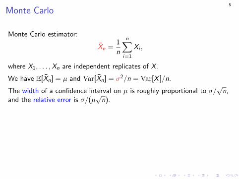
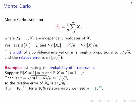
Monte Carlo estimator:
Xn =1
n
n∑i=1
Xi ,
where X1, . . . ,Xn are independent replicates of X .
We have E[Xn] = µ and Var[Xn] = σ2/n = Var[X ]/n.
The width of a confidence interval on µ is roughly proportional to σ/√
n,and the relative error is σ/(µ
√n).
Example: estimating the probability of a rare event.Suppose P[X = 1] = µ and P[X = 0] = 1− µ.Then σ/µ =
√µ(1− µ)/µ ≈ 1/
õ,
so the relative error of Xn is 1/√
nµ.If µ = 10−10, for a 10% relative error, we need n = 1012.
5
Monte Carlo
Monte Carlo estimator:
Xn =1
n
n∑i=1
Xi ,
where X1, . . . ,Xn are independent replicates of X .
We have E[Xn] = µ and Var[Xn] = σ2/n = Var[X ]/n.
The width of a confidence interval on µ is roughly proportional to σ/√
n,and the relative error is σ/(µ
√n).
Example: estimating the probability of a rare event.Suppose P[X = 1] = µ and P[X = 0] = 1− µ.Then σ/µ =
√µ(1− µ)/µ ≈ 1/
õ,
so the relative error of Xn is 1/√
nµ.If µ = 10−10, for a 10% relative error, we need n = 1012.
6
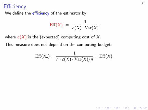
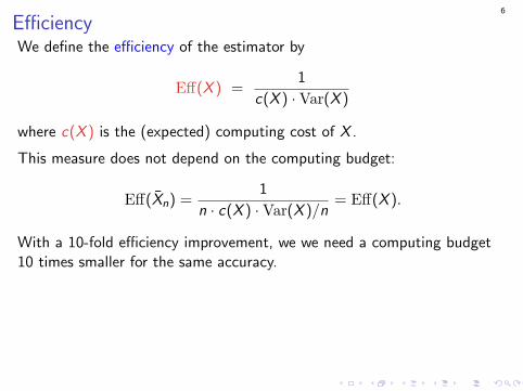
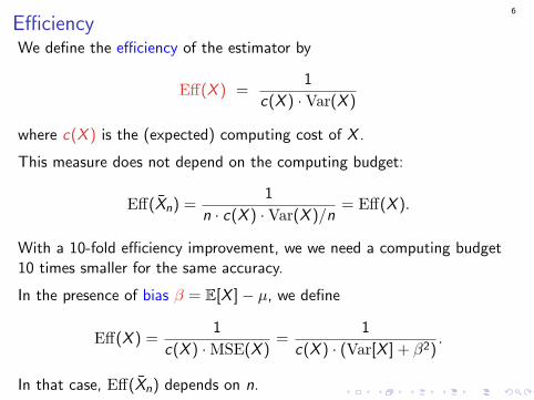
EfficiencyWe define the efficiency of the estimator by
Eff(X ) =1
c(X ) ·Var(X )
where c(X ) is the (expected) computing cost of X .
This measure does not depend on the computing budget:
Eff(Xn) =1
n · c(X ) ·Var(X )/n= Eff(X ).
With a 10-fold efficiency improvement, we we need a computing budget10 times smaller for the same accuracy.
In the presence of bias β = E[X ]− µ, we define
Eff(X ) =1
c(X ) ·MSE(X )=
1
c(X ) · (Var[X ] + β2).
In that case, Eff(Xn) depends on n.
6
EfficiencyWe define the efficiency of the estimator by
Eff(X ) =1
c(X ) ·Var(X )
where c(X ) is the (expected) computing cost of X .
This measure does not depend on the computing budget:
Eff(Xn) =1
n · c(X ) ·Var(X )/n= Eff(X ).
With a 10-fold efficiency improvement, we we need a computing budget10 times smaller for the same accuracy.
In the presence of bias β = E[X ]− µ, we define
Eff(X ) =1
c(X ) ·MSE(X )=
1
c(X ) · (Var[X ] + β2).
In that case, Eff(Xn) depends on n.
7
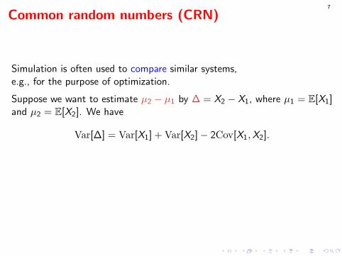
Common random numbers (CRN)
Simulation is often used to compare similar systems,e.g., for the purpose of optimization.
Suppose we want to estimate µ2 − µ1 by ∆ = X2 − X1, where µ1 = E[X1]and µ2 = E[X2]. We have
Var[∆] = Var[X1] + Var[X2]− 2Cov[X1,X2].
If each Xk has (fixed) cdf Fk for k = 1, 2, then taking Xk = F−1k (U) for a
single common r.v. U ∼ U(0, 1) maximizes the covariance (Frechet 1951).
For typical simulations, F−1k (U) is much too complicated to compute.
7
Common random numbers (CRN)
Simulation is often used to compare similar systems,e.g., for the purpose of optimization.
Suppose we want to estimate µ2 − µ1 by ∆ = X2 − X1, where µ1 = E[X1]and µ2 = E[X2]. We have
Var[∆] = Var[X1] + Var[X2]− 2Cov[X1,X2].
If each Xk has (fixed) cdf Fk for k = 1, 2, then taking Xk = F−1k (U) for a
single common r.v. U ∼ U(0, 1) maximizes the covariance (Frechet 1951).
For typical simulations, F−1k (U) is much too complicated to compute.
8
Common random numbers
What we can do is simulate the two systems with exactly the samestreams of uniforms random numbers. Important: make sure that thecommon random numbers (CRN) are used for the same purpose for bothsystems (synchronization) and generate all r.v.’s by inversion.
Proposition. If X1 and X2 are monotone functions of each uniform, in thesame direction then Cov[X1,X2] > 0.
Multiple comparisons: All of this applies if we want to compare severalsimilar systems.
8
Common random numbers
What we can do is simulate the two systems with exactly the samestreams of uniforms random numbers. Important: make sure that thecommon random numbers (CRN) are used for the same purpose for bothsystems (synchronization) and generate all r.v.’s by inversion.
Proposition. If X1 and X2 are monotone functions of each uniform, in thesame direction then Cov[X1,X2] > 0.Multiple comparisons: All of this applies if we want to compare severalsimilar systems.

9
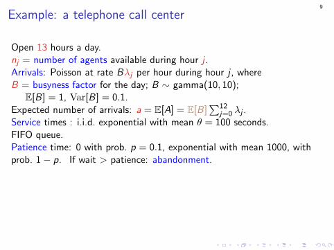
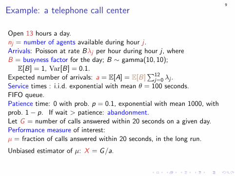
Example: a telephone call center
Open 13 hours a day.nj = number of agents available during hour j .Arrivals: Poisson at rate Bλj per hour during hour j , whereB = busyness factor for the day; B ∼ gamma(10, 10);
E[B] = 1, Var[B] = 0.1.Expected number of arrivals: a = E[A] = E[B]
∑12j=0 λj .
Service times : i.i.d. exponential with mean θ = 100 seconds.FIFO queue.Patience time: 0 with prob. p = 0.1, exponential with mean 1000, withprob. 1− p. If wait > patience: abandonment.Let G = number of calls answered within 20 seconds on a given day.Performance measure of interest:µ = fraction of calls answered within 20 seconds, in the long run.
Unbiased estimator of µ: X = G/a.
9
Example: a telephone call center
Open 13 hours a day.nj = number of agents available during hour j .Arrivals: Poisson at rate Bλj per hour during hour j , whereB = busyness factor for the day; B ∼ gamma(10, 10);
E[B] = 1, Var[B] = 0.1.Expected number of arrivals: a = E[A] = E[B]
∑12j=0 λj .
Service times : i.i.d. exponential with mean θ = 100 seconds.FIFO queue.Patience time: 0 with prob. p = 0.1, exponential with mean 1000, withprob. 1− p. If wait > patience: abandonment.
Let G = number of calls answered within 20 seconds on a given day.Performance measure of interest:µ = fraction of calls answered within 20 seconds, in the long run.
Unbiased estimator of µ: X = G/a.
9
Example: a telephone call center
Open 13 hours a day.nj = number of agents available during hour j .Arrivals: Poisson at rate Bλj per hour during hour j , whereB = busyness factor for the day; B ∼ gamma(10, 10);
E[B] = 1, Var[B] = 0.1.Expected number of arrivals: a = E[A] = E[B]
∑12j=0 λj .
Service times : i.i.d. exponential with mean θ = 100 seconds.FIFO queue.Patience time: 0 with prob. p = 0.1, exponential with mean 1000, withprob. 1− p. If wait > patience: abandonment.Let G = number of calls answered within 20 seconds on a given day.Performance measure of interest:µ = fraction of calls answered within 20 seconds, in the long run.
Unbiased estimator of µ: X = G/a.
10
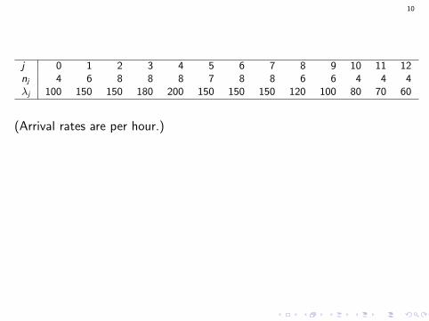
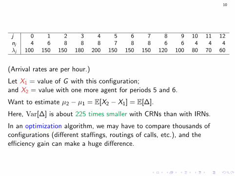
j 0 1 2 3 4 5 6 7 8 9 10 11 12nj 4 6 8 8 8 7 8 8 6 6 4 4 4λj 100 150 150 180 200 150 150 150 120 100 80 70 60
(Arrival rates are per hour.)
Let X1 = value of G with this configuration;and X2 = value with one more agent for periods 5 and 6.
Want to estimate µ2 − µ1 = E[X2 − X1] = E[∆].
Here, Var[∆] is about 225 times smaller with CRNs than with IRNs.
In an optimization algorithm, we may have to compare thousands ofconfigurations (different staffings, routings of calls, etc.), and theefficiency gain can make a huge difference.
10
j 0 1 2 3 4 5 6 7 8 9 10 11 12nj 4 6 8 8 8 7 8 8 6 6 4 4 4λj 100 150 150 180 200 150 150 150 120 100 80 70 60
(Arrival rates are per hour.)
Let X1 = value of G with this configuration;and X2 = value with one more agent for periods 5 and 6.
Want to estimate µ2 − µ1 = E[X2 − X1] = E[∆].
Here, Var[∆] is about 225 times smaller with CRNs than with IRNs.
In an optimization algorithm, we may have to compare thousands ofconfigurations (different staffings, routings of calls, etc.), and theefficiency gain can make a huge difference.
11
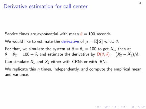
Derivative estimation for call center
Service times are exponential with mean θ = 100 seconds.
We would like to estimate the derivative of µ = E[G ] w.r.t. θ.
For that, we simulate the system at θ = θ1 = 100 to get X1, then atθ = θ2 = 100 + δ, and estimate the derivative by D(θ, δ) = (X2 − X1)/δ.
Can simulate X1 and X2 either with CRNs or with IRNs.
We replicate this n times, independently, and compute the empirical meanand variance.

12
How to implement CRNs?
Four types of random variates in this model, all generated by inversion:
(a) the busyness factor B for the day;(b) the times between successive arrivals of calls;(c) the call durations;(d) the patience times;
Synchronization problem: when service times change, waiting times andabandonment decisions can change.For a given call, we may need to generate a patience time in one case andnot on the other one (if call does not wait), or a service time in one caseand not on the other one (if call abandons).

13
Possible strategies:
(a) generate a service time for all calls, or
(b) only for those who do not abandon.
Similarly, we can
(c) generate a patience time for all calls, or
(d) only for those who wait.

13
Possible strategies:
(a) generate a service time for all calls, or
(b) only for those who do not abandon.
Similarly, we can
(c) generate a patience time for all calls, or
(d) only for those who wait.
14
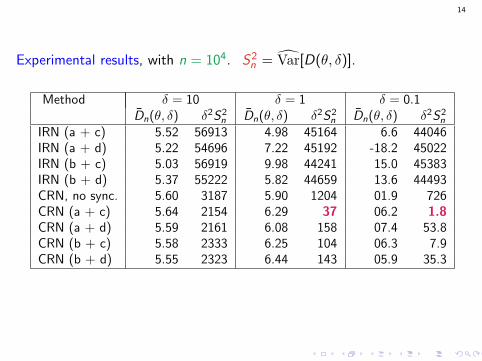
Experimental results, with n = 104. S2n = Var[D(θ, δ)].
Method δ = 10 δ = 1 δ = 0.1Dn(θ, δ) δ2S2
n Dn(θ, δ) δ2S2n Dn(θ, δ) δ2S2
n
IRN (a + c) 5.52 56913 4.98 45164 6.6 44046IRN (a + d) 5.22 54696 7.22 45192 -18.2 45022IRN (b + c) 5.03 56919 9.98 44241 15.0 45383IRN (b + d) 5.37 55222 5.82 44659 13.6 44493CRN, no sync. 5.60 3187 5.90 1204 01.9 726CRN (a + c) 5.64 2154 6.29 37 06.2 1.8CRN (a + d) 5.59 2161 6.08 158 07.4 53.8CRN (b + c) 5.58 2333 6.25 104 06.3 7.9CRN (b + d) 5.55 2323 6.44 143 05.9 35.3

15
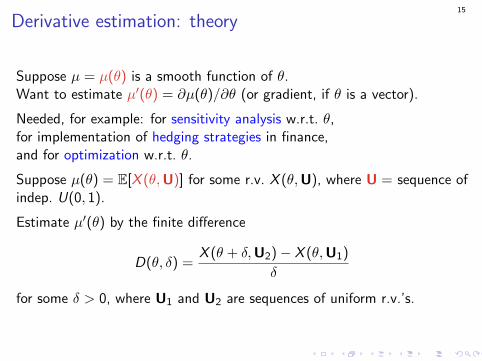
Derivative estimation: theory
Suppose µ = µ(θ) is a smooth function of θ.Want to estimate µ′(θ) = ∂µ(θ)/∂θ (or gradient, if θ is a vector).
Needed, for example: for sensitivity analysis w.r.t. θ,for implementation of hedging strategies in finance,and for optimization w.r.t. θ.
Suppose µ(θ) = E[X (θ,U)] for some r.v. X (θ,U), where U = sequence ofindep. U(0, 1).
Estimate µ′(θ) by the finite difference
D(θ, δ) =X (θ + δ,U2)− X (θ,U1)
δ
for some δ > 0, where U1 and U2 are sequences of uniform r.v.’s.
15
Derivative estimation: theory
Suppose µ = µ(θ) is a smooth function of θ.Want to estimate µ′(θ) = ∂µ(θ)/∂θ (or gradient, if θ is a vector).
Needed, for example: for sensitivity analysis w.r.t. θ,for implementation of hedging strategies in finance,and for optimization w.r.t. θ.
Suppose µ(θ) = E[X (θ,U)] for some r.v. X (θ,U), where U = sequence ofindep. U(0, 1).
Estimate µ′(θ) by the finite difference
D(θ, δ) =X (θ + δ,U2)− X (θ,U1)
δ
for some δ > 0, where U1 and U2 are sequences of uniform r.v.’s.
16
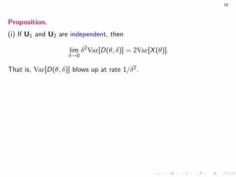
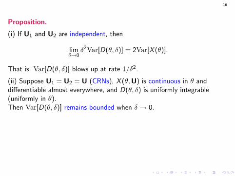
Proposition.
(i) If U1 and U2 are independent, then
limδ→0
δ2Var[D(θ, δ)] = 2Var[X (θ)].
That is, Var[D(θ, δ)] blows up at rate 1/δ2.
(ii) Suppose U1 = U2 = U (CRNs), X (θ,U) is continuous in θ anddifferentiable almost everywhere, and D(θ, δ) is uniformly integrable(uniformly in θ).Then Var[D(θ, δ)] remains bounded when δ → 0.
(iii) Suppose U1 = U2 = U and X (θ,U) is discontinuous in θ, but theprobability that X (·,U) is discontinuous in (θ, θ + δ) converges to 0 asO(δβ) when δ → 0, and X 2+ε(θ) is uniformly integrable for some ε > 0.Then Var[D(θ, δ)] = O(1 + δβ−2−ε), for any ε > 0, when δ → 0.
16
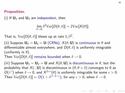
Proposition.
(i) If U1 and U2 are independent, then
limδ→0
δ2Var[D(θ, δ)] = 2Var[X (θ)].
That is, Var[D(θ, δ)] blows up at rate 1/δ2.
(ii) Suppose U1 = U2 = U (CRNs), X (θ,U) is continuous in θ anddifferentiable almost everywhere, and D(θ, δ) is uniformly integrable(uniformly in θ).Then Var[D(θ, δ)] remains bounded when δ → 0.
(iii) Suppose U1 = U2 = U and X (θ,U) is discontinuous in θ, but theprobability that X (·,U) is discontinuous in (θ, θ + δ) converges to 0 asO(δβ) when δ → 0, and X 2+ε(θ) is uniformly integrable for some ε > 0.Then Var[D(θ, δ)] = O(1 + δβ−2−ε), for any ε > 0, when δ → 0.

17
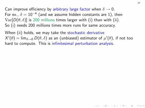
Can improve efficiency by arbitrary large factor when δ → 0.For ex., δ = 10−4 (and we assume hidden constants are 1), thenVar[D(θ, δ)] is 200 millions times larger with (i) than with (ii).So (i) needs 200 millions times more runs for same accuracy.
When (ii) holds, we may take the stochastic derivativeX ′(θ) = limδ→0 D(θ, δ) as an (unbiased) estimator of µ′(θ), if not toohard to compute. This is infinitesimal perturbation analysis.
We may change the definition of X (θ) to make it continuous and benefitfrom (ii). For ex., by replacing some r.v.’s by conditional expectations(conditional Monte Carlo).
For example, if X (θ) counts the customer abandonments, we may replaceeach indicator of abandonment (0 or 1) by the probability of abandonmentgiven the waiting time.
Case (iii) shows that CRNs may provide substantial benefits even if X (θ)is discontinuous.In the call center example, we can prove that (iii) holds with β = 1.
17
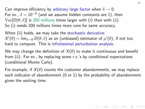
Can improve efficiency by arbitrary large factor when δ → 0.For ex., δ = 10−4 (and we assume hidden constants are 1), thenVar[D(θ, δ)] is 200 millions times larger with (i) than with (ii).So (i) needs 200 millions times more runs for same accuracy.
When (ii) holds, we may take the stochastic derivativeX ′(θ) = limδ→0 D(θ, δ) as an (unbiased) estimator of µ′(θ), if not toohard to compute. This is infinitesimal perturbation analysis.
We may change the definition of X (θ) to make it continuous and benefitfrom (ii). For ex., by replacing some r.v.’s by conditional expectations(conditional Monte Carlo).
For example, if X (θ) counts the customer abandonments, we may replaceeach indicator of abandonment (0 or 1) by the probability of abandonmentgiven the waiting time.
Case (iii) shows that CRNs may provide substantial benefits even if X (θ)is discontinuous.In the call center example, we can prove that (iii) holds with β = 1.
17
Can improve efficiency by arbitrary large factor when δ → 0.For ex., δ = 10−4 (and we assume hidden constants are 1), thenVar[D(θ, δ)] is 200 millions times larger with (i) than with (ii).So (i) needs 200 millions times more runs for same accuracy.
When (ii) holds, we may take the stochastic derivativeX ′(θ) = limδ→0 D(θ, δ) as an (unbiased) estimator of µ′(θ), if not toohard to compute. This is infinitesimal perturbation analysis.
We may change the definition of X (θ) to make it continuous and benefitfrom (ii). For ex., by replacing some r.v.’s by conditional expectations(conditional Monte Carlo).
For example, if X (θ) counts the customer abandonments, we may replaceeach indicator of abandonment (0 or 1) by the probability of abandonmentgiven the waiting time.
Case (iii) shows that CRNs may provide substantial benefits even if X (θ)is discontinuous.In the call center example, we can prove that (iii) holds with β = 1.
18
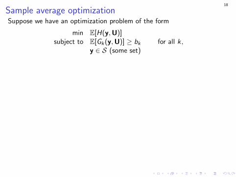
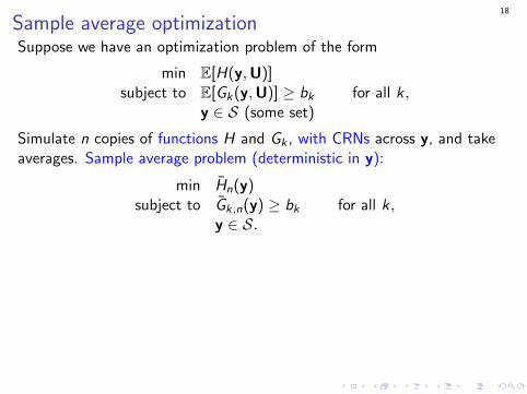
Sample average optimizationSuppose we have an optimization problem of the form
min E[H(y,U)]subject to E[Gk(y,U)] ≥ bk for all k ,
y ∈ S (some set)
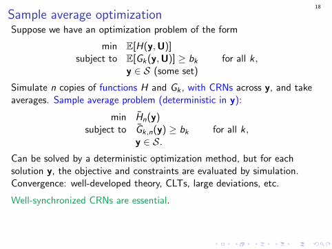
Simulate n copies of functions H and Gk , with CRNs across y, and takeaverages. Sample average problem (deterministic in y):
min Hn(y)subject to Gk,n(y) ≥ bk for all k ,
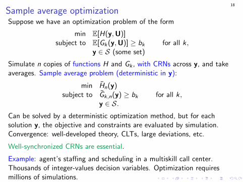
y ∈ S.Can be solved by a deterministic optimization method, but for eachsolution y, the objective and constraints are evaluated by simulation.Convergence: well-developed theory, CLTs, large deviations, etc.
Well-synchronized CRNs are essential.
Example: agent’s staffing and scheduling in a multiskill call center.Thousands of integer-values decision variables. Optimization requiresmillions of simulations.
18
Sample average optimizationSuppose we have an optimization problem of the form
min E[H(y,U)]subject to E[Gk(y,U)] ≥ bk for all k ,
y ∈ S (some set)
Simulate n copies of functions H and Gk , with CRNs across y, and takeaverages. Sample average problem (deterministic in y):
min Hn(y)subject to Gk,n(y) ≥ bk for all k ,
y ∈ S.
Can be solved by a deterministic optimization method, but for eachsolution y, the objective and constraints are evaluated by simulation.Convergence: well-developed theory, CLTs, large deviations, etc.
Well-synchronized CRNs are essential.
Example: agent’s staffing and scheduling in a multiskill call center.Thousands of integer-values decision variables. Optimization requiresmillions of simulations.
18
Sample average optimizationSuppose we have an optimization problem of the form
min E[H(y,U)]subject to E[Gk(y,U)] ≥ bk for all k ,
y ∈ S (some set)
Simulate n copies of functions H and Gk , with CRNs across y, and takeaverages. Sample average problem (deterministic in y):
min Hn(y)subject to Gk,n(y) ≥ bk for all k ,
y ∈ S.Can be solved by a deterministic optimization method, but for eachsolution y, the objective and constraints are evaluated by simulation.Convergence: well-developed theory, CLTs, large deviations, etc.
Well-synchronized CRNs are essential.
Example: agent’s staffing and scheduling in a multiskill call center.Thousands of integer-values decision variables. Optimization requiresmillions of simulations.
18
Sample average optimizationSuppose we have an optimization problem of the form
min E[H(y,U)]subject to E[Gk(y,U)] ≥ bk for all k ,
y ∈ S (some set)
Simulate n copies of functions H and Gk , with CRNs across y, and takeaverages. Sample average problem (deterministic in y):
min Hn(y)subject to Gk,n(y) ≥ bk for all k ,
y ∈ S.Can be solved by a deterministic optimization method, but for eachsolution y, the objective and constraints are evaluated by simulation.Convergence: well-developed theory, CLTs, large deviations, etc.
Well-synchronized CRNs are essential.
Example: agent’s staffing and scheduling in a multiskill call center.Thousands of integer-values decision variables. Optimization requiresmillions of simulations.

19
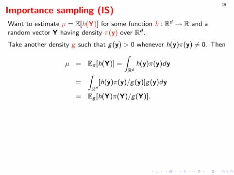
Importance sampling (IS)
Want to estimate µ = E[h(Y)] for some function h : Rd → R and arandom vector Y having density π(y) over Rd .
Take another density g such that g(y) > 0 whenever h(y)π(y) 6= 0. Then
µ = Eπ[h(Y)] =
∫Rd
h(y)π(y)dy
=
∫Rd
[h(y)π(y)/g(y)]g(y)dy
= Eg [h(Y)π(Y)/g(Y)].
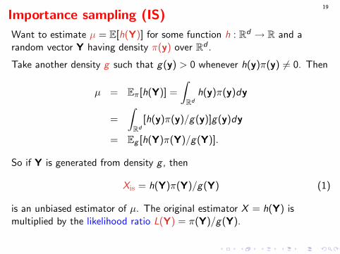
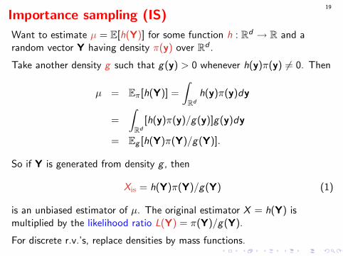
So if Y is generated from density g , then
Xis = h(Y)π(Y)/g(Y) (1)
is an unbiased estimator of µ. The original estimator X = h(Y) ismultiplied by the likelihood ratio L(Y) = π(Y)/g(Y).
For discrete r.v.’s, replace densities by mass functions.
19
Importance sampling (IS)
Want to estimate µ = E[h(Y)] for some function h : Rd → R and arandom vector Y having density π(y) over Rd .
Take another density g such that g(y) > 0 whenever h(y)π(y) 6= 0. Then
µ = Eπ[h(Y)] =
∫Rd
h(y)π(y)dy
=
∫Rd
[h(y)π(y)/g(y)]g(y)dy
= Eg [h(Y)π(Y)/g(Y)].
So if Y is generated from density g , then
Xis = h(Y)π(Y)/g(Y) (1)
is an unbiased estimator of µ. The original estimator X = h(Y) ismultiplied by the likelihood ratio L(Y) = π(Y)/g(Y).
For discrete r.v.’s, replace densities by mass functions.
20
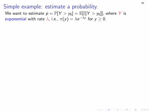
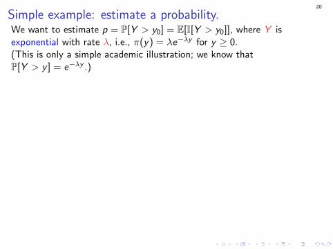
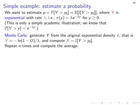
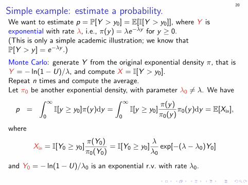
Simple example: estimate a probability.We want to estimate p = P[Y > y0] = E[I[Y > y0]], where Y isexponential with rate λ, i.e., π(y) = λe−λy for y ≥ 0.
(This is only a simple academic illustration; we know thatP[Y > y ] = e−λy .)
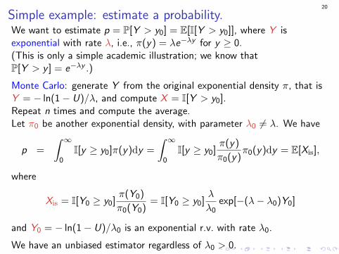
Monte Carlo: generate Y from the original exponential density π, that isY = − ln(1− U)/λ, and compute X = I[Y > y0].Repeat n times and compute the average.Let π0 be another exponential density, with parameter λ0 6= λ. We have
p =
∫ ∞0
I[y ≥ y0]π(y)dy =
∫ ∞0
I[y ≥ y0]π(y)
π0(y)π0(y)dy = E[Xis],
where
Xis = I[Y0 ≥ y0]π(Y0)
π0(Y0)= I[Y0 ≥ y0]
λ
λ0exp[−(λ− λ0)Y0]
and Y0 = − ln(1− U)/λ0 is an exponential r.v. with rate λ0.
We have an unbiased estimator regardless of λ0 > 0.
20
Simple example: estimate a probability.We want to estimate p = P[Y > y0] = E[I[Y > y0]], where Y isexponential with rate λ, i.e., π(y) = λe−λy for y ≥ 0.(This is only a simple academic illustration; we know thatP[Y > y ] = e−λy .)
Monte Carlo: generate Y from the original exponential density π, that isY = − ln(1− U)/λ, and compute X = I[Y > y0].Repeat n times and compute the average.
Let π0 be another exponential density, with parameter λ0 6= λ. We have
p =
∫ ∞0
I[y ≥ y0]π(y)dy =
∫ ∞0
I[y ≥ y0]π(y)
π0(y)π0(y)dy = E[Xis],
where
Xis = I[Y0 ≥ y0]π(Y0)
π0(Y0)= I[Y0 ≥ y0]
λ
λ0exp[−(λ− λ0)Y0]
and Y0 = − ln(1− U)/λ0 is an exponential r.v. with rate λ0.
We have an unbiased estimator regardless of λ0 > 0.
20
Simple example: estimate a probability.We want to estimate p = P[Y > y0] = E[I[Y > y0]], where Y isexponential with rate λ, i.e., π(y) = λe−λy for y ≥ 0.(This is only a simple academic illustration; we know thatP[Y > y ] = e−λy .)
Monte Carlo: generate Y from the original exponential density π, that isY = − ln(1− U)/λ, and compute X = I[Y > y0].Repeat n times and compute the average.Let π0 be another exponential density, with parameter λ0 6= λ. We have
p =
∫ ∞0
I[y ≥ y0]π(y)dy =
∫ ∞0
I[y ≥ y0]π(y)
π0(y)π0(y)dy = E[Xis],
where
Xis = I[Y0 ≥ y0]π(Y0)
π0(Y0)= I[Y0 ≥ y0]
λ
λ0exp[−(λ− λ0)Y0]
and Y0 = − ln(1− U)/λ0 is an exponential r.v. with rate λ0.
We have an unbiased estimator regardless of λ0 > 0.
20
Simple example: estimate a probability.We want to estimate p = P[Y > y0] = E[I[Y > y0]], where Y isexponential with rate λ, i.e., π(y) = λe−λy for y ≥ 0.(This is only a simple academic illustration; we know thatP[Y > y ] = e−λy .)
Monte Carlo: generate Y from the original exponential density π, that isY = − ln(1− U)/λ, and compute X = I[Y > y0].Repeat n times and compute the average.Let π0 be another exponential density, with parameter λ0 6= λ. We have
p =
∫ ∞0
I[y ≥ y0]π(y)dy =
∫ ∞0
I[y ≥ y0]π(y)
π0(y)π0(y)dy = E[Xis],
where
Xis = I[Y0 ≥ y0]π(Y0)
π0(Y0)= I[Y0 ≥ y0]
λ
λ0exp[−(λ− λ0)Y0]
and Y0 = − ln(1− U)/λ0 is an exponential r.v. with rate λ0.
We have an unbiased estimator regardless of λ0 > 0.

21
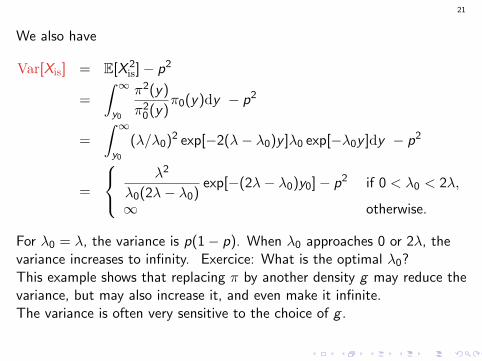
We also have
Var[Xis] = E[X 2is]− p2
=
∫ ∞y0
π2(y)
π20(y)
π0(y)dy − p2
=
∫ ∞y0
(λ/λ0)2 exp[−2(λ− λ0)y ]λ0 exp[−λ0y ]dy − p2
=
λ2
λ0(2λ− λ0)exp[−(2λ− λ0)y0]− p2 if 0 < λ0 < 2λ,
∞ otherwise.
For λ0 = λ, the variance is p(1− p). When λ0 approaches 0 or 2λ, thevariance increases to infinity.
Exercice: What is the optimal λ0?This example shows that replacing π by another density g may reduce thevariance, but may also increase it, and even make it infinite.The variance is often very sensitive to the choice of g .

21
We also have
Var[Xis] = E[X 2is]− p2
=
∫ ∞y0
π2(y)
π20(y)
π0(y)dy − p2
=
∫ ∞y0
(λ/λ0)2 exp[−2(λ− λ0)y ]λ0 exp[−λ0y ]dy − p2
=
λ2
λ0(2λ− λ0)exp[−(2λ− λ0)y0]− p2 if 0 < λ0 < 2λ,
∞ otherwise.
For λ0 = λ, the variance is p(1− p). When λ0 approaches 0 or 2λ, thevariance increases to infinity. Exercice: What is the optimal λ0?
This example shows that replacing π by another density g may reduce thevariance, but may also increase it, and even make it infinite.The variance is often very sensitive to the choice of g .
21
We also have
Var[Xis] = E[X 2is]− p2
=
∫ ∞y0
π2(y)
π20(y)
π0(y)dy − p2
=
∫ ∞y0
(λ/λ0)2 exp[−2(λ− λ0)y ]λ0 exp[−λ0y ]dy − p2
=
λ2
λ0(2λ− λ0)exp[−(2λ− λ0)y0]− p2 if 0 < λ0 < 2λ,
∞ otherwise.
For λ0 = λ, the variance is p(1− p). When λ0 approaches 0 or 2λ, thevariance increases to infinity. Exercice: What is the optimal λ0?This example shows that replacing π by another density g may reduce thevariance, but may also increase it, and even make it infinite.The variance is often very sensitive to the choice of g .
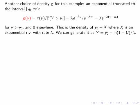
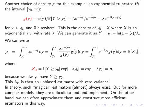
22Another choice of density g for this example: an exponential truncated tothe interval [y0,∞):
g(y) = π(y)/P[Y > y0] = λe−λy/e−λy0 = λe−λ(y−y0)
for y > y0, and 0 elsewhere. This is the density of y0 + X where X is anexponential r.v. with rate λ. We can generate it as Y = y0 − ln(1− U)/λ.
We can write
p =
∫ ∞y0
λe−λydy =
∫ ∞y0
λe−λy
g(y)g(y)dy =
∫ ∞y0
e−λy0g(y)dy = E[Xis],
whereXis = I[Y ≥ y0] exp[−λy0] = exp[−λy0] = p,
because we always have Y ≥ y0.This Xis is then an unbiased estimator with zero variance!In theory, such “magical” estimators (almost) always exist. But for morecomplex models, they are difficult to find and implement. On the otherhand, we can often approximate them and construct more efficientestimators in this way.

22Another choice of density g for this example: an exponential truncated tothe interval [y0,∞):
g(y) = π(y)/P[Y > y0] = λe−λy/e−λy0 = λe−λ(y−y0)
for y > y0, and 0 elsewhere. This is the density of y0 + X where X is anexponential r.v. with rate λ. We can generate it as Y = y0 − ln(1− U)/λ.
We can write
p =
∫ ∞y0
λe−λydy =
∫ ∞y0
λe−λy
g(y)g(y)dy =
∫ ∞y0
e−λy0g(y)dy = E[Xis],
whereXis = I[Y ≥ y0] exp[−λy0] = exp[−λy0] = p,
because we always have Y ≥ y0.This Xis is then an unbiased estimator with zero variance!
In theory, such “magical” estimators (almost) always exist. But for morecomplex models, they are difficult to find and implement. On the otherhand, we can often approximate them and construct more efficientestimators in this way.
22Another choice of density g for this example: an exponential truncated tothe interval [y0,∞):
g(y) = π(y)/P[Y > y0] = λe−λy/e−λy0 = λe−λ(y−y0)
for y > y0, and 0 elsewhere. This is the density of y0 + X where X is anexponential r.v. with rate λ. We can generate it as Y = y0 − ln(1− U)/λ.
We can write
p =
∫ ∞y0
λe−λydy =
∫ ∞y0
λe−λy
g(y)g(y)dy =
∫ ∞y0
e−λy0g(y)dy = E[Xis],
whereXis = I[Y ≥ y0] exp[−λy0] = exp[−λy0] = p,
because we always have Y ≥ y0.This Xis is then an unbiased estimator with zero variance!In theory, such “magical” estimators (almost) always exist. But for morecomplex models, they are difficult to find and implement. On the otherhand, we can often approximate them and construct more efficientestimators in this way.
23
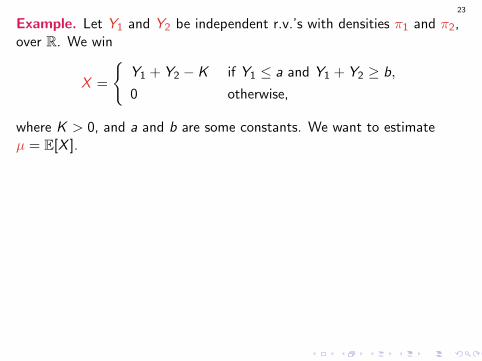
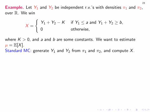
Example. Let Y1 and Y2 be independent r.v.’s with densities π1 and π2,over R. We win
X =
{Y1 + Y2 − K if Y1 ≤ a and Y1 + Y2 ≥ b,
0 otherwise,
where K > 0, and a and b are some constants. We want to estimateµ = E[X ].
Standard MC: generate Y1 and Y2 from π1 and π2, and compute X .
IS strategy: We want to avoid wasting samples in the region where X = 0.Generate Y1 from its density conditional on Y1 < a,then generate Y2 from its density conditional on Y1 + Y2 > b,i.e., truncated to the interval [b − Y1,∞).
The new density of Y1 is
g1(y) = π1(y)/P[Y1 ≤ a] = π1(y)/F1(a)
for y ≤ a, and that of Y2 conditional on Y1 = y1 is
23
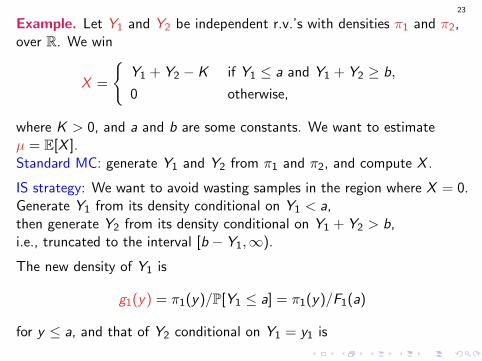
Example. Let Y1 and Y2 be independent r.v.’s with densities π1 and π2,over R. We win
X =
{Y1 + Y2 − K if Y1 ≤ a and Y1 + Y2 ≥ b,
0 otherwise,
where K > 0, and a and b are some constants. We want to estimateµ = E[X ].Standard MC: generate Y1 and Y2 from π1 and π2, and compute X .
IS strategy: We want to avoid wasting samples in the region where X = 0.Generate Y1 from its density conditional on Y1 < a,then generate Y2 from its density conditional on Y1 + Y2 > b,i.e., truncated to the interval [b − Y1,∞).
The new density of Y1 is
g1(y) = π1(y)/P[Y1 ≤ a] = π1(y)/F1(a)
for y ≤ a, and that of Y2 conditional on Y1 = y1 is

23
Example. Let Y1 and Y2 be independent r.v.’s with densities π1 and π2,over R. We win
X =
{Y1 + Y2 − K if Y1 ≤ a and Y1 + Y2 ≥ b,
0 otherwise,
where K > 0, and a and b are some constants. We want to estimateµ = E[X ].Standard MC: generate Y1 and Y2 from π1 and π2, and compute X .
IS strategy: We want to avoid wasting samples in the region where X = 0.Generate Y1 from its density conditional on Y1 < a,then generate Y2 from its density conditional on Y1 + Y2 > b,i.e., truncated to the interval [b − Y1,∞).
The new density of Y1 is
g1(y) = π1(y)/P[Y1 ≤ a] = π1(y)/F1(a)
for y ≤ a, and that of Y2 conditional on Y1 = y1 is
24
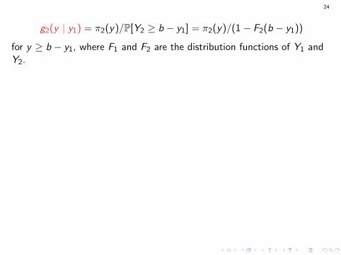
g2(y | y1) = π2(y)/P[Y2 ≥ b − y1] = π2(y)/(1− F2(b − y1))
for y ≥ b − y1, where F1 and F2 are the distribution functions of Y1 andY2.
We have
µ =
∫ ∞−∞
∫ ∞−∞
X π2(y2)π1(y1)dy2dy1
=
∫ a
−∞
∫ ∞b−y1
Xπ2(y2)π1(y1)
g2(y2 | y1)g1(y1)g2(y2 | y1)g1(y1)dy2dy1
=
∫ a
−∞
∫ ∞b−y1
X F1(a) (1− F2(b − y1))g2(y2 | y1)g1(y1)dy2dy1
= E0[Xis],
whereXis = X F1(a) (1− F2(b − Y1))
and E0 denotes the expectation under g1 and g2.
24
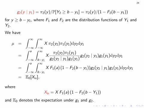
g2(y | y1) = π2(y)/P[Y2 ≥ b − y1] = π2(y)/(1− F2(b − y1))
for y ≥ b − y1, where F1 and F2 are the distribution functions of Y1 andY2.
We have
µ =
∫ ∞−∞
∫ ∞−∞
X π2(y2)π1(y1)dy2dy1
=
∫ a
−∞
∫ ∞b−y1
Xπ2(y2)π1(y1)
g2(y2 | y1)g1(y1)g2(y2 | y1)g1(y1)dy2dy1
=
∫ a
−∞
∫ ∞b−y1
X F1(a) (1− F2(b − y1))g2(y2 | y1)g1(y1)dy2dy1
= E0[Xis],
whereXis = X F1(a) (1− F2(b − Y1))
and E0 denotes the expectation under g1 and g2.
25
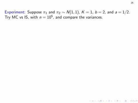
Experiment: Suppose π1 and π2 ∼ N(1, 1), K = 1, b = 2, and a = 1/2.Try MC vs IS, with n = 105, and compare the variances.
We have F1(a) = P[Y1 < a] = P[Y1 − 1 < a− 1] = Φ(a− 1).We put U1 ∼ U(0,Φ(a− 1)) et Y1 = 1 + Φ−1(U1).
We then have1−F2(b−Y1) = P[Y2 > b−Y1] = P[Y2−1 > b−1−Y1] = 1−Φ(b−1−Y1).We put U2 ∼ U(Φ(b − 1− Y1), 1)) and Y2 = 1 + Φ−1(U2).We compute the estimator Xis = XΦ(a− 1)(1− Φ(b − 1− Y1)).The empirical variance S2
n is approximately 40 times smaller with Xis thanwith X .
Estimator µn S2n 95% confidence interval
X 0.0733 0.1188 (0.071, 0.075)Xis 0.0742 0.0027 (0.074, 0.075)

25
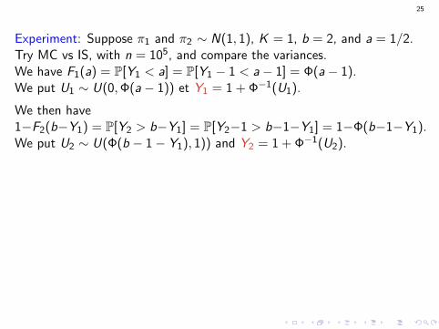
Experiment: Suppose π1 and π2 ∼ N(1, 1), K = 1, b = 2, and a = 1/2.Try MC vs IS, with n = 105, and compare the variances.We have F1(a) = P[Y1 < a] = P[Y1 − 1 < a− 1] = Φ(a− 1).We put U1 ∼ U(0,Φ(a− 1)) et Y1 = 1 + Φ−1(U1).
We then have1−F2(b−Y1) = P[Y2 > b−Y1] = P[Y2−1 > b−1−Y1] = 1−Φ(b−1−Y1).We put U2 ∼ U(Φ(b − 1− Y1), 1)) and Y2 = 1 + Φ−1(U2).We compute the estimator Xis = XΦ(a− 1)(1− Φ(b − 1− Y1)).The empirical variance S2
n is approximately 40 times smaller with Xis thanwith X .
Estimator µn S2n 95% confidence interval
X 0.0733 0.1188 (0.071, 0.075)Xis 0.0742 0.0027 (0.074, 0.075)
25
Experiment: Suppose π1 and π2 ∼ N(1, 1), K = 1, b = 2, and a = 1/2.Try MC vs IS, with n = 105, and compare the variances.We have F1(a) = P[Y1 < a] = P[Y1 − 1 < a− 1] = Φ(a− 1).We put U1 ∼ U(0,Φ(a− 1)) et Y1 = 1 + Φ−1(U1).
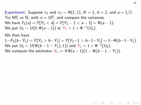
We then have1−F2(b−Y1) = P[Y2 > b−Y1] = P[Y2−1 > b−1−Y1] = 1−Φ(b−1−Y1).We put U2 ∼ U(Φ(b − 1− Y1), 1)) and Y2 = 1 + Φ−1(U2).
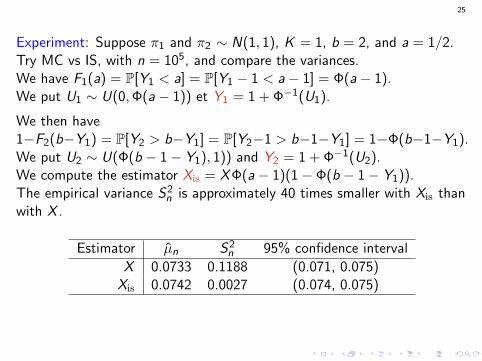
We compute the estimator Xis = XΦ(a− 1)(1− Φ(b − 1− Y1)).The empirical variance S2
n is approximately 40 times smaller with Xis thanwith X .
Estimator µn S2n 95% confidence interval
X 0.0733 0.1188 (0.071, 0.075)Xis 0.0742 0.0027 (0.074, 0.075)
25
Experiment: Suppose π1 and π2 ∼ N(1, 1), K = 1, b = 2, and a = 1/2.Try MC vs IS, with n = 105, and compare the variances.We have F1(a) = P[Y1 < a] = P[Y1 − 1 < a− 1] = Φ(a− 1).We put U1 ∼ U(0,Φ(a− 1)) et Y1 = 1 + Φ−1(U1).
We then have1−F2(b−Y1) = P[Y2 > b−Y1] = P[Y2−1 > b−1−Y1] = 1−Φ(b−1−Y1).We put U2 ∼ U(Φ(b − 1− Y1), 1)) and Y2 = 1 + Φ−1(U2).We compute the estimator Xis = XΦ(a− 1)(1− Φ(b − 1− Y1)).
The empirical variance S2n is approximately 40 times smaller with Xis than
with X .
Estimator µn S2n 95% confidence interval
X 0.0733 0.1188 (0.071, 0.075)Xis 0.0742 0.0027 (0.074, 0.075)
25
Experiment: Suppose π1 and π2 ∼ N(1, 1), K = 1, b = 2, and a = 1/2.Try MC vs IS, with n = 105, and compare the variances.We have F1(a) = P[Y1 < a] = P[Y1 − 1 < a− 1] = Φ(a− 1).We put U1 ∼ U(0,Φ(a− 1)) et Y1 = 1 + Φ−1(U1).
We then have1−F2(b−Y1) = P[Y2 > b−Y1] = P[Y2−1 > b−1−Y1] = 1−Φ(b−1−Y1).We put U2 ∼ U(Φ(b − 1− Y1), 1)) and Y2 = 1 + Φ−1(U2).We compute the estimator Xis = XΦ(a− 1)(1− Φ(b − 1− Y1)).The empirical variance S2
n is approximately 40 times smaller with Xis thanwith X .
Estimator µn S2n 95% confidence interval
X 0.0733 0.1188 (0.071, 0.075)Xis 0.0742 0.0027 (0.074, 0.075)
26
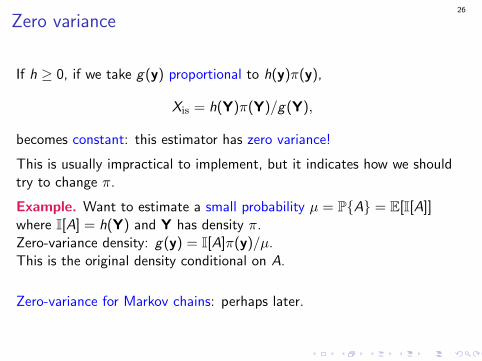
Zero variance
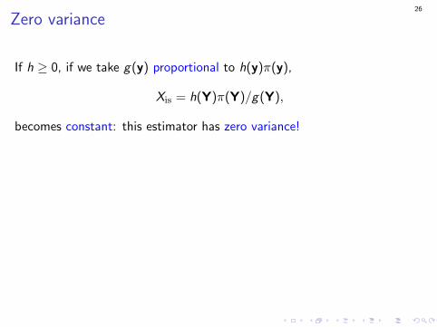
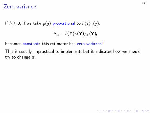
If h ≥ 0, if we take g(y) proportional to h(y)π(y),
Xis = h(Y)π(Y)/g(Y),
becomes constant: this estimator has zero variance!
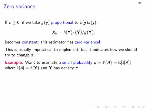
This is usually impractical to implement, but it indicates how we shouldtry to change π.
Example. Want to estimate a small probability µ = P{A} = E[I[A]]where I[A] = h(Y) and Y has density π.Zero-variance density: g(y) = I[A]π(y)/µ.This is the original density conditional on A.
Zero-variance for Markov chains: perhaps later.
26
Zero variance
If h ≥ 0, if we take g(y) proportional to h(y)π(y),
Xis = h(Y)π(Y)/g(Y),
becomes constant: this estimator has zero variance!
This is usually impractical to implement, but it indicates how we shouldtry to change π.
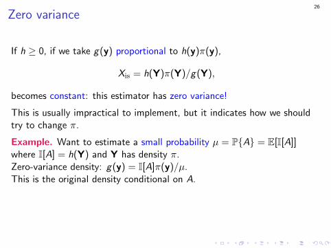
Example. Want to estimate a small probability µ = P{A} = E[I[A]]where I[A] = h(Y) and Y has density π.
Zero-variance density: g(y) = I[A]π(y)/µ.This is the original density conditional on A.
Zero-variance for Markov chains: perhaps later.
26
Zero variance
If h ≥ 0, if we take g(y) proportional to h(y)π(y),
Xis = h(Y)π(Y)/g(Y),
becomes constant: this estimator has zero variance!
This is usually impractical to implement, but it indicates how we shouldtry to change π.
Example. Want to estimate a small probability µ = P{A} = E[I[A]]where I[A] = h(Y) and Y has density π.Zero-variance density: g(y) = I[A]π(y)/µ.This is the original density conditional on A.
Zero-variance for Markov chains: perhaps later.
26
Zero variance
If h ≥ 0, if we take g(y) proportional to h(y)π(y),
Xis = h(Y)π(Y)/g(Y),
becomes constant: this estimator has zero variance!
This is usually impractical to implement, but it indicates how we shouldtry to change π.
Example. Want to estimate a small probability µ = P{A} = E[I[A]]where I[A] = h(Y) and Y has density π.Zero-variance density: g(y) = I[A]π(y)/µ.This is the original density conditional on A.
Zero-variance for Markov chains: perhaps later.
27
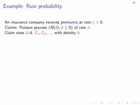
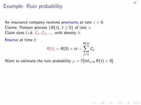
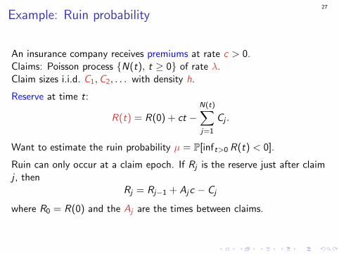
Example: Ruin probability
An insurance company receives premiums at rate c > 0.Claims: Poisson process {N(t), t ≥ 0} of rate λ.Claim sizes i.i.d. C1,C2, . . . with density h.
Reserve at time t:
R(t) = R(0) + ct −N(t)∑j=1
Cj .
Want to estimate the ruin probability µ = P[inft>0 R(t) < 0].
Ruin can only occur at a claim epoch. If Rj is the reserve just after claimj , then
Rj = Rj−1 + Ajc − Cj
where R0 = R(0) and the Aj are the times between claims.
27
Example: Ruin probability
An insurance company receives premiums at rate c > 0.Claims: Poisson process {N(t), t ≥ 0} of rate λ.Claim sizes i.i.d. C1,C2, . . . with density h.
Reserve at time t:
R(t) = R(0) + ct −N(t)∑j=1
Cj .
Want to estimate the ruin probability µ = P[inft>0 R(t) < 0].
Ruin can only occur at a claim epoch. If Rj is the reserve just after claimj , then
Rj = Rj−1 + Ajc − Cj
where R0 = R(0) and the Aj are the times between claims.

28
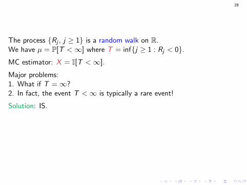
The process {Rj , j ≥ 1} is a random walk on R.We have µ = P[T <∞] where T = inf{j ≥ 1 : Rj < 0}.MC estimator: X = I[T <∞].
Major problems:1. What if T =∞?2. In fact, the event T <∞ is typically a rare event!
Solution: IS.
Change the densities of Aj and Cj so that ruin occurs w.p.1, and multiplyestimator by appropriate likelihood ratio.

28
The process {Rj , j ≥ 1} is a random walk on R.We have µ = P[T <∞] where T = inf{j ≥ 1 : Rj < 0}.MC estimator: X = I[T <∞].
Major problems:1. What if T =∞?2. In fact, the event T <∞ is typically a rare event!
Solution: IS.
Change the densities of Aj and Cj so that ruin occurs w.p.1, and multiplyestimator by appropriate likelihood ratio.

29
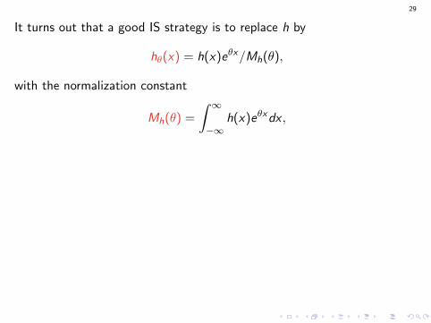
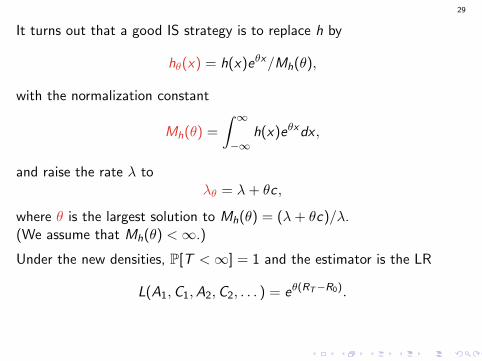
It turns out that a good IS strategy is to replace h by
hθ(x) = h(x)eθx
/Mh(θ),
with the normalization constant
Mh(θ) =
∫ ∞−∞
h(x)eθxdx ,
and raise the rate λ toλθ = λ+ θc ,
where θ is the largest solution to Mh(θ) = (λ+ θc)/λ.(We assume that Mh(θ) <∞.)
Under the new densities, P[T <∞] = 1 and the estimator is the LR
L(A1,C1,A2,C2, . . . ) = eθ(RT−R0).
29
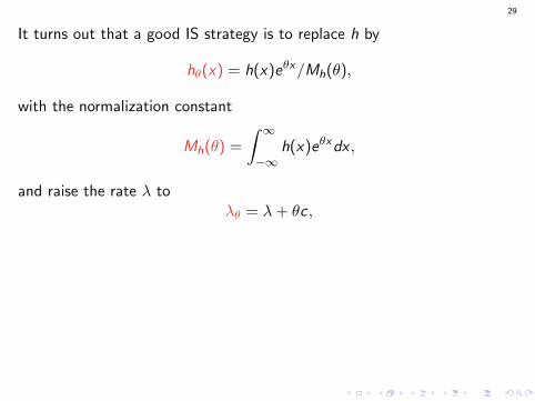
It turns out that a good IS strategy is to replace h by
hθ(x) = h(x)eθx/Mh(θ),
with the normalization constant
Mh(θ) =
∫ ∞−∞
h(x)eθxdx ,
and raise the rate λ toλθ = λ+ θc ,
where θ is the largest solution to Mh(θ) = (λ+ θc)/λ.(We assume that Mh(θ) <∞.)
Under the new densities, P[T <∞] = 1 and the estimator is the LR
L(A1,C1,A2,C2, . . . ) = eθ(RT−R0).
29
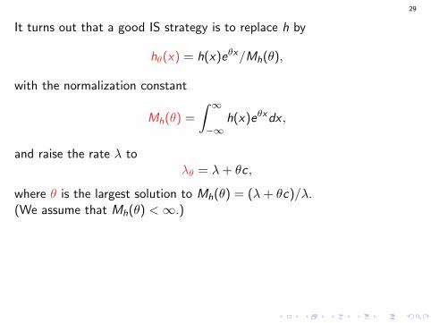
It turns out that a good IS strategy is to replace h by
hθ(x) = h(x)eθx/Mh(θ),
with the normalization constant
Mh(θ) =
∫ ∞−∞
h(x)eθxdx ,
and raise the rate λ toλθ = λ+ θc ,
where θ is the largest solution to Mh(θ) = (λ+ θc)/λ.(We assume that Mh(θ) <∞.)
Under the new densities, P[T <∞] = 1 and the estimator is the LR
L(A1,C1,A2,C2, . . . ) = eθ(RT−R0).
29
It turns out that a good IS strategy is to replace h by
hθ(x) = h(x)eθx/Mh(θ),
with the normalization constant
Mh(θ) =
∫ ∞−∞
h(x)eθxdx ,
and raise the rate λ toλθ = λ+ θc ,
where θ is the largest solution to Mh(θ) = (λ+ θc)/λ.(We assume that Mh(θ) <∞.)
Under the new densities, P[T <∞] = 1 and the estimator is the LR
L(A1,C1,A2,C2, . . . ) = eθ(RT−R0).

30
Numerical illustration
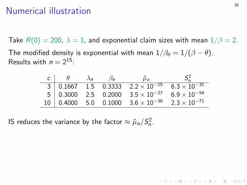
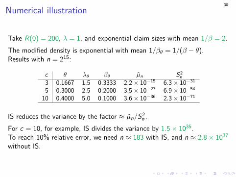
Take R(0) = 200, λ = 1, and exponential claim sizes with mean 1/β = 2.
The modified density is exponential with mean 1/βθ = 1/(β − θ).Results with n = 215:
c θ λθ βθ µn S2n
3 0.1667 1.5 0.3333 2.2× 10⁻¹⁵ 6.3× 10⁻³¹
5 0.3000 2.5 0.2000 3.5× 10⁻²⁷ 6.9× 10−54
10 0.4000 5.0 0.1000 3.6× 10−36 2.3× 10−71
IS reduces the variance by the factor ≈ µn/S2n .
For c = 10, for example, IS divides the variance by 1.5× 1035.To reach 10% relative error, we need n ≈ 183 with IS, and n ≈ 2.8× 1037
without IS.
30
Numerical illustration
Take R(0) = 200, λ = 1, and exponential claim sizes with mean 1/β = 2.
The modified density is exponential with mean 1/βθ = 1/(β − θ).Results with n = 215:
c θ λθ βθ µn S2n
3 0.1667 1.5 0.3333 2.2× 10⁻¹⁵ 6.3× 10⁻³¹
5 0.3000 2.5 0.2000 3.5× 10⁻²⁷ 6.9× 10−54
10 0.4000 5.0 0.1000 3.6× 10−36 2.3× 10−71
IS reduces the variance by the factor ≈ µn/S2n .
For c = 10, for example, IS divides the variance by 1.5× 1035.To reach 10% relative error, we need n ≈ 183 with IS, and n ≈ 2.8× 1037
without IS.
31
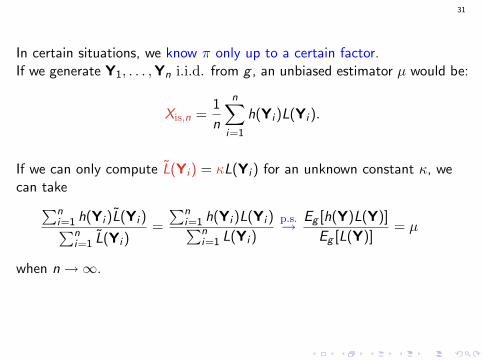
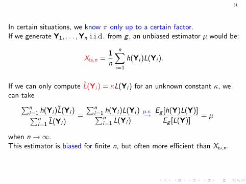
In certain situations, we know π only up to a certain factor.If we generate Y1, . . . ,Yn i.i.d. from g , an unbiased estimator µ would be:
Xis,n =1
n
n∑i=1
h(Yi )L(Yi ).
If we can only compute L(Yi ) = κL(Yi ) for an unknown constant κ, wecan take∑n
i=1 h(Yi )L(Yi )∑ni=1 L(Yi )
=
∑ni=1 h(Yi )L(Yi )∑n
i=1 L(Yi )
p.s.→ Eg [h(Y)L(Y)]
Eg [L(Y)]= µ
when n→∞.
This estimator is biased for finite n, but often more efficient than Xis,n.
31
In certain situations, we know π only up to a certain factor.If we generate Y1, . . . ,Yn i.i.d. from g , an unbiased estimator µ would be:
Xis,n =1
n
n∑i=1
h(Yi )L(Yi ).
If we can only compute L(Yi ) = κL(Yi ) for an unknown constant κ, wecan take∑n
i=1 h(Yi )L(Yi )∑ni=1 L(Yi )
=
∑ni=1 h(Yi )L(Yi )∑n
i=1 L(Yi )
p.s.→ Eg [h(Y)L(Y)]
Eg [L(Y)]= µ
when n→∞.This estimator is biased for finite n, but often more efficient than Xis,n.
32
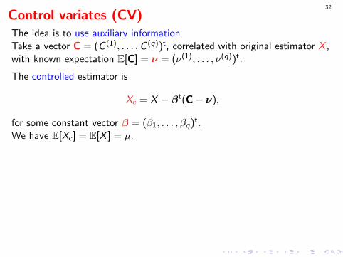
Control variates (CV)The idea is to use auxiliary information.Take a vector C = (C (1), . . . ,C (q))t, correlated with original estimator X ,with known expectation E[C] = ν = (ν(1), . . . , ν(q))t.
The controlled estimator is
Xc = X − βt(C− ν),
for some constant vector β = (β1, . . . , βq)t.We have E[Xc] = E[X ] = µ.
Let ΣC = Cov[C] and ΣCX = (Cov(X ,C (1)), . . . ,Cov(X ,C (q)))t.
Var[Xc] = Var[X ] + βtΣCβ − 2βtΣCX
is minimized by taking
β = β∗ = Σ−1C ΣCX.
32
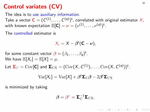
Control variates (CV)The idea is to use auxiliary information.Take a vector C = (C (1), . . . ,C (q))t, correlated with original estimator X ,with known expectation E[C] = ν = (ν(1), . . . , ν(q))t.
The controlled estimator is
Xc = X − βt(C− ν),
for some constant vector β = (β1, . . . , βq)t.We have E[Xc] = E[X ] = µ.
Let ΣC = Cov[C] and ΣCX = (Cov(X ,C (1)), . . . ,Cov(X ,C (q)))t.
Var[Xc] = Var[X ] + βtΣCβ − 2βtΣCX
is minimized by taking
β = β∗ = Σ−1C ΣCX.
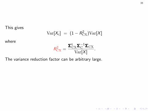
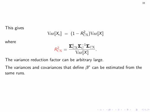
33
This givesVar[Xc] = (1− R2
CX)Var[X ]
where
R2CX =
ΣtCXΣ−1
C ΣCX
Var[X ].
The variance reduction factor can be arbitrary large.
The variances and covariances that define β∗ can be estimated from thesame runs.
33
This givesVar[Xc] = (1− R2
CX)Var[X ]
where
R2CX =
ΣtCXΣ−1
C ΣCX
Var[X ].
The variance reduction factor can be arbitrary large.
The variances and covariances that define β∗ can be estimated from thesame runs.
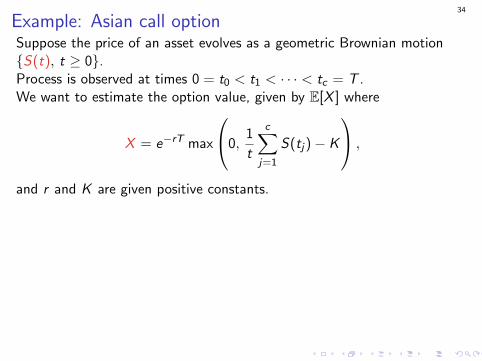
34
Example: Asian call optionSuppose the price of an asset evolves as a geometric Brownian motion{S(t), t ≥ 0}.Process is observed at times 0 = t0 < t1 < · · · < tc = T .We want to estimate the option value, given by E[X ] where
X = e−rT max
0,1
t
c∑j=1
S(tj)− K
,
and r and K are given positive constants.
If we replace the arithmetic average by a geometric average, we obtain
C = e−rT max
0,c∏
j=1
(S(tj))1/c − K
,
whose expectation ν = E[C ] has a closed-form formula.
By using C as a CV for X , we can obtain huge variance reductions, byfactors of up to a million in some examples.
34
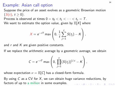
Example: Asian call optionSuppose the price of an asset evolves as a geometric Brownian motion{S(t), t ≥ 0}.Process is observed at times 0 = t0 < t1 < · · · < tc = T .We want to estimate the option value, given by E[X ] where
X = e−rT max
0,1
t
c∑j=1
S(tj)− K
,
and r and K are given positive constants.
If we replace the arithmetic average by a geometric average, we obtain
C = e−rT max
0,c∏
j=1
(S(tj))1/c − K
,
whose expectation ν = E[C ] has a closed-form formula.
By using C as a CV for X , we can obtain huge variance reductions, byfactors of up to a million in some examples.
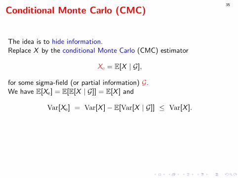
35
Conditional Monte Carlo (CMC)
The idea is to hide information.Replace X by the conditional Monte Carlo (CMC) estimator
Xe = E[X | G],
for some sigma-field (or partial information) G.We have E[Xe] = E[E[X | G]] = E[X ] and
Var[Xe] = Var[X ]− E[Var[X | G]] ≤ Var[X ].
Choice of G is a matter of compromise. The less information it contains,the more the variance is reduced, but the more difficult is the computationof Xe.

36
CMC rarely brings a large gain just by itself.
But it can be a very powerful tool to make the estimator continuous, sothat IPA can be applied.
Particularly useful when the original estimator is integer-valued (e.g., anindicator). That can really boost the efficiency of CRNs for derivativeestimation (or small differences).Example. In the call center, suppose we want to estimate the expectednumber of abandonments in a day, and its derivative w.r.t. the meanservice time θ. The standard estimator X (θ) is integer-valued, anddiscontinuous in θ for fixed U.
Idea: erase all traces of abandoning calls, and compute their expectednumber, conditional on the information that remains.Multiply the arrival rate at t by the probability that a call arriving at twould abandon, and integrate w.r.t. t.Other examples: barrier options, number of waits > `, ...

36
CMC rarely brings a large gain just by itself.
But it can be a very powerful tool to make the estimator continuous, sothat IPA can be applied.
Particularly useful when the original estimator is integer-valued (e.g., anindicator). That can really boost the efficiency of CRNs for derivativeestimation (or small differences).
Example. In the call center, suppose we want to estimate the expectednumber of abandonments in a day, and its derivative w.r.t. the meanservice time θ. The standard estimator X (θ) is integer-valued, anddiscontinuous in θ for fixed U.
Idea: erase all traces of abandoning calls, and compute their expectednumber, conditional on the information that remains.Multiply the arrival rate at t by the probability that a call arriving at twould abandon, and integrate w.r.t. t.Other examples: barrier options, number of waits > `, ...

36
CMC rarely brings a large gain just by itself.
But it can be a very powerful tool to make the estimator continuous, sothat IPA can be applied.
Particularly useful when the original estimator is integer-valued (e.g., anindicator). That can really boost the efficiency of CRNs for derivativeestimation (or small differences).Example. In the call center, suppose we want to estimate the expectednumber of abandonments in a day, and its derivative w.r.t. the meanservice time θ.
The standard estimator X (θ) is integer-valued, anddiscontinuous in θ for fixed U.
Idea: erase all traces of abandoning calls, and compute their expectednumber, conditional on the information that remains.Multiply the arrival rate at t by the probability that a call arriving at twould abandon, and integrate w.r.t. t.Other examples: barrier options, number of waits > `, ...
36
CMC rarely brings a large gain just by itself.
But it can be a very powerful tool to make the estimator continuous, sothat IPA can be applied.
Particularly useful when the original estimator is integer-valued (e.g., anindicator). That can really boost the efficiency of CRNs for derivativeestimation (or small differences).Example. In the call center, suppose we want to estimate the expectednumber of abandonments in a day, and its derivative w.r.t. the meanservice time θ. The standard estimator X (θ) is integer-valued, anddiscontinuous in θ for fixed U.
Idea: erase all traces of abandoning calls, and compute their expectednumber, conditional on the information that remains.Multiply the arrival rate at t by the probability that a call arriving at twould abandon, and integrate w.r.t. t.Other examples: barrier options, number of waits > `, ...

36
CMC rarely brings a large gain just by itself.
But it can be a very powerful tool to make the estimator continuous, sothat IPA can be applied.
Particularly useful when the original estimator is integer-valued (e.g., anindicator). That can really boost the efficiency of CRNs for derivativeestimation (or small differences).Example. In the call center, suppose we want to estimate the expectednumber of abandonments in a day, and its derivative w.r.t. the meanservice time θ. The standard estimator X (θ) is integer-valued, anddiscontinuous in θ for fixed U.
Idea: erase all traces of abandoning calls, and compute their expectednumber, conditional on the information that remains.Multiply the arrival rate at t by the probability that a call arriving at twould abandon, and integrate w.r.t. t.
Other examples: barrier options, number of waits > `, ...
36
CMC rarely brings a large gain just by itself.
But it can be a very powerful tool to make the estimator continuous, sothat IPA can be applied.
Particularly useful when the original estimator is integer-valued (e.g., anindicator). That can really boost the efficiency of CRNs for derivativeestimation (or small differences).Example. In the call center, suppose we want to estimate the expectednumber of abandonments in a day, and its derivative w.r.t. the meanservice time θ. The standard estimator X (θ) is integer-valued, anddiscontinuous in θ for fixed U.
Idea: erase all traces of abandoning calls, and compute their expectednumber, conditional on the information that remains.Multiply the arrival rate at t by the probability that a call arriving at twould abandon, and integrate w.r.t. t.Other examples: barrier options, number of waits > `, ...
37
Generalized AV and randomized quasi-Monte Carlo(RQMC)Estimate µ by average of X (1), . . . ,X (k), each with same distribution as X :
Xa =1
k
k∑i=1
X (i).
Its variance is
Var[Xa] =1
k2
k∑j=1
k∑`=1
Cov[X (j),X (`)]
=Var[X ]
k+
2
k2
∑j<`
Cov[X (j),X (`)].
We want to make the last sum as negative as possible.
Special cases: antithetic variates (k = 2), Latin hypercube sampling,randomized quasi-Monte Carlo (RQMC).
38
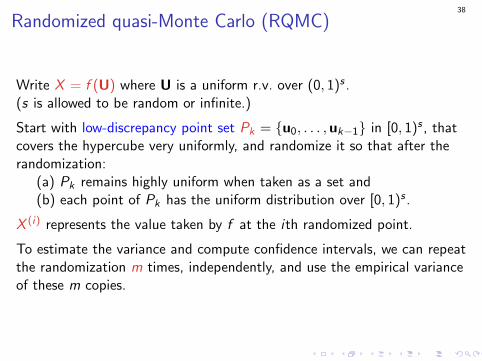
Randomized quasi-Monte Carlo (RQMC)
Write X = f (U) where U is a uniform r.v. over (0, 1)s .(s is allowed to be random or infinite.)
Start with low-discrepancy point set Pk = {u0, . . . ,uk−1} in [0, 1)s , thatcovers the hypercube very uniformly, and randomize it so that after therandomization:
(a) Pk remains highly uniform when taken as a set and(b) each point of Pk has the uniform distribution over [0, 1)s .
X (i) represents the value taken by f at the ith randomized point.
To estimate the variance and compute confidence intervals, we can repeatthe randomization m times, independently, and use the empirical varianceof these m copies.
38
Randomized quasi-Monte Carlo (RQMC)
Write X = f (U) where U is a uniform r.v. over (0, 1)s .(s is allowed to be random or infinite.)
Start with low-discrepancy point set Pk = {u0, . . . ,uk−1} in [0, 1)s , thatcovers the hypercube very uniformly, and randomize it so that after therandomization:
(a) Pk remains highly uniform when taken as a set and(b) each point of Pk has the uniform distribution over [0, 1)s .
X (i) represents the value taken by f at the ith randomized point.
To estimate the variance and compute confidence intervals, we can repeatthe randomization m times, independently, and use the empirical varianceof these m copies.

39
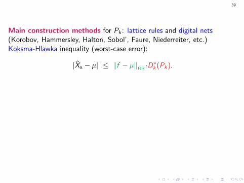
Main construction methods for Pk : lattice rules and digital nets(Korobov, Hammersley, Halton, Sobol’, Faure, Niederreiter, etc.)
Koksma-Hlawka inequality (worst-case error):
|Xa − µ| ≤ ‖f − µ‖HK ·D∗k (Pk).
With MC: D∗k (Pk) ≈ O(k−1/2).With best QMC sequences: D∗k (Pk) = O(k−1(ln k)s).Can be very effective in practice, provided that the integrand f has (or canbe modified to have) low effective dimension.
This means that f can be well approximated by a sum of low-dimensionalfunctions. Then, if the point set is constructed to have high uniformity(low discrepancy) for its corresponding projections, we are in business.
39
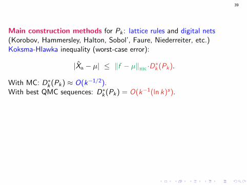
Main construction methods for Pk : lattice rules and digital nets(Korobov, Hammersley, Halton, Sobol’, Faure, Niederreiter, etc.)Koksma-Hlawka inequality (worst-case error):
|Xa − µ| ≤ ‖f − µ‖HK ·D∗k (Pk).
With MC: D∗k (Pk) ≈ O(k−1/2).With best QMC sequences: D∗k (Pk) = O(k−1(ln k)s).Can be very effective in practice, provided that the integrand f has (or canbe modified to have) low effective dimension.
This means that f can be well approximated by a sum of low-dimensionalfunctions. Then, if the point set is constructed to have high uniformity(low discrepancy) for its corresponding projections, we are in business.
39
Main construction methods for Pk : lattice rules and digital nets(Korobov, Hammersley, Halton, Sobol’, Faure, Niederreiter, etc.)Koksma-Hlawka inequality (worst-case error):
|Xa − µ| ≤ ‖f − µ‖HK ·D∗k (Pk).
With MC: D∗k (Pk) ≈ O(k−1/2).With best QMC sequences: D∗k (Pk) = O(k−1(ln k)s).
Can be very effective in practice, provided that the integrand f has (or canbe modified to have) low effective dimension.
This means that f can be well approximated by a sum of low-dimensionalfunctions. Then, if the point set is constructed to have high uniformity(low discrepancy) for its corresponding projections, we are in business.

39
Main construction methods for Pk : lattice rules and digital nets(Korobov, Hammersley, Halton, Sobol’, Faure, Niederreiter, etc.)Koksma-Hlawka inequality (worst-case error):
|Xa − µ| ≤ ‖f − µ‖HK ·D∗k (Pk).
With MC: D∗k (Pk) ≈ O(k−1/2).With best QMC sequences: D∗k (Pk) = O(k−1(ln k)s).Can be very effective in practice, provided that the integrand f has (or canbe modified to have) low effective dimension.
This means that f can be well approximated by a sum of low-dimensionalfunctions. Then, if the point set is constructed to have high uniformity(low discrepancy) for its corresponding projections, we are in business.
40
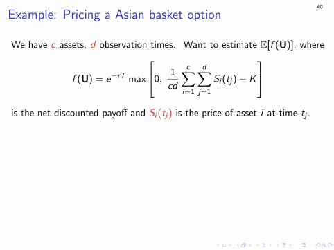
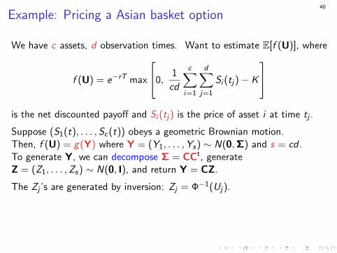
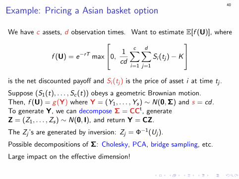
Example: Pricing a Asian basket option
We have c assets, d observation times. Want to estimate E[f (U)], where
f (U) = e−rT max
0,1
cd
c∑i=1
d∑j=1
Si (tj)− K
is the net discounted payoff and Si (tj) is the price of asset i at time tj .
Suppose (S1(t), . . . ,Sc(t)) obeys a geometric Brownian motion.Then, f (U) = g(Y) where Y = (Y1, . . . ,Ys) ∼ N(0,Σ) and s = cd .To generate Y, we can decompose Σ = CCt, generateZ = (Z1, . . . ,Zs) ∼ N(0, I), and return Y = CZ.
The Zj ’s are generated by inversion: Zj = Φ−1(Uj).
Possible decompositions of Σ: Cholesky, PCA, bridge sampling, etc.
Large impact on the effective dimension!

40
Example: Pricing a Asian basket option
We have c assets, d observation times. Want to estimate E[f (U)], where
f (U) = e−rT max
0,1
cd
c∑i=1
d∑j=1
Si (tj)− K
is the net discounted payoff and Si (tj) is the price of asset i at time tj .
Suppose (S1(t), . . . ,Sc(t)) obeys a geometric Brownian motion.Then, f (U) = g(Y) where Y = (Y1, . . . ,Ys) ∼ N(0,Σ) and s = cd .
To generate Y, we can decompose Σ = CCt, generateZ = (Z1, . . . ,Zs) ∼ N(0, I), and return Y = CZ.
The Zj ’s are generated by inversion: Zj = Φ−1(Uj).
Possible decompositions of Σ: Cholesky, PCA, bridge sampling, etc.
Large impact on the effective dimension!
40
Example: Pricing a Asian basket option
We have c assets, d observation times. Want to estimate E[f (U)], where
f (U) = e−rT max
0,1
cd
c∑i=1
d∑j=1
Si (tj)− K
is the net discounted payoff and Si (tj) is the price of asset i at time tj .
Suppose (S1(t), . . . ,Sc(t)) obeys a geometric Brownian motion.Then, f (U) = g(Y) where Y = (Y1, . . . ,Ys) ∼ N(0,Σ) and s = cd .To generate Y, we can decompose Σ = CCt, generateZ = (Z1, . . . ,Zs) ∼ N(0, I), and return Y = CZ.
The Zj ’s are generated by inversion: Zj = Φ−1(Uj).
Possible decompositions of Σ: Cholesky, PCA, bridge sampling, etc.
Large impact on the effective dimension!
41
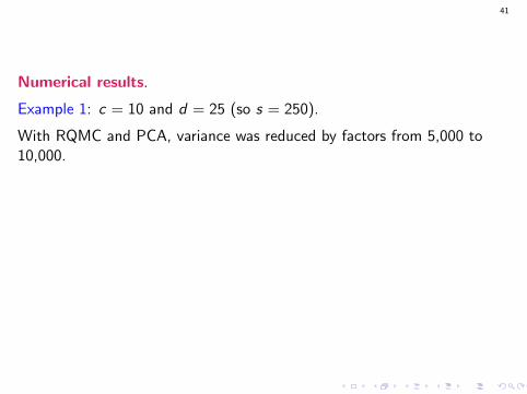
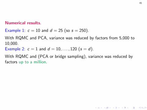
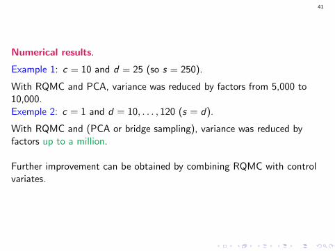
Numerical results.
Example 1: c = 10 and d = 25 (so s = 250).
With RQMC and PCA, variance was reduced by factors from 5,000 to10,000.
Exemple 2: c = 1 and d = 10, . . . , 120 (s = d).
With RQMC and (PCA or bridge sampling), variance was reduced byfactors up to a million.
Further improvement can be obtained by combining RQMC with controlvariates.
41
Numerical results.
Example 1: c = 10 and d = 25 (so s = 250).
With RQMC and PCA, variance was reduced by factors from 5,000 to10,000.Exemple 2: c = 1 and d = 10, . . . , 120 (s = d).
With RQMC and (PCA or bridge sampling), variance was reduced byfactors up to a million.
Further improvement can be obtained by combining RQMC with controlvariates.

42
Array-RQMC: new RQMC method developed specially for the simulationof Markov chains over several steps (L’Ecuyer, Lecot, Tuffin, OperationsResearch 2008).
43
Conclusion
I Cleverly modified estimators can often bring huge statistical efficiencyimprovements in simulations.
I In certain settings (e.g., rare events, sample-average optimization,gradient estimation), they are essential.
I We still have a lot to learn in that area.Many opportunities are waiting to be exploited.