Graduate Theses and Dissertations Iowa State University Capstones, Theses andDissertations

2012

Variation in plant defense traits and populationgenetics within a Sonoran Desert cotton endemic,Gossypium davidsonii and boll weevil,Anthonomus grandisAdam KuesterIowa State University

Follow this and additional works at: https://lib.dr.iastate.edu/etd

Part of the Entomology Commons, Evolution Commons, and the Plant Sciences Commons

This Dissertation is brought to you for free and open access by the Iowa State University Capstones, Theses and Dissertations at Iowa State UniversityDigital Repository. It has been accepted for inclusion in Graduate Theses and Dissertations by an authorized administrator of Iowa State UniversityDigital Repository. For more information, please contact digirep@iastate.edu.

Recommended CitationKuester, Adam, "Variation in plant defense traits and population genetics within a Sonoran Desert cotton endemic, Gossypiumdavidsonii and boll weevil, Anthonomus grandis" (2012). Graduate Theses and Dissertations. 12371.https://lib.dr.iastate.edu/etd/12371

Variation in plant defense traits and population genetics within a Sonoran Desert

cotton endemic, Gossypium davidsonii and boll weevil, Anthonomus grandis

by

Adam P. Kuester

A dissertation submitted to the graduate faculty

in partial fulfillment of the requirements for the degree of

DOCTOR OF PHILOSOPHY

Major: Genetics

Program of Study Committee:

John Nason, Major Professor

Thomas Sappington

Jonathan Wendel

Fredric Janzen

Matthew O’Neal

Iowa State University

Ames, Iowa

2012

ii

TABLE OF CONTENTS

CHAPTER1. General Introduction

CHAPTER 2. Abiotic and biotic stress affects on defense trait

phenotypes in a wild cotton species, Gossypium davidsonii

CHAPTER 3. Response of herbivory to defense traits, geographic and

genetic structure within a Sonoran Desert wild cotton species,

Gossypium davidsonii

CHAPTER 4. Comparison of quantitative defense traits and genetics

in determining evolution of defense syndromes in a wild Sonoran

Desert cotton endemic, Gossypium davidsonii

CHAPTER 5. Covariation in the geographic genetic structures of a

wild cotton, Gossypium davidsonii, and associated boll weevil,

Anthonomus grandis

CHAPTER 6. Population structure and genetic diversity of the boll

weevil, Anthonomus grandis, in North America

CHAPTER 7. General Conclusions

APPENDIX. DNA Sequencing

1

12

54

90

137

182

234

238

1

CHAPTER 1. General Introduction

Introduction

Understanding the evolutionary mechanisms behind plant defense can be very

important in determining how plant populations have evolved to cope with associated insect

herbivores. Not surprisingly, vascular plants have developed complex chemical and physical

strategies to defend themselves against them. While such strategies can be effective at

reducing herbivory, investment in defenses often comes as a tradeoff with other processes (as

reviewed in Herms and Mattson, 1992; Simms, 1992; Hakulinen et al., 1995; Haukioja et al.,

1998; Haugen et al., 2008; Moreno et al., 2009).

Defense trait variation may, in fact, create quite different responses by associated

insect herbivores. For instance, specialist herbivores that rely on Gossypium plants for

development are attracted by particular colors of cotton leaves and high levels of plant

terpenoids (Lincoln and Boyer 1975, Hedin and McCarty 1995), whereas generalist folivores

tend to tolerate lower levels of plant toxins and varying degrees of leaf pubescence

depending on feeding habit (Lincoln and Boyer 1975; Stipanovic et al. 2008). Additional

levels of plant defense through response of tertiary trophic predators can drastically alter

herbivore communities.

The initial reason for host preference across an insect herbivore’s species range is

frequently related to host availability and distribution within a particular location, but also

can stem from variation in host plant phenotypes. An insect may have higher reproductive

output or faster growth rates on plants that exhibit particular characters, leading to greater

selection on plant populations against less fit defense syndromes.

2

Recent studies suggest that patterns of gene flow within interacting species can be an

important determinant of their coevolutionary dynamics (Thompson and Burdon, 1992;

Nuismer et al., 1999; Forde and Thompson, 2004; Hoeksema and Forde, 2008; Vogwill et al.,

2008; Gandon and Nuismer, 2009). Indeed, that outcomes of inter-species interactions are

influenced by the level and spatial patterning of gene flow between populations of both

species is a central component of the geographic mosaic theory of coevolution (Thompson,

2005; Gomulkiewicz et al. 2007). In plant-insect systems, the nature of the inter-specific

interaction can influence the amount and geographical symmetry of gene flow between

populations of both organisms. In particular, interactions in which an insect directly affects

plant dispersal through pollination and seed distribution are more likely to contribute to the

geographical symmetry of gene flow between the two species.

Regardless of this symmetry, very low rates of gene flow within taxa tend to limit

local adaptive genetic variation and the rates of coevolutionary change, while very high

levels of gene flow can cause local maladaptation by limiting the effectiveness of reciprocal

selection. Theoretical studies indicate, however, that with greater symmetry of gene flow

between symbionts, localities with stronger reciprocal selection tend to dominate global

coevolutionary patterns (Nuismer et al. 1999; Gomulkiewicz et al. 2000).

In addition to host association and gene flow within species of insect herbivores,

inter-species dynamics is also of interest by illuminating geographical effects and host race

associations through genetic structuring of insect herbivores that have broader host diets.

Insect species that are hosted by one to several species of plants may be genetically

structured simply as a result of isolation by distance or by prefence of a particular plant host.

3

Research Rationale:

Recognizing the mechanisms and patterns of evolution of natural plant defenses not

only allows us to understand how to reasonably control host associated pest populations, but

also to direct better-suited breeding and selection programs for traits associated with

tolerance or resistance to otherwise uncontrollable pests (Gould 1988; Cortesero et al. 1999;

Rausher 2001; Thrall et al. 2011). Though this thesis work focuses on Gossypium davidsonii,

similar defense traits and responses to herbivory can be seen in many of the New World

cotton species (Rudgers et al. 2004). Understanding how plants respond to herbivory in

natural systems should provide us with insights into variation in traits that may provide

resistance within agronomic settings. Additionally, population genetic studies of associated

pest insects have identified approaches that best control associated insect herbivore

populations (Porreta et al., 2007).

Study System

Gossypium davidsonii is a wild diploid cotton species that is endemic to the Sonoran

Desert of northwestern Mexico, found in the subsection Integrifolia within the genus

Gossypium (Family Malvaceae). It is commonly characterized as a branched shrub between

1-3 meters in height, with lobed to entire cordate leaves. The species is found from sea level

to 400 m elevation with primary range within the lower Cape region of the Baja Peninsula.

Habitat ranges from open to thorn-scrub vegetation in disturbed or rocky areas.

Like most cotton species, G. davidsonii exhibits several characteristic defense traits.

Though variation in nectary presence has been previously noted (Phillips and Clements,

1967), we detect no biological reason for selection on nectaries, as no myrmechophyllic

4

interaction with associated ants has been observed within populations of the species (pers.

obs.). Another common defense trait among cotton species is presence of pigmented glands

on aerial plant parts in which gossypol and related terpene aldehyde anti-herbivore defense

compounds are stored. Pigment gland densities on fruit capsules have been noted to vary

among populations from 250-300 glands per capsule and foliar quantities of glands make up

between 1.8 – 2.0 % of leaf dry weight within the species (Phillips and Clements, 1967).

Gossypium davidsonii expresses higher concentrations of gossypol in seed and leaf tissue

than any other species (Khan, 1999; Stipanovic et al., 2005). Gossypol concentration varies

up to 6-fold among populations from Baja California’s Cape Region in both seed and leaf

tissues, despite sample sites being located <150 km apart (Stipanovic et al., 2005). Little

attention has been devoted, however, to understanding why G. davidsonii (or any other

cotton) produces large amounts of this compound, or why levels of gossypol expression vary

so extensively among populations.

Wild New World cotton species have been well studied in terms of their variation for

desired traits, such as fiber production (Mei et al. 2004; Park et al., 2005), chemical defenses

(Stipanovic, 1986; Stipanovic et al., 2003), and oil content (Gotmare et al., 2004). Other

aspects of their natural history, however, are not well understood. On the one hand, many of

the New World species have large, showy flowers, suggesting that they are attractive for

pollinators, have out-crossing mating systems, and experience appreciable gene flow. On the

other hand, studies of wild cottons have found low levels of genetic variability at putatively

neutral genetic marker loci, including G. davidsonii (AFLPs: Alvarez and Wendel, 2006;

allozymes: Wendel and Percival, 1990), suggesting that cottons have intrinsically high levels

5

of inbreeding via selfing and restricted gene flow. Studies addressing this conflict have yet to

be conducted in populations of any wild cotton species.

The boll weevil, Anthonomus grandis, has been studied on domesticated cotton, both

in the southeastern United States and in Mexico, but is also found on many wild cotton host

species, including G. davidsonii (Cross, 1973). The boll weevil undergoes complete

development within flower buds or fruits on cotton plants (Burke et al., 1986). Population

genetic studies of A. grandis populations on cotton cultivars have shown patterns of isolation

by distance and high levels of recent gene flow among boll weevil populations (Kim and

Sappington, 2004; Kim and Sappington, 2006).

The boll weevil, Anthonomus grandis grandis Boheman (Curculionidae), has been a

major pest of commercial cotton in the United States for more than a century and is still of

concern in southern Texas and parts of northern Mexico and Central and South America

(Burke et al., 1986; Scataglini et al., 2005). First identified in 1843 by the Swedish

entomologist Karl Boheman from samples collected in Veracruz, Mexico, the insect crossed

the Rio Grande in 1892 and quickly moved through the cotton belt of the southeastern United

States, becoming the most expensive agricultural insect pest in U.S. history (Burke et al.,

1986; Allen, 2008).

Though the boll weevil has been identified on several cotton hosts (Cross et al. 1975),

and studied thoroughly for distinguishing morphological characteristics among economically

and ecologically important groups (henceforth referred to as forms) of boll weevil, few

genetic studies have established any resolution distinguishing geographic, ecological, or host-

associated forms (Roehrdanz, 2001; Roehrdanz et al., 2010).

6

Thesis Organization

We are interested in understanding the exceptionally large marked variation in

defense phenotypes observed among and within populations of Gossypium davidsonii. We

will determine the extent to which defense trait variation is a response to environmental

stresses. In particular, we determine the degree to which mechanical damage (a simulated

form of herbivory) and extreme water and nutrient availability affect plant defense within the

species. From assessment of environmental effects on foliar trichome density, lysigenous

cavity density and gossypol concentration will elucidate the extent of trait plasticity or

whether traits are based on genetic differentiation among populations, or a combination of

environment and genetic effects.

Variation in defense traits may influence the interaction with associated insect

herbivores. We will extend the analysis of defense trait phenotypes, genetic relatedness, and

spatial structuring of populations of G. davidsonii on fitness responses and seed and leaf

damage. We also assess spatial autocorrelation of genetic and phenotypic relatedness, within

four populations of the species reflecting the species’ range.

Variation in plant defense, on the other hand, may be attributable to a response of

natural selection or stochastic processes of genetic drift and migration. We determine

whether observed variation in defense phenotypes is in response to linear (directional)

selection or whether observed traits are a product of merely stochastic events such as genetic

drift and migration, which will be assessed in a PST-FST study.

Having observed genetic structuring within G. davidsonii populations within the

southern cape region of the Baja Peninsula, we determine whether ancestral and

contemporary gene flow within A. grandis-associated populations of G. davidsonii and A.

7

grandis are symmetrical. We assess gene flow measurements by using traditional measures

of FST, as well as analytical methods of contemporary (Bayesian methods: structure,

Likelihood method: GeneClass) and ancestral (Population Graphs) gene flow.

Lastly, we assess the population genetic structure of the boll weevil in North America

on cultivated and wild cotton hosts. We reassess classification of boll weevil groups and

determine a most parsimonious classification given the genetic data.

Contributions of Authors

For all work described within this dissertation, my contributions were as primary

researcher and author, though each listed co-author in my research chapters has had an

essential role in the successful completion of the described dissertation work. In Chapters 2

through 4, Dr. John Nason contributed substantially to the intellectual development of the

manuscripts. Chapter 5 benefited from intellectual criticism from Dr. Thomas Sappington, Dr.

Kyung Seok Kim and Dr. John Nason. Genotyping was also performed under the direction of

K.S. Kim for Chapter 5. Chapter 6 profited from input from many boll weevil biologists, but

in particular from co-authors, Dr. Robert Jones, Dr. Thomas Sappinton, Dr. Kyung Seok Kim,

Dr. Norman Barr, Dr. Richard Roehrdanz and Dr. John Nason. Some sequence data used in

Chapter 6 were obtained from N. Barr and P. Senechal (described within Chapter 6). Field

collections of boll weevil specimen were also made in collaboration with R. Jones, R.

Roehrdanz and N. Barr.

8

Literature Cited

Allen CT (2008) Boll Weevil Eradication: an Areawide Pest Management Effort. In:

Areawide Pest Management Theory and Implementation (ed. Koul O, G. Cuperus, N. Elliot),

pp. 467-559. CAB International, Cambridge, Ma.

Alvarez I and JF Wendel (2006) Cryptic Interspecific Introgression and Genetic

Differentiation Within Gossypium aridum (Malvaceae) and Its Relatives. Evolution 60, 505-

517.

Burke HR, WE Clark, JR Cate, PA Fryxell (1986) Origin and Dispersal of the Boll Weevil.

Bulletin Entomological Society America 32, 228-238.

Cortesero A, JO Stapel, WJ Lewis (1999) Understanding and Manipulating Plant Attributes

to Enhance Biological Control. Biological Control 17, 35-49.

Cross WH (1973) Biology, Control, and Eradication of the Boll Weevil. Annual Review of

Entomology 18, 17-46.

Cross WH, MJ Lukefahr, PA Fryxell, HR Burke (1975) Host plants of boll-weevil.

Environmental Entomology 4, 19-26.

Forde SE, JN Thompson, BJM Bohannan (2004) Adaptation varies through space and time in

a coevolving host-parasitoid interaction. Nature 431, 841-844.

Gandon S and SL Nuismer (2009) Interactions between Genetic Drift, Gene Flow, and

Selection Mosaics Drive Parasite Local Adaptation. The American Naturalist 173, 212-224.

Gomulkiewicz R, JN Thompson, RD Holt, SL Nuismer, ME Hochberg (2000) Hot spots,

cold spots, and the geographic mosaic theory of coevolution. The American Naturalist 156,

156-174.

Gomulkiewicz RD, DM Drown, MF Dybdahl, W Godsoe ,SL Nuismer, KM Pepin, BJ

Ridenhour, CI Smith, JB Yoder (2007) Dos and dont's of testing the geographic mosaic

thoery of coevolution. Heredity 98, 249-258.

Gotmare V, P Singh, CD Mayee, V Deshpande, C Bhagat (2004) Genetic variability for seed

oil content and seed index in some wild species and perennial races of cotton. Plant Breeding

123, 207-208.

Gould F (1988) Evolutionary Biology and Genetically Engineered Crops. BioScience 38, 26-

33.

9

Hakulinen J, R Julkunen-Tiitto, J Tahvanainen (1995) Does nitrogen fertilization have an

impact on the trade-off between willow growth and defensive secondary metabolism? Trends

in Ecology and Evolution 9, 235-240.

Haugen R, L Sterres, J Wolf, P Brown, S Matzner, D Siemens (2008) Evolution of drought

tolerance and defense: dependence of tradeoffs on mechanism, environment and defense

switching. Oikos 117, 231-244.

Haukioja E, V Ossipov, J Koricheva, et al. (1998) Biosynthetic origin of carbon-based

secondary compounds: cause of variable responses of woody plants to fertilization?

Chemoecology 8, 133-139.

Hedin P and J McCarty (1995) Boll Weevil Anthonomus grandis Boh. Oviposition Is

Decreased in Cotton Gossypium hirsutum L. Lines Lower in Anther Monosaccharides and

Gossypol. Journal of Agricultural and Food Chemistry 43, 2735-2739.

Herms DA and W Mattson (1992) The Dilemma of Plants: To Grow or Defend. The

Quarterly Review of Biology 67, 283-335.

Hoeksema JD and SE Forde (2008) A meta-analysis of factors affecting local adaptation

between interacting species. The American Naturalist 171, 275-290.

Kant M and I Baldwin (2007) The ecogenetics and ecogenomics of plant-herbivore

interactions: rapid progress on a slippery road. Current Opinion in Genetics and

Development 17, 519-524.

Khan MA, JM Stewart, JB Murphy (1999) Evaluation of the Gossypium gene pool for foliar

terpenoid aldehydes. Crop Science 39, 253-258.

Kim KS and TW Sappington (2004) Genetic structuring of boll weevil populations in the US

based on RAPD markers. Insect Molecular Biology 13, 293-303.

Kim KS, P Cano-Rios, TW Sappington (2006) Using genetic markers and population

assignment techniques to infer origin of boll weevils (Coleoptera : Curculionidae)

unexpectedly captured near an eradication zone in Mexico. Environmental Entomology 35,

813-826.

Lincoln C, WP Boyer, FD Miner (1975) Evolution of insect pest management in cotton and

soybeans- past experience, present status, and future outlook in Arkansas. Environmental

Entomology 4, 1-7.

Mei M, NH Syed, W Gao, PM Thaxton, CW Smith, DM Stelly, ZJ Chen (2004) Genetic

mapping and QTL analysis of fiber-related traits in cotton (Gossypium). Theoretical and

Applied Genetics 108, 280-291.

10

Moreno J, Y Tao, J Chory, C Ballare (2009) Ecological modulation of plant defense via

phytochrome control of jasmonate sensitivity. Proceedings of the National Academy of

Sciences of the United States of America 106, 4935–4940.

Nuismer S, J Thompson, R Gomulkiewicz (1999) Gene flow and geographically structured

coevolution. Proceeding of the Royal Society of London Botany 266, 605-609.

Park Y, MS Alabady, M Ulloa, TA Wilkins, J Yu, DM Stelly, RJ Kohel, OM. El-shihy, RG

Cantrell (2005) Genetic mapping of new cotton fiber loci using EST-derived microsatellites

in an interspecific recombinant inbred line cotton population. Molecular Genetics and

Genomics 274, 428-441.

Phillips L and D Clement (1967) Variation in the diploid Gossypium species of Baja

California. Madrono 19, 137-147.

Prasifka JR, PC Krauter, KM Heinz, CG Sansone, RR Minzenmayer (1999) Predator

conservation in cotton: Using grain sorghum as a source for insect predators. Biological

Control 16, 223-229.

Rausher D (2001) Co-evolution and plant resistance to natural enemies. Nature 411, 857-864.

Roehrdanz R, L Heilmann, P Senechal, S Sears, P Evenson (2010) Histone and ribosomal

RNA repetitive gene clusters of the boll weevil are linked in a tandem array. Insect

Molecular Biology 19, 463-471.

Roehrdanz RL (2001) Genetic differentiation of southeastern boll weevil and thurberia

weevil populations of Anthonomus grandis (Coleoptera : Curculionidae) using mitochondrial

DNA. Annals of the Entomological Society of America 94, 928-935.

Rudgers JA, SY Strauss, JF Wendel (2004) Trade-offs among anti-herbivore resistance traits:

insights from Gossypieae (Malvaceae). American Journal of Botany 91, 871-880.

Scataglini MA, AA Lanteri, VA Confalonieri (2005) Diversity of boll weevil populations in

South America: a phylogeographic approach. Genetica 126, 353-368.

Simms EL (1992) Costs of plant resistance to herbivory. In: Plant resitance to herbivores and

pathogens: ecology, evolution and genetics (eds. Fritz RS, Simms EL), pp. 392-425.

University of Chicago Press, Chicago.

Stipanovic RD, A Stoessl, JB Stothers, DW Altman, AA Bell, P Heinstein (1986) The

stereochemistry of the biosynthetic precursor of gossypol. Journal of the Chemical Society-

Chemical Communications, 100-102.

11

Stipanovic RD, JD Lopez, MK Dowd, LS Puckhaber, SE Duke (2008) Effect of Racemic,

(+)- and (-)-Gossypol on Survival and Development of Heliothis virescens Larvae.

Environmental Entomology 37, 1081-1085.

Stipanovic RD, LS Puckhaber, MK Dowd, .HJ Williams, CR Howell (2003) Toxicity of (+)-

and (-)-gossypol to the plant pathogen Rhizoctonia solani and to larvae of heliothis virescens.

Stipanovic RD, LS Puckhaber, AA Bell, J Jacobs (2005) Occurrence of (+)- and (-)-gossypol

in wild species of cotton and in Gossypium hirsutum Var. marie-galante (Watt) Hutchinson.

Journal of Agricultural and Food Chemistry 53, 6266-6271.

Thompson JN and JJ Burdon (1992) Gene-for-gene coevolution between plants and parasites.

Nature 360, 121-125.

Thompson JN (2005) The geographic mosaic of coevolutionary arms races. Current Biology

15, 992-994.

Vogwill T, A Fenton, MA Brockhurst (2008) The impact of paraiste dispersal on antagonistic

host-parasite coevolution. Journal of Evolutionary Biology 21, 1252-1258.

Wendel JF and AE Percival (1990) Molecular divergence in the Galapagos Island- Baja

California species pair, Gossypium klotzchianum and G. davidsonii (Malvaceae). Plant

Systematics and Evolution 171, 99-115.

12

CHAPTER 2. Abiotic and biotic stress affects on defense trait phenotypes in a wild

cotton species, Gossypium davidsonii

A paper to be submitted to the American Journal of Botany

Adam Kuester and John D. Nason

Abstract

Variation in plant defense phenotypes is often related to biotic and abiotic

environmental conditions. In this study we investigate populations the wild cotton,

Gossypium davidsonii, to determine the extent to which leaf defense traits - secondary

chemistry and trichome production - exhibit plastic responses to environmental variation

in herbivory, water, and nutrient levels. Populations of G. davidsonii were subjected to

two experiments under greenhouse conditions: (1) young, eight-leaf stage plants were

subjected to mechanical leaf damage to test the effect of simulated herbivory on defense

phenotypes, and (2) three month-old plants were subjected to nutrient and water

treatments (high and low) in a factorial design to test for their effects on leaf defense

phenotypes. Response variables in these analyses were trichome density (no./cm2),

gossypol concentration (mg/kg dry leaf), and density of gossypol-containing lysigenous

cavities (no./cm2). Despite the relatively large differences in environmental conditions

imposed by our experiments, we found that most of the observed phenotypic variation for

each leaf defense trait was attributable to genetically-based differences among

populations. Nonetheless, we discovered that plants subjected to higher simulated levels

of herbivory or abiotic stress had lower overall defense trait values. The high observed

13

levels of genetically-based variation indicate that G. davidsonii populations are subject to

strong disruptive selection on leaf defense traits, high rates of genetic drift (small

effective population sizes), or both. Although we observed consistent, statistically

significant responses of G. davidsonii populations to both biotic and abiotic stresses,

these responses were weak and unlikely to be of biological significance in defense

against folivores. The limited plasticity of defense phenotypes in damaged plants may be

related to tolerance, the ability to regrow from damage without consequence, while

reductions in trait values under abiotic stress may be a consequence of resource

reallocation.

Key Words- cotton; defense; Gossypium davidsonii; gossypol; HPLC; lysigenous cavity;

trichome

Introduction

Recent estimates of insect biodiversity predict that nearly half a million insect

species are plant consumers (Zheng and Dicke, 2008). Not surprisingly, vascular plants

have developed complex chemical and physical strategies to defend themselves against

these insect herbivores. While such strategies can be effective at reducing herbivory,

investment of resources in defense often comes as a tradeoff with other processes (as

reviewed in Herms and Mattson, 1992; Simms, 1992; Hakulinen et al., 1995; Haukioja et

al., 1998; Haugen et al., 2008; Moreno et al., 2009). Although high constitutive

expression can be energetically expensive, this strategy may often be adaptive in

environments where the presence of herbivores is predictable (Moran, 1992; Zangerl and

14

Bazzaz, 1992; Gomez et al., 2007). Induced responses, in contrast, may be cost-effective

where elevated expression of defense traits is in response to the level of herbivore attack

(Feeny, 1976; McKey, 1979; Gomez et al., 2007). This strategy may be adaptive in

environments where resources are limiting or when attack is unpredictable (Gershenzon,

1994; Chen and Ruberson, 2008; Gonzales et al., 2008).

Among chemical defenses, terpenes are secondary metabolites found in all plant

families and their structure and function are particularly diverse (Strauss and Zangerl,

2002). Gossypol, a terpene aldehyde found in wild and domesticated cottons (genus

Gossypium), and close relatives, is important in plant defense against insects and

pathogens (Townsend et al., 2005). Because of its toxicity, it is sequestered in lysigenous

cavities in the diverse plant tissues in which it is produced. Interest in gossypol ranges

from its medicinal properties, such as anti-tumor and contraceptive agents, to its utility as

a pesticidal compound (Dowd et al., 2004; Stipanovic et al., 2008; Jia et al., 2009). Given

its potential economic relevance, gossypol and its metabolic pathway have been well

characterized (Townsend et al., 2005) and transgenic methods have been developed to

control tissue-specific gossypol expression in cultivars of domesticated cotton (Townsend

et al., 2005; Sunilkumar et al., 2006). In addition to constitutive expression, gossypol is

known to be induced in cotton cultivars by common response pathways: via jasmonic

acid signaling in response to herbivores and via salicilate and peroxide signaling

molecules in response to pathogens. Inter-tissue differential constitutive expression has

also been observed (Townsend et al., 2005). Previous studies of domesticated cotton

found significant induced effects of herbivory on gossypol expression, both in above- and

below-ground plant parts (McAuslane et al., 1997; Bezemer et al., 2004).

15

Gossypium davidsonii, a wild diploid cotton endemic to the Sonoran Desert of

northwestern Mexico, expresses higher levels of gossypol in seed and leaf tissue than any

other cotton species (Khan et al., 1999; Stipanovic et al., 2005). Gossypol concentration

varies 6-fold among populations from Baja California’s southern Cape Region in both

seed and leaf tissues, despite sample populations being located <150 km apart (Phillips

and Clement, 1967; Stipanovic et al., 2005). Little attention has been devoted, however,

to understanding why G. davidsonii (or any other cotton) produces such large amounts of

this compound, and why gossypol expression varies so extensively among populations.

Since defense chemistry can evolve in response to biotic (Kant and Baldwin, 2007) and

abiotic (Haukioja et al., 1998) stresses, interpopulation variation in gossypol expression

in G. davidsonii may reflect adaptive responses to environmental phenomena.

Alternatively, given the small, isolated nature of its populations, variation in gossypol

expression may represent a non-adaptive consequence of high rates of random genetic

drift.

While the production of secondary compounds represents a common plant

defense strategy, mechanical defenses also provide protection against a broad range of

insect herbivores (Levin, 1973; Fineblum and Rausher, 1995). Trichomes, in particular,

can be an effective defense against both sap-feeding and leaf-feeding insects (Rautio et

al., 2002; Kaplan and Denno, 2009). Trichome production may be induced by herbivore

damage (Abdala-Roberts and Parra-Tabla, 2005; Holeski, 2007), but is often determined

by constitutive expression (Agrawal, 1999). In the genus Gossypium, trichome density

varies among species (Rudgers et al., 2004) and has been found to be an effective

oviposition deterrent to bud-feeding insects such as the boll weevil, Anthonomus grandis,

16

the pink boll worm, Pectinophora gossypiella, and leaf-hoppers (Matthews, 1989; Butler

et al., 1991). Little is known, however, of variation in trichome density within species

nor the extent to which it reflects induced or constitutive differences among individuals

or populations. In desert plants, including numerous cotton species, variation in trichome

density may reflect adaptive responses to variation in both herbivory and water

availability (Roy et al., 1999). Gossypium davidsonii has been qualitatively described as

exhibiting marked variability in gossypol and trichome phenotypes in the field and

common garden (Phillips and Clements, 1967), making it an ideal system for

investigating the constitutive and induced expression of chemical and mechanical defense

traits, and their potential trade-offs.

In this paper, we quantify genetic and environmental effects on two important

defense traits in G. davidsonii: leaf gossypol and trichome phenotypes. This study

contributes to our understanding of the relative importance of heritable differences

among populations and phenotypic plasticity as causal factors underlying variation in

chemical and physical defense. Specifically, we examine the effects of population origin,

herbivory, and nutrient and water levels on constitutive and induced levels of leaf

gossypol expression and trichome density. Understanding the degree to which variation

in these defense traits represents heritable, genetically-based differences among

populations or plastic responses to abiotic and biotic environmental conditions sheds new

light on the evolutionary mechanisms responsible for natural variation in defense

phenotypes in G. davidsonii and, by extension, other wild and domesticated cotton

species, and plants in general.

17

Materials and Methods

Plant Material- Gossypium davidsonii occurs primarily in the southern, Cape

Region of the Baja California peninsula with small, disjunct populations occurring

elsewhere in south-central Baja and in western Sonora (mainland), Mexico. A drought-

deciduous shrub, G. davidsonii grows in response to summer rains (July-September) with

leaves and flowers persisting until December-January. We obtained United States

Department of Agriculture (USDA) accessions of G. davidsonii from the ARS-

Germplasm, College Station, Texas. These accessions originate from natural G.

davidsonii populations occurring in Baja’s Cape Region and are henceforth referred to as

populations (Figure 1). Leaf gossypol levels had not been quantified for USDA

accessions of this species and so we selected eight representing a continuum of seed

gossypol levels as previously determined by Stipanovic et al. (2005) (Table 1).

Planting Conditions- Twenty-five seeds per population were weighed and

scarified prior to planting in 1:2 sand:top soil substrate in individual 4 cu inch pots. Pots,

each consisting of one seed, were placed on a mist bench until germination, after which

they were randomly assigned to trays in the greenhouse with each tray holding 18 pots.

Most seeds germinated within two weeks of planting, though some took up to one month.

Population sample sizes used in our herbivory and nutrient-water experiments are

presented in Table 1; these samples consisted of the 124 plants that had germinated

within one month of planting (as explained below, only six populations were represented

18

in the nutrient x water experiment). Plants were fertilized weekly, watered daily until soil

was saturated, and grown in 12:12 light:dark supplemented by halogen bulbs.

We conducted two experiments examining genetic and environmental effects on

gossypol and trichome expression, one focusing on the effects of herbivore damage and

the other the effects of variation in nutrient and water levels. In both experiments, genetic

effects were represented by differences among populations.

Herbivory Experiment- Germinated plants from each of the eight populations

were randomly assigned to either herbivory damage or no damage treatments. Herbivory

was simulated by mechanical damage applied with pliers, which has been shown to

effectively mimic herbivory and to stimulate plant defense responses in other species

(e.g., Lawrence et al., 2007), including cultivated cotton (McAuslane and Alborn, 1998).

Gossypium davidsonii plants were at the eight-leaf stage when treated, with the eighth

(youngest) leaf still expanding but measuring at least 2.5 cm in length the morning of the

treatment. Pliers damage was applied to the 3rd

leaf, starting at the tip and moving toward

the petiole over a period of 8 hrs. Six plier crimps were applied every two hours and at

least 80 % of the leaf was damaged during the 8-hour period. After each leaf treatment,

pliers were rinsed in 95% ethanol and air-dried to prevent possible contamination

between plants. The older 2nd

and younger 8th

leaves were removed 24 hours after the

initial mechanical damage to the 3rd

leaf, a time interval sufficient to permit induced

terpenoid response to simulated (mechanical) and actual herbivory in cultivated cotton

(McAuslane and Alborn, 1998). Previous work has shown differential expression in

gossypol production with respect to both leaf position and age (Bezemer et al., 2004).

These leaves were immediately placed in silica gel until dry and then stored at -80 °C.

19

In the no damage treatment the 2nd

and 8th

leaves were similarly removed 24

hours after observation of the 8th

leaf greater than 2.5 cm. After the removal of these

leaves the 3rd

leaf was damaged as per the damage treatment so that all plants would

experience the same environmental conditions and be equivalent for use in subsequent

experiments.

Leaf gossypol expression was analyzed in two ways. We quantified gossypol

concentration using high-pressure liquid chromatography (HPLC) (see below). We also

quantified gossypol expression in terms of leaf lysigenous cavity density to determine its

utility as a physical indicator of gossypol concentration. We quantified this character by

photographing the 2nd

and 8th

leaves under 2.5X magnification with a Nikon Coolpix

4500 or Coolpix 995 (Tokyo, Japan) camera prior to drying. For each leaf, lysigenous

cavities were counted in four 0.28 cm2 circular areas, two located on each side of the

midrib and two at the leaf margin (all at mid leaf). Because preliminary results showed a

high correlation between margin and midrib cavity densities (R2

= 0.67), we present

results only for counts obtained near the midrib.

Leaf trichome densities were quantified following the same methods we used for

quantifying lysigenous cavity density. As with lysigenous cavity density, preliminary

analysis identified a strong correlation between leaf midrib and margin estimates of

trichome density (R2

= 0.81) and so we present results only for counts obtained near the

midrib. Measurements of plant height and of lengths of the 2nd

and 8th

leaves (in cm)

were obtained as potential covariates in statistical analyses of experimental effects.

Nutrient x Water Experiment- Given variation in germination rate, we selected the

six populations with 12 or more plants (Table 1) in which to test effects of nutrient and

20

water levels on gossypol and trichome expression. These plants were previously used in

the herbivory experiment and subject to identical leaf damage. Although substantial

wounding in young Arabidopsis plants results in an induced herbivore-response

phenotype that can persisted throughout a plant’s life (Bonaventure et al., 2007), we do

not expect such a sustained response phenotype in our study since damage was limited to

a single leaf and 2 mo were allowed to elapse between the end of the herbivory

experiment and the beginning of the nutrient x water experiment. Prior to the nutrient x

water experiment, plants were transplanted into 3 L pots with the roots rinsed with dH20

to remove topsoil and the pots filled 85% with silica sand substrate. Silica sand is

commonly used in nutrient addition experiments so that soil nutrient levels accurately

reflect added nutrient levels (R. Gladon, pers. comm.).

Plants were allowed two weeks to establish before being randomly assigned to

one of four nutrient-water combinations in a two-by-two factorial experimental design.

Nutrient levels were based on parts per million (ppm) nitrogen, as nitrogen is commonly

a limiting nutrient in desert soils (Garcia-Hernandez et al., 2006) as well as a limiting

nutrient in plant defense (Hamilton et al., 2001). The two nitrogen levels chosen were 4

ppm, a concentration similar to that found in soils in the vicinity of La Paz, Baja

California Sur (Garcia-Hernandez et al., 2006), which is located near the origin of our

study populations, and 40 ppm, which is representative of typical greenhouse conditions.

Miracle Gro All Purpose 24-8-16 Plant Food, adjusted to 4 and 40 ppm nitrogen, was

used as the source of nitrogen (and other plant nutrients). Precipitation levels and water

availability in the Cape Region are locally variable during and following the rainy season

when G. davidsonii plants have foliage. Consequently, we chose high and low water

21

levels representative of the range of water availability typical of the area where our study

populations originated (SAGARPA, 2008). The high water treatment consisted of daily

watering while the low water treatment consisted of watering once a week, which

allowed for leaf wilting but not leaf or plant mortality. Five-hundred milliliters of

fertilizer solution (4 ppm or 40 ppm) was added to each pot at each watering, filling the

headspace and flushing any salts or residual nutrients out of the substrate.

Experimental nutrient and water treatments were applied to plants for at least one

month to ensure new leaf emergence under the nutrient x water conditions, at which time

eight plants were randomly sampled each day for two weeks. The 6th

leaf below the

apical meristem on the primary axis was damaged similarly to that of the damaged 3rd

leaf in the herbivory experiment (explained below). Twenty-four hours post-initial

damage, the expanding leaf closest to the apical meristem on the primary axis, which had

at least 2.5 cm at the time of damage treatment, was collected from the plant and then

photographed, dried in silica gel, and stored at -80 C as described above. We damaged

the 6th

leaf and collected the leaf closest to the apical meristem since the spatial

relationship of leaves correspond to that which we had used in the herbivory experiment.

As some plants exhibited branching at the time of the water x nutrient experiment, we

sampled leaves extending from the primary stem.

In this experiment, all plants were subject to mechanical herbivory damage

because such damage better reflects natural conditions than no damage at all and so is

expected to provide a more accurate functional defense response by the plant to

environmental variation in nutrient and water conditions. We, therefore, have assumed

that there is no significant effect of the interaction of herbivory and nutrient X water

22

treatments. Indeed, although we have noticed similar levels and types of leaf damage in

wild populations of G. davidsonii, we still observe large (over 5-fold) differences in leaf

gossypol expression (Kuester, data unpublished).

No covariates were included in the nutrient x water analysis so as to preserve

degrees of freedom to detect effects of interaction terms.

HPLC Analysis of Gossypol Concentration- In a pilot study we found that silica

gel dried leaf material (as preserved here) maintains terpenoid stability comparable to

conventional liquid nitrogen flash freezing (Kuester, data unpublished). In preparation for

HPLC analysis each preserved leaf was ground with a mortar and pestle and then

weighed. To 0.1 g of the ground material we added 2.5 ml MeOH and 200 ul of 0.1

mg/ml Flavanone (Acros Organics), a polyphenolic compound providing an internal

control for HPLC analysis. At 4 C, this solution was sonicated for three minutes then

centrifuged at 3000 rpm for three minutes. The solute was then filtered through a 0.45 um

nylon filter for analysis using a Beckman Coulter System Gold Nouveau HPLC (Brea,

California, USA) and 150 mm C-12 reverse-phase Phenomenex (Torrance, California,

USA) column. The mobile solvent was similar to Cai et al. (2004), consisting of 10 % 0.5%

aq. AcOH and 90% methanol, and the flow rate was 0.8 ml/min. We used an isocratic

method for gossypol separation, which was detected at 272 and 254 nm, as in previous

studies of seed gossypol levels (Stipanovic et al., 1986; Stipanovic et al., 2005). This

methanol extraction and runtime solvent provided clean separation and no degradation

(hemiacetal formation). Elution of gossypol occurred at 3.2 minutes. We verified that

gossypol was the only terpenoid expressed by analyzing six samples with liquid

chromatography-mass spectrophotometry. In constructing a standard curve to determine

23

gossypol concentration, we used a gossypol-acetic acid standard (Acros Organics (Geel,

Belgium)) for peak comparison. Concentrations of 5, 10, 15, 20, 25, and 50 mg/ml

gossypol in methanol were analyzed in triplicate. Gossypol leaf concentrations were

quantified in mg per 0.1 g dry leaf weight.

Statistical Analysis of Treatment Effects-

Multivariate analyses – Multivariate analysis of variance (MANOVA) is

recommended when dependent variables are moderately to highly correlated (partial

correlation |r| ≥ 0.6; Tabachnick and Fidell 2007). Since all partial correlations |r|

calculated with respect to experimental variables were found to be less than 0.6, neither

the MANOVA analyses or their results are detailed here. Instead we focus on univariate

analyses, which are justified by the low r values and which potentially provide greater

insight into the factors influencing individual dimensions of plant defense.

Univariate analyses: herbivory experiment – The effects of simulated herbivory

damage on gossypol expression (mg gossypol/ 0.1 g dry weight), lysigenous cavity

density (number per units2), and trichome density (number per unit

2), were tested using

ANCOVA, with main effects consisting of herbivory treatment, population, herbivory

treatment x population, leaf age (the 2nd

or 8th

leaf), and the covariates of plant height and

lengths of the 2nd

and 8th

leaves. Pending a significant leaf age effect, this analysis was

repeated separately for the 2nd

and 8th

leaves. Some photographs were difficult to quantify

for lysigenous cavity and trichome density due to image quality and were omitted from

our analyses.

24

Univariate analyses: nutrient x water experiment – Similarly, the effects of

nutrients and water availability on the aforementioned response variables were tested

using a two-way ANCOVA, including main effects of nutrient level, water level, their

interaction, and population (see Nutrients x Water Experiment). The interaction terms

between population x nutrient, population x water, and population x nutrient x water were

also included in our model. Other covariates were excluded from the analysis to better

detect main effects. All analyses were performed with JMP 7 (SAS Institute (Cary, North

Carolina, USA)).

Results

Herbivory Experiment-

Partial Correlations between measured traits- Although we do not report

complete MANOVA results, we present significant partial correlations between measured

traits. MANOVA revealed small partial correlations for all pairs of traits over all leaves (r

lysigenous cavity vs gossypol = 0.290, p < 0.001; r lysigenous cavity vs trichome = 0.359, p < 0.001; r gossypol

vs trichome = 0.240, p < 0.001). We also observed significant partial correlations across all

trait combinations for leaf 8 (r lysigenous cavity vs gossypol = 0.332, p < 0.001; r lysigenous cavity vs

trichome = 0.331, p < 0.001; r gossypol vs trichome = 0.278, p < 0.001), but only between gossypol

concentration and trichome density for leaf 2 (r gossypol vs trichome = -0.072, p = 0.021).

Leaf Age Effect- Since leaf age had a highly significant effect on all response

variables (gossypol, F1,213 = 227.39, P <0.0001; trichome, F1,204 = 1528.89, P < 0.0001;

lysigenous cavity, F1,184 = 127.80, P <0.0001), we conducted separate analyses on each

leaf stage to better reflect plant responses to herbivory.

25

Leaf 8 Results - Our overall model for gossypol expression in the eighth, youngest

leaf, explained 33% of the variation in the data (F18,90 = 2.46, P = 0.0028). Gossypol

expression was lower in plants subjected to the herbivory treatment than in undamaged

plants (F1,90 = 5.82, P = 0.0179) with lower gossypol concentration observed in seven of

the eight populations examined (Fig. 2A). Overall populations, we detected an 11.5%

reduction in gossypol concentration in damaged leaves. Population explain most of the

variation of tested effects (Effect Size = 71.5%, F7,90 = 4.52, P = 0.0002).

The overall model of lysigenous cavity expression was marginally significant,

explaining 28% of the variation in the data (F18,76 = 1.642, P = 0.071). We noticed that

lysigenous cavity density was reduced (overall populations by 19.8%) in leaf 8 of

damaged plants (Fig. 3A, F1,76 = 11.34, P = 0.0012). We found that leaf 8 length was

important in explaining 33% of variation explained by our model (F1,76 = 9.81, P =

0.0025).

The overall model for trichome expression in leaf 8 explained 30% of the

variation observed in the data (F18,85 = 1.97, P = 0.02). Trichome density was

significantly greater for undamaged leaves than damaged leaves (% reduction over all

populations: 13.7% Fig. 4A, F1,85 = 13.48, P = 0.0004). Similar to the model for

lysigenous cavity density, was an important effect (Effect Size= 12%, F1,85 = 4.32, P =

0.0407). Complete ANCOVA results for the Herbivory Experiment, Leaf 8, can be found

in Supplemental Information Table S1.

Leaf 2 Results - The model reflecting gossypol expression within leaf 2 explained

57% of observed variation (F18,86 = 6.27, P < 0.0001). There was no observed effect of

26

herbivory on leaf 2 gossypol expression (Fig. 2B, F1,86 = 0.0014, P = 0.9703). Population

explained most of the variation explained by the model (Effect Size = 77%, F7,86 = 12.38,

P < 0.0001).

The model representing lysigenous cavity expression only explained 33% of

observed variation (F18,72 = 1.95, P = 0.024). We did not observe an effect of herbivory

on trichome production (Fig. 3B, F1,72 = 2.25, P = 0.137). Population explained 69% of

the variation explained by the model (F7,72 = 3.47, P = 0.0029).

The model representing trichome expression explained 29% of the observed

variation (F18,83 = 1.87 , P = 0.030). We found that trichome density decreased in

damaged plants (percent reduction over all populations: 17.6%, Fig. 4B, F1,83 = 5.06, P =

0.0027). Complete ANCOVA results for the Herbivory Experiment, Leaf 2, can be found

in Supplemental Information Table S2.

Nutrient x Water Experiment-

Partial Correlations between measured traits- A MANOVA analysis exhibited

low partial correlation between defense responses in the nutrient x water experiment. We

found relatively low partial correlation between lysigenous cavity and trichome density (r

= 0.359, p = 0.031).

The model for gossypol expression for the nutrient x water experiment explained

39% of observed variation (F23,57 = 1.57, P = 0.086). Neither nutrient (F1,57 = 1.31, P =

0.256), water (F1,57 = 0.958, P = 0.331), nor nutrient x water (F1,57 = 0.161, P = 0.690)

had a significant effect on gossypol expression (Fig. 5A and B). We did, however, notice

that plants in low nutrient environments expressed higher levels of gossypol than high

27

nutrient conditions. Additionally, response to environment varied over population (Fig.

5A and 5B). Population explained most of the variation in the model (Effect Size = 57%,

F5,57 = 4.12, P = 0.0029). Interactions between population and nutrient, water and

nutrient x water were all not significant (population x water: F5,57 = 0.29, P = 0.91;

population x nutrient: F5,57 = 0.96, P = 0.45; population x nutrient x water: F5,57 = 0.38,

P = 0.86).

The model reflecting lysigenous cavity production for the nutrient x water

experiment explained 63% of observed variation (F23,57 = 4.28, P < 0.0001). We

observed a significant effect for water treatment (% reduction in low treatment over all

populations: 25%, Fig. 6, F1,57 = 32.52, P < 0.001) and nutrients (% reduction in low

nutrient treatment over all populations: 2%, F1,57 = 5.27, P = 0.025), but no significant

effect of nutrient x water (F1,57 = 0.034, P = 0.85). Population explained most of the

variation in the model (Effect Size = 43%, F5,57 = 8.38, P < 0.001). Additionally, water x

population (F5,57 = 3.21, P = 0.013), nutrient x population (F5,57 = 2.89, P = 0.022) and

nutrient x water x population (F5,57 = 3.45, P = 0.009) were the other significant effects

in our model.

The model depicting trichome expression in the nutrient x water experiment

explained 32% of observed variation (F23,57 = 1.11, P = 0.36). We only saw a marginal

increase in trichomes in high nutrient treatments (Fig. 7; F1,57 = 3.91, P = 0.053). Low

levels of water and nutrients produced relatively low trichome density, whereas low-high,

high-low and high-high combinations produced relatively similar densities (Fig. 4). No

population or interaction terms with population were significant (population: F5,57 = 0.85,

P = 0.520; population x water: F5,57 = 1.16, P = 0.34; population x nutrient: F5,57 = 1.44,

28

P = 0.22; population x nutrient x water: F5,57 = 0.59, P = 0.71). Complete ANCOVA

results for the Nutrient x Water Experiment can be found in Supplemental Information

Table S3.

Discussion

Our objective within this study was to determine potential environmental sources

of variation in gossypol and trichome defense traits within G. davidsonii. In particular,

we were interested in testing effects of simulated herbivory, nutrient and water

environments on plant defense. We expected to find varying defense responses across

geographic landscapes, since plants have to endure different environmental conditions in

nature; variable response to geography has been observed in defense expression variation

in other study systems (Bryant et al., 1994; Berenbaum and Zengerl, 1998; Becerra and

Venable, 1999). Since defenses can change as a result of biotic (Kant and Baldwin, 2007)

and abiotic (Haukioja et al., 1998) stresses, we suspected that defense expression may be

affected by environmental conditions.

The herbivory treatment unexpectedly reduced the level of gossypol produced in

young leaves. We expected instead to see induction of defense compounds in developing

tissues (McAuslane et al., 1997; Bezemer et al., 2004). Though we observed changes in

gossypol expression in young leaves, damaged plants produced less gossypol in the 8th

leaf. Reduced gossypol expression has been detected in response to herbivory by

Helicoverpa zea on cultivated cotton (Bi et al., 1997). It is possible that resources are

reallocated for other defense mechanisms, as tradeoffs in defense traits are a common

phenomenon (Karban et al., 1997). In Nicotiana, for example, attacked plants reduce

29

levels of nicotine expression in trade for increased volatile organic compound production

(Baldwin, 2001).

Young leaves of mechanical-damaged plants reduced gossypol expression by

11%. This down-regulation of gossypol production may indicate tolerance, the ability of

a plant to re-grow from damage, by the plant to foliar herbivory. A plant could invest

more of its photosynthetic budget in re-growing plant parts instead of investing in

additional defenses to thwart insect attack (Strauss and Zangerl, 2002). Tolerance may be

an alternate strategy to insect resistance, often adaptive under low nutrient and low

competition conditions in eudicots (Wise and Abramson, 2007). Since G. davidsonii is

found in a low resource environment (Garcia-Hernandez et al., 2006) and does not appear

to be heavily competing with other plant species (pers. obs.), tolerance to herbivory might

be a reasonable strategy.

The damaged plant might divert defense resources into leaf primordial tissues

instead of differentiated young leaves that are currently available for an insect herbivore.

Lysigenous cavity development appears to be determined in primordial tissues prior to

leaf expansion (Lee, 1977; pers. obs). Stevens et al. (2008) observed that, in addition to a

positive correlation between nutrient allocation in stem tissues and plant tolerance, insect

herbivores might prefer certain types of plant biomass allocation. By investing less in leaf

tissue, both in defenses and nutrient availability, the plant may evade additional herbivory

in other tissues.

Consistent with previous studies, we noticed that mature second leaves did not

differ in terpenoid expression between undamaged and damage treatments (McAuslane et

al., 1997, Bezemer et al., 2004; Opitz et al., 2008). We also found lower expression in

30

2nd

leaf compared to 8th

leaf (McAuslane et al., 1997). It is unclear whether such

ontogenetic trends in gossypol expression persist for older vegetation. We were not

surprised to see significant differences in gossypol level across populations in 4-month

old plants, as we have observed large phenotypic differentiation in leaf gossypol

expression in mature plants in the wild (Kuester, data unpublished). Further investigation

across leaf stages in mature plants will be needed to determine whether the leaf stage

effect is an artifact of juvenile plant expression patterns.

Though nutrient availability would seem to be important for secondary

metabolism, a growing body of literature rejects this notion (Nitao et al., 2000; Hamilton

et al., 2001). Even so, Gershenzon (1984) established that terpene production varies

greatly in response to nutrient availability across different plant taxa, and Chen and

Ruberson (2008) found that cotton cultivars in nitrogen-rich environments expressed

higher terpenoid responses to herbivory as a result of heightened response from the

jasmonic acid pathway. On the other hand, hypotheses on evolution in limiting nutrient

environments predict evolution of lower phenotypic plasticity (Stamp, 2003).

Plant defense compounds display diverse responses to water stress. Such diversity

of responses has been observed in terpenoids, necessitating the study of individual

compounds. Defenses against herbivores may be critical in plants under abiotic stresses,

requiring investment in secondary defenses to avoid attack at a vulnerable time

(Gershenzon, 1984). Gossypol expression in seeds correlates positively with amount of

rainfall (Pons et al., 1953); however, transcriptional regulation of key genes involved in

producing gossypol differs across tissue type (Townsend et al., 2005), and thus leaves

may not respond to the same environmental stimuli as seed tissue. We see no significant

31

effect of water on foliar gossypol expression. In some species, water stress has no effect

on total terpenoid expression, but rather on the composition of terpenes expressed

(Langenheim et al., 1979). Since gossypol is the only terpenoid expressed in leaves of G.

davidsonii, water stress does not likely affect the energy budget allotted to terpenoid

production and thus has little effect on gossypol expression.

We were surprised to observe decreased trichome density in mechanical-damage-

treated plants compared to non-treated control; neither did we expect to see this trend

across both young and mature leaves (both the 2nd

and 8th

leaves), as a response in

trichome number would likely not be observable 24 hours post damage. Jasmonic acid

induction from herbivory leads to plant defenses such as trichome density. This signaling

response, resulting in trichome development, has been well documented in Arabidopsis

(Yoshida et al., 2009). As other plant defenses, trichome production may be indirectly

linked to primary production. Photosynthesis can be reduced under stressful conditions

(Gershenzon, 1984), which may in turn affect trichome density. Nutrient and water

stresses led to decreased trichome density in our study, which may be explained by

resource allocation to primary metabolism in stressful abiotic environments, when

resources are limiting.

Though we observed a positive correlation between lysigenous cavity density and

leaf gossypol concentration in our herbivory experiment (R2

= 0.35, p< 0.001), we saw no

correlation in the nutrient x water experiment (R2 = 0.0008, n.s.). While lysigenous cavity

counts did not accurately estimate gossypol concentration, we suspect that a more

sensitive cavity area measurement would produce better estimates (sensu Benbouza et al.,

2002). Since gossypol is sequestered in these cavities, we believed that cavity density and

32

distribution would better elucidate how an insect herbivore may interact with gossypol

than solely analyzing leaf gossypol concentrations. The high positive correlation between

cavity density near the midrib and margin suggests that cavity distribution on the leaf

likely does not reflect targeted defense against particular insect herbivores that may

typically feed on specific leaf regions.

We noticed great differentiation among populations in gossypol and, to a lesser

extent, trichome levels. Thus, the herbivore, water, and nutrient environments may be

less important to gossypol expression than genetic determinants. Parnell et al. (1949)

observed marked differences in trichome density among cultivated cotton lines, which

lead to differential success of associated insect herbivores. Stipanovic et al. (2005) had

shown differentiation and variability in seed gossypol levels found in USDA accessions

of G. davidsonii and Phillips and Clements (1967) had originally underscored the

variability in G. davidsonii leaf characteristics both in the field and from a common-

garden environment. Since population of origin has repeatedly proved to be important as

an effect of defense strategies, we believe that defense characteristics depend on genetic

factors. Where environmental effects were significant in our models, the biological

response of any of the observed traits to extreme stress conditions was small to moderate

(less than 20% change in each trait, with exception of 25% decrease in lysigenous cavity

response to water conditions) and explains little of the variation in defense traits observed

in nature (Phillips and Clements, 1967; Stipanovic et al. 2005).

Bruce et al. (2007) recognize that plant species can prime their response to

stresses over time, leading to future stress resistance or tolerance. Induced and

constitutive responses are both necessary defense strategies in response to insect

33

herbivores. Abiotic stresses could retard primary production to allow for increased

secondary defenses (Gershenzon, 1984). As allelochemical responses to nutrient and

water stress vary across chemical compound type and plant taxon, it is hard to generically

predict abiotic impacts on defense response. Though we noted interesting changes to

foliar defense phenotypes as a response of damage, nutrient, and water conditions, we

recognize that the magnitude of response may be biologically insignificant, contributing

to only a fraction of the variation observed on defense traits in the wild (pers. obs.).

The study of defense trait expression within G. davidsonii is important for a

variety of reasons. While studies on gossypol have determined mechanisms by which

expression is regulated, they have focused almost exclusively on the cottons of commerce,

the tetraploids, G. barbadense and G. hirsutum; little is known about expression in

diploid species. Understanding mechanisms that underlie defense trait expression in

diploid organisms will be important in ultimately recognizing evolutionary implications

of gossypol expression within the genus. As G. davidsonii produces only gossypol (no

sesterterpenoid heliocides; Khan et al., 1999), it is ideal for understanding mechanisms of

terpenoid expression in Gossypium. Other studies on gossypol have also overlooked

investigating effects of geographic landscape on compound expression.

Summary of Conclusions-Mechanical damage significantly reduced defense

phenotypes in G. davidsonii, which may be a result of either investment by the plant in

primordial tissue or as tolerance to certain levels of mechanical damage or feeding by

herbivores. Reduced levels of defenses persisted in nutrient and water stress conditions,

which corresponds to contemporary resource allocation hypotheses. We noticed little

tradeoff between gossypol and trichome phenotypes only in the eighth leaf of juvenile

34

plants, which may suggest a possible effect of plant age on defense syndrome. Though

we observed consistent responses across geography to abiotic and biotic stresses, the

responses are not likely biologically significant to affect folivores. Of observed variation

in the defense traits, we found consistently large and significant variation among

populations, implying a substantial genetic contribution to observed variation in defense

traits in nature. Overall, though G. davidsonii responds to potential biotic and abiotic

stress, trait variation often can be ascribed to the population from which a plant was

derived. More work needs to be done on mechanism to understand how this process

works as well as ecological work understanding why down regulation of defense

phenotypes persists as a response to stress.

Literature Cited

Abdala-Roberts L, Parra-Tabla V. 2005. Artificial defoliation induces trichome

production in the tropical shrub Cnidoscolus aconitifolius (Euphorbiaceae).

Biotropica 37: 251-257.

Agrawal AA. 1999. Induced plant defenses against pathogens and herbivores:

Biochemistry, ecology, and agriculture: APS Press.

Alvarez I, Wendel JF. 2006. Cryptic interspecific introgression and genetic

differentiation within Gossypium aridum (Malvaceae) and its relatives. Evolution

60: 505-517.

Baldwin I. 2001. An ecologically motivated analysis of plant-herbivore interactions in

native tobacco. Plant Physiology 127: 1449-1458.

Becerra JX, Venable DL. 1999. Nuclear ribosomal, DNA phylogeny and its

implications for evolutionary trends in Mexican Bursera (Burseraceae). American

35

Journal of Botany 86: 1047-1057.

Benbouza H, Lognay G, Palm R, Baudoin JP, Mergeai G. 2002. Crop ecology,

management & quality development of a visual method to quantify the gossypol

content in cotton seeds. Crop Science 42: 1937-1942.

Berenbaum MR, Zangerl AR. 1998. Chemical phenotype matching between a plant and

its insect herbivore. Proceedings of the National Academy of Sciences of the

United States of America 95: 13743-13748.

Bezemer TM, Wagenaar R, Van Dam NM, Van Der Putten WH, Wackers FL. 2004.

Above- and below-ground terpenoid aldehyde induction in cotton, Gossypium

herbaceum, following root and leaf injury. Journal of Chemical Ecology 30: 53-

67.

Bi J, Murphy J, Felton G. 1997. Antinutritive and oxidative components as mechanisms

of induced resistance in cotton to Helicoverpa zea. Journal of Chemical Ecology

23: 97-116.

Bonaventure G, Gfeller A, Rodriguez VM, Armand F, Farmer EE. 2007. The fou2

gain-of-function allele and the wild-type allele of two pore channel 1 contribute to

different extents or by different mechanisms to defense gene expression in

Arabidopsis. Plant and Cell Physiology 48: 1775-1789.

Bruce TJA, Matthews MC, Napier JA, Pickett JA. 2007. Stressful "Memories" Of

plants: Evidence and possible mechanisms. Plant Science 173: 603-608.

Bryant J, Swihart R, Reichardt PB, Newton L. 1994. Biogeography of woody plant

chemical defense against snowshoe hare browsing: Comparison of Alaska and

Eastern North America. Oikos 70: 385-395.

36

Bryant JR, Julkunen-Tiitto. 1995. Ontogenetic development of chemical defense by

seedling resin birch: Energy cost of defense production. Journal of Chemical

Ecology 21: 883-896.

Butler GD, Wilson FD, Fishler G. 1991. Cotton leaf trichomes and populations of

Empoasca lybica and Bemisia tabaci. Crop Protection 10: 461-464.

Cai Y, Zhang H, Zeng Y, Mo J, Bao J, Miao C, Bai J, Yan F, Chen Y. 2004. An

optimized gossypol high-performance liquid chromatography assay and its

application in evaluation of different gland genotypes of cotton. Journal of

Biosciences 29: 67-71.

Chen Y, Ruberson J. 2008. Impact of variable nitrogen fertilisation on arthropods in

cotton in Georgia, USA. Agriculture, Ecosystems and Environment 126: 281-288.

Cheng AX, Lou YG, Mao YB, Lu S, Wang LJ, Chen XY. 2007. Plant terpenoids:

Biosynthesis and ecological functions. Journal of Integrative Plant Biology 49:

179-186.

Dowd C, Wilson LW, McFadden H. 2004. Gene expression profile changes in cotton

root and hypocotyl tissues in response to infection with Fusarium oxysporum f. sp.

vasinfectum. Molecular Plant-Microbe Interactions 17: 654-667.

Feeny P, ed. 1976. Plant apparency and chemical defense. Biochemical interaction

between plants and insects. New York: Plenum.

Fineblum W, M. Rausher. 1995. Tradeoff between resistance and tolerance to herbivore

damage in a morning glory. Nature 377: 517-520.

Garcia-Hernandez J, Valdez-Cepeda R, Murillo-Amador B, Beltran-Morales A,

Ruiz-Espinoza F, Orona-Castillo I, Flores-Hernandez A-, Troyo-Dieguez E.

37

2006. Preliminary compositional nutrient diagnosis norms in Aloe vera L. Grown

on calcareous soil in an arid environment. Environmental and Experimental

Botany 58: 244-252.

Gatehouse JA. 2002. Plant resistance towards insect herbivores: A dynamic interaction.

New Phytologist 156: 145-169.

Gershenzon J. 1984. Changes in the production of plant secondary metabolites under

water and nutrient stress. New York: Plenum Press.

Gershenzon J, ed. 1994. The cost of plant chemical defense against herbivory: A

biochemical perspective. Insect-plant interactions. Boca Raton, FL: CRC Press.

Gomez S, V. Latzel, Y. Verhulst, J. Stuefer. 2007. Costs and benefits of induced

resistance in a clonal plant network. Oecologia 153: 921-930.

Gonzales W, Negritto M, Suarez L, Gianoli E. 2008. Induction of glandular and non-

glandular trichomes by damage in leaves of Madia sativa under contrasting water

regimes. Acta Oecologica 33: 128-132.

Hakulinen J, Julkunen-Tiitto R, Tahvanainen J. 1995. Does nitrogen fertilization

have an impact on the trade-off between willow growth and defensive secondary

metabolism? Trends in Ecology and Evolution 9: 235-240.

Hamilton JG, Zangerl AR, DeLucia EH, Berenbaum MR. 2001. The carbon-nutrient

balance hypothesis: Its rise and fall. Ecology Letters 4: 86-95.

Haugen R, L. Sterres, Wolf J, Brown P, Matzner S, Siemens D. 2008. Evolution of

drought tolerance and defense: Dependence of tradeoffs on mechanism,

environment and defense switching. Oikos 117: 231-244.

Haukioja E, Ossipov V, Koricheva J, Honkanen T, Larsson S, Lempa K. 1998.

38

Biosynthetic origin of carbon-based secondary compounds: Cause of variable

responses of woody plants to fertilization? Chemoecology 8: 133-139.

Hedin P, McCarty J. 1995. Boll weevil Anthonomus grandis boh. oviposition is

decreased in cotton Gossypium hirsutum l. Lines lower in anther monosaccharides

and gossypol. Journal of Agricultural and Food Chemistry 43: 2735-2739.

Herms DA, Mattson, W. 1992. The dilemma of plants: To grow or defend. The

Quarterly Review of Biology 67: 283-335.

Holeski LM. 2007. Within and between generation phenotypic plasticity in trichome

density in Mimulus guttatus. Journal of Evolutionary Biology 20: 2092-2100.

Jia GF, Zhan YH, Wu DC, Meng Y, Xu L. 2009. An improved ultrasound-assisted

extraction process of gossypol acetic acid from cottonseed soapstock. AiChE

Journal 55: 797-806.

Jmp, version 7. 1989-2007. In. Cary, NC: SAS Institute Inc.

Kant M, Baldwin I. 2007. The ecogenetics and ecogenomics of plant-herbivore

interactions: Rapid progress on a slippery road. Current Opinion in Genetics and

Development 17: 519-524.

Kaplan I, Denno R. 2009. The costs of anti-herbivore defense traits in agricultural crop

plants: A case study involving leafhoppers and trichomes. Ecological

Applications 19: 864-872.

Karban R, Agrawal AA, Mangel M. 1997. The benefits of induced defenses against

herbivores. Ecology 78: 1351-1355.

Khan MA, Stewart JM, Murphy JB. 1999. Evaluation of the Gossypium gene pool for

foliar terpenoid aldehydes. Crop Science 39: 253-258.

39

Langenheim JH, Stubblebine WH, Foster CE. 1979. Effect of moisture stress on

composition and yield in leaf resin of Hymenaea courbaril. Biochemical

Systematics and Ecology 7: 21-28.

Lawrence SD, Novak NG, Blackburn MB. 2007. Inhibition of proteinase inhibitor

transcripts by Leptinotarsa decemlineata regurgitant in Solanum lycopersicum.

Journal of Chemical Ecology 33: 1041-1048.

Levin D. 1973. The role of trichomes in plant defense. The Quarterly Review of Biology

48: 3-15.

Lee JA. 1977 Inheritance of Gossypol Level in Gossypium. III. Genetic Potentials of

Two Strains of Gossypium hirsutum L. Differing Widely in Seed Gossypol Level.

Crop Sci. 17: 827-830.

Lynch JP, Brown KM. 2001. Topsoil foraging - an architectural adaptation of plants to

low phosphorus availability. Plant and Soil 237: 225-237.

Matthews GA. 1989. Cotton insect pests and their management. New York: Longman

Scientific & Technical and John Wiley & Sons.

McAuslane HJ, Alborn HT. 1998. Systemic induction of allelochemicals in glanded and

glandless isogenic cotton by Spodoptera exigua feeding. Journal of Chemical

Ecology 24: 399-416.

McAuslane HJ, Alborn HT, Toth JP. 1997. Systemic induction of terpenoid aldehydes

in cotton pigment glands by feeding of larval Spodoptera exigua. Journal of

Chemical Ecology 23: 2861-2879.

McKey D, ed. 1979. The distribution of secondary compounds within plants. Herbivores:

Their interactions with secondary plant metabolites. New York: Academic Press.

40

Moran NA. 1992. The evolutionary maintenance of alternative phenotypes. American

Naturalist 139: 971-989.

Moreno J, Y. Tao, J. Chory, C. Ballare. 2009. Ecological modulation of plant defense

via phytochrome control of jasmonate sensitivity. Proceedings of the National

Academy of Sciences of the United States of America 106: 4935–4940.

Nitao JK, Zangerl AR, Berenbaum MR. 2002. CNB: Requiescat in pace? Oikos 98:

540-546.

Opitz S, Kunert G, Gershenzon J. 2008. Increased terpenoid accumulation in cotton

(Gossypium hirsutum) foliage is a general wound response. Journal of Chemical

Ecology 34: 508-522.

Parnell F, King H, Ruston D. 1949. Insect resistance and hairiness of the cotton plant.

Bull, ent. Res. 39: 539-575.

Phillips L, Clement D. 1967. Variation in the diploid Gossypium species of Baja

California. Madrono 19: 137-147.

Poelman EH, van Loon JJA, Dicke M. 2008. Consequences of variation in plant

defense for biodiversity at higher trophic levels. Trends in Plant Science 13: 534-

541.

Pons WA, Hoffpauir CL, Hopper TH. 1953. Gossypol in cottonseed - influence of

variety of cottonseed and environment. Journal of Agricultural and Food

Chemistry 1: 1115-1118.

Rautio P, Makkola A, Martel J, Tuomi J, Harma E, Kuikka K, Siitonen A, Riesco I,

Roitto, M. 2002. Developmental plasticity in birch leaves: Defoliation causes a

shift from glandular to nonglandular trichomes. Oikos 98: 437-446.

41

Reymond P, Hans W, Damond M, Edward F. 2000. Differential gene expression in

response to mechanical wounding and insect feeding in Arabidopsis. Plant Cell

12: 707-720.

Roy B, Stanton M, Eppley S. 1999. Effects of environmental stress on leaf hair density

and consequences for selection. Journal of Evolutionary Biology 12: 1089-1103.

Rudgers JA, Strauss SY, Wendel JF. 2004. Trade-offs among anti-herbivore resistance

traits: Insights from Gossypieae (Malvaceae). American Journal of Botany 91:

871-880.

SAGARPA, 2008. Monitor Agroclimático. Servicio de Información Agroalimentaria y

Pesquera. Website

http://www.inegi.org.mx/est/contenidos/espanol/rutinas/ept.asp?t=mamb98&s=est&c=6032

[Accessed 08 February 2010].

Schroder R, Forstreuter M, Hilker M. 2005. A plant notices insect egg deposition and

changes its rate of photosynthesis. Plant Physiology 138: 470-477.

Simms EL. 1992. Costs of plant resistance to herbivory. In: R. S. FritzE. L. Simms eds.

Plant resistance to herbivores and pathogens: Ecology, evolution and genetics.

Chicago: University of Chicago Press, 392-425.

Stamp, N 2003. Out of the quagmire of plant defense hypotheses. Q. Rev. Biol. 78, 23–

55

Stevens M, Kruger E, Lindroth R. 2008. Variation in tolerance to herbivory is

mediated by differences in biomass allocation in aspen. Functional Ecology 22:

40-47.

Stipanovic RD, Lopez JD, Dowd MK, Puckhaber LS, Duke SE. 2008. Effect of

racemic, (+)- and (-)-gossypol on survival and development of Heliothis virescens

42

larvae. Environmental Entomology 37: 1081-1085.

Stipanovic RD, Puckhaber LS, Bell AA, Jacobs J. 2005. Occurrence of (+)- and (-)-

gossypol in wild species of cotton and in Gossypium hirsutum var. Marie-galante

(watt) hutchinson. Journal of Agricultural and Food Chemistry 53: 6266-6271.

Stipanovic RD, Stoessl A, Stothers JB, Altman DW, Bell AA, Heinstein P. 1986. The

stereochemistry of the biosynthetic precursor of gossypol. Journal of the

Chemical Society-Chemical Communications: 100-102.

Strauss S, Zangerl AR. 2002. Plant-insect interactions in terrestrial ecosystems. In: C.

Herrera ed. Plant animal interactions. Malden, MA: Blackwell Science, 77-106.

Sunilkumar G, Campbell LM, Puckhaber L, Stipanovic RD, Rathore KS. 2006.

Engineering cottonseed for use in human nutrition by tissue-specific reduction of

toxic gossypol. Proceedings of the National Academy of Sciences of the United

States of America 103: 18054-18059.

Tabachnick B, Fidell L. 2007. Using multivariate statistics, 5th ed. New York: Pearson

Education, Inc.

Townsend BJ, Poole A, Blake CJ, Llewellyn DJ. 2005. Antisense suppression of a (+)-

delta-cadinene synthase gene in cotton prevents the induction of this defense

response gene during bacterial blight infection but not its constitutive expression.

Plant Physiology 138: 516-528.

Wise M, Abrahamson W. 2007. Effects of resource availability on tolerance of

herbivory: A review and assessment of three opposing models. The American

Naturalist 169: 443-454.

Yoshida Y, Sano R, Wada T, Takabayashi J, Okada K. 2009. Jasmonic acid control

43

of glabra3 links inducible defense and trichome patterning in arabidopsis.

Development 136: 1039-1048.

Zangerl AR, Bazzaz FA 1992. Theory and pattern in plant defense allocation. In: G. A.

Rosenthal, M. R. Berenbaum eds. Herbivores: Their interactions with secondary

metabolites. New York: Academic, 363-391.

Zheng SJ, Dicke M. 2008. Ecological genomics of plant-insect interactions: From gene

to community. Plant Physiology 146: 6.

44

Table 1. Gossypium davidsonii study populations derived from USDA Accessions originating

from wild populations in Baja California, Mexico. Seed gossypol concentration (μg/g dry weight)

was obtained from Supplementary Data found in Stipanovic et al. (2005). Nherbivory and Nnutrient x

water are the sample sizes used in our experiments examining the effects of herbivory, and nutrient

and water levels, respectively, on leaf gossypol and trichome expression.

Population

Accession

Seed Gossypol

Conc.

Nherbivory

Nnutrient

x water

1 D3D-1 58.0 20 18

3 D3D-3 38.5 19 19

4 D3D-4 50.0 17 16

6 D3D-6 30.5 9 NA*

10 D3D-10 44.0 17 17

16 D3D-16 36.0 10 NA*

21 D3D-21 21.0 19 16

23 D3D-23 10.0 13 12

*Population was not used in the nutrient x water experiment.

45

Figure 1. Locations of source material for five of the G. davidsonii USDA accessions span the

species’ primary range in Baja California Sur (BCS), Mexico. Three additional accessions, D3d-3,

D3d-4, and D3d-6, also originated from BCS but were not accompanied with detailed site

information. Bar indicates a scalar reference of 15 kilometers.

D3d-1

D3d-16

D3d-10

D3d-23

D3d-21

46

A

B

Figure 2. Gossypol expression as a function of mechanical herbivory damage in eight populations

of G. davidsonii. Herbivory damage to leaf 3 significantly decreased gossypol concentration in

the younger leaf 8 (A) but had no effect on the older leaf 2 (B). Bars indicate least square means

+ SEs.

47

A

B

Figure 3. Response of foliar lysigenous cavity density to mechanical herbivory damage in eight

populations of G. davidsonii. Herbivory damage to leaf 3 significantly decreased cavity density in

the younger leaf 8 (A) but had no effect on the older leaf 2 (B). Bars indicate least square means

+ SEs.

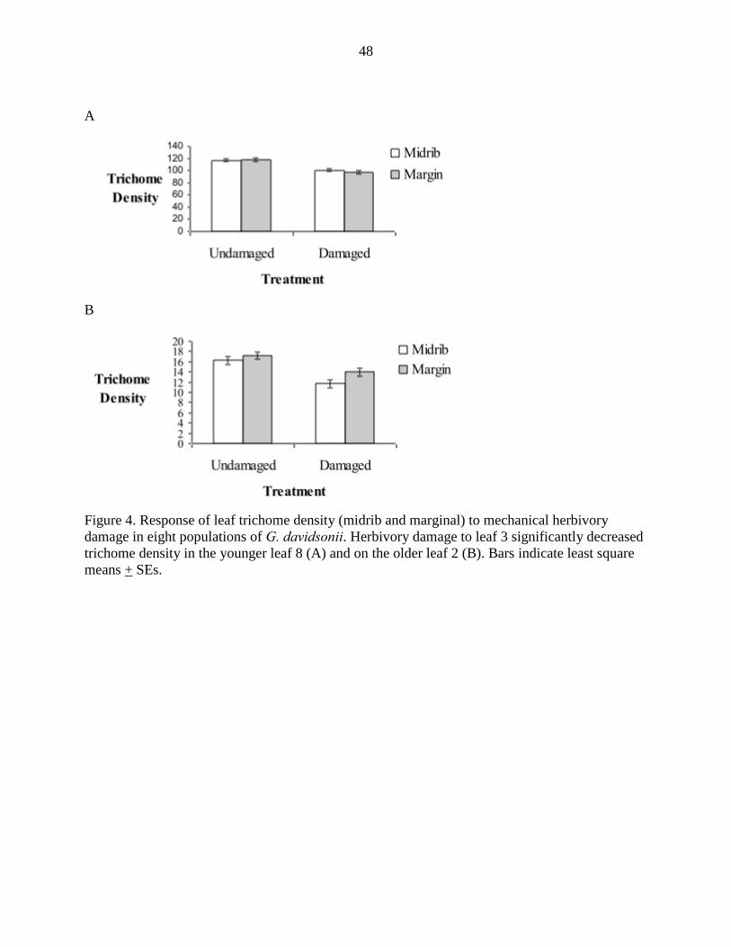
48

A

B

Figure 4. Response of leaf trichome density (midrib and marginal) to mechanical herbivory

damage in eight populations of G. davidsonii. Herbivory damage to leaf 3 significantly decreased

trichome density in the younger leaf 8 (A) and on the older leaf 2 (B). Bars indicate least square

means + SEs.

49

A

B

Figure 5. Water, nutrient, and water x nutrient environments did not significantly affect average

(A) or population-specific (B) foliar gossypol expression in G. davidsonii. Bars indicate least

square means + SEs. We detect a significant population effect, though no population x

environment effects were detected.

[Gossypol]

(mg/g)

Population

50

Figure 6. Average response of lysigenous cavity density to water x nutrient environments in G.

davidsonii. Cavity density was significantly higher under low water conditions than high. High

nutrient conditions produced marginally larger amounts of lysigenous cavities than low

conditions. Water x nutrient effects were not significant. Bars indicate least square means + SEs.

Figure 7. Average response of leaf (midrib) trichome density to Water X Nutrient environments

in G. davidsonii. The effect of nutrients was marginally significant; no other significant effects

were detected. Bars indicate least square means + SEs.

Supplemental Information

51

Table S1. Analysis of Variance for Leaf 8 Responses to Herbivory Experiment. Shown are the

defense responses (Response), Sources of Variation, Degrees of Freedom (DF), Effect size in

comparison to the total model, F Ratio and P values from the F-test. The effect size for the total

model is the total amount of variation explained by the model.

Response Source DF Effect Size (%) F Ratio P

Leaf Cavity Density

Population 7 24.53 1.0357 0.4136

Damage 1 38.37 11.3407 0.0012

Damage*Population 7 7.71 0.3255 0.9402

LEAF 8 LENGTH 1 33.19 9.8089 0.0025

PLANT HEIGHT 1 0.11 0.0321 0.8582

LEAF 2 LENGTH 1 0.91 0.2686 0.6058

Total Model 18 28 1.642 0.0706

Total 94

Gossypol Leaf Concentration

Population 7 71.49 4.5273 0.0002

Damage 1 13.12 5.8174 0.0179

Damage*Population 7 9.2 0.5823 0.7687

LEAF 8 LENGTH 1 8.09 3.5878 0.0614

PLANT HEIGHT 1 0.05 0.0258 0.8728

LEAF 2 LENGTH 1 1.47 0.6529 0.4212

Total Model 18 33 2.4626 0.0028

Total 108

Leaf Trichome Density

Population 7 35.14 1.7837 0.101

Damage 1 37.96 13.4876 0.0004

Damage*Population 7 14.1 0.7156 0.6589

LEAF 8 LENGTH 1 12.16 4.3208 0.0407

PLANT HEIGHT 1 1.96 0.6959 0.4065

LEAF 2 LENGTH 1 6.42 2.2799 0.1348

Total Model 18 29.48 1.974 0.020

Total 103

52

Table S2. Analysis of Variance for Leaf 2 Responses to Herbivory Experiment. Shown are the

defense responses (Response), Sources of Variation, Degrees of Freedom (DF), Effect size in

comparison to the total model, F Ratio and P values from the F-test. The effect size for the total

model is the total amount of variation explained by the model.

Response Source DF Effect Size (%) F Ratio P

Leaf Gland Density

Population 7 69.18 3.4705 0.0029

Damage 1 6.43 2.2591 0.1372

Damage*Population 7 18.35 0.9204 0.496

LEAF 8 LENGTH 1 4.13 1.4499 0.2325

PLANT HEIGHT 1 10.47 3.6757 0.0592

LEAF 2 LENGTH 1 8.6 3.02 0.0865

Total Model 18 32.78 1.951 0.0244

Total 90

Leaf Gossypol Concentration

Population 7 76.76 12.3814 <.0001

Damage 1 0 0.0014 0.9703

Damage*Population 7 7.39 1.1924 0.3158

LEAF 8 LENGTH 1 0.17 0.1972 0.6581

PLANT HEIGHT 1 0.04 0.0407 0.8406

LEAF 2 LENGTH 1 0.51 0.5737 0.4508

Total Model 18 56.77 6.273 <.0001

Total 104

Leaf Trichome Density

Population 7 28.25 1.3592 0.2336

Damage 1 15.03 5.061 0.0271

Damage*Population 7 11.43 0.55 0.794

LEAF 8 LENGTH 1 8.18 2.7547 0.1007

PLANT HEIGHT 1 6.08 2.0459 0.1564

LEAF 2 LENGTH 1 4.69 1.5789 0.2124

Total Model 18 28.86 1.8709 0.0298

Total 101

53

Table S3. Analysis of Variance for Responses to the Nutrient x Environment Experiment. Shown

are the defense responses (Response), Sources of Variation, Degrees of Freedom (DF), Effect

size in comparison to the total model, F Ratio and P values from the F-test. The effect size for the

total model is the total amount of variation explained by the model.

Response Source DF Effect Size (%) F Ratio P

Leaf Cavity Density

Population 5 42.6 8.386 <.0001

H20 1 33.04 32.5237 <.0001

Nutrient 1 5.36 5.2717 0.0254

H20*Nutrient 1 0.03 0.0343 0.8537

Population*H20 5 16.32 3.2123 0.0127

Population*Nutrient 5 14.68 2.8895 0.0215

Population*H20*Nutrient 5 17.52 3.4489 0.0086

Total Model 23 63.33 4.2795 <.0001

Total 80 Gossypol Leaf

Concentration

Population 5 57.17 4.1212 0.0029

H20 1 2.66 0.9586 0.331

Nutrient 1 3.65 1.3141 0.2564

H20*Nutrient 1 0.45 0.1612 0.6896

Population*H20 5 4.02 0.2899 0.9167

Population*Nutrient 5 13.25 0.9552 0.4529

Population*H20*Nutrient 5 5.21 0.3759 0.8632

Total Model 23 38.74 1.5675 0.0862

Total 80

Leaf Trichome Density

Population 5 16.57 0.8519 0.5193

H20 1 3.14 0.8068 0.373

Nutrient 1 15.2 3.9066 0.0532

H20*Nutrient 1 4.01 1.0315 0.3143

Population*H20 5 22.53 1.1586 0.3415

Population*Nutrient 5 28.08 1.4438 0.2236

Population*H20*Nutrient 5 11.4 0.5859 0.7106

Total Model 23 32.25 1.1178 0.358

Total 80

54

CHAPTER 3. Response of herbivory to defense traits, geographic and genetic structure

within a Sonoran Desert wild cotton species, Gossypium davidsonii

A paper to be submitted to Perspectives in Plant Ecology, Evolution and Systematics

Adam Kuester and John D. Nason

Abstract

Understanding the evolutionary mechanisms and patterns of natural plant defenses

can yield insight into controlling pest populations and directing breeding programs for

defense traits that exert resistance to crop pests. We observed the effects of genetic structure

detected by neutral simple sequence repeat loci, geographic distance between individual

plants, and trichome and gossypol-glanded quantitative phenotypes on both leaf and seed

damage in four populations of Gossypium davidsonii. We detected fine-scale genetic

structuring within populations and tradeoffs in defense traits (foliar trichome density and leaf

and seed gossypol gland density). Using multiple regressions on dissimilarity matrices, we

investigated effects of inter-plant geographic, genetic and phenotypic distances within 4 large

populations of G. davidsonii on herbivore damage (both leaf and seed damage) across

populations. We found no common important effect on leaf or seed herbivory, which likely

reflects the environmental diversity in sampled field sites.

Key Words: Gossypium, plant defense, fine scale genetic structure, multiple regressions on

distance matrices

55

Introduction

Recognizing the mechanisms and patterns of evolution of natural plant defenses not

only allows us to understand how to reasonably control host associated pest populations, but

also to direct better-suited breeding and selection programs for traits associated with

tolerance or resistance to otherwise uncontrollable pests (Gould 1988, Cortesero et al. 1999,

Rausher 2001, Thrall et al. 2011). Plant resistance traits to insect pests may comprise several

divergent defense mechanisms. Variation in chemical defense quantity and composition can

affect the degree to which a specialist insect herbivore associates with host plants both

among and within populations (Berenbaum and Zangerl 2006, Zangerl et al. 2007). Other

plant defenses, such as pubescence, can be useful as physical deterrents against many sap-

feeding and chewing insects (Andres and Connors 2003, Franks et al. 2008, Neves et al.

2010). In cases where indirect defenses from higher trophic levels aid in plant defense, such

as volatile organic compounds that signal to parasitoid or predatory insects, or extrafloral

nectaries, which utilize myrmecophyllic interactions with associated ant species in protecting

the plant against herbivory (Pare and Tumilson 1999, Engelberth et al. 2003, Heil and

McKey 2003, Kaminski 2008), interaction between plants and other insects may provide the

most efficient defense against associated herbivores.

Tradeoffs in defense trait investment are often observed in nature, possibly to direct

additional resources to growth and reproduction (Lerdau et al. 1994, Donaldson et al. 2005,

Agrawal 2006). Tradeoffs can sometimes be nearly immediate events, whereby resource

reallocation occurs in young tissues of the attacked plant, or can take several generations via

microevolution of particular defense combinations (Baldwin et al. 1998, Bezemer et al. 2005,

56

Bolton 2009, Aharoni and Galili 2010). The latter mechanism would heavily depend on a

non-plastic genetic basis for trait variation.

Insects can interact with plants in a variety of ways on many different scales. Some

insects, such as generalist pollinators (Waser et al. 1996, Johnson and Steiner 2000) or

herbivores with broad diets (Pennings et al. 1993, Bernays and Minkenberg 1997, Hagele and

Rowell-Rohier 1999), benefit from interactions with an array of plants. In cases where insect

species have generalized host preferences, certain herbivore populations may prefer only one

or a few hosts (Via 1990). Host preference across an insect herbivore’s species range can

arise initially from host availability and distribution (Visser 1988), but also can stem from

variation in host plant phenotypes (Thompson 1991, Zangerl 1993, Feder et al. 1994, Mopper

and Simberloff 1995). Often, an insect-plant interaction results from some combination of

plant phenotypes, whereby a certain phenotypic syndrome enables or disables the interaction.

Insects within a plant population may favor specific combinations of plant traits, leading

eventually to further host specificity and population differentiation.

Though generalist herbivores may have localized phenotype preferences for certain

plant species or ecotypes, so can specialist insect herbivores on a particular host species

(Pashley 1993). Population-level adaptations of insects to host plant populations (Berenbaum

1998; Thompson 2005) can lead to specialization for particular plant phenotypes, such as

phenology (Feder 1994, Mopper 2005) and floral characteristics (Anderson and Johnson

2008, Herrera and Bazaga 2007, Anderson and Johnson 2009), but often to defense

syndromes as well (Zangerl and Berenbaum 1993, Agrawal 2004; Awmack 2002, Mopper et

al. 2000).

57

Insects can select for specific defense traits within plant communities (Strauss and

Zangerl 2002, Lankau 2007). Inter-population variation in plant defense has been attributed

to varying herbivore pressures (Ward et al. 1997, Valverde et al. 2001). Variation may be

linked to tradeoffs, be they molecular (Rojo et al. 2004, Spoel et al. 2007), energetic (Zangerl

and Berenbaum 1997, Agrawal 2002) or ecological (Strauss et al. 2002), that result from the

plastic responses to changing environmental conditions.

Defense trait variation within local populations can have varying degrees of fitness

consequences for a plant depending on how associated insect herbivores respond to the

varying levels of plant defense. Variation in defense syndrome may be a response to

tradeoffs among traits as a result of variable environmental effects. Often, a plant responds to

more than one herbivore, in addition to more than one type of environmental stress, within a

temporally and spatially dynamic pattern of herbivory. In addition to herbivore response,

plants endure varying abiotic conditions, nutrient availability, and pathogenic responses, all

of which contribute to one perceived defense syndrome.

When an insect herbivore is hosted by a few to many species, there is usually trait

variation among hosts. In particular, defense phenotypes can vary among closely related

species. For instance, in the genus Gossypium (family Malvaceae), there is marked variation

in several defense phenotypes, including trichome density on different aerial plant parts,

phytochemical defenses, both in composition and quantity in above and belowground plant

parts, and extrafloral nectaries (Stipanovic 2005, Rudgers 2004, Kahn 1988). Rudgers et al.

(2004) recognized significant tradeoffs in plant defenses amongst species within the genus, in

addition to within species intra-population tradeoffs.

58

Defense trait variation may, in fact, create quite different responses by associated

insect herbivores. For instance, several seed-feeding insects, regarded as specialist herbivores

that rely on Gossypium plants for development, have been shown to be attracted by particular

colors of cotton leaves and high levels of plant terpenoids (Lincoln and Boyer 1975, Hedin

and McCarty 1995), whereas generalist folivores tend to tolerate lower levels of plant toxins

and varying degrees of leaf pubescence depending on feeding habit. Additionally, cotton

plants produce extrafloral nectaries for myrmechophilic relationships with associated ants,

which can contribute substantially to plant defensibility in certain cotton species (Rudgers et

al. 2004).

Herbivory levels on plants may be a result primarily of plant defense phenotypic

syndromes, but likely result from a combination of plant genetic structure (Wimp et al. 2004,

Hochwender and Fritz 2004), spatial distribution (Morris and Kareiva 1989), temporal

outbreak dynamics (Speer et al. 2001) and host apparency by associated herbivores (Chew

and Courtney 1991). Our objective within this study is to address the relative importance of

genetic relatedness, geographic proximity, and differences in defense phenotypes on plant

herbivory both in leaves and seeds, and to better understand why and how a plant uses

different defenses against associated herbivores. In addition, we will address the degree to

which tradeoffs of defense phenotypes are apparent within the system.

Methods

Gossypium davidsonii, a wild cotton species endemic to the Baja California

Peninsula, was used for analyses of plant defense evolution. Large populations of nearly 50

individuals were chosen, representing the range of the species. In particular, we chose two

59

populations in the north and two in the southern portion of G. davidsonii’s range (Figure 1).

Like most cotton species, G. davidsonii has several means of defense against herbivory. Most

importantly, we have noted that trichome densities on aerial plant parts and gossypol

lysigenous cavity production on vegetative and reproductive parts have large variation within

and among populations of the species (Phillips and Clements 1967, Kuester and Nason, in

prep), which may be in response to varying herbivore environments. Though extrafloral

nectaries have been widely utilized as a defense in some cotton species (Rudgers et al. 2004),

we see very little presence of associated ants and little production of nectar within wild

populations of G. davidsonii (pers. obs.).While some trait variation may be a result of

environmental conditions, defense traits have been shown to exude high levels of heritability

within the genus (Lee et al. 1973) as well as to be minimally affected by extreme

environmental conditions in glass house experiments (Kuester and Nason, in prep); therefore,

we believe that defense traits have strong genetic control for which spatial dynamics and

genetic structure may greatly affect herbivory levels on plants and ultimately plant fitness.

Genetic Material

Plant Material- Four fully expanded healthy leaves, randomly collected from each

plant, were dried whole in silica gel for preservation and then stored at -80 °C for later

phenotypic analyses. One expanding leaf was selected per individual and stored in silica gel

at -80 °C until use for genetic analysis. In total, at least 48 plants were selected per

population. Collections were made in the Fall, 2009.

Seeds from at least three fruits per plant were also collected. Seeds from individual

fruits were packaged separately in coin envelopes. All seeds were inspected by the

60

Secretaría de Ganadería Agricultura Rural Pesca y Alimentación (SEGARPA) prior to

importation to the United States. Permit by the United States Department of Agriculture

(USDA), Plant Protection and Quarantine (PPQ) Permit 562, permitted importation of cotton

seed.

Isolation of DNA- Fifteen milligrams of silica-dried leaf material was used for DNA

isolation. The leaf tissue was ground using the Genogrinder 2000 then extracted using the

Autogenprep 740 DNA extraction robot (Holliston, MA) at the Iowa State University DNA

Facility. All DNA samples were eluted in water. Concentration of DNA was determined by

spectrophotometry and dilutions of 20 ng/ μl were prepared for use in Polymerase Chain

Reactions (PCR).

SSR loci- All primers were designed by Integrated DNA Technologies (Corralville,

IA). Of 50 Simple Sequence Repeat (SSR) loci screened from the Cotton Marker Database

(www.cottonmarker.org), 10 were identified as being polymorphic in G. davidsonii (Table 1).

Forward primers were attached to an M13-tagged sequence (Schuelke 2000), used for cost-

effective fluorescent allele calling. A mixture of the sense primer and labeled M13 tag primer

were combined in a ratio of 15 labelled M13-tailed primer to 1 sense primer.

Polymerase Chain Reaction (PCR) - As fragment size overlap precluded running all

10 SSR loci together in one reaction; they were split into three multiplexes of three or four

loci each. PCR and genotyping multiplexes were as followed: Multiplex1: 2 μM GD1, and 3

μM each of GD2 and GD3; Multiplex2: 2 μM GD5, and 3 μM each of GD6, and GD4;

Multiplex3: 3μM each of GD7, GD8, GD9 and GD10. For each reaction, 40 ng of genomic

DNA was used in 10 μl reactions with 0.2 μM Promega (Madison, WI) dNTPs, 2.5 μM

MgCl2 (Bioline (Tauton, MA)), 1X NaCl Buffer (Bioline), and 0.4 units Bioline Taq DNA

61

Polymerase. A MJ Research (Waltham, MA) Programmable Thermal Controller-100

thermocycler was used for all PCR reactions. Thermocycler conditions consisted of 95°C for

3min; 35 cycles of 94°C for 30 s, 50°C for 90 s, 72°C for 60 s; and a final extension at 72°C

for 10 minutes. Samples that failed to amplify were run a second time. One μl of PCR

product was used for fragment detection using an Applied Biosystems 3730 DNA Analyzer

at the Iowa State University DNA Facility. An ABI GS500 size standard was used for

fragment length comparison. All sample genotypes were analyzed using Applied Biosystems

PeakScanner 1.0 analytical software. A PP (Primer Peaks adjustment) sizing default was used

for the analysis.

Fitness Measurements- Proportion of foliar and fruit (seed damage) herbivore damage

was assessed from randomly selected fruits and leaves (described below) from each

individual plant. Proportion of damaged seed was used as a fitness measure of reproductive

success and as a means of detecting selection on measured traits (see “Detecting Selection”

in Data Analysis below). Each marked plant was assessed for both leaf and fruit damage,

with the exception of plants where fruits were not present. The fruit and leaf damage

estimates were only performed during the Fall, 2009, across 4 populations.

Fruit Damage Estimation- For fruit sampling, we first divided a plant into 8 sections,

equally sectioning it in 3 dimensions. Ten fruit per plant were selected, sampling one of 8

sections at random from a random numbers table. From one of the eight sections, we tried to

sample fruit with a full seed set. The proportion of undamaged seed was quantified by

counting number of undamaged seed out of the total seed count per fruit.

62

Leaf Damage Estimation- Eight fully-expanded leaves were randomly selected from

plants. From each of 8 equally-divided sections from a plant (described above), we collected

1 leaf at random. Leaves were photographed and then total leaf area and damaged area

(chewed sections) were measured using ImageJ (Rasband 1997-2011).

Plant Trait Quantification

Seed Lysigenous Cavity Density- At least 10 fruit per plant (when available) were

collected. Three seeds per fruit (three fruit per plant) were quantified for lysigenous cavity

density. Seeds were cut longitudinally and lysigenous cavities were counted per seed half

using an Olympus (Center Valley, PA) dissecting microscope. Longitudinal sections were

also photographed with a Nikon Coolpix (Melville, NY) camera and section areas were

measured in ImageJ (Rasband 1997-2011). Seed collections were made in the Fall, 2009.

Leaf Lysigenous Cavity Density- We quantified foliar lysigenous cavity density from

leaf material dried in silica gel under 2.5 X magnification with an Olympus SZ61 (Center

Valley, PA) microscope. Three samples from three separate leaves were counted in order to

estimate an average cavity density (# per mm2 area) per plant.

Leaf Trichome Density- We quantified trichomes from leaf material dried in silica gel

under 2.5 X magnification with an Olympus SZ61 (Center Valley, PA) microscope. Silica

gel preservation of leaf material had no apparent damage to leaf trichome quantification (pers.

obs.). Three samples from three separate leaves were counted (# per mm2) in order to

estimate an average leaf trichome density per plant.

63

Data Analysis

Distance matrices- Within-population Euclidean pair-wise genetic and geographic

distances were calculated in GenAlEx v. 6.1 (Peakall and Smouse 2006). Geographic

distances were recorded in Universal Transverse Mercator (UTM). Phenotypic datasets per

population were assessed for normality in JMP v. 9, using the Shapiro-Wilks W test. Since

some phenotypic traits within certain populations significantly deviated from normality (see

Results), we used the log of each trait to normalize the datasets and then took the absolute

value between inter-individual differences as a phenotypic distance. We used an arcsin

square-root transformation of raw damage data estimates to adjust for proportion data. The

absolute value of the difference between individual damage estimates was then calculated.

F-Statistics- We calculated observed (HO) and expected heterozygosity (HE), number

of alleles were estimated using GenAlEx (Smouse and Peakall 2006) and inbreeding

coefficient (FIS) for each microsatellite locus using FSTAT (Goudet 2001). An exact test for

Hardy Weinberg Equilibrium for each locus and population was performed using GenePop v.

3.1 (Raymond and Rousset 1995).

Multiple regression on distance matrices- We assessed the relative effect of genetic,

geographic, and phenotypic dissimilarity on both seed and leaf damage using multiple

regressions on distance matrices (MRM, Legendre and Legendre 1998). MRM extends

principals of the partial Mantel test, with the ability to evaluate relationships between

multivariate response matrices on explanatory distance matrices (such as phenotypic, genetic

and geographic distances measured in this study). We also assessed the relative importance

of each explanatory variable by using percent of variance explained by each of the effects of

interest. We detected the “pure effect” of each explanatory variable by following a method

64

described by Krasnov et al. (2010), whereby R2 was estimated leaving the effect of interest

out of the model, and then was subsequently compared to the complete model, using

decomposition. We report percent variance, proportion R2, p-value for each effect, and R

2 for

the entire model. Significance of multiple regressions was estimated with 1000 permutations.

MRM calculations were assessed using the Ecodist package (Goslee and Urban, 2007) in R

(R Development Core Team, 2005). Overall model R2 values were low in our analyses (see

Results), which had been recognized in Krasnov et al. (2010) in use of MRM. Krasnov et al.

explained that more important than detecting explanatory power of the entire model was to

detect relative importance of measured variables.

Damage Comparison Among Populations- We compared mean damage across sites

using a Tukey’s Honest Significant Difference (HSD) test in JMP v. 9. Average seed damage

and leaf damaged were compared among sampled sites to determine if there were differences

in the levels of herbivory across sites.

Tradeoffs in Defense Traits- To assess tradeoffs in plant defenses for each sampled

population, we used the Multiple Regression on Matrices test in the Ecodist package (Goslee

and Urban 2007) in the R program, testing for a relationship between pair-wise phenotypic

distance matrices, having taken into account geographical and genetic pair-wise differences

(probability denoted PM in the text). We assessed the significance of linear regressions of

each trait, using the fit Y by X function in JMP v. 9, and report the significance of the slope

of the regression (probability denoted PR in the text).

We also assessed pair-wise tradeoffs in defense traits, taking into account genetic

distance, geographic distance and whether or not boll weevils were present or absent at each

65

of the sites (denoted 0 or 1), on density of trichomes, seed and leaf lysigenous cavities over

all populations using MRM in the Ecodist package in R.

Detecting Selection- We detected directional selection following the approach of Lande and

Arnold (1983). Independent variables (trichome, leaf lysigenous cavity and seed lysigenous

cavity density) were z-standardized with a mean of zero and standard deviation of one. To

detect directional linear selection, relative fitness was regressed over each of the z-

standardized phenotypes. We also detected correlation between z-standardized traits using

Pearson correlation tests.

To quantify non-linear selection (stabilizing, disruptive, and/or correlational

selection), we fit a quadratic term to the regression of relative fitness on each phenotype and

interaction terms between phenotypes. Presence of positive and negative γ coefficients reflect

stabilizing and disruptive selection, respectively. We also found a local maximum or

minimum of the quadratic function to determine the presence of disruptive versus stabilizing

selection. Where interaction terms in the quadratic model were significant, we plotted

relative fitness against each of the two z-standardized phenotypes to interpret the selection

gradient using the scatterplot3d package (Ligges 2012) in the R program.

Spatial Autocorrelation- We assessed spatial autocorrelation for each population of

genetic relationship (r) over the natural log of geographic distance using GenAlEx (Peakall

and Smouse 2006). We also estimated the kinship coefficient (Fij), as described by Raymond

(1995), defined as the relationship of identity by descent, using the formula, option 2, in the

SPAGeDi v. 1.3 software package (Hardy and Vekemans 2002). Average coefficients were

estimated over all loci and significance from the null hypothesis of no relatedness was

determined by comparing to 1000 permutations. We assessed the autocorrelation of Fij with

66

the geographic distance. Though we report only genetic correlation (r) across distance, we

used Fij to estimate the Sp statistic, which is noted to be an effective measurement of fine

scale genetic structure, which does not depend on the sampling strategy (Vekemens and

Hardy 2004). The Sp statistic was calculated as bk/(r-1), where bk is the regression slope of

the kinship coefficient with the natural log of geographic distance, and r is the average

kinship coefficient. The Sp statistic can be easily used to compare among populations with

different patterns of spatial distribution, as noticed within this study, so as to compare genetic

structuring among populations (Vekemans and Hardy 2004).

We further examined spatial autocorrelation across all 4 populations using the

heterogeneity test in GenAlEx (Peakall and Smouse 2006), which compares the correlation

coefficient of genetic relatedness (r) over geographic distance (here we used 10 meter

distance intervals) across sites and tested the null hypothesis of no correlation between

genetic relatedness and geographic distance.

Spatial autocorrelation of defense traits (pair-wise phenotypic distances) over

geographic and genetic distance were also assessed for each studied population using

GenalEx.

Results

Normality test of phenotypes within populations- When assessing for normality of

phenotypic datasets, we found little evidence for deviation from a normal distribution for

most traits across populations, with exception of leaf lysigenous cavities (W= 0.941, P =

0.015) and trichome densities (W= 0.862, P =0.001) for site WC, and seed lysigenous cavity

density for sites SB (W= 0.924, P =0.0042) and 96 (W= 0.845, P = 0.001).

67

F-Statistics- The number of alleles per locus over all 4 populations ranged from 5-17

(Table S1, mean = 9). The expected (HE) and observed (HO) heterozygosity estimates ranged

from 0.15- 0.492 (Table S1, mean 0.292) and 0.436- 0.734 (Table S1, mean 0.620),

respectively. Estimates of FIS ranged from 0.07- 0.743 and the overall FIS was highly

significantly greater than zero (Table S1, mean 0.535, P <0.001). Estimates of FST ranged

from -0.003-0.138 and the overall estimate was significantly greater than zero (Table S1,

mean 0.06, P <0.001). All loci and populations deviated from HWE.

Multiple Regressions on Dissimilarity Matrices- The multiple regressions of

dissimilarity matrices of plant damage, both proportion of seeds damaged per fruit and

amount of leaf area damaged, against matrices of genetic, geographic, and defense trait

phenotypic (seed and foliar lysigenous cavity and foliar trichome densities) distances for

each of 4 populations demonstrated significant models across all sites, though the number

and relative importance of significant explanatory variables varied by site and dependent

variable (Table 2).

We found no similarity in relative importance of measured effects on seed damage

within sites where boll weevils were or were not present. In particular, we found that in site

SB, seed gland and leaf gland density were significantly positively correlated with seed

damage, while in site 96 we only detected a significant positively correlated effect of

trichome density with seed damage. In the southern sites, we observed smaller, or even no

significantly correlated effects on seed damage. Where we found no significant effect on seed

damage in site WC (Table 2), we likewise observed very low variation in seed damage across

plants (Figure 3).

68

We found one significant correlation between a measured effect and leaf damage

across each of four sites (Table 2). We noted two occurrences of a significant correlation of

genetic relatedness on leaf damage, though with opposite signs (sites positively correlated in

TC and negatively correlated in SB). Geographic patterning of plants was the only significant

correlation at site 96. The only defense phenotype with significant correlation with leaf

damage was seed gland density at site WC.

Phenotypic correlations- Leaf trichome and cavity density were positively correlated

in the two southern sites (Figure 2 TC: R= 0.311, PM= 0.014, PR= 0.014; WC: R=0.431, PM=

0.001, PR< 0.001). We also found a negative correlation between trichome and seed

lysigenous cavities (Figure 2 TC: R= -0.104, PR= 0.554, PM= 0.004, WC: R= -0.168, PM=

0.475, PR= 0.285) and between leaf and seed lysigenous cavities (Figure 2 TC: R= -0.206,

PR= 0.213, PM= 0.006; WC: R= -0.245, PM= 0.001, PR= 0.233) in site TC using MRM.

We found no significant correlation between trichome and leaf lysigenous cavity

density within either northern site (Figure 2 SB: R= 0.151, PM= 0.019, PR= 0.467; 96: R=

0.036, PM= 0.850 PR= 0.924). We also found a negative correlation between leaf and seed

lysigenous cavity density (Figure 2 SB:R= -0.346, PM = 0.009, PR= 0.023; 96: R=-0.133, PM

= 0.174, PR = 0.321) within site SB.

Over all populations, we found a significant correlation, be it weak, between trichome

and leaf lysigenous cavity density (R= 0.21, P = 0.003), a positive correlation between

trichome and seed lysigenous cavity density (R = 0.53, P = 0.013), but no correlation

between leaf and seed lysigenous cavity density (R = 0.123, P = 0.368) having taken into

account variation attributable to genetic, geographic, and boll weevil presence dissimilarities

using MRM.

69

Detecting Selection – We found directional selection favoring higher levels of seed

lysigenous cavity densities at site 96 (β = 0.100, R2

= 0.056, P = 0.027), but lower levels of

seed lysigenous cavity densities in site WC (β = -0.053, R2

= 0.047, P = 0.079). We detected

a signature of stabilizing selection for trichome density (γ = -0.098, P = 0.0229) and

correlative selection for low levels of trichomes and high levels of leaf lysigenous cavities (γ

= -0.1581, P = 0.004) in site 96. The only other signature of selection found was disruptive

selection for seed lysigenous cavity density in site SB (γ = 0.088, P = 0.0391).

Spatial Autocorrelation and Fine Scale Genetic Structure-Though we observed little

effect of geography on either response variable in the multiple regression of dissimilarity

matrices, we observed significant fine scale genetic structure (FSGS) for G. davidsonii at

three of four site locations (Table 2). Of the four populations, site TC exhibited FSGS at finer

scales than other sites (Figure 3). We also observed a significant and largest measured effect

of genetic dissimilarity on foliar damage rates and a proportionally large and significant

effect of geographic dissimilarity on seed attack rates within this site (Table 2).

In the two other sites where we detected significant FSGS, genetic structure was only

evident at larger geographic scales (Figure 3 WC and SB: 10m). In site 96 we did not detect

any significant FSGS. Neither did we observe any significant coefficient of regression when

plotting relatedness estimates over distance (Figure 3d), though we noticed significantly

negative coefficients of regressions on inter-individual genetic relationships at the other three

site locations (Figure 3 a-c).

We noticed 3 sites had similar Sp values, all showing comparable levels of FSGS (TC:

0.0252, WC: 0.0223, SB: 0.0228). Site 96 had an observed Sp an order of magnitude lower

(Sp= 0.0045).

70

We only found significant phenotypic spatial autocorrelation within site SB for leaf

lysigenous cavity density at 25 meters (Figure S1). Likewise, we found significant genetic

autocorrelation of trichome density over genetic distance at a distance of 9.5 within SB

(Figure S2). No other trait x population combination produced any pattern of spatial or

genetic autocorrelation.

Discussion

Our objective within this study was to determine the relative importance of defense

trait variation, genetic relatedness, and spatial distributions within four populations of G.

davidsonii on plant herbivory both in leaves and seed. We also sought to better understand

why and how a plant uses different defenses against associated herbivores. We found that

the importance of a particular plant defense (Table 2) and that the nature and presence of

selection differed among sites. Variation in selective pressures across sites likely impact the

degree to which any one of the studied effects may be of importance.

Gossypol-glanded and trichome phenotypes have been recognized as genetically-

based heritable traits (McMichael 1960, Lee et al. 1973, Wright et al. 1999) in lines of G.

hirsutum, and defense trait variation within G. davidsonii has been noted to be predominantly

attributed to inter-population variation (Kuester and Nason, in prep). We observed no

significant effect of genetic relatedness on seed damage within any of the four study sites.

Likewise we observed little autocorrelation between phenotypic and genetic distance (with

one exception at site SB).

We found that seed gossypol lysigenous cavity density was a poor predictor of seed

damage across sites, with the exception of detecting a large effect size of seed lysigenous

71

cavity density on seed predation within site WC. Because known specialist insect herbivores

on cotton can tolerate, metabolically alter or are stimulated for oviposition by gossypol and

related terpenoids (Stipanovic et al. 2008, Hedin and McCarty 1995), we had anticipated that

damage rates would be a direct response to gossypol levels in seed.

We expected to find differing responses to seed predation across sites, as diverse

pressures on fruit and seed damage occur between northern and southern populations of G.

davidsonii (Figure 3; pers. obs.). In particular, in the southern two sites, where we frequently

find the boll weevil, a cotton fruit and seed specialist that was noted to attack over ¾ of

damaged fruits at studied sites, we had expected to find significant and large effects of

gossypol lysigenous cavity phenotypes and foliar trichomes on seed damage, as these effects

have been previously identified in feeding trials and field studies on A. grandis associated

with G. hirsutum (Parnell 1949, Hedin and McCarty 1995).

Seed lysigenous cavity and trichome density were relatively large effects on seed

damage in the WC site, which make sense in the context of boll weevil attack. For site TC,

we noticed a relatively large effect of geography on seed damage. We also found the largest

effect of genetic relatedness on damage within this population. It is possible that boll weevils

reproduce on or near natal host plants, as is the case on volunteer cotton in cultivated fields

(Showler et al. 2009), though it is not clear why the insect would not disperse to oviposit

within a larger cotton-dominating landscape within the TC site or throughout the southern

region where boll weevils are found. Female boll weevils may be selecting for specific

genotypes of cotton. We do observe relatively large genetic differentiation among boll

weevils collected at ten cotton sites within the los Cabos of the Baja Peninsula (Kuester et al.

in prep), which may suggest that individuals restrict travel to on or near natal plants, even

72

though cotton resources are abundant across the region (pers. obs.). The only other observed

fruit damage in either site was from a specialized Lepidopteran species, present at all studied

sites and was the predominant fruit attacker in the north.

The fact that the largest effect on seed damage at site 96 was geographic distance

makes sense, as plants were sparsely distributed along a matrix of washes. Presumably, the

specialist Lepidoptera that hatches and feeds during larval development on cotton fruit (and

subsequently seed), would have geographic patterns for host oviposition, as search patterns in

insects are often affected by geographic structuring of the host (Morris and Kareiva 1989).

Interestingly, in site SB, which consists of a dense and nearly continuous patch of cotton, the

largest effect on seed damage in SB was foliar trichome and seed lysigenous cavity density.

It is unclear how trichomes impact Lepidoptera feeding, as the species has not been observed

feeding on leaves (pers. obs.).

The important effects on leaf damage across sites TC, WC and SB appeared to be

similar, in that seed lysigenous cavity density, genetic similarity, and seed damage were

common significant effects. Because green leaf volatiles from cotton leaves are known to

enhance the aggregation pheromone of boll weevils (Whitman and Eller 1990), we might

anticipate a large effect of seed lysigenous cavity density or seed damage as being linked to

foliar damage in the two southern populations.

We observed nearly all of the observed effect at site 96 attributable to geography,

which makes sense given the sparse plant distribution along washes at the site and that we

observed no specialist leaf feeding insects at any site across the range of G. davidsonii (pers.

obs.). Generalist herbivores often feed in geographic patterns (Visser 1988), which may

73

reflect a heterogeneous distribution of generalist herbivores at the site, perhaps in relation to

plant community densities.

We detected selection for high levels of seed lysigenous cavity density in one

northern site. Though gossypol is tolerable in many cotton specialists and even attracts some

host associated herbivores, it is possible that the larvae that develop within fruit capsules of

G. davidsonii plants have low tolerance for it. Stipanovic et al. (2008) have shown that

several generalist herbivores have decreased fitness (longer developmental times) when fed

artificial diet containing the compound. Plants may have higher reproduction if it adequately

defends itself against granivores when producing higher levels of gossypol-related

phenotypes.

On the other hand, at another northern site (site SB), we detected disruptive selection

for seed lysigenous cavity density. Selection in favor of low or high levels of chemical

defenses may be in response to patchy association of herbivore communities within the site.

Where few herbivores are present, plants with lower levels of defense investment may be

able to have high levels of reproductive output. At site WC, where nearly all seed attack

(nearly ¾) was attributable to boll weevil feeding, selection favored lower levels of gossypol.

Plants expressing lower levels of gossypol-related traits may be less attractive to boll weevils,

and in turn, produce more viable offspring.

We also found a signature of stabilizing selection on trichome density and correlative

selection between trichome and leaf lysigenous cavity density at site 96. Since trichomes are

useful physical deterrents against many chewing insects, they may be useful at site 96 where

highest levels of foliar attack were observed (Figure 3b). Production of high levels of

lysigenous cavities, on the other hand, would result in a tradeoff with trichome production.

74

Correlative selection appeared to favor high levels of leaf lysigenous cavities and low levels

of trichomes. We see no clear tradeoff between leaf lysigenous cavity and trichome densities

at the (Figure 2j); however, which might indicate that either the selection surface is too

shallow to exhibit strong relationships between phenotypes or that non-additive genetic

effects are contributing to variation in these defense traits within the population. Since

lysigenous cavity and trichome phenotypes have been recognized as heritable traits

(McMichael 1960, Lee et al. 1973, Wright et al. 1999) within the genus Gossypium, the latter

would not appear to plausibly contribute greatly to inter-plant differences in leaf defense

phenotypes.

Interestingly, we noticed a significant tradeoff between leaf and seed gossypol

lysigenous cavity density across all sites. This may reflect metabolic or energetic constraints

for a plant to produce high levels of defenses across tissues. We only noticed a significant

effect of leaf attack on seed attack in sites WC and SB (WC: r = 0.288, P = 0.006; SB: r=

0.342, P = 0.002), which may suggest similar patterning of seed and leaf foraging in those

sites. For sites where attack on seed and leaves are correlated, it is unclear whether we may

expect a tradeoff between leaf and seed gossypol. Tradeoffs to protect more valuable

reproductive tissues would seemingly be advantageous. In both sites we either saw

significant or marginally significant effects of seed and leaf lysigenous cavity density on seed

predation. Contrary, we find no association of defense phenotypes on foliar attack.

Boll weevils are attracted to gossypol for female oviposition (Hedin and McCarty

1995) and damaged seed by seed feeding insects on cotton are known to germinate quicker

than undamaged seed (Karban and Lowenberg1992). Since boll weevils may impact G.

davidsonii plants both positively and negatively, we might anticipate selection for mean

75

gossypol-related traits where boll weevils are present. Selection within site TC was directed

for higher levels of trichomes, which may reflect the resistance of pubescence on boll

weevils (Parnell 1949), though at site WC we observed no signature of selection.

We noticed similar trends in defense correlations in northern sites where the boll

weevil was not found and in southern sites, where the predominant fruit attacker was the boll

weevil. Specifically, we found significant positive relationships between foliar lysigenous

cavity and trichome density and trends for negative correlation between foliar trichome and

seed lysigenous cavity density in southern sites. Seed lysigenous cavity density and leaf

trichome density levels may affect the degree to which boll weevils attack cotton plants, as

both foliar trichomes and glanded phenotypes are understood to affect levels of boll weevil

attack (Hedin and McCarty 1994, Parnell 1949). In particular, we would have expected plants

to tradeoff greater trichomes (which inhibit boll weevil oviposition) for glanded phenotypes

(which attract boll weevils for oviposition) in the presence of boll weevils if they negatively

affected plant fitness.

In northern sites, we observe a positive correlation between trichome and seed

lysigenous cavity density phenotypes. Trichomes affect first instar larval mobility within

pink bollworm (Pectinophora gossypiella) (Medeiros et al. 2007), though increased

trichomes have minor or even positive effects on Lepidopteran species in general (Rudgers et

al. 2004). While pink bollworm and other specialist insects are resistant to gossypol defenses,

they exhibit reduced fitness when combined defenses are present (Carriere 2004).

In greenhouse experiments, Kuester and Nason (in prep) found large positive

correlations between trichome and both leaf gossypol and gossypol gland phenotypes in

young, 8-leaf stage plants, but found very weak correlations within older, 4-month year old

76

plants, which might suggest that tradeoffs are more apparent in immature plants within this

species. Kuester and Nason (in prep) found that leaf trichome and lysigenous cavity densities

significantly correlated across plants in young leaves of immature plants (8 leaf stage: R2 =

0.167, P <0.001; 4 month old: R2 = 0.07, P = 0.018). Over all 4 populations, we found

positive correlations between trichome density and lysigenous cavity densities, but no

correlation between lysigenous cavities in leaves and seed.

Within this study we found no common effect on plant fitness, which may reflect the

heterogeneous environmental conditions, including herbivore community composition and

structure, present among the investigated sites. We noticed similar correlations within

northern and southern sites, which may reflect similar herbivore environments. Further

investigation of insect community assemblages on wild cotton species, in particular G.

davidsonii, will be needed to understand the extent of herbivore selection for defense traits

within wild species. Moreover, additional inspection of temporal variation in plant defense

and associated damage across seasons will be needed to verify effect patterns.

Literature Cited

Agrawal, A.A., 2004. Plant defense and density dependence in the population growth of

herbivores. American Naturalist 164, 113-120.

Agrawal, A.A., 2005. Future directions in the study of induced plant responses to herbivory.

Entomologia Experimentalis et Applicata 115, 97-105.

Agrawal, A.A., J.A. Lau, P.A. Hamback, 2006. Community heterogeneity and the evolution

of interactions between plants and insect herbivores. Quarterly Review of Biology 81, 349-

376.

Anderson, B., S.D. Johnson, 2008. The geographical mosaic of coevolution in a plant-

pollinator mutualism. Evolution 62, 220-225.

77

Anderson, B., S.D. Johnson, 2009. Geographical covariation and local convergence of flower

depth in a guild of fly-pollinated plants. New Phytologist 182, 533-540.

Berenbaum, M.R., A.R. Zangerl, 1998. Chemical phenotype matching between a plant and

its insect herbivore. Proceedings of the National Academy of Sciences of the United States of

America 95, 13743-13748.

Bezemer, T.M., R. Wagenaar, N.M. Van Dam, W.H. Van Der Putten, F.L. Wackers, 2004.

Above- and below-ground terpenoid aldehyde induction in cotton, Gossypium herbaceum,

following root and leaf injury. Journal of Chemical Ecology 30, 53-67.

Feder, J.L., S.B. Opp, B. Wlazla, K. Reynolds, W. Go, S Spizak, 1994. Host fidelity as an

effective premating barrier between sympatric races of the apple maggot fly. Proceedings of

the National Academy of Sciences of the United States of America 91, 7990-7994.

Goudet, J., 2001. FSTAT, a program to estimate and test gene diversities and fixation indices

(version 2.9.3). [Internet]. Lausanne, Switzerland: Lausanne University; [cited 2012 Nov 18]. Available

from: URL http://www2.unil.ch/popgen/softwares/fstat.htm.

Hardy, O.J., X. Vekemans, 2002. SPAGeDi: a versatile computer program to analyse spatial

genetic structure at the individual or population levels. Molecular Ecology Notes 2, 618-620.

Hedin, P., J. McCarty, 1995. Boll Weevil Anthonomus grandis Boh. Oviposition Is

Decreased in Cotton Gossypium hirsutum L. Lines Lower in Anther Monosaccharides and

Gossypol. Journal of Agricultural and Food Chemistry 43, 2735-2739.

Herrera, C.M., P. Bazaga, 2009. Quantifying the genetic component of phenotypic variation

in unpedigreed wild plants: tailoring genomic scan for within-population use. Molecular

Ecology 18, 2602-2614.

Karban, R., and G. Lowenberg, 1992. Feeding by seed bugs and weevils enhances

germination of wild Gossypium species. Oecologia 92, 196-200.

Khan M.A., J.M. Stewart, J.B. Murphy, 1999. Evaluation of the Gossypium gene pool for

foliar terpenoid aldehydes. Crop Science 39, 253-258.

Krasnov B.R., D. Mouillot, G.I. Shenbrot, 2010. Similarity in ectoparasite faunas of

Palaearctic rodents as a function of host phylogenetic, geographic or environmental

distances: Which matters the most? International Journal for Parasitology 40, 807-817.

Lande, R., S.J. Arnold, 1983. The Measurement of Selection on Correlated Characters.

Evolution 37, 1210-1226.

Lerdau, M., M. Litvak, R. Monson, 1994. Plant chemical defense: monoterpenes and the

growth-differentiation balance hypothesis. Trends in Ecology and Evolution 9, 58-61.

78

Lincoln, C., W.P. Boyer, F.D. Miner, 1975. Evolution of insect pest management in cotton

and soybeans- past experience, present status, and future outlook in Arkansas. Environmental

Entomology 4, 1-7.

Ligges, U., M. Mächler, 2003. Scatterplot3d - an R Package for Visualizing Multivariate

Data. Journal of Statistical Software 8(11), 1-20.

Mopper S., K. Landau, P. Van Zandt, 2000. Adaptive evolution and neutral variation in a

wild leafminer metapopulation. In: Adpative Genetic Variation in the Wild (ed. Mousseau T,

B Sinervo, T Endler), pp. 116-138. Oxford University Press, New York.

Mopper, S., 2005. Phenology- The role of time in structuring space for herbivorous insect

populations. Annales Zoologici Fennici 42, 327-333.

Parnell, F., H. King, D. Ruston, 1949. Insect resistance and hairiness of the cotton plant.

Bull, ent. Res. 39, 539-575.

Peakall, R., P.E. Smouse, 2006. GENALEX 6: genetic analysis in Excel. Population genetic

software for teaching and research. Molecular Ecology Notes 6, 288-295.

Phillips, L., D. Clement, 1967. Variation in the diploid Gossypium species of Baja

California. Madrono 19, 137-147.

Prasifka, J.R., P.C. Krauter, K.M. Heinz, C.G. Sansone, R.R. Minzenmayer, 1999. Predator

conservation in cotton: Using grain sorghum as a source for insect predators. Biological

Control 16, 223-229.

Rasband, W.S., 1997-2009. ImageJ. U.S. National Institutes of Health, Bethesda, MD.

Raymond, M., F. Rousset, 1995. GENEPOP (version 1.2): population genetics software for

exact tests and ecumenicism. Heredity 86, 248-249.

Rojo, E., R. Martin, C. Carter, et al., 2004. VPE gamma exhibits a caspase-like activity that

contributes to defense against pathogens. Current Biology 14, 1897-1906.

Rousset, F., 1997. Genetic differentiation and estimation of gene flow from F-statistics under

isolation by distance. Genetics 145, 1219-1228.

Rudgers, J.A., S.Y. Strauss, J.F. Wendel, 2004. Trade-offs among anti-herbivore resistance

traits: insights from Gossypieae (Malvaceae). American Journal of Botany 91, 871-880.

Schuelke, M., 2000. An economic method for the fluorescent labeling of PCR fragments.

Nature 18, 233-234.

79

Showler, A.T., 2008. Longevity and egg development of adult female boll weevils fed

exclusively on different parts and stages of cotton fruiting bodies. Entomologia

Experimentalis et Applicata 127, 125-132.

Stipanovic, R.D., J.D. Lopez, M.K. Dowd, L.S. Puckhaber, S.E. Duke, 2008. Effect of

Racemic, (+)- and (-)-Gossypol on Survival and Development of Heliothis virescens Larvae.

Environmental Entomology 37, 1081-1085.

Stipanovic, R.D., L.S. Puckhaber, A.A. Bell, J. Jacobs, 2005. Occurrence of (+)- and (-)-

gossypol in wild species of cotton and in Gossypium hirsutum Var. marie-galante (Watt)

Hutchinson. Journal of Agricultural and Food Chemistry 53, 6266-6271.

Strauss, S., A.R. Zangerl, 2002. Plant-Insect Interactions in Terrestrial Ecosystems. In: Plant

Animal Interactions (ed. Herrera C), pp. 77-106. Blackwell Science, Malden, MA.

Strauss, S.Y., J.A. Rudgers, J.A. Lau, R.E. Irwin, 2002. Direct and ecological costs of

resistance to herbivory. Trends in Ecology & Evolution 17, 278-285.

Thompson, J.N., 2005. The geographic mosaic of coevolutionary arms races. Current

Biology 15, 992-994.

Treacy, M.F., G.R. Zummo, J.H. Benedict, 1985. Interactions of host- plant resistance in

cotton with predators and parasites. Agriculture Ecosystems & Environment 13, 151-157.

Valverde, P.L., J. Fornoni, J. Nunez-Farfan, 2001. Defensive role of leaf trichomes in

resistance to herbivorous insects in Datura stramonium. Journal of Evolutionary Biology 14,

424-432.

Visser, J.H., 1988. Host-plant finding by insects- orientation, sensory input and search

patterns. Journal of Insect Physiology 34, 259-268.

Ward, D., M. Spiegel, D. Saltz, 1997. Gazelle herbivory and interpopulation differences in

calcium oxalate content of leaves of a desert lily. Journal of Chemical Ecology 23, 333-346.

Zangerl, A.R., M.R. Berenbaum, 1993. Plant chemistry, insect adaptations to plant

chemistry, and host plant utilization. Ecology 74, 47-54.

Zangerl, A.R., M.R. Berenbaum, 1997. Cost of chemically defending seeds:

Furanocoumarins and Pastinaca sativa. American Naturalist 150, 491-504.

Zangerl, A.R., M.C. Stanley, M.R. Berenbaum, 2008. Selection for chemical trait remixing in

an invasive weed after reassociation with a coevolved specialist. Proceedings of the National

Academy of Sciences of the United States of America 105, 4547-4552.

80

Figure 1. Site locations for each of 4 G. davidsonii populations sampled in this study,

representing the species’ primary range on the Baja Peninsula, Mexico. Two locations (Site

96 and Site SB) were sampled in the northern part of G. davidsonii’s range and two sites

(Site TC and Site WC) were sampled in the southern end of the species’ distribution.

81

a) b) c)

d) e) f)

g) h) i)

j) k) l)

Figure 2. Pair-wise correlations between defense traits (foliar trichome density, foliar and seed

gossypol gland (lysigenous cavity) densities) within 4 populations of G. davidsonii. Shown are

tradeoffs between foliar trichome (Y-axis) vs foliar gland (lysigenous cavity) (X-axis ) densities

(column 1), foliar trichome (Y-axis) vs seed gland (lysigenous cavity) (X-axis) densities (column 2)

and foliar gland (lysigenous cavity) (Y-axis) vs seed gland (lysigenous cavity) (X-axis) densities

(column 3). Also displayed are R, probability of the regression (PR) and probability from a multiple

regression on distance matrices (MRDM) test of pair-wise distances between the two defenses being

assessed, once genetic relatedness and geographic proximity were accounted for (PM). Populations

shown are TC (a-c), WC (d-f), SB (g-i), and 96 (j-l).

82

a)

b)

Figure 3. Herbivore damage on (a) seed and (b) leaf across four study sites. Shown are mean

damage for proportion of seeds damaged (a) and mean percent leaf damage (b) across sites.

Reported are Tukey’s Honest Significant Difference (HSD) at p< 0.05 between sites.

0

0.1

0.2

0.3

0.4

0.5

0.6

SB 96 TC WC

0

0.05

0.1

0.15

0.2

0.25

0.3

0.35

0.4

0.45

SB 96 TC WC

% Seed

Damage

Population

% Leaf

Damage

Population

A

A

B B

A

B

C C

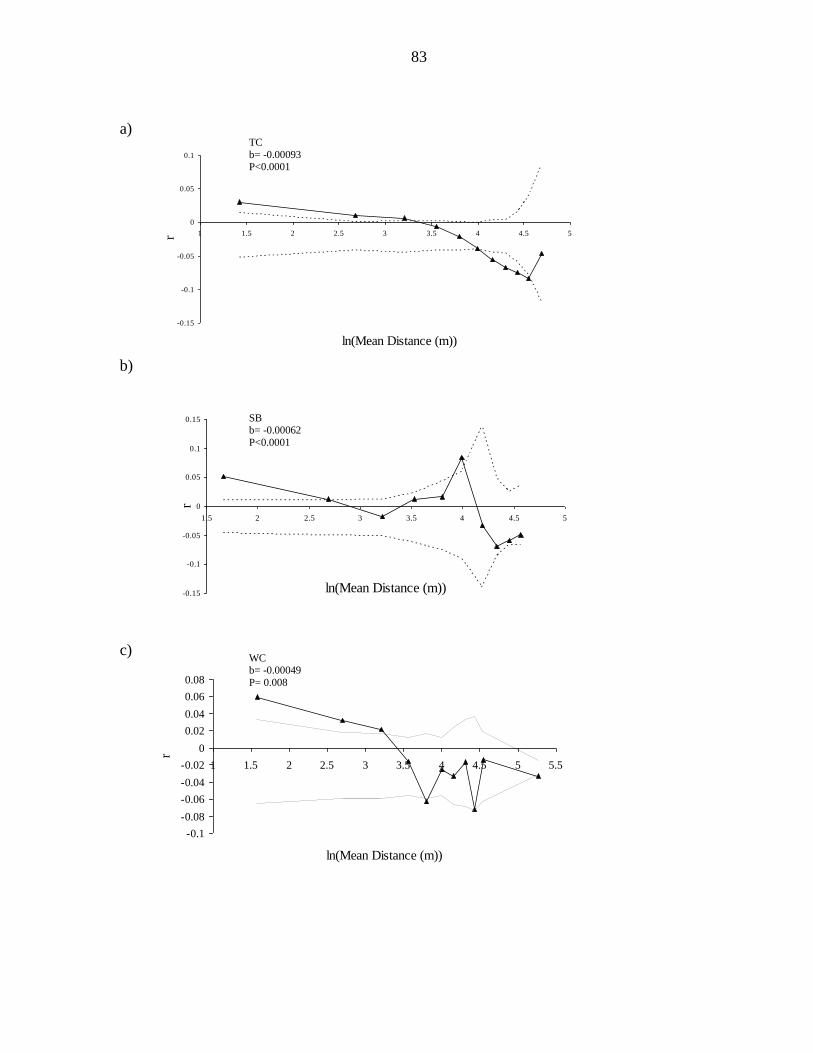
83

a)

b)

c)

-0.15

-0.1

-0.05

0

0.05

0.1

1 1.5 2 2.5 3 3.5 4 4.5 5

ln(Mean Distance (m))

r

-0.15

-0.1

-0.05

0

0.05

0.1

0.15

1.5 2 2.5 3 3.5 4 4.5 5

ln(Mean Distance (m))

r

-0.1

-0.08

-0.06

-0.04

-0.02

0

0.02

0.04

0.06

0.08

1 1.5 2 2.5 3 3.5 4 4.5 5 5.5

ln(Mean Distance (m))

r

WC b= -0.00049

P= 0.008

SB b= -0.00062

P<0.0001

TC

b= -0.00093 P<0.0001

84

d)

e)

Figure 4. Spatial autocorrelation analyses in GenAlEx (Peakall and Smouse 2006) for r statistic

(genetic correlation coefficient averaged over 10 SSR loci) in populations (TC, WC, SB, and 96) for

G. davidsonii. Continuous dashed lines represent the upper and lower bounds of the 95% confidence

intervals around the null hypothesis of r = 0. The mean r is plotted for each distance interval (the

mean distance within a distance class). Also shown are slopes (b) and significance level (P) for a line

fitting r for each population. We also show the overall spatial autocorrelation (e) across all 4

populations using the Heterogeneity test of r produced in GenAlEx (Peakall and Smouse 2006).

Shown is the correlation coefficient of genetic relatedness over 10 meter distance intervals with

dashed lines representing 95% confidence intervals around the null hypothesis (r = 0) and around

each estimate of r.

-0.4

-0.3

-0.2

-0.1

0

0.1

0.2

0.3

0.4

2 2.5 3 3.5 4 4.5 5 5.5 6 6.5 7

Mean Distance (m)

r

-0.150

-0.100

-0.050

0.000

0.050

0.100

0.150

0.200

10 20 30 40 50 60 70 80 90 100

Distance (m)

r

Mean Distance (m)

r

96 b=-0.00013

P= 0.340

ln(Mean Distance (m))

85

Table 1. Description of 10 microsatellite primer sets screened in G. davidsonii. Locus names

are consistent with those given in the Cotton Marker Database, though for convenience, we

have assigned Locus IDs of GD1-GD10. Markers are all published in the Cotton Marker

Database (cottonmarker.org). Shown are forward (PF) and reverse (PR) sequences, fragment

length range (bp), repeat motif and P, the proportion of samples that failed to amplify (in two

attempts).

Locus

ID

Locus

Name

Primer (5'- 3') TA Fragment

Length

Repeat

Motif

P

GD1 DPL0262 PF: TTCTCCATCTCTATCGACTTCCTC 50 130-148 (ATG)13 0.005

PR: TGTCCGTCTTCAAGTTGTCACTAA

GD2 DPL0529 PF: ACTCTCAGGATCTGAGTACAACCC 50 176-200 (CATA)7 0.029

PR: GTTAAAGGATCCTAGTGCTCATGG

GD3 DPL0242 PF: CTTCAGAATTTGGTTCCTGTCTCT 50 224-242 (ATC)7 0.02

PR: AATATAAGGATGTAGCTGATGCCG

GD4 DPL0511 PF: TACATGCAGTGCTACAGAAGAACA 50 167-183 (ATGT)7 0.258

PR: CTTGTATGCCATCATTAACCCTTC

GD5 DPL0513 PF: AGACCCGGCTACTACATGTTATCTT 50 184-200 (GTAT)21

0.029

PR: ACATACAGATGCTTCACACAAACAC

GD6 DPL0541 PF: GAAATGCTTGTGGGAACTGAAT 50 224-244 (TATG)1

1

0.083

PR: GCTTCCTCCCTTACAATCAAATCT

GD7 MUCS094 PF: CTAAACAAGAGTCGTTGGAGCC 50 167-191 AAC(2)A

GC(5)

0.044

PR: AGCATCTCATCTTTCTTTTCGC

GD8 Gh537 PF: GTTGGGTGGCAATTCCTTTTAGATC 50 197-221 AGA(8) 0.049

PR: AAAGCTAATCCCTATACCTTTTCTTC

G

GD9 MUSS530 PF: CGTAGCCGTTCAGTTTCTCC 50 246-270 AG(8) 0.049

PR: AAACCAAATCCAGAGAGAAGG

GD10 MUCS586 PF: ATCCAGCCAAACCAAAAGC 50 370-394 TTGG(2)

CTG(3)

0.107

PR: TTCCAATGCATAGCGAAGG

86

Table 2. Results from the multiple regressions on distance matrices, with dependent variables of Seed and Leaf

damage and pairwise distance matrices of independent variables of Genetic Distance (GD), Geographic

Distance (GGD), Trichome Density Dissimilarity (Trich), Seed Gland (Lysigenous Cavity) Dissimilarity (SdGl),

and Leaf Gland (Lysigenous Cavity) dissimilarity (LGl). Leaf Damage dissimilarity or Seed Damage

dissimilarity were included in the model in which the term was not assigned to the role of a response variable.

Shown are four populations of G. davidsonii, Coefficients of regression for each independent variable on the

tested response, P-value of that coefficient, R2 for the complete model for each response x population

combination, and the proportional effect size of each independent variable of the complete model (all identified

effects) using a proportion of the R2 and by use from ANOVA.

Population

Response

Variable Effect Matrix Coefficient P

complete

model R2 Effect Size (R2) Effect Size (ANOVA)

TC Seed Damage GD 0.00058 0.627 0.0123 0.0148

GGD 0.00079 0.035 0.2125 0.2555

Trich 0.00155 0.034 0.2666 0.3205

SdGl -0.00114 0.621 0.0196 0.0236

LDam 0.151 0.102 0.1407 0.1692

LGl 0.00216 0.061 0.1800 0.2164

0.017 0.0353

Leaf Damage GD 1.69E-03 0.001 0.4819 0.5786

GGD -6.17E-05 0.697 0.0059 0.0071

Trich 1.17E-04 0.712 0.0069 0.0082

SdGl 9.89E-04 0.287 0.0677 0.0813

SdDam1 3.37E-02 0.099 0.1436 0.1724

LGl 8.50E-04 0.057 0.1269 0.1524

0.001 0.0346

WC Seed Damage GD 0.00032748 0.625 0.0065 0.0063

GGD 5.39E-05 0.099 0.0552 0.0537

Trich 0.000404196 0.297 0.0424 0.0412

SdGl 0.00170044 0.058 0.1259 0.1225

LDam 0.289925476 0.001 0.6462 0.6283

LGl -0.0008893 0.099 0.1522 0.1480

0.001 0.0411

Leaf Damage GD -1.82E-05 0.956 0.0000 0.0000

GGD -2.42E-05 0.238 0.0300 0.0326

Trich -1.74E-04 0.511 0.0211 0.0230

SdGl 1.60E-03 0.011 0.3056 0.3327

SdDam 9.30E-02 0.001 0.5603 0.6099

LGl -5.50E-05 0.890 0.0016 0.0017

0.010 0.0471

SB Seed Damage GD -6.29E-04 0.430 0.0082 0.0103

GGD 8.95E-06 0.171 0.0454 0.0568

Trich 3.33E-04 0.412 0.0099 0.0123

SdGl 5.01E-03 0.001 0.4589 0.5737

LDam 3.43E-01 0.002 0.1557 0.1947

LGl 1.40E-03 0.006 0.1218 0.1522

0.001 0.1063

Leaf Damage GD -7.59E-04 0.017 0.2525 0.2976

GGD -1.09E-06 0.660 0.0141 0.0166

Trich -7.07E-05 0.669 0.0093 0.0109

SdGl 4.26E-04 0.320 0.0661 0.0779

SdDam 5.31E-02 0.002 0.5038 0.5936

LGl -4.79E-05 0.816 0.0029 0.0034

0.018 0.0355

96 Seed Damage GD 8.24E-05 0.922 0.0002 0.0002

GGD 8.25E-07 0.744 0.0019 0.0020

Trich 3.32E-03 0.001 0.8652 0.8740

SdGl -1.45E-04 0.885 0.0006 0.0006

LDam 1.31E-01 0.114 0.0809 0.0817

LGl 1.23E-03 0.224 0.0412 0.0416

0.002 0.0616

Leaf Damage GD -1.35E-04 0.790 0.0030 0.0031

GGD -6.13E-06 0.003 0.7702 0.8049

Trich 1.45E-05 0.968 0.0001 0.0001

SdGl 1.61E-05 0.99 0.0000 0.0000

SdDam 4.04E-02 0.101 0.1746 0.1825

LGl 2.17E-04 0.772 0.0088 0.0092

0.116 0.0295

87

Supplementary Information

Figure S1. Spatial autocorrelation of leaf gland (lysigenous cavity) density over geographic

distance (in meters) within site SB. Shown is the correlation coefficient (r) of leaf gland

density dissimilarity among plants within geographic distance classes of 25 m. Indicated is an

estimate of the phenotypic correlation (solid line) + 95% confidence interval (bars) around

the estimate as well as 95% confidence intervals around the null hypothesis of no correlation,

dotted lines (r = 0).

Figure S2. Spatial autocorrelation of trichome density over genetic distance within site SB.

Shown is the correlation coefficient (r) of trichome density among plants within genetic

distance classes (genetic similarity). Indicated is an estimate of the phenotypic correlation

(solid line) + 95% confidence interval (bars) around the estimate as well as 95% confidence

intervals around the null hypothesis of no correlation, dotted lines (r = 0).

-3.000-2.000-1.0000.0001.0002.0003.0004.0005.0006.000

25 50 75 100

Geographic distance (m)

r

-2.000

-1.000

0.000

1.000

2.000

3.000

9.5 19 28.5 38

Genetic Distance

r

88

Table S1.Ten Simple Sequence Repeat (SSR) loci used for population analyses of G.

davidsonii. Shown are abbreviated names (GD ID), names identified on the Cotton Marker

Database, repeat motif of the SSR, number of samples amplified per locus (N), number of

alleles (Na), Allelic Richness (AR), Observed and expected heterozygosity (HO and HE) and

Weir and Cockerham’s (1984) FST and FIS. Bolded mean FST and FIS estimates are highly

significant (P<0.001).

GD ID Name Repeat Motif N Na HO HE FST FIS

GD1 DPL0262 (ATG)13 202 7

0.39

0.734 0.032 0.482

GD2 DPL0529 (CATA)7 197 7

0.238

0.642 0.083 0.635

GD3 DPL0242 (ATC)7 199 7

0.278

0.658 0.075 0.586

GD4 DPL0511 (ATGT)7 150 5

0.492

0.566 0.092 0.07

GD5 DPL0513 (GTAT)21 197 5

0.145

0.549 0.138 0.743

GD6 DPL0541 (TATG)11 186 6

0.188

0.593 0.08 0.681

GD7 MUCS094 AAC(2)AGC(5) 194 9

0.15

0.436 0.009 0.667

GD8 Gh537 AGA(8) 193 10

0.349

0.729 0.072 0.533

GD9

MUSS530 AG(8) 193 13

0.277

0.571 0.017 0.532

GD10 MUCS586 TTGG(2)CTG(3) 181 17

0.411

0.723 -0.003 0.46

Mean --- 189 9 0.292 0.620 0.06 0.535

89

Table S2. Locus-specific measures of genetic diversity within 4 populations of G. davidsonii.

N= population sample size, NA = number of alleles, HO = observed heterozygosity, HE =

expected heterozygosity for each population.

Locus TC WC SB 96

ID N NA HO HE

N NA HO HE

N NA HO HE

N NA HO HE

GD1 49 5 0.367 0.738 49 6 0.469 0.77 49 6 0.367 0.691 55 7 0.345 0.738 GD2 49 4 0.122 0.653 48 6 0.229 0.679 49 4 0.286 0.595 51 6 0.314 0.642 GD3 49 5 0.245 0.718 47 5 0.383 0.711 49 5 0.224 0.538 64 6 0.259 0.664

GD4 42 3 0.548 0.487 41 3 0.683 0.565 43 3 0.488 0.523 30 5 0.250 0.690

GD5 48 5 0.146 0.566 48 4 0.104 0.675 48 4 0.271 0.58 53 5 0.057 0.373 GD6 44 6 0.205 0.565 43 5 0.163 0.664 44 5 0.114 0.522 55 5 0.273 0.629 GD7 45 8 0.133 0.402 48 4 0.188 0.311 48 6 0.208 0.57 53 4 0.075 0.477

GD8 45 8 0.444 0.641 48 7 0.333 0.726 47 9 0.34 0.73 53 9 0.283 0.815

GD9 45 12 0.356 0.578 47 8 0.298 0.519 48 10 0.271 0.471 53 10 0.189 0.724 GD10

44 13 0.5 0.767 46 10 0.478 0.728 39 7 0.333 0.759 52 10 0.327 0.731

90

CHAPTER 4. Comparison of quantitative defense traits and genetics in determining

evolution of defense syndromes in a wild Sonoran Desert cotton endemic, Gossypium

davidsonii

A paper to be submitted to The American Journal of Botany

Adam Kuester and John Nason

Abstract

Gossypium davidsonii, a wild cotton species endemic to the Sonoran Desert in Baja

California, has been characterized as possessing multi-fold variation in defense traits,

including glanded phenotypes in leaf and seed material as well as foliar trichome density,

within and among natural populations. Causes of trait variation have yet to be determined.

We estimated genetic differentiation among populations using neutral genetic markers, FST,

and an analogous phenotypic statistic for differentiation among wild populations, PST, to

determine the level and direction of selection on defense traits in 21 populations. While we

find a high level of genetic differentiation among populations (FST = 0.182), we similarly find

high levels of differentiation in the observed phenotypes (PST trichome = 0.312, PST Leaf

lysigenous cavity = 0.570, PST Seed lysigenous cavity = 0.644), which suggest divergent

selection across the range of G. davidsonii. We interpret this pattern as being driven by

differences in insect herbivore communities on the cotton host across the species’ range.

Key Words: PST; FST; Gossypium davidsonii; trichome; gossypol; lysigenous cavity

91

Introduction

Phenotypic variation can be a result of several factors, of which environment and

genetic components are often two common contributors (Falconer and Mackay, 1996).

Consequently, both intra and inter-population variation can be important parts of quantitative

trait variation within a species. In fact, intra-organismal phenotypic variation can result from

acclimatization to changing environments, such as seasonal climate variation (Clarke, 1993),

behavioral polymorphism resulting from changing predation pressure (Wilson et al., 1993),

learned behaviors from changing food sources (Lewis and Takasu, 1990), and other

disturbances (Gates and Edmunds, 1999). Phenotypic plasticity, the result of a certain

genotype producing different phenotypes under varying environmental conditions, has also

been identified as a means of accelerating the process of adaptive evolution in allowing

populations to become established (Ghalambor et al., 2007; West-Eberhard, 2003), especially

favoring situations when the level of environmental heterogeneity is smaller than that of an

organism’s dispersal capabilities (Baythavong and Stanton, 2010).

Plastic responses to environmental stimuli are quite common in non-motile terrestrial

plants (Schlichting, 1986) as a means to efficiently utilize resources (Schlichting, 1986;

Jackson and Caldwell 1996; Pintado et al. 1997) and redirect them for plant defense

(Agrawal, 2001). The study of intra-organismal variation in plant traits has traversed many

morphological and physiological aspects of plant responses to the environment, such as light

environments on leaf morphology (Talbert and Holch, 1957; Jurik, 1986), defense responses

to herbivores and pathogens (Zangerl et al., 2002; Xu et al., 2004; Townsend et al., 2005),

responses from mowing (McNaughton, 1983), and competition (Casper and Jackson, 1997;

92

Aerts, 1999), which all have been decidedly well-defined plastic responses. Plastic traits have

a substantial environmental effect (E) component affecting trait expression.

Despite many examples of plasticity in nature, spanning taxa and responses to

environmental effects, variation in traits is not always a result of the environment in which an

organism lives. Individuals may be genetically-wired for specific phenotypes. The degree to

which trait variation is influenced by the genetics of an individual can often vary

substantially across traits. Under circumstances of purely genetic influence, variation

primarily results from mutations in genes involved in the expression of a phenotype, whereby

more phenotypic variation is largely a result of the degree of non-silent mutations in genes,

representing a genetic effect (G) on an individual’s phenotype.

Often, heritability does not account for all of the phenotypic variation in a population.

Rather, a more realistic circumstance of phenotypic variation results from a combination of

environmental influence on genetic expression of a trait, a genetics-by-environment (GxE)

effect within a species or population, whereby genotypes respond dissimilarly to differing

environmental conditions. Variation in phenotype within and among populations may be a

product of either or G, E, or GXE effects, but is likely from a combination of all these effects.

When a trait has a strong vertical transmission, natural trait variation in populations

may be greatly influenced by natural selection or from the stochastic processes of genetic

drift. Phenotypic trait variation in a species may reflect different local optima for a trait,

where a different phenotype is adaptive in different local populations (divergent selection).

Alternatively, reduced variation within species may represent a global optimum in the trait

across all populations (stabilizing selection). On the other hand, observed variation may

reflect similarities to variation in neutral genetic signals or mutation-drift equilibrium.

93

By comparing phenotypic differentiation of quantitative genetically-inherited traits

among populations, QST, to genetic differentiation among populations derived from neutral

genetic markers, FST, one can also estimate the degree to which natural selection is acting on

a trait (Andrew et al., 2005; Evanno, 2006; Martin et al., 2008). A significant FST statistic

reflects genetic differentiation among populations as a result of genetic drift, mutation, and

migration. QST, on the other hand, measures a quantitative trait that may have been

influenced by natural selection or by stochastic processes. As we expect that our estimation

of FST is from genetic markers that are not under selection, FST can be used as a null model

against which to determine the strength and direction of selection on specific phenotypes. As

QST is intended to measure the among-population total additive genetic variance of a

quantitative trait, it is typically quantified from individuals across populations grown in a

common garden setting, so as to minimize contribution of variation due to environment and

non-additive effects on the observed phenotype.

Though common garden experiments may be ideal in determining the direction and

strength of selection in domesticated species and recommended for the study of QST

(Whitlock and Guillaume, 2009), such experiments have often been impractical or may

portray a biased estimate of quantitative traits from unrealistic environmental conditions,

resulting in a severe GxE interaction (Saether et al., 2007). With additional a priori

knowledge of inheritance patterns or of the effects of environment and inbreeding (effects

that can often distort measurements of pure additive genetic traits), it can still be possible to

assess the extent to which phenotypic traits are under natural selection (Ritland, 1986;

Andrew et al., 2005). In truth, if one could rule out non-additive genetic effects and the

environment as playing large roles in phenotype variation, then measurements of phenotypic

94

differentiation from natural populations (commonly referred to as PST or Psuedo-QST) may be

more realistic than a measurement of QST from a glasshouse environment. An informed PST

estimate, thus, should at least approximate one of QST, having considered the delicateness of

certain assumptions made. The comparison of QST or PST to FST can indirectly determine

whether, and the extent to which, natural selection is acting on a trait within a species.

Plants have evolved many mechanisms by which to cope in complex environments to

stresses of insect herbivores and pathogens, in addition to other environmental conditions.

Understanding the evolutionary mechanisms behind plant defense can be very important in

determining how plant populations have evolved to cope with insect herbivore pressures.

Gossypium davidsonii, a wild cotton species endemic to the Sonoran Desert, displays

variation in seed (8-fold, Stipanovic et al., 2003) and leaf (10-fold, Kuester and Nason, in

prep) gossypol expression. Additionally, Phillips and Clements (1967), when originally

documenting the species’ range, observed marked variation in several phenological

characteristics. Kuester and Nason (in prep) found that there was no profound effect from

extreme herbivory, nutrients, water, or interacting terms on defense trait expression in G.

davidsonii. In fact, often the largest proportion of the variation was caused by population-

level differences in plant traits. Environmental effects on defense traits were negligible in

leaf tissue (Kuester and Nason, in prep) and seed glanded phenotypes (Bell and Stipanovic,

1977). Therefore, variation in the wild should be primarily due to genetic differentiation

within and among populations.

The objectives herein are to address the potential mechanism for marked phenotypic

variation in defense traits within the species G. davidsonii by means of an informed PST - FST

analysis. We will gain insightful information as to whether variation in defense traits in G.

95

davidsonii, and more broadly in the genus, results from selection or is a mere artifact of

genetic drift. This information will lead to further ecological questions as to how defenses are

utilized within the species and the degree to which different defense strategies are favored

across populations and to which a heterogenic defense landscape has necessitated the

evolution of divergent defense phenotypes within the species.

Materials and Methods

Study Sites- Populations of Gossypium davidsonii were identified in the southern,

Cape Region of the Baja California peninsula, Mexico. A drought-deciduous shrub, G.

davidsonii grows in response to summer rains (July-September) with leaves and flowers

persisting until December-January. In total 21 populations were identified and used in this

study. Population sizes for phenotypic and genotypic sampling and coordinates are provided

in Table 1. Each site location was recorded with GPS. The region and the site positions of all

sites are described in Figure 1.

Plant Material- Four fully expanded healthy leaves, randomly collected from each

plant, were dried whole in silica gel for preservation and then later stored at -80 °C for

phenotypic analyses. One expanding leaf was selected per individual and stored in silica gel

at -80 °C until use for genetic analysis. In most cases, at least 15 plants were selected per

population. In one case (site 141), where plants were scarce, fewer than 15 plants were used

(Table 1).

Seeds from at least 3 fruits per plant were also collected. Seeds from individual fruits

were packaged separately in coin-envelopes. All seeds were inspected by the Secretaria de

96

Ganaderia Agricultura Rural Pesca y Alimentacion (SEGARPA) prior to importation to the

United States. Permit by the USDA, PPQ 562, permitted importation of cotton seed.

Isolation of DNA-Fifteen milligrams of silica-dried leaf material was used for DNA

isolation. The leaf tissue was ground using the Genogrinder 2000, then extracted using the

Autogen Autogenprep 740 DNA extraction robot at the Iowa State University DNA Facility.

All DNA samples were eluted in water. Concentration of DNA was determined by

spectrophotometry and dilutions of 20 ng/ μl were prepared for use in Polymerase Chain

Reactions (PCR).

SSR loci- Of 50 Simple Sequence Repeat (SSR) loci screened from the Microsatellite

Database, as previously described in Kuester and Nason (2012) (Table S1, Supplementary

Information), six (GD1-GD6) were identified as being polymorphic in G. davidsonii for use

in this study Table 2). Forward primers were attached to an M13 tag, used for cost-effective

fluorescent allele calling (Schuelke, 2000). A mixture of the sense primer and labeled M13

tagged primer were combined in a ratio of 15 labeled M13 primer: 1 forward primer. All

primers were obtained from Integrated DNA Technologies (Corralville, IA). Though recent

work has advised against using SSR loci for estimating FST to which to compare QST, as

mutation rates in microsatellite loci are often high and not reflective of a simple evolutionary

mode (Edelar et al. 2011), we believe the use of microsatellite loci within our system is

warranted, as polymorphism within loci is low (pers. obs.) and other marker-based loci have

proved ineffective at detecting genetic variation within the species (Wendel and Percival,

1990).

97

These 6 SSR loci were split into two multiplexes, as fragment size overlap

constrained running all loci together in one reaction. Description of multiplexing procedure

and conditions for PCR has been described in Kuester and Nason (2012).

One μl of PCR product was used for fragment detection using an Applied Biosystems

3730 DNA Analyzer (Carlsbad, CA) at the Iowa State University DNA Facility. An ABI

GS500 size standard was used for fragment length comparison. All samples were analyzed

using Applied Biosystems (Carlsbad, CA) PeakScanner 1.0 analytical software. A PP (Primer

Peaks adjustment) sizing default was used for the analysis. Front peaks were scored as the

true allele on occasion where stutter was noticeable from PCR reaction.

` Phenotypic data- Seed gossypol levels were quantified by counts of lysigenous cavity

density in longitudinal sections. Gossypol concentration measured by HPLC consistently

correlates across species with visual inspection of lysigenous cavity density in sections of

cotton seed (Benbouza et al., 2002). The average cavity count of 3 seeds was taken from each

of 3 fruits per plant that were selected from each plant in 21 populations of G. davidsonii.

The largest seed from each fruit were chosen. Seeds were cut longitudinally and filmed at

2.5X magnification with a Nikon CoolPix 4500 (Tokyo, Japan) camera under an Olympus

SZ61 (Center Valley, PA) microscope. Lysigenous cavity counts per one half seed section

were standardized to surface area of the section. We report seed cavity density as number of

cavities per mm2. Surface areas were calculated with Image J (Rasband 2002-2009).

We quantified trichomes from leaf material dried in silica gel under 2.5 X

magnification with an Olympus SZ61 (Center Valley, PA) microscope. Silica gel

preservation of leaf material caused no apparent damage to leaf trichomes (pers. obs.). Three

samples from 3 separate leaves were counted in order to estimate an average leaf trichome

98

density per plant (# trichomes per mm2). Each sampled plant per population was quantified.

Quality of leaf material created difficulty quantifying leaf lysigenous cavity density for site

160. Seed was not collected from two sampled populations (19.2 and 141).

Data Analysis

Genetic Diversity- We used MicroChecker (Van Oosterhout et al., 2004) to evaluate

our scoring of microsatellite genotypes and test for potential scoring errors resulting from

stuttering, large allele drop out, and null alleles. Since we suspect G. davidsonii of being a

selfing species, we anticipated excess homozygosity within populations at all loci, ultimately

deviating from Hardy-Weinberg Equilibrium (HWE). Because null alleles cannot be directly

inferred by MicroChecker, we quantified the number of individuals for which we were

unable to amplify a given locus after at least two attempts as indicating proportion of

homozygous null alleles. Loci that amplified were independently scored twice to check for

scoring accuracy and we recorded the scoring error rate for each locus within the species.

All SSR loci in each population of G. davidsonii were tested for HWE using the

Hardy Weinberg Exact Tests in Genepop on the Web (Raymond and Rousset, 1995; Rousset,

2008), using the probability test (sub-option 3). Microsatellite loci were also tested for

linkage disequilibrium (LD) using Fisher’s method for multiple probabilities for each pair of

loci across population using the genotypic linkage disequilibrium test in Genepop. Since

multiple significance tests were performed in detecting LD and HWE, a sequential

Bonferroni correction (Rice, 1989) was used to determine significant deviation.

Number of alleles, allelic richness, and observed and expected heterozygosity were

all assessed using FSTAT version 2.9.3 (Goudet, 2001).

99

We employed the use of Wright’s F-statistics (Wright, 1965) to determine the degree

of population structuring in our datasets. We estimated FIS, a measure of inbreeding of the

individual relative to the population and of deviation from random mating and FST, a metric

of genetic differentiation among populations, using Weir and Cockerham (1984)

implemented in FSTAT.

RST was also calculated to determine whether a step-wise mutation model best

represented our data sets. Because FST was not significantly different from RST with 1000

permutations of RST (pRST), we assume an infinite alleles model. We, thus, only report

estimates of FST, since it has lower variance than RST (Hardy et al., 2003).

We accounted for suspected null alleles indicated by Microchecker by estimating FST

with the program FreeNA (Chapuis and Estoup, 2007) to compare FST adjusted for null

alleles (excluding null alleles) and FST assuming no null alleles. As both estimates produced

similar results (Table S1, Supplemental Information), we report only FST not adjusted for null

alleles. Since Edelar et al. (2011) suggest that microsatellite loci might be problematic in

estimating FST for an FST-QST comparison due to high mutation rates, we ran a preliminary

comparison of the effect of number of alleles per locus on the estimate of FST and Hedrick’s

(2005) maximum FST adjusted for allelic richness. After pooling rare alleles so that only two

alleles per locus remained, we found that the Weir and Cockerham’s (1984) FST decreased

only by 0.02 (about 10% of the FST estimate), leading us to believe that the examined loci

were appropriate for use in an FST-QST context. We also heeded Edelar et al.’s (2011) advice

to use an AMOVA-based ΦST calculation for comparison, as distance-based calculations of

FST are not affected by mutation rates. Upon calculating ΦST in GenAlEx (Peakall and

Smouse, 2006), we noted little difference between the AMOVA-based estimate and one

100

estimated by the Weir and Cockerham (1984) method and thus will only present the latter

estimate of FST.

Isolation by Distance-Isolation by distance was tested by regressing population pair-

wise estimates of linearized FST (FST/(1- FST); Rousset, 2000) on the natural log of inter-

population geographic distance using the Mantel test implemented in ISOLDE option of

Genepop. We compared two geographic distance models: (1) the Euclidean distance between

populations and (2) a distance that takes into account the Sierra de la Laguna mountain range,

which runs through the Cape Region, as a potential barrier to gene flow. For populations

separated by this mountain range, we calculated distances through a point either at the

southern end of the peninsula where the mountains end (N 22.9795°, W 109.8846°) and

northern extent to the mountains (N 23.920347°, W 110.264952°), selecting the shortest path.

The preferred geographical distance model was selected as having a lower p-value and a

higher coefficient of determination (R2). We similarly compared Cavalli-Sforza chord

distance and conditional genetic distance (cGD) on spatial distance, as these alternative

genetic distance metrics may be more powerful than linearized FST (Takezaki and Nei, 1996;

Dyer et al., 2010). We only report the genetic distance metric that provides the clearest

signature of isolation by distance (by comparing R2 and p-values among the three distance

metrics). We also explored if the Sierra de la Laguna Mountains were a barrier to gene flow

by running a hierarchical AMOVA to estimate FST between sites east and west of the

mountain range in Arlequin (Excoffier et al., 2005). We ran an additional hierarchical

AMOVA to determine the degree to which cotton within the southern portion of the species’

range (hosting the boll weevil) was genetically structured from that of cotton in the rest of the

range.

101

PST Calculation for inbred organisms- Selection on quantitative traits can be

discerned by comparing phenotypic differentiation to genetic differentiation found by neutral

molecular markers. We calculated quantitative trait differentiation for each of the three

evaluated phenotypic traits as:

PST = Vbetween

Vbetween +2Vwithin

where Vbetween and Vwithin are phenotypic variance components among and within populations,

respectively. The variance components were identified from ANOVA of the phenotypic data

for each trait across populations in JMP v. 8.0.2.

PST is assumed to be calculated from additive phenotypic traits, thus inbreeding can

inflate the estimate (Bonnin et al., 1996). Because we suspect that G. davidsonii inbreeds, we

adjusted for inbreeding (Equation 9 of Bonin et al., 1996) by multiplying 1+FIS (Weir and

Cockerham’s (1984) inbreeding coefficient) to the between-population variance component.

We assessed a possible correlation between seed and fruit lysigenous cavity densities

by using collections from field and glasshouse plants. This analysis determined whether seed

lysigenous cavity densities measured across populations was a good indication of lysigenous

cavity density phenotypes within the fruit at the time insect herbivore specialists oviposit and

develop inside. We quantified the lysigenous cavity density per mm2

area averaged from each

of 3 locule walls per capsule and 3 seeds per fruit (one seed each from 3 locules per capsule).

Seed and fruit lysigenous cavity density were quantified as described above for lysigenous

cavity density phenotypes. As we found a significant and positive correlation between fruit

and seed lysigenous cavity density (R2

= 0.389, P < 0.001), we will only measure the

102

lysigenous cavity density of field collected seed as a proxy measurement of lysigenous cavity

density within fruits.

PST - FST comparison- To understand how different defense traits in G. davidsonii

have been evolving, we use a PST – FST comparison. Since contemporary methods to estimate

variance around PST rely on a large number of populations (Gay et al., 2009), we used a 95%

confidence interval estimate from the Lewontin and Krakauer (1973) distribution of FST for a

two-tailed test to determine whether PST significantly diverged (Whitlock, 2008). Since our

FST estimate was from presumably neutral markers, we used this estimate as our null

evolutionary model; a statistically greater value of PST will be interpreted as evidence of

divergent selection among populations arising as a result of directional selection for

alternative trait values in different populations stabilizing selection for different adaptive

optima in different populations, and a statistically smaller value will reflect stabilizing

selection. Since PST estimates are sensitive to un-quantified environmental and non-additive

genetic effects (Pujol et al., 2008), these estimates must be interpreted cautiously (Brommer,

2011). We determined in previous work that the effect of extreme environmental conditions

commonly impacting plant defense was minimal (less than 20% in defenses) and cannot

explain several-fold variation in defense phenotypes across G. davidsonii’s species range

(Kuester and Nason, in prep).

We tested the effects of genetic differentiation (as measured by FST), geographic

distance, and presence or absence of boll weevils within G. davidsonii populations on PST for

each measured trait to test their relative effects on defense phenotypes in these wild cotton

populations. We utilized multiple regressions on distance matrices (MRM) in the Ecodist

package (Goslee and Urban, 2007) in R (R Development Core Team, 2005). We also used

103

MRM to assess pair-wise trade-offs in defense traits between each individual plant per

population, taking into account genetic distance (Cavalli Sforza distance), ln(geographic

distance), and presence or absence of boll weevil. Defense trait trade-offs, using population

averages, were similarly assessed.

Results

Genetic Diversity- Levels of large allele drop out, stutter, null alleles, and % missing

genotypes can be found in Table S2. Across loci, we found a scoring error rate of 2.8% after

double scoring genotypes.

All but 4 populations deviated from HWE: 19.2 (P = 0.004), 165 (P = 0.019), SB (P =

0.0327), and 96 (P = 0.0192) (Table S3, Supplemental Information). With the exception of

GD4, where only 5 of 21 populations deviated from HWE, all other loci exhibited deviations

from HWE in at least half of sampled populations. The HWE assumption of nonrandom

mating appeared to be violated, as inbreeding coefficients for these five loci indicated high

and significant levels of inbreeding. Estimates of FIS over all loci for each population ranged

from 0.125 to 0.789 (mean = 0.431, Table S3, Supplemental Information).

For each locus pair across populations within G. davidsonii, there were 3 of 15 pairs

that were in linkage disequilibrium: GD1 and GD2 (2=68.8, P = 0.003), GD1 and GD3

(2=66.17, P = 0.006), GD2 and GD3 (2

=77.89, P < 0.001).

Relatively low levels of SSR genetic diversity were observed in the G. davidsonii loci,

with ranges in allelic diversity from 5-8 alleles per locus, gene diversity from 0.32-0.56

(mean= 0.477, Table 2), and allelic diversity from 1.27- 1.53 (mean = 1.44, Table 2).

104

We observed high levels of genetic differentiation among the cotton populations, with

mean FST = 0.182 (P < 0.001, 95% confidence interval = 0.087, 0.311). All loci produced

significant FST estimates (P < 0.010). Of the six loci, four yielded similar results around the

mean, though GD4 had FST = 0.066. Since re-estimating the global FST excluding GD4

produced a similar result (FST = 0.201, P < 0.001), we report the estimate including GD4.

We identified 10 populations of G. davidsonii where boll weevil was present and 11

sites where no boll weevils were found (Table 1). In observing populations hosting boll

weevils separate from other populations, we detect a much lower FST than found when

analyzing all populations together (FST = 0.120, P < 0.001 ; Table 3). Sites with no apparent

boll weevil activity, on the other hand, have a substantially larger (P = 0.057) FST of 0.239, P

< 0.001.

Inbreeding coefficients, FIS, for each of these loci ranged between 0.41 and 0.66,

which may indicate high levels of inbreeding, though GD4 produced FIS = -0.02 (Table 2).

All FIS estimates but that produced from GD4 were significantly different from 0.

Isolation by Distance-We found no large pattern of isolation by distance, given the

large differentiation among populations (Figure 2 a and b), neither using isolation by

Euclidean distance nor by distances connected around the Sierra la Laguna mountain range

through the center of the Baja Peninsula. Cavalli-Sforza chord distance explained more

variation in the data set and produced more significant results than linearized FST or

conditional graphical distances. Since there was little evidence of plants inhabiting areas

within the central mountain range of the peninsula, we suspected the mountains as a potential

geographic barrier to gene flow.

105

We noticed no effect of the mountain range on regional genetic structuring within G.

davidsonii (FRT = 0.000, P = 0.360). We found a small effect of regional structure between

boll weevil and non-boll weevil hosted cotton populations (FRT = 0.030, P = 0.005).

Quantitative Trait variation- We detected similar ranges for leaf lysigenous cavity

and gossypol levels between USDA accessions and field-collected specimen, but saw more

restricted phenotypic ranges in USDA accessions for seed lysigenous cavity and leaf

trichome levels, though ranges overlap (Table 4). All traits quantified from field-collected

material revealed that population was a high contributor to variation with each trait in

ANOVA (Table S4, Supplementary Information). All three PST estimates were significantly

larger than that of FST. We noticed that inclusion of inbreeding deflated PST estimates for all

traits, but estimates nonetheless remained significantly greater than the estimate of FST.

We detected nearly 3.5-fold variation in leaf gossypol concentrations, 3-fold variation

in seed lysigenous cavity density, and 2-fold variation in leaf and trichome density across G.

davidsonii populations (Table 4).

In assessing tradeoffs between defense traits, we found that trichome and seed (r = -

0.181, P = 0.057) and leaf (r= -0.040, P = 0.001) lysigenous cavity and between leaf and seed

lysigenous cavity densities(r = -0.301, P = 0.005) were all negatively correlated.

The estimates for PST over all sites were greater than those among only boll weevil-

infested sites for leaf and seed lysigenous cavity density measurements (PST boll weevil leaf

lysigenous cavity = 0.389, PST leaf lysigenous cavity all sites = 0.570; PST seed lysigenous

cavity boll weevil = 0.237, PST seed lysigenous cavity all sites = 0.644). The estimate for leaf

trichome density was smaller than when looking only at sites where boll weevils were

present (PST trichome boll weevil = 0.426, PST trichome all sites = 0.312, Table 5).

106

PST -FST comparison- Of sites where boll weevils were present, PST was significantly

greater than FST for leaf lysigenous cavity and trichome density traits. Of the sites where boll

weevils were not present, PST was significantly larger for leaf trichome and seed lysigenous

cavity traits (Table 5).

PST estimates for each defense phenotype, leaf and seed lysigenous cavities and leaf

pubescence, were significantly larger than our estimate of FST (Figure 3). When looking at

only sites where we observed boll weevils, the PST estimates were reduced, but similarly

large, in comparison to FST over the 10 sites hosting A. grandis populations.

Given variation both within and among populations for each defense trait, we

compared phenotypic distances across populations and correlate this to pair-wise FST

estimates. We only noticed a weak, marginally significant relationship between leaf

lysigenous cavity density and genotype (R2 = 0.011, P = 0.080) and found no trend when

evaluating the other defense traits and genetics (trichome: R2 = 0.003, P = 0.180; seed

lysigenous cavity density: R2 = 0.004, P = 0.270).

Pair-wise comparison of mean phenotypes between populations showed a significant,

though very weak, pattern of isolation by distance for trichome density (R2 = 0.026, P =

0.027), seed lysigenous cavity (R2 = 0.11, P <0.001), leaf lysigenous cavity (R

2 = 0.023, P =

0.027) (Figure 4).

While leaf lysigenous cavity PST appeared to be sensitive to inter and intra-heritability

for leaf trichome and seed lysigenous cavity PST estimates did not seem much affected

(Figure S1a-c, Supplemental Information).

107

We found no effect of boll weevil presence on phenotypic differentiation in defense

traits (leaf lysigenous cavity: r = -0.003, P = 0.935; seed lysigenous cavity: r = -0.0555, P =

0.332; trichome: r = -0.0221, P = 0.662) having taken into account genetic and geographic

distances. The only significant effect we detected was of genetic distance on PST for seed

lysigenous cavity density, having taken into account geography and boll weevil presence (r =

0.523, P = 0.049).

Discussion

Our objective within this study was to determine the source of large variation

observed across the range of G. davidsonii. We found that genetic drift alone is insufficient

to explain the observed differentiation of G. davidsonii’s defense traits. In fact, these traits

are likely under divergent selection among populations, though we have no evidence of the

extent to which the traits defend against insect herbivores. While comparing infested sites to

those without boll weevils, we observed significant differences among populations in

gossypol-related traits, but no signal of stabilizing selection within the boll weevil region.

Likewise, we saw no trend in foliar trichome production within the boll weevil region, nor

did we detect differences in pubescence between infested and un-infested areas.

Lysigenous cavities are important for defense against generalist herbivores in

Gossypium and related genera by producing gossypol and related terpenoids (Stipanovic et

al., 1986; Stipanovic et al., 2003). Gossypol, an important toxic deterrent to many insect

herbivores (Shaver and Parrott, 1970; Meisner et al., 1977; Hedin et al., 1991), is found in

high concentrations within G. davidsonii (Kahn et al., 1999; Stipanovic et al., 2003). The

compound has also been identified as an attractant for boll weevil oviposition and as a

108

possible precursory agent used to enhance boll weevil aggregation pheromone (Hedin and

McCarty, 1995). If boll weevils were a selective force on glanded phenotypes, we would

expect to observe selection for lower levels of gossypol in areas of boll weevil presence, but

find no difference in gossypol traits, after accounting for genetic and geographic distances

between sites with and without the insect.

We, likewise, found no difference in leaf trichome densities between sites with and

without boll weevils, upon accounting for geographic and genetic differences. Leaf

pubescence is a resistance trait in several domestic upland varieties of G. hirsutum (Matthews,

1989; Butler et al., 1991). Kuester and Nason (in prep) found that mechanical damage,

simulating herbivory, in G. davidsonii populations reduced trichome density. Reduction in

leaf pubescence may result from heightened damage in the lower cape region that went

undetected through our survey of leaf damage (pers. obs.).

Extra-floral nectaries (EFNs) are often greatly affected by lepidopteran feeding, being

perhaps much more plastic than other foliar defenses in response to folivores (Mondor et al.,

2006). While gossypol cavities likely deter generalist folivores, the lysigenous cavity density

may not be as plastic as quantity of nectar present in EFNs, which have been observed to

affect Lepidopteran feeding in Gossypium (Karban, 1993). Rudgers et al. (2004) found that

there were tradeoffs between EFN and other defense traits in G. thurberi populations. EFN

quantification across G. davidsonii populations may add to understanding how defense

syndromes evolve within the species and genus.

Though we found higher lysigenous cavity density in leaves than seed, we expected

higher seed lysigenous cavity density, as greater levels of gossypol are present in seed tissues

(Carter et al., 1966; Stipanovic et al., 2005, Table 4). Our 2-dimensional analysis of

109

lysigenous cavity number is not likely as accurate a representation of seed defenses as it is

for foliage. Reproductive plant parts should be allocated higher levels of defenses than

vegetative parts and have constituent expression of defenses, given their relative importance

for a plant. While Phillips and Clements (1967) observed nearly 2% of G. davidsonii leaf dry

weight attributable to gossypol pigment glands, Carter et al. (1966) credited 9% of seed

weight to be gossypol content.

Other environmental contributors, such as nitrogen level, might not greatly affect

plants, as we have determined minimal effects by water and nutrients in defense expression

(Kuester and Nason, in prep). We previously detected that source population exerted a

greater impact on defense traits than any environmental effects.

We did not find tradeoffs in defense traits under differing environmental conditions

(Kuester and Nason, in prep). In an analysis of field-collected specimens, we discovered few

tradeoffs among defense traits across populations. Similarly, Rudgers et al. (2004) found few

tradeoffs in defenses within G. thurberi and more broadly found little evidence for tradeoffs

within the genus Gossypium.

We detected considerable amounts of deviation from HWE from most SSR loci. In

general, the inbreeding coefficients for these loci across populations were also quite high. We

interpreted the deviation from HWE as a result of large levels of inbreeding within the

species, which has been observed across many cotton species and within G. davidsonii, in

particular (Wendel and Percival, 1990; Alvarez and Wendel, 2005).

Given the large FST estimated from the 6 SSR loci and the fact that the range of G.

davidsonii is restricted, we were surprised not to find higher genetic isolation by distance.

Often, heightened genetic differentiation results from enhanced geographic distance to

110

neighboring populations. Though we have found evidence for greater gene flow among the

boll-weevil containing populations of G. davidsonii, we find little evidence for genetic

separation between sites with boll weevils and those where none were found. In particular,

we found that population 96 at the northern extreme of the primary range of the species has a

similar genetic signature to most of the populations containing boll weevils in the lower cape

region (Figure S2, Supplementary Information).

This PST study beckons additional investigation. QTLs for defense traits against pests

(Rahman et al., 2011) could better illuminate the extent of selection on traits for which

phenotypic variation does not seem to be solely caused by genetic drift. That our estimate of

PST often was significantly greater than FST provides insight into the direction of evolution on

defense traits within the species. To more accurately detect the magnitude of selection on

these phenotypes, we could perform reciprocal transplant and/or phenotypic manipulation

experiments. These approaches would enable us to reveal the extent to which the herbivore

communities affect a plant’s defense syndrome and whether there are fitness consequences

for a plant’s phenotype.

Evolution of defense traits contributes significantly to how we could approach

management and integrated control of important agronomical plant pests. That natural

populations of G. davidsonii exhibit divergent locally selected ecotypes reflects local

adaptation to specific defense syndromes. Even so, the main mechanism of this adaptation,

be it insect herbivores or plant pathogens, remains unclear.

Summary of Conclusions- Overall, we observed differentiation of G. davidsonii’s

defense traits indicative of divergent selection. The measured traits are likely under divergent

selection among populations, though we have no evidence of the extent to which the traits

111

defend against insect herbivores. We also observed significant differences among populations

in gossypol-related traits between populations that hosted boll weevils and those that did not,

but no signal of stabilizing selection within the boll weevil region, where selection was

expected to favor mid-levels of defense. Likewise, we saw no trend in foliar trichome

production within the boll weevil region, nor did we detect differences in pubescence

between infested and un-infested areas. This PST study indicates that selection is acting on

defense traits within G. davidsonii, though additional mechanistic studies as to drivers of

selection will be needed to better understand evolution of defense traits within the species.

Literature Cited

Aerts R. 1999. Interspecific competition in natural plant communities: mechanisms, trade-

offs and plant-soil feedbacks. Journal of Experimental Botany 50: 29-37.

Agrawal A and Fishbein M. 2006. Plant Defense Syndromes. Ecology 87: 132-149.

Agrawal AA. 2001. Phenotypic Plasticity in the Interactions and Evolution of Species.

Science 294: 321-326.

Alvarez I and Wendel JF. 2006. Cryptic Interspecific Introgression and Genetic

Differentiation Within Gossypium aridum (Malvaceae) and Its Relatives. Evolution 60: 505-

517.

Andrew RL, Peakall R, Wallis IR, Wood JT, Knight EJ, Foley WJ. 2005. Marker-Based

Quantitative Genetics in the Wild: The Heritability and Genetic Correlation of Chemical

Defenses in Eucalyptus. Genetics 171: 1989-1998.

Baythavong BS and Stanton ML. 2010. Characterizing Selection on Phenotypic Plasticity

in Response to Natural Environmental Heterogeneity. Evolution 64: 2904-2920.

Bell AA, and Stipanovic RD. 1977. The chemical composition, biological activity, and

genetics of pigment glands in cotton. Proceedings of the Beltwide Cotton Conferences,

Atlanta, GA, USA, 244—258.

112

Benbouza H, Lognay G, Scheffler J, Baudoin JP, Mergeai G. 2009. Expression of the

"glanded-plant and glandless-seed" trait of Australian diploid cottons in different genetic

backgrounds. Euphytica 165: 211-221.

Bonnin I, Prosperi JM, Olivieri I. 1996. Genetic markers andquantitative genetic variation

in Medicago truncatula (Leguminosae): a comparative analysis of population structure.

Genetics 143: 1795–1805.

Brommer JE. 2011. Whither PST? The approximation of QST by PST in evolutionary and

conservation biology. J . Evol. Biol. 24:1160–1168.

Butler GD, Wilson FD, Fishler G. 1991. Cotton leaf trichomes and populations of

Empoasca lybica and Bemisia tabaci. Crop Protection 10: 461-464.

Carter FL, Castillo AH, Frampton VL, Kerr T. 1966. Chemical composition of the seeds

of the genus Gossypium. Phyto. Chem. 5: 1103-11 12.

Casper BJ and Jackson R. 1997. Plant Competition Underground. Annual Review of

Ecology and Systematics 28: 545-570.

Chapuis MP and Estoup A. 2007. Microsatellite null alleles and estimation of population

differentiation. Molecular Biology and Evolution 24: 621-631.

Clarke A. 1993. Seasonal Acclimatization and Latitudinal Compensation in Metabolism: Do

They Exist? Functional Ecology 7: 139-149.

Dyer RJ, Nason JD, Garrick RC. 2010. Landscape modeling of gene flow: Improved

power using conditional genetic distance derived from the topology of population networks.

Molecular Ecology 19: 3746-3759.

Edelar P, Burraco P, Gomez-Mestre I. 2011. Comparisons between QST and

FST - how wrong have we been? Molecular Ecology 20: 4830-4839.

Ehrlich PR and Raven PH. 1964. Butterflies and plants- a study in coevolution. Evolution

18: 586-608.

Evanno GC, Castella E, Goudet J. 2006. Evolutionary aspects of population structure for

molecular and quantitative traits in the freshwater snail Radix balthica. European Society For

Evolutionary Biology 19: 1071-1082.

Falconer DSM and MacKay JK. 1996. Introduction to Quantitative Genetics, Fourth edn.

Addison Wesley Longman, Harlow, Essex, UK.

113

Gay L, Neubauer G, Zagalska-Neubauer M, Pons J-M, Bell DA, Crochet P-A. 2009.

Speciation with gene flow in the large white-headed gulls: does selection counterbalance

introgression? Heredity 102: 133-146.

Gates R and Edmunds P. 1999. The Physiological Mechanisms of Acclimatization in

Tropical Reef Corals. American Journal of Zoology 39: 30-43.

Ghalambor CK, McKay JK, Carroll SP, Reznick DN. 2007. Adaptive versus non-

adaptive phenotypic plasticity and the potential for contemporary adaptation in new

environments. Functional Ecology 21: 394-407.

Goudet J. 2001. FSTAT, a program to estimate and test gene diversities and fixation indices

(version 2.9.3). [Internet]. Lausanne, Switzerland: Lausanne University; [cited 2012 Nov 18].

Available from: URL http://www2.unil.ch/popgen/softwares/fstat.htm.

Greenberg SM, Jones GD, Eischen F, Coleman RJ, Adamczyk Jr JJ, Liu T, Setamou

M. 2007. Survival of boll weevil (Coleoptera: Curculionidae) adults after feeding on pollens

from various sources. Insect Science 14: 503-510.

Goslee S and Urban D. 2007. The Ecodist Package for Dissimilarity-based Analysis of

Ecological Data. Journal of Statistical Software 22: 1-19.

Hardy OJ and Vekemans X. 2002. SPAGeDi: a versatile computer program to analyse

spatial genetic structure at the individual or population levels. Molecular Ecology Notes 2:

618-620.

Hardy OJ, Charbonnel N., Freville H, Heuertz M. 2003. Microsatellite Allele Sizes: A

Simple Test to Assess Their Significance on Genetic Differentiation. Genetics 163: 1467-

1482.

Hedin P and McCarty J. 1995. Boll Weevil Anthonomus grandis Boh. Oviposition Is

Decreased in Cotton Gossypium hirsutum L. Lines Lower in Anther Monosaccharides and

Gossypol. Journal of Agricultural and Food Chemistry 43: 2735-2739.

Karban R. 1993. Induced Resistance And Plant Density Of A Native Shrub, Gossypium

thurberi, Affect Its Herbivores. Ecology 74: 1-8.

Kawecki TJ and Ebert D. 2004. Conceptual issues in local adaptation. Ecology Letters 7:

1225–1241.

Kim KS, Jones GD, Westbrook JK, Sappington TW. 2010. Multidisciplinary fingerprints:

forensic reconstruction of an insect reinvasion. Journal of the Royal Society Interface 7: 677-

686.

114

Kuester AP and Nason JD. 2012. Microsatellite loci for Gossypium davidsonii (Malvaceae) and

other D-genome Sonoran Desert endemic cotton species. American Journal of Botany. In press.

Jackson RB and Caldwell MM. 1996. Integrating Resource Heterogeneity and Plant

Plasticity: Modelling Nitrate and Phosphate Uptake in a Patchy Soil Environment. Journal of

Ecology 84: 891-903.

Jones GD and Greenberg SM. 2009. Cotton Pollen Retention in Boll Weevils: A

Laboratory Experiment. Palynology 33: 157-165.

Jurik TW. 1986. Temporal and spatial patterns of specific leaf weight in successional

northern hardwood tree species. Am. J. Bot. 73: 1083-1092.

Khan MA, Stewart JM, Murphy JB. 1999. Evaluation of the Gossypium gene pool for

foliar terpenoid aldehydes. Crop Science 39: 253-258.

Lee JA. 1977. Inheritance of Gossypol Level in Gossypium. III. Genetic Potentials of Two

Strains of Gossypium hirsutum L. Differing Widely in Seed Gossypol Level. Crop Sci. 17:

827-830.

Lewis WJ and Takasu K. 1990. Use of learned odours by a parasitic wasp in accordance

with host and food needs. Nature 348: 635-636.

Lewontin RC and Krakauer J. 1973. Distribution of gene frequency as a test of the theory

of selective neutrality of polymorphisms. Genetics 74: 175-195.

Lind MI, Johansson H, D Hall, Johansson F. 2010. Gene flow and selection on

phenotypic plasticity in an island system of Rana temporaria. Evolution 65: 684-697.

Mantel N. 1967. The detection of disease clustering and a generalized regression approach.

Cancer Research 27: 209-220.

Martin G, Chapuis E, Goudet J. 2008. Multivariate Qst - Fst comparisons: a neutrality test

for the evolution of the G matrix in structured populations. Genetics 180: 2135-2149.

Matthews GA. 1989. Cotton Insect Pests and Their Management Longman Scientific &

Technical and John Wiley & Sons, New York.

McNaughton SJ. 1983. Herbivore-Plant Interactions at Northern Latitudes. Oikos 40: 329-

336.

Meisner J, Ascher KRS, Zur M. 1977. Phagodeterrency induced by pure gossypol and leaf

extracts of a cotton strain with high gossypol content in the larva of Spodoptera littoralis.

Journal of Economic Entomology 70: 149–150.

115

Mondor EB, Trenbkay MN, Messing RH. 2006. Extrafloral nectary phenotypic plasticity

is damage- and resource dependent in Vicia faba. Biology Letters 2: 583-585.

Peakall R and Smouse PE. 2006. GENALEX 6: genetic analysis in Excel. Population

genetic software for teaching and research. Molecular Ecology Notes 6: 288-295.

Phillips L and Clement D. 1967. Variation in the diploid Gossypium species of Baja

California. Madroño 19: 137-147.

Pintado A, Valladares F, Sancho LG. 1997. Exploring phenotypic plasticity in the lichen

Ramalina capitata: morphology, water relations and chlorophyll content in North-and South-

facing populations. Annals of Botany 80: 345-353.

Pujol B, Wilson AJ, Ross RI, Pannell JR. 2008. Are Q(ST)-F-ST comparisons for natural

populations meaningful? Mol. Ecol. 17: 4782–4785.

Rahman M, Shaheen T, Tabbasam N, Iqbal MA, Ashraf M, Zafar Y, Paterson AH.

2011. Cotton genetic resources: A review. Agron. Sustain. Dev. 31: 1-14.

Raymond M and Rousset F. 1995. GENEPOP (version 1.2): population genetics software

for exact tests and ecumenicism. Heredity 86: 248-249.

Rice WR. 1989. Analyzing tables of statistical tests. Evolution 43: 223-225.

Ritland K. 1986. Joint maximum likelihood estimation of genetic and mating structure using

open-pollinated progenies. Biometrics 42: 25-43.

Rousset F. 2000. Genetic differentiation between individuals. Evolutionary Biology 13: 58-

62.

Rousset F. 2008. GenePop'007: a complete reimplementation of the Genepop software for

Windows and Linuz. . Molecular Ecology Resources 8: 103-106.

Rudgers JA, Strauss SY, Wendel JF. 2004. Trade-offs among anti-herbivore resistance

traits: insights from Gossypieae (Malvaceae). American Journal of Botany 91: 871-880.

Saether SA, Fiske P, Kalas JA, Kuresoo A, Luigujoe L, Piertney SB, Sahlman T,

Hoglund J. 2007. Inferring local adaptation from QST–FST comparisons: neutral genetic

and quantitative trait variation in European populations of great snipe. Journal of

Evolutionary Biology 20: 1563-1576.

Schlichting C. 1986. The Evolution of Phenotypic Plasticity in Plants. Annual Review of

Ecology and Systematics 17: 667-693.

116

Schuelke M. 2000. An economic method for the fluorescent labeling of PCR fragments.

Nature 18: 233-234.

Shaver TN and Parrott WL. 1970. Relationship of larval age to toxicity of gossypol to

bollworms, tobacco budworms and pink bollworms. Journal of Economic Entomology 63:

1802-1804.

Singh ID and Weaver JB. 1971. Studies on the Heritability of Gossypol in Leaves and

Flower Buds of Gossypium. Crop Sci. 12: 294-297.

Spitze K. 1993. Population structure in Daphnia obtusa quantitative genetic and allozymic

variation. Genetics 135: 367-374.

Stipanovic RD, Stoessl A, Stothers JB, Altman DW, Bell AA, Heinstein P. 1986. The

stereochemistry of the biosynthetic precursor of gossypol. Journal of the Chemical Society-

Chemical Communications, 100-102.

Stipanovic RD, Puckhaber LS, Dowd MK, Williams HJ, Howell CR. 2003. Toxicity of

(+)- and (-)-gossypol to the plant pathogen, Rhizoctonia solani. Journal of Agricultural and

Food Chemistry 50: 7017-7021.

Takezaki, N and Nei M. 1996. Genetic distances and reconstruction of phylogenetic trees

from microsatellite DNA. Genetics 144: 389-399.

Talbert CM and Holch AE. 1957. A Study of the Lobing of Sun and Shade Leaves.

Ecology 38: 655-658.

Townsend BJ, Poole A, Blake CJ, Llewellyn DJ. 2005. Antisense suppression of a (+)-

delta-cadinene synthase gene in cotton prevents the induction of this defense response gene

during bacterial blight infection but not its constitutive expression. Plant Physiology 138:

516-528.

Van Oosterhout C, Hutchinson W, Wills D, Shipley P. 2004. Micro-Checker: software for

identifying and correcting genotyping errors in microsatellite data. Molecular Ecology

Resources 4: 535-538.

Walling L. 2000. The Myriad Plant Responses to Herbivores. J Plant Growth Regulation 19:

195-216.

Weir BS and Cockerham CC. 1984. Estimating F-Statistics for the analysis of population

structure. Evolution 38: 1358-1370.

Wendel JF and Percival AE. 1990. Molecular divergence in the Galapagos Island- Baja

California species pair, Gossypium klotzchianum and G. davidsonii (Malvaceae). Plant

Systematics and Evolution 171: 99-115.

117

West-Eberhard MJ. 2003. Developmental Plasticity and Evolution Oxford University

Press, New York.

Whitlock M. 2008. Evolutionary inference from QST. Molecular Ecology 17, 1885-1896.

Whitlock M and Guillame F. 2009. Testing for Spatially Divergent Selection: Comparing

QST to FST. Genetics 183: 1055-1063.

Wilson DS, Coleman K, Clark AB, Biederman L. 1993. Shy–bold continuum in

pumpkinseed sunfish (Lepomis gibbosus): an ecological study of a psychological trait.

Journal of Comparative Psychology 107: 250-260.

Wright SJ. 1965. The Interpretation of Population Structure by F-Statistics with Special

Regard to Systems of Mating. Evolution 19: 395-420.

Xu YH, Wang JW, Wang S, Wang JY, Chen XY. 2004. Characterization of GaWRKY1, a

Cotton Transcription Factor That Regulates the Sesquiterpene Synthase Gene (+)-d-Cadinene

Synthase-A. Plant Physiology 135: 507-515.

Zangerl AR, Hamilton JG, Miller TJ, Crofts AR, Oxborough K, Berenbaum MR, de

Lucia EH. 2002. Impact of folivory on photosynthesis is greater than the sum of its holes.

Proc. Natl. Acad. Sci. 99: 1088-1091.

118

Table 1. Site locations of G. davidsonii populations. Shown are Population ID Number, site

name, GPS coordinates (Latitude and Longitude), population sample size, and indication

whether the boll weevil, Anthonomus grandis, was found (present) at each site. Population

numbers reflect labels in Figure 1.

Population

Number Site Name Latitude Longitude

Sample

Size

Boll Weevil

Present

1 19.1 23° 9'24.60"N 110° 7'26.76"W 15 Yes

2 19.2 23° 4'44.70"N 110° 6'12.24"W 15 Yes

3 19.3 23° 0'54.42"N 110° 3'58.92"W 15 Yes

4 19.4 22°57'52.80"N 110° 0'45.96"W 15 Yes

5 96 24° 1'8.76"N 110° 5'25.44"W 49 No

6 141 23°48'45.30"N 110° 2'23.22"W 9 No

7 142 22°59'18.12"N 109°45'22.08"W 15 Yes

8 151 23°31'30.42"N 110°11'48.36"W 15 No

9 163 23° 7'53.70"N 109°45'11.34"W 15 No

10 164 23°10'0.36"N 110° 7'46.08"W 15 Yes

11 165 22°53'49.86"N 109°57'20.16"W 15 Yes

12 CP 23°25'0.00"N 109°25'0.00"W 15 No

13 TC 22°55'29.88"N 109°50'29.28"W 48 Yes

14 RIB2 23°34'15.72"N 109°37'17.76"W 15 No

15 LB 23°40'5.68"N 109°42'53.94"W 15 No

16 160 23°34'16.02"N 109°31'20.22"W 15 No

17 SB 23°44'11.10"N 109°48'58.26"W 49 No

18 MG 23° 2'32.34"N 109°42'15.72"W 15 Yes

19 162 23°31'50.82"N 109°46'49.38"W 15 No

20 Shrine 23°49'0.48"N 110° 9'52.32"W 15 No

21 WC 22°55'37.20"N 109°58'53.46"W 50 Yes

119

Table 2. Six Simple Sequence Repeat (SSR) loci used for population analyses of G.

davidsonii. SSRs sequences were obtained from Cotton Microsatellite Database

(cottonmarker.org). Shown are names described by Delta Pineland (DPL), number of alleles,

Na, Number of samples for which locus amplified, Allelic Richness (AR), Observed and

expected heterozygosity (HO and HE) and Weir and Cockerham’s (1984) FIS and FST.

GD

ID Name

Repeat

Motif N Na

AR HO HE

FIS FST

1 DPL0262 (ATG)13 451 8

1.54 0.264 0.565

0.516* 0.190*

2 DPL0529 (CATA)7 438 7

1.41 0.189 0.461

0.589* 0.208*

3 DPL0242 (ATC)7 444 7

1.52 0.281 0.563

0.507* 0.165*

4 DPL0511 (ATGT)7 361 5

1.52 0.536 0.531

0.020 0.066*

5 DPL0513 (GTAT)21 457 5

1.27 0.112 0.326

0.690* 0.240*

6 DPL0541 (TATG)11 442 5

1.37 0.177 0.415

0.625* 0.191*

Mean --- --- 6

1.44 0.26 0.477

0.473* 0.182*

*P <0.001

120

Table 3. Comparing Fstatistics between G. davidsonii populations host to (BW) or absent

(NonBW) of boll weevils. Shown are AR = Alleleic Richness, HO = observed heterozygosity,

FIS, FST, Rel = relatedness. P-value column reflects the degree that the two regions (BW and

NonBW) are different for each of the statistics, calculated by comparing among groups with

999 permutations in FSTAT (Goudet 2001).

Statistic BW NonBW P-value

AR 3.072 2.776 0.236

HO 0.285 0.27 0.699

FIS 0.473 0.477 0.945

FST 0.119 0.239 0.057

Rel 0.155 0.298 0.067

121

Table 4. Defense phenotypic data for G. davidsonii field and USDA collections. Shown are

ranges of trichome density (no./cm2), leaf lysigenous cavity density (no./cm

2), seed

lysigenous density (no./cm2) and leaf gossypol concentration (mg/g) detected for individuals

within field collected samples (Field) and 6 USDA accessions (USDA). Also shown are the

effect of population from the ANOVA (Mean Square (MS) and degrees of freedom (DF)

associated with the MS for each defense trait (each trait was analyzed separately) used to

calculate the PST estimates: PST without any correction (PSTunc) and PST corrected for

inbreeding (PSTinbr). Evaluation of the effect of heritability on PST can be seen in Figure S1.

Gossypol was omitted from PST analysis as our sample sizes were much smaller than for

gland counts. We initially analyzed leaf gossypol concentration in order to detect variation

within and among our study sites. Complete ANOVA results for each trait can be seen in

Table S4.

Trait Range Field

Range

USDA DF MS P > PSTunc PSTinbr

Trichome Density 54 - 179 11 - 77 20 3377.828 <0.001 0.474 0.570

Leaf Cavity Density 18 - 75 11 - 77 19 675.810 <0.001 0.236 0.312

Seed Cavity Density 3 - 111 5 - 29 18 278.880 <0.001 0.551 0.644

Leaf Gossypol

(mg/g) 0.326 - 6.239 0.62 - 3.09 NA NA NA NA NA

122

Table 5. Comparing PST statistics between 10 G. davidsonii populations host to (BW) or

where boll weevils were not found (NonBW) of boll weevils and overall estimates from all

21 populations (Overall). Shown are PST derived from leaf lysigenous cavity density, leaf

trichome density and seed lysigenous cavity density and whether estimates are significantly

larger than FST.

Pseudo-QST Statistic BW NonBW Overall

PST Leaf Cavity 0.389* 0.225 0.57*

PST Leaf Trichome 0.426* 0.655* 0.312*^

PST Seed Cavity 0.237 0.348* 0.644*

*PST estimates were significantly greater than FST.

^PST estimate was within 95% confidence interval of FST when locus GD4 was excluded.

123

Figure 1. Locations of source material for twenty-one populations of the G. davidsonii which

span the species’ primary range in Baja California Sur (BCS), Mexico. Site locations are

numbered in correspondence to Table 1, where sampling information is described.

124

a.

R2 = 0.0349

0

0 .2

0 .4

0 .6

0 .8

1

1.2

0 1 2 3 4 5 6

Genetic

Distance

Ln(Geographic Distance (km))

125

b.

Figure 2. Isolation by distance of pairwise population of Cavalli-Sforza chord distance vs

natural log of (a) Euclidean distance (P = 0.046) and (b) distance around the mountain (P <

0.001), connected through one point at the southern or northern part of the species range,

depending on proximity.

R2 = 0.1297

0

0.1

0.2

0.3

0.4

0.5

0.6

0 1 2 3 4 5 6

Genetic

Distance

Ln(Geographic Distance (km))

126

0

0.1

0.2

0.3

0.4

0.5

0.6

0.7

All Boll Weevil

Figure 3. PST and FST estimates from populations of G. davidsonii. Shown are PST values for

three defense traits Seed Lysigenous Cavity Density (Circle), Leaf Trichome Density

(Diamond), and Leaf Lysigenous Cavity Density (Square) and FST (x) + 2 SE, which was

calculated from Lewontin and Krakauer (1973)’s null distribution. Shown are estimates over

all populations (All) or within populations where boll weevils were found (Boll Weevil).

Populations Sampled

PST or FST

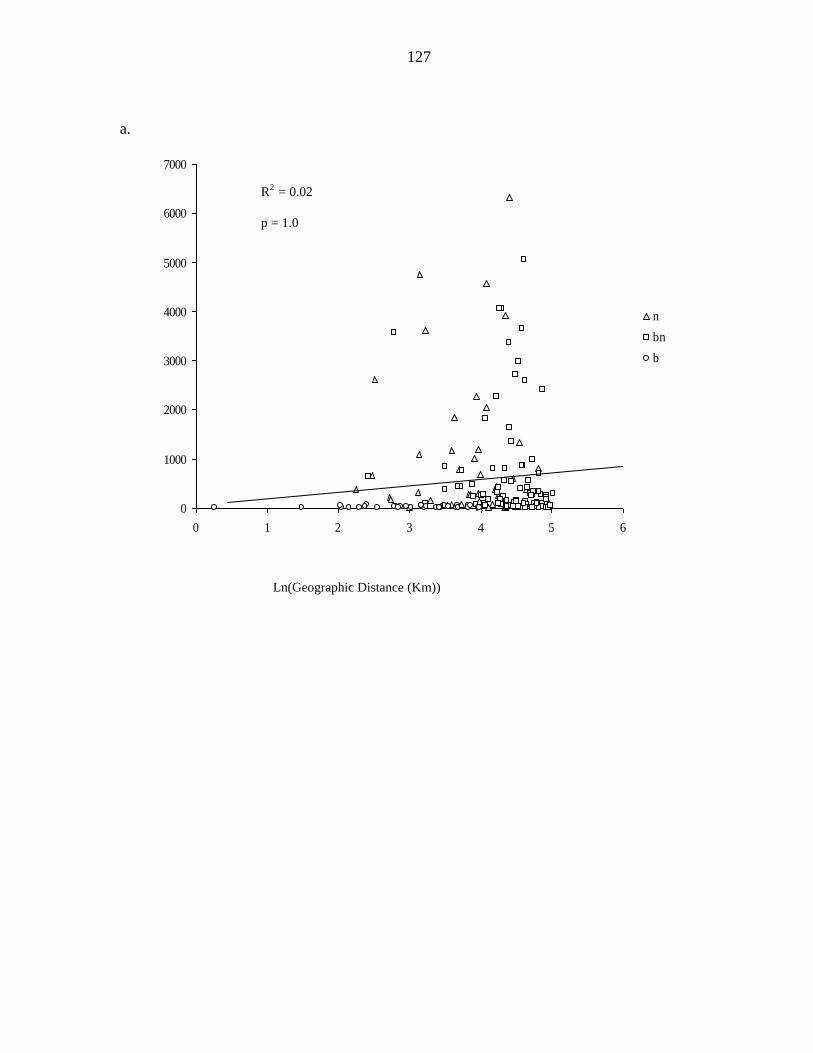
127

a.

0

1000

2000

3000

4000

5000

6000

7000

0 1 2 3 4 5 6

n

bn

b

Ln(Geographic Distance (Km))

R2

= 0.02

p = 1.0

128

b.

0

100

200

300

400

500

600

700

800

0 1 2 3 4 5 6

b

bn

n

R2 = 0.014

p = 0.99

Sq

uar

ed C

avit

y D

ista

nce

Ln(Geographic Distance (Km))

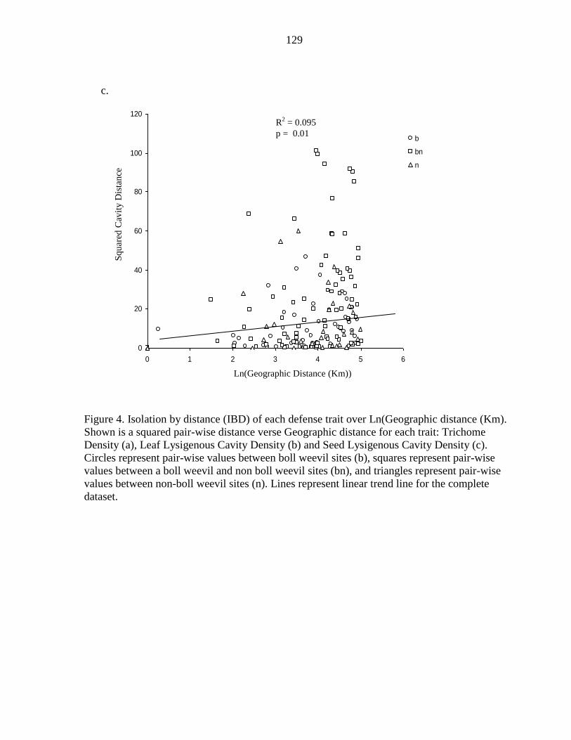
129

c.

Figure 4. Isolation by distance (IBD) of each defense trait over Ln(Geographic distance (Km).

Shown is a squared pair-wise distance verse Geographic distance for each trait: Trichome

Density (a), Leaf Lysigenous Cavity Density (b) and Seed Lysigenous Cavity Density (c).

Circles represent pair-wise values between boll weevil sites (b), squares represent pair-wise

values between a boll weevil and non boll weevil sites (bn), and triangles represent pair-wise

values between non-boll weevil sites (n). Lines represent linear trend line for the complete

dataset.

0

20

40

60

80

100

120

0 1 2 3 4 5 6

b

bn

n

Sq

uar

ed C

avit

y D

ista

nce

Ln(Geographic Distance (Km))

R2 = 0.095

p = 0.01

130

Table S1. Estimates of Weir and Cockeram’s (1984) FST for G. davidsonii using null allele-

adjusted (ENA) and unadjusted estimates. Adjustments for null alleles (ENA) were

calculated with FreeNa (Chapuis and Estoup, 2007).

GD Locus FST not using ENA FST using ENA

1 0.22614 0.196236

2 0.265597 0.257589

3 0.192863 0.176626

4 0.072824 0.071741

5 0.323829 0.308725

6 0.238808 0.219409

Overall 0.218713 0.202737

FST lower (95%) 0.158515 0.142022

FST upper (95%) 0.269448 0.253974

131

Table S2 . Information per locus within G. davidsonii of number of populations where

scoring errors due to Large Allele Dropout, Stutter Peaks, Null Alleles (as a result of excess

homozygosity) were detected in Microchecker (Oosterhout, 2004) and percentage of missing

genotypes for 21 populations.

Locus

Large Allele

Dropout

Stutter

Peaks

Null

Alleles

Missing Genotypes

(%)

GD1 0 4 17 3

GD2 0 4 14 6

GD3 0 5 12 5

GD4 0 1 4 13

GD5 0 5 10 2

GD6 0 2 8 2

132

Table. S3. Probability (P) values for Chi-Square test of Hardy Weinberg Equilibrium and FIS

estimates per population over all loci for G. davidsonii. Tests were performed by population

over all loci.

Population FIS P

19.1 0.503 ** 0.000 **

19.2 0.263 * 0.004

19.3 0.606 ** 0.000 **

19.4 0.218 ** 0.000 **

96 0.125 0.019

141 0.692 ** 0.000 **

142 0.622 ** 0.000 **

151 0.563 ** 0.000 **

160 0.197 0.000 **

162 0.516 ** 0.002 *

163 0.666 ** 0.000 **

164 0.623 ** 0.000 **

165 0.233 0.019

CP 0.354 * 0.000 **

LB 0.249 0.033

MG 0.127 * 0.000 **

RIB2 0.346 * 0.000 **

SB 0.789 ** 0.000 **

Shrine 0.49 * 0.000 **

TC 0.434 0.000 **

WC 0.441 ** 0.000 **

Mean 0.431286 **

*P = 0.05

**P = 0.01

133

Table S4. Analysis of Variance (ANOVA) tables for each defense trait. Shown are the effects

of Region, Population and within population error for each measured trait. Region was

defined as sites with or without boll weevil. Also shown are the sums of squares, F, and

probability of greater F for each effect.

Trait Source DF Sums of Squares F P >

Seed Lysigenous Cavity

Region 1 37.86 2.9144 0.088

Population 18 5117.58 21.888 <0.001

Error 532 6910.33 12.989

Total 551 12208.33 <0.001

Leaf Trichome

Region 1 464.79 7.230 0.008

Population 20 13083.69 10.176 <0.001

Error 305 19607.71 64.288

Total 326 33245.14 <0.001

Leaf Lysigenous Cavity

Region 1 109.04 0.428 0.514

Population 19 61802.30 12.766 <0.001

Error 222 254.80

Total 242 119726.85 <0.001

134

a.

b.

c.

0

0.1

0.2

0.3

0.4

0.5

0.6

0.7

0 0.2 0.4 0.6 0.8 1 1.2

h 2 between

Pse

udo

-QS

T

0.25

0.5

0.75

1

0

0.1

0.2

0.3

0.4

0.5

0.6

0.7

0.8

0.9

0 0.2 0.4 0.6 0.8 1 1.2

h 2 between

Pse

udo

-QS

T

0.25

0.5

0.75

1

135

Figure S1. PST estimates adjusted for inbreeding and heritability. Heritability values chosen

to assess the response of PST were recommended by Gay et al. (2009) for (a) leaf lysigenous

cavity density (b) trichome density (c) seed lysigenous cavity density. Shown are Pseudo-QST

estimates adjusted by 4 different degrees of within-population values of heritability (0.25, 0.5,

0.75, 1.0) and a range of between population values of heritability from 0 to 1 (x-axis). To

adjust PST for heritability measures, we multiplied h2

between to the Vbetween variance

components and h2

within to the Vwithin component in the PST calculation described in the Data

Analysis section. Grey lines represent a 95% confidence interval around FST over 6 SSR

markers. Broad sense heritability estimates in previous work for pigment glanded density in

leaves and seed of cotton cultivars has ranged from 92-98% (leaf: Singh and Weaver 1971;

seed: Lee et al. 1977).

0

0.1

0.2

0.3

0.4

0.5

0.6

0.7

0.8

0.9

1

0 0.2 0.4 0.6 0.8 1 1.2

h2

between

Psu

edo-Q

ST

0.25

0.5

0.75

1

136

Figure S2. Population graph of 21 G. davidsonii populations, designed in Genetics Studio

(Dyer et al., 2004). Shown in black are populations that are not hosted and in grey those hosts

of the boll weevil. Connections represent significant partial correlation between populations

and nodes represent populations (size of the sphere reflects the allelic diversity within a

population and genetic variation from variation in population sample sizes).

137

CHAPTER 5. Covariation in the geographic genetic structures of a wild cotton, Gossypium

davidsonii, and associated boll weevil, Anthonomus grandis

A paper to be submitted to Genetica

Adam P. Kuester, Kyung Seok Kim, Thomas W. Sappington, John D. Nason

Abstract

Gene flow and genetic structuring of host and parasite populations can influence the

outcome of reciprocal coevolution. Here, we combine traditional and recently developed

procedures to quantify and compare the congruence of geographical patterns of inter-population

gene flow in a plant-herbivore system involving wild cotton, Gossypium davidsonii (family

Malvaceae), and boll weevil, Anthonomus grandis (family Cuculionidae). Using Simple

Sequence Repeats (SSRs) we genotyped populations of both species from ten co-sampled sites in

the Cape Region of Baja California, Mexico. We find a two-fold difference between plant and

herbivore in the degree of population differentiation and that methods detecting gene flow

revealed significant incongruence in the geographical network of ancestral gene flow. This

incongruence suggests that gene flow in the two species has been influenced by different

geographical barriers to dispersal. Surprisingly, contemporary gene flow inferred from Bayesian

and likelihood methods were greater among host than herbivore populations. The conflict of

relatively high genetic differentiation and contemporary gene flow in G. davidsonii likely

represents limited statistical power to distinguish immigrants from locals than recent increases in

migration. Contrary, low genetic structuring and evidence of infrequent migration among A.

138

grandis populations may reflect local adaptation to G. davidsonii ecotypes and reduced survival

of immigrants in non-natal host sites.

Keywords: Anthonomus, boll weevil, cotton, gene flow, genetic structure, Gossypium

Introduction

Phytophagous insect species exhibit substantial variation in host breadth. Specialist

herbivores typically exhibit specificity to one or a few closely related host species and often

associated adaptations for feeding or reproduction on certain hosts (Nitao, 1989; Bernays, 1991;

Bowers et al., 1992; Oppenheim and Gould, 2002). In turn, patterns of dispersal and gene flow in

specialist insects are likeley to be strongly influenced by the need to locate the specific plant

species or ecotype to which it is adapted. Generalist herbivores, in contrast, have broader diets

than specialists, ranging from a few to several hundred hosts species, though generalists may also

exhibit a degree of specialization associated with geographical variation in available hosts (Potter

and Held, 2002).

It is unclear, however, whether specialists and generalists should be expected to exhibit

consistent differences in dispersal and genetic structure. On the one hand, suitable host plants for

specialists may be patchily distributed with individual insects typically having to disperse longer

distances to locate suitable host resources. On the other hand, if resources are patchy, specialists

within a host patch may exhibit only very localized movement, reflecting the need to minimize

fitness costs and risks associated with inter-patch dispersal. Conversely, suitable hosts for

generalists are likely to be less patchy, decreasing the intensity of selection for long-distance

139

dispersal. But because resources are more abundant, we might also expect lower fitness costs

associated with inter-patch dispersal and hence less selection against longer distance dispersal.

Although several studies have attempted to address the issue, the extent to which host-

specialization in plant feeding insects affects dispersal, gene flow and the evolution of population

genetic structure remains unclear (Peterson and Denno, 1998; Kelley, Farrell, and Mitton, 2000;

Smith et al., 2009). In contrast to insects, gene flow in plants is determined by the dispersal of

two different types of propagules: pollen and seed. Pollination syndrome and mating system have

been found to have a significant impact on the distribution of genetic variation within and among

plant populations (Hamrick and Godt, 1989). Stronger genetic structure (lower variation within

and greater differentiation among populations) is typical of species with animal as opposed to

wind pollination, and selfing as opposed to out-crossing mating systems. Although of weaker

effect, seed dispersal syndrome is also associated with differences in genetic structure. Species

dispersing seeds by gravity, for example, have greater genetic structure than species possessing

specialized adaptations for wind- or animal-mediated seed dispersal (Hamrick and Nason, 1996;

Dick et al., 2008). Thus, there is perhaps greater predictability in relating life-history

characteristics to genetic structure in plants than in their associated insect herbivores.

Recent studies suggest that patterns of gene flow within interacting species can be an

important determinant of their coevolutionary dynamics (Thompson and Burdon, 1992; Nuismer,

Thompson, and Gomulkiewicz, 1999; Forde, Thompson, and Bohannan, 2004; Hoeksema and

Forde, 2008; Vogwill, Fenton, and Brockhurst, 2008; Gandon and Nuismer, 2009). Indeed, that

out-comes of inter-species interactions are influenced by the level and spatial patterning of gene

flow between the populations of both species is a central component of the geographic mosaic

theory of coevolution (Thompson, Higgins, and Gibson, 1994; Thompson, 2005; Gomulkiewicz

140

et al., 2007). In plant-insect systems, the nature of the inter-specific interaction can influence the

amount and geographical symmetry of gene flow between populations of both organisms. In

particular, interactions in which an insect directly affects plant dispersal through pollination and

seed distribution are more likely to contribute to the geographical symmetry of gene flow

between the two species. Regardless of this symmetry, very low rates of gene flow within taxa

tend to limit local adaptive genetic variation and the rates of coevolutionary change, while very

high levels of gene flow can cause local maladaptation by limiting the effectiveness of reciprocal

selection. Theoretical studies indicate, however, that with greater symmetry of gene flow

between symbionts, localities with stronger reciprocal selection tend to dominate global

coevolutionary patterns (Nuismer, Thompson, and Gomulkiewicz, 1999; Gomulkiewicz et al.,

2000). For example, if gene flow is moderate (e.g., the probability of migration is m = 0.1) and

selection is stronger in coevolutionary “hot spots” (where fitness interactions are reciprocal) than

cold spots, then local dynamics in both hot and cold spots are expected to resemble the dynamics

of an isolated hot spot, and vice versa. In contrast, asymmetries in gene flow, as may be more

characteristic of antagonistic interactions involving plants and phytophagous insects, have been

shown to influence local adaptation by stabilizing coevolutionary equilibria at which a species

experiences minimal fitness in hot spots and maximal fitness in cold spots, or vice versa.

With increased interest in gene flow in coevolving taxa, network models of genetic

connectivity among populations are needed to address the symmetry of gene flow between

interacting species. Recent statistical genetic developments (Dyer and Nason, 2004; Dyer, 2007)

now enable us to reconstruct spatial networks of effective gene flow within species and to test for

the geographical symmetry of this gene flow between co-distributed taxa. In this paper, we

combine traditional, network-based, and Bayesian and likelihood methods to investigate the

141

magnitude and geographical structuring of historical and contemporary gene flow in a plant-

herbivore system involving the wild cotton Gossypium davidsonii (family Malvaceae) and its

specialist herbivore the boll weevil, Anthonomus grandis (family Cuculionidae).

Methods

Study System- Wild New World cotton species have been well studied for their variation

in traits desirable in domesticated cotton (G. hirsutum and G. barbadense), such as fiber

production (Mei et al. 2004; Park et al., 2005), chemical defenses (Stipanovic et al., 1986;

Stipanovic et al., 2003), and seed oil content (Gotmare et al., 2004). Other aspects of their natural

history, however, are not well understood. On the one hand, many of the New World species

have large, showy flowers, suggesting that they are attractive for pollinators, have out-crossing

mating systems, and experience appreciable gene flow. On the other hand, studies of wild

cottons have found low levels of genetic variability within populations, including G. davidsonii

(AFLPs: Alvarez and Wendel, 2006; allozymes: Wendel and Percival, 1990), suggesting that

cottons have intrinsically high levels of inbreeding via selfing and restricted gene flow. Studies

addressing this conflict have yet to be conducted for any wild cotton species. In Baja we have

observed G. davidsonii flowers to be visited by introduced European honey bees and by solitary

native bees and bombyliid flies (pers. obs.). Movement of seed within G. davidsonii is believed

to be mainly gravity and water dispersed (Stephens, 1958), but in Baja large introduced

ruminants feed on plants (pers. obs.) and may also disperse some seed.

The boll weevil, A. grandis, has been extensively studied on domesticated cotton, both in

the Southeastern United States and in Mexico, but is also found on many wild cotton host species,

including G. davidsonii (Cross, 1973). The boll weevil undergoes complete development within

142

the flower buds or fruits of cotton plants (Burke et al., 1986). Population genetic studies of A.

grandis populations on domesticated cotton cultivars have shown patterns of isolation by

distance and high levels of recent gene flow among boll weevil populations (Kim and

Sappington, 2004b; Kim and Sappington, 2006). In Baja California’s southern Cape Region, A.

grandis is a specialist on G. davidsonii, feeding on and developing within its fruits.

Site Sampling- Gossypium davidsonii and A. grandis populations were co-sampled at ten

sites in the Cape Region of the Baja Peninsula (Supplemental Table S1 and Figure 1). In the

southern portion of the Cape Region, where G. davidsonii is more densely distributed than in the

rest of its range, study sites were situated at least 8 km apart. Young, undamaged leaves were

collected from each sample plant, dried in silica gel, and stored at -80 °C until use for

microsatellite analysis. We sampled at least 13 plants per site (mean: 19, range: 13- 31, Table

S1).

Boll weevil larvae, pupae and adults were hand-collected from developing cotton bolls

(fruit) of G. davidsonii plants. We sampled weevils from at least 10 plants per site to promote

independence in sampling. Because females tend to oviposit multiple times on the same plant

and we often found multiple individuals per boll, for statistical independence we only sampled

one individual per fruit. All insects were stored in 95% ethanol and then at -80 °C until

processed for genetic analysis. Because we detected A. grandis only within a portion of G.

davidsonii’s range - the extreme south of the Cape Region - we focus here on these southern

locations where the two species co-occur. Collections of boll weevils ranged from 11 to 61

individuals per site (mean: 23, Table S1).

Gossypium davidsonii Microsatellite Genotyping- DNA was isolated from 15 mg of

silica-dried leaf material which was ground using a Genogrinder 2000 and extracted using aN

143

Autogen Autogenprep 740 DNA extraction robot (Holliston, MA) at the Iowa State University

DNA Facility. All DNA samples were eluted in water. DNA Concentration was determined by

spectrophotometry and dilutions of 20 ng/ul were prepared for use in Polymerase Chain

Reactions (PCR).

Of 50 Simple Sequence Repeat (SSR) loci screened from the Cotton Marker Database

(www.cottonmarker.org; Blenda et al., 2006) (Table S2), we identified 6 loci (GD1-GD6) as

polymorphic and suitable for multiplexing in G. davidsonii (Table 1). All of these markers were

derived from G. hirsutum and developed by Delta Pine Land (Wintersville, MS). Forward

primers were attached to an M13 tag for cost-effective fluorescent allele calling (Schuelke, 2000).

A mixture of labeled M13 tag primer and the sense primer were combined in a ratio of 15:1. All

primers were obtained from Integrated DNA Technologies (Corralville, IA).

Because fragment size overlap inhibited running all 6 SSR loci together in one reaction,

they were split into two multiplexes of 3 loci each. One multiplex consisted of 2μM GD1 and 3

μM each of GD2 and GD3. The other multiplex consisted of 2 μM GD5 and 3 μM each of GD6

and GD4. For each reaction, 40 ng of genomic DNA was used in 10 μl reactions with 0.2 μM

Promega dNTPs (Madison, WI), 2.5 μM MgCl2 (Bioline, Taunton, MA), 1X NaCl Buffer

(Bioline, Taunton, MA), and 0.4 units Bioline Taq DNA Polymerase (Taunton, MA). A MJ

Research Programmable Thermal Controller-100 (Waltham, MA) thermocycler was used for all

PCR reactions. Thermocycler conditions consisted of 95 ºC for 3min, 35 cycles of 94 ºC for 30 s,

50 ºC for 90 s, 72 ºC for 60 s, and a final extension at 72 ºC for 10 minutes. Samples that failed

to amplify were run a second time for verification. One μl of PCR product was used for fragment

detection using an Applied Biosystems 3730 DNA Analyzer (Carlsbad, CA) at the Iowa State

University DNA Facility. An ABI GS500 size standard was used for fragment length comparison.

144

All sample genotypes were analyzed using Applied Biosystems (Carlsbad, CA) PeakScanner 1.0

analytical software. A PP (Primer Peaks adjustment) sizing default was used for the analysis.

Anthonomus grandis Microsatellite Genotyping- Boll weevil DNA was extracted either

from whole body or head capsule using the Qiagen Tissue Prep kit, as described by Kim and

Sappington (2004a). DNA quality and quantity were determined by spectrophotometry and

dilutions of 20 ng/μl were prepared for use in PCR.

Individuals were genotyped at 10 SSR loci described in Kim and Sappington (2004a)

(Table 2). Primers for all loci were obtained from Proligo (Saint Louis, MO), with labeled Well-

Red dye on the forward primer for each locus. PCR reactions for all boll weevil amplifications

used Qiagen Master Mix and genotyping was conducted on a Beckman-Coulter (Brea, CA) CEQ

8000. All PCR reactions were performed using the touchdown thermocycling method described

in Kim and Sappington (2004a). All genotypes were analyzed with proprietary genetic analysis

system software v 8.0 developed for the CEQ 8000 Series, using default analysis parameters.

Microsatellite Data Analysis

Genetic Diversity and Differentiation- We used MicroChecker (Van Oosterhout et al.,

2004) to evaluate our scoring of G. davidsonii and A. grandis SSR genotypes for potential

scoring errors resulting from stuttering, large allele drop out, and null alleles (DeWoody,Nason,

and Hipkins, 2006). While A. grandis is dioecious and obligately outcrossing, members of genus

Gossypium are bisexual and are suspected of having high selfing rates and inbreeding. As a result,

excess homozygosity is expected for G. davidsonii populations at all loci and the presence of null

alleles cannot be inferred by the standard approach, employed by MicroChecker, of testing for

excess homozygosity that is evenly distributed across homozygote classes. Instead, we consider

as likely qualitative evidence of a locus having null alleles a level of deviation from HWE (or

145

inbreeding, FIS) that is exceptional relative to that of the majority of remaining loci. When we

were unable to amplify a locus within an individual after at least two attempts, we scored the

genotype at that locus as missing data and recorded the frequency of missing data for each locus

within G. davidsonii and A. grandis. Loci that amplified were independently scored twice to

check for scoring accuracy and we recorded the scoring error rate for each locus within both

species.

The number of alleles (Na), allelic richness, and observed and expected heterozygosity

(Ho and He, respectively) were assessed using FSTAT version 2.9.3 (Goudet, 2001) for both

species. Each SSR locus in each population of G. davidsonii and A. grandis was tested for

Hardy-Weinberg Equilibrium (HWE) using the Hardy Weinberg Exact Test in Genepop on the

Web (Sub-option 3: Probability test; Raymond and Rousset, 1995; Rousset, 2008). Microsatellite

loci were also tested for linkage disequilibrium for each pair of loci in each population using the

genotypic linkage disequilibrium test with default Markov chain parameters in Genepop. Since

multiple tests were performed in detecting deviation from both HWE and LD, a sequential

Bonferroni correction (Rice, 1989) was used to determine the significance of each test.

We used Wright’s F-statistics (Wright, 1965) to determine the degree of population

genetic structuring in both species. Using the methods of Weir and Cockerham (1984) we

estimated FIS as a measure of inbreeding within local populations and FST as a measure of genetic

differentiation among populations. These F-statistics were calculated for each locus and over all

loci using SPAGeDi-1.2 (Hardy and Vekemans, 2002) with 1000 permutations to detect

significant deviations from zero, and 1000 jackknife replicates to construct 95% confidence

intervals around estimates of FST. Although FST values are often compared between species, this

is problematic because FST is sensitive to differences between species in levels of genetic

146

variation at the marker loci used (Hedrick, 1999; Jost, 2008). Therefore, to use FST to test for a

difference between G. davidsonii and A. grandis in the level of population genetic differentiation,

we adjusted upper and lower 95% confidence limits on FST relative to maximum values of FST,

using the method of Hedrick (2005; equation 4b). We interpreted non-overlapping adjusted

confidence limits between species as indicative of a significant difference in population

differentiation.

We also obtained single and multilocus estimates of RST for both species and conducted

the permutation test of Hardy et al. (2003) to determine whether they are indicative of a stepwise

mutation process. These tests (conducted in SPAGeDi-1.2) were not significant and so we follow

the recommendation of Hardy et al. (2003) and report only estimates of FST since they have

lower variance than estimates of RST.

To account for any potential null allele effects on the estimation of FST, for both species

we used the program FreeNA (Chapuis and Estoup, 2007) to obtain estimates of FST adjusted for

null alleles (i.e., excluding null alleles) and not-adjusted for null alleles. Since both estimates of

FST were similar in both species (Tables S4 and S5, Supplemental Information), we report only

FST not adjusted for null alleles. We used a hierarchical AMOVA to estimate the level of genetic

differentiation within and among populations of A. grandis and of G. davidsonii east and west of

the Sierra La Laguna Mountains to assess this mountain range as a potential barrier to gene flow.

We estimated FRT for A. grandis and G. davidsonii, comparing regional and total variance, using

an AMOVA conducted using Arlequin v 3.1 (Excoffier et al., 2005).

Historical Gene Flow- For both G. davidsonii and A. grandis isolation by distance was

tested by regressing population pairwise estimates of linearized FST (FST/(1- FST) Rousset, 2000)

on the natural log of inter-population geographic distance using the Mantel test implemented in

147

the ISOLDE option of Genepop. We compared two geographic distance models, the Euclidean

distance between populations and a circum-montane distance that takes into account the Sierra

de la Laguna mountain range, which runs through the Cape Region, as a potential barrier to gene

flow in wild cotton and boll weevils (Jones et al., 1992). For populations separated by this

mountain range we calculated distances through a point (N 22.9795°, W 109.8846°) located at

the southern end of the range. The geographical distance model having the lower p-value and

higher coefficient of determination (R2) was selected as preferred. We also tested for isolation by

distance by regressing conditional genetic distance (cGD) on spatial distance under the two

geographic distance models. Dyer, Nason, and Garrick (2010) have shown that the use of cGD,

which is obtained from a Population Graph (Dyer and Nason, 2004), results in more powerful

tests of isolation by distance than those using linearized FST. Population Graphs were obtained

using GeneticStudio (Dyer, 2009). To gain further insight into overall rates of gene flow we

estimated the overall average number of migrants per generation among populations using the

private alleles method of Barton and Slatkin (1986).

In addition to the more traditional methods described above, we used Population Graphs

(Dyer and Nason, 2004; Dyer, 2007), a network-based method, to quantify spatial patterns of

effective gene flow among populations. A Population Graph consists of nodes (populations), a

subset of which are connected by edges representing significant conditional genetic covariation

between the linked population pairs. The Population Graphs used in these analyses were obtained

using GeneticStudio and provide a spatially explicit model of ancestral gene flow connecting

populations of each species.

Contemporary Gene Flow- We quantified immigration and emigration for both species

using two complementary methods, GeneClass2 (Piry et al., 2004) and STRUCTURE v. 2.2.3

148

(Pritchard, Stephens, and Donnelly, 2000). Both methods assign migrants to specific sample

populations, but because it was not possible to sample all potential source populations, we

interpret these results as indicative of migration events and immigration rates, but not of the

population origin of migrants. Our primary objective in using these two methods was to

determine whether the boll weevil has rates and patterns of migration that are similar to that of

its host plant, G. davidsonii. We evaluated the results of the two methods for their agreement in

identifying immigrant individuals.

In GeneClass2 we used the test statistic Lh, which is the likelihood of drawing an

individual’s genotype from the population in which it was sampled, given the observed set of

allele frequencies. Following a statistical approach of Rannala and Mountain (1997) and a

resampling approach described by Paetkau et al. (2004), we used used “Detection as First

Generation Migrant” Criteria, using the test statistic Lh- Paetkau et al. (2004) recommend use of

Lh when not all potential source populations have been sampled, which is the case in our study.

In the case where a sampled migrant did not originate from any of the sampled populations, it

will tend to be recognized as a resident, since Lh and the most likely source population (Lmax) will

have similar likelihood values. For A. grandis we detected no migrants using Lh and so repeated

the analysis using Lh/ Lmax, which has greater power to detect migrants (Paetkau et al., 2004).

Critical values for rejecting the null hypothesis that an individual was born in the population

from which it was sampled were generated using Monte Carlo resampling in GeneClass2. We

used an alpha level of 0.01 in determining critical values, as recommended by Paetkau et al.

(2004).

In using STRUCTURE v. 2.2.3 we were specifically interested in identifying immigrants

into sample populations and so defined the number of inferred clusters or groups (K) as equal to

149

the number of sampled populations, K=10. We also employed the admixture model, which

allows individuals to inherit their genome from one or more of the K groups, and the

USEPOPINFO option, which assumes a relatively high prior probability that an individual

originates from the population in which it is resident. This strategy results in analyses that are

conservative with respect to the inference of migration events. We performed 20 individual runs

of STRUCTURE to determine convergence, with a burn-in of 10,000 and 100,000 iterations. The

estimated membership coefficient for each individual in each of the K inferred groups, Q, was

estimated by STRUCTURE. Vähä and Primmer (2006) used a threshold Q of 0.8 to classify

individuals as local, with lower Q values used to classify individuals as mixed via gene flow. In

our study, for G. davidsonii we classified individuals as local for Q ≥ 0.8, and as immigrants

otherwise. For A. grandis we detected very few (typically 0) immigrants per populations and so

increased the threshold for classfying individuals as local to Q ≥ 0.9, making the analysis slightly

less conservative regarding the identification of immigrants.

Since the detection of migration using STRUCTURE can be sensitive to the migration rate

prior (MIGRPRIOR) when the actual migration rate is low (Pritchard and Wen, 2004), we ran

STRUCTURE using MIGRPRIOR in the range m = 0.001 to 0.1, as suggested by Pritchard,

Stephens, and Donnelly (2000). For G. davidsonii we found differences between runs using the

extreme values of MIGRPRIOR, so we present results for both m = 0.001 and 0.1. For A. grandis

we did not see differences in group assignment for values spanning the range m = 0.001 to 0.1,

so present results for the prior value m = 0.05.

Hardy-Weinberg equilibrium is used as an optimality criterion in STRUCTURE and natural

inbreeding can cause it to over-estimate the number of groups and to falsely assign individuals to

multiple groups (Gao, Williamson, and Bustamante, 2007). Since G. davidsonii is believed to

150

have substantial inbreeding (confirmed here) we also assessed population structure using

InStruct (Gao, Williamson, and Bustamante, 2007), which relaxes the Hardy-Weinberg

assumption of no inbreeding when clustering individuals to groups. We used similar parameters

as for the STRUCTURE analysis (without incorporating USEPOPINFO), but allowed InStruct to

estimate the population-level inbreeding coefficient and evaluate 2 runs of 5 chains each.

Because InStruct identified most individuals of both species as immigrants, a biologically

unlikely scenario, we present only the more conservative estimates provided by STRUCTURE

utilizing the USEPOPINFO option.

Comparative Analyses of Gene Flow- Within G. davidsonii and A. grandis we compare

patterns of migration inferred by GeneClass2 and STRUCTURE by means of a Mantel test of

adjacency matrices in which element ij is equal to 1 if there is one or more inferred migration

event from sample population i to j, and 0 otherwise. We similarly conducted a Mantel test of

migration rate matrices in which element ij equals the number of inferred migrants from sample

population i to j. For both tests a positive Mantel correlation is expected if GeneClass2 and

STRUCTURE indicate similar patterns of migration. We also compared the pattern of historical

gene flow reflected in the topology of a Population Graph to the pattern of contemporary gene

flow inferred by GeneClass2 and STRUCTURE. We did this by conducting two Mantel tests: one

of adjacency matrices comparing connections between populations, and one of the cGD matrix

obtained from the Population Graph versus the migration rate matrix obtained from GeneClass2

or STRUCTURE. In the latter test, we expect a negative correlation if the two methods indicate

similar patterns of gene flow.

To determine whether the spatial patterning of inter-population gene flow is correlated

between co-sampled G. davidsonii and A. grandis populations we performed Mantel tests on

151

adjacency matrices and on migration rate matrices obtained from GeneClass2 and STRUCTURE.

We also conducted Mantel tests of adjacency and cGD matrices obtained from Population

Graphs. In all of these tests we expect a positive correlation when inferred patterns of genetic

connectivity are similar between species.

To further assess the congruence of population genetic structure between species,

neighbor-joining trees for G. davidsonii and A. grandis were constructed using Cavalli-Sforza’s

chord distance in Phylip v 3.69 (Felsentstein, 2004), with 1000 bootstrap randomizations used to

determine branch support. Topological congruency between trees was assessed using Icong

(index of congruency) (Vienne, Giraud, and Martin, 2007), which tests the null hypothesis that

the topologies of two compared trees are not more identical than expected by chance. This

method determines the number of changes required to make one tree’s topology identical to the

other, using trees of randomized leaf organization to construct the null distribution of this

statistic

Results

Genetic Diversity and Differentiation- Independently scoring each G. davidsonii

genotype twice resulted in a scoring error rate of 2.6%. Scoring errors from stutter peaks and

large allele drop-out were not detected by MicroChecker for any G. davidsonii population or

locus. The per locus frequency of missing genotypes after re-amplification ranged from 0.021 to

0.120 with a mean of 0.049 across loci (Table S3). These percentages may indicative of low

frequencies of null alleles. Given the presumed mixed-mating system of G. davidsonii, it is not

surprising that MicroChecker identified all six loci as exhibiting excess homozygosity and,

therefore null alleles, within at least one population (Table S3). In multilocus tests using

152

Genepop, after sequential Bonferroni correction we found significant deviations from HWE in

eight of ten G. davidsonii populations (all tests with P < 0.005), the exceptions being sites 165 (P

= 0.014) and 19.4 (P = 0.005), which also exhibited excess homozygosity (Table S4,

Supplemental Information). FIS values averaged across loci for individual populations ranged

from 0.237 to 0.630 (Table S4). Similarly, FIS values averaged across populations for individual

loci ranged from 0.392 to 0.647 (Table 1). An exception was locus GD4 for which FIS was 0.013.

Given the relatively low FIS estimate for GD4 we repeated all of analyses excluding this locus

and, for comparison of effects, excluding each other locus in turn. We observed small losses of

statistical power (increases in variance) consistent with the reduction in loci but otherwise did

not find the conclusions obtained excluding GD4 to differ from those obtained excluding any

other locus. Furthermore, we found the FST = 0.069 for GD4 to be within the range for the

remaining loci (0.063-0.154; Table 1), which is important given that this study focusses

primarily on inter-population differentiation. As a result of these observations, all results we

report for G. davidsonii include the use of GD4.

Allelic diversity in G. davidsonii ranged from 4-7 alleles per locus, allelic richness

ranged from 2.512- 3.647 (mean AR = 3.067), and gene diversity ranged from 0.310-0.633 (mean

He = 0.477, Table 1). We observed relatively similar levels of genetic differentiation among

populations for the different loci (mean FST = 0.120, P < 0.001, Table 1). In global tests across

populations one of 15 locus pairs (GD5 and GD6) exhibited significant evidence of linkage

disequilibrium after sequential Bonferroni correction (χ2=41.1, P = 0.001).

For boll weevil, across loci we found an error rate of 3.4% in re-scoring multilocus

genotypes. Large allele dropout was not observed in any population by locus combination but

MicroChecker did detect potential scoring errors due to stutter peaks in 0 to 3 populations per

153

locus (Table S3). MicroChecker indicated excess homozygosity that was evenly distributed

across homozygote classes, indicative of the presence of null alleles, in 0 to 3 populations per

locus (Table S3). Consistent with a low frequency of null alleles, the per locus frequency of

missing data after re-amplification ranged from 0.068 to 0.153 with an average of 0.119 across

loci (Table S3).

In testing for HWE in A. grandis, we found that all populations but three (142: P = 0.034,

MG: P = 0.264; WC, P = 0.280) exhibited significant multilocus deviations after sequential

Bonferroni correction (Table S4), and population-level estimates of FIS ranged from 0.026 to

0.424 (Table S4). Locus-specific estimates of FIS ranged from -0.102 to 0.409 for 8 of the ten

loci (Table 2). For the remaining two loci, BW21 and BW35, FIS estimates were higher (0.725

and 0.635, respectively), leading us to repeat our analyses excluding these two loci. Because

these two loci had very low genetic diversity (He = 0.060-0.070; Table 2) losses of statistical

power were negligible. Furthermore, the high FIS estimates for these two loci were entirely

attributable to a small number of rare homozygotes (BW21: 4 rare homozygotes in 3 populations;

BW35: 3 rare homozygotes in 3 populations). As a result of these observations, all results we

report for A. grandis include the use of BW21 and BW35.

Data sets that were corrected and uncorrected for null alleles (using FreeNA) yielded

nearly identical multilocus average FST estimates and confidence intervals in G. davidsonii

(Table S5) and in A. grandis (Table S6).

Levels of genetic variation in A. grandis were similar to those observed in G. davidsonii,

with the number of alleles per locus ranging from 2 to 8, allelic richness from 1.225 to 2.982

(mean 2.186), and gene diversity from 0.060-0.594 (mean He = 0.416, Table 2). FST for A.

grandis was significantly greater than zero (mean FST = 0.058, p < 0.001) and, using Hedrick

154

(2005) adjusted values, significantly less than estimated for G. davidsonii (adjusted FST and 95%

confidence intervals - A. grandis: 0.127 (0.096 - 0.157); G. davidsonii: 0.339 (0.209 - 0.469)). In

global tests across populations, one of 45 locus pairs (BW43 and BW9) exhibited significant

linkage disequilibrium after sequential Bonferroni correction (χ2

= 103.66, P < 0.001).

Gene Flow- We found no evidence of isolation by distance among G. davidsonii

populations using either Euclidean (linearized FST: R2 = 0.008, P = 0.237; cGD: R

2 = 0.007; P =

0.265) or circum-montane (linearized FST: R2 = 0.009, P = 0.24; cGD: R

2 = 0.008; P = 0.440)

distance models. Similarly, isolation by distance among boll weevil populations was not

significant using either Euclidean (linearized FST: R2= 0.049, P = 0.127; cGD: R

2 = 0.007; P =

0.715) or circum-montane (linearized FST: R2

= 0.050, P = 0.127; cGD: R2 = 0.008; P = 0.234)

distance. We found low, but significant, regional genetic differentiation between the east and

west sides of the Sierra La Laguna for G. davidsonii (FRT= 0.017, P = 0.005), but not for A.

grandis (FRT= -0.014, P = 0.987).

Population graphs for G. davidsonii and A. grandis both contained 14 significant edges

(Figure 1c). Mantel correlations between G. davidsonii and A. grandis graphs were not

significant (adjacency matrices: r = 0.067, P = 0.375; cGD matrices: r = 0.094, P = 0.311).

Although inter-population genetic differentiation was lower in boll weevil, the private alleles

method indicated a lower migration rate of 1.6 individuals per generation in A. grandis as

compared to 3.56 individuals per generation in G. davidsonii.

Assignment testing with GeneClass2 inferred 14 migrants in G. davidsonii (Table 3),

There was no apparent pattern to the directionality of these inferred migration events, which

included movement across the Sierra La Laguna (Figure 1b). For A. grandis, GeneClass2

inferred 6 migration events (Table 3), 5 of which occurred along the west coast of the Cape

155

Region (Figure 1b). We found no significant correlation between species in inferred migration

events using either adjacency (r = 0.065, P = 0.776) or migration rate matrices (r = 0.08, P =

0.786).

A STRUCTURE analysis of G. davidsonii indicated 10 apparent migrant events. Of the 10

populations, 3 migrants were detected in WC, 2 from MG, and 1 each in populations 142, 164,

19.1, 19.2, and 19.3. STRUCTURE identified 9 migrants in A. grandis, 4 in population 19.2, 2 in

population 19.3 and one each in populations 164, MG, and 142. We found no correlation in the

geographical patterning of STRUCTURE inferred migration events in Mantel tests of connectivity

or migration rate matrices (connectivity: r = -0.153, P = 1.00; migration rate: r = -0.227, P =

1.00).

Comparing GeneClass2 and STRUCTURE results within species, the correlation across

study sites in inferred migration events was positively correlated in G. davidsonii (adjacency

matrix: r = 0.611, P = 0.003; migration rate matrix: r = 0.338, P = 0.003), but not in A. grandis

(adjacency matrix: r = -0.136, P = 1.000; migration rate matrix: r = -0.016, P = 1.000). Similarly,

GeneClass2 and STRUCTURE results were significantly correlated with Population Graph results

in G. davidsonii (GeneClass2 vs. Population Graph comparisons: migration rate vs. cGD: r = -

0.00356, P = 0.005; adjacency vs. adjacency: r = 0.592, P = 0.007; STRUCTURE vs. Population

Graph comparisons: migration rate vs. cGD: r = -0.00175, P = 0.034; adjacency vs. adjacency: r

= 0.295, P = 0.079), but not in A. grandis (GeneClass2 vs. Population Graph comparisons:

migration rate vs. cGD: r = 0.0001, P = 0.895; adjacency vs. adjacency: r = 0.221, P = 0.117;

STRUCTURE vs. Population Graph comparisons: migration rate vs. cGD: r = 0.0003, P = 0.399;

adjacency vs. adjacency: r = -0.318, P = 1.000).

156

Branch support within G. davidsonii and A. grandis neighbor-joining trees was generally

weak (Figure 2) and the topological congruence of the two trees was not significant (Icong =

7.45, P = 0.875).

Discussion

Genetic differentiation was significantly higher among G. davidsonii populations than among

A. grandis populations. This was an expected result given lower dispersal capabilities of the

plant (inbreeding and gravity dispersed seeds) in comparison to a flying insect. Interestingly,

given the small geographic range examined (slightly over 100 km) we were surprised to see

relatively high levels of genetic differentiation, especially in A. grandis. Boll weevil populations

from Texas have lower or insignificant amounts of genetic differentiation at much larger

geographic scales than observed here (Kim and Sappington, 2006). Additionally, Kim and

Sappington (2006) identified at least 3 boll weevil migrants exchanged between populations on

cultivated cotton located up to 300 km apart, whereas using similar estimations of effective

migrants (Nm), we calculate nearly 1.88 migrants per generation. In boll weevil associated with

domesticated cotton, migrants are known to be carried by wind currents with the potential for

long distance dispersal (Culin et al., 1990; Kim et al., 2010; Westbrook, Eyster, and Allen, 2011)

and patterns of movement may be affected by winds in the cape region. The direction of

migration observed in GeneClass2 for boll weevils on G. davidsonii occurred in a southerly or

southeasterly direction; we identified 4 of 6 inferred migration events consistent with prevailing

wind patterns from the north and west in Baja California Sur (Jaramillo, Saldana, and Miranda,

2004).

157

High levels of genetic differentiation within both A. grandis and G. davidsonii may suggest

that both species are locally adapted to population-specific environments. A. grandis populations

may be adapted to local host population phenotype characteristics. Both phenological and plant

defense phenotypes have been shown to affect insect herbivores hosted on cotton, such as

flowering time and boll development (Greenberg et al., 2004; Showler, 2005; Showler, 2008),

boll nutrient content (Hardee, Mitchell, and Huddleston, 1966), foliar trichome density (Percy

and Kohel, 1999), extrafloral nectary density (Rudgers et al., 2004) and gossypol content

(Jenkins, Maxwell, and Parrott, 1967; Bell et al., 1987; Hedin and McCarty, 1995).

If boll weevils disperse G. davidsonii pollen then there are potential benefits to cotton plants

of hosting boll weevils and, potentially, selection favoring phenotypes or genotypes attractive to

boll weevils and susceptible to attack. Though female boll weevils oviposit on developing fruit

and larvae feed on cotton seeds, larvae do not consume all seeds within individual G. davidsonii

capsules (pers. obs.). Rather, larvae typically form a small pupal capsule within one locule of the

cotton fruit. Karban and Lowenberg (1992) have shown experimentally that boll weevil and

other seed-feeding insect herbivores can promote germination of undamaged seed by scarifying

the seed coat prior to germination. Seed scarification is important in many xerophytic species

(Vilela and Ravetta, 2001). In fact, seeds that were not destroyed by seed-feeding insects had a

higher likelihood of germinating during the first wet season than unattacked seeds. This may be

one reason why Gossypium davidsonii is a dominant plant species in lower portions of the

peninsula rather than in more northern sites, where boll weevils are not present on G. davidsonii.

In general, the migration patterns of A. grandis individuals we observed were between

populations with similar plant defense phenotypes or trending to populations with higher mean

glands or decreased trichome densities (data unpublished). Previous work has shown that boll

158

weevils are attracted to gossypol (Hedin and McCarty, 1995) and that G. hirsutum accessions

with high levels of trichomes have been more effective at evading boll weevil infestations

(Matthews, 1989). Since we observed more boll weevil immigrants on higher or similar gossypol

levels using the GeneClass2 results, we might expect to find that defense traits in boll weevil

infested areas to be under stabilizing selection, to produce sufficient phenotypes to attract

weevils.

It was surprising to detect higher levels of contemporary migration within G. davidsonii,

given the fact that our estimate of genetic differentiation within the sampled range of the species

was significantly greater than for A. grandis. There are a few reasons that could explain high

differentiation, yet relatively high detection of migrants within G. davidsonii. We may be

observing an increase in migration, via seed and or pollen dispersal as a result of environmental

change. Though unlikely that recent human disturbance in the region has greatly influenced seed

dispersal, it is possible that increased development in the southern tip of the Baja Peninsula over

the past decades has affected frequency of pollinator visits. As seed dispersal mechanisms are

not expected to have been influenced by human activity, especially by increasing contemporary

inter-population migration, we believe changes in pollinator behavior is a more realistic

explanation of gene flow in the system. We have also found very high and significant genetic

differentiation between patches within sampled study sites, at the scales of under 2 km (FST =

0.171, P = 0.001) and as small as 100 m (FST = 0.202, P = 0.001) (data unpublished). Pollination

events from relatively close neighboring plants may appear to quite foreign, which might explain

relatively high levels of migrants detection within populations of the cotton. We might be

detecting dispersal between highly differentiated populations from relatively short distances

away of only a few hundred meters. Since our means of assignment merely detected non-local

159

genotypes, not their site of origin, we may have detected short-distance dispersal between highly

differentiated populations from relatively short distances away of only a few hundred meters.

Alternatively, detection of non-local individuals within populations could result from limitations

of population sample sizes.

Despite significant genetic differentiation among populations, we did not detect IBD in either

species, indicating that spatial patterns of gene flow both species may be relatively idiosyncratic

and inconsistent with steppingstone models of migration. Also somewhat surprising, assignment

tests inferred migrants among populations in both species, indicating levels of gene flow

potentially in conflict with observed levels of inter-population genetic differentiation. Given that

population sample sizes ranged from 13 – 31 (Table S1), the frequency of inferred migration

events suggests that the number of effective migrants per generation may be greater than the 2-3

expected for an observed FST = 0.12 under an island model of migration. As noted previously,

however, it is important to realize that the migrants identified by GeneClass2 and STRUCTURE are

not necessarily moving between study populations. Rather, they are individuals whose genotypes

have a relatively low probability of having arisen in the population in which they were sampled.

These individuals may thus represent migration events originating more locally than from other,

more distant study populations.

GeneClass2 and STRUCTURE analyses led to similar conclusions as to the number of migrants

among G. davidsonii populations. The two methods also consistently assigned the same

individuals as migrants per population. Though we did not see consistent results between the 2

methods from the A. grandis analyses, too few migrants were identified by either method to

confidently compare movement patterns.

160

We detected an incongruence of migrants between host and insect when comparing results

from both GeneClass2 and STRUCTURE, reflecting incongruent contemporary gene flow between

the two species. Lower levels of detected migration among boll weevil populations could have

been an artifact of sampling too few individuals per population, whereby larger population

sample sizes would have provided more accurate migrant determination. The accuracy

procedures used to detect contemporary gene flow are affected by sample size (Pritchard,

Stephens, and Donnelly, 2000; Piry et al., 2004). Alternatively, lower movement rates among

boll weevil populations may reflect association of boll weevils with native host populations. In a

situation that may be analogous, females persist on patchy volunteer cotton to oviposit on the

same host (Summy, Cate, and Bar, 1993). This pattern of interaction within small populations of

plant host may reflect an adaptation to avoid the risk of not finding suitable hosts elsewhere.

In comparing ancestral gene flow between the boll weevil and G. davidsonii sampled

populations, we, likewise, note incongruency of gene flow. Gene flow affects the extent to

which subpopulations evolve together as an evolutionary unit (Slatkin, 1994). Thus, high gene

flow among populations in divergent environments may prevent development of optimal

phenotypes or adaptations in either one. In both the cotton and boll weevil populations, 14

significant connections (presence of gene flow) were detected between pairs of populations. The

presence of genetic structuring among boll weevil populations associated with G. davidsonii, yet

incongruent patterns of gene flow compared to that of its host, is consistent with population-

specific host-association.

We detected similar patterns of connectivity in both ancestral and current gene flow in G.

davidsonii, suggesting the species has been evolving under similar rates of recurrent gene flow

over an extended period of time. On the other hand, we found no similarity between historical

161

and current gene flow patterns within A. grandis, which may be a reflection of historical host

availability. G. davidsonii has been documented as a dominant plant species in the southern Cape

region of the Baja Peninsula over the past 50 years (Phillips and Clements, 1967). However, it is

a dominant species in disturbed habitat (pers. obs.), so it is possible that its population sizes in

the sampled region have grown as a result of increased commercial development and, subsequent

greater habitat disturbances within the region, as the species is a dominant species in disturbed

habitat (pers. obs.). Increased population sizes within G. davidsonii, may have contributed to

greater current population structure among A. grandis populations, by providing more resources

within populations, reducing the need for A. grandis to find additional suitable hosts.

In summary, we observed significant genetic structuring within both host and associated

insect. High genetic structuring within G. davidsonii is believed to be in response to limited

dispersal capabilities of water dispersed seed and infrequent cross-pollination. On the other hand,

observed differentiation in the boll weevil might be interpreted as adaptation to host-specific

populations of cotton. We also found incongruence of both contemporary and ancestral gene

flow between the two species. Ecological studies examining reasons why observed migration

patterns will be necessary to determine whether movement reflects local adaptations of the boll

weevil to associated cotton host populations. Additional population genetic study of boll weevil

on wild cotton species will also elucidate whether observed migration patterns on G. davidsonii

are consistent across wild host species.

Literature Cited

Alvarez, I., and J.F. Wendel, 2006. Cryptic Interspecific Introgression and Genetic

Differentiation Within Gossypium aridum (Malvaceae) and Its Relatives. Evolution 60, 505-517.

162

Barton N.H., and M. Slatkin, 1986. A quasi-equilibrium theory of the distribution of rare alleles

in a subdivided population. Heredity 56, 409-416.

Bell, A., R. Stipanovic, G. Elzen, and H. Williams, 1987. Structural and genetic variation of

natural pesticides in pigment glands of cotton (Gossypium). In: Allelochemicals: Role in

Agriculture, Forestry and Ecology (ed. G Waller), p. 330. American Chemical Society

Symposium.

Bernays, E.A., 1991. Evolution of insect morphology in relation to plants. Philosophica

Transactions of the Royal Society of London B Biological Sciences 333, 257-264.

Blenda, A., J. Scheffler, B. Scheffler, M. Palmer, J.-M. Lacape , J.Z. Yu , C. Jesudurai ,S. Jung ,

S. Muthukumar, P. Yellambalase, S. Ficklin , M. Staton, R. Eshelman, M. Ulloa, S. Saha, B.

Burr, S. Liu, T. Zhang, D. Fang, A. Pepper, S. Kumpatla, J. Jacobs, J. Tomkins, R. Cantrell, and

D. Main, 2006. CMD: A Cotton Microsatellite Database Resource for Gossypium Genomics.

BMC Genomics 7, 132.

Bowers, M., M. Deane, N. Stampe, and S. Collinge, 1992. Early Stage of Host Range Expansion

By a Specialist Herbivores, Euphydryas phaeton (Nymphalidae). Ecology 73, 526-536.

Burke, H.R., W.E. Clark, J.R. Cate, and P.A. Fryxell, 1986. Origin and Dispersal of the Boll

Weevil. Bulletin Entomological Society America 32, 228-238.

Chapuis, M.P. and A. Estoup, 2007. Microsatellite null alleles and estimation of population

differentiation Molecular Biology and Evolution 24, 621-631.

Cornuet, J. and G. Luikart, 1996. Description and power analysis of two tests for detecting recent

population bottlenecks from allele frequency data. Genetics 144, 2001-2014.

Cross, W.H., 1973. Biology, Control, and Eradication of the Boll Weevil. Annual Review of

Entomology 18, 17-46.

Culin, J., S. Brown, J. Rogers, D. Scarborough, A. Swift, B. Cotterill, J. Kovach, 1990. A

simulation model examining boll weevil dispersal: historical and current situations. Environ

Entomol 19, 195–208.

DeWoody J., J.D. Nason, and V.D. Hipkins, 2006. Mitigating scoring errors in microsatellite

data from wild populations. Molecular Ecology Notes 6, 951-957.

Dick, C.W., O.J. Hardy, F.A. Jones, and R.J. Petit, 2008. Spatial Scales of Pollen and Seed-

Mediated Gene Flow in Tropical Rain Forest Trees. Tropical Plant Biology 1, 20-33.

Dyer, R.J. and J.D. Nason, 2004. Populations Graphs: The graph-theoretic shape of genetic

structure. Molecular Ecology 13, 1713-1728.

Dyer, R.J. 2007. The evolution of genetic topologies. Theoretical Population Biology 71, 71-79.

163

Dyer, R.J., 2009. GeneticStudio: A suite of programs for the spatial analysis of genetic marker

data Molecular Ecology Resources 9, 110-113.

Dyer, R.J., J.D. Nason, and R.C. Garrick, 2010. Landscape modeling of gene flow: Improved

power using conditional genetic distance derived from the topology of population networks.

Molecular Ecology 19, 3746-3759.

Felsenstein, J., 2004. PHYLIP (Phylogeny Inference Package) version 3.6. . Department of

Genome Sciences, University of Washington, Seattle.

Forde, S.E., J.N. Thompson, and B.J.M. Bohannan, 2004. Adaptation varies through space and

time in a coevolving host-parasitoid interaction. Nature 431, 841-844.

Gandon, S. and S.L. Nuismer, 2009. Interactions between Genetic Drift, Gene Flow, and

Selection Mosaics Drive Parasite Local Adaptation. The American Naturalist 173, 212-224.

Gao, H., S. Williamson, and C.D. Bustamante, 2007. An MCMC Approach for Joint Inference of

Population Structure and Inbreeding Rates from Multi-Locus Genotype Data. Genetics

176:1635-1651.

Garson, G., 1982. Political Science Methods. Holbrook, Boston, MA.

Gomulkiewicz, R., J.N. Thompson, R.D. Holt, S.L. Nuismer, and M.E. Hochberg, 2000. Hot

spots, cold spots, and the geographic mosaic theory of coevolution. The American Naturalist

156, 156-174.

Gomulkiewicz, R.D., D.M. Drown, M.F. Dybdahl, W. Godsoe ,S.L. Nuismer, K.M. Pepin, B.J.

Ridenhour, C.I. Smith, and J.B. Yoder, 2007. Dos and don’ts of testing the geographic mosaic

theory of coevolution. Heredity 98, 249-258.

Gotmare, V., P. Singh, C.D. Mayee, V. Deshpande, and C. Bhagat, 2004. Genetic variability for

seed oil content and seed index in some wild species and perennial races of cotton. Plant

Breeding 123, 207-208.

Goudet, J. 2001. FSTAT, a program to estimate and test gene diversities and fixation indices

(version 2.9.3).

Greenberg, S.M., T.W. Sappington, M. Setamou, and R. Coleman, 2004. Influence of Different

Cotton Fruit Sizes on Boll Weevil (Coleoptera: Curculionidae) Oviposition and Survival to

Adulthood. Environ. Entomol. 33, 443-449.

Greenberg, S.M., G.D. Jones, F. Eischen, R.J. Coleman, J.J. Adamczyk Jr, T. Liu, and M.

Setamou, 2007. Survival of boll weevil (Coleoptera: Curculionidae) adults after feeding on

pollens from various sources. Insect Science 14, 503-510.

164

Hamrick, J.L., and M.J. Godt, 1989. Allozyme diversity in plant species. pp 43-63 In Brown, A.

H. D., M. T. Clegg, A. L. Kahler and B. S. Weir (eds), Plant Population Genetics, Breeding and

Germplasm Resources. Sinauer, Sunderland, Mass.

Hamrick, J.L., and J.D. Nason, 1996. Consequences of dispersal in plants. Pp. 203-236 in OEJ

Rhodes, RK Chesser and MH Smith (eds.), Population Dynamics in Ecological Space and Time.

The University of Chicago Press, Chicago, Illinois, USA.

Hardee, D., E. Mitchell, and P. Huddleston, 1966. Effect of Age, Nutrition, Sex, and Time of

Day on Response of Boll Weevils to an Attractant from Cotton. Annals of the Entomological

Society of America 59, 1024-1025.

Hardy, O.J., and X. Vekemans, 2002. SPAGeDi: a versatile computer program to analyse spatial

genetic structure at the individual or population levels. Molecular Ecology Notes 2, 618-620.

Hardy, O.J., N. Charbonnel, H. Freville, and M. Heuertz, 2003. Microsatellite Allele Sizes: A

Simple Test to Assess Their Significance on Genetic Differentiation. Genetics 163, 1467-1482.

Hedin, P., and J. McCarty. 1995. Boll Weevil Anthonomus grandis Boh. Oviposition Is

Decreased in Cotton Gossypium hirsutum L. Lines Lower in Anther Monosaccharides and

Gossypol. Journal of Agricultural and Food Chemistry 43, 2735-2739.

Hedrick, P., 1999. Perspective: highly variable loci and their interpretation in evolution and

conservation. Evolution 53, 313-318.

Hedrick, P., 2005. A standardized genetic differentiation measure. Evolution 59, 1633-1638.

Hoeksema, J.D., and S.E. Forde, 2008. A meta-analysis of factors affecting local adaptation

between interacting species. The American Naturalist 171, 275-290.

Jaramillo, O.A., R. Saldana, and U. Miranda, 2004. Wind power potential of Baja California Sur,

Mexico. Renewable Energy 29, 2087-2100.

Jenkins, J., F. Maxwell, and W. Parrott, 1967. Field Evaluation of Glanded and Glandless Cotton

(Gossypium Hirsutum L) Lines for Boll Weevil (Anthonomus grandis Boh) Susceptibility Crop

Science 7, 437-440.

Jones, R., J.R. Cate, E. Martinez, and R. Trevino, 1992. Hosts and seasonal activity of the Boll

weevil (Coleoptera: Curculionidae) in tropical and subtropical habitats of Northeastern Mexico.

Journal of Economic Entomology 85, 74-82.

Jones, G.D., and S.M. Greenberg, 2009. Cotton Pollen Retention in Boll Weevils: A Laboratory

Experiment. Palynology 33, 157-165.

Jost, L. 2008. GST and its relatives do not measure differentiation. Molecular Ecology 17.

165

Karban, R., and G. Lowenberg, 1992. Feeding by seed bugs and weevils enhances germination

of wild Gossypium species. Oecologia 92, 196-200.

Kelley, S., B. Farrell, and J. Mitton, 2000. Effects of specialization on genetic differentiation in

sister species of bark beetles. Heredity 84, 218-227.

Kim, K.S., G.D. Jones, J.K. Westbrook, and T.W. Sappington, 2010. Multidisciplinary

fingerprints: forensic reconstruction of an insect reinvasion. Journal of the Royal Society

Interface 7, 677-686.

Kim, K.S., and T.W. Sappington, 2004. Isolation and characterization of polymorphic

microsatellite loci in the boll weevil, Anthonomus grandis Boheman (Coleoptera :

Curculionidae). Molecular Ecology Notes 4, 701-703.

Kim, K.S., and T.W. Sappington, 2004. Boll weevil (Anthonomus grandis Boheman)

(Coleoptera: Curculionidae) dispersal in the southern United States: evidence from mitochondrial

DNA variation. Environ. Entomol. 33: 457-470.

Kim, K.S., and T.W. Sappington, 2006. Molecular genetic variation of boll weevil populations in

North America estimated with microsatellites: Implications for patterns of dispersal. Genetica

127: 143-161.

Kim K.S., P. Cano-Rios, and T.W. Sappington, 2006. Using genetic markers and population

assignment techniques to infer origin of boll weevils (Coleoptera : Curculionidae) unexpectedly

captured near an eradication zone in Mexico. Environmental Entomology 35, 813-826.

Kim, K. S., G. D. Jones, J. K. Westbrook, and T. W. Sappington, 2010. Multidisciplinary

fingerprints: Forensic reconstruction of an insect reinvasion. J. R. Soc. Interface 7, 677-686.

Matthews, G.A., 1989. Cotton Insect Pests and Their Management Longman Scientific &

Technical and John Wiley & Sons, New York.

Mei, M., N.H. Syed, W. Gao, P.M. Thaxton, C.W. Smith, D.M. Stelly, and Z.J .Chen, 2004,

Genetic mapping and QTL analysis of fiber-related traits in cotton (Gossypium). Theoretical and

Applied Genetics 108, 280-291.

Nitao, J., 1989. Enzymatic Adaption in a Specialist Herbivore for Feeding on Furanocoumarin-

Containing Plants. Ecology 70, 629-635.

Nuismer, S.L., J.N. Thompson, and R. Gomulkiewicz, 1999. Gene flow and geographically

structured coevolution. Proceeding of the Royal Society of London Botany 266, 605-609.

Oppenheim, S.J. and F. Gould, 2002. Behavioral adaptations increase the value of enemy-free

space for Heliothis subflexa, a specialist herbivore. Evolution 56, 679–689.

166

Paetkau, D., R. Slade, M. Burden, and A. Estoup, 2004. Genetic assignment methods for the

direct real-time estimation of migration rate: a simulation-based exploration of accuracy and

power. Molecular Ecology 13, 55-65.

Park, Y., M.S. Alabady, M. Ulloa, T.A. Wilkins, J. Yu, D.M. Stelly, R.J. Kohel, O.M. El-Shihy,

and R.G. Cantrell, 2005. Genetic mapping of new cotton fiber loci using EST-derived

microsatellites in an interspecific recombinant inbred line cotton population. Molecular Genetics

and Genomics 274, 428-441.

Peakall, R. and P.E. Smouse, 2006. GENALEX 6: genetic analysis in Excel. Population genetic

software for teaching and research. Molecular Ecology Notes 6, 288-295.

Percy, R., and R. Kohel, 1999. Qualitative Genetics. In: Cotton Origin, history, technology and

production, pp. 319-360. Wiley, New York.

Peterson, M., and R. Denno. 1998. The Influence of Dispersal and Diet Breadth on Patterns of

Genetic Isoloation by Distance in Phytofagous Insects. The American Naturalist 152, 428-446.

Phillips, L., and D. Clement, 1967. Variation in the diploid Gossypium species of Baja California.

Madrono 19, 137-147.

Pritchard, J.K., and W. Wen, 2004. Documentation for the STRUCTURE software Version 2.

Piry, S., A. Alapetite, J.M. Cornuet, D. Paetkau, L. Baudouin, and A. Estoup, 2004. GeneClass2:

A software for genetic assignment and first-generation migrant detection. Heredity 95, 536-539.

Potter, D.A., and D.W. Held, 2002. Biology and management of the Japansese beetle. Annual

Review of Entomology 47, 175-205.

Pritchard, J.K., M. Stephens, and P. Donnelly, 2000. Inference of Population Structure Using

Multilocus Genotype Data. Genetics 155, 945-959.

Raymond, M., and F. Rousset, 1995. GENEPOP (version 1.2): population genetics software for

exact tests and ecumenicism. Heredity 86, 248-249.

Rice, W.R., 1989. Analyzing tables of statistical tests. Evolution 43, 223-225.

Rousset, F., 2000. Genetic differentiation between individuals. Evolutionary Biology 13, 58-62.

Rousset, F., 2008. GenePop'007: a complete reimplementation of the Genepop software for

Windows and Linux. . Molecular Ecology Resources 8, 103-106.

Rudgers, J.A., S.Y. Strauss, and J.F. Wendel, 2004. Trade-offs among anti-herbivore resistance

traits: insights from Gossypieae (Malvaceae). American Journal of Botany 91, 871-880.

167

Schuelke, M., 2000. An economic method for the fluorescent labeling of PCR fragments. Nature

18, 233-234.

Showler, A.T., 2005. Relationships of Different Cotton Square Sizes to Boll Weevil (Coleoptera:

Curculionidae) Feeding and Oviposition in Field Conditions. Journal of Economic Entomology

98, 1572-1579.

Showler, A.T., 2008. Longevity and egg development of adult female boll weevils fed

exclusively on different parts and stages of cotton fruiting bodies. Entomologia Experimentalis et

Applicata 127, 125-132.

Slatkin, M., 1994. Gene flow and population structure. In: Ecological Genetics (ed. LA Real),

pp. 3-17. Princeton University Press, Princeton, NJ.

Smith, C., C. Drummond, W. Godsoe, J. Yoder, and O. Pellmyr, 2009. Host specificity and

reproductive success of yucca moths (Tegeticula spp Lepidoptera: Prodoxidae) mirror patterns of

gene flow between host plant varieties of the Joshua tree (Yucca brevifolia: Agavaceae).

Molecular Ecology 18, 5216-5229.

Stipanovic, R.D., A. Stoessl, J.B. Stothers, D.W. Altman, A.A. Bell, and P. Heinstein, 1986. The

Stereochemsitry of the biosynthetic precursor of gossypol. Journal of the Chemical Society-

Chemical Communications, 100-102.

Stipanovic, R.D., L.S. Puckhaber, M.K. Dowd, .H.J. Williams, and C.R. Howell, 2002. Toxicity

of (+)- and (-)-gossypol to the plant pathogen, Rhizoctonia solani Journal of Agricultural and

Food Chemistry 50, 7017-7021.

Summy, K.R., J.R. Cate, and D. Bar, 1993. Overwinter survival of boll weevil (Coleoptera,

Curculionidae) in southern Texas- evidence and significance of reproductive diapause. Journal of

Economic Entomology 86, 369-376.

Thompson, J.D., D.G. Higgins, and T.J. Gibson, 1994. CLUSTAL W. Improving the sensitivity

or progressive multiple sequence alignment through sequence weighting, position- specific gap

penalities and weight matrix choice. Nucleic Acids Research 11, 4673-4680.

Thompson, J.N., and J.J. Burdon, 1992. Gene-for-gene coevolution between plants and parasites.

Nature 360, 121-125.

Thompson, J.N., 2005. The geographic mosaic of coevolutionary arms races. Current Biology

15, 992-994.

Vähä, J.-P., and C.R. Primmer, 2006. Efficiency of model-based Bayesian methods for detecting

hybrid individuals under different hybridization scenarios and with different numbers of loci.

Molecular Ecology 15, 63-72.

168

Van Oosterhout, C., W. Hutchinson, D. Wills, and P. Shipley, 2004. Micro-Checker: software

for identifying and correcting genotyping errors in microsatellite data. Molecular Ecology

Resources 4, 535-538.

Vienne, D., T. Giraud, and O. Martin, 2007. A congruence index for testing topological

similarity between trees. Briefings in Bioinformatics 23, 3119-3124.

Vilela, A.E., and D.A. Ravetta, 2001. The effect of seed scarification and soil-media on

germination, growth, storage, and survival of seedlings of five species of Prosopis L.

(Mimosaceae). Journal of Arid Environments 48, 171-184.

Vogwill, T., A. Fenton, and M.A. Brockhurst, 2008. The impact of paraiste dispersal on

antagonistic host-parasite coevolution. Journal of Evolutionary Biology 21, 1252-1258.

Weir, B.S., and C.C. Cockerham, 1984. Estimating F-Statistics for the analysis of population

structure. Evolution 38, 1358-1370.

Wendel, J.F., and A.E. Percival, 1990. Molecular divergence in the Galapagos Island- Baja

California species pair, Gossypium klotzchianum and G. davidsonii (Malvaceae). Plant

Systematics and Evolution 171, 99-115.

Westbrook, J. K., R. S. Eyster, and C. T. Allen, 2011. A model for long-distance dispersal of boll

weevils (Coleoptera: Curculionidae). Int. J. Biometeorol. 55, 585-593.

Wright, S.J., 1965 The Interpretation of Population Structure by F-Statistics with Special Regard

to Systems of Mating. Evolution 19, 395-420.

169

Table 1. Information on Simple Sequence Repeat (SSR) loci amplified from G. davidsonii.

Na= number of alleles, N= sample size, Ho= observed heterozygosity, He = expected

heterozygosity, AR= allelic richness. Bolded FST and FIS values indicate significance at α =

0.05. Loci were obtained from the Delta Pine Land (DPL) collection of SSR markers in the

Cotton Marker Database. For simplicity, we named the loci used in this study GD1-GD6.

Associated names of the loci obtained from the database are as indicated (Locus Name).

Locus

GD ID Locus Name

Repeat

Motif Na N HO He AR FST FIS

GD1 DPL0262 (ATG)13 7 185 0.269 0.578 3.603 0.145 0.517

GD2 DPL0529 (CATA)7 6 180 0.188 0.483 3.137 0.154 0.616

GD3 DPL0242 (ATC)7 6 186 0.369 0.633 3.647 0.063 0.392

GD4 DPL0511 (ATGT)7 4 169 0.525 0.544 2.920 0.069 0.013

GD5 DPL0513 (GTAT)21 5 188 0.127 0.31 2.583 0.190 0.647

GD6 DPL0541 (TATG)11 4 187 0.185 0.315 2.513 0.100 0.455

Mean --- 5 0.277 0.477 3.067 0.120 0.440

170

Table 2. Information on Simple Sequence Repeat (SSR) loci amplified from A. grandis. Na=

number of alleles, N= sample size, Ho= observed heterozygosity, He= expected

heterozygosity, AR= allelic richness. Bolded FST and FIS values indicate significance at α =

0.05.

Locus Na N HO He AR FST FIS

BW43 3 191 0.486 0.456 2.286 0.033 -0.102

BW21 2 214 0.013 0.060 1.225 0.087 0.725

BW42 4 211 0.225 0.312 2.128 0.078 0.132

BW9 7 204 0.413 0.549 2.871 0.062 0.267

BW19 3 220 0.236 0.366 1.981 0.058 0.315

BW1 3 201 0.499 0.483 2.011 0.036 -0.053

BW5 5 203 0.563 0.594 2.982 0.033 0.038

BW35 5 208 0.021 0.070 1.327 0.087 0.635

BW33 6 192 0.235 0.412 2.469 0.027 0.409

BW36 8 200 0.326 0.416 2.578 0.077 0.265

Mean 4.6 0.302 0.372 2.186 0.058 0.263

171

Table 3. Numbers of migration events inferred using GeneClass. Values above and below the

diagonal represent numbers of G. davidsonii migrants inferred using Lh and A. grandis

migrants inferred using Lh/Lmax, respectively. Values without parentheses indicate the

numbers of migrants originating from the population indicated in the row header whereas

parenthetical values indicate the numbers of migrants originating from the population

indicated in the the column header.

Population 164 165 19.1 19.3 19.2 19.4 WC MG TC 142

164 --- 1 2 (1) 1 (1)

165 1 ---

19.1 ---

19.3 (1) (1) --- 1 1

19.2 (2) --- (1)

19.4 --- 1(1)

WC --- (1) 1(1)

MG ---

TC ---

142 (1) ---

172

a.

b.

173

c.

Figure 1. Site locations for all G. davidsonii and associated A. grandis populations on the

Baja Peninsula, Baja California Sur Mexico. Shown is (a) map of the Cape region of the Baja

Peninsula with a box indicated region of interest. White circles represent G. davidsonii site

locations where boll weevil was absent during three years of field study between 2006 and

2009 and (b) zoomed image of the region of interest for this study displaying migrants of G.

davidsonii (solid arrows) and A. grandis (dashed arrows) using GeneClass2 (Piry et al., 2004)

(c) zoomed image of the region of interest displaying population connections of G.

davidsonii (solid lines) and A. grandis (dashed lines) detected in PopGraphs (Dyer and Nason,

2004). Black circles represent each of the 10 sites included in this study and white circles

represent populations of G. davidsonii that had no observed boll weevil presence (not

included within this study).

174

(a)

0.71

0.61

0.57

0.54

0.62

175

(b)

Figure 2. Neighbor Joining trees constructed from microsatellite data for (a) G. davidsonii and (b)

A. grandis. Boostrap support values greater than 50% are shown (no values meeting this criterion

were found for the A. grandis tree).

176

Supplemental Information

Table S1. Site Locations for G. davidsonii and A. grandis. Shown are site location

(Site), latitude, longitude, sample size for genetic analysis of boll weevil (NBoll

Weevil), sample size for genetic analysis of cotton (N Cotton).

Site

Latitude

Longitude

N Boll

Weevil

N Cotton

142

22.98837

109.7561

26

18

164

23.16677

110.1295

11

15

165

22.89718

109.9556

16

17

19.1

23.15683

110.1241

27

15

MG

23.04232

109.7044

14

20

TC

22.92497

109.8415

19

31

WC

22.927

109.9815

25

29

19.2

23.07908

110.1034

61

18

19.4

23.15312

110.1226

24

13

19.3

23.01512

110.0664

13

16

177

Table S2. Fifty simple sequence repeat (SSR) loci screened from the Cotton Marker Database.

Shown are locus names as described in the database, and in G. davidsonii amplification (Y=

Yes, N= No), variability (M = monomorphic, P = polymorphic, and fragment (bp). Locus Name Amplified Variation Fragment Length

DPL0249 Y M 147

DPL0238 Y P 177-195

DPL0225 Y M 132

DPL0241 Y M 130

DPL0242 Y P 230-236

DPL0262 Y P 130-138

DPL0229 N M na

DPL0220 Y M 132

DPL0270 N M na

DPL0247 Y M 174

DPL0239 Y M 260

DPL0242 N M na

DPL0538 N M na

DPL0507 N M na

DPL0511 Y P 170-178

DPL0520 Y M 184-188

DPL0529 Y P 174-192

JESPR141 N M na

JESPR64 N M na

DPL0513 Y P 140-148

JESPR72 Y M 160

DPL0501 Y M 238

DPL0541 Y P 230-238

JESPR59 Y M 164

JESPR225 N M na

JESPR235 Y P 90-104

JESPR214 Y M 320

JESPR65 Y M 168

JESPR155 N M na

JESPR92 N M na

BNL113 Y M 90

JESPR298 Y M 96

BNL2495 N M na

DPL0588 Y P 140-152

DPL0635 Y M 160

JESPR19 N M na

JESPR56 N M na

JESPR67 Y M 100

JESPR10 Y M 236

JESPR84 Y M 120

BNL2734 Y M 208

MUSS530 N M na

BNL3474 Y M 164

BNL530 Y M 118

NAU2964 Y M 190

NAU869 Y M 174

BNL3090 Y M 204

TMB1295 Y M 94

Gh537 Y P 264-270

Gh48 Y P 92-97

178

Table S3 . Information per locus within G. davidsonii (GD) or A. grandis (BW) of scoring

errors due to Large Allele Dropout, Stutter Peaks, Null Alleles as detected in Microchecker

(Oosterhout, 2004) and percentage of genotypes missing.

Locus Large Allele Dropout Stutter Peaks Null Alleles

Missing

Genotypes (%)

GD1 0 0 7 3.6

GD2 0 0 6 6.3

GD3 0 0 7 3.1

GD4 0 0 2 12

GD5 0 0 5 2.1

GD6 0 0 2 2.6

BW36 0 0 2 15.3

BW33 0 2 3 12.6

BW35 0 0 1 11.9

BW5 0 0 0 14

BW1 0 1 0 14.8

BW43 0 0 0 10.1

BW21 0 1 2 9.3

BW42 0 3 3 10.6

BW9 0 2 4 13.6

BW19 0 2 2 6.8

179

Table S4. Multilocus inbreeding estimates (FIS) and Hardy-Weinberg test probabilities (P)

for populations of G. davidsonii and A. grandis.

G. davidsonii A. grandis

Population

142 0.602 <0.001 0.160 0.034

164 0.630 <0.001 0.424 <0.001

165 0.237 0.014 0.424 <0.001

19.1 0.510 <0.001 0.142 0.01

MG 0.208 <0.001 0.046 0.264

TC 0.441 <0.001 0.217 0.003

WC 0.409 <0.001 0.003 0.280

19.2 0.262 0.004 0.127 <0.001

19.4 0.244 0.005 0.101 <0.001

19.3 0.606 <0.001 0.214 0.002

180

Table S5. FREENA estimates of FST for G. davidsonii. Null-allele corrected (FSTunc) and

uncorrected FST values are shown.

Locus FSTunc FSTcorr

GD1 0.128 0.127

GD2 0.166 0.180

GD3 0.063 0.059

GD4 0.067 0.066

GD5 0.125 0.132

GD6 0.047 0.051

Mean FST 0.101 0.102

Lower 95% CI 0.067 0.068

Upper 95% CI 0.134 0.140

181

Table S6. FREENA estimates of FST for A. grandis. Null-allele corrected (FSTunc) and

uncorrected FST values are shown.

Locus FSTunc FSTcorr

BW43 0.035 0.036

BW21 0.084 0.198

BW42 0.072 0.095

BW9 0.061 0.068

BW19 0.051 0.063

BW1 0.032 0.033

BW5 0.028 0.028

BW35 0.073 0.193

BW33 0.035 0.060

BW36 0.086 0.077

Mean FST 0.048 0.058

Lower 95% CI 0.037 0.044

Upper 95% CI 0.064 0.077

182

CHAPTER 6. Population structure and genetic diversity of the boll weevil, Anthonomus

grandis, in North America

A paper to be submitted to The Annals of the Entomological Society of America

Adam P. Kuester, Robert W. Jones, Thomas W. Sappington, Kyung Seok Kim, Norman B.

Barr, Richard L. Roehrdanz, Patti Senechal, John D. Nason

Abstract

While the boll weevil, Anthonomus grandis, has been identified as a devastating pest

in the U.S., its origin and activity in Mexico, both on wild and cultivated cotton hosts (genus

Gossypium) is poorly understood. Past studies using morphology, host-use, and distribution

records suggest that A. grandis includes three variations with host-associated characteristics.

These are called the Southeastern (from G. hirsutum in the southeastern United States and

northeastern Mexico), Thurberia (southern Arizona and northwestern Mexico), and Mexican

(the remainder of Mexico and Central America) variants. The classification of three variants

is not definitive as weevil populations in Mexico have been poorly characterized. An

alternative classification of two variants has also been proposed. Phylogeographic range

expansion of the boll weevil northward on both Mexican coasts resulted in eastern and

western species variants. We sequenced one mitochondrial and four nuclear genes to evaluate

the identity and evolutionary relationships among North American boll weevil variants and

their distributions on wild and domesticated cotton hosts. The genetic data favor the two-

variant classification of eastern and western regions over the three-variant hypothesis in most

loci. Two well-differentiated groups indicated by our genetic data are an eastern group

183

comprising the Southeastern and the Mexican forms east of the Sierra Madre Occidental, and

a western group comprising the Thurberia and Mexican forms west of this mountain range.

We believe that classification of boll weevil would benefit from a phylogeographic

perspective, consisting of two geographically distinct forms, each of which utilizes multiple

host species.

Key Words: boll weevil, thurberia weevil, Gossypium, genetic markers

Introduction

The boll weevil, Anthonomus grandis grandis Boheman (Curculionidae), has been a

major pest of commercial cotton in the United States for more than a century and is still of

concern in southern Texas and parts of northern Mexico and Central and South America

(Burke et al. 1986, Scataglini et al. 2005, Stadler and Buteler 2007). First identified in 1843

by the Swedish entomologist, Karl Boheman from samples collected in Veracruz, Mexico,

the insect crossed the Rio Grande in 1892 and quickly moved through the Cotton Belt of the

southeastern United States (Burke et al. 1986, Allen 2008). This range expansion is believed

to have been a result of increased cotton production in northeastern Mexico following the

devastation of the cotton-growing industry in the U.S. during the Civil War (Jones 2006,

Allen 2008). An increase in cotton agriculture in northern Mexico bridged a geographical gap

for boll weevil migration and establishment in areas previously devoid of a host for the pest,

leading to ruinous consequences for U.S. cotton production including over ten billion dollars

in crop damage and management costs within the United States alone (Allen 2008). While

the boll weevil has recently been eradicated from much of the southeastern U.S. and parts of

184

northern Mexico, a number of areas continue to be in active eradication zones in which

management, and associated costs, are significant (Allen 2008).

The boll weevil has been classified into three forms, consisting of boll weevils preferring

cultivated cotton in the southeastern U.S. and northeastern Mexico (southeastern [SE]

weevil), believed to be hosted by wild cotton species G. thurberi in the Sonoran Desert

(thurberia weevil [TW]), and hosted on cultivated and wild cotton (as well as a few other

Malvaceous species) elsewhere in Mexico (Mexican weevil [MX]) (Burke et al. 1986). Both

the SE and MX forms are pests of commercial cotton, but the TW is not considered a pest,

even though it may be found on G. hirsutum late in the season (Fye 1968). Behavioral and

morphological differences between TW and SE forms have been identified (Fye 1968, Burke

et al. 1986), with the MX form exhibiting intermediate traits of the other two forms (Warner

1966, Burke et al. 1986). Nevertheless, morphological traits useful for characterizing the

different boll weevil forms can be quite plastic and, as a result, diagnostic morphological

characters for distinguishing them may not be reliable (Burke et al. 1986, Roehrdanz 2001),

especially in geographic regions not previously sampled for morphological characterization.

Burke et al. (1986) have alluded to a competing hypothesis in which the boll weevil may

comprise only two forms: an eastern and a western form isolated by Mexico’s central

mountain ranges. It is currently unclear as to the relation of boll weevil forms or as to the

merit of a form classification. Further analysis of the population genetic structure across the

species range is required before taxonomic classifications can be considered.

The detection of boll weevils by pheromone traps in an active or post-eradication zone

can result in costly pesticide applications. The appropriate response by an eradication

program depends in part on whether the captured weevils are from local populations infesting

185

commercial cotton or long-distance migrants from cultivated or wild hosts (Kim et al. 2010).

Furthermore, the availability of diagnostic markers to resolve forms is important in helping

management officials determine whether the form of boll weevil captured is a threat to

cultivated cotton (Roehrdanz et al. 2001). Molecular markers have been developed to

discriminate boll weevils from other weevil species, such as the pepper weevil (Anthonomus

eugenii), and are completely diagnostic, simple and economical to use (Kim et al.

2009). However, marker development for use as a diagnostic tool to distinguish the three boll

weevil forms has been problematic, in part due to difficulties in obtaining adequate

geographic sampling of populations within the TW (Roehrdanz 2001) as well as Mexican

(Scataglini et al. 2006) ranges. In particular, Roehrdanz (2001) admited that additional

analysis of the boll weevil in Mexico and Central America is needed to determine whether

the Mexican boll weevil is a genetically recognizable group.

In this study, we conducted additional sampling of boll weevils in western Mexico to

allow comparisons of the three forms using genetic markers. Although DNA sequence data

from several genetic loci have been useful for population-level and shallow time

phylogenetic analyses in other weevil (Curculionidae) or insect groups (Simon et al. 2006:

cytochrome oxidase subunit I; White et al. 1990 and Hillis and Dixon 1991: intertranscribed

spacer II subunit; Hughes and Vogler 2004: elongation factor 1α subunit; Wild and Maddison

2008: arginine kinase and CAD), with exception of limited sampling of ITSII (Roehrdanz

2001, Roehrdanz et al. 2010), these regions have not yet been used to test hypotheses of

population structure within the boll weevil, evaluate the proposed form classifications, or

identify fixed differences between forms and populations that can be used as diagnostics for

eradication programs.

186

We describe the utility of these four nuclear loci and the mitochondrial locus and

evaluate the extent to which they support the classification of boll weevils into three forms

(SE, TW, and MX) as opposed to the alternative grouping of populations into eastern and

western forms as based on east and western routes of northward range expansion as described

by Burke et al. (1986). We evaluate 4 models depicting different phylogenetic groupings of

boll weevil forms in North America: Model 1: a classification reflecting three boll weevil

with the Mexican and SE variants sharing the most recent common ancestor [(TW)((SE)

(EMX,WMX))] (Figure 1a); Model 2: a classification based on eastern and western forms,

but also keeping a distinct thurberia group [((SE)EMX]((TW)(WMX))] (Figure 1b); Model

3:a classification reflecting the three forms without topological constraints [(TW)(SE)(EMX,

WMX)] (Figure 1c); and Model 4: a two form classification based on eastern and western

forms without topological constraint for the thurberia form [(EMX,SE)(WTW, WMX)] i.e.,

Model 2 without constraint, a classification based on eastern and western forms (Figure 1d).

Based on current knowledge of host use and distribution of weevils over time, models with

the eastern SE variant as the ancestral lineage are not useful to compare. The main objectives

of this paper are to (1) use molecular markers to understand the population genetic structure

of the boll weevil in North America, and (2) to identify diagnostic molecular markers to

differentiate forms from the most probable boll weevil classification scheme. Further,

because boll weevils attack both cotton cultivars and a number of wild cotton species in

western Mexico, we also examined the extent to which host associations affect genetic

structuring of boll weevil populations in this region.

We show that the genetic data best support the classification of boll weevils into eastern

and western forms, rather than into the three traditional forms, and that certain unique

187

sequences seem capable of unambiguously assigning individual boll weevils to one or the

other of these two forms. The markers developed here should prove valuable for determining

the populations of origin of boll weevils invading eradication zones, especially with

increased genetic characterization of boll weevil populations originating on wild cotton hosts

in Mexico.

Materials and Methods

Boll Weevil Species Sampling- Most boll weevils, A. grandis, adults and immatures,

were collected by hand from wild cotton species in Mexico during the falls of 2008-2010,

including G. thurberi, G. turneri, G. aridum, and G. davidsonii, which were previously

identified as potential reproductive hosts of this insect (Cross 1973). Other species, including

G. harknessii and G. gossypioides, were also reassessed for presence of boll weevils. Boll

weevil adults obtained from cultivated cotton in northeastern Mexico and the southeastern

U.S. were collected in pheromone traps as described by Kim and Sappington (2004a) and

Kim et al. (2006, 2008). Though site locations 1 and 5-12 were collected from areas where

no other hosts exist, site locations 2-4 were collected in the center of cultivated cotton fields

within the range of G. thurberi (Table 1). We believe sampled individuals represent those

from cultivated G. hirsutum, but cannot be completely certain. Since many regions of Mexico,

once known for cotton cultivation, no longer plant the crop, we obtained samples from

collections by N. Barcenas (1998).

Specimens of Anthonomus hunteri Burke and Cate, the proposed sister species of A.

grandis (Burke et al. 1986, Jones 2001), were included as an outgroup for phylogenetic

analyses.

188

The boll weevil infests many species of wild cotton throughout the Americas,

although phylogenetic analyses of the A. grandis species group suggest it originated on

Hampea (Malvaceae: Gossypieae) (Jones 2001), which is found in southern Mexico and

Central America. Understanding the phylogenetic or cladistic relationship of wild

host-associated boll weevil forms has hardly been addressed. The only studies of wild

host-associated forms have been on TW, found in the Sonoran Desert of Arizona and Sonora,

Mexico (Roehrdanz 2001), and weevil samples that had dispersed from cultivated to wild

vegetation in South America (Scataglini et al. 2006).

DNA extraction- We extracted DNA from boll weevil forelegs, but also extracted

DNA from boll weevil heads in cases where extract contained low levels of DNA, using the

Qiagen Tissue Extraction Kit, following the procedure described by Kim and Sappington

(2004b).

Polymerase Chain Reaction- We sequenced one mitochondrial locus, cytochrome

oxidase I (COI), and four single copy nuclear loci, arginine kinase (AK), cadinene synthase

(CAD), elongation factor-1 alpha (EF-1), and rRNA internal transcribed spacer 2 (ITSII).

Primers for this study were all obtained from the literature as described in Table 2. Reaction

conditions for nuclear genes included 40 ng DNA template in 10-μl reactions with 0.2 μM

Promega dNTPs, 2.5 μM MgCl2 (Bioline), 1X NaCl Buffer (Bioline), 0.4 units Biolase Taq

DNA Polymerase (Taunton, MA), and 0.5 μM of each primer. All primers were synthesized

by Integrated DNA Technologies (Coralville, IA). A MJ Research Programmable Thermal

Controller-100 thermocycler was used for all PCR reactions. For all nuclear genes, we

utilized a touchdown method with the following thermocycler conditions: 95 °C for 3 min,

then 95 °C for 30 s 58 °C for 60 s and 72 °C for 50 s. We reduced the annealing temperature

189

by 2 °C every 3 cycles through 42 °C. There were 27 cycles total, followed by a final

extension at 72 °C for 15 min. For COI, we used thermocycling conditions of 94 °C for 3min

followed by 30 cycles of 94 °C for 60 s, 56 °C for 60 s, 72 °C for 60 s and a final extension

at 72 °C for 10 min.

Due to quality of DNA for some samples, we were able to obtain COI sequence reads

from only a subset of individuals. In particular, the Tecoman samples were affected by DNA

degradation as a result of sample age, yielding limited data for the nuclear genes assayed.

Sequencing- Sequencing was performed on an Applied Biosystems 3730 DNA

Analyzer at the Iowa State University DNA Facility (Ames, IA) using ABI Big Dye v 3.1

(Carlsbad, CA), with 0.5 μM primer 1X Big Dye buffer and 1X Big Dye per 10-μl reaction.

Sequencing and PCR products were cleaned with fine DNA grade Sephadex

(Buckinghampshire, UK) columns, following the manufacturer’s instructions. We sequenced

COI from more individuals than other loci, as we anticipated a higher mutation rate in

mitochondrial than in nuclear DNA regions, and the locus has previously been used for

analysis of A. grandis (Scataglini et al. 2006). Nucleotide sequences described in this article

can be found in the Appendix.

Data Analysis

Sequence Alignment- All sequences were aligned using ClustalW (Thompson et al.

1994) in Bioedit (Hall 1999). When present, single nucleotide polymorphisms (SNP)

diagnostic of a particular group were identified. Sequences were translated to detect stop

codons and frame-shifts, which may indicate the presence of pseudogenes.

190

Sequence Evaluation-Unique sequences were identified with Collapse v. 1.2 (Posada 1998-

2006) and used in subsequent tree construction. Sequences for each locus were analyzed

separately. Data on sequences represented in each population can be found in the Table 3.

The number of polymorphic sites, number of informative sites, number of unique sequences,

sequence diversity, nucleotide diversity (and its variance), and theta (and its standard error)

were estimated with DnaSP v. 5 (Librado and Rozas 2009). Frequencies of unique sequences

and sequence divergence were calculated with Mega v. 4.0 (Tamura et al. 2007), and the

most parsimonious model of evolution for each locus was determined using FindModel

(www.hiv.lanl.gov/content/sequence/findmodel/findmodel.html). Networks depicting

sequence relationships were constructed for each locus using statistical parsimony methods

with a 95% cutoff using TCS v. 1.21 (Clement et al. 2000). Connection ambiguities, i.e.

when unique sequences may have arisen from one of several possible ancestral sequences,

were resolved using the methods described by Pfenninger and Posada (2002).

Hypothesis Testing- We first addressed support for Models 1-4 (Figure 1a-d), which

tested classification based on three forms and geographic (east vs west) separation with both

Analysis of Molecular Variance (AMOVA) and Bayesian phylogenetic analyses for each of

the 5 loci (and a combined dataset of COI, AK, EF-1α, and CAD). ITSII was omitted from

the combined analysis since sampling in western Mexico was limited (Table 3).

We conducted an AMOVA using GenAlEx (Peakall and Smouse 2006) to quantify genetic

differentiation for a three level hierarchical model consisting of forms, populations within

forms, and individuals within populations. We also conducted AMOVA analyses to look at

differentiation among host species within western Mexico because collections were sampled

from 5 host species (Table 1). The significance of differentiation among forms and

191

populations within forms was determined by permutation (1000 replicates). As the AMOVA

calculated in GenAlEx is based on Euclidean distances between individuals, we also assessed

the AMOVA with the closest model of evolution (described below) in Arlequin v 3.1

(Excoffier et al. 2005) for each sequence separately. We found similar model support with

either method, so we only report AMOVA based on Euclidean distances in GenalEx. We also

used AMOVA to quantify differentiation among boll weevil populations collected from

different cotton host species in western Mexico.

To determine support for phylogenetic hypotheses (Models 1-4) we constructed trees

for each locus using Bayesian methods, where sequence groups of interest were constrained

to monophylies (Figure 1a-d). All Bayesian tree searches were performed using MrBayes v.

2.03 (Huelsenbeck and Ronquist 2001) on the Cipress Science Gateway (Miller et al 2010).

The best models of evolution for each locus were as follows: COI: General Time Reversible

(GTR) + Gamma; AK: Tamura-Nei; EF-1α: Tamura-Nei + Gamma; CAD: Tamura-Nei +

Gamma; ITSII: GTR. Since computational time was not a concern given the size of our

dataset and the fact that the closest model to the Tamura-Nei model in MrBayes was GTR,

we used a GTR model with invariant sites (Tavare 1986) for all sequence types. Searches

were run with four simultaneous chains sampling every 1,000 generations for 1,000,000.

Temperature of chain swapping was first assessed at 0.2, 0.5 and 1.0. Because we saw no

differences in topology or support amongst the temperatures, we report results only for 0.2.

All trees were rooted with a sample of Anthonomus hunteri, a closely related species in the A.

grandis species group (Jones 2001).

To evaluate population genetic support for the three- and two-form models of boll

weevil diversification, we compared R2 and Akaike’s information criterion with correction

192

for small sample size (AICc) values from associated AMOVA analyses. R2 indicates the

amount of genetic variation explained by the model. To assess performance of models by R2

we simply ranked models based on the amount variation explained. While comparison of R2

values is qualitative, the comparison of AICc values provides a formal approach to model

selection and was performed according to Halverson et al. (2008). The larger AICc of two

compared models has less support when 4<ΔAICc <7. When AICc > 10, the model with the

larger ΔAICc is considered to have no support and the smaller AICc is preferred. When

ΔAICc < 2, both competing models are considered to have support.

We used Bayesian methods to determine phylogenetic support for the two-form, east

vs west model by constraining sample individuals from the east and west into reciprocally

monophyletic lineages. Similarly, we constrained monophylies of each of the three boll

weevil forms and also for the two additional hypotheses reflecting hierarchical clustering

described in Figure 1. For each locus and combined loci (except ITSII), we calculated Bayes

factors by taking 2 times the log of the difference between the marginal likelihood values of

each model to determine best fit of the data. We compared all 4 described models (Figure 1).

The interpretation of the test statistic is described by Kass and Raftery (1995). If the Bayes

factor is between 0-6 there is positive support, between 6-10 there is strong support, or > 10

there is decisive support for the model with the lowest mean harmonic likelihood.

Contingent on results of the population genetic and phylogenetic analyses described

above, we conducted additional analyses framed with respect to the hypotheses of the three-

or two-form model best supported by the data. We employed a partial Mantel test using the

Ecodist package (Goslee et al. 2010) in R v. 2.12.1 (2010) to evaluate the joint effects of

form and geographical distance on pair-wise genetic distances between populations, using

193

adjusted mean substitution differences calculated in Mega v. 4.0. One-thousand permutations

and 1000 bootstrap values were used for the test. We report this test for COI, AK, CAD, and

EF-1α. Because geographic representation was sparse for the ITSII marker, due to problems

amplifying homologous sequences within some boll weevil samples from western Mexico,

we were unable to conduct this test using this locus.

Isolation by Distance- Population pair-wise linearized FST estimates (FST/[1-FST];

Rousset 1997) were calculated for each pair of populations in Arlequin v. 3.1 (Excoffier et al.

2005) and then were regressed on the natural log of inter-population distance (km) to test for

isolation by distance (IBD) using a Mantel test (1000 permutation replicates; Manly 1986).

We report results of this analysis only for COI since it provided the greatest resolution of

IBD over a range of geographical scales.

Coalescent Testing- We used the program IMa (Hey and Nielsen 2007) to estimate

effective migration rates and divergence time between boll weevil populations. The

Hasegawa, Kishino and Yano (HKY) model of evolution was used for each locus because it

was the closest model in IMa. Posterior sampling came after a burn-in of 100,000 iterations

and lasted for 10,000,000 steps with 2 chains. By assessing the effective sample size,

comparing results from at least 3 independent runs, and inspecting trend plots for each

parameter, we concluded this runtime length to be sufficient to reach reproducible parameter

estimates. Since specific mutation rates are unknown for most genes used in this study, we

evaluated a range of mutation rates for nuclear genes (10-6

, 10

-7, and 10

-8 base pair

substitution per gene per year), as suggested by Carstens et al. (2005), to assess the range of

estimates of time since population divergence. For COI, we used a mutation rate of 1.5 x 10-8

base pair per gene per year (Papadopoulou et al. 2010). Although estimates of historical

194

demography are subject to large variances, we present these estimates of migration and time

since divergence to aid in assessing form divergence in the face of ancestral polymorphism

and recurrent gene flow.

Results

Hypothesis Testing- AMOVA models representing 3 forms (Model 3) indicated

significant differentiation among forms for each locus (see Supp. Table S1). The east vs west

model (Model 4) explained more of the variation than the traditional hypothesis (Model 1)

for all loci (Table 4). Model 2 consistently explained more of the variation in the datasets

than Model 1 and Model 4 explained more variation than Model 2. The exceptions for each

comparison was ITSII and the combined dataset (Table 4).

Comparing AMOVA models by ΔAICc, Model 4 was supported over Models 1-3 in

all instances but for ITSII and for the combined dataset (Table 4). We found no difference in

support for Model 1 and 3 across all loci (Table 4). We detected modest to strong support for

either Model 1 (CAD, ITSII) or Model 2 (COI), but other loci could not distinguish between

the two models (AK, EF-1α, and combined dataset) (Table 4).

The Bayesian phylogenetic model tested with the Bayes factor showed support for

Model 4 over Model 1 and 3 at all loci except ITSII (Table 4). Model 4 was supported over

Model 2 in only 3 cases (COI, EF-1α, and combined dataset) and Model 2 was supported

over Model 4 in 2 cases (CAD and ITSII) (Table 4). We found support for Model 2 over

Model 1 in 3 cases (COI, CAD, and ITSII) and support for Model 1 in 2 instances (AK, and

combined dataset) (Table 4). Similarly, Model 3 was supported over Model 1 in 2 instances

195

(COI, CAD) and Model 1 was supported over Model 3 in 2 cases (AK, ITSII and combined

dataset) (Table 4).

Fixed SNPs were observed in the COI and EF-1a loci between east and west forms

(Table 5). We also observed fixed differences between some (but not all) of the three

classically defined forms (Table 5). Though we found fixed differences in COI for the three

forms, no fixed differences among the three groups were apparent in any nuclear genes.

Only one fixed SNP in COI (Position 152) differentiated all 3 geographically

identified forms (SE, TW, MX). No other locus could differentiate TW from MX (Table 5).

We found 5 fixed SNPs in COI (positions 152, 164, 227, 278, and 362) and one in EF-1α

(position 471) that differentiate east vs west boll weevils (Table 5). We found one fixed SNP

difference between SE and MX forms in the CAD locus (Table 5), for which the SE SNP

state, “C”, was also detected in one TW weevil collected in Pima County, while other TW

had the MX SNP state, “T”. We found shared unique sequences between TW and MX in the

following proportions of number of unique sequences shared out of total number of unique

sequences per locus: COI 1/52, AK: 2/15, CAD: 1/16, EF-1α: 0/19, ITSII: 1/22; and

between SE and the other forms: COI: 0/52, AK: 1/15, CAD: 2/16, EF-1α: 2/19, ITSII: 2/19

(Table 2).

Both Maximum Parsimony network and Bayesian phylogenetic analyses showed a

clear distinction between EMX and SE from the other two forms (WMX, TW) at the COI

and EF1α (Figures 3a,d and 4a,d). Neither analysis showed differentiation between the SE

and EMX and other forms (WMX, TW) at the AK, CAD, or ITSII loci (Figures 3b,c,e and 4

b,c,e).

196

We observed a minor but significant correlation between genetic and geographic

distance by means of the Mantel test over all samples (R2

= 0.029, P = 0.001), all western

boll weevils (R2

= 0.029, P = 0.014), and western samples omitting those from the Baja

Peninsula (R2

= 0.076, P = 0.005). However, there was no significant IBD pattern over the

range of SE boll weevil (R2

= 0.003, P = 0.220) or among mainland Sonoran Desert sites (R2

= 0.081, P = 0.193).

While the AMOVA analyses for COI, CAD, EF1α, and ITSII showed significantly

large divergence between east and west region (COI: ΦRT= 0.567, P = 0.001; CAD: ΦRT=

0.428, P = 0.001; EF1α: ΦRT= 0.190, P = 0.001; ITSII: ΦRT= 0.213, P = 0.001, Table 6), we

observed little east vs west regional differentiation in AK (AK: ΦRT= 0.041, P = 0.025, Table

6). We also found significantly large differentiation among eastern populations in COI, AK

and CAD (COI: ΦPR = 0.269, P = 0.001; AK: ΦPR = 0.574, P = 0.005; CAD: ΦPR = 0.400, P =

0.001, Table 6), but not in EF1α (ΦPR = 0.177, P = 0.164, Table 6) and among western

populations in COI, AK and EF1α (COI: ΦPR = 0.274, P = 0.001; AK: ΦPR = 0.191, P =

0.003; EF1α: ΦPR = 0.181, P = 0.016, Table 6), but not in CAD (ΦPR = 0.064, P = 0.059,

Table 6). We also found significant differentiation among boll weevils collected from

different host species within the Sonoran Desert (Populations: 14-20) within COI, AK, and

EF1α (COI: ΦHT = 0.231, P = 0.001; AK: ΦHT = 0.141, P =0.050; EF1α: ΦHT= 0.157, P =

0.019; Supp. Table S2) and small degree of differentiation in CAD (ΦHT = 0.051, P = 0.033,

Supp. Table S2).

We observed a significant effect of geographical distance on genetic distance having

accounted for geographic region in CAD and EF1α and a significant effect of eastern vs

western region given geographic proximity in COI and CAD (Table 7) using partial Mantel

197

tests. We also noticed a significant effect of form (SE, TW, MX) given geographic proximity

within COI and CAD, and a significant effect of geographic distance accounting for boll

weevil form within CAD (Table 7).

Coalescent Results- Although we observed vicariance between boll weevils from

eastern and western Mexico, we also detected bidirectional gene flow between the two

regions. Eastward and westward migration rates averaged 1.23 and 0.61 individuals per

generation, respectively. Average IMA estimates of divergence time since the original

vicariance event ranged between 220,000 – 141.39 million years ago, representing the 95%

confidence envelope.

Discussion

Although important for pest management and eradication programs, a robust method for

classifying (and diagnosing) boll weevil populations into variants or forms is not currently

available. Using geography, host-use, and morphology as characters, two classification

schemes have been proposed over the years (see Burke et al. 1986). These are not mutually

exclusive classifications but provide simple models to test evolutionary hypotheses of lineage

divergence. In the first classification, A. grandis is divided into three forms: SE, TW, and

MX. In the second classification, there are two regional forms: an eastern form and a western

form separated by the Sierra Madre in Mexico. The three forms as proposed over 40 years

ago (Warner 1966, Burke et al. 1986), still remains controversial. The Mexican variety was

hosted primarily by G. hirsutum cultivars from much of the northeastern Mexico and the

United States, and the TW weevil, hosted by Gossypium thurberi in the Sonoran Desert of

Arizona and Sonora, Mexico.

198

Overall, model tests suggest that Model 4, representing an east and western form is best

for explaining the historical and evolutionary relationships within the boll weevil. Though

the three form classification (Models 1 and 3) are not as probable models to that of the east

vs west classification, the distinct identifier of TW from WMX may still be of use in

management, given the fact that we have observed a diagnostic SNP (Position 152) in COI

differentiating all three forms. Overall, however, we found TW to be genetically

indistinguishable from other western samples including the putative MX form.

We were unable to detect diagnostic SNPs in the locus to differentiate the TW from MX,

except for ITSII, which contained 3 forms in its best model. Though Roehrdanz et al. (2010)

and Roehrdanz (2001) have identified both mtDNA and ITSII diagnostic markers that are

diagnostic among the three forms, their trap sampling was inadequate to precisely discern

between TW and SE forms. Our analysis of ITSII, inclusive of Roehrdanz et al.‘s (2010)

ITSII data, was still limited by sample size, primarily in sampling western Mexico and we

found ITSII a poor diagnostic to differentiate TW and MX forms, but adequate at

distinguishing the TW and SE forms.

Behavioral differences between the TW and SE weevil forms, in particular in host

preference, exemplify the notion that there are distinct forms of boll weevil. In particular, the

fact that cotton fields in Arizona that are sympatric to populations of G. thurberi have

persisted and remain unaffected by the boll weevil post-eradication (Roehrdanz 2001). Our

genetic data does not dispute that SE and TW forms are distinct, but questions the validity of

identifying a MX form, especially as the distinction has been defined by intermediate

morphological traits between the other two forms. Intermediacy in traits previously identified

by Warner (1966) in the MX form has been suggested to have arisen as a result of gene flow

199

between TW and MX forms (Roehrdanz 2001). However, Burke et al. (1986) postulated that

temporal isolation between the two forms was sufficient to produce behavioral barriers to

substantial gene flow, but not long enough to prevent interbreeding when sympatric

distributions of the two forms persisted. We found significant differentiation among

populations from different host species within western Mexico, yet little genetic distinction

between sympatric populations of boll weevil collected from G. thurberi and other wild and

cultivated cotton in Sonora (Figure 3a,b,e). Additional boll weevil sampling from the

southern range of G. thurberi will be needed to verify the extent of movement between the

two boll weevil forms.

Our genetic data are less consistent with either classification of three distinct forms or of

a TW form separate from other boll weevils in western Mexico. Previous work reported

some morphological differences between the MX and TW weevils (Werner 1960), but these

morphological characters are too plastic to be diagnostic (Burke 1976, Burke et al. 1986,

Roehrdanz 2001). Because neither morphological nor our genetic markers can distinguish

these two groups suggests that the traditional classification should be reassessed to reflect the

genetic datasets. Though we do not dispute some utility of the 3-form concept, a more

probable classification of boll weevils given our genetic data consists of only two forms,

eastern and western. Populations from eastern and western sites of North America showed

significant differentiation, especially at the EF-1α and COI loci, with fixed SNPs by region.

Our findings do not support the designation of three forms (TW, SE and MX) in part

because there is no sequence distinction between populations of TW weevils and adjacent

populations on cultivated or other wild cottons in the western region, classically defined as

the MX form. Lack of fixed nucleotide differences and of substantial differentiation among

200

boll weevils collected from specific cotton hosts in the Sonoran Desert and Colima, Mexico

likewise do not support the classification of a TW form distinct from the MX form; rather,

our sequence data support a western form that subsumes the TW weevil. The mtDNA RFLP

haplotypes that Roehrdanz (2001) reported for TW weevil were compared to SE boll weevil

populations, and are consistent with our proposal of eastern and western forms. It will be

important to compare those same markers between TW and local populations on cultivated

cotton, although this is no longer straightforward given the successful eradication of the latter

from Arizona and California. However, populations from further south in western Mexico

would still provide relevant comparisons. Our prediction is that, like the markers reported in

this study, the RFLP markers will not indicate substantial differentiation between TW and

western Mexico populations. On the other hand, we hesitate to endorse Burke et al.'s (1986)

call to eliminate A. g. thurberiae as a subspecies, because the differences in behavior of these

populations compared to local populations on cultivated cotton seem to be real (Fye 1968).

Weevil radiation and dispersal- Our results are in accordance with Burke et al.’s (1986)

hypothesis of boll weevil northward expansion in Mexico along either coast. We infer

northward expansion on either side of the Sierra Madre Occidental mountain range from the

fact that there is less differentiation by host than by region (east vs west). The mountain

range, or distance between host habitats, appears to be a barrier to gene flow across regions

for the boll weevil, with migration occurring instead south to north along the respective

coastlines in either region. The G. aridum population in Oaxaca, Mexico has sequences

similar to those found in northeastern Mexico (Figure 3a,d,e), supporting the hypothesis that

the cotton host origin of the boll weevil likely occurred in Southern Mexico, which is

supported by other current work (R.W.J., unpublished data).

201

The genotypes of the eastern boll weevil subgroup are derived from those of the western

subgroup, in relation to the A. hunteri outgroup (Fig. 4d). This may have been the result of

inadequate sampling in the east, since the historical host shift from Hampea to Gossypium is

believed to have occurred east of the mountains in Southern Mexico, in Chiapas or the

Oaxacan Valley (Warner and Smith 1968, Jones 2001). Boll weevils collected from

cultivated cotton in Arizona, indeed, appear to fall within a western clade (Figs. 2–3), which

further supports Burke et al.’s (1986) hypothesis of a two-coast northern expansion.

Anecdotal evidence of boll weevil sightings on cultivated cotton in the 18th

Century also

suggests that populations of western boll weevils have been residing in northwestern Mexico

for longer than the Southeastern form (Escobar-Ohmstede 2004), which may explain why we

see greater sequence and nucleotide diversity in the western boll weevil clade (Supp. Table

S3).

It is still unclear what events initiated the radiation of A. grandis from Hampea

populations onto wild cottons. The expansion of cotton cultivation in Mexico may have

established a new niche for A. grandis from Hampea on cultivated G. hirsutum, with

subsequent host shifts to adjacent wild host species. Alternatively, the first host switch away

from Hampea could have been a single event to one of several cotton species endemic to

south central Mexico, followed by subsequent spread to the cotton cultivar. The most

common COI sequence (51) came from an Eastern sample, and the sequence most closely

related to the outgroup was from a western boll weevil (Figure 3a). These results suggest that

a more ancestral state remains in the western region or that variation was lost as the boll

weevil expanded its range northward to NE Mexico and the U.S. or is a result of inadequate

sampling in EMX (Fryxell and Lukefahr 1967; Burke et al. 1986; Jones 2001), which has

202

been identified across many marker systems (allozymes: Terranova et al. 1990, mtRFLP:

Kim and Sappington 2004c, RAPD: Kim and Sappington 2004a, SSR: Kim and Sappington

2006).

Though Kim and Sappington (2004a,c, 2006) found significant patterns of isolation

by distance across the entire SE boll weevil range and within regional clusters of populations,

we detected no IBD for SE boll weevil. The nucleotide and sequence diversity for SE boll

weevil probably was too low to detect significant trends in genetic differentiation across even

large geographic areas for the COI marker. On the other hand, we detected low but

significant IBD among the western samples, including populations from mainland Mexico

alone, and for the combined dataset of samples from mainland Mexico and the Baja

Peninsula. This suggests that dispersal in western Mexico may be more limited than for the

SE form. This pattern may reflect differences in dispersal based on nutrient availability and

abundance of hosts. In eastern areas, more nutritious annual crops in addition to larger host

numbers may promote the SE boll weevil’s dispersal capacity, whereas in mainland Sonora

and elsewhere in western Mexico, less cultivation and low nutrient environments of wild

species may retard dispersal itself or reduce the rate of successful colonization of new habitat

after dispersal.

Coalescent models indicate historically greater migration from east to west within

Mexico, which may reflect the influence of greater cotton cultivation in eastern Mexico. The

boll weevil initially entered the U.S. at the southern tip of Texas in 1892 and rapidly spread

through the cotton growing areas of the southeastern U.S. (Burke et al. 1986), followed by a

secondary range expansion into the High Plains of Texas in the 1950s (Bottrell et al. 1972).

The historical expansion northward along the west coast likely occurred prior to cotton

203

cultivation and involved exploiting wild cottons as hosts. Alternatively, cotton cultivation

allows the build-up of large boll weevil populations, and thus would have generated greater

propagule pressure northward. Though our results indicate greater movement westward, we

also detected migration eastward, which likely reflects the prevailing northeastward wind

patterns across the Sonoran Desert (Beveridge et al. 2006).

Host adaptation and pest status- There appear to be several distinct adaptations of boll

weevils to eastern and western environments in Mexico. Whereas western Mexico is

relatively arid, with seasonal rains in the fall, eastern Mexico is influenced by the Gulf Coast,

creating a more humid environment. We have noticed that boll weevils on many of the

western cotton species seem to prefer oviposition in cotton bolls rather than in squares, as

was also reported by Cross et al. (1975), whereas oviposition preference in the S.E. boll

weevil in the U.S. is biased toward squares (Lloyd et al. 1961, Greenberg et al. 2004). Cotton

has been cultivated throughout Southern Sonora and Sinaloa for at least the past 10 years,

and we have noted the presence of boll weevil on commercial cotton (pers. obs.). Perhaps the

low level of differentiation detected in this study is the result of a corridor of cultivated

cotton connecting the different weevil populations on wild cotton hosts.

Though we did not detect fixed differences among host-associated boll weevils in the

western region, we did find significant genetic differentiation among those collected from

different host species in Sonora, which suggests that boll weevil populations are host-specific

to some extent. Boll weevils are differentially attracted to plant volatiles, leaf color, and

gossypol content among races of G. hirsutum (McKibben et al. 1977; Hedin and McCarty

1995; Allen 2008). It is possible that local populations have adapted to characteristics in

specific hosts, and may be preferentially attracted to local cotton species for feeding and

204

oviposition, which in turn could affect the degree of connectivity with populations

developing on other hosts. Alternatively, wild cottons vary in seasonal timing of flower and

fruit production (Ulloa et al. 2006), and boll weevils may be adapted to different phenologies

of particular Sonoran hosts, attacking plants at different times. Such differences have been

reported for TW weevils on wild cotton vs. boll weevils adapted to cultivated fields in

Arizona, accounting for the purported lack of economic importance for the former (Fye 1968,

Bottrell 1983).

We found greater genetic diversity in western populations than in the east, which may

reflect founder effects associated with the rapid range expansion of eastern populations out of

northeastern Mexico and through the U.S. Cotton Belt in the 20th

Century. In contrast,

geographical expansion westward or host shifts onto additional cotton species in western

Mexico probably occurred much earlier over a greater time span which allowed for greater

diversification. Westward expansion and diversification of the boll weevil may also be a

result of connectivity of populations on several western cotton species with overlapping

distributions (Burke et al. 1986). This effect would be enhanced by the prevalence and

homogeneity of small-scale cotton cultivation in the west compared to the east.

Though the particular ancestral cotton host from which all boll weevils originated is

still unclear, our data suggest, in accordance with previous literature, that the most-likely

origin is in South Central Mexico. Since several cotton hosts are distributed in the area (G.

aridum, G. barbadense, G. hirsutum, G. gossypioides), there might have been several host

shifts among cottons that subsequently led to rapid expansion. Since G. aridum is a known

contemporary host of boll weevil (Cross 1973, per obs.) and has a large range from southern

to northwestern Mexico, this species could be a potential link for boll weevil spread

205

northward to the Sonoran Desert. Since boll weevil populations on G. aridum are apparently

small (pers. obs.), perhaps continuous pre-Colombian cultivation of cotton throughout

Mexico (Rodriguez Vallejo 1976), enabled greater expansion throughout western Mexico.

Conclusion- Our results suggest that a change in thought on boll weevil classification

is necessary. Rather than forms defined by host-specificity (TW weevil) and a vague region

type (MX weevil), we have found that the mountainous region running north to south

through the center of Mexico likely represents a major barrier to gene flow, resulting in

vicariance and differentiation of eastern and western boll weevil forms. Though we do detect

some connectivity between the east and west through bidirectional migration, genetic

differentiation is high and even fixation of SNPs were observed between populations from

the two regions at some loci. These differences may form the basis for diagnostic markers to

distinguish boll weevils native to eastern and western parts of Mexico where cotton is

cultivated. Greater insight on the origin of the boll weevil and its association with cotton will

require additional sampling in southern parts of Mexico.

Literature Cited

Allen, C. T. 2008. Boll weevil eradication: an areawide pest management effort, pp. 467-

559. In O. Koul, G. Cuperus, N. Elliot (eds.), Areawide Pest Management Theory and

Implementation. CAB International, Cambridge, Ma.

Bartlett, A. C. 1981. Isozyme polymorphisms in boll weevils and thurberia weevils from

Arizona. Ann. Entomol. Soc. Am. 74: 9-13.

Bartlett, A., W. Randall, and J. May. 1983. Allozyme variation among populations of boll

weevil in Arizona and Mexico. Southwestern Entomol. 8: 118.

Beveridge, C., G. Kocurek, R.C. Ewing, N. Lancaster, P. Morthekai, A.K. Singhvi, and

S.A. Mahans. 2006. Development of spatially diverse and complex dune-field patterns:

Grand Desierto Dune Field, Sonora, Mexico. Sedimentology 53, 1391-1409.

206

Bottrell, D.G. 1983. The ecological basis of boll-weevil (Anthonomus grandis Boheman)

Management. Agriculture Ecosystems & Environment 10: 247-274.

Bottrell, D.G., D..R. Rummel, and P.L. Adkisson. 1972. Spread of the boll weevil into the

High Plains of Texas. Environ. Entomol. 1: 136–140.

Burke, H.R. 1976. Bionomics of anthonomine weevils. Annu. Rev. Entomol. 21: 282-303.

Burke, H.R., W.E. Clark, J.R. Cate, and P.A. Fryxell. 1986. Origin and dispersal of the

boll weevil. Bulletin Entomol. Soc. Am. 32: 228-238.

Carstens, B., J.D. Degenhardt, A. Stevenson, and J. Sullivan. 2005. Accounting for

coalescent stochasticity in testing phylogeographical hypotheses: modelling Pleistocene

population structure in the Idaho giant salamander Dicamptodon aterrimus. Molec. Ecol. 14:

255-265.

Choi, S., K.S. Kim, H. Lee, J. Adamczyk, S. Greenbert, J. Westbrook, and T.W.

Sappington. 2011. Temporal changes in genetic variation of boll weevil (Coleoptera:

Curculionidae) populations, and implications for population assignment in eradication zones.

Ann. Entomol. Soc. Am. 104: 816-825.

Clement, M., D. Posada, and K. Crandall. 2000. TCS: a computer program to estimate

gene geneologies. Molec. Ecol. 9: 1657-1660.

Coad, B., and W. Pierce. 1914. Studies of the Arizona thurberia weevil on cotton in Texas.

Proc. Entomol. Soc. Wash. 16: 23-28.

Cross, W.H. 1973. Biology, control, and eradication of the boll weevil. Annu. Rev. Entomol.

18: 17-46.

Cross, W.H., M.J. Lukefahr, P.A. Fryxell, and H.R. Burke. 1975. Host Plants of Boll

Weevil. Environmental Entomology 4, 19-26.

Pierce, W. 1913. The occurrence of a boll weevil in Arizona. J. Agr. Res 1, 89-98.

Escobar-Ohmstede, A. 2004. Desastres Agrícolas en México: Catálogo Historico, Fondos

de Cultura Econónmica.

Excoffier, L., G. Laval, and S. Schneider. 2005. Arlequin ver. 3.0: An integrated software

package for population genetics data analysis. Evolutionary Bioinformatics Online 1: 47-50.

Fryxell, P.A., and M.J. Lukefahr. 1967. Hampea schlecht: Possible Primary Host of the

Cotton Boll Weevil. Science 155: 1568-1569.

207

Fye, R. 1968. The thurberia weevil in Arizona. J. Econ. Entomol. 61: 1264-1268.

Goslee, S., and D. Urban. 2007. The Ecodist package for dissimilarity-based analysis of

ecological data. J. Statistical Software 22: 1-19.

Greenberg, S.M., T.W. Sappington, M. Sétamou, and R.J. Coleman. 2004. Influence of

different cotton fruit sizes on boll weevil (Coleoptera: Curculionidae) oviposition and

survival to adulthood. Environ. Entomol. 33: 443-449.

Hall, T.A. 1999. BioEdit: a user-friendly biological sequence alignment editor and analysis

program for Windows 95/98/NT. Nucleic Acids Symposium Series 41: 95-98.

Halverson, K., S.B. Heard, J.D. Nason, and J.O. Stireman. 2008. Origins, distribution,

and local co-occurrence of polyploid cytotypes in Solidago altissima (Asteraceae). American

Journal of Botany 95: 50-58.

Hedin, P., and J. McCarty. 1995. Boll Weevil Anthonomus grandis Boh. oviposition is

decreased in cotton Gossypium hirsutum L. lines lower in anther monosaccharides and

gossypol. J. Agricultural and Food Chemistry 43: 2735-2739.

Hey, J., and R. Nielsen. 2007. Integration within the Felsenstein equation for improved

Markov chain Monte Carlo methods in population genetics. Proc. Natl. Acad. Sci. USA 104:

2785-2790.

Hillis, D., and M. Dixon. 1991. Ribosomal DNA: molecular evolution and phylogenetic

inference. Quarterly Review of Biology 66: 411-453.

Huelsenbeck, J. P., F. Ronquist, R. Nielsen, and J.P. Bollback. 2001. Bayesian inference

of phylogeny and its impact on evolutionary biology. Science 294: 2310-2314.

Hughes, J., and A. Vogler. 2004. The phylogeny of acorn weevils (genus Curculio) from

mitochondrial and nuclear DNA sequences: the problem of incomplete data. Mol.

Phylogenet. Evol. 32: 601-615.

Jones, R.G., and M. Williams. 2001. A field guide to boll weevil identification. Mississippi

Agricultural and Forestry Experimental Station Technical Bulletin 228: 1-10.

Jones, R.W. 2001. Evolution of the host plant associations of the Anthonomus grandis

species group (Coleoptera : Curculionidae): Phylogenetic tests of various hypotheses. Ann.

Entomol. Soc. Am. 94: 51-58.

Jones, R.W. 2006. March of the weevils. Natural History 115: 30-35.

Kass, R., and A. Raftery. 1995. Bayes factors. Journal of the American Statistical

Association 90: 773-795.

208

Kim, K.S., and T.W. Sappington. 2004a. Genetic structuring of boll weevil populations in

the US based on RAPD markers. Insect Mol. Biol. 13: 293-303.

Kim, K.S., and T.W. Sappington. 2004b. Isolation and characterization of polymorphic

microsatellite loci in the boll weevil, Anthonomus grandis Boheman (Coleoptera :

Curculionidae). Mol. Ecol. Notes 4: 701-703.

Kim, K.S., and T.W. Sappington. 2004c. Boll weevil (Anthonomus grandis Boheman)

(Coleoptera: Curculionidae) dispersal in the southern United States: evidence from

mitochondrial DNA variation. Environ. Entomol. 33: 457-470.

Kim, K.S., and T.W. Sappington. 2006. Molecular genetic variation of boll weevil

populations in North America estimated with microsatellites: Implications for patterns of

dispersal. Genetica 127: 143-161.

Kim, K.S., P. Cano-Ríos, and T.W. Sappington. 2006. Using genetic markers and

population assignment techniques to infer origin of boll weevils (Coleoptera : Curculionidae)

unexpectedly captured near an eradication zone in Mexico. Environ. Entomol. 35: 813-826.

Kim, K.S., C.T. Allen, and T.W. Sappington. 2008. Genetic profiling to determine

potential origins of boll weevils (Coleoptera: Curculionidae) captured in a Texas eradication

zone: Endemicity, immigration, or sabotage? J. Econ. Entomol. 101: 1729-1736.

Kim, K.S., Z. Szendrei, C. Rodriguez-Saona, P.G. Mulder, Jr., and T.W. Sappington.

2009. Molecular diagnostic for boll weevil (Coleoptera: Curculionidae) based on

amplification of three species-specific microsatellites. J. Econ. Entomol. 102: 759-766.

Kim, K.S., G.D. Jones, J.K. Westbrook, and T.W. Sappington. 2010. Multidisciplinary

fingerprints: Forensic reconstruction of an insect reinvasion. J. R. Soc. Interface 7: 677-686.

Librado, P., and J. Rozas. 2009. DnaSP v5: A software for comprehensive analysis of DNA

polymorphism data. Bioinformatics 25: 1451-1452.

Lloyd, E.P., J.L. McMeans, and M.E. Merkl. 1961. Preferred feeding and egg laying sites

of the boll weevil and the effect of weevil damage on the cotton plant. J. Econ. Entomol. 54:

979-984.

Manly, B. 1986. Randomization and regression methods for testing for associations with

geographical, environmental and biological distances between populations. Research in

Population Ecology 28: 201-218.

McKibben, G., E. Mitchell, W. Scott, and P. Hedin. 1977. Boll weevils are attracted to

volatile oils from cotton plants. Environ. Entomol. 6: 804-806.

209

Miller, M., W. Pfeiffer, and T. Schwartz. 2010. Creating the CIPRES Science Gateway for

inference of large phylogenetic trees. Gateway Computing Environments Workshop 2010: 1-

8.

Papadopoulou, A., I. Anastasiouu, and A. Vogler. 2010. Revisiting the insect

mitochondrial molecular clock: The Mid-Aegean Trench Calibration. Mol. Biol. Evol. 27:

1659-1672.

Peakall, R., and P.E. Smouse. 2006. GENALEX 6: genetic analysis in Excel. Population

genetic software for teaching and research. Mol. Ecol. Notes 6: 288-295.

Pfenninger, M., and D. Posada. 2002. Phylogeographic history of the land snail Candidula

unifasciata (Poiret 1801) (Helicellinae, Stylommatophora): fragmentation, corridor migration

and secondary contact. Evolution 56: 1776-1788.

Posada, D. 1998-2006. Collapse: Describing haplotypes from sequence alignments v. 1.2

computer program, version By Posada, D. Available: http://darwin.uvigo.es/software/collapse.html.

Rice, W.R. 1989. Analyzing tables of statistical tests. Evolution 43: 223-225.

Rodreguez-Vallejo, J. 1975. Ixcatl, el algodón mexicano. Fondo de Cultura Económica,

México, D. F.

Roehrdanz, R.L. 2001. Genetic differentiation of southeastern boll weevil and thurberia

weevil populations of Anthonomus grandis (Coleoptera : Curculionidae) using mitochondrial

DNA. Ann. Entomol. Soc. . Am. 94: 928-935.

Roehrdanz, R., L. Heilmann, P. Senechal, S. Sears, and P. Evenson. 2010. Histone and

ribosomal RNA repetitive gene clusters of the boll weevil are linked in a tandem array. Insect

Mol. Biol. 19: 463-471.

Rousset, F. 1997. Genetic differentiation and estimation of gene flow from F-statistics under

isolation by distance. Genetics 145: 1219-1228.

Scataglini, M.A., A.A. Lanteri, and V.A. Confalonieri. 2006. Diversity of boll weevil

populations in South America: a phylogeographic approach. Genetica 126: 353-368.

Simon, C., T. Buckley, F. Frati, J. Stewart, and A. Beckenbach. 2006. Incorporating

molecular evolution into phylogenetic analysis and a new compilation of conserved

polymerase chain reaction primers for animal mitochondrial DNA. Annu. Rev. Ecol., Evol.

Syst. 37: 545-579.

Stadler, T., and M. Buteler. 2007. Migration and dispersal of Anthonomus grandis

(Coleoptera: Curculionidae) in South America. Rev. Soc. Entomol. Argent. 66: 205-217.

210

Tamura, K., J. Dudley, M. Nei, and S. Kumar. 2007. MEGA4: Molecular Evolutionary

Genetics Analysis (MEGA) software version 4.0. Molecular Biology and Evolution 24,

1596-1599.

Tavare, S. 1986. Some probabilistic and statistical problems in the analysis of DNA

sequences. Lectures on Methematics in the Life Sciences 17, 57-86.

Terranova, A.C., R.G. Jones, and and A.C. Bartlett. 1990. The southeastern boll weevil:

an allozyme characterization of its population structure. Southwest. Entomol. 15: 481- 495.

Thompson, J.D., D.G. Higgins, and T.J. Gibson. 1994. CLUSTAL W. Improving the

sensitivity of progressive multiple sequence alignment through sequence weighting, position-

specific gap penalties and weight matrix choice. Nucleic Acids Res. 11: 4673-4680.

Ulloa, M., J. Stewart, E. Garcia, S. Godoy, A. Gaytan, and S. Acosta. 2006. Cotton

genetic resources in the western states of Mexico: in situ conservation status and germplasm

collection for ex situ preservation. Genetic Resources and Crop Evolution 53: 653-668.

Warner, R.E. 1966. Taxonomy of the subspecies of Anthonomus grandis (Coleoptera:

Curculionidae). Ann. Entomol. Soc. Am. 59: 1073-1088.

Warner, R.E., and C. Smith Jr. 1968. Boll weevil found in pre-Columbian cotton from

Mexico. Science 162: 911-912.

Werner, F.G. 1960. A new character for the identification of the boll weevil and the

thurberia weevil (Coleoptera: Curculionidae). Ann. Entomol. Soc. Am. 53: 548-549.

White, T., T. Burns, S. Lee, and J. Taylor. 1990. Amplification and direct sequencing of

fungal ribosomal RNA genes for phylogenetics, pp. 315-322. In M. Innis, H Gelfand, J

Sninsky, T White [ed.], PCR Protocols: A Guide to Methods and Applications. Academic

Press, Inc., New York.

Wild, A., and D. Maddison. 2008. Evaluating nuclear protein-coding genes for phylogentic

utility in beetles. Mol. Phylogen. Evol. 48: 877-891.

211

Table 1. Locations of A. grandis collections from cultivated and wild cotton species in Mexico and the United States. Listed are

Site Number (see also Figure 2), collection location, host plant species, boll weevil form [southeastern (SE), thurberia (TW),

eastern Mexican (EMX), or western Mexican (WMX)], region east (E) or west (W) of the central mountains in Mexico, sample

size (N), collection year, GPS coordinates, and collection method. Boll weevil samples from cultivated cotton in the U.S. and

Northeastern Mexico had no recorded GPS coordinates. Site

Number Location Host Plant Classification

Latitude Longitude Collection Method Region Form N a

Year

1 Weslaco, TX G. hirsutum SE E SE 5 2000 Trap

2 Tlahualilo, Durango G. hirsutum SE E SE 5 2004 Trap

3 Ojinaga, Chihuahua G. hirsutum SE E SE 5 2004 Trap 4 Rosales, Chihuahua G. hirsutum SE E SE 5 2004 Trap 5 Lubbock, TX G. hirsutum SE E SE 5 2002 Trap 6 Childress, TX G. hirsutum SE E SE 5 2001 Trap 7 Artesia, NM G. hirsutum SE E SE 5 2001 Trap

8 Hobart, OK G. hirsutum SE E SE 5 2001 Trap

9 Little Rock, AR G. hirsutum SE E SE 5 2001 Trap

10 Brownsville, TN G. hirsutum SE E SE 5 2001 Trap

11 Malden, MO G. hirsutum SE E SE 5 2002 Trap

12 Cleveland, MS G. hirsutum SE E SE 5 2001 Trap

13 La Ventosa, Oaxaca G. aridum EMX E EMX 3 2011 N16 34.867 W94 48.983 Hand

14 Tecoman, Colima G. aridum WMX W WMX 12 2011 N19 05.017 W103 46.644 Hand

15 Tecoman, Colima b

G. hirsutum WMX W WMX 15 2011

N18 54.6 W103 42.9 Trap

16 El Cajon Presa, Nayarit G. aridum WMX W WMX 5 1998 N21 26.032 W104 27.697 Hand 17 Cajeme, Sonora (Obregon) G. hirsutum WMX W WMX 15 2011 N27 25.7 W109 53.4 Trap 18 Rncho San Ramon, Sonora G. hirsutum WMX W WMX 15 2011 N28 22.415 W111 18.085 Hand/Trap 19 San Carlos, Sonora G. turneri WMX W WMX 15 2011 N27 58.677 W111 07.725 Hand

20 Baja California Sur c

G. davidsonii

WMX

W

WMX

20

2006-

2010 N22 55.498 W109 50.488 Hand 21 Laveen, AZ G. hirsutum WMX W WMX 8 1989 NA Trap 22 Pima Co, AZ

c G. thurberi

TW W TW 25 1996 N31 47.9 W110 47.8 Hand

23 Santa Ana, Sonora G. thurberi TW W TW 3 2011 N28 22.869 W109 09.470 Hand 24 Tampico, MX

d G. hirsutum

SE E SE 2 2001 N22 14.5 W97 51.5 Trap

25 Brazos, TX d

G. hirsutum SE E SE 1 2001

Trap

a Not all samples were used for each locus and different individuals within a population were sometimes used among loci b Collection by N Barcenas

c Collections were made from multiple sites in close proximity (<100 km). GPS coordinates were estimated as center of the

sampled locations d Samples were of sequences obtained from Genbank; no additional sequencing was performed on samples from this location.

218

211

212

Table 2. Primers used to amplify loci from A. grandis. COI= cytochrome oxidase subunit 1,

AK = arginine kinase, CAD= rudimentary gene, ITSII= internal transcribed spacer subunit 2,

EF-1α = elongation factor 1 alpha subunit. Primer names are those used in cited publications.

Locus

Primer

Names Primer Sequence

Sequence

Length Citation

COI C1J1709 5'-AATTGGWGGWTTYGGAAAYTG-3' 506 Simon et al. 2006

C1N2353 5'-GCTCGTGTATCAACGTCTATWCC-3' Simon et al. 2006

AK AK168F 5'-CAGGTTTGGARAAYCACGAYTCYGG-3' 539 Wild and Maddison, 2008

AK939R 5'-GCCNCCYTCRGCYTCRGTGTGYTC-3' Wild and Maddison, 2008

CAD CD667F 5'-GGATGGAAGGAAGTDGARTAYGARGT-3' 276 Wild and Maddison, 2008

CD851R 5'GGATCGAAGCCATTHACATTYTCRTCHACCAT-3' Wild and Maddison, 2008

EF-1α EF1F 5'-TGGTGAATTTGAGGCGGTATCT-3' 523 Hughes and Vogler, 2004

EF1R 5'-TAGGTGGGTTGTTCTTGGAGTCA-3' Hughes and Vogler, 2004

ITSII ITS4 5'-TCCTCCGCTTATTGATATGC-3' 674 White et al. 1990

5.8d 5'-TTGAACATCGACATTTCGAACGCAC-3' Hillis and Dixon, 1991

213

Table 3. Sequences represented in populations of boll weevil in Mexico and the United States for 5 loci: Cytochrome Oxidase Subunit I,

Arginine kinase, CAD, Elongation factor-1alpha subunit, and Inter-transcribed Spacer Subunit II. Shown are numbers of samples used per

locus at each site (N) and the identification number of each sequence found at a site (the number of times a sequence was found at a site is

given in parentheses if greater than 1). Also displayed is Site Number, which corresponds to site locations in Figure 2 and Table 1.

Location

COI AK CAD EF1a ITSII

Site

Number N Unique Sequences (# ) N

Unique

Sequences N Unique Sequences N Unique Sequences N

Unique

Sequences

1

Weslaco, TX 3 63, 51, 53 2 11(2) 4 4(2), 5(2), 8 3 7(3) 5

4 (2), 10,

24(2)

2 Tlahualilo, Durango 5 61, 57, 60(3) 2 1(2) 2 9(2) 2 7(2) 3 10, 24(2)

3 Ojinaga, Chihuahua 3 60 (3) 2 5(2) 2 7(2) 6 10,21,22,24(3)

4 Rosales, Chihuahua 3 51, 56, 58 5 16, 23, 24(3)

5 Lubbock, TX 5 63, 51(2), 53, 56 2 11(2) 2 2, 5, 11 3 7(3) 3 24(3), 26

6 Childress, TX 4 64, 66, 52, 54

7 Artesia, NM 4 51(2), 54, 68 2 11, 18 3 1, 2, 10 2 6, 7 3 10 (3)

8 Hobart, OK 4 51(2), 54(2) 2 6(2) 2 9(2)

9 Little Rock, AR 3 51 (3) 2 11(2) 2(2), 10 3 7(2), 8

10 Brownsville, TN 2 64(2) 2 11(2) 3 7(3)

11 Malden, MO 4 51(2), 54, 64 2 2(2) 2 7(2)

12 Cleveland, MS 3 64(3) 2 14(2) 2 2, 3 4 10 (2) 24(2)

13 La Ventosa, Oaxaca 3 55, 59, 62 3 2, 13, 22 2 6, 7 3 10,13,14

14 Tecoman, Colima (G. aridum) 3 28, 39, 46 3 12, 15, 17

15 Tecoman, Colima 5 42, 43, 45, 47, 48 2 11(2) 7 12(7) 2 17 (2)

16 El Cajon Presa, Nayarit 5 43, 38, 29, 40, 49 2 19(2) 2 12(2)

17 Cajeme, Sonora 7 41, 43, 5, 29, 34, 35, 38 3 3, 7, 11 4 12(4) 2 17(2) 1 4

18 Rncho San Ramon, Sonora 6 43, 8, 9, 32 (2), 37 3 8(2), 11 8 12(8), 15, 21 2 10, 17 2 4,15

19 San Carlos, Sonora 11 4, 5, 6, 7, 12, 29, 30, 31, 33, 36, 43 2 11, 20 10 12 (7), 13, 14, 18 3 5, 13, 14 1 7

20

Baja California Sur 15

13 (4), 15, 16 (2), 17, 18 (2), 19, 20, 23,

24, 50 5 5, 8, 9, 10, 21 14

7, 12(5), 13(5),

17(2), 20 8 1, 2, 3, 4, 5, 11, 12, 15 7

4, 3(2), 5, 6,

8, 9

21 Laveen, Arizona 6 13, 14, 25, 26, 27, 29 5 4, 8, 11, 16, 23 3 4, 6, 12 2 16(2) 2 4, 17

22

Pima Co, Arizona 10 29, 3, 10, 11, 21, 1, 2, 7, 22, 44 2 19(2) 5 5(3), 12, 16, 19 3 9 (2), 19 24

1, 2, 3(13), 16,

17(5), 18, 19,

20

23 Santa Ana, Sonora 2 7 (2) 2 11(2) 2 18(2) 2 11, 12

24 Tampico, MX 2 25(2)

25 Brazos, TX 1 24

236

213

214

Table 4. Model comparisons of 4 competing hypotheses (Figure 1) for hierarchical AMOVA and Bayesian phylogenetic analyses.

Shown are delta- sample-size-corrected Akaike Information Criterion (ΔAICc) for each pairwise comparison between competing

models from Analyses of Molecular Variance (AMOVA), and corresponding R2 values for each model. Bottom half of table

shows Bayes factor comparisons between competing models. Descriptions of ΔAICc and Bayes Factors can be found in the Data

Analysis section within the Materials and Methods. When clear, the best-supported model is indicated in parentheses for both

ΔAICc and Bayes Factor comparisons. Overall best model is also indicated.

ΔAICc R2

Locus 1 v 2 1 v 3 1 v 4 2 v 3 2 v 4 3 v 4 Model 1 Model 2 Model 3 Model 4

Best

Model

COI 9.53(2) 0.14 67.58(4) 9.39(2) 58.06(4) 67.45(4) 0.371 0.419 0.371 0.641 4

AK 0.88 0.35 39.14(4) 0.53 38.25(4) 38.79(4) 0.0718 0.081 0.0718 0.558 4

CAD 4.46(1) 0.21 35.03(4) 4.67(3) 39.49(4) 34.82(4) 0.336 0.297 0.336 0.565 4

EF-1α 1.79 0.41 19.6(4) 166.82(3) 17.8(4) 19.18(4) 0.144 0.17 0.144 0.437 4

ITSII 40.46(1) 204.19(1) 190.95(1) 163.72(2) 150.49(2) 13.24(4) 0.256 0.250 0.220 0.131 1

Combined 0.26 0.12 1.42 0.13 1.68 1.55 0.28 0.27 0.23 0.16 NA

Bayes Factor

COI 4.08(2) 4.08(3) 4.91(4) 3.35(3) 4.48(4) 4.48(4) NA NA NA NA 4

AK 1.40(1) 1.42(1) 1.21(4) 1.03(3) -0.02 0.08(4) NA NA NA NA 4

CAD 0.08(2) 0.08(3) 1.76(4) 0.91(3) 1.87(2) 1.87(4) NA NA NA NA 2

EF-1α -1.50 -1.60 2.62(4) 0.74(2) 2.61(4) 2.61(4) NA NA NA NA 4

ITSII 3.52(2) 0.30 2.64(1) 3.72(2) 1.45(2) 3.05(4) NA NA NA NA 2

Combined 2.27(1) 2.52(1) 4.06(4) 0.67(2) 4.17(4) 4.20(4) NA NA NA NA 4

214

215

Table 5. Fixed single nucleotide polymorphisms (SNPs) found in nuclear and mitochondrial

sequences between A. grandis forms (SE= Southeastern boll weevil, TW= thurberia weevil,

MX= Mexican boll weevil) or regional classification (EBW= eastern boll weevil populations

WBW= western boll weevils from the US and Mexico). COI= cytochrome oxidase I subunit,

AK = arginine kinase, CAD= rudimentary gene, EF-1α = elongation factor 1 alpha subunit,

ITSII= internal transcribed spacer II region.

3 Forms East vs. West

Locus

Aligned

Position SE TW MX EBW WBW

COI 152 A G C A G/C

COI 164 A C/T C/T A C/T

COI 227 C T T C T

COI 253 G/C A A/G

COI 278 A T T A T

COI 362 G T T G T

COI 380 G A G/A

AK NA

CAD 75 C C/T T

EF-1α 463 T C C T C

ITSII 47a C T T/C

ITSII 296 a A G A/G

ITSII 419 a A C A/C

aDifference found in all samples except one sample from Rosales, MX, here denoted SE.

216

Table 6. Hierarchical AMOVA analyses for each locus under the three-form (SE vs MX vs

TW) hypothesis of boll weevil diversification (Model A); differentiation among Regions

(east vs. west, Model B); among populations in the east (Model C), among populations in the

west (Model D), among populations in the west excluding samples from the Baja Peninsula

(Model E); and among samples obtained from different Gossypium host species in the west

(Model F). Model E is only tested for COI, since a large number of sequences were obtained

from samples from the Baja Peninsula in comparison to other western boll weevil collections. Observed Partition of Variance

Locus Variance Component Df % total P Φ-

Statistics

COI

ModelA Among Weevil Forms 2 ΦFT 50 0.01 0.498

ModelB Among Regions (East versus West) 1 ΦRT 57 0.001 0.567 ModelC Among Pops East 14 ΦPR 27 0.001 0.269

ModelD Among Pops West 9 ΦPR 27 0.001 0.274

ModelE Among Pops West(Exclude Baja) 8 ΦPR 17 0.002 0.175 ModelF Among Species within West 4 ΦSR 23 0.001 0.231

AK

ModelA Among Weevil Forms 2 ΦFT 6 0.032 0.059 ModelB Among Regions (East versus West) 1 ΦRT 4 0.025 0.041

ModelC Among Pops East 9 ΦPR 57 0.005 0.574

ModelD Among Pops West 9 ΦPR 19 0.003 0.191 ModelF Among Species within West 4 ΦSR 5 0.141 0.051

CAD

ModelA Among Weevil Forms 2 ΦFT 47 0.001 0.47 ModelB Among Regions (East versus West) 1 ΦRT 42.83 0.001 0.428

ModelC Among Pops East 10 ΦPR 48.5 0.001 0.4

ModelD Among Pops West 7 ΦPR 6.42 0.059 0.064 ModelF Among Species within West 4 ΦSR 5 0.033 0.051

EF-1α

ModelA Among Weevil Forms 2 ΦFT 15 0.01 0.153 ModelB Among Regions (East versus West) 1 ΦRT 19 0.001 0.19

ModelC Among Pops East 6 ΦPR 18 0.164 0.177

ModelD Among Pops West 6 ΦPR 18 0.016 0.181 ModelF Among Species within West 4 ΦSR 18 0.019 0.157

ITSIIa

ModelA Among Weevil Forms 2 ΦFT 29 0.010 0.292 ModelB Among Regions 1 ΦRT 26 0.010 0.264

a Within-population sample sizes within some populations for ITSII were too small to

perform within population analyses.

217

Table 7. Partial correlations of geographic distance (Geography) and Region (east v west)

and geographic distance and boll weevil form (SE,TW, MX) on genetic distance for each

locus. Shown are correlations (R) and associated p-values (P) for each partial correlation.

The first effect listed in a column is the measured effect having taken into account the

second-listed effect.

Locus Geography|Region Region|Geography Form|Geography Geography|Form

R P R P R P R P

COI 0.028 0.339 0.925 <0.001 0.367 0.001 <0.001 0.029

AK 0.026 0.337 0.027 0.351 0.025 0.889 <0.001 0.812

CAD 0.294 <0.001 0.318 <0.001 0.990 0.001 0.425 0.019

EF1a 0.243 0.013 -0.010 0.470 0.457 0.278 <0.001 0.696

218

Figure 1. Four hypotheses (Models) of relationship among boll weevil forms. (a) Model 1:

Three forms (SE, TW, and MX) where TW is sister to a clade of SE and MX. (b) Model 2:

Divergence of eastern versus western boll weevils, where eastern weevils (SE and EMX) are

sister to the two other forms (WMX and TW). (c) Model 3: Three boll weevil forms of

unclear relationships without subspecies classification. (d) and Model 4: Eastern and western

forms without consideration of three forms. Indicated are TW weevil (TW), boll weevils

from western Mexico (WMX), eastern Mexican (EMX) and Southeastern form (SE).

(a)

(b)

(c)

(d)

219

Figure 2. Collection locations and site numbers corresponding to Table 1. The cotton host

species from which boll weevils were collected is indicated by three shapes: cultivated cotton,

G. hirsutum, circle; G. thurberi, triangle; and other wild cotton host species, square. The

dashed line demarcates eastern and western regions. Though no mountain divide separates

boll weevils from the Southeastern US and Arizona, there are no suitable hosts between site 7

and Sites 21 and 22.

220

(a)

221

(b)

222

(c)

223

(d)

224

(e)

Figure 3. Maximum Parsimony Sequence networks of A. grandis, for (a) COI, (b) AK, (c)

CAD, (d) EF-1α, and (e) ITSII. Networks were constructed using 95% confidence levels;

connections within networks outside of these confidence intervals are indicated with dotted

lines in some of the network diagrams. Node size is proportional to the number of individuals

represented by a sequence. Small black circles and ticks through connecting lines represent

hypothetical sequences to show number of state changes between sampled sequences.

Sequences are indicated by numbers as identified in Table 3. Circle colors correspond to

region or form: SE (light gray), West MX (white), East MX (horizontal-lined gray gradient)

and TW weevil (dark gray).

225

(a)

226

(b)

227

(c)

228

(d)

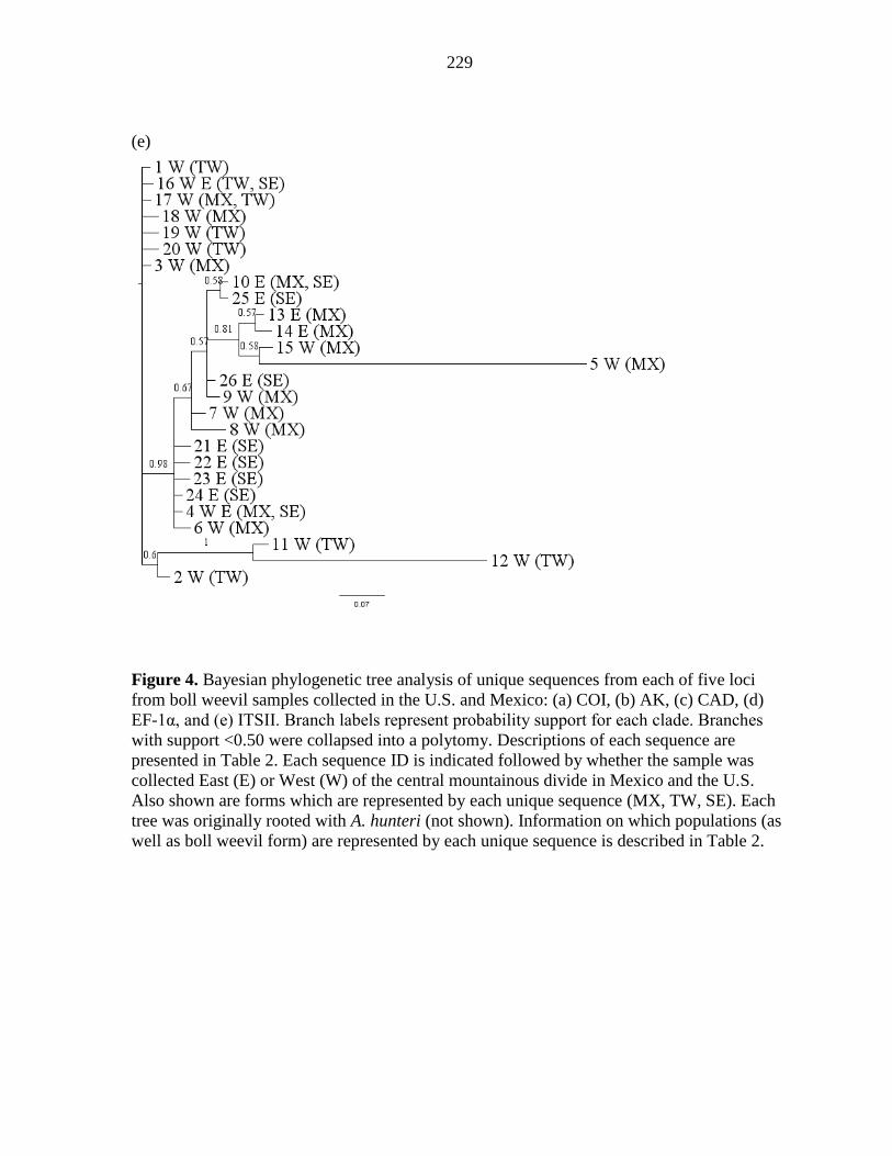
229

(e)

Figure 4. Bayesian phylogenetic tree analysis of unique sequences from each of five loci

from boll weevil samples collected in the U.S. and Mexico: (a) COI, (b) AK, (c) CAD, (d)

EF-1α, and (e) ITSII. Branch labels represent probability support for each clade. Branches

with support <0.50 were collapsed into a polytomy. Descriptions of each sequence are

presented in Table 2. Each sequence ID is indicated followed by whether the sample was

collected East (E) or West (W) of the central mountainous divide in Mexico and the U.S.

Also shown are forms which are represented by each unique sequence (MX, TW, SE). Each

tree was originally rooted with A. hunteri (not shown). Information on which populations (as

well as boll weevil form) are represented by each unique sequence is described in Table 2.

230

Table S1. Hierarchical AMOVA analyses for each locus and combined loci (COI, AK, CAD,

and EF-1α) for each of four models tested (see Fig. 1): subspecies and 3 forms (Model 1),

East versus West division with distinct TW group (Model 2), 3 forms (Model 3), and East

versus West division (Model 4). Observed Partition of Variance

Locus Variance Component Df % total P Φ-Statistics

COI

Model1 Among Subspecies 1 ΦST 0% 1.000 -0.340

Among Forms within Subspecies 1 ΦFS 53% 0.010 0.532

Within Forms 117 ΦFT 47% 0.010 0.373

Model2 Among Regions (East versus West) 1 ΦRT 54% 0.010 0.544

Among Forms within Regions 1 ΦFR 4% 0.060 0.084

Within Forms 117 ΦFT 42% 0.010 0.582

Model 3 Among Forms 2 ΦFT 50% 0.010 0.498

Within Forms 117 50%

Model 4 Among Regions (East versus West) 1 ΦRT 57% 0.001 0.567

Among Populations within Regions 23 ΦFR 12% 0.001 0.269

Within Populations 95 ΦPT 32% 0.001 0.683

AK

Model1 Among Subspecies 1 ΦST 0% 0.570 -0.021

Among Forms within Subspecies 1 ΦFS 6% 0.030 0.064

Within Forms 49 ΦFT 94% 0.290 0.044

Model2 Among Regions (East versus West) 1 ΦRT 0% 0.660 -0.018

Among Forms within Regions 1 ΦFR 9% 0.170 0.088

Within Forms 49 ΦFT 91% 0.010 0.071

Model 3 Among Forms 2 ΦFT 6% 0.059 0.032

Within Forms 49 94%

Model 4 Among Regions (East versus West) 1 ΦRT 4% 0.024 0.041

Among Populations within Regions 18 ΦFR 28% 0.001 0.287

Within Populations 32 ΦPT 68% 0.001 0.317

CAD

Model1 Among Subspecies 1 ΦST 0% 1.000 -0.547

Among Forms within Subspecies 1 ΦFS 52% 0.010 0.519

Within Forms 79 ΦFT 48% 0.010 0.256

Model2 Among Regions (East versus West) 1 ΦRT 38% 0.010 0.381

Among Forms within Regions 1 ΦFR 7% 0.030 0.116

Within Forms 79 ΦFT 55% 0.010 0.453

Model 3 Among Forms 2 ΦFT 47% 0.001 0.470

Within Forms 79 53%

Model 4 Among Regions (East versus West) 1 ΦRT 43% 0.001 0.428

Among Populations within Regions 17 ΦFR 15% 0.001 0.260

231

Table S1 Continued Observed Partition of Variance

Locus Variance Component Df % total P Φ-Statistics

Within Populations 63 ΦPT 42% 0.001 0.577

EF-1α

Model 1 Among Subspecies 1 ΦST 0% 0.990 -0.079

Among Forms within Subspecies 1 ΦFS 18% 0.010 0.181

Within Forms 42 ΦFT 82% 0.020 0.117

Model 2 Among Regions (East versus West) 1 ΦRT 15% 0.010 0.152

Among Forms within Regions 1 ΦFR 6% 0.030 0.076

Within Forms 42 ΦFT 78% 0.010 0.217

Model 3 Among Forms 2 ΦFT 15% 0.010 0.153

Within Forms 42 85%

Model 4 Among Regions (East versus West) 1 ΦRT 19% 0.001 0.190

Among Populations within Regions 12 ΦFR 9% 0.080 0.115

Within Populations 31 ΦPT 72% 0.001 0.283

Combined

Model 1 Among Subspecies 1 ΦST 1% 0.292 0.008

Among Forms within Subspecies 1 ΦFS 1% 0.146 0.010

Within Forms 129 ΦFT 98% 0.208 0.018

Model 2 Among Regions (East versus West) 1 ΦRT 0% 0.834 -0.027

Among Forms within Regions 1 ΦFR 4% 0.135 0.036

Within Forms 129 ΦFT 96% 0.156 0.010

Model 3 Among Forms 2 ΦFT 1% 0.163 0.012

Within Forms 129 99%

Model 4 Among Regions (East versus West) 1 ΦRT 1% 0.229 0.005

Among Populations within Regions 130 99%

ITSII

Model 1 Among Subspecies 1 ΦST 26% 0.010 0.257

Among Forms within Subspecies 1 ΦFS 15% 0.010 0.202

Within Forms 72 ΦFT 59% 0.001 0.407

Model 2 Among Regions (East versus West) 1 ΦRT 0% 0.880 -0.033

Among Forms within Regions 1 ΦFR 37% 0.010 0.371

Within Forms 72 ΦFT 63% 0.010 0.350

Model 3 Among Forms 2 ΦFT 29% 0.001 0.292

Within Forms 72 71%

Model 4 Among Regions (East versus West) 1 ΦRT 26% 0.010 0.264

Within Populations 73 74%

232

Table S2. Analysis of Molecular Variance to assess among-host species differentiation of

boll weevil populations in the Sonoran Desert for each locus. Sources of variance are for

among and within boll weevil host species (G. davidsonii, G. thurberi, G. turneri, G.

hirsutum, G. aridum). Indicated are degrees of freedom (Df), % of total genetic variance, the

P-value associated with ΦHT and Differentiation among host species (ΦHT).

Observed Partition of Variance

Locus Variance Component Df

%

total P ΦHT

CAD

Among Pops 4 5 0.033 0.051

Within Pops 49

AK

Among Pops 4 14 0.050 0.141

Within Pops 25

EF-1α

Among Pops 4 16 0.019 0.157

Within Pops 23

COI

Among Pops 4 23 0.001 0.231

Within Pops 65

Table S3. Locus-specific statistics for A. grandis populations in Mexico and the U.S. Shown are number of sequences (N),

sequence length, number of polymorphic sites, number of informative sites, number of unique sequences, haplotype diversity,

nucleotide diversity, and P-values associated with theta (4Nμ) for West (θW) and East (θE) Regions. θW and θE were corrected for

allelic diversity using Hedrick’s (2005) correction for GST.

Locus N Sequence # Polymorphic # Informative # Sequences Sequence Nucleotide θW P θE P

Length Sites Sites Diversity Diversity

COI 117 506 62 59 49 0.986 0.02722 1.0544 <0.001 0.137 <0.001

AK 43 539 5 2 18 0.495 0.00404 0.023 <0.001 0.032 <0.001

CAD 75 276 17 6 21 0.962 0.01111 0.031 <0.001 0.074 <0.001

EF-1α 48 523 47 11 19 0.929 0.01283 0.677 <0.001 0.003 <0.001

ITSII 75 642 137 6 26 0.807 0.01683 0.095 <0.001 0.022 <0.001

240 233

234

CHAPTER 7. General Conclusions

Summary

We investigated the marked variation in plant defense observed within and among

populations of Gossypium davidsonii. We explored the degree to which that variation is

attributable to environmental conditions, previously recognized to affect plant defenses. In

particular, we determined that a large proportion of variation was consistently attributable to

among population genetic differentiation, indicating the observed phenotypes probably are

under genetic control. Though we detected significant main effects of environment on some

measured traits, the phenotypic differences between environmental treatments were not

biologically relevant. Overall, minimal plasticity in defense traits derived from extreme

environmental conditions, producing considerably less variation than observed in nature.

Having assessed the effects of simulated herbivory on measured defense phenotypes,

we explored how these phenotypes affected levels of herbivory in the field. We found

inconsistencies among studied populations as to relative importance of measured defense

traits, geography, and genetic dissimilarity on herbivory responses by insect herbivores;

however, we documented trends in defense trait tradeoffs in two northern and two southern

populations and fine scale genetic structuring within three of those four sites. Observed

similarities between populations in the north and south of the species’ range may result from

similarity in herbivore communities on the wild cotton host in those areas.

Because variation in defense traits observed in the wild is likely not attributable to

plastic responses to changing or differing environmental conditions, we quantified whether,

and the extent to which, defense traits were under natural selection. We estimated genetic

differentiation among populations using neutral genetic markers, FST, and an analogous

235

phenotypic statistic for differentiation among populations, PST, to determine the level and

direction of selection on defense traits in 21 populations of G. davidsonii. While we found a

high level of genetic differentiation among populations in FST (FST = 0.182), we similarly

found high levels of differentiation in the observed phenotypes (PST Trichome = 0.312, PST

Leaf Gland = 0.570, PST Seed Gland = 0.644), which suggests divergent selection across the

range of G. davidsonii. We interpret disruptive selection as potentially being affected by

differences in insect herbivore communities on the cotton host across the species’ range.

We found genetic structuring within G. davidsonii populations within the southern

cape region of the Baja Peninsula and determined whether ancestral and contemporary gene

flow within A. grandis-associated populations of G. davidsonii and A. grandis were

symmetrical. High levels of genetic structure within G. davidsonii likely represents limited

ability of the plant to disperse long distances, though our detection of recent migrants from

several populations suggests either pollen dispersal from an un-identified pollinator or seed

dispersal, whereas genetic structuring within A. grandis populations may reflect a high

degree of adaptation to local ecotypes of G. davidsonii and the lack of detection of migrants

may be a result of poor host suitability across sites.

Lastly, we assessed the population genetic structure of the boll weevil in North

America on cultivated and wild cotton hosts. We reassessed classification of boll weevil

groups and determined the most parsimonious classification given the genetic data. These

data supported two well-differentiated groups: an eastern group comprising the Southeastern

form and the Mexican form east of the Sierra Madre Occidental, and a western group

comprising the thurberia form and the Mexican form west of this mountain range. This

arrangement contrasts with the traditional classification of boll weevils into Southeastern

236

(from G. hirsutum in the southeastern United States and northeastern Mexico), thurberia

(southern Arizona and northwestern Mexico), and Mexican (the remainder of Mexico and

Central America) forms. We also found little support for the classification of two subspecies,

A. g. grandis and A. g. thurberiae. Though traditional classification and subspecies status has

utility, classification based on regional differentiation should also be considered.

Future Research

Several additional questions would be valuable to address from this thesis work. In

particular, we found that defense traits may be under selection, but have not shown the

causes of selection. It would be important to investigate at a fine scale to determine how

defense phenotypes affect fitness. Additional years of sampling would likely determine

whether defense patterns do, indeed, have consequences on insect herbivory. Also, QTL

assessment of genes associated with defense traits would be helpful to determine the extent

of selection among populations in the wild.

Though we found genetic structure within A. grandis populations associated with G.

davidsonii and selection for foliar defenses within A. grandis- associated populations of G.

davidsonii, it is unclear how boll weevils influence plant defense trait variation. Studies of

inter-host population suitability may shed light on whether genetic structure among boll

weevil populations is attributable to host suitability. Likewise, while we found significant

effects of host species on genetic differentiation of boll weevils collected from western

Mexico, it is unclear whether host preference or identification is important for boll weevil

reproduction. Additional study on host preference and suitability will be needed to

understand populations of boll weevils on alternative cotton hosts in Mexico. Additional

237

geographic samples within regions of G. thurberi will also be needed to reassess the status of

the subspecies classification of A. g. thurberiae, as suggested by previous work.

238

APPENDIX. DNA Sequencing

Arginine Kinase

>ak.1 Arginine Kinase Unique Sequence 1

TACCCAATTGGTTGGGCAGAAAGTAAGGAAACCAAGCCTGTCATTATGAGAGAA

AGGAATGCGCTTCTCGATGTCATTGACAGCAGTTACAAGACGACGGTAGACTTCT

CCCAAGTCTCCTCCCATTTGCATGGAAATAATACGAAGGTGATCTTCCTCGTTAC

ACCAAACCAAGAATGTTTTGTTGTCGTTGTGGTAGATACCACGACCAGTTGGCCA

GAAGCGGCAAGCATTGGCAGCTTGCAAGAACCTGTCACCTTCCTTGAACAAGAA

GTGATCATCGATCAGCTTTTGCTGAACTTCCTTGCTCATTCCAGTCAATGGGTAG

AATGTACCCTTGAGTTCTCCTTCAAGCCCAGAAAGAGTGGAGGAAACTTTCTGTT

CCATCTCTTTGTATTGCTCTTCAGTCAAGCAAGGATTGAATGGGTATCCTTCCATA

GACCTTCCGCATCTTACACGGGTGGAGACAACATATTCACCAGTGGGGTCGAGG

TTGCCGAATACGTTGACATCACCCCAGTTCTTGGGGGGGTGTTTGT

>ak.10 Arginine Kinase Unique Sequence 10

TACCCAAGTTGGTTGGGCAGAAAGTAAGGAAACCAAGCCTGTCATTATGAGAGA

AAGGAATGCGCTTCTTGATGTCATTGACAGCAGTTACAAGACGACGGTAGACTT

CTCCCAAGTCTCCTCCCATTTGCATGGAAATAATACGAAGGTGATTTTCCTCGTT

ACACCAAACTAAGAATGTTTTGTTGTCGTTGTGGTAGATACCACGACCAGTTGGC

CAGAAGCGGCAAGCATTGGCAGCTTGCAAGAACCTGTCACCTTCCTTGAACAAG

AAGTGATCATCGATCAGCTTTTGCTGAACTTCCTTGCTCATTCCAGTCAATGGGT

AGAATGTACCCTTGAGTTCTCCTTCAAGCCCAGAAAGAGTGGAGGAAACTTTCTG

TTCCATCTTTTTGTATTGCTTTTCAGTCAAGCAAGGATTGAATGGGTATCCTTCCA

TAGACCTTCCGCATCTTACACGGGTGGAGACAACATATTCACCAGTGGGGTCGA

GGTTGCCGAATACGTTGACATCACCCCAGTTTTTGGGGGGGTGTTTGT

>ak.11 Arginine Kinase Unique Sequence 11

TACCCAAGTTGGTTGGGCAGAAAGTAAGGAAACCAAGCCTGTCATTATGAGAGA

AAGGAATGCGCTTCTCGATGTCATTGACAGCAGTTACAAGACGACGGTAGACTT

CTCCCAAGTCTCCTCCCATTTGCATGGAAATAATACGAAGGTGATCTTCCTCGTT

ACACCAAACCAAGAATGTTTTGTTGTCGTTGTGGTAGATACCACGACCAGTTGGC

CAGAAGCGGCAAGCATTGGCAGCTTGCAAGAACCTGTCACCTTCCTTGAACAAG

AAGTGATCATCGATCAGCTTTTGCTGAACTTCCTTGCTCATTCCAGTCAATGGGT

AGAATGTACCCTTGAGTTCTCCTTCAAGCCCAGAAAGAGTGGAGGAAACTTTCTG

TTCCATCTCTTTGTATTGCTCTTCAGTCAAGCAAGGATTGAATGGGTATCCTTCCA

TAGACCTTCCGCATCTTACACGGGTGGAGACAACATATTCACCAGTGGGGTCGA

GGTTGCCGAATACGTTGACATCACCCCAGTTCTTGGGGGGGTGTTTGT

>ak.12 Arginine Kinase Unique Sequence 12

TACCCAAGTTGGTTGGGCAGAAAGTAAGGAAACCAAGCCTGTCATTATGAGAGA

AAGGAATGCGCTTCTCGATGTCATTGACAGCAGTTACAAGACGACGGTAGACTT

CTCCCAAGTCTCCTCCCATTTGCATGGAAATAATACGAAGGTGATCTTCCTCGTT

ACACCAAACCAAGAATGTTTTGTTGTCGTTGTGGTAGATACCACGACCAGTTGGC

239

CAGAAGCGGCAAGCATTGGCAGCTTGCAAGAACCTGTCACCTTCCTTGAACAAG

AAGTGATCATCGATCAGCTTTTGCTGAACTTCCTTGCTCATTCCAGTCAATGGGT

AGAATGTACCCTTGAGTTCTCCTTCAAGCCCAGAAAGAGGGGAGGAAACTTTCT

GTTCCATCTCTTTGTATTGCTCTTCAGTCAAGCAAGGATTGAATGGGTATCCTTCC

ATAGACCTTCTGCATCTTACACGGGTGGAGACAACATATTCACCAGTGGGGTCG

AGGTTGCCGAATACGTTGACATCACCCCAGTTCTTGGGGGGGTGTTTGT

>ak.13 Arginine Kinase Unique Sequence 13

TACCCAAGTTGGTTGGGCAGAAAGTAAGGAAACCAAGCCTGCTCATTATGAGAG

AAAGGAATGCGCTTCTCGATGTCATTGACAGCAGTTACAAGACGACGGTAGACT

TCTCCCAAGTCTCCTCCCATTTGCATGGAAATGATACGAAGGTGATCTTCCTCGT

TACACCAAACCAAGAATGTTTTGTTGTCGTTGTGGTAGATACCACGACCAGTTGG

CCAGAAGCGGCAAGCATTGGCAGCTTGCAAGAACCTGTCACCTTCCTTGAACAA

GAAGTGATCATCGATCAGCTTTTGCTGAACTTCCTTGCTCATTCCAGTCAATGGG

TAGAATGTACCCTTGAGTTCTCCTTCAAGCCCAGAAAGAGTGGAGGAAACTTTCT

GTTCCATCTCTTTGTATTGCTCTTCAGTCAAGCAAGGATTGAATGGGTATCCTTCC

ATAGACCTTCCGCATCTTACACGGGTGGAGACAACATATTCACCAGTGGGGTCG

AGGTTGCCGAATACGTTGACATCACCCCAGTTCTTGGGGGGGTGTTTGT

>ak.14 Arginine Kinase Unique Sequence 14

TACCCAAGTTGGTTGGGCAGAAAGTAAGGAAACCAAGCCTGTCATTATGAGAGA

AAGGAATGCGCTTCTCGATGTCATTGACAGCAGTTACAAGACGACGGTAGACTT

CTCCCAAGTCTCCTCCCATTTGCATGGAAATAATACGAAGGTGATCTTCCTCGTT

ACACCAAACCAAGAATGTTTTTGTTGTCGTTGTGGTAGATACCACGACCAGTTGG

CCAGAAGCGGCAAGCATTGGCAGCTTGCAAGAACCTGTCACCTTCCTTGAACAA

GAAGTGATCATCGATCAGCTTTTGCTGAACTTCCTTGCTCATTCCAGTCAATGGG

TAGAATGTACCCTTGAGTTCTCCTTCAAGCCCAGAAAGAGTGGAGGAAACTTTCT

GTTCCATCTCTTTGTATTGCTCTTCAGTCAAGCAAGGATTGAATGGGTATCCTTCC

ATAGACCTTCCGCATCTTACACGGGTGGAGACAACATATTCACCAGTGGGGTCG

AGGTAGCCGAATACGTTGACATCACCCCAGTTCTTGGGGGGGTGTTTGT

>ak.15 Arginine Kinase Unique Sequence 15

TACCCAAGTTGGTTGGGCAGAAAGTAAGGAAACCAAGCCTGTCATTATGAGAGA

AAGGAATGCGCTTCTCGATGTCATTGACAGCAGTTACAAGACGACGGTAGACTT

CTCCCAAGTCTCCTCCCATTTGCATGGAAATAATAAGAAGGTGATTTTCCTCGTT

ACACCAAACCAAGAATGTTTTGTTGTTGTTGTGGTAGATACCACGACCAGTTGGC

CAGAAGCGGCAAGCATTGGCAGCTTGCAAGAACCTGTCACCTTCCTTGAACAAG

AAGTGATCATCGATCAGCTTTTGCTGAACTTCCTTGCTCATTCCAGTCAATGGGT

AGAATGTACCCTTGAGTTCTCCTTCAAGCCCAGAAAGAGTGGAGGAAACTTTCTG

TTCCATCTCTTTGTATTGCTTTTCAGTCAAGCAAGGATTGAATGGGTATCCTTCCA

TAGACCTTCCGCATCTTACACGGGTGGAGACAACATATTCACCAGTGGGGTCGA

GGTTGCCGAATACGTTGACATCACCCCAgttcttgggggggtgtttgt

240

>ak.16 Arginine Kinase Unique Sequence 16

TACCCAAGTTGGTTGGGCAGAAAGTAAGGAAACCAAGCCTGTCATTATGAGAGA

AAGGAATGCGCTTCTCGATGTCATTGACAGCAGTTACAAGACGACGGTAGACTT

CTCCCAAGTCTCCTCCCATTTGCATGGAAATAATACGAAGGTGATCTTCCTCGTT

ACACCAAACCAAGAATGTTTTGTTGTCGTTGTGGTAGATACCACGACCAGTTGGC

CAGAAGCGGCAAGCATTGGCAGCTTGCAAGAACCTGTCACCTTCCTTGAACAAG

AAGTGATCATCGATCAGCTTTTGCTGAACTTCCTTGCTCATTCCAGTCAATGGGT

AGAATGTACCCTTGAGTTCTCCTTCAAGCCCAGAAAGAGTGGAGGAAACTTTCTG

TTCCATCTCTTTGTATTGCTTTTCAGTCAAGCAAGGATTGAATGGGTATCCTTCCA

TAGACCTTCCGCATTTTACACGGGTGGAGACAACATATTCACCAGTGGGGTCGA

GGTTGCCGAATACGTTGACATCACCCCAGTTCTTGGGGGGGTGTTTGT

>ak.17 Arginine Kinase Unique Sequence 17

TACCCAAGTTGGTTGGGCAGAAAGTAAGGAAACCAAGCCTGTCATTATGAGAGA

AAGGAATGCGCTTCTCGATGTCATTGACAGCAGTTACAAGACGACGGTAGACTT

CTCCCAAGTCTCCTCCCATTTGCATGGAAATAATACGAAGGTGATCTTCCTCGTT

ACACCAAACCAAGAATGTTTTGTTGTCGTTGTGGTAGATACCACGACCAGTTGGC

CAGAAGCGGCAAGCATTGGCAGCTTGCAAGAACCTGTCACCTTCCTTGAACAAG

AAGTGATCATCGATCAGCTTTTGCTGAACTTCCTTGCTCATTCCAGTCAATGGGT

AGAATGTACCCTTGAGTTCTCCTTCAAGCCCAGAAAGAGTGGAGGAAACTTTCTG

TTCCATCTCTTTGTATTGCTCTTCAGTCAAGCAAGGATTGAATGGGTATCCTTCCA

TAGACCTTCTGCATTTTACACGGGTGGAGACAACAAATTCACCAATGGGGTCGA

GGTTGCCGAATACGTTGACATCACCCCAGTTCTTGGGGGGGTGTTTGT

>ak.18 Arginine Kinase Unique Sequence 18

TACCCAAGTTGGGTTGGGCAGAAAGTAAGGAAACCAAGCCTGTCATTATGAGAG

AAAGGAATGCGCTTCTCGATGTCATTGACAGCAGTTACAAGACGACGGTAGACT

TCTCCCAAGTCTCCTCCCATTTGCATGGAAATAATACGAAGGTGATCTTCCTCGT

TACACCAAACCAAGAATGTTTTGTTGTCGTTGTGGTAGATACCACGACCAGTTGG

CCAGAAGCGGCAAGCATTGGCAGCTTGCAAGAACCTGTCACCTTCCTTGAACAA

GAAGTGATCATCGATCAGCTTTTGCTGAACTTCCTTGCTCATTCCAGTCAATGGG

TAGAATGTACCCTTGAGTTCTCCTTCAAGCCCAGAAAGAGTGGAGGAAACTTTCT

GTTCCATCTCTTTGTATTGCTCTTCAGTCAAGCAAGGATTGAATGGGTATCCTTCC

ATAGACCTTCCGCATCTTACACGGGTGGAGACAACATATTCACCAGTGGGGTCG

AGGTTGCCGAATACGTTGACATCACCCCAGTTCTTGGGGGGGTGTTTGT

>ak.19 Arginine Kinase Unique Sequence 19

TACCCAAGTTGGGTTGGGCAGAAAGTAAGGAAACCAAGCCTGTCATTATGAGAG

AAAGGAATGCGCTTCTCGATGTCATTGACAGCAGTTACAAGACGACGGTAGACT

TCTCCCAAGTCTCCTCCCATTTGCATGGAAATAATACGAAGGTGATCTTCCTCGT

TACACCAAACCAAGAATGTTTTGTTGTCGTTGTGGTAGATACCACGACCAGTTGG

CCAGAAGCGGCAAGCATTGGCAGCTTGCAAGAACCTGTCACCTTCCTTGAACAA

GAAGTGATCATCGATCAGCTTTTGCTGAACTTCCTTGCTCATTCCAGTCAATGGG

TAGAATGTACCCTTGAGTTCTCCTTCAAGCCCAGAAAGAGTGGAGGAAACTTTCT

GTTCCATCTCTTTGTATTGCTCTTCAGTCAAGCAAGGATTGAATGGGTATCCTTCC

241

ATAGACCTTCCGCATCTTACACGGGTGGAGACAACATATTCACCAGTGGGGTCG

AGGTTGCCGAATACGTTGACATCACCCCAGTTCTTGGGGGGGTGTTTGT

>ak.2 Arginine Kinase Unique Sequence 2

TACCCAATTGGTTGGGCAGAAAGTAAGGAAACCAAGCCTGTCATTATGAGAGAA

AGGAATGCGCTTCTCGATGTCATTGACAGCAGTTACAAGACGACGGTAGACTTCT

CCCAAGTCTCCTCCCATTTGCATGGAAATAATACGAAGGTGATCTTCCTCGTTAC

ACCAAACCAAGAATGTTTTGTTGTCGTTGTGGTAGATACCACGACCAGTTGGCCA

GAAGCGGCAAGCATTGGCAGCTTGCAAGAACCTGTCACCTTCCTTGAACAAGAA

GTGATCATCGATCAGCTTTTGCTGAACTTCCTTGCTCATTCCAGTCAATGGGTAG

AATGTACCCTTGAGTTCTCCTTCAAGCCCAGAAAGAGTGGAGGAAACTTTCTGTT

CCATCTCTTTGTATTGCTCTTCAGTCAAGCAAGGATTGAATGGGTATCCTTCCATA

GACCTTCCGCATCTTACACGGGTGGAGACAACATATTCACCAGTGGGGTCGAGG

TTGCCGAATACGTTGACATCACCCCAGTTCTTGGGGGGGTGTTTGT

>ak.20 Arginine Kinase Unique Sequence 20

TACCCAAGTTGGTTGGGCAGAAAGTAAGGAAACCAAGCCTGTCATTATGAGAGA

AAGGAATGCGCTTCTCGATGTCATTGACAGCAGTTACAAGACGACGGTAGACTT

CTCCCAAGTCTCCTCCCATTTGCATGGAAATAATACGAAGGTGATCTTCCTCGTT

ACACCAAACCAAGAATGTTTTGTTGTCGTTGTGGTAGATACCACGACCAGTTGGC

CAGAAGCGGCAAGCATTGGCAGCTTGCAAGAACCTGTCACCTTCCTTGAACAAG

AAGTGATCATCGATCAGCTTTTGCTGAACTTCCTTGCTCATTCCAGTCAATGGGT

AGAATGTACCCTTGAGTTCTCCTTCAAGCCCAGAAAGAGTGGAGGAAACTTTCTG

TTCCATCTCTTTGTATTGCTCTTCAGTCAAGCAAGGATTGAATGGGTATCCTTCCA

TAGACCTTCCGCATCTTACACGGGTGGAGACAACATATTCACCAGTGGGGTCGA

GGTTGCCGAATACGTTGACATCACCCCAGTTCTTGGGGGGGTGTTTGT

>ak.21 Arginine Kinase Unique Sequence 21

TACCCAAGTTGGTTGGGCAGAAAGTAAGGAAACCAAGCCTGTCATTATGAGAGA

AAGGAATGCGCTTCTCGATGTCATTGACAGCAGTTACAAGACGACGGTAGACTT

CTCCCAAGTCTCCTCCCATTTGCATGGAAATAATACGAAGGTGATCTTCCTCGTT

ACACCAAACCAAGAATGTTTTGTTGTCGTTGTGGTAGATACCACGACCAGTTGGC

CAGAAGCGGCAAGCATTGGCAGCTTGCAAGAACCTGTCACCTTCCTTGAACAAG

AAGTGATCATCGATCAGCTTTTGCTGAACTTCCTTGCTCATTCCAGTCAATGGGT

AGAATGTACCCTTGAGTTCTCCTTCAAGCCCAGAAAGAGTGGAGGAAACTTTCTG

TTCCATCTCTTTGTATTGCTCTTCAGTCAAGCAAGGATTGAATGGGTATCCTTCCA

TAGACCTTCCGCATCTTACACGGGTGGAGACAACATATTCACCAGTGGGGTCGA

GGTTGCCGAATACGTTGACATCACCCCAGTTCTTGGGGGGGTGTTTGT

>ak.22 Arginine Kinase Unique Sequence 22

TACCCAAGTTGGTTGGGCAGAAAGTAAGGAAACCAAGCCTGTCATTATGAGAGA

AAGGAATGCGCTTCTCGATGTCATTGACAGCAGTTACAAGACGACGGTAGACTT

CTCCCAAGTCTCCTCCCATTTGCATGGAAATGATACGAAGGTGATCTTCCTCGTT

ACACCAAACCAAGAATGTTTTGTTGTCGTTGTGGTAGATACCACGACCAGTTGGC

CAGAAGCGGCAAGCATTGGCAGCTTGCAAGAACCTGTCACCTTCCTTGAACAAG

242

AAGTGATCATCGATCAGCTTTTGCTGAACTTCCTTGCTCATTCCAGTCAATGGGT

AGAATGTACCCTTGAGTTCTCCTTCAAGCCCAGAAAGAGTGGAGGAAACTTTCTG

TTCCATCTCTTTGTATTGCTCTTCAGTCAAGCAAGGATTGAATGGGTATCCTTCCA

TAGACCTTCCGCATCTTACACGGGTGGAGACAACATATTCACCAGTGGGGTCGA

GGTTGCCGAATACGTTGACATCACCCCAGTTCTTGGGGGGGTGTTTGT

>ak.23 Arginine Kinase Unique Sequence 23

TACCCAAGTTGGGTTGGGCAGAAAGTAAGGAAACCAAGCCTGTCATTATGAGAG

AAAGGAATGCGCTTCTCGATGTCATTGACAGCAGTTACAAGACGACGGTAGACT

TCTCCCAAGTCTCCTCCCATTTGCATGGAAATAATACGAAGGTGATCTTCCTCGT

TACACCAAACCAAGAATGTTTTGTTGTCGTTGTGGTAGATACCACGACCAGTTGG

CCAGAAGCGGCAAGCATTGGCAGCTTGCAAGAACCTGTCACCTTCCTTGAACAA

GAAGTGATCATCGATCAGCTTTTGCTGAACTTCCTTGCTCATTCCAGTCAATGGG

TAGAATGTACCCTTGAGTTCTCCTTCAAGCCCAGAAAGAGTGGAGGAAACTTTCT

GTTCCATCTCTTTGTATTGCTCTTCAGTCAAGCAAGGATTGAATGGGTATCCTTCC

ATAGACCTTCCGCATCTTACACGGGTGGAGACAACATATTCACCAGTGGGGTCG

AGGTTGCCGAATACGTTGACATCACCCCAGTTCTTGGGGGGGTGTTTGT

>ak.3 Arginine Kinase Unique Sequence 3

TTACCCAATTGGTTGGGCAGAAAGTAAGGAAACCAAGCCTGTCATTATGAGAGA

AAGGAATGCGCTTCTCGATGTCATTGACAGCAGTTACAAGACGACGGTAGACTT

CTCCCAAGTCTCCTCCCATTTGCATGGAAATAATACGAAGGTGATCTTCCTCGTT

ACACCAAACTAAGAATGTTTTGTTGTCGTTGTGGTAGATACCACGACCAGTTGGC

CAGAAGCGGCAAGCATTGGCAGCTTGCAAGAACCTGTCACCTTCCTTGAACAAG

AAGTGATCATCGATCAGCTTTTGCTGAACTTCCTTGCTCATTCCAGTCAATGGGT

AGAATGTACCCTTGAGTTCTCCTTCAAGCCCAGAAAGAGTGGAGGAAACTTTCTG

TTCCATCTCTTTGTATTGCTCTTCAGTCAAGCAAGGATTGAATGGGTATCCTTCCA

TAGACCTTCCGCATCTTACACGGGTGGAGACAACATATTCACCAGTGGGGTCGA

GGTTGCCGAATACGTTGACATCACCCCAGTTCTTGGGGGGGTGTTTGT

>ak.4 Arginine Kinase Unique Sequence 4

AAGGTGATCTTCCTCGTTACACCAAACTAAGAATGTTTTGTTGTCGTTGTGGTAG

ATACCACGACCAGTTGGCCAGAAGCGGCAAGCATTGGCAGCTTGCAAGAACCTG

TCACCTTCCTTGAACAAGAAGTGATCATCGATCAGCTTTTGCTGAACTTCCTTGCT

CATTCCAGTCAATGGGTAGAATGTACCCTTGAGTTCTCCTTCAAGCCCAGAAAGA

GTGGAGGAAACTTTCTGTTCCATCTCTTTGTATTGCTCTTCAGTCAAGCAAGGATT

GAATGGGTATCCTTCCATAGACCTTCCGCATTTTACACGGGTGGAGACAACATAT

TCACCAGTGGGGTCGAGGTTGCCGAATACGTTGACATCACCCCAGTTCTTGGGGG

GGTGTTTGT

>ak.5 Arginine Kinase Unique Sequence 5

AAGAAGTGATCATCGATCAGCTTTTGCTGAACTTCCTTGCTCATTCCAGTCAATG

GGTAGAATGTACCCTTGAGTTCTCCTTCAAGCCCAGAAAGAGTGGAGGAAACTT

TCTGTTCCATCTCTTTGTATTGCTCTTCAGTCAAGCAAGGATTGAATGGGTATCCT

243

TCCATAGACCTTCCGCATCTTACACGGGTGGAGACAACATATTCACCAGTGGGGT

GAGGTTACCGAATACGTTGACATCACCCCAGTTCTTGGGGGGGGGTTGGT

>ak.6 Arginine Kinase Unique Sequence 6

TACCCAAGTTGGTTGGGCAGAAAGTAAGGAAACCAAGCCTGTCATTATGAGAGA

AAGGAATGCGCTTCTCGATGTCATTGACAGCAGTTACAAGACGACGGTAGACTT

CTCCCAAGTCTCCTCCCATTTGCGATGGAAATAATACGAAGGTGATCTTCCTCGT

TACACCAAACTAAGAATGTTTTGTTGTCGTTGTGGTAGATACCACGACCAGTTGG

CCAGAAGCGGCAAGCATTGGCAGCTTGCAAGAACCTGTCACCTTCCTTGAACAA

GAAGTGATCATCGATCAGCTTTTGCTGAACTTCCTTGCTCATTCCAGTCAATGGG

TAGAATGTACCCTTGAGTTTTCCTTCAAGCCCAGAAAGAGTGGAGGAAACTTTCT

GTTCCATCTCTTTGTATTGCTCTTCAGTCAAGCAAGGATTGAATGGGTATCCTTCC

ATAGACCTTCCGCATTTTACACGGGTGGAGACAACATATTCACCAGTGGGGTCG

AGGTTGCCGAATACGTTGACATCACCCCAGTTCTTGGGGGGGTGTTTGT

>ak.7 Arginine Kinase Unique Sequence 7

TACCCAAGTTGGGTTGGGCAGAAAGTAAGGAAACCAAGCCTGCTCATTATGAGA

GAAAGGAATGCGCTTCTCGATGTCATTGACAGCAGTTACAAGACGACGGTAGAC

TTCTCCCAAGTCTCCTCCCATTTGCATGGAAATAATACGAAGGTGATCTTCCTCG

TTACACCAAACTAAGAATGTTTTGTTGTCGTTGTGGTAGATACCACGACCAGTTG

GCCAGAAGCGGCAAGCATTGGCAGCTTGCAAGAACCTGTCACCTTCCTTGAACA

AGAAGTGATCATCGATCAGCTTTTGCTGAACTTCCTTGCTCATTCCAGTCAATGG

GTAGAATGTACCCTTGAGTTCTCCTTCAAGCCCAGAAAGAGTGGAGGAAACTTTC

TGTTCCATCTCTTTGTATTGCTCTTCAGTCAAGCAAGGATTGAATGGGTATCCTTC

CATAGACCTTCCGCATCTTACACGGGTGGAGACAACATATTCACCAGTGGGGTC

GAGGTTGCCGAATACGTTGACATCACCCCAGTTCTTGGGGGGGTGTTTGT

>ak.8 Arginine Kinase Unique Sequence 8

TACCCAAGTTGGTTGGGCAGAAAGTAAGGAAACCAAGCCTGTCATTATGAGAGA

AAGGAATGCGCTTCTCGATGTCATTGACAGCAGTTACAAGACGACGGTAGACTT

CTCCCAAGTCTCCTCCCATTTGCATGGAAATAATACGAAGGTGATCTTCCTCGTT

ACACCAAACTAAGAATGTTTTGTTGTCGTTGTGGTAGATACCACGACCAGTTGGC

CAGAAGCGGCAAGCATTGGCAGCTTGCAAGAACCTGTCACCTTCCTTGAACAAG

AAGTGATCATCGATCAGCTTTTGCTGAACTTCCTTGCTCATTCCAGTCAATGGGT

AGAATGTACCCTTGAGTTCTCCTTCAAGCCCAGAAAGAGTGGAGGAAACTTTCTG

TTCCATCTCTTTGTATTGCTCTTCAGTCAAGCAAGGATTGAATGGGTATCCTTCCA

TAGACCTTCCGCATCTTACACGGGTGGAGACAACATATTCACCAGTGGGGTCGA

GGTTGCCGAATACGTTGACATCACCCCAGTTCTTGGGGGGGTGTTTGT

>ak.9 Arginine Kinase Unique Sequence 9

TACCCAAGTTGGTTGGGCAGAAAGTAAGGAAACCAAGCCTGTCATTATGAGAGA

AAGGAATGCGCTTCTCGATGTCATTGACAGCAGTTACAAGACGACGGTAGACTT

CTCCCAAGTCTCCTCCCATTTGCATGGAAATAATACGAAGGTGATCTTCCTCGTT

ACACCAAACTAAGAATGTTTTGTTGTCGTTGTGGTAGATACCACGACCAGTTGGC

CAGAAGCGGCAAGCATTGGCAGCTTGCAAGAACCTGTCACCTTCCTTGAACAAG

244

AAGTGATCATCGATCAGCTTTTGCTGAACTTCCTTGCTCATTCCAGTCAATGGGT

AGAATGTACCCTTGAGTTCTCCTTCAAGCCCAGAAAGAGTGGAGGAAACTTTCTG

TTCCATCTCTTTGTATTGCTTTTCAGTCAAGCAAGGATTGAATGGGTATCCTTCCA

TAGACCTTCCGCATCTTACACGGGTGGAGACAACATATTCACCAGTGGGGTCGA

GGTTGCCGAATACGTTGACATCACCCCAGTTCTTGGGGGGGTGTTTGT

>ak.Ahunt Arginine Kinase Anthonomus hunteri

TACCCAAGTTGGTTGGGCAGAAAGTAAGGAAACCAAGCCTGTCATTATGAGAGA

AAGGAATGCGCTTCTCGATGTCATTGACAGCAGTTACAAGACGACGGTAGACTT

CTCCCAAGTCTCCTCCCATTTGCATGGAAATAATACGAAGGTGATCTTCCTCGTT

ACACCAAACCAAGAATGTTTTGTTGTCGTTGTGATAGATACCACGACCAGTTGGC

CAGAAACGGCAAGCATTGGCAGCTTGCAAGAATCTGTCACCTTCCTTGAACAAG

AAGTGATCATCGATCAGTTTTTGCTGAACTTCCTTGCTCATTCCAGTCAATGGGT

AGAATGTACCCTTGAGTTCTCCTTCAAGCCCAGAAAGAGTGGAGGAAACTTTCTG

TTCCATCTCTTTGTATTGCTCTTCAGTCAAGCAAGGATTGAATGGGTATCCTTCCA

TAGACCTTCCGCATCTTACACGGGTGGAGACAACATATTCACCAGTGGGGTCGA

GGTTGCCGAATACGTTGACATCACCCCAGTTCTTGGGGGGGT

CAD

>cad.1

TCCGGAAGTGGAGTGCCTAGGGCCAACTTGGCCGCCACGTAAGCCAACGGATAT

CCGGTCGCTTTGCTGGCCAACGCGGAACTTCTCGATAATCTCGCGTTCACTTCGA

TGATATAATACTCCTCCGAGTGCGGATTGAGGGCATACTGGATGTTACACTCGCC

CACCACCCCGAAGTGTCTTATCGCTTTAATCGCGGTGGTTCTGAGTAGGTTGTAC

TCGCGATTCGATAGGGTTTGACTGGGTGCGACCACGATCGATTCCCCCGTGTGGA

TACCTAAAGGGTCGACGTTCTCC

>cad.2

TCCGGAAGTGGAGTGCCTAGGGCCAACTTGGCCGCCACATAAGCCAACGGATAT

CCGGTCGCTTTGCTGGCCAACGCGGAACTTCTCGATAATCTCGCGTTCACTTCGA

TGATATAATACTCCTCCGAGTGCGGATTGAGGGCATACTGGATGTTACACTCGCC

CACCACCCCGAAGTGTCTTATCGCTTTAATCGCGGTGGTTCTGAGTAGGTTGTAC

TCGCGATTCGATAGGGTTTGACTGGGTGCGACCACGATCGATTCCCCCGTGTGGA

TACCTAAAGGGTCGACGTTCTCC

>cad.3

TCCGGAAGTGGAGTGCCTAGGGCCAACTTGGCCGCCACATAAGCCAACGGATAT

CCGGTCGCTTTGCTGGCCAACGCGGAACTTCTCGATAATCTCGCGTTCACTTCGA

TGATATAATACTCCTCCGAGTGCGGATTGAGGGCATACTGGATGTTACACTCGCC

CACCACCCCGAAGTGTCTTATCGCTTTATCGCGGGTGGTTCTGAGTAGGTTGTAC

TCGCGATTCGATAGGGTTTGACTGGGTGCGACCACGATCGATTCCCCCGTGTGGA

TACCTAAAGGGTCGACGTTCTCC

245

>cad.4

TCCGGAAGTGGAGTGCCTAGGGCCAACTTGGCCGCCACATAAGCCAACGGATAT

CCGGTCGCTTTGCTGGCCAACGCGGAACTTCTCGATAATCTCGCGTTCACTTCGA

TGATATAATACTCCTCCGAGTGCGGATTGAGGGCATACTGGATGTTACACTCGCC

CACCACCCCGAAGTGTCTTATCACTTTAATCGCGGTGGTTCTGAGTAGGTTGTAC

TCGCGATTCGATAGGGTTTGACTGGGTGCGACCACGATCGATTCCCCCGTGTGGA

TACCTAAAGGGTCGACGTTCTCC

>cad.5

TCCGGAAGTGGAGTGCCTAGGGCCAACTTGGCCGCCACATAAGCCAACGGATAT

CCGGTCGCTTTGCTGGCCAACGCGGAACTTCTCGATAATCTCGCGTTCACTTCGA

TGATATAATACTCCTCCGAGTGCGGATTGAGGGCGTACTGGATGTTACACTCGCC

CACCACCCCGAAGTGTCTTATCACTTTAATCGCGGTGGTTCTGAGTAGGTTGTAC

TCGCGATTCGATAGGGTTTGACTGGGTGCGACCACGATCGATTCCCCCGTGTGGA

TACCTAAAGGGTCGACGTTCTCC

>cad.6

TCCGGAAGTGGAGTGCCTAGGGACAACTTGGCCGCCACATAAGCCAACGGATAT

CCGGTCGCTTTGCTGGCCAACGCGGAACTTCTCGATAATCTCGCGTTCACTTCGA

TGATATAATACTCCTCCGAGTGCGGATTGAGGGCGTACTGGATGTTACACTCGCC

CACCACCCCGAAGTGTCTTATCACTTTAATCGCGGTGGTTCTGAGTAGGTTGTAC

TCGCGATTCGATAGGGTTTGACTGGGTGCGACCACGATCGATTCCCCCGTGTGGA

TACCTAAAGGGTCGACGTTCTCC

>cad.7

TCCGGAAGTGGAGTGCCTAGGGCCAACTTGGCCGCCACATAAGCCAACGGATAT

CCGGTCGCTTTGCTGGCCAACGCGGAACTTCTCGATAATCTCGCGTTCACTTCGA

TGATATAATACTCCTCCGAGTGCGGATTGAGGGCGTACTGGATGTTACACTCGCC

CACCACCCCGAAGTGTCTTATCACTTTAATCGCGGTGGTTCTGAGTAGGTTGTAC

TCGCGATTCGATAGTGTTTGACTGGGTGCGACCACGATCGATTCCCCCGTGTGGA

TACCTAAAGGGTCGACGTTCTCC

>cad.8

TCCGGAAGTGGAGTGCCTAGGGCCAACTTGGCCGCCACATAAGCCAACGGATAT

CCGGTCGCTTTGCTGGCCAACGCGGAACTTCTCGATAATCTCGCGTTCACCTCGA

TGATATAATACTCCTCCGAGTGCGGATTGAGGGCGTACTGGATGTTACACTCGCC

CACCACCCCGAAGTGTCTTATCACTTTAATCGCGGTGGTTCTGAGTAGGTTGTAC

TCGCGATTCGATAGGGTTTGACTGGGTGCGACCACGATCGATTCCCCCGTGTGGA

TACCTAAAGGGTCGACGTTCTCC

>cad.9

TCCGGAAGTGGAGTGCCTAGGGCCAACTTGGCCGCCACATAAGCCAACGGATAT

CCGGTCGCTTTGCTGGCCAACGCGGAACTTCTCGATAATCTCGCGTTCACCTCGA

TGATATAATACTCCTCCGAGTGCGGATTGAGGGCGTACTGGATGTTACACTCGCC

CACCACCCCGAAGTGTCTTATCGCTTTAATCGCGGTGGTTCTGAGTAGGTTGTAC

246

TCGCGATTCGATAGGGTTTGACTGGGTGCGACCACGATCGATTCCCCCGTGTGGA

TACCTAAAGGGTCGACGTTCTCC

>cad.10

TCCGGAAGTGGAGTGCCTAGGGCCAACTTGGCCGCCACGTAAGCCAACGGATAT

CCGGTCGCTTTGCTGGCCAACGCGGAACTTCTCGATAATCTCGCGTTCACTTCGA

TGATATAATACTCCTCCGAGTGCGGATTGAGGGCGTACTGGATGTTACACTCGCC

CACCACCCCGAAGTGTCTTATCACTTTAATCGCGGTGGTTCTGAGTAGGTTGTAC

TCGCGATTCGATAGGGTTTGACTGGGTGCGACCACGATCGATTCCCCCGTGTGGA

TACCTAAAGGGTCGACGTTCTCC

>cad.11

TCCGGAAGTGGAGTGCCTAGGGCCAACTTGGCCGCCACGTAAGCCAACGGATAT

CCGGTCGCTTTGCTGGCCAACGCGGAACTTCTCGATAATCTCGCGTTCACCTCGA

TGATATAATACTCCTCCGAGTGCGGATTGAGGGCGTACTGGATGTTACACTCGCC

CACCACCCCGAAGTGTCTTATCACTTTAATCGCGGTGGTTCTGAGTAGGTTGTAC

TCGCGATTCGATAGGGTTTGACTGGGTGCGACCACGATCGATTCCCCCGTGTGGA

TACCTAAAGGGTCGACGTTCTCC

>cad.12

TCCGGAAGTGGAGTGCCTAGGGCCAACTTGGCCGCCACATAAGCCAACGGATAT

CCGGTCGCTTTGCTGGCCAATGCGGAACTTCTCGATAATCTCGCGTTCACTTCGA

TGATATAATACTCCTCCGAGTGCGGATTGAGGGCGTACTGGATGTTACACTCGCC

CACCACCCCGAAGTGTCTTATCACTTTAATCGCGGTGGTTCTGAGTAGGTTGTAC

TCGCGATTCGATAGGGTTTGACTGGGTGCGACCACGATCGATTCCCCCGTGTGGA

TACCTAAAGGGTCGACGTTCTCC

>cad.13

TCCGGAAGTGGAGTGCCTAGGGCCAACTTGGCCGCCACATAAGCCAACGGATAT

CCGGTCGCTTTGCTGGCCATTGCGGAACTTCTCGATAATCTCGCGTTCACTTCGAT

GATATAATACTCCTCCGAGTGCGGATTGAGGGCGTACTGGATGTTACACTCGCCC

ACCACCCCGAAGTGTCTTATCACTTTAATCGCGGTGGTTCTGAGTAGGTTGTACT

CGCGATTCGATAGGGTTTGACTGGGTGCGACCACGATCGATTCCCCCGTGTGGAT

ACCTAAAGGGTCGACGTTCTCC

>cad.14

TCCGGAAGTGGAGTGCCTAGGGCCAACTTGGCCGCCACATAAGCCAACGGATAT

CCGGTCGCTTTGCTGGCCAATGCGGAACTTCTCGATAATCTCGCGTTCACTTCGA

TGATATAATACTCCTCCGAGTGCGGATTGAGGGCGTACTGGATGTTACACTCGCC

CACCACCCCGAAGTGTCTTATCACTTTAATCGCGGTGGTTCTGAGTAGGTTGTAC

TCGCGATTCGATAGGGTTTGACTGGGTGCGACCACAATCGATTCCCCCGTGTGGA

TACCTAAAGGGTCGACGTTCTCC

247

>cad.15

TCCGGAAGTGGAGTGCCTAGGGCCAACTTGGCCGCCACATAAGCCAACGGATAT

CCGGTCGCTTTGCTGGCCAATGCGGAACTTCTCGATAATCTCGCGTTCACTTCGA

TGATATAATACTCCTCCGAGTGCGGATTGAGGGCGTACTGGATGTTACACTCGCC

CACCACCCCGAAGTGTCTTATCACTTTAATCGCGGTGGTTCTGAGTAGGTTGTAC

TCGCGATTCGATAGGGTTTGACTGGGTGCGACCACGATCGATTCCCCCGTGTGGA

TACCTAACGGGTCGACGTTCTCC

>cad.16

TCCGGAAGTGGAGTGCCTAGGGCCAACTTGGCCGCCACATAAGCCAACGGATAT

CCGGTCGCTTTGCTGGCCAATGCGGAACTTCTCGATAATCTCGCGTTCACTTCGA

TGATATAATACTCCTCCGAGTGCGGATTGAGGGCGTACTGGATGTTACACTCGCC

CACCACCCCGAAGTGTCTTATCACTTTAATCGCGGTGGTTCTGAGTAGGTTGTAC

TCGTGATTCGATAGGGTTTGACTGGGTGCGACCACGATCGATTCCCCCGTGTGGA

TACCTAAAGGGTCGACGTTCTCC

>cad.17

TCCGGAAGTGGAGTGCCTAGGGCCAACTTGGCCGCCACATAAGCCAACGGATAT

CCGGTCGCTTTGCTGGCCTATGCGGAACTTCTCGATAATCTCGCGTTCACTTCGAT

GATATAATACTCCTCCGAGTGCGGATTGAGGGCGTACTGGATGTTACACTCGCCC

ACCACCCCGAAGTGTCTTATCACTTTAATCGCGGTGGTTCTGAGTAGGTTGTACT

CGCGATTCGATAGGGTTTGACTGGGTGCGACCACGATCGATTCCCCCGTGTGGAT

ACCTAAAGGGTCGACGTTCTCC

>cad.18

TCCGGAAGTGGAGTGCCTAGGGCCAACTTGGCCGCCACATAAGCCAACGGATAT

CCGGTCGCTTTGCTGGTCTATGCGGAACTTCTCGATAATCTCGCGTTCACTTCGAT

GATATAATACTCCTCCGAGTGCGGATTGAGGGCGTACTGGATGTTACACTCGCCC

ACCACCCCGAAGTGTCTTATCACTTTAATCGCGGTGGTTCTGAGTAGGTTGTACT

CGCGATTCGATAGGGTTTGACTGGGTGCGACCACGATCGATTCCCCCGTGTGGAT

ACCTAAAGGGTCGACGTTCTCC

>cad.19

TCCGGAAGTGGAGTGCCTAGGGCCAACTTGGCCGCCACATAAGCCAACGGATAT

CCGGTCGCTTTGCTGGCCTATGCGGAACTTCTCGATAATCTTGCGTTCACTTCGAT

GATATAATACTCCTCCGAGTGCGGATTGAGGGCGTACTGGATGTTACACTCGCCC

ACCACCCCGAAGTGTCTTATCACTTTAATCGCGGTGGTTCTGAGTAGGTTGTACT

CGTGATTCGATAGGGTTTGACTGGGTGCGACCACGATCGATTCCCCCGTGTGGAT

ACCTAAAGGGTCGACGTTCTCC

>cad.20

AACGGAAGTGGAGTGCCTAGGGCCAACTTGGCCGCCACATAAGCCAACGGATAT

CCGGTCGCTTTGCTGGCCAATGAAGAACTTCTCGATAATCTCGCGTTCACTTCGA

TGATATAATACTCCTCCGAGTGCGGATTGAGGGCGTACTGGATGTTACACTCGCC

CACCACCCCGAAGTGTCTTATCACTTTAATCGCGGTGGTTCTGAGTAGGTTGTAC

248

TCGCGATTCGATAGGGTTTGACTGGGTGCGACCACGATCGATTCCCCCGTGTGGA

TACCTAAAGGGTCGACGTTCTCC

>cad.21

TCCGGAAGTGGAGTGCCTAGGGCCAACTTGGCCGCCACATAAGCCAACGGATAT

CCGGTCGCTTTGCTGGCCGGTGCGGAACTTCTCGATAATCTCGCGTTCACTTCGA

TGATATAATACTCCTCCGAGTGCGGATTGAGGGCGTACTGGATGTTACACTCGCC

CACCACCCCGAAGTGTCTTATCACTTTAATCGCGGTGGTTCTGAGTAGGTTGTAC

TCGCGATTCGATAGGGTTTGACTGGGTGCGACCACGATCGATTCCCCCGTGTGGA

TACCTAAAGGGTCGACGTTCTCC

>cad.A.hunteri

TCCGGAAGTGGAGTGCCTAGGGCCAACTTGGCCGCCACATAAGCCAACGGATAT

CCGGTCGCTTTGCTTGCCAATGCGGAACTTCTCGATAATCTCGCGTTCACTTCGAT

GATATAATACTCCTCCGAGTGTGGATTGAGGGCGTACTGGATGTTACACTCGCCC

ACCACCCCGAAGTGTCTTATCACTTTAATCGCGGTGGTTCTGAGTAGGTTGTACT

CGCGATTCGATAGAGTTTGACTGGGTGCGACCACGATCGATTCCCCCGTGTGGAT

Elongation Factor 1 Alpha

>EF.1 Elongation Factor 1-alpha subunit Unique Sequence 1

ACTTTACTTCAGTGGACATGTTAGCTGGAGCAAACACTACTACAGTACCGGGTTT

AAGAATACCAGTTTCAACACGACCAACAGGTACCGTTCCAATACCTCCAATTTTG

TAAACATCCTGCAACAAACAAAATGTTAATAAAAAAAAACTATTTAAAAAATTT

AACAAACCTGAAGTGGAAGACGGAGGGCTTTGTCAGTAGGACGTGAAGGTGGA

AGGATGGCATCCAAAGCATCAATGAGTGTCTTGCCGTCAGCTTTGCCTTCTTTAC

GTTCAATGTTCCATCCCTTGAACCATGGCATCTTGGTGGAAGCTTCCAACATGTT

GTCTCCATGCCATCCAGAGATGGGCACGAATGCAACAGCAGCTGGATTGTAACC

AATCTTCTTGATGTATGAAGATACTTCTTTCTTGATTTCCTCAAAACGGCTTTCAC

TGTAGGGTGGTTCAGTGGAGTCCATCTTGTTGACACCAACGATAAGTTGTTTTAC

T

>EF.10 Elongation Factor 1-alpha subunit Unique Sequence 10

ACTTTACTTCAGTGGTAATGTTAGCTGGAGCAAACACTACTACAGTACCGGGTTT

AAGAATACCAGTTTCAACACGACCAACAGGTACCGTTCCAATACCTCCAATTTTG

TAAACATCCTGCAACAAACAAAATGTTAATAAAAAAAAACTATTTAAAAAATTT

AACAAACCTGAAGTGGAAGACGGAGGGCTTTGTCAGTAGGACGTGAAGGTGGA

AGGATGGCATCCAAAGCATCAATGAGTGTCTTGCCGTCAGCTTTGCCTTCTTTAC

GTTCAATGTTCCATCCCTTGAACCATGGCATCTTGGTGGAAGCTTCCAACATGTT

GTCTCCATGCCATCCAGAGATGGGCACGAATGCAACAGCAGCTGGATTGTAACC

AATCTTCTTGATGTATGAAGATACTTCTTTCTTGATTTCCTCAAAACGGCTTTCAC

TGTAGGGTGGTTCAGTGGAGTCCATCTTGTTGACACCAACGATAAGTTGTTTTAC

T

249

>EF.11 Elongation Factor 1-alpha subunit Unique Sequence 11

ACTTTACTTCAGTGGTAATGTTAGCTGGAGCAAACACTACTACAGTACCGGGTTT

AAGAATACCAGTTTCAACACGACCAACAGGTACCGTTCCGATACCTCCAATTTTG

TAAACATCCTGCAACAAACAAAATGTTAATAAAAAAAAACTATTTAAAAAATTT

AACAAACCTGAAGTGGAAGACGGAGGGCTTTGTCAGTAGGACGTGAAGGTGGA

AGGATGGCATCCAAAGCATCAATGAGTGTCTTGCCGTCAGCTTTGCCTTCTTTAC

GTTCAATGTTCCATCCCTTGAACCATGGCATCTTGGTGGAAGCTTCCAACATGTT

GTCTCCATGCCATCCAGAGATGGGCACGAATGCAACAGCAGCTGGATTGTAACC

AATCTTCTTGATGTATGAAGATACTTCTTTCTTGATTTCCTCAAAACGGCTTTCAC

TGTAGGGTGGTTCAGTGGAGTCCATCTTGTTGACACCAACGATAAGTTGTTTTAC

T

>EF.12 Elongation Factor 1-alpha subunit Unique Sequence 12

ACTTTACTTCAGTGGTAATGTTAGCTGGAGCAAACACTACTACAGTACCGGGTTT

AAGAATACCAGTTTCAACACGACCAACAGGTACCGTTCCAATACCTCCAATTTTG

TAAACATCCTGCAACAAACAAAATGTTAATAAAAAAAAACTATTTAAAAAATTT

AACAAACCTGAAGTGGAAGACGGAGGGCTTTGTCAGTAGGACGTGAAGGTGGA

AGGATGGCATCCAAAGCATCAATGAGTGTCTTGCCGTCACCTTTGCCTTCTTTAC

GTTCAATGTTCCATCCCTTGAACCATGGCATCTTGGTGGAAGCTTCCAACATGTT

GTCTCCATGCCATCAAGAGATGGGCACGAATGCAACAGCAGCTGGATTGTAACC

AATCTTCTTGATGTATGAAAATACTTCTTTCTTGATTTCCTCAAAACGGCTTTCAC

TGTAGGGTGGTTCAGTGGAGTCCATCTTGTTGACACCAACAATAAGTTGTTTTAC

T

>EF.13 Elongation Factor 1-alpha subunit Unique Sequence 13

ACTTTATTTCGGTGGTAAGGTTAGCTGGAGCAAACACTACTACAGTACCGGGTTT

AAAAATACCAGTTTCAACACGACCAACAGGTACCGTTCTAATACCTCCAATTTTG

TAAACATCCTGCAACAAACAAAATGTTAATAAAAAAAAACTAATTAAAAAAATT

TAACAAACCTGAAGTGGAAGACGGAGGGCTTTGTCAGTAGGACGTGAAGGTGGA

AGGATGGCATCCAAAGCATCAATGAGTGCCTTGCCCCCAGCTTTGCCTTCTTTAC

GTTCAAAGTTCCATCCCTTGAACCATGGCATCTTGGTGGAAGCTTCCAACATGTT

GTCTCCATGCCATCCAAAGATGGGCACGAATGCAACAGCAGCTGGATTGTAACC

AATCTTCTTGATGTATGAAAATACTTCTTTCTTGATTTCCTCAAAACGGCTTTCAC

TGTAGGGTGGTTCAGTGGAGTCCATCTTGTTGACACCAACGATAAATTGTTTTAC

T

>EF.14 Elongation Factor 1-alpha subunit Unique Sequence 14

ACTTTATTTCGGTGGTAAGGTTGGCGGGGGCAACCATTATTCCGGTACCGGGTTT

AGGATTCCCGGTTCCACCAGGACCACCGGGTCCGGTTCCAATCCTTCCAATTTGG

TAACCTTCCTGCACCAACCAAAAGGTTATTAAAAAAAAGTTATTTAAAAAATTTA

ACAAACCTGAAGTGGAAGACGGAGGGCTTTGTCAGTAGGACGTGAAGGTGGAA

GGATGGCATCCAAAGCATCAATGAGTGTCTTGCCGTCAGCTTTGCCTTCTTTACG

TTCAATGTTCCATCCCTTGAACCATGGCATCTTGGTGGAAGCTTCCAACATGTTG

TCTCCATGCCATCCAGAGATGGGCACGAATGCAACAGCAGCTGGATTGTAACCA

250

ATCTTCTTGATGTATGAAGATACTTCTTTCTTGATTTCCTCAAAACGGCTTTCACT

GTAGGGTGGTTCAGTGGAGTCCATCTTGTTGACACCAACGATAAGTTGTTTTACT

>EF.15 Elongation Factor 1-alpha subunit Unique Sequence 15

ACTTTACTTCAGTGGTAATGTTAGCTGGAGCAAACACTACTACAGTACCGGGTTT

AAGAATACCAGTTTCAACACGACCAACAGGTACCGTTCCAATACCTCCAATTTTG

TAAACATCCTGCAACAAACAAAATGTTAATAAAAAAAAACTATTTAAAAAATTT

AACAAACCTGAAGTGGAAGACGGAGGGCTTTTTCAGTAGGACATGAAGGTGGAA

GGATGGCACCCAAAACATCAATGAGTGTCTTGCCGCCACCTTTGCCTTCTTTACG

TTCAATGTTCCATCCCTTGAACCATGGCATCTTGGTGGAAACTTCCAACATGTTG

TCTCCATGCCATCAACAAATGGGCACGAATGCAACACCAGCTGGATTGTAACCA

ATCTTCTTGATGTATGAAGATACTTCTTTCTTGATTTCCTCAAAACGGCTTTCTCT

GTAAGGGGGTTCAGTGGACTCCATCTAGTTGACACCCACGATAAATTGTTTTACT

>EF.16 Elongation Factor 1-alpha subunit Unique Sequence 16

ACTTTACTTCAGTGGTAATGTTAGCTGGAGCAAACACTACTACAGTACCGGGTTT

AAGAATACCAGTTTCAACACGACCAACAGGTACCGTTCCAATACCTCCAATTTTT

TAAACATCCTGCAACAAACAAAATGTTAATAAAAAAAAACTATTTAAAAAAATT

TAACAAACCTGAAGTGGAAGACGGAGGGCTTTGTCAGTAGGACGTGAAGGTGGA

AGGATGGCATCCAAAGCATCAATGAGTGTCTTGCCGTCAGCTTTGCCTTCTTTAC

GTTCAATGTTCCGTCCCTTGAACCATGGCATCTTGGTGGAAGCTTCCAACATGTT

GTCTCCTTGCCATCCAGAGATGGGCACGAATGCACCGGCAGGTGGATTGTAACC

AATCTTCTTGATGTATGAAGATACTTCTTTCTTGATTTCCTCAAAACGGCTTTCAC

TGTAGGGTGGTTCAGTGGAGTCCATCTTGTTGACACCAACGATAAGTTGTTTTAC

T

>EF.17 Elongation Factor 1-alpha subunit Unique Sequence 17

ACTTTACTTCAGTGGTAATGTTAGCTGGAGCAAACACTACTACAGTACCGGGTTT

AAGAATACCAGTTTCAACACGACCAACAGGTACCGTTCCAATACCTCCAATTTTG

TAAACATCCTGCAACAAACAAAATGTTAATAAAAAAAAACTAATTAAAAAAATT

TAACAAACCTGAAGTGGAAGACGGAGGGCTTTGTCAGTAGGACGTGAAGGTGGA

AGGATGGCATCCAAAGCATCAATGAGTGTCTTGCCGTCAGCTTTGCCTTCTTTAC

GTTCAATGTTCCATCCCTTGAACCATGGCATCTTGGTGGAAGCTTCCAACATGTT

GTCTCCATGCCATCCAGAGATGGGCACGAATGCAACAGCAGCTGGATTGTAACC

AATCTTCTTGATGTATGAAGATACTTCTTTCTTGATTTCCTCAAAACGGCTTTCAC

TGTAGGGTGGTTCAGTGGAGTCCATCTTGTTGACACCAACGATAAGTTGTTTTAC

T

>EF.18 Elongation Factor 1-alpha subunit Unique Sequence 18

ACTTTACTTCAGGTGGTAATGTTAGCTGGAGCAAACACTACTACAGTACCGGGTT

TAAGAATACCAGTTTCAACACGACCAACAGGTACCGTTCCAATACCTCCAATTTT

GTAAACATCCTGCAACAAACAAAATGTTAATAAAAAAAAACTAATTAAAAAAAT

TTAACAAACCTGAAGTGGAAGACGGAGGGCTTTGTCAGTAGGACGTGAAGGTGG

AAGGATGGCATCCAAAGCATCAATGAGTGTCTTGCCGTCAGCTTTGCCTTCTTTA

CGTTCAATGTTCCATCCCTTGAACCATGGCATCTTGGTGGAAGCTTCCAACATGT

251

TGTCTCCATGCCATCCAGAGATGGGCACGAATGCAACAGCAGCTGGATTGTAAC

CAATCTTCTTGATGTATGAAGATACTTCTTTCTTGATTTCCTCAAAACGGCTTTCA

CTGTAGGGTGGTTCAGTGGAGTCCATCTTGTTGACACCAACGATAAGTTGTTTTA

CT

>EF.19 Elongation Factor 1-alpha subunit Unique Sequence 19

ACTTTACTTCAGCTGGTAATGTTAGCTGGAGCAAACACTACTACAGTACCGGGTT

TAAGAATACCAGTTTCAACACGACCAACAGGTACCGTTCCAATACCTCCAATTTT

GTAAACATCCTGCAACAAACAAAATGTTAATAAAAAAAAACTAATTAAAAAAAT

TTAACAAACCTGAAGTGGAAGACGGAGGGCTTTGTCAGTAGGACGTGAAGGTGG

AAGGATGGCATCCAAAGCATCAATGAGTGTCTTGCCGTCAGCTTTGCCTTCTTTA

CGTTCAATGTTCCATCCCTTGAACCATGGCATCTTGGTGGAAGCTTCCAACATGT

TGTCTCCATGCCATCCAGAGATGGGCACGAATGCAACAGCAGCTGGATTGTAAC

CAATCTTCTTGATATATGAAGATACTTCTTTCTTGATTTCCTCAAAACGGCTTTCA

CTGTGGGGGGGTTCAGTGAAGTCCATCTTGTTGACACCAACGATAAGTTGTTTTA

CT

>EF.2 Elongation Factor 1-alpha subunit Unique Sequence 2

ACTTTACTTCAGTGGTCATGTTAGCTGGAGCAAACACTACTACAGTACCGGGTTT

AAGAATACCAGTTTCAACACGACCAACAGGTACCGTTCCAATACCTCCAATTTTG

TAAACATCCTGCAACAAACAAAATGTTAATAAAAAAAAACTATTTAAAAAATTT

AACAAACCTGAAGTGGAAGACGGAGGGCTTTGTCAGTAGGACGTGAAGGTGGA

AGGATGGCATCCAAAGCATCAATGAGTGTCTTGCCGTCAGCTTTGCCTTCTTTAC

GTTCAATGTTCCATCCCTTGAACCATGGCATCTTGGTGGAAGCTTCCAACATGTT

GTCTCCATGCCATCCAGAGATGGGCACGAATGCAACAGCAGCTGGATTGTAACC

AATCTTCTTGATGTATGAAGATACTTCTTTCTTGATTTCCTCAAAACGGCTTTCAC

TGTAGGGTGGTTCAGTGGAGTCCATCTTGTTGACACCAACGATAAGTTGTTTTAC

T

>EF.3 Elongation Factor 1-alpha subunit Unique Sequence 3

ACTTTACTTCAGTGGTCATGTTAGCTGGAGCAAACACTACTACAGTACCGGGTTT

AAGAATACCAGTTTCAACACGACCAACAGGTACAGTTCCAATACCTCCAATTTTG

TAAACATCCTGCAACAAACAAAATGTTAATAAAAAAAAACTATTTAAAAAAATT

TAACAAACCTGAAGTGGAAGACGGAGGGCTTTGTCAGTAGGGCGTGAAGGTGGA

AGGATGGCATCCAAAGCATCAATGAGTGTCTTGCCGTCAGCTTTGCCTTCTTTAC

GTTCAATGTTCCATCCCTTGAACCATGGCATCTTGGTGGAAGCTTCCAACATGTT

GTCTCCATGCCATCCAGAGATGGGCACGAATGCAACAGCAGCTGGATTGTAACC

AATCTTCTTGATGTATGAAGATACTTCTTTCTTGATTTCCTCAAAACGGCTTTCAC

TGTAGGGTGGTTCAGTGGAGTCCATCTTGTTGACACCAACGATAAGTTGTTTTAC

T

>EF.4 Elongation Factor 1-alpha subunit Unique Sequence 4

ACTTTACTTCAGTGGTAATGTTAGCTGGAGCAAACACTACTACAGTACCGGGTTT

AAGAATACCAGTTTCAACACGACCAACAGGTACCGTTCCAATACCTCCAATTTTG

TAAACATCCTGCAACAAACAAAATGTTAATAAAAAAAAACTATTTAAAAAATTT

252

AACAAACCTGAAGTGGAAGACGGAGGGCTTTTTCAGTAGGACATGAAGGTGGAA

GGATGGCACCCAAAACATCAATGAGTGTCTTGCCGCCACCTTTGCCTTCTTTACG

TTCAATGTTCCATCCCTTGAACCATGGCATCTTGGTGGAAACTTCCAACATGTTG

TCTCCATGCCATCAACAAATGGGCACGAATGCAACACCAGCTGGATTGTAACCA

ATCTTCTTGATGTATGAAGATACTTCTTTCTTGATTTCCTCAAAACGGCTTTCTCT

GTAAGGGGGTTCAGTGGACTCCATCTAGTTGACACCCACGATAAATTGTTTTACT

>EF.5 Elongation Factor 1-alpha subunit Unique Sequence 5

ACTTTACTTCAGTGGTAATGTTAGCTGGAGCAAACACTACTACAGTACCGGGTTT

AAGAATACCAGTTTCAACACGACCAACAGGTACCGTTCCAATACCTCCAATTTTG

TAAACATCCTGCAACAAACAAAATGTTAATTAAAAAAAACTATTTAAAAAAATT

TAACAAACCTGAAGTGGAAGACGGAGGGCTTTGTCAGTAGGGCGTGAAGGTGGA

AGGATGGCATCCAAAGCATCAATGAGTGTCTTGCCGTCAGCTTTGCCTTCTTTAC

GTTCAATGTTCCATCCCTTGAACCATGGCATCTTGGTGGAAGCTTCCAACATGTT

GTCTCCATGCCATCCAGAGATGGGCACGAATGCAACAGCAGCTGGATTGTAACC

AATCTTCTTGATGTATGAAGATACTTCTTTCTTGATTTCCTCAAAACGGCTTTCAC

TGTAGGGTGGTTCAGTGGAGTCCATCTTGTTGACACCAACGATAAGTTGTTTTAC

T

>EF.6 Elongation Factor 1-alpha subunit Unique Sequence 6

ACTTTACTTCAGTGGTAATGTTAGCTGGAGCAAACACTACTACAGATACCGGGTT

TAAGAATACCAGTTTCAACACGACCAACAGGTACCGTTCCAATACCTCCAATTTT

GTAAACATCCTGCAACAAACAAAATGTTAATAAAAAAAAACTATTTAAAAAAAT

TTAACAAACCTGAAGTGGAAGACGGAGGGCTTTGTCAGTAGGACGTGAAGGTGG

AAGGATGGCATCCAAAGCATCAATGAGTGTCTTGCCGTCAGCTTTGCCTTCTTTA

CGTTCAATGTTCCATCCCTTGAACCATGGCATCTTGGTGGAAGCTTCCAACATGT

TGTCTCCATGCCATCCAGAGATGGGCACGAATGCAACAGCAGCTGGATTGTAAC

CAATCTTCTTGATGTATGAAGATACTTCTTTCTTGATTTCCTCAAAACGGCTTTCA

CTGTAGGGTGGTTCAGTGGAGTCCATTTTGTTGACACCAACGATAAGTTGTTTTA

CT

>EF.7 Elongation Factor 1-alpha subunit Unique Sequence 7

ACTTTACTTCAGTGGTAATGTTAGCTGGAGCAAACACTACTACAGTACCGGGTTT

AAGAATACCAGTTTCAACACGACCAACAGGTACCGTTCCAATACCTCCAATTTTG

TAAACATCCTGCAACAAACAAAATGTTAATAAAAAAAAACTATTTAAAAAAATT

TAACAAACCTGAAGTGGAAGACGGAGGGCTTTGTCAGTAGGACGTGAAGGTGGA

AGGATGGCATCCAAAGCATCAATGAGTGTCTTGCCGTCAGCTTTGCCTTCTTTAC

GTTCAATGTTCCATCCCTTGAACCATGGCATCTTGGTGGAAGCTTCCAACATGTT

GTCTCCATGCCATCCAGAGATGGGCACGAATGCAACAGCAGCTGGATTGTAACC

AATCTTCTTGATGTATGAAGATACTTCTTTCTTGATTTCCTCAAAACGGCTTTCAC

TGTAGGGTGGTTCAGTGGAGTCCATTTTGTTGACACCAACGATAAGTTGTTTTAC

T

253

>EF.8 Elongation Factor 1-alpha subunit Unique Sequence 8

ACTTTACTTCAGGTGGTAATGTTAGCTGGAGCAAACACTACTACAGTACCGGGTT

TAAGAATACCAGTTTCAACACGACCAACAGGTACCGTTCCAATACCTCCAATTTT

GTAAACATCCTGCAACAAACAAAATGTTAATAAAAAAAAACTATTTAAAAAAAT

TTAACAAACCTGAAGTGGAAGACGGAGGGCTTTGTCAGTAGGACGTGAAGGTGG

AAGGATGGCATCCAAAGCATCAATGAGTGTCTTGCCGTCAGCTTTGCCTTCTTTA

CGTTCAATGTTCCATCCCTTGAACCATGGCATCTTGGTGGAAGCTTCCAACATGT

TGTCTCCATGCCATCCAGAGATGGGCACGAATGCAACAGCAGCTGGATTGTAAC

CAATCTTCTTGATGTATGAAGATACTTCTTTCTTGATTTCCTCAAAACGGCTTTCA

CTGTAGGGTGGTTCAGTGGAGTCCATTTTGTTGACACCAACGATAAGTTGTTTTA

CT

>EF.9 Elongation Factor 1-alpha subunit Unique Sequence 9

ACTTTACTTCAGTGGTAATGTTAGCTGGAGCAAACACTACTACAGTACCGGGTTT

AAGAATACCAGTTTCAACACGACCAACAGGTACCGTTCCAATACCTCCAATTTTG

TAAACATCCTGCAACAAACAAAATGTTAATAAAAAAAAACTATTTAAAAAAATT

TAACAAACCTGAAGTGGAAGACGGAGGGCTTTGTCAGTAGGACGTGAAGGTGGA

AGGATGGCATCCAAAGCATCAATGAGTGTCTTGCCGTCAGCTTTGCCTTCTTTAC

GTTCAATGTTCCATCCCTTGAACCATGGCATCTTGGTGGAAGCTTCCAACATGTT

GTCTCCATGCCATCCAGAGATGGGCACGAATGCAACAGCAGCTGGATTGTAACC

AATCTTCTTGATGTATGAAGATACTTCTTTCTTGATTTCCTCAAAACGGCTTTCAC

TGTAGGGTGGTTCAGTGGAGTCCATCTTGTTGACACCAACGATAAGTTGTTTTAC

T

>EF.Ahunt Elongation Factor 1-alpha subunit Anthonomus hunteri

ACTTTACTTCAGTGGTAATGTTAGCTGGAGCAAACACTACTACAGTACCGGGTTT

AAGAATACCAGTTTCAACACGACCAACAGGTACCGTTCCAATACCTCCAATTTTG

TAAACATCCTGCAACAAACAAAATATGTTAATAAAAAAAAAGGATTTAAAAAAA

AAATTAAAAAACCTGAAATGGAAAAAGGAGGGGTTTTTCCGTAGGACCTGAAGG

GGGAAGGGAGGGCTCCAAAACATCCATAAACGTCTTGGCCTCCGCTTTTCCTTCT

TTTCCTTCAAAGGTCCCTCCCTTGAACCCTGGGATCCTGGTCCAAACTTCCAAAA

TGTTTTCCCCCTGCCCTCCAAAAATGGGCCCCAATGCCACAACCACTGGATTGGA

ACCCATCCTCTTGAAGGATGAAAAAACTTTTTTTTTGATTTTCCCCAAACGGCTTT

TCCTGGAGGGGGGTTCAATGGAATCCCTCTTGTTGACCCCCACCATAAATTTTTT

TACC

Cytochrome Oxidase Subunit I

>coi.51 [Anthonomus grandis] Cytochrome Oxidase subunit I Sequence 51

TGGCAGATATTGCATAGATTATTCCTAGAACTCCAAAGGCTTCCTTTTTACCACTT

TCTTGGTTAATAATATGAGAGATTATTCCAAATCCTGGTAGAATTAGAATATAAA

CTTCTGGGTGGCCAAAAAATCAAAATAAGTGTTGATAGAGAATTGGGTCTCCAC

CACCTGCTGGATCAAAAAATGATGTATTAATATTACGGTCAGTTAGTAGCATAGT

AATAGCCCCTGCTAAAACTGGAAGAGAAATTAGTAATAAGATAGCTGTAATTTT

TACAGCTCATACAAATAAAGGTATTTGTTCTAAGCTTCTTCTTGAGGGCTTTATAT

254

TTAGGACTGTTGAAATAAAATTTATAGCTCCGAGAATTGAAGAAATTCCGGCTAT

ATGAAGGCTAAAAATAGCTAAATCAACAGAAGCTCCTTCATGAGCTAAATTAGA

AGAGAGTGGGGGGTAAACTGTTCATCCTGTTCCAGTTCCTTTTCTTACAATTCTTC

TTAAAATTAAA

>coi.52 [Anthonomus grandis] Cytochrome Oxidase subunit I Sequence 52

TGGCAGATATTGCATAGATTATTCCTAGAACTTCAAAGGCTTCCTTTTTACCACTT

TCTTGGTTAATAATATGAGAGATTATTCCAAATCCTGGTAGAATTAGAATATAAA

CTTCTGGGTGGCCAAAAAATCAAAATAAGTGTTGATAGAGAATTGGGTCTCCAC

CACCTGCTGGATCAAAAAATGATGTATTAATATTACGGTCAGTTAGTAGCATAGT

AATAGCCCCTGCTAAAACTGGAAGAGAAATTAGTAATAAGATAGCTGTAATTTT

TACAGCTCATACAAATAAAGGTATTTGTTCTAAGCTTCTTCTTGAGGGCTTTATAT

TTAGGACTGTTGAAATAAAATTTATAGCTCCGAGAATTGAAAAAATTCCGGCTAT

ATGAAGGCTAAAAATAGCTAAATCAACAGAAGCTCCTTCATGAGCTAAATTAGA

AAAGAGTGGGGGGTAAACTGTTCATCCTGTTCCAGTTCCTTTTCTTACAATTCTTC

TTAAAATTAAA

>coi.53 [Anthonomus grandis] Cytochrome Oxidase subunit I Sequence 53

TGGCAGATATTGCATAGATTATTCCTAGAACTCCAAAGGCTTCCTTTTTACCACTT

TCTTGGTTAATAATATGAGAGATTATTCCAAATCCTGGTAGAATTAGAATATAAA

CTTCTGGGTGGCCAAAAAATCAAAATAAGTGTTGATAGAGAATTGGGTCTCCAC

CACCTGCTGGATCAAAAAATGATGTATTAATATTACGGTCAGTTAGTAGCATAGT

AATAGCCCCTGCTAAAACTGGAAGAGAAATTAGTAATAAGATAGCTGTAATTTT

TACAGCTCATACAAATAAAGGTATTTGTTCTAAGCTTCTTCTTGAGGGCTTTATAT

TTAGGACTGTTGAAATAAAATTTATAGCCCCGAGAATTGAAGAAATCCCGGCTA

TATGAAGGCTAAAAATAGCTAAATCAACAGAAGCTCCTTCATGAGCTAAATTAG

AAGAGAGTGGGGGGTAAACTGTTCATCCTGTTCCAGCTCCTTTTCTTACAATTCT

TCTTAAAATTAAA

>coi.54 [Anthonomus grandis] Cytochrome Oxidase subunit I Sequence 54

TGGCAGATATTGCATAGATTATTCCTAGAACTCCAAAGGCTTCCTTTTTACCACTT

TCTTGGTTAATAATATGAGAGATTATTCCAAATCCTGGTAGAATTAGAATATAAA

CTTCTGGGTGGCCAAAAAATCAAAATAAGTGTTGATAAAGAATTGGGTCTCCAC

CACCTGCTGGATCAAAAAATGATGTATTAATATTACGGTCAGTTAGTAGCATAGT

AATAGCCCCTGCTAAAACTGGAAGAGAAATTAGTAATAAGATAGCTGTAATTTT

TACAGCTCATACAAATAAAGGTATTTGTTCTAAGCTTCTTCTTGAGGGCTTTATAT

TTAGGACTGTTGAAATAAAATTTATAGCCCCGAGAATTGAAGAAATCCCGGCTA

TATGAAGGCTAAAAATAGCTAAATCAACAGAAGCTCCTTCATGAGCTAAATTAG

AAGAGAGCGGGGGGTAAACTGTTCATCCTGTTCCAGCTCCTTTTCTTACAATTCT

TCTTAAAATTAAA

>coi.55 [Anthonomus grandis] Cytochrome Oxidase subunit I Sequence 55

TGGCAGATATTGCATAGATTATTCCTAGAACTCCAAAGGCTTCCTTTTTACCACTT

TCTTGGTTAATAATATGAGAGATTATTCCAAATCCTGGTAGAATTAGAATATAAA

CTTCTGGGTGGCCAAAAAATCAAAATAAGTGTTGATAGAGAATTGGGTCTCCAC

255

CACCTGCTGGATCAAAAAATGATGTATTAATATTACGGTCAGTTAGTAGCATAGT

AATAGCCCCTGCTAAGACTGGAAGAGAAATTAGTAATAAGATAGCTGTAATTTT

TACAGCTCATACAAATAAAGGTATTTGTTCTAAGCTTCTTCTTGAGGGCTTTATAT

TTAGGACTGTTGAAATAAAATTTATAGCCCCGAGAATTGAGAAATCCCGGCTAT

ATGAAGGCTAAAAATAGCTAAATCAACAGAAGCTCCTTCATGAGCTAAATTAGA

AGAGAGTGGGGGGTAAACTGTTCATCCTGTTCCAGCTCCTTTTCTTACAATTCTTC

TTAAAATTAAA

>coi.56 [Anthonomus grandis] Cytochrome Oxidase subunit I Sequence 56

TGGCAGATATTGCATAGATTATTCCTAGAACTCCAAAGGCTTCTTTTTTACCACTT

TCTTGGTTAATAATATGAGAGATTATTCCAAATCCTGGTAGAATTAGAATATAAA

CTTCTGGGTGGCCAAAAAATCAAAATAAGTGTTGATAGAGAATTGGGTCTCCAC

CACCTGCTGGATCAAAAAATGATGTATTAATATTACGGTCAGTTAGTAGCATAGT

AATAGCCCCTGCTAAGACCGGAAGAGAAATTAGTAATAAGATAGCTGTAATTTT

TACAGCTCATACAAATAAAGGTATTTGTTCTAAGCTTCTTCTTGAGGGTTTTATAT

TTAGGACTGTTGAAATAAAATTTATAGCCCCGAGAATTGAAGAAATCCCGGCTA

TATGAAGGCTAAAAATAGCTAAATCAACAGAAGCTCCTTCATGAGCTAAATTAG

AAGAGAGTGGGGGGTAAACTGTTCATCCTGTTCCAGCTCCTTTTCTTACAATTCT

TCTTAAAATTAAA

>coi.57 [Anthonomus grandis] Cytochrome Oxidase subunit I Sequence 57

TGGCAGATATTGCATAGATTATTCCTAGAACTCCAAAGGCTTCTTTTTTACCACTT

TCTTGGTTAATAATATGAGAGATTATTCCAAATCCTGGTAGAATTAGAATATAAA

CTTCTGGGTGGCCAAAAAATCAAAATAAGTGTTGATAGAGAATTGGGTCTCCAC

CACCTGCTGGATCAAAAAATGATGTATTAATATTACGGTCAGTTAGTAGCATAGT

AATAGCCCCTGCTAAGACCGGAAGAGAAATTACTAATAAGATAGCTGTAATTTT

TACAGCTCATACAAATAAAGGTATTTGTTCTAAGCTTCTTCTTGAGGGTTTTATAT

TTAGGACTGTTGAAATAAAATTTATAGCCCCGAGAATTGAAAAAATCCCGGCTA

TATGAAGGCTAAAAATAGCTAAATCAACAGAAGCTCCTTCATGAGCTAAATTAG

AAGAGAGTGGGGGGTAAACTGTTCATCCTGTTCCAGCTCCTTTTCTTACAATTCT

TCTTAAAATTAAA

>coi.58 [Anthonomus grandis] Cytochrome Oxidase subunit I Sequence 58

TGGCAGATATTGCATAGATTATTCCTAGAACTCCAAAGGCTTCTTTTTTACCACTT

TCTTGGTTAATAATATGAGAGATTATTCCAAATCCTGGTAGAATTAGAATATAAA

CTTCTGGGTGGCCAAAAAATCAAAATAAGTGTTGATAGAGAATTGGGTCTCCAC

CACCTGCTGGATCAAAAAATGATGTATTAATATTACGGTCAGTTAGTAGCATAGT

AATAGCCCCTGCTAAGACCGGAAGAGAAATTAGTAATAAGATAGCTGTAATTTT

TACAGCTCATACAAATAAAGGTATTTGTTCTAAGCTTCTTCTTGAGGGTTTTATAT

TTAGGACTGTTGAAATAAAATTTATAGCCCCGAGAATTGAAAAAATCCCGGCTA

TATGAAGGCTAAAAATAGCTAAATCAACAGAAGCTCCTTCATGAGCTAAATTAT

AAAAGAGTGGGGGGTAAACTGTTCATCCTGTTCCAGCTCCTTTTCTTACAATTCT

TCTTAAAATTAAA

256

>coi.59 [Anthonomus grandis] Cytochrome Oxidase subunit I Sequence 59

TGGCAGATATTGCATAGATTATTCCTAGAACTCCAAAGGCTTCCTTTTTACCACTT

TCTTGGTTAATAATATGAGAGATTATTCCAAATCCTGGTAGAATTAGAATATAAA

CTTCTGGGTGGCCAAAAAATCAAAATAAGTGTTGATAGAGAATTGGGTCTCCAC

CACCTGCTGGATCAAAAAATGATGTATTAATATTACGGTCAGTTAGTAGCATAGT

AATAGCCCCTGCTAAGACTGGAAGAGAAATTAGTAATAAAATAGCTGTAATTTT

TACAGCTCATACAAATAAAGGTATTTGCTCTAAGCTTCTTCTTGAGGGCTTTATA

TTTAGGACTGTTGAAATAAAATTTATAGCCCCGAGAATTGAAGAAATCCCGGCT

ATATGAAGGCTAAAAATAGCTAAATCAACAGAAGCTCCTTCATGAGCTAAATTA

GAAGAGAGTGGGGGGTAAACTGTTCATCCTGTTCCCGCCCCTTTTCTTACAATTC

TTCTTAAAATTAAA

>coi.60 [Anthonomus grandis] Cytochrome Oxidase subunit I Sequence 60

TGGCAGATATTGCATAGATTATTCCTAGAACTCCAAAGGCTTCCTTTTTACCACTT

TCTTGGTTAATAATATGAGAGATTATTCCAAATCCTGGTAGAATTAGAATATAAA

CTTCTGGGTGGCCAAAAAATCAAAATAAGTGTTGATAGAGAATTGGGTCTCCAC

CACCTGCTGGATCAAAAAATGATGTATTAATATTACGGTCAGTTAGTAGTATAGT

AATAGCCCCTGCTAAGACTGGAAGAGAAATTAGTAATAAGATAGCTGTAATTTT

TACAGCTCATACAAATAAAGGTATTTGCTCTAAGCTTCTTCTTGAGGGCTTTATA

TTTAGGACTGTTGAAATAAAATTTATAGCTCCGAGAATTGAAGAAATCCCGGCTA

TATGAAGGCTAAAAATAGCTAAATCAACAGAAGCTCCTTCATGAGCTAAATTAG

AAGAGAGTGGGGGGTAAACTGTTCATCCTGTTCCAGCTCCTTTTCTTACAATTCT

TCTTAAAATTAAA

>coi.61 [Anthonomus grandis] Cytochrome Oxidase subunit I Sequence 61

TGGCAGATATTGCATAGATTATTCCTAGAACTCCAAAGGCTTCCTTTTTACCACTT

TCTTGGTTAATAATATGAGAGATTATTCCAAATCCTGGTAGAATTAGAATATAAA

CTTCTGGGTGGCCAAAAAATCAAAATAAGTGTTGATAGAGAATTGGGTCTCCAC

CACCTGCTGGATCAAAAAATGATGTATTAATATTACGGTCAGTTAGTAGTATAGT

AATAGCCCCTGCTAAGACTGGAAGAGAAATTACTAATAAGATAGCTGTAATTTTT

ACAGCTCATACAAATAAAGGTATTTGCTCTAAGCTTCTTCTTGAGGGCTTTATAT

TTAGGACTGTTGAAATAAAATTTATAGCTCCGAGAATTGAAAAAATCCCGGCTAT

ATGAAGGCTAATAATAGCTAAATCAACAGAAGCTCCTTCATGAGCTAAATTATA

AAAGAGTGGGGGGTAAACTGTTCATCCTGTTCCACCTCCTTTTCTTACAATTCTTC

TTAAAATTAAA

>coi.62 [Anthonomus grandis] Cytochrome Oxidase subunit I Sequence 62

TGGCAGATATTGCATAGATTATTCCTAGAACTCCAAAGGCTTCCTTTTTACCACTT

TCTTGGTTAATAATATGAGAGATTATTCCAAATCCTGGTAGAATTAGAATATAAA

CTTCTGGGTGGCCAAAAAATCAAAATAAGTGTTGATAGAGAATTGGGTCTCCAC

CACCTGCTGGATCAAAAAATGATGTATTAATATTACGGTCAGTTAGTAGCATAGT

GATAGCCCCTGCTAAGACTGGAAGAGAAATTAGTAATAAGATAGCTGTAATTTT

TACAGCTCATACAAATAAAGGTATTTGCTCTAAGCTTCTTCTTGAGGGCTTTATA

TTTAGGACCGTTGAAATAAAATTTATAGCTCCGAGAATTGAAGAAATCCCGGCT

ATATGAAGGCTAAAAATAGCTAAATCAACAGAAGCTCCTTCATGAGCTAAATTA

257

GAAGAGAGTGGGGGATAAACTGTTCATCCTGTTCCAGCTCCTTTTCTTACAATTC

TTCTTAAAATTAAA

>coi.63 [Anthonomus grandis] Cytochrome Oxidase subunit I Sequence 63

TGGCAGATATTGCATAGATTATTCCTAGAACTCCAAAGGCTTCCTTTTTACCACTT

TCTTGGTTAATAATATGAGAGATTATTCCAAATCCTGGTAGAATTAGAATATAAA

CTTCTGGGTGGCCAAAAAATCAAAATAAGTGTTGATAGAGAATTGGGTCTCCAC

CACCTGCTGGATCAAAAAATGATGTATTAATATTACGGTCAGTTAGTAGCATAGT

AATAGCCCCTGCTAAGACTGGAAGAGAAATTAGTAATAAGATAGCTGTAATTTT

TACAGCTCATACAAATAAAGGTATTTGCTCTAAGCTTCTTCTTGAAGGCTTTATA

TTTAGGACCGTTGAAATAAAATTTATAGCCCCGAGAATTGAAGAAATCCCGGCT

ATATGAAGGCTAAAAATAGCTAAATCAACAGAAGCTCCTTCATGAGCCAAATTA

GAAGAGAGTGGGGGGTAAACTGTTCATCCTGTTCCAGCTCCTTTTCTTACAATTC

TTCTTAAAATTAAA

>coi.64 [Anthonomus grandis] Cytochrome Oxidase subunit I Sequence 64

TGGCAGATATTGCATAGATTATTCCTAGAACTCCAAAGGCTTCCTTTTTACCACTT

TCTTGATTAATAATATGAGAGATTATCCCAAATCCTGGTAGAATTAGAATATAAA

CTTCTGGGTGGCCAAAAAATCAAAATAAGTGTTGATAGAGAATTGGGTCTCCAC

CACCTGCTGGATCAAAAAATGATGTATTAATATTACGGTCAGTTAGTAGTATAGT

AATAGCCCCTGCTAAGACTGGAAGAGAAATTAGTAATAAGATAGCTGTAATTTT

TACAGCTCATACAAATAGAGGTATTTGCTCTAAGCTTCTTCTTGAAGGCTTTATA

TTTAGGACCGTTGAAATAAAATTTATAGCTCCGAGAATTGAAGAAATCCCGGCT

ATATGAAGGCTAAAAATAGCTAAATCAACAGAAGCTCCTTCATGAGCCAAATTA

GAAGAGAGTGGGGGGTAAACTGTTCATCCTGTTCCAGCTCCTTTTCTTACAATTC

TTCTTAAAATTAAA

>coi.66 [Anthonomus grandis] Cytochrome Oxidase subunit I Sequence 66

TGGCAGATATTGCATAGATTATTCCTAGAACTCCAAAGGCTTCCTTTTTACCACTT

TCTTGGTTAATAATATGAGAGATTATTCCAAATCCTGGTACAATTACAATATAAA

CTTCTGGGTGGCCAAAAAATCAAAATAAGTGTTGATAGATAATTGGGTCTCCACC

ACCTGCTGGATCAAAAAATGATGTATTAATATTACGGTCAGTTAGTAGCATAGTA

ATAGCCCCTGCTAAAACTGGAAGAGAAATTACTAATAAGATAGCTGTAATTTTTA

CAGCTCATACAAATAAAGGTATTTGTTCTAAGCTTCTTCTTGAGGGCTTTATATTT

AGGACTGTTGAAATAAAATTTATAGCTCCGAGAATTGAAAAAATTCCGGCTATG

TAAACGCTAATAATAGCTAAATCAACATAAGCTCCTTCGTGAGCTAAATTATAAA

AGAGTGGGGGGTAAACTGTTCATCCTGTTCCACTTCCTTTTCTTACAATTCTTCTT

AAAATTAAA

>coi.50 [Anthonomus grandis] Cytochrome Oxidase subunit I Sequence 50

TGGCAGATATTGCATAGATTATTCCTAGAACTCCAAAGGCTTCTTTTTTACCACTT

TCTTGATTAATAATATGAGAGATTATTCCAAATCCTGGTAGAATTAGAATATAAA

CTTCTGGGTGGCCAAAAAATCAAAATAAGTGTTGATAGAGGATTGGGTCTCCCC

CACCTGCTGGATCAAAAAATGATGTATTAATATTACGGTCAGTTAGTAGTATAGT

AATAGCTCCTGCTAAAACTGGAAGAGAAATTAGTAATAAGATAGCTGTAATTTTT

258

ACTGCTCATACAAATAAAGGTATTTGTTCTAAGCTTCTTCTTGAGGGCTTTATATT

TAGGACTGTTGAAATAAAATTTATAGCTCCTAGAATTGAAGAAATTCCGGCTATA

TGAAGGCTAAAAATAGCTAAATCAACAGAAGCTCCTTCATGAGCTAAATTAGAA

GAGAGTGGGGGGTAAACTGTTCATCCTGTTCCAGTTCCTTTTCTTACAATTCTTCT

TAAAATTAAA

>coi.5 [Anthonomus grandis] Cytochrome Oxidase subunit I Sequence 5

TGGCAGATATTGCATAAATTATTCCTAGAACTCCAAAGGCTTCTTTTTTACCACTT

TCTTGATTAATAATATGAGAGATTATTCCAAATCCTGGTAGAATTAGAATATAAA

CTTCTGGGTGGCCAAAAAATCAAAATAAGTGTTGATAGAGGATTGGGTCTCCCC

CACCTGCTGGATCAAAAAATGATGTATTAATATTACGGTCAGTTAGTAGTATAGT

AATAGCTCCTGCTAAAACTGGAAGAGAAATTAATAATAAGATAGCTGTAATTTTT

ACTGCTCATACAAATAAAGGTATTTGTTCTAAGCTTCTTCTTGAGGGTTTTATATT

TAGGACTGTTGAAATAAAATTTATAGCTCCTAGAATTGAAGAAATTCCAGCTATA

TGAAGGCTAAAAATAGCCAAATCAACAGAAGCTCCTTCATGAGCTAAATTAGAA

GAGAGTGGGGGGTAAACTGTTCATCCTGTTCCAGCTCCTTTTCTTACAATTCTTCT

TAAAATTAAA

>coi.6 [Anthonomus grandis] Cytochrome Oxidase subunit I Sequence 6

TGGCAGATATTGCATAAATTATTCCTAGAACTCCAAAGGCTTCCTTTTTACCACTT

TCTTGATTAATAATATGGGAGATTATTCCAAATCCTGGTAGAATTAGAATATAAA

CTTCTGGGTGGCCAAAAAATCAAAATAAGTGTTGATAGAGGATTGGGTCTCCCC

CACCTGCTGGATCAAAAAATGATGTATTAATATTACGGTCAGTTAGTAGTATAGT

AATAGCTCCTGCTAAAACTGGAAGAGAAATTAATAATAAGATAGCTGTAATTTTT

ACTGCTCATACAAATAAAGGTATTTGTTCTAAGCTTCTTCTTGAGGGTTTTATATT

TAGGACTGTTGAAATAAAATTTATAGCTCCTAGAATTGAAGAAATTCCAGCTATA

TGAAGGCTAAAAATAGCCAAATCAACAGAAGCTCCTTCATGAGCTAAATTAGAA

GAGAGTGGGGGGTAAACTGTTCATCCTGTTCCAGCTCCTTTTCTTACAATTCTTCT

TAAAATTAAA

>coi.4 [Anthonomus grandis] Cytochrome Oxidase subunit I Sequence 4

TGGCAGATATTGCATAAATTATTCCTAGGACTCCAAAGGCTTCTTTTTTACCACTT

TCTTGATTAATAATATGAGAGATTATTCCAAATCCTGGTAGAATTAGAATATAAA

CTTCTGGGTGGCCAAAAAATCAAAATAAGTGTTGATAGAGGATTGGGTCTCCCC

CACCTGCTGGATCAAAAAATGATGTATTAATATTACGGTCAGTTAGTAGTATAGT

AATAGCTCCTGCTAAAACTGGAAGAGAAATTAATAATAAGATAGCTGTAATTTTT

ACTGCTCATACAAATAAAGGTATTTGTTCTAAGCTTCTTCTTGAGGGTTTTATATT

TAGGACTGTTGAAATAAAATTTATAGCTCCTAGAATTGAAGAAATTCCAGCTATA

TGAAGGCTAAAAATAGCCAAATCAACAGAAGCTCCTTCATGAGCTAAATTAGAA

GAGAGTGGGGGGTAAACTGTTCATCCTGTTCCAGCCCCTTTTCTTACAATTCTTCT

TAAAATTAAA

>coi.7 [Anthonomus grandis] Cytochrome Oxidase subunit I Sequence 7

TGGCAGATATTGCATAAATTATTCCTAGAACTCCAAAGGCTTCTTTTTTACCACTT

TCTTGATTAATAATATGAGAGATTATTCCAAATCCTGGTAGAATTAGAATATAAA

259

CTTCTGGGTGGCCAAAAAATCAAAATAAGTGTTGATAGAGGATTGGGTCTCCCC

CACCTGCTGGATCAAAAAATGATGTATTAATATTACGGTCAGTTAGTAGTATAGT

AATAGCTCCTGCTAAAACTGGAAGAGAAATTAATAATAAGATAGCTGTAATTTTT

ACTGCTCATACAAATAAAGGTATTTGTTCTAAGCTTCTTCTTGAGGGTTTTATATT

TAGGACTGTTGAAATAAAATTTATAGCTCCTAGAATTGAAGAAATTCCAGCTATA

TGAAGGCTAAAAATAGCCAAATCAACAGAAGCTCCTTCATGAGCTAAATTAGAA

GAGAGTGGGGGGTAAACTGTTCATCCTGTTCCAGCCCCTTTTCTTACAATTCTTCT

TAAAATTAAA

>coi.3 [Anthonomus grandis] Cytochrome Oxidase subunit I Sequence 3

TGGCAGATATTGCATAAATTATTCCTAGAACTCCACAGGCTTCTTTTTTACCACTT

TCTTGATTAATAATATGAGAGATTATTCCAAATCCTGGTAGAATTAGAATATAAA

CTTCTGGGTGGCCAAAAAATCAAAATAAGTGTTGATAGAGGATTGGGTCTCCCC

CACCTGCTGGATCAAAAAATGATGTATTAATATTACGGTCAGTTAGTAGTATAGT

AATAGCTCCTGCTAAAACTGGAAGAGAAATTAATAATAAGATAGCTGTAATTTTT

ACTGCTCATACAAATAAAGGTATTTGTTCTAAGCTTCTTCTTGAGGGTTTTATATT

TAGGACTGTTGAAATAAAATTTATAGCTCCTAGAATTGAAGAAATTCCAGCTATA

TGAAGGCTAAAAATAGCCAAATCAACAGAAGCTCCTTCATGAGCTAAATTAGAA

GAGAGTGGGGGGTAAACTGTTCATCCTGTTCCAGCCCCTTTTCTTACAATTCTTCT

TAAAATTAAA

>coi.2 [Anthonomus grandis] Cytochrome Oxidase subunit I Sequence 2

TGGCAGATATTGCATAAATTATTCCTAGAACTCCAAAGGCTTCTTTTTTACCACTT

TCTTGATTAATAATATGAGAGATTATTCCAAATCCTGGTAGAATTAGAATATAAA

CTTCTGGGTGGCCAAAAAATCAAAATAAGTGTTGATAGAGGATTGGGTCTCCCC

CACCTGCTGGATCAAAAAATGATGTATTAATATTACGGTCAGTTAGTAGTATAGT

AATAGCTCCTGCTAAAACTGGAAGAGAAATTAATAATAAGATAGCTGTAATTTTT

ACTGCTCATACAAATAAAGGTATTTGTTCTAAGCTTCTTCTTGAGGGTTTTATATT

TAGGACTGTTGAAATAAAATTTATAGCTCCTAGAATTGAAAAAATTCCAGCTATA

TGAAGGCTAAAAATAGCCAAATCAACAGAAGCTCCTTCATGAGCTAAATTAGAA

GAGAGTGGGGGGTAAACTGTTCATCCTGTTCCAGCCCCTTTTCTTACAATTCTTCT

TAAAATTAAA

>coi.1 [Anthonomus grandis] Cytochrome Oxidase subunit I Sequence 1

TGGCAGATATTGCATAAATTATTCCTAGAACTCCATAGGCTTCTTTTTTACCACTT

TCTTGATTAATAATATGAGAGATTATTCCAAATCCTGGTAGAATTAGAATATAAA

CTTCTGGGTGGCCAAAAAATCAAAATAAGTGTTGATAGAGGATTGGGTCTCCCC

CACCTGCTGGATCAAAAAATGATGTATTAATATTACGGTCAGTTAGTAGTATAGT

AATAGCTCCTGCTAAAACTGGAAGAGAAATTAATAATAAGATAGCTGTAATTTTT

ACTGCTCATACAAATAAAGGTATTTGTTCTAAGCTTCTTCTTGAGGGTTTTATATT

TAGGACTGTTGAAATAAAATTTATAGCTCCTAGAATTGAAGAAATTCCAGCTATA

TGAAGGCTAAAAATAGCCAAATCAACAGAAGCTCCTTCATGAGCTAAATTAGAA

GAGAGTGGGGGGTAAACTGTTCATCCTGTTCCAGCCCCTTTTCTTACAATTCTTCT

TAAAATTAAA

260

>coi.12 [Anthonomus grandis] Cytochrome Oxidase subunit I Sequence 12

TGGCAGATATTGCATAAATTATTCCTAGAACTCCAAAGGCTTCTTTTTTACCACTT

TCTTGATTAATAATATGAGAGATTATCCCAAATCCTGGTAGAATTAGAATATAAA

CTTCTGGGTGGCCAAAAAATCAAAATAAGTGTTGATAGAGGATTGGGTCTCCCC

CACCTGCTGGATCAAAAAATGATGTATTAATATTACGGTCAGTTAGTAGTATAGT

AATAGCTCCTGCTAAAACTGGAAGAGAAATTAATAATAAGATAGCTGTAATTTTT

ACTGCTCATACAAATAAAGGTATTTGTTCTAAGCTTCTTCTTGAGGGTTTTATATT

TAGGACTGTTGAAATAAAATTTATAGCTCCTAGAATTGAAGAAATTCCAGCTATA

TGAAGGCTAAAAATAGCCAAATCAACAGAAGCTCCTTCATGAGCTAAATTAGAA

GAGAGTGGTGGGTAAACTGTTCATCCTGTTCCAGCCCCTTTTCTTACAATTCTTCT

TAAAATTAAA

>coi.10 [Anthonomus grandis] Cytochrome Oxidase subunit I Sequence 10

TGGCAGATATTGCATAAATTATTCCTAGAACTCCAAAGGCTTCTTTTTTACCACTT

TCTTGATTAATAATATGAGAGATTATTCCAAATCCTGGTAGAATTAGAATATAAA

CTTCTGGGTGGCCAAAAAATCAAAATAAGTGTTGATAGAGGATTGGGTCTCCCC

CTCCTGCTGGATCAAAAAATGATGTATTAATATTACGGTCAGTTAGTAGTATAGT

AATAGCTCCTGCTAAAACTGGAAGAGAAATTAATAATAAGATAGCTGTAATTTTT

ACTGCTCATACAAATAAAGGTATTTGTTCTAATCTTCTTCTTGAGGGTTTTATATT

TAGGACTGTTGAAATAAAATTTATAGCTCCTAGAATTGAAGAAATTCCAGCTATA

TGAAGGCTAAAAATAGCCAAATCAACAGAAGCTCCTTCATGAGCTAAATTAGAA

GAGAGTGGGGGGTAAACTGTTCATCCTGTTCCAGCCCCTTTTCTTACAATTCTTCT

TAAAATTAAA

>coi.11 [Anthonomus grandis] Cytochrome Oxidase subunit I Sequence 11

TGGCAGATATTGCATAAATTATTCCTAGAACTCCAAAGGCTTCTTTTTTACCACTT

TCTTGATTAATAATATGAGAGATTATTCCAAATCCTGGTAGAATTAGAATATAAA

CTTCTGGGTGGCCAAAAAATCAAAATAAGTGTTGATAGAGGATTGGGTCTCCCC

CTCCTGCTGGATCAAAAAATGATGTATTAATATTACGGTCAGTTAGTAGTATAGT

AATAGCTCCTGCTAAAACTGGAAGAGAAATTAATAATAAGATAGCTGTAATTTTT

ACTGCTCATACAAATAAAGGTATTTGTTCTAATCTTCTTCTTGAGGGTTTTATATT

TAGGACTGTTGAAATAAAATTTATAGCTCCTAGAATTGAAGAAATTCCAGCTATA

TGAAGGCTAAAAATAGCCAAATCAACAGAAGCTCCTTCATGAGCTAAATTAGAA

GAGAGTGGGGGGTAAACTGTTCATCCTGTCCCAGCCCCTTTTCTTACAATTCTTCT

TAAAATTAAA

>coi.8 [Anthonomus grandis] Cytochrome Oxidase subunit I Sequence 8

TGGCAGATATTGCATAAATTATTCCTAGAACTCCAAAGGCTTCTTTTTTACCACTT

TCTTGATTAATAATATGAGAGATTATTCCAAATCCTGGTAGAATTAGAATATAAA

CTTCTGGGTGACCAAAAAATCAAAATAAGTGTTGATAGAGGATTGGGTCTCCCC

CACCTGCTGGATCAAAAAATGATGTATTAATATTACGGTCAGTTAGTAGTATAGT

AATAGCTCCTGCTAAAACTGGAAGAGAAATCAGTAATAAGATAGCTGTAATTTT

TACTGCTCATACAAATAAAGGTATTTGTTCTAAGCTTCTTCTTGAGGGTTTTATAT

TTAGGACTGTTGAAATAAAATTTATAGCTCCTAGAATTGAAGAAATTCCAGCTAT

ATGAAGGCTAAAAATAGCCAAATCAACAGAAGCTCCCTCATGAGCTAAATTAGA

261

AGAGAGTGGGGGGTAAACTGTTCATCCTGTCCCAGCCCCTTTTCTTACAATTCTT

CTTAAAATTAAA

>coi.9 [Anthonomus grandis] Cytochrome Oxidase subunit I Sequence 9

TGGCAGATATTGCATAAATTATTCCTAGAACTCCCAAGGCTTCTTTTTTACCACTT

TCTTGATTAATAATATGAGAGATTATTCCAAATCCTGGTAGAATTAGAATATAAA

CTTCTGGGTGACCAAAAAATCAAAATAAGTGTTGATAGAGGATTGGGTCTCCCC

CACCTGCTGGATCAAAAAATGATGTATTAATATTACGGTCAGTTAGTAGTATAGT

AATAGCTCCTGCTAAAACTGGAAGAGAAATCAGTAATAAGATAGCTGTAATTTT

TACTGCTCATACAAATAAAGGTATTTGTTCTAAGCTTCTTCTTGAGGGTTTTATAT

TTAGGACTGTTGAAATAAAATTTATAGCTCCTAGAATTGAAGAAATTCCAGCTAT

ATGAAGGCTAAAAATAGCCAAATCAACAGAAGCTCCCTCATGAGCTAAATTAGA

AGAGAGTGGGGGGTAAACTGTTCATCCTGTCCCAGCCCCTTTTCTTACAATTCTT

CTTAAAATTAAA

>coi.25 [Anthonomus grandis] Cytochrome Oxidase subunit I Sequence 25

TGGCAGATATTGCATAAATTATTCCTAGAACTCCAAAGGCTTCTTTTTTACCACTT

TCTTGATTAATAATATGAGAGATTATTCCAAATCCTGGTAGAATTAGAATATAAA

CTTCTGGGTGGCCAAAAAATCAAAATAAGTGTTGATAGAGGATTGGGTCTCCCC

CACCTGCTGGATCAAAAAATGATGTATTAATATTACGGTCAGTTAGAAGTATAGT

AATAGCTCCTGCTAAAACTGGAAGAGAAATTAATAATAAAATAGCTGTAATTTTT

ACTGCTCATACAAATAAAGGTATTTGTTCTAAGCTTCTTCTTGAGGGTTTTATATT

TAGGACTGTTGAAATAAAATTTATAGCTCCTAGAATTGAAGAAATTCCAGCTATA

TGAAGGCTAAAAATAGCCAAATCAACAGAAGCTCCTTCATGAGCTAAATTAGAA

GAGAGTGGGGGGTAAACTGTTCATCCTGTTCCAGCCCCTTTTCTTACAATTCTTCT

TAAAATTAAA

>coi.26 [Anthonomus grandis] Cytochrome Oxidase subunit I Sequence 26

TGGCAGATATTGCATAAATTATTCCTAGAACTCCAAAGGCTTCTTTTTTACCACTT

TCTTGATTAATAATATGGGAGATTATTCCAAATCCTGGTAGAATTAGAATATAAA

CTTCTGGGTGGCCAAAAAATCAAAATAAGTGTTGATAGAGGATTGGGTCTCCCC

CACCTGCTGGATCAAAAAATGATGTATTAATATTACGGTCAGTTAGAAGTATAGT

AATAGCTCCTGCTAAAACTGGAAGAGAAATTAATAATAAAATAGCTGTAATTTTT

ACTGCTCATACAAATAAAGGTATTTGTTCTAAGCTTCTTCTTGAGGGTTTTATATT

TAGGACTGTTGAAATAAAATTTATAGCTCCTAGAATTGAAGAAATTCCAGCTATA

TGAAGGCTAAAAATAGCCAAATCAACAGAAGCTCCTTCATGAGCTAAATTAGAA

GAGAGTGGGGGGTAAACTGTTCATCCTGTTCCAGCCCCCTTTCTTACAATTCTTCT

TAAAATTAAA

>coi.13 [Anthonomus grandis] Cytochrome Oxidase subunit I Sequence 13

TGGCAGATATTGCATAAATTATTCCTAGAACTCCAAAGGCTTCTTTTTTACCACTT

TCTTGATTAATAATATGAGAGATTATTCCAAATCCTGGTAGAATTAGAATATAAA

CTTCTGGGTGGCCAAAAAATCAAAATAAGTGTTGATAGAGGATTGGGTCTCCCC

CACCTGCTGGATCAAAAAATGATGTATTAATATTACGGTCAGTTAGTAGTATAGT

AATAGCTCCTGCTAAAACTGGAAGAGAAATTAATAATAAGATAGCTGTAATTTTT

262

ACTGCTCATACAAATAAAGGTATTTGTTCTAAGCTTCTTCTTGAGGGTTTTATATT

TAGGACTGTTGAAATAAAATTTATAGCTCCTAGAATTGAAGAAATTCCAGCTATA

TGAAGGCTAAAAATAGCCAAATCAACAGAAGCTCCTTCATGAGCTAAATTAGAA

GAGAGTGGGGGGTAAACTGTTCATCCTGTTCCAGCCCCCTTTCTTACAATTCTTCT

TAAAATTAAA

>coi.14 [Anthonomus grandis] Cytochrome Oxidase subunit I Sequence 14

TGGCAGATATTGCATAAATTATTCCTAGAACTCCAAAGGCTTCTTTTTTACCACTT

TCTTGATTAATAATATGAGAGATTATTCCAAATCCTGGTAGAATTAGAATATAAA

CTTCTGGGTGGCCAAAAAATCAAAATAAGTGTTGATAGAGGATTGGGTCTCCCC

CACCTGCTGGATCAAAAAATGATGTATTAATATTACGGTCAGTTAGTAGTATAGT

AATAGCTCCTGCTAAAACTGGAAGAGAAATTAATAATAAGATAGCTGTAATTTTT

ACTGCTCATACAAATAAAGGTATTTGTTCTAAGCTTCTTCTTGAGGGTTTTATATT

TAGGACTGTTGAAATAAAATTTATAGCTCCTAGAATTGAAGAAATTCCAGCTATA

TGAAGGCTAAAAATAGCCAAATCAACAGAAGCTCCTTCATGAGCTAAATTAGAA

GAGAGTGGGGGGTAAACTGTTCTTCCTGTTCCAGCCCCCTTTCTTACAATTCTTCT

TAAAATTAAA

>coi.17 [Anthonomus grandis] Cytochrome Oxidase subunit I Sequence 17

TGGCAGATATTGCATAAATTATTCCTAGAACCCCAAAGGCTTCTTTTTTACCACTT

TCTTGATTAATAATATGAGAGATTATTCCAAATCCTGGTAGAATTAGAATATAAA

CTTCTGGGTGGCCAAAAAATCAAAATAAGTGTTGATAGAGGATTGGGTCTCCCC

CACCTGCTGGATCAAAAAATGATGTATTAATATTACGGTCAGTTAGTAGTATAGT

AATAGCTCCTGCTAAAACTGGAAGAGAAATTAATAATAAGATAGCTGTAATTTTT

ACTGCTCATACAAATAAAGGTATTTGTTCTAAGCTTCTTCTTGAGGGTTTTATATT

TAGGACTGTTGAAATAAAATTTATAGCTCCTAGAATTGAAGAAATTCCAGCTATA

TGAAGGCTAAAAATAGCCAAATCAACAGAAGCTCCTTCATGAGCTAAATTAGAA

GAGAGTGGGGGGTAAACTGTTCATCCTGTTCCAGCCCCCTTTCTTACAATTCTTCT

TAAAATTAAA

>coi.15 [Anthonomus grandis] Cytochrome Oxidase subunit I Sequence 15

TGGCAGATATTGCATAAATTATTCCTAGAACTCCAAAGGCTTCTTTTTTACCACTT

TCTTGATTAATAATATGAGAGATTATTCCAAATCCTGGTAGAATTAGAATATAAA

CTTCTGGGTGGCCAAAAAATCAAAATAAGTGTTGATAGAGGATTGGGTCTCCCC

CACCTGCTGGATCAAAAAATGATGTATTAATATTACGGTCAGTTAGTAGTATAGT

AATAGCTCCTGCTAAAACTGGAAGAGAAATTAATAATAAGATAGCTGTAATTTTT

ACTGCTCATACAAATAAAGGTATTTGTTCTAAGCTTCTTCTTGAGGGTTTTATATT

TAGGACTGTTGAAATAAAATTTATAGCTCCTAGAATTGAAGAAATTCCAGCTATA

TGAAGGCTAAAAATAGCCAAATCAACAGAAGCTCCTTCATGAGCTAAATTAGAA

AAGAGTGGGGGGTAAACTGTTCATCCTGTTCCAGCCCCCTTTCTTACAATTCTTCT

TAAAATTAAA

>coi.16 [Anthonomus grandis] Cytochrome Oxidase subunit I Sequence 16

TGGCAGATATTGCATAAATTATTCCTAGAACTCCAAAGGCTTCTTTTTTACCACTT

TCTTGATTAATAATATGAGAGATTATTCCAAATCCTGGTAGAATTAGAATATAAA

263

CTTCTGGGTGGCCAAAAAATCAAAATAAGTGTTGATAGAGGATTGGGTCTCCCC

CACCTGCTGGATCAAAAAATGATGTATTAATATTACGGTCAGTTAGTAGTATAGT

AATAGCTCCTGCTAAAACTGGAAGAGAAATTAATAATAAGATAGCTGTAATTTTT

ACTGCTCATACAAATAAAGGTATTTGTTCTAAGCTTCTTCTTGAGGGTTTTATATT

TAGGACTGTTGAAATAAAATTTATAGCTCCTAGAATTGAAGAAATTCCAGCTATA

TGAAGGCTAAAAATAGCCAAATCAACAGAAGCTCCTTCATGAGCTAAATTATAA

AAGAGTGGGGGGTAAACTGTTCATCCTGTTCCAGCCCCCTTTCTTACAATTCTTCT

TAAAATTAAA

>coi.18 [Anthonomus grandis] Cytochrome Oxidase subunit I Sequence 18

TGGCAGATATTGCATAAATTATTCCTAGAACTCCAAAGGCTTCTTTTTTACCACTT

TCTTGATTAATAATATGAGAGATTATTCCAAATCCTGGTAGAATTAGAATATAAA

CTTCTGGGTGGCCAAAAAATCAAAATAAGTGTTGATAGAGGATTGGGTCTCCCC

CACCTGCTGGATCAAAAAATGATGTATTAATATTACGGTCAGTTAGTAGTATAGT

AATAGCTCCTGCTAAAACTGGAAGAGAAATTAATAATAAGATAGCTGTAATTTTT

ACTGCTCATACAAATAAAGGTATTTGTTCTAAGCTTCTTCTTGAGGGTTTTATATT

TAGGACTGTTGAAATAAAATTTATAGCTCCTAGAATTGAAGAAATTCCAGCTATA

TGAAGGCTAAAAATAGCCAAATCAACAGAAGCTCCTTCATGAGCTAAATTATAA

GAGAGTGGGGGGTAAACTGTTCATCCTGTTCCAGCCCCCTTTCTTACAATTCTTCT

TAAAATTAAA

>coi.19 [Anthonomus grandis] Cytochrome Oxidase subunit I Sequence 19

TGGCAGATATTGCATAAATTATTCCTAGAACTCCAAAGGCTTCTTTTTTACCACTT

TCTTGATTAATAATATGAGAGATTATTCCAAATCCTGGTAGAATTAGAATATAAA

CTTCTGGGTGGCCAAAAAATCAAAATAAGTGTTGATAGAGGATTGGGTCTCCCC

CACCTGCTGGATCAAAAAATGATGTATTAATATTACGGTCAGTTAGTAGTATAGT

AATAGCTCCTGCTAAAACTGGAAGAGAAATTAATAATAAGATAGCTGTAATTTTT

ACTGCTCATACAAATAAAGGTATTTGTTCTAAGCTTCTTCTTGAGGGTTTTATATT

TAGGACTGTTGAAATAAAATTTATAGCTCCTAGAATTGAAAAAATTCCAGCTATA

TGAAGGCTAAAAATAGCCAAATCAACAGAAGCTCCTTCATGAGCTAAATTATAA

GAGAGTGGGGGGTAAACTGTTCATCCTGTTCCAGCCCCCTTTCTTACAATTCTTCT

TAAAATTAAA

>coi.20 [Anthonomus grandis] Cytochrome Oxidase subunit I Sequence 20

TGGCAGATATTGCATAAATTATTCCTAGAACTCCAAAGGCTTCTTTTTTACCACTT

TCTTGATTAATAATATGAGAGATTATTCCAAATCCTGGTAGAATTAGAATATAAA

CTTCTGGGTGGCCAAAAAATCAAAATAAGTGTTGATAGAGGATTGGGTCTCCCC

CACCTGCTGGATCAAAAAATGATGTATTAATATTACGGTCAGTTAGTAGTATAGT

AATAGCTCCTGCTAAAACTGGAAGAGAAATTAATAATAAGATAGCTGTAATTTTT

ACTGCTCATACAAATAAAGGTATTTGTTCTAAGCTTCTTCTTGAGGGTTTTATATT

TAGGACTGTTGAAATAAAATTTATAGCTCCTAGAATTGAAAAAATTCCAGCTATA

TGAAGGCTAAAAATAGCCAAATCAACAGAAGCTCCTTCATGAGCTAAATTATAA

AAGAGTGGGGGGTAAACTGTTCATCCTGTTCCAGCCCCCTTTCTTACAATTCTTCT

TAAAATTAAA

264

>coi.21 [Anthonomus grandis] Cytochrome Oxidase subunit I Sequence 21

TGGCAGATATTGCATAAATTATTCCTAGAACTCCAAAGGCTTCTTTTTTACCACTT

TCTTGATTAATAATATGAGAGATTATTCCAAATCCTGGTAGAATTAGAATATAAA

CTTCTGGGTGGCCAAAAAATCAAAATAAGTGTTGATAGAGGATTGGGTCTCCCC

CACCTGCTGGATCAAAAAATGATGTATTAATATTACGGTCAGTTAGTAGTATAGT

AATAGCTCCTGCTAAAACTGGAAGAGAAATTAATAATAAGATAGCTGTAATTTTT

ACTGCTCATACAAATAAAGGTATTTGTTCTAAGCTTCTTCTTGAGGGTTTTATATT

TAGGACTGTTGAAATAAAATTTATAGCTCCTAGAATTGAAAAAATTCCAGCTATA

TGAAGGCTAAAAATAGCCAAATCAATAGAAGCTCCTTCATGAGCTAAATTATAA

AAGAGTGGGGGGTAAACTGTTCATCCTGTTCCAGCCCCTTTTCTTACAATTCTTCT

TAAAATTAAA

>coi.23 [Anthonomus grandis] Cytochrome Oxidase subunit I Sequence 23

TGGCAGATATTGCATAAATTATTCCTAGAACTCCAAAGGCTTCTTTTTTACCACTT

TCTTGATTAATAATATGAGAGATTATTCCAAATCCTGGTAGAATTAGAATATAAA

CTTCTGGGTGGCCAAAAAATCAAAATAAGTGTTGATAGAGGATTGGGTCTCCCC

CACCTGCTGGATCAAAAAATGATGTATTAATATTACGGTCAGTTAGTAGTATAGT

AATAGCTCCTGCTAAAACTGGAAGAGAAATTAATAATAAGATAGCTGTAATTTTT

ACTGCTCATACAAATAAAGGTATTTGTTCTAAGCTTCTTCTTGAGGGTTTTATATT

TAGGACTGTTGAAATAAAATTTATAGCTCCTAGAATTGAAAAAATTCCAGCTATA

TGAAGGCTAAAAATAGCCAAATCAACAGAAGCTCCTTCATGAGCTAAATTATAA

AAGAGTGGGGGGTAAACTGTTCATCCTGTTCCACCCCCCTTTCTTACAATTCTTCT

TAAAATTAAA

>coi.22 [Anthonomus grandis] Cytochrome Oxidase subunit I Sequence 22

TGGCAGATATTGCATAAATTATTCCTAGAACTCCAAAGGCTTCTTTTTTACCACTT

TCTTGATTAATAATATGAGAGATTATTCCAAATCCTGGTAGAATTAGAATATAAA

CTTCTGGGTGGCCAAAAAATCAAAATAAGTGTTGATAGAGGATTGGGTCTCCCC

CACCTGCTGGATCAAAAAATGATGTATTAATATTACGGTCAGTTAGTAGTATAGT

AATAGCTCCTGCTAAAACTGGAAGAGAAATTAATAATAAGATAGCTGTAATTTTT

ACTGCTCATACAAATAAAGGTATTTGTTCTAAGCTTCTTCTTGAGGGTTTTATATT

TAGGACTGTTGAAATAAAATTTATAGCTCCTAGAATTGAAAAAATTCCAGCTATA

TGAAGGCTAAAAATAGCCAAATCAACAGAAGCTCCTTCATGAGCTAAATTATAA

AAGAGTGGGGGGTAAACTGTTCATCCTGTTCCACCCCCTTTTCTTACAATTCTTCT

TAAAATTAAA

>coi.24 [Anthonomus grandis] Cytochrome Oxidase subunit I Sequence 24

TGGCAGATATTGCATAAATTATTCCTAGAACTCCAAAGGCTTCTTTTTTACCACTT

TCTTGATTAATAATATGAGAGATTATTCCAAATCCTGGTAGAATTAGAATATAAA

CTTCTGGGTGGCCAAAAAATCAAAATAAGTGTTGATAGAGGATTGGGTCTCCCC

CACCTGCTGGATCAAAAAATGATGTATTAATATTACGGTCAGTTAGTAGTATAGT

AATAGCTCCTGCTAAAACTGGAAGAGAAATTAATAATAAGATAGCTGTAATTTTT

ACTGCTCATACAAATAAAGGTATTTGTTCTAACCTTCTTCTTGAGGGTTTTATATT

TAGGACTGTTGAAATAAAATTTATAGCTCCTAGAATTGAAAAAATTCCAGCTATA

TGAAGGCTAACAATAGCCAAATCAACAGAAGCTCCTTCATGAGCTAAATTATAA

265

AAAAGTGGGGGGTAAACTGTTCATCCTGTTCCACCCCCCTTTCTTACAATTCTTCT

TAAAATTAAA

>coi.27 [Anthonomus grandis] Cytochrome Oxidase subunit I Sequence 27

TGGCAGATATTGCATAGATTATTCCTAGAACTCCAAAGGCTTCCTTTTTACCACTT

TCTTGATTAATAATATGGGAGATTATTCCAAATCCTGGTAGAATTAGAATATAAA

CTTCTGGGTGGCCAAAAAATCAAAATAAGTGTTGATAGAGGATTGGGTCTCCCC

CACCTGCTGGATCAAAAAATGATGTATTAATATTACGGTCAGTTAGAAGTATAGT

AATAGCTCCTGCTAAAACTGGAAGAGAAATTAATAATAAAATAGCTGTAATTTTT

ACTGCTCATACAAATAAAGGTATTTGTTCTAAGCTTCTTCTTGAGGGTTTTATATT

TAGGACTGTTGAAATAAAATTTATAGCTCCTAGAATTGAAGAAATTCCAGCTATA

TGAAGGCTAAAAATAGCTAAATCAACAGAAGCTCCTTCATGAGCTAAATTAGAA

GAGAGTGGGGGGTAAACTGTTCATCCTGTTCCAGCCCCTTTTCTTACAATTCTTCT

TAAAATTAAA

>coi.28 [Anthonomus grandis] Cytochrome Oxidase subunit I Sequence 28

TGGCAGATATTGCATAGATTATTCCTAGAACTCCAAAGGCTTCCTTTTTACCACTT

TCTTGATTAATAATATGGGAGATTATTCCAAATCCTGGTAGAATTAGAATATAAA

CTTCTGGGTGGCCAAAAAATCAAAATAAGTGTTGATAGAGGATTGGGTCTCCCC

CACCTGCTGGATCAAAAAATGATGTATTAATATTACGGTCAGTTAGAAGTATAGT

AATAGCTCCTGCTAAAACTGGAAGAGAAATTAATAATAAAATAGCTGTAATTTTT

ACTGCTCATACAAATAAAGGTATTTGTTCTAAGCTTCTTCTTGAGGGTTTTATATT

TAGGACTGTTGAAATAAAATTTATAGCTCCTAGAATTGAAGAAATTCCAGCTATA

TGAAGGCTAAAAATAGCTAAGTCAACAGAAGCTCCTTCATGAGCTAAATTAGAA

GAGAGTGGGGGGTAAACTGTTCATCCTGTTCCAGCCCCTTTTCTTACAATTCTTCT

TAAAATTAAA

>coi.29 [Anthonomus grandis] Cytochrome Oxidase subunit I Sequence 29

TGGCAGATATTGCATAGATTATTCCTAGAACTCCAAAGGCTTCCTTTTTACCACTT

TCTTGATTAATAATATGGGAGATTATTCCAAATCCTGGTAGAATTAGAATATAAA

CTTCTGGGTGGCCAAAAAATCAAAATAAGTGTTGATAGAGGATTGGGTCTCCCC

CACCTGCTGGATCAAAAAATGATGTATTAATATTACGGTCAGTTAGAAGTATAGT

AATAGCTCCTGCTAAAACTGGAAGAGAAATTAATAATAAAATAGCTGTAATTTTT

ACTGCTCATACAAATAAAGGTATTTGTTCTAAGCTTCTTCTTGAGGGTTTTATATT

TAGGACTGTTGAAATAAAATTTATAGCTCCTAGAATTGAAGAAATTCCAGCTATA

TGAAGGCTAAAAATAGCTAAGTCGACAGAAGCTCCTTCATGAGCTAAATTAGAA

GAGAGTGGGGGGTAAACTGTTCATCCTGTTCCAGCCCCTTTTCTTACAATTCTTCT

TAAAATTAAA

>coi.30 [Anthonomus grandis] Cytochrome Oxidase subunit I Sequence 30

TGGCAGATATTGCATAGATTATTCCTAGAACTCCCATTGCTTCCTTTTTACCACTT

TCTTGATTAATAATATGGGAGATTATTCCAAATCCTGGTAGAATTAGAATATAAA

CTTCTGGGTGGCCAAAAAATCAAAATAAGTGTTGATAGAGGATTGGGTCTCCCC

CACCTGCTGGATCAAAAAATGATGTATTAATATTACGGTCAGTTAGAAGTATAGT

AATAGCTCCTGCTAAAACTGGAAGAGAAATTAATAATAAAATAGCTGTAATTTTT

266

ACTGCTCATACAAATAAAGGTATTTGTTCTAAGCTTCTTCTTGAGGGTTTTATATT

TAGGACTGTTGAAATAAAATTTATAGCTCCTAGAATTGAAGAAATTCCAGCTATA

TGAAGGCTAAAAATAGCTAAGTCGACAGAAGCTCCTTCATGAGCTAAATTAGAA

GAGAGTGGGGGGTAAACTGTTCATCCTGTTCCAGCCCCTTTTCTTACAATTCTTCT

TAAAATTAAA

>coi.31 [Anthonomus grandis] Cytochrome Oxidase subunit I Sequence 31

TGGCAGATATTGCATAGATTATTCCTAGAACTCCAAAGGCTTCCTTTTTACCACTT

TCTTGATTAATAATATGGGAGATTATTCCAAATCCTGGTAGAATTAGAATATAAA

CTTCTGGGTGGCCAAAAAATCAAAATAAGTGTTGATAGAGGATTGGGTCTCCCC

CACCTGCTGGATCAAAAAATGATGTATTAATATTACGGTCAGTTAGAAGTATAGT

AATAGCTCCTGCTAAAACTGGAAGAGAAATTAATAATAAAATAGCTGTAATTTTT

ACTGCTCATACAAATAAAGGTATTTGTTCTAAGCTTCTTCTTGAGGGTTTTATATT

TAGGACTGTTGAAATAAAATTTATAGCTCCTAGAATTGAAGAAATTCCAGCTATA

TGAAGGCTAAAAATAGCTAAGTCGATAGAAGCTCCTTCATGAGCTAAATTAGAA

GAGAGTGGGGGGTAAACTGTTCATCCTGTTCCAGCCCCTTTTCTTACAATTCTTCT

TAAAATTAAA

>coi.32 [Anthonomus grandis] Cytochrome Oxidase subunit I Sequence 32

TGGCAGATATTGCATAGATTATTCCTAGAACTCCAAAGGCTTCCTTTTTACCACTT

TCTTGATTAATAATATGGGAGATTATTCCAAATCCTGGTAGAATTAGAATATAAA

CTTCTGGGTGGCCAAAAAATCAAAATAAGTGTTGATAGAGGATTGGGTCTCCCC

CACCTGCTGGATCAAAAAATGATGTATTAATATTACGGTCAGTTAGAAGTATAGT

AATAGCTCCTGCTAAAACTGGAAGAGAAATTAATAATAAAATAGCTGTAATTTTT

ACTGCTCATACAAATAAAGGTATTTGTTCTAAGCTTCTTCTTGAGGGTTTTATATT

TAGGACTGTTGAAATAAAATTTATAGCCCCTAGAATTGAAGAAATTCCAGCTATA

TGAAGGCTAAAAATAGCTAAGTCGACAGAAGCTCCTTCATGAGCTAAATTAGAA

GAGAGTGGGGGGTAAACTGTTCATCCTGTTCCAGCCCCTTTTCTTACAATTCTTCT

TAAAATTAAA

>coi.33 [Anthonomus grandis] Cytochrome Oxidase subunit I Sequence 33

TGGCAGATATTGCATAGATTATTCCTAGAACTCCAAAGGCTTCCTTTTTACCACTT

TCTTGATTAATAATATGGGAGATTATTCCAAATCCTGGTAGAATTAGAATATAAA

CTTCTGGGTGGCCAAAAAATCAAAATAAGTGTTGATAGAGGATTGGGTCTCCCC

CACCTGCTGGATCAAAAAATGATGTATTAATATTACGGTCAGTTAGAAGTATAGT

AATAGCTCCTGCTAAAACTGGAAGAGAAATTAATAATAAAATAGCTGTAATTTTT

ACTGCTCATACAAATAAAGGTATTTGTTCTAAGCTTCTTCTTGAGGGTTTTATATT

TAGGACTGTTGAAATAAAATTTATAGCTCCTAGAATTGAAGAAATTCCAGCTATA

TGAAGGCTAAAAATAGCTAAGTCGACAGAAGCTCCTTCATGAGCTAAATTAGAA

GAGAGTGGGGGGTAAACTGTTCATCCTGTTCCAGCTCCTTTTCTTACAATTCTTCT

TAAAATTAAA

>coi.34 [Anthonomus grandis] Cytochrome Oxidase subunit I Sequence 34

TGGCAGATATTGCATAGATTATTCCTAGAACTCCAAAGGCTTCCTTTTTACCACTT

TCTTGATTAATAATATGGGAGATTATTCCAAATCCTGGTAGAATTAGAATATAAA

267

CTTCTGGGTGGCCAAAAAATCAAAATAAGTGTTGATAGAGGATTGGGTCTCCTCC

ACCTGCTGGATCAAAAAATGATGTATTAATATTACGGTCAGTTAGAAGTATAGTA

ATAGCTCCTGCTAAAACTGGAAGAGAAATTAATAATAAAATAGCTGTAATTTTTA

CTGCTCATACAAATAAAGGTATTTGTTCTAAGCTTCTTCTTGAGGGTTTTATATTT

AGGACTGTTGAAATAAAATTTATAGCTCCTAGAATTGAAGAAATTCCAGCTATAT

GAAGGCTAAAAATAGCTAAGTCGACAGAAGCTCCTTCATGAGCTAAATTAGAAG

AGAGTGGGGGGTAAACTGTTCATCCTGTTCCAGCCCCTTTTCTTACAATTCTTCTT

AAAATTAAA

>coi.35 [Anthonomus grandis] Cytochrome Oxidase subunit I Sequence 35

TGGCAGATATTGCATAGATTATTCCTAGAACTCCCCAGGCTTCCTTTTTACCACTT

TCTTGATTAATAATATGGGAGCTTATTCCAAATCCTGGTAGAATTAGAATATAAA

CTTCTGGGTGGCCAAAAAATCAAAATAAGTGTTGATAGAGGATTGGGTCTCCTCC

ACCTGCTGGATCAAAAAATGATGTATTAATATTACGGTCAGTTAGAAGTATAGTA

ATAGCTCCTGCTAAAACTGGAAGAGAAATTAATAATAAAATAGCTGTAATTTTTA

CTGCTCATACAAATAAAGGTATTTGTTCTAAGCTTCTTCTTGAGGGTTTTATATTT

AGGACTGTTGAAATAAAATTTATAGCTCCTAGAATTGAAGAAATTCCAGCTATAT

GAAGGCTAAAAATAGCTAAGTCGACAGAAGCTCCTTCATGAGCTAAATTAGAAG

AGAGTGGGGGGTAAACTGTTCATCCTGTTCCAGCCCCTTTTCTTACAATTCTTCTT

AAAATTAAA

>coi.36 [Anthonomus grandis] Cytochrome Oxidase subunit I Sequence 36

TGGCAGATATTGCATAGATTATTCCTAGAACTCCCCATGCTTCCTTTTTACCACTT

TCTTGATTAATAATATGGGAGCTTATTCCAAATCCTGGTAGAATTAGAATATAAA

CTTCTGGGTGGCCAAAAAATCAAAATAAGTGTTGATAGAGGATTGGGTCTCCCC

CACCTGCTGGATCAAAAAATGATGTATTAATATTACGGTCAGTTAGAAGTATAGT

AATAGCTCCTGCTAAAACTGGAAGAGAAATTAATAATAAAATAGCTGTAATTTTT

ACTGCTCATACAAATAAAGGTATTTGTTCTAAGCTTCTTCTTGAGGGTTTTATATT

TAGGACTGTTGAAATAAAATTTATAGCTCCTAGAATTGAAGAAATTCCAGCTATA

TGAAGGCTAAAAATAGCTAAGTCAACAGAAGCTCCTTCATGAGCTAAATTAGAA

GAGAGTGGGGGGTAAACTGTTCATCCTGTTCCAGCCCCTTTTCTTACAATTCTTCT

TAAAATTAAA

>coi.37 [Anthonomus grandis] Cytochrome Oxidase subunit I Sequence 37

TGGCAGATATTGCATAGATTATTCCTAGAACTCCAAAGGCTTCCTTTTTACCACTT

TCTTGATTAATAATATGGGAGATTATTCCAAATCCTGGTAGAATTAGAATATAAA

CTTCTGGGTGGCCAAAAAATCAAAATAAGTGTTGATAGAGGATTGGGTCTCCTCC

ACCTGCTGGATCAAAAAATGATGTATTAATATTACGGTCAGTTAGAAGTATAGTA

ATAGCTCCTGCTAAAACTGGAAGAGAAATTAATAATAAAATAGCTGTAATTTTTA

CTGCTCATACAAATAAAGGTATTTGTTCTAAGCTTCTTCTTGAGGGTTTTATATTT

AGGACTGTTGAAATAAAATTTATAGCTCCTAGAATTGAAGAAATTCCAGCTATAT

GAAGGCTAAAAATAGCTAAGTCAACAGAAGCTCCTTCATGAGCTAAATTAGAAG

AGAGTGGGGGGTAAACTGTTCATCCTGTTCCAGCCCCTTTTCTTACAATTCTTCTT

AAAATTAAA

268

>coi.38 [Anthonomus grandis] Cytochrome Oxidase subunit I Sequence 38

TGGCAGATATTGCATAGATTATTCCTAGAACTCCAAAGGCTTCCTTTTTACCACTT

TCTTGATTAATAATATGGGAGATTATTCCAAATCCTGGTAGAATTAGAATATAAA

CTTCTGGGTGGCCAAAAAATCAAAATAAGTGTTGATAGAGGATTGGGTCTCCTCC

ACCTGCTGGATCAAAAAATGATGTATTAATATTACGGTCAGTTAGAAGTATAGTA

ATAGCTCCTGCTAAAACTGGAAGAGAAATTAATAATAAAATAGCTGTAATTTTTA

CTGCTCATACAAATAAAGGTATTTGTTCTAAGCTTCTTCTTGAGGGTTTTATATTT

AGGACTGTTGAAATAAAATTTATAGCTCCTAGAATTGAAGAAATTCCAGCTATAT

GAAGGCTAAAAATAGCTAAGTCAACAGAAGCTCCTTCATGAGCTAAATTAGAAG

AGAGTGGTGGGTAAACTGTTCATCCTGTTCCAGCCCCTTTTCTTACAATTCTTCTT

AAAATTAAA

>coi.39 [Anthonomus grandis] Cytochrome Oxidase subunit I Sequence 39

TGGCAGATATTGCATAGATTATTCCTAGAACTCCAAAGGCTTCCTTTTTACCACTT

TCTTGATTAATAATATGGGAGATTATTCCAAATCCTGGTAGAATTAGAATATAAA

CTTCTGGGTGGCCAAAAAATCAAAATAAGTGTTGATAGAGGATTGGGTCTCCTCC

ACCTGCTGGATCAAAAAATGATGTATTAATATTACGGTCAGTTAGAAGTATAGTA

ATAGCTCCTGCTAAAACTGGAAGAGAAATTAATAATAAAATAGCTGTAATTTTTA

CTGCTCATACAAATAAAGGTATTTGTTCTAAGCTTCTTCTTGAGGGTTTTATATTT

AGGACTGTTGAAATAAAATTTATAGCTCCTAGAATTGAAGAAATTCCAGCTATAT

GAAGGCTAAAAATAGCTAAGTCAACAGAAGCTCCTTCATGGGCTAAATTAGAAG

AGAGTGGTGGGTAAACTGTTCATCCTGTTCCAGCCCCTTTTCTTACAATTCTTCTT

AAAATTAAA

>coi.40 [Anthonomus grandis] Cytochrome Oxidase subunit I Sequence 40

TGGCAGATATTGCATAGATTATTCCTAGAACTCCCAAGGCTTCCTTTTTACCACTT

TCTTGATTAATAATATGGGAGATTATTCCAAATCCTGGTAGAATTAGAATATAAA

CTTCTGGGTGGCCAAAAAATCAAAATAAGTGTTGATAGAGGATTGGGTCTCCTCC

ACCTGCTGGATCAAAAAATGATGTATTAATATTACGGTCAGTTAGAAGTATAGTA

ATAGCTCCTGCTAAAACTGGAAGAGAAATTAATAATAAAATAGCTGTAATTTTTA

CTGCTCATACAAATAAAGGTATTTGTTCTAAGCTTCTTCTTGAGGGTTTTATATTT

AGGACTGTTGAAATAAAATTTATAGCTCCTAGAATTGAAGAAATTCCAGCTATAT

GAAGGCTAAAAATAGCTAAGTCAACAGAAGCTCCTTCATGGGCTAAATTAGAAG

AGAGTGGTGGGTAAACTGTTCATCCTGTTCCAGCCCCTTTTCTTACAATTCTTCTT

AAAATTAAA

>coi.41 [Anthonomus grandis] Cytochrome Oxidase subunit I Sequence 41

TGGCAGATATTGCATAGATTATTCCTAGAACTCCAAAGGCTTCCTTTTTACCACTT

TCTTGATTAATAATATGGGAGCATATTACAAATCCTGGTAGAATTAGAATATAAA

CTTCTGGGTGGCCAAAAAATCAAAATAAGTGTTGATAGAGGATTGGGTCTCCTCC

ACCTGCTGGATCAAAAAATGATGTATTAATATTACGGTCAGTTAGAAGTATAGTA

ATAGCTCCTGCTAAAACTGGAAGAGAAATTAATAATAAAATAGCTGTAATTTTTA

CTGCTCATACAAATAAAGGTATTTGTTCTAAGCTTCTTCTTGAGGGTTTTATATTT

AGGACTGTTGAAATAAAATTTATAGCTCCTAGAATTGAAGAAATTCCAGCTATAT

GAATGCTAAAAATAGCTAAGTCAACAGAAGCTCCTTCATGAGCTAAATTAGAAG

269

AGAGTGGTGGGTAAACTGTTCATCCTGTTCCAGCCCCTTTTCTTACAATTCTTCTT

AAAATTAAA

>coi.42 [Anthonomus grandis] Cytochrome Oxidase subunit I Sequence 42

TGGCAGATATTGCATAGATTATTCCTAGAACTCCAAAGGCTTCCTTTTTACCACTT

TCTTGATTAATAATATGGGAAATTATTCCAAATCCTGGTAGAATTAGAATATAAA

CTTCTGGGTGGCCAAAAAATCAAAATAAGTGTTGATAGAGGATTGGGTCTCCTCC

ACCTGCTGGATCAAAAAATGATGTATTAATATTACGGTCAGTTAGAAGTATAGTA

ATAGCTCCTGCTAAAACTGGAAGAGAAATTAATAATAAAATAGCTGTAATTTTTA

CTGCTCATACAAATAAAGGTATTTGTTCTAAGCTTCTTCTTGAGGGTTTTATATTT

AGGACTGTTGAAATAAAATTTATAGCTCCTAGAATTGAAGAAATTCCAGCTATAT

GGAGGCTAAAAATAGCTAAGTCAACAGAAGCTCCTTCATGAGCTAAATTAGAAG

AGAGTGGGGGGTAAACTGTTCATCCTGTTCCAGCTCCTTTTCTTACAATTCTTCTT

AAAATTAAA

>coi.43 [Anthonomus grandis] Cytochrome Oxidase subunit I Sequence 43

TGGCAGATATTGCATAGATTATTCCTAGAACTCCAAAGGCTTCCTTTTTACCACTT

TCTTGATTAATAATATGGGAAATTATCCCAAATCCTGGTAGAATTAGAATATAAA

CTTCTGGGTGGCCAAAAAATCAAAATAAGTGTTGATAGAGGATTGGGTCTCCTCC

ACCTGCTGGATCAAAAAATGATGTATTAATATTACGGTCAGTTAGAAGTATAGTA

ATAGCTCCTGCTAAAACTGGAAGAGAAATTAATAATAAAATAGCTGTAATTTTTA

CTGCTCATACAAATAAAGGTATTTGTTCTAAGCTTCTTCTTGAGGGTTTTATATTT

AGGACTGTTGAAATAAAATTTATAGCTCCTAGAATTGAAGAAATTCCAGCTATAT

GGAGGCTAAAAATAGCTAAGTCAACAGAAGCTCCTTCATGAGCTAAATTAGAAG

AGAGTGGGGGGTAAACTGTTCATCCTGTTCCAGCTCCTTTTCTTACAATTCTTCTT

AAAATTAAA

>coi.45 [Anthonomus grandis] Cytochrome Oxidase subunit I Sequence 45

TGGCAGATATTGCATAGATTATTCCTAGAACTCCAAAGGCTTCCTTTTTACCACTT

TCTTGATTAATAATATGGGAAATTATCCCAAATCCTGGTAGAATTAGAATATAAA

CTTCTGGGTGGCCAAAAAATCAAAATAAGTGTTGATAGAGGATTGGATCTCCTCC

ACCTGCTGGATCAAAAAATGATGTATTAATATTACGGTCAGTTAGAAGTATAGTA

ATAGCTCCTGCTAAAACTGGAAGAGAAATTAATAATAAAATAGCTGTAATTTTTA

CTGCTCATACAAATAAAGGTATTTGTTCTAAGCTTCTTCTTGAGGGTTTTATATTT

AGGACTGTTGAAATAAAATTTATAGCTCCTAGAATTGAAGAAATTCCAGCTATAT

GGAGGCTAAAAATAGCTAAGTCAACAGAAGCTCCTTCATGAGCTAAATTAGAAG

AGAGTGGGGGGTAAACTGTTCATCCTGTTCCAGCTCCTTTTCTTACAATTCTTCTT

AAAATTAAA

>coi.44 [Anthonomus grandis] Cytochrome Oxidase subunit I Sequence 44

TGGCAGATATTGCATAGATTATTCCTAGGACTCCAAAGGCTTCCTTTTTACCACTT

TCTTGATTAATAATATGGGAAATTATCCCAAATCCTGGTAGAATTAGAATATAAA

CTTCTGGGTGGCCAAAAAATCAAAATAAGTGTTGATAGAGGATTGGGTCTCCTCC

ACCTGCTGGATCAAAAAATGATGTATTAATATTACGGTCAGTTAGAAGTATAGTA

ATAGCTCCTGCTAAAACTGGAAGAGAAATTAATAATAAAATAGCTGTAATTTTTA

270

CTGCTCATACAAATAAAGGTATTTGTTCTAAGCTTCTTCTTGAGGGTTTTATATTT

AGGACTGTTGAAATAAAATTTATAGCTCCTAGAATTGAAGAAATTCCAGCTATAT

GGAGGCTAAAAATAGCTAAGTCAACAGAAGCTCCTTCATGAGCTAAATTAGAAG

AGAGTGGGGGGTAAACTGTTCATCCTGTTCCAGCTCCTTTTCTTACAATTCTTCTT

AAAATTAAA

>coi.46 [Anthonomus grandis] Cytochrome Oxidase subunit I Sequence 46

TGGCAGATATTGCATAGATTATTCCTAGAACTCCAAAGGCTTCCTTTTTACCACTT

TCTTGATTAATAATATGGGAAATTATCCCAAATCCTGGTAGAATTAGAATATAAA

CTTCTGGGTGGCCAAAAAATCAAAATAAGTGTTGATAGAGGATTGGGTCTCCCC

CACCTGCTGGATCAAAAAATGATGTATTAATATTACGGTCAGTTAGAAGTATAGT

AATAGCTCCTGCTAAAACTGGAAGAGAAATTAATAATAAAATAGCTGTAATTTTT

ACTGCTCATACAAATAAAGGTATTTGTTCTAAGCTTCTTCTTGAGGGTTTTATATT

TAGGACTGTTGAAATAAAATTTATAGCTCCTAGAATTGAAGAAATTCCAGCTATA

TGGAGGCTAAAAATAGCTAAGTCAACAGAAGCTCCTTCATGAGCTAAATTAGAA

GAGAGTGGGGGGTAAACTGTTCATCCTGTTCCAGCTCCTTTTCTTACAATTCTTCT

TAAAATTAAA

>coi.47 [Anthonomus grandis] Cytochrome Oxidase subunit I Sequence 47

TGGCAGATATTGCATAGATTATTCCTAGAACTCCAAAGGCTTCCTTTTTACCACTT

TCTTGATTAATAATATGGGAAATTATCCCAAATCCTGGTAGAATTAGAATATAAA

CTTCTGGGTGGCCAAAAAATCAAAATAAGTGTTGATAGAGGATTGGGTCTCCCC

CACCTGCTGGATCAAAAAATGATGTATTAATATTACGGTCAGTTAGAAGTATAGT

AATAGCTCCTGCTAAAACTGGAAGAGAAATTAATAATAAAATAGCTGTAATTTTT

ACTGCTCATACAAATAAAGGTATTTGTTCTAAGCTTCTTCTTGAGGGTTTTATATT

TAGAACTGTTGAAATAAAATTTATAGCTCCTAGAATTGAAGAAATTCCAGCTATA

TGGAGGCTAAAAATAGCTAAGTCAACAGAAGCTCCTTCATGAGCTAAATTAGAA

GAGAGTGGGGGGTAAACTGTTCATCCTGTTCCAGCTCCTTTTCTTACAATTCTTCT

TAAAATTAAA

>coi.48 [Anthonomus grandis] Cytochrome Oxidase subunit I Sequence 48

TGGCAGATATTGCATAGATTATTCCTAGAACTCCCAAGGCTTCCTTTTTACCACTT

TCTTGATTAATAATATGGGAAATTATCCCAAATCCTGGTAGAATTAGAATATAAA

CTTCTGGGTGGCCAAAAAATCAAAATAAGTGTTGATAGAGGATTGGGTCTCCCC

CACCTGCTGGATCAAAAAATGATGTATTAATATTACGGTCAGTTAGAAGTATAGT

AATAGCTCCTGCTAAAACTGGAAGAGAAATTAATAATAAAATAGCTGTAATTTTT

ACTGCTCATACAAATAAAGGTATTTGTTCTAAGCTTCTTCTTGAGGGTTTTATATT

TAGAACTGTTGAAATAAAATTTATAGCTCCTAGAATTGAAGAAATTCCAGCTATA

TGGAGGCTAAAAATAGCTAAGTCAACAGAAGCTCCTTCATGAGCTAAATTAGAA

GAGAGTGGGGGGTAAACTGTTCATCCTGTTCCAGCTCCTTTTCTTACAATTCTTCT

TAAAATTAAA

>coi.49 [Anthonomus grandis] Cytochrome Oxidase subunit I Sequence 49

TGGCAGATATTGCATAGATTATTCCTAGAACTCCCCTTGCTTCCTTTTTACCACTT

TCTTGATTAATAATATGGGAAATTATCCCAAATCCTGGTAGAATTAGAATATAAA

271

CTTCTGGGTGGCCAAAAAATCAAAATAAGTGTTGATAGAGGATTGGGTCTCCTCC

ACCTGCTGGATCAAAAAATGATGTATTAATATTACGGTCAGTTAGAAGTATAGTA

ATAGCTCCTGCTAAAACTGGAAGAGAAATTAATAATAAAATAGCTGTAATTTTTA

CTGCTCATACAAATAAAGGTATTTGTTCTAAGCTTCTTCTTGAGGGTTTTATATTT

AGGACTGTTGAAATAAAATTTATAGCTCCTAGAATTGAAGAAATTCCAGCTATAT

GGAGGCTAAAAATAGCTAAGTCAACAGAAGCTCCTTCATGAGCTAAATTAGAAG

AGAGTGGGGGGTAAACTGTTCATCCTGTTCCAGCTCCTTTTCTTACAATTCTTCTT

AAAATTAAA

>coi.68 [Anthonomus grandis] Cytochrome Oxidase subunit I Sequence 68

TGGCAGATATTGCATAGATTATTCCTAGAACTCCAAAGGCTTCCTTTTTACCACTT

TCTTGGTTAATAATATGAGAGATTATTCCAAATCCTGGTAGAATTAGAATATAAA

CTTCTGGGTGGCCAAAAAATCAAAATAAGTGTTGATAGAGAATTGGGTCTCCAC

CACCTGCTGGATCAAAAAATGATGTATTAATATTACGGTCAGTTAGTAGCATAGT

AATAGCCCCTGCTAAAACTGGAAGAGAAATTAGTAATAAGATAGCTGTAATTTT

TACAGCTCATACAAATAAAGGTATTTGTTCCAAGCTTCTTCTTGAGGGCTTTATA

TTTAGGACTGTTGAAATAAAATTTATAGCTCCGAGAATTGAAGAAATTCCGGCTA

TATGAAGGCTAAAAATAGCTAAATCAACAGAAGCTCCTTCATGAGCTAAATTAG

AAGAGAGTGGGGGGTAAACTGTTCATCCTGTTCCAGTTCCTTTTCTTACAATTCTT

CTTAAAATTAAA

>coi.Ahunteri

GGAGATTATTCCAAATCCTGGCAAAATTAAAATGTAAACTTCTGGGTGGCCAAA

AAATCAAAATAAATGTTGGTAAAGAATTGGGTCACCACCTCCTGCGGGGTCAAA

AAATGATGTATTAATATTTCGGTCAGTTAGTAATATAGTAATGGCGCCTGCTAAA

ACTGGAAGAGAAATTAATAATAAAATGGCTGTAATTTTTACAGCTCAAACAAAT

AAGGGTATTTGTTCTAATCTTCTTCTTGAAGGTTTTATATTTATGATTGTTGAAAT

AAAATTTATAGCTCCAAGAATTGAGGAAATTCCTGCTATATGGAGGCTAAAGAT

AGCTAAATCAACTGAGGCTCCTTCATGGGCTAAGTTAGAAGAAAGAGGGGGATA

AACTGTTCATCCTGTTCCAGCCCCTTTTCTTACAATTCTTCTCAAAATTAGA

Inter-Transcribed Spacer II

>ITS2.Ahunteri Inter-Transcribed Spacer subunit II Anthonomus hunteri

CCGGACCACTCCTGGCTGAGGGTCGTATCAACTTCAAAGACTGCTCGGTGTCCGT

CTGATGATGGTGTATTCACGTTACACATTATTACCAAAAATACGCATACCGATTT

ATCGACGACGTCGAATACAGAAGACGACGACGACGATAATTCGTCATGGCGGCG

GGGAGACTGCGGTTTTGTCGTCTAATTTGTGGCGCGCAAAACACCTCCTCGGCGT

GTGATGTGTCGGAGCGAGGTGGGTGTTTCACGCCTCTTTATTTGGGGCGCCACCT

CTTAACACGCGAGCGAGCTGTGTCACAGTTTTAAAGATTTTTATTATAACACTGG

TTCAGAAAAAAGCGAAAGAAAGATGTGTTTTGGGCGTAGTGGGAAAACACACTT

ACAAAAAAAGATCCGCGTGGCCCATATTTTCTAATATGAAACCCGAAAAAGGCC

ACAGGGCGTTTTGTGATAAAAAAATCCCCCTCCGAACAAATTTTTTTTTTTTTTTT

TAAATTAAAAAAGAAAAAAAAAACACGTCTTTGTTTTGTCTTTTTATTTATCGAT

ATATTCGGTAAAATTATATCATTTTATCGAC

272

>ITS2.1 Inter-Transcribed Spacer subunit II Unique Sequence 1

GACGATGGTGTATTCACATTACACATTATTACCAAAAATACGCATACCGATTTAT

CGACGACGTCGAATACAGACGACGACGAAGATAAGTCATAAAGGCAGCGTGTAT

ACGGTATCTTGTCGTATAAGTGTTGCACGAAAAACATCATCGACGTGATATGTCG

GAGCGAGATGGATGTTTTACGCATTTAATATTATTTATTGATGCGACATCTTAAA

ACGCGAAAGCGATCTGTTACAGTAAAATATTATTATTACTACTGTTTCAGAGAAA

AGCGAACGAACGATGTGTATTGTACGTAGTGCGAAATCACGCATACAAAAAACG

ATCGTCGTGTCCGATATTTTCGATTATGAAACCGGAAAATGACGACTGATCGTTT

AGTGATAATAGAATCGCATTCGAACATATATTATTATTAATTTAATAACTAATTA

AAAAAA

>ITS2.10 Inter-Transcribed Spacer subunit II Unique Sequence 10

GACGATGGTGTATTCACATTACACATTATTACCAAAAATACGCATACCGATTTAT

CGACGACGTCGAACACAGACGACGACGAAGATAAGTCATAAAGGCAGCGTGTA

TACGGTATCTTGTCGTATAAGTGTTGCACGAAAAACATCATCGACGTGATATGTC

GGAGCGAGATGGATGTTTTACGCATTTAATATTATTATTGATGCGACATCTTAAA

ACGCGAAAGCGATCTGTTACAGTAAAATATTATTATTACTACTGTTTCAGAGAAA

AGCGAACGAACGATGTGTATTGTACGTAGTGCGAAATCACACATACAAAAAACG

ATCGTCGTGTCCGATATTTTCGATTATGAAACCGGAAAATGACGACTGATCGTTT

AGTGATAATAGAATCGCATTCGAACATATATTATTATTAATTTAATAAAGAATAA

ATAAAA

>ITS2.11 Inter-Transcribed Spacer subunit II Unique Sequence 11

GACGATGGTGTATTCACATTACCCATTATTACCAAACATAAGCATACCGATTTAT

CGACGACGTCGAATACAGACGACGACGAAGATAAGTCATAAAGGCAGCGTGTAT

ACGGTATCTTGTCGTATAAGTGTTGCACGAAAAACATCATCGACGTGATATGTCG

GAGCGAGATGGATGTTTTACGCATTTAATATTATTATTGATGCGACATCTTAAAA

CGCGAAAGCGATCTGTTACAGTAAAATATTATTATTACTACTGTGTCACAGAAAA

GCGAACGAACGATGTGTATTGTGCGTAGTGCGAAATCACGCATACAAAAAACGA

TCGTCGTGTCCGATATTTTCTATTATGAAACCGGAAAATGACAACTGAGCGTTTA

GTGATAATAGAATCTCATTCTAACATATATTATTATTAATTTAATAACTAATTAA

AAAAA

>ITS2.12 Inter-Transcribed Spacer subunit II Unique Sequence 12

GACGATGGTGTATTCACATTACCCATTATTACCAAACATAAGCATACCGATTTAT

CGACGACGTCGAATACAGACGACGACGAAGATAAGTCATAAAGGCAGCGTGTAT

ACGGTATCTTGTCGTATAAGTGTTGCACGAAAAACATCATCGACGTGATATGTCG

GAGCGAGATGGATGTTTTACGCATTTAATATTATTATTGAGGCGACATCTTAAAA

CGCGGAAGCGATCTGTGACACTAAAATATTATTATTACTACTGTGTCACAGAAAA

GCGAACAAAAGATGTGTGTTGTGCGTATTGCGAAATCTCGCATACACAAAACGA

TCGCCGCGTGCGATATTTTCTATTATAAGACCGGAGAATGACAACTGAGCGCTTA

TAGAGAATAGAATCGCATTCTAACATATATTATTATT

ATTTTTATAACTAATTAAAAAAA

273

>ITS2.13 Inter-Transcribed Spacer subunit II Unique Sequence 13

GACGATGGTGTATTCACATTACCCATTATTACCAAACATAAGCATACCGATTTAT

CGACGACGTCGAACACAGACGACGACGAAGATAAGTCATAAAGGCAGCGTGTA

TACGGTATCTTGTCGTATAAGTGTTGCACGAAAAACATCATCGACGTGATATGTC

GGAGCGAGATGGATGTTTTACCATTTAATATTATTATTGATGCGACATCTTAAAA

CGCGAAAGCGATCTGTTACAGTAAAATATTATTATTACTACTGTTTCAGAGAAAA

GCGAACGAACGATGTGTATTGTACGTAGTGCGAAATCACACATACAAAAAACGA

TCGTCGTGTCCGATATTTTCGATTATGAAACCGGAAAATGACGACTGATCGTTTA

GTGATAATAGAATCGCATTCGAACATATATTATTATTAATTTAATAAAGAATAAA

TAAAA

>ITS2.14 Inter-Transcribed Spacer subunit II Unique Sequence 14

GACGATGGTGTATTCACATTACCCATTATTACCAAACATAAGCATACCGATTTAT

CGACGACGTCGAACACAGACGACGACGAAGATAAGTCATAAAGGCAGCGTGTA

TACGGTATCTTGTCGTATAAGTGTTGCACGAAAAACATCATCGACGTGATATGTC

GGAGCGAGATGGATGTTTTACGCATTTAATATTATTATTGATGCGACATCTTAAA

ACGCGAAAGCGATCTGTTACAGTAAAATATTATTATTACTACTGTTTCAGAGAAA

AGCGAACGAACGATGTGTATTGTACGTAGTGCGAAATCACACATACAAAAAACG

ATCGTCGTGTCCGATATTTTCGATTATGAAACCGGAAAATGACGACTGATCGTTT

ATTGATAATAGAATCGCATTCGAACATATATTATTATT

AATTTAATAAAGAATAAATAAAA

>ITS2.15 Inter-Transcribed Spacer subunit II Unique Sequence 15

GACGATGGTGTATTCACATTACCCATTATTACCAAACATAAGCATACCGATTTAT

CGACGACGTCGAATACAAGACGACGACGAAGATAAGTCATAAAGGCAGCGTGT

ATACGGTATCTTGTCGTATAAGTGTTGCACGAAAAACATCATCGACGTGATATGT

CGGAGCGAGATGGATGTTTTACGCATTTAATATTATTATTGATGCGACATCTTAA

AACGCGAAAGCGATCTGTTACAGTAAAATATTATTATTACTACTGTTTCAGAGAA

AAGCGAACGAACGATGTGTATTGTACGTAGTGCGAAATCACACATACAAAAAAC

GATCGTCGTGTCCGATATTTTCGATTATGAAACCGGAAAATGACGACTGATCGTT

TAGTGATAATAGAATCGCATTCGAACATATATTATTAT

TAATTTAATAAAGAATAAAAAAAA

>ITS2.16 Inter-Transcribed Spacer subunit II Unique Sequence 16

GACGATGGTGTATTCACATTACACATTATTACCAAAAATACGCATACCGATTTAT

CGACGACGTCGAATACAGACGACGACGAAGATAAGTCATAAAGGCAGCGTGTAT

ACGGTATCTTGTCGTATAAGTGTTGCACGAAAAACATCATCGACGTGATATGTCG

GAGCGAGATGGATGTTTTACGCATTTAATATTATATTATTGATGCGACATCTTAA

AACGCGAAAGCGATCTGTTACAGTAAAATATTATTATTACTACTGTTTCAGAGAA

AAGCGAACGAACGATGTGTATTGTACGTAGTGCGAAATCACGCATACAAAAAAC

GATCGTCGTGTCCGATATTTTCGATTATGAAACCGGAAAATGACGACTGATCGTT

TAGTGATAATAGAATCGCATTCGAACATATATTATTA

TTAATTTAATAACTAATTAAAAAAA

274

>ITS2.17 Inter-Transcribed Spacer subunit II Unique Sequence 17

GACGATGGTGTATTCACATTACACATTATTACCAAAAATACGCATACCGATTTAT

CGACGACGTCGAATACAGACGACGACGAAGATAAGTCATAAAGGCAGCGTGTAT

ACGGTATCTTGTCGTATAAGTGTTGCACGAAAAACATCATCGACGTGATATGTCG

GAGCGAGATGGATGTTTTACGCATTTAATATTATTATTGATGCGACATCTTAAAA

CGCGAAAGCGATCTGTTACAGTAAAATATTATTATTACTACTGTTTCAGAGAAAA

GCGAACGAACGATGTGTATTGTACGTAGTGCGAAATCACGCATACAAAAAACGA

TCGTCGTGTCCGATATTTTCGATTATGAAACCGGAAAATGACGACTGATCGTTTA

GTGATAATAGAATCGCATTCGAACATATATTATTATT

AATTTAATAACTAATTAAAAAAA

>ITS2.2 Inter-Transcribed Spacer subunit II Unique Sequence 2

GACGATGGTGTATTCACATTACACATTATTACCAAAAATACGCATACCGATTTAT

CGACGACGTCGAATACAGACGACGACGAAGATAAGTCATAAAGGCAGCGTGTAT

ACGGTATCTTGTCGTATAAGTGTTGCACGAAAAACATCATCGACGTGATATGTCG

GAGCGAGATGGATGTTTTACGCATTTAATATTATTATTGATGCGACATCTTAAAA

CGCGAAAGCGATCTGTTACAGTAAAATATTATTATTACTACTGTGTCAGAGAAAA

GCGAACGAACGATGTGTATTGTACGTAGTGCGAAATCACGCATACAAAAAACGA

TCGTCGTGTCCGATATTTTCGATTATGAAACCGGAAAATGACGACTGATCGTTTA

GTGATAATAGAATCGCATTCGAACATATATTATTATT

AATTTAATAACTAATTAAAAAAA

>ITS2.3 Inter-Transcribed Spacer subunit II Unique Sequence 3

GACGATGGTGTATTCACATTACACATTATTACCAAAAATACGCATACCGATTTAT

CGACGACGTCGAATACAGACGACGACGAAGATAAGTCATAAAGGCAGCGTGTAT

ACGGTATCTTGTCGTATAAGTGTTGCACGAAAAACATCATCGACGTGATATGTCG

GAGCGAGATGGATGTTTTACGCATTTAATATTATTATTGATGCGACATCTTAAAA

CGCGAAAGCGATCTGTTACAGTAAAATATTATTATTACTACTGTTTCAGAGAAAA

GCGAACGAACGATGTGTATTGTACGTAGTGCGAAATCACGCATACAAAAAACGA

TCGTCGTGTCCGATATTTTCGATTATGAAACCGGAAAATGACGACTGATCGTTTA

GTGATAATAGAATCGCATTCGAACATATATTATTATT

AATTTAATAACTAATTAAAAAAA

>ITS2.4 Inter-Transcribed Spacer subunit II Unique Sequence 4

GACGATGGTGTATTCACATTACACATTATTACCAAAAATACGCATACCGATTTAT

CGACGACGTCGAACACAGACGACGACGAAGATAAGTCATAAAGGCAGCGTGTA

TACGGTATCTTGTCGTATAAGTGTTGCACGAAAAACATCATCGACGTGATATGTC

GGAGCGAGATGGATGTTTTACGCATTTAATATTATTATTGATGCGACATCTTAAA

ACGCGAAAGCGATCTGTTACAGTAAAATATTATTATTACTACTGTTTCAGAGAAA

AGCGAACGAACGATGTGTATTGTACGTAGTGCGAAATCACACATACAAAAAACG

ATCGTCGTGTCCGATATTTTCGATTATGAAACCGGAAAATGACGACTGATCGTTT

AGTGATAATAGAATCGCATTCGAACATATATTATTATT

AATTTAATAAATAATTAAAAAAA

275

>ITS2.5 Inter-Transcribed Spacer subunit II Unique Sequence 5

GACGATGGTGTATTCACATTACCCATTATTACCAAACATAAGCATACCGATTTAT

CGTCGACGTCGAATACAAGACGACGACGAAGATAAGTCATAGAGGCAGCGTGTA

TGCGGCATGTTCTCGTAGAAGTGTTGCACCAAAAACATCATCGACGTGATATGTC

GGAGCGAGATGGATGTTTTACTCATTTAATATTATTGTTGATGCGACATCTTCTA

ACGCGAAAGCGATCTGTTACAGAAAAATATTATTATTACTACTGTTTAAGAGAA

AAAAAAAGAAACGATGTGTGTTGTACGTAGTACGAAATCACACCTACAAAAAAC

CATCGTCGTGTCCGATATTATTGATTATGAAACCGGAAAATGACGACTGATCGAT

TAGTGATAATAGAATCGCATTCGAACATCTATTATTATTATATTTAATAAAGAAT

TAAAAAAA

>ITS2.6 Inter-Transcribed Spacer subunit II Unique Sequence 6

GACGATGGTGTATTCACATTACACATTATTACCAAAAATACGCATACCGATTTAT

CGACGACGTCGAACACAGACGACGACGAAGATAAGTCATAAAGGCAGCGTGTA

TACGGTATCTTGTCGTATAAGTGTTGCACGAAAAACATCATCGACGTGATATGTC

GGAGCGAGATGGATGTTTTACGCATTTAATATTATTATTGATGCGACATCTTAAA

ACGCGAAAGCGATCTGTTACAGTAAAATATTATTATTACTACTGTTTCAGAGAAA

AGCGAACGAACGATGTGTATTGTACGTAGTGCGAAATCACACATACAAAAAACG

ATCGTCGTGTCCGATATTTTCGATTATGAAACCGGAAAATGACGACTGATCGTTT

AGTGATAATAGAATCGCATTCGAACATATATTATTATT

AATTTAATAAATAATTAATAAAA

>ITS2.7 Inter-Transcribed Spacer subunit II Unique Sequence 7

GACGATGGTGTATTCACATTACACATTATTACCAAAAATACGCATACCGATTTAT

CGACGACGTCGAATACAAGACGACGACGAAGATAAGTCATAAAGGCAGCGTGT

ATACGGTATCTTGTCGTATAAGTGTTGCACGAAAAACATCATCGACGTGATATGT

CGGAGCGAGATGGATGTTTTACGCATTTAATATTATTATTGATGCGACATCTTAA

AACGCGAAAGCGATCTGTTACAGTAAAATATTATTATTACTACTGTTTCAGAGAA

AAGCGAACGAACGATGTGTATTGTACGTAGTGCGAAATCACACATACAAAAAAC

GATCGTCGTGTCCGATATTTTCGATTATGAAACCGGAAAATGACGACTGATCGTT

TAGTGATAATAGAATCGCATTCGAACATATATTATTAT

TATATTTAATAAAGAATTAAAAAAA

>ITS2.8 Inter-Transcribed Spacer subunit II Unique Sequence 8

GACGATGGTGTATTCACATTACACATTATTACCAAAAATACGCATACCGATTTAT

CGACGACGTCGAACACAGACGACGACGAAGATAAGTCATAAAGGCAGCGTGTA

TACAGTATCTTGTCGTATAAGTGTTGCACGAAAAACATCATCGACGTGATATGTC

GGAGCGAGATGGATGTTTTCCGCATTTAATATTATTATTGATGCGACATCTTAAA

ACGCGAAAGCGATCTGCTACAGTAAAATATTATTATTACTACTGTTTCAGAGAAA

AGCGAACGAACGATGTGTATTGTACGTAGTGCGAAATCACACATACAAAAAACG

ATCGTCGTGTCCGATATTTTCGATTATGAAACCGGAAAATGACGACTGATCGTTT

AGTGATAATAGAATCGCATTCGAACATATATTATTATT

AATTTAATAAAGAATTAAAAAAA

276

>ITS2.9 Inter-Transcribed Spacer subunit II Unique Sequence 9

GACGATGGTGTATTCACATTACACATTATTACCAAAAATACGCATACCGATTTAT

CGACGACGTCGAATACAAGACGACGACGAAGATAAGTCATAAAGGCAGCGTGT

ATACGGTATCTTGTCGTATAAGTGTTGCACGAAAAACATCATCGACGTGATATGT

CGGAGCGAGATGGATGTTTTACGCATTTAATATTATTATTGATGCGACATCTTAA

AACGCGAAAGCGATCTGTTACAGTAAAATATTATTATTACTACTGTTTCAGAGAA

AAGCGAACGAACGATGTGTATTGTACGTAGTGCGAAATCACACATACAAAAAAC

GATCGTCGTGTCCGATATTTTCGATTATGAAACCGGAAAATGACGACTGATCGTT

TAGTGATAATAGAATCGCATTCGAACATATATTATTATTATATTTAATAAAGAAT

AAAAAAAA