variational formulations yielding high-order finite...

Journal of Applied Mathematics and Physics, 2017, 5, 2127-2139 http://www.scirp.org/journal/jamp

ISSN Online: 2327-4379 ISSN Print: 2327-4352

DOI: 10.4236/jamp.2017.511174 Nov. 7, 2017 2127 Journal of Applied Mathematics and Physics

Variational Formulations Yielding High-Order Finite-Element Solutions in Smooth Domains without Curved Elements

Vitoriano Ruas1,2,3

1Sorbonne Universités, UPMC Univ Paris 06 & CNRS, UMR 7190, IJRDA, Paris, France 2CNRS, UMR 7190, Institut Jean Le Rond d’Alembert, Paris, France 3CNPq Research Grant Holder, PUC-Rio, Rio de Janeiro, Brazil

Abstract One of the reasons for the great success of the finite element method is its versatility to deal with different types of geometries. This is particularly true of problems posed in curved domains. Nevertheless it is well-known that, for standard variational formulations, the optimal approximation properties known to hold for polytopic domains are lost, if meshes consisting of ordinary elements are still used in the case of curved domains. That is why method’s isoparametric version for meshes consisting of curved triangles or tetrahedra has been widely employed, especially in case Dirichlet boundary conditions are prescribed all over a curved boundary. However, besides geometric in-conveniences, the isoparametric technique helplessly requires the manipula-tion of rational functions and the use of numerical integration. In this work we consider a simple alternative that bypasses these drawbacks, without erod-ing qualitative approximation properties. More specifically we work with a variational formulation leading to high order finite element methods based only on polynomial algebra, since they do not require the use of curved ele-ments. Application of the new approach to Lagrange methods of arbitrary or-der illustrates its potential to take the best advantage of finite-element discre-tizations in the solution of wide classes of problems posed in curved domains.

Keywords Curved Domain, Dirichlet, Finite Elements, Interpolated Boundary Condition, Polynomial Algebra

1. Introduction

This work deals with a new variational formulation designed for finite-element

How to cite this paper: Ruas, V. (2017) Variational Formulations Yielding High- Order Finite-Element Solutions in Smooth Domains without Curved Elements. Jour-nal of Applied Mathematics and Physics, 5, 2127-2139. https://doi.org/10.4236/jamp.2017.511174 Received: September 24, 2017 Accepted: November 4, 2017 Published: November 7, 2017 Copyright © 2017 by author and Scientific Research Publishing Inc. This work is licensed under the Creative Commons Attribution International License (CC BY 4.0). http://creativecommons.org/licenses/by/4.0/

Open Access

http://www.scirp.org/journal/jamp

https://doi.org/10.4236/jamp.2017.511174

http://www.scirp.org


http://creativecommons.org/licenses/by/4.0/

V. Ruas

DOI: 10.4236/jamp.2017.511174 2128 Journal of Applied Mathematics and Physics

solution methods of boundary value problems with Dirichlet boundary conditions, posed in a two- or three-dimensional domain having a smooth curved boundary of arbitrary shape. The principle it is based upon is related to the technique called interpolated boundary conditions studied in [1] for two-dimensional problems. Although the latter technique is very intuitive and has been known since the seventies (cf. [2] [3]), it has been of limited use so far. Among the reasons for this we could quote its difficult implementation, the lack of an extension to three-dimensional problems, and most of all, restrictions on the choice of boundary nodal points to reach optimal convergence rates. In contrast our method is simple to implement in both in two- and three-dimensional geometries. Moreover optimality is attained very naturally in both cases for various choices of boundary nodal points.

In order to allow an easier description of our methodology, thereby avoiding non essential technicalities, we consider as a model the Poisson equation in an N-dimensional smooth domain Ω with boundary Γ , for 2N = or 3N = , with Dirichlet boundary conditions, namely,

inon ,

u fu d−∆ = Ω = Γ

(1)

where f and d are given functions defined in Ω and on Γ , having suitable regularity properties.

Here (1) is supposed to be solved by different N-simplex based finite element methods, incorporating degrees of freedom other than function values at the mesh vertices. For instance, if standard quadratic Lagrange finite elements are employed, it is well-known that approximations of an order not greater than 1.5 in the energy norm are generated (cf. [4]), in contrast to the second order ones that apply to the case of a polygonal or polyhedral domain, assuming that the solution is sufficiently smooth. If we are to recover the optimal second order approximation property something different has to be done. Since long the isoparametric version of the finite element method for meshes consisting of curved triangles or tetrahedra (cf. [3] [4]), has been considered as the ideal way to achieve this. It turns out that, besides a more elaborated description of the mesh, the isoparametric technique inevitably leads to the integration of rational functions to compute the system matrix, which raises the delicate question on how to choose the right numerical quadrature formula in the master element. In contrast, in the technique to be introduced in this paper exact numerical integration can always be used for this purpose, since we only have to deal with polynomial integrands. Moreover the element geometry remains the same as in the case of polygonal or polyhedral domains. It is noteworthy that both advantages are conjugated with the fact that no erosion of qualitative approximation properties results from the application of our technique, as compared to the equivalent isoparametric one.

An outline of the paper is as follows. In Section 2 we present our method to solve the model problem with Dirichlet boundary conditions in a smooth curved


V. Ruas


two-dimensional domain with conforming Lagrange finite elements based on meshes with straight triangles, in connection with the standard Galerkin formulation. Numerical examples illustrating technique’s potential are given. In Section 3 we extend the approach adopted in Section 2 to the three-dimensional case including also numerical experimentation. We conclude in Section 4 with some comments on possible extensions of the methodology studied in this work.

In the remainder of this paper we will be given partitions h of Ω into (closed) ordinary triangles or tetrahedra, according to the value of N, satisfying the usual compatibility conditions (see e.g. [4]). Every h is assumed to belong to a uniformly regular family of partitions. We denote by hΩ the set

hTT

∈

and by hΓ the boundary of hΩ . Letting Th be the diameter of hT ∈ , we set : max

hT Th h∈= , as usual. We also recall that if Ω is convex hΩ is a proper subset of Ω .

2. The Two-Dimensional Case

To begin with we describe our methodology in the case where 2N = . In order to simplify the presentation in this section we assume that 0d ≡ , leaving for the next one its extension to the case of an arbitrary d.

2.1. Method Description

Here we make the very reasonable assumption on the mesh that no element in

h has more than one edge on hΓ . We also need some definitions regarding the skin ( ) ( )\ \h hΩ Ω Ω Ω

. First of all, in order to avoid non essential difficulties, we assume that the mesh is constructed in such a way that convex and concave portions of Γ correspond to convex and concave portions of hΓ . This property is guaranteed if the points separating such portions of Γ are vertices of polygon hΩ . In doing so, let h be the subset of h consisting of triangles having one edge on hΓ . Now for every hT ∈ we denote by T∆ the set delimited by Γ and the edge Te of T whose end-points belong to Γ and set : TT T′ = ∆ if T∆ is not a subset of T and : \ TT T′ = ∆ otherwise (see Figure 1).

Notice that if Te lies on a convex portion of hΓ , T is a proper subset of T ′ , while the opposite occurs if Te lies on a concave portion of hΓ . With such a definition we can assert that there is a partition h′ of Ω associated with h consisting of non overlapping sets T ′ for hT ∈ , besides the elements in

\h h . For convenience henceforth we refer to the kn points in a triangle T which

are vertices of the 2k equal triangles T can be subdivided into, where ( )( ): 2 1 2kn k k= + + for 1k > as the lagrangian nodes of order k (cf. [4]).

Next we introduce two function spaces hV and hW associated with h .

hV is the standard Lagrange finite element space consisting of continuous functions v defined in hΩ that vanish on hΓ , whose restriction to every

hT ∈ is a polynomial of degree less than or equal to k for 2k ≥ . For


V. Ruas


Figure 1. Skin T∆ related to a mesh triangle T next to a convex (right) or a concave (left) portion of Γ . convenience we extend by zero every function hv V∈ to \ hΩ Ω .

hW in turn is the space of functions defined in hΩ Ω having the properties listed below.

1) The restriction of hw W∈ to every hT ∈ is a polynomial of degree less than or equal to k;

2) Every hw W∈ is continuous in hΩ and vanishes at the vertices of hΓ ; 3) A function hw W∈ is also defined in \ hΩ Ω in such a way that its

polynomial expression in hT ∈ also applies to points in T∆ ; 4) hT∀ ∈ , ( ) 0w P = for every P among the 1k − intersections with Γ

of the line passing through the vertex TO of T not belonging to Γ and the points M different from vertices of T subdividing the edge opposite to TO into k segments of equal length (cf. Figure 2).

Remark The construction of the nodes associated with hW located on Γ advocated in item 4 is not mandatory. Notice that it differs from the intuitive construction of such nodes lying on normals to edges of hΓ commonly used in the isoparametric technique. The main advantage of this proposal is an easy determination of boundary node coordinates by linearity, using a supposedly available analytical expression of Γ . Nonetheless the choice of boundary nodes ensuring our method’s optimality is really wide, in contrast to the restrictions inherent to the interpolated boundary condition method (cf. [1]).

The fact that hW is a non empty finite-dimensional space was established in [5]. Furthermore the following result was also proved in the same reference:

Proposition 1 (cf. [5]). Let ( )k T be the space of polynomials defined in hT ∈ of degree less than

or equal to k. Provided h is small enough hT∀ ∈ , given a set of km real values , 1, ,i kb i m= with ( )1 2km k k= + , there exists a unique function

( )T kw T∈ that vanishes at both vertices of T located on Γ and at the 1k − points P of Γ defined in accordance with item 4. of the above definition of hW , and takes value ib respectively at the km lagrangian nodes of T not located on

hΓ .


V. Ruas


Figure 2. Construction of nodes P∈Γ for space hW related to lagrangian nodes

hM ∈Γ for 3k = .

Now let us set the problem associated with spaces hV and hW , whose solution is an approximation of u, that is, the solution of (1). Denoting by f ′ a sufficiently smooth extension of f to \hΩ Ω in case this set is not empty, and renaming f by f ′ in Ω , we wish to solve,

( ) ( )( ) ( )

Find such that ,

where , : and :h h

h h h h h h

h h

u W a u v F v v V

a w v grad w grad v F v f vΩ Ω

∈ = ∀ ∈ ′= ⋅ = ∫ ∫

(2)

The following result is borrowed from [5]: Proposition 2 Provided h is sufficiently small problem (2) has a unique

solution.

2.2. Method Assessment

In order to illustrate the accuracy and the optimal order of the method described in the previous subsection rigorously demonstrated in [5], we implemented it taking 2k = . Then we solved Equation (1) for several test-cases already reported in [5] and [6]. Here we present the results for the following one:

Ω is the ellipse delimited by the curve ( )2 2 1x e y+ = with 0e > for an exact solution u given by ( )( )2 2 2 2 2 2 2 2u e e x y e x e y= − − − − . Thus we take

:f u= −∆ and 0d ≡ and owing to symmetry we consider only the quarter domain given by 0x > and 0y > by prescribing Neumann boundary conditions on 0x = and 0y = . We take 0.5e = and compute with quasi-uniform meshes defined by a single integer parameter J, constructed by the procedure described in [5]. Roughly speaking the mesh of the quarter domain is the polar coordinate counterpart of the standard uniform mesh of the unit square ( ) ( )0,1 0,1× whose edges are parallel to the coordinate axes and to the line x y= .

Hereunder, and in the remainder of this work we denote by h the standard mean-square norm in hΩ of a function or a vector field .

In Table 1 we display the absolute errors in the energy norm, namely ( )h h

grad u u− and in the mean-square norm, that is h hu u− for increasing


V. Ruas


Table 1. Absolute errors in different senses for the new approach (with ordinary triangles).

J → 8 16 32 64

( )h hgrad u u− → 0.143615 E−2 0.367543 E−3 0.927840 E−4 0.232998 E−4

h hu u− → 0.183918 E−4 0.230310 E−5 0.289312 E−6 0.363247 E−7

max hu u− at the nodes

→ 0.172473 E−2 0.446493 E−3 0.112615 E−3 0.282163 E−4

values of J; more precisely 2mJ = for 3,4,5,6m = . We also show the evolution of the maximum absolute errors at the mesh nodes.

As one infers from Table 1, the approximations obtained with our method perfectly conform to the theoretical estimate given in [5]. Indeed as J increases the errors in the energy norm decrease roughly as ( )21 J , as predicted therein. The error in the mean-square norm in turn tends to decrease as ( )31 J , while the maximum absolute error at the nodes seem to behave like an ( )2O h .

Now in order to rule out any particularity inherent to the above test-problem, we also solved it using the classical approach, that is, by replacing hW with hV in (2). In Table 2 we display the same kind of results as in Table 1 for this approach.

Table 2 confirms the error decrease in the energy norm like an ( )1.5O h as predicted in classical texts (cf. [4]). The behavior of the classical approach deteriorates even more, as compared to the new approach, when the errors are measured in the mean-square norm, whose order seem to decrease from three to two. The quality of the maximum nodal absolute errors in turn are not affected at all by the way boundary conditions are handled. Actually in both cases this error is roughly an ( )2O h , while in case Ω is a polygon it is known to be an

( )3O h for sufficiently smooth solutions (see e.g. [7]).

3. The Three-Dimensional Case

In this section we consider the solution of (1) by our method in case 3N = . In order to avoid non essential difficulties we make the assumption that no

element in h has more than one face on hΓ , which is nothing but reasonable.

3.1. Method Description

First of all we need some definitions regarding the set ( ) ( )\ \h hΩ Ω Ω Ω.

Let h be the subset of h consisting of tetrahedra having one face on hΓ and h be the subset of \h h of tetrahedra having exactly one edge on hΓ . Notice that, owing to our initial assumption, no tetrahedron in [ ]\h h h has a non empty intersection with hΓ .

To every edge e of hΓ we associate a plane skin eδ containing e, and delimited by Γ and e itself. Except for the fact that each skin contains an edge of hΓ , its plane can be arbitrarily chosen. In Figure 3 we illustrate one out of three such skins corresponding to the edges of a face TF or TF ′ contained in


V. Ruas


Figure 3. Sets T∆ , T ′∆ , eδ for tetrahedra , hT T ′∈ with a common edge e and a tetrahedron hT ′′∈ . Table 2. Absolute errors in different senses for the classical approach with ordinary triangles.

J → 8 16 32 64

( )h hgrad u u− → 0.243341 E−2 0.829697 E−3 0.285754 E−3 0.994597 E−4

h hu u− → 0.179737 E−3 0.469229 E−4 0.119436 E−4 0.300920 E−5

max hu u− at the nodes

→ 0.172473 E−2 0.446493 E−3 0.112615 E−3 0.282163 E−4

hΓ , of two tetrahedra T and T ′ belonging to h . More precisely in Figure 3 we show the skin eδ , e being the edge common to TF and TF ′ . Further, for every hT ∈ , we define a set T∆ delimited by Γ , the face TF and the three plane skins associated with the edges of TF , as illustrated in Figure 3. In this manner we can assert that, if Ω is convex, hΩ is a proper subset of Ω and moreover Ω is the union of the disjoint sets hΩ and

h TT∈∆

(cf. Figure

3). Otherwise \hΩ Ω is a non empty set that equals the union of certain parts of the sets T∆ corresponding to non convex portions of Γ .

Next we introduce two sets of functions hV and dhW , both associated with

h .

hV is the standard Lagrange finite element space consisting of continuous functions v defined in hΩ that vanish on hΓ , whose restriction to every

hT ∈ is a polynomial of degree less than or equal to k for 2k ≥ . For convenience we extend by zero every function hv V∈ to \ hΩ Ω . We recall that a function in hV is uniquely defined by its values at the points which are vertices of the partition of each mesh tetrahedron into 3k equal tetrahedra (see e.g. [4]). Akin to the two-dimensional case these points will be referred to as the lagrangian nodes of order k of the mesh.


V. Ruas


dhW in turn is a linear manifold consisting of functions defined in hΩ Ω

satisfying the following conditions: 1) The restriction of d

hw W∈ to every hT ∈ is a polynomial of degree less than or equal to k;

2) Every dhw W∈ is single-valued at all the inner lagrangian nodes of the

mesh, that is all its lagrangian nodes of order k except those located on hΓ ; 3) A function d

hw W∈ is also defined in \ hΩ Ω in such a way that its polynomial expression in hT ∈ also applies to points in T∆ ;

4) A function dhw W∈ takes the value ( )d S at any vertex S of hΓ ;

5) hT∀ ∈ and for 2k > , ( ) ( )w P d P= for every point P among the

( )( )1 2 2k k− − intersections with Γ of the line passing through the vertex

TO of T not belonging to Γ and the ( )( )1 2 2k k− − points M not belonging to any edge of TF among the ( )( )2 1 2k k+ + points of TF that subdivide this face (opposite to TO ) into 2k equal triangles (see illustration in Figure 4 for 3k = );

6) h hT∀ ∈ , ( ) ( )w Q d Q= for every Q among the 1k − intersections with Γ of the line orthogonal to e in the skin eδ , passing through the points M e∈ different from vertices of T, subdividing e into k equal segments, where e represents a generic edge of T contained in hΓ (see illustration in Figure 5 for

3k = ). Remark The construction of the nodes associated with d

hW located on Γ advocated in items 5. and 6. is not mandatory. Notice that it differs from the intuitive construction of such nodes lying on normals to faces of hΓ commonly used in the isoparametric technique. The main advantage of this proposal is the determination by linearity of the coordinates of the boundary nodes P in the case of item 5. Nonetheless, akin to the two-dimensional case, the choice of boundary nodes ensuring our method’s optimality is absolutely very wide.

The fact that dhW is a non empty set is a trivial consequence of the two

following results proved in [8], where ( )k T represents the space of polynomials defined in h hT ∈ of degree not greater than k.

Figure 4. Construction of node P∈Γ of d

hW related to the Lagrange node M in the interior of T hF ⊂ Γ .


V. Ruas


Figure 5. Construction of nodes eQ δ∈Γ∩ of d

hW related to the Lagrange nodes hM e∈ ⊂ Γ .

Proposition 3 (cf. [8]). Provided h is small enough h hT∀ ∈ given a set of km real values ib , 1, , ki m= with ( )( )1 2 6km k k k= + + for hT ∈ and ( )( )( ) ( )1 2 3 6 1km k k k k= + + + − + for hT ∈ , there exists a unique function

)(Tw kT ∈ that takes the value of d at the vertices S of T located on Γ , at the points P of Γ defined in accordance with item 5. for hT ∈ only, and at the points Q of Γ defined in accordance with item 6. of the above definition of

dhW , and takes the value ib respectively at the km lagrangian nodes of T not

located on hΓ . A well-posedness result analogous to Proposition 2.2 holds for problem (3),

according to [8], namely, Proposition 4 (cf. [8]) As long as h is sufficiently small problem (3) has a unique solution. Remark It is important to stress that, in contrast to its two-dimensional

counterpart, the set dhW does not necessarily consist of continuous functions.

This is because of the interfaces between elements in h and h . Indeed a function d

hw W∈ is not forcibly single-valued at all the lagrangian nodes located on one such an interface, owing to the enforcement of the boundary condition at the points Q∈Γ instead of the corresponding lagrangian node

hM ∈Γ , in accordance with item 6. in the definition of dhW . On the other hand

w is necessarily continuous over all other faces common to two mesh tetrahedra.

Next we set the problem associated with the space hV and the manifold dhW ,

whose solution is an approximation of u, that is, the solution of (1). Extending f by a smooth f ′ in \hΩ Ω if necessary, and renaming f by f ′ in any

case, we wish to solve,

( ) ( )( ) ( )

Find such that ,

where , : and :h h

dh h h h h h

h h

u W a u v F v v V

a w v grad w grad v F v f vΩ Ω

∈ = ∀ ∈ ′= ⋅ = ∫ ∫

(3)

3.2. Method Assessment

In this sub-section we assess the behavior of the new method, by solving the


V. Ruas


Poisson equation in a non convex domain. Now we consider a non polynomial exact solution. More precisely (1) is solved in the torus Ω with minor radius

mr and major radius Mr . This means that the torus’ inner radius ir equals

M mr r− and its outer radius er equals M mr r+ . Hence Γ is given by the

equation ( )22 2 2 2

M mr x y z r− + + = . We consider a test-problem with symmetry

about the z-axis, and with respect to the plane 0z = . For this reason we may work with a computational domain given by ( ) ( ) , , 0; 0 π 4 with tanx y z z a y xθ θ∈Ω ≥ ≤ ≤ = . A family of meshes of this

domain depending on a single even integer parameter I containing 36I tetrahedra is generated by the following procedure. First we generate a partition of the cube ( ) ( ) ( )0,1 0,1 0,1× × into 3 2I equal rectangular boxes by subdividing the edges parallel to the x-axis, the y-axis and the z-axis into 2I, I/2 and I/2 equal segments, respectively. Then each box is subdivided into six tetrahedra having an edge parallel to the line 4x y z= = . This mesh with 33I tetrahedra is transformed into the mesh of the quarter cylinder ( ) 2 2, , 0 1, 0, 0, 1x y z x y z y z≤ ≤ ≥ ≥ + ≤ , following the transformation of the

mesh consisting of 2 2I equal right triangles formed by the faces of the mesh elements contained in the unit cube’s section given by ( )2x j I= , for

0,1, , 2j I= . The latter transformation is based on the mapping of the

cartesian coordinates ( ),y z into the polar coordinates ( ),r ϕ with 2 2r y z= + , using a procedure described in [8] (cf. Figure 6). Then the

resulting mesh of the quarter cylinder is transformed into the mesh with 36I the trahedra of the half cylinder ( ) 2 2, , 0 1, 1 1, 0, 1x y z x y z y z≤ ≤ − ≤ ≤ ≥ + ≤ by symmetry with respect to the plane 0y = . Finally this mesh is transformed into the computational mesh (of an eighth of half-torus) by first mapping the cartesian coordinates ( ),x y into polar coordinates ( ),ρ θ , with M mr yrρ = +

Figure 6. Trace of the intermediate mesh of 1/4 cylinder on sections ( )2x j I= , 0 2j I≤ ≤ , for 4I = .


V. Ruas


and π 4xθ = , and then the latter coordinates into new cartesian coordinates ( ),x y using the relations cosx ρ θ= and siny ρ θ= . Notice that the faces of the final tetrahedral mesh on the sections of the torus given by ( )π 8j Iθ = , for

0,1, , 2j I= , form a triangular mesh of a disk with radius equal to mr , having

the pattern illustrated in Figure 6 for a quarter disk, taking 4I = , 0θ = and 1mr = .

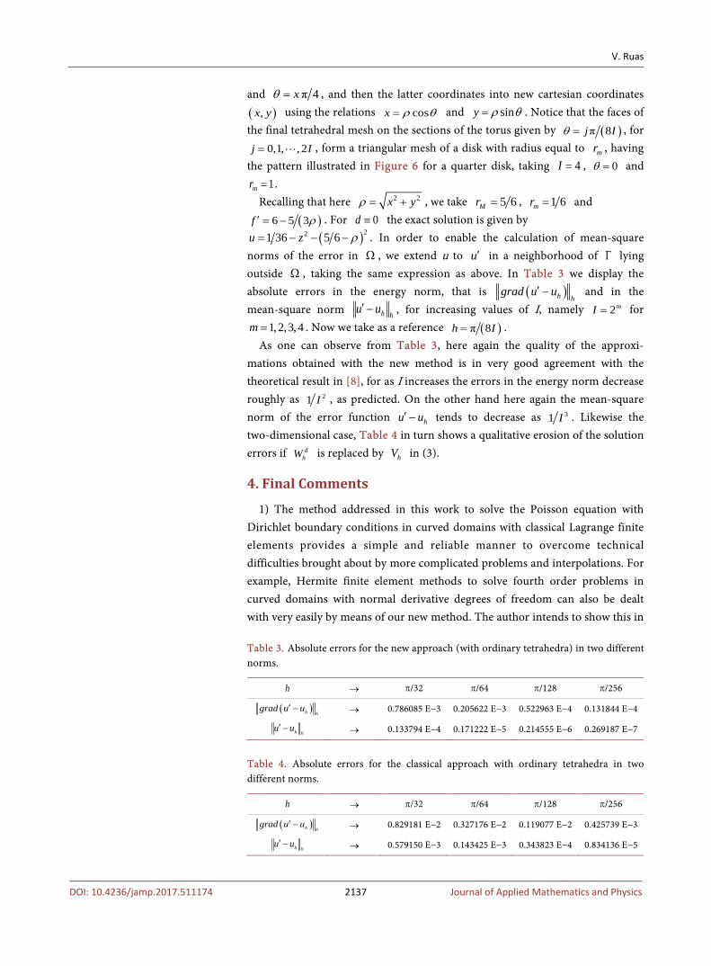
Recalling that here 2 2x yρ = + , we take 5 6Mr = , 1 6mr = and ( )6 5 3f ρ′ = − . For 0d ≡ the exact solution is given by

( )221 36 5 6u z ρ= − − − . In order to enable the calculation of mean-square norms of the error in Ω , we extend u to u′ in a neighborhood of Γ lying outside Ω , taking the same expression as above. In Table 3 we display the absolute errors in the energy norm, that is ( )h h

grad u u′ − and in the mean-square norm h hu u′ − , for increasing values of I, namely 2mI = for

1,2,3,4m = . Now we take as a reference ( )π 8h I= . As one can observe from Table 3, here again the quality of the approxi-

mations obtained with the new method is in very good agreement with the theoretical result in [8], for as I increases the errors in the energy norm decrease roughly as 21 I , as predicted. On the other hand here again the mean-square norm of the error function hu u′ − tends to decrease as 31 I . Likewise the two-dimensional case, Table 4 in turn shows a qualitative erosion of the solution errors if d

hW is replaced by hV in (3).

4. Final Comments

1) The method addressed in this work to solve the Poisson equation with Dirichlet boundary conditions in curved domains with classical Lagrange finite elements provides a simple and reliable manner to overcome technical difficulties brought about by more complicated problems and interpolations. For example, Hermite finite element methods to solve fourth order problems in curved domains with normal derivative degrees of freedom can also be dealt with very easily by means of our new method. The author intends to show this in Table 3. Absolute errors for the new approach (with ordinary tetrahedra) in two different norms.

h → π/32 π/64 π/128 π/256

( )h hgrad u u′ − → 0.786085 E−3 0.205622 E−3 0.522963 E−4 0.131844 E−4

h hu u′ − → 0.133794 E−4 0.171222 E−5 0.214555 E−6 0.269187 E−7

Table 4. Absolute errors for the classical approach with ordinary tetrahedra in two different norms.

h → π/32 π/64 π/128 π/256

( )h hgrad u u′ − → 0.829181 E−2 0.327176 E−2 0.119077 E−2 0.425739 E−3

h hu u′ − → 0.579150 E−3 0.143425 E−3 0.343823 E−4 0.834136 E−5


V. Ruas


a paper to appear shortly. 2) The technique studied in this paper is also particularly handy, to treat

problems posed in curved domains in terms of vector fields, such as the linear elasticity system and Maxwell’s equations of electromagnetism. The same remark applies to multi-field systems such as the Navier-Stokes equations, and more generally mixed formulations of several types with curved boundaries, to be approximated by the finite element method.

3) As for the Poisson equation with homogeneous Neumann boundary conditions 0u n∂ ∂ = on Γ (provided f satisfies the underlying scalar condition) our method coincides with the standard Lagrange finite element method. Notice that if inhomogeneous Neumann boundary conditions are prescribed, optimality can only be recovered if the linear form hF is modified, in such a way that boundary integrals for elements hT ∈ are shifted to the curved boundary portion sufficiently close to Γ of an extension or reduction of T. But this is an issue that has nothing to do with our method, which is basically aimed at resolving those related to the prescription of degrees of freedom in the case of Dirichlet boundary conditions.

4) Finally we note that our method leads to linear systems of equations with a non symmetric matrix, even when the original problem is symmetric. Moreover in order to compute the element matrix and right side vector for an element T in h or in h , the inverse of an k kn n× matrix has to be computed, where kn is the dimension of ( )kP T . However this extra effort is not really a problem nowadays, in view of the significant progress already accomplished in Computational Linear Algebra.

Acknowledgements

The author is thankful for the support provided by CNPq-Brazil, through grant 307996/2008-5, to carry out this work, which was first presented in August 2017 at both the MFET Conference in Bad Honnef, Germany, and the French Congress of Mechanics in Lille.

Sincere thanks are due to the managing editor Hellen XU for her precious assistance.

References [1] Brenner, S.C. and Scott, L.R. (2008) The Mathematical Theory of Finite Element

Methods. Texts in Applied Mathematics, Vol. 15, Springer, Berlin. https://doi.org/10.1007/978-0-387-75934-0

[2] Nitsche, J.A. (1972) On Dirichlet Problems Using Subspaces with Nearly Zero Boundary Conditions. In: Aziz, A.K., Ed., The Mathematical Foundations of the Fi-nite Element Method with Applications to Partial Differential Equations, Academic Press, Cambridge, Massachusetts.

[3] Scott, L.R. (1973) Finite Element Techniques for Curved Boundaries. PhD Thesis, MIT, Cambridge, Massachusetts,.

[4] Ciarlet, P.G. (1978) The Finite Element Method for Elliptic Problems. North Hol-


https://doi.org/10.1007/978-0-387-75934-0

V. Ruas


land, Amsterdam.

[5] Ruas, V. (2017) Optimal Simplex Finite-Element Approximations of Arbitrary Or-der in Curved Domains Circumventing the Isoparametric Technique. arXiv Nu-merical Analysis. https://arxiv.org/abs/1701.00663

[6] Ruas, V. (2017) A Simple Alternative for Accurate Finite-Element Modeling in Curved Domains. Congrès Français de Mécanique, Lille, France. https://cfm2017.sciencesconf.org/133073/document

[7] Nitsche, J.A. (1979) L∞-Convergence of Finite Element Galerkin Approximations for Parabolic Problems. ESAIM: Mathematical Modelling and Numerical Analysis, 13, 31-54.

[8] Ruas, V. (2017) Methods of Arbitrary Optimal Order with Tetrahedral Fi-nite-Element Meshes Forming Polyhedral Approximations of Curved Domains. ar-Xiv Numerical Analysis. https://arxiv.org/abs/1706.08004


https://arxiv.org/abs/1701.00663

https://cfm2017.sciencesconf.org/133073/document

https://arxiv.org/abs/1706.08004

variational formulations yielding high-order finite...

Documents