vehicle following control design for automated …ioannou/2003update/d50.pdfvehicle following...

Vehicle Following Control Design for Automated Highway Systems

H. Raza and P. Ioannou

A, utomatic vehicle following is an important feature of a fully rpartially automated highway system (AHS). The on-board

vehicle control system should be able to accept and process inputs from the driver, the infrastructure, and other vehicles, perform diagnostics. and provide the appropriate commands to actuators so that the resulting motion of the vehicle is safe and compatible with the AHS objectives. The purpose of this article is to design and test a vehicle control system in order to achieve full vehicle automation in the longitudinal direction for several modes of operation, where the infrastructure manages the vehicle following. These modes include autonomous vehicles, cooperative vehicle following, and platooning. The vehicle control system consists of a supervisory controller that processes the inputs from the driver, the infrastructure, other vehicles, and the on- board sensors and sends the appropriate commands to the brake and throttle controllers. In addition. the controller makes deci- sions about normal. emergency, and transition operations. Simu- lation results of some of the basic vehicle following maneuvers are used to verify the claimed performance of the designed controllers. Experiments on Interstate-15 that demonstrate the performance of the throttle controller with and without vehicle- to-vehicle communications in an actual highway environment are also included.

Introduction One of the objectives of Automated Highway Systems (AHS)

is to meet the increasing demand for capacity by the efficient utilization of the existing infrastructure. Capacity is calculated by the simple formula:

\7 C=- x, + L (1)

where Cis the capacity, measured in number of vehicles crossing a fixed p o i n t h i t time, Vis the vehicular speed of flow. X , is the inter-vehicle spacing, and L is the vehicle length. The capacity formula (1) is derived by assuming that all vehicles have the same length L, keep the same inter-vehicle spacing X,, and follow the same speed V. The capacity C can be viewed as the maximum possible flow rate q for a given speed V, inter-vehicle spacing X,, and vehicle length L. While the traffic flow rate may exceed C during transients by violating the maximum allowable V or minimum allowable X,, in an AHS environment such violations

The authors are nitfz the Departnzent ofElectrica1 Engineering-Sys- terns, University of Southern Cnlifornin, Los Angeles. This work is supported by the California Department of Transportation through PATH of the Univerrit), of California.

have to be reduced or eliminated for safety considerations. Therefore in AHS q has to be kept less than or equal to C during transients and C should be the desired value q should converge to in steady state. These constraints give rise to the following requirements:

(i) The system should be designed for maximum capacity under the constraints of safety.

(ii) The system should be designed so that the actual traffic flow rates tend to the maximum capacity at steady state and transients are not excessive and are not due to the violation of safety constraints on the vehicle level.

The first requirement can be met by using the safety considerations to decide about the maximum allowable speed V and minimum inter-vehicle spacing X, [l]. The second requirement can be met by designing the vehicle following control system properly, getting the infrastructure involved in managing traffic flow on the macroscopic level, minimizing disturbances due to lane changing, and choosing the appropriate configurations for the roadway system [2 , 3, 51.

The purpose of this article is to concentrate on the design of the vehicle longitudinal control system (VLCS) that will guarantee smooth and safe vehicle following. In an AHS environment the VLCS should be able to accept and process inputs from the driver, infrastructure, other vehicles in the vicinity as well as from its own sensors. The VLCS is designed for intelligent cruise control ( I C 0 applications, cooperative driving. and platooning. Using ICC, the vehicle is autonomous in the sense that it does not communicate with the infrastructure and/or other vehicles. In cooperative driving the VLCS may accept inputs from the vehicles in front and the infrastructure, w-hereas in platooning the VLCS has to process inputs from the leader of the platoon as well as from the infrastructure and other vehicles. These three different modes of operation may be necessary in AHS, and the design of a VLCS to operate in each chosen mode is therefore essential.

The VLCS consists of a supervisoy controller. which is the “brain” of the system, and a throttlebrake controller. Since several throttlebrake controllers have already been proposed and tested [6-111. the emphasis of this article is on the supervisoq controller and its interaction with the various inputs and the throttlebrake controller^ The design of the supervisory controller is similar to the design concept of event-driven state machine control. The design objective is to replace the human driver functions in the longitudinal direction. The throttle and brake controllers are used both in normal as well as in emergency situation to give complete automation in the longitudinal direction.

The emergency situation handling logic. as a part of the supervisory controller. is designed on the principles used by the human drivers to handle emergencies. It comprises a situation assessment logic to detect the presence of emergencies and a

December 1996 0272-1708/96/$05.0001996IEEE 43

compensation logic to handle emergencies of different severities. The effectiveness of this scheme relies on the quality of the sensors and actuators that can provide low detection and actua- tion delays. In addition, the supervisory controller chooses the mode of operation and handles the transitions from manual to automatic and vice-versa.

The article is organized as follows: Some of the possible AHS configurations are discussed next. The concept of vehicle longitudinal control and a detailed description of the design of supervisory controller are presented in the third section. The stability and performance analysis of the overall closed-loop system is given next, and following this the simulation and experimental results for different vehicle following scenarios are discussed. The article ends with the main results summarized in the conclusion section.

Basic Notation AVF: automatic vehicle following ICC: intelligent cruise control VLCS: vehicle longitudinal control system u : acceleration of the vehicle (m/sec2) 11: time headway (sec) W speed of the vehicle (mlsec)

hsub: variables associated with headway Vsub: variables associated with speed

boolean variables; szrb identifies each variable

AH§ Configuration and Modes of Operation A general AHS confignration that captures a wide class of

AHS concepts is shown in Fig. 1, where the infrastructure may issue speed and headway commands to the vehicles in an effort to produce uniform and homogeneous traffic flow conditions, which in turn can guarantee stable and higher traffic flows [12]. In this configuration a distributed control is exercised. where the control loop contains part of the infrastructure as well as the vehicle itself. In terms of the classification defined in [ 131, the

complete control hierarchical structure is shown in Fig. 2. The structure is defined in terms of different layers; the network and link layer lies with the infrastructure. whereas the coordination, regulation. and physical layers reside in the vehicle.

In terms of the structure shown in Fig. 2. the infrastructure control consists of the network and link layer or roadway controller. The network controller optimizes the operation of the traffic network by issuing routing instructions and traffic syn- chronization commands and by providing desired traffic distributions for the various branches of the network to the link layer or roadway controllers. The roadway controller manages a branch of the network snch as a large section of the highway. It receives desired traffic density distributions from the network controller and traffic flow measurements from the section and issues speed and headway commands to the vehicles in its section in order to change the traffic density to the desired one. The speed and headway commands can be transmitted by using the road side beacons (see Fig. 1) or other communication techniques.

The vehicles operating in the AHS configuration of Fig. 1 are equipped with the appropriate control systems that allow them to respond to the roadway commands as well as to the commands of the driver (during transitions). In addition, the on-board control systems have to be able to process the information received from their own sensors and. depending on the mode of operation, communicate and coordinate maneuvers with other vehicles.

The on-board control system includes the coordination and regulation layers shown in Fig. 2. The coordination layer consists of a supen7isory controller that is responsible for self-&agnostics, recognizing the desired mode of operation, communicating with the link layer, other vehicles, and the driver, and issuing appropriate commands to the regulation layer. The regulation layer consists of the throttle, brake, and steering controllers that are activated by the supervisory controller and generate the appropriate commands to the actuaton that reside in the physical layer.

In this article we concentrate on the coordination layer by designing the structure of the super\Visory controller for longitu-

A Section of Freeway

; -1 ; -1 1 - 1 1-1 1 - 1 -1

1 1 1 1 1 1 : I 1- I I_ I I ; Il I Il I

1 1 i ; 1 1 i ; I ; ; 1 1 I j : ; 1 1

1 1 1 1

1 1 1 1 I I I I I’ I I I I b7 I

Traffic Flow Measurements Trafflc Flow Measurements

f i Speed f i Speed \ V Y

Headway Roadway Controller

Roadside Beacon Roadside Beacon

Headway

Fig. 1. An 4HS conjprarion

44 IEEE Conhol Systems

r - I

Infrastructure Control

I i

1 Network 1 Network Controller

I Link I Roadway Controller

I Coordination Supervisory Controller

I Physical 1 Throttle, Brake, Steering Subsvstems

I I L

Fig. 2. Distributed control Jtructure for in$-astl-ucture ntanaged vehicle control.

dinal control that may be used for several modes of vehicle following operations described in the following subsections.

Intelligent Cruise Control (ICC) Intelligent cruise control (ICC) is a near-term device that will

allow automatic vehicle following under the possible supervision of the driver. In this case the driver sets the desired speed and headway and passes the task of vehicle following to the ICC system. The driver is responsible for steering and for recognizing and responding to emergencies. The roadway in this case may issue desired speeds to the driver using road signs etc.

The supervisory controller accepts and responds to the driver inputs: it monitors its on-board sensors, performs diagnostics, and sends the appropriate commands to the throttle and brake controllers.

Cooperative Driving (No v-v Communication) In this mode of operation, the roadway-to-vehicle communi-

cation capability is added to the ICC system. The roadway controller can now send speed commands to the supervisory

controller directly in order to control the traffic density along the highway lanes. The driver’s role and responsibility remain the same as in the ICC mode, except that heishe is not allowed to set the desired speed.

With this mode of operation the supervisory controller should be able to communicate and respond to the roadway commands in addition to respondiug to the inputs associated with the ICC mode.

Cooperative Driving (With v-v Communication) The addition of vehicle-to-vehicle (v-v) communication ca-

pability allows the vehicles to communicate with the neighbor- ing vehicles in order to negotiate and coordinate maneuvers and inform vehicles about braking capabilities, acceleration, deceleration, maneuvers etc. This extra capability can be fully ex- ploited if the ICC system is upgraded to detect and handle emergencies in the longitudinal direction. Since the control system becomes responsible for emergencies. the headway is no longer selected by the driverbut is chosen by the on-board control system.

For this mode of operation the supervisory controller should be able to handle and interpret the communications with other vehicles and detect and handle emergencies in the longitudinal direction in addition to the tasks associated with cooperative driving without v-v communications. One of the important tasks of the supervisory controller is to process all the available inputs and information and select the appropriate headway in order to guarantee collision-free vehicle following. In addition, the task of transition from automatic to manual is handled in a way that does not put the driver in a situation heishe cannot safely handle.

Platooning When the vehicles are capable of communicating with each

other and the roadway in addition to being able to follow each other in the longitudinal direction, it may make sense to organize them in a way that improves capacity without affecting safety. It has been proposed in [13] that the organization of vehicles in platoons of 10 to 20 with small intra-platoon but larger inter-platoon spacing (see Fig. 3) will increase capacity considerably. The organization of vehicles in platoons allows the roadway to treat

Roadway Controller

Platoon I

Fig. 3. Platooning of vehicles ns one possible mode of operation of AHS.

December 1996 45

I - - - - - - - - -

Fig. 4. Vehicle longitudinal control system.

each platoon as a single entity and therefore eases the requirements on the bandwidth of the roadway-to-vehicle communication system. Therefore, instead of communicating with each vehicle independently, it communicates with the leader of each platoon. The platoon leader in turn communicates with its vehicles in order to make sure the whole platoon operates as required according to the roadway commands and the traffic conditions. Since each vehicle could become a leader the supervisory controller should be designed to handle the case where the vehicle is a follower and a member of platoon as well as the case where the vehicle is a platoon leader.

The reasons for considering different modes of operation are the following:

1. The vehicle should be able to operate on non-AHS facilities. Since the ICC system is developed independent of AHS. the XHS vehicle should be able to operate as any other vehicle equipped with ICC on non-AHS facilities.

2. During certain failures or traffic conditions platooning may not be the most appropriate mode of operation. and the system may have to operate in the cooperative driving or even ICC mode.

Vehicle Longitudinal Control Design The block diagram of the Vehicle Longitudinal Control Sys-

tem (1’LCS) is shown in Fig. 4. The supervisory controller accepts inputs from the roadway, driver, other vehicles, and its on-board sensors. It processes these inputs and performs some or all of the following tasks:

1. Determines the current mode of operation, Le., ICC, cooperative drhing, platooning etc.

2. Performs the transition operation, from manual to automatic and back to manual.

3. Selects the desired headway and speed for normal operating conditions.

4. Detects and handles emergency situations in cooperative driving and platooning.

The design objective of the supervisory controller is to smoothly execute these tasks without risking the safety and comfort of the occupants. The details of these tasks are given in the following subsections. A detailed block diagram of the proposed supervisory controller is shown in Fig. 5 .

46

Selection of AHS Mode The different modes of operation of AHS are classified in

terms of distribution of authority between the driver and external agents, such as infrastructure, platoon leader. and surrounding vehicles. Since the vehicle will be using some means to communicate with the roadway and other vehicles, it is safe to assume that these signals will be tagged or labeled to identify the source of information. Hence the logical wa~7 for determining the mode of operation of AHS is to detect the presence or absence of certain input signals.

In case no speed and headway commands are received from the roadway or platoon leader and no communication is estab- lished from the leading vehicle. ICC mode is selected. In case speed commands are received from the roadway only and no communication is detected from the platoon leaderileading vehicle, cooperative mode with no v-v communication is selected. Similarly. other operating modes are selected based on the presence of necessary commands from the external agents discussed in the previous section.

Transitions The driver initiates the transition by giving the “automatic

vehicle following (‘4VF) on!’ or “AVF off’ input to the driver interface module of the supervisory controller. The driver interface module assigns a value to the signal 5D0n (.) to be used by the transition logic as shown by the flowchart in Fig. 6.

The transition module uses two logical signals, 5D0m (.) ~ &(.)

and on-board sensor readings to decide if the requested transition operation is safe to execute. For transition from manual to automatic, the driver selects the “’AW on” command that assigns a value of 1 to the signal sDor, i.) . The transition module then checks the working status of all subsystems and assigns the value Bs = 1 if the system is free of faults, otherwise B, = 0 is assigned. The checking of operating status of the system is a continuous process of self-diagnostics using sensor measurements and fault- detection algorithms; hence the automatic mode is transitioned to manual at any time a serious fault is detected.

At the end of trip, the driver initiates the automatic to manual transition process by giving “AVF off’ command. This switching

IEEE Control Systems

process involves the steps that are taken to make the driving conditions suitable for human capabilities. This is achieved by slowing down the vehicle and increasing the headway, so that the driver can easily drive the vehicle off the auto lane. The output and (l?(k) 2 h,, and V ( k ) 5 I/,,, ), (2) of transition logic, BAon , w-hich shows the status of AVF, is a

logical signal having values { 1 ,O] and is given as: where V. h are the vehicle speed and headway respectively, V,,,,

1 1 if ( k ) = 1 and B y ( k ) = 1

B~,,, ( k ) = 0 if ( B~~~ ( k ) = 0 or ~ , ( k ) = 0)

AudioiVisual Information/Warning I I I

I I _ _ _ _ _ _ _ _ _ - - - _ - - - _ _ I I

I I I

I I ThrottlelBrake i Throtjei I I I Switching

A I I Brake OniOff

Transillon I I I

Logic I I I

I

I b I

Human Driver I Transitions

I I I I I I

I ] Desired I fi Speed

- I I

I I I I I I I I

SpeedlHeadway I I ; - I

AHS Mode Selection

I I I I I

I ’ Desired

Headway I -

_T.a_nSi!!iO_”_s ?Eo!: - _ _ I - Selection

I I

I I I I I Emergency

I Situation I I

I _ _ _ _ _ _ _ _ _ _ _ _ - _ _ _ _ I I Interface

Assessment

Fig. 5. Detuilecl structure ofthe supewisoly controllel:

r

Set Default Speed & Headway

L

Fig. 6. Logic f o r transitions.

December 1996 47

and h,, are the design constants, and k represents the sampling instant. As gilen in 12), the current speed and headway are checked against certain thresholds. and speed and headway are progressively increased by speed a:~d headway selection logic till they reach the required limits. It should be noted that the process of transition from manual to automatic is the same for all modes of XHS; however. the transition back to manual mode may be different for each mode. For example, the thresholds

h,,, m-ill be different for ICC than the cooperative driving and platooning. The requirement of making the driving conditions suitable for human drivers is more strict in modes of AHS where the driver is not responsible for emergency handling, such as cooperative driving with v-v communication and platooning.

Automatic Vehicle Operation After AVF is switched on, Le.: when the transition logic has

the output BAoo = 1 , the supervisory controller proceeds with the

selection of the mode of automatic vehicle operation. Two different modes of automatic vehicle operation are possible and are determined hq the presence or the absence of a valid target. If there is a vehicle or obstacle, referred to as target, within the designated sensing range then the supervisory controller will choose the follow mode and if there is no target the controller will choose the cruise mode as shown in Fig. 7. The conditions for a valid target are the following: (i) The target is within a designated range that is chosen a priori based on safety considerations. (iij The speed of the target is less than the speed selected by the driver (in ICC modej or the roadway/platoon leader commanded speed (in cooperative drivingiplatooning mode).

If either of these two conditions is violated, the vehicle in front is not considered to be a valid target to follow. The conditions given above can be combined to form a "follow target" condition BF(.) as:

AVF On

I !%m='

A i v "Follow" w "Cruise"

hd "d L

Fig. 7. Operating mode selection logic.

[l if BAGM ( k ) = 1 and [

i s , ( k ) = ' { h ( k ) < h, and ( K ( k ) < V, (k )+ A,)}or I ((V'(k) < V,(k) + A2) and B F ( k - 1) = 1}]0 (3)

where ht is the threshold for headway calculated from the sensing range, Vl is the speed of the leading vehicle, Vc is the roadway- or driver-commanded speed, and AI , A2 > 0 are design constants. In (33 A2 > A1 is used to avoid the unnecessary switching of the targets caused by the transients andor sensor noise; hence if the target was preyiously being followed then a larger fluctuation in target speed is tolerated. The design constants AI, A2 may be different for different modes of AHS; similarly the commanded speed Vc is different for each mode, e.g., Vc is the speed commanded by the driver in ICC mode, and so on.

As shown in Fig. 7, if the vehicle is in follow mode the supervisory controller has to select a safe headway. The calculation of the safe headway is done by the headway selection logic, which uses the inputs from the &her, roaciwa>-; and other vehicles for different modes of AHS. In the follow mode the desired speed is the speed of the leading vehicle. Similarly if the vehicle is cruising, the safe cruising speed is calculated by the speed selection logic. The process of safe headway and speed selection is explained in the following subsections.

Desired Headway §election After AVF is switched on and the vehicle is operating in the

follow mode. the desired headway selection logic has to initialize the system with a safe headway. This initializing value is taken to be the same as the actual headway h(.), irrespective of the mode of operation of AHS. After this initialization sequence, the headway selection logic allows the driver or the external agents to change the desired headway as long as this change does not risk the safety of the system. A logical structure of this selection process in shown in Fig. 8. The switching logic shown in Fig. 8 contains all of the decision making process for the desired headway calculation. It generates the desired headway hi as a nonlinear function of its inputs. A filter D ( z ) is used to generate the filtered version of the desired headway hd. T i e details of different tasks performed by the headway selection module are given below. These tasks are different for each mode of operation of ,4HS and will be defined separately

Fig. 8. Block diagram of the desired 1zeadwa:g calculation

48 IEEE C o n t d Systems

i’ Headway Increase

Bh+= 1

Switching Logic

off 5hk’ ’ [ )

Headway Decrease

Fig. 9. State diagram f o r headway switchiizg logic.

ICC and Cooperative Driving Without v-v Communica- tion. The state diagram of switching logic for this case is shown in Fig. 9. A “headway reset“ operation is performed during initialization or whenever the “follow” mode is switched on. During this the value of hd(.) is chosen to be the current headway h(.) as long as it is greater than the minimum allowable headway h,,,. This task is performed irrespective of the mode of operation of AHS and ensures that there are no large transients, even though the conditions at switching are not close to the desired ones. Hence the value of hd(.) during reset operation is:

where BRA (.) is the condition used to trigger the headway reset

operation. As pointed out before that a resetting operation is performed by the switching logic whenever the AVF is switched on or a valid target appears in the cruise mode. The reset headway command BR;, (.) is calculated as:

I 1 if (BAoq ( k ) = 1 and Bh0,. ( k - 1) # 1)

or (B,(k) = 1 and BF(k - 1) # 1) 0 else. ( 5 )

Since in ICC and cooperative driving without v-v communication, the driver is allowed to adjust the headway according to hisher comfort leliel, the requests for headway changes are processed by using the “headway increase” and “headway decrease” operations shown in Fig. 9. The headway is increasedide- creased by a predefined step size Ah and this change is accomplished through the output signal hi(.) from the switching logic given below:

Ah if ’B,, ( k ) = 1

0 else, (6)

where B, (.) , ah_ (.) are the conditions for starting the headway increase and headway decrease operations, respectively. The headway decrease operation is triggered only after detecting a headway decrease command from the driver. On the other hand, headway increase operation can also be started by “transition to manual’’ operation. As shown in Fig. 6, a transition to manual operation is performed whenever the driver wants to switch off the AVF or a fault is detected in any critical subsystem. However, as given in (2 ) , the transition operation requires that the headway be greater than certain threshold h,,, and the speed less than V,,,. All of these conditions are formulated in the form of logical signals Bb+ (.) and Bt- (.) given below:

%+ ( k l = { I

I if (B , (k ) = 1 and B , ( k ) = 0) or B40f ( k ) = I 0 else (7)

% ( k ) = 1 if B,(k) = 1 and B,(kj = 1 and BA9,,(k) = 0 0 else , (8)

where BH(.), (.) are the conditions for processing the headway commands from the driver and transition to manual operation, respectively. The condition used by the switching logic to process the headway commands from the driver. !%Sa), ensures that 11 E [lamin. h m a X ] and is given below

BH ( k ) = 0 if BDh (kj = 0 and h ( k ) < h,, and lzd ( k - 1) < h f z T

1 if BDh ( k ) = 1 and h(kj > h,, and h, ( k - 1) > h , , l(9)

where h:d>. is a design constant and BDh (.) is an output signal from the driver interface to process the headway changes requested by the driver, BDh = 0 when the driver wants to increase the headway and BDk = 1 otherwise. As pointed out before, the qignal BAof (.)

tests the conditions at the time of transition to manual mode and is given as:

1 1 if (B,4<,n ( k ) = 1 and (BDnn ( k ) = 0 or B,(kj = 0)

BXo.l ( k ) = and ( h ( k ) < h,, or V ( k ) > V m a y ) and h,(k - 1) htah]

(10)

As shown in Fig. 8, the headway command generated by the switching logic hi(.) is filtered to avoid excessive transients. The filtered desired headway command hd is given as:

0 else.

h d ( k ) = h d ( k - 1) + Th,(k). (1 1)

where Tis the sampling time and hi(.) is given in (6). Cooperative Driving with v-v Communication and Pla-

tooning: The state diagram of switching logic for this case is shown in Fig. 10. Ar pointed out before. the “headway reset” task is same for each mode of operation of AHS, hence the relations in this case are the same as given in (4) and (5) . However, the design constant hnzin may be different for each mode of AHS.

In ICC and cooperative driving mode without v-v communication, the actual headway h is taken as the desired headway

December 1996 49

5F= 1 and 5An,,= 1 w

L

Fig. 10. State diagvanzfor headway switching logic.

command from the driver, with the assumption that the driver will switch on the AVF when the vehicle is following the preced- ing vehicle at a comfortable distance. However. in cooperative driving uith \--x- communication and platooning modes the headway h at the time of resetting can be different than the roadn-ay commanded headway IZR, (in the case of platooning h~ is received indirectly through the platoon leader). The desired headway in this case is smoothly changed to h R by using the “headway track’ operation shown in Fig. 10. Also shown in Fig. 10 is the “head- waq- increase” task, which is performed only when the transition to manual mode is required. The output of the switching logic hi(.) in this case is:

where kp is a design constant 9,40k (.) and is the same as siven in

(10). In (12) it is assumed that h~ E [hmin,lzmax]. Again the filter D(z) given in (11) is used in this case too. For reference a complete expression for the desired headway command hd(.) is given below:

h , ( k - l ) + T h ( k ) else. (13)

where hi(.) is given by either (6) or (12) depending on the mode of operation of AHS.

Desired Speed Sdection If the vehicle is operating in the cruise mode, the speed

selection logic calculates a desired speed to be given to the throttlebrake controller. If the vehicle is operating in ICC the desired speed is selected by the driver while in cruise mode. In this case the vehicle is tra\,eling without any valid target in front. In the case of cooperative driving and platooning, desired speed is issued by the roadway. While platooning the vehicle can be in

I 5R* = 0

~

Fig. 1 I. State diagram for the speed switching logic.

the cruise mode only if it is a platoon leader. The structure of the desired speed selection logic is the same as that of the desired headway, shown in Fig. 8. The functions performed by the switching logic in this case are given below.

The state diagram for speed sw-itching logic is shown in Fig. 11. For the desired speed selection we are assuming a different kmd of driver interface in which the speed command from the driver is available in exact numbers instead of increase/decrease command considered for headway selection. Hence the state diagram shown in Fig. 11 is the same for each mode of AHS; the only difference is that the speed command for “speed track” operation has different sources.

A “speed reset’‘ operation is performed whenever the AVF is switched on and the desired speed is taken as the current speed of the vehicle V. This resetting condition avoids large speed transients at the time when the AVF is switched on. Hence

y ( k ) = V ( k ) if B R 3 ( k j = l , (14)

where BRs (.) is the speed reset command and is generated as:

After initialization, the desired speed vd is made to track the speed command VC through “speed track” operation. The speed switching logic generates a signal V i ( . ) which is passed through a filter D l ( z ) designed with comfort constraints. The speed command Vi generated by the switching logic is given as:

where k, is a design constant, Satl(.), Sat2(.) a e saturation functions and B4m (.) is the same as given in (10). which is used

to determine whether the speed and headway at the time of transition to manual mode are wTithin the specified limits. In (16). r(.) is given as:

where Vs > 0 is a design constant and is the vehicle speed when the control is finally transfered to the driver after transition, usually taken to be equal to the nominal highway speed. The signal s(.) in ( 1 7) chooses the source of desired speed cammand for different modes of AHS and is given as:

IEEE Cotztl-ol Systems

Emergency Situation Assessment: The presence of a poten- tial emergency situation is estimated by detecting an unusual

(18) pattern in the input signals. The common kind of emergencies

where Vi is the speed of the leading vehicle and Vc is the speed command provided by the driver or infrastructure. As discussed before, in ICC mode Vc is issued by the driver. whereas in cooperative driving and platooning Vc = VR. However, in platooning mode. only the platoon leader can operate in the cruise mode and hence can receive speed commands from the roadway. The rest of the platoon takes the desired speed and headway commands through the platoon leader. It will be shown later in the simulation section that the conditions for following a target given in (3) and switching the desired speed from the leader speed to the roadway speed as given in (18), prevents excessive overshoot when the platoon executes a slowing-down maneuver. The speed command Vi(.) is passed through a filter Dl(z ) which is given as:

T/d(k) = Vd(k - 1) f mi(k) . (19)

It should be noted that (r(k - 1) - V& - 1)) in (16) at the input of the integrator (19) is an acceleration term. Therefore the comfort constraints imposed in terms of maximum allowable acceleration and deceleration are given in (16) as saturation functions, Sutl(.) and Sat2(.), where

A,, if ( r - V,) Z A,,, Aman if ( r - V,) < Aroi,z r - V, else (20)

encountered while driving in the automatic following mode are: 1. subsystem failure 2. potentially dangerous target in cruise/follow mode For detecting subsystem failure, the assessment logic receives

operating status of all the major subsystems of the vehicle. In case a failure is detected in any critical subsystem by the failure detection logic. an emergency situation is declared to be present.

The presence of a potentially dangerous target while operating in the cruise or follow mode can be determined by comparing the measured time to collision (TTC) against a minimum time for stopping the vehicle safely. At any time t, the relative distance X, between the vehicles can be written as:

where K and b a r e the speeds of leading and following vehicles respectively. a] and q are the accelerations of leading and following vehicle, respectively, and to is the time at which the measurement of TTC is required. If for some time t > to X,(t) = 0. then TTC = t - to. Since the calculation of TTC requires prediction of the deceleration profiles for the leading and following vehicle for the time interval [to, f], different assumptions can be made to approximate its value. For a rough cut estimate of TTC. we can assume that q ( s ) = al(s) V T E [to, t ] . Also with the assumption that the ranging sensor provides both the relative distance and speed information. the TTC can be calculated as:

P C = - Ax A v

[ r - V, else (21) where AX = X,(to) and AV = V&o) - Vi(to) are the measured relative distance and speed respectively at time to. For TTC to

where A,,, A’,,, > 0 and Amin, A’,ii1 < 0 are design constants. have any significance it is required that AV > 0. For a more The limits for maximum allowable acceleration and deceleration conservative estimate of TTC, we can assume that the leading are different during transition to manual mode, which is obvious vehicle is decelerating with the maximum possible deceleration from (20) and where A,,,, 5 A’,,, and A~~~~~ 2 A ’ ~ ~ , ~ , For allowed in emergency condition and the trailing vehicle is brak- reference, a complete expression for the desired speed command ing with maximum deceleration allowed in the automatic follow- Vd.) is given below: ing mode, i.e.. a l ( t ) = ai.! , U ~ T ) = a,,,in V T E [to, f ] , then:

where nrnirl is the maximum deceleration allowed in the automatic following mode and air,* is the maximum possible deceleration of the leading vehicle. From (25 ) , TTC can be written as: Emergency Operation

In cooperative driving and platooning modes, the recognition and handling of emergencies is one of the tasks performed by the supervisory controller. The recognition of emergencies requires TTC = -AV + d w that the input signals be continuously monitored for detecting 2Aa (26) the presence of any abnormal pattern or behavior. Once an emergency situation is detected, a set of actions is performed by where &I = %in - aln,,,, ’ ’ The Of TTC lies be- an emergency handling logic. The recognition and handling of tween that given in (24) and (26); however, from the safety point emergencies is discussed in subsections below. of view, we will use the more conservative estimate given in (26).

December 1996 51

(34)

where M is the mass of the vehicle and V and h are the current speed and headway of the vehicle, respectively. Hence the change in desired headway, Ahd, and the desired speed, AVd, can be calculated by scaling down their maximum values, Ah:,, and AY,, b , respectively. Le.,

Ahd = i 1 - e -"1 L 1 (35)

Hence, with the existence of an emergency, the calculation of the desired headway and speed can be changed as:

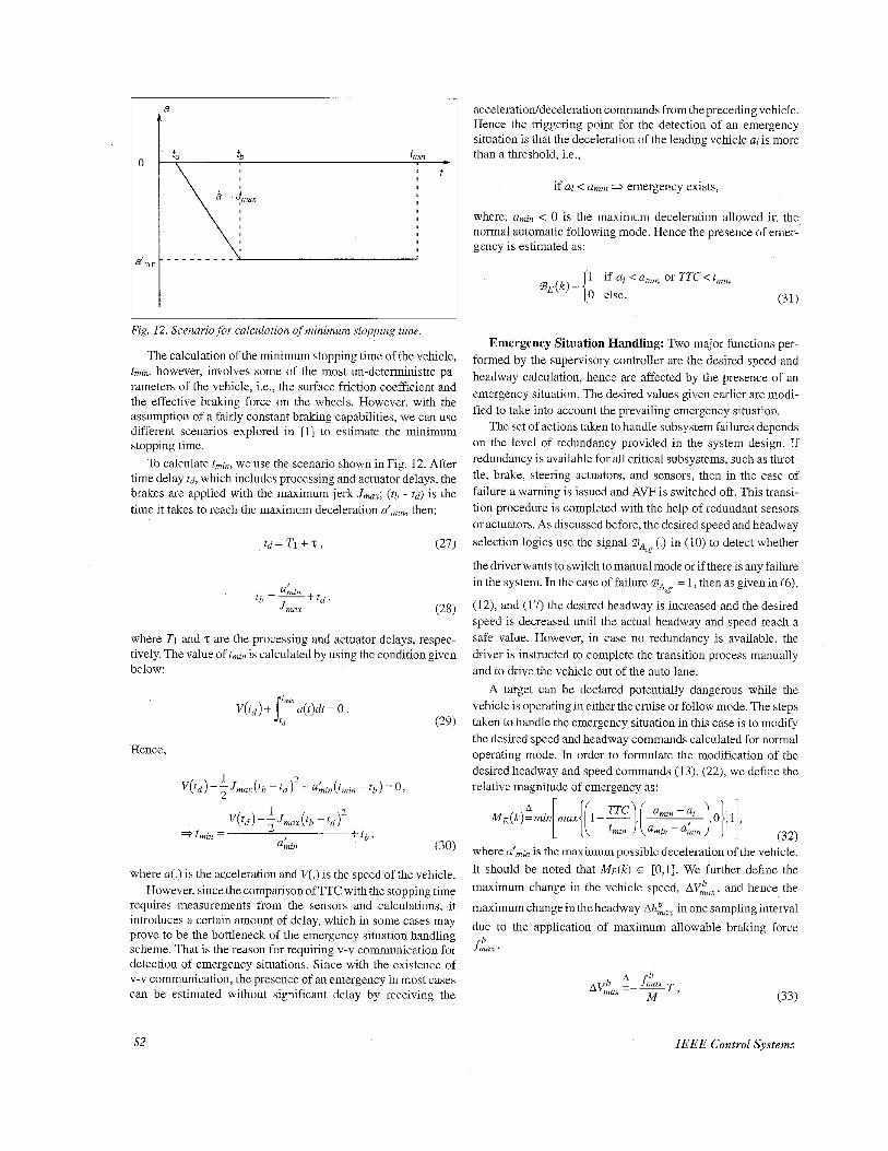
The simulation results for an emergency situation in which the leading vehicle slows down with a constant deceleration of 0.3g is shown in Fig. 13.

Stability and Performance Analysis In this section we will analyze the stability of the overall

closed-loop system shown in Fig. 4. For analysis purposes the block diagram is redrawn in Fig. 14. showing all the states and

5 10 15 20 25 30 S 0.5 5 - E

Time (Sec) L

Fig. 13. At to = 10 sec the lending lxehicle slows down nt n constant rate of -0.3g. The following vehicle with Xr(to) = 19.5 m (corresponding to time headway of 0.8 sec) manages to stop without collision.

December 1996

input/output for each block separately. For completeness' sake we will briefly describe the vehicle dynamics model here; a complete study can be found in [lo, 14, 151.

Two control inputs, the throttle angle and the braking torque, are used to control the motion of the vehicle in the longitudinal direction. The speed of the vehicle V is a nonlinear function of the throttle angle 8, i.e.,

v- m , t, 7) . Various expressions for the nonlinear function F(8. r: 2) exist

in the transportation literature and can be found in [14. 151. For normal vehicle operation, the nonlinear model (39) can be ap- proximated by a linearized model given below:

- n

V b -=- e s + 2 i ' (40)

where = V - V, and e = 8 - eo are the deviations of (V, e) from

the operating point (Vo, 80) and the model coefficients 2. are function of operating point. The model (40) can be rewritten as:

v=-L?vtietd, (41)

where the disturbance term, d, accounts for the neglected dynamics in (40). Similarly, the dynamic equation of the braking torque to the vehicle speed is given as:

"-(- I CLTb - fo - c 2 v - c3v'), M (42)

wh$re T b is the braking torque, M is the vehicle mass. fo. c2V. c3V- represent the static friction force, rolling friction force, and air resistant force respectively. The term CITb in (42) is the braking force and is proportional to the brake line pressure P,- shown in Fig. 14 as a control input. For this study we will use the nonlinear PID throttle controller and the brake controller designed with feedback linearization in [lo] to represent the throttlehrake controller in Fig. 14. Since the throttlehrake controller requires continuous signals as the desired speed and headway, the discrete time signals Vd(k) and hd(k) are filtered to generate continuous signals Vc(t) and hc(t), respectively. shown in Fig. 14. For throttle controller. the dynamic equations of the yehicle following are:

x ,=y-vf , Vf =-zipj - v , )+&,+d ,

6 = X r - h V f - S o .

v,=F-vf , (43)

Fig. 14. Closed loop system for stability analysis.

53

where 8 is the deviation from the desired spacing, VI is the speed Since the headway changes occur only at a finite number of of the leading \-ehicle (desired speed); V, is the relative speed, So instants, on requests issued by the driver or roadway, the signal is a constant. and e, = g, - eo is the throttle angle to be gener- hc(t) is mainly COnStant with finite number of transitions. W-ithOUt

ated by the control law. For PID controller Gf is given as: loss of generality, we can assume that one such transition occurs at to, then h,(tj can be represented as h,(r) = h(to) + hj(l -

determined by the filter Cz(s). Hence - ')), where hj is the jump in headway at time to and a is a constant 8~ = klV,. + k26 + (k3V, + k,6)dT. 6 (44)

- The gains kl , . . kd are chosen to place the closed-loop poles at h, ( t j = It, + hA , (46) the desired locations. In [lo] it is shown that the control law (44) guarantees that with constant h and V L 6: Vr + 0 (exponentiallJ9. where zc = izjto) + hj is constant and h, ~ -hje-u(t-b), Then for Similarly for the brake controller the closed-loop system after feedback linearization is: t 2 to the closed-loop system (433, (44) becomes:

where k5 and kg are the gaim to be selected to make the closed- loop system stable and to guarantee that 6. V,. + 0 for constant 11 and L'l, However, with the supervisory controller in the loop the desired speed and headway Yc1r) and /I&) cannot be assumed to be constant. Hence some analysis is required to show the closed loop stability with time varying desired speed and headway commands. In the analysis to follow, we will use the following Lemma [16].

Lemma 1 If the linear system:

i = A ( t ) x where 4 is con,tinuous b't 2 t o ,

is unifomlly asynzptotically stable (u.a.s.) fhen the system:

x- = [A( t ) + B(t )]x ,

is also u.n.s. $ i f f ) is continuous k' t 2 f0 and i f i i t ) -+ 0 as t +

Using Lemma 1, the following Theorem establishes the stability of the closed-loop system shown in Fig. 14.

Theorem 1 (i) All the signals in closed loop sJstem ofFig. 14 are bounded. (ii) i fV, jk) + C I and hdik) --f CZ, where C I , cz > 0 are constants then 6, Vr + 0. Proof: (i) The boundedness of the closed loop signals will be shown in two steps.

Step 1. As shown in Fig. 14, the supervisory controller with the filters generate the desired trajectory, hence in first step we will show that Vc(t) and hc(t) are bounded. The switching logic in the speed and headway selection logic guarantees that Vl(k) E

[VmtlJ,VJfia] and hi@) E [hnliil, hm,]. From (22) and (13) we have that lid&); h&) E 1,. Also, the filters Dl(z) and D(z) in (22) and (13) are designed so that AI7&), Ah&) E 1,. where Af(k) =S(k) - f ( k - 1). Since Vc(s) = Cl(s) Vd(k) and h,(s) = Cz(s)hd(k) with Vd(kj, h&) E L , filters Cl(s) and CZ(S) can be designed such that V,, T', E Ln mdh,, h c E L.

OQ.

Step 2. Before analyzing the stability of throttlehake system, w e consider the possible variations in the headway signal h&).

The terms So and d in (43) are constants and have no effect on the current analysis. hence are neglected in (47). The closed-loop system 147) can also be written as:

Y = [ C + D , ( t ) ] X + Du, (48)

where X = [X,., Vf] , u = [V,, tc] . Y = [F. b7,]'. The matri-

ces 4, B , C, D , Dl( t ) . and D2(r) in (48) are given as:

. T T

0 -1 0 1

ik4 -i(k2 + k, f k&) -(2 + ik1 + 6k2iZc)

1 0 1 B = [ 0 0 / ,

b(k,k,) -p + b k l ) i ~

c= [ 0 1 -It, -1 - 01; 0 D=[l 0 o;' 0-

Ir should be noted that (A& C,D) from (48) are the same as that for the closed-loop system (43), (44) with h = h, and Vl = V,. Now consider the homogeneous part of the LTV system (48):

54 IEEE Control Systems

60 . Test 1 : Case 2

. . . . . ,-xj . ' . '

5 5o F!: ..:. . . . . . . . . . . . . . . . . . . . . . . . . I . . . . . . . . . . : . . . . - d :

. - --_____

m o 20 40 60 80 100 120

8 ,!-,\ I . . . . . . I . . . . . . . . . . . . . //<: , 0.5

. . .

f 0 0

I \ E

20 40 60 80 100 120

E o 2 -10 h

20 40 60 80 100 120 9 0.2

g 0 e ' - I .

10 ~ - : '$ ' - - - - - - - - -

c

g-o ,2 20 40

/<It\ , \ : .- I '

60 80 100 120 Time (Sec)

Fig. 15. Follower sw'itches on AVF at t = 3 sec with r/f= 45 ntph and hf = h-R = 0.8 ser. AVF is su'itched off ar t = I00 see.

Since i = AX is an exponentially stable system. Dl(t) is continuous V t 2 to and Dl( t ) + 0 as t + -, then by Lemma 1 we have that (49) is u.a.s. Now (49) is u.a.s. if and only if 3 ?a. ao > 0 3 l~@(t ,~) l lS hoe-'"('-r) , for to 5 7 I t < w, where @(.,.) is the state transition matrix for (49). Since in step 1 we have proved

that u = [ V,, E L, , by solving the LTV system (48) for X and

Y, we have that:

where a1 = I1 B I/-, a2 = supi I1 C + Dz(t) Il, a3 = I1 D 11-. and E is a term exponentially decaying to zero due toX(t0) # 0. Hence X , Y E L. The same analysis can be shown for the brake controller (45). Since the throttlebrake switching logic designed in [lo] guarantees that the throttle and brake controller are not acting together at the same time. all the signals and states in the closed loop system in Fig. 14 are bounded. (ii) To show that 6, V, + 0 when Vd(k). hd(k) + constant. we will use another representation of the closed-loop system. From (43) and (44) we can get the transfer function from to 6 and V, as:

I 50 0 20 40 60 80 100 120

I 20 40 60 80 100 120

2 , l

-2'

$ 0'

3 -0.2

, 5 0.2

0 20 40 60 80 100 120

0 3 i-l :

, . - . i -

20 40 60 80 100 120

I Time (Sec)

Fig. 16. Follower switches on AVF at t = 20 sec with \(f = 55 nzph and h f = 0.6 see. AVF is switched o f a t t = I00 sec.

where A(s )=s3+( i+&q + ~ k z h ) s 2 + ~ ( k 2 + k 3 + k 4 h ) s + ~ k 4 .

With supervisory controller in the loop. (51) becomes:

;=[A, + ~ ~ ( t ) ] e + ~ ~ i { ,

Y = [cl + 04(r)]e , (52)

where e E $, ( A I , B I , CI) is a state space representation of (51) in the controller canonical form, D3(r) and D&) are exponentially decaying to zero disturbance matrices obtained by replac- ing h with h,(t) given in (46). Since &(t) follows the conditions s ta ted in Lemma 1. e=[A ,+D3(r ) ]e i s u .a . s . Now as

Vd(k) + c1 + V, + 0 . (52) is a u.a.s. system with a bounded input that goes to zero, hence Y = [6. V,IT -+ 0. The same result can be shown for the brake controller (45).

The simulation results in Figs. 17-1 8. where the desired speed and headway commands are made to change, support the claim asserted in Theorem 1.

Platoon Stability In this section we will establish the conditions the supervisory

and regulation layer controllers have to follow to guarantee the stability of platoon of vehicles. We will use the following definition for platoon stability.

Definition 1 A platoon of vehicles of length n is called stable 811 &,(ti I I - < II 61.r ( t ) 1 1 - and I ~ V ~ ( ~ ) I I ~ < ~ ~ ~ ~ - ~ ( t ) ~ ~ ~ , i = 2 ... Iz.

where 6 is the deviationfrom the desired spacing and V, is the relative speed between two vehicles.

Before we analyze the stability of platoon, we will make the following assumption. Assumption: A-I Speed fluctuations between any two successive vehicle in the platoon are within the limit A2 defined for the leading vehicle to be a valid target, Le., =

December 1996

._ 1 m I , . . . .

I

20 40 60 80 100 120 Time(Sec)

Fig. 17. At t = 60 sec, VR changes from 55 to 65 mph

By using Definition i and assumption A-I, the following theorem establishes the coadi~ions for platoon stability. Theorem 2. Under assumption A-I. a platoon of vehicles is stable if:

Where clo, . k2, and k3 are as defined in Theorem I . Proof: With supervisory controller in the loop we have 6, (s) = G5(s)V,, :using assumption4-I we have &is) = G&)L'i.1.

The transfer function relating 6i and &.I can be found as:

where Vks) = Wl(s)V,.~(s). Similarly. we can show that

- = W, (s) . Hence a sufficient condition for platoon stability

is that:

1; is)

(3)

From the closed-loop system (37) we have:

Since WlOj is the transfer function between Vi and V l - l , (55 ) can be written as:

bl =[I 0 b(k2 + k;)] ; c1 = [0 1 01 T

As proved in Theorem 1: il = [ A + Dl(r)]X, is u.a.s. and

I l ~ ~ ~ l 1 1 , 5 - ' hoc1

a0 ( 5 8 )

Since a1 = IlbllI_ = max{l, b(k2 + k j ) } , the sufficient condition for

platoon stability is:

It should be noted that the condition (59) puts a limit on the closed-loop poles of PID controller and the choice of filter C~(S).

Simulation and Experimental Results The automatic vehicle following (AVF) controller designed

in the third section i s sirnul&ed using the PID throttle/brake controller designed in [lo] and a nonlinear longitudinal vehicle model [lo]. The values chosen fol- different design constants in the supervisory controller are given below:

ht = 2 sec, A1 = 2.5 mph, 112 = 5 mph. (see (3)),


h,, = 1.2 sec, hnlin = 0.25 sec. h,i',,, = 1.5 sec, V,, = 65 mph.

kp = 0.1, A/, = 0.02, kl = 10. (see (12), (6), and (16)), At,,, = 0.7, Amin = -0.4, A',,, = 0.7, A'miit = -2. (see (20) and

V, = 55 mph. (see (17)). The design constants for the throttlebrake controller [ 101 and

the constraints for maximum acceleration, deceleration, and jerk are chosen as:

(see ( 9 ~ (10)).

(21)).

( l ) j j = 0.1, 5 = 1, ho = 1.2, k5 = I , kg = 0.25, nnlm = 0.2g, antirl = -O.2g,jIna = s m~sec3 . The logic switch designed for throttle and brake controller

[ lo] requires three parameters, Xmin, X,,,, and VI. The values chosen for these parameters are:

X,i, = 6 m. X,, = 40 m: V I = 13.4 mlsec , Three different tests are simulated to investigate the perform-

ance of the designed controller under different operating conditions; these are given in the subsections below. Finally, the test results of automatic vehicle following demonstrated in an actual highway environment are briefly discussed.

Test 1: Leader-Follower Scenario In this test the cgoperative driving mode is simulated, only

two vehicles are used and are designated as the leader and follower. The effect of different initial conditioqs while switching on the AVF is studied. In this scenario the leader is assumed to be in the AVF mode at t = 0 sec: and is traveling at a speed of 55 mph, which is the roadway commanded speed, i.e., Vi = VR = 55 mph. The follower, however, switches on the AVF with different initial conditions. The cases used for simulation are:

TI-I Vf='$S mph < Vi, h f= h R = 0.8 sec. T1-I1 I+= V'= VR, h f= 0.6 sec. < hR.

The simulation results for these cases are shown in Figs. 15-16. It can be seen that the following vehicle manages to operate in the automatic following mode even though starting from significantly different initial conditions. The magnitude of the transients are quite small; maximum acceleration and deceleration are limited to 0.16g and -0.15g: respectively. The maximum jerk is observed in Fig. 16, where the following vehicle executes a slowing down maneuver to increase the headway: the value of maximum jerk is 3.6 mlsec3.

Test 2: Leader-Follower Scenario: Effect of Roadway Commands In this test the same leader-follower scenario of Test 1 is

assumed. Le.. the leader and follower are traveling at roadway commanded speed, VI = V f = VR = 55 mph, and h p h~ = 0.8 sec. In the following cases it is assumed that at t = 60 sec, the roadway changes speed and/or headway commands. The cases are:

T2-I V ~ ( k 0 ) = 65 mph > V ~ ( k 0 - 1), where koT = 60 sec. T2-I1 he(ko) = 1 .o sec > he(ko - 1) The simulation results for these cases are shown in Figs.

17-18. In Fig. 17, both vehicles accelerate from a steady speed of 55 mph to 65 mph, following the roadway command issued at t = 60 sec. The maximum acceleration for both vehicles is limited to about 0.OSg. Similarly, in the slowing-down maneuver, both vehicles use a maximum deceleration of about -0.lg to decrease the speed from 55 mph to 45 mph. In Fig. 18. the following vehicle decreases its speed momentarily to increase

December 1996

the headway from 0.8 sec to 1.0 sec. It should be noted that a change in the desired headway at t = 60 sec, creates a negative position error, the throttlebrake controller uses this new headway command to decrease the position error.

Test 3: Platoon Maneuvers In the third set of simulations, a platoon of six vehicles is used

to demonstrate the process of platoon formation and deformation. Furthermore, the effects of acceleration and deceleration on the platoon stability is also analyzed. The cases used for simulations are:

T3-I Platoon formation: Five vehicles join the leader at a consecutive interval of 5 sec.

T3-I1 Platoon deformation: Vehicles exit from the end of the platoon at a consecutive interval of 5 sec.

T3-111 Platoon acceleratioddeceleration: In steady state at 55 mph, platoon accelerates/decelerates to 65/45 mph.

The results of these simulations are shown in Figs. l'9-22. In the platoon formation maneuver, Fig. 19, the incoming vehicles were made to join the platoon with monotonically increasing negative position error. The magnitude of speed overshoot is reasonably small even with large negative position error. In the case of platoon deformation. Fig. 20. at the time the AVF is switched off. the headway is gradually increased from h~ = 0.8 sec to hmm = 1.2 sec at a rate of 0.02 sec for each sampling interval. Hence at a speed of 55 mph it creates a position error of about -1.2 m during this period of time. The position error goes to zero as the AVF is switched off.

When the platoon executes an acceleration maneuver. Fig. 21, the speed increases from 55 mph to 65 mph, with no slinky-type effect. For the deceleration maneuver. as pointed out earlier. the condition for following target given in (3) and switching the desired speed from the leader speed Vi to the roadway speed VR in (1 8), if the former is significantly different than the latter, helps in uniform deceleration of platoon. Hence all of the vehicles uniformly decelerate until the speed of the leading vehicles is within A1 = 2.5 mph of VR. at which point the leading vehicles are treated as valid targets

I 55.5 I Test 3: Case 1

I

J

Fig. 19. Platoon formation: At t = 40 sec,first vehicle join3 the leader of the platoon. Four more vehicles join the platoon at a consecutive interval of 5 sec. Platoon formation was stable even though the starting position error wus quite large.

57

-1.5 ' 0 20 40 6 0 80

Fig. 20. Platoon deformation: At t = 60 see: vehicles start e-xiting or u consecutive interval of5 sec. A negutive poktion error is clue to transition to manual operation, whex the heuduuy is incluuAed until it reaches the specged value.

Test 3: Case 3(a)

I

l l 20 40 60 80 100 1 2 0 j

L Fig. 2 1 . At t = 60 sec, platoon accelerates to 65 nzph.

Experiments on Interstate 15 These vehicle-following tests were conducted on dedicated

lanes of 1-15 in San Diego, CA. The tests were performed by using two vehicles. The vehicles were equipped with ranging sensors, which can measure relative distance up to about 20 meters, and v-v communication devices. Through the communication, the leading vehicle passes its speed, acceleration, and other information to the following vehicle. The vehicles were equipped with the throttle actuators only, hence the desired speed profiles were chosen so that the required deceleration can be achieved without using brakes (by using engine torque only).

For each controller designed in [lo], tests were conducted with two kinds of time headway, 0.25 seconds and 0.4 seconds. There were 3 speed profiles for the leading vehicle. The first speed profile was starting at 30 mph, going to 60 mph with small acceleration. staying at 60 mph for a n-hile, decreasing to 40 mph slowly, going back to 60 nlph slowly, and then staying at 60. For

Test 3: Case 3b

54 . .

. . . . . . . .

. . . . . . . . . . . . . . . . . . . . . . :.

. . . . . . . . . . . I . . .

44 0 20 40 60 80 100 120

0 20 40 60 80 100 120 I

Fig. 22. At t = 60 see, platoon decelerates to 45 mph.

PID Controller with Gain Schedullng

8olld line frant\ellcle I

l 6 0 20 40 60 80 100 120 140 160 180 time (sec)

i -1.5 I

-1 ' I 0 20 40 60 80 100 120 140 160 180

time (sec)

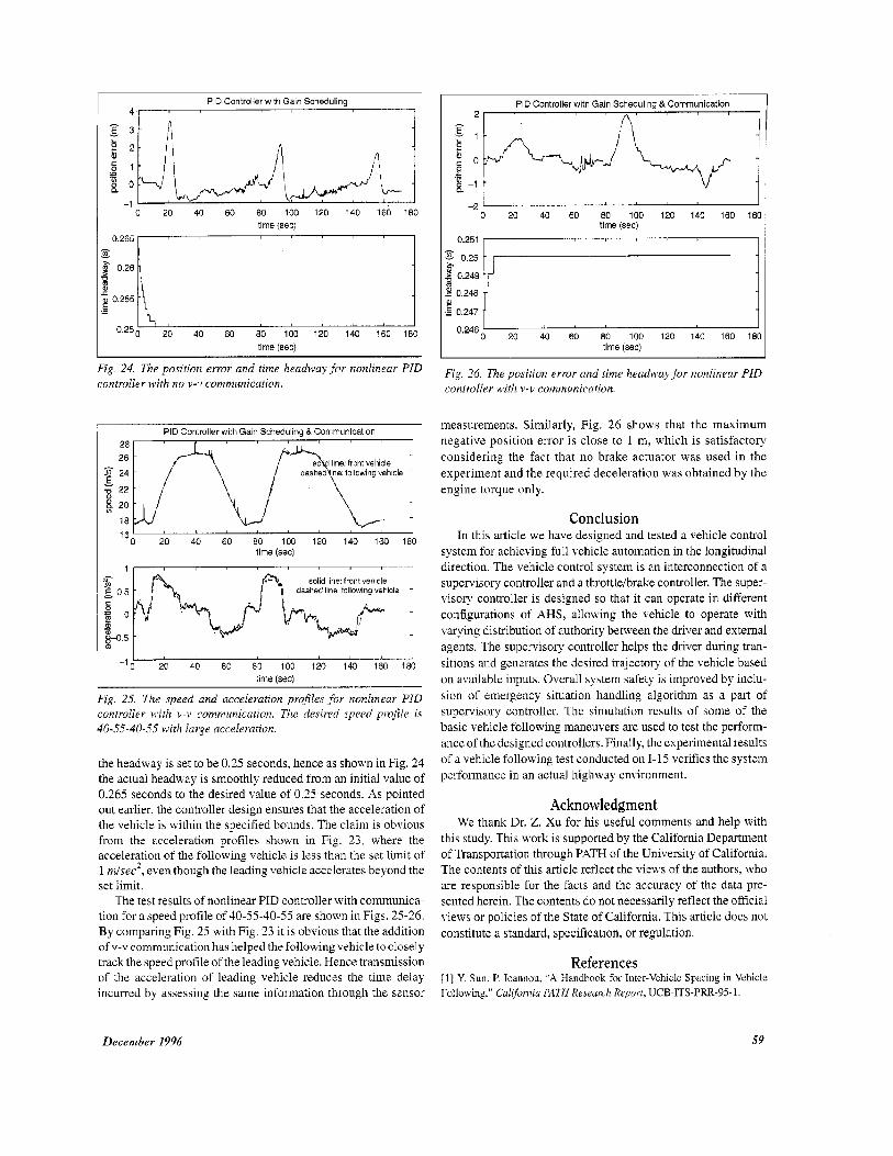
Fig. 23. The speed and acceleration profiles for nonlinear PID controller with no 11-11 cornm~mication. The desiredspeedprojle is 40-50-40-50 with large acceleration.

simplicity, we use 30-60-40-60 to indicate this speed profile. The second speed profile is 40-50-40-50 or 40-50 with large acceleration. The third speed profile is that the leading vehicle was driven manually following some sinusoidal speed curve. The results of only PID controller are included here, for a detailed description of this test conducted on 1-15 the reader is referred to [17].

The test results of nonlinear ?ID throttle controller and no v-v comnlunication are shown in Figs. 23-24. It can be seen from Fig. 21 that the negative position error is within 1 m, which allows the following vehicle to travel close to the leading vehicle without any collision. The speed profiles in Fig. 23 show that the following vehicle tracks the speed profile of the leading vehicle closely except near transitions. where a sudden change in speed of the leading vehicle creates a large position error, which is reduced by making the speed of the following vehicle greater thau that of the leading vehicle during that interval. In this test


PID Controiler with Gain Scheduling I

0 20 40 60 80 100 120 140 160 160 time (sec)

0.265 [

0.255

0'25/ ' 20 40 60 80 100 120 140 160 18; time (secj

L

Fig. 24. The position error and time headway for nonlinear PID controller with no v-v communication.

r PID Controller with Gain Scheduling & Communication

dashed ne. following vehicle so ' line: front vehlcle

8 20 16

I6O 20 40 60 80 100 120 140 160 180 time (sec)

dashed Ilne: following vehicle -

time (sec) L

Fig. 25. The speed and acceleration proJ1es for nonlinear PID controller with v-v communication. The desired speed profile is 40-55-40-55 with large acceleration.

the headway is set to be 0.25 seconds. hence as shown in Fig. 24 the actual headway is smoothly reduced from an initial value of 0.265 seconds to the desired value of 0.25 seconds. As pointed out earlier, the controller design ensures that the acceleration of the vehicle is within the specified bounds. The claim is obvious from the acceleration profiles shown in Fig. 23. where the acceleration of the following vehicle is less than the set limit of 1 ndsec2, even though the leading vehicle accelerates beyond the set limit.

The test results of nonlinear PID controller with communication for a speed profile of 40-55-40-55 are shown in Figs. 25-26. By comparing Fig. 25 with Fig. 23 it is obvious that the addition of v-v communication has helped the following vehicle to closely track the speed profile of the leading vehicle. Hence transmission of the acceleration of leading vehicle reduces the time delay incurred by assessing the same information through the sensor

PID Controller with Gain Scheduling &Communication

I 0 20 40 60 80 100 120 140 160 18C -c

time (secj I 0.251 I I '" 0.25

0.249

0.248

0.247

0'246: 20 40 6b EO 100 120 IbO 160 18; time (sec)

Fig. 26. The position error and time headway for nonlinear PID controller with 11-v communication.

measurements. Similarly, Fig. 26 shows that the maximum negative position error is close to 1 m, which is satisfactory considering the fact that no brake actuator was used in the experiment and the required deceleration was obtained by the engine torque only.

Conclusion In this article we have designed and tested a vehicle control

system for achieving full vehicle automation in the longitudinal direction. The vehicle control system is an interconnection of a supervisory controller and a throttlehrake controller. The supervisory controller is designed so that it can operate in different configurations of AHS, allowing the vehicle to operate with varying distribution of authority between the driver and external agents. The supervisory controller helps the driver during transitions and generates the desired trajectory of the vehicle based on available inputs. Overall system safety is improved by inclu- sion of emergency situation handling algorithm as a part of supervisory controller. The simulation results of some of the basic vehicle following maneuvers are used to test the performance ofthe designed controllers. Finally, the experimental results of a vehicle following test conducted on 1-15 verifies the system performance in an actual highway environment.

Acknowledgment We thank Dr. Z. Xu for his useful comments and help with

this study. This work is supported by the California Department of Transportation through PATH of the University of California. The contents of this article reflect the views of the authors, who are responsible for the facts and the accuracy of the data presented herein. The contents do not necessarily reflect the official views or policies ofthe State of California. This article does not constitute a standard, specification, or regulation.

References [ I ] Y. Sun. P. Ioannou, "A Handbook for Inter-Vehicle Spacing in Vehicle Following." Californiu PATH Research Report, UCB-ITS-PRR-95-1.

December 1996 59

[2] D.B. Maciuca, J.K. Hedrick, “Brake Dynamics Effect on AHS Lane Capacity.“ Sysrems und 2Y.ures i n ITS, Society of Automotive Engineers. Warrandale, P.%, pp. 81-86, 1995.

[3] V. Sarakki, J. Kerr, “Effectiveazss of IVHS Elements on Freex a) /Arterial Capacity: Concepts and Case Studies,” 64th Meeting of Institute of Trans- portation Engineers. Dallas, Compendium <f Teciuzical Pupers. Institute of Transportation Engineers, Washington D.C., pp. 303-307, 1991.

[4] M. Shannon, et al.. “Precursor Systems Analyses of Automated Highuaq Systems: .4HS Safety Issues,” vol. 9, Federal Highway Adminlstration, Washington D.C.. Report KO. FHUR-RD-95-105. 1995.

[5] A. Hitchcock, “Configuration and Maneuvers in Safety-Consciously Designed AHS Configuration;” California PATH Program. University of California at Berkeley: UCB-ITS-PWP-95-2, 1995.

[6] K.S. Chang, J.K. Hedrick. W.B. Zhang. P. Varaiya, M. Tomizuka. S.E. Shladover, ’:4utomated Highway System Experiments in the P,%TH Pro- gram.” IL’HS Jouwd. vol 1. no. 1. pp. 63-87. April 1993.

[7] C.C. Chien. P. Ioannou, “.4utomatic Vehicle Following,” Proc. of1992 American Conrroi Confeiance, Chicago. IL. pp. 1748-1752. June 1992.

[8] J.K. Hednck, et. al, ”Control Issues in Automated Highway Systems:” E E E Control Systems. vol. 14, no. 6; pp. 21-32, December 1994.

[9] P. Ioannou, C.C. Chen, ”Intelligent Cruise Control,” IEEE Transactions on Vehiculur Technolog!. vol. 42, no. 4, pp. 657-672, November 1993.

[lo] P. Ioannou, 2. Xu, ”Throttle and Brake Control System for Automatic Vzhicle Following.” II’HS Journal. vol. 1(1), pp. 345-377, 1994.

[ll] S.E. Shladover, et al., ‘:4utomatic Vehicle Control Developments in the PATH Program,” IEEE Ti-umactiorrs on Vehicular Technolog), vol. 40. no. 1. pp. 114-130, February 1993.

[l?] C.C. Chien. Y. Zhang. X. Stotskq, S.R. Dharmasena, P. Ioannou. “Mac- roscopic Roadway Traffic Controller Design,’’ California R4TH Reseaxh Report, UCB-ITS-PRR-95-28.

1131 P. Varaiya, “Smart Cars on Smart Roads: Problems of Control,” IEEE Tranractions on Autornntic Control, vol. 38, no. 2. pp. 195-207, February 1993.

[14] J.K Hedrick, D. McMahon, V Narendran, D. Sararoop, “Longitudinal Vehicle Controller Design for IVHS System.” Proc. of ACC. vol. 3. pp. 3107-3112, June 1991.

[ 151 A S . Hauksdottir, R.E. Fenton, “On the Design of aVeh1cle Longitudinal Controller,” IEEE Trmzs. oil Vehicular Teclmologj, vol. VT-34, no. 4. pp. 182-187, November 1985.

1161 WA. Coppel, ‘Stability and Asymptotic Behavior of Differential Equa- tions,“ D.C. Heath and Company. Boston, pp. 61-70. 1965.

1171 P. Ioannou, Z. Xu, H. Raza. “Report on 1-15 Vehicle Following Test,” USC-CATI Report 1196-3-01

Humair Raza recehed the B.S. degree in electrical engineering from the University of Engineering and Technology, Lahore. Pakistan. He received the M.S. degree in electrical engineering from the University of Southern Califoria, Los Angeles. where he is currently a Ph.D. candidate. His research interests include adaptive control. fuzzy control, modeling and control of advanced vehicle control systems.

Petros 4. Ioannou received the BSc. degree with First Class Honors from University College, London. Eng- land. in 1978 and the M S . and Ph.D. degrees from the University of Illinois. Urbana, Illinois. in 1980 and 1982, respectively. In 1982, Dr. Ioannou joined the Department of Electrical Engineering-Systems, Uni- versity of Southern California, Los Angeles, California where he is currently a professor and the director of the Center of Advanced Transportation Technologies. His

research interests are in adaptive control and applications, intelligent transportation systems, vehicle dynamics and control and neural networks. Dr. Ioannou is a fellow of IEEE.


vehicle following control design for automated …ioannou/2003update/d50.pdfvehicle following...

Documents