vel. diagrams

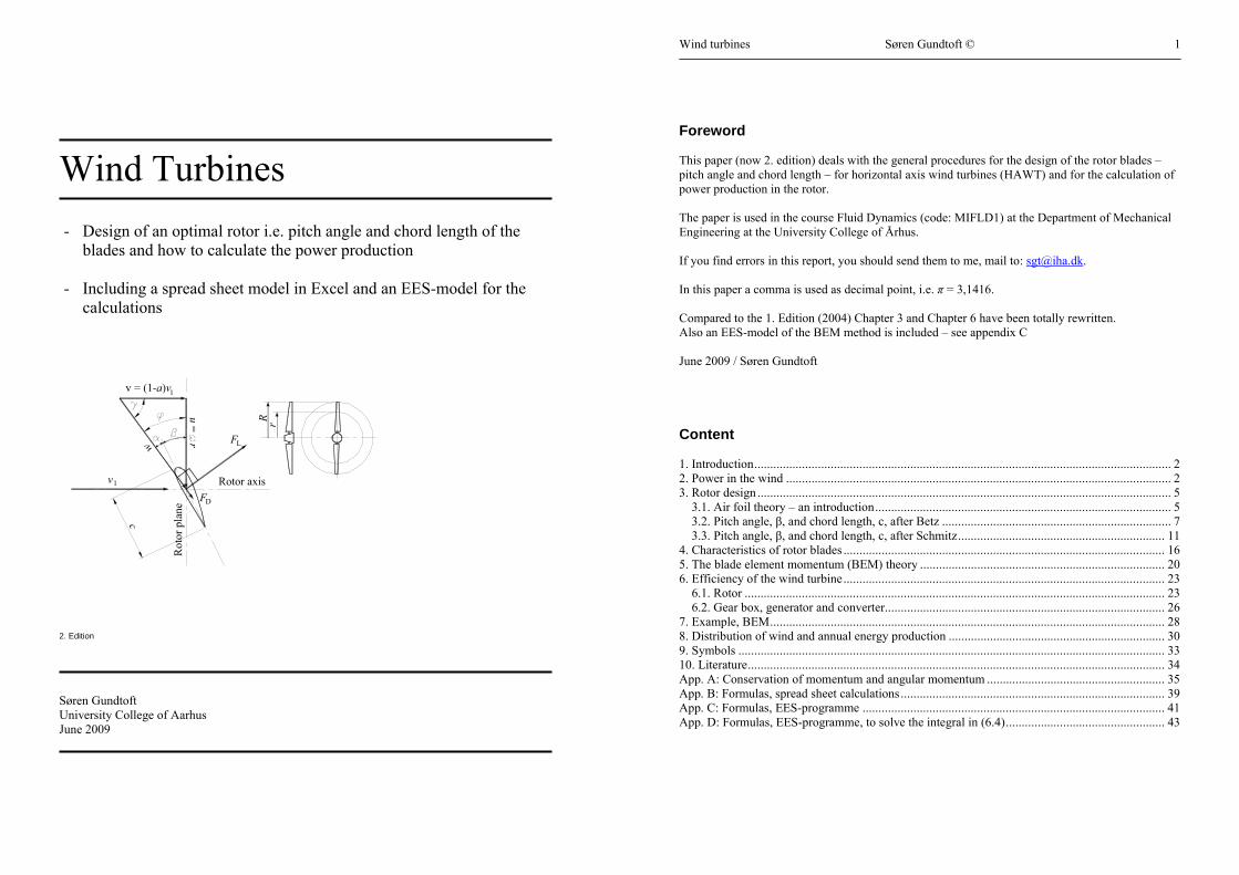
Wind Turbines - Design of an optimal rotor i.e. pitch angle and chord length of the

blades and how to calculate the power production - Including a spread sheet model in Excel and an EES-model for the

calculations

r

Rotor axis

FL

DF

1v = (1-a)v

v1

w

Rot

or p

lan e

u = rR

c

2. Edition

Søren Gundtoft University College of Aarhus June 2009

Wind turbines Søren Gundtoft © 1

Foreword This paper (now 2. edition) deals with the general procedures for the design of the rotor blades – pitch angle and chord length – for horizontal axis wind turbines (HAWT) and for the calculation of power production in the rotor. The paper is used in the course Fluid Dynamics (code: MIFLD1) at the Department of Mechanical Engineering at the University College of Århus. If you find errors in this report, you should send them to me, mail to: [email protected]. In this paper a comma is used as decimal point, i.e. π = 3,1416. Compared to the 1. Edition (2004) Chapter 3 and Chapter 6 have been totally rewritten. Also an EES-model of the BEM method is included – see appendix C June 2009 / Søren Gundtoft Content 1. Introduction................................................................................................................................... 2 2. Power in the wind ......................................................................................................................... 2 3. Rotor design .................................................................................................................................. 5

3.1. Air foil theory – an introduction............................................................................................. 5 3.2. Pitch angle, β, and chord length, c, after Betz ........................................................................ 7 3.3. Pitch angle, β, and chord length, c, after Schmitz................................................................. 11

4. Characteristics of rotor blades ..................................................................................................... 16 5. The blade element momentum (BEM) theory ............................................................................. 20 6. Efficiency of the wind turbine..................................................................................................... 23

6.1. Rotor .................................................................................................................................... 23 6.2. Gear box, generator and converter........................................................................................ 26

7. Example, BEM............................................................................................................................ 28 8. Distribution of wind and annual energy production .................................................................... 30 9. Symbols ...................................................................................................................................... 33 10. Literature................................................................................................................................... 34 App. A: Conservation of momentum and angular momentum ........................................................ 35 App. B: Formulas, spread sheet calculations................................................................................... 39 App. C: Formulas, EES-programme ............................................................................................... 41 App. D: Formulas, EES-programme, to solve the integral in (6.4).................................................. 43


1. Introduction It is assumed that the reader knows some basic fluid mechanics, for example the basic theories of fluid properties, the ideal gas law, Bernoulli’s equation, turbulent and laminar flow, Reynolds’s number, etc. Important for the understanding of the theory is mastering the conservation laws for momentum and angular momentum, for which reason these theories are presented in Appendix A. In this paper you will find: • Chapter 2: How much energy that can be taken from the wind in an idealized wind turbine

(proof of Betz’ law) and how to design the rotor • Chapter 3: How to design a an optimal rotor – pitch angle and chord length • Chapter 4: Characteristic of rotor blades (coefficients of lift and drag) • Chapter 5: How to calculate the power of a given rotor (the BEM theory) • Chapter 6: Efficiency of a wind turbine • Chapter 7: An example – BEM method in Excel • Chapter 8: Distribution of the natural wind and calculation of annual energy production Most of the theory is taken from ref./1/ and /4/. Data for rotor blade sections are taken from ref./2/ and /3/. All important calculations are demonstrated by examples. The calculations after the BEM method can be done by simple spread sheet calculations and in Appendix B the formulas are printed. Also the code for an EES-model of the BEM method is presented, see Appendix C.

2. Power in the wind The question is: How much energy can be taken from the wind? The wind turbine decelerates the wind, thereby reducing the kinetic energy in the wind. But the wind speed cannot be reduced to zero – as a consequence, where should the air be stored? As first time shown by Betz, there is an optimum for the reduction of the wind speed, and this is what is to be outlined in this chapter. Figure 2.1 shows the streamlines of air through a wind turbine Notation: In the following we will use index 1 for states “far up stream” the rotor plane, index for the states in the rotor plane and index 3 for states far downstream. For simplicity index 2 – states in the rotor plane - will be omitted in most cases. Long in front of the rotor, the wind speed is v1. After passing the wind turbine rotor (called the rotor in the following), the wind speed would be reduced to v3. The pressure distribution is as follows. The initial pressure is p1. As the air moves towards the rotor, the pressure rises to a pressure p+ and by passing the rotor, the pressure suddenly falls by an amount of ∆p i.e. the pressure is here p- = p+ - ∆p. After passing the rotor, and far down stream the pressure again rises to p3 = p1. Curves for wind speed and pressure are shown in figure 2.1. Bernoulli’s equation: If we look at the air moving towards the rotor plane, we can use the Bernoulli’s equation to find the relation between the pressure p and the speed v, while we can make the assumption that the flow is frictionless:


tot2

21 ppv =+ρ [Pa] (2.1)

where ptot is the total pressure, which is constant. That means, if the speed of flow goes up, the pressure goes down and vice versa.

1v1v

v 3

A3AA1

p1 p3 =p1p

p - p

v1v

v 3Spee

dPr

essu

re

Figure 2.1: Interaction between wind and wind turbine Assumption: The pressure changes are relatively small compared to the pressure in the ambient (about 1 atm = 101325 Pa) therefore we assume the density to be constant. If we use (2.1) for the flow up-stream of the rotor, we get

2211 2

121 vpvp ρρ +=+ + [Pa] (2.2)

If we use (2.1) down stream of the rotor plane, we get

231

2

21

21 vpvpp ρρ +=+∆−+ [Pa] (2.3)

Subtracting (2.3) from (2.2) we get

( )23

212

1 vvp −=∆ ρ [Pa] (2.4)

Change of momentum: This differential pressure can also be calculated on the basis of”change in momentum”. (For information see Appendix A). If we look at one square meter of the rotor plane,


the mass flow equals ρ v. Momentum equals mass times velocity, with the unit N. Pressure equals force per surface, then the differential pressure can be calculated as

( )31 vvvp −=∆ ρ [Pa] (2.5) Now (2.4) and (2.5) give

( )3121 vvv += [m/s] (2.6)

This indicates that the speed of air in the rotor plane equals the mean value of the speed upstream and down stream of the rotor. Power production: The power of the turbine equals the change in kinetic energy in the air

( )AvvvP 23

212

1−= ρ [W] (2.7)

Here A is the surface area swept by the rotor. The axial force (thrust) on the rotor can be calculated as

ApT ∆= [N] (2.8) We now define ”the axial interference factor” a such that

( ) 11 vav −= [m/s] (2.9) Using (2.6) and (2.9) we get v3 = (1 – 2a) v1 and (2.7) and (2.8) can be written as

( ) AvaaP 31

212 −= ρ [W] (2.10)

( ) AvaaT 2112 −= ρ [N] (2.11)

We now define two coefficients, one of the power production and one of the axial forces as

( )2P 14 aaC −= [-] (2.12)

( )aaC −= 14T [-] (2.13)

Then (2.10) and (2.11) can be written as

P3

121 CAvP ρ= [W] (2.14)


T2

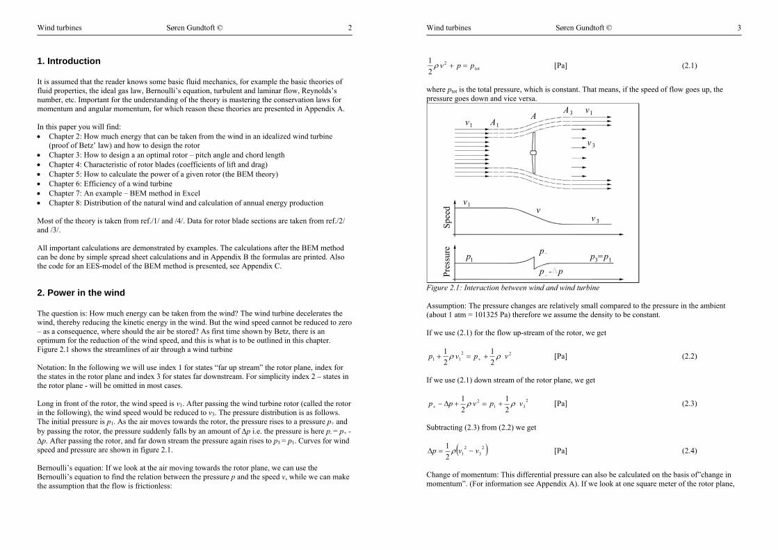
1½ CAvT ρ= [N] (2.15) In figure 2.2, curves for CP and CT are shown.

0,0

0,2

0,4

0,6

0,8

1,0

0 0,1 0,2 0,3 0,4 0,5

a [-]

C_P

& C

_T [-

]

C_T

C_P

=16/27

Figure 2.2: Coefficient of power CP and coefficient of axial force CT for an idealized wind turbine. As shown, CP has an optimum at about 0,593 (exactly 16/27) at an axial interference factor of 0,333 (exactly 1/3). According to Betz we have

2716with½ BetzP,

31Betzp,Betz == CAvCP ρ [W] (2.16)

Example 2.1 Let us compare the axial force on rotor to the drag force on a flat plate? If a = 1/3 the CT = 8/9 ≈ 0,89. Wind passing a flat plate with the area A would give a drag on the plate of

AvCF 21DD 2

1 ρ= [N] (2.17)

where CD ≈ 1,1 i.e. the axial force on at rotor – at maximal power – is about 0,89/1,1 = 0,80 = 80% of the force on a flat plate of the same area as the rotor!

3. Rotor design

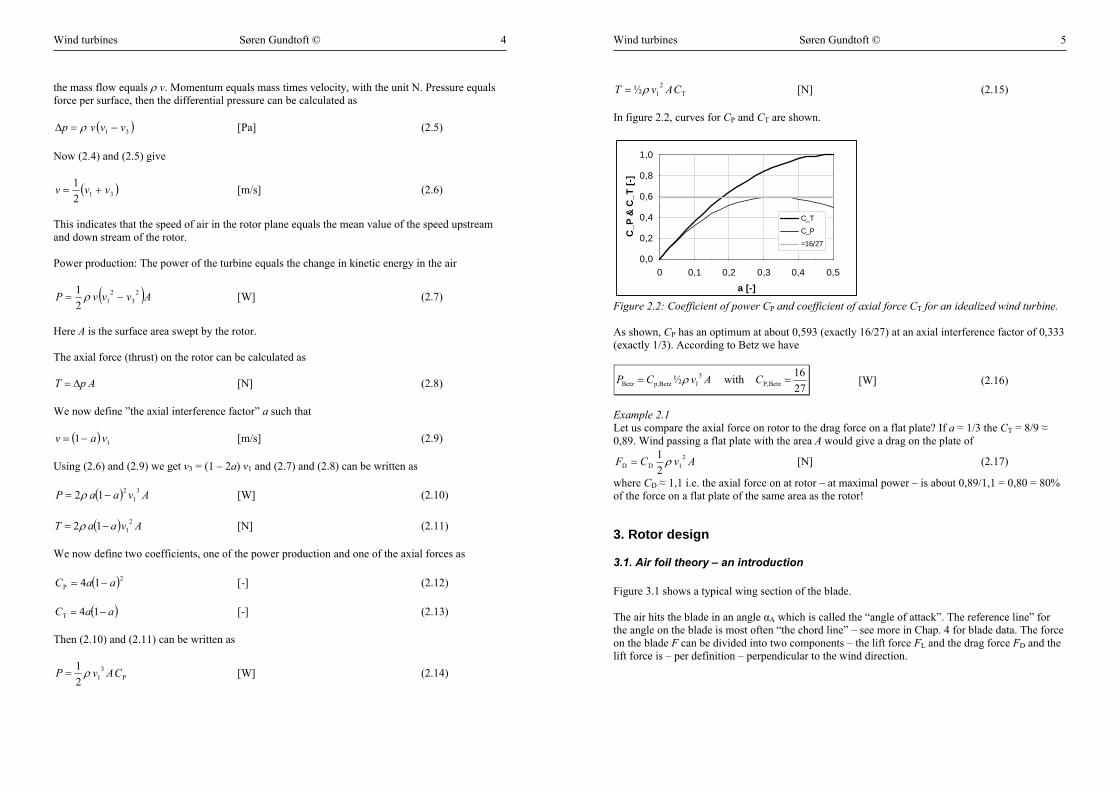
3.1. Air foil theory – an introduction Figure 3.1 shows a typical wing section of the blade. The air hits the blade in an angle αA which is called the “angle of attack”. The reference line” for the angle on the blade is most often “the chord line” – see more in Chap. 4 for blade data. The force on the blade F can be divided into two components – the lift force FL and the drag force FD and the lift force is – per definition – perpendicular to the wind direction.


FD

w

LFF

Chord line

Figure 3.1: Definition of angle of attack The lift force can be calculated as

( )cbwCF 2LL 2

1 ρ= (3.1)

where CL is the “coefficient of lift”, ρ is the density of air, w the relative wind speed, b the width of the blade section and c the length of the chord line. Similar for the drag force

( )cbwCF 2DD 2

1 ρ= (3.2)

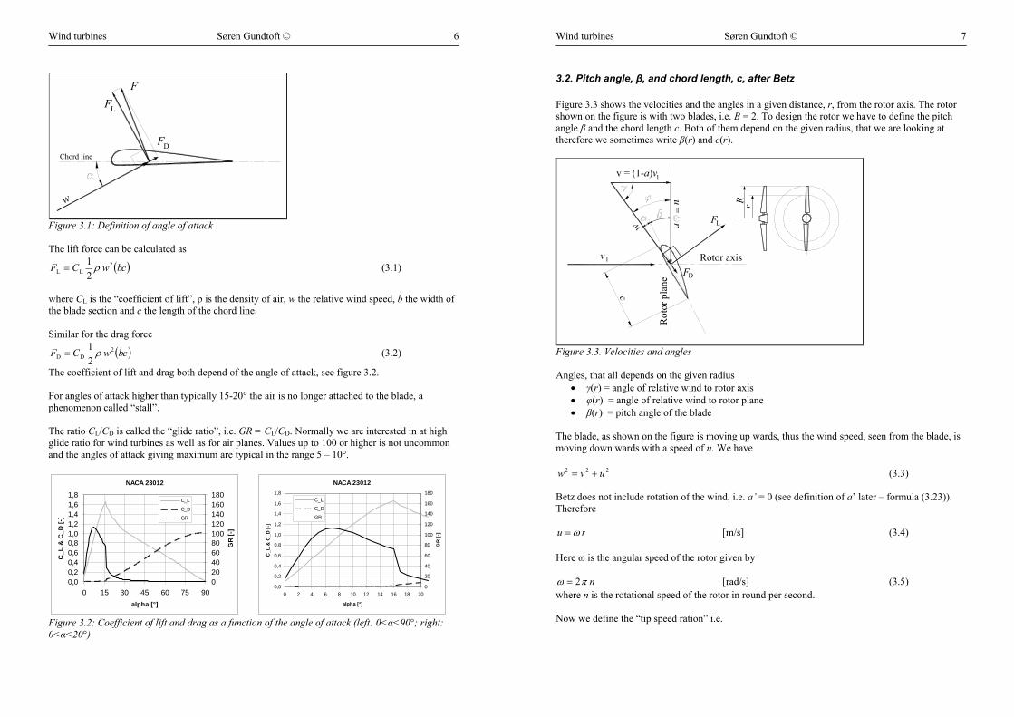
The coefficient of lift and drag both depend of the angle of attack, see figure 3.2. For angles of attack higher than typically 15-20° the air is no longer attached to the blade, a phenomenon called “stall”. The ratio CL/CD is called the “glide ratio”, i.e. GR = CL/CD. Normally we are interested in at high glide ratio for wind turbines as well as for air planes. Values up to 100 or higher is not uncommon and the angles of attack giving maximum are typical in the range 5 – 10°.

NACA 23012

0,00,20,40,60,81,01,21,41,61,8

0 15 30 45 60 75 90alpha [°]

C_L

& C

_D [-

]

020406080100120140160180

GR

[-]

C_L

C_D

GR

NACA 23012

0,0

0,2

0,4

0,6

0,8

1,0

1,2

1,4

1,6

1,8

0 2 4 6 8 10 12 14 16 18 20

alpha [°]

C_L

& C

_D [-

]

0

20

40

60

80

100

120

140

160

180

GR

[-]

C_L

C_D

GR

Figure 3.2: Coefficient of lift and drag as a function of the angle of attack (left: 0<α<90°; right: 0<α<20°)


3.2. Pitch angle, β, and chord length, c, after Betz Figure 3.3 shows the velocities and the angles in a given distance, r, from the rotor axis. The rotor shown on the figure is with two blades, i.e. B = 2. To design the rotor we have to define the pitch angle β and the chord length c. Both of them depend on the given radius, that we are looking at therefore we sometimes write β(r) and c(r).

r

Rotor axis

FL

DF

1v = (1-a)v

v1

w

Rot

or p

lane

u = rR

c

Figure 3.3. Velocities and angles Angles, that all depends on the given radius

• γ(r) = angle of relative wind to rotor axis • φ(r) = angle of relative wind to rotor plane • β(r) = pitch angle of the blade

The blade, as shown on the figure is moving up wards, thus the wind speed, seen from the blade, is moving down wards with a speed of u. We have

222 uvw += (3.3) Betz does not include rotation of the wind, i.e. a’ = 0 (see definition of a’ later – formula (3.23)). Therefore

ru ω= [m/s] (3.4) Here ω is the angular speed of the rotor given by

nπω 2= [rad/s] (3.5) where n is the rotational speed of the rotor in round per second. Now we define the “tip speed ration” i.e.


11

tip

vR

vv

X ω== [-] (3.6)

Combining these equations we get

( )RXrr

23arctan=γ [rad] (3.7)

or

( )XrRr

32arctan=ϕ [rad] (3.8)

and then the pitch angle

( ) DBetz 32arctan αβ −=

XrRr [rad] (3.9)

where αD is the angle of attack, used for the design of the blade. Most often the angle is chosen to be close to the angle, that gives maximum glide ration, see figure 3.2 that means in the range from 5 to 10°, but near the tip of the blade the angle is sometimes reduced.

Chord length, c(r): If we look at one blade element in the distance r from the rotor axis with the thickness dr the lift force is, see formula (3.1) and (3.2)

L2

L d21d CrcwF ρ= [N] (3.10)

and the drag force

D2

D d21d CrcwF ρ= [N] (3.11)

r R

dr

Figure 3.4: Blade section


Rotor axis

Rot

or p

lane D

dF

dFL

LdU

dUD D

dF

LdFdFL

DdF

dTL

dTD

Torque Thrustx

y12.07.2008/SGt

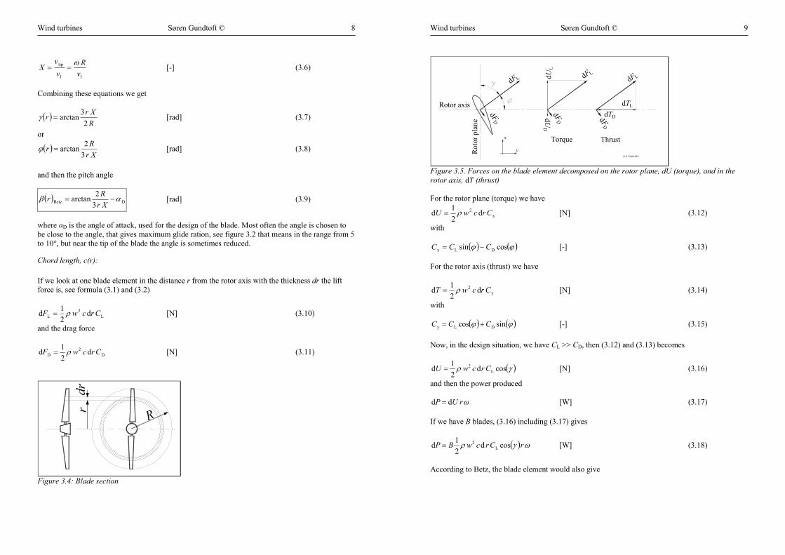
Figure 3.5. Forces on the blade element decomposed on the rotor plane, dU (torque), and in the rotor axis, dT (thrust) For the rotor plane (torque) we have

x2 d

21d CrcwU ρ= [N] (3.12)

with

( ) ( )ϕϕ cossin DLx CCC −= [-] (3.13) For the rotor axis (thrust) we have

y2 d

21d CrcwT ρ= [N] (3.14)

with

( ) ( )ϕϕ sincos DLy CCC += [-] (3.15) Now, in the design situation, we have CL >> CD, then (3.12) and (3.13) becomes

( )γρ cosd21d L

2 CrcwU = [N] (3.16)

and then the power produced

ωrUP dd = [W] (3.17) If we have B blades, (3.16) including (3.17) gives

( ) ωγρ rCrcwBP cosd21d L

2= [W] (3.18)

According to Betz, the blade element would also give


( )rrvP d221

2716d 3

1 πρ= [W] (3.19)

Using v1 = 3/2 w cos(γ) and u = w sin(γ), then (3.18) and (3.19) gives

( )

94

1916

22DL,

Betz

+⎟⎠⎞

⎜⎝⎛

=

RrXX

CBRrc π

[m] (3.20)

where CL,D is the coefficient of lift at the chosen design angle of attack, αA,D.

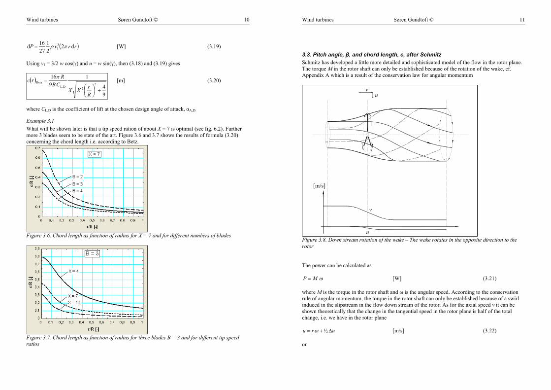
Example 3.1 What will be shown later is that a tip speed ration of about X = 7 is optimal (see fig. 6.2). Further more 3 blades seem to be state of the art. Figure 3.6 and 3.7 shows the results of formula (3.20) concerning the chord length i.e. according to Betz.

Figure 3.6. Chord length as function of radius for X = 7 and for different numbers of blades

Figure 3.7. Chord length as function of radius for three blades B = 3 and for different tip speed ratios


3.3. Pitch angle, β, and chord length, c, after Schmitz Schmitz has developed a little more detailed and sophisticated model of the flow in the rotor plane. The torque M in the rotor shaft can only be established because of the rotation of the wake, cf. Appendix A which is a result of the conservation law for angular momentum

v

vu

u

[m/s]

Figure 3.8. Down stream rotation of the wake – The wake rotates in the opposite direction to the rotor The power can be calculated as

ωMP = [W] (3.21) where M is the torque in the rotor shaft and ω is the angular speed. According to the conservation rule of angular momentum, the torque in the rotor shaft can only be established because of a swirl induced in the slipstream in the flow down stream of the rotor. As for the axial speed v it can be shown theoretically that the change in the tangential speed in the rotor plane is half of the total change, i.e. we have in the rotor plane

uru ∆+= ½ω [m/s] (3.22) or


( )'1 aru += ω [m/s] (3.23)

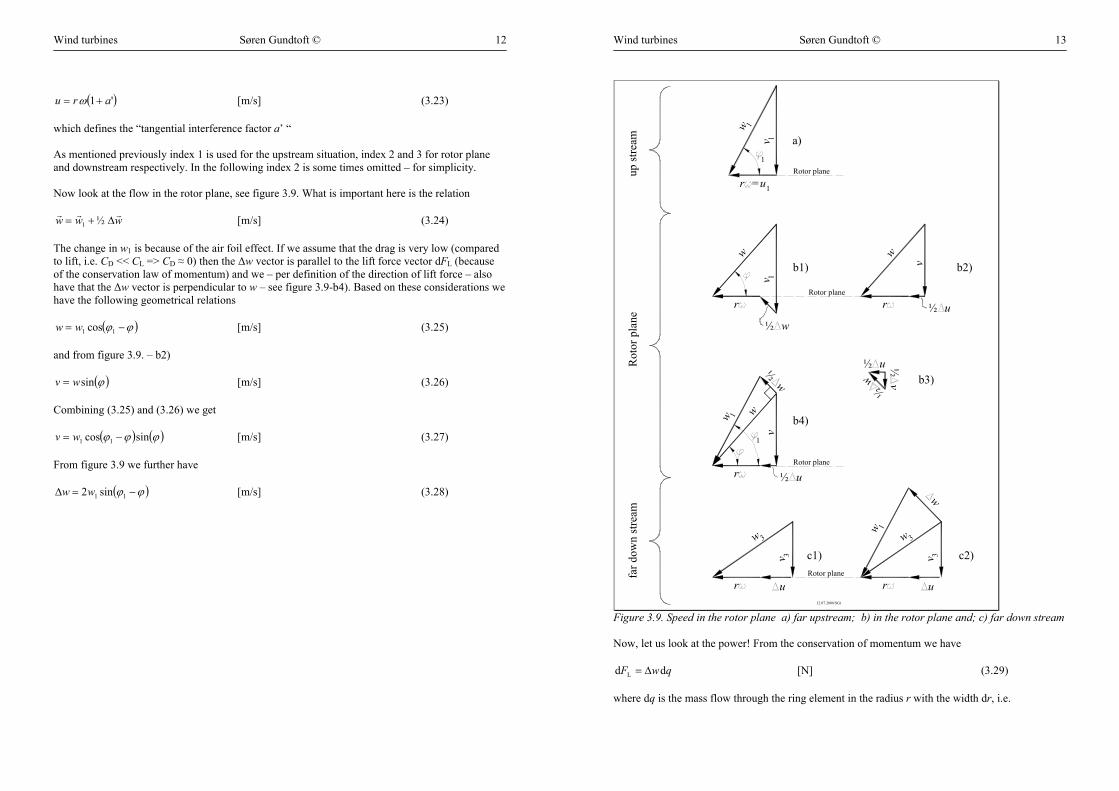
which defines the “tangential interference factor a’ “ As mentioned previously index 1 is used for the upstream situation, index 2 and 3 for rotor plane and downstream respectively. In the following index 2 is some times omitted – for simplicity. Now look at the flow in the rotor plane, see figure 3.9. What is important here is the relation

www rrr∆+= ½1 [m/s] (3.24)

The change in w1 is because of the air foil effect. If we assume that the drag is very low (compared to lift, i.e. CD << CL => CD ≈ 0) then the ∆w vector is parallel to the lift force vector dFL (because of the conservation law of momentum) and we – per definition of the direction of lift force – also have that the ∆w vector is perpendicular to w – see figure 3.9-b4). Based on these considerations we have the following geometrical relations

( )ϕϕ −= 11 cosww [m/s] (3.25) and from figure 3.9. – b2)

( )ϕsinwv = [m/s] (3.26) Combining (3.25) and (3.26) we get

( ) ( )ϕϕϕ sincos 11 −= wv [m/s] (3.27) From figure 3.9 we further have

( )ϕϕ −=∆ 11 sin2ww [m/s] (3.28)


w 1

1v

1=u

1

r

1v

r

w

½ w

w

r

v

u½

½ u

w½

½v

v

r

w

½ u

1w

1

w½

v 3

r

w 3

u

Rot

or p

lan e

far d

own

stre

amup

str e

am a)

b1)

b4)

c1)

b2)

b3)

Rotor plane

Rotor plane

Rotor plane

Rotor plane

12.07.2008/SGt

1

r

w

w

v

u

3

3

w

c2)

Figure 3.9. Speed in the rotor plane a) far upstream; b) in the rotor plane and; c) far down stream Now, let us look at the power! From the conservation of momentum we have

qwF dd L ∆= [N] (3.29) where dq is the mass flow through the ring element in the radius r with the width dr, i.e.


vrrq d2d πρ= [kg/s] (3.30)

Power equals “torque multiplied by angular velocity” and (neglecting drag) then

( )( )( ){ }( ) ( ) ( )[ ] ( )

( )[ ] ( )12

121

21111

L

sin2sind2

sinsincosd2sin2sind

sinddd

ϕϕϕπρω

ωϕϕϕϕπρϕϕωϕ

ωϕω

−=

−−=∆=

==

wrrrwrrw

rqwrF

MP

[kg/s] (3.31)

In the bottom transaction above we have used the relation sin(x) cos(x) = sin(2x). We have now a relation for the power of the ring element as a function of the angle φ but we do not know this angle? The trick is now to solve the equation d(dP)/dφ = 0 to find the angle that gives maximum power. Doing this for (3.31) we get ( ) ( ) ( )[ ] ( )[ ]( )

( ) ( )[ ] ( )[ ]{ }( ) ( ){ }ϕϕϕπρω

ϕϕϕϕϕϕπρω

ϕϕϕϕϕϕϕπρωϕ

32sinsin2d2

sin2coscos2sinsin2d2

cossin2sin2sin2cos2d2ddd

121

211

21

2

12

121

2

−=

−−−=

−+−−=

wrr

wrr

wrrP

[W/°] (3.32)

From d(dP)/dφ = 0, it follows

1max 32ϕϕ = [rad] (3.33)

or

rXR

rv arctan

32arctan

32 1

max ==ω

ϕ [rad] (3.34)

and the for pitch angle

( ) DSchmitz arctan32 αβ −=

XrRr [rad] (3.35)

Example 3.2

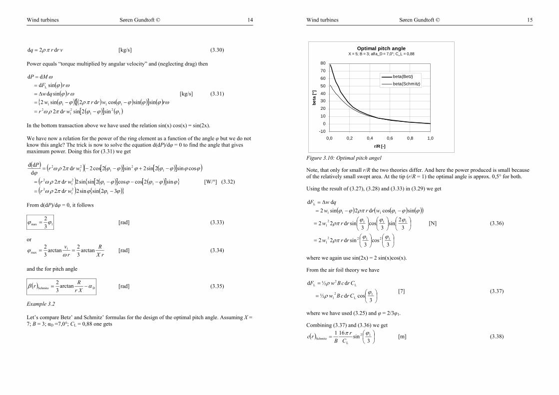
Let’s compare Betz’ and Schmitz’ formulas for the design of the optimal pitch angle. Assuming X = 7; B = 3; αD =7,0°; CL = 0,88 one gets


Optimal pitch angleX = 5; B = 3; alfa_D = 7,0°; C_L = 0,88

-10

0

10

20

30

40

50

60

70

80

0,0 0,2 0,4 0,6 0,8 1,0

r/R [-]

beta

[°]

beta(Betz)

beta(Schmitz)

Figure 3.10: Optimal pitch angel

Note, that only for small r/R the two theories differ. And here the power produced is small because of the relatively small swept area. At the tip (r/R = 1) the optimal angle is approx. 0,5° for both.

Using the result of (3.27), (3.28) and (3.33) in (3.29) we get

( ) ( ) ( )( )

⎟⎠⎞

⎜⎝⎛

⎟⎠⎞

⎜⎝⎛=

⎟⎠⎞

⎜⎝⎛

⎟⎠⎞

⎜⎝⎛

⎟⎠⎞

⎜⎝⎛=

−−=∆=

3cos

3sind22

32

sin3

cos3

sind22

sincosd2sin2dd

121221

11121

1111

L

ϕϕρπ

ϕϕϕρπ

ϕϕϕρπϕϕ

rrw

rrw

wrrwqwF

[N] (3.36)

where we again use sin(2x) = 2 sin(x)cos(x).

From the air foil theory we have

⎟⎠⎞

⎜⎝⎛=

=

3cosd½

d½d

1L

21

L2

L

ϕρ

ρ

CrcBw

CrcBwF [7] (3.37)

where we have used (3.25) and φ = 2/3φ1.

Combining (3.37) and (3.36) we get

( ) ⎟⎠⎞

⎜⎝⎛=

3sin161 12

LSchmitz

ϕπC

rB

rc [m] (3.38)


or

( ) ⎟⎟⎠

⎞⎜⎜⎝

⎛⎟⎟⎠

⎞⎜⎜⎝

⎛=

rXR

Cr

Brc arctan

31sin161 2

LSchmitz

π [m] (3.39)

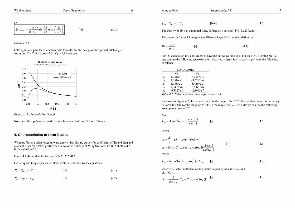
Example 3.3

Let’s again compare Betz’ and Schmitz’ formulas for the design of the optimal pitch angle. Assuming X = 7; B = 3; αD =7,0°; CL = 0,88 one gets

Optimal chord ratioX = 5; B = 3; alfa_D = 7,0°; C_L = 0,88

0,00,10,20,30,40,50,60,7

0,0 0,2 0,4 0,6 0,8 1,0

r/R [-]

c/R

[-]

c/R(Betz)

c/R(Schmitz)

Figure 3.11: Optimal chord length Note, near the tip there are no difference between Betz’ and Schmitz’ theory.

4. Characteristics of rotor blades Wing profiles are often tested in wind tunnels. Results are curves for coefficient of lift and drag and moment. Data for a lot of profiles can be found in ”Theory of Wing Sections, Ira H. Abbott and A. E. Doenhoff, ref./3/. Figure 4.1 shows data for the profile NACA 23012. Lift, drag and torque (per meter blade width) are defined by the equations

L2*

L ½ CcwF ρ= [N] (4.1)

D2*

D ½ CcwF ρ= [N] (4.2)


M22*

M ½ CcwQ ρ= [Nm] (4.3) The density of air is at a nominal state, defined as 1 bar and 11°C, 1,225 kg/m3. The curves in figure 4.1 are given at different Reynolds’s number, defined as

ρµ /Re wc

= [-] (4.4)

For PC-calculation it is convenient to have the curves as functions. For the NACA 23012 profile one can use the following approximation: CD,L = k0 + k1α + k2α2 + k3α3 + k4α4, with the following constants

NACA 23012 CL CD k0 k1 k2 k3 k4

1,0318e-1 1,0516e-1 1,0483e-3 7,3487e-6 –6,5827e-6

6,0387e-3 –3,6282e-4 5,4269e-5 6,5341e-6 –2,8045e-7

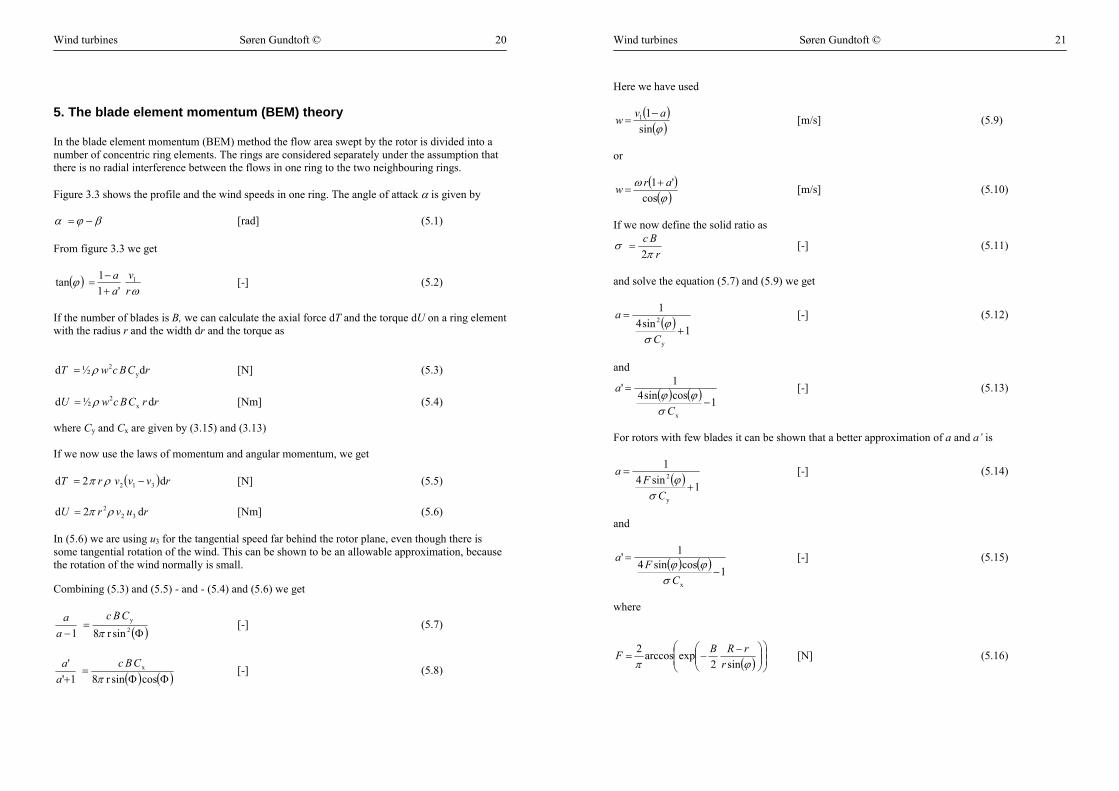
Table 4.1: Polynomial constants – for 0 < α < 16° As shown in figure 4.2, the data are given in the range of α < 20°. For wind turbines it is necessary to know the data for the range up to 90°. In the range from αst <α < 90° we can use the following assumptions, see ref./2/ Lift:

( ) ( )( )ααα

sincos2sin

2

21L AAC += [-] (4.5)

where

( ) ( )( ) ( )( )st

2st

ststmax,Ls2

11

1

cossincossin

)below! (4.8) see(2

ααααDCCA

BBA

−=

= [-] (4.6)

Drag:

( ) ( ) Ds22

1D cossin CBBC ++= αα [-] (4.7) where CDs is the coefficient of drag at the beginning of stall, αstall, and

( ) ( )( )st2

maxD,Dsst

2

maxD,1

sincos

1 αα

CCB

CB

−=

= [-] (4.8)


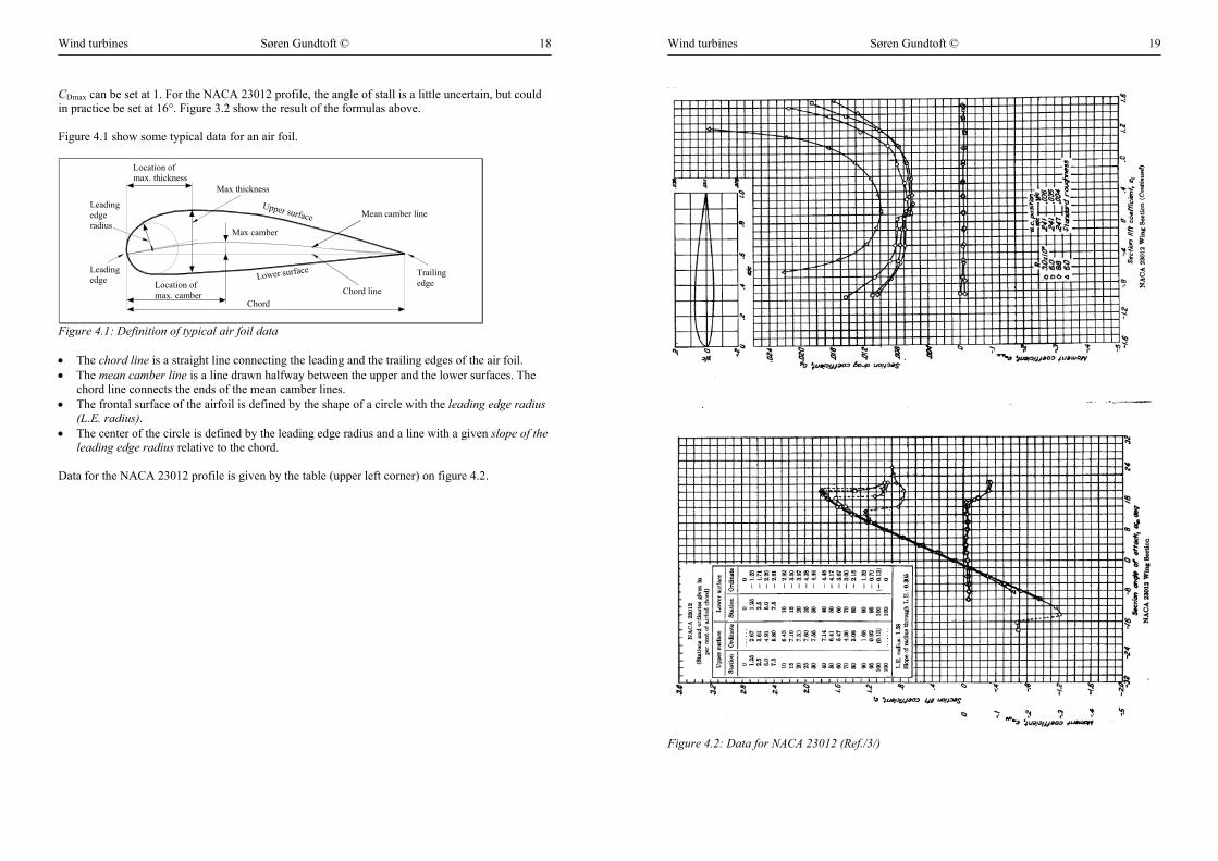
CDmax can be set at 1. For the NACA 23012 profile, the angle of stall is a little uncertain, but could in practice be set at 16°. Figure 3.2 show the result of the formulas above. Figure 4.1 show some typical data for an air foil.

Location of max. camber

Chord

Max camber

Mean camber lineUpper surface

Lower surface

Location of max. thickness

Max thickness

Leading edge

Trailing edge

Chord line

Leading edge radius

Figure 4.1: Definition of typical air foil data • The chord line is a straight line connecting the leading and the trailing edges of the air foil. • The mean camber line is a line drawn halfway between the upper and the lower surfaces. The

chord line connects the ends of the mean camber lines. • The frontal surface of the airfoil is defined by the shape of a circle with the leading edge radius

(L.E. radius). • The center of the circle is defined by the leading edge radius and a line with a given slope of the

leading edge radius relative to the chord. Data for the NACA 23012 profile is given by the table (upper left corner) on figure 4.2.


Figure 4.2: Data for NACA 23012 (Ref./3/)


5. The blade element momentum (BEM) theory In the blade element momentum (BEM) method the flow area swept by the rotor is divided into a number of concentric ring elements. The rings are considered separately under the assumption that there is no radial interference between the flows in one ring to the two neighbouring rings. Figure 3.3 shows the profile and the wind speeds in one ring. The angle of attack α is given by

βϕα −= [rad] (5.1) From figure 3.3 we get

( )ω

ϕrv

aa 1

'11tan+−

= [-] (5.2)

If the number of blades is B, we can calculate the axial force dT and the torque dU on a ring element with the radius r and the width dr and the torque as

rCBcwT d½d y

2ρ= [N] (5.3)

rrCBcwU d½d x2ρ= [Nm] (5.4)

where Cy and Cx are given by (3.15) and (3.13) If we now use the laws of momentum and angular momentum, we get

( ) rvvvrT d2d 312 −= ρπ [N] (5.5)

ruvrU d2d 322ρπ= [Nm] (5.6)

In (5.6) we are using u3 for the tangential speed far behind the rotor plane, even though there is some tangential rotation of the wind. This can be shown to be an allowable approximation, because the rotation of the wind normally is small.

Combining (5.3) and (5.5) - and - (5.4) and (5.6) we get

( )Φ=

− 2y

sinr81 πCBc

aa [-] (5.7)

( ) ( )ΦΦ=

+ cossinr81'' x

πCBc

aa [-] (5.8)


Here we have used

( )( )ϕsin

11 avw −= [m/s] (5.9)

or

( )( )ϕ

ωcos

'1 arw += [m/s] (5.10)

If we now define the solid ratio as

rBcπ

σ2

= [-] (5.11)

and solve the equation (5.7) and (5.9) we get

( ) 1sin41

y

2

+=

C

a

σϕ

[-] (5.12)

and

( ) ( ) 1cossin41'

x

−=

C

a

σϕϕ

[-] (5.13)

For rotors with few blades it can be shown that a better approximation of a and a’ is

( ) 1sin41

y

2

+=

CF

a

σϕ

[-] (5.14)

and

( ) ( ) 1cossin41'

x

−=

CF

a

σϕϕ

[-] (5.15)

where

( ) ⎟⎟⎠

⎞⎜⎜⎝

⎛⎟⎟⎠

⎞⎜⎜⎝

⎛ −−=

ϕπ sin2exparccos2

rrRBF [N] (5.16)


This simple momentum theory breaks down when a becomes greater than ac = 0,2. In that case we replace (5.14) by

( ) ( )( ) ( )⎟⎠⎞⎜

⎝⎛ −++−−−+= 14221212½ 2

c2

cc aKaKaKa [-] (5.17)

where

( )y

2sin4C

FKσ

ϕ= [-] (5.18)

Calculation procedure We can now calculate the axial force and power of one ring element of the rotor by making the following iteration: For every radius r (4 to 8 elements are OK), go through step-1 to step-8 Step-1: Start Step-2: a and a’ are set at some guessed values. a = a’ = 0 is a good first time guess. Step-3: φ is calculated from (5.2) Step-4: From the blade profile data sheet (or the polynomial approximation) we find CL and CD Step-5: Cx and Cy are calculated by (3.13) and (3.15) Step-6: a and a’ are calculated by (5.14) and (5.15). Or if a > 0,2 then a is calculated from (5.17). Step-7: If a and a’ as found under step-5 differ more than 1% from the last/initial guess, continue at step-2, using the new a and a’. Step-8: Stop When the iterative process is ended for all blade elements, then the axial force and tangential force (per meter of blade) for any radius can be calculated as

( ) x2* ½ CcwrU ρ= [N] (5.19)

( ) y

2* ½ CcwrT ρ= [N] (5.20) and then the total axial force and power as

( ) rrTBTR

d0

*∫= [N] (5.21)


( ) rrUrBPR

d0

*∫= ω [N] (5.22)

6. Efficiency of the wind turbine

6.1. Rotor Betz has shown that the maximum power available in the wind is given by (2.16). Let us define this power as

AvP 31max 2

12716 ρ= [W] (6.1)

where we have used Cp = Cp,Betz =16/27. In (6.1) A is the swept area of the rotor, and in the following we define this area as A = π/4 D2 i.e. we do not take into account, that some part of the hub area is not producing any power! We can now define the rotor efficiency as

max

rotorrotor P

P=η [-] (6.2)

where Protor is the power in the rotor shaft. The rotor efficiency can be calculated on the basis of a BEM-calculation of the power production in a real turbine – see the example in Chapter 7. Another model will be presented here: The rotor efficiency is divided into three parts

profiletipwakerotor ηηηη = [-] (6.3) where “wake” indicates the loss because of rotation of the wake, “tip” the tip loss and “profile” the profile losses.

Wake loss: The wake loss can be calculated on the basis of Schmitz’ theory. Integrating (3.31) over the whole blade area and using (3.8) and (3.33) gives.


( ) ⎟⎠⎞

⎜⎝⎛

⎟⎠⎞

⎜⎝⎛

⎟⎠⎞

⎜⎝⎛= ∫ R

rdsin

32sin

44

½1

2

13

21

0

31

2Schmitz ϕ

ϕπρ

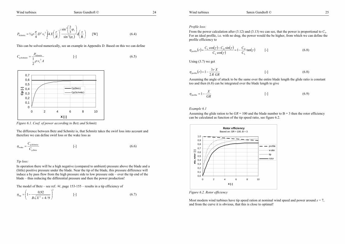
RrXvDP [W] (6.4)

This can be solved numerically, see an example in Appendix D. Based on this we can define

Av

PC

31

SchmitzSchmitzp,

21 ρ

= [-] (6.5)

00,10,20,30,40,50,60,7

0 2 4 6 8 10

X [-]

Cp

[-] Cp(Betz)

Cp(Schmitz)

Figure 6.1. Coef. of power according to Betz and Schmitz The difference between Betz and Schmitz is, that Schmitz takes the swirl loss into account and therefore we can define swirl loss or the wake loss as

Betzp,

Schmitzp,wake C

C=η [-] (6.6)

Tip loss: In operation there will be a high negative (compared to ambient) pressure above the blade and a (little) positive pressure under the blade. Near the tip of the blade, this pressure difference will induce a by pass flow from the high pressure side to low pressure side – over the tip end of the blade – thus reducing the differential pressure and then the power production! The model of Betz – see ref. /4/, page 153-155 – results in a tip efficiency of

2

2tip9/4

92,01 ⎟⎟⎠

⎞⎜⎜⎝

⎛

+−=

XBη [-] (6.7)


Profile loss: From the power calculation after (3.12) and (3.13) we can see, that the power is proportional to Cx. For an ideal profile, i.e. with no drag, the power would the be higher, from which we can define the profile efficiency to

( ) ( ) ( )( ) ( )γγ

γγη tan1cos

sincos

L

D

L

DLprofile C

CC

CCr −=−

= [-] (6.8)

Using (3.7) we get

( )GRRXrr

231profile −=η [-] (6.8)

Assuming the angle of attack to be the same over the entire blade length the glide ratio is constant too and then (6.8) can be integrated over the blade length to give

GRX

−= 1profileη [-] (6.9)

Example 6.1 Assuming the glide ration to be GR = 100 and the blade number to B = 3 then the rotor efficiency can be calculated as function of the tip speed ratio, see figure 6.2.

Rotor efficiencyBased on: GR = 100; B = 3

0,00,10,2

0,30,40,50,60,7

0,80,91,0

0 2 4 6 8 10

X [-]

eta_

roto

r [-

]

prof ile

w ake

tip

rotor

Figure 6.2. Rotor efficiency Most modern wind turbines have tip speed ration at nominal wind speed and power around x = 7, and from the curve it is obvious, that this is close to optimal!


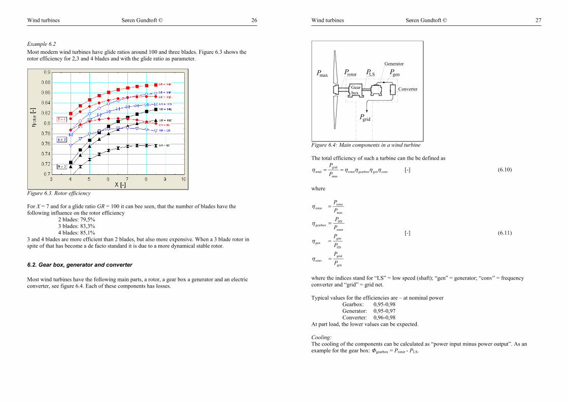
Example 6.2 Most modern wind turbines have glide ratios around 100 and three blades. Figure 6.3 shows the rotor efficiency for 2,3 and 4 blades and with the glide ratio as parameter.

Figure 6.3. Rotor efficiency For X = 7 and for a glide ratio GR = 100 it can bee seen, that the number of blades have the following influence on the rotor efficiency 2 blades: 79,5% 3 blades: 83,3% 4 blades: 85,1% 3 and 4 blades are more efficient than 2 blades, but also more expensive. When a 3 blade rotor in spite of that has become a de facto standard it is due to a more dynamical stable rotor.

6.2. Gear box, generator and converter Most wind turbines have the following main parts, a rotor, a gear box a generator and an electric converter, see figure 6.4. Each of these components has losses.


Pmax rotorP LSP genP

gridP

Gear box

Generator

Converter

Figure 6.4: Main components in a wind turbine The total efficiency of such a turbine can the be defined as

convgengearboxrotormax

gridtotal ηηηηη ==

PP

[-] (6.10)

where

gen

gridconv

HS

gengen

rotor

HSgearbox

max

rotorrotor

PPPPPPPP

=

=

=

=

η

η

η

η

[-] (6.11)

where the indices stand for “LS” = low speed (shaft); “gen” = generator; “conv” = frequency converter and “grid” = grid net. Typical values for the efficiencies are – at nominal power Gearbox: 0,95-0,98 Generator: 0,95-0,97 Converter: 0,96-0,98 At part load, the lower values can be expected. Cooling: The cooling of the components can be calculated as “power input minus power output”. As an example for the gear box: Φgearbox = Protor - PLS.


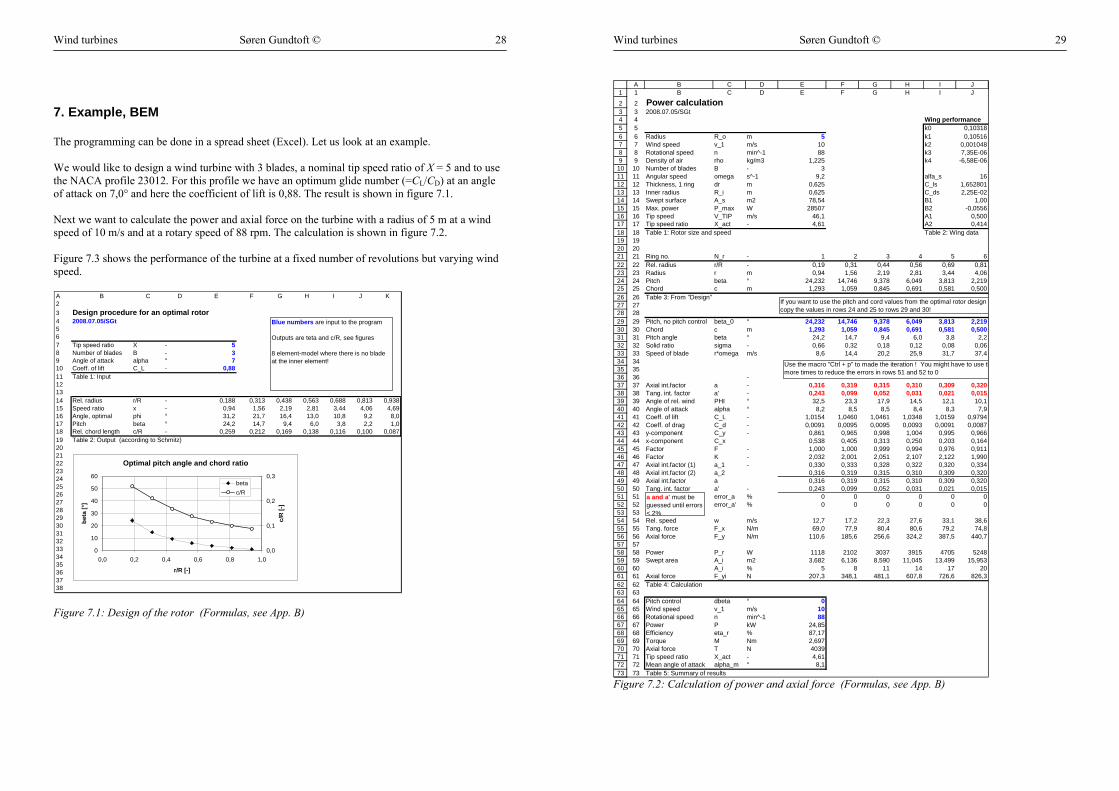
7. Example, BEM The programming can be done in a spread sheet (Excel). Let us look at an example. We would like to design a wind turbine with 3 blades, a nominal tip speed ratio of X = 5 and to use the NACA profile 23012. For this profile we have an optimum glide number (=CL/CD) at an angle of attack on 7,0° and here the coefficient of lift is 0,88. The result is shown in figure 7.1. Next we want to calculate the power and axial force on the turbine with a radius of 5 m at a wind speed of 10 m/s and at a rotary speed of 88 rpm. The calculation is shown in figure 7.2. Figure 7.3 shows the performance of the turbine at a fixed number of revolutions but varying wind speed. A B C D E F G H I J K23 Design procedure for an optimal rotor4 2008.07.05/SGt567 Tip speed ratio X - 58 Number of blades B - 39 Angle of attack alpha ° 710 Coeff. of lift C_L - 0,8811 Table 1: Input121314 Rel. radius r/R - 0,188 0,313 0,438 0,563 0,688 0,813 0,93815 Speed ratio x - 0,94 1,56 2,19 2,81 3,44 4,06 4,6916 Angle, optimal phi ° 31,2 21,7 16,4 13,0 10,8 9,2 8,017 Pitch beta ° 24,2 14,7 9,4 6,0 3,8 2,2 1,018 Rel. chord length c/R - 0,259 0,212 0,169 0,138 0,116 0,100 0,08719 Table 2: Output (according to Schmitz)20212223242526272829303132333435363738

Optimal pitch angle and chord ratio

0

10

20

30

40

50

60

0,0 0,2 0,4 0,6 0,8 1,0

r/R [-]

beta

[°]

0,0

0,1

0,2

0,3

c/R

[-]

betac/R

Blue numbers are input to the program

Outputs are teta and c/R, see figures

8 element-model where there is no blade at the inner element!

Figure 7.1: Design of the rotor (Formulas, see App. B)


1

23456789

10111213141516171819202122232425262728293031323334353637383940414243444546474849505152535455565758596061626364656667686970717273

A B C D E F G H I J1 B C D E F G H I J

2 Power calculation3 2008.07.05/SGt4 Wing performance5 k0 0,103186 Radius R_o m 5 k1 0,105167 Wind speed v_1 m/s 10 k2 0,0010488 Rotational speed n min^-1 88 k3 7,35E-069 Density of air rho kg/m3 1,225 k4 -6,58E-0610 Number of blades B - 311 Angular speed omega s^-1 9,2 alfa_s 1612 Thickness, 1 ring dr m 0,625 C_ls 1,65280113 Inner radius R_i m 0,625 C_ds 2,25E-0214 Swept surface A_s m2 78,54 B1 1,0015 Max. power P_max W 28507 B2 -0,055616 Tip speed V_TIP m/s 46,1 A1 0,50017 Tip speed ratio X_act - 4,61 A2 0,41418 Table 1: Rotor size and speed Table 2: Wing data192021 Ring no. N_r - 1 2 3 4 5 622 Rel. radius r/R - 0,19 0,31 0,44 0,56 0,69 0,8123 Radius r m 0,94 1,56 2,19 2,81 3,44 4,0624 Pitch beta ° 24,232 14,746 9,378 6,049 3,813 2,21925 Chord c m 1,293 1,059 0,845 0,691 0,581 0,50026 Table 3: From "Design"272829 Pitch, no pitch control beta_0 ° 24,232 14,746 9,378 6,049 3,813 2,21930 Chord c m 1,293 1,059 0,845 0,691 0,581 0,50031 Pitch angle beta ° 24,2 14,7 9,4 6,0 3,8 2,232 Solid ratio sigma - 0,66 0,32 0,18 0,12 0,08 0,0633 Speed of blade r*omega m/s 8,6 14,4 20,2 25,9 31,7 37,4343536 -37 Axial int.factor a - 0,316 0,319 0,315 0,310 0,309 0,32038 Tang. int. factor a' - 0,243 0,099 0,052 0,031 0,021 0,01539 Angle of rel. wind PHI ° 32,5 23,3 17,9 14,5 12,1 10,140 Angle of attack alpha ° 8,2 8,5 8,5 8,4 8,3 7,941 Coeff. of lift C_L - 1,0154 1,0460 1,0461 1,0348 1,0159 0,979442 Coeff. of drag C_d - 0,0091 0,0095 0,0095 0,0093 0,0091 0,008743 y-component C_y - 0,861 0,965 0,998 1,004 0,995 0,96644 x-component C_x 0,538 0,405 0,313 0,250 0,203 0,16445 Factor F - 1,000 1,000 0,999 0,994 0,976 0,91146 Factor K - 2,032 2,001 2,051 2,107 2,122 1,99047 Axial int.factor (1) a_1 - 0,330 0,333 0,328 0,322 0,320 0,33448 Axial int.factor (2) a_2 0,316 0,319 0,315 0,310 0,309 0,32049 Axial int.factor a 0,316 0,319 0,315 0,310 0,309 0,32050 Tang. int. factor a' - 0,243 0,099 0,052 0,031 0,021 0,01551 error_a % 0 0 0 0 0 052 error_a' % 0 0 0 0 0 05354 Rel. speed w m/s 12,7 17,2 22,3 27,6 33,1 38,655 Tang. force F_x N/m 69,0 77,9 80,4 80,6 79,2 74,856 Axial force F_y N/m 110,6 185,6 256,6 324,2 387,5 440,75758 Power P_r W 1118 2102 3037 3915 4705 524859 Swept area A_i m2 3,682 6,136 8,590 11,045 13,499 15,95360 A_i % 5 8 11 14 17 2061 Axial force F_yi N 207,3 348,1 481,1 607,8 726,6 826,362 Table 4: Calculation6364 Pitch control dbeta ° 065 Wind speed v_1 m/s 1066 Rotational speed n min^-1 8867 Power P kW 24,8568 Efficiency eta_r % 87,1769 Torque M Nm 2,69770 Axial force T N 403971 Tip speed ratio X_act - 4,6172 Mean angle of attack alpha_m ° 8,173 Table 5: Summary of results

a and a' must be guessed until errors < 2%

Use the macro "Ctrl + p" to made the iteration ! You might have to use thmore times to reduce the errors in rows 51 and 52 to 0

If you want to use the pitch and cord values from the optimal rotor design ycopy the values in rows 24 and 25 to rows 29 and 30!

Figure 7.2: Calculation of power and axial force (Formulas, see App. B)


0

10

20

30

40

50

60

70

80

90

0 5 10 15 20 25 30

Wind speed [m/s]

Pow

er [k

W]

0

10

20

30

40

5060

70

80

90

100

0 2 4 6 8 10

Tip speed ratio [-]

Effic

ienc

y [%

]

Figure 7.3: Power as function of wind speed (left) and efficiency as function of tip speed ratio (right)

8. Distribution of wind and annual energy production

Weibull distribution The wind is distributed close to the Weibull distribution curve. For practical purposes one can calculate the probability for the wind being in the interval vi < v < vi+1

( )⎟⎟

⎠

⎞

⎜⎜

⎝

⎛

⎥⎥⎦

⎤

⎢⎢⎣

⎡⎟⎠⎞

⎜⎝⎛−−

⎟⎟

⎠

⎞

⎜⎜

⎝

⎛

⎥⎥⎦

⎤

⎢⎢⎣

⎡⎟⎠⎞

⎜⎝⎛−=<< +

+

kk

Av

Av

vvvp 1ii1ii expexp [-] (8.1)

where A and k are found for a given site on the basis of measurements.

Annual production If the power for the turbine at a given wind speed is P(u), the annual production can be calculated as

( ) ( ){ }∑ +<<⋅= m1iiann h8766 vPvvvpE [J] (8.2) where vm is the mean value of vi and vi+1 i.e. vm = ( vi + vi+1)/2.

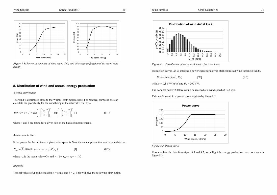
Example Typical values of A and k could be A = 8 m/s and k = 2. This will give the following distribution


Distribution of wind A=8 & k = 2

0,000,020,040,060,080,100,120,14

0,5

2,5

4,5

6,5

8,5

10,5

12,5

14,5

16,5

18,5

20,5

22,5

24,5

v_m [m/s]

p(v(

i)<v<

v(i+

1))

Figure 8.1: Distribution of the natural wind – for ∆v = 1 m/s Production curve: Let us imagine a power curve for a given stall controlled wind turbine given by

P(v) = min ( kP v3, PN ) [W] (8.3) with kP = 0,1 kW/(m/s)3 and PN = 200 kW. The nominal power 200 kW would be reached at a wind speed of 12,6 m/s. This would result in a power curve as given by figure 8.2.

Power curve

0

50

100

150

200

250

0 5 10 15 20 25 30

Wind speed, v [m/s]

P(v

) [kW

]

Figure 8.2. Power curve If we combine the data from figure 8.1 and 8.2, we will get the energy production curve as shown in figure 8.3.


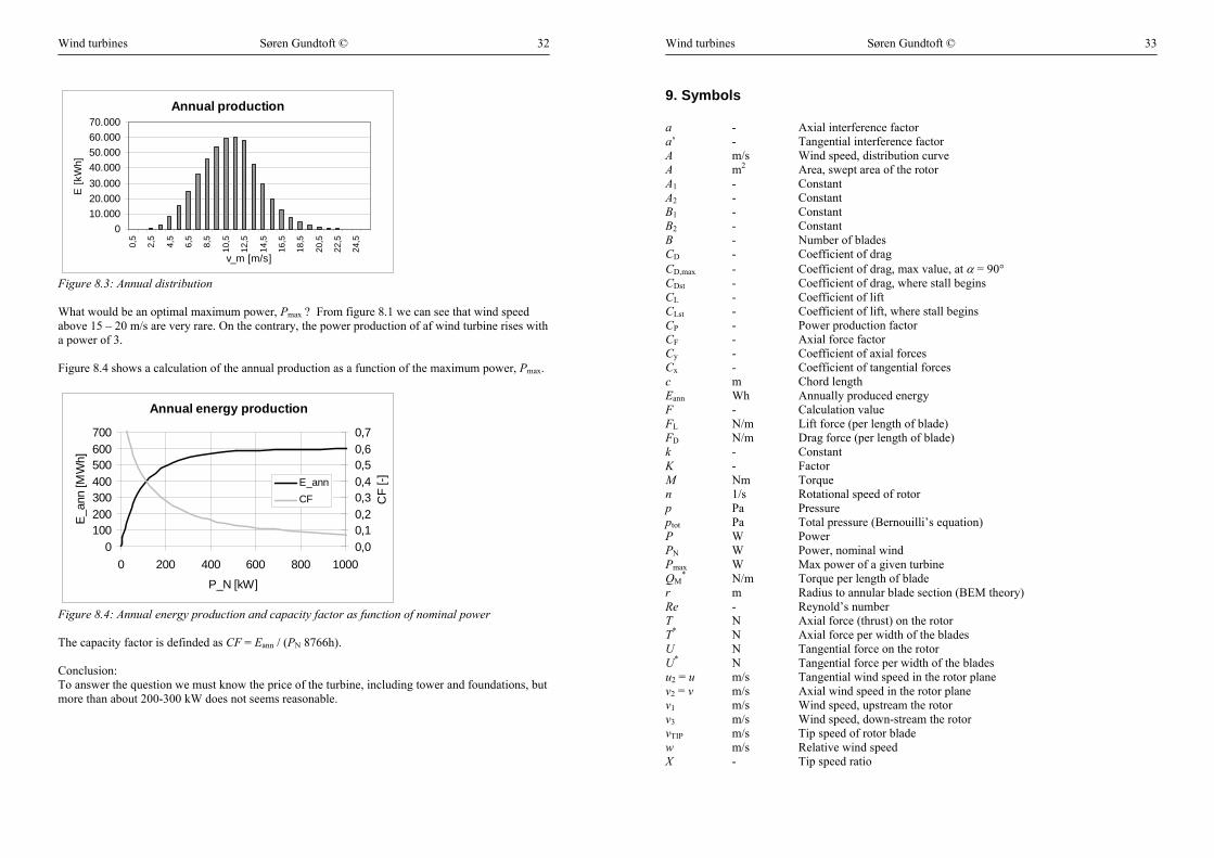
Annual production

010.00020.00030.00040.00050.00060.00070.000

0,5

2,5

4,5

6,5

8,5

10,5

12,5

14,5

16,5

18,5

20,5

22,5

24,5

v_m [m/s]

E [k

Wh]

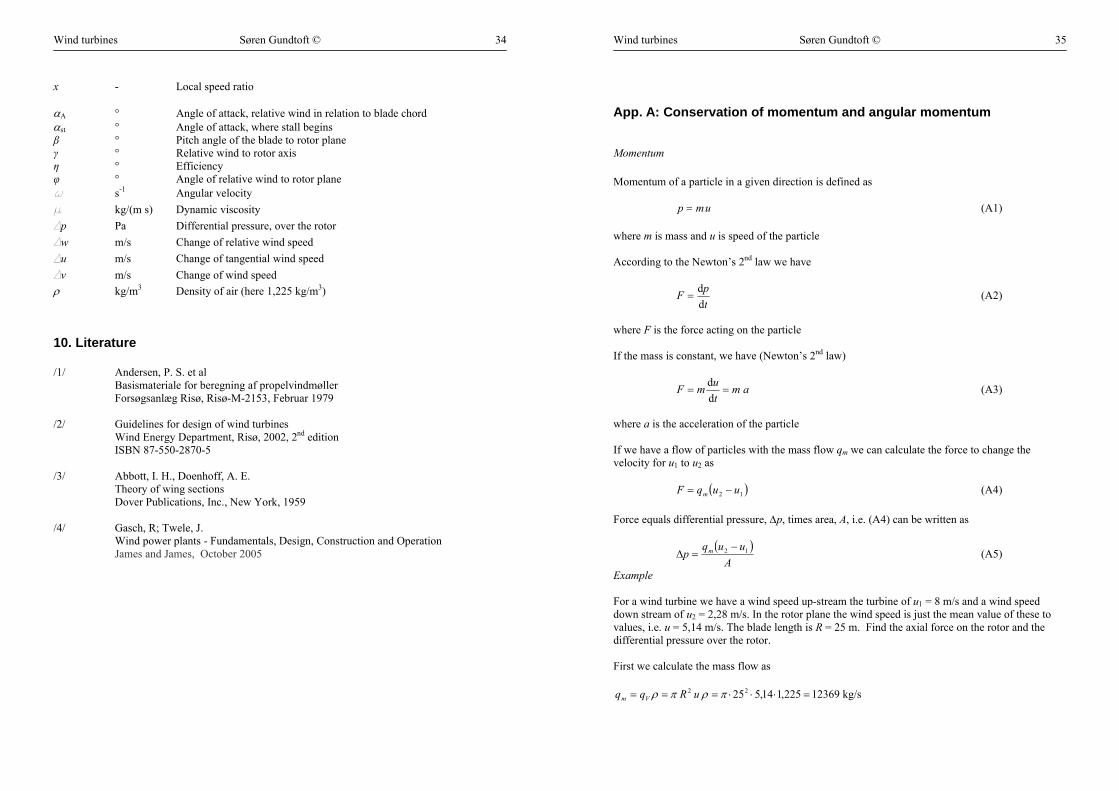
Figure 8.3: Annual distribution What would be an optimal maximum power, Pmax ? From figure 8.1 we can see that wind speed above 15 – 20 m/s are very rare. On the contrary, the power production of af wind turbine rises with a power of 3. Figure 8.4 shows a calculation of the annual production as a function of the maximum power, Pmax.

Annual energy production

0100200300400500600700

0 200 400 600 800 1000

P_N [kW]

E_a

nn [M

Wh]

0,00,10,20,30,40,50,60,7

CF

[-]E_annCF

Figure 8.4: Annual energy production and capacity factor as function of nominal power The capacity factor is definded as CF = Eann / (PN 8766h). Conclusion: To answer the question we must know the price of the turbine, including tower and foundations, but more than about 200-300 kW does not seems reasonable.


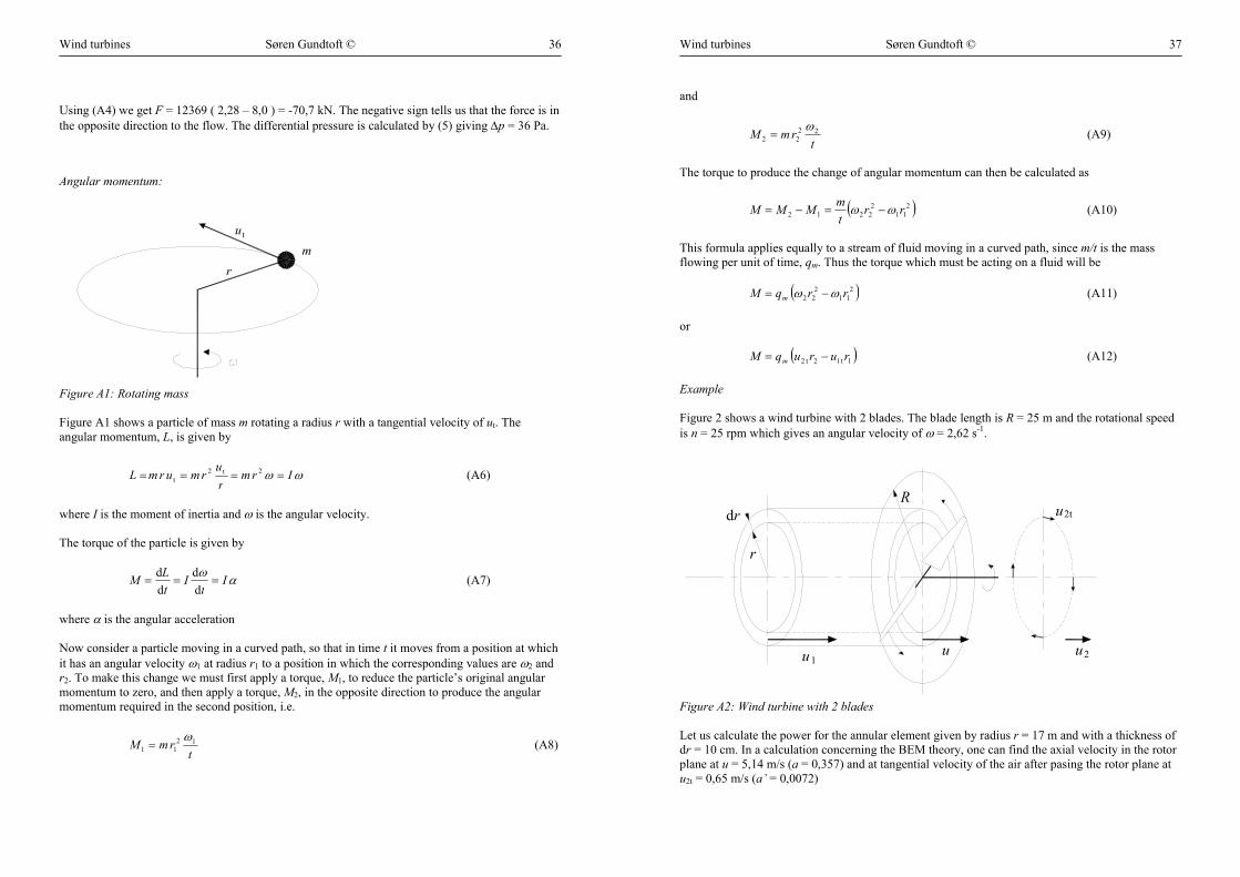
9. Symbols a - Axial interference factor a’ - Tangential interference factor A m/s Wind speed, distribution curve A m2 Area, swept area of the rotor A1 - Constant A2 - Constant B1 - Constant B2 - Constant B - Number of blades CD - Coefficient of drag CD,max - Coefficient of drag, max value, at α = 90° CDst - Coefficient of drag, where stall begins CL - Coefficient of lift CLst - Coefficient of lift, where stall begins CP - Power production factor CF - Axial force factor Cy - Coefficient of axial forces Cx - Coefficient of tangential forces c m Chord length Eann Wh Annually produced energy F - Calculation value FL N/m Lift force (per length of blade) FD N/m Drag force (per length of blade) k - Constant K - Factor M Nm Torque n 1/s Rotational speed of rotor p Pa Pressure ptot Pa Total pressure (Bernouilli’s equation) P W Power PN W Power, nominal wind Pmax W Max power of a given turbine QM

* N/m Torque per length of blade r m Radius to annular blade section (BEM theory) Re - Reynold’s number T N Axial force (thrust) on the rotor T* N Axial force per width of the blades U N Tangential force on the rotor U* N Tangential force per width of the blades u2 = u m/s Tangential wind speed in the rotor plane v2 = v m/s Axial wind speed in the rotor plane v1 m/s Wind speed, upstream the rotor v3 m/s Wind speed, down-stream the rotor vTIP m/s Tip speed of rotor blade w m/s Relative wind speed X - Tip speed ratio


x - Local speed ratio αA ° Angle of attack, relative wind in relation to blade chord αst ° Angle of attack, where stall begins β ° Pitch angle of the blade to rotor plane γ ° Relative wind to rotor axis η ° Efficiency φ ° Angle of relative wind to rotor plane ω s-1 Angular velocity µ kg/(m s) Dynamic viscosity ∆p Pa Differential pressure, over the rotor ∆w m/s Change of relative wind speed ∆u m/s Change of tangential wind speed ∆v m/s Change of wind speed ρ kg/m3 Density of air (here 1,225 kg/m3)

10. Literature /1/ Andersen, P. S. et al Basismateriale for beregning af propelvindmøller Forsøgsanlæg Risø, Risø-M-2153, Februar 1979 /2/ Guidelines for design of wind turbines Wind Energy Department, Risø, 2002, 2nd edition ISBN 87-550-2870-5 /3/ Abbott, I. H., Doenhoff, A. E. Theory of wing sections Dover Publications, Inc., New York, 1959 /4/ Gasch, R; Twele, J. Wind power plants - Fundamentals, Design, Construction and Operation

James and James, October 2005


App. A: Conservation of momentum and angular momentum

Momentum Momentum of a particle in a given direction is defined as

ump = (A1) where m is mass and u is speed of the particle According to the Newton’s 2nd law we have

tpF

dd

= (A2)

where F is the force acting on the particle If the mass is constant, we have (Newton’s 2nd law)

amtumF ==

dd (A3)

where a is the acceleration of the particle If we have a flow of particles with the mass flow qm we can calculate the force to change the velocity for u1 to u2 as

( )12 uuqF m −= (A4) Force equals differential pressure, ∆p, times area, A, i.e. (A4) can be written as

( )A

uuqp m 12 −=∆ (A5)

Example For a wind turbine we have a wind speed up-stream the turbine of u1 = 8 m/s and a wind speed down stream of u2 = 2,28 m/s. In the rotor plane the wind speed is just the mean value of these to values, i.e. u = 5,14 m/s. The blade length is R = 25 m. Find the axial force on the rotor and the differential pressure over the rotor. First we calculate the mass flow as

kg/s12369225,114,52522 =⋅⋅⋅=== πρπρ uRqq Vm


Using (A4) we get F = 12369 ( 2,28 – 8,0 ) = -70,7 kN. The negative sign tells us that the force is in the opposite direction to the flow. The differential pressure is calculated by (5) giving ∆p = 36 Pa.

Angular momentum:

rm

u t

Figure A1: Rotating mass Figure A1 shows a particle of mass m rotating a radius r with a tangential velocity of ut. The angular momentum, L, is given by

ωω Irmru

rmurmL ==== 2t2t (A6)

where I is the moment of inertia and ω is the angular velocity. The torque of the particle is given by

αω It

ItLM ===

dd

dd (A7)

where α is the angular acceleration Now consider a particle moving in a curved path, so that in time t it moves from a position at which it has an angular velocity ω1 at radius r1 to a position in which the corresponding values are ω2 and r2. To make this change we must first apply a torque, M1, to reduce the particle’s original angular momentum to zero, and then apply a torque, M2, in the opposite direction to produce the angular momentum required in the second position, i.e.

trmM 1211ω

= (A8)


and

trmM 22

22ω

= (A9)

The torque to produce the change of angular momentum can then be calculated as

( )211

22212 rr

tmMMM ωω −=−= (A10)

This formula applies equally to a stream of fluid moving in a curved path, since m/t is the mass flowing per unit of time, qm. Thus the torque which must be acting on a fluid will be

( )211

222 rrqM m ωω −= (A11)

or

( )1t12t2 ruruqM m −= (A12) Example Figure 2 shows a wind turbine with 2 blades. The blade length is R = 25 m and the rotational speed is n = 25 rpm which gives an angular velocity of ω = 2,62 s-1.

R

r

dr

uu

u2t

1u2

Figure A2: Wind turbine with 2 blades Let us calculate the power for the annular element given by radius r = 17 m and with a thickness of dr = 10 cm. In a calculation concerning the BEM theory, one can find the axial velocity in the rotor plane at u = 5,14 m/s (a = 0,357) and at tangential velocity of the air after pasing the rotor plane at u2t = 0,65 m/s (a’ = 0,0072)


The mass flow through the annular element is

( )( ) ( )( ) kg/s0,68225,114,5171,017d 2222 =⋅⋅−+=−+== πρπρ urrrqq Vm In formula (A12) we have u1t = 0 because there is no rotation of the air before the rotor plane and u2t = 0,65 m/s and r1 = r2 = r = 17 m. The torque can be calculated at

( ) Nm755000,1765,00,68 =⋅−⋅=M The power can be calculated at P = M ω = 1,98 kW


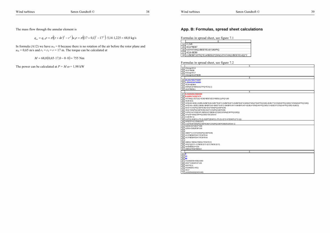
App. B: Formulas, spread sheet calculations Formulas in spread sheet, see figure 7.1

1415161718

E=1,5/8=E14*$E$7=2/3*ATAN(1/$E$7/E14)*180/PI()=E16-$E$9=1/$E$8*16*PI()*E14/$E$10*(SIN(1/3*ATAN(1/$E$7/E14)))^2

Formulas in spread sheet, see figure 7.2

22232425

E=Design!E14=E22*$E$6=Design!E17=Design!E18*$E$6

2930313233

E24,23174017732971,29343334743683=E29+$E$64=MIN(E30*$E$10/(2*PI()*E23);1)=E23*$E$11

37383940414243444546474849505152535455565758596061

E0,3164645126694690,24291710357473=ATAN((1-E37)/(1+E38)*$E$7/(E23*$E$11))/PI()*180=E39-E31=IF(E40<$J$11;$J$5+$J$6*E40+$J$7*E40^2+$J$8*E40^3+$J$9*E40^4;$J$16*SIN(2*E40*PI()/180)+$J$17*(COS(E40*PI()/180))^2/SIN(E40*PI()/180))=IF(E40<=$J$11;$K$5+$K$6*E40+$K$7*E40^2+$K$8*E40^3+$K$9*E40^4;$J$14*SIN(E40*PI()/180)^2+$J$15*COS(E40*PI()/180)+$J$13)=E41*COS(PI()/180*E39)+E42*SIN(PI()/180*E39)=E41*SIN(PI()/180*E39)-E42*COS(PI()/180*E39)=2/PI()*ACOS(EXP(-$E$10/2*($E$6-E23)/E23/SIN(E39*PI()/180)))=4*E45*SIN(E39*PI()/180)^2/E32/E43=1/(E46+1)=1/2*(2+E46*(1-2*0,2)-SQRT((E46*(1-2*0,2)+2)^2+4*(E46*0,2^2-1)))=IF(E37>0,2;E48;E47)=1/(4*E45*SIN(PI()/180*E39)*COS(PI()/180*E39)/E32/E44-1)=(E49-E37)/E37*100=(E50-E38)/E38*100

=$E$7*(1-E37)/SIN(PI()/180*E39)=0,5*$E$9*E54^2*E30*E44=0,5*$E$9*E54^2*E30*E43

=$E$11*$E$10*$E$12*E55*E23=PI()*(((E21+1)*$E$13)^2-(E21*$E$13)^2)=E59/$E$14*100=$E$10*E56*$E$13

646566676869707172

E01088=SUM(E58:K58)/1000=E67*1000/E15*100=E67/E11=SUM(E61:K61)=E17=AVERAGE(E40:K40)


The iteration to find a and a’ in row 37 and row 38 (see example on figure 10) can be quite tedious. The job can be done automatically by the following macro. Run the macro by typing “Ctrl + p”. Sub Makro1() ' ' Makro1 Makro ' Makro indspillet 13-10-03 af Søren Gundtoft ' ' Genvejstast:Ctrl+p ' Range("E50:K50").Select Application.CutCopyMode = False Selection.Copy Range("E38").Select Selection.PasteSpecial Paste:=xlValues, Operation:=xlNone, SkipBlanks:= _ False, Transpose:=False Range("E49:K49").Select Application.CutCopyMode = False Selection.Copy Range("E37").Select Selection.PasteSpecial Paste:=xlValues, Operation:=xlNone, SkipBlanks:= _ False, Transpose:=False Range("E50:K50").Select Application.CutCopyMode = False Selection.Copy Range("E38").Select Selection.PasteSpecial Paste:=xlValues, Operation:=xlNone, SkipBlanks:= _ False, Transpose:=False Range("E49:K49").Select Application.CutCopyMode = False Selection.Copy Range("E37").Select Selection.PasteSpecial Paste:=xlValues, Operation:=xlNone, SkipBlanks:= _ False, Transpose:=False Range("E50:K50").Select Application.CutCopyMode = False Selection.Copy Range("E38").Select Selection.PasteSpecial Paste:=xlValues, Operation:=xlNone, SkipBlanks:= _ False, Transpose:=False Range("E49:K49").Select Application.CutCopyMode = False Selection.Copy Range("E37").Select Selection.PasteSpecial Paste:=xlValues, Operation:=xlNone, SkipBlanks:= _ False, Transpose:=False Range("E50:K50").Select Application.CutCopyMode = False Selection.Copy Range("E38").Select Selection.PasteSpecial Paste:=xlValues, Operation:=xlNone, SkipBlanks:= _ False, Transpose:=False Range("E49:K49").Select Application.CutCopyMode = False Selection.Copy Range("E37").Select Selection.PasteSpecial Paste:=xlValues, Operation:=xlNone, SkipBlanks:= _ False, Transpose:=False End Sub


App. C: Formulas, EES-programme "BEM-model 2008.07.07/SGt" PROCEDURE C_lift_and_drag(alpha:C_lift;C_drag) "#####################################################################" "This procedure calculates the coefficient of lift and drag for the NACA23012 profile" alpha_s=16 C_dmax=1 "lift and drag at stall" C_lift_s=1,0318E-01+1,0516E-01*alpha_s+1,0483E-03*alpha_s^2+7,3487E-06*alpha_s^3-6,5827E-06*alpha_s^4 C_drag_s=6,0387E-03-3,6282E-04*alpha_s+5,4269E-05*alpha_s^2+6,5341E-06*alpha_s^3-2,8045E-07*alpha_s^4 "Some constants" B1=C_dmax B2=1/COS(alpha_s)*(C_drag_s-C_dmax*SIN(alpha_s)^2) A1=B1/2 A2=(C_lift_s-C_dmax*SIN(alpha_s)*COS(alpha_s))*(SIN(alpha_s)/(COS(alpha_s))^2) IF alpha<alpha_s THEN C_lift=1,0318E-01+1,0516E-01*alpha+1,0483E-03*alpha^2+7,3487E-06*alpha^3-6,5827E-06*alpha^4 C_drag=6,0387E-03-3,6282E-04*alpha+5,4269E-05*alpha^2+6,5341E-06*alpha^3-2,8045E-07*alpha^4 ELSE C_lift = A1*sin(2*alpha)+A2*(cos(alpha))^2/sin(alpha) C_drag = B1*(sin(alpha))^2 + B2*cos(alpha) + C_drag_s ENDIF END PROCEDURE interference_factors(V_0;omega;B;R;ri;c;betai: a_axial;a_tangential;C_x;C_y) "#####################################################################" "Initialize" a_axial=0,3 a_tangential=0,000001 REPEAT "Reset old iteration values" a_axial_old=a_axial a_tangential_old=a_tangential "Calculate angle of attack and solidity" phi=arctan(((1-a_axial)/(1+a_tangential))*(V_0/(ri*omega))) {Determine rel. angle of attack, [rad]} alpha=phi-betai {Determine actual angle of attack correcting for pitch, [°] } sigma=(c*B)/(2*pi*ri) {Determine solidity, [-] } CALL C_lift_and_drag(alpha:C_l;C_d) C_y=C_l*COS(phi)+C_d*SIN(phi) C_x=C_l*SIN(phi)-C_d*COS(phi) "Perform Prandtl tiploss correction" g=(B/2)*(R-ri)/(ri*sin(phi)) expmg=exp(-g) F=(2/pi)*(arccos(expmg)*pi/180) K=4*F*SIN(phi)^2/sigma/C_y a_1=1/(4*F*SIN(phi)^2/sigma/C_y+1) hj=max((K*(1-2*0,2)+2)^2+4*(K*0,2^2-1);0,000001) a_2=1/2*(2+K*(1-2*0,2)-SQRT(hj)) IF a_axial_old>0,2 THEN a_axialx=a_2 ELSE a_axialx=a_1 ENDIF a_tangentialx=1/(4*F*SIN(phi)*COS(phi)/sigma/C_x-1) "Underdamping" underdamping_factor=0,5 a_axial=a_axial_old+underdamping_factor*(a_axialx-a_axial_old)


a_tangential=a_tangential_old+0,5*(a_tangentialx-a_tangential_old) error_a=sqrt(( (a_axial-a_axial_old)/a_axial_old*100 )^2) error_t=sqrt(((a_tangential-a_tangential_old)/a_tangential_old*100)^2) epsilon=0,01 UNTIL((error_a<epsilon) AND (error_t<epsilon)) END "Procedure" "#####################################################################" " M A I N P R O G R A M " "#####################################################################" R=5 "[m] Radius of rotor" B=3 "[-] Number of blades" V_0=10 "[m/s] Wind speed" n=88/60 "[rps] Rotor speed" rho_a=1,225 "[kg/m3] Density of air" beta_p=0 "[°] Pitch angle" n_elements=8 "[-] Number of ring elements" omega = 2*pi*n "[s^-1] Angular speed" "The model devides the blande in 8 ring element, with no air foil in the inner element" DUPLICATE i=1;7 r_div_R[i]=(i+0,5)/8 END "chord and pitch angle" c_div_R[1]=0,2889 : beta_0[1]=23,92 c_div_R[2]=0,2249 : beta_0[2]=14,98 c_div_R[3]=0,1787 : beta_0[3]=9,96 c_div_R[4]=0,1474 : beta_0[4]=6,76 c_div_R[5]=0,1252 : beta_0[5]=4,56 c_div_R[6]=0,1088 : beta_0[6]=2,96 c_div_R[7]=0,0961 : beta_0[7]=1,74 DUPLICATE i=1;7 beta[i]= beta_0[i]+beta_p END "BEM" DUPLICATE i=1;7 r[i]=r_div_R[i]*R c[i]=c_div_R[i]*R CALL interference_factors(V_0;omega;B;R;r[i];c[i];beta[i]: a_axial[i];a_tangential[i];C_x[i];C_y[i]) w_rel[i]=sqrt((omega*r[i]*(1+a_tangential[i]))^2+((1-a_axial[i])*V_0)^2) F_x[i]=0,5*rho_a*w_rel[i]^2*c[i]*C_x[i] F_y[i]=0,5*rho_a*w_rel[i]^2*c[i]*C_y[i] P[i]=R/8*B*omega*F_x[i]*r[i] Fa[i]=B*R/8*F_y[i] END P_rotor=SUM(P[i];i=1;7)/1000 F_rotor=SUM(Fa[i];i=1;7) P_r_max=16/27*pi*R^2*1/2*rho_a*V_0^3/1000 eta_r=P_rotor/P_r_max*100


App. D: Formulas, EES-programme, to solve the integral in (6.4) "Efficiency of a wind turbine rotor" "08.07.2008/SGt" FUNCTION fCp_schmitz(X) "This function calculates the Cp-wake factor according to Schmitz's theory 09.07.2008/SG" i_max = 1000 dRR = 1/i_max i = -1 x_sum = 0 REPEAT i = i+1 RR = i/i_max IF (RR=0) THEN phi = 90 ELSE phi = arctan(1/(X*RR)) ENDIF xx = 4*X*RR^2*(sin(2/3*phi))^3/(sin(phi)^2)*dRR x_sum = x_sum + xx UNTIL (i=i_max) fCp_schmitz = x_sum END "========= Main =========" GR = 100 "[-] - Glide ratio = C_L/C_D" B = 3 "[-] - Number of blades" X=7 "[-] - Tip speed ratio" Cp_Betz = 16/27 Cp_Schmitz = fCp_Schmitz(X) eta_profile = 1-X/GR eta_tip = (1-0,92/(B*sqrt(X^2+4/9)))^2 eta_tip_s = 1 - 1,84/B/X Cp_Real = Cp_Schmitz*eta_profile*eta_tip eta_wake = Cp_Schmitz/Cp_Betz eta_rotor = eta_wake*eta_profile*eta_tip

vel. diagrams

Documents