arX

iv:2

111.

0896

6v2

[ph

ysic

s.fl

u-dy

n] 7

Jan

202

2

Commun. Theor. Phys.

Nonequilibrium effects of reactive flow based

on gas kinetic theory∗

Xianli Su, and Chuandong Lin†

Sino-French Institute of Nuclear Engineering and Technology, Sun Yat-Sen University, Zhuhai 519082, China.

(Received XXXX; revised manuscript received XXXX)

How to accurately probe chemically reactive flows with essential thermodynamic nonequilibrium

effects is an open issue. Via the Chapman-Enskog analysis, the local nonequilibrium particle velocity

distribution function is derived from the gas kinetic theory. It is demonstrated theoretically and

numerically that the distribution function depends on the physical quantities and derivatives, and

is independent of the chemical reactions directly. Based on the simulation results of the discrete

Boltzmann model, the departure between equilibrium and nonequilibrium distribution functions is

obtained and analyzed around the detonation wave. Besides, it has been verified for the first time

that the kinetic moments calculated by summations of the discrete distribution functions are close to

those calculated by integrals of their original forms.

Keywords: Discrete Boltzmann method, Reactive flow, Detonation, Nonequilibrium

effect.

∗This work is supported by the National Natural Science Foundation of China (NSFC) under Grant No.

51806116.†Chuandong Lin, E-mail: linchd3@mail.sysu.edu.cn

Chemical reactive flow is a complex physicochemical phenomenon which is ubiquitous in

aerospace, energy and power fields, etc.[1, 2]

. It exhibits multiscale characteristics in tempo-

ral and spatial scales, incorporates various hydrodynamic and thermodynamic nonequilibrium

effects[3]. The nonequilibrium effects exert significant influences on fluid systems especially in

extremely complex environments[3], such as the spacecraft reentry into the atmosphere

[4], multi-

component reactive flow in porous media[5], fuel cells

[6, 7], phase separation

[8], hydrodynamic

instability[9], and detonation

[10]. At present, how to accurately probe, predict and analyze

chemical reactive flows with essential nonequilibrium effects is still an open issue.

Actually, there are various classes of methodologies to retain the information of velocity

distribution functions for fluid systems. For example, on the basis of the distribution function,

Nagnibeda et al. established the kinetic theory of transport processes and discussed the features

of complex system strongly deviating from the thermal and chemical equilibrium[3]. Besides, on

the microscopic level, the distribution function can be obtained by using the direct simulation

Monte Carlo[11, 12]

, or molecular dynamics[13, 14]

. As a kinetic mesoscopic methodology, the

discrete Boltzmann method (DBM) is a special discretization of the Boltzmann equation in

particle velocity space, and has been successfully developed to recover and probe the velocity

distribution functions of nonequilibrium physical systems[10, 15, 16, 17, 18, 19]

.

In fact, the DBM is based on statistical physics and regarded as a variant of the traditional

lattice Boltzmann method (LBM)[20, 21, 22, 23, 24]

. Compare to standard LBMs, the DBM can

address more issues, in particular to simulate the compressible fluid systems with significant

nonequilibrium effects[15, 19, 25, 26, 27, 28, 29, 30]

. At present, there are two means to recover the

velocity distribution functions. One relies on the analysis of the detailed nonequilibrium phys-

ical quantities to obtain the main features of the velocity distribution function in a qualitative

way[10, 15, 16, 18]

. The other is to recover the detailed velocity distribution function by means of

macroscopic quantities and their spatio derivatives quantitatively, which can be derived by using

the Chapman-Enskog expansion[17, 19]

. The two methods are consistent with each other[19]

.

In the rest of this paper, we firstly derive the nonequilibrium velocity distribution function

of reactive fluid based on the Boltzmann equation. Secondly, we give a brief introduction

2

of the DBM for compressible reactive flows. Thirdly, the DBM is utilized to investigate the

kinetic moments of the velocity distribution function around the detonation wave. Finally, the

nonequilibrium and equilibrium distribution functions as well as their differences are obtained

and analyzed.

Now, let us introduce the popular Bhatanger-Gross-Krook (BGK) Boltzmann equation,

∂f

∂t+v ⋅ ∇f =

1τ (f − f

eq) + R, (1)

where τ denotes the relaxation time, t the time, f the velocity distribution function. The

equilibrium distribution function[18]

is

feq= n( 1

2πT)D/2( 1

2πIT)1/2 exp [− ∣v − u∣2

2T−

η2

2IT] , (2)

where D = 2 denotes the dimensional translational degree of freedom, I stands for extra degrees

of freedom due to vibration and/or rotation, and η represents the corresponding vibrational

and/or rotational energies. Here n is the particle number density, u the hydrodynamic velocity,

T the temperature, m = 1 the particle mass, and ρ = nm the mass density.

On the right-hand side of Eq. (1), R is the chemical term describing the change rate of the

distribution function due to chemical reactions, i.e.,

R =

df

dt

»»»»»»»R. (3)

To derive the explicit expression of the chemical term, the following qualifications are assumed[26]

:

tmr < tcr < tsys, where tmr, tcr and tsys represent the time scale of molecular relaxation, the time

scale of chemical reaction and the characteristic time scale of the system, respectively. Under

the condition tmr < tcr, Eq. (3) can be approximated by

R ≈

dfeq

dt

»»»»»»»»R =

∂feq

∂ρ

∂ρ

∂t

»»»»»»»R +∂f

eq

∂u

∂u

∂t

»»»»»»»R +∂f

eq

∂T

∂T

∂t

»»»»»»»R, (4)

as feq

is the function of ρ, u, and T , respectively. Furthermore, the assumption tcr < tsys

leads to the following conclusion: the chemical reaction results in the change of temperature

directly, as the density and flow velocity remain unchanged during the rapid reaction process.

Consequently, Eq. (4) can be reduced to

R =

∂feq

∂T

∂T

∂t

»»»»»»»R. (5)

3

Substituting Eq. (2) into Eq. (5) gives

R = feq× [−D + 1

2T+∣v − u∣22T 2

+η2

2IT 2] 2Qλ

′

D + I, (6)

where Q indicates the chemical heat release per unit mass of fuel, λ′is the change rate of the

mass fraction of chemical product. Additionally, a two-step reaction scheme is employed to

mimic the essential dynamics of a chain-branching reaction of detonation in this paper[31]

.

Via the Chapman-Enskog analysis, we derive the first-order approximation formula of the

velocity distribution function of reacting flows through the macroscopic quantities and their

spatial and temporal derivatives,

f = feq− τ [∂f eq

∂ρ(∂ρ∂t

+ vα∂ρ

∂rα)

+∂f

eq

∂T(∂T∂t

+ vα∂T

∂rα) + ∂f

eq

∂uβ

(∂uβ

∂t+ vα

∂uβ

∂rα)]

+ τ (∂f eq

∂T

∂T

∂t

»»»»»»»R) , (7)

in terms of∂f

eq

∂ρ= f

eq×1ρ, (8)

∂feq

∂T= f

eq× [−D + 1

2T+∣v − u∣22T 2

+η2

2IT 2] , (9)

and∂f

eq

∂uβ

= feq×(vβ − uβ)

T. (10)

Note that the change rate of temperature consists of two parts, i.e.,

∂T

∂t=∂T

∂t

»»»»»»»R −2T

D + I

∂uα

∂rα− uα

∂T

∂rα, (11)

on the right-hand side of which the first term describes the part caused by the heat release of

chemical reactions,∂T

∂t

»»»»»»»R=2Qλ

′

D + I, (12)

and the other two terms reflect the parts due to the spatial gradients of velocity and tempera-

ture.

4

Therefore, Eq. (7) can be simplified as

f = feq− τ [∂f eq

∂ρ(∂ρ∂t

+ vα∂ρ

∂rα)

+∂f

eq

∂T(− 2T

D + I

∂uα

∂rα− uα

∂T

∂rα+ vα

∂T

∂rα)

+∂f

eq

∂uβ

(∂uβ

∂t+ vα

∂uβ

∂rα)] , (13)

with∂ρ

∂t= −ρ

∂uα

∂rα− uα

∂ρ

∂rα. (14)

It can be found from Eqs. (11), (12) and (14) that the temporal derivatives can be expressed

by the spatial derivatives. Those formulas are obtained from the Chapman-Enskog expansion.

In fact, there are two ways to calculate the simulation results of∂ρ

∂tor ∂T

∂t. One method is to

calculate the temporal change rate directly. For example,

∂ρ

∂t=

ρt+∆t

− ρt−∆t

2∆t.

The other method is to use Eqs. (11) or (14) where the spatial derivatives can be computed by

the finite difference scheme. The results given by the two methods are similar to each other.

Moreover, it can be inferred from Eq. (13) that the chemical reaction term is eliminated,

so it has no contribution to the velocity distribution function directly. This is due to the

aforementioned assumption that the chemical time scale is longer than the molecular relaxation

time. The case where the chemical time scale is close to or less than the molecular relaxation

time is not considered in this work.

In this work, the BGK DBM is used to mimic and measure the nonequilibrium reactive

flows[18]

. The discretization of the model in particle velocity space takes the form

∂fi

∂t+ viα

∂fi

∂rα=1τ (fi − f

eq

i ) +Ri, (15)

where fi and feq

irepresent the discrete distribution function and its equilibrium counterpart,

respectively. vi denotes the discrete velocity with i = 1, 2, 3, ⋯, N , and N = 16 is the total

number of discrete velocities. Here a two-dimensional sixteen-velocity model is employed, see

Fig. 1.

5

14 13

1

15 16

2

3

4

56

78

9

10

11

12

Figure 1: Sketch for the discrete velocity model.

Physically, the DBM is approximately equivalent to a continuous fluid model plus a coarse-

grained model for discrete effects. Meanwhile, the DBM is roughly equivalent to a hydrody-

namic model plus a coarse-grained model of thermodynamic nonequilibrium behaviors. For

the sake of recovering the NS equations in the hydrodynamic limit, the discrete equilibrium

distribution functions feq

iare required to satisfy the following relationship,

∬ feqΨdvdη = ∑

ifeq

i Ψi, (16)

with the particle velocities Ψ = 1, v, (v ⋅ v + η2), vv, (v ⋅ v + η

2)v, vvv, (v ⋅ v + η2)vv, and

the corresponding discrete velocities, Ψi = 1, vi, (vi ⋅ vi + η2i ), vivi, (vi ⋅ vi + η

2i )vi, vivivi,

(vi ⋅ vi + η2i )vivi.

Furthermore, one merit of the DBM is to capture nonequilibrium information described by

the following (but not limited to) high-order kinetic moments

M2 = ∑i

fivivi, (17)

Meq

2 = ∑i

feq

i vivi, (18)

M3,1 = ∑i

fi (vi ⋅ vi + η2i )vi, (19)

Meq

3,1 = ∑i

feq

i (vi ⋅ vi + η2i )vi, (20)

6

M3 = ∑i

fivivivi, (21)

Meq

3 = ∑i

feq

i vivivi, (22)

M4,2 = ∑i

fi (vi ⋅ vi + η2i )vivi, (23)

Meq

4,2 = ∑i

feq

i (vi ⋅ vi + η2i )vivi, (24)

∆2 = M2 −Meq

2 , (25)

∆3,1 = M3,1 −Meq

3,1, (26)

∆3 = M3 −Meq

3 , (27)

∆4,2 = M4,2 −Meq

4,2, (28)

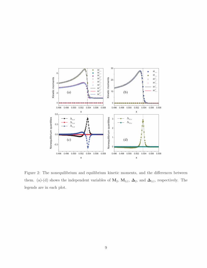
where the M2, M3,1, M3 and M4,2 are the kinetic moments of the distribution functions,

Meq

2 , Meq

3,1, Meq

3 and Meq

4,2 denote the corresponding equilibrium counterparts, ∆2, ∆3,1, ∆3

and ∆4,2 are the differences between them. Here, ∆2 represents the viscous stress tensor and

nonorganized momentum flux, ∆3,1 and ∆3 are relevant to the nonorganized energy fluxes.

∆4,2 is related to the flux of nonorganized energy flux.

To verify the consistency of theoretical and numerical results of the nonequilibrium manifes-

tations of reactive flows, firstly, we simulate a reaction process in a uniform resting system. The

specific-heat ratio is γ = 5/3, the chemical heat release Q = 1, the space step ∆x = ∆y = 5×10−5,

the time step ∆t = 2 × 10−6, and the discrete velocities (va, vb, vc, vd, ηa, ηb, ηc, ηd) = (3.7,

3.2, 1.4, 1.4, 2.4, 0, 0, 0), respectively. In order to possess a high computational efficiency, only

one mesh grid (Nx × Ny = 1 × 1) is used, and the periodic boundary condition is adopted in

each direction, because the physical field is uniformly distributed. It is found that all simulated

nonequilibrium physical quantities (including ∆2, ∆3,1, ∆3, and ∆4,2) remain zero during the

evolution. Therefore, in the process of the chemical reaction, the deviation of velocity distri-

bution function f from its equilibrium counterpart feq

is zero, i.e f = feq. Besides, all physical

gradients are zero in the simulation process due to the uniform distribution of physical quan-

tities. Consequently, it is numerically verified that the chemical reaction does not contribute

7

to the nonequilibrium effects directly.∗

This result is consistent with the aforementioned the-

ory that the distribution function depends on the physical quantities and derivatives, and is

independent of chemical reactions directly, see Eq. (13).

For the purpose of further validation, the one-dimensional (1-D) steady detonation is sim-

ulated. The initial configuration, obtained from the Hugoniot relation, takes the form

⎧⎪⎪⎪⎨⎪⎪⎪⎩(ρ, ux, uy, T, ξ, λ)L = (1.38549, 0.70711, 0, 2.01882, 1, 1) ,(ρ, ux, uy, T, ξ, λ)R = (1, 0, 0, 1, 0, 0) ,

where the subscript L indicates 0 ≤ x ≤ 0.00555, and R indicates 0.00555 < x ≤ 0.555. The Mach

number is 1.96. To ensure the resolution is high enough, the grid is chosen asNx×Ny = 11100×1,

other parameters are the same as before. Furthermore, the inflow and/or outflow boundary

conditions are employed in the x direction, and the periodic boundary condition is adopted in

the y direction.

Figure 2 displays the kinetic moments of velocity distribution function (M2,xx, M2,xy, M2,yy,

M3,1,x, M3,1,y), the equilibrium counterparts (Meq

2,xx, Meq

2,xy, Meq

2,yy, Meq

3,1,x, Meq

3,1,y), and the

nonequilibrium quantities (∆2,xx, ∆2,xy, ∆2,yy, ∆3,1,x,∆3,1,y) around the detonation front. Here

∆2,xx represents twice the nonorganized energy in the x degree of freedom, and ∆2,yy twice the

nonorganized energy in the y degree of freedom. ∆3,1,x and ∆3,1,y denote twice the nonorganized

energy fluxes in the x and y directions, respectively. The dashed line is located at the position

x = 0.50375.

In Fig. 2 (a), the solid squares, circles and triangles stand for the DBM results of kinetic

moments of distribution function M2,xx,M2,xy, and M2,yy, respectively. The hollow squares, cir-

cles and triangles represent the DBM results of the kinetic moments of equilibrium distribution

function Meq

2,xx, Meq

2,xy, and Meq

2,yy, respectively. And the solid lines indicate the corresponding

analytic solutions, Meq

2,xx = ρ (T + u2x), Meq

2,xy = ρuxuy, and Meq

2,yy = ρ (T + u2y), respectively. With

the detonation wave propagating from left to right, M2,xx, Meq

2,xx, M2,yy, Meq

2,yy first increase due

∗It should be mentioned that the chemical reaction may change the physical gradients which make an impact

on the nonequilibrium effects. In other words, the chemical reaction plays an indirect role in nonequilibrium

effect of the reactive flows.

8

(a)

(d)(c)

(b)

2 ,xx

eq

M

2 ,xxM

2 ,xyM

2 , yyM

2 ,xy

eq

M

2 , yy

eq

M

2 ,xx

eq

M

2 ,xy

eq

M

2 , yy

eq

M

3,1,xM

3,1, yM

3,1,x

eq

M

3,1,x

eq

M

3,1, y

eq

M

3,1, y

eq

M

2,xx

2,xy

2,yy

3,1,x

3,1,y

Figure 2: The nonequilibrium and equilibrium kinetic moments, and the differences between

them. (a)-(d) shows the independent variables of M2, M3,1, ∆2, and ∆3,1, respectively. The

legends are in each plot.

9

to the compressible effect, then decrease owing to the rarefaction effect, and form a peak around

the detonation front. Meanwhile, M2,xy and Meq

2,xy remain zero, because the detonation wave

propagates forwards in the x direction. In addition, as for the equilibrium kinetic moments

(Meq

2,xx, Meq

2,xy, and Meq

2,yy), the DBM results are in good agreement with the analytical solutions.

In Fig. 2 (b), the solid squares and circles represent M3,1,x and M3,1,y, respectively. The hal-

low symbols denote the equilibrium counterparts Meq

3,1,x, and Meq

3,1,y. And the solid lines indicate

the analytic solutions Meq

3,1,x = ρux [(D + I + 2)T + u2] and M

eq

3,1,y = ρuy [(D + I + 2)T + u2].

Similarly, M3,1,x and Meq

3,1,x ascend rapidly and then decline slowly due to the compressible

and rarefaction effects, respectively. M3,1,y and Meq

3,1,y are still zero in the one-dimensional

simulation.

In Fig. 2 (c), as the detonation wave travels from left to right, ∆2,xx expressed by the solid

line with squares first increases, then decreases, and increases afterwards, so it forms a high

positive peak and a negative trough. Actually, Fig. 2 (c) is consistent with Fig 2 (a) where

M2,xx first greater than Meq

2,xx and then less than Meq

2,xx as the detonation wave travels forwards.

Physically, ∆2,xx stands for twice the nonorganized energy in the x direction, its positive peak

and the negative trough correspond to the compression and rarefaction effects, respectively.

The solid line with triangles denotes twice the nonorganized energy in the y direction ∆2,yy,

which first decreases to form a negative trough and then increases to form a low positive peak.

This trend is also consistent with the results of M2,yy and Meq

2,yy in the Fig. 2 (a). Additionally,

∆2,xy = M2,xy −Meq

2,xy = 0 in Fig. 2 (c) is in line with M2,xy = Meq

2,xy = 0 in Fig. 2 (a).

In Fig. 2 (d), ∆3,1,x and ∆3,1,y denote twice the nonorganized energy fluxes in the x and

y directions, respectively. ∆3,1,x and ∆3,1,y are the differences between the kinetic moment

M3,1,x,M3,1,y and their equilibrium counterparts Meq

3,1,x,Meq

3,1,y, respectively. Obviously, ∆3,1,x

forms a positive peak and then a low negative trough. Because the M3,1,x first greater and then

less than Meq

3,1,x. Besides, the M3,1,y and Meq

3,1,y are zero, which causes ∆3,1,y = M3,1,y −Meq

3,1,y to

be zero as well.

Next, let us verify that the kinetic moments calculated by the summations of the discrete

distribution functions are close to those calculated by integrals of their original forms at the

location x = 0.50375. The kinetic moments calculated by the summations of the discrete

10

distribution functions are (∆2,xx, ∆2,xy, ∆2,yy, ∆3,1,x, ∆3,1,y) = (0.48449, 0, −0.35844, 2.89123,

0), while the results of the corresponding integration counterparts are (∆2,xx, ∆2,xy, ∆2,yy,

∆3,1,x, ∆3,1,y) = (0.56488, 0, −0.27255, 2.80181, 0). The relative errors are (17%, 0%, 24%, 3%,

0%), which is roughly satisfactory. For the first time, this test demonstrates the accuracy of

the nonequilibrium manifestations measured by the DBM, and validates the consistence of the

DBM with its theoretical basis.

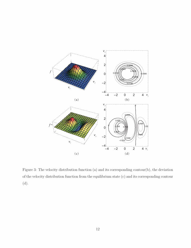
To further perform a quantitative study of the nonequilibrium state around the detonation

wave, Fig. 3 (a) displays the velocity distribution function at the peak of ∆2,xx, which is on

the vertical dashed line in Fig. 2. It is clear that the velocity distribution function has a peak

in the two-dimensional velocity space. Actually, due to the nonequilibrium effects, the veloc-

ity distribution function deviates from its local equilibrium counterpart, i.e., the Maxwellian

velocity distribution function.

In order to have an intuitive study of the local velocity distribution function, Fig. 3 (b)

shows its contours in the velocity space, which is in line with Fig. 3 (a). Clearly, the peak is

asymmetric in the vx direction and symmetric in the vy direction. The contour lines are close

to each other near the peak (especially on the left side), and becomes sparse away from the

peak (especially on the right side). That is to say, the gradient is sharp near the peak (on the

left side in especial), and smooth far from the peak (on the left side in especial).

To have a deep understanding of the deviation of the velocity distribution function from the

equilibrium state, Fig. 3 (c) depicts the difference between the nonequilibrium and equilibrium

distribution functions in the two-dimensional velocity space. It is obvious that there are both

positive and negative deviations around the detonation wave. Along the vx direction, a high

positive peak first appears, then decreases to form a valley, and then increases to a low positive

peak.

As can be seen in Fig. 3 (d), the deviation is symmetric about vy = 0, and asymmetric

about vx = ux. The contour plot consists of three segments along the vx direction. The leftmost

segment is in the region of the first peak, where the contour lines are approximately elliptical.

The middle part is in the low valley area that seems like a “moon” shape. And the rightmost

one is in the low peak area, which likes a cobblestone. The contour lines between the high peak

11

（a）

（d）（c）

（b）

f

neqf

yv

xv

xv

yv

xv

xv

yv

yv

Figure 3: The velocity distribution function (a) and its corresponding contour(b), the deviation

of the velocity distribution function from the equilibrium state (c) and its corresponding contour

(d).

12

(a)

(d)

(b)

(c)

xf v

xf v

yf v

yf v

eqyf veq

xf v

neqxf v neq

yf v

xu

xu

xv

xv

yv

yv

Figure 4: One-dimensional nonequilibrium and equilibrium distribution functions in the vx (a)

and vy (b) directions, and the differences between them in the vx (c) and vy (d) directions.

and the valley are closer to each other than those between the valley and low peak, because

the gradients between the leftmost and middle parts are sharp than those between the middle

and rightmost regions.

Finally, let us investigate the one-dimensional distribution functions and the corresponding

deviations from the equilibrium states. Figures 4 (a) and (b) depict the velocity distribution

functions in the vx and vy directions, respectively. The solid lines represent the velocity dis-

tribution functions f (vx) = ∬ fdvydη and f (vy) = ∬ fdvxdη, the dashed curves express the

equilibrium counterparts feq(vx) = ∬ f

eqdvydη and f

eq(vy) = ∬ feqdvxdη, respectively. Figures

4 (c) and (d) show fneq(vx) = f (vx) − f

eq(vx) and fneq(vy) = f (vy) − f

eq(vy) which indicate the

departures of distribution functions from the equilibrium state in the vx and vy directions,

respectively. The following points can be obtained.

(I) In Figs. 4 (a) - (b), there is a peak for each curve of f (vx), f eq(vx), f (vy), and feq(vy). In

Figs. 4 (c) - (d), there are two peaks and a trough for fneq(vx), while a peak and two troughs

for fneq(vy). Along the vx direction, f

neq(vx) forms a positive peak firstly, then decreases to

13

form a valley, and then increases to a second positive peak. Because f (vx) is first greater thanfeq(vx), then less than f

eq(vx), and finally greater than feq(vx) again. Similarly, the relation

f (vy) > feq(vy) or f (vy) < f

eq(vy) in Fig. 4 (b) leads to the results fneq(vy) > 0 or f

neq(vy) < 0 in

Fig. 4 (d).

(II) f (vx) and fneq(vx) are asymmetric about the vertical dashed line located at vx = ux,

while feq(vx) is symmetric. Physically, as the detonation evolves, the compressible effect plays

a significant role in the front of the detonation wave, and the internal energy in the x degree of

freedom increases faster than in other degrees of freedom, and there exists nonorganized heat

flux in the x direction.

(III) In Figs. 4 (b) and (d), each curve of f (vy), f eq(vy) and fneq(vy) has a positive peak

which is symmetric about vy = 0. On the left and right parts of fneq(vy) are two identical troughs

that are symmetrically distributed in Fig. 4 (b). Because the periodic boundary condition is

imposed on the y direction, the equilibrium and nonequilibrium velocity distributions for vy > 0

and vy < 0 are symmetrical.

(IV) The nonequilibrium manifestations in Figs. 2 (a)-(d) are consistent with the deviations

of distribution functions in Figs. 4 (a)-(d). Specifically, the trend of fneq(vx) indicates that f (vx)

is “fatter” and “lower” than feq(vx), which means the nonorganized momentum flux ∆2,xx > 0.

The trend of fneq(vy) means that f (vy) is “thinner” and “higher” than f

eq(vy), which indicates

∆2,yy < 0. Meanwhile, the portion f (vx > ux) is “fatter” than the part f (vx < ux), whichis named “positive skewness” and indicates ∆3,1,x > 0. And the symmetry of f

neq(vy) means

∆3,1,y = 0.

In conclusion, via the Chapman-Enskog expansion, the velocity distribution function of

compressible reactive flows is expressed by using the macroscopic quantities and their spa-

tial derivatives. The equilibrium and nonequilibrium distribution functions in one- and two-

dimensional velocity spaces are recovered quantitatively from the physical quantities of the

DBM, which is an accurate and efficient gas kinetic method. The departure between the equi-

librium and nonequilibrium distribution functions is in line with the nonequilibrium quantities

measured by the DBM. Moreover, it is for the first time to verify that the kinetic moments

measured by summations of the distribution function resemble those assessed by integrals of

14

the original forms, which consists with the theoretical basis of the DBM. In addition, under the

condition that the chemical time scale is longer than the molecular relaxation time, it is nu-

merically and theoretically demonstrated that the chemical reaction imposes no direct impact

on the thermodynamic nonequilibrium effects.

15

References

[1] Elaine S Oran and Jay P Boris. Numerical simulation of reactive flow. Cambridge universitypress, 2005.

[2] C. K. Law. Combustion physics. Cambridge University Press, Cambridge, 2006.

[3] E. Nagnibeda and E. Kustova. Non-equilibrium reacting gas flows: kinetic theory of transportand relaxation processes. Springer, Berlin, 2009.

[4] Frank J Regan. Dynamics of atmospheric re-entry. Aiaa, 1993.

[5] Ruben Juanes. Nonequilibrium effects in models of three-phase flow in porous media. Advancesin Water Resources, 31(4):661–673, 2008.

[6] Li Chen, Mengyi Wang, Qinjun Kang, and Wenquan Tao. Pore scale study of multiphase mul-ticomponent reactive transport during co2 dissolution trapping. Advances in water resources,116:208–218, 2018.

[7] Hao Wu, Peter Berg, and Xianguo Li. Steady and unsteady 3d non-isothermal modeling of pemfuel cells with the effect of non-equilibrium phase transfer. Applied Energy, 87(9):2778–2784,2010.

[8] Yanbiao Gan, Aiguo Xu, Guangcai Zhang, and Sauro Succi. Discrete boltzmann modelingof multiphase flows: Hydrodynamic and thermodynamic non-equilibrium effects. Soft Matter,11(26):5336–5345, 2015.

[9] Huilin Lai, Aiguo Xu, Guangcai Zhang, Yanbiao Gan, Yangjun Ying, and Sauro Succi. Nonequi-librium thermohydrodynamic effects on the rayleigh-taylor instability in compressible flows. Phys-ical Review E, 94(2):023106, 2016.

[10] Chuandong Lin and Kai H Luo. Mesoscopic simulation of nonequilibrium detonation with discreteboltzmann method. Combustion and Flame, 198:356–362, 2018.

[11] Carlo Cercignani, Aldo Frezzotti, and Patrick Grosfils. The structure of an infinitely strong shockwave. Physics of fluids, 11(9):2757–2764, 1999.

[12] Ahmad Shoja-Sani, Ehsan Roohi, and Stefan Stefanov. Homogeneous relaxation and shock waveproblems: Assessment of the simplified and generalized bernoulli trial collision schemes. Physicsof Fluids, 33(3):032004, 2021.

[13] VV Zhakhovskii, K Nishihara, and SI Anisimov. Shock wave structure in dense gases. Journalof Experimental and Theoretical Physics Letters, 66(2):99–105, 1997.

[14] Awadhesh Kumar Dubey, Anna Bodrova, Sanjay Puri, and Nikolai Brilliantov. Velocity distri-bution function and effective restitution coefficient for a granular gas of viscoelastic particles.Physical Review E, 87(6):062202, 2013.

[15] Chuandong Lin, Aiguo Xu, Guangcai Zhang, and Yingjun Li. Polar coordinate lattice boltzmannkinetic modeling of detonation phenomena. Communications in Theoretical Physics, 62(5):737,2014.

[16] Chuandong Lin, Aiguo Xu, Guangcai Zhang, Yingjun Li, and Sauro Succi. Polar-coordinatelattice boltzmann modeling of compressible flows. Physical Review E, 89(1):013307, 2014.

16

[17] YuDong Zhang, Ai-Guo Xu, Guang-Cai Zhang, Zhi-Hua Chen, and Pei Wang. Discrete ellipsoidalstatistical bgk model and burnett equations. Frontiers of Physics, 13(3):1–13, 2018.

[18] Chuandong Lin and Kai H Luo. Discrete boltzmann modeling of unsteady reactive flows withnonequilibrium effects. Physical Review E, 99(1):012142, 2019.

[19] Chuandong Lin, Xianli Su, and Yudong Zhang. Hydrodynamic and thermodynamic nonequilib-rium effects around shock waves: Based on a discrete boltzmann method. Entropy, 22(12):1397,2020.

[20] Vasily Novozhilov and Conor Byrne. Lattice boltzmann modeling of thermal explosion in naturalconvection conditions. Numerical Heat Transfer, Part A: Applications, 63(11):824–839, 2013.

[21] Qing Li, Kai Hong Luo, QJ Kang, YL He, Q Chen, and Q Liu. Lattice boltzmann methods formultiphase flow and phase-change heat transfer. Progress in Energy and Combustion Science,52:62–105, 2016.

[22] Mostafa Ashna, Mohammad Hassan Rahimian, and Abbas Fakhari. Extended lattice boltzmannscheme for droplet combustion. Physical Review E, 95(5):053301, 2017.

[23] WW Yan, YF Yuan, JY Xiang, Y Wu, TY Zhang, SM Yin, and SY Guo. Construction oftriple-layered sandwich nanotubes of carbon@ mesoporous tio2 nanocrystalline@ carbon as high-performance anode materials for lithium-ion batteries. Electrochimica Acta, 312:119–127, 2019.

[24] Rui Du, Jincheng Wang, and Dongke Sun. Lattice-boltzmann simulations of the convection-diffusion equation with different reactive boundary conditions. Mathematics, 8(1):13, 2020.

[25] Bo Yan, Aiguo Xu, Guangcai Zhang, Yangjun Ying, and Hua Li. Lattice boltzmann model forcombustion and detonation. Frontiers of Physics, 8(1):94–110, 2013.

[26] Aiguo Xu, Chuandong Lin, Guangcai Zhang, and Yingjun Li. Multiple-relaxation-time latticeboltzmann kinetic model for combustion. Physical Review E, 91(4):043306, 2015.

[27] Chuandong Lin, Aiguo Xu, Guangcai Zhang, and Yingjun Li. Double-distribution-function dis-crete boltzmann model for combustion. Combustion and Flame, 164:137–151, 2016.

[28] Chuandong Lin, Kai Hong Luo, Linlin Fei, and Sauro Succi. A multi-component discrete boltz-mann model for nonequilibrium reactive flows. Scientific reports, 7(1):14580, 2017.

[29] Chuandong Lin and Kai Hong Luo. Mrt discrete boltzmann method for compressible exothermicreactive flows. Computers & Fluids, 166:176–183, 2018.

[30] Yanbiao Gan, Aiguo Xu, Guangcai Zhang, Yudong Zhang, and Sauro Succi. Discrete boltzmanntrans-scale modeling of high-speed compressible flows. Physical Review E, 97(5):053312, 2018.

[31] H. D. Ng, M. I. Radulescu, A. J. Higgins, N. Nikiforakis, and J. H. S. Lee. Numerical investigationof the instability for one-dimensional chapman-jouguet detonations with chain-branching kinetics.Combustion Theory and Modelling, 9(3):385–401, 2005.

17