1

Velocity Encoding and Flow Imaging

Michael Markl, Ph.D. University Hospital Freiburg, Dept. of Diagnostic Radiology, Medical Physics,

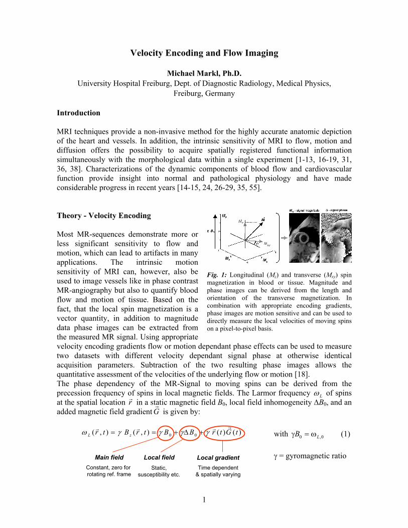
Freiburg, Germany Introduction MRI techniques provide a non-invasive method for the highly accurate anatomic depiction of the heart and vessels. In addition, the intrinsic sensitivity of MRI to flow, motion and diffusion offers the possibility to acquire spatially registered functional information simultaneously with the morphological data within a single experiment [1-13, 16-19, 31, 36, 38]. Characterizations of the dynamic components of blood flow and cardiovascular function provide insight into normal and pathological physiology and have made considerable progress in recent years [14-15, 24, 26-29, 35, 55]. Theory - Velocity Encoding Most MR-sequences demonstrate more or less significant sensitivity to flow and motion, which can lead to artifacts in many applications. The intrinsic motion sensitivity of MRI can, however, also be used to image vessels like in phase contrast MR-angiography but also to quantify blood flow and motion of tissue. Based on the fact, that the local spin magnetization is a vector quantity, in addition to magnitude data phase images can be extracted from the measured MR signal. Using appropriate velocity encoding gradients flow or motion dependant phase effects can be used to measure two datasets with different velocity dependant signal phase at otherwise identical acquisition parameters. Subtraction of the two resulting phase images allows the quantitative assessment of the velocities of the underlying flow or motion [18]. The phase dependency of the MR-Signal to moving spins can be derived from the precession frequency of spins in local magnetic fields. The Larmor frequency ωL of spins at the spatial location rr in a static magnetic field B0, local field inhomogeneity ΔB0, and an added magnetic field gradient

rG is given by:

0 0( , ) ( , ) ( ) ( )L zr t B r t B B r t G tω γ γ γ γ= = + Δ +rr r r

Main fieldConstant, zero for rotating ref. frame

Local fieldStatic,

susceptibility etc.

Local gradientTime dependent

& spatially varying

with 0,0 LB ω=γ (1) γ = gyromagnetic ratio

Fig. 1: Longitudinal (Mz) and transverse (Mxy) spin magnetization in blood or tissue. Magnitude and phase images can be derived from the length and orientation of the transverse magnetization. In combination with appropriate encoding gradients, phase images are motion sensitive and can be used to directly measure the local velocities of moving spins on a pixel-to-pixel basis.

2

After signal reception the acquired FID is demodulated with respect to the Larmor frequency 0,Lω in the static magnetic field B0. This corresponds to a transformation of the MR-Signal into a rotating reference frame such that the main field contribution to the signal frequency can be omitted for further calculations. Integration of equation (1) results in the phase of the precessing magnetization and thus the phase of the measured MR signal after an excitation pulse (at t0 ) at echo time TE:

∫∫ +−Δ==−TE

t

TE

tL dttrtGtTEBdttrtrTEr

00

.)()()(),(),(),( 000rrrrr γγωφφ (2)

which can be expanded in the following Taylor series:

,))((!

),()(),(),(

00

)(

0

0

)(000

0

∑ ∫

∑∞

=

∞

=

−+=

+−Δ+=

n

TE

t

nn

n

nn

dttttGn

r

TErtTEBtrTEr

rr

rrr

γφ

φγφφ

(3)

with r n( ) being the nth derivative of the time dependant spin position and nφ the corresponding nth order phase. Initial signal phase and field inhomogeneities result in an additional background phase 0φ . If the motion of the tissue under investigation does not change fast with respect to the temporal resolution of data acquisition the corresponding velocities can be approximated to be constant during data acquisition, i.e. echo time TE. Thus rr t( ) can be introduced as first order displacement ...)()( 00 +−+= ttvrtr rrr with a constant velocity ))(),(),(( 000 rvrvrvv zyx

rrrr= . Equation (3) then simplifies to

0 00 0

( , ) ( )d ( ) d ...TE TE

r TE r G t t v G t t tφ φ γ γ= + + +∫ ∫r rr r r

(4)

M0

static spinsM1

moving spins+ + …gradient

moments:

including an unknown background phase 0φ and zero and first order components which describe the influence of magnetic field gradients on phase components of static spins at 0r

r and moving spins with velocities vr , respectively. The integrals describing the contribution of the magnetic field gradients are also known as nth order gradient moments Mn such that the first gradient moment M1 determines the velocity induced signal phase for the constant velocity approximation. As a result, appropriate control of the first gradient moment can be used to specifically encode spin flow or motion. Velocity encoding is usually performed using bipolar gradients as depicted in figure 2, which, according to equation (4), result in zero M0 and thus do not lead to any phase encoding of stationary spins. Moving spins, however, will experience a linear velocity dependant phase change, which is proportional to the amplitude and timing of the gradient. According to equation (4) velocity induced phase shifts can be controlled by adjusting the

3

first gradient moment M1 by varying total bipolar gradient duration T and/or gradient strength G and are given by (simplified gradient design without ramps):

vTGvMv 211 )2/()( γγφ =−= (5)

However, background phase effects 0φ due to susceptibility of field inhomogeneity can not be refocused using bipolar gradients. To filter out such phase effects, two measurements with different first moments M1

(1) and M1(2) (e.g. inverted gradient

polarities) are thus necessary to isolate the velocity encoded phase shifts and encode flow or motion along a single direction. Subtraction of phase images from such two measurement results in phase differences Δφ which are directly proportional to the underlying velocities v and difference in first gradient moments ΔM = M1

(1) - M1(2).

Since Fourier image reconstruction resolves signal amplitudes and phases as a function of spatial locations, the encoded velocities can simply be derived from the data by dividing the pixel intensities in the calculated phase difference images by γΔM (figures 2 and 3). Note that only velocity components v along the direction of the bipolar gradient contribute to the phase of the MR-signal such that only a single velocity direction can be encoded with an individual measurement. As a result, at least four independent measurements with different arrangements of bipolar gradients have to be performed to gain velocity data with isotropic three-directional flow sensitivity. For the design of an actual phase contrast MR measurement, some prior knowledge of the order of the maximum velocities is required. For too high velocities, the velocity dependant phase shift can exceed +/-π and phase aliasing occurs. Velocity sensitivity ( 1Mvenc Δ= γπ ), is thus defined as the velocity that produces a phase shift Δφ of π radians and is determined by the difference of the first gradient moments used for velocity encoding. Consequently the highest velocity, which is expected, has to be used to define the velocity encoding (venc-factor) in order to avoid unintentional phase wrapping [45].

Fig. 2: Bipolar gradients with opposite polarity result in different first moments M1

(1) and M1(2). Phase

difference calculation eliminates the background phase and permits quantitative assessment flow or motion. Velocity aliasing occurs if the underlying motion exceeds venc.

Fig. 3: Top: Gradient echo pulse sequences for one-directional velocity encoding along the slice direction using bipolar gradients with opposite polarity. Bottom: Resulting through plane measurement of blood flow in the ascending (AAo) and descending (DAo) aorta. (Grey-scaled flow images = systolic blood flow velocities normal to the image plane. Note the enhanced velocity noise in regions of low SNR (lungs) in the magnitude images.

4

As for all MR imaging techniques, phase contrast velocity images suffer from noise that can lead to errors in the acquired velocities. It can be shown that the noise in the velocity encoded images, defined as the standard deviation σφ of the phase differences in a homogenous region with no flow or motion, is inversely related to the signal-to-noise ratio (SNR) in the corresponding magnitude images (σφ ~ 1/SNR) [36, 46]. Noise in the velocities derived from the phase difference data can therefore be estimated by

SNRvenc

v πσ 2

= . (6)

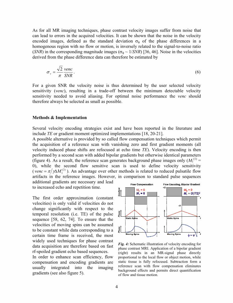
For a given SNR the velocity noise is thus determined by the user selected velocity sensitivity (venc), resulting in a trade-off between the minimum detectable velocity sensitivity needed to avoid aliasing. For optimal noise performance the venc should therefore always be selected as small as possible. Methods & Implementation Several velocity encoding strategies exist and have been reported in the literature and include TE or gradient moment optimized implementations [18, 20-21]. A possible alternative is provided by so called flow compensation techniques which permit the acquisition of a reference scan with vanishing zero and first gradient moments (all velocity induced phase shifts are refocused at echo time TE). Velocity encoding is then performed by a second scan with added bipolar gradients but otherwise identical parameters (figure 4). As a result, the reference scan generates background phase images only (M1

(1) = 0), while the second flow sensitive scan is used to define velocity sensitivity ( )2(

1Mvenc Δ= γπ ). An advantage over other methods is related to reduced pulsatile flow artifacts in the reference images. However, in comparison to standard pulse sequences additional gradients are necessary and lead to increased echo and repetition time. The first order approximation (constant velocities) is only valid if velocities do not change significantly with respect to the temporal resolution (i.e. TE) of the pulse sequence [58, 62, 74]. To ensure that the velocities of moving spins can be assumed to be constant while data corresponding to a certain time frame is received, the most widely used techniques for phase contrast data acquisition are therefore based on fast rf-spoiled gradient echo based sequences. In order to enhance scan efficiency, flow compensation and encoding gradients are usually integrated into the imaging gradients (see also figure 5).

Fig. 4: Schematic illustration of velocity encoding for phase contrast MRI. Application of a bipolar gradient (right) results in an MR-signal phase directly proportional to the local flow or object motion, while static tissue is fully refocused. Subtraction form a reference scan with flow compensation eliminates background effects and permits direct quantification of flow and tissue motion.

5

To synchronize phase contrast measurements with periodic tissue motion or pulsatile flow, data acquisition is typically gated to the cardiac cycle and time resolved (CINE) anatomical images are collected to depict the dynamics of tissue motion and blood flow during the cardiac cycle [19, 25-29, 33, 39, 50, 55, 70]. For phase contrast velocity mapping, bipolar gradients have to be introduced at appropriate positions and successive acquisitions have to be performed for reference scan and up to three motion sensitized acquisitions to derive one- to three-directional velocity fields from the data. To minimize artifacts in phase difference images related to subject motion, interleaved velocity encoding is often performed, for which the different flow encodes are kept as close together as possible in time (see figure 5). Flow Quantification & Visualization Visualization and quantification of blood flow and tissue motion using phase contrast (PC) MRI has been widely used in a number of applications. In addition to analyzing tissue motion such as left ventricular function [24, 35, 43, 51, 54, 66, 68], time-resolved 2D and 3D PC MRI have proven to be useful tools for the assessment of blood flow within the cardiovascular system [26-30, 32, 34, 44, 50, 52, 55, 56-57, 67, 70, 72]. Traditionally, MRI imaging of flow is accomplished using methods that resolve two spatial dimensions (2D) in individual slices. In combination with one-directional encoding of through plane velocities such methods are typically used for blood flow quantification in the heart and great vessels. Applications include the assessment of left ventricular performance (e.g. cardiac output), regurgitation volumes in case of valve insufficiency, or evaluation of flow acceleration in stenotic regions (e.g. aortic valve stenosis). Data analysis is typically based on semi-automatic segmentation of the vascular lumen of interest and calculation of time-resolved blood flow from mean flow velocities and vascular cross sectional area (figure 6).

Fig. 5: Example of ECG gated k-space segmented CINE phase contrast MRI for three-directional velocity encoding. For each k-space line a flow compensated reference scan and three motion sensitive scan (added bipolar gradients) are acquired in an interleaved manner. The temporal resolution and total scan time can be flexibly adjusted by the number of velocity sensitive acquisitions and k-space segments.

Fig. 6: Blood flow quantification in an axial slice above the aortic valve (bottom left) using through plane velocity encoding. Segmentation of vascular boundaries permits the calculation of mean, max and min blood flow velocities (lower right) to calculate average and peak flow rates. Visualization of systolic through plane flow profiles (top right) provide detailed insight into the temporal evolution of blood flow velocities.

6

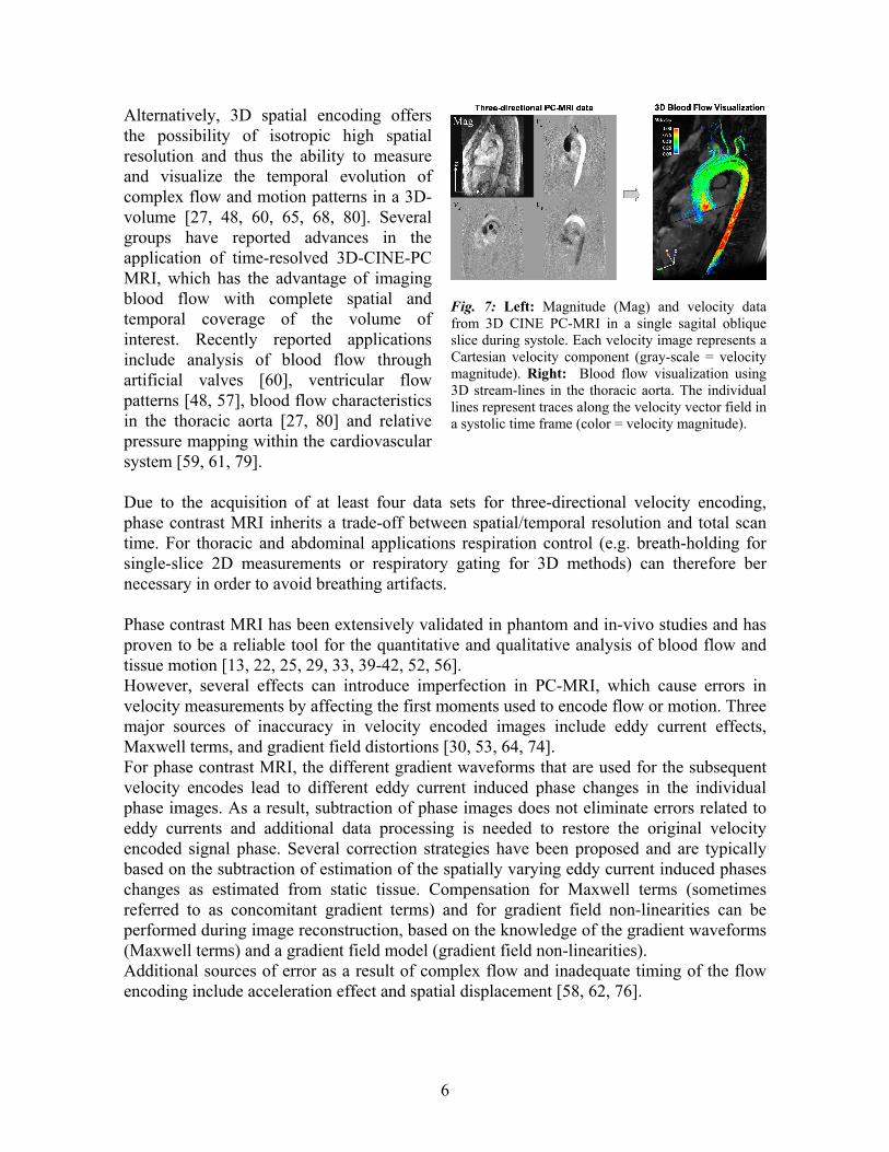
Alternatively, 3D spatial encoding offers the possibility of isotropic high spatial resolution and thus the ability to measure and visualize the temporal evolution of complex flow and motion patterns in a 3D-volume [27, 48, 60, 65, 68, 80]. Several groups have reported advances in the application of time-resolved 3D-CINE-PC MRI, which has the advantage of imaging blood flow with complete spatial and temporal coverage of the volume of interest. Recently reported applications include analysis of blood flow through artificial valves [60], ventricular flow patterns [48, 57], blood flow characteristics in the thoracic aorta [27, 80] and relative pressure mapping within the cardiovascular system [59, 61, 79]. Due to the acquisition of at least four data sets for three-directional velocity encoding, phase contrast MRI inherits a trade-off between spatial/temporal resolution and total scan time. For thoracic and abdominal applications respiration control (e.g. breath-holding for single-slice 2D measurements or respiratory gating for 3D methods) can therefore ber necessary in order to avoid breathing artifacts. Phase contrast MRI has been extensively validated in phantom and in-vivo studies and has proven to be a reliable tool for the quantitative and qualitative analysis of blood flow and tissue motion [13, 22, 25, 29, 33, 39-42, 52, 56]. However, several effects can introduce imperfection in PC-MRI, which cause errors in velocity measurements by affecting the first moments used to encode flow or motion. Three major sources of inaccuracy in velocity encoded images include eddy current effects, Maxwell terms, and gradient field distortions [30, 53, 64, 74]. For phase contrast MRI, the different gradient waveforms that are used for the subsequent velocity encodes lead to different eddy current induced phase changes in the individual phase images. As a result, subtraction of phase images does not eliminate errors related to eddy currents and additional data processing is needed to restore the original velocity encoded signal phase. Several correction strategies have been proposed and are typically based on the subtraction of estimation of the spatially varying eddy current induced phases changes as estimated from static tissue. Compensation for Maxwell terms (sometimes referred to as concomitant gradient terms) and for gradient field non-linearities can be performed during image reconstruction, based on the knowledge of the gradient waveforms (Maxwell terms) and a gradient field model (gradient field non-linearities). Additional sources of error as a result of complex flow and inadequate timing of the flow encoding include acceleration effect and spatial displacement [58, 62, 76].

Fig. 7: Left: Magnitude (Mag) and velocity data from 3D CINE PC-MRI in a single sagital oblique slice during systole. Each velocity image represents a Cartesian velocity component (gray-scale = velocity magnitude). Right: Blood flow visualization using 3D stream-lines in the thoracic aorta. The individual lines represent traces along the velocity vector field in a systolic time frame (color = velocity magnitude).

7

Summary and Discussion MRI provides a non-invasive method for the accurate anatomic characterization of the heart and great vessels in 3D. In addition, the intrinsic sensitivity of MRI to flow and motion offers the possibility to acquire spatially registered functional information simultaneously with the morphological data within a single phase contrast experiment. A disadvantage of phase contrast MRI is related to the need for multiple acquisitions for encoding a single velocity direction, resulting in long scan times. New methods based on the combination of phase contrast MRI and fast sampling strategies such as spiral or radial imaging or other imaging strategies such as balanced SSFP have been reported and are promising for further reduction in total scan time and/or increased spatial or temporal resolution [37, 63, 71]. In addition, the total acquisition time or temporal and spatial resolution associated with a specific MR technique may be further improved by using parallel imaging and/or partial k-space update methods (view sharing) [77, 78, 81]. MR velocity mapping has great potential to benefit from imaging at higher field strength. Recently reported results indicate a considerable gain in SNR [73], which is directly translated in reduced noise in the velocity encoded images and may also be used to increase spatial and/or temporal resolution. For the analysis and visualization of complex, three-directional blood flow within a 3D volume, various visualization tools, including 2D vector-fields and 3D streamlines and particle traces, have been reported [23, 48, 65, 80]. In addition more advanced data quantification of directly measured (e.g. flow rates) and derived parameters (e.g. pressure difference maps, wall sheer stress, etc.) are promising for the evaluation of new clinical markers for the characterization of cardiovascular disease [59,61, 76, 79]. References 1. Hahn EL. Detection of Sea Water Motion by Nuclear Precession. Journal of Geophysical Research

1960;65(2). 2. Morse OC, Singer JR. Blood velocity measurements in intact subjects. Science 1970;170(956):440-

441. 3. Burt CT. NMR measurements and flow. J Nucl Med 1982;23(11):1044-1045. 4. Moran PR. A flow velocity zeugmatographic interlace for NMR imaging in humans. Magn Reson

Imaging 1982;1(4):197-203. 5. Axel L. Blood flow effects in magnetic resonance imaging. AJR Am J Roentgenol

1984;143(6):1157-1166. 6. Bryant DJ, Payne JA, Firmin DN, Longmore DB. Measurement of flow with NMR imaging using a

gradient pulse and phase difference technique. J Comput Assist Tomogr 1984;8(4):588-593. 7. Constantinesco A, Mallet JJ, Bonmartin A, Lallot C, Briguet A. Spatial or flow velocity phase

encoding gradients in NMR imaging. Magn Reson Imaging 1984;2(4):335-340. 8. Van Dijk P. Direct cardiac NMR imaging of heart wall and blood flow velocity. J Comput Assist

Tomogr 1984;171:429-436. 9. Feinberg DA, Crooks LE, Sheldon P, Hoenninger J, 3rd, Watts J, Arakawa M. Magnetic resonance

imaging the velocity vector components of fluid flow. Magn Reson Med 1985;2(6):555-566. 10. O'Donnell M. NMR blood flow imaging using multiecho, phase contrast sequences. Medical Physics

1985;12(1):59-64. 11. Nayler GL, Firmin DN, Longmore DB. Blood flow imaging by cine magnetic resonance. J Comput

Assist Tomogr 1986;10(5):715-722.

8

12. Axel L, Morton D. MR flow imaging by velocity-compensated/uncompensated difference images. J Comput Assist Tomogr 1987;11(1):31-34.

13. Firmin DN, Nayler GL, Klipstein RH, Underwood SR, Rees RS, Longmore DB. In vivo validation of MR velocity imaging. J Comput Assist Tomogr 1987;11(5):751-756.

14. Underwood SR, Firmin DN, Klipstein RH, Rees RS, Longmore DB. Magnetic resonance velocity mapping: clinical application of a new technique. Br Heart J 1987;57(5):404-412.

15. Bogren HG, Underwood SR, Firmin DN, Mohiaddin RH, Klipstein RH, Rees RS, Longmore DB. Magnetic resonance velocity mapping in aortic dissection. Br J Radiol 1988;61(726):456-462.

16. Walker MF, Souza SP, Dumoulin CL. Quantitative flow measurement in phase contrast MR angiography. J Comput Assist Tomogr 1988;12(2):304-313.

17. Firmin DN, Nayler GL, Kilner PJ, Longmore DB. The application of phase shifts in NMR for flow measurement. Magn Reson Med 1990;14(2):230-241.

18. Pelc NJ, Bernstein MA, Shimakawa A, Glover GH. Encoding strategies for three-direction phase-contrast MR imaging of flow. J Magn Reson Imaging 1991;1(4):405-413.

19. Pelc NJ, Herfkens RJ, Shimakawa A, Enzmann DR. Phase contrast cine magnetic resonance imaging. Magn Reson Q 1991;7(4):229-254.

20. Bernstein MA, Shimakawa A, Pelc NJ. Minimizing TE in moment-nulled or flow-encoded two- and three-dimensional gradient-echo imaging. J Magn Reson Imaging 1992;2(5):583-588.

21. Conturo TE, Robinson BH. Analysis of encoding efficiency in MR imaging of velocity magnitude and direction. Magn Reson Med 1992;25(2):233-247.

22. Kraft KA, Fei DY, Fatouros PP. Quantitative phase-velocity MR imaging of in-plane laminar flow: effect of fluid velocity, vessel diameter, and slice thickness. Medical Physics 1992;19(1):79-85.

23. Napel S, Lee DH, Frayne R, Rutt BK. Visualizing three-dimensional flow with simulated streamlines and three- dimensional phase-contrast MR imaging. J Magn Reson Imaging 1992;2(2):143-153.

24. Wedeen VJ. Magnetic resonance imaging of myocardial kinematics. Technique to detect, localize, and quantify the strain rates of the active human myocardium. Magn Reson Med 1992;27(1):52-67.

25. Frayne R, Rutt BK. Frequency response to retrospectively gated phase-contrast MR imaging: effect of interpolation. J Magn Reson Imaging 1993;3(6):907-917.

26. Hangiandreou NJ, Rossman PJ, Riederer SJ. Analysis of MR phase-contrast measurements of pulsatile velocity waveforms. J Magn Reson Imaging 1993;3(2):387-394.

27. Kilner PJ, Yang GZ, Mohiaddin RH, Firmin DN, Longmore DB. Helical and retrograde secondary flow patterns in the aortic arch studied by three-directional magnetic resonance velocity mapping. Circulation 1993;88(5 Pt 1):2235-2247.

28. Mohiaddin RH, Kilner PJ, Rees S, Longmore DB. Magnetic resonance volume flow and jet velocity mapping in aortic coarctation. J Am Coll Cardiol 1993;22(5):1515-1521.

29. Rebergen SA, van der Wall EE, Doornbos J, de Roos A. Magnetic resonance measurement of velocity and flow: technique, validation, and cardiovascular applications. Am Heart J 1993;126(6):1439-1456.

30. Walker PG, Cranney GB, Scheidegger MB, Waseleski G, Pohost GM, Yoganathan AP. Semiautomated method for noise reduction and background phase error correction in MR phase velocity data. J Magn Reson Imaging 1993;3(3):521-530.

31. Bernstein MA, Grgic M, Brosnan TJ, Pelc NJ. Reconstructions of phase contrast, phased array multicoil data. Magn Reson Med 1994;32(3):330-334.

32. Hamilton CA. Correction of partial volume inaccuracies in quantitative phase contrast MR angiography. Magn Reson Imaging 1994;12(7):1127-1130.

33. Lauzon ML, Holdsworth DW, Frayne R, Rutt BK. Effects of physiologic waveform variability in triggered MR imaging: theoretical analysis. J Magn Reson Imaging 1994;4(6):853-867.

34. Mohiaddin RH, Yang GZ, Kilner PJ. Visualization of flow by vector analysis of multidirectional cine MR velocity mapping. J Comput Assist Tomogr 1994;18(3):383-392.

35. Pelc LR, Sayre J, Yun K, Castro LJ, Herfkens RJ, Miller DC, Pelc NJ. Evaluation of myocardial motion tracking with cine-phase contrast magnetic resonance imaging. Invest Radiol 1994;29(12):1038-1042.

36. Pelc NJ, Sommer FG, Li KC, Brosnan TJ, Herfkens RJ, Enzmann DR. Quantitative magnetic resonance flow imaging. Magn Reson Q 1994;10(3):125-147.

37. Pike GB, Meyer CH, Brosnan TJ, Pelc NJ. Magnetic resonance velocity imaging using a fast spiral phase contrast sequence. Magn Reson Med 1994;32(4):476-483.

9

38. Dumoulin CL. Phase contrast MR angiography techniques. Magn Reson Imaging Clin N Am 1995;3(3):399-411.

39. Frayne R, Rutt BK. Frequency response of prospectively gated phase-contrast MR velocity measurements. J Magn Reson Imaging 1995;5(1):65-73.

40. Frayne R, Steinman DA, Ethier CR, Rutt BK. Accuracy of MR phase contrast velocity measurements for unsteady flow. J Magn Reson Imaging 1995;5(4):428-431.

41. Lingamneni A, Hardy PA, Powell KA, Pelc NJ, White RD. Validation of cine phase-contrast MR imaging for motion analysis. J Magn Reson Imaging 1995;5(3):331-338.

42. McCauley TR, Pena CS, Holland CK, Price TB, Gore JC. Validation of volume flow measurements with cine phase-contrast MR imaging for peripheral arterial waveforms. J Magn Reson Imaging 1995;5(6):663-668.

43. Pelc NJ, Drangova M, Pelc LR, Zhu Y, Noll DC, Bowman BS, Herfkens RJ. Tracking of cyclic motion with phase-contrast cine MR velocity data. J Magn Reson Imaging 1995;5(3):339-345.

44. Tang C, Blatter DD, Parker DL. Correction of partial-volume effects in phase-contrast flow measurements. J Magn Reson Imaging 1995;5(2):175-180.

45. Xiang QS. Temporal phase unwrapping for CINE velocity imaging. J Magn Reson Imaging 1995;5(5):529-534.

46. Andersen AH, Kirsch JE. Analysis of noise in phase contrast MR imaging. Med Phys 1996;23(6):857-869.

47. Polzin JA, Frayne R, Grist TM, Mistretta CA. Frequency response of multi-phase segmented k-space phase-contrast. Magn Reson Med 1996;35(5):755-762.

48. Wigstrom L, Sjoqvist L, Wranne B. Temporally resolved 3D phase-contrast imaging. Magn Reson Med 1996;36(5):800-803.

49. Yang GZ, Kilner PJ, Wood NB, Underwood SR, Firmin DN. Computation of flow pressure fields from magnetic resonance velocity mapping. Magn Reson Med 1996;36(4):520-526.

50. Bogren HG, Mohiaddin RH, Kilner PJ, Jimenez-Borreguero LJ, Yang GZ, Firmin DN. Blood flow patterns in the thoracic aorta studied with three-directional MR velocity mapping: the effects of age and coronary artery disease. J Magn Reson Imaging 1997;7(5):784-793.

51. Drangova M, Zhu Y, Pelc NJ. Effect of artifacts due to flowing blood on the reproducibility of phase-contrast measurements of myocardial motion. J Magn Reson Imaging 1997;7(4):664-668.

52. Lee VS, Spritzer CE, Carroll BA, Pool LG, Bernstein MA, Heinle SK, MacFall JR. Flow quantification using fast cine phase-contrast MR imaging, conventional cine phase-contrast MR imaging, and Doppler sonography: in vitro and in vivo validation. AJR Am J Roentgenol 1997;169(4):1125-1131.

53. Bernstein MA, Zhou XJ, Polzin JA, King KF, Ganin A, Pelc NJ, Glover GH. Concomitant gradient terms in phase contrast MR: analysis and correction. Magn Reson Med 1998;39(2):300-308.

54. Hennig J, Schneider B, Peschl S, Markl M, Krause T, Laubenberger J. Analysis of myocardial motion based on velocity measurements with a black blood prepared segmented gradient-echo sequence: methodology and applications to normal volunteers and patients. J Magn Reson Imaging 1998;8(4):868-877.

55. Mohiaddin RH, Pennell DJ. MR blood flow measurement. Clinical application in the heart and circulation. Cardiol Clin 1998;16(2):161-187.

56. van der Geest RJ, Niezen RA, van der Wall EE, de Roos A, Reiber JH. Automated measurement of volume flow in the ascending aorta using MR velocity maps: evaluation of inter- and intraobserver variability in healthy volunteers. J Comput Assist Tomogr 1998;22(6):904-911.

57. Kilner PJ, Yang GZ, Wilkes AJ, Mohiaddin RH, Firmin DN, Yacoub MH. Asymmetric redirection of flow through the heart. Nature 2000;404(6779):759-761.

58. Thunberg P, Wigstrom L, Wranne B, Engvall J, Karlsson M. Correction for acceleration-induced displacement artifacts in phase contrast imaging. Magn Reson Med 2000;43(5):734-738.

59. Ebbers T, Wigstrom L, Bolger AF, Engvall J, Karlsson M. Estimation of relative cardiovascular pressures using time-resolved three-dimensional phase contrast MRI. Magn Reson Med 2001;45(5):872-879.

60. Kozerke S, Hasenkam JM, Pedersen EM, Boesiger P. Visualization of flow patterns distal to aortic valve prostheses in humans using a fast approach for cine 3D velocity mapping. J Magn Reson Imaging 2001;13(5):690-698.

10

61. Ebbers T, Wigstrom L, Bolger AF, Wranne B, Karlsson M. Noninvasive measurement of time-varying three-dimensional relative pressure fields within the human heart. J Biomech Eng 2002;124(3):288-293.

62. Thunberg P, Wigstrom L, Ebbers T, Karlsson M. Correction for displacement artifacts in 3D phase contrast imaging. J Magn Reson Imaging 2002;16(5):591-597.

63. Markl M, Alley MT, Pelc NJ. Balanced phase-contrast steady-state free precession (PC-SSFP): A novel technique for velocity encoding by gradient inversion. Magn Reson Med 2003;49(5):945-952.

64. Markl M, Bammer R, Alley MT, Elkins CJ, Draney MT, Barnett A, Moseley ME, Glover GH, Pelc NJ. Generalized reconstruction of phase contrast MRI: Analysis and correction of the effect of gradient field distortions. Magn Reson Med 2003;50(4):791-801.

65. Bogren HG, Buonocore MH, Valente RJ. Four-dimensional magnetic resonance velocity mapping of blood flow patterns in the aorta in patients with atherosclerotic coronary artery disease compared to age-matched normal subjects. J Magn Reson Imaging 2004;19(4):417-427.

66. Jung B, Schneider B, Markl M, Saurbier B, Geibel A, Hennig J. Measurement of left ventricular velocities: phase contrast MRI velocity mapping versus tissue-doppler-ultrasound in healthy volunteers. J Cardiovasc Magn Reson 2004;6(4):777-783.

67. Korperich H, Gieseke J, Barth P, Hoogeveen R, Esdorn H, Peterschroder A, Meyer H, Beerbaum P. Flow volume and shunt quantification in pediatric congenital heart disease by real-time magnetic resonance velocity mapping: a validation study. Circulation 2004;109(16):1987-1993.

68. Kvitting JP, Ebbers T, Engvall J, Sutherland GR, Wranne B, Wigstrom L. Three-directional myocardial motion assessed using 3D phase contrast MRI. J Cardiovasc Magn Reson 2004;6(3):627-636.

69. Nasiraei-Moghaddam A, Behrens G, Fatouraee N, Agarwal R, Choi ET, Amini AA. Factors affecting the accuracy of pressure measurements in vascular stenoses from phase-contrast MRI. Magn Reson Med 2004;52(2):300-309.

70. Ringgaard S, Oyre SA, Pedersen EM. Arterial MR imaging phase-contrast flow measurement: improvements with varying velocity sensitivity during cardiac cycle. Radiology 2004;232(1):289-294.

71. Thompson RB, McVeigh ER. Flow-gated phase-contrast MRI using radial acquisitions. Magn Reson Med 2004;52(3):598-604.

72. van der Weide R, Viergever MA, Bakker CJ. Resolution-insensitive velocity and flow rate measurement in low-background phase-contrast MRA. Magn Reson Med 2004;51(4):785-793.

73. Lotz J, Doker R, Noeske R, Schuttert M, Felix R, Galanski M, Gutberlet M, Meyer GP. In vitro validation of phase-contrast flow measurements at 3 T in comparison to 1.5 T: precision, accuracy, and signal-to-noise ratios. J Magn Reson Imaging 2005;21(5):604-610.

74. Peeters JM, Bos C, Bakker CJ. Analysis and correction of gradient nonlinearity and B0 inhomogeneity related scaling errors in two-dimensional phase contrast flow measurements. Magn Reson Med 2005;53(1):126-133.

75. Oshinski JN, Ku DN, Bohning DE, Pettigrew RI. Effects of acceleration on the accuracy of MR phase velocity measurements. J Magn Reson Imaging 1992;2(6):665-670.

76. Oshinski JN, Ku DN, Mukundan S, Jr., Loth F, Pettigrew RI. Determination of wall shear stress in the aorta with the use of MR phase velocity mapping. J Magn Reson Imaging 1995;5(6):640-647.

77. Markl M, Hennig J. Phase contrast MRI with improved temporal resolution by view sharing: k- space related velocity mapping properties. Magn Reson Imaging 2001;19(5):669-676.

78. Foo TK, Bernstein MA, Aisen AM, Hernandez RJ, Collick BD, Bernstein T. Improved ejection fraction and flow velocity estimates with use of view sharing and uniform repetition time excitation with fast cardiac techniques. Radiology 1995;195(2):471-478.

79. Tyszka JM, Laidlaw DH, Asa JW, Silverman JM. Three-dimensional, time-resolved (4D) relative pressure mapping using magnetic resonance imaging. J Magn Reson Imaging 2000;12(2):321-329.

80. Markl M, Draney MT, Hope MD, Levin JM, Chan FP, Alley MT, Pelc NJ, Herfkens RJ. Time-Resolved 3-Dimensional Velocity Mapping in the Thoracic Aorta: Visualization of 3-Directional Blood Flow Patterns in Healthy Volunteers and Patients. J Comput Assist Tomogr 2004;28(4):459-468.

81. Thunberg P, Karlsson M, Wigstrom L. Accuracy and reproducibility in phase contrast imaging using SENSE. Magn Reson Med 2003;50(5):1061-1068.