very large telescope 3d visualization tool manual · very large telescope 3d visualization tool...

European Organisationfor AstronomicalResearch in the

Southern Hemisphere

VERY LARGE TELESCOPE

3D Visualization Tool Manual

VLT-MAN-ESO-19500-5651

Issue 1.025 July 2012

Prepared: Martin Kummel (editor)

............................................................................................Name Date Signature

Approved: Pascal Ballester


Released: Luca Pasquini


Permission is granted to make and distribute verbatim copies of this manual provided the copyright noticeand this permission notice are preserved on all copies.Permission is granted to copy and distribute modified versions of this manual under the conditions for ver-batim copying, provided that the entire resulting derived work is distributed under the terms of a permissionnotice identical to this one.Permission is granted to copy and distribute translations of this manual into another language, under theabove conditions for modified versions, except that this permission notice may be stated in a translationapproved by AUI.

3

Contents

1 List of acronyms 7

2 Preamble 8

3 Obtaining and Installing CASA 93.1 Releases . . . . . . . . . . . . . . . . . . . . . . . . . . . . . . . . . . . . . . . . . . . 93.2 Obtaining CASA . . . . . . . . . . . . . . . . . . . . . . . . . . . . . . . . . . . . . . 93.3 Installation On Linux . . . . . . . . . . . . . . . . . . . . . . . . . . . . . . . . . . . 10

3.3.1 Installation . . . . . . . . . . . . . . . . . . . . . . . . . . . . . . . . . . . . . 103.3.2 Download & Unpack . . . . . . . . . . . . . . . . . . . . . . . . . . . . . . . . 10

3.4 Installation on Mac OS . . . . . . . . . . . . . . . . . . . . . . . . . . . . . . . . . . 113.5 User Support . . . . . . . . . . . . . . . . . . . . . . . . . . . . . . . . . . . . . . . . 11

4 Visualization With The CASA Viewer 124.1 Starting the viewer . . . . . . . . . . . . . . . . . . . . . . . . . . . . . . . . . . . . 124.2 Displaying FITS images . . . . . . . . . . . . . . . . . . . . . . . . . . . . . . . . . . 124.3 The viewer GUI . . . . . . . . . . . . . . . . . . . . . . . . . . . . . . . . . . . . . . 13

4.3.1 The Viewer Display Panel . . . . . . . . . . . . . . . . . . . . . . . . . . . . . 144.3.2 Saving and Restoring Display Panel State . . . . . . . . . . . . . . . . . . . . 184.3.3 Region Selection and Positioning . . . . . . . . . . . . . . . . . . . . . . . . . 184.3.4 The Load Data Panel . . . . . . . . . . . . . . . . . . . . . . . . . . . . . . . 19

4.3.4.1 Registered vs. Open Datasets . . . . . . . . . . . . . . . . . . . . . 204.3.5 The Save Data Panel . . . . . . . . . . . . . . . . . . . . . . . . . . . . . . . . 21

4.4 Viewing Images . . . . . . . . . . . . . . . . . . . . . . . . . . . . . . . . . . . . . . . 214.4.1 Viewing a raster map . . . . . . . . . . . . . . . . . . . . . . . . . . . . . . . 22

4.4.1.1 Raster image — display axes . . . . . . . . . . . . . . . . . . . . . . 234.4.1.2 Raster image — hidden axes . . . . . . . . . . . . . . . . . . . . . . 234.4.1.3 Raster image — basic settings . . . . . . . . . . . . . . . . . . . . . 244.4.1.4 Raster image — position tracking . . . . . . . . . . . . . . . . . . . 254.4.1.5 Raster image — axis labels . . . . . . . . . . . . . . . . . . . . . . . 254.4.1.6 Raster image — axis label properties . . . . . . . . . . . . . . . . . 264.4.1.7 Raster image — color wedge . . . . . . . . . . . . . . . . . . . . . . 27

4.4.2 Viewing a contour map . . . . . . . . . . . . . . . . . . . . . . . . . . . . . . 274.4.3 Overlay contours on a raster map . . . . . . . . . . . . . . . . . . . . . . . . . 29

4.5 Spectral Profile Plotting . . . . . . . . . . . . . . . . . . . . . . . . . . . . . . . . . . 294.5.1 Toolbar . . . . . . . . . . . . . . . . . . . . . . . . . . . . . . . . . . . . . . . 304.5.2 Main window . . . . . . . . . . . . . . . . . . . . . . . . . . . . . . . . . . . . 314.5.3 Spectral/Image analysis . . . . . . . . . . . . . . . . . . . . . . . . . . . . . . 33

5

Contents

4.5.4 Set Position . . . . . . . . . . . . . . . . . . . . . . . . . . . . . . . . . . . . . 344.6 Managing Regions and Annotations . . . . . . . . . . . . . . . . . . . . . . . . . . . 34

4.6.1 Region Panel: properties . . . . . . . . . . . . . . . . . . . . . . . . . . . . . . 364.6.2 Region Panel: stats . . . . . . . . . . . . . . . . . . . . . . . . . . . . . . . . 374.6.3 Region Panel: fit . . . . . . . . . . . . . . . . . . . . . . . . . . . . . . . . . . 384.6.4 Region Panel: file . . . . . . . . . . . . . . . . . . . . . . . . . . . . . . . . . 38

Index 41

6

1 List of acronyms

CASA Common Astronomy Software ApplicationsESO European Organisation for Astronomical Research in the Southern HemisphereVLT Very Large TelescopeMUSE Multi Unit Spectroscopic ExplorerSINFONI Spectrograph for INtegral Field Observations in the Near InfraredFITS Flexible Image Transport SystemIR InfraredNaN Not a Number (IEEE floating-point standard representing an undefined or

unrepresentable value)WCS World Coordinate Systempixel pixel (or picture element)spaxel SPAtial piXture Elemen

7

2 Preamble

The 3D visualization tool has been implemented as part of the CASA viewer, which itself is partof the CASA software. From the users point of view the terms “3D visualization tool” and “CASAviewer” can not be distinguished and should be seen as synonyms.

This manual concentrates on how to use the CASA viewer for the visualization of optical/nearinfrared data cubes (i.e. 2 spatial plus one spectral axis) taken with ESO/VLT instruments such asMUSE or SINFONI. Complementary to the manual, the 3D Visualization Tool Cookbook (VLT-MAN-ESO-19500-5652; available at www.eso.org) offers an example oriented introduction to themain features of the CASA viewer. Radio specific functionality is largely omitted in the manual herebut described in the CASA documentation (see below). The requirements for the 3D visualizationtool are given in VLT-SPE-ESO-19500-5003 and were partially implemented in the CASA viewer.

In addition to the functionality described here, CASA offers a much larger functionality and datareduction capability, which is described in the CASA User Reference & Cookbook (http://casa.nrao.edu/ref_cookbook.shtml).

This 3D Visualization Tool Manual was developed from the CASA User Reference & Cookbook,kindly provided by J. Ott (project scientist).

8

http://casa.nrao.edu/ref_cookbook.shtml


3 Obtaining and Installing CASA

The ESO 3D visualization tool was developed as part of CASA and the CASA viewer (see Section2). Hence the installation of the 3D visualization tool requires or is identical to the installation ofthe CASA software.

3.1 Releases

CASA is released twice per year in spring (around May) and fall (around October). In between thesemajor releases there are releases of ’stable’ versions of CASA. The features described in this manualare included in a CASA special release for ESO that has been published in July 2012. Howeverthese features will also be included in the next major CASA release 3.5.0, which is projected forOctober 2012.

3.2 Obtaining CASA

CASA is available for the following operating systems:

• Linux

– RedHat 5.5 (32-bit & 64-bit)

– Fedora 14 (64-bit)

– Ubuntu 10.10 (64-bit)

• Mac OS

– Mac OS 10.6 (Snow Leopard)

– Mac OS 10.7 (Lion)

The latest and previous releases can be downloaded from our CASA home page: http://casa.nrao.edu/casa_obtaining.shtml 1.

1The CASA special release for the ESO 3D viewer is available for download at https://svn.cv.nrao.edu/casa/

linux_distro/eso/ (Linux) and https://svn.cv.nrao.edu/casa/osx_distro/eso/ (MAC OS)

9

http://casa.nrao.edu/casa_obtaining.shtml


https://svn.cv.nrao.edu/casa/linux_distro/eso/

https://svn.cv.nrao.edu/casa/linux_distro/eso/

https://svn.cv.nrao.edu/casa/osx_distro/eso/

3 Obtaining and Installing CASA

3.3 Installation On Linux

To install CASA for Linux, we have packaged up a binary distribution of CASA which is availableas a downloadable tar file. We believe this binary distribution works with most Linux distributions.

3.3.1 Installation

You do not have to have root or sudo permission, you can easily install CASA, delete it, move it,and it works for many versions of Linux. The one caveat is that CASA on Linux currently will notrun if the Security-Enhanced Linux option of the linux operating system is set to enforcing. Forthe non-root install to work. SElinux must be set to disabled or permissive (in /etc/selinux/config)or you must run (as root):

setsebool -P allow_execheap=1

Otherwise, you will encounter errors like:

casapy: error while loading shared libraries: /opt/casa/casapy-20.0.5653-001/lib/liblapack.so.3.1.1: cannot restore segment prot after reloc: Permission denied

The non-root installation is thought to work on a wide variety of linux platforms, see Sect. 3.2 forthe latest supported OSs. The non-root install may work on other platforms not listed.

3.3.2 Download & Unpack

You can download the distribution tar file from


This directory will contain two tar files one will be the 32-bit version of CASA and the other willbe the 64-bit version of CASA. The file name of the 64-bit version ends with -64b.tar.gz. Afterdownloading the appropriate tar file, untar it with

tar -zxf casapy-*.tar.gz

This will extract a directory with the same basename as the tar file. Change to that directory andadd it to your path with, for example,

PATH=‘pwd‘:\$PATH.

After that, you should be able to start the CASA viewer by running

casaviewer

and the CASA python shell with

casapy

10


3.4 Installation on Mac OS

3.4 Installation on Mac OS

CASA for Macintosh is distributed as self-contained Macintosh application. For installation pur-poses, this means that you can install CASA by simply dragging the application to your hard disk.It should be as easy as copying a file.

1. Download the CASA disk image for your OS version from our download site http://casa.nrao.edu/casa_obtaining.shtml

2. Open the disk image file (if your browser does not do so automatically).

3. Drag the CASA application to the Applications folder of your hard disk.

4. Eject the CASA disk image.

5. Double-click the CASA application to run it for the first time. This ensures everything isproperly updated if you had installed a previous version.

You may need to unload the dbus before the copy will work

launchctl remove org.freedesktop.dbus-sessionlaunchctl remove org.freedesktop.dbus-system

The CASA distribution is 64bit only and will not work on older mac intel machines The first timeyou launch the CASA application, it will prompt you to set up an alias to the casapy command.You will be taken through the process of creating several casapy symbolic links, it is advisable todo so as this will allow you to run casapy from a terminal window by typing casapy. Additionally,the viewer (casaviewer), table browser (casabrowser), plotms (casaplotms), and buildmytasks willalso be available via the command line. Creating the symbolic links will require that you haveadministrator privileges.

3.5 User Support

If you experience an unexpected behavior of the 3D Visualization Tool, please send a report to theESO User Support Department using the email address:

[email protected]

In the email, please specify:

• the CASA version you are using;

• the version of your operating system;

• the exact sequence of actions that were performed before the problem occurred;

• what were the precise symptoms and the possible error message(s);

• whether the problem is repeatable.

11



mailto:[email protected]

4 Visualization With The CASA Viewer

This chapter describes how to display data with the casaviewer either as a stand-alone or throughthe viewer task within casapy. The images that are used in this Section are available for downloadat: https://svn.cv.nrao.edu/svn/casa-data/trunk/regression/viewertest/.

4.1 Starting the viewer

casaviewer is the name of the stand-alone viewer application that is available with a CASAinstallation. From the operating system prompt, the following command starts up the CASAviewer:

casaviewer &

The name of the image to be opened can be given as the first parameter:

casaviewer image_filename &

Alternative to opening the CASA viewer as a standalone application, it also can be opened fromwithin CASA with the task viewer. Details can be found in the CASA User Reference & Cookbook(http://casa.nrao.edu/ref_cookbook.shtml).

The CASA viewer stores user preferences in a file $HOME/.casa/viewer/rc, which is generatedwhen starting the viewer the first time. Upgrading to a new CASA version might result intoinconsistencies concerning the preferences. Such problems can be solved by removing (or renaming)the preference file, which is then re-created the next time the CASA viewer is started.

4.2 Displaying FITS images

Besides FITS images the CASA viewer can also display images in the CASA image format.

When loading an image, an intensive check of the FITS header keywords is performed. The warningor error messages from this process are sent to the terminal and provide feedback if a particularimage can not be loaded into the CASA viewer.

When starting the CASA viewer from the command line, individual extensions in a FITS file areaddressed via the extension name and the extension version:

12

https://svn.cv.nrao.edu/svn/casa-data/trunk/regression/viewertest/


4.3 The viewer GUI

Figure 4.1: The Viewer Display Panel (left) and Data Display Options (right) panels thatappear when the viewer is called with the image cube from small meas 3D.fits. Theinitial display is of the first channel of the cube.

casaviewer myimage.fits[1] &

casaviewer myimage.fits[science] &

casaviewer myimage.fits[science,2] &

casaviewer myimage.fits[science,error] &

The first line opens the first extension of the image myimage.fits, the second line the extensionwith the extension name science and the third the extension named science with the extensionversion number 2 (the commands shown above may require additional backslashes \ to save thespecial characters [, ], ’ ’ in the terminal shell). In the last line, the term [science,error] loadsboth the extension science as the data layer and the extension error as the error layer into theCASA viewer.

Note: In CASA, data can be masked, such that the corresponding data points are not being used indata analysis operations. Concerning FITS images, data points with the value NaN (Not a Number;IEEE floating-point standard representing an undefined or unrepresentable value) are interpretedas masked. In the operations done in the profiler (spectral extraction and image/spectral analysis,see Sect. 4.5), masked data points are neglected.

4.3 The viewer GUI

The CASA viewer application consists of a number of graphical user interface (GUI) windows thatrespond to mouse and keyboard input. Here we describe the Viewer Display Panel (§ 4.3.1)

13


and the windows for loading and exporting images (Load Data window (§ 4.3.4) and Save Datawindow in § 4.3.5). Several other windows are context-specific and are described in the sections onviewing images (§ 4.4) and the spectral profiler (§ 4.5).

4.3.1 The Viewer Display Panel

The Viewer Display Panel is the window that actually displays the image. This is shown in the leftpanels of Figures 4.1.

At the top of the Viewer Display Panel are the menus:

• Data

– Open — choose a data file to load and display

– Register — select/de-select the (previously-loaded) data file(s) which should displayright now (menu expands to the right showing all loaded data)

– Close — close (unload) selected data file (menu expands to the right)

– Adjust — open the Data Display Options (’Adjust’) panel

– Save as... — save/export data to a file

– Print — print the displayed image

– Save Panel State — to a ’restore’ file (xml format)

– Restore Panel State — from a restore file

– Preference — change the display preferences (on MacOSX in the menu casaviewer)

– Close Panel — close the Viewer Display Panel (will exit if this is the last display panelopen)

– Quit Viewer — close all display panels and exit (on MacOSX in the menu casaviewer)

• Display Panel

– New Panel — create another Viewer Display Panel (cleared)

– Panel Options — open the Display Panel’s options window

– Save Panel State

– Restore Panel State

– Print — print displayed image

– Close Panel — close the Viewer Display Panel (will exit if this is the last display panelopen)

• Tools

– Spectral Profile — plot frequency/velocity profile of point or region of image

• View

14

4.3 The viewer GUI

Figure 4.2: The display panel’s Main Toolbar appears directly below the menus and contains’shortcut’ buttons for most of the frequently-used menu items.

– Main Toolbar — show/hide top row of icons

– Mouse Toolbar — show/hide second row of mouse-button action selection icons

– Animator — show/hide tape-deck control panel

– Position Tracking — show/hide bottom position tracking report box

– regions — show/hide region box

Below this is the Main Toolbar (Figure 4.2), the top row of icons for fast access to some of thesemenu items:

• folder — show the Load Data panel

• spanner/wrench — show the Data Display Options (’Adjust’) panel

• panels — show the menu of loaded data

• delete — closes/unloads selected data

• save data — save/export data to a file

• new panel — open a new panel

• panel spanner/wrench — show the Display Panel’s options window

• save panel – save panel state to a ’restore’ file

• restore panel – restore panel state from a restore file

• profile panel – open the spectral profiler

• print — print data

• magnifier box — zoom out all the way

• magnifier plus — zoom in (by a factor of 2)

• magnifier minus — zoom out (by a factor of 2)

Below this are the ten Mouse Tool buttons (Figure 4.3). These allow assignment of each of thethree mouse buttons to a different operation on the display area. Clicking a mouse tool icon will[re-]assign the mouse button that was clicked to that tool. The icons show which mouse buttonis currently assigned to which tool.

15


Figure 4.3: The ’Mouse Tool’ Bar allows you to assign separate mouse buttons to tools youcontrol with the mouse within the image display area. Initially, zooming, color adjust-ment, and rectangular regions are assigned to the left, middle and right mouse buttons,respectively.

The ’escape’ key can be used to cancel any mouse tool operation that was begun but not completed,and to erase any tool showing in the display area.

• Zooming (magnifying glass icon): To zoom into a selected area, press the Zoom tool’smouse button (the left button by default) on one corner of the desired rectangle and dragto the desired opposite corner. Once the button is released, the zoom rectangle can stillbe moved or resized by dragging. To complete the zoom, double-click inside the selectedrectangle (double-clicking outside it will zoom out instead).

• Panning (hand icon): Press the tool’s mouse button on a point you wish to move, drag itto the position where you want it moved, and release. Note: The arrow keys, Page Up, PageDown, Home and End keys can also be used to scroll through your data any time you arezoomed in. (Click on the main display area first, to be sure the keyboard is ’focused’ there).

• Stretch-shift colormap fiddling (crossed arrows): This is usually the handiest coloradjustment; it is assigned to the middle mouse button by default.

• Brightness-contrast colormap fiddling (light/dark sun)

• Positioning (bombsight): This tool can place a ’crosshair’ marker on the display to selecta point region. It is used to select a spaxel whose spectrum is displayed in the spectral profiler(see § 4.5) Click on the desired position with the tool’s mouse button to place the crosshair;once placed you can drag it to other locations. Double-click is not needed for this tool. See§ 4.3.3 for more detail and § 4.6 on how to manage regions.

• Rectangle, Ellipse and Polygon region drawing: The rectangle region tool is assigned tothe right mouse button by default. As with the zoom tool, a rectangle region is generated bydragging with the assigned mouse button; the selection is confirmed by double-clicking withinthe rectangle. An ellipse regions is created by dragging with the assigned mouse button. Inaddition to the elliptical region, also its surrounding rectangle is shown on the display. Theselection is confirmed by double-clicking within the ellipse. Polygon regions are created byclicking the assigned mouse button at the desired vertices, clicking the final location twiceto finish. Once created, a polygon can be moved by dragging from inside, or reshaped bydragging the handles at the vertices. Double-click inside to confirm region selection. See§ 4.3.3 for the uses of this tool and § 4.6 on how to manage regions.

• Polyline drawing: A polyline can be created by selecting this tool. It is manipulatedsimilarly to the polygon region tool: create segments by clicking at the desired positions andthen double-click to finish the line. [Uses for this tool are still to be implemented].

16

4.3 The viewer GUI

• Distance tool: After selecting the distance tool by assigning any mouse button to it, dis-tances on the image can conveniently be measured by dragging the mouse with the assignedbutton pressed. The tool measures the distances along the world coordinate axes and alongthe hypotenuse. If the units in both axes are [deg], the distances are displayed in [arcsec].

The main Display Area lies below the toolbars.

On the right side of the display area is the Animator panel. The most prominent feature is the“tape deck” which provides movement between image planes along a selected third dimension of animage cube. This set of buttons is only enabled when a registered image reports that it has morethan one plane along its ’Z axis’. In the most common case, the animator selects the spectral axis.From left to right, the tape deck controls allow the user to:

• rewind to the start of the sequence (i.e., the first plane)

• step backwards by one plane

• play backwards, or repetitively step backwards

• stop any current play

• play forward, or repetitively step forward

• step forward by one plane

• fast forward to the end of the sequence

To the right of the tape deck is an editable text box indicating the current frame (channel) numberand a label showing the total number of frames. Below that is a box for controlling the (nominal)animation speed. To the right is a ’normal/blink’ toggle.

’Blink’ mode is useful when more than one raster image is registered. In that mode, the tape-deckcontrols which image is displayed at the moment rather than the particular image plane (set thatin ’Normal’ mode first). The registered images must cover the same portion of the sky and use thesame coordinate projection. Details on registered and opened images are given in § 4.3.4.1. At thebottom of the animator panel is a slider to interactively speed-browse through the channels of animage.

Note: In ’normal’ mode, it is advisable to have only ONE raster image registered at a time, toavoid confusion. Unregister (or close) the others).

Underneath the Animator Panel is the Position Tracking panel. As the mouse moves over themain display, this panel shows information such as flux density, position (e.g. RA and Dec) andspectral value for the point currently under the cursor. Each registered image displays its owntracking information. Tracking can be ’frozen’ (and unfrozen again) with the space bar. (Click onthe main display area first, to be sure the keyboard is ’focused’ there).

Note: In CASA, a dot (.) is used as a delimiter for the number groups in the declination values,e.g. +30.00.06.156.

17


The Animator or Tracking panels can be hidden or detached (and later re-attached) by using theboxes at upper right of the panels; this is useful for increasing the size of the display area. (Use the’View’ menu to show a hidden panel again). The individual tracking areas (one for each registeredimage) can be hidden using the checkbox at upper left of each area.

4.3.2 Saving and Restoring Display Panel State

It is straightforward to save a display panel’s current state (what data is on display along withdata and panel settings). Select ’Save Display Panel State to File’ (seventh icon from left in Figure4.2) and confirm the filename. It is strongly advisable (but not required) to retain the file’s ’.rstr’extension.

Press ’Restore Display Panel State from File’ (the button to the right of ’Save Display Panel Stateto File’) to choose a previously-created restore file. You can also select restore files from the ’LoadData’ window.

It is possible to restore images or multiple layers such as contour-over-raster. You can also the savethe panel state with no data loaded, to restore preferred initial settings such as overall panel size.Animation and zoom state should likewise restore themselves.

Restore is fairly forgiving about data location, and will find files located:

• in the original location recorded in the restore file

• in the current working directory (where you started the viewer)

• in the restore file’s directory

• in the original location relative to the restore file

This means that restore files will generally work if moved together with data files. The process isless forgiving if you save the display of an LEL (image) expression, however; the files must be in thelocations specified in the original LEL expression. If a data file is not found, restore will attemptto proceed but results will vary.

Restore files are in ascii (xml) format, and some obvious manual edits are possible. However, thesefiles are longer and more complex than you might imagine. Use caution, and back up restore filesyou want to preserve. If you make a mistake, the viewer may not recognize the file as a restore file;other unexpected results could also occur. It is usually easier and safer to make changes on thedisplay panel and then save the restore file again.

4.3.3 Region Selection and Positioning

You can draw regions or select positions on the display with the mouse, once you have selected theappropriate tool(s) on the Mouse Toolbar (see above).

The Rectangle Region drawing tool currently works for the following:

18

4.3 The viewer GUI

• Region statistics reporting for images,

• Region spectral profiles for images, via the Spectral Profile menu,

• Creating and Saving an image region for various types of analysis (§ 4.6)

The Polygon Region drawing has the same uses.

The Positioning crosshair tool works for the last two of the above.

The Spectral Profile display (see § 4.5), when active, updates on each change of the rectangle,polygon, or crosshair. Flagging with the crosshair also responds to single click or drag.

Region statistics are printed in the terminal window (not the logger) by double-clicking the com-pleted region. The statistics are also displayed in the region dock (§ 4.6).

Here is an example of region statistics from the viewer:

Frequency Spectral_Value Quality BrightnessUnit Npts3.96603e+14Hz 755.9nm DATA 90

Sum Mean Rms Std dev Minimum8.401877e+01 9.335419e-01 1.273830e+00 8.715402e-01 0.000000e+00

Maximum4.000000e+00

Note that even for optical images the spectral value is first given in frequency, followed by the valuein the display units ([nm] in the example above).

4.3.4 The Load Data Panel

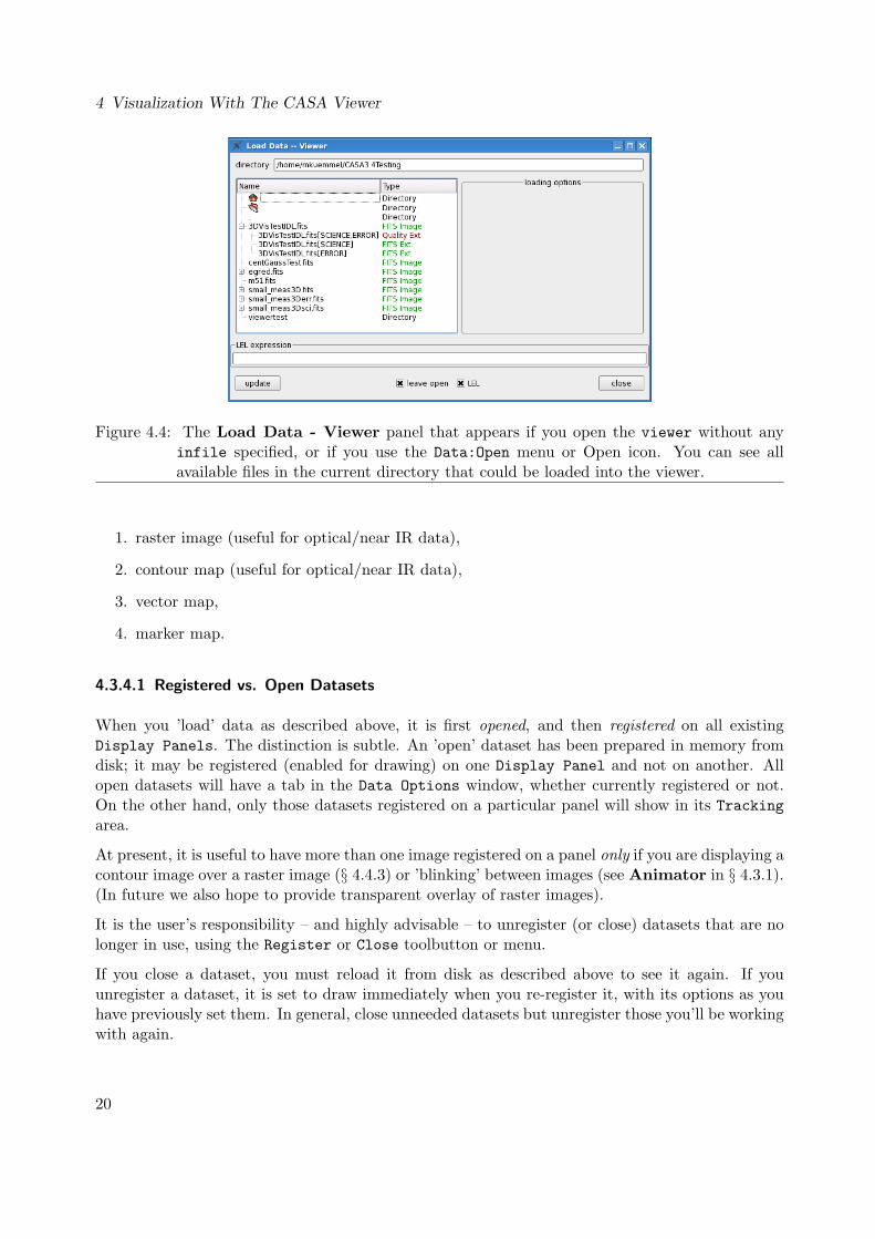
You can use the Load Data - Viewer GUI to interactively choose images to load into the viewer.An example of this panel is shown in Figure 4.4. This panel is accessed through the Data:Openmenu or the Open icon of the Viewer Display Panel (see Fig. 4.2). It also appears if you openthe viewer without any infile specified. In addition to the home and the root directories the loaddata panel shows the files that could be loaded into the viewer (images and restore files) and thesub-directories of the current directory. FITS images with several extensions are show with a +-sign(grey arrow on MacOSX) that can be expanded. In the expanded view, the FITS extensions ofan image are shown with their extension name and extension version (if available) as type ‘‘FITSext.’’.

The document VLT-SPE-ESO-19500-5667 describes a way of storing science data and its pixel-by-pixel error in separate extensions of a FITS file. In the load data panel, such a pair of data-errorextensions have the type Quality Ext. and are shown with their combined extension names (seeFig. 4.4). Loading a Quality Extension into the viewer means loading both, the data and the errorvalues. In the spectral profiler the error values are used to e.g. overplot the data values (see § 4.5).

Selecting a file on disk in the Load Data panel will provide options for how to display the data.Images can be displayed as (see § 4.4 for details):

19


Figure 4.4: The Load Data - Viewer panel that appears if you open the viewer without anyinfile specified, or if you use the Data:Open menu or Open icon. You can see allavailable files in the current directory that could be loaded into the viewer.

1. raster image (useful for optical/near IR data),

2. contour map (useful for optical/near IR data),

3. vector map,

4. marker map.

4.3.4.1 Registered vs. Open Datasets

When you ’load’ data as described above, it is first opened, and then registered on all existingDisplay Panels. The distinction is subtle. An ’open’ dataset has been prepared in memory fromdisk; it may be registered (enabled for drawing) on one Display Panel and not on another. Allopen datasets will have a tab in the Data Options window, whether currently registered or not.On the other hand, only those datasets registered on a particular panel will show in its Trackingarea.

At present, it is useful to have more than one image registered on a panel only if you are displaying acontour image over a raster image (§ 4.4.3) or ’blinking’ between images (see Animator in § 4.3.1).(In future we also hope to provide transparent overlay of raster images).

It is the user’s responsibility – and highly advisable – to unregister (or close) datasets that are nolonger in use, using the Register or Close toolbutton or menu.

If you close a dataset, you must reload it from disk as described above to see it again. If youunregister a dataset, it is set to draw immediately when you re-register it, with its options as youhave previously set them. In general, close unneeded datasets but unregister those you’ll be workingwith again.

20

4.4 Viewing Images

Figure 4.5: The Save Data - Viewer panel that appears when pressing the ’save data’ icon inthe Main Toolbar (Figure 4.2).

4.3.5 The Save Data Panel

The user can use the Save Data - Viewer GUI to export images from the viewer to a file. Thepanel is shown Figure 4.5. This panel is opened with the Data:Save as menu or pressing the’Save Data’ icon in the Main Toolbar (Figure 4.2). The upper part lists all images that can beexported to disk. To save an image to a file, the user can either enter the new filename in the boxlabeled ’save to:’ followed by the save-button (alternatively the ’Enter’-key), or press ’browse...’and specify a filename via a standard filebrowser GUI.

Independent on the original format, images can be exported in both, FITS format and CASA imageformat.

4.4 Viewing Images

There are several options for viewing an image. These are seen at the right of the Load Data -Viewer panel described in § 4.3.4 and shown in Figure 4.6 after selecting an image. They are:

• raster image — a greyscale or color image,

• contour map — contours of intensity as a line plot,

• vector map — vectors (as in polarization) as a line plot,

• marker map — a line plot with symbols to mark positions.

21


Figure 4.6: The Load Data - Viewer panel as it appears if you select an image. You can see alloptions are available to load the image as a raster image, contour map, vector map,or marker map. In this example, clicking on the raster image button would bring upthe displays shown in Figure 4.1.

The raster image is the default image display, and is what you get if you invoke the viewer fromcasapy with an image file name. In this case, you will need to use the Open menu to bring up theLoad Data panel to choose a different display.

4.4.1 Viewing a raster map

A raster map of an image is the normal mode to display an image. Here the pixel intensities areshown in a two-dimensional cross-section of gridded data with colors selected from a finite set of(normally) smooth and continuous colors, i.e., a colormap.

Starting the casaviewer with an image as a raster map will look something like the example inFigure 4.1.

You will see the GUI which consists of two main windows, entitled ”Viewer Display Panel” and”Load Data”. In the ”Load Data” panel, you will see all of the viewable files in the current workingdirectory along with their type. After selecting a file, you are presented with the available displaytypes (raster, contour, vector, marker) for these data. Clicking on the button raster image willcreate a display Fig. 4.1.

The data display can be adjusted by the user as needed. This is done through the Data Dis-play Options panel. This window appears when you choose the Data:Adjust menu or use thespanner/wrench icon from the Main Toolbar.

The Data Display Options window is shown in the right panel of Figure 4.1. It consists of a tabfor each image or MS loaded, under which are a cascading series of expandable categories. For animage, these are:

22

4.4 Viewing Images

Figure 4.7: The hidden axis category of the Data Display Options panel as it appears if youload data and error values stored in two image extensions. For a quality axis slider tothe left and right displays the data and error values, respectively.

• display axes

• hidden axes

• basic settings

• position tracking

• axis labels

• axis label properties

• color wedge

The basic settings category is expanded by default. To expand a category to show its options,click on it with the left mouse button.

4.4.1.1 Raster image — display axes

In this category the physical axes (i.e. Right Ascension, Declination, Velocity, Stokes) to be dis-played can be selected and assigned to the x, y, and z axes of the display.

4.4.1.2 Raster image — hidden axes

Since the viewer can only show three axes of an image (in x- y- and z-axis of the display), imageswith more than three axes need a selection mechanism for the axes that can not fully be displayed.This selection mechanism is in the hidden axes drop-down. For each additional axis a slider allowsto select the plane displayed. Such hidden axes could be the “quality axis” if data and error valuesare loaded. Figure 4.7 shows the slider for a quality axis. Slider to the left (0) displays the datavalues, slider to the right shows the error values.

23


Figure 4.8: The basic settings category of the Data Display Options panel as it appears ifyou load the image as a raster image. This is a zoom-in for the data displayed inFigure 4.1.

4.4.1.3 Raster image — basic settings

This roll-up is open by default. It has some commonly-used parameters that alter the way theimage is displayed; three of these affect the colors used. An example of this part of the panel isshown in Figure 4.8.

The options available are:

• basic settings: aspect ratio

This option controls the horizontal-vertical size ratio of data pixels on screen. fixed world(the default) means that the aspect ratio of the pixels is set according to the coordinate systemof the image (i.e., true to the projected sky). fixed lattice means that data pixels willalways be square on the screen. Selecting flexible allows the map to stretch independentlyin each direction to fill as much of the display area as possible.

• basic settings: pixel treatment

This option controls the precise alignment of the edge of the current ’zoom window’ withthe data lattice. edge (the default) means that whole data pixels are always drawn, even onthe edges of the display. For most purposes, edge is recommended. center means that datapixels on the edge of the display are drawn only from their centers inwards. (Note that adata pixel’s center is considered its ’definitive’ position, and corresponds to a whole numberin ’data pixel’ or ’lattice’ coordinates).

• basic settings: resampling mode

This setting controls how the data are resampled to the resolution of the screen. nearest (thedefault) means that screen pixels are colored according to the intensity of the nearest datapoint, so that each data pixel is shown in a single color. bilinear applies a bilinear interpo-lation between data pixels to produce smoother looking images when data pixels are large onthe screen. bicubic applies an even higher-order (and somewhat slower) interpolation.

24

4.4 Viewing Images

• basic settings: data range

You can use the entry box provided to set the minimum and maximum data values mappedto the available range of colors as a list [min, max]. For very high dynamic range images,you will probably want to enter a max less than the data maximum in order to see detail inlower brightness-level pixels. The next setting also helps very much with high dynamic rangedata.

• basic settings: scaling power cycles

This option allows logarithmic scaling of data values to colormap cells.

The color for a data value is determined as follows: first, the value is clipped to lie within thedata range specified above, then mapped to an index into the available colors, as describedin the next paragraph. The color corresponding to this index is determined finally by thecurrent colormap and its ’fiddling’ (shift/slope) and brightness/contrast settings (see MouseToolbar, above). Adding a color wedge to your image can help clarify the effect of thevarious color controls.

The scaling power cycles option controls the mapping of clipped data values to colormapindices. Set to zero (the default), a straight linear relation is used. For negative scalingvalues, a logarithmic mapping assigns an larger fraction of the available colors to lower datavalues (this is usually what you want). Setting dataMin to something around the noise levelis often useful/appropriate in conjunction with a negative ’power cycles’ setting.

For positive values, an larger fraction of the colormap is used for the high data values1.

See Figure 4.9 for sample curves.

• basic settings: colormap

You can select from a variety of colormaps here. Hot Metal, Rainbow and Greyscale col-ormaps are the ones most commonly used.

4.4.1.4 Raster image — position tracking

Contains settings for the position tracking box (Sect. 4.3.1), e.g. the units of the spectral values .

4.4.1.5 Raster image — axis labels

Settings for axis labelling in the main viewer, e.g. to add a title or give dedicated axis labels. Thesesetting might be especially relevant when generating to create publication-ready plots.

1The actual functions are computed as follows:For negative scaling values (say −p), the data is scaled linearly from the range (dataMin – dataMax) to the

range (1 – 10p). Then the program takes the log (base 10) of that value (arriving at a number from 0 to p) andscales that linearly to the number of available colors. Thus the data is treated as if it had p decades of range,with an equal number of colors assigned to each decade.

For positive scaling values, the inverse (exponential) functions are used. If p is the (positive) value chosen, Thedata value is scaled linearly to lie between 0 and p, and 10 is raised to this power, yielding a value in the range(1 – 10p). Finally, that value is scaled linearly to the number of available colors.

25


Figure 4.9: Example curves for scaling power cycles.

4.4.1.6 Raster image — axis label properties

Many settings in this sections address the layout of the axis labels, such as the label color and thefont size, which are important when generating dedicated plots, e.g. for publications.

Other settings control the units shown in the main viewer (see Figure 4.10)

• axis label properties: world or pixel coordinates

Showing the x- and y-axis of the main viewer either in world or pixel coordinates.

• axis label properties: direction reference

The reference system for the directional coordinate. Possible choices are J2000, B1950,GALACTIC, ECLIPTIC and SUPERGAL independent on the reference system associated to theimage coordinates.

• axis label properties: spectral reference

The reference system for the spectral coordinate.

• axis label properties: spectral unit

The unit for the spectral coordinate. Available are many units in the frequency, velocity(optical and radio 2), wavelength and air wavelength domain. Selecting a velocity unit isonly reasonable if a rest frequency is given in the setting axis label properties: restfrequency or wavelength, either with user input or via the image metadata.

2There are two velocity definitions in use in radio astronomy. The “radio” definition, used in Galactic radioastronomy is vr = ν0−ν

ν0c. the “optical” definition, used throughout extragalactic astronomy is vo = ν0−ν

νc =

λ−λ0λ0

c = zc. Neither optical, nor radio velocities represent physical quantities; they are merely approximations of

the full relativistic expressions for small velocities (< 1000 km s−1)

26

4.4 Viewing Images

Figure 4.10: Selected settings from the axis label properties category of the Data DisplayOptions panel. These options control the units on all displayed axes.

• axis label properties: movie axis label type

Showing the z-axis (or movie-axis) of the main viewer either in world or pixel coordinates.

• axis label properties: movie axis label position

The position of the movie axis label. Available are four positions inside an four positionsoutside of the pixel image.

4.4.1.7 Raster image — color wedge

Settings to give add a color wedge in the main display.

4.4.2 Viewing a contour map

Viewing a contour image is similar to the process above. A contour map shows lines of equal datavalue (e.g., flux density) for the selected plane of gridded data (Figure 4.11). Contour maps areparticularly useful for overlaying on raster images so that two different measurements of the samepart of the sky can be shown simultaneously (§ 4.4.3).

Several basic settings options control the contour levels used. The contours themselves arespecified by a list in the box Relative Contour Levels. These are defined relative to the two other

27


Figure 4.11: The Viewer Display Panel (left) and Data Display Options panel (right) afterchoosing contour map from the Load Data panel. The image shown is for channel500 of the cube 3DVisTestIDL.fits, selected using the Animator tape deck. Notethe different options in the open basic settings category of the Data DisplayOptions panel (as compared to raster image in Figure 4.1).

parameters, the Base Contour Level (which sets what 0 in the relative contour list correspondsto in the image), and the Unit Contour Level (which sets what 1 in the relative contour listcorresponds to in the image). Note that negative contours are usually dashed.

For example, it is relatively straightforward to set fractional contours (e.g. “percent levels”), e.g.:

Relative Contour Levels = [0.01, 0.05, 0.2, 0.4, 0.6, 0.8]Base Contour Level = -10.0Unit Contour Level = <image max>

This maps the maximum to 1 and thus our contours are fractions of the peak.

Another example shows how to set absolute values so that the contours are given in image units:

Relative Contour Levels = [10, 100, 1000, 1900]Base Contour Level = 0.0Unit Contour Level = 1.0

Here we have contours at 10, 100, 1000 and 1900.

We can also set contours in multiples of the image rms (“sigma”):

Relative Contour Levels = [-3,3,5,10,15,20]

28

4.5 Spectral Profile Plotting

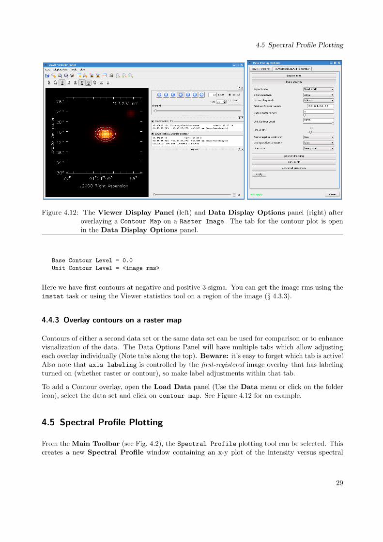
Figure 4.12: The Viewer Display Panel (left) and Data Display Options panel (right) afteroverlaying a Contour Map on a Raster Image. The tab for the contour plot is openin the Data Display Options panel.

Base Contour Level = 0.0Unit Contour Level = <image rms>

Here we have first contours at negative and positive 3-sigma. You can get the image rms using theimstat task or using the Viewer statistics tool on a region of the image (§ 4.3.3).

4.4.3 Overlay contours on a raster map

Contours of either a second data set or the same data set can be used for comparison or to enhancevisualization of the data. The Data Options Panel will have multiple tabs which allow adjustingeach overlay individually (Note tabs along the top). Beware: it’s easy to forget which tab is active!Also note that axis labeling is controlled by the first-registered image overlay that has labelingturned on (whether raster or contour), so make label adjustments within that tab.

To add a Contour overlay, open the Load Data panel (Use the Data menu or click on the foldericon), select the data set and click on contour map. See Figure 4.12 for an example.


From the Main Toolbar (see Fig. 4.2), the Spectral Profile plotting tool can be selected. Thiscreates a new Spectral Profile window containing an x-y plot of the intensity versus spectral

29


Figure 4.13: The Spectral Profile panel (right) that appears when pressing the button Open theSpectrum Profiler in the Main Toolbar and then use the tools to select a regionin the image, such as the rectangular region on the left panel. The profile changes totrack movements of the region if moved by dragging with the mouse.

axis. The displayed spectrum is extracted in region marked with the Point, Rectangle, Ellipseor Polygon Region tool in the Viewer Display Panel. The spectrum shown in the SpectralProfile window (right panel in Figure 4.13) is automatically updated if the corresponding regionis dragged across the image in the Viewer Display Panel (right panel in Fig. 4.13).

4.5.1 Toolbar

The toolbar of the Spectral Profile (Figure 4.14) contains action icons to (from left to right):

• save data - export the current profile to a FITS or ASCII file;

• print - print the main window;

• save panel - save the panel as an image (PNG, JPG, PDF, ...);

• preferences - set plot preferences;

• move left - ’move’ the x-boundaries of the spectrum plot to the left;

• move right - ’move’ the x-boundaries of the spectrum plot to the right;

• move up - ’move’ the y-boundaries of the spectrum plot up;

• move down - ’move’ the y-boundaries of the spectrum plot down;

• zoom reset - reset the zoom;

30


Figure 4.14: The toolbar of the Spectral Profile contains a couple of action icons to save data ormanipulate the displayed xy-range.

• zoom in - zoom in;

• zoom out - zoom out;

Figure 4.15 shows the panel with the plot preferences. Several settings can be switched on/off:

• x Auto Scale: adjust the x-boundaries dynamically;

• y Auto Scale: adjust the y-boundaries dynamically;

• Show Grid: connect the tickmarks with lines;

• Overlay: extract and plot the spectra of all cubes registered in the viewer;

• Top Axis: show units on the top axis.

Figure 4.15: The plot preferences panel

4.5.2 Main window

The main window shows the spectrum extracted from the image. The unit of the spectral axis canbe selected between frequency, wavelength and velocity units. Velocity units are only available ifa rest frequency is defined (see Sect. 4.4.1.6). The user can choose between the different combinetypes mean, median and sum in a combo box. The spectra are scaled in the y-axis to avoid numbersthat long and difficult to decipher. The scaling is expressed in prefix letter to the y-axis unit(m = 10−3, k = 103, M = 106, . . . ; see e.g. Fig. 4.16).

31


Figure 4.16: With dragging the left mouse button over the main window the user can inter-actively modify the plot boundaries in x and y and thus zoom in or out the profile(yellow box in left panel).

Besides the spectral values also the error bars can be plotted. There are two different ways toderive error values, which are set inn a combo box. If the region used for the extraction has twodimensions (rectangle, ellipse and polygon), for each spectral channel the root-mean squared errorcan be computed and used as error (error type rmse in the combo box). If both, the data valuesand the pixel-by-pixel error values had been loaded into the viewer as a Quality Extension (seeSect. 4.3.4), these error values are used for the error bars (error type propagated in the combobox). For a point-region, the error values are directly plotted as error bars, for rectangle, ellipseand polygon the pixel errors are, at each wavelength, propagated to determine a single error valuewhich overplot the data value.

The main window is sensitive to the following combination input from keyboard and mouse (Figure4.18):

• zoom: When pressing and dragging the left mouse button, a yellow box is drawnonto the panel. After releasing the mouse button, the xy-range is zoomed to the values ofthe yellow box (see Figure 4.16). The sensitive area includes the regions outside the currentplotting boundaries, thus it is also possible to zoom out.

• spectral range selection: When pressing and dragging left mouse button with shift-key,a gray box marks a spectral range in the plot, as shown in Figure 4.17. The start and endvalues are written into the from: and to: box of the collapse/moments and linefit tab.This allows an interactive selection of the spectral range used in the collapse/moments or

32


Figure 4.17: Pressing the shift-key while dragging the left mouse button marks a spectralrange with a gray area (middle panel) and provides start and end values for the tabscollapse/moments and linefit.

linefit operation;

• spectral channel selection: When pressing the ctrl-key, a gray line is drawn at thecurrent position of the mouse in the spectral profile window (Fig. 4.18). After pressing theleft mouse button, the image in the Viewer Display Panel displays in the z-axis thespectral channel marked with the gray line.

4.5.3 Spectral/Image analysis

The two tabs labeled Collapse/Momentsand Spectral-Line Fitting in the lower part of theSpectral Profile panel offer simple image analysis tools to the user (see Figs. 4.17 and 4.19).

In Collapse/Moments the user can collapse the image along the spectral axis between the start andend values provided in the corresponding boxes. Various collapse types (mean, median and sum) areoffered, and the error is computed via error propagation from the pixel errors propagated or bycomputing the root-mean squared error (rmse). The collapsed image is displayed in the ViewerDisplay Panel.

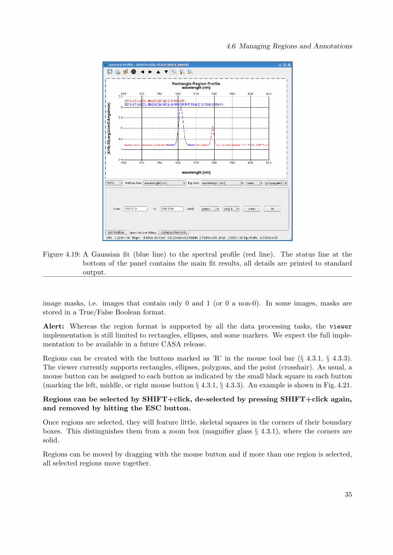
In Sepctral-Line Fitting the user can fit a function to the to the spectrum profile (Figure 4.19).A Gaussian plus a polynome of up to first (linear) order can be selected for the fit function intwo combo boxes. If error bars are displayed in the spectral profiler, they are used in the fittingas weights. The main results of the fit are shown in the status bar of the Spectral Profile. A

33


Figure 4.18: With the ctrl-key pressed, a gray line marks the cursor position. Clicking the leftmouse button displays the corresponding spectral channel in the Viewer DisplayPanel.

detailed summary of the fit is sent to the standard output (either the casapy window or the windowwhere the viewer was started).

4.5.4 Set Position

The third tab labeled Set Position in the lower part of the Spectral Profile panel offers a non-interactive way of extracting spectra from the 3D cube loaded in the main viewer. The coordinates(absolute and pixel) of point and rectangular region are inserted into the GUI elements. Whenpressing the button Apply, the spectrum is extracted and displayed in the main window of theprofiler. The operation does not create a corresponding region in the region panel of the mainviewer.

4.6 Managing Regions and Annotations

CASA regions are following the CASA ’crtf’ standard as described in the CASA User Reference& Cookbook. CASA regions can be used in all applications, including clean and image analysistasks of CASA . In addition, a leading ’ann’ to each region definition indicates that it is for visualoverlay purposes only. On a side note: apart from the regions mentioned here, CASA supports

34


Figure 4.19: A Gaussian fit (blue line) to the spectral profile (red line). The status line at thebottom of the panel contains the main fit results, all details are printed to standardoutput.

image masks, i.e. images that contain only 0 and 1 (or 0 a non-0). In some images, masks arestored in a True/False Boolean format.

Alert: Whereas the region format is supported by all the data processing tasks, the viewerimplementation is still limited to rectangles, ellipses, and some markers. We expect the full imple-mentation to be available in a future CASA release.

Regions can be created with the buttons marked as ’R’ in the mouse tool bar (§ 4.3.1, § 4.3.3).The viewer currently supports rectangles, ellipses, polygons, and the point (crosshair). As usual, amouse button can be assigned to each button as indicated by the small black square in each button(marking the left, middle, or right mouse button § 4.3.1, § 4.3.3). An example is shown in Fig. 4.21.

Regions can be selected by SHIFT+click, de-selected by pressing SHIFT+click again,and removed by hitting the ESC button.

Once regions are selected, they will feature little, skeletal squares in the corners of their boundaryboxes. This distinguishes them from a zoom box (magnifier glass § 4.3.1), where the corners aresolid.

Regions can be moved by dragging with the mouse button and if more than one region is selected,all selected regions move together.

35


Figure 4.20: Extracting a spectrum with the Set Position tab. The pixel coordinates of the pointregion ((x, y) = (15, 15)) is specified in the GUI elements.

To load, unload, modify, and to display the value statistics of each region, the Region Panel canbe loaded via the ’View’→’region’ drop-down menu. As all other panels, the region panel can bedocked to different portions of the viewer and it can also be detached. If it is dismissed (the crossin the upper right corner), it can be retrieved by the ’View’ menu.

The three basic windows of the region panel are shown in Fig. 4.22.

4.6.1 Region Panel: properties

The properties tab can be used to adjust the the size, center, and coordinate frame of the region(’coordinates’ selection at the top). The inputs can be in different units, and those implementedin the viewer are commonly used sub-sets of the options listed in the CASA User Reference &Cookbook. At the top of the panel, one can specify the channel range over which the region shallbe defined. The ’selection’ check box is an alternative way to the SHIFT+click to select aregion. The ’annotation’ checkbox will place the ’ann’ string in front of the region ascii output– annotation regions are not be used for processing in, e.g. data analysis tasks.

The second horizontal tab ’line’ brings up a panel to change the color, line width, and line style(solid, dotted, dashed) of the selected region.

36


Figure 4.21: Image regions created with the region tools of the viewer. The region panel is shownto the right.

The third panel, ’text’, can be used to assign a string to the region which can be controlled inposition (the little dial at the bottom, and the two right hand boxes), as well as text font, style,and color.

4.6.2 Region Panel: stats

The second vertical tab, ’stats’, displays the statistics of each region. When more than a singleregion is drawn, one can select them one by one and the region panel updates image information andvalue statistics for each region. The informational section contains the frequency, velocity, stokesand brightness unit of the image. The beam area is also calculated from the header informationof the image. The statistical properties of the pixels within in the region comprises the number ofpixels (Npts), the Sum, Mean, RMS, Minimum, and Maximum of the pixel values, as well as theimage flux integrated over the region. All values are updated on the fly when the region is draggedacross the image.

Note that double-clicking the region will output the statistics to the terminal as explained above.This is an easy way to copy and paste the statistical data to a program outside of CASA for furtheruse.

37


Figure 4.22: The four vertical tabs of the region panel: properties, stats, fit, and file.

4.6.3 Region Panel: fit

The third tab ’fit’ is used for fitting 2D Gaussians to the pixels values enclosed in the rectan-gle, ellipse or polygon region. Figure 4.23 illustrates the Gaussian fitting. Pressing the buttongaussfit executes the fit with the option of taking into account a constant sky level in the boxsky component. The fitting results are written to the terminal and to the region panel (both inpixel and world coordinates). The center coordinates and the position angle can be overlayed inthe main image (left side of Fig. 4.23) using a color chosen by the user.

If a region is modified or moved, or a different layer in z is shown, the fitted values are no longervalid. As a consequence the overlay of the center and position angle is removed and the fit resultsin the panel are shown with a dark background.

4.6.4 Region Panel: file

The fourth tab ’file’ is used for loading and saving regions from and to disk (select the appropriatethe action at the top). To save to ascii file, one can specify the file format, where the default is

38


Figure 4.23: 2D Gaussian fitting in regions. The fit results are written to the terminal, shown inthe region panel and overlaid in the image (left).

a CASA region file (saved with a *.crtf suffix, see the CASA User Reference & Cookbook.It isalso possible to load and save DS9 regions, but remember that the DS9 format does not offer thefull flexibility and cannot capture stokes and spectral axes. DS9 regions will only be usable asannotations in the viewer, they cannot be used for data processing in other CASA tasks.

When saving regions, one can also specify whether to save only the current region, all regions thatwere selected with SHIFT+click, or all regions that are visible on the screen.

39


40

Index

3D visualization tool, 8, 9

Animator panel, 17axis label properties, 26axis labels, 25

CASA, 8, 9download, 10ESO release, 9image format, 12installation, 10region, 34release, 9User Reference & Cookbook, 8, 12viewer, 8, 9

CASA:image format, 21casapy, 10, 12casaviewer, 10, 12, 22Collapse/Moments, 33contour map, 20, 21, 27

Data Display Options, 13, 22Display Area, 17display axes, 23distance tool, 17

ellipse region, 16, 30, 32error, 32

propagated, 32rmse, 32

error typepropagated, 33

error typermse, 42

ESO, 8extension name, 12extension version, 12

FITS format, 21FITS image, 12

Gaussian1D, 33

Gaussian 2D, 38, 39

hidden axes, 23

image region, 19installation, 9

Linux, 10MAC OS, 11

Linux, 9Load Data - Viewer, 19, 20

Mac OS, 910.6, 910.7, 9

Main Toolbar, 15mouse button, 15Mouse Tool, 15, 16MUSE, 8

NaN, 13

open dataset, 20

Panel StateRestore, 18Save, 18

plot preferences, 31point region, 16, 30, 32polygon region, 16, 19, 30, 32polynome, 33Position Tracking panel, 17preferences

file, 12propagated, 33

Quality Extension, 19, 32

raster image, 20–22

41

Index

rectangle region, 16, 18, 30, 32region stats, 37registered dataset, 20rmse, 32rmse, 33root-mean squared error, 32, 33

Save Data Panel, 21scaling, 31Set Position, 34SINFONI, 8spectral channel selection, 33Spectral Profile panel, 19, 29, 30spectral range selection, 32Spectral-Line Fitting, 33support, 11

Viewer Display Panel, 13, 14, 19viewer task, 12VLT

instruments, 8

42

very large telescope 3d visualization tool manual · very large telescope 3d visualization tool...

Documents