virtual sculpting: an investigation of directly manipulated free … · b directly manipulated...

Virtual Sculpting: An Investigation of Directly

Manipulated Free-Form Deformation in a Virtual

Environment

THESIS

Submitted in fulfilment of the requirements

for the Degree of

MASTER OF SCIENCE

of Rhodes University

by

James Edward Gain

February 1996

Abstract

This thesis presents a Virtual Sculpting system, which addresses the problem of Free-Form

Solid Modelling. The disparate elements of a Polygon-Mesh representation, a Directly

Manipulated Free-Form Deformation sculpting tool, and a Virtual Environment are drawn

into a cohesive whole under the mantle of a clay-sculpting metaphor. This enables a

user to mould and manipulate a synthetic solid interactively as if it were composed of

malleable clay. The focus of this study is on the interactivity, intuitivity and versatility of

such a system. To this end, a range of improvements is investigated which significantly

enhances the efficiency and correctness of Directly Manipulated Free-Form Deformation,

both separately and as a seamless component of the Virtual Sculpting system.

Acknowledgements

My supervisors, Professor Dave Sewry and Professor Peter Clayton, have with their help-

fulness, interest and cross-questioning made my research at Rhodes University stimulating

and fruitful.

I have spent many an hour with pencil or chalk explaining my work to fellow postgraduates.

My thesis has benefitted from the probing and challenging discussions that followed. The

members of the RhoVeR development team have helped build the Virtual Reality system

that I incorporated into this work, and for this I am extremely grateful.

My family have always provided a constant background of encouragement and bolstering,

even when they did not understand why I always seemed to be playing with black Lycra

gloves and visorless helmets.

Ingrid van Eck has many times rightly felt that she was writing this thesis alongside me.

Without her by my side, proofreading over my shoulder, "surfing the net" while I worked,

occasionally "cracking the whip" and always giving love and patient support, this thesis

would have been an insurmountable task.

Thanks also are due to my proofreading "team": Shaun Bangay, Prof. Peter Clayton, Prof.

Dave Sewry, Ingrid van Eck and Greg Watkins, who have dissected the mathematics and

grammar of this thesis.

I acknowledge the financial support of Rhodes University and the Foundation for Research

Development.

Trademark Information:

The following are registered trademarks: 5thGlove, InsideTRAK, IsoTRAK, Linux, Lycra,

OpenGL, Pixel-Plane, Plasticine, Polhemus, Solaris, SPARCServer, SunOS and Unix.

1

Contents

1 Introduction 6

1.1 Solid Modelling �� 6

1.2 Classification of Modelling Systems �� 7

1.2.1 Representation �� 7

1.2.2 Tools �� 8

1.2.3 Environment �� 9

1.3 Polygon-Mesh Representation �� 10

1.4 Sculpting Tools �� 10

1.5 Virtual Environments �� 12

1.6 Focus of Research �� 14

1.7 Thesis Organisation �� 15

2 Foundations 16

2.1 Splines �� 16

2.1.1 Uniform Rational Basis-Splines �� 17

2

2.1.2 Other Splines �� 21

2.2 Free-Form Deformation �� 21

2.3 Direct Manipulation �� 27

2.4 Concluding Remarks �� 31

3 Least Squares Solution Methods 32

3.1 Theoretical Underpinnings �� 33

3.1.1 Systems of Linear Equations �� 33

3.1.2 The Pseudo-inverse �� 34

3.2 Solution Schemes �� 37

3.2.1 Naıve Pseudo-inverse �� 37

3.2.2 Method of Normal Equations �� 39

3.2.3 Greville’s Method �� 41

3.2.4 Householder QR Factorization �� 44

3.2.5 Evaluation �� 47

3.3 Direct Manipulation Specifics �� 48


4 Topology and Correctness Issues 56

4.1 Definition of Terms �� 56

4.2 Self-Intersection �� 58

4.3 Refinement �� 60

3

4.3.1 Splitting Criterion �� 61

4.3.2 Subdivision Methods �� 62

4.4 Decimation �� 64


5 Applications 70

5.1 RhoVeR �� 70

5.2 The Virtual Sculpting Testbed �� 71

5.3 Interactive Surface Sketching �� 73

5.4 Glove-based Moulding �� 76


6 Conclusion 79

6.1 Conclusions �� 79

6.2 Future Work �� 80

6.2.1 Replacing the Underlying Splines �� 81

6.2.2 Complex Lattices �� 81

6.2.3 Analysis of Self-Intersection �� 82

6.2.4 Piercing Holes in the Solid �� 82

6.2.5 Further Applications �� 82

A Colour Plates 84

4

B Directly Manipulated Free-Form Deformation Program Extracts 87

C Specification of the RhoVeR System 101

C.1 Overview �� 101

C.2 Interprocess Communication Facilities �� 102

C.2.1 Event-passing �� 102

C.2.2 The virtual shared memory �� 102

C.3 The global data structures �� 102

C.3.1 The distributed data base �� 102

C.3.2 The shape data �� 103

C.3.3 Local values �� 103

C.4 The modules �� 103

C.4.1 The communication modules �� 104

C.4.2 The World Control modules �� 105

C.4.3 Output Modules �� 106

C.4.4 Input Modules �� 106

C.5 Event-passing �� 106

C.5.1 Send Event �� 106

C.5.2 Get Event and GetMatchingEvent �� 107

5

Chapter 1

Introduction

1.1 Solid Modelling

Solid Modelling is a significant subdiscipline of Computer Graphics concerned with de-

signing three-dimensional objects on computer. The field has diverse applications, both in

manufacturing, where, under the guise of Computer Aided Design (CAD), it is pervasive,

and as a component in most Computer Graphics creation pipelines. For instance, it is

critical to the design of cars, ships and aircraft, complex mechanical parts and architectural

structures, as well as Computer Animated models and Virtual Reality scenes. These two

spheres mirror the division of Solid Modelling into functional and free-form [Miller 1986].

Free-Form Modelling is concerned only with the aesthetics of the final shape. In contrast,

Functional Modelling considers factors such as aerodynamics, joint angles, volume, and

response to heat and stress, typically through mechanisms such as Finite Element Analysis.

This is not, however, a clear separation so much as a continuum of constraint. At one pole,

a computer sculptor is influenced only by his imagination and at the other, a gear train

may have to satisfy a plethora of constraints. Alternatively, the design of a motor vehicle’s

shell, which must link engineering considerations with a nebulous sleekness, would fall

somewhere in between.

6

Free-Form Solid Modelling is guided by three criteria:

1. Intuitivity. The user should be able to apply insight garnered from everyday tasks to

an unfamiliar modelling environment.

2. Interactivity. The response-time of the system should be such that delays do not

hinder creative design.

3. Versatility. The user should be able to convert intentions and requirements into a

designed result with ease and precision.

These principles exist in constant tension. Focusing on one aspect tends to wrench the

others out of balance. Enhanced versatility, for example, may increase conceptual and

computational complexity to the detriment of the intuitive and interactive facets of a system.

During construction, a modelling system must be measured constantly against these ideals.

1.2 Classification of Modelling Systems

Free-Form Solid Modellers can be separated into three components: Representation, Tools

and Environment. These correspond loosely to data-structures, algorithms and interfaces.

1.2.1 Representation

A Representation is a means of encoding the shape of a solid object. Some modelling

systems may capture properties such as colour and texture, but for free-form design, shape

is sufficient. There are four principle categories of representations [Foley et al 1991]:

1. Boundary Representations (B-Reps). Here, an object is defined by its topological

boundary and the internal structure is ignored. B-Reps may be either Polyhedral,

where the surface is a faceted approximation composed of adjoining polygons, or

Non-Polyhedral, where the surface is sewn from parametric bicubic patches. The

Polygon-Mesh is an example of a Polyhedral B-Rep. At its most elementary it

7

consists of a list of faces, each of which is a sequence of pointers into a vertex list.

In contrast, the popular Non-Uniform Rational B-Spline (NURBS) supports a Non-

Polyhedral B-Rep. A NURBS patch is tersely defined by a web of control points

much as an elastic sheet is distorted by weights.

2. Cell Decomposition. The solid is formed by "glueing" together primitive elements

which are themselves solids that may vary in size, shape and orientation. For example,

Spatial Occupancy Enumeration is a variant in which all the primitives are identical

cubes known as Voxels (Volume Elements) in analogy to Pixels (Picture Element).

These Voxels can be visualized as slotting into compartments in a three-dimensional

grid.

3. Constructive Solid Geometry (CSG). Again a solid is built from primitives (spheres,

cylinders, etc.) but instead of simple non-intersecting adjacency they are combined

with Regularized Boolean Set Operations (union, intersection and difference). Typ-

ically CSG solids are stored as a tree structure, where the leaf nodes are primitives,

internal nodes are set operations, and the root solid is evaluated by a depth-first walk.

4. Binary Space Partitioning (BSP). Here a solid is sliced out of world co-ordinate

space. Each slice is created by a plane which partitions space into two domains, one

within and the other outside the solid.

1.2.2 Tools

A tool metaphor is unusually appropriate when referring to methods of transforming solids.

A direct comparison can be made with a craftsman’s use of a range of tools in realizing a

design. A solid modeller would select techniques on the basis of the solid’s representation

and desired shape, just as a craftsman would employ different tools depending on his

materials and intentions.

Solid Modelling tools can be placed in three categories [Coquillart 1987]:

1. Modifiers. Modifiers are tools that perturb the shape of an existing object, either

within a limited area, or across the object’s entirety. Examples of the latter are the

8

tapering, twisting and bending tools [Barr 1984]. These are proportional applications

of the affine transformations (scaling, rotation and translation). By contrast, free-form

surface moulding falls in the former category and is a staple of Solid Modelling. At

its most primitive it involves displacing individual vertices and at its most advanced

it allows complex widespread deformations.

2. Combiners. These methods create a synthesis of objects. Foremost among them

are the Regularized Boolean Set Operations: Union, Intersection and Difference.

These are three-dimensional analogues of the familiar two-dimensional set opera-

tions, extended so as to encompass solids. Regularized Boolean Set Operations are

supported across the spectrum of Solid Modellers and their use is even mandated by

representations such as Constructive Solid Geometry.

3. Constructors. Unlike the other classes of tools that modify previously developed

objects, constructors build solids from nothing. At its most painstaking this entails

entering vertex co-ordinates directly and expecting the computer to interpolate these

values in creating a solid. Fortunately, there are less excruciating constructors such as

primitive instancing, sweeping and lofting. Primitive instancing allows the selection

of one of a family of parametrised three-dimensional primitives. A sweep object is

constructed by sliding a two-dimensional contour along a curved path, with a goblet

or wine glass being a typical result. Lofting forms objects by interpolating a series of

cross-sections and is often applied to the definition of hulls, fuselages and car-bodies.

1.2.3 Environment

There is a strong symbiotic relationship between Solid Modelling and Human Com-

puter Interaction, with each discipline feeding off innovations in the other. This is

probably because the design of three-dimensional shapes is an inherently difficult task

[Requicha and Rossignac 1992] which involves the user directly. Thus, design environ-

ments vary as widely as their application domains, and the range in IO devices and interac-

tion styles is bewildering. Fortunately, modelling systems can be separated at a fundamental

level into two classes:

9

1. Two-Dimensional. Interaction is funnelled through two-dimensional media. A

typical interface would accept input from a mouse or light-pen and output a set of

orthogonal views.

2. Three-Dimensional. The environment is controlled by and responds with three-

dimensional mechanisms. Such systems are generally driven by six-degree-of-

freedom devices and display stereoscopic images.

Some environments span this division with a hybrid of two and three-dimensional tech-

niques.

1.3 Polygon-Mesh Representation

The Polygon-Mesh is the most elementary, stripped-down representation capable of unam-

biguously encoding a solid. It is an evaluated hierarchical structure of faces, edges and

vertices, which often serves as a link between the domains of modelling and rendering.

Typically, more sophisticated unevaluated representations are reduced to a Polygon-Mesh

before being piped to the rendering engine. The weaknesses of the Polygon-Mesh stem

from approximation. It breaks curved surfaces into planar subdivisions (polygonal facets)

that only hint at the intended curves. This is disastrous when accuracy is a prerequisite and

tolerances are hair-fine, as in many functional applications. However, Free-Form Modelling

does not enforce such rigour and benefits considerably from the speed and simplicity of the

Polygon-Mesh.

1.4 Sculpting Tools

There is a class of Free-Form Modifiers whose premise is the deformation of solids in a

physically realistic fashion. They loosely simulate carving or moulding inelastic substances,

such as modelling clay, Plasticine and silicone putty.

There is considerable research into adapting Finite Element Theory to this task. In essence

10

the Finite Element Method subdivides a solid or its boundary into small regular elements,

imposes a set of forces such as gravity, inertia, internal stress and external pressure, and

then calculates an equilibrium of shape among the volume elements. This approach is

highly realistic, since it directly incorporates mechanics, but it is space and computation

intensive. For instance, the interaction of a hand and ball in a grasping task has been

modelled [Gourret et al 1989] down to the level of muscle, skin and bone flexion and de-

formation, but only in a Computer Animation context where individual frames may take

hours to process. Also, a variety of precise deformation phenomena have been developed

[Terzopoulos and Fleischer 1988], namely Viscoelasticity (where shape is fluid under sus-

tained pressure but reacts like solid rubber to transient force), Plasticity (where the solid

deforms irrevocably under pressure) and Fracture (which simulates tearing and shredding

in brittle substances). Again, this is utilized in Computer Animation although the au-

thors claim that "it should be possible to animate such inelastic dynamics in real-time in

three dimensions on a supercomputer" [Terzopoulos and Fleischer 1988]. Since then the

use of Finite Elements has been honed through a range of restrictions. The ShapeWright

[Celniker and Gossard 1991] paradigm restricts interactive deformation to toggling surface

parameters such as bending resistance and internal pressure. Here design is in three stages:

first the shape’s character lines are traced as curve segments, then the solid’s "skin" is

stretched between these curves, and finally surface parameters are adjusted. An alternative

approach is to limit the choice of initial shapes to simple primitives (spheres, ellipsoids, etc.)

while allowing sophisticated deformation [Metaxas and Terzopoulos 1992]. The pinnacle

of this trend is the merging of a Triangular B-Spline Patch Representation with physically

based Finite Element Methods [Qin and Terzopoulos 1995].

At the other end of the complexity spectrum are the proportional affine transformations

[Barr 1984] and Decay Functions [Bill and Lodha 1994]. The former mimics tapering by

scaling proportionally along an axis, twisting by progressive rotation along an axis and

bending by a combination of rotation and translation. The latter propagates the translation

of a vertex to its surrounding region according to a bell, cusp or cone-shaped template.

Both tools are extremely efficient but of limited utility. For example, Decay functions do

not cater for the complex interaction of a multiplicity of translated vertices and proportional

affine transformations offer only specific stylized alterations.

Between these extremes are the constraint-based tools of Variational Solid Modelling

11

[Welch and Witkins 1992] and Directly Manipulated Free-Form Deformation

[Hsu et al 1992, Borrel and Bechmann 1992] that meld efficiency and versatility. Varia-

tional Surfaces are infinitely malleable and have no fixed controls. They are defined by a

collection of constraining points and curves, much as an elastic sheet would be stretched

over a bed of spikes. Later topology enhancements [Welch and Witkins 1994] snap, slice

and smooth these sheets together to form complex solids. Directly Manipulated Free-Form

Deformation (DMFFD) is less constructive and more modifying, and is based on an am-

bient space-warp controlled by dragging points on the solid’s surface. Both techniques

are independent of representation, but in a subtly different sense. Variational surfaces are

underlying and can be realized in any representation, while DMFFD is overlaying and can

be applied to any representation. At their core, both rely on Linearly Constrained Opti-

mization, a numerical scheme for optimizing an objective function (in this case a "fitness"

metric such as continuity) while obeying a set of linear constraints (the directly manipulated

points and curves). DMFFD has an edge in efficiency since it optimizes a sum of squares

while Variational Surfaces are forced to optimize a more general quadratic function.

1.5 Virtual Environments

Virtual Reality is a protean field with almost as many definitions as their are proponents.

These range from the pragmatic to the esoteric, but all include the key elements of inter-

action (the user and environment respond to each other in real-time) and immersion (the

user has the illusion of being inside the environment) [Rheingold 1991]. A good working

definition in this regard is:

"A human-computer interface where the computer and its devices create a sensory environ-

ment that is dynamically controlled by the actions of the individual so that the environment

appears real to the participant." [Latta 1991]

In some circles Virtual Reality is regarded as a critical failure. This perception is due

to a handful of factors. Current environments are plagued by high latency (a jarring de-

lay between the user initiating an action and the system responding) and low resolution

(a grainy block-like display of the Virtual Environment). The title of the field itself has

contributed to overblown expectations, with the result that researchers now employ less

ambitious terminology, such as Virtual Environments and Augmented Reality. Despite

12

this pessimism, the fledgling discipline is viewed by many [Requicha and Rossignac 1992,

Nielson 1993, Jacobson 1994] as an ideal interface for Solid Modelling due to its intrinsi-

cally three-dimensional and interactive nature. Virtual Reality is sometimes described as "a

solution in search of a problem" and one researcher [Requicha and Rossignac 1992] goes

so far as to attribute to Solid Modelling the role of the driving "problem".

There has been some nascent research in this area. Galyean’s Sculpting System

[Galyean and Hughes 1991] utilizes a Voxmap data-structure (in analogy to Bitmap) to

store a Cell Decomposition representation. A range of tools such as a "toothpaste tube",

which trails Voxels across the solid’s surface, a "heat gun", which deletes Voxels and "sand-

paper", which averages Voxels across the surface, are implemented and controlled with a

Polhemus Isotrak device, which locates the position and orientation of a sensor.

3-Draw [Sachs et al 1991] constructs skeletal objects by tracing curves and cross-sections

in three dimensions with two Polhemus trackers; one fastened to a pen, with which the

wireframe is sketched, and the other to a stylus, which serves as a frame of reference.

3DM (Three-Dimensional Modeller) [Butterworth et al 1992] borrows from the success of

two-dimensional drawing programs. The user selects from a virtual toolbox with extrusion,

sweeping, primitive instancing, cutting, pasting, and copying functions. The system em-

ploys a VPL Eyephone head-mounted display for stereoscopic viewing, a Polhemus tracker

mounted on head and hand, and a proprietary Pixel-Plane graphics rendering engine.

MOVE (Modelling Objects in a Virtual Environment) [Brijs et al 1993] focuses on improv-

ing depth perception (with devices such as virtual walls and workbenches) and feedback

(through sight, sound and tactile cues) in simple design tasks, such as scaling, connecting

and separating objects, and moving vertices.

DesignSpace [Chapin et al 1994] is an ongoing project intended to support mechanical

design. The project has proceeded on two primary fronts: dextrous manipulation, where

hand-eye co-ordination in Virtual Reality is enhanced, and remote collaboration, where

several people participate simultaneously and interactively in a design.

THRED (Two Handed Refining Editor) [Shaw and Green 1994] incorporates both hands,

each tracked by a Polhemus sensor, into the process of modelling polygonal surfaces. The

13

dominant hand selects and manipulates vertices, while the less dominant hand sets such

contexts as the position and orientation of the scene and level of subdivision of the surface.

These exploratory forays do not (with the exception of DesignSpace) exploit the true

potential of Virtual Reality in Solid Modelling, since deformation is either specified by

a single three-dimensional point (THRED, 3DM, 3-Draw, Galyean Sculpting) or limited

glove input (MOVE), and in most cases (THRED, MOVE, 3DM, 3-Draw), only rudimentary

modifiers are implemented.

1.6 Focus of Research

This project imposes a clay-sculpting metaphor on the Free-Form Solid Modelling process.

The intention is to link the familiar physical action of moulding clay to the unfamiliar task

of computerised shape design. The underlying concern in this project is the balance and

enhancement of the triad of Free-Form Modelling principles: interactivity, intuitivity and

versatility.

Three pivotal design decisions were made early in this research. The Polygon-Mesh, with its

uncluttered simplicity and efficiency, was chosen as a representation. Directly Manipulated

Free-Form Deformation was selected as a sculpting tool, because it is intuitive in its fluid,

graceful deformations, versatile in its scope of application, and comparatively interactive.

A Virtual Environment was picked as the interface because the elements of interaction and

immersion contribute a "hands-on" immediacy, and thus intuitivity, to modelling.

The Free-Form Solid Modelling system developed in this thesis can now be characterized. It

binds a Polygon-Mesh representation, Directly Manipulated Free-From Deformation tools

and a Virtual Environment within the cohesive framework of a clay-sculpting metaphor.

This thesis focuses on the interactivity, intuitivity and versatility of such a system.

14

1.7 Thesis Organisation

The remainder of this thesis is structured as follows:

� Chapter 2 (Foundations) presents the basics of Directly Manipulated Free-Form

Deformation and considers the innate strengths and weaknesses of the three tiers,

Splines, Free-Form Deformation and Direct Manipulation, that make up the tech-

nique.

� Chapter 3 (Least Squares Solution Methods) focuses on the efficiency of DMFFD.

The core computation, a linearly constrained least squares optimization, is examined,

and a new, considerably less space- and computation-intensive algorithm is developed.

� Chapter 4 (Topology and Correctness Issues) focuses on the correctness of DMFFD.

The situations in which DMFFD creates invalid self-intersecting solids are discussed.

Methods of refining and decimating the Polygon-Mesh in order to maintain a smooth

sculpted appearance are also considered.

� Chapter 5 (Applications) describes the RhoVeR (Rhodes Virtual Reality) system

which forms a testbed for Virtual Sculpting. Two illustrative applications, glove-

based moulding and dynamic surface sketching, are developed.

� Chapter 6 (Conclusion) presents concluding remarks and suggests directions for

future research.

� Appendix A (Colour Plates) displays the Virtual Reality equipment and illustrates

Glove-based Moulding.

� Appendix B (Directly Manipulated Free-Form Deformation Program Extracts)

lists pivotal sections of the Virtual Sculpting system code.

� Appendix C (Specification of the RhoVeR System) provides design and implemen-

tation details of the Rhodes Virtual Reality System.

15

Chapter 2

Foundations

Free-Form Deformation,when coupled with Direct Manipulation, is a powerful and versatile

approach to Solid Modelling. The technique allows the displacement of one or more points

on a solid, with the surface surrounding these points conforming as if the solid were

composed of malleable clay. Directly Manipulated Free-Form Deformation (DMFFD)

provides intuitive control and predictable, aesthetic results but is burdened by notorious

inefficiency. DMFFD relies on an intricate body of theory, built in three tiers: Splines, Free-

Form Deformation and Direct Manipulation. This chapter is devoted to an exploration of

this theory. The mathematics, data structures, algorithms and, most importantly, efficiency

concerns are examined at each level.

2.1 Splines

At the turn of the century the term spline was widespread only in ship design. It meant a

strip of flexible metal which had been contoured with weights to fit the shape of a boat’s

keel. Appropriately, when ship design was computerised, so too was the spline.

In its modern usage a spline is the basis for a curve that is regulated by a series of control

vertices. Splines fall into two categories: Interpolating, where the curve passes through

the control vertices and Approximating, where the vertices guide and channel the curve.

16

A spline-based curve is a piecewise polynomial that is composited of segments joined

smoothly end to end. Each of these segments is a weighted sum of control vertices with the

weights determined by a spline-function.

This description will be clarified by the development of the Uniform Rational Basis-Spline,

a family of approximating splines with many useful properties [Bartels et al 1987].

2.1.1 Uniform Rational Basis-Splines

2.1.1.1 Linear (First Order)

X

Y

V

V

V

V

V0

1

2

3

4

Q

QQ

Q 0

1

2

3

[A]

P1

B (u) 1

1B (u)

0

Q (u) Q (u) i i + 1

0 1 0 1

1

Weight Accorded to V

u

[B]

i+1

Figure 2.1: The Uniform Linear B-Spline. [A] An example curve. [B] The basis-functions.

A simple polygonal arc (a sequence of straight line-segments) can be considered a rudimen-

tary spline and will provide a foundation for higher-order generalizations. A line-segment

(��

) can be parametrised with a control variable ( � ) so as to interpolate its endpoints ( � �and � �� ) as:

�� ! #" �%$ (2.1)

For instance, &'� � � �)( �*�+ �), �-� � � �.( �/��01� 32 " , �.4 � in figure 2.1. Now Equation 2.1

can be recast in summation notation.

17

� � � � ��

�� " � $ (2.2)

��

��

�� and �

��are the basis functions of the Uniform Linear B-Spline. The terminology of the

previous section can now be clarified. Each segment (� �� ) is a sum of control vertices

( � � and � �� ) weighted by a spline basis ( �� and �

��). The linearity of this spline manifests

itself in two ways: The bases are first-order (linear) polynomials in � and consequently

each segment (� �

) is a linear function of � .

2.1.1.2 Quadratic (Second Order)

X

Y

V

V

V

V

V0

1

2

3

4

Q

Q

Q0

1

2

[A]

2B (u)

0

2

2B (u)

2B (u)

1

Q (u) Q (u) Q (u) i i + 1 i + 2

0 1 0 1 0 1

0.5

0.75

u

Weight accorded to V

[B]

i+1

Figure 2.2: The Uniform Quadratic B-Spline. [A] An example curve. [B] The basis-functions.

Stepping up from linear to quadratic splines makes each segment dependent on an extra

vertex (notice the increase in the index of summation from equation 2.2 to 2.3).��

0��

0� � � �� " � $ (2.3)

�0� � � �

�0 � � �

�0 � 0

�0� � � �

�0 � � � � 0

�00 � � �

�0 � 0

18

Each segment now traces a non-interpolating quadratic curve (as is clear from figure 2.2),

since the basis-functions ( �0� " �

0� " �00 ) are second-order polynomials. The same number of

control vertices now define fewer segments, but each segment is smoother and more refined.

The polygonal arc joining the control vertices ( � � to �� ) is termed a control polygon and

a segment is contained on or within the control polygon of its contributing vertices. Linear

B-Splines, for instance, coincide with their control polygon.

2.1.1.3 Cubic (Third Order)

X

Y

V

V

V

V

V0

1

2

3

4

Q Q0 1

[A]

3B (u)

0

3B (u)

3

3B (u)

2

3B (u)

1

Q (u) Q (u) Q (u)i i + 1 i + 2 i + 3

Q (u)0 1 1 1 1

0.16

0.66

0 0 0

Weight accorded to V

u

[B]

i + 2

Figure 2.3: The Uniform Cubic B-Spline. [A] An example curve. [B] The basis-functions.

The generalization can be further extended to cubic splines, which produce even more

tapered effects.

��

�� " � $ (2.4)

��

�� 0 � � � �

��

�� 4 � 0 ��

��0 � � �

�� 0 ��

��

��

The pattern continues as each segment is influenced by�

( �� ) control vertices

( � � "%� � �� "%� � � 0 " � �� ), each of which is scaled by a cubic basis-function ( �� " �

�� " ��0 " �

�� ).

19

2.1.1.4 Properties

With this background in place, the pivotal properties of Uniform B-Splines can be examined.

� Continuity. A piecewise curve is considered to be of �� continuity if at every

point along the curve the �� derivative exists and is continuous. In particular,

this condition must hold at the joints between segments. This provides a useful

measure of curve continuity. The basis-functions of figures 2.1, 2.2 and 2.3 track the

influence of a single control vertex across neighbouring segments. The continuity

of the basis-functions and the curves born of them are identical because each curve

segment is merely a linear combination of scaled basis-functions (as is evident from

equations 2.2 - 2.4). The basis-functions of figure 2.1 exhibit only � �or positional

continuity, which explains the jagged appearance of their corresponding curves. In

contrast, quadratic and cubic B-splines produce ��

and � 0 continuity respectively.

� Local Control. Each segment of a curve is determined by a fixed subset (cardinality

�� ) of control vertices. Conversely, a single control vertex affects only a

portion ( �� segments) of the curve. Thus B-Splines allow detailed design of

subsections of a curve.

� Convex Hull. Every segment lies entirely within its control polygon, and the entire

curve is confined within the convex hull of all control vertices. A convex hull can

be visualized as an elastic band snapped around the outside of the vertices. These

properties impart a useful degree of predictability to Uniform B-Splines.

� Efficiency. The inherent simplicity of the Uniform B-Spline family enhances their

speed above that of more convoluted splines. There are two key factors in this: (a) the

uniformity of the parametrisation of � which spans a set �! #" �%$ interval and (b) the

dedication of all free variables ( �� coefficients of each basis-function) to

attaining ��

continuity and none to extraneous concerns such as interpolation.

Evaluating the basis-functions for a given parameter value � becomes progressively

more costly from linear (�

addition) to cubic B-Splines (� multiplications and ,

additions).

20

2.1.2 Other Splines

Splines are a field of intense interest and frenetic research. There are many extensions to Uni-

form B-Splines, for instance Non-Uniform Rational B-Splines (NURBS) [Foley et al 1991],

which relax the uniform unit interval restriction and are much in vogue, as well as � -Splines

[Bartels et al 1987], which introduce bias and tension parameters. Their collective purpose

is to allow finer control over the curve and increase the diversity of shape and continuity.

However, these enhancements are unnecessary in this context because splines are hidden

from the user under several layers of indirection. The enhanced splines invariably introduce

extra parameters, which would damage the illusion of sculpting because their effects are

often neither intuitive nor obvious. Further, this added complexity always carries a baggage

of extra calculation.

2.2 Free-Form Deformation

Free-Form Deformation (FFD) employs an unusual approach to Solid Modelling. It warps

the space surrounding an object and thereby transforms the object indirectly. An analogy

would be setting a shape inside a square of jelly and then flexing this jelly, resulting in a

corresponding distortion in the embedded shape.

This is achieved by imposing a lattice of control vertices on a portion of world co-ordinate

space. These can be pictured as hooks plunged into the jelly, which are used to distort its

shape. Any point in this demarcated space becomes a weighted sum of these lattice control

vertices.

The lattice is a direct extension of the splines introduced in the previous section. While

splines can be anchored in a space of any dimension, they remain strictly one-dimensional.

It is helpful to picture an infinitely thin ribbon twisting and contorting through the air.

This dichotomy arises from the different dimensions of the control vertices ( � � ), which

are points in the world co-ordinate space of the modelling application (generally two or

three-dimensional), and the basis-functions, which are reliant on a single parameter � and

are thus one-dimensional. FFD extends spline-curves to two-dimensional areas and three-

21

dimensional volumes, so that the dimensions of the spline and its control vertices match.

At each step up in dimension an extra parameter is introduced, � for areas and then � for

volumes, and the control polygon becomes first a control grid, then a control lattice. Under

this generalization a spline volume is traced out by:

�� "�� "��

��

��

��

��

�

�� (2.5)

��"�� "�� ! #" �%$

� the order of the spline

� � a vertex in the control lattice

�� the basis functions, �

�= linear, �

�= quadratic, �

0 = cubic

��"�� "�� control variables� � a point in the spline volume

V V VV

V

V

VV V V

V

V

V

V

V

V

0,01,0 2,0 3,0

0,2

0,1

0,3 1,3 2,3 3,3

3,1

3,2

1,1

1,2

2,1

2,2

Spline Area

Warp in U

Weft in V

Control Vertex

P

Figure 2.4: Two-dimensional Cubic B-Spline Area defined by a Control Grid.

It is instructive to compare this with the curves of the previous section (equations 2.2 - 2.4).

Here the position of points trapped in the spline volume are dictated by �� control

vertices instead of a mere �� and each control vertex is scaled by three basis-functions

rather than one.

Equation 2.5 is manifested in the distorted patch of figure 2.4. This is a two-dimensional

22

area based on a cubic B-spline, so that the � parameter is dispensed with and the area is

determined by� 4 (

�� ) control vertices. For Example: & �.( " � � � ��

�

� � � " �� , �with � � � � � � " � � and � � � � � �

� " � � � in world co-ordinates.

The piecewise nature of spline-curves is maintained so that areas and volumes can be

stitched together. In the case of spline areas, adding � � � control vertices in either

direction enlarges the surface by a cell in that direction. Spline volumes require a slice of �� vertices to create adjoining cells.

Lattice Vertex

Cell Boundary

FFD Object

[1] [2]

[3]

Vertex Alteration

Figure 2.5: The Three Stages of FFD. [1] Embedding the Object, [2] Moving LatticeVertices, [3] Deforming the Object.

Now, the Free-Form Deformation process can be unfolded into three stages (as shown in

figure 2.5):

1. An undistorted or base-state lattice is generated. It has vertices spaced regularly

in orthogonal ��"�� "�� directions. This demarcates a number of box-shaped (or

parallelpiped) spline volumes, hereafter referred to as cells. This is analogous

to taking a cube of jelly fresh from its mould. Then the surface points of the

23

designed object are parametrised within this lattice. They are located within a cell

(referenced by the ��"�� "�� index of its corner lattice vertex) and given local ��"�� "�� co-

ordinates relative to the cell origin ( � #" � " � ) and maximum extent (�� " � � #" � � ).

If equation 2.5 is applied to a given parametrisation at this stage, the original point is

recaptured. In terms of the metaphor, the shape being squished is set inside the jelly.

2. A number of lattice vertices are displaced, with a consequent distortion of lattice

cells. This equates to flexing the jelly by wrenching on the embedded hooks.

3. The parametrised surface points ( � "�� "�� and ��"�� "�� ) are churned through equation 2.5

to spawn an altered shape, whose deformation mirrors that of the cells in which it

lies. So, by the analogy, the inset shape is warped along with its cocooning jelly.

DeformableZone

InfluencedZone

PhantomZone

Figure 2.6: A FFD lattice showing Deformable, Influenced and Phantom Zones.

The fringes of the lattice may, without careful attention, produce anomalous continuity

degradation. To prevent this, the lattice is partitioned into three rings. At the centre is the

deformable zone, with any number of vertices and their corresponding cells. Around this lies

the influenced zone of cells affected by the movement of control vertices in the deformable

zone. At the edges a phantom zone of static vertices guards against boundary conditions.

These phantom vertices are preferred to the tripling up of vertices previously proposed

[Hsu et al 1992], since this introduces additional complexity into the FFD algorithm.

24

Figure 2.7: Free-Form DeformationPurpose: Displace object points with Free-From Deformation.Given: � A 3D lattice of control vertices,�

A list of object points,� The number of entries in�

.Return: An FFD-altered version of

�.

DataStructures: �� Indices of a lattice cell,

�� Co-ordinates within a lattice cell.

FOR �� IF�!

lies within the influenced or deformable zonesof the lattice THEN

parametrise�"

with ( �� ) indicesand ( �� ) co-ordinates�# �$&% �'��('��'��('��'��('� FOR )*�+'��,

FOR -��.'��,FOR /0�1'��,�! �$&%2�# 43 �6587:9�; <�7>=?; @�7:ACBEDGF9 ��: CBED4F= �� HBID4FA ��2

A two-dimensional analogue of a multi-cell cubic B-spline lattice is detailed in figure 2.6,

and the FFD algorithm associated with this data structure is outlined in figure 2.7.

This highlights the inherent inefficiency of FFD. Every point of an object within the scope

of the lattice (potentially hundreds) undergoes 4 � iterations involving�

multiplications

and an addition. The basis-functions can be calculated outside the inner loop, but their

calculation, as well as the parametrisation of surface points, still adds significantly to this

inefficiency.

There are, however, several means of improving matters:

� In the original FFD [Sederberg and Parry 1986] and later extensions, the lattice is

allowed arbitrary orientation relative to the world co-ordinate ( J , K and L ) axes. This

does not increase the range of possible deformations and it substantially complicates

the evaluation of local co-ordinates. Instead, the ( ��"�� "�� ) axes of the lattice are

oriented so that they lie parallel to the ( J�"MK "NL ) axes.

� There may be cells whose control vertices are unaltered and which do not perturb

points falling within them. Instead of executing the body of the FFD loop only to

return the original point unchanged, a Boolean index, which flags cells with altered

25

vertices, can be consulted. In this way, if a lattice control vertex is moved, then the

4 � cells influenced by this vertex are marked in the index.

� The Uniform Cubic B-Splines are the most efficient of all the splines with comparable

smoothness. However, if the user is willing to accept less tapered results, then the

Uniform Quadratic B-Splines of equation 2.3 can be substituted to good effect.

Now the inner loop has (�� (� � � � �

) iterations and the calculation of the basis-

functions is almost twice as fast. Technically, this is downgrading from continuity of

second derivatives (class � 0 ) in the case of the Cubic B-Spline, to continuity of first

derivatives (class ��) for the Quadratic B-Spline.

The Free-Form Deformation technique was first presented in a seminal paper

[Sederberg and Parry 1986], which has sparked widespread academic research and com-

mercial application. There are three primary avenues along which FFD has developed:

� Animation. FFD has cross-pollinated well with the discipline of Computer Anima-

tion. Layered Construction for Deformable Animated Characters

[Chadwick et al 1989] builds animated figures from their articulated skeletons out-

wards and FFD is utilized to simulate the flex and ripple of the muscle and tissue

layers. Animated Free-Form Deformation [Coquillart and Jancene 1991] gradually

translates objects through a distorted lattice to induce dynamic deformations. For

instance, a tube can be made to bulge and swell progressively down its length.

� Generalisation. There were two aspects of the original FFD

[Sederberg and Parry 1986] which invited generalisation: the base-state lattice with

its structure of vertices regularly spaced in a parallelpiped arrangement, and the Bezier

curve underpinnings. NURBS-Based Free-Form Deformations

[Lamousin and Waggenspack 1994] substitutes Non-Uniform Rational B-Splines in

place of Bezier curves and thus allows vertices to be unevenly spaced along the orthog-

onal axes of the initial lattice. Extended Free-Form Deformation [Coquillart 1990] in-

troduces complex configurations for base-state lattices, which fit more snugly around

the object being shaped and thereby establish greater control and predictability.

� Direct Manipulation. Deformation of N-Dimensional Objects

[Borrel and Bechmann 1992] provides a method for controlling the surface of an

26

embedded solid directly. The same results were independently and more narrowly

formulated in Direct Manipulation of Free-Form Deformation [Hsu et al 1992]. It is

this last avenue which is explored in the next section.

2.3 Direct Manipulation

Controlling deformations by moving lattice vertices, while producing sculpted results, tends

to be cumbersome and counter-intuitive. Specifying even simple deformations requires a

good working knowledge of Splines and FFD. Also, the display of the lattice tends to

clutter the screen and obscure the object being created. It would be preferable for the user

to drag object points directly and have the surrounding points conform as if the object

were malleable clay. This is the intention behind the Direct Manipulation (DM) extensions

to FFD [Hsu et al 1992, Borrel and Bechmann 1992]. For instance, pushing or pulling a

single object point will create dimples or mounds in the object’s surface. More complex

manipulation can be achieved by simultaneously moving several points and calculating the

lattice changes required to induce these effects. The general principle behind DMFFD is

first to reverse-engineer alterations in the lattice vertices, and then apply this new lattice to

the original object.

To achieve this some mathematical foundations must first be layed. The algorithm of

figure 2.7 can be concisely expressed in matrix form:

�� where � is an �

� �matrix formed directly from the list & ,

with each row capturing the ( J "NK "ML ) co-ordinates of an object point.�

is an � � �matrix of the co-ordinates of all the lattice vertices ( � � � � � � )

that affect the points in � . It can be formed by cycling through points in &and placing in

�, without duplication, all vertices that influence a point.

�is an �

� � matrix of blended basis functions with the weight entry in

column � of�

matched to its vertex in row � of�

. A particular ( ��" � ) entry of�

is zeroed if the vertex in row � of�

does not affect the point in row � of � .

27

EXAMPLE

V V V

V V V

P

P

P

0,0 1,0

0,1 1,1 2,1

2,0

0

1

2

u

v

The above diagram shows a two-dimensional base-state linear lattice with a triangle inset.

The triangle has points & � " & � " & 0 with parametrisations of � � "�� " � � " � � � " � 0 "�� 0 � . The

equation below is in essence a recasting of equation 2.5.

��

��

��

��

��

��

��

!�""""""�# �� # �� # �� # �� # �� # ��

%$$$$$$! ��'&(�&)�&(�

!

��*�� +�� * ��-,.� �+ � � �

Normally FFD evaluates the altered positions of object points ( � ) by multiplying the basis

matrix of spline weights (�

) and the list of control vertices (�

), but Direct Manipulation

reverses this. The user specifies a selection of object points and their intended motion ( � ),

and the alteration in vertices (�

) is found. In mathematical terms we seek to find�

in the

equation� � � � , given

�and � . Figure 2.8 unfolds Direct Manipulation in three steps:

1. Setup A base-state lattice is established, the object is embedded and the user defines

a number of Direct Manipulation vectors of the form "move this object point from

here to there". In concrete terms matrices�

and � are created. The algorithm for

this step is presented below in Figure 2.9.

2. Lattice Vertex Determination The alterations in Lattice Vertices necessary to satisfy

the DM vectors are reverse-engineered. This is an extremely involved task which

consumes by far the bulk of computation, and it is the focus of the next chapter.

28

Lattice Grid

Object Boundary

Direct ManipulationVector

Lattice Vertex

[1] [2]

[3]

Figure 2.8: Three Stage Direct Manipulation. [1] Setup, [2] Lattice Vertex Determination,[3] Object Transformation.

3. Object Transformation The entire object undergoes FFD (as per the algorithm of

Figure 2.7). Notice from figure 2.8 how the twin demands of matching DM vectors

and a smooth clay-like deformation are satisfied.

29

Figure 2.9: Direct Manipulation SetupPurpose: Prepare the Mathematical Foundations of Direct

Manipulation.Given: � A 3D FFD lattice,�

A set of Directly Manipulated object points,� �A set of Direct Manipulation vectors,� The number of DM points.

Return: � The matrix of Basis functions,D The DM vectors (

� �) captured in matrix form,�

An index matching lattice verticesto columns of � ,� the length of

�and number of columns in � .

DataStructures: �� Indices of a lattice cell,

�� 2 Co-ordinates within a lattice cell.

set�

to empty� $&% 'FOR � � ��

(1) Parametrise�

, finding the cell address ( � � �� ) andlocal co-ordinates ( �� ) in � .

(2) Assign the vector components of� �&

to D ;�� , D ; � , D ; FFOR )2�+'�� ,

FOR -2�1'��,FOR /0�.'�� ,

Find the position ( � ) of ( � 3 ) , � 3 - , � 3 / ) in�

IF not found THEN� $&% � 3 �� $&% ��4$&%

( � 3 ) , � 3 - , � 3 / )� ; � $&% DGF9 �� D4F= �� DGFA ��2

30

2.4 Concluding Remarks

The foundations of Directly Manipulated Free-Form Deformation (DMFFD), a sophisti-

cated sculpting tool, have been established. The approach carries considerable benefits:

� Aesthetic. Deformations are moulded and tapered due to the Uniform Rational B-

Spline substrate. This imparts a fluid clay-like consistency to the solid being modelled

and reinforces the sculpting metaphor.

� Intuitive. The "Pick-and-Drag" interface that Direct Manipulation overlays on Free-

Form Deformation is simple and effective.

� Local Control. The extent of deformations is dependent on the size and spread of

the FFD lattice. A fine lattice allows intricate, detailed deformation, while a coarse

lattice is needed for global changes.

� Representation Independence. Finding surface points is fundamental to all repre-

sentation schemes. Since FFD is point-based it is independent of the formulation of

its embedded solid [Sederberg and Parry 1986].

However, inefficiency remains a worrisome consideration, despite the range of improve-

ments presented thus far. The kernel of computation in DMFFD is the reverse-engineering

of the lattice and this is addressed in the next chapter.

31

Chapter 3

Least Squares Solution Methods

At this juncture the foundations of Directly Manipulated Free-Form Deformation are in

place. However, the core computation, a reverse-engineering of lattice vertices, remains to

be considered. It is this calculation that is the principal source of inefficiency in DMFFD.

In the previous chapter DMFFD was considered in terms of the relationship between three

matrices: a basis matrix of spline weights (�

), a matrix of lattice vertex co-ordinates (�

),

and a matrix of altered object points ( � ). In this chapter these matrices are arranged into a

system of linear equations� � � � and the problem is reduced to finding

�, given

�and

� , using a construction known as the Pseudo-inverse. These theoretical underpinnings are

discussed in the next section, culminating in a concise statement of the problem.

The bulk of the chapter is devoted to a discussion of four methods for solving this problem:

the Naıve Pseudo-inverse [Noble 1969], Normal Equation [Lawson and Hanson 1974],

Greville [Greville 1960] and Householder [Lawson and Hanson 1974] schemes. These

approaches are outlined and compared with regard to efficiency, accuracy and space con-

sumption. Here efficiency is measured as the number of multiplications and divisions

required by an algorithm. Additions and subtractions are ignored in this evaluation since

they are of a similar order to, and consume less computation time than, multiplications and

divisions. Space consumption is measured as the amount of floating point storage over and

above that required for�

,�

and � . Finally, in considering accuracy, the degeneration in

the significant digits of the solution�

relative to the matrix � is measured.

32

The remainder of the chapter focuses on selecting one numerical scheme for DMFFD

according to these measures. An effective and novel enhancement is then made to the

chosen scheme by exploiting the structure of the basis matrix (�

). Finally, this improved

DMFFD algorithm is presented in its entirety and its efficiency demonstrated.

3.1 Theoretical Underpinnings

3.1.1 Systems of Linear Equations

Direct Manipulation of Free-Form Deformation may be posed in terms of solving a system

of linear equations. Such systems are traditionally written in matrix notation as� J �� .

Here�

is an �� matrix of coefficients and J and � are � -dimensional and � -dimensional

column vectors respectively. Both�

and � are predetermined and the problem involves

finding solution values for the set of unknowns J .

This process is very well-defined when�

is square ( � � � ) and non-singular, that is an

inverse denoted by� �

exists. This inverse is constructed so that J can be solved explicitly

as J � � �� . If the right-hand-side vector � is altered, a corresponding solution J can be

found without re-evaluating� �

. The inverse provides a theoretical underpinning for a

plethora of solution methods.

Less well documented are solutions to underdetermined and overdetermined systems.

In the former case there are more unknowns than equations ( �� in�

) and one or more

of the unknowns becomes free or variable, spawning an infinite number of solutions. In

the latter case there are more equations than unknowns ( �� in�

) and there is no exact

solution, since not all of the constraints can be met.

A further complication is the rank of�

. This can be defined as the dimension of the

row space of�

[Johnson et al 1993]. In concrete terms this is equivalent to the number of

nonzero rows that�

has after it is reduced to row echelon form. Two further exigencies must

now be considered:�

may have full rank ( �� ) so that every row contributes

constraints, or be rank deficient ( �� ) if some rows of�

are linear combinations

33

of others. Further, if�

is rank deficient, so that one row is a constant multiple of another,

and the same relationship does not hold in corresponding entries of � then the system is

inconsistent. More strictly, consistency implies that the same linear dependence relations

that hold in�

must also hold in � . If a rank deficient system is consistent then one or more

rows are redundant.

So, four classes of linear systems have been introduced: full rank underdetermined, rank

deficient underdetermined, full rank overdetermined, and rank deficient overdetermined

systems. None of these systems have solutions in the traditional sense of a single numerical

match for every entry of J . Overdetermined systems allow only approximate solutions and

underdetermined systems have an infinity of available solutions. In the overdetermined case,

a vector which minimizes the sum of squares (or norm) of the residual error ( � � J � �� )

is considered ideal [Lawson and Hanson 1974] since it is closest in a least squares sense to

an exact solution. In the underdetermined case a solution is selected to minimize the sum

of squares of the solution vector ( �J�� ) and this corresponds to finding the closest solution

to the zero vector.

Direct Manipulation can be posed in terms of the underdetermined full rank least squares

problem, which can be simply stated:

The Underdetermined Full Rank Least Squares Problem

Minimize �J�� (or equivalently J�� J ) subject to� J � �

where� �� , � "MJ � � " ��

and ��,� is the underdetermined �

� � matrix space defined by

� �,��

,� , �� , � � � � and � � � .

3.1.2 The Pseudo-inverse

The Pseudo-inverse, represented by��

, extends the definition of the inverse� �

to under-

and overdetermined situations. Many of the properties of the inverse carry over in this

generalization. For instance,��

is dependent solely on the coefficient matrix�

. The

explicit solution J � �� coincides with the normal interpretation when

�is square (ie.

34

��

�), the solution vector with minimum norm when

�is underdetermined, and the

norm of the residual error when�

is overdetermined. The Pseudo-inverse thus solves the

underdetermined full rank least squares problem under consideration and can be evaluated

using the following result [Noble 1969]:

Theorem 3.1 [Noble 1969] For� � � � , � the solution of the equation

� J'� � that

minimizes J � J is J � �� , where the Pseudo-inverse

��

is the unique � �� matrix given

by��

�.

Proof [Noble 1969]

The Method of Lagrange Multipliers states that minimizing � J � subject to

� J �� is equivalent to minimizing the Lagrange multiplier � � � J � �� J � .

This method is employed to minimize J �0J subject to� J � � . We form

� � J � J � ( � � � J � � � , where�

is an� �

� row vector

of Lagrange multipliers with the factor 2 introduced for convenience.

This has a minimum when ��* �� " � � � " �

��

� ( J � � ( � � � �� J � � � � �� J � � � � �� J � � � � .................. (i)

and �� + � � � � " � � � " �

��

� ( � J � � ��+ � � J � � .................. (ii)

Now substitute (i) into (ii) to obtain� � � � � �

� � � � � � � �� (since

� � � is nonsingular)

Substituting this expression for�

into (i) yields

J � � � � � � � �� as required.

35

Property 3.2 The Pseudo-inverse of a row vector � is �� 0 � � .

Proof

We have

� � � � �� 0� � � � � 0

� � � � �

��

��

��

��

��

Property 3.3 If�� with

� � � � , � ,� � � ,�� , � � �� ,�� and

� � ��

then every column of�

is a least squares solution to a system formed with corresponding

columns of � .

Proof

[1] Each column of � is an ��

column vector ��, � � � " � � � "�� and each column of

�

is an � � �column vector J � , �� " � � � "�� .

[2] Now� � �

�� is equivalent to J � � �

�� , �� " � � � "�� from the definition of

matrix multiplication.

[3] By Theorem 3.1 each J � is a least squares solution to the

underdetermined full rank least squares problem.

The central problem of DMFFD can now be stated:

Direct Manipulation Problem Statement

If�� and

� � � � , � ,� � � ,�� and � �� ,��

then a solution equivalent to� � �

�� must be found.

36

3.2 Solution Schemes

3.2.1 Naıve Pseudo-inverse

The unknown matrix�

can be naıvely found by a brute-force construction of the Pseudo-

inverse��

. From Theorem 3.1 we get� � � � � � � �

�� . Here � � � � � is inverted

by the method of Gauss Reduction with backward substitution on an augmented matrix

(see figure 3.2) familiar from elementary linear algebra [Burden and Faires 1993]. The

inverse, while useful in theoretical contexts, is avoided in practical applications since it

carries a heavy computation overhead (notice the ��

term contributed by the inversion in

the efficiency analysis of Figure 3.1). Later methods will circumvent this inversion in the

interests of speed.

Figure 3.1: Analysis of the Naıve Pseudo-inverse

Efficiency: � � $ � 0 �� ( $ � � � �

0 � 0 ��0 �� /$ � 0 �

� ��$ � � �� ( � 0 � � � � �

� � �

Extra Space: � � � �� 0 � � 0 � � �� ( � 0 � � �

37

Figure 3.2: Naıve Pseudo-inversePurpose: Find a Least Squares Solution to �� .D

by the Naıve Pseudo-inverse methodderived from [Hsu et al 1992, Burden and Faires 1993].

Given: � , D Matrices of � B � and � B�� dimensionsReturn: � An � B�� solution matrix.DataStructures: � ,

�, � Matrices of � B � , � B � and � B �

dimensions respectively.

� �� $&% � �� (find

� � �� explicitly and inefficiently by Gauss-Reduction withpartial pivoting on an augmented matrix)� $&% �FOR �&� ��

IF �� ; � �.' THEN (pivot element is zero)� $&% 'FOR � �� 3 �� 3 ��

IF � 5 ; �� THEN� $&% � 5 ; �-�� $&% �

IF� �1' THENERROR: matrix � is singular

ELSEExchange rows � and -�� in � and

�

FOR �� 3 �� 3 �� (clear column)) $&% % �C5 ; �� ; �FOR �G�� 3 �� 3 ��

�C5 ; < $&% �C5 ; < 3 )��M; <FOR �G� �� 5 ; < $&% � 5 ; < 3 ) � �M; <

FOR �&� � � � % �� (backward substitution)FOR �� % ��

� 5 ; � $&% � 5 ; � % ��<��:5 7 � �C5 ; <

� < ; �� 5 ; � $&% � 5 ; � �� 5 ; 5

� ,�� $&% �� !� $&% � D

38

3.2.2 Method of Normal Equations

The method of Normal Equations sidesteps explicit inversion by exploiting two structural

properties of � � � � � : [1] � is symmetric and [2] � is non-negative definite since

it is symmetric and J � � J�� [Lawson and Hanson 1974]. These two attributes are

requirements for Choleski Factorization [Burden and Faires 1993], a powerful technique

for solving square linear systems and implicitly building the inverse. Under the Method of

Normal Equations calculation of� � �

��

�� is subdivided into 3 steps

(see Figure 3.4):

1. � � � � � by matrix multiplication of the lower triangle and using symmetry to build

the remainder of � .

2.� � �

�� by Choleski Factorization

3.� � � � � by matrix multiplication

The consequent improvement in speed is roughly fourfold as can be seen by comparing

Figure 3.1 and Figure 3.3.

Figure 3.3: Analysis of Method of Normal Equations

Efficiency: � � $�0 � 0 �� ( $��

� � �0 � 0 � 0� � + � sqrts [Burden and Faires 1993]

� �/$ � 0 � � � � [Burden and Faires 1993]� ��$ � � ��

�0 � 0 � �

��

� ��0 � � � � �

Extra Space: � �� K � �� 0 �

�0 � 0 � � �

� �� 0 � 0 � � �

� �

Accuracy: This is proportional to the square ofthe condition number of

�[Golub and Van Loan 1989]

39

Figure 3.4: Method of Normal EquationsPurpose: Find a Least Squares Solution to �� .D

by the Method of Normal Equations with a CholeskiFactorization found in [Burden and Faires 1993].

Given: � , D Matrices of � B � and � B � dimensions.Return: � An � B � solution matrix.DataStructures: � ,

�, � Matrices of � B � , �� B �� and � B��

dimensions respectively.

� � � (form � $&% � � )FOR � � �� (standard matrix multiplication of lower triangle)

FOR � �� C5 ; < $&%

�@�� 5 ; @ �0< ; @

IF �� THEN � < ; 5 $&% � 5 ; < upper triangle mirrors lower

� � � (find a lower triangular factorization L by Choleski Decomposition)� ��;�� $&%�� ;��FOR �G�+��,��

� < ;�� $&% �!< ;�� ;��FOR � �+��,�� % �

�"5 ; 5 $&%5 � ��@��

�5 ; @�"5 ; 5 $&% � �C5 ; 5 % �"5 ; 5FOR � �.� 3 �� 3 ��

�>< ; 5 $&%5 � ��@�� >< ; @��!5 ; @

�>< ; 5 $&% � �!< ; 5 % � < ; 5 ��!5 ; 5� � ; �

$&% � � ��@��

�� ; @

� � ; �$&%�� ; �

% � � ; �� , � (use the Choleski Factorization to solve for

�)

FOR �&� �� $&% D ��; @ �� ;��FOR ��

5 $&%5 � ��<�� 5 ; <

< 5 $&% �DH5 ; @ % 5 ��!5 ; 5�

� ; @$&%

� �� ; �FOR �� % �� % �� 5 ; @ $&% ��

<��:587 � �>< ; 5� < ; @

� 5 ; @ $&% � 5 % � 5 ; @ ��!5 ; 5� � � $&% ��

40

3.2.3 Greville’s Method

A touted alternative to the previous two schemes has been derived [Greville 1960]. Gre-

ville’s approach relies on a recursive decomposition of the Pseudo-inverse. This requires

some additional notation:�

� is the �� submatrix encompassing the first � columns

of�

,�� is the corresponding � �

� Pseudo-inverse and � � is the ��

vector of the

� -th column of�

. Now Theorem 3.4 provides a mechanism for successively introducing

columns of�

and thereby recursively building��

.

Theorem 3.4 [Greville 1960]�� , the Pseudo-inverse of the submatrix

�� , is dependent

solely on�� ,�� and � � . Their relationship is defined as follows:

��

��

!

where � � ��

and is determined by: � � � � � � � � �IF �� THEN

��

ELSE IF � �� THEN

� �1� � � �#� ��

��

Proof

This proof is too convoluted for presentation here (see [Greville 1960] for details).

Notice that we have a means of evaluating the Pseudo-inverse of a row vector � as

�� 0 � � (from Property 3.2). This can be applied unchanged to column vectors.

It is now possible to calculate��

beginning from��

(the Pseudo-inverse of the first column

of�

) and iterating until�� (the Pseudo-inverse of

�) is reached, as is done in figure 3.6.

The analysis of this algorithm (see figure 3.5) contradicts its purported strength

[Borrel and Bechmann 1992], especially in the light of its inefficiency. However, the

method has two redeeming attributes:

41

� Column Updating and Downdating of�

does not force a complete recalculation of

the Pseudo-inverse��

. Unfortunately Direct Manipulation is row oriented in this

respect and only ever requires adding or removing rows of�

.

� The algorithm is independent of the relative dimensions of � and � in�

so that it

can be applied unchanged to both the under- and overdetermined cases.

Figure 3.5: Analysis of Greville’s Method

Efficiency: � �%$ ( �� ( $ � � 0 � � �� $ ( � � � ( � OR� � � $

�0 � � 0 �

�0 � � � � � � � � � 0 � �

� � $�0 � � 0 �

�0 � �

� 2 $ � � �� 0 � � 0 � � � �

Extra Space: & � � � � � � � � � � � � � � � � �

�

� � � � ��

42

Figure 3.6: Greville’s MethodPurpose: Find a Least Squares Solution to � � �1D

by Greville’s Method found in [Greville 1960].Given: � , D Matrices of � B � and � B � dimensions.Return: � An � B � solution matrix.DataStructures:

�An � B � Matrix which stores

the partial pseudo-inverse� , � , � , � intermediate vectors

� �� (find the Pseudo-inverse of column � of � )� $&% �� 5 � � � � 5 ;��

�

FOR �� ; 5 $&% � � 5 ;�� 9�� $&% �(iterative calculation of

� � � 7@ )FOR �&�+��,�� FOR � � ��

� 5 $&% �25 ; @� $&% � �� $&% � % � ( � set temporarily to �G@ � � )� $&% � �

FOR � � �� 5 $&% � 5 % ��5

� , � � IF � ��.' THEN� $&% � � �� ,�� ELSE ( �C�.' )

� $&% ��6�� 3�5 � �

� �5 � $&% � � �

� � (determine � 7@ )FOR � � �� % �

FOR �G� �� 5 ; < $&% � 5 ; < % � 5��<� 9�� $&% � 9�� 3 �FOR �G� �� @M; < $&% ��<

�� !� $&% � D

43

3.2.4 Householder QR Factorization

There is an alternative characterization of the Pseudo-inverse which is based on an orthog-

onal decomposition of�

and which leads to an effective numerical scheme for least squares

solutions. Briefly a matrix�

is orthogonal if� � � �� . An orthogonal matrix

�has the

property of preserving Euclidian length under multiplication, thus � � K � � �K � .We are now in a position for an alternative definition of the Pseudo-inverse.

Theorem 3.5 [Lawson and Hanson 1974] Let� � � � , � . Given an orthogonal decom-

position� �� , where � � �� , � and � � � , � are orthogonal and

� � � , � , then the Pseudo-inverse is given by:

��

��

�

!� �

��

is uniquely defined by�

, and does not depend on the orthogonal decomposition of�

.

It is important to remember that finding the inverse of a square, upper or lower triangular

matrix is particularly simple since it is already in row echelon form and the computationally

demanding Gauss Reduction step can be bypassed. So an orthogonal decomposition which

leaves � in this form is ideal. Such a decomposition is called a QR factorization.

Theorem 3.6 [Lawson and Hanson 1974] If� �� , � then there exists a factorization

of�

such that� ��

�� where

�is orthogonal and � is zero above the main

diagonal.

Notice that the decomposition� ��

�� satisfies all the conditions of theo-

rem 3.5 so that��

� �

!� � . An implicit algorithm for finding

�, given the

� �orthogonal decomposition of theorem 3.6, can now be derived.

Derivation of figure 3.8

� ��

� � � � � � �� (Q is orthogonal and so

� � � �� )

44

� �%$ � � � � � ��

��

� � � � ��

�

!� (by theorem 3.5)

� � � � ��

��

!(block multiplication)

� ( $ solve for � in ��

� � $ � � � ��

! � � �

��

Further, there exists a stable method for determining�

known as the Householder Factor-

ization [Lawson and Hanson 1974] which is used frequently in eigenvalue problems. It is

presented here without derivation.

Figure 3.7: Analysis of Householder QR Factorization

Efficiency: � �%$ � � ��0 � 0 � � � �

� ( $ � 0 � � � 0 ��

� �� 0� �

� � $�0 � 0 � �

�0 � � � � � � �

� � $ ( � � � � � 0 � � ( � � � ( � ��

0 � ��

� � �0 � 0 � � ( � � �

Extra Space: ��

(�

, � are stored over A except for�

)� � � � �

Accuracy: This is proportional to the Condition Number of�

[Golub and Van Loan 1989]

45

Figure 3.8: Householder QR FactorizationPurpose: Find a Least Squares Solution to � � �1D

by Householder QR Factorizationfound in [Lawson and Hanson 1974].

Given: � , D Matrices of � B � and � B � dimensions.Return: � An � B � solution matrix.DataStructures: � A Householder Decomposition� �� intermediate matrices

� �� Create � – Householder Decomposition

� �� $&% �� (apply householder decomposition)

� ,�� (solve for � � �.D )FOR �&� �� ; @ $&% D ��; @�� ;��

FOR � �+��,�� 5 ; @ $&% DH5 ; @ %

5 � ��<�� 5 ; <

� < ; @� 5 ; @ $&%�� 5 ; @ �� 5 ; 5

( � �� '� )FOR � � ��

� 5 ; @ $&%�� 5 ; @FOR � � � 3 �� 3 ��

� 5 ; @ $&% '� �!� $&% � � (apply householder decomposition to � )

46

Figure 3.9: Comparison of Numerical Schemes

Efficiency Extra Space

Naıve Pseudo-inverse ( � 0 � � � � �� ( � 0 � � �

Normal Equations�0 � 0 � �

��

� ��0 � � � � � � 0 � 0 � � �

� �

Greville� 0 � � 0 � � � � � � ��

��

Householder �0 � �

��

� � �0 � 0 � � ( � � � � � � �

3.2.5 Evaluation

In selecting an underdetermined least squares solution scheme, Greville’s Method and the

Naıve Pseudo-inverse can be dismissed. The Naıve Pseudo-inverse is in all ways an inferior

version of the Method of Normal Equations, and Greville’s Method excels only in a column

updating/downdating situation where�

remains largely unaltered. As is apparent from

Figure 3.9, only the Method of Normal Equations and Householder QR Factorization are

serious contenders.

Householder QR factorization has two main advantages:

1. It is a stable and accurate scheme and can thus be applied to a broader, more poorly-

conditioned class of matrices [Golub and Van Loan 1989]. Also the resolution of the

solution matrix�

will not be markedly inferior to that of the right-hand-side matrix

� .

2. It is a remarkably compact approach since most intermediate steps of the algorithm

overwrite entries of the coefficient matrix�

. This does not, however, apply to a

sparse matrix structure where zero entries of�

are stored implicitly. Paradoxically

the Normal Equation method is stronger here. For example: Assume that�

has 0� �47

density (ie. ( �� of matrix entries are nonzero) and dimensions � � � , � � � � and

� � �. Then the Method of Normal Equations and Householder QR Factorization

will require� 0 � 0 � ( � � � � and ��

�� extra floating-point

storage respectively. This occurs because the Householder scheme requires that�

be

expanded into an explicit form.

The Method of Normal Equations has an edge in efficiency over Householder QR Fac-

torization. The literature claims that it is twice as efficient [Lawson and Hanson 1974]

but this is only true when � is far larger than � ( �� ) because then the ��

term in

the efficiency expression (refer to figure 3.9) becomes relatively insignificant. Accuracy

considerations (we need � 0 precision to get the accuracy that Householder QR Factorization

could achieve with � precision [Lawson and Hanson 1974]), mean that this method must

rely on well-conditioned matrices.

In the final analysis the tradeoff is between the requirements of efficiency, in which the

Method of Normal Equations is paramount, and space and accuracy, where Householder

QR Factorization is preferable.

3.3 Direct Manipulation Specifics

At this stage, a least squares scheme is selected from those outlined and Direct Manipulation

specific enhancements are made to it. Finally, these improvements are incorporated in a

complete Direct Manipulation algorithm whose superior performance is demonstrated.

DMFFD corresponds exactly to a least squares solution of an underdetermined linear system.

The nuances of this equivalence can be summarized as follows:

Given a system of linear equations�� where

� is an �� matrix of direct manipulation vectors,

�is an � � � matrix of change vectors for lattice control vertices,

�is an �

� � basis matrix with spline coefficients that give weighting to entries of�

,

� is the number of directly manipulated (DM) points on the models surface

(between 0 and 64),

48

� is the number of influenced lattice vertices

(ranging from 64 clustered around a single cell to potentially

over 4000 if DM points are widely scattered across the lattice), and

� the number of axes in the modelling application (3-dimensional in this case).

Direct Manipulation aims to reverse-engineer�

from values of�

and � .

0

0.02

0.04

0.06

0.08

0.1

0.12

0.14

0 10 20 30 40 50 60

Tim

e in

Sec

onds

Number of Directly Manipulated Points

Pseudo-inverseGreville

Normal EquationsHouseholder

Figure 3.10: An Efficiency Comparison of Least Squares Methods

In determining the required alteration in lattice vertices dictated by�

, efficiency is the

primary concern and space consumption and accuracy are of secondary importance. As

long as they remain within generous limits they are subsumed in the interests of real-

time performance. With this in mind Figure 3.10 is a speed-based comparison of the

four approaches of the previous section in a representative Direct Manipulation context.

The methods were executed on a SPARCserver 10. All the directly manipulated points

( � ranging from�

to 4 along the J -axis) are concentrated in a single cell ( � is fixed

at 4 � ). As expected, the Naıve Pseudo-inverse and Greville’s Method perform poorly.

Less predictably perhaps, the Method of Normal Equations does not differ markedly from

49

Householder QR Factorization. These results are not anomalous however, since they can

be arrived at independently via efficiency analysis. In order for a significant divergence to

occur between the two methods � must be an order of magnitude greater than � .

On the basis of this comparison the Method of Normal Equations is chosen over and above

the other schemes. However, the performance of this approach remains disturbing. For

example: 4 DM points seeded across� adjacent cells requires at least � �� ( seconds

to evaluate. This is equivalent, without even accounting for rendering overhead, to � �)4frames per second, which is considerably below the interactivity cutoff of

�-2frames per

second. To maintain real-time response, either the number of cells, or the number of directly

manipulated points would have to be severely curtailed, both of which would hamstring the

utility of Direct Manipulation.

50

Figure 3.11: Enhanced Direct ManipulationPurpose: Reverse-engineer lattice vertices for Direct Manipulation

using the Method of Normal Equations [Lawson and Hanson 1974]with special-purpose enhancements.

Given: � A 3D FFD lattice,�A set of Directly Manipulated object points,� �A set of Direct Manipulation vectors,� The number of DM points.

Return: An altered version of the 3D FFD lattice �DataStructures: �� Indices of a lattice cell,

�-� /��: Co-ordinates within a lattice cell,��!��H��* Spline storage arrays,� , D , � ,

�, �

Intermediate Matrices,�Sparse basis matrix� � � � �� An index of Lattice Cells corresponding to

�

� �� (create compact basis matrix�

and right-hand-side matrix D ))M� $&% '� $&% 'FOR � � ��

IF�

is within the scope of the lattice(i) Parametrise

� , finding the cell address ( �� ) and

local co-ordinates ( -�� /�� ) in � .(ii) Assign the vector components of

� �& to D 9��!;�� , D 9��!; � , DH9��!; F� � � � ��9��!;�� $&% �� 9��!; � $&% �� 9��!; F

$&% �FOR � � ��

�� $&% D4F� ��-� � � $&% D4F� � /� � � $&% D4F� ��:

FOR � � �� FOR �0� ��

FOR �0� �� 9��!; �N; ��; � $&% � � B�� B�� )M� $&% )M� 3 �� $&% )M�

51

� �� (form the normal equations �.� � � from�

)FOR )M�1� ��

FOR � � � �� )M�FOR

� � � � ��,(determine the degree of overlap in the current dimension)M� ��) � � � $&% � � � � � � 9��!; ��5 �

% � � � � �� ; ��5 �IF M��) � � �� '��,��

-?/ � ) /�)M�� 5 �$&% M� ��) � � �

-?/ � ) /�� 5 �$&% '

� �6/�� /��5 �$&% % M� ��) � � �

IF M��) � � �� % �� % ,��

-?/ � ) /�)M�� 5 �$&% '

-?/ � ) /�� 5 �$&% M��) � � � B % �

� �6/�� /��5 �$&% 3 M� ��) � � �

OTHERWISE� �6/�� /��5 �

$&% '� $&% 'FOR � � �� 6/�� / �

FOR �C� �� 6/�� / �FOR �C�� 6/�� / F� $&% � 3 � 9 ��!; � 7>= A ��9�A 9��; �7>=A ��9 A 9 �� ; �7>= A ��9 A 9��

B � �� ; � 7>=A ��9�A ��; �7>= A ��9 A �� ; �7>= A ��9�A ��C9��!; �� $&% �� ; 9�� $&% �

� ,�� (find a lower triangular factorization L by Choleski Decomposition)� ��;�� $&% � � ��;��FOR �G�+��,��

� < ;�� $&% � < ;�� ;��FOR � �+��,�� % �

� 5 ; 5 $&%5 � ��@��

�5 ; @�!5 ; 5 $&%�� C5 ; 5 % �!5 ; 5FOR �G�+� 3 �� 3 ��

� < ; 5 $&%5 � ��@�� < ; @��!5 ; @

� < ; 5 $&% � � < ; 5 % � < ; 5 �� 5 ; 5� � ; �

$&% � � ��@��

�� ; @

� � ; �$&% � � � ; �

% � � ; �

52

� � (use the Choleski Factorization to solve for�

)FOR �&� �� $&% D ��; @�� ;��

FOR �� 5 $&%

5 � ��<�� !5 ; <

< 5 $&% �DH5 ; @ % 5� ��!5 ; 5�

� ; @$&%

� �� ; �FOR �� % �� % �� 5 ; @ $&% ��

<��:5 7 � �>< ; 5� < ; @

� 5 ; @ $&% � 5 % � 5 ; @ �� 5 ; 5�� FOR � � ��

FOR � �� FOR �C��

FOR �0� �� $&% � � � � � � ;�� $&% � � � � � � ; �� $&% � � � � � � ; F� � -�� - $&% � ; �N; ��; �assign

� ;�� , � ; � , � ; F to� � � / �

� 5 7�� ; <�7�� ; @�7 � � �$&% � � � / �

Fortunately, by exploiting the structure of the basis matrix�

, the Method of Normal

Equations can be made independent of the number of lattice cells with little consequent

overhead. This crucial and novel enhancement is founded in the sparse construction of�

and is achieved by delaying the flattening of the 3-dimensional lattice and hence optimizing

the formation of � � � � � (step [1] in Figure 3.4). Each row of�

has 4 � spline coefficient

entries, which are weights for a contiguous� � � � �

block of lattice vertices, and the

remainder are zero filled.�

is a sparse matrix. For example: 4 DM points spread across

10 adjacent cells leads to� �), � density in

�. It can thus benefit from compaction.

�

is replaced by a sparse-matrix structure � , which, for each row, stores the index and 4 �spline weights of the lattice block. Originally each ��"�� entry of � � � � � was formed by

multiplying corresponding entries in row � and � of�

and summing across the row. In terms

of � , we intersect lattice cubes � and � and sum the multiplied vertices of the overlapping

region (step [2] of figure 3.11). After this, the method proceeds as before, until� � � � �

is reached, where allowance must again be made for � . This algorithm appears both in

53

figure 3.11 and the code of Appendix B.

Ordinary

Improved

10 15 20 25 30 35 40 45 50 55 60 12

34

56

78

910

0

0.05

0.1

0.15

Number of Directly Manipulated Points

Number of Cells

Time in Seconds

Figure 3.12: Comparison of Ordinary and Improved versions of the Method of NormalEquations for Direct Manipulation across Multiple Cells

Figure 3.12 demonstrates the efficacy of this algorithm. The unenhanced Method of Normal

Equations degrades exponentially in both space and time in proportion to the square of the

number of cells ( � � � �� 0 � ). It takes � � � ( seconds with 4 DM points spanning� cells.

This is by no means an extreme or unrepresentative case.

In contrast the enhanced scheme is independent of the number of cells. It introduces some

calculation overhead so that it requires a ( lattice cell spread to break even. Counter to

intuition, performance actually improves as the number of cells increases because lattice

cubes overlap less and there are hence fewer multiplications. The costliest operation

(reading off Figure 3.12) consumes � 2 , seconds at 60 DM points and a single cell. This

is well below the interactivity cutoff.

54


A DMFFD algorithm, which combines a new, compact construction of the basis (or coef-

ficient) matrix with a Choleski Factorization of Normal Equations has been developed in

this chapter. This is a considerable improvement on the Naıve Pseudo-inverse of the origi-

nal [Hsu et al 1992]. In a representative deformation task, with sixty Direct Manipulation

vectors scattered across ten adjacent cells, it increases speed by over an order of magnitude

( Naıve Pseudo-inverse = � � ��( 2 s, Enhanced Normal Equations = � � 4 2 s, Speedup Factor

=� �� ). Most importantly, the technique has been made independent (in both speed and

time requirements) of the spread of Direct Manipulation vectors across lattice cells.

55

Chapter 4

Topology and Correctness Issues

This chapter remedies the weaknesses in Directly Manipulated Free-Form Deformation.

There are two principal shortcomings that must be addressed: DMFFD can cause self-

intersecting shapes by folding a solid through itself, and the smoothness of the Polygon-

Mesh degrades under the constant flexing of DMFFD.

These problems and their solutions, are clarified in terms of the topology and correctness

of a Polygon-Mesh representation in the subsequent Definition of Terms. This is followed

by an investigation of the circumstances under which DMFFD contravenes correctness by

engendering self-intersecting solids. Finally refinement (subdividing faces) and decimation

(amalgamating faces), two complementary topology-altering schemes which sustain mesh

smoothness, are considered.

4.1 Definition of Terms

The terms topology and correctness need to be defined with reference to a Polygon-Mesh

representation.

A Polygon-Mesh is built out of vertices, edges and faces. Two vertices serve as the endpoints

of an edge, three edges in turn bound a face, and faces surround and enclose the volume of

the solid. The whole collection must obey the following rules in order to encode a valid

56

solid:

1. Euler’s Formula must be satisfied:

� �� (

where � ,�

and�

are, respectively, the number of vertices, edges and faces in the

solid.

2. Each edge must connect two vertices.

3. Each edge must be shared by exactly two faces.

4. At least three edges must meet at each vertex.

5. Each face must be formed from a triangle of three edges.

6. Faces must not interpenetrate.

DMFFD is considered correct if it maintains the validity of a solid, as circumscribed by

these six rules. The restrictions are slightly more rigorous than required [Foley et al 1991],

since the fifth rule can be relaxed to encompass more complex polygons. However, a

triangle will, by definition, always lie in a plane regardless of the contortion of its vertices.

The same does not apply to higher-order polygons.

Topology is the study of the characteristics of mathematical surfaces. It is a rich and varied

field, which will receive only cursory treatment here. The primary topological concern in

this context is the number and relationship of vertices, edges, faces and holes in a solid.

DMFFD is a "tweak" operator [Foley et al 1991], which shifts vertices but does not alter

the solid’s topology: an edge remains an edge, and a face remains a face, no matter how

contorted the edge or face becomes. Thus, a solid is said to be topologically invariant

under Directly Manipulated Free-Form Deformation. This implies that a doughnut can

be transformed into a topologically equivalent coffee cup through the agency of DMFFD.

Also, this topological invariance preserves the first five rules of validity under DMFFD. It

is only the precept that faces must not interpenetrate that may be contravened.

57

4.2 Self-Intersection

Self-Intersection occurs when a solid is contorted to such an extent that it becomes folded

in on itself, with some faces interpenetrating, and the inner surface of the solid partially

exposed. Not only is this physically unrealistic but it also undermines the operations that

rely on the object’s validity. The rendering process, for example, becomes riddled with

artefacts and glitches. Unfortunately, solids are prone to self-intersection when acted on by

DMFFD, a defect to which the author found no reference. To remedy this, a brief study is

made of the different circumstances under which DMFFD spawns self-intersection. This

work also prescribes guidelines for avoiding these situations.

[C][A] [B]

Figure 4.1: Overextension. [A] Initial solid and DM vector, [B] Self-intersection afterDMFFD, [C] The DM vector and its zone of immediate influence.

CASE 1: Overextension. Local control is a valuable feature of FFD. It implies that a

DM vector anchored in a particular lattice cell will only significantly affect object points

in a bounded region surrounding that cell. So, only a limited volume of object points

is influenced, but these points may be dragged by the DM vector into undisturbed space

outside of this volume. Such an effect is illustrated in figure 4.1 and leads to the following

simple prohibition:

Direct-Manipulation vectors may not extend beyond their volume of immediate influence.

58

Segment joiningTails

[A] [B]

Segmentjoining Heads

[C]

Figure 4.2: Overconstraint. [A] Initial solid and DM vectors, [B] Self-intersection afterDMFFD, [C] The DM vectors and their interaction.

CASE 2: Overconstraint. Despite this restriction, object points may still be displaced

through unaltered portions of the solid, if DM vectors are steeply constrained. This is evi-

denced in figure 4.2 where two closely-spaced object points are wrenched in diametrically

opposite directions. Self-intersection arises from attempting to interpolate the resulting

gradient. These anomalies can be detected as follows: two line segments are formed by

joining the heads and the tails of the DM vectors. The slope and length of these segments

are then compared. This is summed up in the following principle:

A set of Direct-Manipulation vectors must not constrain object points along too steep a path.

[A] [B] [C]

Figure 4.3: Folding. [A] Initial solid and DM vectors, [B] Self-intersection after DMFFD,[C] The DM vectors and their Collision Zones.

59

CASE 3: Folding. If two or more DM vectors clash they may inadvertently buckle FFD

space and generate self-intersection. Two such DM vectors are in conflict (see figure 4.3)

if their Collision Zones overlap. The Collision Zone of a vector is a surrounding volume

whose extent increases with lattice cell size and the angle between the DM vectors under

consideration. For example, the DM vectors of figure 4.3 push in opposite directions and

as a consequence have enlarged Collision Zones.

The Collision Zones of two Direct-Manipulation vectors must not overlap.

These three prohibitions are somewhat overexacting and will occasionally exclude a valid

set of DM vectors. They are also informal and heuristic and there is scope in this area for

further mathematically rigorous research.

4.3 Refinement

The Polygon-Mesh is, by nature, only an approximation of a smoothly sculpted solid.

Imagine covering a solid completely with large triangular tiles and then comparing this

shell against the original curved and intricate shape. A perfect sphere might, for example,

be roughly modelled by an octahedron. The symptoms of an inadequate approximation are a

jagged, sharp-edged appearance and the disappearance of smaller features. To compensate,

a fine mesh should cover the detailed, highly-curved areas while a coarser mesh spans the

remainder of the solid. But even an initially adequate mesh may fail under the contortions of

DMFFD. Firstly, DMFFD forcibly stretches the Polygon-Mesh thereby expanding faces and

jeopardizing the smoothness of later deformations. Secondly, if the lattice is fine-grained

and the directly-manipulated vectors are tightly packed, relative to the size of faces, then

the intricacies of the deformation may be forfeit.

For these reasons, an adaptive refinement scheme is essential. Adaptive refinement

involves recursively subdividing faces in a Polygon-Mesh as required by a deformation.

It consists of two tasks: testing a face against some splitting criterion and if necessary

tessellating the face according to a subdivision method. Pre- and post-deformation images

60

of the solid must be maintained. The splitting test is applied to a distorted face while its

undistorted version is required for actual subdivision, with new vertices then undergoing

deformation.

4.3.1 Splitting Criterion

ade

s

a - Averaging Plane

d - Distance to Plane

e - Edge

s - Edge Shadow cast on Plane

Figure 4.4: The Distance to Averaging Plane Criterion

One measure of the continuity of a portion of the Polygon-Mesh is the angle between

adjacent faces: the more acute the angle, the greater the discontinuity. This observation

is the basis for a modified distance to averaging plane [Schroeder et al 1992] splitting

criterion. A central vertex and its loop of adjacent vertices are considered (figure 4.4). A

plane which averages the loop is constructed and the distance from this plane to the focal

vertex is calculated. Then, the total area of all triangles within the loop is determined.

If the ratio of the distance and combined area is above some tolerance then the cycle of

triangles is a candidate for refinement. This is only a representative angle-based test; more

sophisticated and computationally exorbitant approaches are possible.

However, an elegant heuristic test is preferred. A single triangle is selected and its longest

edge compared against the extent of a lattice cell. The face is accepted for subdivision

according to the formula:

�� J � � � �

��

Edge length is chosen in preference to face area since thin elongated triangles cause dis-

continuities disproportionate to their surface area. Also, cell extent is measured by the

shortest cell edge because lattice cells are parallelpiped and not square. While superfluous

61

subdivision may sometimes result from this approach, it has the advantages of relying only

on information local to a single triangle, a predetermined degree of subdivision and sheer

simplicity.

4.3.2 Subdivision Methods

VV-Type VE-Type

Figure 4.5: Ill-Formed Triangles

A subdivision method, which partitions a triangle or cluster of triangles into smaller ele-

ments, must now be considered. Such a method will be selected according to the following

attributes:

� Validity Preservation. The subdivision must rigorously adhere to the rules prescrib-

ing a solid’s validity, as outlined previously.

� Efficiency Conservation. The subdivision process should be lean and efficient so

that the system’s interactivity is not hampered. Also, the growth in vertices and faces

should be curtailed, since each new vertex must undergo deformation and each new

face further burdens rendering.

� Regular Triangulation. The formation of thin needle-like triangles should be

avoided. There are two classes of ill-formed triangles [Shimada and Gossard 1995]:

vv-type, where two vertices lie in close proximity and ve-type, formed by moving

a vertex close to an edge (see figure 4.5). An optimal triangle obeys the Max-Min

Angle Principle [Schumaker 1993], which ensures that all angles in a triangle are

above a threshold value.

62

� Minimal Propagation. Propagation is the spilling over of subdivision into adjacent

faces which is sometimes necessary to enforce triangularity. It may, however, lead to

complications if the neighbouring faces in turn require refinement.

These qualities are ranked in descending importance: Validity is crucial while minimal

propagation is merely desirable.

Vertex

[A]

[B]

[C]

[D]

New Edge

Old Edge

Figure 4.6: Subdivision Methods: [a] Section-Halving, [b] Quaternary Subdivision, [c]Centre Subdivision, [d] Delauney Triangulation.

Four validity preserving subdivision methods are detailed in figure 4.6: Section-Halving,

Quaternary Subdivision, Centre Subdivision and Delauney Triangulation. Section-Halving

[Wordenweber 1983] involves connecting the midpoint of the longest edge to its opposite

vertex. A mirroring edge must be placed in the triangle incident on the bisected edge.

Thus, a vertex, two edges and two extra faces are introduced, and a single propagation is

mandated. In Quaternary Subdivision [Bill and Lodha 1994], a triangle is split into four

by dividing all the edges and joining the bisection vertices. Propagation under this method

63

must expand to all adjacent faces. A Centre Subdivision [Wordenweber 1983] sets a new

vertex in the centre of the triangle, with edges radiating outwards to the corners. There is

no subsequent propagation. Delauney Triangulation is a powerful approach that imposes

an optimal mesh on a cloud of unstructured vertices. It can be harnessed to the current task

by first erasing all edges in a bounded portion of the mesh, then placing extra vertices inside

this region, and finally applying Delauney Triangulation to remesh the gap.

Of all these methods Delauney Triangulation is the most regular but also the most calculation

intensive. Centre Subdivision is the complete opposite: it is highly local and efficient but

proliferates narrow triangles. Section-Halving is more moderate but may still generate

ill-formed triangles when propagating. In contrast, Quaternary Subdivision functions well

in linking subdivisions across a premarked patch of faces. It also conserves efficiency and

promotes regularity. For these reasons, Quaternary Subdivision is fused with a Heuristic

splitting criterion into an adaptive refinement scheme, which is presented in figure 4.7.

4.4 Decimation

Polygon-Mesh decimation is the antithesis of refinement. Instead of inserting extra vertices,

edges and faces, they are whittled away, making the mesh coarser but also less complex.

There are several motives for this decimation. Firstly, the adaptive refinement scheme

introduced in the previous section is somewhat loose and sacrifices exactitude for efficiency.

A consequence is the insertion of superfluous faces which need to be pared away. Secondly,

if a mesh is too intricate, this will adversely affect the rendering rate. Sometimes mesh

complexity must be sacrificed in the interests of interactivity.

Many of the important properties of refinement apply equally to its complement. However,

while validity preservation, regular triangulation and minimal propagation remain vital,

efficiency conservation is relegated to a lesser role. The efficiency of Polygon-Mesh

decimation is not as critical because, unlike refinement, it is not tightly bonded to DMFFD,

and can be slotted between bouts of modelling when the system is relatively unencumbered.

64

Figure 4.7: Adaptive RefinementPurpose: Check marked faces against a Heuristic Splitting

Criterion and if necessary subdivide these faces accordingto Quaternary Subdivision.

Given: � a face list of � entries with deformed faces marked,�a vertex list,

� � / a heuristic constant,� � � � the minimum length of a cell.

Return: altered face list � and vertex list�

.DataStructures: � a bisection list whose entries correspond to faces in � ,

� �M� � �M� � F edge vectors of a face,� �N�� M�� F vertex indices of a face,� �� M� � F edge bisectors.

� �� (Test marked faces against the Heuristic Splitting Criterion)FOR � � ��

IF � 5 is marked THENGet � �N�� M�� F vertex indices of �25�� $&%�� %�� $&%�� %�� F$&%��

�%��

� � � $&% maximum of � �� , � �� , � �� F �IF (

� � � � � � � � � �6/ ) THENUnmark � 5

(Now only those faces needing refinement are marked)� �� (Subdivide those marked faces that remain)FOR � � ��

IF � 5 is marked THENIF �!5 ;�� +' THEN

� � $&% �!5 ;��OTHERWISE

� $&% � � � � 3�� Place � in the vertexlist

�� $&% new index of �

�� Similarly determine bisectors � � of edge � � � Fand � F of edge � F � �

Get � � �� F vertex indices of � 5Create new faces � � � � � F , � �?� � � � , � � � F � F , � F � �� Remove �H5Get � � � �M� � � � �M� � � � F indices of faces adjacent to �25FOR � � ��,

Get � �M�� M�� F vertex indices of � � �(< �IF � @ bisects � � � � edge THEN

IF � � ��@ is marked THEN� � �(< ��;�� $&% � @

OTHERWISECreate new triangles � � � @M� F , � @M� �� FRemove � � �(< �

�� Similarly check if � @ bisects � � � F or � F � � andeither alter � or split � � �(< � appropriately

65

Figure 4.8: Deletion CriterionPurpose: Determine if a loop of triangles requires decimation.

Modified from [Schroeder et al 1992].Given: A loop of triangles with�� 5 triangle normals,�

� 5 triangle centres,� 5 triangle areas,�� central vertex,� � / a constant of elimination.

Return: PASS or FAIL on the deletion test.DataStructures: �*) � � total area of the triangle loop,� � -?/ distance from the central vertex

to the averaging plane,��averaging plane normal,�

� point on the averaging plane.

�*) � � $&%�� 5�� $&% � � �� 5 ��5� � �4) � �� $&% �� $&% � � �

��5 �25 � �*) � �� -?/ $&% � �� M� �� % ��

IF � � � -?/ � �*) � � � �6/ THENRETURN PASS

OTHERWISERETURN FAIL

The Polygon-Mesh decimation algorithm is adapted from research into reducing models

that are captured from scanned or sampled data [Schroeder et al 1992]. The method is

fourfold: (1) A vertex is selected, (2) it is tested against a deletion criterion which may

trigger (3) the removal of the vertex along with its incident edges and finally (4) the resulting

cavity is retriangulated.

The deletion criterion employed in this work is the enhanced distance to averaging plane

test, which appeared in the previous section. This was originally [Schroeder et al 1992]

applied to an evenly-spaced Polygon-Mesh extrapolated from such sources as computed

tomography and magnetic resonance scanning, where distance was an adequate measure of

angularity. It does not, however, suffice in the presence of adaptive refinement, since this

caters for sinuousity of miniscule triangles in a limited locale. This localized convolution

will be washed away unless the size of its faces are taken into account, as is done in the

66

deletion criterion of figure 4.8.

[A] [B]

[C] [D]

Invalid

Invalid

Valid

Figure 4.9: Triangulating a Loop: [A] A loop of vertices, [B] Three speculative splits, [C]Subsidiary loops, [D] A final triangulation.

In the final stage of decimation, a non-planar loop of vertices is retriangulated according

to a recursive loop splitting procedure [Schroeder et al 1992], shown in figure 4.9. At the

top level a split line, which joins two non-adjacent vertices and divides the loop in half,

is generated. A splitting plane orthogonal to the averaging plane and passing through this

split line, is then created. The speculative split becomes an edge in the final triangulation on

passing two tests. (1) The two subsidiary loops must fall on opposite sides of the splitting

plane. (2) No vertex of either loop should pass too close to the plane or ill-formed triangles

will result. Once a split is ratified, the subsidiary loops become candidates for triangulation.

This recursion proceeds until every loop is reduced to a triangle. In the event of failure,

the decimation procedure backtracks prior to vertex removal and then proceeds to a new

vertex. The algorithm associated with this procedure is shown in figure 4.10.

67

Figure 4.10: Loop SplittingPurpose: Recursively triangulate a 3D loop of vertices

Extracted from [Schroeder et al 1992].Given: �M@ a loop of vertices,

� an ordered set selected from �� ,� � / a constant of aspect ratio.

Return: FAILURE orSUCCESS and a list of vertex pairs.

DataStructures: � � a splitting plane,

� � , �2� boolean test flags.

REPEATEDLYSelect a new two-element subset �� from � in which:

(i) � � ,(ii) � and � are not consecutive elements in � ,(iii) � must not be the last element of � while � is the first

IF this is not possible THENRETURN FAILURE

OTHERWISEForm � � a splitting plane orthogonal to theaveraging plane and passing through � 5 �� <(Test for ill-formed triangles)�2� $&% TRUEFOR � � successive elements of �

IF � � ��+� AND � � �� THENIF (distance from �� to � � ) � (length of edge �N5 % ��< � � / ) THEN

�2� $&% FALSE

(Test the separation of subsidiary loops)� � $&% TRUEIF � � FOR � � successive elements of � from � 3 �� % �are not on one side of � � THEN

� � $&% FALSEIF � � FOR � � successive elements of � from �� % � and � 3 �� are not on the opposite side of � � THEN

� � $&% FALSE

IF � � AND �2� are both TRUE THENCALL Loop Splitting

passing �� , �&� a subset of � from � 3 �� % �� andreturning a set of vertex pairs

� �CALL Loop Splitting

passing �� , �&� a subset of � from �� % � and � 3 �� returning a set of vertex pairs

� �IF both Loop Splits return SUCCESS THEN

RETURN SUCCESS along with� � , � � and ��

68


Over the span of this chapter, several disturbing failings in DMFFD have been raised

and resolved. Categories of self-intersection were identified, and specific restrictions

recommended in each case. Subsequently, Refinement and Decimation, two mechanisms

for balancing the smoothness and complexity of the Polygon-Mesh, were presented.

69

Chapter 5

Applications

The preceding chapters presented a correct and efficient free-form sculpting tool. Attention

now devolves upon a Virtual Reality interface to support this tool. In this chapter, a

Virtual Testbed that uses the RhoVeR (Rhodes Virtual Reality) system is presented and two

sculpting applications are discussed: interactive surface sketching, where a solid’s shape

is captured on computer by tracing a tracker over its surface, and glove-based moulding,

where a virtual lump of clay is kneaded by a dataglove-directed virtual hand.

5.1 RhoVeR

The RhoVeR system is intended as a flexible foundation and springboard for designing

Virtual Environments. The central premise of the system, in keeping with previous work

at Rhodes University [Bangay 1993], is generality. This is apparent in the following

characteristics of RhoVeR:

� Distributed. The system harnesses multiple interconnected processors.

� Multiplatform. The system functions across a range of Unix-based operating systems

and hardware configurations. Currently Linux, SunOS and Solaris are supported.

70

� Multiprogramming. The system allows independant processes to execute concur-

rently on a single machine.

An application can select from among these features. In its full generality, RhoVeR caters

for multiple processes executing on multiple machines, each with a different Unix-based

operating system resident.

These features are realized in RhoVeR with a modular event-driven scheme. Each process

is an instance of a module, be it of input, output, world or object type. The core of each

process is an event-handling loop which accepts, processes and generates events, to and

from other processes. Inter-process event-passing utilizes the Unix Socket, a sophisticated

mechanism for establishing pipe-like communication between processes across a network.

Data distribution is implemented as a combination of Virtual Shared Memory (VSM) and

local process cacheing. Logically, Virtual Shared Memory corresponds to the database

being replicated in every process. Physically, the database is only duplicated once on

every machine and processes have recourse to this data through Unix Shared Memory, a

mechanism for granting processes common access to a block of memory. The VSM stores

information which is of global significance, such as an object’s position and orientation.

Local data, such as an object’s shape, is cached in the associated process, and is only

accessible through a data request event. Further details on the implementation of RhoVeR

appear in Appendix C.

5.2 The Virtual Sculpting Testbed

The flexibility of RhoVeR is exploited in assembling a Virtual Sculpting Testbed, the

purpose of which is to experiment with Directly Manipulated Free-Form Deformation in a

Virtual Environment.

A process/event structure for this testbed is detailed in figure 5.1. This reflects the stable

state of the testbed and ignores the flurry of initialization events. On the input end, the

system combines, in various configurations, a pair of left- and right-hand Fifth Dimension

Technologies (5DT) 5thGloves and a Polhemus InsideTRAK device. The 5thGlove is

71

DMFFDFunctionalityFinger Bend

Data Stream

Position and Orientation

Data Stream

Sculpting

Instigation

RenderingEngine

Mesa

PolhemusInsideTRAKDevice Driver

5thGloveDevice Driver

ControllerObjects

SculptedObject

VSMGlobal Data

Global Data Global Data

Shape Data

Figure 5.1: Process-Event Structure of a Virtual Sculpting Testbed

sewn from form-fitting black Lycra with fibreoptics outlining each finger (see Appendix

A). Finger flexion is measured by refraction caused as the fibreoptic thread is bent. This

data is transmitted to a PC Serial Port at a rate of roughly sixteen updates per second.

The Polhemus InsideTRAK couples a magnetic transmitter with two sensors. Each sensor

contains a set of perpendicular coils for determining its position and orientation relative

to the transmitter. The device plugs into an ISA (Integrated Systems Architecture) slot on

a host PC and data is placed alternately by each sensor onto the ISA bus at a combined

rate of sixty updates per second. This hardware is matched by RhoVeR’s InsideTRAK

and 5thGlove device driver software, which pipes extracted position, orientation and finger

bend data to controller objects.

The Virtual Shared Memory (VSM) serves as a central collation area for data of global

significance, and it is accessible to all processes. It is from here that Controller Objects and

the Mesa rendering engine extract system information, and to here that the Sculpted and

Controller Objects register their ongoing changes.

Controller objects fulfil a dual function as virtual objects and control agents. A virtual

hand is a typical controller object. It is a hierarchical virtual object comprising a palm and

five finger-shaped solids, whose position and orientation are dictated by the device drivers

and stored in Virtual Shared Memory. It is also a control agent which instigates events in

response to global conditions, such as an intersection of the controller and hand object’s

72

bounding spheres.

The Sculpted Object is a mutable solid that has recourse to DMFFD functionality and

responds to events from the Controller Objects. This response may be a trivial repositioning,

or a complex shape alteration. In the latter case, the following occurs: the initiating event

is analyzed, a set of Direct Manipulation vectors is constructed and fed to the DMFFD

subsystem, the prescribed changes in locally cached vertices are effected and the shape-

change counter in the VSM is incremented.

The Mesa three-dimensional graphics library is a platform independent OpenGL lookalike.

It emulates the command syntax and state-machine of OpenGL, Silicon Graphic’s Applica-

tion Programming Interface (API). The Rendering Engine for this testbed utilizes Mesa for

display, under the Linux, SunOS and Solaris operating systems. Complete shape, colour,

position and orientation information for every object in the testbed is stored in this process,

and is updated from the VSM or Sculpted Object cache as required.

The sculpting applications, which fill the remainder of this chapter, fit seamlessly within

the framework of this Virtual Sculpting Testbed.

5.3 Interactive Surface Sketching

Surface Reconstruction strives to form a computer replica of a physical object from sampled

information. At its most general, this means crafting a shape of arbitrary topology from

an unorganized mass of three-dimensional points. This is an extremely exacting operation

which can be simplified by exploiting the structure inherent in most sampling processes. In

this regard, three classes of sampling have been identified [Hoppe et al 1992]:

� Range Data. This is typically a rectangular grid of depth values (from sensor to

solid) generated by the regular horizontal and vertical sweep of a laser range finder.

To build a complete model, either the solid must be spun, or the sensor successively

relocated, so that the data can be integrated from varying viewpoints.

73

� Contours. Here, a stack of cross-sections or contours is accumulated slice by slice.

This procedure deals poorly with protuberances orthogonal to the scanning axis and

complex branching structures. Nevertheless, many medical scanning techniques fall

in this category.

� Interactive Surface Sketching. A model is gradually evolved by recording the path

of a tracker traced across the surface of the object. 3-DRAW [Sachs et al 1991] is a

progenitor of surface sketching and it produces three-dimensional free-form curves

matched to the motion of a stylus with Polhemus tracker attached.

DMFFD offers an elegant solution to this last problem. At a physical level, the user grasps

in one hand the real-world object to which a Polhemus tracker (designated as the reference)

is taped. The other hand is used to slide the second tracker (referred to as the tracer) over

the object’s surface. The inclusion of a reference tracker means that the object can be turned

and moved freely during sketching as long as both trackers remain in contact. On a logical

plane, an enclosing sphere is progressively deformed with each successive tracer position,

while previous points are simultaneously pinned in place.

There are three restrictions imposed on this sketching:

1. Ordered Sampling. The stream of tracker positions must be picked up and dealt

with in sequence.

2. No Holes. The real-world object being sketched must have no holes that pass entirely

through the object. Otherwise simple solids, such as tori and coffee cups, are thus

forbidden.

3. Smooth Tracing. Tracker movement must be gradual and controlled, with no abrupt

changes in either speed or direction.

With these properties in mind, interactive DMFFD-based surface sketching proceeds in

three stages:

1. As a preliminary, a bounding sphere, which entirely surrounds the object, is fashioned

(see figure 5.2). This is accomplished by waving the tracer in broad circles around

74

Tracker Point

Bounding Sphere

Bounding Box

Figure 5.2: Creating a Bounding Sphere

the physical object. A cloud of points is churned out and stored relative to the

reference tracker. A cube, and subsequently a sphere, which enfold this cloud, are

then generated. The bounding sphere is an independent virtual sculpted object and a

rough first-pass analogue of the physical object.

2. Next, the sculpted object is contained in a lattice grid and the tracer placed against the

physical object. Then the sphere is pressed in by DMFFD towards the reference and

tracer positions. This completes the setup steps and the pivotal sketching iteration

can now be outlined.

3. As each successive tracer location is received it is processed as shown in figure 5.3:

[A] It is ignored if it is too close to any of the previously collected points. This sepa-

ration allows accidental retracing of portions of the solid and prevents overconstraint.

[B] A DM point ( � ) on the surface of the sculpted object is determined. This pro-

cedure relies on the current tracer (� � ) and two previous tracer (

� �,� 0 ) positions

as well as the distance from� � to

� �denoted by

�. A fourth point ( & ) is placed

co-linear with� �

and� 0 and a distance

�beyond

� �. Then � is the closest point to

& on the surface. The associated DM vector is from this intersection � to� � .

[C] Next a set of DM points and associated vectors are collated. The first element in

these sets are the point � and vector �� . After this, all those previous DM points

lying within the same or neighbouring lattice cells as � are included and pinned into

place with null DM vectors.

[D] Finally, the sculpted object undergoes DMFFD and a better fit to its mirroring

75

T12T

T0

T0

T1

T0

T1

T12T

T0

I

[C] [D]

[A] [B]Point

Surface

Lattice Cell

D

P

I

Figure 5.3: Surface Sketching Loop [A] Distance Testing, [B] Determining new DM pointand vector, [C] Building Pinning Points, [D] Direct Manipulation

object in the real world is obtained.

5.4 Glove-based Moulding

The intention of Glove-based moulding is to enrich the clay-sculpting analogy by controlling

interaction and deformation with a dataglove. From the user’s viewpoint the twisting,

translation and flexing of the dataglove are mirrored by a virtual hand, which kneads

and manipulates a virtual lump of clay. Dataglove directed DMFFD has been suggested

[Hsu et al 1992], but neither specified nor implemented until now.

The glove-based moulding procedure takes as its input two successive snapshots of the

position, orientation and finger flexion of a dataglove. These pre- and post-images of

the glove are then processed with reference to the sculpted object, and a set of Direct

Manipulation points and vectors are generated. For DMFFD purposes the virtual hand is

defined by a set of evenly distributed controller points. An individual moulding operation

proceeds in three steps (as per figure 5.4):

76

1. Two complete sets of three-dimensional controller point positions are extracted from

the pre- and post-images of the glove.

2. The corresponding controller points in each hand image are joined by a controller

segment.

3. Each controller segment is enclosed by a parallelpiped volume, which is then inter-

sected with the sculpted object’s surface to yield a collection of Direct Manipulation

points and vectors.

[C][B][A]

Figure 5.4: Glove-based Moulding: [A] Pre- and Post-Images of the Virtual Hand withController Points, [B] controller segments joining selected controller points, [C] DirectManipulation vectors and Sculpted Object deformation.

There are several additional points worth noting about this procedure:

� There is some processing to eliminate those occluded controller segments which lie in

the shadow of others, and some DM vectors are weeded out to prevent overconstraint.

� The lattice that accompanies this Direct Manipulation is linked to the initial spacing

of controller points. This means that by scaling the hand in proportion to the sculpted

object, the scope and effect of deformations can be varied.

� Changes in the data glove must not be overly rapid relative to the data capture rate,

otherwise some of the intricacies of its motion, and hence deformation, will be lost.

Appendix A provides colour plates which illustrate this application.

77


This chapter has tested the utility of DMFFD in a Virtual Environment with two repre-

sentative applications: interactive surface sketching and glove-based moulding. These

applications have successfully abstracted away from specifying Directly Manipulated vec-

tors, to a more intuitive interface.

78

Chapter 6

Conclusion

6.1 Conclusions

A Virtual Sculpting system has been developed to address the task of Free-Form Solid

Modelling. The disparate elements of a Polygon-Mesh representation, a Directly Manipu-

lated Free-Form Deformation sculpting tool, and a Virtual Environment have been drawn

into a cohesive whole under the mantle of a clay-sculpting metaphor. The principles of

intuitivity, versatility and, especially interactivity have been re-examined at every stage of

development and several novel enhancements considered.

Measures to reinforce the clay-sculpting analogy have had concomitant benefits for intu-

itivity. Firstly, the Quadratic or Cubic Uniform Rational B-Spline foundations of DMFFD

guarantee smoothly moulded surfaces (of ��

or � 0 continuity respectively). There was a

danger that the approximation inherent in the Polygon-Mesh representation combined with

the constant flexing induced by DMFFD would compromise this smoothness, but this has

been solved by the mesh refinement and decimation schemes of Chapter 4. Secondly, the

ease with which deformations are specified and controlled has been improved. The origi-

nal Free-Form Deformations [Sederberg and Parry 1986] were instigated by repositioning

control vertices in a lattice. Later Direct Manipulation extensions [Hsu et al 1992] allayed

this indirection and obfuscation by providing a mechanism for dragging points on a solid’s

surface directly. In this work, the directly manipulated points are, in turn, subsumed into

79

Virtual Controllers such as a "hand", "suction-cup" or "surface sketcher". Also, A Virtual

Environment is an intrinsically three-dimensional interface. This alone contributes con-

siderable intuitivity. Finally, this work raised and resolved the issue of self-intersection,

an occasional counter-intuitive side-effect of DMFFD. The circumstances under which it

occurred were identified and measures for avoiding it were prescribed.

One of the attractive features of Directly Manipulated Free-Form Deformation is its versa-

tility. The scope of DMFFD can be tuned between highly localised and completely global

deformations; it is point-based and thus largely representation independent, and has a wide

range of potential applications.

Free-Form Deformation is notoriously inefficient, and this is exacerbated by the Direct

Manipulation extensions. Considerable attention has been paid to efficiency issues over the

course of this thesis, and it is here that the main contribution lies. In Chapter 2, three simple

but effective alterations of Free-Form Deformation were proposed. In Chapter 3, the core

computation of Direct Manipulation, a least squares solution to an underdetermined system

of linear equations was analyzed. A method based on a Choleski Factorization of Normal

Equations was found to provide a fourfold increase in speed over the original approach

[Hsu et al 1992]. A unique modification of this method, which made it both considerably

more compact and independent of the spread of Direct Manipulation across lattice cells,

was then effected. These enhancements combine to make a qualitative difference in the

viability of DMFFD as an interactive sculpting tool.

6.2 Future Work

At each layer of the Free-Form Modelling system developed in this thesis, there are oppor-

tunities for additional exploration, experimentation and enhancement. These directions for

future research span the Foundations (Chapter 2), Topology (Chapter 4), and Applications

(Chapter 5) sections of this thesis.

80

6.2.1 Replacing the Underlying Splines

This work is founded on the Quadratic and Cubic Uniform Rational B-Splines because

of their continuity, local control, convex hull, and above all efficiency properties, but the

substitution of Non-Uniform Rational B-Splines (NURBS) or � -Splines might be advanta-

geous. NURBS would allow simultaneous intricate convolution and widespread gradation,

depending on how tightly or loosely packed the NURBS lattice cells were in a particular

region. For � -Splines, the apparent consistency of the sculpted solid could be varied by

tuning the bias and tension parameters. The difficulty would be incorporating these splines

into the mathematics of DMFFD. Another challenge would be to substitute splines seam-

lessly so that the increased versatility does not overwhelm either interactivity or the illusion

of sculpting.

6.2.2 Complex Lattices

[A] [B]

Figure 6.1: Undesirable Volume-based effects. [A] Pre-Deformation, [B] Post-Deformation.

The FFD lattice in this work is severely restricted. Lattice cells are identical parallelpipeds

fixed in line with the co-ordinate axes. In general, these restrictions augment intuitivity and

do not in any way curtail the range of possible deformations. However, there is a counter-

intuitive side-effect that stems from the volume-oriented nature of FFD (see figure 6.1).

This can only be circumvented by varying the size [Lamousin and Waggenspack 1994] or

81

shape [Coquillart 1990] of cells within the lattice, but again incorporating these into Direct

Manipulation is far from trivial. A lattice that is tailored to fit an object will retain desirable

and prevent undesirable volume warping, but this intuitivity can only be gained at the

expense of interactivity.

6.2.3 Analysis of Self-Intersection

The study of self-intersection in Chapter 4 was informal and heuristic. The problem

would benefit from formal and mathematically rigorous analysis. The product of this

research would be either a classification that precisely separated valid and invalid Direct

Manipulation, or, preferably, a modification of the DMFFD mechanism, to inhibit self-

intersection without disallowing particular Direct Manipulations.

6.2.4 Piercing Holes in the Solid

A solid is normally topologically invariant under DMFFD. Thus, no vertices, edges, faces

or holes are ever introduced by DMFFD itself. This is why the applications of Chapter 5

are limited to cohesive solids, which have no holes and can be bulged and expanded into a

topologically equivalent sphere. An exacting but natural extension of the previous section

would be to replace self-intersection with hole creation, thereby mimicking the perforation

of clay and expanding the diversity of possible shapes.

6.2.5 Further Applications

The Interactive Surface Sketching and Glove-Based Moulding of Chapter 5 are the fore-

runners of an abundance of potential DMFFD applications:

1. Two-Handed Glove-Based Moulding. Left and right-handed datagloves can be used

in tandem to manipulate a solid. There is an increase in possible self-intersections, but

this is more than counterbalanced by the enriched precision, power and ease-of-use

engendered by this approach.

82

2. Extrusion. Up until now, surface points have generally been pushed inwards rather

than dragged outwards. An extrusion mode could be implemented, perhaps with a

"sticky fingers" or "suction-cup" paradigm.

3. Imprinting. A two-dimensional figure, such as a letter, numeral or symbol can be

defined by a linked sequence of stencil-points set in a plane. This plane is then

pressed into a solid and direct manipulation vectors extracted from the motion of the

stencil-points intersecting with the solid’s surface. The associated deformation will

stamp or imprint the original figure into the solid.

4. Sculpted Set Operations. The previous technique may be extrapolated to imprinting

or merging a three-dimensional actor with a solid in a fashion analogous to conven-

tional set operations , except that the result is tapered rather than sliced and suggestive

of an impenetrable actor interacting with a malleable object. The difficulty here is

determining the frequency and distribution of stencil-points on the boundary of the

actor.

83

Appendix A

Colour Plates

84

Figure A.1: The Polhemus InsideTRAK.

Figure A.2: The Fifth Dimension Technologies 5thGlove.

85

Figure A.3: Glove-based Moulding.

86

Appendix B

Directly Manipulated Free-Form

Deformation Program Extracts

/* file: ffd.h

author: James Gain

project: Virtual Sculpting

notes: An enhanced implementation of Free-Form Deformation (Sederburg and Parry)

with Direct Manipulation Extensions (Hsu).

*/

#include "vector.h"

#include "matrix.h"

#define MAXLATDIM 50

#define LATDIMCUBED 125000

#define MAX3LATDIM 150

#define DEGREE 3 // 2 implies C1 and 3 implies C2

/* LATTICE: An initially uniform subdivision of 3-space into URBS cells.

lat_origin: The origin of the lattice cell space.

grid_origin: The origin of the lattice grid space.

span: The extent of the lattice along the x, y and z axes.

l, m, n: The number of deformable and influenced cells

along the x, y, z axes.

grid: A 3-dimensional matrix which holds the control point

positions of the lattice.

cell: length of an individual cell along the x, y and z axes.

delpoints: An index of boolean entries corresponding to grid and

flagging changes in control points from their initial

uniform state

delcells: An index of boolean entries flagging whether a point

87

located in the flagged cell will be moved under FFD */

class lattice

{ point lat_origin, grid_origin;

vector span, cell;

int l,m,n;

double * grid[MAXLATDIM];

char delpoints[MAXLATDIM][MAXLATDIM][MAXLATDIM];

char delcells[MAXLATDIM][MAXLATDIM][MAXLATDIM];

matrix mat[8];

basismtx B;

/* locatepnt: locate a point in the FFD lattice

given: pnt = an undeformed 3d point

return: i,j,k = the indices of pnt’s cell

loc = the local co-ordinates of pnt in that cell

error: 0 if the point is outside the scope of the ffd lattice

2 if the point is in an influenced cell

1 if the point is in a deformable cell */

int lattice::locatepnt(point & pnt,int & i,int & j,int & k, point & loc);

/* get: retrieve a grid point stored as an increment

given: u, v, w = index of control point position in grid

return: pnt = the point at this position */

inline void get(int u, int v, int w, point & pnt)

{ int vconst, wconst;

vconst = v * MAX3LATDIM;

wconst = w * 3;

pnt.x = (grid[u])[vconst + wconst];

pnt.y = (grid[u])[vconst + wconst+1];

pnt.z = (grid[u])[vconst + wconst+2];

}

/* incr: increase a grid points value

given: u, v, w = index of control point position in grid

pnt = increment value */

inline void incr(int u, int v, int w, point pnt)



wconst = w * 3;

(grid[u])[vconst + wconst] += pnt.x;

(grid[u])[vconst + wconst+1] += pnt.y;

(grid[u])[vconst + wconst+2] += pnt.z;

}

88

/* set: place a grid points value

given u, v, w = index of control point position in grid

pnt = new grid point */

inline void set(int u, int v, int w, point pnt)



wconst = w * 3;

(grid[u])[vconst + wconst] = pnt.x;

(grid[u])[vconst + wconst+1] = pnt.y;

(grid[u])[vconst + wconst+2] = pnt.z;

}

public:

/* default constructor: allocate memory for lattice structure and

initialize variables */

lattice();

/* reset: initialize the lattice

given: (parameters for the deformable region)

base = the lattice origin;

dx, dy, dz = the range of the lattice along x, y and z axes;

i, j, k = number cells along x, y, z axes */

void lattice::reset(point base,double dx,double dy,double dz,

int i,int j,int k);

/* clear: re-establish a base-state lattice */

void lattice::clear();

/* multimanip: multiple point direct manipulation of a FFD lattice.

given: sizeq = number of DM points

q = coords of DM points

deltaq = DM motion vectors

return: alter the corresponding lattice grid points */

void lattice::multimanip(int sizeq, point * q, vector * deltaq);

/* applyFFD: Apply the FFD lattice to a single point in 3D space.

given: objpoint = the point to be deformed

error: 1 if objpoint is altered

0 if it is not */

int lattice::applyFFD (point & objpoint);

};

89

/* file: ffd.c

author: James Gain


notes: An enhanced implementation of Free-Form Deformation (Sederburg and Parry)

with Direct Manipulation Extensions (Hsu).

*/

#include <stdlib.h>

#include <math.h>

#include <string.h>

#include "urbs.h"

#include "ffd.h"

/* locatepnt */

int lattice::locatepnt(point & pnt,int & i,int & j,int & k, point & loc)

{ int retval;

vector PminusOrigin, scale;

/* stage1: locate point as scaling of span vector. */

PminusOrigin = pnt - lat_origin;

scale = PminusOrigin / span;

/* stage2: if scale is < 0 > 1 return 0 otherwise locate it in local

cell (i,j,k) and assign new co-ordinates (loc) */

if ((scale.i < 1.0)&&(scale.i >= 0.0)&&(scale.j < 1.0)&&(scale.j >= 0.0)

&&(scale.k < 1.0)&&(scale.k >= 0.0))

{ i = (int) (scale.i * (double) l);

j = (int) (scale.j * (double) m);

k = (int) (scale.k * (double) n);

loc.x = ((double) l * scale.i) - (double) i;

loc.y = ((double) m * scale.j) - (double) j;

loc.z = ((double) n * scale.k) - (double) k;

if ((i < DEGREE) || (i >= l-DEGREE) || (j < DEGREE) || (j >= m-DEGREE)

|| (k < DEGREE) || (k >= n-DEGREE))

// influenced zone cells

retval = 2;

else

// deformable zone cells

retval = 1;

}

else

retval = 0;

return retval;

}

90

/* default constructor */

lattice::lattice()

{ register int create;

long tmpsize;

l = 0; m = 0; n = 0;

for(create = 0; create < MAXLATDIM; create++)

{ tmpsize = (MAX3LATDIM * MAXLATDIM) * sizeof(double);

grid[create] = (double *) malloc(tmpsize);

if(grid[create] == NULL)

printf("ERR (ffd.lattice) ==> unable to allocate lattice grid\n");

}

for(create = 0; create < 6; create++)

mat[create].create(64, 64);

B.create(64);

}

/* reset */

void lattice::reset(point base,double dx,double dy,double dz,

int i,int j,int k)

{ register int a, b, c;

// adjustment for influenced cells

span.i = dx;

span.j = dy;

span.k = dz;

l = i + DEGREE * 2;

m = j + DEGREE * 2;

n = k + DEGREE * 2;

if(((l+1)>MAXLATDIM) || ((m+1)>MAXLATDIM) || ((n+1) > MAXLATDIM))

fprintf(stderr,"ERR (ffd.reset) ==> lattice dimensions exceed

limits\n");

cell.i = span.i / ((double) i);

cell.j = span.j / ((double) j);

cell.k = span.k / ((double) k);

lat_origin = base + (cell * ((double) DEGREE * -1.0));

#if (DEGREE == 2)

grid_origin = base + (cell * -2.5);

#else

grid_origin = base + (cell * -4.0);

#endif

91

// adjust for influenced cells

span.i = cell.i * (double) l;

span.j = cell.j * (double) m;

span.k = cell.k * (double) n;

// reset delpoints and delcells

memset(delpoints, 0, LATDIMCUBED);

memset(delcells, 0, LATDIMCUBED);

}

/* clear */

void lattice::clear()

{ memset(delpoints, 0, LATDIMCUBED);

memset(delcells, 0, LATDIMCUBED);

}

/* multimanip */

void lattice::multimanip(int sizeq, point * q, vector * deltaq)

{ int bfill, inside, i, j, k;

double basis;

double basis_s[DEGREE+1], basis_t[DEGREE+1], basis_u[DEGREE+1];

point delta, coord;

int m, n, dim;

double value, y[64];

index curr, xindex, yindex;

register int xi, xj, xk, a, b, c, yi, yj, yk, row = 0, col = 0;

if(sizeq > 0)

{

// create basis matrix B

for(bfill = 0; bfill < sizeq; bfill++)

{ inside = this->locatepnt(q[bfill], i,j,k,coord);

if(inside == 1)

{ for(a = i-DEGREE; a <= i+DEGREE; a++)

for(b = j-DEGREE; b <= j+DEGREE; b++)

for(c = k-DEGREE; c <= k+DEGREE; c++)

delcells[a][b][c] = 1;

mat[5].put(row, 0, deltaq[bfill].i); // copy deltaq

mat[5].put(row, 1, deltaq[bfill].j);

mat[5].put(row, 2, deltaq[bfill].k);

#if (DEGREE == 2)

quad_basisarray(coord.x, basis_s);

quad_basisarray(coord.y, basis_t);

quad_basisarray(coord.z, basis_u);

#else

92

cubic_basisarray(coord.x, basis_s);

cubic_basisarray(coord.y, basis_t);

cubic_basisarray(coord.z, basis_u);

#endif

B.putindex(row, i, j, k);

for(a = 0; a <= DEGREE; a++)

for(b = 0; b <= DEGREE ; b++)

for(c = 0; c <= DEGREE; c++)

{ basis = basis_s[a] * basis_t[b] * basis_u[c];

B.putval(row, a, b, c, basis);

}

row++;

}

}

B.row = row;

mat[5].row = row; mat[5].col = 3;

// form normal equations from basis matrix B

m = B.row;

mat[1].row = m; mat[1].col = m;

for(row = 0; row < m; row++)

{ for(col = 0; col <= row; col++)

{

xindex = B.getindex(row);

yindex = B.getindex(col);

switch(yindex.i - xindex.i)

{ case 0: xi = 0; yi = 0; i = DEGREE+1; break;

case 1: xi = 1; yi = 0; i = DEGREE; break;

case 2: xi = 2; yi = 0; i = DEGREE-1; break;

case 3: xi = 3; yi = 0; i = DEGREE-2; break;

case -1: xi = 0; yi = 1; i = DEGREE; break;

case -2: xi = 0; yi = 2; i = DEGREE-1; break;

case -3: xi = 0; yi = 3; i = DEGREE-2; break;

default: i = 0; break;

}

switch(yindex.j - xindex.j)

{ case 0: xj = 0; yj = 0; j = DEGREE+1; break;

case 1: xj = 1; yj = 0; j = DEGREE; break;

case 2: xj = 2; yj = 0; j = DEGREE-1; break;

case 3: xj = 3; yj = 0; j = DEGREE-2; break;

case -1: xj = 0; yj = 1; j = DEGREE; break;

case -2: xj = 0; yj = 2; j = DEGREE-1; break;

case -3: xj = 0; yj = 3; j = DEGREE-2; break;

default: j = 0; break;

}

switch(yindex.k - xindex.k)

93

{ case 0: xk = 0; yk = 0; k = DEGREE+1; break;

case 1: xk = 1; yk = 0; k = DEGREE; break;

case 2: xk = 2; yk = 0; k = DEGREE-1; break;

case 3: xk = 3; yk = 0; k = DEGREE-2; break;

case -1: xk = 0; yk = 1; k = DEGREE; break;

case -2: xk = 0; yk = 2; k = DEGREE-1; break;

case -3: xk = 0; yk = 3; k = DEGREE-2; break;

default: k = 0; break;

}

value = 0.0;

for(a = 0; a < i; a++)

for(b = 0; b < j; b++)

for(c = 0; c < k; c++)

value += B.getval(row, a+xi, b+xj, c+xk)

* B.getval(col, a+yi, b+yj, c+yk);

mat[1].put(row,col,value);

}

}

// by symmetry upper triangle mirrors lower

for(j = 1; j < m; j++)

for(i = 0; i < j; i++)

mat[1].put(i, j, mat[1].get(j, i));

// Choleski Factorization

value = sqrt(mat[1].get(0,0));

mat[2].put(0,0, value);

for(j = 1; j < m; j++)

mat[2].put(j, 0, mat[1].get(j, 0) / value);

for(i = 1; i < (m-1); i++)

{ value = 0.0;

for(k = 0; k < i; k++)

value += mat[2].get(i, k) * mat[2].get(i, k);

mat[2].put(i, i, sqrt(mat[1].get(i, i) - value));

for(j = i+1; j < m; j++)

{ value = 0.0;

for(k = 0; k < i; k++)

value += mat[2].get(j, k) * mat[2].get(i, k);

mat[2].put(j, i, (mat[1].get(j, i) - value)/mat[2].get(i, i));

}

}

value = 0.0;

for(k = 0; k < (m-1); k++)

value += mat[2].get(m-1, k) * mat[2].get(m-1, k);

mat[2].put(m-1, m-1, sqrt(mat[1].get(m-1, m-1) - value));

for(dim = 0; dim < 3; dim++)

94

{ y[0] = mat[5].get(0,dim)/mat[2].get(0,0);

for(i = 1; i < m; i++)

{ value = 0.0;

for(j = 0; j < i; j++)

value += mat[2].get(i, j) * y[j];

y[i] = (mat[5].get(i,dim) - value)/mat[2].get(i, i);

}

mat[3].put(m-1, dim, y[m-1] / mat[2].get(m-1, m-1));

for(i = (m-2); i >= 0; i--)

{ value = 0.0;

for(j = i+1; j < m; j++)

value += mat[2].get(j, i) * mat[3].get(j, dim);

mat[3].put(i, dim, (y[i] - value)/mat[2].get(i, i));

}

}

// mult mat[3] by Btranspose and alter lattice

for(row = 0; row < m; row++)

{ curr = B.getindex(row); xi = curr.i; xj = curr.j; xk = curr.k;


for(b = 0; b <= DEGREE; b++)


{

value = B.getval(row, a, b, c);

delta.x = value * mat[3].get(row, 0);

delta.y = value * mat[3].get(row, 1);

delta.z = value * mat[3].get(row, 2);

// add directly to lattice

if(delpoints[xi+a][xj+b][xk+c])

this->incr(xi+a, xj+b, xk+c, delta);

else

{ delpoints[xi+a][xj+b][xk+c] = 1;

this->set(xi+a, xj+b, xk+c, delta);

}

}

}

}

}

95

/* applyFFD */

int lattice::applyFFD (point & objpoint)

{ double basisX[DEGREE+1], basisY[DEGREE+1], basisZ[DEGREE+1],

accumx, accumy, accumz, weight, tweenweight;

register int a, b, c, i, j, k;

point pnt, coord;

int u, v, w;

if (this->locatepnt(objpoint, u, v, w, coord))

{ i = u; j = v; k = w;

if(delcells[i][j][k])

{

#if (DEGREE == 2)

quad_basisarray(coord.x, basisX);

quad_basisarray(coord.y, basisY);

quad_basisarray(coord.z, basisZ);

#else

cubic_basisarray(coord.x, basisX);

cubic_basisarray(coord.y, basisY);

cubic_basisarray(coord.z, basisZ);

#endif

accumx = 0.0;

accumy = 0.0;

accumz = 0.0;


for(b = 0; b <= DEGREE; b++)

{ tweenweight = basisX[a] * basisY[b];


{ weight = tweenweight * basisZ[c];

if(delpoints[i+a][j+b][k+c])

{ // grab modified grid point from memory

this->get(i+a,j+b,k+c, pnt);

accumx += pnt.x * weight;

accumy += pnt.y * weight;

accumz += pnt.z * weight;

}

}

}

objpoint.x += accumx;

objpoint.y += accumy;

objpoint.z += accumz;

return 1;

}

}

return 0;

}

96

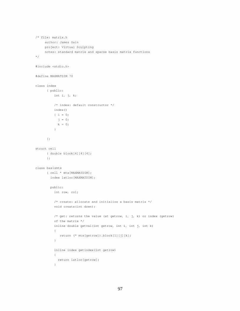
/* file: matrix.h

author: James Gain


notes: standard matrix and sparse basis matrix functions

*/

#include <stdio.h>

#define MAXMATDIM 70

class index

{ public:

int i, j, k;

/* index: default constructor */

index()

{ i = 0;

j = 0;

k = 0;

}

};

struct cell

{ double block[4][4][4];

};

class basismtx

{ cell * mtx[MAXMATDIM];

index latloc[MAXMATDIM];

public:

int row, col;

/* create: allocate and initialize a basis matrix */

void create(int down);

/* get: returns the value (at getrow, i, j, k) or index (getrow)

of the matrix */

inline double getval(int getrow, int i, int j, int k)

{

return (* mtx[getrow]).block[i][j][k];

}

inline index getindex(int getrow)

{

return latloc[getrow];

}

97

/* put: inserts a value or index at position (putrow)

of the matrix */

inline void putval(int putrow, int i, int j, int k, double val)

{

(* mtx[putrow]).block[i][j][k] = val;

}

inline void putindex(int putrow, int li, int lj, int lk)

{

latloc[putrow].i = li;

latloc[putrow].j = lj;

latloc[putrow].k = lk;

}

};

class matrix

{ public:

int row, col;

double * mtx[MAXMATDIM];

/* create: allocate and initialize a matrix */

void create(int down,int across);

/* get: returns the value at position (getrow, getcol) of the matrix */

inline double get(int getrow, int getcol)

{

return ((mtx[getrow])[getcol]);

}

/* put: inserts a value at position (putrow, putcol) of the matrix */

inline void put(int putrow, int putcol, double val)

{

((mtx[putrow])[putcol]) = val;

}

};

98

/* file: vector.h

author: James Gain


notes: Basic vector arithmetic library.

*/

class point

{ public:

double x,y,z;

/* point: default constructor */

point();

};

class vector

{ public:

double i, j, k;

/* vector: default constructor */

vector();

/* (*) scale: scale the vector by a scalar factor c */

friend vector operator *(vector v, double c);

/* (/) divide: divide the first vector by the second */

friend vector operator /(vector a, vector b);

/* (-) difference of points: create a vector from point P to point Q (Q-P) */

friend vector operator -(point p, point q);

/* (+) pnt plus vec: find the point at the head of a vector which

is placed with its tail at p */

friend point operator +(point p, vector v);

};

99

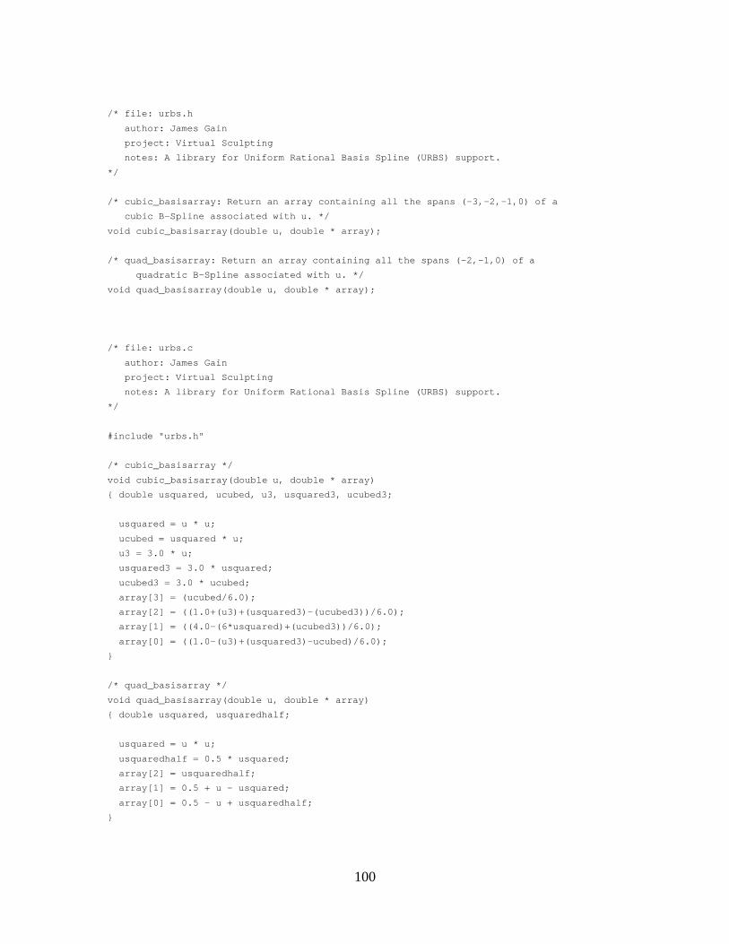
/* file: urbs.h

author: James Gain


notes: A library for Uniform Rational Basis Spline (URBS) support.

*/

/* cubic_basisarray: Return an array containing all the spans (-3,-2,-1,0) of a

cubic B-Spline associated with u. */

void cubic_basisarray(double u, double * array);

/* quad_basisarray: Return an array containing all the spans (-2,-1,0) of a

quadratic B-Spline associated with u. */

void quad_basisarray(double u, double * array);

/* file: urbs.c

author: James Gain


notes: A library for Uniform Rational Basis Spline (URBS) support.

*/

#include "urbs.h"

/* cubic_basisarray */

void cubic_basisarray(double u, double * array)

{ double usquared, ucubed, u3, usquared3, ucubed3;

usquared = u * u;

ucubed = usquared * u;

u3 = 3.0 * u;

usquared3 = 3.0 * usquared;

ucubed3 = 3.0 * ucubed;

array[3] = (ucubed/6.0);

array[2] = ((1.0+(u3)+(usquared3)-(ucubed3))/6.0);

array[1] = ((4.0-(6*usquared)+(ucubed3))/6.0);

array[0] = ((1.0-(u3)+(usquared3)-ucubed)/6.0);

}

/* quad_basisarray */

void quad_basisarray(double u, double * array)

{ double usquared, usquaredhalf;

usquared = u * u;

usquaredhalf = 0.5 * usquared;

array[2] = usquaredhalf;

array[1] = 0.5 + u - usquared;

array[0] = 0.5 - u + usquaredhalf;

}

100

Appendix C

Specification of the RhoVeR System

This appendix describes the Virtual Reality system as designed by the members of the Rhodes Virtual Reality

Special Interest Group. The system consists of a number of processing modules capable of running on a

variety of platforms and contains the communication modules to allow transfer of data between these various

architectures.

This specification details the function of each module and the manner in which interaction between the

modules is expected to occur.

C.1 Overview

Each virtual world will contain a number of instances of various types of modules. Each module consists of

some data associated with a process. Each process is capable of running concurrently with any other process.

The processes communicate using two mechanisms. An event-passing facility allows any process to com-

municate with any other process. A virtual shared memory makes a common data structure available to all

processes.

101

C.2 Interprocess Communication Facilities

C.2.1 Event-passing

All processes are capable of communicating directly with any other process by sending it a message (referred

to in this document as an event). The possible events are predefined. Most processes will contain an event

processing loop which will determine their behaviour when an event of a certain type is received.

C.2.2 The virtual shared memory

The virtual shared memory maintains a data structure which is replicated on all machines used by the virtual

reality system. Only one copy of this replicated database will be maintained per machine, regardless of the

number of modules running on that machine. Any process may read from this data structure. The data

structure contains an entry for every object process (defined later), and only the corresponding object process,

or its parent (defined later), may update that entry. Updates are achieved by sending an update event to the

VSM Manager module on the machine.

C.3 The global data structures

C.3.1 The distributed data base

The data base distributed by the VSM consists of a table containing entries for every module in the virtual

world. Each record in the table consists of the following fields:

� Identifier : This is a unique value for each module in the world.)

� Type of module : Allows object modules to be distinguished so that the relevance of the other fields

can be determined.

� Position : Position of the object in the virtual world.

� Orientation : Orientation of the object in the virtual world.

� Boundary : Border of the object, for collision detection. At present this will be the radius of the

bounding sphere.

� Parent identifier : Identifier of the parent object, equal to its own Identifier if it has no parent.

� Controller identifier: Identifier of the controlling object.

102

� Set of change counters : Give the number of updates to the shape data below to allow processes to

update local copies when these change.

� Generic attributes : attributes which may be useful in various worlds. A fixed number are available

and will be specified as a table containing pairs of values, the attribute identifier (e.g. Mass, Density)

and the attribute value (e.g. 10kg, 5g/m F� �

C.3.2 The shape data

Each object process contains some large tables of data that may be used by other objects. These tables are

not used sufficiently often to justify distributing them everywhere. They will be sent in response to events

requesting them, usually when the requesting process notices a change in the change counter for the table.

The following tables may be found:

� Polygon data : The vertex information for the shape of the object

� Colour : Colour values for the pieces of the object

� Texture : Details of texture maps for pieces of the object

� Generic tables : For temperature and other characteristics of the object

� Device data table : Raw device data for when the object is associated with a particular device

� World attribute list : A list of attributes active in a particular world, usually maintained by the world

module.

� Machine name table : A list of address for all other modules, indexed by the identifier field of the

distributed data base, usually maintained by the world module.

C.3.3 Local values

Each object will contain a tree of its child objects. This will not be shared.

C.4 The modules

The following modules are available. Each module description gives the function of the module and specifies

the manner in which it must respond to events.

All modules share a common event response structure. They will contain the following skeleton:

103

Loop

Event = GetEvent ();

Case Event of

—

—

—

EndCase

EndLoop

Some modules, for example the inputdevice drivers which do not respond to incoming events, can be exempted

from the event polling and evaluation.

At startup, each module must send an event to the world module specifying its address.

C.4.1 The communication modules

C.4.1.1 The Virtual Shared Memory Manager module

The VSM Manager module has one instance per machine. It accepts only update events and discards those

which are from processes that do not have appropriate permission to update the data base. It is responsible

for transmitting the updates to other machines involved in the virtual world system.

The VSM manager responds to two events, an Update from a process wishing to modify its own data, and

an UndergroundUpdate from other VSM managers to transfer approved updates from other machines. The

response to these events is as follows:

Update :

Check if sending process owns the field to be updated

If not, return immediately, no error message is sent

Update local entry

Send UndergroundUpdates to the other VSM Managers

UndergroundUpdate :

Update local entry

The VSM Manager has a role to play at system startup. The world module starts up one VSM Manager per

machine. The VSM Manager must start any other modules local to that machine.

104

C.4.2 The World Control modules

C.4.2.1 The World module

The world module provides centralised control and decides policy for each world. Different worlds will be

completely independent systems whose interaction will be through the corresponding world control modules.

The world modules provides attribute control for the other modules, to regulate a consistent world view. An

attribute list may be retrieved from the world module to set the default behaviour of the object modules.

The world module may also have a role to play in centralised object control, and in access control to the

world. It can also enforce global attributes, such as gravity and collision detection.

The world module maintains a table of addresses for each module in the world. This table is part of the shape

data for the world module.

The world module is involved in system initialization. It is started first and is responsible for starting VSM

Managers on each machine involved in the system. As modules are started up, they report their addresses to

the world module, which must then update its table.

C.4.2.2 The Object modules

The object modules control objects in the virtualworld. Each object is supplied with a standard event-handling

routine which controls the manner in which it responds to incoming events. Only if this routine permits will

the object call a user specified routine to react to the event. In some cases both the user routine and the default

routine will execute.

Objects may be grouped in hierarchies. This hierarchy is a tree structure with the root node referred to as the

parent object. Unless an event is specifically intended for the child process, it will be directed to the parent

object. The parent will then send any relevant information to its children.

Objects are also responsible for maintaining and distributing their shape data on request. This is normally

handled by the default event processing routines.

105

C.4.3 Output Modules

C.4.3.1 Video Output

This renders the world from the viewpoint of a particular object. It may have to query object shape databases

for information needed to draw the object. These queries will only occur if the change counters have changed

in value.

C.4.4 Input Modules

C.4.4.1 Device drivers

These interact with the input devices and transmit their raw data to the object representing the device. For

example, finger positions are transmitted to the hand object.

C.5 Event-passing

Event-passing is handled at a lower level than the sections described previously. The interface to the event

handling routines is handled by two routines:

� Send Event: sends an event of a particular type, together with any required data, to a specified process.

� Get Event: if an event is available, then the type of event, source process and any additional data is

returned, otherwise NULL is returned. The data will be in the correct form for the architecture; any

conversion necessary is performed by the Get Event procedure.

The data component of the event and its data is converted to a standard format (currently that used by Sparc

Solaris 2.2) as part of SendEvent, and converted back to a format suitable for the local processor as part of

GetEvent. Currently this is done on a global basis by exchanging the endian order on groups of 4 bytes.

C.5.1 Send Event

The send event routine will operate as follows:

void SendEvent (Destination, EventType, EventDataSize, EventData)

106

1. If there is no existing connection with the destination process:

(a) Fetch the destination address from the world module.

(b) Open a connection to the destination process.

2. Add the event to the queue of outgoing messages.

3. Attempt to send messages from the queue.

4. Poll incoming connections for events, and add any to the incoming queue.

C.5.2 Get Event and GetMatchingEvent

The GetEvent routine will operate as follows:

1. Check for, and open any new connections to other processes.

2. Poll incoming connections for events, and add any to the incoming queue.

3. Attempt to send messages from the outgoing queue.

4. If there is an event in the incoming queue which matches the required criteria, then return that event.

5. Return NULL.

GetMatchingEvent is intended to allow events to be received out of order, in the special cases where a reply

is required before any further processing can be done. GetEvent uses the same function, but will match the

first available event.

The format conversion occurs just before the events are added to the appropriate queues.

107

Bibliography

[Bangay 1993] Bangay S. (1993) Parallel Implementation of a Virtual

Reality System on a Transputer Architecture. Masters

Thesis, Technical Document PPG 93/10, Rhodes Uni-

versity.

[Barr 1984] Barr A. (1984) Global and Local Deformations of

Solid Primitives. Computer Graphics (Proceedings of

SIGGRAPH ’84), 18(3), pp. 21-30.

[Bartels et al 1987] Bartels R., Beatty J. and Barsky B. (1987) An Intro-

duction to Splines for use in Computer Graphics and

Geometric Modelling. Morgan Kaufmann.

[Bill and Lodha 1994] Bill J. and Lodha S. (1994) Computer Sculpting

of Polygonal Models using Virtual Tools. Technical

Report UCSC-CRL-94-27, University of California,

Santa Cruz.

[Borrel and Bechmann 1992] Borrel P. and Bechmann D. (1991) Deformation of N-

dimensional Objects. International Journal of Compu-

tational Geometry and Applications,1(4), pp. 427-453

[Brijs et al 1993] Brijs P., Hoek, T., Van der Mast C. and Smets G.

Designing in Virtual Reality: Modelling Objects in a

Virtual Environment (MOVE). Technical Report 93-

91, Delft University of Technology.

108

[Burden and Faires 1993] Burden R. and Faires J. (1993) Numerical Analysis

[5th ed]. PWS Publishing Company, Boston.

[Butterworth et al 1992] Butterworth J., Davidson A., Hench S. and Olano T.

(1992) 3DM: A Three Dimensional Modeler Using a

Head-Mounted Display. Proceedings of 1992 Sympo-

sium on Interactive 3D Graphics, ACM SIGGRAPH,

pp. 135-138.

[Celniker and Gossard 1991] Celniker G. and Gossard D. (1991) Deformable Curve

and Surface Finite Elements for Free-Form Shape

Design. Computer Graphics (Proceedings of SIG-

GRAPH ’91), 25(4), pp. 257-266.

[Chadwick et al 1989] Chadwick J., Haumann D. and Parent R. (1989) Lay-

ered Construction for Deformable Animated Charac-

ters. Computer Graphics (Proceedings of SIGGRAPH

’89), 23(3), pp. 243-252.

[Chapin et al 1994] Chapin W., Lacey T. and Leifer L. (1994) De-

signSpace: A Manual Interaction Environment for

Computer Aided Design. Proceedings of CHI ’94, pp.

24-28.

[Coquillart 1987] Coquillart S. (1987) A Control-Point-Based Sweeping

Technique. IEEE Computer Graphics and Applica-

tions, 7(11), pp. 36-45.

[Coquillart 1990] Coquillart S. (1990) Extended Free-Form Deforma-

tion: A Sculpturing Tool for 3D Geometric Model-

ing. Computer Graphics (Proceedings of SIGGRAPH

’90), 24(4), pp. 187-196.

[Coquillart and Jancene 1991] Coquillart S. and Jancene P. (1991) Animated Free-

Form Deformation: An Interactive Animation Tech-

nique. Computer Graphics (Proceedings of SIG-

GRAPH ’91), 25(4), pp. 23-26.

109

[Foley et al 1991] Foley J., Van Dam A., Feiner S. and Hughes J. (1991)

Computer Graphics: Principles and Practice [2nd

ed]. Addison-Wesley Publishing Company.

[Galyean and Hughes 1991] Galyean T. and Hughes J. (1991) Sculpting: An In-

teractive Volumetric Modeling Technique. Computer

Graphics (Proceedings of SIGGRAPH ’92),25(4), pp.

267-274.

[Golub and Van Loan 1989] Golub G. and Van Loan C. (1989) Matrix Computa-

tions [2nd ed]. Johns Hopkins University Press.

[Gourret et al 1989] Gourret J., Magnenat-Thalmann N. and Thalmann D.

(1989) Simulation of Object and Human Skin Defor-

mation in a Grasping Task. Computer Graphics (Pro-

ceedings of SIGGRAPH ’89), 23(3), pp. 21-30.

[Greville 1960] Greville T. (1960) Some Applications of the Pseudoin-

verse of a Matrix. SIAM Review, 2(1), pp. 15-22.

[Hoppe et al 1992] Hoppe H., DeRose T., Duchamp T., McDonald J.

and Stuetzle W. Surface Reconstruction from Unor-

ganized Points. Computer Graphics (Proceedings of

SIGGRAPH ’92), 26(2), pp. 71-78.

[Hsu et al 1992] Hsu W., Hughes J. and Kaufman H. (1992) Direct

Manipulation of Free-Form Deformations. Computer

Graphics (Proceedings of SIGGRAPH ’92),26(2), pp.

177-182.

[Jacobson 1994] Jacobson R. (1994) Virtual Worlds: A New Type of

Design Environment. Virtual Reality World, 2(3), pp.

46-52.

[Johnson et al 1993] Johnson L., Riess R. and Arnold J. (1993) Introduction

to Linear Algebra [3rd ed]. Addison-Wesley Publish-

ing Company.

110

[Latta 1991] Latta J. (1991) When Will Reality Meet the Market-

place? Proceedings of Virtual Reality ’91, Meckler

Publishing, pp. 109-141.

[Lamousin and Waggenspack 1994] Lamousin H. and Waggenspack W. (1994) NURBS-

Based Free-Form Deformation IEEE Computer

Graphics and Applications, 14(6) pp. 59-65.

[Lawson and Hanson 1974] Lawson C. and Hanson R. (1974) Solving Least

Squares Problems. Prentice-Hall, Englewood Cliffs,

NJ.

[Metaxas and Terzopoulos 1992] Metaxas D. and Terzopoulos D. (1992) Dynamic De-

formation of Solid Primitives with Constraints. Com-

puter Graphics (Proceedings of SIGGRAPH ’92),

26(2), pp. 309-312.

[Miller 1986] Miller J. (1986) Sculptured Surfaces in Solid Models:

Issues and Alternative Approaches. IEEE Computer

Graphics and Applications, 6(12), pp. 37-48.

[Nielson 1993] Nielson G. (1993) CAGD’s Top Ten: What to Watch.

IEEE Computer Graphics and Applications, 13(1), pp.

35-37.

[Noble 1969] Noble B. (1969) Applied Linear Algebra. Prentice-

Hall, Englewood Cliffs, NJ.

[Qin and Terzopoulos 1995] Qin H. and Terzopoulos D. (1995) Dynamic Manip-

ulation of Triangular B-Splines. Proceedings of the

Third Symposium on Solid Modeling and Applica-

tions, ACM Press, pp. 351-360.

[Requicha and Rossignac 1992] Requicha A. and Rossignac J. Solid Modeling and

Beyond. IEEE Computer Graphics and Applications,

12(5), pp. 34-44.

[Rheingold 1991] Rheingold H. (1991) Virtual Reality. Summit Books.

111

[Sachs et al 1991] Sachs E., Roberts A. and Stoops D. (1991) 3-Draw:

A Tool for Designing 3D Shapes. IEEE Computer

Graphics and Applications, 11(6), pp. 18-26.

[Schroeder et al 1992] Schroeder W., Zarge J. and Lorensen W. (1992) Deci-

mation of Triangle Meshes. Computer Graphics (Pro-

ceedings of SIGGRAPH ’92), 26(2), pp. 65-70.

[Schumaker 1993] Schumaker L. (1993) Triangulations in CAGD. IEEE

Computer Graphics and Applications, 13(1), pp. 47-

52.

[Sederberg and Parry 1986] Sederberg T. and Parry S. (1986) Free-Form Deforma-

tion of Solid Geometric Models. Computer Graphics

(Proceedings of SIGGRAPH ’86), 20(4), pp. 151-160.

[Shaw and Green 1994] Shaw C. and Green M. (1994) Two-Handed Polygonal

Surface Design. Proceedings of UIST ’94, pp. 205-

212, ACM SIGGRAPH/SIGCHI.

[Shimada and Gossard 1995] Shimada K. and Gossard D. (1995) Bubble Mesh: Au-

tomated Triangular Meshing of Non-Manifold Geom-

etry by Sphere Packing. Proceedings of the Third Sym-

posium on Solid Modeling and Applications, ACM

Press, May, pp. 409-419.

[Stoer and Bulirsch 1983] Stoer J. and Bulirsch R. (1983) Introduction to Nu-

merical Analysis. Springer-Verlag, New York.

[Terzopoulos and Fleischer 1988] Terzopoulos D. and Fleischer K. (1988) Modeling In-

elastic Deformation: Viscoelasticity, Plasticity, Frac-

ture. Computer Graphics (Proceedings of SIGGRAPH

’88), 22(4), pp. 269-278.

[Welch and Witkins 1992] Welch W. and Witkins A. (1992) Variational Surface

Modeling. Computer Graphics (Proceedings of SIG-

GRAPH ’92), 26(2), pp. 157-165.

112

[Welch and Witkins 1994] Welch W. and Witkins A. (1994) Free-Form Shape De-

sign using Triangulated Surfaces. Computer Graphics

(Proceedings of SIGGRAPH ’94), pp. 247-256.

[Wordenweber 1983] Wordenweber B. (1983) Surface Triangulation for

Picture Production. IEEE Computer Graphics and

Applications, 3(8), pp. 45-51.

113

virtual sculpting: an investigation of directly manipulated free … · b directly manipulated...

Documents