Visibility in Computer Graphics

Jirı Bittner†§ and Peter Wonka§‡

†Center for Applied CyberneticsCzech Technical University in Prague

§Institute of Computer Graphics and AlgorithmsVienna University of Technology

‡Graphics, Visualization, and Usability CenterGeorgia Institute of Technology

Abstract

Visibility computation is crucial for computer graphicsfrom its very beginning. The first visibility algorithmsin computer graphics aimed to determine visible sur-faces in a synthesized image of a 3D scene. Nowa-days there are many different visibility algorithms forvarious visibility problems. We propose a new taxon-omy of visibility problems that is based on a classifi-cation according to the problem domain. We providea broad overview of visibility problems and algorithmsin computer graphics grouped by the proposed taxon-omy. The paper surveys visible surface algorithms,visibility culling algorithms, visibility algorithms forshadow computation, global illumination, point-basedand image-based rendering, and global visibility com-putations. Finally, we discuss common concepts of vis-ibility algorithm design and several criteria for the clas-sification of visibility algorithms.

1 Introduction

Visibility is studied in computer graphics, architecture,computational geometry, computer vision, robotics,telecommunications, and other research areas. In thispaper we discuss visibility problems and algorithmsfrom the point of view of computer graphics.

Computer graphics aims to synthesize images of vir-tual scenes by simulating the propagation of light. Visi-bility is a crucial phenomenon that is an integral part ofthe interaction of light with the environment. The firstvisibility algorithms aimed to determine which lines

or surfaces are visible in a synthesized image of a 3Dscene. These problems are known asvisible line andvisible surfacedetermination or ashidden lineandhid-den surfaceremoval. The classical visible line and visi-ble surface algorithms were developed in the early daysof computer graphics in the late 60’s and the begin-ning of the 70’s (Sutherlandet al., 1974). These tech-niques were mostly designed for vector displays. Later,with increasing availability of raster devices the tradi-tional techniques were replaced by the z-buffer algo-rithm (Catmull, 1975). Nowadays, we can identify twowidely spread visibility algorithms: the z-buffer for vis-ible surface determination and ray shooting for comput-ing visibility along a single ray. The z-buffer and itsmodifications dominate the area of real-time renderingwhereas ray shooting is commonly used in the scopeof global illumination methods. Besides these two ele-mentary methods there is a plethora of visibility algo-rithms for various specific visibility problems.

Several surveys of visibility methods have been pub-lished. The classical survey of Sutherland, Sproull,and Schumacker (1974) covers ten traditional visi-ble surface algorithms. This survey was updated byGrant (1992) who provides a classification of visibil-ity algorithms that includes newer rendering paradigmssuch as distributed ray tracing. A survey of Du-rand (1999) provides a comprehensive multidisci-plinary overview of visibility techniques in various re-search areas. A recent survey of Cohen-Or et al. (2002)summarizes visibility algorithms for walkthrough ap-plications.

In this paper we aim to provide a new taxonomy ofvisibility problems encountered in computer graphics

1

based on the problem domain. The taxonomy shouldhelp to understand the nature of a particular visibilityproblem and provides a tool for grouping problems ofsimilar complexity independently of their target appli-cation. We provide a broad overview of visibility prob-lems and algorithms in computer graphics grouped bythe proposed taxonomy. The paper surveys visible sur-face algorithms, visibility culling algorithms for, visi-bility algorithms for shadow computation, global illu-mination, point-based and image-based rendering, andglobal visibility computations.

In contrast to the previous surveys, we focus onthe common ideas and concepts rather than algorith-mic details. We aim to assist a potential algorithmdesigner in transferring the concepts developed in thecomputer graphics community to solve visibility prob-lems in other research areas.

2 Taxonomy of visibility problems

Visibility is a phenomenon that can be defined by meansof mutually unoccluded points: two points are mutu-ally visible if the line segment connecting them is un-occluded. From this definition we can make two obser-vations: (1) lines carry visibility, (2) two points can bevisible regardless of their distance.

The first observation says that the domain of a visibil-ity problem is formed by the set of lines through whichthe scene entities might be visible. We call this set theproblem-relevant line set. The second observation saysthat visibility of scene entities is independent of theirspatial proximity.

2.1 Problem domain

The problem domain is given by the problem-relevantline set, i.e. by the set of lines involved in the solutionof the problem. Computer graphics deals with the fol-lowing domains:

1. visibility along a line

2. visibility from a point

3. visibility from a line segment

4. visibility from a polygon

5. visibility from a region

6. global visibility

The domain description is independent of the dimen-sion of the scene, i.e. the problem of visibility from apoint can be stated for 2D, 212D, and 3D scenes. Theactual domains however differ depending on the scenedimension. For example, as we shall see later, visibilityfrom a polygon is equivalent to visibility from a regionin 2D, but not in 3D.

The problem domains can further be categorized asdiscrete or continuous. A discrete domain consists of afinite set of lines (rays), which is a common situationwhen the problem aims at computing visibility with re-spect to a raster image.

2.1.1 The dimension of visibility problems

We assume that a line inprimal spacecan be mappedto a point inline space(Stolfi, 1991; Pellegrini, 1997;Teller, 1992b; Durand, 1999). In 3D there are four de-grees of freedom in the description of a line and thus thecorresponding line space is four-dimensional. Fixingcertain line parameters (e.g. direction), the problem-relevant line set, denotedL3

x, forms ak-dimensionalsubset ofR4, where0 ≤ k ≤ 4. The superscript (3)expresses the dimension of primal space, the subscript(x) corresponds to one of the problem domain classes:lfor visibility along a line,p for visibility from a point,sfor visibility from a line segment,n for visibility from apolygon,r for visibility from a region, andg for globalvisibility.

In 2D there are two degrees of freedom in the de-scription of a line and the corresponding line spaceis two-dimensional. Therefore, the problem-relevantline setL2

x forms ak-dimensional subset ofR2, where0 ≤ k ≤ 2. An illustration of the concept of theproblem-relevant line set is depicted in Figure 1.

For the purpose of this discussion we define the di-mension of the visibility problem as the dimension ofthe corresponding problem-relevant line set.

2.2 Visibility along a line

The simplest visibility problems deal with visibilityalong a single line. The problem-relevant line set iszero-dimensional, i.e. it is fully specified by the givenline. The visibility along a line problems can be solvedby computing intersections of the given line with thescene objects.

The most common visibility along a line problem isray shooting(Arvo & Kirk, 1989). Given a ray, rayshooting determines the first intersection of the ray with

2

visibility visibility visibilityfrom a point from a segmentalong a line

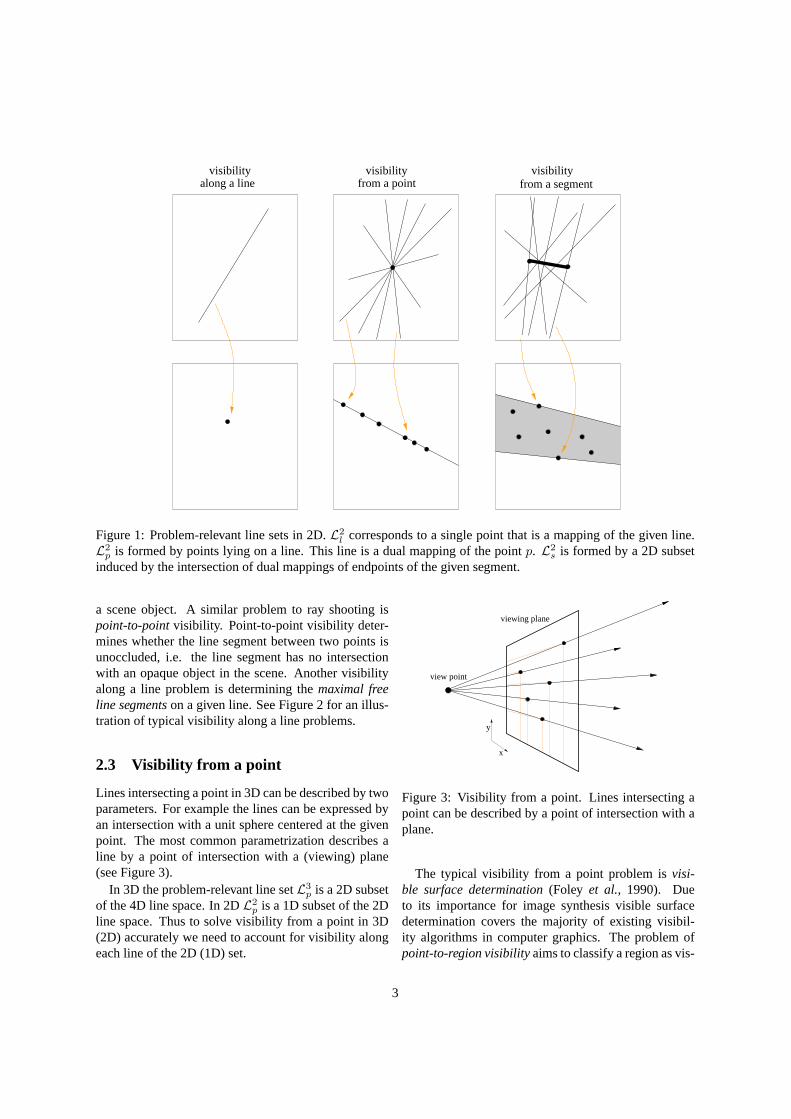
Figure 1: Problem-relevant line sets in 2D.L2l corresponds to a single point that is a mapping of the given line.

L2p is formed by points lying on a line. This line is a dual mapping of the pointp. L2

s is formed by a 2D subsetinduced by the intersection of dual mappings of endpoints of the given segment.

a scene object. A similar problem to ray shooting ispoint-to-pointvisibility. Point-to-point visibility deter-mines whether the line segment between two points isunoccluded, i.e. the line segment has no intersectionwith an opaque object in the scene. Another visibilityalong a line problem is determining themaximal freeline segmentson a given line. See Figure 2 for an illus-tration of typical visibility along a line problems.

2.3 Visibility from a point

Lines intersecting a point in 3D can be described by twoparameters. For example the lines can be expressed byan intersection with a unit sphere centered at the givenpoint. The most common parametrization describes aline by a point of intersection with a (viewing) plane(see Figure 3).

In 3D the problem-relevant line setL3p is a 2D subset

of the 4D line space. In 2DL2p is a 1D subset of the 2D

line space. Thus to solve visibility from a point in 3D(2D) accurately we need to account for visibility alongeach line of the 2D (1D) set.

x

y

viewing plane

view point

Figure 3: Visibility from a point. Lines intersecting apoint can be described by a point of intersection with aplane.

The typical visibility from a point problem isvisi-ble surface determination(Foley et al., 1990). Dueto its importance for image synthesis visible surfacedetermination covers the majority of existing visibil-ity algorithms in computer graphics. The problem ofpoint-to-region visibilityaims to classify a region as vis-

3

A A

B

invisible

A

B

Figure 2: Visibility along a line. (left) Ray shooting. (center) Point-to-point visibility. (right) Maximal free linesegments between two points.

ible, invisible, or partially visible with respect to thegiven point (Teller & Sequin, 1991). Another visibilityfrom a point problem is the construction of thevisibilitymap(Stewart & Karkanis, 1998), i.e. a graph describingthe given view of the scene including its topology.

2.4 Visibility from a line segment

Lines intersecting a line segment in 3D can be describedby three parameters. One parameter fixes the inter-section of the line with the segment the other two ex-press the direction of the line. Thus we can imageLx

s

as a 1D set ofLxp that are associated with all points

on the given segment (see Figure 4). The problem-relevant line setL3

s is three-dimensional andL2s is two-

dimensional. An interesting observation is that in 2D,visibility from a line segment already reaches the di-mension of the whole line space.

L0

0.5L

L0

0.5L

L1L1

1

0.5

0

0 0.5 1

line spacesegment

y

xx

y

u

u

object

planeoccluded

lines

Figure 4: Visibility from a line segment. Lines inter-secting a line segment formL3

s. The figure shows apossible parametrization that stacks up 2D planes. Eachplane corresponds to mappings of lines intersecting apoint on the given line segment.

Thesegment-to-region visibility(Wonkaet al., 2000)is used for visibility preprocessing in 212D scenes. Visi-bility from a line segment also arises in the computationof soft shadows due to a linear light source (Heidrichet al., 2000).

2.5 Visibility from a polygon

In 3D, lines intersecting a polygon can be described byfour parameters (Guet al., 1997; Pellegrini, 1997). Forexample: two parameters fix a point inside the poly-gon, the other two parameters describe a direction ofthe line. We can imagineL3

n as a 2D set ofL3p associ-

ated with all points inside the polygon (see Figure 4).L3

n is a four-dimensional subset of the 4D line space.In 2D, lines intersecting a polygon consists of sets thatintersect the boundary line segments of the polygon andthusL2

n is two-dimensional. Visibility from a poly-gon problems include computing a form-factor betweentwo polygons (Goralet al., 1984), soft shadow algo-rithms (Chin & Feiner, 1992), and discontinuity mesh-ing (Heckbert, 1992).

2.6 Visibility from a region

Lines intersecting a volumetric region in 3D can be de-scribed by four parameters. Similarly to the case oflines intersecting a polygon two parameters can fix apoint on the boundary of the region, the other two fixthe direction of the line. ThusL3

r is four-dimensionaland the corresponding visibility problems belong to thesame complexity class as the from-polygon visibilityproblems. In 2D, visibility from a 2D region is equiv-alent to visibility from a polygon:L2

r is a 2D subset of2D line space.

4

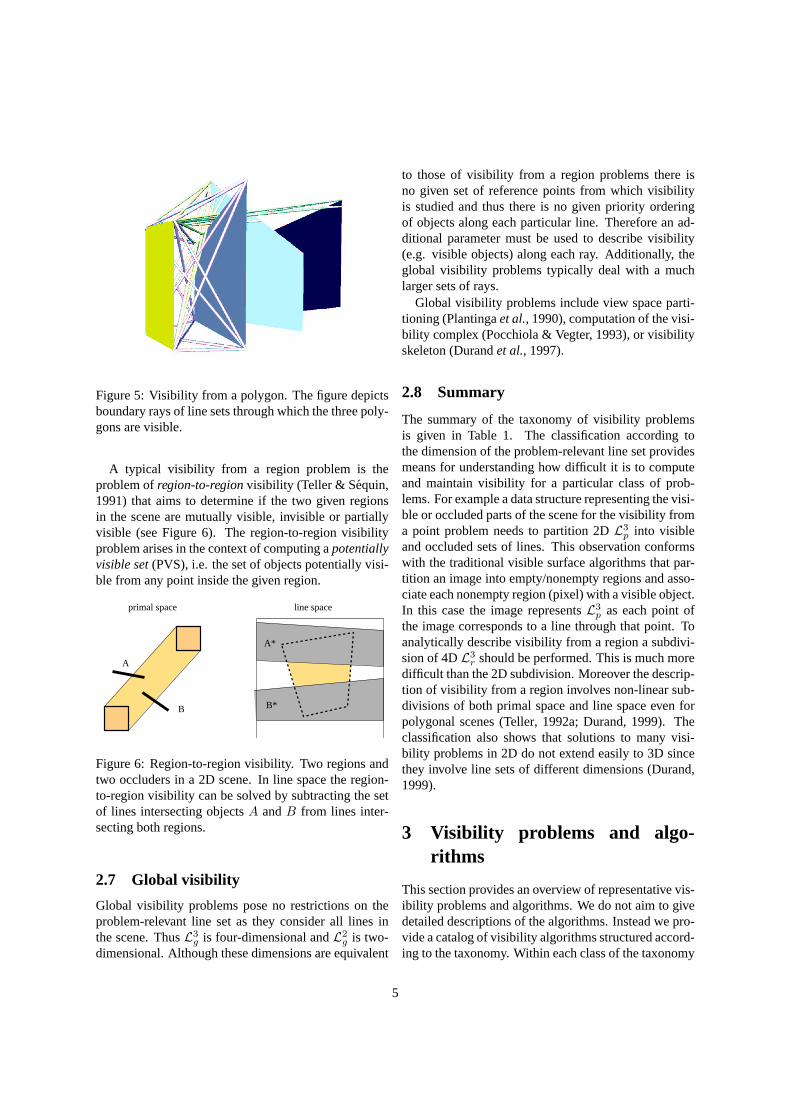
Figure 5: Visibility from a polygon. The figure depictsboundary rays of line sets through which the three poly-gons are visible.

A typical visibility from a region problem is theproblem ofregion-to-regionvisibility (Teller & Sequin,1991) that aims to determine if the two given regionsin the scene are mutually visible, invisible or partiallyvisible (see Figure 6). The region-to-region visibilityproblem arises in the context of computing apotentiallyvisible set(PVS), i.e. the set of objects potentially visi-ble from any point inside the given region.

primal space line space

B

A

B*

A*

Figure 6: Region-to-region visibility. Two regions andtwo occluders in a 2D scene. In line space the region-to-region visibility can be solved by subtracting the setof lines intersecting objectsA andB from lines inter-secting both regions.

2.7 Global visibility

Global visibility problems pose no restrictions on theproblem-relevant line set as they consider all lines inthe scene. ThusL3

g is four-dimensional andL2g is two-

dimensional. Although these dimensions are equivalent

to those of visibility from a region problems there isno given set of reference points from which visibilityis studied and thus there is no given priority orderingof objects along each particular line. Therefore an ad-ditional parameter must be used to describe visibility(e.g. visible objects) along each ray. Additionally, theglobal visibility problems typically deal with a muchlarger sets of rays.

Global visibility problems include view space parti-tioning (Plantingaet al., 1990), computation of the visi-bility complex (Pocchiola & Vegter, 1993), or visibilityskeleton (Durandet al., 1997).

2.8 Summary

The summary of the taxonomy of visibility problemsis given in Table 1. The classification according tothe dimension of the problem-relevant line set providesmeans for understanding how difficult it is to computeand maintain visibility for a particular class of prob-lems. For example a data structure representing the visi-ble or occluded parts of the scene for the visibility froma point problem needs to partition 2DL3

p into visibleand occluded sets of lines. This observation conformswith the traditional visible surface algorithms that par-tition an image into empty/nonempty regions and asso-ciate each nonempty region (pixel) with a visible object.In this case the image representsL3

p as each point ofthe image corresponds to a line through that point. Toanalytically describe visibility from a region a subdivi-sion of 4DL3

r should be performed. This is much moredifficult than the 2D subdivision. Moreover the descrip-tion of visibility from a region involves non-linear sub-divisions of both primal space and line space even forpolygonal scenes (Teller, 1992a; Durand, 1999). Theclassification also shows that solutions to many visi-bility problems in 2D do not extend easily to 3D sincethey involve line sets of different dimensions (Durand,1999).

3 Visibility problems and algo-rithms

This section provides an overview of representative vis-ibility problems and algorithms. We do not aim to givedetailed descriptions of the algorithms. Instead we pro-vide a catalog of visibility algorithms structured accord-ing to the taxonomy. Within each class of the taxonomy

5

problem dimension of commondomain Ly

x problems

2D

visibility along a line 0ray shootingpoint-to-point visibility

visibility from a point 1view around a pointpoint-to-region visibility

visibility from a line segment

2region-to-region visibilityPVS

visibility from a polygonvisibility from a regionglobal visibility

3D

visibility along a line 0ray shootingpoint-to-point visibility

visibility from a point 2

visible (hidden) surfacespoint-to-region visibilityvisibility maphard shadows

visibility from a line segment 3segment-to-region visibilitysoft shadowsPVS in 21

2D scenes

visibility from a polygonvisibility from a regionglobal visibility

4

region-to-region visibilityPVSaspect graphsoft shadowsdiscontinuity meshing

Table 1: Classification of visibility problems according to the dimension of the problem-relevant line set.

the algorithms are grouped according to the actual visi-bility problem or important algorithmic features.

3.1 Visibility along a line

Ray shooting Ray shooting is the most common vis-ibility along a line problem. Given a ray, ray shootingdetermines the first intersection of the ray with a sceneobject. Ray shooting was first used by Appel (1968) tosolve the visible surface problem for each pixel of theimage. Ray shooting is the core of theray tracingalgo-rithm (Whitted, 1979) that follows light paths from theview point backwards to the scene. Many recent meth-ods use ray shooting driven by stochastic sampling formore accurate simulation of light propagation (Kajiya,1986; Arvo & Kirk, 1990). A naive ray shooting algo-rithm tests all objects for intersection with a given rayto find the closest visible object along the ray inΘ(n)time (wheren is the number of objects). For complexscenes even the linear time complexity is very restric-tive since a huge amount of rays is needed to synthesizean image. An overview of acceleration techniques forray shooting was given by Arvo (1989). A recent survey

was presented by Havran (2000).

Point-to-point visibility Point-to-point visibility isused within the ray tracing algorithm (Whitted, 1979) totest whether a given point is in shadow with respect toa point light source. This query is typically resolved bycasting shadow rays from the given point towards thelight source. This process can be accelerated by pre-processing visibility from the light source (Haines &Greenberg, 1986; Woo & Amanatides, 1990) (see Sec-tion 3.2.5 for more details).

3.2 Visibility from a point

Visibility from a point problems cover the majority ofvisibility algorithms developed in the computer graph-ics community. We subdivide this section according tofive subclasses: visible surface determination, visibilityculling, hard shadows, global illumination, and image-based and point-based rendering.

6

3.2.1 Visible surface determination

Visible surface determination aims to determine visiblesurfaces in the synthesized image, which is the mostcommon visibility problem in computer graphics.

Z-buffer The z-buffer, introduced by Catmull (1975),is one of the simplest visible surface algorithms. Itssimplicity allows an efficient hardware implementationand therefore the z-buffer is nowadays commonly avail-able even on low cost graphics hardware. The z-bufferis a discrete algorithm that associates a depth value witheach pixel of the image. The z-buffer performs discretesampling of visibility and therefore the rendering algo-rithms based on the z-buffer are prone to aliasing (Car-penter, 1984).

The z-buffer algorithm is notoutput sensitivesince itneeds to rasterize all scene objects even if many objectsare invisible. This is not restrictive for scenes wheremost of the scene elements are visible, such as a singlealbeit complex object. For large scenes with high depthcomplexity the processing of invisible objects causessignificantoverdraw. Overdraw expresses how manypolygons are rasterized at a pixel (only the closest poly-gon is actually visible). The overdraw problem is ad-dressed by visibility culling methods that will be dis-cussed in Section 3.2.4.

List priority algorithms List priority algorithms de-termine an ordering of scene objects so that a correctimage is produced if the objects are rendered in this or-der. Typically objects are processed in back-to-front or-der: closer objects are painted over the farther ones inthe frame buffer. In some cases no suitable order ex-ists due to cyclic overlaps and therefore some object(s)have to be split. The list priority algorithms differ ac-cording to which objects get split and when the splittingoccurs (Foleyet al., 1990). Thedepth sort algorithmby Newell et al. (1972) renders polygons in the framebuffer in the order of decreasing distance from the viewpoint. This is performed by partial sorting of poly-gons according to their depths and resolving possibledepth overlaps. A simplified variant of this algorithmthat ignores the overlap checks is called thepainter’salgorithm due to the similarity to the way a paintermight paint closer objects over distant ones. Thebinaryspace partitioning(BSP) tree introduced by Fuchs, Ke-dem, and Naylor (1980) allows the efficient calculationof visibility ordering among static polygons in a scene

seen from an arbitrary view point. Improved output-sensitive variants of the algorithm generate a front-to-back order of polygons and an image space data struc-ture for correct image updates (Gordon & Chen, 1991;Naylor, 1992).

Area subdivision algorithms Warnock (1969) devel-oped an area subdivision algorithm that subdivides agiven image area into four rectangles. In the case thatvisibility within the current rectangle cannot be solved,the rectangle is recursively subdivided. The subdivisionis terminated when the area matches the pixel size. Thealgorithm of Weiler and Atherton (1977) subdivides theimage plane using the actual polygon boundaries. Thealgorithm does not rely on a pixel resolution but it re-quires a robust polygon clipping algorithm.

Scan line algorithms The scan-line visibility algo-rithms extend the scan conversion of a single poly-gon (Foleyet al., 1990). They maintain an active edgetable that indicates which polygons span the currentscan line. The scan line coherence is exploited usingincremental updates of the active edge table similarlyto the scan conversion of a single polygon.

Ray casting Ray casting (Appel, 1968) is a visiblesurface algorithm that solves visibility by ray shooting.More specifically by shooting rays through each pixelin the image. The advantage of ray casting is that it isinherently output sensitive (Waldet al., 2001).

3.2.2 Visibility maps

A visibility map is a graph describing a view of thescene including its topology. Stewart and Karka-nis (1998) proposed an algorithm for the constructionof approximate visibility maps using dedicated graphicshardware. They use an item buffer and graph relaxationto determine edges and vertices of visible scene poly-gons and their topology. Grasset et al. (1999) dealt withsome theoretical operations on visibility maps and theirapplications in computer graphics. Bittner (2002a) usesa BSP tree to calculate and represent the visibility map.

3.2.3 Back face culling and view frustum culling

Back face culling aims to avoid rendering of polygonsthat are not facing the view point. View frustum cullingeliminates polygons that do not intersect the viewing

7

frustum. These two methods are heavily exploited inreal-time rendering applications. Both techniques pro-vide simple decisions, but they do not account for oc-clusion. See Moller and Haines (1999) for a detaileddiscussion.

3.2.4 Visibility culling

Visibility culling algorithms aim to accelerate renderingof large scenes by quickly culling invisible parts of thescene. The final hidden surface removal is typically car-ried out using the z-buffer. To avoid image artifacts vis-ibility culling algorithms are usuallyconservative, i.e.,they never classify a visible object as invisible. In real-time rendering applications the scene usually consistsof a large set of triangles. Due to efficiency reasons it iscommon to calculate visibility for a group of trianglesrather than for each triangle separately.

General scenes The z-buffer is a basic and robust toolfor hidden surface removal, but it can be very inefficientfor scenes with a high depth-complexity. This problemis addressed by thehierarchical z-bufferalgorithm de-veloped by Greene et al. (1993). The hierarchical z-buffer uses a z-pyramid to represent image depths andan octree to organize the scene. The z-pyramid is usedto test visibility of octree bounding boxes. Zhang etal. (1997) proposed an algorithm that replaces the z-pyramid by ahierarchical occlusion mapand adepthestimation buffer. This approach was further studied byAila (2000).

Newer graphics hardware provides an occlusion testfor bounding boxes (e.g. ATI, NVIDIA). The problemof this occlusion test is that the result of such an oc-clusion query is not readily available. A straightfor-ward algorithm would therefore cause many unneces-sary delays (pipeline stalls) in the rendering. The focusof research has now shifted to finding ways of order-ing the scene traversal to interleave rendering and vis-ibility queries in an efficient manner (Heyet al., 2001;Klosowski & Silva., 2001).

Scenes with large occluders Another class of algo-rithms selects several large occluders and performs vis-ibility culling in object space. Hudson (1997) usesshadow volumes of each selected occluder indepen-dently to check visibility of a spatial hierarchy. Coorgand Teller (1997) track visibility from the view pointby maintaining a set of planes corresponding to visibil-

ity changes. Bittner et al. (1998) construct an occlusiontree that merges occlusion volumes of the selected oc-cluders.

Urban scenes Visibility algorithms for indoor scenesuse a natural partitioning of architectural scenes intocells and portals. Cells correspond to rooms and portalscorrespond to doors and windows (Aireyet al., 1990).Luebke and Georges (1995) proposed a simple conser-vative cell/portal visibility algorithm for indoor scenes.

Wonka and Schmalstieg (1999) used occluder shad-ows and the z-buffer for visibility culling in 212D scenesand Downs et al. (2001) use occlusion horizons main-tained by a binary tree for the same class of scenes.

Terrains Terrain visibility algorithms developed inthe GIS and the computational geometry communi-ties are surveyed by De Floriani and Magillo (1995).In computer graphics, Cohen-Or et al. (1995) pro-posed an algorithm that reduces a visibility from apoint problem in 212D to a series of problems in 112D.Lee and Shin (1997) use vertical ray coherence to ac-celerate rendering of a digital elevation map. Lloydand Egbert (2002) use an adaption of occlusion hori-zons (Downset al., 2001) to calculate visibility for ter-rains.

3.2.5 Hard shadows

The presence of shadows in a computer generated im-age significantly increases its realism. Shadows provideimportant visual cues about position and size of an ob-ject in the scene. A shadow due to a point light sourceand an object is the volume from which the light sourceis hidden by the object. We discuss several importantalgorithms for computing hard shadows. A detaileddiscussion of shadow algorithms can be found in (Wooet al., 1990) and (Moller & Haines, 1999).

Ray tracing Ray tracing (Whitted, 1979) does not ex-plicitly reconstruct shadow volumes. Instead it samplespoints on surfaces using a point-to-point visibility query(see Section 2.2) to test if the points are in shadow.Tracing of shadow rays can be significantly acceleratedby using a light buffer introduced by Haines and Green-berg (1986). The light buffer is a 2D array that asso-ciates with each entry a list of objects intersected by thecorresponding rays. Woo and Amanatides (1990) pro-posed to precompute shadowed regions with respect to

8

the light source and store this information within thespatial subdivision.

Shadow maps Shadow maps proposed byWilliams (1978) provide a discrete representationof shadows due to a single point light source. A shadowmap is a 2D image of the scene as seen from the lightsource. Each pixel of the image contains the depth ofthe closest object to the light source. The algorithmconstructs a shadow map by rendering the scene into az-buffer using the light source as the view point. Thenthe scene is rendered using a given view and visiblepoints are projected into the shadow map. The depthvalue of a point is compared to the value stored in theshadow map. If the point is farther than the storedvalue it is in shadow. This algorithm can be acceleratedusing graphics hardware (Segalet al., 1992). Shadowmaps can represent shadow due to objects definedby complex surfaces, i.e. any object that can berasterized into the shadow map is suitable. In contrastto ray tracing the shadow map approach explicitlyreconstructs the shadow volume and represents it in adiscrete form. Several techniques have been proposedto reduce the aliasing due to the discretization (Grant,1992; Stamminger & Drettakis, 2002).

Shadow volumes The shadow volume of a polygonwith respect to a point is a semi infinite frustum. Theintersection of the frustum with the scene boundingvolume can be explicitly reconstructed and representedby a set of shadow polygons bounding the frustum.Crow (1977) proposed that these polygons can be usedto test if a point corresponding to the pixel of therendered image is in shadow by counting the numberof shadow polygons in front of and behind the point.Heidmann (1991) proposed an efficient real-time im-plementation of the shadow volume algorithm. Theshadow volume BSP(SVBSP) tree proposed by Chinand Feiner (1989) provides an efficient representationof a union of shadow volumes of a set of convex poly-gons. The SVBSP tree is used to explicitly compute litand shadowed fragments of scene polygons. An adapta-tion of the SVBSP method to dynamic scenes was stud-ied by Chrysanthou and Slater (1995). See Figure 7 foran illustration of the output of the SVBSP algorithm.

light source

Figure 7: A mesh resulting from subdividing the sceneusing a SVBSP tree. The darker patches are invisiblefrom the light source.

3.2.6 Global illumination

Beam tracing The beam tracingdesigned by Heck-bert and Hanrahan (1984) casts a pyramid (beam) ofrays rather than shooting a single ray at a time. The re-sulting algorithm makes use of ray coherence and elim-inates some aliasing connected with the classical raytracing.

Cone tracing The cone tracingproposed by Ama-natides (1984) traces a cone of rays at a time insteadof a polyhedral beam or a single ray. In contrast to thebeam tracing the algorithm does not determine preciseboundaries of visibility changes. The cones are inter-sected with the scene objects and at each intersected ob-ject a new cone (or cones) is cast to simulate reflectionand refraction.

Bundle tracing Most stochastic global illuminationmethods shoot rays independently and thus they do notexploit visibility coherence among rays. An excep-tion is theray bundle tracingintroduced by Szirmay-Kalos (1998) that shoots a set of parallel rays throughthe scene according to a randomly sampled direction.This approach allows to exploit ray coherence by trac-ing many rays at the same time.

3.2.7 Image-based and Point-based rendering

Image-based and point-based rendering generate im-ages from point-sampled representations like images or

9

point clouds. This is useful for highly complex mod-els, which would otherwise require a huge number oftriangles. A point is infinitely small by definition andso the visibility of the point samples is determined us-ing a local reconstruction of the sampled surface that isinherent in the particular rendering algorithm.

Image warping McMillan (1997) proposed an algo-rithm for warping images from one view point to an-other. The algorithm resolves visibility by a correct oc-clusion compatible traversal of the input image withoutusing additional data structures like a z-buffer.

Splatting Most point-based rendering algorithmsproject points on the screen usingsplatting. Splattingis used to avoid gaps in the image and to resolve visibil-ity of projected points. Pfister et al. (2000) use soft-ware visibility splatting. Rusinkiewicz et al. (2000)use a hardware accelerated z-buffer and Grossman andDally (1998) use the hierarchical z-buffer (Greeneet al.,1993) to resolve visibility.

Random sampling The randomized z-bufferalgo-rithm proposed by Wand et al. (2001) culls triangles un-der the assumption that many small triangles project toa single pixel. A large triangle mesh is sampled and vis-ibility of the samples is resolved using the z-buffer. Thealgorithm selects a sufficient number of sample pointsso that each pixel receives a sample from a visible tri-angle with high probability.

3.3 Visibility from a line segment

We discuss visibility from a line segment in the scopeof visibility culling and computing soft shadows.

3.3.1 Visibility culling

Several algorithms calculate visibility in 212D urban en-vironments for a region of space using a series of visi-bility from a line segment queries. The PVS for a givenview cell is a union of PVSs computed for all ’top-edges’ of the viewing region (Wonkaet al., 2000).

Wonka et al. (2000) use occluder shrinking and pointsampling to calculate visibility with the help of a hard-ware accelerated z-buffer. Koltun et al. (2001) trans-form the 212D problem to a series of 2D visibility prob-lems. The 2D problems are solved using dual ray spaceand the z-buffer algorithm. Bittner et al. (2001) use a

line space subdivision maintained by a BSP tree to cal-culate the PVS. Figure 8 illustrates the concept of a PVSin a 21

2D scene.

3.3.2 Soft shadows

Heidrich et al. (2000) proposed an extension of theshadow map approach forlinear light sources (line seg-ments). They use a discrete shadow map enriched bya visibility channelto render soft shadows at interac-tive speeds. The visibility channel stores the percentageof the light source that is visible at the correspondingpoint.

3.4 Visibility from a polygon

Visibility from a polygon problems are commonly stud-ied by realistic rendering algorithms that aim to captureillumination due to areal light sources. We discuss thefollowing problems: computing soft shadows, evaluat-ing form factors, and discontinuity meshing.

3.4.1 Soft shadows

Soft shadows appear in scenes with areal light sources.A shadow due to an areal light source consists of twoparts: umbraandpenumbra. Umbra is the part of theshadow from which the light source is completely invis-ible. Penumbra is the part from which the light sourceis partially visible and partially hidden by some sceneobjects. The rendering of soft shadows is significantlymore difficult than rendering of hard shadows mainlydue to complex visibility interactions in penumbra.

Ray tracing A straightforward extension of the raytracing algorithm handles areal light sources by shoot-ing randomly distributed shadow rays towards the lightsource (Cooket al., 1984).

Shadow volumes An adaptation of the SVBSP treefor areal light sources was proposed by Chin andFeiner (1992). Chrysanthou and Slater (1997) useda shadow overlap cube to accelerate updates of softshadows in dynamic polygonal scenes. For each poly-gon they maintain an approximate discontinuity meshto accurately capture shadow boundaries (discontinuitymeshing will be discussed in the next section).

10

(a) (b) (c)

Figure 8: A PVS in a 212D scene representing 8 km2 of Vienna. (a) A selected view cell and the correspondingPVS. The dark regions were culled by hierarchical visibility tests. (b) A closeup of the view cell and its PVS. (c)A snapshot of an observer’s view from a view point inside the view cell.

Shadow textures Heckbert and Herf (1997) proposedan algorithm constructing a shadow texture for eachscene polygon. The texture is created by smoothed pro-jections of the scene from multiple sample points on thelight source. Soler and Sillion (1998) calculate shadowtextures using convolution of the ’point-light shadowmap’ and an image representing the areal light source.

3.4.2 Form-factors

Form-factorsare used in radiosity (Goralet al., 1984)global illumination algorithms. A form-factor ex-presses the mutual transfer of energy between twopatches in the scene. Resolving visibility between thepatches is crucial for the form-factor computation.

Hemi-cube The hemi-cubealgorithm proposed byCohen and Greenberg (1985) computes a form-factorof a differential area with respect to all patches in thescene. The form-factor between the two patches is es-timated by solving visibility at the middle of the patchassuming that the form-factor is almost constant acrossthe patch. Thus the hemi-cube algorithm approximatesa visibility from a polygon problem by solving a visi-bility from a point problem. There are two sources oferrors in the hemi-cube algorithm: the finite resolutionof the hemi-cube and the fact that visibility is sampledonly at one point on the patch.

Ray shooting Wallace et al. (1989) proposed a pro-gressive radiosity algorithm that samples visibility by

ray shooting. Campbell and Fussell (1990) extend thismethod by using a shadow volume BSP tree to resolvevisibility.

Discontinuity meshing Discontinuity meshing wasintroduced by Heckbert (1992) and Lischinski etal. (1992). A discontinuity mesh partitions scene poly-gons into patches so that each patch ’sees’ a topologi-cally equivalent view of the light source. Boundaries ofthe mesh correspond to loci of discontinuities in the illu-mination function. The algorithms of Heckbert (1992)and Lischinski et al. (1992) construct a subset of the dis-continuity mesh by casting planes corresponding to thevertex-edgevisibility events. More elaborated methodscapable of creating a complete discontinuity mesh wereintroduced by Drettakis and Fiume (1994) and Stew-art and Ghali (1994). Discontinuity meshing can beused for computing accurate soft shadows or to ana-lytically calculate form-factors with respect to an areallight source.

3.5 Visibility from a region

Visibility from a region problems arise in the contextof visibility preprocessing. According to our taxonomythe complexity of the from-polygon and from-regionvisibility in 3D is identical. In fact most visibility froma region algorithms solve the problem by computing aseries of from-polygon visibility queries.

11

3.5.1 Visibility culling

An offline visibility culling algorithm calculates a PVSof objects that are potentially visible from any point in-side a given viewing region.

General scenes Durand et al. (2000) proposed ex-tended projections and an occlusion sweep to calculateconservative from-region visibility in general scenes.Schaufler et al. (2000) used blocker extensions to com-pute conservative visibility in scenes represented as vol-umetric data. Bittner (2002b) proposed an algorithm us-ing Plucker coordinates and BSP trees to calculate exactfrom-region visibility. A similar method was developedby Nirenstein et al. (2002).

Indoor scenes Visibility algorithms for indoor scenesexploit the cell/portal subdivision mentioned in Sec-tion 3.2.4. Visibility from a cell is computed bychecking sequences of portals for possible sight-lines.Airey (1990) used ray shooting to estimate visibility be-tween cells. Teller et al. (1991) and Teller (1992b) usea stabbing line computation to check for feasible por-tal sequences. Yagel and Ray (1995) present a visibilityalgorithm for cave-like structures, that uses a regularspatial subdivision.

Outdoor scenes Outdoor urban scenes are typicallyconsidered as of 212D nature and visibility is computedusing visibility from a line segment algorithms dis-cussed in Section 3.3.1. Stewart (1997) proposed a con-servative hierarchical visibility algorithm that precom-putes occluded regions for cells of a digital elevationmap.

3.5.2 Sound propagation

Beam tracing Funkhouser et al. (1998) proposed touse beam-tracing for acoustic modeling in indoor envi-ronments. For each cell (region) of the model they con-struct a beam tree that captures reverberation paths withrespect to the cell. The construction of the beam treeis based on the cell/portal visibility algorithms (Aireyet al., 1990; Teller & Sequin, 1991).

3.6 Global visibility

The global visibility algorithms typically subdividelines or rays into equivalence classes according to theirvisibility classification. A practical application of most

of the proposed global visibility algorithms is still anopen problem. Prospectively these techniques pro-vide an elegant method for the acceleration of lower-dimensional visibility problems: for example ray shoot-ing can be reduced to a point location in the ray spacesubdivision.

Aspect graph The aspect graph(Plantingaet al.,1990) partitions the view space into cells that groupview points from which the projection of the scene isqualitatively equivalent. The aspect graph is a graph de-scribing the view of the scene (aspect) for each cell ofthe partitioning. The major drawback of this approachis that for polygonal scenes withn polygons there canbe Θ(n9) cells in the partitioning for an unrestrictedview space.

Visibility complex Pocchiola and Vegter (1993) in-troduced thevisibility complexthat describes global vis-ibility in 2D scenes. Riviere (1997) discussed the vis-ibility complex for dynamic polygonal scenes and ap-plied it for maintaining a view around a moving point.The visibility complex was generalized to three dimen-sions by Durand et al. (1996). No implementation ofthe 3D visibility complex is known.

Visibility skeleton Durand et al. (1997) introducedthe visibility skeleton. The visibility skeleton is agraph describing the skeleton of the 3D visibility com-plex. The visibility skeleton was implemented and ver-ified experimentally. The results indicate that its worstcase complexityO(n4 log n) is much better in prac-tice. Recently Duguet and Drettakis (2002) improvedthe robustness of the method by using robust epsilon-visibility predicates.

Discrete methods Discrete methods describing visi-bility in a 4D grid-like data structure were proposed byChrysanthou et al. (1998) and Blais and Poulin (1998).These techniques are closely related to thelumi-graph (Gortler et al., 1996) andlight field (Levoy& Hanrahan, 1996) used for image-based rendering.Hinkenjann and Muller (1996) developed a discrete hi-erarchical visibility algorithm for 2D scenes. Gotsmanet al. (1999) proposed an approximate visibility algo-rithm that uses a 5D subdivision of ray space and main-tains a PVS for each cell of the subdivision. A commonproblem of discrete global visibility data structures is

12

their memory consumption required to achieve a rea-sonable accuracy.

4 Visibility algorithm design

In this section we summarize important steps in the de-sign of a visibility algorithm and discuss common con-cepts and data structures. Nowadays the research inthe area of visibility is largely driven by the visibilityculling methods. This follows from the fact that we areconfronted with a large amount of available data thatcannot be visualized even on the latest graphics hard-ware (Moller & Haines, 1999). Therefore our discus-sion of the visibility algorithm design is balanced to-wards efficient concepts introduced recently to solve thevisibility culling problem.

4.1 Preparing the data

We discuss three issues dealing with the type of dataprocessed by the visibility algorithm: scene restrictions,identifying occluders and occludees, and spatial datastructures for the scene description.

4.1.1 Scene restrictions

Visibility algorithms can be classified according to therestrictions they pose on the scene description. The typeof the scene primitives influences the difficulty of solv-ing the given problem: it is simpler to implement an al-gorithm computing a visibility map for scenes consist-ing of triangles than for scenes with NURBS surfaces.

The majority of analytic visibility algorithms dealswith static polygonal scenes without transparency. Thepolygons are often subdivided into triangles for easiermanipulation and representation. Some visibility al-gorithms are designed for volumetric data (Schaufleret al., 2000; Yagel & Ray, 1995), or point clouds (Pfis-ter et al., 2000). Analytic handling of parametric, im-plicit or procedural objects is complicated and so theseobjects are typically converted to a boundary represen-tation.

Many discrete algorithms can handle complicatedobjects by sampling their surface (e.g. the z-buffer, raycasting). In particular the ray shooting algorithm (Ap-pel, 1968) solving visibility along a single line can di-rectly handle CSG models, parametric and implicit sur-faces, subdivision surfaces, etc.

4.1.2 Occluders and occludees

A number of visibility algorithms restructure the scenedescription to distinguish betweenoccludersand oc-cludees(Zhanget al., 1997; Hudsonet al., 1997; Coorg& Teller, 1997; Bittneret al., 1998; Wonkaet al., 2000).Occluders are objects that cause changes in visibility(occlusion). The occluders are used to describe visibil-ity, whereas the occludees are used to check visibilitywith respect to the description provided by the occlud-ers. The distinction between occluders and occludeesis used mostly by visibility culling algorithms to im-prove the time performance of the algorithm and some-times even its accuracy. Typically, the number of oc-cluders and occludees is significantly smaller than thetotal number of objects in the scene.

Both the occluders and the occludees can be repre-sented by ‘virtual’ objects constructed from the sceneprimitives: the occluders as simplified inscribed ob-jects, occludees as simplified circumscribed objectssuch as bounding boxes. We can classify visibility al-gorithms according to the type of occluders they dealwith. Some algorithms use arbitrary objects as occlud-ers (Greeneet al., 1993; Zhanget al., 1997), other algo-rithms deal only with convex polygons (Hudsonet al.,1997; Coorg & Teller, 1997; Bittneret al., 1998), orvolumetric cells (Yagel & Ray, 1995; Schaufleret al.,2000). Additionally some algorithms require explicitknowledge of occluder connectivity (Coorg & Teller,1997; Wonka & Schmalstieg, 1999; Schaufleret al.,2000). An important class of occluders are verticalprisms that can be used for computing visibility in 21

2Dscenes (Wonka & Schmalstieg, 1999; Koltunet al.,2001; Bittneret al., 2001) (see Figure 9).

As occludees the algorithms typically use boundingvolumes organized in a hierarchical data structure (Woo& Amanatides, 1990; Coorg & Teller, 1997; Wonkaet al., 2000; Koltunet al., 2001; Bittneret al., 2001).

4.1.3 Volumetric scene representation

The scene is typically represented by a collection ofobjects. For purposes of visibility computations it canbe advantageous to transform the object centered repre-sentation to a volumetric representation (Yagel & Ray,1995; Saona-Vazquezet al., 1999; Schaufleret al.,2000). For example the scene can be represented byan octree where full voxels correspond to opaque partsof the scene. This representation provides a regular de-scription of the scene that avoids complicated configu-

13

Figure 9: Occluders in an urban scene. In urban scenesthe occluders can be considered vertical prisms erectedabove the ground.

rations or overly detailed input. Furthermore, the repre-sentation is independent of the total scene complexity.

4.2 The core: solution space data struc-tures

The solution space is the domain in which the algorithmdetermines the desired result. For most visibility algo-rithms the solution space data structure represents theinvisible (occluded) volume or its boundaries. In thecase that the dimension of the solution space matchesthe dimension of the problem-relevant line set, the vis-ibility problem can often be solved with high accuracyby a single sweep through the scene (Bittner, 2002b).

Visibility algorithms can be classified according tothe structure of the solution space as discrete or con-tinuous. For example the z-buffer (Catmull, 1975) is acommon example of a discrete algorithm whereas theWeiler-Atherton algorithm (Weiler & Atherton, 1977)is an example of a continuous one.

We can further distinguish the algorithms accordingto the semantics of the solution space (a similar classi-fication was given by Durand (1999)):

• primal space (object space)

• dual space (image space, line space, ray space)

A primal space algorithm solves the problem bystudying the visibility between objects without a trans-formation to a different solution space. A dual space

algorithm solves visibility using a transformation of theproblem to line space or ray space. Image space al-gorithms can also be seen as an important subclass ofline space methods for computing visibility from a pointproblems in 3D. The image space methods solve visibil-ity in a plane that represents the problem-relevant linesetL3

p: each ray originating at the given point corre-sponds to a point in the image plane.

Note that in our classification even an image spacealgorithm can be continuous and an object space al-gorithm can be discrete. This classification differsfrom the understanding of image space and objectspace algorithms that considers all image space algo-rithms discrete and all object space algorithms continu-ous (Sutherlandet al., 1974).

4.3 Accuracy

According to the accuracy of the result visibility algo-rithms can be classified into the following three cate-gories (Cohen-Oret al., 2002):

• exact,

• conservative,

• approximate.

An exact algorithm provides an exact analytic resultfor the given problem (in practice however this resultis commonly influenced by the finite precision of thefloating point arithmetics). A conservative algorithmoverestimates visibility, i.e. it never misses any visi-ble object, surface or point. An approximate algorithmprovides only an approximation of the result, i.e. it canboth overestimate and underestimate visibility.

The classification according to the accuracy can beillustrated easily on computing a PVS: an exact algo-rithm computes an exact PVS. A conservative algorithmcomputes a superset of the exact PVS. An approximatealgorithm computes an approximation to the exact PVSthat is neither its subset nor its superset considering allpossible inputs.

A more precise measure of the accuracy can be ex-pressed as a distance from an exact result in the solutionspace. For example, in the case of PVS algorithms wecould evaluate relative overestimation and relative un-derestimation of the PVS with respect to the exact PVS.In the case of discontinuity meshing we can classifyalgorithms according to the classes of visibility eventsthey deal with (Stewart & Ghali, 1994; Durand, 1999).

14

In the next section we discuss an intuitive classificationof the ability of a visibility algorithm to capture occlu-sion.

4.3.1 Occluder fusion

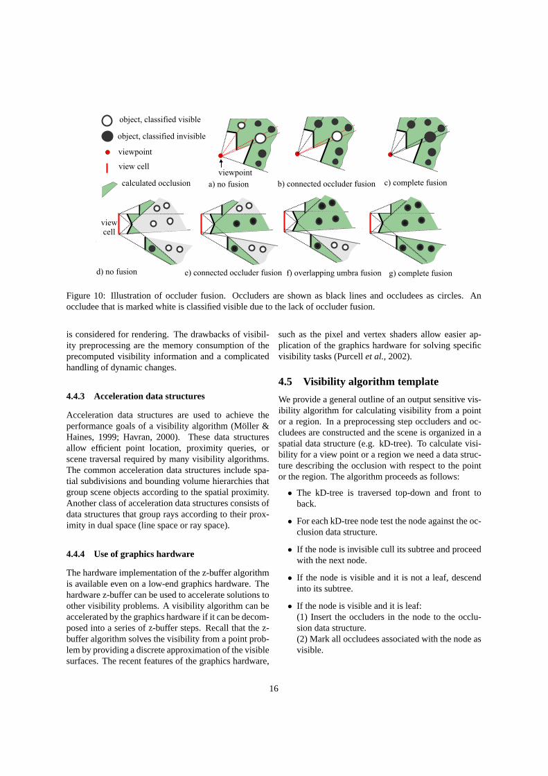
The occluder fusionis the ability of a visibility algo-rithm to account for the combined effect of multiple oc-cluders. We can distinguish three types of fusion of um-bra for visibility from a point algorithms. In the case ofvisibility from a region there are additional four typesthat express fusion of penumbra (see Figure 10).

4.4 Achieving performance

This section discusses four issues related to the runningtime and the memory consumption: scalability, acceler-ation data structures, and the use of graphics hardware.

4.4.1 Scalability

Scalability expresses the ability of the visibility algo-rithm to cope with larger inputs. The scalability of analgorithm can be studied with respect to the size of thescene (e.g. number of scene objects). Another measuremight consider the dependence of the algorithm on thenumber of the visible objects. Scalability can also bestudied according to the given domain restrictions, e.g.volume of the view cell.

A well designed visibility algorithm should be scal-able with respect to the number of structural changes ofvisibility. Furthermore, its performance should be givenby the complexity of the visible part of the scene. Thesetwo important measures of scalability of an algorithmare discussed in the next two sections.

Use of coherence Scenes in computer graphics typi-cally consist of objects whose properties vary smoothly.A view of such a scene contains regions of smoothchanges (changes in color, depth, texture,etc.) at thesurface of one object and discontinuities between ob-jects. The degree to which the scene or its projection ex-hibit local similarities is calledcoherence(Foleyet al.,1990). Coherence can be exploited by reusing calcula-tions made for one part of the scene for nearby parts.Algorithms exploiting coherence are typically more ef-ficient than algorithms computing the result from thescratch.

Sutherland et al. (1974) identified several differenttypes of coherence in the context of visible surface al-gorithms. We simplify the classification proposed bySutherland to reflect general visibility algorithms anddistinguish between the following three types ofvisibil-ity coherence:

• Spatial coherence. Visibility of points in spacetends to be coherent in the sense that the visiblepart of the scene consists of compact sets (regions)of visible and invisible points.

• Image-space, line-space, or ray-space coherence.Sets of similar rays tend to have the same visibil-ity classification, i.e. the rays intersect the sameobject.

• Temporal coherence. Visibility at two succes-sive moments is likely to be similar despite smallchanges in the scene or a region/point of interest.

The degree to which an algorithm exploits varioustypes of coherence is one of the major design paradigmsin research of new visibility algorithms. The impor-tance of exploiting coherence is emphasized by thelarge amount of data that need to be processed by thecurrent rendering algorithms.

Output sensitivity An algorithm is said to beoutputsensitiveif its running time is sensitive to the size ofoutput (Gotsmanet al., 1999). In the computer graph-ics community the term output sensitive algorithm isused in a broader meaning than in computational ge-ometry (Berget al., 1997). The attention is paid toa practical usage of the algorithm, i.e. to an efficientimplementation in terms of the practical average caseperformance. The algorithms are usually evaluated ex-perimentally using several data sets and measuring therunning time and the size of output of the algorithm.

4.4.2 Visibility preprocessing

Visibility computations at runtime can be accelerated byvisibility preprocessing. The time for preprocessing isoften amortized over many executions of runtime visi-bility queries (Moller & Haines, 1999). A typical appli-cation where visibility preprocessing is used are walk-throughs of complex geometric models (Aireyet al.,1990). In this case visibility is preprocessed by findinga PVS for all view cells in the scene. At run-time onlythe PVS corresponding to the location of the view point

15

viewpoint

a) no fusion c) complete fusion

e) connected occluder fusion

viewcell

d) no fusion f) overlapping umbra fusion g) complete fusion

b) connected occluder fusion

object, classified visible

object, classified invisible

viewpoint

view cell

calculated occlusion

Figure 10: Illustration of occluder fusion. Occluders are shown as black lines and occludees as circles. Anoccludee that is marked white is classified visible due to the lack of occluder fusion.

is considered for rendering. The drawbacks of visibil-ity preprocessing are the memory consumption of theprecomputed visibility information and a complicatedhandling of dynamic changes.

4.4.3 Acceleration data structures

Acceleration data structures are used to achieve theperformance goals of a visibility algorithm (Moller &Haines, 1999; Havran, 2000). These data structuresallow efficient point location, proximity queries, orscene traversal required by many visibility algorithms.The common acceleration data structures include spa-tial subdivisions and bounding volume hierarchies thatgroup scene objects according to the spatial proximity.Another class of acceleration data structures consists ofdata structures that group rays according to their prox-imity in dual space (line space or ray space).

4.4.4 Use of graphics hardware

The hardware implementation of the z-buffer algorithmis available even on a low-end graphics hardware. Thehardware z-buffer can be used to accelerate solutions toother visibility problems. A visibility algorithm can beaccelerated by the graphics hardware if it can be decom-posed into a series of z-buffer steps. Recall that the z-buffer algorithm solves the visibility from a point prob-lem by providing a discrete approximation of the visiblesurfaces. The recent features of the graphics hardware,

such as the pixel and vertex shaders allow easier ap-plication of the graphics hardware for solving specificvisibility tasks (Purcellet al., 2002).

4.5 Visibility algorithm template

We provide a general outline of an output sensitive vis-ibility algorithm for calculating visibility from a pointor a region. In a preprocessing step occluders and oc-cludees are constructed and the scene is organized in aspatial data structure (e.g. kD-tree). To calculate visi-bility for a view point or a region we need a data struc-ture describing the occlusion with respect to the pointor the region. The algorithm proceeds as follows:

• The kD-tree is traversed top-down and front toback.

• For each kD-tree node test the node against the oc-clusion data structure.

• If the node is invisible cull its subtree and proceedwith the next node.

• If the node is visible and it is not a leaf, descendinto its subtree.

• If the node is visible and it is leaf:(1) Insert the occluders in the node to the occlu-sion data structure.(2) Mark all occludees associated with the node asvisible.

16

Many efficient visibility culling algorithms follow thisoutline (Greeneet al., 1993; Bittneret al., 1998; Wonka& Schmalstieg, 1999; Downset al., 2001; Bittneret al.,2001; Wonkaet al., 2000). Graphics hardware can beused to accelerate the updates of the occlusion datastructure. On the other hand the occlusion test be-comes more complicated because of hardware restric-tions (Wonka & Schmalstieg, 1999; Durandet al., 2000;Zhanget al., 1997).

4.6 Summary

In this section we discussed common concepts of vis-ibility algorithm design and mentioned several criteriaused for the classification of visibility algorithms. Al-though the discussion was balanced towards visibilityculling methods we believe that it provides a usefuloverview even for other visibility problems.

To sum up the algorithms discussed in the paper weprovide two overview tables. Table 2 reviews algo-rithms for visibility from a point, Table 3 reviews al-gorithms for visibility from a line segment, a polygon,a region, and global visibility. The algorithms are in-dexed according to the problem domain, the actual vis-ibility problem, and the structure of the domain.

We characterize each algorithm using three features:solution space structure, solution space semantics, andaccuracy. These features were selected as they providea meaningful classification for the broad class of algo-rithms discussed in the paper. The solution space se-mantics is classified as follows: If the algorithm solvesvisibility in an image plane we classify it as imagespace. Note, that this plane does not need to corre-spond to the viewing plane (e.g. shadow map). Sim-ilarly, if the algorithm solves visibility using line spaceor ray space analogies, we classify it as line space orray space, respectively. If the algorithm solves visibilityusing object space entities (e.g. shadow volume bound-aries), we classify it as object space. The accuracy isexpressed with respect to the problem domain structure.This means that if the algorithm solves a problem witha discrete domain it can still provide an exact result al-though it evaluates visibility only for the discrete sam-ples.

5 Conclusion

Visibility problems and algorithms penetrate a largepart of computer graphics research. We proposed a tax-

onomy that aims to classify visibility problems inde-pendently of their target application. The classificationshould help to understand the nature of the given prob-lem and it should assist in finding relationships betweenvisibility problems and algorithms in different applica-tion areas.

We aimed to provide a representative sample of visi-bility algorithms for visible surface determination, vis-ibility culling, shadow computation, image-based andpoint-based rendering, global illumination, and globalvisibility computations.

We discussed common concepts of visibility algo-rithm design that should help to assist an algorithm de-signer to transfer existing algorithms for solving visi-bility problems. Finally, we summarized visibility algo-rithms discussed in the paper according to their domain,solution space, and accuracy.

Computer graphics offers a number of efficient visi-bility algorithms for all stated visibility problems in 2Das well as visibility along a line and visibility from apoint in 3D. In particular it provides a well researchedbackground for discrete techniques. The solution ofhigher dimensional visibility is significantly more dif-ficult. The discrete techniques require a large numberof samples to achieve satisfying accuracy, whereas thecontinuous techniques are prone to robustness problemsand are difficult to implement. The existing solutionsmust be tuned to a specific application. Therefore theproblems of visibility from a line segment, a polygon,a region, and global visibility problems in 3D are themain focus of active computer graphics research in vis-ibility.

Acknowledgments

This research was supported by the Czech Ministry ofEducation under Project LN00B096 and the AustrianScience Foundation (FWF) contract no. p-13876-INF.

17

problem solution spacedomain description domain algorithm structure semantics accuracy notes

structure

VFP

visiblesurface

determination

D

Catmull (1975) D I E HWNewellet al. (1972) C/D O/I EFuchset al. (1980) C/D O/I EGordon & Chen (1991) C/D O/I EWarnock (1969) D I EAppel (1968) D O E

CNaylor (1992) C O/I EWeiler & Atherton (1977) C I E

visibilityculling

D

Greeneet al. (1993) D I C HWZhanget al. (1997) D I C/A HWAila (2000) D I C/AHeyet al. (2001) D I C HWKlosowski & Silva. (2001) D I C HWCohen-Or & Shaked (1995) D O E terrainsLee & Shin (1997) D O E terrains

C

Luebke & Georges (1995) C I C indoorCoorg & Teller (1997) C O CHudsonet al. (1997) C O CBittneret al. (1998) C O CWonka & Schmalstieg (1999) D O C HWDownset al. (2001) C I C 21

2 DLloyd & Egbert (2002) C I C terrains

visibilitymaps

CStewart & Karkanis (1998) D I A HWBittner (2002a) C O/I E

hardshadows

D

Whitted (1979) D O EHaines & Greenberg (1986) D I CWoo & Amanatides (1990) D O CWilliams (1978) D I ASegalet al. (1992) D I A HWStamminger & Drettakis (2002) D I A HWCrow (1977) C/D O EHeidmann (1991) C/D O E HW

CChin & Feiner (1989) C O EChrysanthou & Slater (1995) C O E dynamic

ray-settracing

CHeckbert & Hanrahan (1984) C I EAmanatides (1984) C O ASzirmay-Kalos & Purgathofer (1998) D I A HW

point-basedrendering

D

McMillan (1997) D I EPfisteret al. (2000) D I ARusinkiewicz & Levoy (2000) D I A HWGrossman & Dally (1998) D I A HWWandet al. (2001) D I A HW

Problem domain structure: D - discrete, C - continuous.

Solution space structure: D - discrete, C - continuous.

Solution space semantics: O - object space, I - image space.

Accuracy: E - exact, C - conservative, A - approximate.

Table 2: Summary of visibility from a point algorithms.

18

problem solution spacedomain description domain algorithm structure semantics accuracy notes

structure

VLS

soft shadows D Heidrichet al. (2000) D I A HWvisibilitycullingin 21

2 DC

Wonkaet al. (2000) D O C HWKoltun et al. (2001) D O/L CBittneret al. (2001) C L/O C

VFPo

soft shadowsD Cooket al. (1984) D O A

C

Chin & Feiner (1992) C O AChrysanthou & Slater (1997) C O A dynamicHeckbert & Herf (1997) D I/O A HWSoler & Sillion (1998) D I/O A HW

form-factors CCohen & Greenberg (1985) D I A HWWallaceet al. (1989) D O ACampbell, III & Fussell (1990) C O A

discontinuitymeshing

C

Heckbert (1992) C O ALischinskiet al. (1992) C O ADrettakis & Fiume (1994) C O EStewart & Ghali (1994) C O E

VFRvisibilityculling

C

Durandet al. (2000) D I/O C HWSchaufleret al. (2000) D O CBittner (2002b) C L ENirensteinet al. (2002) C L EAirey et al. (1990) D O A indoorTeller & Sequin (1991) C L E indoor 2DTeller (1992b) C L E indoorYagel & Ray (1995) D O C cavesStewart (1997) C O C terrain

GV

aspect graph C Plantingaet al. (1990) C O E

visibilitycomplex

C

Pocchiola & Vegter (1993) C L E 2DRiviere (1997) C L E 2DDurandet al. (1996) C L EDurandet al. (1997) C O EDuguet & Drettakis (2002) C O E/A

discretestructures

C

Hinkenjann & Muller (1996) D L A 2DBlais & Poulin (1998) D L AChrysanthouet al. (1998) D R AGotsmanet al. (1999) D R A

Problem domain structure: D - discrete, C - continuous.Solution space structure: D - discrete, C - continuous.Solution space semantics: O - object space, L - line space, R - ray space.Accuracy: E - exact, C - conservative, A - approximate.

Table 3: Summary of algorithms for visibility from a line segment, visibility from a polygon, visibility from aregion, and global visibility.

19

ReferencesAila, T. (2000).SurRender Umbra: A Visibility Determina-

tion Framework for Dynamic Environments. Master’s the-sis, Helsinki University of Technology.

Airey, J.M., Rohlf, J.H. & Brooks, Jr., F.P. (1990). Towardsimage realism with interactive update rates in complex vir-tual building environments. In1990 Symposium on Inter-active 3D Graphics, 41–50, ACM SIGGRAPH.

Amanatides, J. (1984). Ray tracing with cones. InComputerGraphics (SIGGRAPH ’84 Proceedings), vol. 18, 129–135.

Appel, A. (1968). Some techniques for shading machine ren-derings of solids. InAFIPS 1968 Spring Joint ComputerConf., vol. 32, 37–45.

Arvo, J. & Kirk, D. (1989).A survey of ray tracing accelera-tion techniques, 201–262. Academic Press.

Arvo, J. & Kirk, D. (1990). Particle transport and image syn-thesis. In F. Baskett, ed.,Computer Graphics (Proceedingsof SIGGRAPH’90), 63–66.

Berg, M., Kreveld, M., Overmars, M. & Schwarzkopf, O.(1997).Computational Geometry: Algorithms and Appli-cations. Springer-Verlag, Berlin, Heidelberg, New York.

Bittner, J. (2002a). Efficient construction of visibility mapsusing approximate occlusion sweep. InProceedings ofSpring Conference on Computer Graphics (SCCG’02),163–171, Budmerice, Slovakia.

Bittner, J. (2002b).Hierarchical Techniques for VisibilityComputations. Ph.D. thesis, Czech Technical University inPrague.

Bittner, J., Havran, V. & Slavık, P. (1998). Hierarchicalvisibility culling with occlusion trees. InProceedings ofComputer Graphics International ’98 (CGI’98), 207–219,IEEE.

Bittner, J., Wonka, P. & Wimmer, M. (2001). Visibility pre-processing for urban scenes using line space subdivision. InProceedings of Pacific Graphics (PG’01), 276–284, IEEEComputer Society, Tokyo, Japan.

Blais, M. & Poulin, P. (1998). Sampling visibility in three-space. InProc. of the 1998 Western Computer GraphicsSymposium, 45–52.

Campbell, III, A.T. & Fussell, D.S. (1990). Adaptive meshgeneration for global diffuse illumination. InComputerGraphics (SIGGRAPH ’90 Proceedings), vol. 24, 155–164.

Carpenter, L. (1984). The A-buffer, an antialiased hidden sur-face method. In H. Christiansen, ed.,Computer Graphics(SIGGRAPH ’84 Proceedings), vol. 18, 103–108.

Catmull, E.E. (1975). Computer display of curved surfaces. InProceedings of the IEEE Conference on Computer Graph-ics, Pattern Recognition, and Data Structure, 11–17.

Chin, N. & Feiner, S. (1989). Near real-time shadow genera-tion using BSP trees. InComputer Graphics (Proceedingsof SIGGRAPH ’89), 99–106.

Chin, N. & Feiner, S. (1992). Fast object-precision shadowgeneration for areal light sources using BSP trees. InD. Zeltzer, ed.,Computer Graphics (1992 Symposium onInteractive 3D Graphics), vol. 25, 21–30.

Chrysanthou, Y. & Slater, M. (1995). Shadow volume BSPtrees for computation of shadows in dynamic scenes. InP. Hanrahan & J. Winget, eds.,1995 Symposium on In-teractive 3D Graphics, 45–50, ACM SIGGRAPH, iSBN0-89791-736-7.

Chrysanthou, Y. & Slater, M. (1997). Incremental updates toscenes illuminated by area light sources. InProceedings ofEurographics Workshop on Rendering, 103–114, SpringerVerlag.

Chrysanthou, Y., Cohen-Or, D. & Lischinski, D. (1998). Fastapproximate quantitative visibility for complex scenes.In Proceedings of Computer Graphics International ’98(CGI’98), 23–31, IEEE, NY, Hannover, Germany.

Cohen, M.F. & Greenberg, D.P. (1985). The hemi-cube: Aradiosity solution for complex environments.ComputerGraphics (SIGGRAPH ’85 Proceedings), 19, 31–40.

Cohen-Or, D. & Shaked, A. (1995). Visibility and dead-zonesin digital terrain maps.Computer Graphics Forum, 14,C/171–C/180.

Cohen-Or, D., Chrysanthou, Y., Silva, C. & Durand, F. (2002).A survey of visibility for walkthrough applications.To ap-pear in IEEE Transactions on Visualization and ComputerGraphics..

Cook, R.L., Porter, T. & Carpenter, L. (1984). Distributed raytracing. InComputer Graphics (SIGGRAPH ’84 Proceed-ings), 137–45.

Coorg, S. & Teller, S. (1997). Real-time occlusion culling formodels with large occluders. InProceedings of the Sympo-sium on Interactive 3D Graphics, 83–90, ACM Press, NewYork.

Crow, F.C. (1977). Shadow algorithms for computer graphics.Computer Graphics (SIGGRAPH ’77 Proceedings), 11.

Downs, L., Moller, T. & Sequin, C.H. (2001). Occlusion hori-zons for driving through urban scenes. InSymposium onInteractive 3D Graphics, 121–124, ACM SIGGRAPH.

20

Drettakis, G. & Fiume, E. (1994). A Fast Shadow Algorithmfor Area Light Sources Using Backprojection. InComputerGraphics (Proceedings of SIGGRAPH ’94), 223–230.

Duguet, F. & Drettakis, G. (2002). Robust epsilon visibility.Computer Graphics (SIGGRAPH’02 Proceedings).

Durand, F. (1999).3D Visibility: Analytical Study and Appli-cations. Ph.D. thesis, Universite Joseph Fourier, Grenoble,France.

Durand, F., Drettakis, G. & Puech, C. (1996). The 3D visi-bility complex: A new approach to the problems of accu-rate visibility. In Proceedings of Eurographics RenderingWorkshop ’96, 245–256, Springer.

Durand, F., Drettakis, G. & Puech, C. (1997). The visibil-ity skeleton: A powerful and efficient multi-purpose globalvisibility tool. In Computer Graphics (Proceedings of SIG-GRAPH ’97), 89–100.

Durand, F., Drettakis, G., Thollot, J. & Puech, C. (2000). Con-servative visibility preprocessing using extended projec-tions. InComputer Graphics (Proceedings of SIGGRAPH2000), 239–248.

Floriani, L.D. & Magillo, P. (1995). Horizon computation ona hierarchical terrain model.The Visual Computer: An In-ternational Journal of Computer Graphics, 11, 134–149.

Foley, J.D., van Dam, A., Feiner, S.K. & Hughes, J.F. (1990).Computer Graphics: Principles and Practice. Addison-Wesley Publishing Co., Reading, MA, 2nd edn.

Fuchs, H., Kedem, Z.M. & Naylor, B.F. (1980). On visiblesurface generation by a priori tree structures. InComputerGraphics (SIGGRAPH ’80 Proceedings), vol. 14, 124–133.

Funkhouser, T., Carlbom, I., Elko, G., Pingali, G., Sondhi,M. & West, J. (1998). A beam tracing approach to acousticmodeling for interactive virtual environments. InComputerGraphics (Proceedings of SIGGRAPH ’98), 21–32.

Goral, C.M., Torrance, K.K., Greenberg, D.P. & Battaile, B.(1984). Modelling the interaction of light between diffusesurfaces. InComputer Graphics (SIGGRAPH ’84 Proceed-ings), vol. 18, 213–222.

Gordon, D. & Chen, S. (1991). Front-to-back display of BSPtrees.IEEE Computer Graphics and Applications, 11, 79–85.

Gortler, S.J., Grzeszczuk, R., Szeliski, R. & Cohen, M.F.(1996). The lumigraph. InComputer Graphics (SIG-GRAPH ’96 Proceedings), Annual Conference Series, 43–54, Addison Wesley.

Gotsman, C., Sudarsky, O. & Fayman, J.A. (1999). Opti-mized occlusion culling using five-dimensional subdivi-sion.Computers and Graphics, 23, 645–654.

Grant, C.W. (1992).Visibility Algorithms in Image Synthesis.Ph.D. thesis, U. of California, Davis.

Grasset, J., Terraz, O., Hasenfratz, J.M. & Plemenos, D.(1999). Accurate scene display by using visibility maps.In Spring Conference on Computer Graphics and its Ap-plications.

Greene, N., Kass, M. & Miller, G. (1993). Hierarchical Z-buffer visibility. In Computer Graphics (Proceedings ofSIGGRAPH ’93), 231–238.

Grossman, J.P. & Dally, W.J. (1998). Point sample rendering.In Rendering Techniques ’98 (Proceedings of Eurograph-ics Rendering Workshop), 181–192, Springer-Verlag WienNew York.

Gu, X., Gortier, S.J. & Cohen, M.F. (1997). Polyhedral ge-ometry and the two-plane parameterization. In J. Dorsey& P. Slusallek, eds.,Eurographics Rendering Workshop1997, 1–12, Eurographics, Springer Wein, New York City,NY, iSBN 3-211-83001-4.

Haines, E.A. & Greenberg, D.P. (1986). The light buffer:A ray tracer shadow testing accelerator.IEEE ComputerGraphics and Applications, 6, 6–16.

Havran, V. (2000).Heuristic Ray Shooting Algorithms. Ph.d.thesis, Department of Computer Science and Engineering,Faculty of Electrical Engineering, Czech Technical Univer-sity in Prague.

Heckbert, P.S. (1992). Discontinuity meshing for radiosity.In Third Eurographics Workshop on Rendering, 203–216,Bristol, UK.

Heckbert, P.S. & Hanrahan, P. (1984). Beam tracing polygo-nal objects.Computer Graphics (SIGGRAPH’84 Proceed-ings), 18, 119–127.

Heckbert, P.S. & Herf, M. (1997). Simulating soft shadowswith graphics hardware. Tech. rep., CS Dept., CarnegieMellon U., cMU-CS-97-104, http://www.cs.cmu.edu/ ph.

Heidmann, T. (1991). Real shadows, real time.Iris Universe,18, 28–31, silicon Graphics, Inc.

Heidrich, W., Brabec, S. & Seidel, H. (2000). Soft shadowmaps for linear lights. InProceedings of EUROGRAPHICSWorkshop on Rendering, 269–280.

Hey, H., Tobler, R.F. & Purgathofer, W. (2001). Real-Time oc-clusion culling with a lazy occlusion grid. InProceedingsof EUROGRAPHICS Workshop on Rendering, 217–222.

21

Hinkenjann, A. & Muller, H. (1996). Hierarchical blockertrees for global visibility calculation. Research Report621/1996, University of Dortmund.

Hudson, T., Manocha, D., J.Cohen, M.Lin, K.Hoff &H.Zhang (1997). Accelerated occlusion culling usingshadow frusta. InProceedings of the Thirteenth ACM Sym-posium on Computational Geometry, June 1997, Nice,France.

Kajiya, J.T. (1986). The rendering equation. InComputerGraphics (SIGGRAPH ’86 Proceedings), 143–150.

Klosowski, J.T. & Silva., C.T. (2001). Efficient conservativevisibility culling using the prioritized-layered projectionalgorithm. IEEE Transactions on Visualization and Com-puter Graphics, 7, 365–379.

Koltun, V., Chrysanthou, Y. & Cohen-Or, D. (2001).Hardware-accelerated from-region visibility using a dualray space. InProceedings of the 12th EUROGRAPHICSWorkshop on Rendering.

Lee, C.H. & Shin, Y.G. (1997). A terrain rendering methodusing vertical ray coherence.The Journal of Visualizationand Computer Animation, 8, 97–114.

Levoy, M. & Hanrahan, P. (1996). Light field rendering.In H. Rushmeier, ed.,SIGGRAPH 96 Conference Pro-ceedings, Annual Conference Series, 31–42, ACM SIG-GRAPH, Addison Wesley, held in New Orleans, Louisiana,04-09 August 1996.

Lischinski, D., Tampieri, F. & Greenberg, D.P. (1992). Dis-continuity meshing for accurate radiosity.IEEE ComputerGraphics and Applications, 12, 25–39.

Lloyd, B. & Egbert, P. (2002). Horizon occlusion culling forreal-time rendering of hierarchical terrains. InProceed-ings of the conference on Visualization ’02, 403–410, IEEEPress.

Luebke, D. & Georges, C. (1995). Portals and mirrors: Sim-ple, fast evaluation of potentially visible sets. In P. Hanra-han & J. Winget, eds.,1995 Symposium on Interactive 3DGraphics, 105–106, ACM SIGGRAPH.

McMillan, L. (1997). An image-based approach to three-dimensional computer graphics. Ph.D. Thesis TR97-013,University of North Carolina, Chapel Hill.

Moller, T. & Haines, E. (1999).Real-Time Rendering. A. K.Peters Limited.

Naylor, B.F. (1992). Partitioning tree image representationand generation from 3D geometric models. InProceedingsof Graphics Interface ’92, 201–212.

Newell, M.E., Newell, R.G. & Sancha, T.L. (1972). A solu-tion to the hidden surface problem. InProceedings of ACMNational Conference.

Nirenstein, S., Blake, E. & Gain, J. (2002). Exact From-Region visibility culling. InProceedings of EUROGRAPH-ICS Workshop on Rendering, 199–210.

Pellegrini, M. (1997). Ray shooting and lines in space. In J.E.Goodman & J. O’Rourke, eds.,Handbook of Discrete andComputational Geometry, chap. 32, 599–614, CRC PressLLC, Boca Raton, FL.

Pfister, H., Zwicker, M., van Baar, J. & Gross, M. (2000).Surfels: Surface elements as rendering primitives. InCom-puter Graphics (Proceedings of SIGGRAPH 2001), 335–342, ACM SIGGRAPH / Addison Wesley Longman.

Plantinga, H., Dyer, C.R. & Seales, W.B. (1990). Real-timehidden-line elimination for a rotating polyhedral scene us-ing the aspect representation. InProceedings of GraphicsInterface ’90, 9–16.

Pocchiola, M. & Vegter, G. (1993). The visibility complex. InProc. 9th Annu. ACM Sympos. Comput. Geom., 328–337.

Purcell, T.J., Buck, I., Mark, W.R. & Hanrahan, P. (2002). Raytracing on programmable graphics hardware. InComputerGraphics (SIGGRAPH ’02 Proceedings), 703–712.

Riviere, S. (1997). Dynamic visibility in polygonal sceneswith the visibility complex. InProc. 13th Annu. ACM Sym-pos. Comput. Geom., 421–423.

Rusinkiewicz, S. & Levoy, M. (2000). QSplat: A multires-olution point rendering system for large meshes. InCom-puter Graphics (Proceedings of SIGGRAPH 2000), 343–352, ACM SIGGRAPH / Addison Wesley Longman.

Saona-Vazquez, C., Navazo, I. & Brunet, P. (1999). The visi-bility octree: a data structure for3D navigation.Computersand Graphics, 23, 635–643.

Schaufler, G., Dorsey, J., Decoret, X. & Sillion, F.X. (2000).Conservative volumetric visibility with occluder fusion. InComputer Graphics (Proceedings of SIGGRAPH 2000),229–238.

Segal, M., Korobkin, C., van Widenfelt, R., Foran, J. & Hae-berli, P. (1992). Fast shadows and lighting effects using tex-ture mapping.Computer Graphics (SIGGRAPH ’92 Pro-ceedings), 26, 249–252.

Soler, C. & Sillion, F. (1998). Fast calculation of soft shadowtextures using convolution. InComputer Graphics (Pro-ceedings of SIGGRAPH ’98), ACM SIGGRAPH.

22

Stamminger, M. & Drettakis, G. (2002). Perspective shadowmaps. InSIGGRAPH 2002 Conference Proceedings, 557–562, ACM Press/ ACM SIGGRAPH.

Stewart, A.J. (1997). Hierarchical visibility in terrains. InPro-ceedings of Eurographics Rendering Workshop ’97, 217–228.

Stewart, A.J. & Ghali, S. (1994). Fast computation of shadowboundaries using spatial coherence and backprojections.In Computer Graphics (Proceedings of SIGGRAPH ’94),231–238.

Stewart, A.J. & Karkanis, T. (1998). Computing the approx-imate visibility map, with applications to form factors anddiscontinuity meshing. InProceedings of the Ninth Euro-graphics Workshop on Rendering, 57–68.

Stolfi, J. (1991).Oriented Projective Geometry: A Frameworkfor Geometric Computations. Academic Press.

Sutherland, I.E., Sproull, R.F. & Schumacker, R.A. (1974).A characterization of ten hidden-surface algorithms.ACMComputing Surveys, 6, 1–55.

Szirmay-Kalos, L. & Purgathofer, W. (1998). Global ray-bundle tracing with hardware acceleration. InNinth Euro-graphics Workshop on Rendering, Vienna, Austria.

Teller, S.J. (1992a). Computing the antipenumbra of an arealight source. InComputer Graphics (Proceedings of SIG-GRAPH ’92), 139–148.

Teller, S.J. (1992b).Visibility Computations in Densely Oc-cluded Polyhedral Environments. Ph.D. thesis, CS Divi-sion, UC Berkeley, tech. Report UCB/CSD-92-708.

Teller, S.J. & Sequin, C.H. (1991). Visibility preprocess-ing for interactive walkthroughs. InProceedings of SIG-GRAPH ’91, 61–69.

Wald, I., Slusallek, P., Benthin, C. & Wagner, M.(2001). Interactive rendering with coherent ray tracing. InA. Chalmers & T.M. Rhyne, eds.,EG 2001 Proceedings,vol. 20(3) ofComputer Graphics Forum, 153–164, Black-well Publishing.

Wallace, J.R., Elmquist, K.A. & Haines, E.A. (1989). A raytracing algorithm for progressive radiosity. InSIGGRAPH’89 Proceedings, 315–324.

Wand, M., Fischer, M., Peter, I., auf der Heide, F.M. &Straßer, W. (2001). The randomized z-buffer algorithm:Interactive rendering of highly complex scenes. InCom-puter Graphics (Proceedings of SIGGRAPH 2001), 361–370, ACM SIGGRAPH.

Warnock, J. (1969). A hidden-surface algorithm for computergenerated half-tone pictures. Tech. Rep. TR 4–15, NTISAD-733 671, University of Utah, Computer Science De-partment.

Weiler, K. & Atherton, P. (1977). Hidden surface removalusing polygon area sorting. InComputer Graphics (SIG-GRAPH ’77 Proceedings), 214–222.

Whitted, T. (1979). An improved illumination model forshaded display. InComputer Graphics (Special SIG-GRAPH ’79 Issue), vol. 13, 1–14.

Williams, L. (1978). Casting curved shadows on curved sur-faces. InComputer Graphics (SIGGRAPH ’78 Proceed-ings), 270–274.

Wonka, P. & Schmalstieg, D. (1999). Occluder shadows forfast walkthroughs of urban environments. InComputerGraphics Forum (Proceedings of EUROGRAPHICS ’99),51–60, Blackwell Publishers.

Wonka, P., Wimmer, M. & Schmalstieg, D. (2000). Visi-bility preprocessing with occluder fusion for urban walk-throughs. InProceedings of EUROGRAPHICS Workshopon Rendering, 71–82.

Woo, A. & Amanatides, J. (1990). Voxel occlusion testing: Ashadow determination accelerator for ray tracing. InPro-ceedings of Graphics Interface ’90, 213–220.

Woo, A., Poulin, P. & Fournier, A. (1990). A survey ofshadow algorithms.IEEE Computer Graphics and Appli-cations, 10, 13–32.

Yagel, R. & Ray, W. (1995). Visibility computation for ef-ficient walkthrough of complex environments.Presence:Teleoperators and Virtual Environments, 5.

Zhang, H., Manocha, D., Hudson, T. & Hoff III, K.E. (1997).Visibility culling using hierarchical occlusion maps. InComputer Graphics (Proceedings of SIGGRAPH ’97), 77–88.

23