visible emissions field manual, epa methods 9 and 22 · pdf filevisible emissions field manual...

EPA 340/l -92-004 December 1993

Visible Emissions Field Manual EPA Methods 9 and 22

Prepared by:

Eastern Technical Associates PO Box 58495

Raleigh, NC 27658

and

Entrophy Environmentalist, Inc. PO Box 12291

Research Triangle Park, NC 27709 .

! / ’ -r-F> ;... VP.’ Contract No. 68-02-4462

6 .$,’ * Work Assignment No. 91-188

EPA Work Assignment Managers: Karen Randolph and Kirk Foster El?+ Project Officer: Aaron Martin

/

I

US. ENVIRONMENTAL PROTECTION AGENCY Stationary Source Compliance Division

Office of Air Quality Planning and Standards Washington, DC 20460

December 1993

Contents

Introduction .................... ..“....“..........“..“““....“..“........”....”....“....“........................“....““....” ... 2

A Brief History of Opacity . ..“............“..“......H..................”................................“......“......”..”” . 3

Opacity Measurement Principles .. ..“..........“..“..........................”..............................“....” ......... 4

Records Review . . . . . . . . . . . . . . . . . . . . . . . . . . . . . . . . . . . . . . . . . . . . . . . . . . . . . . . . . . . . . . . . . . . . . . . . . . . . . . . . . ..“............“....................”..... 8

Equipment . . . . . . . . . . . . . . . . . . . ..“................................”............................................................................. 9

Field Operations . . . . . . . . . . . . . . . . . . . . . . . . . . . . . . . . . . . . . . . . . . . . . . . . . . . . . . . . . ..“............................................................. 11

Calculations . . . . . . . . . . . . . . . . . . . . . . . . . . . . . . . . . . . . . . . . . . . . . . . . . . . . . . . . . . . . . . . . . . . . . . . . . . . . . . . . . . . . . . . . . . . . . . . . . . . . . . . . . . . . . . . . . . . . . . . . ..*....... 14

Data Review . . . . . . . . . . . . . . . . . . . . . . . . . . . . . . . . . . . . . . . . . . . . . . ..“......““..................................................................... 15

Appendix A: Forms

Appendix B: Method 9

Appendix C: Method 22

Jntroduction

The Federal opacity standards for various industries are found in 4OCPR Part 60 (Standards of Performance for New and Modified Stationary Sources) and 40 CFR Part 61 and 62 (Emission Standards for Hazardous Air Pol- lutants). These standards require the use of Reference Method 9 or Reference Method 22, contained in Appen- dix A of Part 60, for the determination of the level or frequency of visible emissions by trained observers.

In addition to the plume observation procedures, Method 9 also contains data reduction and reporting procedures as well as procedures and specifications for training and certifying qualified visible emission (VIZ) observers.

State Implementation Plans (SIPS) also typically include several types of opacity regulations, which in some cases may differ from the federal opacity standards in terms of the opacity limits, the measurement method or test procedure, or the data evaluation technique. For example, some SIP opacity rules limit visible emissions to a specified number of minutes per hour or other time period (time exemption); some limit opacity to a certain level averaged over a specified number of minutes (time averaged): some set opacity limits where no single reading can exceed the standard (instantanous or “‘cap”). Re- gardless of the exact format of the SIP opacity regulations. nearly all use the procedures in Method 9 for conducting VE field observations and for training and cenifying VE observers. The observation procedums contain instructions on how to read the plume and record the values, including where to stand to observe the plume and what information must be gathered to support the visible emission determinations. Thi validity of the VII determinations used for compliance or noncompliance demonstration purposes depends to a great extent on how well the field observations are documented on the VE Observation Form. This field manual will stress the type and extent of documentation needed to satisfy Method 9 requirements.

Federal opacity standards and most SIP opacity regulations are independently enforceable, i.e., a source may be cited for an opacity violation even when it is in compliance with the particulate mass standard Thus, visible emission observations by qualified agency observers serve

as a primary compliance surveillance tool for enforcement of emission control standards. In addition, many federal and SIP regulations and construction and operating permits also require owners/operators of affected fa- cilities to assess and report opacity data during the initial compliance tests and at specified intervals over the long term.

Regulated sources may be subject to stiff penalties for failure to comply with federal and state emission standards, including opacity standards. Civil and adminis- trative penalties of up to $25,000 per day per violation can be assessed under the Clean Air Act (CM). States and local agencies are encouraged under Title V of the CM to have program authority to levy fines up to $10,000 per day per violation. Therefore, visible emission determinations for compliance demonstration or enforcement purposes must be made accurately and must be suffi- ciently well documented to withstand rigorous examina- tion in potential enforcement proceedings, admiitrative or legal hearings, or eventual court litigation.

Produd errors or omissions on the visible emission evaluation forms or data sheets can invalidate the data or otherwise provide a basis for questioning the evaluation. only by carefully following the procedures set forth in Method 9 (or any other reference method) and by paying close attention to proper completion of the m Observa- tion Form can you be assured of acceptance of the evaluation data.

The purpose of this simplified manual is to present a stepby-step field guide for inexperienced VE observers who have recently completed the VIZ training and certification tests on how to conduct VE observations in accordance with the published opacity methods. The basic steps of a well-planned and properly performed VE inspection are i.Uust.tated in the inspection flow chart (see Figure 1). This manual is organized to follow the inspection flow chart Sections of the reference methods that must be carefully observed or followed during the inspection are highlighted. Method 9 and Method 22 are reprinted in full in Appendix B and Appendix C respec- tively. A recommended field VE Observation Form, in- eluded in Appendix A, may be copied or modified for field use.

.

It should be noted that much of the information presented in this simplified field manual has been derived f&m a number of previously published technical guides, manuals. and reports on Method 9 and related opacity

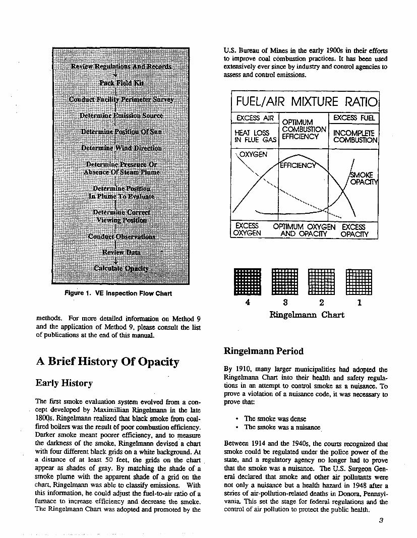
Figure 1. VE inspection Flow Chart

methods. For more detailed information on Method 9 and the application of Method 9, please consult the list of publications at the end of this manual.

A Brief History Of Opacity

Early History

The first smoke evaluation system evolved from a con- cept developed by MaximilIian Ringelmann in the late 18Oqs. Ringehnann realized that black smoke from coal- fired boilers was the result of poor combustion efficiency. Darker smoke meant poorer efficiency, and to measure the darkness of the smoke, Ringelmann devised a chart with four different black grids on a white background. At a. distance of at least 50 feet, the grids on the chart

appear as shades of gray. By matching the shade of a smoke plume with the apparent shade of a grid on the chart, Ringelmann was able to classify emissions. With this information, he could adjust the fuel-to-air ratio of a furnace to increase efficiency and decrease the smoke. The Ringelmann Chart was adopted and promoted by the

U.S. Bureau of Mines in the early 1900s in their efforts to improve coal combustion practices. It has beeu used extensively ever since by industry and control agencies to assess and control emissions.

FUEL/AIR MIXTURE RATIO

. EXCESS AIR OPTIMUM EXCESS FUEL

HEAT LOSS IN FLUE GAS

&g&m$N INCOMPLETE COMBUSTION

D(CESS OXYGEN

OP71hl;Mw~~$EN EXCESS OPACITY

4 3 2 1

Ringelmam Chart

Ringelmann Period

By 1910. many larger municipalities had adopted the Ringelmann Chart into their health and safety reguIa- tions in an attempt to control smoke as a nuisance. To prove a violation of a nuisance code, it was necessary to prove that:

l The smoke was dense l The smoke was a nuisauce

Between 1914 and the 1940s. the courts recognized that smoke could be regulated under the police power of the state, and a regulatory agency no longer had to prove that the smoke was a nuisance. The U.S. Surgeon Gen- eral declared that smoke and other air pollutants were not only a nuisance but a health hazard in 1948 after a series of air-pollution-related deaths in Donora, Pennsyl- vania This set the stage for federal regulations and the control of air pollution to protect the public health.

3

.

Equivalent Opacity

In the 1950s and 1960s Los Angeles added two major refinements to the use of visible emissions as a tool for controlling particulate emissions. The Ringelmann method

’ was expanded to white and other colors of smoke by the introduction of “equivalent opacity.” Equivalent opacity meant that the white smoke was equivalent to a Ringelmann number in its ability to obscure the view of a background. In some states, equivalent opacity is still measured in Ringelmann numbers, whereas in others the O-to 100~percent scale is used. Also, by training and certifying inspectors using a smoke generator equipped with an opacity meter, regulatory agencies ensured that certified inspectors did not have to carry and use Ringelmann cards.

In 1968, the Federal Air Pollution Control Office published AP-30. Optical properties and Visual Effects of Smoke-Stack Plumes, describing the accuracy of a smoke reader’s observations compared to a tmnsmissometer. AP- 30 also discussed the effect on opacity observations when a plume is viewed with the sun in the wrong place relative to the source.

Method 9

The Environmental Protection Agency (EPA) stopped using Ringelmann numbers in the New Source performance Standards when the revised EPA Method 9 was promulgated in 1974. All NSPS visible emission limits are stated in percent opacity units. Although some state regulations (notably California’s) still specify the use of the Ringelmann system for black and gray plumes, the national trend is to read all emissions in percent opacity.

EPA conducted extensive field studies on the accmacy and reliability of the Method 9 opacity evaluation technique when the method was revised and repromulgated in response to industry challenges concerning certain NSPS opacity standards and methods. The studies showed that visible emissions can be assessed accurately by prop erly trained and certXed observers. Two central features of Method 9 involve taking opacity readings of plumes at Wsecond intervals and averaging 24 consecutive readings (6 minutes) unless some other time period is specified in the emission standard (some NSPS specify a 3-minute averaging period).

Plume opacity emission standards and requirements remain the mainstay of federal, state, and local enforcement efforts. Today, more visible emission observers are certified annually than at any time in the past. This certification rate will continue to increase with the increase of federal and state regulations on industrial processes and combustion sources such as municipal, medical,

and hazardous waste incinerators. Visible emissions standa& are also applied extensively in controlling fugitive emissions ‘km both industrial processes and non-process dust sources such as roads and bulk materials stor- age and handling areas. Often there are no convenient accurate stack te’sting methods for measurement of emissions from unconfined sources other than opacity methods.

Method 22

Since EPA promulgated Method 22 in 1982, it has become an important tool in the conaol of visible emissions. Method 22 is a qualitative technique that checks only the presence or absence of visible emissions. Method 22 or a similar method is often used in the regulation of fugitive emissions of toxic mater&. Unlike with Method 9, Method 22 users don’t have to be certified. However, a knowledge of observation techniques is essential for correct use of the method. Therefore, Method 22 requires the observer to e trained by attending the lecture and field practice session of the Method 9 smoke school.

Opacity Measurement Principles

The relationships between light transmittance, plume opacity, and Ringelmann numbers are presented in Table 1.

Table 1. Comparison of Ringelmann Number, Plume Opacity, and Light Transmittance

A literal definition of plume opacity is the degree to which the transmission of light is reduced or the degree to which the visibility of a background as viewed through

the diameter of a plume is reduced. In simpler terms, opacity is the obscuring power of the plume, expressed in

percent. In physical terms, opacity is dependent upon transmittance (I/I) through the plume, where IO is the incident light flux and I is the light flux leaving the plume along the same light path. Percent opacity can be calculated using the following equation:

Percent opacity = (l-U(I) x 100.

Variables Influencing Opacity Observations

Method 9 advises:

The appearance of a plume as viewed by an observer depends upon a number of variables, some of which might be controllable and some of which might not be controllable in the field

The factors that influence plume opacity readings include particle density, particle refractive index, particle size distribution, particle color, plume background, pathlength, distance and relative eleva- tion to stack exit, sun angle, and lighting conditions.

Particle size is particularly significant; particles decrease light transmission by both scattering and direct absorp- tion. Particles with diameters approximately equal to the wavelength of visible light (0.4 to 0.7 pm) have the greatest scattering effect and cause the highest opacity. For a given mass emission rate, smaller particles will cause a higher opacity effect than larger particles. You should note that particles in the size range of 05 pm to 8 pm which typically cause most of the plume opacity, are also in the respimble range and are designated as PM,, particles.

Variables that might be controllable in the field arc luminous contrast and color contrast between the plume and the background against which the plume is viewed. These variables exert an influence on the appearance of a plume and can affect an observer’s ability to assign opacity values accurately. For example, when either contrast is high, the effect of the plume on the background is more evident and opacity values can be assigned with greater accuracy. When both contrasts are low, such as in the case of a gray plume on an overcast cloudy day. the effect is low and negative errors will occur. A negative error is when the observer under-estimates the true opacity of the plume.

An example of high luminous contrast is a black plume against a light sky. Two objects of the same color could show up against each other because of differences in lighting levels or light direction. This effect is particularly important when the sun is behind a plume, thereby making the plume more luminous than the background

and creating a high .bii (positive error) in opacity readings. On the other hand, when the sun is properly oriented in relation to the plume and the plume color is identical with the background color, observers will gen- erally have diffculty distinguishing between the plume and the background.

The line-of-sight pathlength through the plume is of par- ticular concern. Method 9 states:

. ..the observer shall, as much as possible, make his observations from a position such that his line of vision is approximately perpendicular to the plume direction, and when observing opacity of emissions from rectangular outlets (e.g., roof monitors, open baghouses, noncircular stacks), approximately perpendicular to the longer axis of the outlet.

If the line of sight varies more than 18’ fiorn the perpendicular, a positive error greater than 1 percent occurs. As the angle increases, the error increases. When observing plumes from conventional sources, observers should stand at least three stack distances away from a vertically ris- ing plume to meet this requirement. When observing plumes from fugitive so&es, which are rarely perfectly round and are strongly affected by the wind, observers must take care to meet this requirement.

5

Measurement Error

All measurement systems have an associated error, and Method 9 is no exception. As a result of field trials conducted at the time Method 9 was promulgated, the error levels at two confidence intervals for white and black smoke using Method 9 were determined. The method states:

. .Foc black plumes (133 sets at a smoke generator) lOO.percent of the sets [average of 25 readings] were read with a positive error of less than 7.5 percent opacity; 99 percent were read with a positive error of less than 5 percent opacity.

For white plumes (170 sets at a smoke generator, 168 sets at a coal-f& power plant, 298 sets at a sulfuric acid plant), 99 percent of the sets were read with a positive error of less than 7.5 percent opacity; 95 percent were read with a positive error of less than 5 percent opacity.

. This means that during these field trials 100 percent of the b&k,plumes and 99 percent of the white plumes were nQ@verread by more than 75*percent opacity. In other Gords, there is only a l-percent chance that an observer will exceed the error on a white plume and no chance that an observer will exceed the error on a black plume. Negative biases due to low-contrast observation conditions will often further offset the &@vational error.

Ninety-nine percent of the black plumes and 95 percent of the white plumes were read within 5 percent opacity. This means that an oveneading occurs only about once in 20 readings. Again, negative biases that result from poor observation conditions (low plume-to-tjackground contrast) reduce the positive observational error.

studies also showed that positive error is reduced by in- creasing Ihe number of observations in either averaging time or in number of averages. Both techniques improve the accuracy of the method.

Method 22

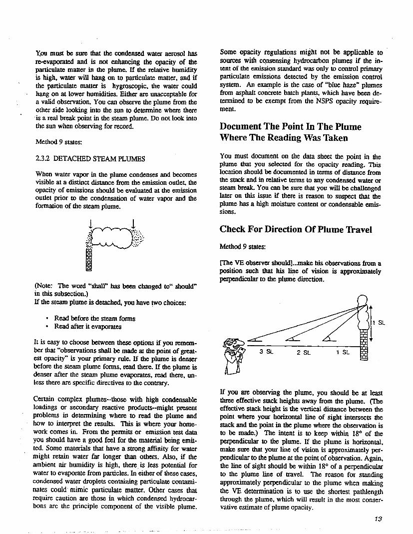
Method 22 is used in conjunction with emission standands or work practices in which 11p visible emissions is the stated goal. This is frequently the case with fugitive emission sources or sources with toxic emissions. Method 22 differs from Method 9 in that it is qualitative rather than quantitative. Method 22 indicates only the presence or absence of an emission rather than the opacity value. Thus, many of the provisions of Method 9 that enhance the accuracy of the opacity measurement are not necessary in Method 22 determinations. Method 22 does not require that the sun be the light source or that you stand with the sun at your back In fact, for reading asbestos emissions regulated under NESHAP Subpart M, you are directed to look toward the light source to improve your ability to see the .emission. Under Method 22, the duration of the emission is accurately measured using a stop watch. Table 2 on the following page compares major features of Method 9 and Method 22.

Later field studies have shown slightly higher observation errors, but they are still within the 7.5~percent opacity measurement error at two confidence intervals. These

6

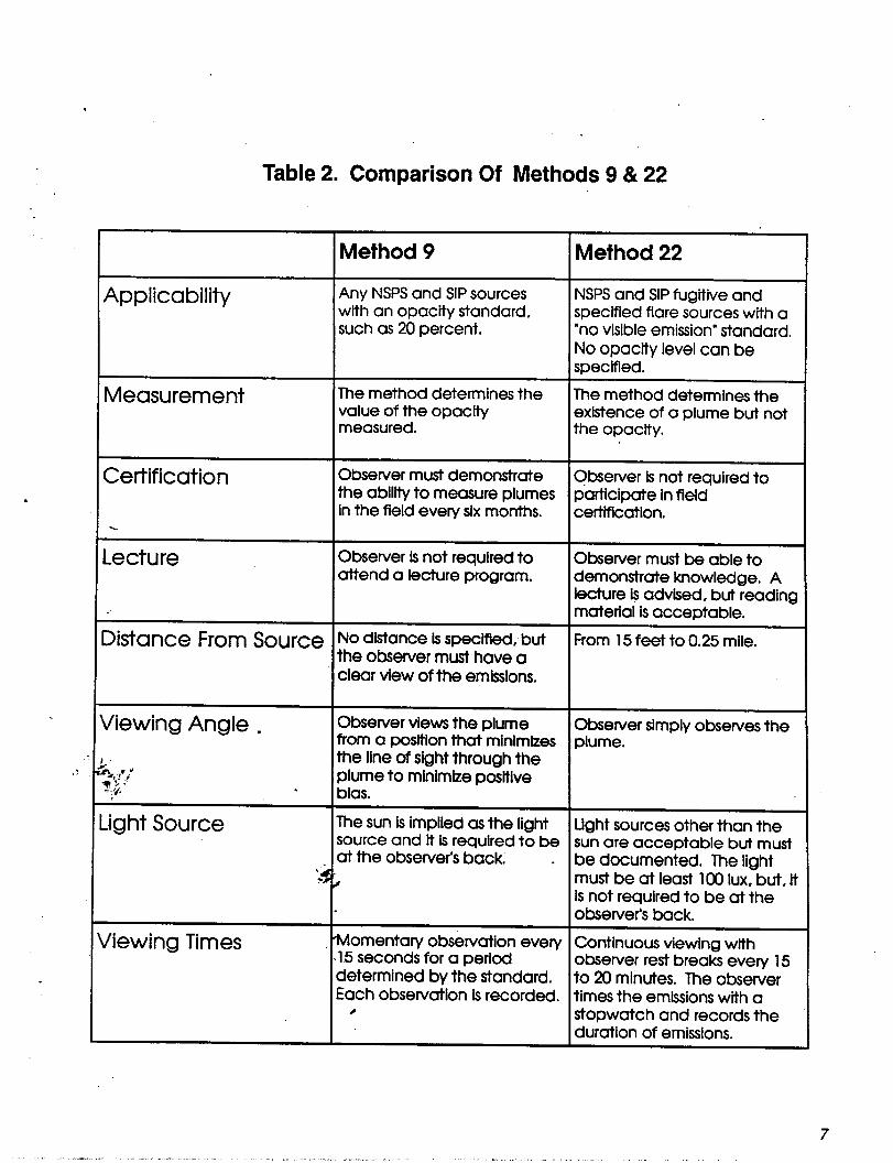
Table 2. Comparison Of Methods 9 & 22

Applicability

Measurement

Method 9 Method 22

Any NSPS and SIP sources NSPS and SIP fugitive and with an opacity standard, specified flare sources with a such as 20 percent. ‘no visible emission’ standard.

No opacity level can be specified.

The method determines the The method determines the value of the opacity existence of a plume but not measured. the opacity.

Certification Observer must demonstrate the ability to measure plumes

qbserver ls not required to participate in field

in the field every six months. certification.

Lecture Observer is not required to Observer must be able to attend a lecture program. demonstrate knowledge. A

lecture is advised, but reading i material is acceptable.

Distance From Source ;edi~i;;riss.sxzh~,~ut From 15 feet to 0.25 mile.

clear view of the emissions.

Viewing Angle . Observer views the plume from a position that minimizes

Observer simply observes the plume.

k’ the line of sight through the +g; 9 ‘I : plume to minimize positive . -‘,: . bias.

Light Source

diewing Times

The sun is implied as the light Light sources other than the source and it is required to be

. at the observer’s back sun are acceptable but must

. be documented. The light must be at least 100 lux. but, ti is not required to be at the observer’s back.

‘Momentary obs&vation every Continuous viewing with -1.5 seconds for a period determined by the standard.

observer rest breaks every 15 to 20 minutes. The observer

Each observation is recorded. times the emissions with a , stopwatch and records the

duration of emissions.

7

Records Review

Standard Visible Emission Inspection

The standard VE observation starts with a review of the source records on the emission point of interest. This initial review of the records can prevent considerable confusion and lost tune in the field. You might not have the opportunity to make the review before the inspection, in which case the documentation should be completed after the review. The following paragraphs describe the items that should be checked.

The regulatory requirements and compliance status of the emission point are critical. To use the correct measurement method and the correct data-reduction technique, you must know which regulations apply.

You must determine whether the emission point is regulated under federal New Source Performance Standards (NSPS), the State Implementation Plan (SIP), special permit conditions, or compliance order/agreement conditions. You must check each potentially applicable regulation: if you do not, you might use the wrong test method or data-reduction method. You cannot rely entirely on the Method 9 procedure in Appendix A of 4OCFR Part 60. If the source is NSPS- regulated, special procedures or other modifications could be included in the emission standard for a specific source category.

SIP regulations often stipulate procedures that vary from Method 9, eveh though Method 9 or a similiar method is referenced in the SIP regulation. These variances could be in the observation procedures, in certification requirements,.or in the data-reduction technique. The Ksec- ond opacity values could be reported as time duration (time aggregation), or as shorter or longer averages than 6 minutes, or as the number of individual values above a “cap” (not to exceed rules). You should check the applicability of the standard to the specific process unit, and you should also check for exempt operating conditions, such as start-up, malfunction, and shutdown.

Another source of information regarding the applicable standards as well as observation and data reduction procedures for a source is the operating permit. Special con-

ditions are often placed in the permit. Also, any negoti- . ated compliance orders or agreements pertaining to the source may contain references to opacity standards and compliance methods or other written procedures.

Previous observations that have been made by the source, your agency, or another agency should be reviewed. Check for photographs of the source, and make copies to take on the evaluation to help in identifying emission points, performing observations in a consistent manner, and documenting changes in plant equipment.

Review any available videotape to get a feel for the site and the emissions. VF Observation Forms from previous inspections should be evaluated to determine whether steam plumes or other unusual conditions exist. Check inspection reports for viewing conditions or locations.

Maps and plot plans are often found in the agency source file, which will help you in determining good obsewa- tion positions and their access. Time can be saved by using the maps and plot plans and calculating the sun’s position at different times of the day.

Emission test reports are a good source of data on the stack height, source type, and compliance status with other regulations such as mass emissions regulations. Stack temperature and moisture content can be used to determine whether a steam plume could potentially be present on the day of your observation using the technique described in the EPA Quality Assurance Hand- book, Volume III, Section 3.12.

Some emission reports have data on particle size distribution. Thii information is useful when observing a plume. Small Particles impart a bluish haze to a plume, because the particles scatter blue light preferentially. The test data might reveal whether there are condensable emissions in the gas stream. This information is helpful in determining whether any residual plume is due to, yater or to a complex plume reaction.

Stack test reports usually contain descriptions of control equipment and their operating conditions. This information is useful in determining whether there is potential for a water condensation plume to form

8

Lastly, fill in a sample VE Observation Form with the data that you have collected so that you have a ready reference when you go into the field. It is also useful to copy a map onto the back of the field forms you plan to use to help locate or verify the exact observation point.

Reverse Observations

Sometimes, you must make VE observations before a formal record review. Impromptu observations are often necessary when an opacity event is discovered. In this case, you will not have time for an extensive pre-inspection data review. Document what you can determine accurately in the field and complete the documentation as soon as possible after the observation. Visible emissions records used in court are treated as evidence under the principle of past recollection recorded. This means that you wrote it down while it was stiII fresh in your mind. If you must change an entry due to new knowledge obtained in the file review:

1. Draw a thin line through the error WITHOUT OBLITERATING IT.

2. Write the correction above it in ink. 3. Initial and date the change.

Equipment

Method 9 does not contain any special requirements or specifications for equipment or supfilies; however, certain equipment is necessary to conduct a valid observation that will withstand the rigors of litigation. Other equipment, though optional, can make the collection of high-quality data easier. This section gives specifications, criteria or design features for the recommended basic VE equipment.

Clipboard And Accessories

You should have a clipboard, several black ballpoint pens (medium point), several large rubber bands, and a s&i- cient number of VE Observation Forms to document any expected and unexpected observations. Use black ballpoint pens so that completed forms can be copied and still remain legible over several reproduction generations. Rubber bands hold the data form flat on the clipboard under windy conditions and hold other papers and blank forms on the back of the clipboard. Use observation forms that meet EPA Method 9 requirements. Sample forms that have been extensively field tested are provided in Appendix A.

Timer

During a VE observation, it is necessary to time the 15 second intervals between opacity readings. You have a choice between using a watch or dedicated timer. The best practice is to attach two dedicated timers to your clipboard. Liquidcrystal-display timers are preferred because of their accuracy and readability. Use one timer to determine the start and stop times of the observation and the other timer to provide a continuous display of time to the nearest second You can set most stick-on timers to run from 1 to 60 seconds repeatedly. A timer with a beeper that sounds every 15 seconds is recommended for use in some industrial locations, because you can then pay attention to your surroundings and your safety and not the timer.

Compass

A compass ia needed to determine the direction of the emission point from the spot where you stand to obsesve the plume and to determine the wind direction at the some. Select a compass that you can read to the nearest 2’. The compass should be jewel-mounted and Iiquid- filled to dampen the needle’s swing. Map-reading com- passes are excellent for this purpose. Because you must take the magnetic declination for your area into account when you take the reading, you should consider invest- ing in a compass that allows presetting the declination.

9

Topographic Maps

United States Geological Survey (USGS) 7.5-minute to- pological maps are a practical necessity for serious opacity work From these maps you can determine your exact location, true north, distances, access roads, latitude, lon- gitude, magnetic declination, relative ground height, and background features. You also can use these maps to calibrate rangeflnders. If you am planning an inspection, photocopy the section of the map that shows the facility on the back of your observation form. Laminate the full- sized map for field use and to allow for temporary mark- ing with dry erasable pens.

Rangefinder

If you do not have a topographic map of the area, you will need a rangefinder. Even with a map, a rangefinder is useful in field work. The two types in general use are the split-image and the stadiomehic rangefmders. The split-image type uses the technique of superimposing one image over another to determine the distance. ‘Ihe most useful models for most opacity work have a maximum range of about 1,000 yards. To use the stadiometric rangefinder, you must know the height or width of an object at the same distance as the object of interest. Stadiometric rangefinders are lighter and more compact than split-image rangefinders. Split-image rangefinders, although inherently more accurate, are more likely to become uncalibrated if bumped during transport. ‘Ihe accuracy of either type of rangefinder should be checked on receipt and periodically thereafter with targets at known distances of approximately 1QO meters and 1,000 meters. Any rangefinder must be accurate to within 10 percent of the measurement distance.

Clinometer .

You will need a clinometric &vice for determining the vertical viewing angle. For visible emission observation purposes, it should be accurate within 3O. Many suitable devices are available in a wide range of prices, including Abbney levels, pendulum clinometers, and sextants. Abbney levels use a bubble in a curved tube to determine the angle with an accuracy of lo to 2”. ‘Ihe pendulum clinometer is the cheapest and has an accmacjl of about 2’ when used properly. It consists of a protractor and a plum bob. A sextant is very accurate but more expensive, and you will need to know the position of the actual horizon.

Sling Psychrometer -

If there is a potential for the formation of a condensed water droplet “steam” plume, you will need a sling psychrometer to determine the temperature and relative humidity of the atmosphere. The sling psychrometer consists of two thermometers. accurate to OST, mounted on a sturdy assembly attached to a chain or strap. One thermometer has a wettable cotton wick surrounding the bulb. Thermometer accuracy should be checked by placing the bulbs in a deionized ice water bath at OOC. Electronic models that use newly developed solid state sensors are also available and do not have to be slung. Electronic models are simpler to use but require tedious periodic calibration using standard salt solutions.

Sling Psychrometer

q i .

Dry Bulb

10

Binoculars

Binoculars are helpful for identifying stacks, searching the area for emissions and interferences, and helping to characterize the behavior and composition of the plume. Binoculars are designated by two numbers, such as 7 x 35. The frost number is the magnification and the second is the field of view. Seiect binoculars with a magnification of 8 or 10 (8 x 50 and 10 x 50 are standard designations). The binoculars should have color-corrected coated lenses and a rectilinear field of view. Check the color correction by viewing a black and white pattern, such as a Ringelmann card, at a distance greater than 50 feet. You should see only black and white: no color rings or bands should be evident Test for rectilinear field of view by viewing a brick wall at a distance greater than 50 feet. There should be no pincushion or barrel distortion of the brick pattern. Plume observations for compliance purposes should not he made through binoculars unless you are certified with binoculars.

35 MM Camera And Accessories

Use a camera to document the presence of emissions before, during, and after the actual opacity determination and to document the presence or lack of interferences. Photographs document the specific stack that is under observation but do not document the exact opacity. Se- lect a 35mm camera with through-the-lens light meter- ing, a %acro” lens or a 250 to 350~mm telephoto lens, and a 6-diopter closeup lens (for photographing the photo logbook). A photo logbook is necessary .for proper documentation. An example of a photo log is provided in Appendix A of this maruraL Use only fresh color negative film with an ASA of approximately 100. You can get first-generation slides or prints from negatives. The first photograph is of the log, identifying the time, date, and source. Log each photograph when you take it, The last photograph is of the completed log. Instruct the pro- cessor not to cut the film or print roll so that you can refer to the photo log at the end of the roll to identify each photograph.

Video

Video is an excellent tool for opacity work Because of the wider tonal range of video, it does a better job of

reproducing the actual appearance of the plume than pho-. tography. In tetis of resohnion, video is poorer than film. The hest video systems for opacity work include High 8 and Super VHS. Each gives 400 Lines of resolution. Edited tapes have near broadcast quality and are excellent for research and court work Regular VHS or regular 8 resolution is poor and duplicates are even worse. Select the highest quality videotape available for your system. Set and use the automatic date and tune feature when taping, title each shot in the field, and narrate while taping. A sturdy tripod is as necessary as a good

camera.

Field Operations

Perimeter Survey

Before making your observations you need to determine the correct viewing position for the source beiig monitored, and you must also identify any potential interferences. You will need to select backgrounds, detexmme the wind direction, and determine the position of the sun relative to the source. You also should look for unlisted sources at this time. If you do not consider each of these items, the observation could be invalid.

Determine Sources

First, determine the sources of visible emissions at the facility and identify the specific source that you are go- ing to observe. Record the source identification on the field data sheet. Next identify any potential interferences near the source for example, other visible emission plumes from nearby sources, fugitive dusts from work activities in the line of sight or obstructing buildings. Lastly. identify any other sources that are unlisted but visible.

Determine The Position Of The Sun .

Method 9 states: The qualified observer shall stand at a distance sufficient to provide a clear view of the emissions with the sun oriented in the 140 sector to his back.

This means that a line’from the sun to the observer and a line from the observer to the observation point in the plume must form an angle of at least 110 degrees. This

77

will place the sun in the required cone-shaped 140 degree sector. The purpose of this rule is to prevent forward scattering of light transmitted in the plume. Forward scattering enhances the plume visibility and creates a positive bias in measurement results. In fact, every viewing requirement of the method is designed to prevent positive bias.

Use a compass to determine the position of the sun in terms of true north. Remember to correct the compass for the magnetic declination at the site which might be different from that at your office location. When you position yourself initially you will position the sun in a 140 degree sector to your back when you face the source. Use the sun location line on the form for this initial check

Now you must determine whether the vertical location of

the sun is acceptable. This is especially true under one or more of the following conditions:

l You are observing a talI stack l The sun is high overhead l You are observing the plume high in the sky

In the summer the sun can be as high as or higher than 60” in the sky during the solar noon (1 p.m.) at most locations in the United States. If this is the case and the plume observation point is only 15’ in the vertical, the combined vertical angle (from the observation point to the observer to the sun) will violate the vertical requirements because the total of the vertical plume angle and the vertical sun angle is at least 75’ (which is less than the 110’ specified minimum). Finally, the horizontal and vertical angles have a combined effect. If the sun is the sun is high overhead, or if,the observation point is high, or if the observation point is high and the sun is close to the edge of the acceptable position, the final angle will probably be unacceptable.

Determine The Point In The Plutie To Evaluate ’

Method 9 provides excellent guidance on the selection of the spot in the plume to observe. This guidance is presented in several sections and, unless the method is read in its entirety, the information can be confusing. The following extractions from Method 9 address what to consider in selecting the point in the plume for the observation.

Method 9 states:

2.3 OBSERVATIONS

Opacity observations shaU be made at the point of greatest opacity in that portion of the plume where condensed water vapor is not present.

This is the first and most significant criterion. It has two elements that must be adhered to:

You must read opacity at the densest portion of the plume

There cannot be any condensed water vapor at the point of observation

If there is no condensed water droplet plume, you can read at the densest part of the plume. If there is a “steam” plume, sections 2.3.1 and 2.3.2 explain how to implement the rule.

Method 9 states:

2.3.1 ATTACHED STEAM PLUMES

When condensed water vapor is present within the plume as it emerges from the emission outlet, opacity observations shall be made beyond the point in the plume at which condensed water vapor is no longer visible. The observer shall record the approximate distance from the emission outlet to the point in the plume at which the observations are made.

Read Here I

72

You must be sure that the condensed water aerosol has reevapomted and is not enhancing the opacity of the particulate matter in the plume. If the relative humidity is high, water will hang on to particulate matter, and if the particulate matter is hygroscopic, the water could

. hang on at lower humidities. Either are unacceptable for a valid observation. You can observe the plume from the other side looking into the sun to determine where there ‘is a real break point in the steam plume. Do not look into the sun when observing for record.

Method 9 states:

2.32 DETACHED STEAM PLUMES

When water vapor in the plume condenses and becomes visible at a distinct distance from the emission outlet, the opacity of emissions should be evaluated at the emission outlet prior to the condensation of water vapor and the formation of the steam plume.

(Note: The word “shall” has been changed to“ should” in this subsection.) lf the steam plume is detached, you have two choices:

l Read before the steam forms l Read after it evaporates

It is easy to choose between these options if you remember that “observations shall be made at the point of greatest opacity” is your primary rule. If the plume is denser before the steam plume forms, read there. If the plume is denser after the steam plume evaporates, read there, unless there are specific directives to the contrary.

Certain complex plumes--those with high condensable loadings or secondary reactive products--might present problems in determining where to read the plume and how to interpret the results. This is where your home- work comes in. From the permits or emission test data you should have a good feel for the material being emitted. Some materials that have a strong affinity for water might retain water far longer than others. Also, if the ambient air humidity is high, there is less potential for water to evaporate from particles. Ln either of these cases, condensed water droplets containing particulate contami- nates could’ mimic particulate matter. Other cases that require caution are those in which condensed hydrocar- bons are the principle component of the visible plume.

Some opacity regulations might not be applicable to sources with consensing hydrocarbon plumes if the intent of the emission standard was only to control primary particulate emissions detected by the emission control system. An example is the case of “blue haze” plumes from asphalt concrete batch plant+. which have been determined to be exempt from the NSPS opacity requirement.

Document The Point In The Plume Where The Reading Was Taken

You must document on the data sheet the point in the plume that you selected for the opacity reading. This location should be documented in terms of distance from the stack and in relative terms to any condensed water or steam break You can be sure that you will be challenged later on this issue if there is reason to suspect that the plume has a high moisture content or condensable emissions.

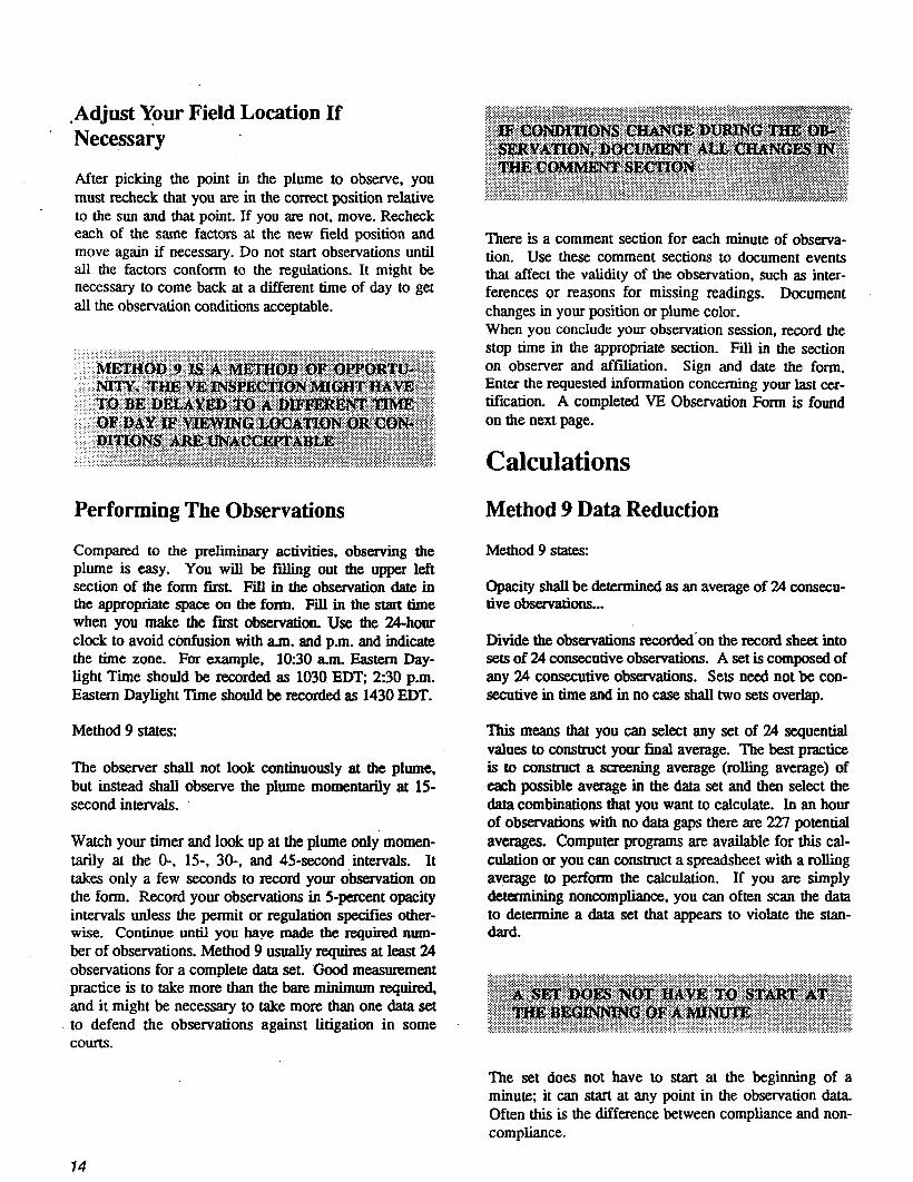
Check For Direction Of Plume wave1

Method 9 states:

IThe VE observer should]...make his observations from a position such that his line of vision is approximately perpendicular to the plume direction.

SL

If you are observing the plume, you should be at least three effective stack heights away from the plume. (The effective stack height is the vertical distance between the point where your horizontal line of sight intersects the stack and the point in the plume where the observation is to be made.) The intent is to keep within 18” of the perpendicular to the plume. If the plume is horizontal, make sure that your line of vision is approximately perpendicular to the plume at the point of observation. Again, the line of sight should be within 18O of a perpendicular to the plume line of travel. The reason for standing approximately perpendicular to the plume when making the VE determination is to use the shortest pathlength through the plume, which will result in the most conser- vative estimate of plume opacity.

73

,Adjust Your Field Location If Necessary .

After picking the point in the plume to observe, you must recheck that you are in the correct position relative to the sun and that point. If you ate not, move. Recheck each of the same factors at the new field position and move again if necessary. Do not start observations until all the factors conform to the regulations. It might be necessary to come back at a different time of day to get all the observation conditions acceptable.

Performing The Observations

Compared to the preliminary activities, observing the plume is easy. You will be filling out the upper left section of the form fmt. Fill in the observation date in the appropriate space on the form. Fii in the start time when you make the fmt observation. Use the H-hour clock to avoid confusion with am. and p.m. and indicate the time zone. For example, 10~30 am. Eastern Day- light Time should be recorded as 1030 EDT, 230 p.m. Eastern Daylight Time should be recorded as 1430 EDT.

Method 9 states:

Tbe observer shall not look continuously at the plume, but instead shall observe the plume momentarily at 15 second intervals.

Watch your timer and look up at the plume only momentarily at the 0-, 15, 30-, and 45second intervals. It takes only a few seconds to record your observation on the form. Record your observations in j-percent opacity intervals unless the permit or regulation specifies otherwise. Continue until you have made the required number of observations. Method 9 usually requires at least 24 observations for a complete data set. Good measurement practice is to take more than the bare minimum required, and it might be necessary to take more than one data set to defend the observations against litigation in some courts.

There is a comment section for each minute of observation. Use these comment sections to document events that affect the validity of the observation, such as interferences or reasons for missing readings. Document changes in your position or plume color. When you conclude your observation session, record the stop time in the appropriate section. Fill in the section on observer and affiliation. Sign and date the form. Enter the requested information concerning your last certification. A completed VE Observation Form is found on the next Rage.

Calculations

Method 9 Data Reduction

Method 9 states:

Opacity shaIl be determined as an average of %I consecutive observations...

Divide the observations recorded’on the record sheet into sets of 2A consecutive observations. A set is composed of auy 24 consecutive observations. Sets need not be consecutive in time and in no case shall two sets overlap.

This means that you can select any set of 24 sequential values to construct your final average. The best practice is to construct a screening average (rolling average) of each possible average in the data set and then select the data combinations that you want to calculate. In an hour of observations with no dam gaps there ate 227 potential averages. Computer programs are available for this calculation or you can construct a spreadsheet with a rolling average to perform the calculation. If you are simply determining noncompliance, you can often scan the data to determine a data set that appears to violate the standard.

The set does not have to start at the beginning of a minute; it can start at any point in the observation data. Often this is the difference between compliance and noncompliance.

74

VISIBLE EMISSION OBSERVATION FORM

7 20 35 25 35

8 30 30 30 25

9 30 35 40 30

10 25 20 15 30

11 40 35 40 35

13 30 1 25 [ 20 1 30 1 1

14 25 20 t5 15

15 - - 25 35 /iPEflNg P?ffME

16 30 I30 I30 125 1 I

t 10 120 135 125 135 1

= I25 1 20 i 15 1 I

Method 9 states:

For each set of 24 observations, calculate the average by summing the opacity of the 24 observations and dividing this sum by 24.

A simple mean is calculated for each data set and each mean is compared to the standard. If any correction is made for pathlength, it must be made before calculating the average.

Method 9 states:

If an applicable standard specifies an averaging time requiring more than 24 observations, calculate the average for aU observations made during the specified time pe-

. liod.

Federal &ndards and SIP opacity regulations sometimes contain averaging times other than 6 minutes. EPA’s policy is that if the SIP regulation does not clearly specify an averaging time or other data-reduction technique, the 6-minute--average calculations should be used. EPA is currently in the process of providing additional methods to cover alternative averaging times.

Time-Aggregation Standards

Time-aggregation standards are generaly stated in terms of an opacity limit that is not to be exceeded for more than a given time limit, such as 3 minutes, over a total period, &$@s 1 hour. The usual technique is to count the numb&of observations that violate’the standard during the observation period. Multiply the number of vi+ lations by 15 seconds to get the total number of seconds in violation and divide by 60 to get the number of minutes of violation. Compare the answer to?* standard. EPA is in the process of promulgating metho& that will allow for time-aggregation calculations. -

Data Review . ‘1

Field Data Check ,

Before you leave the field, look over the form carefully. Start at the bottom right-hand section and work your way up, following the form backwards. Make sure that each section is* either filled out correctly or is left blank on purpose. AU entries should be legible. Remember, this is

the first-generation copy and all subsequent copies will be of lower print quality. As stated earlier in thii manual, the visible emission observation form is usually intro- duced as evidence in enforcement litigation under the principle of “past recollection recorded.” This means that you made entries on the form ,while they were fresh in your mind A five-minute review at this time can Save hours later.

Complete The Form

As soon as possible, gather the missing information and complete the form. Do not sign the form until you have completed all entries you intend to complete.

Method 9 warns:

-are recorded on a field data sheet at the time opacity readings are initiated and completed.

Any additional enties made after you sign the form must be dated and initialed. Failure to document changes properly makes the observations subject to challenge. Even the markout might have to be explained in a deposition or in court.

Quality Assurance Audit

If the form is used as proof of compliance or of violation in a permit application or of agency enforcement action, a third party should review the document in detail. The following sections describe the elements of a minimal audit.

After each item on the form is checked, you should compare related data items for consistency. For example, check if:

l The wind direction arrow in the sketch agrees with the wind direction recorded in the text section of the form.

l The final signature date is consistent with the observation date.

l The time of day is consistent with the sun position.

76

Compare the date of the observation at the top of the form with the date of the certification at the bottom of

. the form. The observation date must be after the certification but no more than 6 months after.

Method 9 has specific requirements for recording information regarding the emission source or point observed and the field conditions at the time of the observation. Check to see whether the following information is pro vided on the VE Observation Form:

.

. . . . . . . .

. . .

.

Name of the plant Facility and emission point location. Type of facility. Observer’s name and affiliation. . - Date and time of observation. Estimated distance to the emission location. Approximate wind direction. Estimatedwind- Description of the sky conditions (presence and color of clouds). Plume background. Sketch of sun, source, and observer positions. Distance from the emissiin outlet to the point in the plume at which the observations are made. 24 observations (unless other criteria exist).

If any of these items is missing, it wiI.l be pointed out in a deposition, or in a motion before the court, or to the judge when you are on the wimess stand.

Compliance with sun angle regulations is one of the most difficult items to audit accuxately because of inadequate documentation. The angle cteated by the line of sight of the observer and the line from the sun to the observer must be at least 110”. This places the sun in the 1409 cone-shaped sector to the observer’s back Sun angle has both horizontal and vertical components, and both must be reviewed.

HorizontaI sun angle is the easiest to check. Com- pare the direction to the measurement point with the position of the sun at that time of day. If the sun location line on the suggested form is used, this should be easy. If the line looks right, you must still check it against the north arrow in the sketch. You can check the sun location for accuracy using the US Naval Observatory ICE program or solar tables. If all these records are reasonable, you can calculate the horixontal angle. The angle must be at least 118. Next, check the vertical sun angle. Add the vertical angle of the observer’s line of sight to the vertical line of sight to the sun. The total of these two angles must be less than 70”.

Lastly, both horizontal and vertical angles must be combined to get the resultant angle. This requires solid trigonometry. Commercial computer programs exist that perform the task. As a general rule, if the total vertical angle is less than W and the horizontal angle is above 1300, the resultant angle should be acceptable. Otherwise, the observation is suspect,.

fn order to assure that the sight line was approximately perpendicular to the direction of plume travel, the slant angle should be less than 18’. Use the distauce from the stack and the effective stack height to determine the angle. If the plume was horixontal at the point of observation, check the sketch for the direction of plume travel. Then check to see if the plume direction and wind direction are reasonable.

Check to see that the plume -was observed along a line of sight perpendicular to the long axis of the vent if the vent is not circular. This is important when observing fugitive emissions. Sources such as stor- age piles. dusty roads, roof monitors, and ships’ holds are difficult to observe properly because of this

requirement. In many cases you must reach a compro- mise between the axis of the source and the axis of the plume. If the reading is not made from a position nearly perpendicular to the plume, you should look at the final opacity and determine whether correcting the data for pathlength will still give the same final result in terms of compliance status.

Were observations made at 1%second intervals or in compliance with the applicable regulations?

Were a minimum number of observations made with no data gaps? If data gaps exist, am they explained? If an average was calculated with a data gap, what value was assigned to the dam gap? What is the reason for selecting the value?

Check for possible interferences. Obstacles in the line of sight or other emission plumes in front of or behind the plume being monitored create interferences that must be avoided or noted on the data form. Review the sketch for other vents, stacks, or sources of fugitive emissions that might cross the line of sight or co-mingle with the plume being evaluated and create a positive bii in the observations. Compare any photographs to the sketch. The sketch should indicate the backgrounds and their relative distances. If mountains or other distant objects are used as a reading background, check if haxe is indicated in the background section. This will potentially create a negative bias in the opacity readings. Also, note in the comments section beside the observation whether interferences were reported. Lastly. check the additional information section and the data section for comments regarding haze or other interferences.

Was the emission observed at a point where there was no condensed water? If the form indicates the presence of a steam plume, pay special attention to the point in the plume where the observation was made. Does it make sense in relation to instructions given in sections 2.3, 2.3.1, and 2.3.2 of the Method 9? Check the ambient temperature and relative humidity, if available. If the temperature is low or if the relative humidity is high (over 70 percent), consider the possibility of a steam plume that does not evaporate easily. If the data are available, model the steam plume using the technique in EPA Quality Assurance Handbook, Volume III, Section 3.12. When you use this model you must recognize that

The charts were developed from steam tables to represent the conditions in an ideal closed system, and the atmosphere is not an ideal closed system.

The tables do not consider the presence of particulate matter or condensation nuclei.

The temperature of the emission gases is an average of at least a onehour emission test and does not necessarily represent a steady-state condition in the stack.

The moisture content entered into the calculation is an average of at least one hour and might not be representative of the plume conditions over a shorter time frame. The chart does not recognize that the plume might not be uniform in moisture concentration and that some portions of the plume might be at supersaturation.

The tables do not consider the presence of hygro scopic particulate matter that could attract and hold onto water by lowering its vapor pressnre.

The chart is best used by constructing a line with an error band that recognizes the associated error in measurement of each of the input parameters. It should be assumed that no water plume forms only if the error band does not approach the dewpoint.

Are the calcuhitions in compliance with the mgnhttion? Does the regulation require averaging over a time period other than 6 minutes? Does it require time aggregation? Is the math correct? Was the highest average determined? Is there data showing noncompliance in excess of the regulation in terms of opacity and time?

18

Verify that no interferences or extenuating circumstances existed during the observation that would make the opacity values not representative of actual conditions or otherwise invalidate the observation.

Depending upon the potential use of the form, it may be wise to have an additional third party audit the form. After completing the second audit, compare the results of the two independent audits and resolve any outstanding difficulties.

. .

. .

.

,

C

Further Readings .

Field Observation Procedures:

Quality Assurance Handbook for Air Pollution Measurement Systems: Vol. III Stationary source Specific Methods, Section 3.12 - Method 9 Visible Determination of Opacity of Emissions from Stationary Sources, EPA 600/4-77- 027b. February 1984.

Guidelines for Evaluation of Visible Emissions: Certification, Field Procedures, Legal Aspects and Background Materials, EPA 340/l-75-007, April 1975.

Guide to Effective Inspection Reports for Air Pollution Violations, EPA 340/l-85-019, September 1985.

Instructions for Use of the VE Observations Form, EPA 340/l-86-017.

Observer Raining and Certification:

Self-Audit Guide for Visible Emission Training and Certification Programs, EPA 455/R-92-005.

Technical Assistance Document Quality Assurance Guideline for Visible Emission Training Schools, EPA 600/4- 83-011.

Course 325 - Visible Emission Evaluation: Student Manual, EPA 455/B-93-01 la, Jauuary 1994.

Opacity Evaluation Methods:

Optical Properties and Visual Effects of Smoke&a& Plumes, AP-30, Revised May 1972.

Evaluation and Cohborative Study of Method for Visual Determination of Opacity of Emissions from Stationary Sources, EPA 650/4-75-009, January 1975.

Measwement of the Opacity and Mass Concenlxation of Particulate Emissions by Transmissometry, EPA 650/Z-74- 128, November 1974.

20

Appendix A

Forms

./

_*j _ _ , , . . , , - . 4 . . . -L ^ _- . _*.~ _ , . . - . .__; . . - a / , _I ,_” . Xr. . . ) . ^ “ - . I . , . _ .

VISIBLE EMISSION C IBSERVATION F*“” ’ 1

5 I

6

1 I 1

EMISSIONS I

SCWRCEIAYMSKEI-CH uwwwJnnARwmr

X Ebassohm 0

I SUNLOUKNUNE

10

11

12 ’

I

P

24

25

26

FUGITIVE OR SMOKE EMISSION INSPECTION OUTDOOR LOCATION

Company Observer Location tf$iation Company Rep.

Sky Conditions Wind Direction Precipitation Wind Speed

Industry Process Unit

Sketch process unit: indicate observer position relative to source and sun, indicate potential emission points and/or actual emission points.

c

OBSERVATIONS Observation Accumulated

Clock period emission

time duration, time, Begin Observation min:sec min:sec

End Observation

Figure 22-l

FUGITIVE EMI’SSION INSPECTION INDOOR LOCATION

Company Observer

Location Affiliation

Company Rep. Date


Light type(fluorescent,incandescent,natural)

Light location(overhead,behind observr etc)

Illuminance(lux or footcandles)

Sketch process unit: Indicate observer position relative to.source; indicate potential emission points and/or actual emission points. .-

_I

OBSERVATIONS Observation Accumulated Clock period emission

. time duration, time, - Begin Observation mimsec min:sec

4* : CF~. ,* ,’ “Jj,’

‘3;

f

,-

End Observation

Figure 22-2

Photo Log

# Time/Date Subject

1.

2.

3.

4.

5.

6.

7

8.

9.

,lO. ./

11.

12.

Appendix B

Method 9 - Visual Determination of the Opacity of Emissions from Stationary Sources

. . . . , , . , , . s , . . . _ . . “ , . c . * , a . “ . ” ,W,^ _“ I . . - . * . “ . ^ . , , . . / , , . . ,

llarotiuction

(a) Many stationary sources discharge visible emissions into the atmosphere; these emissions are usually in the shape of a plume. This method involves the detetmination of plume opacity by qualified observers. The methods includes proce dues for the training and certification of obsetv- en and procedures to be used in the field for determination of plume opacity.

01) The appeamnce of a plume as viewed by an observer depends upon a number of variables, some of which may be controllable in the field Variables which can be controlled to an extent to which they no longer exert a significant influence upon plume appearance include: angle of the ob server with respect to the plume; angle of the ob- serverwithrespecttothestnupointofobserWion of attached and detached steam plume: and angle of the observer with respect to a plume emitted from a rectangular stack with a large length to width ratio. The method includes specific criteria applicable to these variables

(c) other variables which may not be conttouable in the’ field are lm and color contrast between the plume and the ba&gmu& against which tire plume is viewed. These variables exert illliIlflU~UpOUthe vofaphnneas viewedbyanobserverandcanaEecttheabilityof the observer to assign accmatelyopacityvahlesto the observed plume. Studies of the theory of plume opacity and field studies have de.rnonsuamd that a plume is most visible and presents the greatest apparent opacity when viewed against a co&g background Accoukngly. the opacity of a plume viewed under conditions where a contrasting background is present can be assigned with the greatest degree of accuracy. However, thepotentialforapositiveenwrisalsothegreatest when a plume is viewed under such contrasung conditions. Under. conditions fnesenting a less contmsting background, the apparent opacity of a phrmeislessandapproachesxeroasthecolorand luminescence contrast decmase toward zero. As a result, significant negative bias and negative er- rurscanbemadewhenapl~eisviewedunder less contrasting conditions. A negative bias de- cmasesratherthanincreases the possibiity that a phUt0peratorWillbe irkcomctly cited for a violation of opacity standards as a result of observer error.

B-2

(d) Studies have been undertaken to determine the magnitude of positive errors made by qualified observers while reading plumes under contrasting conditions and using the pmcedums set forth in this method. The results of these studies (field trials) which involve a total of 769 sets of 25 readings each are as follows: (1) For black plumes (133 sets at a smoke generator), 100 percent of the sets were read with a positive error of less than 75 percent opacity; 99 percent were read with a positive error of less than 5 percent opacity. (Note: For a set, positive error = average opacity detemiued by observers’ 25 observations -average opacity determined from uansm&ometer’s 25 record- ings.)

(2) For white plumes (170 sets at a smoke generator, 168 sets at a coal-tied power plant, 298 sets at a sulfuric acid plant>, 99 percent of the sets were read with a positive error of less than 7.5 percent opacity: 95~tweFereadwithapositiveerroroflessthan 5 percent opacity.

(e) The positive observational error associated with an average of twenty-five readings is therefore estab lished. lIteaccmacyofthemethodmustbetakeninto account when determining possible violations of apph- cable opacity standa&.

L Principle And Applicability

Ll Principle. The opacity of emissions !iom station- arysourcesisdemrminedvisuallybyaqualifiedob- sel-va.

L2 Applicability. This method is applicable for ti. determmation of the opacity of emissions from stationary sources pursuant to fj 60.11(b) and for visually deteaminhg opacity of emissions.

2. Procedures lbeobserverquaIifiedm accordance with section 3 of this method shall use the following procedutes for vi- sualiy determhing theopacity of emissions.

2.1 Position. The qualikd observer&all standata distance sufficient to provide a clear view of the emissions with the sun oriented in the 140” sector to his back. Consistent with maintaining the above require merit, the observer shall, as much as possible, make his observations from a position such that his line of vision is apptoximaMy perpendicular to the plume direction and, when observing opacity of emissions

. . - . - , . - . . 1 . . “ I , . , A*- ^ 1 ~,1, - ” . / / . ._

.

,

,

fmm rectangular outlets (e.g.* roof monitols. open baghouses, noncircular stacks), appnximately perpendicular to the longer axis of the outlet. The observer’s line of sight should not include more than one plume at a time when multiple stacks are involved, and in any case the observer should make his observations with his line of sight perpendicular to the longer axis of such a set of multiple stacks (e.g., stub stacks on baghouses).

22 Field Records. ‘Ihe observer shah record the name of the plant. emission location, facility type, observer’s name and affiion, a sketch of the ob server’s position relative to the so-, and the date on a field data sheet (Figure 9-l). The time, estimated distance to the emission location approximate wind direction, estimated wind speed, deXziption of the sky condition (presence and color of clouds), and plume background are mcorded on a field data sheet at the time opacity readings are initiated and completed.

23 observations. opacityobtxxwionsshallbe madeatthepointofgreakstopacityinthatportion oftheplumewhetecondensedwatervaporisnot pnxentm The observer shah not look continuously at the plume but instead shah observe the plume me mentarily at 1QecondintezMs.

23.1 At&ached Steam Plumes. When condensed watervaporisptesentwithintheplumeasitemerg- es fkom the emission outlet, opacity observatiaos shall be made beyond the point in the plume at which condensed water vapor is no longer visible. ne0bserv~shallrec0rdtheapplroximatedistance fmm the emission outlet to the point in the plume at which the observations ate made.

2.32 Detached ste!am Plume. when water vapor in the plume condenses and becomes visible at a distinct distance from the emission outlet, the opaci- tyofemissionsshouldbeevahuuedattheeznission outlet prior to the condensation of water vapor and the fotmation of the steam plume. -

2.4 Recording Observations. Opacity obscrva- tionsshallbemconiedtotheneamst5percentat 15-second intervals on .an observational record sheet. (See Figure 9-2 for an example.) A mini- mutn of 24 observations shall be tecora Each momentary observation mcorded shah be deemed to

represent the average opacity of emissions for a 15- second period.

25 Data Reduction. Opacity shaIl be deuzmined as an average of 24 consecutive obsetvations recorded at 15second intervals. Divide the observations recordd on the record sheet into sets of 24 consecutive observations. A set is composed of any 24 consecutive observations Sets need not be consecutive in time and in no case shall two sets overlap. For each set of 24 observations, calculate he average by summing the opacity of the 24 observations and di- vidingthissumby%. Ifanappkablestatxkd specifies an averaging time requiring more than 24 obsemtions, calculate the average for all observations made during the specified time pdxL Record the average opacity on a record sheet. (See Figure 9- 1 for an example.)

3. Qdfication and Testing

3.1 Certification Requirements, To receive ccrtifi- cationasaqualitiedobsesver,acandidatemustbe testedanddemonscrate theabilitytoassignopacity readingsin5~mt incrementsto2sdifferent black plumes and 25 different white plumes, with an enornottoexceed15petcentopacityonanyone reading and average error not to exceed 7.5 petcent opacityin~category.candidalesshaube~ accmlingtotheproceduFesdescribedinSection3.2 Smoke generatots used pursuant to Section 3.2 shall be equipped with a smoke meter which meets the mquirements of Section 33. The certification shah bevalidforaperiodof6months,atwhichtimeme quaUc&onproceduremustbempeatedbyanyob- server in order to retain certification.

32 Certification Procedure. The certi!?cation test consists of showing the candidate a complete run of 50 plumes-25 black phunes and 25 white plumes- gcxmated by a smoke genemtor. Phnnes within each setof25blackand25whitenmsshallbepmsemed in tandem order. The candidate assigns an opacity valuetoeachplumeandrecordsh.isobservaGonona suitable form. At the completion of each run of 50 madings,thescoreofthecandidateisdetenn&d. If a candidate fails to qualify, the complete run of 50 readings must be mpeated in any retest. The smoke testmaybeadministeredaspattofasmokeschoolor tminingprognunandmaybeprecededbyuainingor . . . -on runs of the smoke generator during which candidates are shown black and white plumes of hewn opacity.

33 Smoke Generator Specifications. Any smoke generator used for the purposes of Section 3.2 shall be equipped with. a smoke meter in- stalled to measure opacity across the diameter of the smoke generator stack. The smoke meter output shall display in-stack opacity based upon a pathlength equal to the stack exit diameter, on a full 0 to 100 percent chart recorder scale. The smoke meter optical design and performance shall meet the specifications shown in Table 9-1. The smoke meter shah be calibrated as prescribed in Section 3.3.1 prior to the conduct of each smoke reading test At the completion of each test, the zeroandspandriftshallbecheckedandifthe drift exceeds *I pcem opacity, the condition shall be ccmcti prior to conducting any subsequent test runs. The smoke meter shall be dernon- strated at the time of insWati0~ to meet the specifications listed in Table 9-l. This demonstration shall be repeated following any subsequent repair or replacement of the photocell or associated electronic circuitry including the chart recorder or output meter, or every 6 months, whichever occurs first.

33.1 Calibration. The smoke meter is calhat- exl after allowing a minimum of 30 minutes warmupbyahematelyproduciisimulatedopaci- tyofOpercentand1OOpement. Whenstable responseatOpercentor1OOpercentisnotedthe smoke meter is adjusted to produce an output of 0 percent or 100 percent, as appqniate. This cah- brationshallberqeateduntilstableOpementand lOOpementopacityvaluesmaybepmduc&by alternately switching the power to the fight source on and off while the smoke genemtor isnotm ducing smoke.

33.2 *Smoke Meter Evaluation. The smoke meter design and performance aretobeeval~ as follows:

333.1 Light Source. Verify from manufacturer’s data and from voltage measurem entsmadeat thelamp,asinstall~thatthelampisopemted within FY percent of the nominal rated voltage.

3333 Spectral Response of Photocell. Verify from manufacturer’s data that the photocell has a photopic reqonse; i.e., the spectral sensitivity of the cell shall closely approximate the standard spectral-luminosity in (b) of Table 9-1.

332.3 Angle of View. Check construction geometry to ensure that the total angle of view of the smoke plume, as seen by the photocell, does not exceed Ho. ThetotalangleofviewmaybecalculaMfrom:B=2 tan-’ (cU2L). where & = total angle of view: d = the sum of the photocell diameter + the diameter of the limiting aperture; and L = the distance from the photo cell to the limiting aperture. The limiting aperture is the point in the path behveen the photocell and the smoke plume where the angle of view is most restrict- ed In smoke generator smoke meters this is normally an orifice plate.

33.2.4 Angle of Projection. Check construction geometry to ensure that the total angle of projection of the lamp on the smoke plume does not exceed 15”. The total angle of projection may be calculated i%ortu I? = 2 tan’ (&2L), where fi = total angle of projection; d=thesumofthelengthofthelampfihunent+the diameterofthelimitingapertute;andL=thedistance from the lamp to the limiting aperture.

33.25 Calibration Error. Using neutraldensity fil- texsofknownopacity.checktheermrbehveenthe actualrlqNmseandthetheoletical~msponseof the smoke meter. This check is accmnplisbed by first calibratingthesmokemeteraccor&ngtoSection33.1 andtheninsmtingaseriesofthmeneunaMensityfil- ters of nominal opacity of 20.50, and 75 percent in the smoke meter pathlength. Filters calibrated within 2 percentshallbeused. Careshouldbetakenwhen insating the films to prevent stray light from affect- ing the meter. Make a total of five nonconsecutive readings for each filter. The maximum error on any cmereadingshallbe3percentopacity.

33.2.6 Zero and Span Drift. lkwmine the zero and span drift by calibrating and operating the smoke generator in a normal manner over a l-hour period. Thedriftismeasuredbycheckingthezen,andspanat theendofthispetiod.

33.2.7 Response Time. Determine the response time by producing the series of five simulated 0 percent and 100 percent opacity values and observing the time required to reach stable response. Opacity values of 0 ’ percent and 100 percent may be simulated by alternately switching the power to the fight source off and on while the smoke generator is not operating.

Table 41. Smoke Generator Design And Performance Specifications

Parameter Specification

a. Light source Incandescant lamp opexated at nominal rated voltage

b. Spectral response of Photopic (daylight spectral respcme of the human eye photocell -Citation 3)

c. Angle of view 15 l/2 maximum total angle

d. Angle of projection 15 l/2 maximum total angle

e. Calibration emr + 3 8 opacity, maximum

f. zemandspandlift +l%opacity,3Ominutes

g. Responsetime +5seumds . .

Bibliography

L Air Pollution control District Rules and Regulations. Ias Angeles Coun@ Air Pollution Cm&o1 District, Re8ulation IV, Pmhiiitim Rule 50.

i

2. Weisw Melvin I., F& operatons and Enforcemen t Ivlamal for Air, U.S. EmifoMlentaI Plmmion Agency, Reseat& Triangle Pa& NC, AFI’D-1100, August 1972, pp. 4.1436.

3. Conh EU., and Odishaw, I-I., Handbook of Physics, McGraw-Hill Co., New York, NY, 1958, Table 3.1, p. G-52.

.

.

Figure g-1. Record of Visual Determitiation of Opacity -I

Company I Location

Test No.

Date

Type Facility

Control Device

Hours of Observation

Observer

Observer Certification Date Observer Affiliation

Point of Emissions Height of Discharge Point

Wind Direction Wind Speed Ambient Temperature

Sky Conditions (clear, overcast, % clouds, etc.)

Plume Description Color Distance Visible

Other Information

SUMMARY OF AVERAGE OPACITY

Set Number Time

Start - End

Opacity Sum Average

I

Figure 9-2. Observatiqn Record Page of

Company . Observer

Location Type Facility

Test Number Point of Emissions

Seconds

Hr Min 0 15 30 45 0

I I I I

1 I I I I

2 3 4 5 6 7

I

12 13 14 15 16 17

18 l-9

Figure 9-2. Observation Record’ (continued)

Company

Location

Test Number

Page

0 bserver

Type Facility

Point of Emissions

Of

Seconds Steam Plume

(Check if applicable) Comments

- Appendix C

Method 22 - Visual Determination of Fugitive Emissions from Material Sources and Smoke Emissions from Flares

1. Introduction

1.1 ‘IIis method involves the visual determination of fugitive emissions, i.e., emissions not emitted directly from a process stack or duct. Fugitive emissions include emissions that (1) escape capture by process equipment exhaust hoods; (2) ate emitted during ma&al transfer, (3) are emitted from buildings housing material processing or handling equipment; and (4) are emitted directly from process equipment this method is usedalso to determine visible smoke emissions from flams used for combustion of waste process mater&s.

13 This method determines the amount of time that any visible emissions occur during the observation period, i.e., the accumulated emission time. This method does not require that the opacity of emissions be demnnined. Since this pmcedum r’equim only the detenn&tion of whether a visi- bleemissionoccutsanddoesnotrequirethe& termination of opacity levels, * observer ~cation acczording to the pmcedm of Meth- od 9 are not mquired However, it is nectxq that the observer is educated on the general pmcedtqfordetr * . gthepmsenceofvisible emissions. Asaminimum,theobservermustbe trained and knowledgeable regarding the effects ai the visibility of emissions caused by background contrast, ambient lighting, observer position relative to lighting, wind, and the pmsence of uncombined water (condensing water vapor). lltistrainingistobeobtainedfromwrittenmate- rids found in Citations 1 and 2 in the Bibliogra- phy or from the lecture portion of the Method 9 cemficationcourse.

22 Principle. Fugitive emissions produced during marerid processing, handling, and transfer operations or smoke emissions from flates are~visually determined by an observer without the aid of instruments.

3. Definitions

3.1 Emission Frequency. Percentage of time that emissions are visible during the observation period,

3.2 Emission Time. Aczcumulated amount of time that emissions are visible during the observation period.

3.3 Fugitive Emissions. Pollutant generated by an affected facility which is not collected by a capture system attd is released to the atmosphere.

3.4 Smoke Emissions. Pollutant genemted by combustion in a 5are and occurring immediately down- stnxim of the flame. Smoke occuning within the flame, but not downstream of the flame, is not considered a smoke emission.

35 Observation Period. Accumulated time peziod during which obsemtions are conducted, not to be less than the period specikied in the applicable regulation.

4. Equipment

4.1 Stopwam Accumulative type with unit divi- sions of at least 05 secon& two required.

4.2 Light Meter. Light meter capable of measuring ill&e in the 50 to 200-lux range, required for indoor obsemations only.

2. Applicability And Principle 5. Procedure

2.1 Applicability.

21.1 This method applies to the demrmmation of . the f3txpmq of fugitive emissions f&m stationary sources (located indoors or outdoors) when specified as the test method for detamining corn- phance with new source performance staridards.

2.12 This method also is applicable for the determination of the frequency of visible smoke emissions from flares.

5.1 Position. Survey the affected facility or building or structure housing the pmcess to be observed and detemnine the locations of potential emissions. If the affected fidity is located inside a building, determine an observation location that is consistent with the xe- qukments of the applicable qulation (Le., outside ,observaton of emissions escaping the building/structure or inside observation of emissions directly emitted from the affected facility process unit). Then select a position that enables a clear view of the potential emission point(s) of the affected facility or of the building or structure housing the affected, as appropriate for the

y ‘. , . “ , , , * , ,

. .

applicable subpart A position at least 15 feet, but not more than 0.25 miles, from the emission source is recommended. For outdoor locations, select a position where the sun is not directly in the observer’s eyes.

52 Field Records.

53.1 Outdoor Location. Record the following information on the field data sheet (Figure 22-l): Company name, industry, process unit, observer’s name, observer’s affiion, and date. Record also the estimakd wind speed, wind direction, and sky conditions Sketch the pmcess unit being observed, and note the observer location relative to the source andthesun. Indicaterhepotentialandactualemis- sion points on the sketch.

52.2 Indoor Location. Record the following information on the field data sheet (Figure 22-2): Company name, industry, process tmic observer’s name, obsewrb af3ihtinn and date. Recod as appropriate the type, locati0~ and intensity of light- ingontbedatasheet. Sketchthejmessmitbdng obsmved,andnoteobserverlocationrelativetothe source. indicate the potential and actual fugitive emissionpointsonthesketch,

53 Indoor Lighting Requirements. for indoor locations, use a light meter to measum the level of illuminationatalocationasclosetotbeemission sources(s) as is feasible. An illumination of greater than 1OOlux(1Ofootcandles)iscons&&ne4zes- sary for proper application of this method.

5.4 Observations. Recoil the clock time when obsvations begin. Use one stopwatch to monitor the dumtion of the observation period; start this stopwatch when the observation period begins. If the observation period is divided into two or more segments by process shutdowns or observer test breaks, stop the stopwatch when a break begins and restart it without mseuing when the break ends. Stop the stopwatch at the end of the observanon period- The accumulated time indicated by this stopwatch is the duration of observation period. When the observation pediod is completed record the clock time. During the o-on period, continuously watch the emi&ion source. Upon observing an emission (condensed water vapor is not considered an emission), start the second accumulative stopwatch, stop the watch when the emission

stops. Continue this procedure for the entire observation period. The accumulated elapsed time on this stopwatch is the total time emissions were visible during the observation period, i.e., the emission time.

5.4.1 Observation Period. Choose an obsewarion period of sufficient length to meet the reqirements for de&mining compliance with the emission regulation in the applicable subpatt. When the length of the observation period is specifically stated in the applicable subpart, it may not be necessary to observe thesourceforthisentireperiodiftheemissiontime quited to indicate noncompliance (based on the specified obsen&on period) is observed in a shorter time period, In other words, if the regulation prohii its emissions for mom than 6 minutes in any hour. then obcxmmions may (optional) be stopped after an emission time of 6 minutes is exceeded. Similarly, whentheregulationisexpFessedasanemissionfrs quency and the regulation prohibits emissions for greaterthanlOpercentofthetirneinanyhour,then observations may (optional) be terminated after 6 minutesofemissionamobscrvedsince6minutesis 1Opeacentofanhour. Inanycase,theobservation periodshallnotbelessthan6minutesindumtion. Insomecases,theproc&operationmaybeinter- mittemorcyclic. Insuchcases,itmaybeconvenient for the obsemation period to coincide with the length oftheptocesscy&

5.4.2 Observer Rest Breaks. Do not observe emis- sionscontimrouslyforaperiodofmorethan 15to2O minutes without taking a rest break. For sources requir@observationperiodsofgreaterthanu)min- utcs,theobsf3vcrsbaIltakeabreakofnotlessthan5 minutes and not more than 10 minutes after every 15 to 2Ominutes of observation. If continuous observa- tionsaredesimdforextendedtimeperiods,twoob- semem can alternate between making o-ons andt2hgbnas.

5.43 Visual Interference. Occasionally, fugitive emissionsfnnn sourcesotherthantheaffectedfacili- ty (e.g., road dust) may prevent a clear view of the affected facility. This may ptuthhdy bea problem duringperiodsofhighwind. Iftheviewofthe potential emission points is obscumd to such a degree that the observex questions the validity of con- tinuing observations, then the observations are temmtd, and the observer clearly notes this fact onthedataform.

55 Reading Observations. Record the accumulated time of the observation period on the data sheet as the observation period duration Record the accumulated time emissions wex observed on thedatasheetastheemissiontime.Recordthe clock time the observation period began and ended, as well as the clock the any observer breaks began and ended.

6. Calculations

If the applicable subpart requires that the emission rate be expressed as an emission frequency (in percent). determine this value as follows: Divide the accumulaled emission time (in seconds) by the duration of the observation period (in seconds) or by any minimm observation period rquired in the applicable subpart, if the actual observation periodislessthantherequ&dperiod,andmulri- ply this quotient by 100.

Bibliography

L Missm Robest awl Arnold Stein. Guidelines for Evhation of Visible Emissions Certification, Field Rocedm, Legal Aspects, and Background Mate&L EPA Publication No. EPA-340/l-75Mn. April 1975.

2. Wohlschlegel, P., and DE. Wagoner. Guideline for Development of a Quality Assuxance Programz Volume IX-Visual Detemhtion of Opacity Rx&ions from Stationary Sources. EPA Publication No. EPA- 650/4-74-00X November 1975.

'FUGITIVE OR SMOKE EMISSION INSPECTION OUTDOOR LOCATION

Company 0 bgqrver Location Efaf:2[atlon Company Rep.

Sky Conditions Wind Direction Precipitation Wind Speed


Sketch process unit: indicate observer position relative to source and sun, ndicate potential emission points and/or actual emission points.

.

OBSERVATIONS 0 bservation Accumulated

Clock period emission

time duration, time, .Begin Observation min:sec min:sec

End Observation

Figure 22-1

FUGITIVE EMISSION INSPECTION INDOOR LOCATION

Company Observer

Location Affiliation

Company Rep. Date

I Industry Process Unit

Light type(fluorescent,incandescent,natural)

I Light location(overhead,behind observr etc)

I Illuminance(lux or footcandles)

Sketch process unit: Indicate observer position relative to source; indicate potential emission points and/or actual emission points.’

I

OBSERVATIONS

Begin Observation ’

Clock time

Observation period

duration, min:sec

I

Accumulated emission

time, min:sec

.

End Observation

Figure 22-2

visible emissions field manual, epa methods 9 and 22 · pdf filevisible emissions field manual...

Documents