vision california | charting our future rapid fire model

V I S I O N C A L I F O R N I A | C H A R T I N G O U R F U T U R E

RAPID FIRE MODELTechnical SummaryModel Version 1.5

Revised: 06-17-2010

3

IN T RODUC T ION and R A PID F IRE MODEL OV ER V IE W

This technical summary provides an overview of the key features

and functionality of the Rapid Fire model developed by Calthorpe

Associates as part of the Vision California planning process. The

Rapid Fire model was designed to produce and evaluate high-level

statewide and/or regional scenarios across a range of metrics.

This document is intended to impart a fundamental understanding

of how Rapid Fire scenarios are formulated and analyzed. A more

detailed description of the model, including a step-by-step tour

through the model’s user interface and technical information about

all model calculations and assumptions, is available in the Rapid

Fire White Paper and Technical Guide.

The Rapid Fire Modeling FrameworkThe Rapid Fire model emerged out of the near-term need for a

comprehensive modeling tool that could inform state and regional

agencies and policy makers in evaluating climate, land use, and

infrastructure investment policies. Results are calculated using

empirical data and the latest research on the role of land use and

transportation systems on automobile travel; emissions; and land,

energy, and water consumption. The model constitutes a single

framework into which these research-based assumptions can

be loaded to test the impacts of varying land use patterns. The

transparency of the model’s structure of input assumptions makes

it readily adaptable to different study areas, as well as responsive

to data emerging from ongoing technical analyses by state and

regional agencies.

The model allows users to create scenarios at the national,

statewide, or regional scales. Results are produced for a range of

metrics, including:

GHG (CO• 2e) emissions from cars and buildings

Air pollution•

Fuel use and cost•

Building energy use and cost•

Residential water use and cost•

Land consumption•

Infrastructure cost •

Technical Requirements. The Rapid Fire model is a user-friendly,

spreadsheet-based tool that allows for effi cient testing of different

combinations of compact, urban, and more sprawling growth. The

model, which runs in Microsoft Excel, is designed to be fl exible and

transparent. All assumptions are clear and can be easily modifi ed or

customized.

The Rapid Fire model is not meant to replace more complex travel

models or map-based models; rather, it is designed to fi ll a timely

need for defensible comparative analysis that can inform land

use and climate policy development and provide a credible and

fl exible sounding board for state and regional entities as they

review and analyze plans and policies. More information about

model results and the Vision California process can be found at

www.visioncallifornia.org and at www.calthorpe.com/vision-

california.

This document starts with an overview of the operational fl ow

of the model, continues with an explanation of how study areas

are set and how scenarios are composed, and fi nally describes

how assumptions are applied to calculate results in each metrics

category.

4

COMMERCIAL SPACE ALLOCATION

Total fl oor space based

on per-employee

requirements by LDC

HOUSING UNIT BREAKDOWN

# Housing units by type:

Single family large lot•

Single family small lot•

Single family attached•

Multifamily•

R A PID F IRE OPER AT ION A L F L OW

From Input Assumptions to Output MetricsThe Rapid Fire model uses a full range of inputs, from demographic

projections to travel behavior projections to technical factors

for fuel and energy emissions, to calculate output metrics that

demonstrate the relative effects of different land use scenarios

and policy options. The following chart gives an overview of the

operational fl ow of the model, starting from the selection of a

study area, through the application of land use options and policy

packages, to the fi nal stage of metrics output. The chart generally

categorizes the input assumptions by type; all assumptions are

discussed in greater detail in the later sections of this paper.

LAND USE OPTIONSRAPID FIRE STUDY AREAS

LAND USE OPTION DEFINITIONS

% Population and Units

by Land Development

Category (LDC):

Urban•

Compact•

Standard•

for each scenario and

time periodPOPULATION

Base and

Increment

HOUSING UNITS

Base and

Increment

JOBS

Base and

Increment

DEMOGRAPHIC PROJECTIONS

Base year•

Horizon year(s)•

SET A STUDY AREA

Nationwide Statewide Regional

5

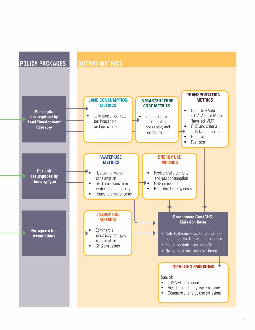
POLICY PACKAGES OUTPUT METRICS

TOTAL GHG EMISSIONS

Sum of:

LDV VMT emissions•

Residential energy use emissions•

Commercial energy use emissions•

ENERGY USE METRICS

Commercial •

electricity and gas

consumption

GHG emissions•

ENERGY USE METRICS

Residential electricity •

and gas consumption

GHG emissions•

Household energy costs•

WATER USE METRICS

Residential water •

consumption

GHG emissions from •

water- related energy

Household water costs•

Greenhouse Gas (GHG)Emission Rates

Auto fuel emissions: Tank-to-wheel •

per gallon; well-to-wheel per gallon

Electricity emissions per kWh•

Natural gas emissions per therm•

TRANSPORTATION METRICS

Light Duty Vehicle •

(LDV) Vehicle Miles

Traveled (VMT)

GHG and criteria •

pollutant emissions

Fuel use•

Fuel cost•

INFRASTRUCTURE COST METRICS

Infrastructure •

cost: total, per

household, and

per capita

LAND CONSUMPTION METRICS

Land consumed: total, •

per household,

and per capita

Per-capita assumptions by

Land Development Category

Per-unitassumptions by Housing Type

Per-square foot assumptions

6

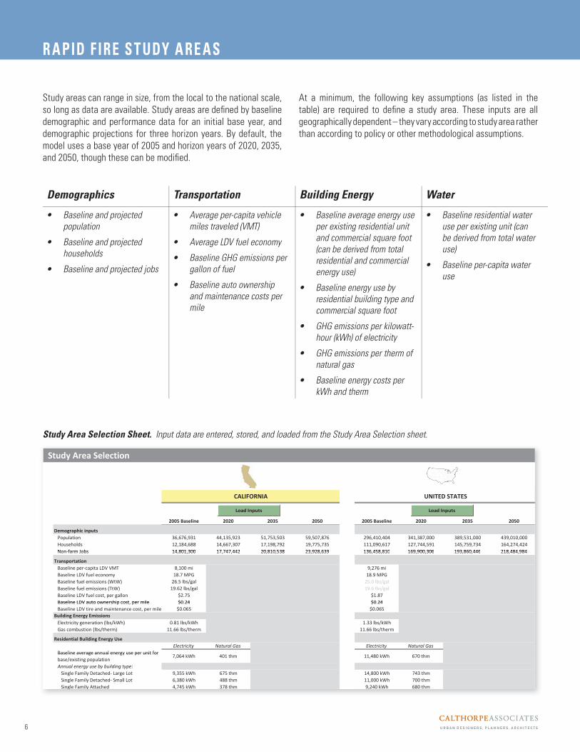
Study areas can range in size, from the local to the national scale,

so long as data are available. Study areas are defi ned by baseline

demographic and performance data for an initial base year, and

demographic projections for three horizon years. By default, the

model uses a base year of 2005 and horizon years of 2020, 2035,

and 2050, though these can be modifi ed.

Study Area Selection

UNITED STATESCALIFORNIA

2005 Baseline 2020 2035 2050 2005 Baseline 2020 2035 2050

Demographic inputsPopulation 36,676,931 44,135,923 51,753,503 59,507,876 296,410,404 341,387,000 389,531,000 439,010,000Households 12,184,688 14,667,307 17,198,792 19,775,735 111,090,617 127,744,591 145,759,734 164,274,424Non farm Jobs 14 801 300 17 747 442 20 810 538 23 928 639 136 458 810 169 900 306 193 860 446 218 484 984

Load InputsLoad Inputs

Non farm Jobs 14,801,300 17,747,442 20,810,538 23,928,639 136,458,810 169,900,306 193,860,446 218,484,984

TransportationBaseline per capita LDV VMT 8,100 mi 9,276 miBaseline LDV fuel economy 18.7 MPG 18.9 MPGBaseline fuel emissions (WtW) 26.5 lbs/gal 25.0 lbs/galBaseline fuel emissions (TtW) 19.62 lbs/gal 19.6 lbs/galBaseline LDV fuel cost, per gallon $2.75 $1.87Baseline LDV auto ownership cost per mile $0 24 $0 24


Baseline LDV auto ownership cost, per mile $0.24 $0.24Baseline LDV tire and maintenance cost, per mile $0.065 $0.065

Building Energy EmissionsElectricity generation (lbs/kWh) 0.81 lbs/kWh 1.33 lbs/kWhGas combustion (lbs/therm) 11.66 lbs/therm 11.66 lbs/therm

Residential Building Energy UseElectricity Natural Gas Electricity Natural Gas

Baseline average annual energy use per unit fork h h k h h


Baseline average annual energy use per unit forbase/existing population

7,064 kWh 401 thm 11,480 kWh 670 thm

Annual energy use by building type:Single Family Detached Large Lot 9,355 kWh 675 thm 14,800 kWh 743 thmSingle Family Detached Small Lot 6,380 kWh 488 thm 11,000 kWh 700 thmSingle Family Attached 4,745 kWh 378 thm 9,240 kWh 680 thm

Load InputsLoad Inputs Load InputsLoad Inputs Load InputsLoad Inputs

Study Area Selection Sheet. Input data are entered, stored, and loaded from the Study Area Selection sheet.

At a minimum, the following key assumptions (as listed in the

table) are required to defi ne a study area. These inputs are all

geographically dependent – they vary according to study area rather

than according to policy or other methodological assumptions.

Demographics Transportation Building Energy Water

Baseline and projected •

population

Baseline and projected •

households

Baseline and projected jobs•

Average per-capita vehicle •

miles traveled (VMT)

Average LDV fuel economy•

Baseline GHG emissions per •

gallon of fuel

Baseline auto ownership •

and maintenance costs per

mile

Baseline average energy use •

per existing residential unit

and commercial square foot

(can be derived from total

residential and commercial

energy use)

Baseline energy use by •

residential building type and

commercial square foot

GHG emissions per kilowatt-•

hour (kWh) of electricity

GHG emissions per therm of •

natural gas

Baseline energy costs per •

kWh and therm

Baseline residential water •

use per existing unit (can

be derived from total water

use)

Baseline per-capita water •

use

R A PID F IRE S T UDY A RE A S

7

The Rapid Fire model analyzes up to four scenarios at a time.

Each scenario consists of two components: a land use option and

a policy package. The land use options vary the patterns of new

growth, while the policy packages vary standards for automobile

technology and fuel composition; building energy and water

effi ciency; and energy generation.

Land Use OptionsThe land use options all accommodate the same amount of

projected population and job growth, but differ in how that

growth is allocated. The user defi nes a land use option by varying

the proportions of growth in each of three Land Development

Categories (LDCs) – Urban, Compact, and Standard. The LDCs

represent distinct forms of land use, ranging from dense, walkable,

mixed-use urban areas that are well served by transit, to lower-

intensity, less walkable places where land uses are segregated

and most trips are made via automobile. Each LDC is associated

with different travel behaviors and a different mix of housing

types and commercial space profi les, as described generally on

the next page.

The Rapid Fire model is loaded with four default land use options –

Business as Usual, Mixed Growth, Smart Growth, and Smart Growth Plus – all which can be modifi ed by the user. The fi gure at

right shows the area of the Scenario Defi nition sheet in which land

use options and the housing unit mixes of each LDC are defi ned.

The defi nition and resulting housing type mix of an example land

use option is outlined in the diagram on page 9.

Land Use Option Section of Scenario Defi nition Sheet. Proportions for land use options and LDCs are set in the Land Use

Option section of the Scenario Defi nition sheet.

L A ND USE OP T IONS

8

Land Use Characteristics Transportation Infrastructure

URBAN Most intense and most mixed LDC, often found within

and directly adjacent to moderate and high density

urban centers. Virtually all ‘Urban’ growth would be

considered infi ll or redevelopment. The majority of

housing in Urban areas is multifamily and attached

single family (townhome). These housing types tend to

consume less water and energy than the larger single

family types found in greater proportion in less urban

locations.

Supported by high levels of regional and local transit

service. Well-connected street networks and the mix and

intensity of uses result in a highly walkable environment

and relatively low dependence on the automobile for

many trips.

Per-capita VMT range: ~ 1,500 to 4,000 per year.

COMPACT Less intense than Urban LDC, but highly walkable with

rich mix of retail, commercial, residential, and civic uses.

The Compact form is most likely to occur as new growth

on the urban edge or large-scale redevelopment. Rich

mix of housing, from multifamily and attached single

family (townhome) to small- and medium-lot single

family homes. Housing types in Compact areas tend to

consume less energy and water than the larger types

found in the Standard LDC.

Well served by regional and local transit service, but may

not benefi t from as much service as Urban growth, and is

less likely to occur around major multimodal hubs. Streets

are well connected and walkable, and destinations such

as schools, shopping, and entertainment areas can

typically be reached via a walk, bike, transit, or short

auto trip.


STANDARD Represents the majority of separate-use auto-oriented

development that has dominated the American suburban

landscape over the past decades. Densities tend to be

lower than Compact LDC, and are generally not highly

mixed or organized to facilitate walking, biking, or transit

service. Can contain a wide variety of housing types,

though medium- and larger-lot single family homes

comprise the majority of this development form; these

larger single family tend to consume more energy and

water than those in the Urban or Compact LDCs.

Not well served by regional transit service (typically),

with most trips made via automobile.


Land Development CategoriesThe Urban, Compact, and Standard LDCs represent distinct forms of

land use. Their general land use characteristics and transportation

infrastructure are described below. These characteristics are all

determined by model inputs that can be entered or adjusted by

the user.

L A ND USE OP T IONS

9

Assumptions by Land Development Category

The housing unit mix assumptions are applied to the housing growth projected for each LDC (determined by the proportion of population growth

allocated to the LDC within a scenario/time period) to produce housing counts by type.

Housing Unit MixThe housing mix assumptions for the three LDCs lead to an overall

mix of housing units for each land use option and time period.

The default housing mix assumptions for the LDCs are intended

to refl ect existing land use patterns and policies, and thus remain

constant for each LDC over time. Housing unit mix assumptions can

be changed to represent shifts in housing demand over time, or to

represent different market conditions among land use options.

Urban areas are comprised of multifamily and attached single

family units. Compact areas contain the widest range of housing

types, from multifamily and attached single family to small-lot

single family units, with a small proportion of large-lot single

family units. Standard development is dominated by large-lot

single family units, with small proportions of other housing types.

The LDC and housing unit mix assumptions for the default “Smart

Growth” land use option are shown below.

Default Housing Mix Assumptions for LDCs

STANDARD LDC

75%

8% 10% 7%

MultifamilyTownhome

Small LotLarge Lot

*

URBAN LDC0%

30%

70%

0%

18%24% 26%

33%

SMART GROWTH LAND USE OPTION

25%20%

*

“Smart Growth”LDC proportion

5%

40%30% 25%

COMPACT LDC

55%

10

2 SELECT POLICY PACKAGE(S)

Click buttons to load policy group options: A B C A BMinimum Moderate High Minimum Moderat

TRANSPORTATION

ICE Vehicle efficiency (mi/gal) 2020 23.7 22.5 24.7 23.7 22.5

2035 27.0 27.1 38.3 27 27.1

2050 27.9 32.7 54.2 27.9 32.7

Fuel price ($/gal, 2005 dollars) 2020 $3.92 $3.92 $3.92 $3.92 $3.92

2035 $5.60 $5.60 $5.60 $5.60 $5.60

2050 $8.00 $8.00 $8.00 $8.00 $8.00

2020 $0.24 $0.54 $0.24 $0.24 $0.54

2035 $0.24 $0.54 $0.24 $0.24 $0.54

2050 $0.24 $0.54 $0.24 $0.24 $0.54

TRANSPORTATION FUEL EMISSION RATES

Well to Wheels Fuel Emissions (lbs CO2e/gal) 2020 24.64 lbs/gal 24.64 lbs/gal 23.84 lbs/gal 24.64 lbs/gal 24.64 lbs/

2035 23.31 lbs/gal 23.31 lbs/gal 21.20 lbs/gal 23.31 lbs/gal 23.31 lbs/


Tank to Wheels Fuel Emissions 2020 17.66 lbs/gal 18.25 lbs/gal 17.66 lbs/gal 17.66 lbs/gal 18.25 lbs/



CO2e EMISSION RATES2020 1 33 lbs/kWh 1 13 lbs/kWh 0 93 lbs/kWh

FULL POLICY GROUPS AUTO and FUEL TE

Residential & commercial building electricity

Auto ownership and maintenance($/mile, 2005 dollars)

A BA B C A BA B C

Rapid Fire policy packages vary standards for automobile technology

and fuel composition, building energy and water effi ciency, and

energy generation. Auto and Fuel Technology assumptions include

those that guide vehicle effi ciency, fuel emissions, and costs;

Building Effi ciency assumptions include building energy and

water use standards as well as utility costs; and Utility Portfolio

assumptions drive the carbon intensity of the power generation

sector.

Policy-based input assumptions are grouped to represent different

levels of improvement in each of these categories. While users can

enter any combination of input assumptions, the policy packages

allow users to instantly activate and switch between sets of

assumptions to compare results. The components of the policy

package categories are outlined in the table below.

As with the land use options, the policy packages can refl ect a

range of futures, from a business-as-usual case that continues

current trends, to a progressive case that represents signifi cant

policy action. Users can enter values to defi ne up to three alternate

policy packages in each category.

Auto and Fuel Technology Building Effi ciency Utility Portfolio

Internal combustion engine (ICE) vehicle •

fuel effi ciency (miles per gallon)

Fuel price ($ per gallon)•

Well-to-wheels GHG emissions from fuel •

(lbs CO2e per gallon)

Tank-to-wheels GHG emissions from fuel •

(lbs CO2e per gallon)

Percent alternative/electric vehicles•

Battery electric vehicle effi ciency •

(miles/kWh)

Plug-in hybrid electric vehicle effi ciency •

(miles/kWh)

New residential energy effi ciency •

(% reduction from 2005 baseline use)

New commercial energy effi ciency •

(% reduction from 2005 baseline use)

New residential water effi ciency •

(% reduction from 2005)

Energy effi ciency/conservation •

improvements for base/existing

residential building stock (year-upon-

year % reduction)

Energy effi ciency/conservation •

improvements for base/existing

commercial space (year-upon-year %

reduction)

Percent of base/existing residential •

buildings replaced each year

Percent of base/existing commercial •

fl oorspace replaced each year

Electricity price ($ per kWh)•

Natural gas price ($ per kWh)•

Water price ($ per acre foot)•

Residential & commercial building •

electricity emissions (lbs CO2e per kWh)

Residential & commercial building •

natural gas emissions (lbs CO2e per

therm)

*

Policy Package Selection Section of Scenario Defi nition Sheet. The policy packages are organized in sections on the ‘Scenario

Defi nition’ sheet as shown below. Clicking on the buttons labeled A,

B, and C at the top of each column loads input values to the ‘Active

Scenario’ column located at the right of the ‘Utility Portfolio’ section (not

shown). Users can select a ’Full Policy Group’ of minimum, moderate,

or high options, or they can select an option for each individual policy

group. Once selected, the cells containing the active input values are

highlighted in yellow (* ). In this sample view, the ‘moderate’ level full

policy group is selected.

P OL ICY PAC K AGE A S SUMP T IONS

11

TRANSPORTATION METRICS

Light Duty Vehicle (LDV) •

Vehicle Miles Traveled

(VMT)

Fuel Consumed (gal)•

Fuel Cost ($)•

Transportation •

Electricity Consumed

(kWh)

Transportation •

Electricity Cost ($)

Transportation •

Electricity CO2e

Emissions (MMT)

ICE Fuel Combustion •

CO2e Emissions (MMT)

ICE Full Fuel Lifecycle •

CO2e Emissions (MMT)

Criteria Pollutant •

Emissions (tons)

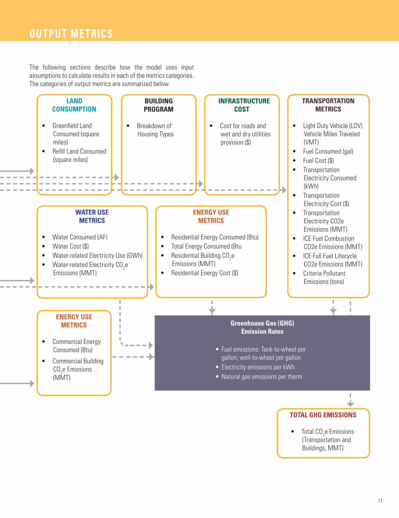
The following sections describe how the model uses input

assumptions to calculate results in each of the metrics categories.

The categories of output metrics are summarized below.

OU T PU T ME T RIC S

TOTAL GHG EMISSIONS

Total CO• 2e Emissions

(Transportation and

Buildings, MMT)

ENERGY USE METRICS

Commercial Energy •

Consumed (Btu)

Commercial Building •

CO2e Emissions

(MMT)

ENERGY USE METRICS

Residential Energy Consumed (Btu)•

Total Energy Consumed (Btu•

Residential Building CO• 2e

Emissions (MMT)

Residential Energy Cost ($)•

WATER USE METRICS

Water Consumed (AF)•

Water Cost ($)•

Water-related Electricity Use (GWh)•

Water-related Electricity CO• 2e

Emissions (MMT)

Greenhouse Gas (GHG)Emission Rates

Fuel emissions: Tank-to-wheel per •

gallon; well-to-wheel per gallon

Electricity emissions per kWh•

Natural gas emissions per therm•

INFRASTRUCTURE COST

Cost for roads and •

wet and dry utilities

provision ($)

BUILDINGPROGRAM

Breakdown of •

Housing Types

LANDCONSUMPTION

Greenfi eld Land •

Consumed (square

miles)

Refi ll Land Consumed •

(square miles)

12

Land consumption includes all land that will be developed to

accommodate population and job growth, including residential and

employment areas, transportation alignments, open space, and

public lands. The Rapid Fire model estimates land consumption

using per-capita rates of land consumption, which vary by Land

Development Category and the distribution of growth into

greenfi eld or refi ll development. Default rates are based on studies

of existing and planned development, and can be adjusted by the

user.

Land consumption includes both refi ll and greenfi eld growth.

Refi ll growth includes all development that may occur within

the bounds of already-developed, urbanized areas, including

infi ll, redevelopment, and greyfi eld and brownfi eld development.

Greenfi eld growth refers to development that occurs on land

that has not previously been developed or otherwise impacted,

including agricultural land, forest land, desert land and other

virgin sites. Only greenfi eld growth is counted towards the “new

land consumption” of a scenario. The default land consumption

characteristics for the three LDCs are as follows:

Urban: Comprised entirely of infi ll, redevelopment, greyfi eld,

and brownfi eld growth, the Urban LDC consumes no greenfi eld

acreage per capita.

Compact: Representing a combination of smart mixed-use

growth in and around the urban edge (greenfi eld growth) as well as

larger-scale greyfi eld growth within urban areas, the Compact LDC

consumes a moderate acreage per capita. The land consumption

rate for Compact growth is determined in part by the proportion of

growth allocated to refi ll versus greenfi eld sites.

ACRES REFILL GROWTH

ACRES GREENFIELD GROWTH

(NEW LAND CONSUMPTION)

Refi llacres

per capita

Greenfi eld acres

per capita

Population growth byLand Development Cateorgy and Growth Type (Refi ll or Greenfi eld)

Standard: Generally consisting of lower-density, auto-oriented

residential and commercial development, the Standard LDC

consumes the highest acreage per capita since most, if not all,

growth occurs on greenfi eld land. The new land consumption

of a scenario is largely dictated by its proportion of Standard

development.

The specifi c allocation of growth to either refi ll or greenfi eld land

in each LDC and time period can vary by land use option. By setting

assumptions for the proportion of refi ll growth and greenfi eld land

consumption, as well as the intensity of greenfi eld growth in terms

of acres consumed per capita, users can model a range of land-use

policy options, from business-as-usual growth, to the application

of urban growth boundaries, to a restriction of growth to refi ll

parcels and sites only.

A land development profi le resulting from the LDC mix of the Rapid

Fire default “Smart Growth” land use option is illustrated in the

fi gure below.

URBANUrban Refi ll

COMPACTCompact Refi ll

Compact Greenfi eld

STANDARDStandard Greenfi eld

Refi ll Growth and Greenfi eld Land Consumption

The LDCs differ signifi cantly in the population

allocated to either refi ll growth or greenfi eld

land. The assumed proportions for Urban

and Standard are straightforward: all Urban

development takes place as refi ll growth,

while virtually all Standard development takes

place on greenfi eld land. These characteristics

are elemental to the Urban and Standard LDC

defi nitions. The land consumption characteristics

of Compact development, however, can vary

signifi cantly over time, by scenario, and

by geographic area. The incremental land

consumption rate of the Compact LDC is largely

dependent on the assumed proportion of refi ll

growth vs. development on new land.

Land Development Profi le of “Smart Growth” Land Use Option (Illustrative Only)

L A ND CONSUMP T ION

URBANURBAN35%35%

STANDARDSTANDARD10%10%

40% Greenfi eld

40% Greenfi eld6060

8080100100

20204040

00

COMPACTCOMPACT55%55%

100% Greenfi eld (0% Refi ll)

100%

Refi

ll (0

% G

reen

fi eld)

13

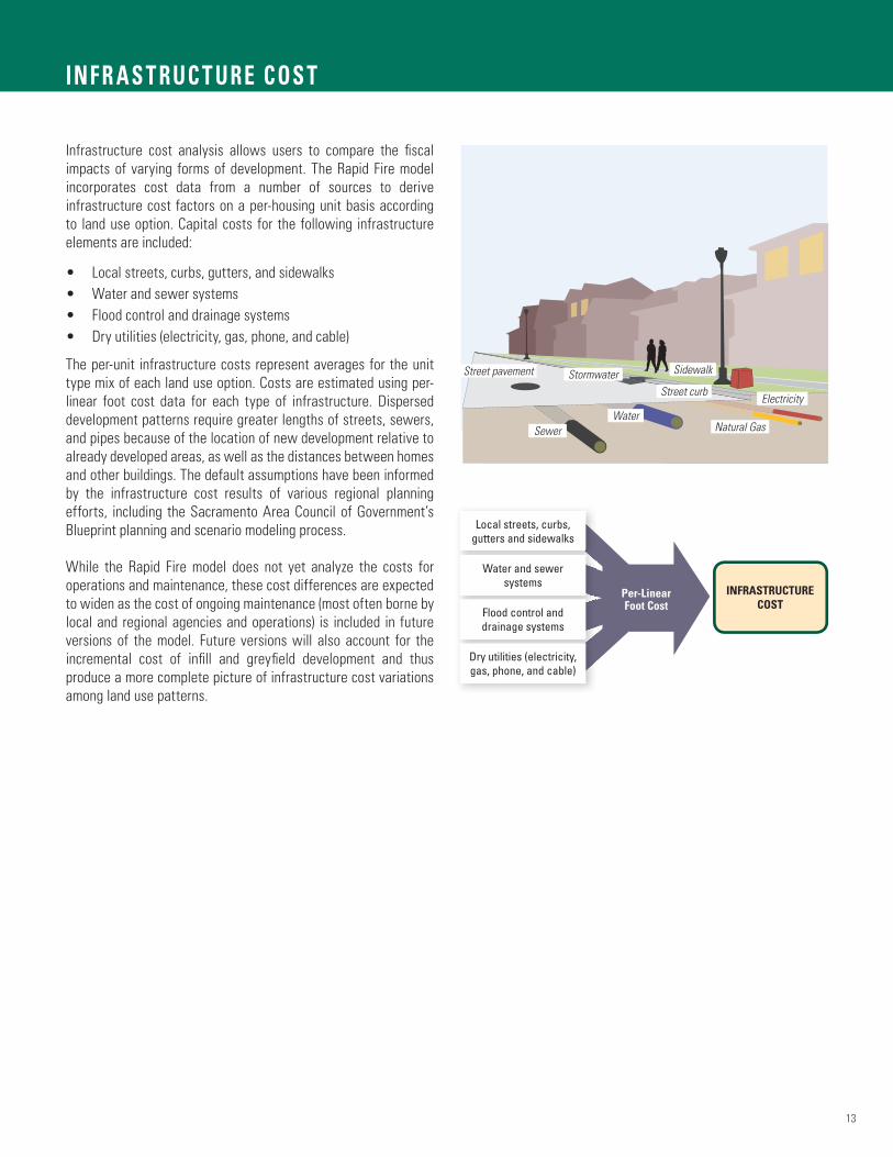
Infrastructure cost analysis allows users to compare the fi scal

impacts of varying forms of development. The Rapid Fire model

incorporates cost data from a number of sources to derive

infrastructure cost factors on a per-housing unit basis according

to land use option. Capital costs for the following infrastructure

elements are included:

Local streets, curbs, gutters, and sidewalks•

Water and sewer systems•

Flood control and drainage systems•

Dry utilities (electricity, gas, phone, and cable)•

The per-unit infrastructure costs represent averages for the unit

type mix of each land use option. Costs are estimated using per-

linear foot cost data for each type of infrastructure. Dispersed

development patterns require greater lengths of streets, sewers,

and pipes because of the location of new development relative to

already developed areas, as well as the distances between homes

and other buildings. The default assumptions have been informed

by the infrastructure cost results of various regional planning

efforts, including the Sacramento Area Council of Government’s

Blueprint planning and scenario modeling process.

While the Rapid Fire model does not yet analyze the costs for

operations and maintenance, these cost differences are expected

to widen as the cost of ongoing maintenance (most often borne by

local and regional agencies and operations) is included in future

versions of the model. Future versions will also account for the

incremental cost of infi ll and greyfi eld development and thus

produce a more complete picture of infrastructure cost variations

among land use patterns.

INFRASTRUCTURE COST

Local streets, curbs, gutters and sidewalks

Water and sewer systems

Flood control and drainage systems

Dry utilities (electricity, gas, phone, and cable)

Per-LinearFoot Cost

INF R A S T RUC T URE COS T

Street curb

Street pavement

Natural GasSewer

Water

Sidewalk

Electricity

Stormwater

Street curb

Street pavement

Natural GasSewer

Water

Sidewalk

Electricity

Stormwater

14

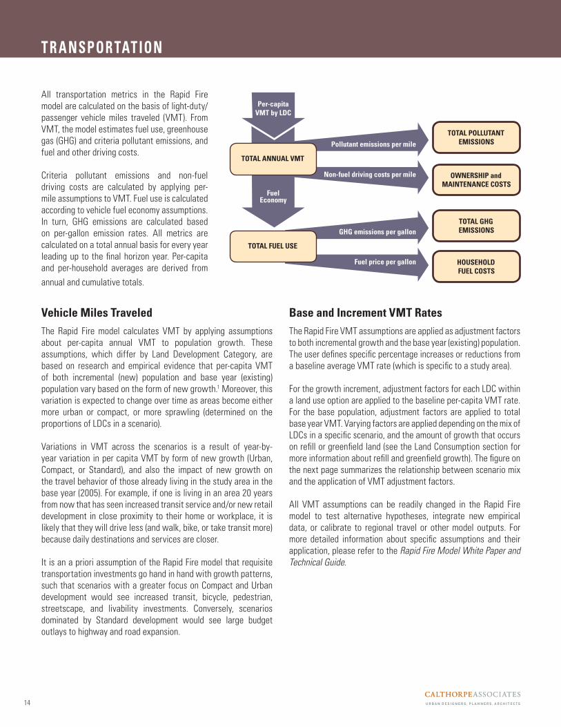
All transportation metrics in the Rapid Fire

model are calculated on the basis of light-duty/

passenger vehicle miles traveled (VMT). From

VMT, the model estimates fuel use, greenhouse

gas (GHG) and criteria pollutant emissions, and

fuel and other driving costs.

Criteria pollutant emissions and non-fuel

driving costs are calculated by applying per-

mile assumptions to VMT. Fuel use is calculated

according to vehicle fuel economy assumptions.

In turn, GHG emissions are calculated based

on per-gallon emission rates. All metrics are

calculated on a total annual basis for every year

leading up to the fi nal horizon year. Per-capita

and per-household averages are derived from

annual and cumulative totals.

T R A NSP OR TAT IONVehicle Miles Traveled

TOTAL FUEL USE

Non-fuel driving costs per mile OWNERSHIP andMAINTENANCE COSTS

Pollutant emissions per mileTOTAL POLLUTANT

EMISSIONS

Fuel price per gallon HOUSEHOLDFUEL COSTS

GHG emissions per gallonTOTAL GHGEMISSIONS

FuelEconomy

TOTAL ANNUAL VMT

Per-capitaVMT by LDC

Vehicle Miles TraveledThe Rapid Fire model calculates VMT by applying assumptions

about per-capita annual VMT to population growth. These

assumptions, which differ by Land Development Category, are

based on research and empirical evidence that per-capita VMT

of both incremental (new) population and base year (existing)

population vary based on the form of new growth.1 Moreover, this

variation is expected to change over time as areas become either

more urban or compact, or more sprawling (determined on the

proportions of LDCs in a scenario).

Variations in VMT across the scenarios is a result of year-by-

year variation in per capita VMT by form of new growth (Urban,

Compact, or Standard), and also the impact of new growth on

the travel behavior of those already living in the study area in the

base year (2005). For example, if one is living in an area 20 years

from now that has seen increased transit service and/or new retail

development in close proximity to their home or workplace, it is

likely that they will drive less (and walk, bike, or take transit more)

because daily destinations and services are closer.

It is an a priori assumption of the Rapid Fire model that requisite

transportation investments go hand in hand with growth patterns,

such that scenarios with a greater focus on Compact and Urban

development would see increased transit, bicycle, pedestrian,

streetscape, and livability investments. Conversely, scenarios

dominated by Standard development would see large budget

outlays to highway and road expansion.

Base and Increment VMT RatesThe Rapid Fire VMT assumptions are applied as adjustment factors

to both incremental growth and the base year (existing) population.

The user defi nes specifi c percentage increases or reductions from

a baseline average VMT rate (which is specifi c to a study area).

For the growth increment, adjustment factors for each LDC within

a land use option are applied to the baseline per-capita VMT rate.

For the base population, adjustment factors are applied to total

base year VMT. Varying factors are applied depending on the mix of

LDCs in a specifi c scenario, and the amount of growth that occurs

on refi ll or greenfi eld land (see the Land Consumption section for

more information about refi ll and greenfi eld growth). The fi gure on

the next page summarizes the relationship between scenario mix

and the application of VMT adjustment factors.

All VMT assumptions can be readily changed in the Rapid Fire

model to test alternative hypotheses, integrate new empirical

data, or calibrate to regional travel or other model outputs. For

more detailed information about specifi c assumptions and their

application, please refer to the Rapid Fire Model White Paper and

Technical Guide.

15

development exceeds 55%

Escalation+

Deceleration–

+

+

UrbanCompactStandard

ReductionReductionEscalation


ReductionReductionEscalation


ReductionReductionNo change

No change

Standard development exceeds 55%BUSINESS as USUAL

MIXED GROWTH

SMART GROWTH

SCENARIO TYPE LDC PROPORTION

SCENARIO CLASSIFICATION

BASE

VMT ADJUSTMENTS

INCREMENT

VMT ADJUSTMENTS

Scenario Tipping Point Range:

45 - 55%

Detailed VMT Assumptions Sheet. Inputs are entered, stored, and loaded from the Study Area Selection sheet.

Detailed VMT Assumptions

Baseline per capita LDV VMT1990 7,377

Load VMT Assumptions Restore Defaults2005 9,276 mi

BASE VMT ADJUSTMENT ASSUMPTIONSVMT Escalation/Deceleration Rates for the Base (Existing Environment)

ESCALATION RATE: Standard Impact on Base VMT in Trend Scenario

Load VMT Assumptions Restore Defaults

2005 2020 0.50% Annual Rate2020 2035 0.00% Annual Rate2035 2050 0.00% Annual Rate

ESCALATION RATE: Standard Impact on Base VMT in Trend Scenario

DECELERATION RATE: Compact+Urban Growth Impact on Base VMT in Smart Scenarios


2005 2020 0.50% Maximum Annual Rate2020 2035 0.563% Maximum Annual Rate2035 2050 0.63% Maximum Annual Rate

Intermediate Range Definition:

These percentages are used to determine when to apply escalation/deceleration rates, as well as the appropriate VMT by LDC.


Standard Low: 45% or less of scenario is Standard GrowthStandard High: 55% or more of scenario is Standard Growth

INCREMENT VMT ASSUMPTIONS

These percentages are used to determine when to apply escalation/deceleration rates, as well as the appropriate VMT by LDC.


INCREMENT VMT ASSUMPTIONSAdjustment factors relative to baseline average VMT (Applied to incremental population only)

Standard Standard Adjustment Factor for Trend Scenarios 20% 11,131 50% 13,914 20% 11,131 60% 14,842 35% 12,523 60% 14,842 55% 14,37Standard Adjustment Factor for Conservative Scenarios 20% 11,131 50% 13,914 15% 10,667 40% 12,986 15% 10,667 40% 12,986 15% 10,66

2035 Adjustment Rate

for Refill for Greenfield for Refill

2020 Adjustment Rate

for Refill for Greenfield

2006 Starting Point Adjustment Rate

for Refill for Greenfield


Standard Adjustment Factor for Conservative Scenarios 20% 11,131 50% 13,914 15% 10,667 40% 12,986 15% 10,667 40% 12,986 15% 10,66Standard VMT per Capita in Smart Growth Scenarios 20% 11,131 50% 13,914 10% 10,204 25% 11,595 10% 10,204 20% 11,131 10% 10,20

Standard VMT per Capita in Ultra Smart Growth Scenarios 20% 11,131 50% 13,914 10% 10,204 25% 11,595 10% 10,204 20% 11,131 10% 10,20Compact Compact Adjustment Factor for Trend Scenarios 20% 7,421 10% 8,348 20% 7,421 10% 8,348 20% 7,421 10% 8,348 20% 7,42

Compact Adjustment Factor for Conservative Scenarios 20% 7,421 10% 8,348 25% 6,957 15% 7,885 30% 6,493 20% 7,421 35% 6,029Standard VMT per Capita in Smart Growth Scenarios 20% 7,421 10% 8,348 35% 6,029 20% 7,421 40% 5,566 25% 6,957 45% 5,102


Standard VMT per Capita in Ultra Smart Growth Scenarios 20% 7,421 10% 8,348 35% 6,029 20% 7,421 40% 5,566 25% 6,957 45% 5,102Urban Urban Adjustment Factor for Trend Scenarios 40% 5,566 35% 6,029 40% 5,566 35% 6,029 40% 5,566 35% 6,029 40% 5,566

Urban Adjustment Factor for Conservative Scenarios 40% 5,566 35% 6,029 45% 5,102 40% 5,566 50% 4,638 45% 5,102 55% 4,174Standard VMT per Capita in Smart Growth Scenarios 40% 5,566 35% 6,029 50% 4,638 45% 5,102 60% 3,710 50% 4,638 70% 2,783

Standard VMT per Capita in Ultra Smart Growth Scenarios 40% 5,566 35% 6,029 50% 4,638 45% 5,102 60% 3,710 50% 4,638 70% 2,783


Resulting VMT per Capita, by Land Development Category and Scenario

VMT% Change from

2005VMT

% Change from2005

VMT% Change from

2005VMT

% Change from2005

2006 Starting Values 2020 2035 2050


2005 2005 2005 2005Standard Standard VMT per Capita in Trend Scenario 13,914 50% 14,842 60% 14,842 60% 14,842 60%

Standard VMT per Capita in Conservative Scenario 13,914 50% 12,986 40% 12,986 40% 12,986 40%Standard VMT per Capita in Smart Growth Scenario 13,914 50% 11,595 25% 11,131 20% 10,667 15%

Standard VMT per Capita in Ultra Smart Growth Scenario 13,914 50% 11,595 25% 11,131 20% 10,667 15%Compact Compact VMT per Capita in Trend Scenario 8,209 12% 8,209 12% 8,209 12% 8,209 12%


Compact VMT per Capita in Conservative Scenario 8,163 12% 7,699 17% 7,143 23% 6,586 29%Compact VMT per Capita in Smart Growth Scenario 7,977 14% 6,864 26% 6,261 33% 5,658 39%

Compact VMT per Capita in Ultra Smart Growth Scenario 7,699 17% 6,447 31% 5,844 37% 5,380 42%Urban Urban VMT per Capita in Trend Scenario 5,566 40% 5,566 40% 5,566 40% 5,566 40%

Urban VMT per Capita in Conservative Scenario 5,566 40% 5,102 45% 4,638 50% 4,174 55%Urban VMT per Capita in Smart Growth Scenario 5 566 40% 4 638 50% 3 710 60% 2 783 70%


Urban VMT per Capita in Smart Growth Scenario 5,566 40% 4,638 50% 3,710 60% 2,783 70%Urban VMT per Capita in Ultra Smart Growth Scenario 5 566 40% 4 638 50% 3 710 60% 2 783 70%


T R A NSP OR TAT IONVehicle Miles Traveled

Base and Increment VMT Adjustment Factors by Scenario Type. If a scenario is more oriented towards Standard development, then

VMT is calculated to increase at a greater rate than if a scenario is

more focused towards Urban and Compact growth. Overall scenario

orientation is determined using a “tipping point” range. If Standard

development falls below the range, adjustment factors refl ective of

progressively decreasing VMT are applied; conversely, if Standard

development surpasses the range, factors refl ective of increasing

VMT are applied. If Standard development falls within the tipping

point range, then driving behavior does not change further beyond the

default rates.

16

The Rapid Fire model calculates transportation fuel use, GHG and

criteria pollutant emissions, and costs by applying policy-based

assumptions to output VMT. Each metric is calculated on a total

annual basis for all years in the model.

Fuel UseLDV fuel consumption is determined by applying on-road average

fuel economy assumptions (miles per gallon of gasoline equivalent2,

or MPG) to VMT in each year for each scenario. Fuel economy

changes year upon year according to horizon-year projections.

Policy-based projections signifi cantly affect fuel consumption,

and thus GHG emission and fuel cost results. Users can easily

input and test alternate assumptions, such as compliance with

California’s Pavley Clean Car Standards or the federal CAFE

standard, either in isolation or in combination with fuel carbon

intensity assumptions.

Electric and other low-emission vehicles will play an important role

in reducing GHG emissions. The Rapid Fire model can refl ect their

impacts in either of two ways: through the use of fuel economy and

emission assumptions that implicitly capture the effects of their

inclusion in the fl eet3, or through the use of separate assumptions

for electric and conventional (internal combustion engine) vehicles.

More information about how the model estimates electric and

alternative vehicle impacts can be found in the Rapid Fire Model

White Paper and Technical Guide.

GHG EmissionsTransportation GHG emissions are calculated by applying carbon

intensity assumptions, expressed in pounds of carbon dioxide

equivalent (CO2e) per gallon, to fuel consumption. Carbon intensity

changes year upon year according to horizon-year projections.

Projections can represent a range of standards, from a trend

future in which carbon intensity remains constant or sees limited

improvement, to a more aggressive policy-based future in which

the carbon intensity of fuel declines signifi cantly as low-carbon

fuels, such as cellulosic ethanol and renewable biodiesel, comprise

a higher proportion of fuel use.

The Rapid Fire model was designed to calculate emissions that

occur upon fuel combustion (“tank-to-wheel” emissions), as well

as those emitted during the full fuel lifecycle, from extraction and

processing to transport and storage (“well-to-wheel” emissions).

Users can look to either or both; typically, emission inventories

compare tank-to-wheel emissions, although full well-to-wheel

assessments are critical to developing climate change mitigation

strategies. The Rapid Fire model is able to calculate both types

of emission rates based on fuel mix assumptions, enabling an

analysis of the role of fuel carbon intensity standards in meeting

GHG reduction goals. More often, though, users will opt to model

tank-to-wheel emissions on the basis of a baseline carbon intensity

factor and projected reductions from it to each horizon year.

Fuel and other Driving CostsThe Rapid Fire model estimates three components of transportation

costs, including fuel, auto ownership, and tires and maintenance.

These costs are calculated separately using different assumptions.

Fuel costs are calculated by multiplying fuel consumed by fuel

price per gallon. Auto ownership and tire and maintenance costs

are each calculated by multiplying VMT by an average price-per-

mile factor. All per-gallon and per-mile prices change year upon

year according to horizon-year projections.

Pricing Effects

Because fuel price, along with other driving costs, have been

shown to have both short- and long-term effects on driving

decisions, the Rapid Fire model allows users the option to “turn

on” sensitivity to changes in per-mile driving costs to estimate

changes in VMT due to pricing. Research into historic patterns has

quantifi ed relationships among the interrelated factors of VMT

and automobile fuel economy with costs including fuel price and

taxes; automobile ownership, insurance, and maintenance costs;

and parking, toll, and congestion charges. The results, expressed

as an “elasticity” of change in one factor with respect to change in

another, can be used to estimate the effects of specifi c policy- or

program-based assumptions on VMT.

T R A NSP OR TAT IONFuel Use, Emissions, and Costs

17

Baseline Residential Energy Use. Because larger homes require

more energy to heat and cool, home size is generally correlated with

a household’s overall energy consumption. Scenarios with a greater

proportion of the Standard Land Development Category, which include

primarily single-family detached homes, will require more energy –

and produce more GHG emissions – than scenarios with a greater

proportion of Compact or Urban areas, which include more attached

and multifamily homes. Energy use also varies by climate zone, which

can be refl ected in the Rapid Fire model.

Baseline Annual Household Energy Use by Building Type*

Large Lot Single Family

Small Lot Single Family

Attached Single Family

Multifamily

100 million Btu 71 million Btu 54 million Btu 38 million Btu

* California averages, including residential electricity and natural

gas use. Derived from the California Energy Commission Statewide

Residential Appliance Saturation Survey (RASS), 2004.

The Rapid Fire model calculates residential and commercial

building energy use for both new and existing buildings. Scenarios

vary in their building energy use profi les due to their building

program and policy-based assumptions about improvements in

energy effi ciency.

Residential Energy ConsumptionResidential energy use in the Rapid Fire model is calculated as a

function of three basic sets of assumptions: a) average base-year

energy use for existing units; b) base-year (2005) energy use for

new units by building type; and c) reductions in building energy

use resulting from advances in building energy effi ciency policy

and technology.

Energy Use of Base/Existing Buildings

Average per-household energy use for existing units is derived

from total residential sector electricity and gas use and number

of housing units in the baseline year (2005). The energy used by

the population of existing units is expected to decline over time, as

buildings are replaced, retrofi tted, or upgraded. The extent of future

energy savings due to each of these conditions are determined by

user-specifi ed rates.

Energy Use of New Buildings

Energy use for new units is calculated using per-unit factors for

annual electricity and gas use. Reductions are applied to the

baseline factors to refl ect the assumption that, year-upon-year,

new construction will be built to meet higher effi ciency standards.

It is also expected that new buildings can see further improvement

over the time span of the model (for instance, a building built in

2011 may be retrofi t by 2035 to meet even higher standards).

The application of the energy use reduction assumptions applied

to both new and existing units is shown in the fl ow chart on the

following page.

Commercial Energy Consumption As for residential energy use, commercial energy use in the

Rapid Fire model is calculated as a function of three basic sets of

assumptions: a) per-employee fl oorspace factors, b) baseline (2005)

energy intensity factors, and c) reductions in building energy use

resulting from advances in building energy effi ciency policy and

technology.

Energy Use of Base/Existing Buildings

Average per-square foot energy use for existing commercial

buildings is derived from total commercial sector electricity and

gas use and a fl oorspace estimate for the baseline year (2005).

The energy used by existing buildings is expected to decline over

time, as buildings are replaced, retrofi tted, or upgraded. The

extent of future energy savings due to each of these conditions

are determined by user-specifi ed rates.

Energy Use of New Buildings

Energy use for new commercial fl oorspace is calculated using per-

square foot energy intensity factors for annual electricity and gas

use. Reductions are applied to the baseline factors to refl ect the

assumption that, year-upon-year, new construction will be built

to meet higher effi ciency standards. It is also expected that new

buildings can see further improvement over the time span of the

model (for instance, a building built in 2011 may be retrofi t by 2035

to meet even higher standards). The application of the energy use

reduction assumptions applied to both new and existing units is

shown in the fl ow chart on the following page.

The amount of new commercial space in each scenario is calculated

using assumptions about the number of employees by commercial

space type (offi ce, retail, or warehouse), and the amount of

fl oorspace required per employee in each of the three Land

Development Categories. Floorspace requirements are highest

in the Standard LDC, and lowest in the Urban LDC. The number

of employees by type, which is held constant for all scenarios, is

projected based on demographic assumption inputs.

RE SIDEN T I A L and COMMERCI A L BUIL DING ENERGYEnergy Consumption

18

Total Buildings

Replacement Rate

Non-Replaced Buildings Replacement Buildings

Base / Existing Buildings

(Residential Units or Commercial Floorspace)

Growth Increment Buildings

(Residential Units by Type or Commercial Floorspace)

Energy Use Reduction Factors

Upgrade Effi ciency Factor ‘A’

Effi ciency improvements

and conservation

measures

New Effi ciency Factor ‘B’

New construction

standards

New Effi ciency Factor ‘D’

New construction

standards

Upgrade Effi ciency Factor ‘C’

Ongoing effi ciency

improvements and

conservation measures

Upgrade Effi ciency Factor ‘E’

Ongoing effi ciency

improvements nad

conservation measures

ANNUAL ENERGY USE OF TOTAL BUILDINGS

ENERGY USE OF NEW/INCREMENT

BUILDINGSENERGY USE OF BASE / EXISTING BUILDINGS

RE SIDEN T I A L and COMMERCI A L BUIL DING ENERGYEnergy Consumption

19

Resource Mix and Emission Rates. Electricity greenhouse gas (CO2e) emissions vary based on the mix of resources used. As the share

of clean and renewable energy sources in the electricity generation portfolio is increased, the average electricity emission rate will decrease.

Electricity emissions are estimated based on assumed rates in 2020, 2035, and 2050. The diagram below illustrates a hypothetical move toward a

cleaner portfolio and lower emission rate.

Greenhouse Gas Emissions Building GHG emissions include total emissions from residential

and commercial electricity and natural gas use. Emission results

are calculated based on energy consumption and emission rates,

which are assumed to vary according to the mix of resources used

to generate energy. The baseline and projected emission rates are

measured per unit of energy consumed (kilowatt-hour or therm),

and include carbon dioxide, methane, and nitrous oxide emissions

in units of carbon dioxide equivalent (CO2e). The same emission

rates are applied to the energy used by residential and commercial

buildings.

Emission Rate Assumptions

Projections are made for the horizon years of 2020, 2035, and

2050, with rates following a straight-line trend in between.

The emission rate for electricity generation can be expected to

decline over time, while that for natural gas use can be expected

to remain constant. As with all Rapid Fire assumptions, users

can enter different inputs to test the results of different policy-

based projections, for instance comparing the effects of achieving

California’s 33% Renewables Portfolio Standard (RPS) by 2020, or

by a later date.

When available, absolute projections based on analyses specifi c

to a state or region should be used. Because emissions from

electricity are subject to a number of interrelated variables that can

affect resource mix and emission rates into the future – including

fuel price and availability, generation costs, energy use effi ciency,

the market penetration of renewable energy technologies, and

the amount of electricity imported from other areas – rates

are technically challenging to estimate. In the absence of such

projections, users can enter emission rate projections calculated

as simple percentage reductions from the baseline emission rate.

For a detailed discussion of energy emission rate assumptions and

their application in the model, please refer to the Rapid Fire Model

White Paper and Technical Guide.

Energy CostsResidential and commercial energy costs are calculated on the

basis of energy use and price assumptions. The model applies

separate retail price factors to residential and commercial

electricity and natural gas use. Price projection assumptions are

expressed in constant dollars, and like all assumptions are entered

for the horizon years of 2020, 2035, and 2050. Between horizon

years, prices are assumed to follow a straight-line trend.

Electricity prices are expected to increase over time, in response

to changes in the portfolio mix and other factors such as the cost

of electricity generation resources, various infrastructure costs,

overall supply and demand, and potential regulations. Electricity

price projections can be estimated to correspond generally with

the portfolio mix inherent to the chosen GHG emission rate

assumptions, or estimated as simple percentage increases over

the baseline price. Natural gas price projections can be estimated

similarly.

RE SIDEN T I A L and COMMERCI A L BUIL DING ENERGYGHG Emissions and Costs

Renewables 20%

Hydro 20%

Natural Gas 34%

Nuclear 12%

Coal 15%

Renewables 64%

Hydroelectric 15%

Natural Gas 5%

Nuclear 12%

Coal 5%

Biom

ass

Geoth

erm

al

Small

Hyd

ro

Solar P

hoto

volta

ics

Solar T

herm

al

Win

dBio

gas

Biom

ass

Bioga

s

Geoth

erm

al

Small

Hyd

ro

Solar P

hoto

volta

ics

Solar T

herm

al

Win

d

2020~600 lbs CO2e/MWh

2050~300 lbs CO2e/MWh

20

Water ConsumptionResidential water use in the Rapid Fire model is calculated as a

function of three basic sets of assumptions: a) average base-year

water use for existing units; b) base-year (2005) water use for

new units by building type; and c) reductions in building water use

resulting from advances in water effi ciency policy and technology.

Water Use of Base/Existing Buildings

Average per-household water use for existing units is derived

from total residential sector water use and housing units for the

baseline year (2005). The energy used by the population of existing

units is expected to decline over time, as water-saving measures

are implemented. The extent of future energy savings due to

each of these conditions are determined by user-specifi ed rates –

expressed as percentage reductions from baseline use – to each

horizon year.

Water Use of New Buildings

Water use for new units is calculated using annual per-unit usage

factors, which vary by building type. Reductions are applied to

the baseline factors to refl ect the assumption that, year-upon-

year, new homes will be built with the technology to meet higher

effi ciency standards. It is also expected that new buildings can

see further improvement over the time span of the model (for

instance, a building built in 2011 may be upgraded by 2035 to meet

even higher standards). The application of the water use reduction

assumptions applied to both new and existing units is represented

in the fl ow chart below.

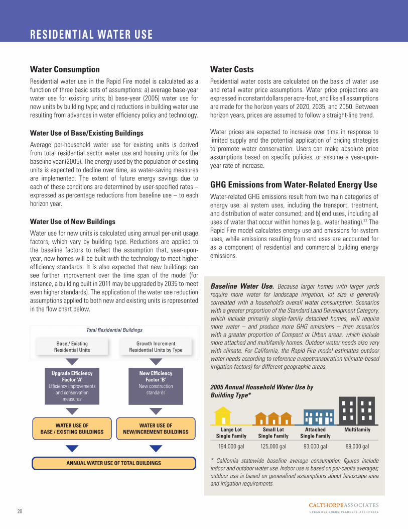
Baseline Water Use. Because larger homes with larger yards

require more water for landscape irrigation, lot size is generally

correlated with a household’s overall water consumption. Scenarios

with a greater proportion of the Standard Land Development Category,

which include primarily single-family detached homes, will require

more water – and produce more GHG emissions – than scenarios

with a greater proportion of Compact or Urban areas, which include

more attached and multifamily homes. Outdoor water needs also vary

with climate. For California, the Rapid Fire model estimates outdoor

water needs according to reference evapotranspiration (climate-based

irrigation factors) for different geographic areas.

Large Lot Single Family

Small Lot Single Family

Attached Single Family

Multifamily

194,000 gal 125,000 gal 93,000 gal 89,000 gal

* California statewide baseline average consumption fi gures include

indoor and outdoor water use. Indoor use is based on per-capita averages;

outdoor use is based on generalized assumptions about landscape area

and irrigation requirements.

ANNUAL WATER USE OF TOTAL BUILDINGS

Total Residential Buildings

Base / ExistingResidential Units

Growth IncrementResidential Units by Type

WATER USE OF BASE / EXISTING BUILDINGS

WATER USE OF NEW/INCREMENT BUILDINGS

Upgrade Effi ciency Factor ‘A’

Effi ciency improvements

and conservation

measures

New Effi ciency Factor ‘B’

New construction

standards

Water CostsResidential water costs are calculated on the basis of water use

and retail water price assumptions. Water price projections are

expressed in constant dollars per acre-foot, and like all assumptions

are made for the horizon years of 2020, 2035, and 2050. Between

horizon years, prices are assumed to follow a straight-line trend.

Water prices are expected to increase over time in response to

limited supply and the potential application of pricing strategies

to promote water conservation. Users can make absolute price

assumptions based on specifi c policies, or assume a year-upon-

year rate of increase.

GHG Emissions from Water-Related Energy UseWater-related GHG emissions result from two main categories of

energy use: a) system uses, including the transport, treatment,

and distribution of water consumed; and b) end uses, including all

uses of water that occur within homes (e.g., water heating).22 The

Rapid Fire model calculates energy use and emissions for system

uses, while emissions resulting from end uses are accounted for

as a component of residential and commercial building energy

emissions.

RE SIDEN T I A L WAT ER USEWater Consumptions, Costs, and GHG Emissions

2005 Annual Household Water Use by Building Type*

21

Viewing Model ResultsUsers can view model outputs through the model’s static results

summary (the “Results” sheet) or the automated interface of

the “Interactive Results” sheet. The automated interface allows

users to customize the results display according to the following

parameters:

Horizon year (2020, 2035, or 2050)•

Annual (single-year) or cumulative (multiple-year leading up to •

horizon year) metrics

Total, per capita, or per household basis for metrics•

Comparison of annual metrics against historic baseline year •

(1990 or 2005)

Below is a sample view of the “Interactive Results” sheet.

MODEL RE SULT S

Interactive Results Sheet. Results are automatically displayed according to the parameters selected.

RESULTS (Interactive)Study Area: United States

1 Select a horizon year for which to show results: 2050 Demographics 1990 2005 2020 2035 2050

Population 248,709,873 296,410,404 341,387,000 389,531,000 439,010,000

2 Select ANNUAL or CUMULATIVE results: ANNUAL Households 91,947,410 111,090,617 127,744,591 145,759,734 164,274,424

3 Select total, per capita, or per household results: per Household

4 Select a historical baseline year against which tocompare selected horizon year results:

2005

5 Click to see results:

6 If needed, return to Policy Option Selection worksheetto change policy options.

Selected Policies:

Auto and Fuel Technology Option B (Medium)

Building Efficiency Option B (Medium)Utility Portfolio Option B (Medium)

TREND CONSERVATIVE SMART ULTRA SMART

Total Greenhouse Gas (GHG) EmissionsTotal Emissions (Transportation and Buildings) (MMT) 2,287.8 MMT 2,072.5 MMT 1,759.5 MMT 1,695.6 MMT 215.3 MMT 9% 528.3 MMT 23% 592.2 MMT 26% 1,396.3 MMT 38% 1,611.6 MMT 44%

Transportation Emissions (ICE Fuel Lifecycle) 720.7 MMT 559.7 MMT 351.4 MMT 314.5 MMT 160.9 MMT 22% 369.3 MMT 51% 406.2 MMT 56% 739.7 MMT 51% 900.7 MMT 62%

Building Emissions (Residential and Commercial) 1,567.1 MMT 1,512.8 MMT 1,408.1 MMT 1,381.1 MMT 54.3 MMT 3% 159.0 MMT 10% 186.1 MMT 12% 656.6 MMT 30% 710.9 MMT 32%

Land ConsumptionLand Consumed (sq mi) 34,981 sq mi 27,250 sq mi 11,485 sq mi 4,932 sq mi 7,732 sq mi 22% 23,497 sq mi 67% 30,049 sq mi 86% 34,981 sq mi 37% 27,250 sq mi 29%

Transportation*VMT (miles) 1,968.5 B mi 1,528.9 B mi 959.9 B mi 859.1 B mi 439.6 B mi 22% 1,008.6 B mi 51% 1,109.4 B mi 56% 791.4 B mi 29% 1,231.0 B mi 45%

Fuel Consumed (gal) 70.6 B gal 54.8 B gal 34.4 B gal 30.8 B gal 15.8 B gal 22% 36.2 B gal 51% 39.8 B gal 56% 68.7 B gal 49% 84.5 B gal 61%

Fuel Cost ($) $564.1 B $438.1 B $275.1 B $246.2 B $126.0 B 22% $289.0 B 51% $317.9 B 56% $403.7 B 252% $277.7 B 173%

Auto Ownership and Maintenance Cost ($)Transportation Electricity Consumed (kWh) 53,593 GWh 41,625 GWh 26,133 GWh 23,389 GWh 11,968 GWh 22% 27,460 GWh 51% 30,204 GWh 56%

Transportation Electricity Cost ($) $9.8 B $7.6 B $4.8 B $4.3 B $2.2 B 22% $5.0 B 51% $5.5 B 56%

Transportation Electricity Emissions (MMT) 19.4 MMT 15.1 MMT 9.5 MMT 8.5 MMT 4.3 MMT 22% 10.0 MMT 51% 11.0 MMT 56%ICE Fuel Combustion Emissions (MMT) 565.1 MMT 438.9 MMT 275.6 MMT 246.6 MMT 126.2 MMT 22% 289.6 MMT 51% 318.5 MMT 56% 594.9 MMT 51% 721.1 MMT 62%ICE Full Fuel Lifecycle Emissions (MMT) 720.7 MMT 559.7 MMT 351.4 MMT 314.5 MMT 160.9 MMT 22% 369.3 MMT 51% 406.2 MMT 56% 739.7 MMT 51% 900.7 MMT 62%

Criteria Pollutant Emissions (tons) 150 tons 117 tons 73 tons 66 tons 34 tons 22% 77 tons 51% 85 tons 56%

Building EnergyResidential Energy Consumed (Btu) 5,026.9 tril Btu 4,825.0 tril Btu 4,408.2 tril Btu 4,300.8 tril Btu 201.8 tril Btu 4% 618.7 tril Btu 12% 726.1 tril Btu 14% 5,823.1 tril Btu 54% 6,025.0 tril Btu 56%

Commercial Energy Consumed (Btu) 6,774.4 tril Btu 6,316.6 tril Btu 5,457.0 tril Btu 5,234.3 tril Btu 457.8 tril Btu 7% 1,317.4 tril Btu 19% 1,540.2 tril Btu 23% 1,480.6 tril Btu 18% 1,938.4 tril Btu 23%

Total Energy Consumed (Btu) 11,801.3 tril Btu 11,141.7 tril Btu 9,865.2 tril Btu 9,535.1 tril Btu 659.6 tril Btu 6% 1,936.1 tril Btu 16% 2,266.2 tril Btu 19% 7,303.7 tril Btu 38% 7,963.3 tril Btu 42%Residential Building Emissions (MMT) 1,022.6 MMT 1,005.1 MMT 969.5 MMT 960.3 MMT 17.5 MMT 2% 53.1 MMT 5% 62.3 MMT 6% 183.8 MMT 15% 201.3 MMT 17%Commercial Building Emissions (MMT) 544.6 MMT 507.8 MMT 438.7 MMT 420.7 MMT 36.8 MMT 7% 105.9 MMT 19% 123.8 MMT 23% 472.7 MMT 46% 509.5 MMT 50%

Residential Energy Cost ($) $552.1 B $542.9 B $524.4 B $519.6 B $9.1 B 2% $27.7 B 5% $32.5 B 6% 134% 130%Water

Water Consumed (AF) 26,394,972,065 AF 26,393,015,235 AF 26,389,335,101 AF 26,388,390,734 AF 1,956,831 AF 0% 5,636,964 AF 0% 6,581,332 AF 0% 6,570,818,611 AF 0 AF 6,572,775,442 AF 0 AF

Water Cost ($) $38,357.3 B $38,354.5 B $38,349.1 B $38,347.8 B $2.8 B 0% $8.2 B 0% $9.6 B 0% $8,172.5 B 27% $8,169.6 B 27%

Water Related Electricity Use (GWh) 71,301,708 GWh 71,296,422 GWh 71,286,481 GWh 71,283,930 GWh 5,286 GWh 0% 15,227 GWh 0% 17,778 GWh 0% 71,301,708 GWh 71,296,422 GWhWater Related Electricity Emissions (MMT) 25,873.5 MMT 25,871.6 MMT 25,868.0 MMT 25,867.1 MMT 1.9 MMT 0% 5.5 MMT 0% 6.5 MMT 0% 25,873.5 MMT 25,871.6 MMT

InfrastructureInfrastructure Cost (S) $3,136.5 B $2,505.8 B $1,522.2 B $1,522.2 B $630.7 B 20% $1,614.4 B 51% $1,614.4 B 51% $3,136.5 B $2,505.8 B

Absolute Values/Results Difference from Trend Difference from 2005 historic baseline

2050 2050CONSERVATIVETRENDCONSERVATIVE SMART ULTRA SMART

2050

TOTAL per Capita per Household

1990 2005

Annual Cumulative

CLICK for RESULTS

2020 2035 2050

Return to POLICY OPTIONS

Go to Total Annual Metrics

Go to Total Cumulative Metrics

22

The development and application of the Rapid Fire model is part of

the Vision California process, an unprecedented effort to explore

the role of land use and transportation investments in meeting

the environmental, fi scal, and public health challenges facing

California over the coming decades. Funded by the California High

Speed Rail Authority (cahighspeedrail.ca.gov) in partnership with

the California Strategic Growth Council (www.sgc.ca.gov), Vision

California will:

Highlight the unique opportunity presented by California’s •

planned High Speed Rail network in shaping growth and other

investments.

Frame California’s development issues in a comprehensive •

manner, illustrating the role of land use in meeting greenhouse

gas (GHG) reduction targets through robust analysis.

Illustrate the connections between land use and other •

major challenges, including water and energy use, housing

affordability, public health, farmland preservation,

infrastructure provision, and economic development.

Clearly link land use and infrastructure priorities to mandated •

targets as set forth by AB 32, SB 375, and the California Air

Resources Board (CARB).

Produce scalable tools, for use by state agencies, regions, •

local governments, and the non-profi t community, which can

defensibly measure the impacts of land use and transportation

investment scenarios.

Build upon Blueprints and other regional plans to produce •

statewide growth scenarios that go beyond regional

boundaries and assess the combined impact of these plans.

Connect state and national goals for energy independence, •

energy effi ciency, and green job creation to land use and

transportation investments.

Vision California is driven in part by the challenges set forth by

the 2006 passage of the California Global Warming Solutions

Act (AB 32), which sets aggressive targets for the reduction of

greenhouse gas emissions (GHGs). The project is designed to

provide critical context for the implementation of Senate Bill 375

(SB 375) and land use-related GHG-reduction targets for local

governments, as it will illustrate and comprehensively measure

the role of land use and SB 375-mandated regional “Sustainable

Communities Strategies” in meeting AB 32 GHG targets.

Two new scenario development and analysis tools are being used

to compare physical growth alternatives – the Rapid Fire model,

and the ‘Urban Footprint’ map-based model. These related tools

serve distinct purposes: while the spreadsheet-based Rapid

Fire model quickly produces metrics that bracket the range of

potential impacts, the map-based Urban Footprint model produces

a more refi ned analysis that is greatly sensitive to land use and

demographic characteristics.

T HE V ISION C A L IF ORNI A PROCE SS

The Urban Footprint Map-Based Model. Currently under

development, the Urban Footprint model uses geographic

information system (GIS) technology to create and evaluate

physical land use-transportation investment scenarios.

Scenarios are defi ned through the application of ‘Place

Types’ to the environment. The model’s suite of Place Types

represents a complete range of development types and

patterns, from higher density mixed-use centers, to separated-

use residential and commercial areas, to institutional and

industrial areas. The physical and demographic characteristics

associated with the Place Types are used to calculate the

impacts of each scenario. Output metrics will include: land

consumption; infrastructure cost (capital as well as operations

and maintenance); building energy and water consumption,

cost, and associated CO2 emissions; public health impacts;

vehicle miles traveled and all related fuel, GHG, and pollutant

emissions; and non-auto travel mode share and other related

travel metrics.

23

ENDNO T E S

Endnotes

For a thorough description of the Rapid Fire VMT modeling methodology, 1.

including an analysis of VMT in sample LDC areas and a discussion of

relevant studies, please refer to the Rapid Fire White Paper and Technical

Guide.

Consistent with regulatory targets, all assumptions and results for fuel 2.

use, fuel economy, and fuel emissions in the Rapid Fire model are expressed

in terms of gallons of gasoline equivalent.

California’s AB 1493 Clean Car Standard and Low-Carbon Fuel Standard, 3.

for example, both assume that growing shares of electric and other low-

emission vehicles in the on-road fl eet are necessary to reach targets.

24

BACKGROUNDRapid Fire Model Output Metrics and Input Assumptions

Summary of Output MetricsLand Consumption

Land Consumed (square miles)•

Infrastructure Cost

Cost for roads and wet and dry utilities provision ($)•

Transportation System Impacts and EmissionsVehicle Miles Traveled (VMT) (miles)•

Fuel Consumed (gal)•

Fuel Cost ($)•

Transportation Electricity Consumed (kWh)•

Transportation Electricity Cost ($)•

Transportation Electricity CO• 2e Emissions (MMT)

ICE Fuel Combustion CO• 2e Emissions (MMT)

ICE Full Fuel Lifecycle CO• 2e Emissions (MMT)*

Criteria Pollutant Emissions (tons)•

Building Energy, Cost, and EmissionsResidential Energy Consumed (Btu)•

Commercial Energy Consumed (Btu)•

Total Energy Consumed (Btu)•

Residential Building CO• 2e Emissions (MMT)

Commercial Building CO• 2e Emissions (MMT)

Residential Energy Cost ($)•

Building Water Use, Cost, and Emissions•

Water Consumed (AF)•

Water Cost ($)•

Water-Related Electricity Use (GWh)•

Water-Related Electricity CO• 2e Emissions (MMT)

Total Greenhouse Gas (GHG) EmissionsTotal CO•

2e Emissions (Transportation & Buildings, MMT)

Building ProgramHousing type mix•

* Denotes an optional output not generated for the scenarios presented in this report.

Summary of Input AssumptionsDemographics

Baseline population and population growth•

Baseline households and household growth•

Baseline housing units and housing unit growth•

Baseline non-farm jobs and job growth•

ScenariosLand Development Category (LDC) proportions for each scenario •

and time period

Housing unit composition for each LDC •

Infrastructure CostCost inputs for roads and wet and dry utilities provision by Land •

Use Category

Land ConsumptionPercent greenfi eld vs. infi ll/greyfi eld/brownfi eld growth for each •

land development category, scenario, and time period

Acres per capita required for greenfi eld development in each land •

development category, scenario, and time period

Vehicle Miles Traveled (VMT)Baseline Per Capita Light Duty Vehicle (LDV) VMT•

VMT adjustment factors by LDC and scenario for growth increment •

population

VMT escalation and deceleration rates for the baseline •

environment population

Elasticity of VMT with respect to driving costs per mile*•

Vehicle Fuel Economy and CostBaseline fuel economy for total fl eet, internal combustion engine •

vehicles alone*, and alternative/electric vehicles alone*

Fuel economy in horizon years for total fl eet, internal combustion •

engine vehicles alone*, and alternative/electric vehicles alone*

Elasticity of fuel economy with respect to fuel cost*•

* Denotes an optional input which was not applied in calculating the output metrics presented in this report.

25

* Denotes an optional input which was not applied in calculating the output metrics presented in this report.

Transportation EmissionsBaseline fuel emissions, full lifecycle (well-to-wheel) for total •

fl eet, internal combustion engine vehicles alone*, and alternative/

electric vehicles alone*

Baseline fuel emissions, combustion (tank-to-wheel) for total •

fl eet, internal combustion engine vehicles alone*, and alternative/

electric vehicles alone*

Percent gasoline vs. diesel in liquid fuel mix•

Composition of gasoline and diesel fuel mix•

Criteria pollutant emissions per mile traveled•

Building Energy EmissionsElectricity generation emissions (lbs/kWh) •

Natural gas combustion emissions (lbs/therm)•

Electricity generation emissions in horizon years (lbs/kWh)•

Natural gas combustion emissions in horizon years (lbs/therm)•

Residential Building Energy Use & PriceBaselineline average annual energy use per unit for base/existing •

population

Annual energy use by building type•

Housing unit replacement rate for base/existing housing stock•

Upgrade effi ciency reduction factor ‘A’ for base/existing housing •

stock

New effi ciency reduction factor ‘B’ for replacement units of base/•

existing housing stock

Upgrade effi ciency reduction factor ‘C’ for replacement units of •

base/existing housing stock

New effi ciency factor ‘D’ for new units of the growth increment•

Upgrade effi ciency factor ‘E’ for new units of the growth increment•

Baseline residential electricity price•

Baseline residential gas price•

Residential electricity price in horizon years•

Residential gas price in horizon years•

Commercial Building Energy Use & PriceNon-farm job proportion by fl oorspace-type category •

Floorspace per employee by category for each LDC•

Commercial space replacement rate for base/existing housing •

stock

Baseline average annual energy use per square foot for base/•

existing commercial space

Annual baseline energy use for new commercial space•

Replacement rate for base/existing commercial space•

Upgrade effi ciency reduction factor for base/existing commercial •

space

New effi ciency reduction factor for replacement commercial •

space

Upgrade effi ciency reduction factor for replacement commercial •

space

New effi ciency factor for new fl oorspace of the growth increment•

Upgrade effi ciency factor for new fl oorspace of the growth •

increment

Baseline commercial electricity price•

Baseline commercial gas price•

Commercial electricity and gas price in horizon years•

Residential Building Water UseBaseline per capita indoor water demand by building type•

Baseline per-unit outdoor water demand by building type•

New residential water effi ciency (% reduction from 2005)•

Baseline water price ($/acre foot)•

Water price in horizon years ($/acre foot)•

Residential Water-Related Energy Use and EmissionsAverage water energy proxy (electricity required per million •

gallons water used)

vision california | charting our future rapid fire model

Documents