vm0033 methodology for tidal wetland and seagrass
TRANSCRIPT
VCS Methodology
VM0033
METHODOLOGY FOR TIDAL WETLAND AND SEAGRASS RESTORATION
Version 2.0
30 September 2021
Sectoral Scope 14

Methodology: VCS Version 4.0
This module was developed by
The development of this methodology was funded by Restore America’s Estuaries with support from the National Estuarine Research Reserve System
Science Collaborative (under the Bringing Wetlands to Market: Nitrogen and Coastal Blue Carbon Project), The National Oceanic and Atmospheric
Administration’s Office of Habitat Conservation, The Ocean Foundation, The Curtis and Edith Munson Foundation, and KBR.
Methodology authors are Dr. Igino Emmer, Silvestrum Climate Associates; Dr. Brian Needelman, University of Maryland; Stephen Emmett-Mattox, Restore America’s Estuaries; Drs. Stephen Crooks and Lisa Beers, Silvestrum Climate
Associates; Dr. Pat Megonigal, Smithsonian Environmental Research Center; Doug Myers, Chesapeake Bay Foundation; Matthew Oreska, University of
Virginia; Dr. Karen McGlathery, University of Virginia, and David Shoch, Terracarbon.

Methodology: VCS Version 4.0
CONTENTS 1 SOURCES .............................................................................................................. 4
2 SUMMARY DESCRIPTION OF THE METHODOLOGY ............................................ 5
3 DEFINITIONS ......................................................................................................... 7
4 APPLICABILITY CONDITIONS ............................................................................. 10
5 PROJECT BOUNDARY ........................................................................................ 12 5.1 Temporal Boundaries ...................................................................................................... 12 5.2 Geographic Boundaries ................................................................................................. 14 5.3 Carbon Pools ................................................................................................................... 21 5.4 Sources of Greenhouse Gases ...................................................................................... 22
6 BASELINE SCENARIO ......................................................................................... 24 6.1 Determination of the Most Plausible Baseline Scenario ............................................. 24 6.2 Reassessment of the Baseline Scenario ....................................................................... 24
7 ADDITIONALITY .................................................................................................. 25
8 QUANTIFICATION OF GHG EMISSION REDUCTIONS AND REMOVALS ........... 25 8.1 Baseline Emissions ............................................................................................................ 25 8.2 Project Emissions .............................................................................................................. 50 8.3 Emission reductions due to rewetting and fire management (Fire Reduction
Premium) .......................................................................................................................... 58 8.4 Leakage ........................................................................................................................... 59 8.5 Net GHG Emission Reductions and Removals ............................................................. 60
9 MONITORING ..................................................................................................... 65 9.1 Data and Parameters Available at Validation ........................................................... 65 9.2 Data and Parameters Monitored ................................................................................. 94 9.3 Description of the Monitoring Plan ............................................................................. 103
10 REFERENCES ..................................................................................................... 113
APPENDIX 1: LONG-TERM CARBON STORAGE IN WOOD PRODUCTS .................... 117
APPENDIX 2: ACTIVITY METHOD ................................................................................ 120
Methodology: VCS Version 4.0
4
1 SOURCES This methodology references certain procedures set out in the following methodologies and tools:
• CDM tool AR-Tool14 Estimation of carbon stocks and change in carbon stocks of trees and shrubs in A/R CDM project activities
• VCS methodology VM0024 Methodology for Coastal Wetland Creation, v1.0
The following have also informed the development of the methodology:
• VCS module VMD0005 Estimation of carbon stocks in the long-term wood products pool, v1.0
This methodology uses the latest versions of the following modules and tools:
• CDM tool AR-Tool02 Combined tool to identify the baseline scenario and demonstrate additionality for A/R CDM project activities
• CDM tool AR-Tool03 Calculation of the number of sample plots for measurements within A/R CDM project activities
• CDM tool AR-Tool04 Tool for testing significance of GHG emissions in A/R CDM project activities
• CDM tool AR-Tool05 Estimation of GHG emissions related to fossil fuel combustion in A/R CDM project activities
• VCS module VMD0016 Methods for stratification of the project area
• VCS module VMD0019 Methods to Project Future Conditions
• VCS module VMD0052 Demonstration of Additionality of Tidal Wetland Restoration and Conservation Project Activities.
CDM tools are available at: cdm.unfccc.int/methodologies/ARmethodologies/approved.
Methodology: VCS Version 4.0
5
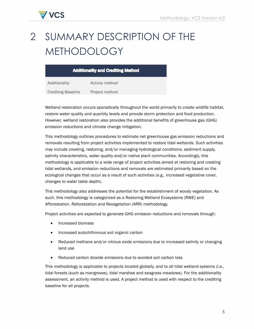
2 SUMMARY DESCRIPTION OF THE METHODOLOGY
Additionality and Crediting Method
Additionality Activity method
Crediting Baseline Project method
Wetland restoration occurs sporadically throughout the world primarily to create wildlife habitat, restore water quality and quantity levels and provide storm protection and food production. However, wetland restoration also provides the additional benefits of greenhouse gas (GHG) emission reductions and climate change mitigation.
This methodology outlines procedures to estimate net greenhouse gas emission reductions and removals resulting from project activities implemented to restore tidal wetlands. Such activities may include creating, restoring, and/or managing hydrological conditions, sediment supply, salinity characteristics, water quality and/or native plant communities. Accordingly, this methodology is applicable to a wide range of project activities aimed at restoring and creating tidal wetlands, and emission reductions and removals are estimated primarily based on the ecological changes that occur as a result of such activities (e.g., increased vegetative cover, changes to water table depth).
This methodology also addresses the potential for the establishment of woody vegetation. As such, this methodology is categorized as a Restoring Wetland Ecosystems (RWE) and Afforestation, Reforestation and Revegetation (ARR) methodology.
Project activities are expected to generate GHG emission reductions and removals through:
• Increased biomass
• Increased autochthonous soil organic carbon
• Reduced methane and/or nitrous oxide emissions due to increased salinity or changing land use
• Reduced carbon dioxide emissions due to avoided soil carbon loss
This methodology is applicable to projects located globally, and to all tidal wetland systems (i.e., tidal forests (such as mangroves), tidal marshes and seagrass meadows). For the additionality assessment, an activity method is used. A project method is used with respect to the crediting baseline for all projects.
Methodology: VCS Version 4.0
6
For strata with organic soil, this methodology sets out procedures for the estimation of peat depletion time (PDT). Likewise, for strata with mineral soils and sediments, this methodology provides procedures for the estimation of soil organic carbon depletion time (SDT). This methodology also includes an assessment of the maximum quantity of GHG emission reductions which may be claimed from the soil organic carbon (SOC) pool (either based on the difference between the remaining soil organic carbon stock in the project and baseline scenarios after 100 years (total stock approach), or the difference in cumulative carbon loss in both scenarios since the project start date (stock loss approach)).
To estimate carbon stock changes in tree and shrub biomass, this methodology uses procedures from CDM tool AR-Tool14 Estimation of carbon stocks and change in carbon stocks of trees and shrubs in A/R CDM project activities. This methodology also provides a method to account for carbon stock changes in herbaceous vegetation.
Since biomass may be lost due to subsidence following sea level rise, restoration projects involving afforestation or reforestation may account for long-term carbon storage in wood products where trees are harvested before dieback.
GHG emissions from the SOC pool are estimated by assessing emissions of CO2, CH4 and N2O, which may be estimated via several methods (e.g., proxies, modeling, default factors, local published values). Where allochthonous SOC accumulates in the project scenario, a procedure is provided to deduct such carbon from net emission reductions.
Proxies for emissions from the SOC pool may include water table depth and soil subsidence (for which procedures from other methodologies and modules are used) and carbon stock change. For non-seagrass tidal wetland systems, a default factor may be used in the absence of local data.
CH4 and N2O emissions in the baseline scenario may be conservatively set to zero. Where the project proponent demonstrates that CH4 or N2O emissions do not increase in the project scenario compared to the baseline scenario, these emissions need not be accounted for.
This methodology also addresses anthropogenic peat fires occurring in drained areas and establishes a conservative default value (Fire Reduction Premium) based on fire occurrence and extension in the project area in the baseline scenario. The procedure is based on VCS module VMD0046 Methods for monitoring soil carbon stock changes and GHG emissions in WRC project activities. The approach avoids the direct assessment of GHG emissions from fire in the baseline and project scenarios.
This methodology also includes procedures to account for GHG emissions from prescribed burning (using literature-based emission factors for non-CO2 GHGs) and fossil fuel use (by incorporating procedures from the CDM tool AR-Tool05 Estimation of GHG emissions related to fossil fuel combustion in A/R CDM project activities).
Methodology: VCS Version 4.0
7
This methodology includes procedures for the consideration of sea level rise with respect to determining the geographic boundaries of the project area, and the determination of the baseline scenario and baseline emissions.
Activity-shifting leakage and market leakage are deemed not to occur if the applicability conditions of this methodology are met. Furthermore, activity-shifting leakage and market leakage are deemed not to occur if the pre-project land use will continue during the project crediting period.
Under the applicability conditions of this methodology, ecological leakage does not occur by ensuring that the effect of hydrological connectivity with adjacent areas is insignificant (i.e., no alteration of mean annual water table depths will occur in such areas). In tidal wetland restoration projects, de-watering downstream wetlands is not expected.
This methodology provides the steps necessary for estimating the project’s net GHG benefits, as represented by the equation below:
NERRWE = GHGBSL – GHGWPS + FRP – GHGLK
Where: NERRWE = Net CO2e emission reductions from the RWE project activity GHGBSL = Net CO2e emissions in the baseline scenario GHGWPS = Net CO2e emissions in the project scenario FRP = Fire Reduction Premium (net CO2e emission reductions from organic soil combustion due to rewetting and fire management) GHGLK = Net CO2e emissions due to leakage
3 DEFINITIONS In addition to the definitions set out in VCS document Program Definitions, the following definitions apply to this methodology:
Allochthonous Soil Organic Carbon Soil organic carbon originating outside the project area and being deposited in the project area Autochthonous Soil Organic Carbon Soil organic carbon originating or forming in the project area (e.g., from vegetation) Carbon Preservation Depositional Environment (CPDE) Type of sub-aquatic sediment deposition environment that impacts the amount of deposited organic carbon that is preserved. Carbon preservation is affected by mineral grain size, sediment accumulation and burial rates, O2 availability in the overlying water column and sediment hydraulic conductivity.

Methodology: VCS Version 4.0
8
Degraded wetland A wetland which has been altered by human or natural impact through the impairment of physical, chemical and/or biological properties, and in which the alteration has resulted in a reduction of the diversity of wetland-associated species, soil carbon or the complexity of other ecosystem functions which previously existed in the wetland Deltaic Fluidized Mud A Carbon Preservation Depositional Environment (CPDE) type. This subaquatic depositional environment is characterized by sediment accumulation rates generally greater than 0.4 g sediment per cm2 per year in deltaic settings, consisting primarily of fluidized (unconsolidated) fine-grain materials. Surface sediments may be re-suspended by waves and tides, but deposited organic matter will be buried. Examples of these can be found in the Amazon and Mississippi deltas. Extreme Accumulation Rate A Carbon Preservation Depositional Environment (CPDE) type. This subaquatic depositional environment is characterized by accumulation rates generally greater than 1 g sediment per cm2 per year resulting in rapid and long-term burial of deposited sediments. Examples of these systems can be found in the Ganges-Brahmaputra and Rhone River deltas. Impounded Water A pool of water formed by a dam or pit Marsh A subset of wetlands characterized by emergent soft-stemmed vegetation adapted to saturated soil conditions1 Mineral Soil Soil that is not organic Mudflat A subset of tidal wetlands consisting of soft substrate not supporting emergent vegetation Normal marine A Carbon Preservation Depositional Environment (CPDE) type. This is a depositional environment that does not meet the definition of the other four defined conditions (i.e., deltaic fluidized mud, extreme accumulation rate, oxygen depletion zone, or small mountainous river).
1 There are many different kinds of marshes, ranging from the prairie potholes to the Everglades, coastal to inland, freshwater to saltwater, but the scope of this methodology is limited to tidal marshes. Salt marshes consist of salt-tolerant and dwarf brushwood vegetation overlying mineral or organic soils.

Methodology: VCS Version 4.0
9
Normal marine environments typically have low sedimentation rates and high O2 availability in overlying sediments. Open Water An area in which water levels do not fall to an elevation that exposes the underlying substrate Organic Soil Soil with a surface layer of material that has a sufficient depth and percentage of organic carbon to meet thresholds set by the IPCC (Wetlands supplement) for organic soil. Where used in this methodology, the term peat is used to refer to organic soil. Oxygen (O2) Depletion Zone A Carbon Preservation Depositional Environment (CPDE) type. This is a depositional environment with low O2 levels in water overlying sediments due to restricted hydrologic circulation or impaired water quality that leads to hypoxic or anaerobic conditions (including euxinic and semi-euxinic). Salinity Average The average water salinity value of a wetland ecosystem used to represent variation in salinity during periods of peak CH4 emissions (e.g., during the growing season in temperate ecosystems) Salinity Low Point The minimum water salinity value of a wetland ecosystem used to represent variation in salinity during periods of peak CH4 emissions (e.g., during the growing season in temperate ecosystems) Seagrass Meadow An accumulation of seagrass plants over a mappable area2 Small Mountainous River A Carbon Preservation Depositional Environment (CPDE) type. This is a depositional environment from which the sediment is supplied from small mountainous rivers, most commonly found in tectonically active margins and small steep gradients. Sediment accumulation rates are generally greater than 0.27 g sediment per cm2 per year. Examples of these systems can be found in the rivers flowing from the island of Taiwan and the Eel River of California. Tidal Wetland A subset of wetlands under the influence of the wetting and drying cycles of the tides (e.g., marshes, seagrass meadows, tidal forested wetlands, and mangroves). Sub-tidal seagrass
2 This definition includes both the biotic community and the geographic area where the biotic community occurs. Note that the vast majority of seagrass meadows are sub-tidal, but a percentage are intertidal.
Methodology: VCS Version 4.0
10
meadows are not subject to drying cycles but are still included in this definition. Tidal Wetland Restoration Re-establishing or improving the hydrology, salinity, water quality, sediment supply and/or vegetation in degraded or converted tidal wetlands. For the purpose of this methodology, this definition also includes activities that create wetland ecological conditions on uplands under the influence of sea level rise or activities that convert one wetland type to another or activities that convert open water to wetland. Water Table Depth Depth of sub-soil or above-soil surface of water, relative to the soil surface
4 APPLICABILITY CONDITIONS This methodology applies to tidal wetland restoration project activities (tidal wetland restoration as defined in Section 3 above) under the following applicability conditions:
1) Project activities which restore tidal wetlands (including seagrass meadows, per this methodology’s definition of tidal wetland) are eligible.
2) Project activities may include any of the following, or combinations of the following:
a) Creating, restoring and/or managing hydrological conditions (e.g., removing tidal barriers, improving hydrological connectivity, restoring tidal flow to wetlands or lowering water levels on impounded wetlands)
b) Altering sediment supply (e.g., beneficial use of dredge material or diverting river sediments to sediment-starved areas)
c) Changing salinity characteristics (e.g., restoring tidal flow to tidally restricted areas)
d) Improving water quality (e.g., reducing nutrient loads leading to improved water clarity to expand seagrass meadows, recovering tidal and other hydrologic flushing and exchange, or reducing nutrient residence time)
e) (Re-)introducing native plant communities (e.g., reseeding or replanting)
f) Improving management practice(s) (e.g., removing invasive species, reduced grazing)
3) Prior to the project start date, the project area:
a) Is free of any land use that could be displaced outside the project area, as demonstrated by at least one of the following, where relevant:
Methodology: VCS Version 4.0
11
i) The project area has been abandoned for two or more years prior to the project start date; or
ii) Use of the project area for commercial purposes (i.e., trade) is not profitable as a result of salinity intrusion, market forces or other factors. In addition, timber harvesting in the baseline scenario within the project area does not occur; or
iii) Degradation of additional wetlands for new agricultural sites within the country will not occur or is prohibited by enforced law.
OR
b) Is under a land use that could be displaced outside the project area), although in such case baseline emissions from this land use must not be accounted for, and where degradation of additional wetlands for new agricultural/aquacultural sites within the country will not occur or is prohibited by enforced law.
OR
c) Is under a land use that will continue at a similar level of service or production during the project crediting period (e.g., reed or hay harvesting, collection of fuelwood, subsistence harvesting).
The project proponent must demonstrate (a), (b) or (c) above based on verifiable information such as laws and bylaws, management plans, annual reports, annual accounts, market studies, government studies or land use planning reports and documents.
4) Live tree vegetation may be present in the project area and may be subject to carbon stock changes (e.g., due to harvesting) in both the baseline and project scenarios.
5) The prescribed burning of herbaceous and shrub aboveground biomass (cover burns) as a project activity may occur.
6) Where the project proponent intends to claim emission reductions from reduced frequency of peat fires, project activities must include a combination of rewetting and fire management.
7) Where the project proponent intends to claim emission reductions from reduced frequency of peat fires, it must be demonstrated that a threat of frequent on-site fires exists, and the overwhelming cause of ignition of the organic soil is anthropogenic (e.g., drainage of the peat, arson).
8) In strata with organic soil, afforestation, reforestation, and revegetation (ARR) activities must be combined with rewetting.
This methodology is not applicable under the following conditions:

Methodology: VCS Version 4.0
12
1) Project activities qualify as IFM or REDD.
2) Baseline activities include commercial forestry.
3) Project activities lower the water table, unless the project converts open water to tidal wetlands, or improves the hydrological connection to impounded waters.
4) Hydrological connectivity of the project area with adjacent areas leads to a significant increase in GHG emissions outside the project area.
5) Project activities include the burning of organic soil.
6) Nitrogen fertilizer(s), such as chemical fertilizer or manure, are applied in the project area during the project crediting period.
5 PROJECT BOUNDARY
5.1 Temporal Boundaries
Peat depletion time (PDT)
Drained peat is subject to oxidation and subsidence and areas with peat at t = 0 may lose all peat before the end of the crediting period. The time at which all peat has disappeared, or at which the peat depth reaches a level where no further oxidation or other losses occur (e.g., at the average water table depth), is referred to as the PDT. Projects that do not quantify reductions of baseline emissions (i.e., those which limit their accounting to GHG removals in biomass and/or soil) need not estimate PDT.
PDT (tPDT-BSL,i) for a stratum in the baseline scenario limits the period during which the project is eligible to claim soil emission reductions from rewetting, and is estimated at the project start date for each stratum i as:
tPDT-BSL,i = Depthpeat,i,t0 / Ratepeatloss-BSL,I (1)
Where: tPDT-BSL,I = PDT in the baseline scenario in stratum i (in years elapsed since the project
start date); yr Depthpeat,i,t0 = Average organic soil depth above the drainage limit in stratum i at the
project start date; m Ratepeatloss-BSL,i = Rate of organic soil loss due to subsidence and fire in the baseline scenario
in stratum i; a conservative (high) value must be applied that remains constant over the time from t = 0 to PDT; m yr-1.
i = 1, 2, 3 …MBSL strata in the baseline scenario

Methodology: VCS Version 4.0
13
If tPDT-BSL,i falls within the crediting period, subsequent organic carbon loss from remaining mineral soil may be estimated as well using the procedure for SDT in Section 5.1.2.
Organic soil depths, depths of burn scars and subsidence rates must be derived from the data sources described in Section Error! Reference source not found.. Water table depth is assessed, if relevant, following procedures in Section 9.3.11.
If tPDT-BSL,i falls within the Crediting Period, subsequent organic carbon loss from remaining mineral soil may be estimated as well using the procedure for SDT in Section 5.1.2, below.
Soil organic carbon depletion time (SDT)
Projects that do not quantify reductions of baseline emissions (i.e., those which limit their accounting to GHG removals in biomass and/or soil) need not estimate SDT.
SDT (tSDT-BSL,i) for a stratum in the baseline scenario limits the period during which the project is eligible to claim emission reductions from restoration, and is estimated at the project start date for each stratum i as follows:
For strata with eroded soils:
tSDT-BSL,i = 5 years (1)
For strata with soils exposed to an aerobic environment through excavation or drainage, use the following equation.
tSDT-BSL,i = CBSL,i,t0 / RateCloss-BSL,i (2)
Where: tSDT-BSL,i = SDT in the baseline scenario in stratum i (in years elapsed since the project start date); yr CBSL,i,t0 = Average organic carbon stock in the baseline scenario in mineral soil in stratum i at the project start date; t C ha-1 (see Equation 10) RateCloss-BSL,i = Rate of soil organic carbon loss due to oxidation in the baseline scenario in stratum i; a conservative (high) value must be applied that remains constant over the time from t = 0 to SDT; t C ha-1 yr-1. i = 1, 2, 3 … MBSL strata in the baseline scenario
The project proponent must determine the depth (Depthsoil,i,t0 in Equation 12 below) over which CBSL,i,t0 is determined. Note that a shallower depth will lead to a shorter, and more conservative, SDT. Where SDT is not determined, no reductions of baseline emissions from mineral soil may be claimed.

Methodology: VCS Version 4.0
14
Extrapolation of RateCloss-BSL,i over the project crediting period must account for the possibility of a non-linear decrease of soil organic carbon over time, including the tendency of organic carbon concentrations to approach steady-state equilibrium. For this reason, a complete loss of soil organic carbon may not occur in mineral soils. This steady-state equilibrium must be determined conservatively.
In case of alternating mineral and organic horizons, RateCloss-BSL,i may be determined for all individual horizons. This also applies to cases where an organic surface layer of less than 10 cm exists or in cases where the soil is classified as organic but its organic matter depletion is expected within the project crediting period and oxidation of organic matter in an underlying mineral soil may occur within this period.
SDT is conservatively set to zero for project sites drained more than 20 years prior to the project start date. SDT is also conservatively set to zero where significant soil erosion occurs in the baseline scenario (significant defined as >5% of RateCloss-BSL,i).
With respect to the estimation of SDT, the accretion of sediment in the baseline scenario is conservatively excluded.
5.2 Geographic Boundaries
General
The project proponent must define the geographic boundaries of the project area at the beginning of project activities. The project proponent must provide the geographic coordinates of lands (including sub-tidal seagrass areas, where relevant) included in the project area to facilitate accurate delineation of the project area. Remotely sensed data, published topographic maps and data, land administration and tenure records and/or other official documentation that facilitates clear delineation of the project area must be used.
The project activity may contain more than one discrete area of land. Each discrete area of land must have a unique geographical identification.
When describing physical project boundaries, the following information must be provided for each discrete area:
• Name of the project area (including compartment numbers, local name (if any)).
• Unique identifier for each discrete parcel of land.
• Map(s) of the area (preferably in digital format).
• The project area must be geo-referenced and provided in digital format in accordance with VCS rules.
• Total area.
• Details of land rights holder and user rights.

Methodology: VCS Version 4.0
15
Stratification
Where the project area at the project start date is not homogeneous, stratification may be carried out to improve the accuracy and the precision of carbon stock and GHG flux estimates. Where stratification is employed, different stratifications may be required for the baseline and project scenarios in order to achieve optimal accuracy of the estimates of net GHG emission reductions and removals.
Strata may be defined based on soil type and depth (including eligibility as assessed below), water table depth, vegetation cover and/or vegetation composition, salinity, land type (open water, channel, and unvegetated sand or mudflat) or expected changes in these characteristics.
Strata must be spatially discrete and stratum areas must be known. Areas of individual strata must sum to the total project area. Strata must be identified with spatial data (e.g., maps, GIS coverage, classified imagery, sampling grids) from which the area can be determined accurately. Land use/land cover maps in particular must be ground-truthed and less than 10 years old, unless it can be demonstrated that the maps are still accurate. Strata must be discernible taking into account good practice with respect to accuracy requirements for the definition of strata limits and boundaries. The type of spatial data must be indicated and justified in the project description.
The project area may be stratified ex ante, and this stratification may be revised ex post for monitoring purposes. Established strata may be merged if reasons for their separate establishment are no longer meaningful, or have proven irrelevant to key variables for estimating net GHG emission reductions and removals. Baseline stratification must remain fixed until a reassessment of the baseline scenario occurs. Stratification in the project scenario must be reviewed at each monitoring event prior to verification and revised if necessary.
The sub-sections below specify further requirements and guidance with respect to stratification in certain scenarios.
Areas with organic soil
The project proponent must use VCS module VMD0016 Methods for Stratification of the Project Areas in order to stratify project areas that include organic soil.
Seagrass meadows
Given the tendency of seagrasses to respond differently under different light and depth regimes, the project proponent may differentiate between seagrass meadow sections that occur at different depths given discrete, or relatively abrupt, bathymetric and substrate changes.
For seagrass meadow restoration projects in areas with existing seagrass meadows, the project proponent must quantify the percentage of meadow expansion that can be attributed to the restoration effort but that is not the result of direct planting or seeding. Existing meadows
Methodology: VCS Version 4.0
16
(unless smaller in area than 5% of the total project area) must be excluded from the calculation of project emissions, even in cases where the restored meadow enhances carbon sequestration rates in existing meadows.
New seagrass meadows that result from natural expansion must be contiguous with restored meadow plots in order to be included in project accounting, unless the project proponent demonstrates that non-contiguous meadow patches originated from restored meadow seeds. This may be performed via genetic testing or estimated as a percentage of new meadow in non-contiguous plots and observed no less than four years after the project start date.3 This percentage must not exceed the proportion of restored meadow area relative to the total extent of seagrass meadow areal, and the project proponent must demonstrate the feasibility of current-borne seed dispersal from the restored meadow. In cases where a restored meadow coalesces with an existing meadow(s), the project proponent must delineate the line at which the two meadows are joined. The project proponent may use either aerial observations showing meadow extent or direct field observations.
Native ecosystems
In order to claim emission removals from ARR or WRC activities, the project proponent must provide evidence in the project description that the project area was not cleared of native ecosystems to create GHG credits. Such proof is not required where such clearing took place prior to the 10-year period prior to the project start date. Areas that do not meet this requirement must be excluded from the project area.
Stratification of vegetation cover for adoption of the default SOC accumulation rate
The default factor for SOC accumulation rate may only be applied to non-seagrass tidal wetland systems with a crown or vegetation cover of at least 15%, with a linearly discounted factor for areas with a crown or vegetation cover of less than 50% (see Sections 8.1.4.2.3 and 8.2.4.2.1). For the baseline scenario, crown or vegetation covers must be based on a time series of vegetation composition. For the project scenario, crown or vegetation cover mapping must be performed according to established methods in scientific literature.
Stratification of salinity for the accounting of CH4
Tidal wetlands may be stratified according to salinity for the purpose of estimating CH4 emissions. Threshold values of salinity for mapping salinity strata are specified in Section 8.1.4.5.4.
Areas with unrestricted tidal exchange will maintain salinity levels similar to the tidal water source, while those with infrequent tidal flooding will not (in which case the use of channel water salinity levels is not reliable). For such areas it is therefore recommended to stratify according to the frequency of tidal exchange.
3 McGlathery et al. (2012)

Methodology: VCS Version 4.0
17
Procedures for the measurement of salinity levels are specified in Section 9.3.8.
Stratification of water bodies lacking tidal exchange
The area of ponds, ditches or similar bodies of water within the project area must be measured and treated as separate strata when they do not have surface tidal water exchange. CH4 emissions from these features may be excluded from GHG accounting if the area of these features does not increase in the project scenario.
Sea level rise
When defining geographic project boundaries and strata, the project proponent must consider expected relative sea level rise and the potential for expanding the project area landward to account for wetland migration, inundation and erosion. The project area cannot be changed during the project crediting period.
For both the baseline and project scenarios, the project proponent must provide a projection of relative sea level rise within the project area based on IPCC regional forecasts or peer-reviewed literature applicable to the region. In addition, the project proponent may also utilize expert judgment4. Global average sea level rise scenarios are not suitable for determining the changes in wetlands boundaries. Therefore, if used, IPCC most-likely global sea level rise scenarios must be appropriately downscaled to regional conditions that include vertical land movements, such as subsidence.
Whether degradation occurs in the baseline scenario or restoration occurs in the project scenario, the assessment of potential wetland migration, inundation and erosion with respect to projected sea level rise must account for topographical slope, land use and management, sediment supply and tidal range. The assessment may use published data from the project area, expert judgment or both.
When assessing the potential for tidal wetlands to migrate horizontally, one must consider the topography of the adjacent land and any migration barriers that may exist. In general, and on coastlines where wetland migration is unimpaired by infrastructure, concave-up slopes may cause ‘coastal squeeze’, while straight or convex-up gradients are more likely to provide the space required for lateral movement.
The potential for tidal wetlands to rise vertically with sea level rise is sensitive to suspended sediment loads in the system. A sediment load of >300 mg/l has been found to balance high-end IPCC scenarios for sea level rise (Orr et al. 2003, Stralsburg et al. 2011). French (2006) and Morris et al. (2012) suggest that the findings of Orr et al. 2003 from the San Francisco Bay could be used elsewhere5. French (2006) indicates that at 250 mg/l, sea level rise of 15 mm is balanced at a tidal range of 1 m or greater. Therefore, for marshes with a tidal range
4 Requirements for expert judgment are provided in Section 9.3.3. 5 Orr et al. 2003, Stralberg et al. 2011

Methodology: VCS Version 4.0
18
greater than 1 m, the project proponent may use >300 mg/l as a sediment load threshold above which wetlands are not predicted to be submerged. The project proponent may use lower threshold values for tidal range and sediment load where justified. The vulnerability of tidal wetlands to sea level rise and conversion to open water is also related to tidal range. In general, the most vulnerable tidal wetlands are those in areas with a small tidal range, those with elevations low in the tidal frame and those in locations with low suspended sediment loads.
Alternatively, in the project scenario the project proponent may conservatively assume that part of the wetland within the project area erodes and does not migrate. See Section 8.1.4.3 for procedures to estimate CO2 emissions from eroded soil. In the baseline scenario, the project proponent may conservatively assume that part of the project area submerges, with cessation of GHG removal from the atmosphere as a consequence. If the project is not claiming emissions due to erosion in the baseline scenario, the project proponent may conservatively assume that part of the project area erodes. For areas that submerge without erosion, the loss of SOC may be assumed to be insignificant in both the baseline and project scenarios.
The projection of wetland boundaries within the project area must be presented in maps delineating these boundaries from the project start date until the end of the project crediting period, at intervals appropriate to the rate of change due to sea level rise, and at t = 100.
Procedures for accounting for project area submergence due to relative sea level rise are provided in Section 8.2.2.
Estimation of area of eroded strata
Tidal wetlands may be subject to two forms of erosion: a) Seaward edges of wetlands are subject to migration due to changes in local sea level, regional sediment delivery, and impacts of human actions (e.g., nearby excavation of shipping channels); b) In sheltered settings, away from open shores, wetlands may also erode internally through channel enlargement if sediment supply for wetland accretion is insufficient to keep pace with sea-level rise.
Projections of future erosion must take into account scaling of wetland retreat against projections of accelerated sea-level rise, any modification to sediment supply and human action.
Channel densities (surface area of channel per surface area of wetland) greater than 20% and/or changes in wetland vegetation consistent with increased duration or depth of flooding is an indication that the wetland may not be keeping pace with sea level. Similarly, a decline in surface elevation relative to a datum of mean high water surface spring elevation in the interior of the tidal wetland is an indication of wetland sensitivity to sediment supply under conditions of sea-level rise. Sites with an annual average suspended sediment load in flooding waters of >300 mg/l may be considered resilient to sea-level rise in terms of surface accretion. The project proponent should take into these indicators of wetland potential sensitivity to sea-level rise when considering whether to extend the eroded area strata to include marsh interior.
Methodology: VCS Version 4.0
19
Because such projections are driven by conditions specific to individual project settings, expert knowledge from an experienced geomorphologist / coastal engineer must be utilized for complex projects.
Ineligible wetland areas
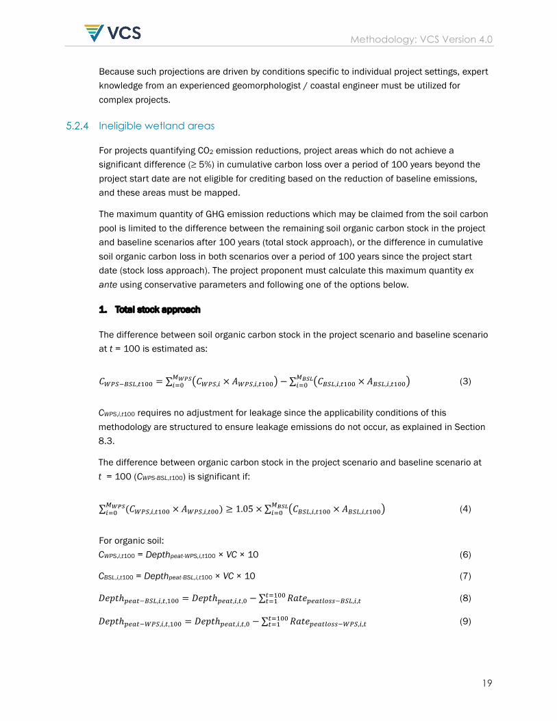
For projects quantifying CO2 emission reductions, project areas which do not achieve a significant difference (≥ 5%) in cumulative carbon loss over a period of 100 years beyond the project start date are not eligible for crediting based on the reduction of baseline emissions, and these areas must be mapped.
The maximum quantity of GHG emission reductions which may be claimed from the soil carbon pool is limited to the difference between the remaining soil organic carbon stock in the project and baseline scenarios after 100 years (total stock approach), or the difference in cumulative soil organic carbon loss in both scenarios over a period of 100 years since the project start date (stock loss approach). The project proponent must calculate this maximum quantity ex ante using conservative parameters and following one of the options below.
1. Total stock approach
The difference between soil organic carbon stock in the project scenario and baseline scenario at t = 100 is estimated as:
𝐶!"#$%#&,()** = ∑ $𝐶!"#,+ × 𝐴!"#,+,()**',!"#+-* −∑ $𝐶%#&,+,()** × 𝐴%#&,+,()**'
,$#%+-* (3)
CWPS,i,t100 requires no adjustment for leakage since the applicability conditions of this methodology are structured to ensure leakage emissions do not occur, as explained in Section 8.3.
The difference between organic carbon stock in the project scenario and baseline scenario at t = 100 (CWPS-BSL,t100) is significant if:
∑ (𝐶!"#,+,()** × 𝐴!"#,+,(**),!"#+-* ≥ 1.05 × ∑ $𝐶%#&,+,()** × 𝐴%#&,+,()**'
,$#%+-* (4)
For organic soil: CWPS,i,t100 = Depthpeat-WPS,i,t100 × VC × 10 (6)
CBSL,i,t100 = Depthpeat-BSL,i,t100 × VC × 10 (7)
𝐷𝑒𝑝𝑡ℎ./0($%#&,+,(,)** = 𝐷𝑒𝑝𝑡ℎ./0(,+,(,* −∑ 𝑅𝑎𝑡𝑒./0(1233$%#&,+,((-)**(-) (8)
𝐷𝑒𝑝𝑡ℎ./0($!"#,+,(,)** = 𝐷𝑒𝑝𝑡ℎ./0(,+,(,* −∑ 𝑅𝑎𝑡𝑒./0(1233$!"#,+,((-)**(-) (9)
Methodology: VCS Version 4.0
20
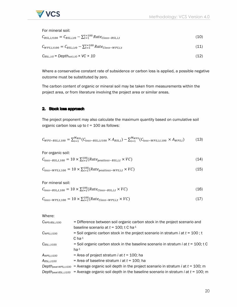
For mineral soil: 𝐶%#&,+,()** = 𝐶%#&,+,(* − ∑ 𝑅𝑎𝑡𝑒41233$%#&,+,((-)**
(-) (10)
𝐶!"#,+,()** = 𝐶%#&,+,(* −∑ 𝑅𝑎𝑡𝑒41233$!"#,+,((-)**(-) (11)
CBSL,i,t0 = Depthsoil,i,t0 × VC × 10 (12)
Where a conservative constant rate of subsidence or carbon loss is applied, a possible negative outcome must be substituted by zero.
The carbon content of organic or mineral soil may be taken from measurements within the project area, or from literature involving the project area or similar areas.
2. Stock loss approach
The project proponent may also calculate the maximum quantity based on cumulative soil organic carbon loss up to t = 100 as follows:
𝐶!"#$%#&,(,)** = ∑ (𝐶1233$%#&,+,()**,$#%+-) × 𝐴%#&,+) − ∑ (𝐶1233$!"#,+,(,)**
,!"#+-) × 𝐴!"#,+) (13)
For organic soil: 𝐶1233$%#&,(,)** = 10 × ∑ (𝑅𝑎𝑡𝑒./0(1233$%#&,+,()**
+-) × 𝑉𝐶) (14)
𝐶1233$!"#,(,)** = 10 × ∑ (𝑅𝑎𝑡𝑒./0(1233$!"#,+,()**+-) × 𝑉𝐶) (15)
For mineral soil: 𝐶1233$%#&,(,)** = 10 × ∑ (𝑅𝑎𝑡𝑒41233$%#&,+,()**
+-) × 𝑉𝐶) (16)
𝐶1233$!"#,(,)** = 10 × ∑ (𝑅𝑎𝑡𝑒41233$!"#,+,()**+-) × 𝑉𝐶) (17)
Where: CWPS-BSL,t100 = Difference between soil organic carbon stock in the project scenario and baseline scenario at t = 100; t C ha-1 CWPS,i,t100 = Soil organic carbon stock in the project scenario in stratum i at t = 100 ; t C ha-1 CBSL,i,t100 = Soil organic carbon stock in the baseline scenario in stratum i at t = 100; t C
ha-1 AWPS,i,t100 = Area of project stratum i at t = 100; ha ABSL,i,t100 = Area of baseline stratum i at t = 100; ha Depthpeat-WPS,i,t100 = Average organic soil depth in the project scenario in stratum i at t = 100; m Depthpeat-BSL,i,t100 = Average organic soil depth in the baseline scenario in stratum i at t = 100; m

Methodology: VCS Version 4.0
21
VC = Volumetric organic carbon content in organic or mineral soil; kg C m-3 Depthpeat,i,t0 = Average organic soil depth above the drainage limit in stratum i at the project
start date; m Ratepeatloss-BSL,i,t = Rate of organic soil loss due to subsidence and fire in the baseline scenario
in stratum i in year t; m yr-1. Ratepeatloss,WPS,i,t = Rate of organic soil loss due to subsidence in the project scenario in stratum
i in year t; m yr-1. CBSL,i,t0 = Soil organic carbon stock in the baseline scenario in mineral soil in stratum i
at the project start date; t C ha-1 RateCloss-BSL,i,t = Rate of organic carbon loss in mineral soil due to oxidation in the baseline
scenario in stratum i in year t; t C ha-1 yr-1. RateCloss,WPS,i,t = Rate of organic carbon loss in mineral soil due to oxidation in the project
scenario in stratum i in year t; t C ha-1 yr-1. This value is conservatively set to zero as loss rates are likely to be negative. This parameter must be reassessed when the baseline is reassessed.
Depthsoil,i,t0 = Mineral soil depth in stratum i at the project start date (as in Equation 12); m Closs-BSL,i,t100 Cumulative soil organic carbon loss in the baseline scenario in stratum i at t = 100; t C ha-1 Closs-WPS,i,t100 = Cumulative soil organic carbon loss in the project scenario in stratum i at t = 100; t C ha-1 i = 1, 2, 3 …MBSL strata in the baseline scenario t100 = 100 years after the project start date
Buffer zones
Where established, buffer zones must be mapped in accordance with the VCS rules.
5.3 Carbon Pools
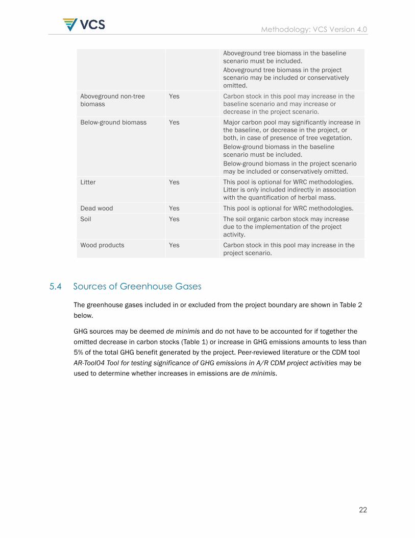
The carbon pools included in and excluded from the project boundary are shown in Table 1 below.
Carbon pools may be deemed de minimis and do not need to be accounted for if together the omitted decrease in carbon stocks or increase in GHG emissions (Table 2) amounts to less than 5% of the total GHG benefit generated by the project. Peer reviewed literature or the CDM tool AR-Tool04 Tool for testing significance of GHG emissions in A/R CDM project activities may be used to determine whether decreases in carbon pools are de minimis.
Table 1: Selection and justification of carbon pools
Carbon Pool Included? Justification/Explanation
Aboveground tree biomass Yes Major carbon pool may significantly increase or decrease in both the baseline and project scenarios, in the case of establishment or presence of tree vegetation.
Methodology: VCS Version 4.0
22
Aboveground tree biomass in the baseline scenario must be included. Aboveground tree biomass in the project scenario may be included or conservatively omitted.
Aboveground non-tree biomass
Yes Carbon stock in this pool may increase in the baseline scenario and may increase or decrease in the project scenario.
Below-ground biomass Yes Major carbon pool may significantly increase in the baseline, or decrease in the project, or both, in case of presence of tree vegetation. Below-ground biomass in the baseline scenario must be included. Below-ground biomass in the project scenario may be included or conservatively omitted.
Litter Yes This pool is optional for WRC methodologies. Litter is only included indirectly in association with the quantification of herbal mass.
Dead wood Yes This pool is optional for WRC methodologies. Soil Yes The soil organic carbon stock may increase
due to the implementation of the project activity.
Wood products Yes Carbon stock in this pool may increase in the project scenario.
5.4 Sources of Greenhouse Gases
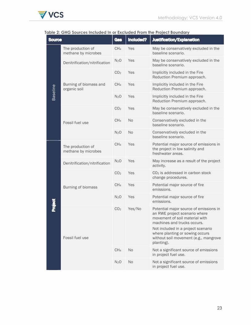
The greenhouse gases included in or excluded from the project boundary are shown in Table 2 below.
GHG sources may be deemed de minimis and do not have to be accounted for if together the omitted decrease in carbon stocks (Table 1) or increase in GHG emissions amounts to less than 5% of the total GHG benefit generated by the project. Peer-reviewed literature or the CDM tool AR-Tool04 Tool for testing significance of GHG emissions in A/R CDM project activities may be used to determine whether increases in emissions are de minimis.
Methodology: VCS Version 4.0
23
Table 2: GHG Sources Included In or Excluded From the Project Boundary
Source Gas Included? Justification/Explanation
Base
line
The production of methane by microbes
CH4 Yes May be conservatively excluded in the baseline scenario.
Denitrification/nitrification N2O Yes May be conservatively excluded in the baseline scenario.
Burning of biomass and organic soil
CO2 Yes Implicitly included in the Fire Reduction Premium approach.
CH4 Yes Implicitly included in the Fire Reduction Premium approach.
N2O Yes Implicitly included in the Fire Reduction Premium approach.
Fossil fuel use
CO2 Yes May be conservatively excluded in the baseline scenario.
CH4 No Conservatively excluded in the baseline scenario.
N2O No Conservatively excluded in the baseline scenario.
Proj
ect
The production of methane by microbes
CH4 Yes Potential major source of emissions in the project in low salinity and freshwater areas.
Denitrification/nitrification N2O Yes May increase as a result of the project activity.
Burning of biomass
CO2 Yes CO2 is addressed in carbon stock change procedures.
CH4 Yes Potential major source of fire emissions.
N2O Yes Potential major source of fire emissions.
Fossil fuel use
CO2 Yes/No Potential major source of emissions in an RWE project scenario where movement of soil material with machines and trucks occurs. Not included in a project scenario where planting or sowing occurs without soil movement (e.g., mangrove planting).
CH4 No Not a significant source of emissions in project fuel use.
N2O No Not a significant source of emissions in project fuel use.
Methodology: VCS Version 4.0
24
6 BASELINE SCENARIO 6.1 Determination of the Most Plausible Baseline Scenario
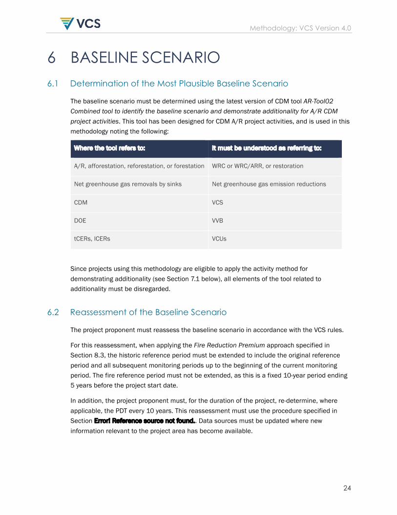
The baseline scenario must be determined using the latest version of CDM tool AR-Tool02 Combined tool to identify the baseline scenario and demonstrate additionality for A/R CDM project activities. This tool has been designed for CDM A/R project activities, and is used in this methodology noting the following:
Since projects using this methodology are eligible to apply the activity method for demonstrating additionality (see Section 7.1 below), all elements of the tool related to additionality must be disregarded.
6.2 Reassessment of the Baseline Scenario
The project proponent must reassess the baseline scenario in accordance with the VCS rules.
For this reassessment, when applying the Fire Reduction Premium approach specified in Section 8.3, the historic reference period must be extended to include the original reference period and all subsequent monitoring periods up to the beginning of the current monitoring period. The fire reference period must not be extended, as this is a fixed 10-year period ending 5 years before the project start date.
In addition, the project proponent must, for the duration of the project, re-determine, where applicable, the PDT every 10 years. This reassessment must use the procedure specified in Section Error! Reference source not found.. Data sources must be updated where new information relevant to the project area has become available.
Where the tool refers to: It must be understood as referring to:
A/R, afforestation, reforestation, or forestation WRC or WRC/ARR, or restoration
Net greenhouse gas removals by sinks Net greenhouse gas emission reductions
CDM VCS
DOE VVB
tCERs, lCERs VCUs
Methodology: VCS Version 4.0
25
7 ADDITIONALITY This methodology uses an activity method for the demonstration of additionality of tidal wetlands conservation and restoration project activities. For such project activities, use Module VDM0052 Demonstration of Additionality of Tidal Wetland Restoration and Conservation Project Activities.
8 QUANTIFICATION OF GHG EMISSION REDUCTIONS AND REMOVALS
8.1 Baseline Emissions
General approach
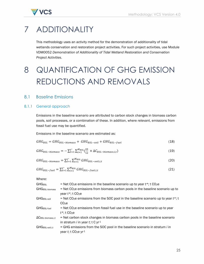
Emissions in the baseline scenario are attributed to carbon stock changes in biomass carbon pools, soil processes, or a combination of these. In addition, where relevant, emissions from fossil fuel use may be quantified.
Emissions in the baseline scenario are estimated as:
𝐺𝐻𝐺%#& = 𝐺𝐻𝐺%#&$6+27033 +𝐺𝐻𝐺%#&$32+1 + 𝐺𝐻𝐺%#&$89/1
(18)
𝐺𝐻𝐺%#&$6+27033 = −∑ ∑ (::);
,$#%+-)
(∗(-) × ∆𝐶%#&$6+27033,+,()
(19)
𝐺𝐻𝐺%#&$6+27033 = ∑ ∑ 𝐺𝐻𝐺%#&$32+1,+,(,$#%+-)
(∗(-)
(20)
𝐺𝐻𝐺%#&$89/1 = ∑ ∑ 𝐺𝐻𝐺%#&$89/1,+,(,$#%+-)
(∗(-)
(21)
Where: GHGBSL = Net CO2e emissions in the baseline scenario up to year t*; t CO2e GHGBSL-biomass = Net CO2e emissions from biomass carbon pools in the baseline scenario up to
year t*; t CO2e GHGBSL-soil = Net CO2e emissions from the SOC pool in the baseline scenario up to year t*; t CO2e GHGBSL-fuel = Net CO2e emissions from fossil fuel use in the baseline scenario up to year t*; t CO2e ΔCBSL-biomass,i,t = Net carbon stock changes in biomass carbon pools in the baseline scenario in stratum i in year t; t C yr-1 GHGBSL-soil,i,t = GHG emissions from the SOC pool in the baseline scenario in stratum i in year t; t CO2e yr-1

Methodology: VCS Version 4.0
26
GHGBSL-fuel,i,t = GHG emissions from fossil fuel use the baseline scenario in stratum i in year t; tCO2e yr-1
i = 1, 2, 3 …MBSL strata in the baseline scenario t = 1, 2, 3, … t* years elapsed since the project start date
Estimation of GHG emissions and removals related to the biomass pool is based on carbon stock changes. Estimation of GHG emissions and removals from the SOC pool is based on either various proxies (e.g., carbon stock change, water table depth) or through the use of literature, data, default factors or models.
Assessing GHG emissions in the baseline scenario consists of determining GHG emission proxies/parameters and assessing their pre-project spatial distribution, constructing a time series of the chosen proxies/parameters for each stratum for the entire project crediting period and determining annual GHG emissions per stratum for the entire project crediting period.
In order to project the future GHG emissions per unit area in each stratum for each projected verification date within the project crediting period under the baseline scenario, the project proponent must apply the latest version of VCS module VMD0019 Methods to Project Future Conditions.6 When applying Steps 13 and 14 of VMD0019 (version 1, issued 16 November 2012, the version of the module current as of the writing of this methodology) the project proponent must use the guidance for sea level rise provided in Section 5.2 of this methodology.
Four driving factors are likely to be relevant for GHG accounting in the baseline scenario, and are relevant for use of VMD0019. Each factor affects the evolution of the site over a 100-year period. These include:
• Initial land use and development patterns
• Initial infrastructure that impedes natural tidal hydrology
• Natural plant succession for the physiographic region of the project
• Climate variables as likely drivers of changes in tidal hydrology within the 100-year timeframe of the project, influencing sea level rise, precipitation and associated freshwater delivery
Land use and development patterns – In order to derive trends in land use, assumptions about the likelihood of future development of the project area must be documented and considered in light of current zoning, regulatory constraints to development, proximity to urban areas or transportation infrastructure, and expected population growth, including how land would
6 This module provides detailed procedures for assessing future trends in key variables that affect GHG emissions or removals. In the context of this methodology, this module is meant to assist in the assessment of these trends and does not necessarily replace procedures in this methodology. Procedures in the module must be used whenever relevant and may be justifiably simplified.
Methodology: VCS Version 4.0
27
develop within and surrounding the project site and how such changes would change hydrologic conditions within the project area. Current development patterns and plausible future land use changes must be mapped to a scale sufficient to estimate GHG emissions from the baseline scenario. Particular attention must be paid to existing or future construction of barriers to tidal and/or river hydrology and sediment supply from rivers and/or along the coast, as well as barriers that will impair wetland capacity to migrate landwards with sea level rise. In the case of abandonment of pre-project land use in the baseline scenario, the project proponent must consider non-human induced hydrologic changes brought about by collapsing dikes or ditches that would have naturally closed over time, and progressive subsidence, leading to rising relative water levels, increasingly thinner aerobic layers and reduced CO2 emission rates.
Infrastructure impediments to tidal hydrology – In order to derive trends in tidal wetland evolution, the baseline scenario must take into account the current and historic layout of any tidal barriers and drainage systems. The tidal barriers and drainage layout at the start of the project activity must be mapped at scale (1:10,000 or any other scale justified for estimating water table depths throughout the project area). Historic tidal barriers and drainage layout must be mapped using topographic and/or hydrological maps from (if available) the start of the major hydrological impacts but covering at least the 20 years prior to the project start date. Historic drainage structures (collapsed ditches) may (still) have higher hydraulic conductivity than the surrounding areas and function as preferential flow paths. Historic tidal barriers (agricultural dikes and levees) may constrain the tidal flows and prevent natural sedimentation patterns. The effect of historic tidal barriers and drainage structures on current hydrological functioning of the project area must be assessed on the basis of quantitative hydrological modeling and/or expert judgment.
Historic information on the pre-existing channel network as determined by aerial photography may serve to set trends in post-project dendritic channel formation in the field. Derivation of such trends must be performed on the basis of hydrologic modeling using the total tidal volume, soil erodibility and/or expert judgment. With respect to hydrological functioning, the baseline scenario must be restricted by climate variables and quantify any impacts on the hydrological functioning as caused by planned measures outside the project area (e.g., dam construction or further changes in hydrology such as culverts), by demonstrating a hydrological connection to the planned measures.
Natural plant succession - Based on the assessment of changes in water table depth, a time series of vegetation composition must be derived ex ante, based on vegetation succession schemes in the baseline scenario from scientific literature or expert judgment. For example, diked agricultural land will undergo natural plant succession to forests, freshwater wetlands, tidal wetlands, rank uplands, or open water based on the scenario’s land use trajectory, inundation scenario, proximity to native or invasive seed sources, plant succession trajectories of adjacent natural areas or likely maintenance consistent with projected future human land use (e.g., pasture, lawn, landscaping).

Methodology: VCS Version 4.0
28
Climate variables – Consistent with the sea level rise guidance provided in Section 5.2 above, areas of inundation and erosion within the project area must be considered in relation to the above three factors. Expected changes in freshwater delivery associated with changes in rainfall patterns must be considered, including expected human responses to these changes.
The project proponent must, for the duration of the project crediting period, reassess the baseline scenario every 10 years. Based on the reassessment criteria specified in Section 6 above, the revised baseline scenario must be incorporated into revised estimates of baseline emissions. This baseline reassessment must include the evaluation of the validity of proxies for GHG emissions.
Accounting for sea level rise
The consequences of submergence of a given stratum due to sea level rise are:
1) Carbon stocks from aboveground biomass are lost to oxidation, and
2) Depending upon the geomorphic setting, soil carbon stocks may be held intact or be eroded and transported beyond the project area.
For strata where conversion to open water is expected before t = 100, the maximum quantity of GHG emission reductions that may be claimed by the project must be calculated as defined in Section 8.5.1.
Regarding (1) above, where biomass is submerged, it is assumed that this carbon is immediately and entirely returned to the atmosphere. For such strata:
ΔCBSL-agbiomass,i,t = 12/44 × (CBSL-agbiomass,i,t – CBSL-agbiomass,i,(t-T)) / T
(22)
For the year of submergence: CBSL-agbiomass,i,t = 0
Where: ΔCBSL-agbiomass,i,t = Net carbon stock change in aboveground biomass carbon pools in the baseline
scenario in stratum i in year t; t C yr-1 CBSL-agbiomass,i,t = Carbon stock in aboveground biomass in the baseline scenario in stratum i in year t (from the aboveground biomass components in CTREE_BSL,t and CSHRUB_BSL,t in AR-Tool14 and CBSL-herb,i,t); t CO2e i = 1, 2, 3 …MBSL strata in the baseline scenario t = 1, 2, 3, … t* years elapsed since the project start date T = Time elapsed between two successive estimations (T=t2 – t1)
The gradual loss of vegetation in the project area due to submergence may be captured by detailed stratification into areas with and without vegetation.
Methodology: VCS Version 4.0
29
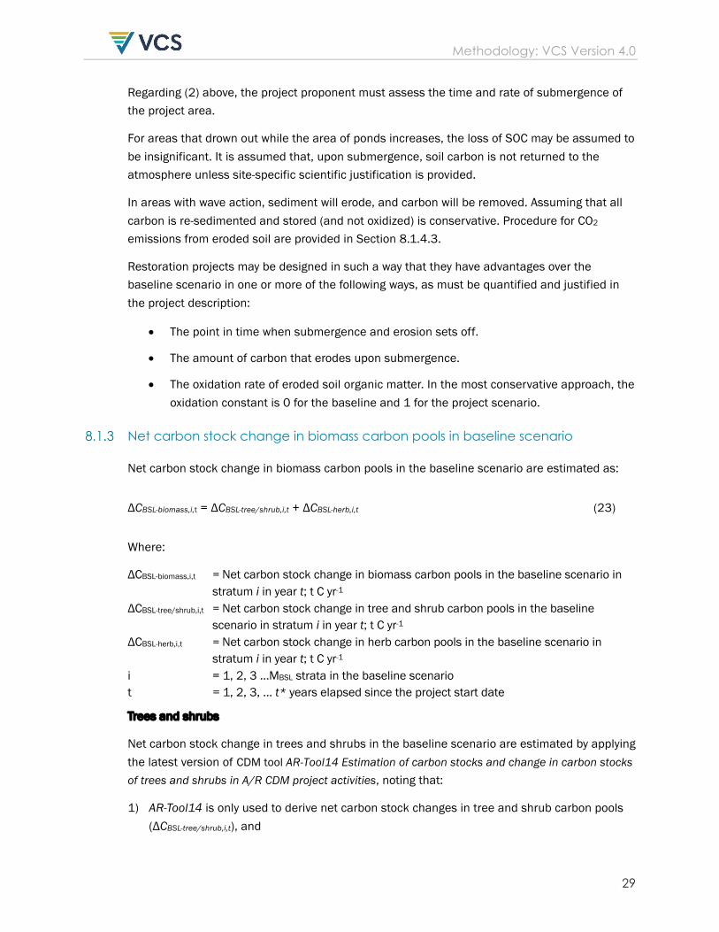
Regarding (2) above, the project proponent must assess the time and rate of submergence of the project area.
For areas that drown out while the area of ponds increases, the loss of SOC may be assumed to be insignificant. It is assumed that, upon submergence, soil carbon is not returned to the atmosphere unless site-specific scientific justification is provided.
In areas with wave action, sediment will erode, and carbon will be removed. Assuming that all carbon is re-sedimented and stored (and not oxidized) is conservative. Procedure for CO2 emissions from eroded soil are provided in Section 8.1.4.3.
Restoration projects may be designed in such a way that they have advantages over the baseline scenario in one or more of the following ways, as must be quantified and justified in the project description:
• The point in time when submergence and erosion sets off.
• The amount of carbon that erodes upon submergence.
• The oxidation rate of eroded soil organic matter. In the most conservative approach, the oxidation constant is 0 for the baseline and 1 for the project scenario.
Net carbon stock change in biomass carbon pools in baseline scenario
Net carbon stock change in biomass carbon pools in the baseline scenario are estimated as:
ΔCBSL-biomass,i,t = ΔCBSL-tree/shrub,i,t + ΔCBSL-herb,i,t (23)
Where:
ΔCBSL-biomass,i,t = Net carbon stock change in biomass carbon pools in the baseline scenario in stratum i in year t; t C yr-1 ΔCBSL-tree/shrub,i,t = Net carbon stock change in tree and shrub carbon pools in the baseline scenario in stratum i in year t; t C yr-1 ΔCBSL-herb,i,t = Net carbon stock change in herb carbon pools in the baseline scenario in stratum i in year t; t C yr-1 i = 1, 2, 3 …MBSL strata in the baseline scenario t = 1, 2, 3, … t* years elapsed since the project start date
Trees and shrubs
Net carbon stock change in trees and shrubs in the baseline scenario are estimated by applying the latest version of CDM tool AR-Tool14 Estimation of carbon stocks and change in carbon stocks of trees and shrubs in A/R CDM project activities, noting that:
1) AR-Tool14 is only used to derive net carbon stock changes in tree and shrub carbon pools (ΔCBSL-tree/shrub,i,t), and
Methodology: VCS Version 4.0
30
2) The following equation applies:
ΔCBSL-tree/shrub,i,t = 12/44 × (ΔCTREE_BSL,t + ΔCSHRUB_BSL,t) (24)
Where: ΔCBSL-tree/shrub,i,t = Net carbon stock changes in tree and shrub carbon pools in the baseline
scenario in stratum i in year t; t C yr-1 ΔCTREE_BSL,t = Change in carbon stock in baseline tree biomass within the project area in
year t; t CO2-e yr-1 (derived from application of AR-Tool14; calculations are done for each stratum i)
ΔCSHRUB_BSL,t = Change in carbon stock in baseline shrub biomass within the project area in year t; t CO2-e yr-1 (derived from application of AR-Tool14; calculations are done
for each stratum i)
For strata where reforestation or revegetation activities in the baseline scenario include harvesting, the long-term average of CTREE_BSL,t in AR-Tool14 must be calculated as specified in Section 8.2.3.
Herbaceous vegetation
Net carbon stock change in herbaceous vegetation in the baseline scenario is estimated using a carbon stock change approach as follows:
ΔCBSL-herb,i,t = (CBSL-herb,i,t – CBSL-herb,i,,(t-T)) / T
(25)
Where: ΔCBSL-herb,i,t = Net carbon stock change in herbaceous vegetation carbon pools in the
baseline scenario in stratum i in year t; t C yr-1 CBSL-herb,i,t = Carbon stock in herbaceous vegetation in the baseline scenario in stratum i in year t; t C i = 1, 2, 3 …MBSL strata in the baseline scenario t = 1, 2, 3 … t* years elapsed since the project start date T = Time elapsed between two successive estimations (T=t2 – t1)
A default factor7 for carbon stock in herbaceous vegetation of 3 t C ha-1 may be applied for strata with 100% herbaceous cover. For areas with a vegetation cover <100%, a 1:1 relationship between vegetation cover and carbon stock must be applied. The default factor may be claimed only for the first year of the project crediting period as herbaceous biomass
7 Calculated from peak aboveground biomass data from 20 sites summarized in Mitsch & Gosselink. The median of these studies is 1.3 kg d.m. m-2. This was converted to the default factor value as follows: 1.3 × 0.45 × 0.5. The factor 0.45 converts organic matter mass to carbon mass; the factor 0.5 is a factor that averages annual peak biomass (factor = 1) and annual minimum biomass (factor = 0, assuming ephemeral aboveground biomass and complete litter decomposition).

Methodology: VCS Version 4.0
31
quickly reaches a steady state. Vegetation cover must be determined by commonly used techniques in field biology. Procedures for measuring carbon stocks in herbaceous vegetation are provided in Section 9.3.6. The above default factor may not be applied in case AR-Tool14 is used.
Where a carbon stock increase in herbaceous vegetation is quantified in the project scenario, carbon stock changes must also be quantified in the baseline scenario; where a carbon stock decline is quantified in the baseline scenario, carbon stock changes must also be quantified in the project scenario.
Net GHG emissions from soil in baseline scenario
General
Net GHG emissions from soil in the baseline scenario are estimated as:
GHGBSL-soil,i,t = Ai,t × (GHGBSL-soil-CO2,i,t - Deductionalloch + GHGBSL-soil-CH4,i,t + GHGBSL-soil-N2O,i,t) (26)
For organic soils where t > tPDT-BSL,i: GHGBSL-soil,i,t = 0
For mineral soils where t > tSDT-BSL,i: GHGBSL-soil,i,t = 0
Where: GHGBSL-soil,i,t = GHG emissions from the SOC pool in the baseline scenario in stratum i in year t; t CO2e yr-1 GHGBSL-soil-CO2,i,t = CO2 emissions from the SOC pool in the baseline scenario in stratum i in year t; t CO2e ha-1 yr-1 Deductionalloch = Deduction from CO2 emissions from the SOC pool to account for the percentage of the carbon stock that is derived from allochthonous soil organic carbon; t CO2e ha-1 yr-1 GHGBSL-soil-CH4,i,t = CH4 emissions from the SOC pool in the baseline scenario in stratum i in year t; t CO2e ha-1 yr-1 GHGBSL-soil-N2O,i,t = N2O emissions from the SOC pool in the baseline scenario in stratum i in year t; t CO2e ha-1 yr-1 Ai,t = Area of stratum i in year t; ha tPDT-BSL,i = Peat depletion time in the baseline scenario in stratum i in years elapsed since the project start date; yr tSDT-BSL,i = Soil organic carbon depletion time in the baseline scenario in stratum i in years elapsed since the project start date; yr i = 1, 2, 3 …MBSL strata in the baseline scenario t = 1, 2, 3, … t* years elapsed since the project start date
CO2 emissions from the SOC pool in the baseline scenario may occur in situ or indirectly following soil erosion or exposure to an aerobic environment through excavation as defined in
Methodology: VCS Version 4.0
32
Equation 27. For strata with in-situ emissions (with or without drainage), follow procedures in Section 8.1.4.2. For strata where soil erosion occurs, procedures in Section 8.1.4.3 must be used. For strata where soil is exposed to an aerobic environment through excavation, procedures in Section 8.1.4.4 must be used. For strata with in-situ emissions, CH4 and N2O emissions may be conservatively set to zero or may be estimated using procedures in Sections 8.1.4.5 and 8.1.4.6, respectively. For strata where soil erosion occurs, or soil is exposed to an aerobic environment through excavation or drainage, CH4 and N2O emissions are conservatively set to zero.
GHGBSL-soil-CO2,i,t = GHGBSL-insitu-CO2,i,t + GHGBSL-eroded-CO2,i,t + GHGBSL-excav-CO2,i,t (27)
Where: GHGBSL-soil-CO2,i,t CO2 emissions from the SOC pool in the baseline scenario in stratum i in
year t; t CO2e ha-1 yr-1 GHGBSL-insitu-CO2,i,t CO2 emissions from the SOC pool of in-situ soils in the baseline scenario in
stratum i in year t; t CO2e ha-1 yr-1 GHGBSL-eroded-CO2,i,t CO2 emissions from the eroded SOC pool in the baseline scenario in stratum
i in year t ; t CO2e ha-1 yr-1 GHGBSL-excav-CO2,i,t CO2 emissions from the SOC pool of soil exposed to an aerobic environment
through excavation in the baseline scenario in stratum i in year t; t CO2e ha-1 yr-1
GHG emissions from disturbed carbon stocks in stockpiles (originating from piling, dredging, channelization) exposed to aerobic decomposition must be accounted for in the baseline scenario. Such stockpiles must be identified in the stratification of the project area and accounting procedures provided in this Section 8.1.4 must be used.
The baseline scenario may involve the construction of levees to constrain flow and flooding patterns, the construction of dams to hold water, and/or upstream changes in land surface leading to intensified run-off. In such cases, the project proponent must account for hydrological processes that lead to increased carbon burial and GHG reductions within the project area using procedures provided in this section.
The sub-sections below provide guidance with respect to the methods which may be used to estimate net GHG emissions from soil in the baseline scenario. Project proponents may choose the method that is most suitable to their project circumstances and data availability. However, default factors and emissions factors cannot be used in the presence of published data suitable for use in the project area.
Use of proxies
Proxies (as defined in VCS document Program Definitions) may be used to derive values of GHG emissions. The project proponent must demonstrate that such proxies are strongly correlated with the value of interest and that they can serve as an equivalent or better method (e.g., in
Methodology: VCS Version 4.0
33
terms of reliability, consistency or practicality) to determine the value of interest than direct measurement of the value itself. Such proxies must also have been developed and tested for use in systems that are in the same or similar region as the project area, share similar geomorphic, hydrologic, and biological properties, and are under similar management regimes, unless any differences should not have a substantial effect on GHG emissions.
Use of models
The project proponent may apply deterministic models (models as defined in VCS document Program Definitions) to derive values of GHG emissions. In addition to the VCS requirements for selection and use of models, modeled GHG emissions and removals must have been validated with direct measurements from a system with the same or similar water table depth and dynamics, salinity, tidal hydrology, sediment supply and plant community type as the project area.
Use of published data
Peer-reviewed published data or scientific reports that have been scrutinized under the rules for expert judgment (Section 9.3.3) may be used to generate values for GHG emissions in the same or similar systems as those in the project area. Such data must be limited to systems that are in the same or similar region as the project area, share similar geomorphic, hydrologic, and biological properties, and are under similar management regimes unless any differences should not have a substantial effect on GHG emissions.
Use of default factors
Emission factors must be derived from peer-reviewed literature and must be appropriate to ecosystem type and conditions and the geographic region of the project area.
The default factors in Sections 8.1.4.2.3, 8.1.4.5.4, and 8.1.4.6.4 are subject to periodic re-assessment per the requirements for periodic assessment of default factors set out in VCS document Methodology Approval Process.
IPCC default factors8 may be used as indicated in this methodology. Tier 1 values may be used, where relevant indicated in the procedures below, but their use must be justified as appropriate for project conditions.
CO2 emissions from soil – in situ
CO2 emissions from in-situ soil exposed to an aerobic environment through drainage (GHGBSL-
insitu-CO2,i,t) may be calculated directly or may be calculated from estimates of the initial amount of carbon that is exposed (CBSL-soil,i,t) and the percentage of the exposed carbon that is returned to the atmosphere (C%BSL-emitted,i,t) as defined in Equation 28.
8 2013 Supplement to the 2006 Guidelines: Wetlands
Methodology: VCS Version 4.0
34
Estimates of CBSL-soil,i,t or C%BSL-emitted,i, following aerobic exposure based on the extrapolation of C%BSL-emitted,i,t over the project crediting period must account for tendency of organic carbon concentrations to approach steady-state equilibrium in mineral soils. For this reason, a complete loss of soil organic carbon may not occur in mineral soils. Likewise, C%BSL-emitted,i, may not reach 100%. This steady-state equilibrium must be determined conservatively, e.g. by assuming that CBSL-soil,i,t at steady state will be zero or that C%BSL-emitted,i, will be 100%. In case of alternating mineral and organic horizons that are exposed, CO2 emissions must be determined for all individual horizons.
CO2 emissions from soils may be estimated using:
1) Proxies
2) Published values
3) Default factors
4) Models
5) Field-collected data, or
6) Historical or chronosequence-derived data
GHGBSL-insitu-CO2,i,t = 44/12 × CBSL-soil,i,t × C%BSL-emitted,i,t / 100 (28)
CBSL-soil,i,t = C%BSL-soil,i,t × BD × Depth_iBSL,i,t x 10 (29)
Where: GHGBSL-insitu-CO2,i,t = CO2 emissions from the in-situ SOC pool in the baseline scenario in stratum i
in year t; t CO2e ha-1 yr-1 CBSL-soil,i,t = Soil organic carbon stock in in-situ soil material in the baseline scenario in
stratum i in year t; t C ha-1 C%BSL-emitted,i,t = Organic carbon loss due to oxidation, as a percentage of C mass present in
in-situ soil material in the baseline scenario in stratum i in year t; % C%BSL-soil,i,t = Percentage of carbon of in-situ soil material in the baseline scenario in
stratum i in year t; % BD = Soil bulk density; kg m-3 Depth_iBSL,i,t = Depth of the in-situ exposed soil in the baseline scenario in stratum i in year
t; m
In certain cases, allochthonous soil organic carbon may accumulate in the project area. Procedures for the estimation of a compensation factor for allochthonous soil organic carbon are specified in Section 8.1.4.2.7.
8.1.4.2.1 Proxy-based approach
CO2 emissions may be estimated using proxies such as water table depth and soil subsidence (where such proxies meet the guidance in Section 8.1.4.1 above). Carbon stock change, as a
Methodology: VCS Version 4.0
35
proxy for CO2 emissions or removals, is dealt with in Section 8.1.4.2.5. Where the project proponent uses a proxy, such emissions are represented by the following equation:
GHGBSL-soil-CO2,i,t = ƒ (GHG emission proxy)
(30)
Water table depth
Water table depth may be used as a proxy for CO2 emissions for mineral and organic soils where the project proponent is able to justify their use as described in Section 8.1.4.1.
When using water table depth as a proxy, it must be projected for the 10-year baseline period through hydrologic modeling, taking into consideration the following:
• Long-term average climate variables (over 20+ years prior to the project start date from two climate stations nearest to the project area) influencing water levels and the timing and quantity of water flow;
• Planned water management activities documented in existing land management plans, predating consideration of the proposed project activity; and
• Potential offsite influences (e.g., changes in sedimentation rates, upstream water supply, sea level rise).
If the mean annual water table depth in the project area exceeds the depth range for which the emission-water table depth relationship determined for the project is valid, a conservative extrapolation must be used.
Subsidence
Soil subsidence may also be used as a proxy for CO2 emissions from the SOC pool, using the equation below:
GHGBSL-soil-CO2,i,t = 44/12 × Cpeatloss-BSL,i,t (31)
Cpeatloss-BSL,i,t = 10 × Ratesubs-BSL,i x VC (32)
Where: GHGBSL-soil-CO2,i,t = CO2 emissions from the SOC pool in the baseline scenario in stratum i in year
t; t CO2e ha-1 yr-1
Cpeatloss-BSL,i,t = Soil organic carbon loss due to subsidence in the baseline scenario in subsidence stratum i in year t; t C ha-1
Ratesubs-BSL,i = Rate of organic soil loss due to subsidence in the baseline scenario in stratum i; m yr-1
VC = Volumetric organic carbon content of organic soil; kg C m-3 i = 1, 2, 3 …MBSL subsidence strata in the baseline scenario t = 1, 2, 3 … t* years elapsed since the start of the project activity

Methodology: VCS Version 4.0
36
8.1.4.2.2 Published values
Peer-reviewed published data may be used to generate a value for GHGBSL-insitu-CO2,i,t , CBSL-soil,i,t , C%BSL-emiitted,i,t , C%BSL-soil,i,t , BD or Depth, based on values from the same or similar systems as those in the project area, based on the guidelines in Section 8.1.4.1 above.
8.1.4.2.3 Default factors
For tidal marsh and mangrove systems, a default factor for GHGBSL-insitu-CO2,i,t may be used in the absence of data suitable for using the published value approach, using the value provided below:
GHGBSL-insitu-CO2,i,t = -1.46(9) t C ha-1 yr-1
× 44/12 (33)
The above default factor may only be applied to areas with a crown or vegetation cover of at least 50%. By contrast, for areas with a crown or vegetation cover of less than 15%, this SOC accumulation is assumed to be insignificant and accounted for as zero. For areas with a crown or vegetation cover between 15 and 50%, a linear interpolation may be applied.
When using this default factor, a deduction for allochthonous carbon must be applied as per Section 8.1.4.2.7.
In the absence of data suitable for using the published value approach, the most recently published IPCC emission factors10 may be used to estimate CO2 emissions from the SOC pool, except for tidal marsh and mangrove systems.
A default factor may be used for mineral soils for the percent carbon at a steady-state equilibrium attained 20 years following exposure to an aerobic environment in the absence of data suitable for using the published value approach, i.e., at steady state:
C%BSL-soil,i,t = C%BSL-soil,i,t20
(34)
Where: C%BSL-soil,i,t = Percentage of carbon of in-situ soil material in stratum i in year t; %
C%BSL-soil,i,t20 = Percentage of carbon in in-situ soil material at steady-state equilibrium 20 years following exposure to an aerobic environment in stratum i in year 20; %
9 (within Equation 34) This default factor was derived from the median rate of the literature synthesis of Chmura et al. 2003.
The synthesis included studies worldwide, including marshes and mangroves. The median was used as the best estimate of
central tendency because the data were not normally distributed. 10 2013 Supplement to the 2006 Guidelines: Wetlands
Methodology: VCS Version 4.0
37
The project proponent may assume that percent carbon declines from the initial value (C%BSL-
soil,i,t0) (derived through field data collection, or other methods in this section) to the following default steady-state equilibrium at a linear rate over a twenty year period following exposure.
C%BSL-soil,i,t20 = 1.6 % (11)
(35)
The project proponent may justify a lower percent carbon steady state for the baseline scenario based on appropriate scientific research.
8.1.4.2.4 Modeling
A peer-reviewed published model may be used to generate a value of GHGBSL-insitu-CO2,i,t , CBSL-
soil,i,t , C%BSL-emitted,i,t,, C%BSL-soil,i,t , BD or Depth in the same or similar systems as those in the project area based on the guidelines in Section 8.1.4.1 above.
8.1.4.2.5 Field-collected data
Soil coring may be used to generate a value of CBSL-soil,i,t, C%BSL-soil,i,t , BD or Depth as outlined in Section 9.3.7. For the baseline scenario, soil cores must be collected within 2 years prior to the project start date. Where the project proponent uses an installed reference plane for the baseline scenario, it must have been installed at least 4 years prior to the baseline measurement, which is good practice to ensure that a reliable average accumulation rate is obtained.
Carbon stock change based on field-collected data is calculated using the following equation:
GHGBSL-soil-CO2,i,t = 44/12 × –(CBSL-soil,i,t – CBSL-soil,i,,(t-T)) / T
(36)
Where: GHGBSL-soil-CO2,i,t = CO2 emissions from the SOC pool in the baseline scenario in stratum i in year
t; t CO2e yr-1 CBSL-soil,i,t = Soil organic carbon stock in the baseline scenario in stratum i in year t; t C ha1 i = 1, 2, 3 …MBSL strata in the baseline scenario t = 1, 2, 3 … t* years elapsed since the start of the project activity T = Time elapsed between two successive estimations (T=t2 – t1)
8.1.4.2.6 Historical data or chronosequences
GHGBSL-insitu-CO2,i,t , CBSL-soil,i,t , C%BSL-emitted,i,t , BD or Depth in the baseline scenario may be estimated using either historical data collected from the project area or chronosequence data collected at similar sites. Refer to the instructions in Section 8.1.4.1.
11 This is the mean value of resampled cultivated and drained mineral soils (from Table 2 in David et al. 2009).

Methodology: VCS Version 4.0
38
As an example, the rate of soil organic carbon loss due to oxidation in the baseline scenario from mineral soils (RateCloss-BSL) may be estimated using either historical data collected from the project area (as described in Section 9.3.7) or chronosequence data collected at similar sites (as described in Section 8.1.4.1). Refer also to the instructions in Section Error! Reference source not found.. CO2 emissions from the SOC pool are then calculated as follows:
GHGBSL-insitu-CO2,i,t = RateCloss-BSL,i,t
× 44/12 (37)
Where: GHGBSL-insitu-CO2,i,t = CO2 emissions from the SOC pool in the baseline scenario in stratum i in
year t; t CO2e ha-1 yr-1
RateCloss-BSL,i,t = Rate of organic carbon loss12 in mineral soil due to oxidation in the baseline scenario in stratum i in year t; t C ha-1 yr-1.
i = 1, 2, 3 …MBSL strata in the baseline scenario t = 1, 2, 3 … t* years elapsed since the start of the project activity
Alternatively, Equation 36 may be used.
8.1.4.2.7 Deduction for allochthonous carbon
A deduction from the estimate of CO2 emissions from the SOC pool must be applied to account for the percentage of sequestration resulting from allochthonous soil organic carbon accumulation. A deduction must not be used if the approach used above to estimate CO2 emissions directly estimates autochthonous CO2 emissions or otherwise accounts for allochthonous carbon.
Deductionalloch = GHGBSL-insitu-CO2,i,t × (%Calloch /100)13 (38)
Where:
Deductionalloch Deduction from CO2 sequestration in the SOC pool to account for the percentage of the carbon stock that is derived from allochthonous soil organic carbon; t CO2e ha-1 yr-1
GHGBSL-insitu-CO2,i,t CO2 emissions from the SOC pool in the baseline scenario in stratum i in year t; t CO2e ha-1 yr-1
%Calloch Percentage of the total soil organic carbon that is allochthonous; % i 1, 2, 3 …MBSL strata in the baseline scenario t 1, 2, 3 … t* years elapsed since the start of the project activity
12 Note that this is the same as a negative carbon sequestration.
13 Estimation may be made for total or recalcitrant allochthonous carbon. This equation only applies if GHGBSL-insitu-CO2,i,t is negative (sequestration).

Methodology: VCS Version 4.0
39
Deductionalloch may be conservatively set to zero in the baseline scenario.
For strata with organic soils or seagrass systems14, Deductionalloch = 0.
%Calloch may be estimated using either:
1) Published values
2) Field-collected data
3) Modeling
Published values
Peer-reviewed published data may be used to generate a value of the percentage of allochthonous soil organic carbon in the same or similar systems as those in the project area based on the guidelines described in Section 8.1.4.1.
For example, Needelman et al. (2018) provide a value for the percentage of the total soil organic carbon that is allochthonous (%Calloch) based on the percentage soil carbon, which can be used for marshes and mangroves with mineral soils.
Field-collected data
For this method, the allochthonous carbon percentage is estimated using default values (listed below) and measured through analysis of field-collected soil cores (for soil carbon or organic matter), sediment tiles (for deposited sediment carbon or organic matter), or through collection of suspended sediments in tidal channels or sediments deposits in tidal flats (for sediment carbon or organic matter).
For the following equation, %Csoil may be measured directly or derived from %OMsoil using the equations in Section 9.3.7. %Cautoch is derived from %OMautoch (defined below) using the equations in Section 9.3.7.
%Calloch = 100 × (%Csoil - %Cautoch) / %Csoil (39)
Where: %Calloch = Percentage of the total soil organic carbon that is allochthonous; % %Csoil = Percentage of soil that is organic carbon; % %Cautoch = Percentage of soil that is autochthonous organic carbon; %
For the following equation, %OMsoil may be estimated directly using loss-on-ignition (LOI) data or indirectly from %Csoil using the equations below. %OMdepsed may be estimated directly using
14 For seagrass systems, this zero deduction may only be used when the ‘layer with soil organic carbon indistinguishable from the baseline SOC concentration’ method is used with field-collected data on carbon stock changes (Duarte 2013, Greinier et al. 2013)
Methodology: VCS Version 4.0
40
loss-on-ignition (LOI) data, indirectly from %OMsoil using the equations below, or by using the default value given below.
%OMautoch = (%OMsoil - %OMdepsed) / (1 - (%OMdepsed / 100)) (40)
Where: %OMautoch = Percentage of soil that is autochthonous organic matter; % %OMdepsed = Percentage of deposited sediment that is organic matter; % %OMsoil = Percentage of soil that is soil organic matter; %
The following equations may be used to derive %OMsoil from %Csoil and %OMdepsed from %Cdepsed, respectively. Alternatively, an equation developed using site-specific data may be used or an equation from peer-reviewed literature may be used if the equation represents soils from the same or similar systems as those in the project area.
For marsh soils15:
%OM<=>? = (−0.4 + A(0.4; + 4 × 0.0025 ×%C<=>?)/(2 × 0.0025)
(41)
%OM@AB<A@ = (−0.4 + E$0.4; + 4 × 0.0025 ×%C@AB<A@'/(2 × 0.0025)
(42)
For mangrove soils16: %OMsoil = (%Csoil – 2.8857) / 0.415 (43)
%OMdepsed = (%Cdepsed – 2.8857) / 0.415 (44)
For seagrass soils with %OM < 20%17:
%OMsoil = (%Csoil + 0.21) / 0.4 (45)
%OMdepsed = (%Cdepsed + 0.21) / 0.4 (46)
Where: %Csoil = Percentage of soil that is organic carbon; % %Cdepsed = Percentage of deposited sediment that is organic C; %
In all cases, the following default factor may be used for the determination of %OMdepsed:
%OMdepsed = 1.5 18
15 Craft et al. 1991 16 Kauffman et al. 2011, Howard et al. 2014 17 Fourqurean et al. 2012 as summarized in Howard et al. 2014 18 Mayer 1994 Figure 4
Methodology: VCS Version 4.0
41
Alternatively, %Cdepsed may be calculated as 19:
%Cdepsed = 0.086 × SA + 0.05 (47)
Where:
SA = Average Surface Area of the sediment; m2g-1
Modeling
A quantitative model may be used to estimate the percent of allochthonous soil organic carbon where such model meets the guidelines in Section 8.1.4.1 above. The modeled percentage allochthonous soil organic carbon must be verified with direct measurements from a system with similar water table depth and dynamics, salinity and plant community type as the project area. The model must be accepted by the scientific community as shown by publication in a peer-reviewed journal and repeated application to different wetland systems.
CO2 Emissions from Eroded Soil
For each stratum i at time t the project proponent must determine if soil erosion occurs.
CO2 emissions from eroded soil material (GHGBSL-eroded-CO2,i,t) may be calculated directly or may be calculated from estimates of the amount of carbon that is eroded (CBSL-eroded,i,t) and the percentage of the eroded carbon that is returned to the atmosphere (C%BSL-emitted,i,t).
Project proponents can use any combination of the following methods to calculate these terms:
1) Proxies
2) Published values
3) Default factors
4) Models
5) Field-collected data, or
6) Historical or chronosequence-derived data
GHGBSL-eroded-CO2,i,t = 44/12 × CBSL-eroded,i,t × C%BSL-emitted,i,t / 100 (48)
CBSL-eroded,i,t = C%BSL-eroded,i,t × BD × Depth_eBSL,i,t x 10 (49)
Where:
19 Mayer 1994 Figure 4 and surface area laboratory procedures

Methodology: VCS Version 4.0
42
GHGBSL-eroded-CO2,i,t = CO2 emissions from the eroded SOC pool in the baseline scenario in stratum i in year t ; t CO2e ha-1 yr-1
CBSL-eroded,i,t = Soil organic carbon stock in eroded soil material in the baseline scenario in stratum i in year t; t C ha-1
C%BSL-emitted,i,t = Organic carbon loss due to oxidation, as a percentage of C mass present in eroded soil material in the baseline scenario in stratum i in year t (20); %
C%BSL-eroded,i,t = Percentage of carbon of soil material eroded in the baseline scenario; % BD = Soil bulk density; kg m-3 Depth_eBSL,i,t = Depth of the eroded area from the surface to the surface prior to erosion
in the baseline scenario in stratum i in year t; m
8.1.4.3.1 Proxy-based approach
CO2 emissions from eroded soil may be estimated using proxies (where such proxies meet the guidance in Section 8.1.4.1). Where the project proponent uses a proxy, such emissions are represented by the following equation:
GHGBSL-eroded-CO2,i,t = ƒ (GHG emission proxy)
(50)
8.1.4.3.2 Published values
Peer-reviewed published data may be used to generate a value for GHGBSL-eroded-CO2,i,t , CBSL-
eroded,i,t , C%BSL-emiitted,i,t , C%BSL-eroded,i,t , BD or Depth, based on values from same or similar systems as those in the project area, based on the guidelines in Section 8.1.4.1.
8.1.4.3.3 Default factors
For tidal marsh and mangrove systems, a default factor may be used in the absence of data suitable for using the published value approach, using the values provided below for the specified carbon preservation depositional environment (CPDE) as defined in Chapter 3:
If there is connectivity between the eroded area and a river-estuary system:21 22
If CPDE is “Normal Marine” or “Deltaic fluidized muds”, then C%BSL-emitted,i,t = 80% (51)
If CPDE is “O2 depletion”, then C%BSL-emitted,i,t = 53% (52)
20 To ensure a conservative outcome, emissions must be estimated for a 5-year time period following the initial year of
erosion.
21 Connectivity occurs when eroded carbon is delivered into river-estuary systems that transport materials seaward by
continual resuspension, coastal margins and embayments with sufficient wave energy to continually re-suspend
sediments into an aerobic water column, or subaquatic environments with low organic carbon content and course-
grained sediments that maintain aerobic conditions in the upper soil profile.
22 Values below are from Blair and Aller 2012
Methodology: VCS Version 4.0
43
If CPDE is “Small Mountainous Rivers”, then C%BSL-emitted,i,t = 39% (53)
If CPDE is “Extreme accumulation rates”, then C%BSL-emitted,i,t = 49% (54)
If there is no connectivity between the eroded area and a river-estuary system or the open sea and erosion mass is greater in the baseline scenario than the project scenario, then it is conservative to assume net zero emissions from eroded strata in the baseline scenario and the project scenario.
C%BSL-emitted,i,t = 0% (55)
If there is no connectivity between the eroded area and a river-estuary system or the open sea and erosion mass is the same or lower in the baseline scenario than the project scenario, then it is conservative to assume 100% emissions from eroded strata in the baseline scenario and the project scenario. The value in Equation 55 above is then 100%.
For both connected and non-connected systems, the project proponent may justify a greater C%BSL-emitted,i,t for the baseline scenario based on appropriate scientific research. In cases where erosion rates are lower in the project scenario than the baseline scenario and carbon fate is expected to be similar in both scenarios, this greater value of C%BSL-emitted,i,t must also be used for C%WPS-emitted,i,t.
Normal Marine CPDE with data showing very low sediment accumulation rates (less than 0.002 g cm-2 yr-1) may use a C%BSL-emitted,i,t value of 98.5%23.
8.1.4.3.4 Modeling
A peer-reviewed published model may be used to generate a value of GHGBSL-eroded-CO2,i,t , CBSL-
eroded,i,t , C%BSL-emitted,i,t , C%BSL-eroded,i,t , BD or Depth, in the same or similar systems as those in the project area based on the guidelines in Section 8.1.4.1.
8.1.4.3.5 Field-collected data
Soil coring may be used to generate a value of CBSL-eroded,i,t , C%BSL-eroded,i,t , Depth or BD as outlined in Section 9.3.7. For the baseline scenario, soil cores must be collected within 2 years prior to the project start date. Where the project proponent uses an installed reference plane for the baseline scenario, it must have been installed at least 4 years prior to the project start date, which is good practice to ensure that a reliable average accumulation rate is obtained.
23 Mean value from figure 9 in Blair and Aller 2012
Methodology: VCS Version 4.0
44
8.1.4.3.6 Historical data or chronosequences
GHGBSL-eroded-CO2,i,t , CBSL-eroded,i,t , C%BSL-emiitted,i,t , C%BSL-eroded,i,t , BD or Depth in the baseline scenario may be estimated using either historical data collected from the project area or chronosequence data collected at similar sites. Refer also to the instructions in Section 8.1.4.1.
CO2 Emissions from Soil Exposed to an Aerobic Environment Through Excavation
For each stratum i at time t the project proponent must determine if piled-up soil24 exposed to an aerobic environment exists within the project boundary.
CO2 emissions from soil exposed to an aerobic environment through excavation (GHGBSL-excav-
CO2,i,t) may be calculated directly or may be calculated from estimates of the initial amount of carbon that is exposed (CBSL-excav,i,t) and the percentage of the exposed carbon that is returned to the atmosphere (C%BSL-emitted,i,t) as defined in Equation 56.
Estimates of CBSL-excav,i,t following the aerobic exposure event based on the extrapolation of C%BSL-emitted,i,t over the project crediting period must account for tendency of organic carbon concentrations to approach steady-state equilibrium in mineral soils. For this reason, a complete loss of soil organic carbon may not occur in mineral soils. This steady-state equilibrium must be determined conservatively.
Project proponents can use any combination of the following methods to calculate these terms:
1) Proxies 2) Published values 3) Default factors 4) Models 5) Field-collected data, or 6) Historical or chronosequence-derived data
GHGBSL-excav-CO2,i,t = 44/12 × CBSL-excav,i,t × C%BSL-emitted,i,t / 100 (56)
CBSL-excav,i,t = C%BSL-excav,i,t × BD × Depth_exBSL,i,t × 10 (57)
Where:
GHGBSL-excav-CO2,i,t = CO2 emissions from the SOC pool of soil exposed to an aerobic environment through excavation in the baseline scenario in stratum i in year t; t CO2e ha-1 yr-1
CBSL-excav,i,t = Soil organic carbon stock in soil exposed to an aerobic environment through excavation in the baseline scenario in stratum i in year t; t C ha-1
24 “Piled up soil” refers to a body of soil material accumulated in piles or layers as a result of excavation.

Methodology: VCS Version 4.0
45
C%BSL-emitted,i,t = Organic carbon loss due to oxidation, as a percentage of C mass present in excavated soil material in the baseline scenario in stratum i in year t; %
C%BSL-excav,i,t = Percentage of carbon of soil material excavated in the baseline scenario; %
BD = Soil bulk density; kg m-3 Depth_exBSL,i,t = Depth of the piled-up soil material due to excavation in the baseline
scenario in stratum i in year t; m
8.1.4.4.1 Proxy-based approach
CO2 emissions from excavated soil may be estimated using proxies (where such proxies meet the guidance in Section 8.1.4.1). Where the project proponent uses a proxy, such emissions are represented by the following equation:
GHGBSL-excav-CO2,i,t = ƒ (GHG emission proxy)
(58)
8.1.4.4.2 Published values
Peer-reviewed published data may be used to generate a value for GHGBSL-excav-CO2,i,t, CBSL-excav,i,t, C%BSL-emitted,i,t,, C%BSL-excav,i,t, BD and Depth based on the average rate of excavated soil CO2 emissions in the same or similar systems as those in the project area, based on the guidelines in Section 8.1.4.1.
8.1.4.4.3 Default factors
A default factor for C%BSL-excav,i,t may be used for the percent carbon at steady-state equilibrium 20 years following exposure to an aerobic environment in the absence of data suitable for using the published value approach, using the value for C%BSL-soil,i,t20 provided in Section 8.1.4.2.3.
8.1.4.4.4 Modeling
A peer-reviewed published model may be used to generate a value of GHGBSL-excav-CO2,i,t , CBSL-
excav,i,t , C%BSL-emitted,i,t,, C%BSL-excav,i,t , BD or Depth in the same or similar systems as those in the project area based on the guidelines in Section 8.1.4.1.
8.1.4.4.5 Field-collected data
Soil coring may be used to generate a value of CBSL-excav,i,t , C%BSL-excav,i,t , BD or Depth as outlined in Section 9.3.7. For the baseline scenario, soil cores must be collected within 2 years prior to the project start date. Where the project proponent uses an installed reference plane for the baseline scenario, it must have been installed at least 4 years prior to the project start date, which is good practice to ensure that a reliable average accumulation rate is obtained.
Methodology: VCS Version 4.0
46
8.1.4.4.6 Historical data or chronosequences
GHGBSL-excav-CO2,i,t , CBSL-excav,i,t , C%BSL-emitted,i,t , BD, or Depth in the baseline scenario may be estimated using either historical data collected from the project area or chronosequence data collected at similar sites. Refer also to the instructions in Section 8.1.4.1.
CH4 emissions from soil
CH4 emissions from soil in the baseline scenario may be conservatively excluded. If the project proponent can demonstrate that conditions for CH4 emissions in the baseline and project scenarios will not be different, or conditions will decline, these emissions need not be accounted for.
CH4 emissions from soils may be estimated using:
1) Proxies 2) Field-collected data 3) Published values 4) Default factors 5) Models, or 6) IPCC emission factors
Where the project proponent accounts for CH4 emissions in the baseline scenario, the options described in the sections below may be applied to estimate such emissions.
8.1.4.5.1 Proxy-based approach
Where relevant, CH4 emissions from organic soil may be estimated using proxies such as water table depth and vegetation composition (where such proxies meet the requirements in Section 8.1.4.1 above). Where the project proponent uses a proxy, such emissions are represented by the following equation:
GHGBSL-soil-CH4,i,t = ƒ (GHG emission proxy) × CH4-GWP (59)
Where: GHGBSL-soil-CH4,i,t = CH4 emissions from the SOC pool in the baseline scenario; t CO2e ha-1 yr-1 ƒ (GHG emission proxy) = Proxy for CH4 emissions; t CH4 ha-1 yr-1 CH4-GWP = Global warming potential of CH4; dimensionless
8.1.4.5.2 Field-collected data
Field-collected data may also be used to estimate CH4 emissions (see Section 9.3.8).
Methodology: VCS Version 4.0
47
8.1.4.5.3 Published values
Peer-reviewed published data may be used to generate a value based on the average CH4 emissions rate in the same or similar systems as those in the project area based on the guidelines in Section 8.1.4.1 above.
8.1.4.5.4 Default factor
For tidal wetland systems, a default factor25 may be used in the absence of data suitable for using the published value approach for the estimation of GHGBSL-soil-CH4,i,t. Where the salinity average or salinity low point is >18 ppt, the project proponent may apply a default emission factor of:
GHGBSL-soil-CH4,i,t = 0.011 t CH4 ha-1 yr-1 × CH4-GWP
(60)
Where the salinity average or salinity low point is ≥ 20 ppt, the project proponent may apply a default emission factor of:
GHGBSL-soil-CH4,i,t = 0.0056 t CH4 ha-1 yr-1 × CH4-GWP (61)
Procedures for measuring the salinity average or salinity low point are provided in Section 9.3.8.
The project proponent must not use the default value of 0.011 t CH4 ha-1 yr-1 for the baseline scenario and 0.0056 t CH4 ha-1 yr-1 for the project scenario to create a difference in emissions and claim an emission reduction. The use of the default factor is intended for projects that restore salinity levels from fresh/brackish to much higher levels that inhibit CH4 emissions.
8.1.4.5.5 Modeling
A quantitative model which meets the guidance in Section 8.1.4.1 above may also be used to estimate CH4 emissions from the SOC pool.
8.1.4.5.6 Emission factors
The most recently published IPCC emission factors may be used to estimate CH4 emissions from the SOC pool for non-tidal wetland systems. Tier 1 values may also be used, but must be applied conservatively including accounting for local salinity and vegetative cover conditions.
N2O emissions from soil
N2O emissions may be conservatively excluded in the baseline scenario. If the project proponent can demonstrate that conditions for N2O emissions in the baseline and project
25 Taken from Poffenbarger et al. 2011

Methodology: VCS Version 4.0
48
scenarios will not be different, or conditions will decline, these emissions need not be accounted for.
N2O emissions from soils may be estimated using:
1) Proxies
2) Field-collected data
3) Published values
4) Default factors
5) Models, or
6) IPCC emission factors
Where the project proponent accounts for N2O emissions in the baseline scenario, the options described in the sections below may be applied to estimate such emissions.
8.1.4.6.1 Proxy-based approach Where relevant, N2O emissions may be estimated using proxies such as water table depth and vegetation composition (where such proxies meet the guidance in Section 8.1.4.1 above). Where the project proponent uses a proxy, such emissions are represented by the following equation (note that the determination of the similarity of systems must include the nitrogen levels of the systems):
GHGBSL-soil-N2O,i,t = ƒ (N2O emission proxy) × N2O-GWP (62)
Where: GHGBSL-soil-N2O,i,t = N2O emissions from the SOC pool in the baseline scenario due to
denitrification/nitrification; t CO2e ha-1 yr-1 ƒ (N2O emission proxy) = Proxy for N2O emissions; t N2O ha-1 yr-1 N2O-GWP
= Global warming potential for N2O; dimensionless
8.1.4.6.2 Field-collected data
Field-collected data may be used to estimate N2O emissions (see Section 9.3.8).
8.1.4.6.3 Published values
Peer-reviewed published data may be used to generate a value based on the average N2O emissions rate in the same or similar systems as those in the project area based on the guidelines described in Section 8.1.4.1. Note that determination of the similarity of systems must include the nitrogen levels of the systems.
Methodology: VCS Version 4.0
49
8.1.4.6.4 Default factors
The following default factors26 may be used for the estimation of GHGBSL-soil-N2O,i,t in the absence of data suitable for using the published value approach. Use of a default factor is only permitted for the systems listed below, except where the project area receives hydrologically direct inputs from a point or non-point source of nitrogen such as wastewater effluent or an intensively nitrogen-fertilized system.
For open water systems where the salinity average or salinity low point is >18 ppt:
GHGBSL-soil-N2O,i,t = 0.000157 t N2O ha-1 yr-1 × N2O-GWP
(63)
For open water systems where the salinity average or salinity low point is >5 and ≤18 ppt:
GHGBSL-soil-N2O,i,t = 0.00033 t N2O ha-1 yr-1 × N2O-GWP
(64)
For other open water systems:
GHGBSL-soil-N2O,i,t = 0.00053 t N2O ha-1 yr-1 × N2O-GWP
(65)
For non-seagrass wetland systems where the salinity average or salinity low point is >18 ppt:
GHGBSL-soil-N2O,i,t = 0.000487 t N2O ha-1 yr-1 × N2O-GWP
(66)
For non-seagrass wetland systems where the salinity average or salinity low point is >5 and ≤18 ppt:
GHGBSL-soil-N2O,i,t = 0.000754 t N2O ha-1 yr-1 × N2O-GWP
(67)
For other non-seagrass wetland systems:
GHGBSL-soil-N2O,i,t = 0.000864 t N2O ha-1 yr-1 × N2O-GWP
(68)
Procedures for measuring the salinity average and salinity low point are set out in Section 9.3.8 below.
8.1.4.6.5 Modeling
A quantitative model which meets the requirements in Section 8.1.4.1 above may also be used to estimate N2O emissions from the SOC pool.
26 Taken from Smith et al. 1983.
Methodology: VCS Version 4.0
50
8.1.4.6.6 Emission factors
The most recently published IPCC emission factors may also be used to estimate N2O emissions from the SOC pool. Tier 1 values may also be used, but must be applied conservatively following the guidance in Section 8.1.4.1 above.
Emissions from fossil fuel use in baseline scenario
Emissions from the use of vehicles and mechanical equipment in the baseline scenario (GHGBSL-fuel,i,t) may be conservatively excluded. However, these emissions in the baseline scenario may be estimated using the procedures in Section 8.2.6 below.
8.2 Project Emissions
General approach
Emissions in the project scenario are attributed to carbon stock changes in biomass carbon pools, soil processes, or a combination of these. In addition, where relevant, emissions from organic soil burns and fossil fuel use may be quantified.
Organic soil combustion due to anthropogenic fires is addressed using a conservative default factor (Fire Reduction Premium) that is expressed as a proportion of the CO2 emissions avoided through rewetting (see Section 8.3).
Emissions in the project scenario are estimated as:
𝐺𝐻𝐺!"# = 𝐺𝐻𝐺!"#$6+27033 +𝐺𝐻𝐺!"#$32+1 + 𝐺𝐻𝐺!"#$69CD + 𝐺𝐻𝐺!"#$89/1
(69)
𝐺𝐻𝐺!"#$6+27033 = −∑ ∑ (::);
,!"#+-)
(∗(-) × ∆𝐶!"#$6+27033,+,()
(70)
𝐺𝐻𝐺!"#$32+1 = −∑ ∑ (::);
,!"#+-)
(∗(-) × ∆𝐶!"#$32+1,+,()
(71)
𝐺𝐻𝐺!"#$69CD = −∑ ∑ (::);
,!"#+-)
(∗(-) × ∆𝐶!"#$69CD,+,()
(72)
𝐺𝐻𝐺!"#$89/1 = −∑ ∑ (::);
,!"#+-)
(∗(-) × ∆𝐶!"#$89/1,+,()
(73)
Where: GHGWPS = Net CO2e emissions in the project scenario up to year t*; t CO2e GHGWPS-biomass = Net CO2e emissions from biomass carbon pools in the project scenario up to year t*; t CO2e GHGWPS-soil = Net CO2e emissions from the SOC pool in the project scenario up to year t*; t CO2e GHGWPS-burn = Net CO2e emissions from prescribed burning in the project scenario up

Methodology: VCS Version 4.0
51
to year t*; t CO2e GHGWPS-fuel = Net CO2e emissions from fossil fuel use in the project scenario up to year t*; t CO2e ΔCWPS-biomass,i,t = Net carbon stock change in biomass carbon pools in the project
scenario in stratum i in year t; t C yr-1 GHGWPS-soil,i,t = GHG emissions from the SOC pool in the project scenario in stratum i in year t; t CO2e yr-1 GHGWPS-burn,i,t = GHG emissions from prescribed burning in the project scenario in stratum i in year t; t CO2e yr-1 GHGWPS-fuel,i,t = GHG emissions from fossil fuel use the project scenario in stratum i in year t; t CO2e yr-1 i = 1, 2, 3 …MWPS strata in the project scenario t = 1, 2, 3, … t* years elapsed since the project start date
Ex-ante estimates of GHGWPS must be based on a project scenario that is defined ex ante, and must be projected using the latest version of VCS module VMD0019 Methods to Project Future Conditions.
Ex-post estimates of GHGWPS must be based on monitoring results.
Accounting for sea level rise
See Section 8.1.2 for procedures for accounting for sea level rise, and Section 8.1.4.3 for CO2 emissions from eroded soil.
Net carbon stock change in biomass carbon pools in project scenario
Net carbon stock change in biomass carbon pools in the project scenario is estimated as:
ΔCWPS-biomass,i,t = ΔCWPS-tree/shrub,i,t + ΔCWPS-herb,i,t (74)
Where:
ΔCWPS-biomass,i,t = Net carbon stock change in biomass carbon pools in the project scenario in stratum i in year t; t C yr-1
ΔCWPS-tree/shrub,i,t = Net carbon stock change in tree and shrub carbon pools in the project scenario in stratum i in year t; t C yr-1
ΔCWPS-herb,i,t = Net carbon stock change in herb carbon pools in the project scenario in stratum i in year t; t C yr-1
i = 1, 2, 3 …MWPS strata in the project scenario t = 1, 2, 3, … t* years elapsed since the project start date
Methodology: VCS Version 4.0
52
Trees and shrubs
The net carbon stock change in trees and shrubs in the project scenario are estimated using CDM tool AR-Tool14 Estimation of carbon stocks and change in carbon stocks of trees and shrubs in A/R CDM project activities, noting that the following equation applies:
ΔCWPS-tree/shrub,i,t = 12/44 × (ΔCTREE_PROJ,t + ΔCSHRUB_PROJ,t) (75)
Where: ΔCBSL-tree/shrub,i,t = Net carbon stock change in tree and shrub carbon pools in the project scenario in stratum i in year t; t C yr-1
ΔCTREE_PROJ,t = Change in carbon stock in tree biomass in the project scenario in year t; t CO2-e yr-1 (derived from application of AR-Tool14; calculations are done for each stratum i)
ΔCSHRUB_PROJ,t = Change in carbon stock in shrub biomass in the project scenario in year t; t CO2-e yr-1 (derived from application of AR-Tool14; calculations are done for each stratum i)
For the ex-ante estimation of tree biomass, an IPCC default factor27 may be used.
Where reforestation or revegetation activities in the project scenario include harvesting, the maximum number of GHG credits generated by these activities must not exceed the long-term average GHG benefit from the tree component.
For strata where harvesting occurs, the maximum carbon stock in tree biomass (CTREE,i,t) used in AR-Tool14 is limited to CAVG-TREE,i, calculated as follows:
𝐶EFG$HIJJ,+ =∑ 4'()),+,,-,./
D
(76)
Where: CAVG-TREE,i = Long-term average carbon stock in baseline or project tree biomass within the project
area (in stratum i) in time period n; t CO2-e CTREE,i,t = Carbon stock in baseline or project tree biomass within the project area (in stratum i)
in year t (derived from application of AR-Tool14); t CO2-e yr-1 i = 1, 2, 3 …MWPS strata in the project scenario t = 1, 2, 3 … n years elapsed since the project start date n = Total number of years in the established time period
The long-term average carbon stock must be calculated for both the baseline and the project scenario.
27 2013 Supplement to the 2006 Guidelines: Wetlands (Table 4.4). This value can only be used until biomass stock in Table 4.3 of the guidelines is reached.
Methodology: VCS Version 4.0
53
For projects undertaking even-aged management, the time period n over which the long-term average GHG benefit is calculated includes at minimum one full harvest/cutting cycle, including the last harvest/cut in the cycle. For projects under conservation easements with no intention to harvest after the project crediting period (which must be shown in the project description based on verifiable information), or in case of selective cutting, the time period n over which the long-term average is calculated is the length of the project crediting period.
Projects may account for long-term carbon storage in wood products. In this case, the parameter CTREE,t in Equation 76 must be read as CTREE,i,t + CWP,i,t. Procedures for the calculation of CWP,i,t are provided in Appendix 1.
Examples of how to calculate the long-term average carbon benefit are provided in VCS document AFOLU Guidance: Example for Calculating the Long-Term Average Carbon Stock for ARR Projects with Harvesting.
Restoration projects which include afforestation or reforestation components may account for long-term carbon storage in wood products in case trees are harvested before dieback. In this case, the parameter CTREE,t in Equation 76 must be read as CTREE,i,t + CWP,i,t.
CAVG-SHRUB,i is calculated as follows:
𝐶EFG$#LIM%,+ =∑ 4#0(1$,+,,-,./
D
(77)
Where: CAVG-SHRUB,i = Long-term average carbon stock in baseline or project shrub biomass within
the project area (in stratum i) in time period n; t CO2-e CSHRUB,i,t = Carbon stock in baseline or project shrub biomass within the project area (in stratum i) in year t (derived from application of AR-Tool14); t CO2-e yr-1 i = 1, 2, 3 …MWPS strata in the project scenario t = 1, 2, 3 … n years elapsed since the project start date n = Total number of years in the established time period
Herbaceous vegetation
The net carbon stock change in herbaceous vegetation biomass in the project scenario is estimated using a carbon stock change approach as follows:
ΔCWPS-herb,i,t = (CWPS-herb,i,t – CWPS-herb,i,,(t-T)) / T
(78)
Where: ΔCWPS-herb,i,t = Net carbon stock changes in herb carbon pools in the project scenario in
stratum i in year t; t C yr-1
CWPS-herb,i,t = Carbon stock in herbaceous vegetation in the project scenario in stratum i in
Methodology: VCS Version 4.0
54
year t; t C ha-1 i = 1, 2, 3 …MWPS strata in the project scenario t = 1, 2, 3 … t* years elapsed since the start of the project activity T = Time elapsed between two successive estimations (T=t2 – t1)
A default factor for CWPS-herb,i,t of 3 t C ha-1 (see Section 8.1.3) may be applied for strata with 100% herbaceous cover. For areas with a vegetation cover <100%, a 1:1 relationship between vegetation cover and CWPS-herb,i,t must be applied. The default factor may be claimed only for the first year of the project crediting period as herbaceous biomass quickly reaches a steady state. Vegetation cover must be determined by commonly used techniques in field biology. Procedures for measuring carbons stocks in herbaceous vegetation are provided in Section 9.3.6. The above default factor may not be applied in case AR-Tool14 is used.
Where the carbon stock change in herbaceous vegetation is quantified in the project scenario, it must also be quantified in the baseline scenario.
Net GHG emissions and removals from soil in project scenario
General
Net GHG emissions from soils in the project scenario are estimated as:
GHGWPS-soil,i,t = Ai,t × (GHGWPS-soil-CO2,i,t - Deductionalloch + GHGWPS-soil-CH4,i,t + GHGWPS-soil-N2O,i,t) (28) (79)
Where: GHGWPS-soil,i,t = GHG emissions from the SOC pool in the project scenario in stratum i in year
t; t CO2e yr-1 GHGWPS-soil-CO2,i,t = CO2 emissions from the SOC pool in the project scenario in stratum i in year t;
t CO2e ha-1 yr-1 Deductionalloch = Deduction from CO2 emissions from the SOC pool to account for the
percentage of the carbon stock that is derived from allochthonous soil organic carbon; t CO2e ha-1 yr-1
GHGWPS-soil-CH4,i,t = CH4 emissions from the SOC pool in the project scenario in stratum i in year t; t CO2e ha-1 yr-1
GHGWPS-soil-N2O,i,t = N2O emissions from the SOC pool in the project scenario in stratum i in year t; t CO2e ha-1 yr-1
Ai,t = Area of stratum i in year t; ha i = 1, 2, 3 …MWPS strata in the project scenario t = 1, 2, 3, … t* years elapsed since the project start date
CO2 emissions from the tidal wetland SOC pool in the project scenario may occur in situ or indirectly following soil erosion or where soil is exposed to an aerobic environment through excavation.
28 This equation only applies if GHGWPS-soil-CO2,i,t is negative (sequestration).
Methodology: VCS Version 4.0
55
CO2 emissions from soil
GHGWPS-soil-CO2,i,t = GHGWPS-insitu-CO2,i,t + GHGWPS-eroded-CO2,i,t + GHGWPS-excav-CO2,i,t (80)
Where:
GHGWPS-soil-CO2,i,t = CO2 emissions from the SOC pool in the project scenario in stratum i in year t; t CO2e ha-1 yr-1
GHGWPS-insitu-CO2,i,t = CO2 emissions from the SOC pool of in-situ soils in the project scenario in stratum i in year t; t CO2e ha-1 yr-1
GHGWPS-eroded-CO2,i,t = CO2 emissions from the eroded SOC pool in the project scenario in stratum i in year t ; t CO2e ha-1 yr-1
GHGWPS-excav-CO2,i,t = CO2 emissions from the SOC pool of soil exposed to an aerobic environment through excavation in the project scenario in stratum i in year t; t CO2e ha-1 yr-1
CO2 emissions from soils may be estimated using one of the following approaches:
1) Proxies
2) Published values
3) Default factors
4) Models, or
5) Field-collected data
In certain cases, allochthonous soil organic carbon may accumulate in the project area, and such carbon must be accounted for in the project scenario. Procedures for the estimation of a compensation factor for allochthonous soil organic carbon are specified in Sections 8.1.4.2.7 and 8.2.4.2.2.
8.2.4.2.1 Approaches for estimating GHGWPS-insitu-CO2,i,t , GHGWPS-eroded-CO2,i,t and GHGWPS-
excav-CO2,i,t GHGWPS-insitu-CO2,i,t , GHGWPS-eroded-CO2,i,t and GHGWPS-excav-CO2,i,t must be calculated using the same procedures in Section 8.1.4 above. For all equations in these sections, the subscript BSL must be substituted by WPS to make clear that the relevant values are being quantified for the project scenario. For these parameters, descriptions are provided in Section Error! Reference source not found..
For both connected and non-connected systems, the project proponent may justify a lower C%WPS-emitted,i,t for the project scenario based on appropriate scientific research. In cases where erosion rates are lower in the project scenario than the baseline scenario and carbon fate is expected to be similar in both scenarios, this lower value of C%WPS-emitted,i,t must also be used for C%BSL-emitted,i,t.
Methodology: VCS Version 4.0
56
8.2.4.2.2 Deduction for allochthonous carbon A deduction must be applied to account for allochthonous carbon using the procedures in Section 8.1.4.2.7. The project proponent must also follow the additional guidance below.
The determination of the deduction for allochthonous carbon is mandatory for the project scenario unless the project proponent is able to demonstrate that the allochthonous carbon would have been returned to the atmosphere in the form of carbon dioxide in the absence of the project.
The deduction for allochthonous carbon must only be applied to soil layers deposited or accumulated after the project start date (such as materials formed above a feldspar marker horizon).
If the organic surface layer exceeds 10 cm, the soil is deemed organic and no deduction is required. If an organic surface layer of up to 10 cm is present, deduction_alloch must be determined only in such cases where the project experiences mineral sedimentation events sufficient to create mineral soil layers. In practice, the project area may show mineral sedimentation in places. If this is observed it is assumed that at some point during the project crediting period mineral sediment can be deposited on top of organic surface layers, unless the project proponent can justify that strata with an organic surface layer of less than 10 cm will not experience mineral sedimentation during the project crediting period.
CH4 emissions from soil
Where the project proponent is able to demonstrate (e.g., if salinity values will not change or will increase) that CH4 emissions do not increase in the project scenario compared to the baseline scenario, CH4 emissions may be excluded.
The estimation of CH4 emissions in project scenario must follow one of the approaches provided in Section 8.1.4.5 above. For all equations in these sections, the subscript BSL must be substituted by WPS to make clear that the relevant values are being quantified for the project scenario.
N2O emissions from soil
Where the project proponent is able to demonstrate (e.g., by referring to peer-reviewed literature based on similar project circumstances29) that N2O emissions do not increase in the project scenario compared to the baseline scenario, N2O emissions may be excluded.
N2O emissions must be accounted for in the project scenario in strata where water levels were lowered as a result of project activities30. Seagrass restoration projects do not require N2O emission accounting. The estimation of N2O emissions in the project scenario may follow one of
29 Project circumstances are defined by pre-project land use (eg, forestry, agriculture, abandonment after such activities) and its intensity (especially related to N-fertilization), climatic zone, water table depths, and soil type. 30 See applicability conditions.
Methodology: VCS Version 4.0
57
the approaches provided in Section 8.1.4.6. For all equations in these sections, the subscript BSL must be substituted by WPS to make clear that the relevant values are being quantified for the project scenario.
In addition, where the project proponent is able to demonstrate (e.g., by referring to peer-reviewed literature) that N2O emissions in the project scenario are de minimis, N2O emissions may be excluded. To demonstrate that N2O emissions are de minimis in the project scenario, the project proponent must use CDM tool AR-Tool04 Tool for testing significance of GHG emissions in A/R CDM project activities, or refer to peer-reviewed literature.
Net non-CO2 emissions from prescribed burning in project scenario
Where the project proponent introduces prescribed burning of shrub and herbaceous biomass, the project proponent must a) demonstrate that the project does not decrease carbon sequestration rates if using the default factor approach for carbon dioxide emissions accounting from soil, and b) account for CH4 and N2O emissions as follows:
GHGWPS-burn,i,t = CO2eN2O,i,t + CO2eCH4,i,t (81)
CO2eN2O,i,t = Biomassi,t × EFN2O,burn × N2O-GWP × 10-6 × Ai,t (82)
CO2eCH4,i,t = Biomassi,t × EFCH4,burn × CH4-GWP × 10-6 × Ai,t (83)
Where: GHGWPS-burn,i,t = GHG emissions from prescribed burning in the project scenario in stratum i in year t; t CO2e yr-1 CO2eN2O,i,t = CO2e emissions resulting from N2O emissions due to prescribed burning in
stratum i in year t; t CO2e yr-1. CO2eCH4,i,t = CO2e emissions resulting from CH4 emissions due to prescribed burning in stratum i in year t; t CO2e yr-1. Biomassi,t = Aboveground shrub biomass in stratum i in year t (from Section 8.2.3), kg d.m. ha-1 EFN2O,burn = Emission factor for N2O for vegetation burning; g N2O / kg dry biomass EFCH4,burn = Emission factor for CH4 for vegetation burning; g CH4 / kg dry biomass N2O-GWP
= Global warming potential of N2O; dimensionless
CH4-GWP = Global warming potential of CH4; dimensionless Ai,t = Area of stratum i in year t; ha i = 1, 2, 3 …MWPS strata in the project scenario t = 1, 2, 3, … t* years elapsed since the project start date
Emissions from fossil fuel use
Where emissions from the use of vehicles and mechanical equipment for earth moving in WRC project activities are above de minimis as compared to the baseline scenario, such emissions must

Methodology: VCS Version 4.0
58
be estimated by applying CDM tool AR-Tool05 Estimation of GHG emissions related to fossil fuel combustion in A/R CDM project activities, noting that the following equation applies:
GHGWPS-fuel,i,t = ETFC,y (84)
Where: GHGWPS-fuel,i,t = GHG emissions from fossil fuel use in the project scenario in stratum i in year t; t
CO2e yr-1 ETFC,y = CO2 emissions from fossil fuel combustion during the year y; t CO2 (derived from application of CDM tool AR-Tool05 Estimation of GHG emissions related to fossil fuel combustion in A/R CDM project activities; calculations are done for each stratum i) i = 1, 2, 3 …MWPS strata in the project scenario t = 1, 2, 3, … t* years elapsed since the project start date
The tool has been designed for A/R CDM project activities, but must be used for the purposes of this methodology, noting the following:
Where the tool refers to: It must be understood as referring to:
A/R WRC
CDM VCS
DOE VVB
8.3 Emission reductions due to rewetting and fire management (Fire Reduction Premium)
This methodology addresses the emission reductions generated from reduced anthropogenic fires occurring in drained organic soils due to rewetting and fire management. Emission reductions are estimated using a conservative default factor which is based on fire occurrence and extension in the project area in the baseline scenario. This method avoids the need for direct assessment of GHG emissions from fire in the baseline and the project scenarios. The project proponent must apply the latest version of VCS module VMD0046 Methods for monitoring soil carbon stock changes and GHG emissions in WRC project activities to estimate of the Fire Reduction Premium (FRP).
For each stratum with organic soil to which the project proponent applies the approach, the parameters Epeatsoil-WPS,i,t (Greenhouse gas emissions from the peat soil within the project boundary in the project scenario in stratum i in year t (t CO2e yr-1)) and Epeatsoil-BSL,i,,t (GHG emissions from microbial decomposition of the peat soil within the project boundary in the baseline scenario in stratum i in year t (t CO2e yr-1)) in the module are obtained from GHGWPS-
soil,i,t and GHGBSL-soil,i,t.

Methodology: VCS Version 4.0
59
8.4 Leakage
Activity-shifting leakage and market leakage
The applicability conditions of this methodology are structured to ensure that activity-shifting leakage and market leakage do not occur. As such, where the applicability conditions of this methodology are met, activity-shifting leakage and market leakage may be assumed to be zero.
Ecological leakage
It may be assumed that ecological leakage does not occur in projects meeting the applicability conditions of this methodology, because projects must be designed in a manner which ensures that their hydrological connectivity with adjacent areas does not lead to a significant increase in GHG emissions outside the project area. This may be achieved by a project design which causes no alteration of mean annual water table depths or flooding frequency or duration in adjacent areas, or limiting such alteration to levels that do not influence GHG emissions. Where, at the design stage, hydrological changes are expected to impact GHG emissions in areas outside the project area, the project design must be adjusted to include such areas in the project area.
The project proponent must demonstrate that their project design meets these requirements through expert judgment, hydrologic modeling or monitoring of alterations of water table depth at the project area. In tidal wetland restoration projects, de-watering downstream wetlands is not expected if project areas are set sufficiently large to include expected areas of changed hydrology.
Hydrologic models must consider water displacement from project activities and the hydrologic connection or blockage of inlets that would change the wetland boundary. Procedures for monitoring alterations of water table depth at the project area are provided in Section 9.3.4.
The tidal range and sediment delivery experienced by wetlands outside the project area must remain within the system tolerance, which is defined by the high and low tides and regional sediment budget, and assessed using hydrological models (and/or empirical analysis) and expert judgment.
To guide this assessment, Table 3 outlines avoidance criteria related to a variety of processes that may occur outside the project area due to an inappropriate project design.
Table 3: Processes Associated with Ecological Leakage Outside Project Boundary and Related Criteria for their Avoidance

Methodology: VCS Version 4.0
60
Ecological leakage process outside project boundary
Avoidance criterion
Lowering water table that causes increased soil carbon oxidation
Maintain wetland conditions (e.g., converting from impounded water to a wetland does not cause soil oxidation)
Lowering water table that causes increased N2O emissions
No conversion of non-seagrass wetland to open water
Raising water table that causes increased CH4 emissions
No conversion of non-wetland to wetland
Raising water table that causes decreased vegetation production that causes decreased new soil carbon sequestration
No causation of vegetated to non-vegetated (or poorly vegetated) conditions
Projects meeting the requirements of this Section Error! Reference source not found. may assume that GHGLK = 0.
8.5 Net GHG Emission Reductions and Removals
Calculation of net GHG emissions reductions
The total net GHG emission reductions from the RWE or ARR/RWE project activity are calculated as follows:
NERRWE = GHGBSL – GHGWPS + FRP – GHGLK (85)
Where:
NERRWE31 = Net CO2e emission reductions from the RWE project activity; t CO2e GHGBSL = Net CO2e emissions in the baseline scenario; t CO2e GHGWPS = Net CO2e emissions in the project scenario; t CO2e FRP = Fire Reduction Premium (net CO2e emission reductions from organic soil combustion due to rewetting and fire management); t CO2e GHGLK = Net CO2e emissions due to leakage; t CO2e
Long-term benefit in WRC projects
For projects claiming reductions of baseline GHG emissions, or for conservation and restoration projects where sea level rise may cause a loss of tidal wetland and associated biomass and/or soil organic carbon stocks, the maximum quantity of GHG emission reductions or removals that
31 Also stands for NERARR/RWE
Methodology: VCS Version 4.0
61
may be claimed from the biomass and soil organic carbon pool is limited to the net GHG benefit generated by the project 100 years after its start date, as follows:
NERRWE-max = NERRWE at t = 100
(86)
Where: NERRWE-max = Maximum net CO2e emission reductions or removals that can be claimed from the RWE project activity at any point in time during the crediting period; t CO2e NERRWE = Net CO2e emission reductions from the RWE project activity (from Equation 85); t CO2e
Note also that NERRWE must be corrected for uncertainty by estimating the total uncertainty for the RWE project activity (NERRWE_ERROR) using the procedures in Section 8.5.2 below.
Estimation of uncertainty
The following procedure allows the project proponent to estimate uncertainty in the estimation of emissions and carbon stock changes (i.e., for calculating a precision level and any deduction in credits for lack of precision following project implementation and monitoring) by assessing uncertainty in baseline and project estimations.
This procedure focuses on the following sources of uncertainty:
• Uncertainty associated with estimation of stocks in carbon pools and changes in carbon stocks
• Uncertainty in assessment of project emissions
Where an uncertainty value is not known or cannot be calculated, the project proponent must justify that it is using a conservative number and an uncertainty of 0% may be used for this component.
Uncertainty guidance
A precision target of a 90% or 95% confidence interval equal to or less than 20% or 30%, respectively, of the recorded value must be targeted. This is especially important in terms of project planning for measurement of carbon stocks where sufficient measurement plots should be included to achieve this precision level across the measured stocks.
Levels of uncertainty must be known for all aspects of baseline and project implementation and monitoring. Uncertainty will generally be known as the 90% or 95% confidence interval expressed as a percentage of the mean. Where uncertainty is not known, it must be demonstrated that the value used is conservative.
Estimated carbon emissions and removals arising from AFOLU activities have uncertainties associated with the measures and estimates of several parameters. These include the project area or other activity data, carbon stocks, biomass growth rates, expansion factors and other
Methodology: VCS Version 4.0
62
coefficients. It is assumed that the uncertainties associated with the estimates of the various input data are available, either as default factors given in IPCC Guidelines (2006), IPCC GPG-LULUCF (2003), expert judgment or estimates based of sound statistical sampling.
Alternatively, conservative estimates may also be used instead of uncertainties, provided that they are based on verifiable literature sources or expert judgment. In this case the uncertainty is assumed to be zero. However, these procedures combine uncertainty information and conservative estimates resulting in an overall ex-post project uncertainty.
Planning to diminish uncertainty
It is important that the process of project planning consider uncertainty. Procedures including stratification and the allocation of sufficient measurement plots help ensure that low uncertainty in carbon stocks results and ultimately full crediting can result.
It is good practice to apply this procedure at an early stage to identify the data sources with the highest uncertainty to allow the opportunity to conduct further work to diminish uncertainty.
Note that in Parts 1 – 3 below the denominators of the equations must be expressed in absolute values.
Part 1 – Uncertainty in baseline estimates
𝑈𝑛𝑐𝑒𝑟𝑡𝑎𝑖𝑛%#&,+ =N(M$#%,##/,+×J$#%,##/,+)2R(M$#%,##2,+×J$#%,##2,+)2…R...(M$#%,##-,+×J$#%,##-,+)2
J$#%,##/,+RJ$#%,##2,+…R...J$#%,##-,+ (87)
Where: UncertainBSL,i = Percentage uncertainty in the combined carbon stocks and GHG sources in the baseline scenario in stratum i; % UBSL,SS,i = Percentage uncertainty (expressed as 90% confidence interval as a percentage of the mean, where appropriate) for carbon stocks and GHG sources in the baseline scenario in stratum i (1,2…n represent different carbon pools and/or GHG sources); % EBSL,SS,i = Carbon stock or GHG sources (e.g., trees, down dead wood) in stratum i (1,2…n represent different carbon pools and/or GHG sources) in the baseline scenario; t CO2e i = 1, 2, 3 …MBSL strata in the baseline scenario
To assess uncertainty across combined strata, use the equation below:
𝑈𝑛𝑐𝑒𝑟𝑡𝑎𝑖𝑛%#& =U(M$#%,2×E/)2R(M$#%,2×E2)2…R...(M$#%,4$#%×E4$#%)
2
E/RE2…R...E4$#% (88)
Where: UncertainBSL = Total uncertainty in baseline scenario; % UBSL,i = Uncertainty in baseline scenario in stratum i; %

Methodology: VCS Version 4.0
63
Ai = Area of stratum i; ha i = 1, 2, 3 …MBSL strata in the baseline scenario
Part 2 – Uncertainty ex-post in the project scenario
𝑼𝒏𝒄𝒆𝒓𝒕𝒂𝒊𝒏𝑾𝑷𝑺,𝒊 =U(𝑼𝑾𝑷𝑺,𝑺𝑺𝟏,𝒊×𝑬𝑾𝑷𝑺,𝑺𝑺𝟏,𝒊)𝟐R(𝑼𝑾𝑷𝑺,𝑺𝑺𝟐,𝒊×𝑬𝑾𝑷𝑺,𝑺𝑺𝟐,𝒊)𝟐…R...(𝑼𝑾𝑷𝑺,𝑺𝑺𝒏,𝒊×𝑬𝑾𝑷𝑺,𝑺𝑺𝒏,𝒊)𝟐
𝑬𝑾𝑷𝑺,𝑺𝑺𝟏,𝒊R𝑬𝑾𝑷𝑺,𝑺𝑺𝟐,𝒊…R...𝑬𝑾𝑷𝑺,𝑺𝑺𝒏,𝒊 (89)
Where: UncertainWPS,i = Percentage uncertainty in the combined carbon stocks and GHG sources in the project scenario in stratum i; % UWPS,SS,i = Percentage uncertainty (expressed as 90% confidence interval as a percentage of the mean, where appropriate) for carbon stocks and GHG sources in the project scenario in stratum i (1,2…n represent different carbon pools and/or GHG sources); % EWPS,SS,i = Carbon stock or GHG sources (e.g., trees, down dead wood, etc.) in stratum i (1,2…n represent different carbon pools and/or GHG sources) in the project scenario; t CO2e i = 1, 2, 3 …MWPS strata in the project scenario
To assess uncertainty across combined strata, use the equation below:
𝑈𝑛𝑐𝑒𝑟𝑡𝑎𝑖𝑛!"# =U(M!"#,2×E/)2R(M!"#,2×E2)2…R...(M!"#,4!"#×E4!"#)
2
E/RE2…R...E4!"# (90)
Where: UncertainWPS = Total uncertainty in project scenario; % UWPS,i = Uncertainty in project scenario in stratum i; % Ai = Area of stratum i; ha i = 1, 2, 3 …MWPS strata in the project scenario
Part 3 – Total error in project activity
𝑁𝐸𝑅JII\I =N(MD]/C(0+D$#%×GLG$#%)2R(MD]/C(0+D!"#×GLG!"#)2
GLG$#%RGLG!"# (91)
Where: NERERROR = Total uncertainty for project activity; % UncertainBSL = Total uncertainty in baseline scenario; % UncertainWPS = Total uncertainty in the project scenario; % GHGBSL = Net CO2e emissions in the baseline scenario up to year t*; t CO2e GHGWPS = Net CO2e emissions in the project scenario up to year t*; t CO2e
The allowable uncertainty is 20% or 30% of NERt at a 90% or 95% confidence level, respectively. Where this precision level is met, no deduction must result for uncertainty. Where this precision level is exceeded, a deduction equal to the amount that the uncertainty exceeds
Methodology: VCS Version 4.0
64
the allowable level must be applied. The adjusted value for NERt to account for uncertainty must be calculated as:
adjusted_NERt = NERt x (100% - NERERROR + allowable_uncert) (92)
Where: adjusted_NERt = Net GHG emission reductions in year t adjusted to account for uncertainty; t CO2e NERt = Total net GHG emission reductions from the project activity up to year t; t CO2e NERERROR = Total uncertainty for WRC project activity; %
allowable_unsert = Allowable uncertainty; 20% or 30% at a 90% or 95% confidence level, respectively; %
Calculation of Verified Carbon Units
In order to calculate the number of Verified Carbon Units (VCUs) that may be issued, the project proponent must consider the number of buffer credits which must be deposited in the AFOLU pooled buffer account. The number of buffer credits which must be deposited in the AFOLU pooled buffer account is based on the net change in carbon stocks.
The number of verified carbon units (VCUs) is calculated as:
𝑉𝐶𝑈(; = (𝑎𝑑𝑗𝑢𝑠𝑡𝑒𝑑^JI(; − 𝑎𝑑𝑗𝑢𝑠𝑡𝑒𝑑_𝑁𝐸𝑅()) × 𝐵𝑢𝑓𝑓𝑒𝑟𝑤(;
(93)
Where: VCUt2 = Number of VCUs in year t2 adjusted_NER t1 = Total net GHG emission reductions from the project activity up to year t1 adjusted to account for uncertainty; t CO2e adjusted_NERt2 = Total net GHG emission reductions from the project activity up to year t2 adjusted to account for uncertainty; t CO2e Bufferwt2 = Number of buffer credits to be contributed to the AFOLU pooled buffer account in year t2
𝐵𝑢𝑓𝑓𝑒𝑟(; = (𝑁𝐸𝑅3(2]_,(; −𝑁𝐸𝑅3(2]_,()) × 𝐵𝑢𝑓𝑓𝑒𝑟%(; (94)
Where: Bufferwt2 = Number of buffer credits to be contributed to the AFOLU pooled buffer account in year t2 NERstock, t1 = Net GHG emission reductions from the project activity up to year t1, discarding non-CO2 emissions from soil and biomass burning and emissions from fossil fuel use; t CO2e NERstock, t2 = Net GHG emission reductions from the project activity up to year t2, discarding non-CO2 emissions from soil and biomass burning and emissions from fossil fuel use; t CO2e Buffer%t2 = Percentage of buffer credits to be contributed to the AFOLU pooled

Methodology: VCS Version 4.0
65
buffer account in year t2; %
The percentage of buffer credits to be contributed to the AFOLU pooled buffer account must be determined by applying the latest version of the VCS AFOLU Non-Permanence Risk Tool.
9 MONITORING
9.1 Data and Parameters Available at Validation
Data / Parameter Depthpeat,i,t0
Data unit m
Description Average organic soil depth above the drainage limit in stratum i at the project start date; m
Equations 1, 8, 9
Source of data Existing peat depth maps and/or field assessment and/or in combination with remote sensing data. Literature involving the project area or similar areas.
Value applied N/A
Justification of choice of data or description of measurement methods and procedures applied
Organic soil depths at the project start date may be derived from: • Existing peat depth maps
• Surface height measurements relative to a fixed reference point in m a.s.l. (e.g., using poles fixed in the underlying mineral soil or rock) within the project area; where relevant in combination with gauge measurement of the water table to determine the drainage limit
For the purpose of determining the PDT, where relevant, peat depth may be determined as the depth of the peat layer down to a level where no further oxidation or other losses occur (e.g., the average water table depth).
Purpose of data Calculation of baseline emissions Calculation of the maximum quantity of GHG emission reductions that may be claimed by the project
Comments Reassessed when baseline is reassessed
In the absence of peer-reviewed data sources, the project proponent must justify that the data used are representative and that standard methods have been used.

Methodology: VCS Version 4.0
66
Data / Parameter Ratepeatloss-BSL,i
Data unit m yr-1
Description Rate of organic soil loss due to subsidence and fire in the baseline scenario in stratum i; a conservative (high) value must be applied that remains constant over the time from t = 0 to PDT
Equations 1, 8, 14
Source of data The rate of organic soil loss due to subsidence must be based on verifiable information and may be derived from:
1) Expert judgment, datasets and/or literature of historic subsidence involving the project or similar areas. Data must be based on surface height measurements relative to a fixed reference point in m asl, following methods described in Ballhorn et al. 2009 (e.g., using poles fixed in the underlying mineral soil or rock, or by remote sensing) or similar.
Or
2) CO2 emissions derived from GHG emission proxies (see Section 8.1.4.2.1 above) in combination with data on volumetric carbon content of the organic soil. Divide the annual CO2 emission (t CO2 ha-1) by 44/12, then divide by volumetric carbon content (g C cm-3) to obtain height loss in m.
The average depth of burn scars may be derived from expert judgment, datasets and/or literature of historic burn depths involving the project or similar areas. Data must be based on surface height measurements, using field measurements or remote sensing (e.g., following methods described in Ballhorn et al. 2009). The areal extent of burn scars may be obtained from statistics and/or maps in official reports and/or field measurements or remote sensing data.
For organic soil loss due to fire, based on the areal extent of burnt and non-burnt areas, a mean annualized burn depth must be calculated and applied to the entire project area.
The project proponent must demonstrate, using expert judgment, datasets and/or scientific literature that the accuracy of the derived rate of organic soil loss is sufficient to fulfill the criteria in Section 5.2.2 (Stratification).
Similarity of areas must be demonstrated (via direct measurements, literature resources, datasets or a combination of these) with respect to organic soil type, climatic conditions,
Methodology: VCS Version 4.0
67
land use (forestry, agriculture, peat extraction, or abandonment after these activities), and average annual water table depth (±20%). In case of dissimilarity, the project proponent must demonstrate that such difference gives a conservative result for the net GHG benefits of the project. Forecasting organic soil subsidence rates must be based on the conservative extrapolation of a historic trend, or conservative modeling of proxies such as water table depth and land use type.
Value applied N/A
Justification of choice of data or description of measurement methods and procedures applied
See Source of data above
Purpose of Data Calculation of baseline emissions Calculation of the maximum quantity of GHG emission reductions that may be claimed by the project
Comments In the absence of an accurate value for the determination of PDT, a conservative (high) value may be applied, while for the determination of the maximum quantity of GHG emission reductions which may be claimed from the soil carbon pool, a conservative (low) value may be applied that remains constant over time.
The use of a relatively low value for a constant rate of organic soil loss may not be confused with a relatively high value when determining the need for stratification of organic soil depth.
Reassessed when baseline is reassessed
Data / Parameter Ratepeatloss-WPS,i,t
Data unit m yr-1
Description Rate of organic soil loss due to subsidence in the project scenario in stratum i in year t
Equations 9
Source of data The rate of organic soil loss due to subsidence must be based on verifiable information and may be derived from:
1) Expert judgment, datasets and/or literature of subsidence involving areas representing conditions similar to the project. Data must be based on surface height measurements relative to
Methodology: VCS Version 4.0
68
a fixed reference point in m asl, following methods described in Ballhorn et al. 2009 (e.g., using poles fixed in the underlying mineral soil or rock, or by remote sensing or similar).
Or
2) CO2 emissions derived from GHG emission proxies, see Section 8.1.4.2.1 above, in combination with data on volumetric carbon content of the organic soil. Divide the annual CO2 emission (t CO2 ha-1) by 44/12, then divide by volumetric carbon content (g C cm-3) to obtain height loss in m.
The project proponent must demonstrate, using expert judgment, datasets and/or scientific literature that the accuracy of the derived rate of organic soil loss is sufficient to fulfill the criteria in Section 5.2.2 (Stratification).
Similarity of areas must be demonstrated (by direct measurements, literature resources, datasets or a combination of these) with respect to organic soil type, climatic conditions, land use (forestry, agriculture, peat extraction, or abandonment after these activities), and average annual water table depth (±20%). In case of dissimilarity, the project proponent must demonstrate that such difference gives a conservative result for the net GHG benefits of the project.
Value applied N/A
Justification of choice of data or description of measurement methods and procedures applied
See Source of data above
Purpose of Data Calculation of project emissions
• Calculation of the maximum quantity of GHG emission reductions that may be claimed by the project
Comments N/A
Data / Parameter RateCloss-BSL,i,t
Data unit t C ha-1 yr-1
Description Rate of organic carbon loss in mineral soil due to oxidation in the baseline scenario in stratum i in year t
Methodology: VCS Version 4.0
69
Rate of soil organic carbon loss due to oxidation in the baseline scenario in stratum i; a conservative (high) value must be applied that remains constant over the time from t = 0 to SDT
Equations 1, 10, 16
Source of data May be estimated using published values (see Sections 8.1.4.1 and 8.1.4.2.2) or either historical data collected from the project site or chronosequence data collected at similar sites (see Sections 8.1.4.1 and 8.1.4.2.6).
Alternatively, a conservative (low) value may be applied that remains constant over time.
Value applied N/A
Justification of choice of data or description of measurement methods and procedures applied
Extrapolation of RateCloss-BSL,i over the entire project crediting period for the quantification of the SDT must account for the possibility of a non-linear decrease of soil organic carbon over time, including the tendency of organic carbon concentrations to approach steady-state equilibrium (see Section Error! Reference source not found.). For this reason, a complete loss of soil organic carbon may not occur in mineral soils. This steady-state equilibrium must be determined conservatively.
Purpose of Data Calculation of baseline emissions Calculation of the maximum quantity of GHG emission reductions that may be claimed by the project
Comments In the absence of an accurate value for the determination of the SDT, a conservative (high) value may be applied, while for the determination of the maximum quantity of GHG emission reductions which may be claimed from the soil carbon pool, a conservative (low) value may be applied that remains constant over time.
Reassessed when baseline is reassessed
Data / Parameter RateCloss-WPS,i,t
Data unit t C ha-1 yr-1
Description Rate of organic carbon loss in mineral soil due to oxidation in the project scenario in stratum i in year t
Equations 17
Source of data N/A
Methodology: VCS Version 4.0
70
Value applied 0
Justification of choice of data or description of measurement methods and procedures applied
This value is conservatively set to zero as loss rates are likely to be negative. The value must be reassessed when the baseline is reassessed. If at that event there is evidence that SOC has decreased, the calculation must be adjusted using the carbon loss rate to date, unless it can be justified that the carbon loss was temporary.
Purpose of Data Calculation of project emissions
Calculation of the maximum quantity of GHG emission reductions that may be claimed by the project
Comments Reassessed when baseline is reassessed
Data / Parameter ΔCTREE_BSL,t
Data unit t CO2-e yr-1
Description Change in carbon stock in baseline tree biomass within the project area in year t
Equations 24
Source of data Derived from application of AR-Tool14
Value applied N/A
Justification of choice of data or description of measurement methods and procedures applied
N/A
Purpose of Data Calculation of baseline emissions
Comments Calculations are done for each stratum i
Reassessed when baseline is reassessed
Data / Parameter Ratesubs-BSL,i
Data unit m yr-1
Description Rate of organic soil loss due to subsidence in the baseline scenario in stratum i

Methodology: VCS Version 4.0
71
Equations 32
Source of data The rate of organic soil loss due to subsidence must be based on verifiable information and may be derived from:
1) Expert judgment, datasets and/or literature of historic subsidence involving the project or similar areas. Data must be based on surface height measurements relative to a fixed reference point in m asl, following methods described in Ballhorn et al. 2009 (e.g., using poles fixed in the underlying mineral soil or rock, or by remote sensing) or similar.
Or
2) CO2 emissions derived from GHG emission proxies, see Section 8.1.4.2.1 above, in combination with data on volumetric carbon content of the organic soil. Divide the annual CO2 emission (t CO2 ha-1) by 44/12, then divide by volumetric carbon content (g C cm-3) to obtain height loss in m.
The average depth of burn scars may be derived from expert judgment, datasets and/or literature of historic burn depths involving the project or similar areas. Data must be based on surface height measurements, using field measurements or remote sensing (e.g., following methods described in Ballhorn et al. 2009). The areal extent of burn scars may be obtained from statistics and/or maps in official reports and/or field measurements or remote sensing data.
The project proponent must demonstrate, using expert judgment, datasets and/or scientific literature that the accuracy of the derived rate of organic soil loss is sufficient to fulfill the criteria in Section 5.2.2 (Stratification).
Similarity of areas must be demonstrated (via direct measurements, literature resources, datasets or a combination of these) with respect to organic soil type, climatic conditions, land use (forestry, agriculture, peat extraction, or abandonment after these activities), and average annual water table depth (±20%). In case of dissimilarity, the project proponent must demonstrate that such difference gives a conservative result for the net GHG benefits of the project. Forecasting organic soil subsidence rates must be based on the conservative extrapolation of a historic trend, or conservative modeling of proxies such as water table depth and land use type.
Value applied N/A
Methodology: VCS Version 4.0
72
Justification of choice of data or description of measurement methods and procedures applied
See Source of data above and Couwenberg & Hooijer (2013).
Purpose of Data Calculation of baseline emissions
Comments In the absence of an accurate value, for the determination of subsidence a conservative (low) value may be applied.
Reassessed when baseline is reassessed
Data / Parameter CBSL-soil,i,t
Data unit t C ha-1
Description Soil organic carbon stock in the baseline scenario in stratum i in year t
Equations 28, 29, (36)
Source of data Estimated using methods described in Section 8.1.4.1
Soil coring may be used to generate a value of CBSL-soil,i,t as specified in Section 9.3.7
Value applied N/A
Justification of choice of data or description of measurement methods and procedures applied
For the baseline scenario, soil cores must be collected within 2 years prior to the project start date. Where using an installed reference plane for the baseline scenario, it must have been installed at least 4 years prior to the baseline measurement, which is good practice to ensure that a reliable average accumulation rate is obtained.
Purpose of Data Calculation of baseline emissions
Comments Reassessed when baseline is reassessed
Data / Parameter Depthsoil,i,t0
Data unit m
Description Mineral soil depth in stratum i at the project start date
Equations 12

Methodology: VCS Version 4.0
73
Source of data Direct measurements and/or literature involving the project area or similar areas
Value applied N/A
Justification of choice of data or description of measurement methods and procedures applied
Mineral soil depths at the project start date may be derived from direct measurements within the project area or literature involving the project area or similar areas
Purpose of Data Calculation of baseline emissions Calculation of the maximum quantity of GHG emission reductions that may be claimed by the project
Comments In the absence of peer-reviewed data sources, the project proponent must justify that the data used are representative and that standard methods have been used.
Data / Parameter VC
Data unit kg C m-3
Description Volumetric organic carbon content of organic or mineral soil
Equations 6, 7 12, 14 – 17, 32
Source of data Direct measurements and/or literature involving the project area or similar areas
Value applied N/A
Justification of choice of data or description of measurement methods and procedures applied
Determined through procedures specified in Section 9.3.7
Purpose of Data Calculation of baseline emissions
Calculation of project emissions
• Calculation of the maximum quantity of GHG emission reductions that may be claimed by the project
Comments
Data / Parameter ABSL,i (or Ai,t)

Methodology: VCS Version 4.0
74
Data unit ha
Description Area of baseline stratum i (in year t)
Equations 4,13, 26, (79), 82, 83
Source of data Delineation of strata is done preferably using a Geographical Information System (GIS), which allows for integrating data from different sources (including GPS coordinates and remote sensing data).
Applied techniques must follow international standards of application or local standards as laid out in pertinent scientific literature or handbooks.
Value applied N/A
Justification of choice of data or description of measurement methods and procedures applied
See Source of data above
Purpose of Data Calculation of baseline emissions
Comments N/A
Data / Parameter CBSL-herb,i,t
Data unit t C ha-1
Description Carbon stock in herbaceous vegetation in the baseline scenario in stratum i in year t
Equations 25
Source of data Direct measurements or default factor
Value applied N/A
Justification of choice of data or description of
A default factor32 of 3 t C ha-1 may be applied for strata with 100% herbaceous cover. For areas with a vegetation cover <100%, a 1:1 relationship between vegetation cover and CBSL,-
32 Calculated from peak aboveground biomass data from 20 sites summarized in Mitsch & Gosselink. The median of these studies is 1.3 t d.m. ha-1. This was converted to the default factor value as follows: 1.3 × 0.45 × 0.5 × 10. The factor 0.45 converts organic matter mass to carbon mass; the factor 0.5 is a factor that averages annual peak biomass (factor = 1) and annual minimum biomass (factor = 0, assuming ephemeral aboveground biomass and complete litter decomposition.

Methodology: VCS Version 4.0
75
measurement methods and procedures applied
herb,i,t must be applied. The default may be claimed for one year only during the project crediting period as herbaceous biomass quickly reaches a steady state.
Vegetation cover must be determined by commonly used techniques in field biology.
Procedures for measuring carbons stocks in herbaceous vegetation are provided in Section 9.3.6 above.
Purpose of Data Calculation of baseline emissions
Comments Reassessed when baseline is reassessed
Data / Parameter GHGBSL-insitu-CO2,i,t
Data unit t CO2e ha-1 yr-1
Description CO2 emissions from the SOC pool of in-situ soils in the baseline scenario in stratum i in year t
Equations 27, 28, 34, (37), 38
Source of data Estimated using methods described in Section 8.1.4.2
Value applied N/A
Justification of choice of data or description of measurement methods and procedures applied
N/A
Purpose of Data Calculation of baseline emissions
Comments N/A
Data / Parameter C%BSL-emitted,i,t
Data unit %
Description Organic carbon loss due to oxidation, as a percentage of C mass present in in-situ soil material in the baseline scenario in stratum i in year t (Section 8.1.4.2)
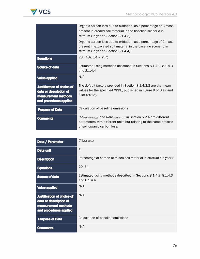
Methodology: VCS Version 4.0
76
Organic carbon loss due to oxidation, as a percentage of C mass present in eroded soil material in the baseline scenario in stratum i in year t (Section 8.1.4.3)
Organic carbon loss due to oxidation, as a percentage of C mass present in excavated soil material in the baseline scenario in stratum i in year t (Section 8.1.4.4)
Equations 28, (48), (51)- (57)
Source of data Estimated using methods described in Sections 8.1.4.2, 8.1.4.3 and 8.1.4.4
Value applied N/A
Justification of choice of data or description of measurement methods and procedures applied
The default factors provided in Section 8.1.4.3.3 are the mean values for the specified CPDE, published in Figure 9 of Blair and Aller (2012).
Purpose of Data Calculation of baseline emissions
Comments C%BSL-emitted,i,t and RateCloss-BSL,i,t in Section 5.2.4 are different parameters with different units but relating to the same process of soil organic carbon loss.
Data / Parameter C%BSL-soil,i,t
Data unit %
Description Percentage of carbon of in-situ soil material in stratum i in year t
Equations 29, 34
Source of data Estimated using methods described in Sections 8.1.4.2, 8.1.4.3 and 8.1.4.4
Value applied N/A
Justification of choice of data or description of measurement methods and procedures applied
N/A
Purpose of Data Calculation of baseline emissions
Comments N/A

Methodology: VCS Version 4.0
77
Data / Parameter Depth_iBSL,i,t
Data unit m
Description Depth of in-situ exposed soil in the baseline scenario in stratum i in year t
Equations 29
Source of data Estimated using commonly accepted procedures by the scientific community and taking note of requirements in Section 8.1.4.2
Value applied N/A
Justification of choice of data or description of measurement methods and procedures applied
See Source of data above
Purpose of Data Calculation of baseline emissions
Comments N/A
Data / Parameter Crown cover, vegetation cover
Data unit %
Description Proportion of an area covered by the herbaceous vegetation, shrubs, and/or the crowns of live trees
Equations N/A
Source of data For the baseline scenario, crown or vegetation covers must be based on a time series of vegetation composition.
Value applied N/A
Justification of choice of data or description of measurement methods and procedures applied
See Source of data above
Purpose of Data Calculation of baseline emissions
Comments Relevant for the application of the default factor in Section 8.1.4.2
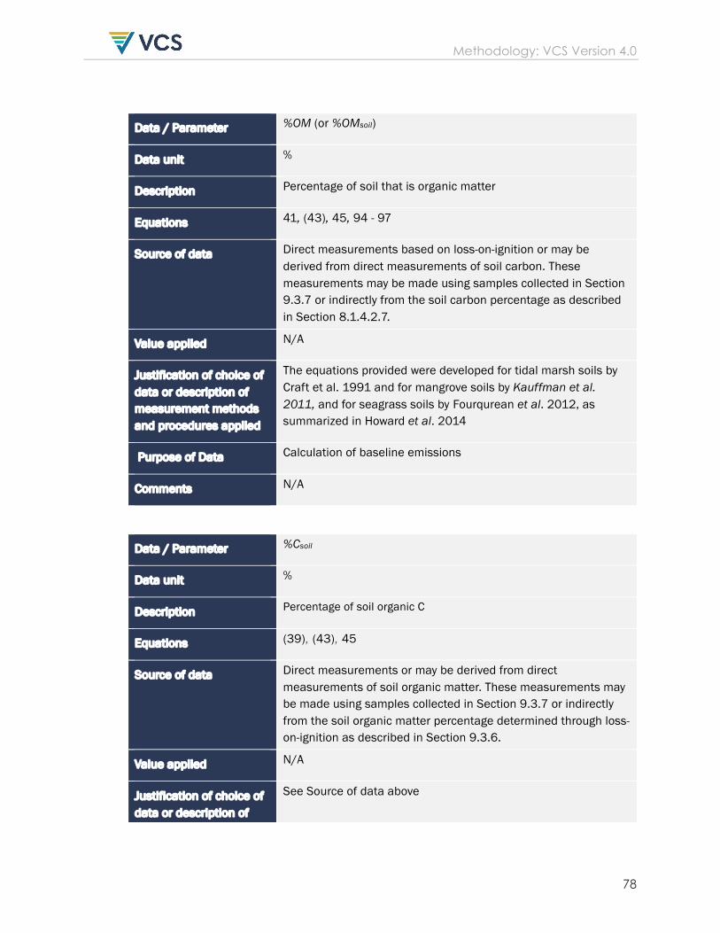
Methodology: VCS Version 4.0
78
Data / Parameter %OM (or %OMsoil)
Data unit %
Description Percentage of soil that is organic matter
Equations 41, (43), 45, 94 - 97
Source of data Direct measurements based on loss-on-ignition or may be derived from direct measurements of soil carbon. These measurements may be made using samples collected in Section 9.3.7 or indirectly from the soil carbon percentage as described in Section 8.1.4.2.7.
Value applied N/A
Justification of choice of data or description of measurement methods and procedures applied
The equations provided were developed for tidal marsh soils by Craft et al. 1991 and for mangrove soils by Kauffman et al. 2011, and for seagrass soils by Fourqurean et al. 2012, as summarized in Howard et al. 2014
Purpose of Data Calculation of baseline emissions
Comments N/A
Data / Parameter %Csoil
Data unit %
Description Percentage of soil organic C
Equations (39), (43), 45
Source of data Direct measurements or may be derived from direct measurements of soil organic matter. These measurements may be made using samples collected in Section 9.3.7 or indirectly from the soil organic matter percentage determined through loss- on-ignition as described in Section 9.3.6.
Value applied N/A
Justification of choice of data or description of
See Source of data above
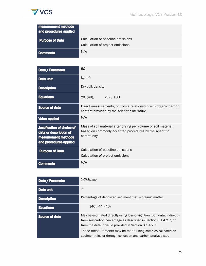
Methodology: VCS Version 4.0
79
measurement methods and procedures applied
Purpose of Data Calculation of baseline emissions
Calculation of project emissions
Comments N/A
Data / Parameter BD
Data unit kg m-3
Description Dry bulk density
Equations 29, (49), (57), 100
Source of data Direct measurements, or from a relationship with organic carbon content provided by the scientific literature.
Value applied N/A
Justification of choice of data or description of measurement methods and procedures applied
Mass of soil material after drying per volume of soil material, based on commonly accepted procedures by the scientific community.
Purpose of Data Calculation of baseline emissions
Calculation of project emissions
Comments N/A
Data / Parameter %OMdepsed
Data unit %
Description Percentage of deposited sediment that is organic matter
Equations (40), 44, (46)
Source of data May be estimated directly using loss-on-ignition (LOI) data, indirectly from soil carbon percentage as described in Section 8.1.4.2.7, or from the default value provided in Section 8.1.4.2.7.
These measurements may be made using samples collected on sediment tiles or through collection and carbon analysis (see

Methodology: VCS Version 4.0
80
Section 9.3.7) of suspended sediments in tidal channels or sediments deposits in tidal flats.
Value applied N/A
Justification of choice of data or description of measurement methods and procedures applied
LOI may be assessed using standard laboratory procedures
Purpose of Data Calculation of baseline emissions
Calculation of project emissions
Comments N/A
Data / Parameter %Cdepsed
Data unit %
Description Percentage of deposited sediment that is organic C; %
Equations 44, (46), (47)
Source of data May be estimated directly using loss-on-ignition (LOI) data or indirectly from soil carbon percentage as described in Section 8.1.4.2.7.
These measurements may be made using samples collected on sediment tiles or through collection and carbon analysis (see Section 9.3.7) of suspended sediments in tidal channels or sediments deposits in tidal flats.
Value applied N/A
Justification of choice of data or description of measurement methods and procedures applied
The default factor is derived from the maximum value (conservative) provided by Mayer 1994 Figure 4
Purpose of Data Calculation of baseline emissions
Calculation of project emissions
Comments N/A
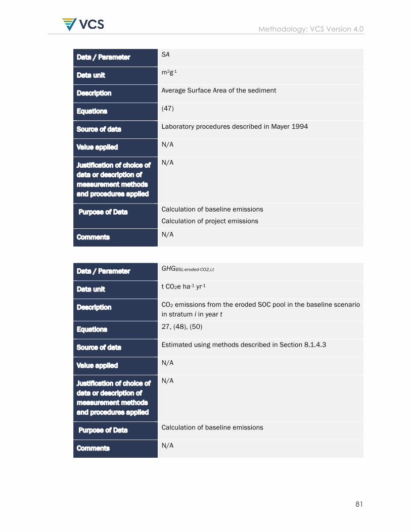
Methodology: VCS Version 4.0
81
Data / Parameter SA
Data unit m2g-1
Description Average Surface Area of the sediment
Equations (47)
Source of data Laboratory procedures described in Mayer 1994
Value applied N/A
Justification of choice of data or description of measurement methods and procedures applied
N/A
Purpose of Data Calculation of baseline emissions
Calculation of project emissions
Comments N/A
Data / Parameter GHGBSL-eroded-CO2,i,t
Data unit t CO2e ha-1 yr-1
Description CO2 emissions from the eroded SOC pool in the baseline scenario in stratum i in year t
Equations 27, (48), (50)
Source of data Estimated using methods described in Section 8.1.4.3
Value applied N/A
Justification of choice of data or description of measurement methods and procedures applied
N/A
Purpose of Data Calculation of baseline emissions
Comments N/A
Methodology: VCS Version 4.0
82
Data / Parameter CBSL-eroded,i,t
Data unit t C ha-1 yr-1
Description C mass present in eroded soil material in the baseline scenario in stratum i in year t
Equations (48), (49)
Source of data Estimated using methods described in Section 8.1.4.3
Value applied N/A
Justification of choice of data or description of measurement methods and procedures applied
N/A
Purpose of Data Calculation of baseline emissions
Comments N/A
Data / Parameter C%BSL-eroded,i,t
Data unit %
Description Percentage of carbon of soil material eroded in the baseline scenario
Equations (49)
Source of data Estimated using methods described in Section 8.1.4.3
Value applied N/A
Justification of choice of data or description of measurement methods and procedures applied
N/A
Purpose of Data Calculation of baseline emissions
Comments N/A

Methodology: VCS Version 4.0
83
Data / Parameter Depth_eBSL,i,t
Data unit m
Description Depth of the eroded area from the surface to the surface prior to erosion in the baseline scenario in stratum i in year t
Equations (49)
Source of data Estimated using methods described in Section 8.1.4.3
Value applied N/A
Justification of choice of data or description of measurement methods and procedures applied
See Source of data above
Purpose of Data Calculation of baseline emissions
Comments N/A
Data / Parameter GHGBSL-excav-CO2,i,t
Data unit t CO2e ha-1 yr-1
Description CO2 emissions from the SOC pool of tidal wetland soil exposed to an aerobic environment in the baseline scenario in stratum i in year t
Equations 27, (56),
(58)
Source of data Estimated using methods described in Section 8.1.4.4
Value applied N/A
Justification of choice of data or description of measurement methods and procedures applied
N/A
Purpose of Data Calculation of baseline emissions
Comments N/A

Methodology: VCS Version 4.0
84
Data / Parameter CBSL-excav,i,t
Data unit t C ha-1 yr-1
Description Soil organic carbon stock in tidal wetland soil exposed to an aerobic environment through excavation in the baseline scenario in stratum i in year t
Equations (56), (57)
Source of data Estimated using methods described in Section 8.1.4.4
Value applied N/A
Justification of choice of data or description of measurement methods and procedures applied
N/A
Purpose of Data Calculation of baseline emissions
Comments N/A
Data / Parameter C%BSL-excav,i,t
Data unit %
Description Percentage of carbon of soil material excavated in the baseline scenario
Equations (57)
Source of data Estimated using methods described in Section 8.1.4.4
Value applied N/A
Justification of choice of data or description of measurement methods and procedures applied
N/A
Purpose of Data Calculation of baseline emissions
Comments N/A

Methodology: VCS Version 4.0
85
Data / Parameter Depth_exBSL,i,t
Data unit m
Description Depth of piled-up soil material due to excavation in the baseline scenario in stratum i in year t
Equations (57)
Source of data Estimated using methods described in Section 8.1.4.4
Value applied N/A
Justification of choice of data or description of measurement methods and procedures applied
See Source of data above
Purpose of Data Calculation of baseline emissions
Comments N/A
Data / Parameter EFN2O,burn
Data unit g N2O / kg dry biomass
Description Emission factor for N2O emissions from vegetation burning
Equations 82
Source of data The project proponent may use factors that have been determined for grassland vegetation. A suitable EFN2O value is 0.21, from Table 2.5 of the 2006 IPCC Guidelines for National Greenhouse Inventories.
Value applied N/A
Justification of choice of data or description of measurement methods and procedures applied
Nitrous oxide emission factors for the combustion of herbaceous wetland vegetation are not currently available in scientific literature. However, these emissions are expected to be similar to those for grassland vegetation.
Purpose of Data Calculation of project emissions
Comments N/A

Methodology: VCS Version 4.0
86
Data / Parameter EFCH4,burn
Data unit g CH4 / kg dry biomass
Description Emission factor for CH4 emissions from vegetation burning
Equations 83
Source of data The project proponent may use factors that have been determined for grassland vegetation. A suitable EFCH4 value is 2.3, from Table 2.5 of the 2006 IPCC Guidelines for National Greenhouse Inventories.
Value applied N/A
Justification of choice of data or description of measurement methods and procedures applied
Methane emission factors for the combustion of herbaceous wetland vegetation are not currently available in scientific literature. However, these emissions are expected to be similar to those for grassland vegetation.
Purpose of Data Calculation of project emissions
Comments N/A
Data / Parameter allowable_uncert
Data unit %
Description Allowable uncertainty; 20% or 30% at a 90% or 95% confidence level, respectively
Equations (93)
Source of data N/A
Value applied N/A
Justification of choice of data or description of measurement methods and procedures applied
N/A
Purpose of Data Calculation of net GHG emissions reductions
Comments N/A

Methodology: VCS Version 4.0
87
Data / Parameter Vex,ty,i,t
Data unit m3
Description Volume of timber extracted from within stratum i (does not include slash left onsite) by species j and wood product class ty in year t
Equations 103
Source of data Data representing common practice in harvesting
Value applied N/A
Justification of choice of data or description of measurement methods and procedures applied
This volume does not include logging slash left onsite. The project proponent should also make sure that extracted volumes are gross volumes removed (i.e., not already discounting for estimated wood waste). Assignment of volume extracted to wood product class(es), must be substantiated on the basis of participatory rural appraisal (PRA) findings or records of timber sales. Assignment of volume extracted to species, must be substantiated on the basis of either PRA findings, harvest records, or a commercial inventory.
Purpose of Data Calculation of project emissions
Comments N/A
Data / Parameter Dj
Data unit t d.m. m-3
Description Basic wood density in t d.m. m-3 for species j
Equations 103
Source of data The source of data shall be chosen with priority from higher to lower preference as follows:
(a) National species-specific or group of species-specific (e.g., from National GHG inventory); (b) Species-specific or group of species-specific from neighboring countries with similar conditions. Sometimes (b) may be preferable to (a); (c) Global species-specific or group of species-specific (e.g., IPCC 2006 INV GLs AFOLU Chapter 4 Tables 4.13 and 4.14).

Methodology: VCS Version 4.0
88
Species-specific wood densities may not always be available, and may be difficult to apply with certainty in the typically species rich forests of the humid tropics, hence it is acceptable practice to use wood densities developed for forest types or plant families or species groups.
Value applied N/A
Justification of choice of data or description of measurement methods and procedures applied
Where using wood densities developed outside of the project country (cases (b) and (c) above under Source of data), wood densities must be validated with either limited destructive sampling or direct measurement of wood hardness (e.g., with a Pilodyn wood tester) in the field and correlating with wood density. Samples or measurements should be from 20-30 trees. For validation of mean forest type or species group wood densities, representation of species in the sample should be proportional to their occurrence in terms of basal area or volume in the project area (not abundance or stem density). Samples should provide representation across the length of the tree.
Wood samples are cut in discs and thickness and diameter measured to calculate green volume. Samples are oven dried (105o C) to a constant weight in the laboratory, and density calculated as dry weight (g) per unit green volume (cm3).
If the density of the samples/measurements (or mean density in the case of forest type or species group means) is within ±10% of the selected density values, then the selected density values may be used. Otherwise, a new density value must be developed with more extensive sampling, using the validation samples as a base.
Where new species are encountered in the course of monitoring, new wood density values must be sourced from the literature and validated, if necessary, as per requirements and procedures above.
Purpose of Data Calculation of project emissions
Comments N/A
Data / Parameter CFj
Data unit t C t-1 d.m.

Methodology: VCS Version 4.0
89
Description Carbon fraction of dry matter in t C t-1 d.m. for species j
Equations 103
Source of data Species- or family-specific values from the literature (e.g., IPCC 2006 INV GLs AFOLU Chapter 4 Table 4.3) shall be used if available, otherwise default value of 0.47 t C t-1 d.m. can be used.
Value applied N/A
Justification of choice of data or description of measurement methods and procedures applied
N/A
Purpose of Data Calculation of project emissions
Comments N/A
Data / Parameter SLFty
Data unit Dimensionless
Description Fraction of wood products that will be emitted to the atmosphere within 5 years of production by class of wood product ty
Equations 104
Source of data The source of data is the published paper of Winjum et al. 199833
Value applied Winjum et al. 1998 give the following proportions for wood products with short-term (<5 yr) uses after which they are retired and oxidized (applicable internationally):
Sawnwood 0.2 Woodbase panels 0.1 Other industrial roundwood 0.3 Paper and Paperboard 0.4
The methodology makes the assumption that all other classes of wood products, and where wood product class ty is unknown, are 100% oxidized within 5 years.
33 Winjum, J.K., Brown, S. and Schlamadinger, B. 1998. Forest harvests and wood products: sources and sinks of atmospheric carbon dioxide. Forest Science 44: 272-284
Methodology: VCS Version 4.0
90
Therefore SLF, by wood product class, is equal to:
Wood Product Class SLF
Sawnwood 0.2
Woodbase panels 0.1
Other industrial roundwood 0.3
Paper and paperboard 0.4
Other classes of wood products
1.0
Justification of choice of data or description of measurement methods and procedures applied
Parameter values to be updated if new empirically-based peer-reviewed findings become available.
Purpose of Data Calculation of project emissions
Comments N/A
Data / Parameter OFty
Data unit Dimensionless
Description OF = Fraction of wood products that will be emitted to the atmosphere between 5 and 100 years after production by class of wood product ty
Equations 104
Source of data The source of data is the published paper of Winjum et al. 199834
Value applied Winjum et al. 1998 gives annual oxidation fractions for each class of wood products split by forest region (boreal, temperate and tropical). This methodology projects these fractions over 95 years to give the additional proportion (OF value) that is oxidized between the 5th and 100th years after initial harvest:
Wood Product Class OF
Boreal Temperate Tropical
Sawnwood 0.36 0.60 0.84
34 Winjum, J.K., Brown, S. and Schlamadinger, B. 1998. Forest harvests and wood products: sources and sinks of atmospheric carbon dioxide. Forest Science 44: 272-284
Methodology: VCS Version 4.0
91
Woodbase panels 0.60 0.84 0.97
Other industrial roundwood
0.84 0.97 0.99
Paper and paperboard
0.36 0.60 0.99
Justification of choice of data or description of measurement methods and procedures applied
Parameter values to be updated if new empirically-based peer-reviewed findings become available. Every 10 years, project proponents should review research findings to identify further refinements to the emission factors that are empirically-based and peer-reviewed.
Purpose of Data Calculation of project emissions
Comments N/A
Data / Parameter BCEF
Data unit Dimensionless
Description Biomass conversion and expansion factor for conversion of commercial wood volume per unit area to total aboveground tree biomass per unit area; note that BCEF as defined here, and in most applications, is not applied on a per stem basis
Equations 104
Source of data Equations must have been derived using a wide range of measured variables (commercial wood volume per unit area and total aboveground biomass per unit area) based on datasets that comprise at least 30 trees. Equations must be based on statistically significant regressions and must have an r2 that is ≥ 0.8.
The source of data shall be chosen with priority from higher to lower preference as follows:
(a) Existing local forest type-specific; (b) National forest type-specific or eco-region-specific (e.g., from national GHG inventory); (c) Forest type-specific or eco-region-specific from neighboring countries with similar conditions. Sometimes (c) might be preferable to (b); (d) Global forest type or eco-region-specific (e.g., IPCC 2006 INV GLs AFOLU Chapter 4 Table 4.5)
Methodology: VCS Version 4.0
92
The project volume data to which the selected BCEF is applied must conform to the data the BCEF was originally derived from, in particular, it must match forest type, stand structure, minimum DBH, and cover the range of potential independent variable values (commercial volumes) likely to be encountered in the project area.
Care must be taken to ensure that the selected BCEF does not account for non-commercial species not represented in commercial volume estimates (i.e., is restricted to expanding merchantable volumes to account for only non-merchantable tree components).
Value applied N/A
Justification of choice of data or description of measurement methods and procedures applied
Alternatively, BCEF, where not directly available, can be calculated as wood density (t dry mass m-3 green volume) × BEF (Biomass Expansion Factor = ratio of aboveground biomass to biomass of the commercial volume).
If using BCEFs developed outside the project country (cases (c) and (d) above under Source of data), it is necessary to validate the applicability of BCEFs used. Validation is performed by:
1. Limited Measurements
• Select at least 20 plots in the project area covering a wide range of commercial volumes.
• Obtain tree measurements (e.g. DBH, height to a 10 cm diameter top) from which to calculate commercial volume and total biomass.
• Calculate commercial volume per unit area (e.g. using Smalian’s formula) and total biomass per unit area (using the biomass equation(s) selected for application in CP-AB) for each plot
• Calculate BCEF for each plot (biomass (t) / commercial volume (m3)
Graph the plot-level estimates of BCEF versus commercial volume along with the BCEF equation (predicted) to be validated. If the estimated BCEFs of the measured plots are distributed both above and below the predicted value the BCEF equation may be used. The BCEF equation may also be used if the measured plots have a BCEF consistently lower than that predicted. If graphing the BCEF of the measured plots indicates a systematic bias to overestimation of BCEF (>75% of the plots below the predicted value) then another BCEF equation must be selected or developed anew.

Methodology: VCS Version 4.0
93
Purpose of Data Calculation of project emissions
Comments N/A
Data / Parameter Pcomi,t
Data unit Dimensionless
Description Commercial volume as a percent of total aboveground volume in stratum i in year t
Equations 104
Source of data The source of data shall be chosen with priority from higher to lower preference as follows:
(a) Direct forest inventory of the project area, distinguishing commercially viable stocks on the basis of species and tree size, referencing local expert knowledge or a participatory rural assessment (PRA) of harvest practices and markets; (b) Forest inventory from a proxy area in the same region, representing the same forest type and age class, distinguishing commercially viable stocks on the basis of species and tree size, referencing local expert knowledge of harvest practices and markets National and forest type-specific or eco-region-specific (e.g., from National GHG inventory).
Value applied N/A
Justification of choice of data or description of measurement methods and procedures applied
N/A
Purpose of Data Calculation of project emissions
Comments N/A
Data / Parameter CH4-GWP
Data unit Dimensionless
Description Global Warming Potential of CH4
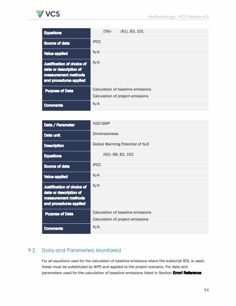
Methodology: VCS Version 4.0
94
Equations (59)– (61), 83, 101
Source of data IPCC
Value applied N/A
Justification of choice of data or description of measurement methods and procedures applied
N/A
Purpose of Data Calculation of baseline emissions
Calculation of project emissions
Comments N/A
Data / Parameter N2O-GWP
Data unit Dimensionless
Description Global Warming Potential of N2O
Equations (62)- 68, 82, 102
Source of data IPCC
Value applied N/A
Justification of choice of data or description of measurement methods and procedures applied
N/A
Purpose of Data Calculation of baseline emissions
Calculation of project emissions
Comments N/A
9.2 Data and Parameters Monitored
For all equations used for the calculation of baseline emissions where the subscript BSL is used, these must be substituted by WPS and applied to the project scenario. For data and parameters used for the calculation of baseline emissions listed in Section Error! Reference
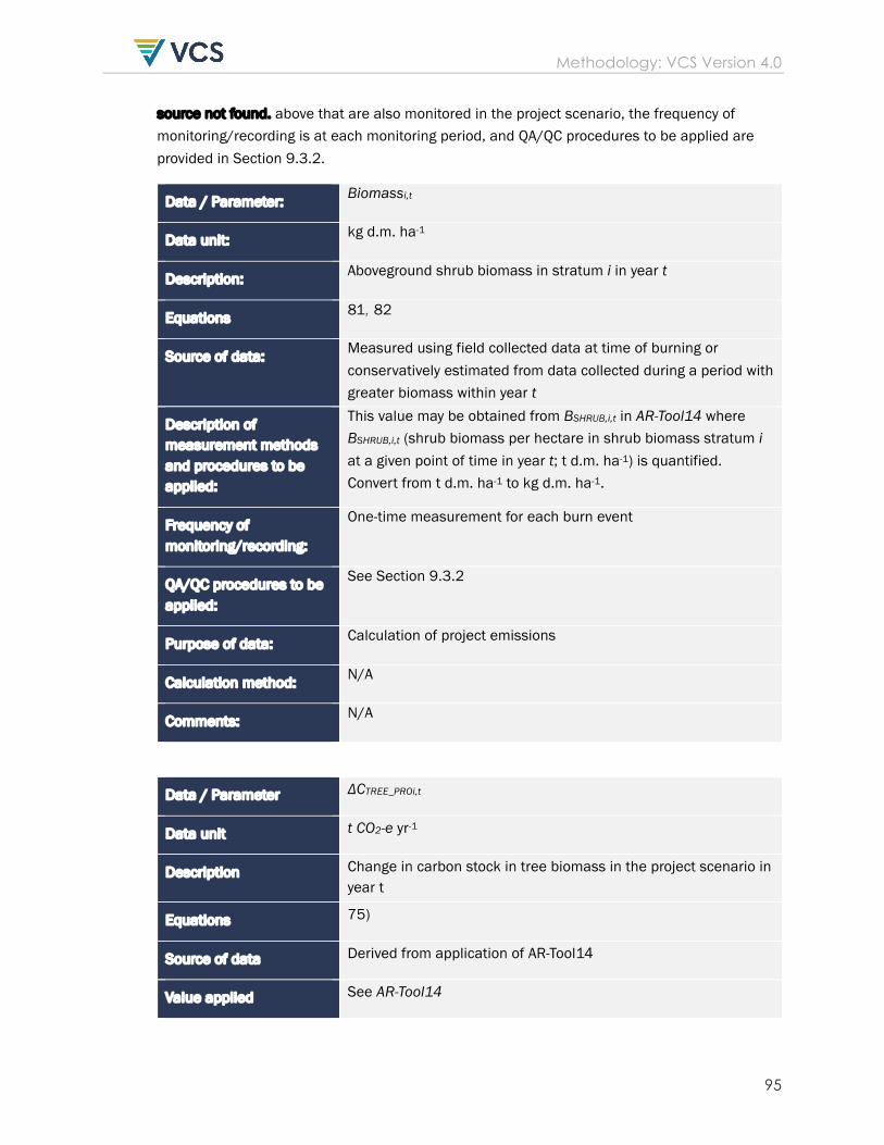
Methodology: VCS Version 4.0
95
source not found. above that are also monitored in the project scenario, the frequency of monitoring/recording is at each monitoring period, and QA/QC procedures to be applied are provided in Section 9.3.2.
Data / Parameter: Biomassi,t
Data unit: kg d.m. ha-1
Description: Aboveground shrub biomass in stratum i in year t
Equations 81, 82
Source of data: Measured using field collected data at time of burning or conservatively estimated from data collected during a period with greater biomass within year t
Description of measurement methods and procedures to be applied:
This value may be obtained from BSHRUB,i,t in AR-Tool14 where BSHRUB,i,t (shrub biomass per hectare in shrub biomass stratum i at a given point of time in year t; t d.m. ha-1) is quantified. Convert from t d.m. ha-1 to kg d.m. ha-1.
Frequency of monitoring/recording:
One-time measurement for each burn event
QA/QC procedures to be applied:
See Section 9.3.2
Purpose of data: Calculation of project emissions
Calculation method: N/A
Comments: N/A
Data / Parameter ΔCTREE_PROi,t
Data unit t CO2-e yr-1
Description Change in carbon stock in tree biomass in the project scenario in year t
Equations 75)
Source of data Derived from application of AR-Tool14
Value applied See AR-Tool14

Methodology: VCS Version 4.0
96
Justification of choice of data or description of measurement methods and procedures applied
See AR-Tool14
Purpose of Data See AR-Tool14
Comments Calculation of project emissions
Data / Parameter ΔCSHRUB_PROi,t
Data unit t CO2-e yr-1
Description Change in carbon stock in shrub biomass in the project scenario in year t
Equations 75)
Source of data Derived from application of AR-Tool14
Value applied See AR-Tool14
Justification of choice of data or description of measurement methods and procedures applied
See AR-Tool14
Purpose of Data See AR-Tool14
Comments Calculation of project emissions
Data / Parameter CWPS-herb,i,t
Data unit t C ha-1
Description Carbon stock in herbaceous vegetation in the project scenario in stratum i in year t
Equations
(78)
Source of data Direct measurements or default factor
Value applied N/A

Methodology: VCS Version 4.0
97
Justification of choice of data or description of measurement methods and procedures applied
A default factor of 3 t C ha-1 may be applied for strata with 100% herbaceous cover. For areas with a vegetation cover <100%, a 1:1 relationship between vegetation cover and CWPS,-herb,i,t must be. The default factor may be claimed for one year only during the project crediting period as herbaceous biomass quickly reaches a steady state.
Vegetation cover must be determined by commonly used techniques in field biology.
Procedures for measuring carbons stocks in herbaceous vegetation are specified in Section 9.3.6.
Purpose of Data At each monitoring period
Comments See Section 9.3.2
Data / Parameter AWPS,i (or Ai,t)
Data unit ha
Description Area of project stratum i (in year t)
Equations 4, 13, 26, (79), 82, 83
Source of data Delineation of strata must be done preferably using a Geographical Information System (GIS), which allows for integrating data from different sources (including GPS coordinates and Remote Sensing data)
Value applied See Source of data above
Justification of choice of data or description of measurement methods and procedures applied
At each monitoring period
Purpose of Data See Section 9.3.2
Comments Calculation of project emissions
Data / Parameter %OM (or %OMsoil)
Data unit %

Methodology: VCS Version 4.0
98
Description Percentage of soil that is organic matter
Equations 34, 35, (37), (39), 76, 77, (79), (79)
Source of data Direct measurements based on loss-on-ignition or may be derived from direct measurements of soil carbon. These measurements may be made using samples collected in Section 9.3.7 or indirectly from the soil carbon percentage as described in Section 8.1.4.2.7.
Value applied The equations provided were developed for tidal marsh soils by Craft et al. 1991 and for mangrove soils by Kauffman et al. 2011, and for seagrass soils by Fourqurean et al. 2012, as summarized in Howard et al. 2014
Justification of choice of data or description of measurement methods and procedures applied
At each monitoring period
Purpose of Data See Section 9.3.2
Comments Calculation of project emissions
Data / Parameter %Csoil
Data unit %
Description Percentage of soil organic C
Equations 33, (37), (39)
Source of data Direct measurements or may be derived from direct measurements of soil organic matter. These measurements may be made using samples collected in Section 9.3.7 or indirectly from the soil organic matter percentage determined through loss- on-ignition as described in Section 9.3.6.
Value applied N/A
Justification of choice of data or description of measurement methods and procedures applied
See Source of data above
Purpose of Data At each monitoring period

Methodology: VCS Version 4.0
99
Comments See Section 9.3.2
Data / Parameter Crown cover, vegetation cover
Data unit %
Description Proportion of an area covered by the herbaceous vegetation, shrubs, and/or the crowns of live trees
Equations N/A
Source of data For the project scenario, crown or vegetation cover mapping must be performed
according to established methods in scientific literature.
Value applied N/A
Justification of choice of data or description of measurement methods and procedures applied
See Source of data above
Purpose of Data At each monitoring period
Comments See Section 9.3.2
Data / Parameter: BD
Data unit: kg m-3
Description: Dry bulk density
Equations 29, (49), (57), 100
Source of data: Direct measurements, or from a relationship with organic carbon content provided by the scientific literature.
Description of measurement methods and procedures to be applied:
Mass of soil material after drying per volume of soil material, based on commonly accepted procedures by the scientific community.
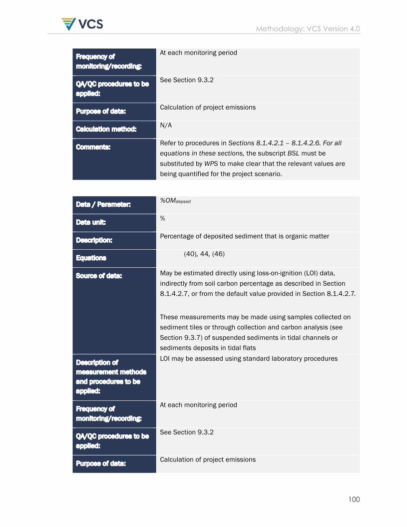
Methodology: VCS Version 4.0
100
Frequency of monitoring/recording:
At each monitoring period
QA/QC procedures to be applied:
See Section 9.3.2
Purpose of data: Calculation of project emissions
Calculation method: N/A
Comments: Refer to procedures in Sections 8.1.4.2.1 – 8.1.4.2.6. For all equations in these sections, the subscript BSL must be substituted by WPS to make clear that the relevant values are being quantified for the project scenario.
Data / Parameter: %OMdepsed
Data unit: %
Description: Percentage of deposited sediment that is organic matter
Equations (40), 44, (46)
Source of data: May be estimated directly using loss-on-ignition (LOI) data, indirectly from soil carbon percentage as described in Section 8.1.4.2.7, or from the default value provided in Section 8.1.4.2.7.
These measurements may be made using samples collected on sediment tiles or through collection and carbon analysis (see Section 9.3.7) of suspended sediments in tidal channels or sediments deposits in tidal flats
Description of measurement methods and procedures to be applied:
LOI may be assessed using standard laboratory procedures
Frequency of monitoring/recording:
At each monitoring period
QA/QC procedures to be applied:
See Section 9.3.2
Purpose of data: Calculation of project emissions

Methodology: VCS Version 4.0
101
Calculation method: N/A
Comments: Refer to procedures in Sections 8.1.4.2.1 – 8.1.4.2.6. For all equations in these sections, the subscript BSL must be substituted by WPS to make clear that the relevant values are being quantified for the project scenario.
Data / Parameter: %Cdepsed
Data unit: %
Description: Percentage of carbon in deposited sediment; %
Equations 44, (46), (47)
Source of data: May be estimated directly using loss-on-ignition (LOI) data or indirectly from soil carbon percentage as described in Section 8.1.4.2.7.
These measurements may be made using samples collected on sediment tiles or through collection and carbon analysis (see Section 9.3.7) of suspended sediments in tidal channels or sediments deposits in tidal flats.
Description of measurement methods and procedures to be applied:
The default factor is derived from the maximum value (conservative) provided by Mayer 1994 Figure 4
Frequency of monitoring/recording:
At each monitoring period
QA/QC procedures to be applied:
See Section 9.3.2
Purpose of data: Calculation of project emissions
Calculation method: N/A
Comments: Refer to procedures in Sections 8.1.4.2.1 – 8.1.4.2.6. For all equations in these sections, the subscript BSL must be substituted by WPS to make clear that the relevant values are being quantified for the project scenario.

Methodology: VCS Version 4.0
102
Data / Parameter: ETFC,y
Data unit: t CO2-e yr-1
Description: CO2 emissions from fossil fuel combustion during the year y; t CO2 yr-1
Equations
(65)
Source of data: Derived from application of CDM tool AR-Tool05 Estimation of GHG emissions related to fossil fuel combustion in A/R CDM project activities
Description of measurement methods and procedures to be applied:
See AR-Tool05
Frequency of monitoring/recording:
See AR Tool05
QA/QC procedures to be applied:
See AR Tool05
Purpose of data: Calculation of project emissions
Calculation method: See AR Tool05
Comments: Calculations are done for each stratum i
Data / Parameter: NERERROR
Data unit: %
Description: Total uncertainty for project activity
Equations 72, 73
Source of data: N/A
Description of measurement methods and procedures to be applied:
N/A
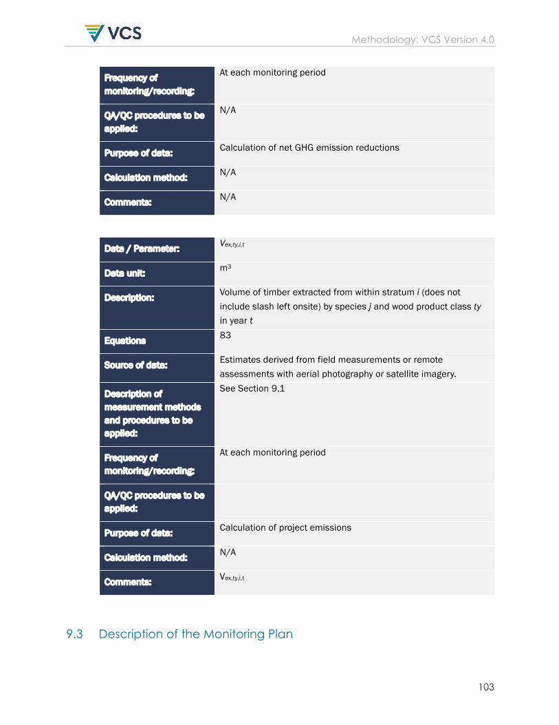
Methodology: VCS Version 4.0
103
Frequency of monitoring/recording:
At each monitoring period
QA/QC procedures to be applied:
N/A
Purpose of data: Calculation of net GHG emission reductions
Calculation method: N/A
Comments: N/A
Data / Parameter: Vex,ty,i,t
Data unit: m3
Description: Volume of timber extracted from within stratum i (does not include slash left onsite) by species j and wood product class ty in year t
Equations 83
Source of data: Estimates derived from field measurements or remote assessments with aerial photography or satellite imagery.
Description of measurement methods and procedures to be applied:
See Section 9.1
Frequency of monitoring/recording:
At each monitoring period
QA/QC procedures to be applied:
Purpose of data: Calculation of project emissions
Calculation method: N/A
Comments: Vex,ty,i,t
9.3 Description of the Monitoring Plan

Methodology: VCS Version 4.0
104
General
The main objective of project monitoring is to reliably quantify carbon stocks and GHG emissions in the project scenario during the project crediting period, prior to each verification, with the following main tasks:
• Monitor project carbon stock changes and GHG emissions • Estimate ex-post net carbon stock changes and GHG emissions, and GHG emission
reductions
The monitoring plan must contain at least the following information:
• A description of each monitoring task to be undertaken, and the technical requirements therein
• Parameters to be measured • Data to be collected and data collection techniques • Frequency of monitoring • Quality assurance and quality control (QA/QC) procedures • Data archiving procedures • Roles, responsibilities and capacity of monitoring team and management
Uncertainty and quality management
Quality management procedures are required for the management of data and information, including the assessment of uncertainty relevant to the project and baseline scenarios. As far as practical, uncertainties related to the quantification of GHG emission reductions and removals by sinks should be reduced.
To help reduce uncertainties in the accounting of emissions and removals, this methodology uses whenever possible the methods from the GPG-LULUCF, GPG-2000, the IPCC’s Revised 2006 Guidelines and peer-reviewed literature. Despite this, potential uncertainties still arise from the choice of parameters to be used. Uncertainties arising from input parameters would result in uncertainties in the estimation of both baseline net GHG emissions and project net GHG emissions, especially when global default factors are used. The project proponent must identify key parameters that would significantly influence the accuracy of estimates. Local values that are specific to the project circumstances must then be obtained for these key parameters, whenever possible. These values should be based on:
• Data from well-referenced peer-reviewed literature or other well-established published sources35;
• National inventory data or default data from IPCC literature that has, whenever possible
35 Typically, citations for sources of data used should include: the report or paper title, publisher, page numbers, publication date, etc. (or a detailed web address). If web-based reports are cited, hardcopies should be included as annexes in the project description if there is any likelihood that such reports may not be permanently available.
Methodology: VCS Version 4.0
105
and necessary, been checked for consistency against available local data specific to the project circumstances; or
• In the absence of the above sources of information, expert opinion may be used to assist with data selection. Experts will often provide a range of data, as well as a most probable value for the data. The rationale for selecting a particular data value must be described in the project description.
In choosing key parameters, or making important assumptions based on information that is not specific to the project circumstances, such as in use of default data, the project proponent must select values that will lead to an accurate estimation of net GHG emission reductions, taking into account uncertainties.
If uncertainty is significant, the project proponent must choose data such that it indisputably tends to under-estimate, rather than over-estimate, net GHG project benefits.
To ensure that carbon stocks are estimated in a way that is accurate, verifiable, transparent, and consistent across measurement periods, the project proponent must establish and document clear standard operating procedures and procedures for ensuring data quality. At a minimum, these procedures must include:
• Comprehensive documentation of all field measurements carried out in the project area. This document must be detailed enough to allow replication of sampling in the event of staff turnover between monitoring periods.
• Training procedures for all persons involved in field measurement or data analysis. The scope and date of all training must be documented.
• A protocol for assessing the accuracy of plot measurements using a check cruise and a plan for correcting the inventory if errors are discovered.
• Protocols for assessing data for outliers, transcription errors, and consistency across measurement periods.
• Data sheets must be safely archived for the life of the project. Data stored in electronic formats must be backed up.
Expert judgment
The use of expert judgment for the selection and interpretation of methods, selection of input data to fill gaps in available data, and selection of data from a range of possible values or uncertainty ranges, is well established in the IPCC 2006 good practice guidance. Obtaining well-informed judgments from domain experts regarding best estimates and uncertainties is an important aspect in various procedures throughout this methodology. The project proponent must use the guidance provided in Chapter 2 (Approaches to Data Collection), in particular, Section 2.2 and Annex 2A.1 of the IPCC 2006 good practice guidance.
Methodology: VCS Version 4.0
106
Monitoring of project implementation
Information must be provided and recorded in the project description to establish that:
1) The geographic position of the project area is recorded for all areas of wetland. The geographic coordinates of the project area (and any stratification or buffer zones inside the area are established, recorded and archived. This can be achieved by field survey (e.g., using GPS), or by using georeferenced spatial data (e.g., maps, GIS datasets, orthorectified aerial photography or georeferenced remote sensing images). The above also applies to the recording of strata.
2) Commonly accepted principles of land use inventory and management are implemented. • Standard operating procedures (SOPs) and quality control/quality assurance
(QA/QC) procedures for inventories including field data collection and data management must be applied. Use or adaptation of SOPs already applied in national land use monitoring, or available from published handbooks, or from the IPCC GPG LULUCF 2003, is recommended.
• Apply SOPs, especially, for actions likely to cause soil disturbances. • Project planning documentation, together with a record of the plan as actually
implemented during the project must be available for validation or verification, as appropriate.
Continued compliance with the applicability conditions of this methodology must be ensured by monitoring that:
• The water table is not lowered except where the project converts open water to tidal wetlands, or improves the hydrological connection to impounded waters.
• The burning of organic soil as a project activity does not occur. • Peatland fires within the project area do not occur in the project scenario. If they do
occur as non-catastrophic events, they are accounted for by cancelling the Fire Reduction Premium for the entire project or the individual project activity instance.
• N-fertilizers are not used within the project area in the project scenario.
Where the project proponent chooses to monitor alterations of water table depth in the project area to demonstrate no alteration of mean annual water table depths in adjacent areas, or that such alteration is limited to levels that do not influence GHG emissions, the project proponent must use water level gauges or vegetation assessments, or a combination of these. Water level gauges must be installed in the project area and readings must be compared with the hydrological modeling results or expert judgment on which the establishment of the project area was based. The number and spacing of water level gauges must be based on hydrological modeling or expert judgment.
Methodology: VCS Version 4.0
107
Stratification and sampling framework
Stratification of the project area into relatively homogeneous units may either increase the measuring precision without increasing the cost unduly, or reduce the cost without reducing measuring precision because of the lower variance within each homogeneous unit. The project proponent must present in the project description an ex-ante stratification of the project area or justify the lack of it. The number and boundaries of the strata defined ex ante may change during the project crediting period (ex post).
The ex-post stratification must be updated where the following occur:
• Unexpected disturbances occurring during the project crediting period (e.g., due to changes in the hydrology, fire, pests or disease outbreaks), affecting differently various parts of an originally homogeneous stratum;
• Management activities (forestry, agriculture, hydrology) that are implemented in a way that affects the existing stratification.
Established strata may be merged if the reasons for their establishment are no longer relevant.
The sampling framework, including sample size, plot size, plot shape, and determination of plot location must be specified in the project description. Where changes in carbon stocks are to be monitored (e.g., in trees), permanent sampling plots must be used, noting the following:
1) To determine the sample size and allocation among strata, the latest version of the CDM tool AR-Tool03 Calculation of the number of sample plots for measurements within A/R CDM project activities may be used. The targeted confidence interval must be 90% or 95%. Where a 90% confidence interval is adopted and the width of the confidence interval exceeds 20% of the estimated value or where a 95% confidence interval is adopted and the width of the confidence interval exceeds 30% of the estimated value, an appropriate confidence deduction must be applied, as specified in Section 8.5.2.
2) In order to avoid bias, sample plots should be marked inconspicuously.
3) The sample plot size must be established according to common practice in forest, vegetation and soil inventories.
4) To avoid subjective choice of plot locations, the permanent sample plots must be located either systematically with a random start or completely randomly inside each defined stratum. The geographical position (GPS coordinate), administrative location, stratum and stand, series number of each plot, as well as the procedure used for locating them must be recorded and archived. The sampling plots are to be as evenly distributed as possible, where larger strata have more plots than smaller strata. However, remote areas and areas with poor accessibility may be excluded for the location of sampling plots. Such areas must be mapped as separate strata and for these strata accounting of carbon stocks in tree biomass in the project scenario is conservatively omitted (see Section 5.2.2).
The choice of monitoring frequency must be justified in the project description.
Methodology: VCS Version 4.0
108
Sampling of herbaceous vegetation
Aboveground herbaceous mass (herb) is defined as a pool that includes both living plant mass (i.e., biomass) and dead plant mass (i.e., litter). All living and dead herbaceous mass is clipped above the soil surface from inside each sample frame. Dry mass is determined by either drying the entire wet sample to a constant weight, or drying a subsample of the wet mass to determine a dry-to-wet mass ratio conversion factor. Because aboveground mass can be highly seasonal, the average pool must be calculated from at least two samples representing the minimum and maximum standing stocks. Alternatively, a conservative estimate of the pool may be determined from a sample taken at the time of minimum standing stock.
Soil coring approach for estimating soil carbon
Soil organic carbon (CWPS-soil,i,t) may be estimated by determining the organic carbon accumulated above a consistent reference plane. The reference plane must be established using a marker horizon (most commonly using feldspar)36, a strongly contrasting soil layer (such as the boundary between organic and mineral soil materials), an installed reference plane (such as the shallow marker in a surface elevation table)37, a layer identified biogeochemically (such as through radionuclide, heavy metal, or biological tracers)38, a layer with soil organic carbon indistinguishable from the baseline SOC concentration (as determined in Section 8.1.4.2)39 or other accepted technologies. Note that feldspar marker horizons should not be used in systems where they are unstable, such as some sandy soils and systems with significant bioturbation. The material below the reference plane may be conservatively assumed to have zero change due to project activities.
The material located above the reference plane must be analyzed for total carbon and bulk density. Sediment samples may be collected for the estimation of %Cdepsed (see Section 8.1.4.2.7) using sediment tiles,40 through collection of suspended sediments in tidal channels during a period of high suspended sediment concentration or by collecting cores of sediment deposits in tidal flats. Total organic carbon must be analyzed directly using CHN elemental analysis or the Walkley-Black chromic acid wet oxidation method or determined from loss-on-ignition (LOI) data using the following equation:
%C = 0.04 × %OM + 0.0025 × %OM2 (only for marsh soils) 41 (95)
%C = 0.415 × %OM + 2.8857 (only for mangrove soils) 42 (96)
36 Cahoon & Turner 1989 37 Cahoon et al. 2002 38 DeLaune et al. 1978 39 Greinier et al. 2013 40 Pasternack and Brush 1998 41 Craft et al. 1993 42 Kauffman et al. 2011, Howard et al. 2014

Methodology: VCS Version 4.0
109
%C = -0.21 + 0.40 (%OM) (only for seagrass soils with %OM < 20%) 43 (97)
%C = -0.33 + 0.43 (%OM) (only for seagrass soils with %OM > 20%) 44 (98)
Alternatively, an equation developed using site-specific data may be used or an equation from peer-reviewed literature may be used if the equation represents soils from the same or similar systems as those in the project area.
Inorganic carbon should be removed from samples if present in significant quantities, usually through acid treatment (such as sulfurous or hydrochloric acid). Live coarse below-ground tree biomass should be removed from soil samples prior to analysis. Additional live below-ground biomass may be removed or included. Soil samples collected may be aggregated to reduce the variability.
The mass of carbon per unit area is calculated as follows:
𝐶!"#$%&'(',* = ∑ $𝐶𝐹#+,,%-./(0 × 𝐵𝐷 × 𝑇ℎ𝑖𝑐𝑘𝑛𝑒𝑠𝑠 × 1003120/*3'45 (99)
Where: CWPS-soil,i,t = Carbon stock in the project scenario in stratum i in year t; t C ha-1
44/12 = Ratio of molecular weight of CO2 to carbon; dimensionless Ndepth = Number for soil horizons, based on subdivisions of soil cores CFSOC_sample = Carbon fraction of the sample, as determined in laboratory; % BD = Bulk density, as determined in laboratory; g cm-3 Thickness = Thickness of soil horizon; cm 100 = Conversion factor of g cm-3 to tonne ha-1
Monitoring CH4 and N2O emissions
Direct measurement of CH4 and/or N2O emissions may be made with either a closed chamber technique or a chamber-less technique such as eddy covariance flux. For eddy covariance methods, the guidelines presented in VCS methodology VM0024 Methodology for Coastal Wetland Creation must be followed, taking into account the additional guidance below.
Flux measurements are expected to conform to standard best practices used in the scientific community45. The basic design of the closed chamber for wetlands requires a base that extends into the soil (5 cm minimum), and a chamber that is placed over the plants and sealed to the base. To prevent the measurement from disturbing CH4 emissions, the base should be placed at least one day in advance, and the plot should be approached on an elevated ramp or boardwalk when taking samples, although failure to do so is conservative because it will cause higher fluxes. CH4 flux is calculated as the difference in initial and final headspace CH4 concentration, without removing non-linear increases caused by bubble (ebullition) fluxes that
43 Fourqurean et al. 2012 as summarized in Howard et al. 2014 44 Fourqurean et al. 2012 as summarized in Howard et al. 2014 45 Oremland 1975
Methodology: VCS Version 4.0
110
may have occurred. Initial and final concentrations will be determined as the average of duplicate determinations. Because CH4 and N2O emissions can be low from tidal wetlands, it may be necessary to enclose large areas (≥ 0.25 m2) or lengthen the measurement period to improve sensitivity.
Methane emissions from strata lacking vegetation (<25% cover), such as open water, hollows or ponds, can be dominated by episodic bubble emissions (i.e., ebullition). Chambers for open water emissions are typically a single piece that floats such that the bottom extends under the water surface (5 cm minimum). Floating chambers must be deployed for a minimum of 4 days.
Eddy covariance techniques sense total CH4 and N2O emissions (diffusive and ebullition) at high temporal resolution; such systems must be deployed for a minimum of 48 hours of useable data.
CH4 and N2O emission estimates must be either accurate or conservative. Accurate estimates must account for variation in time caused by changes in plant activity, temperature, water table depth, salinity and other sources of variation, and in space caused by factors such as topography (e.g., hummocks versus hollows) or plant cover. A conservative estimate may be based on direct measurements taken at times and places in which CH4 or N2O emissions are expected to be the highest based on expert judgment, datasets or literature.
Fluxes must be measured in the stratum with the highest emissions. For CH4, these are likely to be strata in the wettest strata that support emergent vegetation, but may include stagnant pools of water. Eddy flux towers must be placed so that the footprint lies in the stratum with the highest CH4 or N2O emissions for 50% of the time. CH4 fluxes must be measured when the water table is <10 cm from the soil surface, during times of year when emissions are highest, such as the warmest month and/or wettest month. When CH4 emission rates incorporate measurements from periods of time outside the peak, they must be made at approximately monthly intervals.
In addition to the conservative principles above, the project proponent must consider other factors that are specific to the method applied. In particular, closed chambers must be transparent and deployed in daylight unless it is can be shown that CH4 emissions are not sensitive to light.
Regardless of method, emissions must be averaged and expressed as daily (24 hour) rates and converted to annual estimates using the following equations:
GHGWPS-soil-CH4,i,t = GHGCH4-daily,i,t × 365 × CH4-GWP × 100 (100)
Where: GHGWPS-soil-CH4,i,t = CH4 emissions from the SOC pool in the project scenario in stratum i in year t; t CO2e ha-1 yr-1 GHGCH4-daily,i,t = Average daily CH4 emissions in the baseline scenario based on direct measurements of stratum i in year t; mg CH4 m-2 d-1 CH4-GWP
= Global warming potential of CH4; dimensionless

Methodology: VCS Version 4.0
111
i = 1, 2, 3 …MWPS strata in the baseline scenario t = 1, 2, 3, … t* years elapsed since the project start date 100 = Conversion factor of mg m-2 to tonne ha-1
GHGWPS-soil-N2O,i,t = GHG N2O -daily,i,t × 365 × N2O-GWP × 100 (101)
Where: GHGWPS-soil-N2O,i,t = N2O emissions from the SOC pool in the project scenario in stratum i in year t; t CO2e ha-1 yr-1 GHG N2O-daily,i,t = Average daily N2O emissions in the baseline scenario based on direct measurements of stratum i in year t; mg N2O m-2 d-1 N2O-GWP
= Global warming potential of N2O; dimensionless
i = 1, 2, 3 …MWPS strata in the baseline scenario t = 1, 2, 3, … t* years elapsed since the project start date 100 = Conversion factor of mg m-2 to tonne ha-1
Where the default factor approach is used for CH4 emissions (see Section 8.1.4.5.4), the salinity average or salinity low point will be measured on shallow pore water (within 30 cm from soil surface) using a handheld salinity refractometer or other accepted technology. The salinity average must be calculated from observations that represent variation in salinity during periods of peak CH4 emissions (e.g., during the growing season in temperate ecosystems or the wet season in tropical ecosystems). When the number of observations during this period is small (fewer than one per month for one year), the salinity low point from these data must be used. The salinity of the floodwater source (e.g., an adjacent tidal creek) during this period may be used as a proxy for salinity in pore water provided there is regular hydrologic exchange between the source and the wetland (i.e., the source floods the wetland at least on 20% of high tides).
Monitoring of soil subsidence
Where soil subsidence on drained wetlands is used as a proxy for carbon loss and CO2 emissions, applied techniques and calculations must follow international standards of application or local standards as laid out in pertinent scientific literature or handbooks. The lowering of the organic soil surface over time (subsidence) must be measured relative to a fixed point (datum) (e.g., using a pole fixed in the mineral subsoil). Dipwells used for water table depth monitoring may be used for subsidence monitoring with the advantage that water table depth and subsidence are monitored at the exact same location. In areas where fire may occur, it is best (also) to place iron poles. If poles are lost due to fire, new poles must be installed. Height losses due to fire must be treated separately from those caused by microbial oxidation of the organic soil in assessing carbon losses.
Interpolation of the trend in organic soil height loss over a longer period surrounding the fire event allows for quantifying height loss due to the fire. At least 10 replicate subsidence poles must be evenly distributed per stratum. To prevent disturbance, poles may need to be fenced
Methodology: VCS Version 4.0
112
in. In order to avoid disturbance of the organic soil surface during readings it is advisable to place boardwalks. For remote and inaccessible areas, the project proponent may rely on vegetation cover as an indicator for water table depth and associated subsidence rates as supported by data or literature references in a conservative way. The minimum monitoring frequency for soil subsidence is once a year.
Consolidation of the saturated organic soil below the water table may contribute to subsidence over multiple years. The project proponent must conservatively assess the contribution of consolidation to overall subsidence by reference to literature values or expert judgment or demonstrate that consolidation plays an insignificant role in overall subsidence (< 5%).
The calculation of carbon loss rates from subsidence data must follow pertinent scientific literature (e.g., Couwenberg & Hooijer 2013) and usually requires data on the volumetric carbon content of the organic soil. When subsidence measurements are used to establish emission factors to be associated with other proxies, measurements must be carried out over a period of at least 24 months to cover intra- and inter-annual variability.
Estimation of Eroded Soil Depth and Depth of Soil Exposed to Aerobic Conditions
Soil carbon loss may occur through three mechanisms: 1) vertical edge erosion at a wetland edge or channel bank, generally occurring at the seaward margin of wetlands exposed to wave energy, 2) horizontal surface soil erosion; and/or 3) soil exposure to aerobic conditions.
1. Vertical edge erosion at a wetland edge or channel bank: The depth of eroded soil may be measured in the field directly from the difference in elevation between the emergent wetland surface at the wetland edge to the surface of an adjacent mudflat, or sediments below adjacent waters. The adjacent point must be chosen conservatively, and must represent the shallowest point of the transition from the wetland to mudflat or adjacent subaquatic sediment surface. Determination of the surface elevation of mudflat slope must be based upon the projected amount of emergent wetland retreat. Internal loss of sediment through channel enlargement and or channel network expansion occurs in wetlands with insufficient sediment supply to build at a pace matching sea level rise in settings with a tidal range greater than 1 m. Change in channel volume can be calculated using hydraulic geometry equations and approaches.46
2. Horizontal surface soil erosion: Soil depth may be calculated by direct measurement at a reference site with reference to a datum that can be justified as not having shifted vertically relative to the original soil surface. This datum may be depth to a mineral soil horizon that has not shifted due to compaction or a bedrock soil horizon, a point on mangrove stumps held in place vertically (generally due to soils composed of coarse silt
46 e.g., Allen 2000; Williams and Orr 2002

Methodology: VCS Version 4.0
113
or sand), or through radiometric analysis to identify the age of exposed soil surfaces.
3. Soil exposure to aerobic conditions: The depth of soil exposed to aerobic conditions through drainage is intended to identify the depth at which anaerobic conditions no longer suppress organic matter decomposition as they do in wetland soils. In wetland science, these anaerobic conditions are generally understood to correspond to the conditions in which iron is reduced. The depth to which the soil is reducing with respect to iron may be identified using platinum electrodes, IRIS (Indicator of Reduction in Soils) Tubes,47 the presence of reduced iron in pore water or on soil ped surfaces (indicated with Alpha-alpha-Dipyridyl or other laboratory analysis), or other accepted technologies. These methods must be used during the time of year with the peak height of anaerobic conditions (i.e., peak sustained water table and sufficient temperature for microbial activity48).
Monitoring Water Table
If water table is used as a proxy for carbon loss and GHG emissions, monitoring of water tables in the project or proxy area must be based on measurements in appropriate strata. Water table depth measurements can be continuous with data loggers and using min-max devices or simple water level gauges (dip wells consisting of e.g., perforated PVC tubes), Applied techniques must follow international standards of application or local standards as laid out in pertinent scientific literature or handbooks.
Water table depth measurements must be carried out at least every two months. At least 10 replicate dip wells must be evenly distributed per stratum, to ensure data consistency also when dip wells are lost. In peat swamp forest, dip wells must be placed in surface depressions between tree mounds. Visual inspection of the multiple records within a single stratum allows for identification of outlier values at single locations, indicating measurement errors that should be excluded from analysis. For remote and inaccessible areas, project proponents may rely on vegetation cover as an indicator for water table depth as supported by data or literature references in a conservative way.
10 REFERENCES Allen, JRL 2000. Morphodynamics of Holocene salt marshes: A review sketch from the Atlantic and southern North Sea coasts of Europe. Quaternary Science Reviews 19: 1155-1231.
47 Rabenhorst et.al. 2013
48 Vaughan et.al. 2009

Methodology: VCS Version 4.0
114
Anisfeld, S.C., M.J. Tobin, G. Benoit 1999. Sedimentation rates in flow-restricted and restored salt marshes in Long Island Sound. Estuaries 22: 231-244.
Ballhorn U, Siegert F, Mason M and S Limin 2009. Derivation of burn scar depths and estimation of carbon emissions with LIDAR in Indonesian peatlands. Proc Natl Acad Sci USA 106(50): 21213-21218.
Blair, N.E., and Aller, R.C. 2012. The Fate of Terrestrial Organic Carbon in the Marine Environment. Annual Review of Marine Science 4(1): 401–423.
Cahoon, DR, JC Lynch, BC Perez, B Segura, R Holland, C Stelly, G Stephenson, and P Hensel 2002. A device for high precision measurement of wetland sediment elevation: II. The rod surface elevation table. Journal of Sedimentary Research 72(5): 734-739.
Cahoon, DR and RE Turner 1989. Accretion and canal impacts in a rapidly subsiding wetland II. Feldspar marker horizon technique, Estuaries, 12: 260-268.
Chmura, GL, SC Anisfeld, DR Cahoon, and JC Lynch 2003. Global carbon sequestration in tidal, saline wetland soils. Global biogeochemical cycles 17: 1111-1123. doi:10.1029/2002GB001917
Couwenberg, J and Hooijer A 2013. Towards robust subsidence-based soil carbon emission factors for peat soils in south-east Asia, with special reference to oil palm plantations. Mires and Peat 12: Art. 1. (Online: http://www.mires-and-peat.net/map12/map_12_01.htm)
Craft, C.B., E.D. Seneca, and S.W. Broome. 1991. Loss on Ignition and Kjeldahl Digestion for Estimating Organic Carbon and Total Nitrogen in Estuarine Marsh Soils: Calibration with Dry Combustion. Estuaries 14(2): 175.
DeLaune, RD, WH Patrick Jr, and RJ Buresh 1978. Sedimentation rates determined by 137Cs dating in a rapidly accretion salt marsh, Nature 275: 532-533.
Duarte, CM, H Kennedy, N Marbàa, and I Hendriks 2013. Assessing the capacity of seagrass meadows for carbon burial: Current limitations and future strategies. Ocean & Coastal Management 83: 32-38.
French, J 2006. Tidal marsh sedimentation and resilience to environmental change: Exploratory modelling of tidal, sea-level and sediment supply forcing in predominantly allochthonous systems. Marine Geology 235: 119-136.
Greiner, JT, KJ McGlathery, J Gunnell, BA McKee. 2013. Seagrass restoration enhances “blue carbon” sequestration in coastal waters. PLoS ONE 8(8): e72469.
Howard, J., Hoyt, S., Isensee, K., Pidgeon, E., Telszewski, M. (eds.) (2014). Coastal Blue Carbon: Methods for assessing carbon stocks and emissions factors in mangroves, tidal salt marshes, and seagrass meadows. Conservation International, Intergovernmental Oceanographic Commission of UNESCO, International Union for Conservation of Nature. Arlington, Virginia, USA.

Methodology: VCS Version 4.0
115
IPCC 2006. IPCC Guidelines for National Greenhouse Gas Inventories, Prepared by the National Greenhouse Gas Inventories Programme, Eggleston H.S., Buendia L., Miwa K., Ngara T. and Tanabe K. (eds). Published: IGES, Japan.
Kauffman, J.B., Heider, C., Cole, T.G., Dwire, K.A., Donato, D.C. (2011). Ecosystem carbon stocks of Micronesian mangrove forests. Wetlands 31: 343–352.
Mayer, L.M. 1994. Surface area control of organic carbon accumulation in continental shelf sediments. Geochimica et Cosmochimica Acta 58(4): 1271–1284.
McGlathery, KL, LK Reynolds, LW Cole, RJ Orth, SR Marion, A Schwarzchild 2012. Recovery trajectories during state change from bare sediment to eelgrass dominance. Marine Ecology Progress Series 448: 209-221.
Mitsch, WJ, and JG Gosselink 2007. Wetlands. 4th ed. John Wiley & Sons, Inc., Hoboken, NJ.
Morris, JT, Edwards, J, Crooks, S, Reyes, E 2012. Assessment of Carbon Sequestration Potential in Coastal Wetlands. Pp 517-532. In: Recarbonization of the Bioshpere: Ecosystem and Global Carbon Cycle. R. Lal, K. Lorenz, R. Hüttl, B. U. Schneider, J. von Braun (eds). Springer.
Needelman, BA, IM Emmer, S Emmett-Mattox, S Crooks, JP Megonigal, D Myers, MPJ Oreska, and K McGlathery 2018. The science and policy of the verified carbon standard methodology for tidal wetland and seagrass restoration. Estuaries and Coasts 41(8): 2159-2171
Oremland, RS 1975. Methane Production in Shallow-Water, Tropical Marine Sediments. Applied Microbiolology 30(4): 602-608.
Orr, MK, Crooks, S and William, PB 2003. Issues in San Francisco Estuary tidal restoration: Will restored tidal marshes be sustainable? San Francisco Estuary and Watershed Science 1(1): 108-142. http://www.escholarship.org/uc/item/8hj3d20t
Poffenbarger, H, BA Needelman, and JP Megonigal 2011. Salinity influence on methane emissions from tidal marshes. Wetlands 31: 831-842.
Rabenhorst, M.C., DeLaune, R.D., Reddy, K.R., Richardson, C.J., and Megonigal, J.P. 2013. Using Synthesized Iron Oxides as an Indicator of Reduction in Soils. In: SSSA Book Series. Soil Science Society of America.
Smith, CJ, RD DeLaune, and WH Patrick Jr 1983. Nitrous oxide emission from Gulf Coast wetlands. Geochimica et Cosmochimica Acta, 47: 1805-1814.
Stralberg, S, Brennan, M, Callaway, JC, Wood, JK Schile, LM, Jongsomjit, D, Kelly, M Parker, VM, Crooks, S 2011. Evaluating tidal marsh sustainability in the face of sea-level rise: a hybrid modeling approach applied to San Francisco Bay PlosONE. http://www.plosone.org/article/info%3Adoi%2F10.1371%2Fjournal.pone.0027388
Williams, P.B. and Orr, M.K. 2002. Physical evolution of restored breached levee salt marshes in the San Francisco Bay estuary. Restor. Ecol. 10: 527-542.

Methodology: VCS Version 4.0
116
Methodology: VCS Version 4.0
117
APPENDIX 1: LONG-TERM CARBON STORAGE IN WOOD PRODUCTS Introduction
The procedures included in this appendix allow for the ex-ante estimation of carbon stocks in the long-term wood products pool in the project scenario. The procedures are applicable to all cases where wood is harvested for conversion to wood products for commercial markets, for all forest types and age classes.
The approach outlined employs an emission factor (WW) derived by Winjum et al. 1998. In the event that new research findings updating or refining (e.g., for specific countries) the WW factor become available in the future (during the project crediting period), they must be used in place of the factors included in this appendix; otherwise the factors will remain valid. The use of this appendix requires that project proponents review research findings (that produce emissions factors compatible with the conceptual framework here) at least every 10 years to identify further refinements to the emission factors that are empirically based and peer reviewed.
All factors are derived from Winjum et al. 1998.
If approved timber harvest plans, specifying harvest intensity per strata in terms of volume extracted per ha, are available for the project area, use Option 1. If approved harvest plans are not available, use Option 2.
Once actual extraction data is obtained from the project site, they must be monitored and used for calculations. At each verification event, the long-term average must be recalculated based on past harvested volumes and most recent forecasts.
Option 1: Direct Volume Extraction Estimation
Step 1: Identify the wood product class(es) (ty; defined here as sawnwood, wood-based panels, other industrial roundwood, paper and paper board, and other) that are the anticipated end use of the extracted carbon calculated in Step 2.
Step 2: Calculate the biomass carbon of the volume extracted by wood product type ty from within the project boundary:
𝐶`%,(a,+,( = ∑ (𝑉/b,(a,c,+ × 𝐷c × 𝐶𝐹c ×::);
#c$) ) (102)
Where: CXB,ty,i = Extracted biomass carbon by class of wood product ty from stratum i in year t; t CO2e Vex,ty,i,t = Volume of timber extracted from within stratum i (does not include slash left

Methodology: VCS Version 4.0
118
onsite) by species j and wood product class ty in year t; m3 Dj = Mean wood density of species j; t d.m.m-3 CFj = Carbon fraction of biomass for tree species j; t C t-1 d.m. j = 1, 2, 3, … S tree species ty = Wood product class – defined here as sawnwood (s), wood-based panels (w), other industrial roundwood (oir), paper and paper board (p), and other (o) i = 1, 2, 3 …M strata t = 1, 2, 3, … t* years elapsed since the project start date 44/12 = Ratio of molecular weight of CO2 to carbon, t CO2e t C-1
Step 3: Calculate the proportion of biomass carbon extracted that remains sequestered in long-term wood products.
𝐶!",+,( =∑ (𝐶`%,(a,+ × $1 −𝑊𝑊(a' ×$1 − 𝑆𝐿𝐹(a' × $1 − 𝑂𝐹(a'(a$3,d,2+C,.,2 (103)
Where: CWP,i,t = Extracted carbon in the wood products pool from stratum i in year t; t CO2e CXB,ty,i,t = Mean stock of extracted biomass carbon by class of wood product ty from stratum i; in year t t CO2e WWty = Wood waste. The fraction immediately emitted through mill inefficiency by class
of wood product ty; dimensionless SLFty = Fraction of wood products that will be emitted to the atmosphere within 5 years of timber harvest by class of wood product ty; dimensionless OFty = Fraction of wood products that will be emitted to the atmosphere between 5 and 100 years of timber harvest by class of wood product ty; dimensionless ty = Wood product class – defined here as sawnwood (s), wood-based panels (w), other industrial roundwood (oir), paper and paper board (p), and other (o) i = 1, 2, 3, … M strata t = 1, 2, 3, … t* years elapsed since the project start date
Option 2: Commercial Inventory Estimation
Step 1: Calculate the biomass carbon of the commercial volume extracted prior to or in the process of harvesting:
𝐶`%,+,( = 𝐶E%'()),+,( ×)
%4Je× 𝑃𝑐𝑜𝑚+,( (104)
Where: CXB,i,t = Extracted biomass carbon from stratum i in year t; t CO2e CAB_tree,i,t = Aboveground biomass carbon stock in stratum i in year t; t CO2e
BCEF = Biomass conversion and expansion factor (BCEF) for conversion of merchantable volume to total aboveground tree biomass; dimensionless Pcomi,t = Commercial volume as a percent of total aboveground volume in stratum i; dimensionless i = 1, 2, 3, … M strata

Methodology: VCS Version 4.0
119
t = 1, 2, 3, … t* years elapsed since the project start date
Step 2: Identify the wood product class(es) (ty; defined here as sawnwood, wood-based panels, other industrial roundwood, paper and paper board, and other) that are the anticipated end use of the extracted carbon calculated in Step 1.
Step 3: Same as Step 3 in Option 1 above.
Data and parameters available at validation are provided in Section 9.1.
Data and parameters monitored are provided in Section 9.2.
APPENDIX 2: ACTIVITY METHOD Introduction and approach
The positive list analysis described below was originally conducted only for the United States and, therefore, version 1.0 of VM0033 Methodology for Tidal Wetland and Seagrass Restoration limited the use of the activity method to this country; projects located in all other countries were required to apply the project method. The update to VM0007 REDD Methodology Framework to version 1.6 expanded its applicability to tidal wetland restoration and conservation activities. As part of this update, a new additionality module was created that expanded the original activity penetration analysis conducted for VM0033, version 1.0, to be applicable to be globally applicable. This analysis is described in the module VMD0052 Demonstration of Additionality of Tidal Wetland Restoration and Conservation Project Activities.
Many of the updates to VM0007 REDD Methodology Framework to expand its applicability to tidal wetland conservation and restoration, including the tool VMD0052 Demonstration of Additionality of Tidal Wetland Restoration and Conservation Project Activities, were based largely on VM0033. The updates to VM0033 in version 1.2 were to align it with some changes or additions made during the VM0007 update process.
The original positive list analysis is presented below. The full activity method analysis is provided in the module VMD0052, which must be used to demonstrate additionality in conjunction with this methodology.
Original analysis
Tidal wetland restoration activities in the United States are at a low level of penetration relative to their maximum adoption potential. Specifically, the activity penetration level of such activities is 2.74% (or lower), as demonstrated below. This level is below the 5% threshold specified in the VCS Standard. Therefore, tidal wetland restoration projects meeting the applicability conditions of this methodology and occurring within the 35 coastal states, commonwealths or territories of the United States of America are deemed additional.
Activity penetration is given as:
APy = OAy / MAPy
Where:
Methodology: VCS Version 4.0
121
APy = Activity penetration of the project activity in year y (percentage)
OAy = Observed adoption of the project activity in year y
MAPy = Maximum adoption potential of the project activity in year y
In determining the activity penetration for tidal wetlands, it is necessary to address seagrass meadows and other tidal wetlands separately due to how these ecosystems are treated in the data sources.
For tidal wetland restoration (excluding seagrass meadows) in the United States, these terms are further defined as follows:
OAy = The average annual aggregate of tidal wetlands restored from 2000 to 2013 as reported by the 28 National Estuary Programs (NEPs) and their partners to the U.S. Environmental Protection Agency (measured in acreage), and expanded to include restoration activities that occur in a U.S. estuary that is not an NEP.
MAPy = The sum of the following:
• A portion of the 1991 100-year Coastal Floodplain as determined by the Federal Emergency Management Agency (FEMA)
• Past tidal wetland losses to shallow open water in Louisiana due to coastal erosion
• Tidal wetland losses reported by the U.S. Fish and Wildlife Service (USFWS) from 1991 to 2013
For seagrass meadow restoration in the United States, these terms are defined as follows:
OAy = The percentage of seagrass meadow restoration projects compared to other estuary restoration projects funded by NOAA since 2000.
MAPy = The estimated acreage of seagrass meadow losses in the U.S.
Justification for Tidal Wetland Restoration Penetration Levels (Non-Seagrass)
The United States is a developed country where states have equal access to the nation’s resources. Factors causing degradation are substantially the same throughout the United States. Climate is not a factor in degradation of tidal wetlands, which occur across all climatic regions in the United States.
No complete national data sets exist for either tidal wetland loss or restoration in the United States. However, for both MAPy and OAy, conservative approximations can be made by examining the data from several sources.
Methodology: VCS Version 4.0
122
Time Period
The time period selected for determining the OAy is 2000 to 2013. This is an appropriate time period for the following reasons:
• The NEPs began reporting annual activities in 2000 and have been required to do so since 1993 by the Government Performance Results Act. The NEP database captures activities prior to 2000 as well as those from 2000 forward.
• The Estuary Restoration Act49 was signed into law in 2000. The Act made restoring estuaries a national priority and represents a recognition of the growing importance of estuary habitat restoration, including tidal wetlands. It provided funding authorization and appropriations for restoration projects, and created a federal interagency council to promote a coordinated Federal approach to estuary habitat restoration; forge effective partnerships among public agencies and between the public and private sectors; provide financial and technical assistance for estuary habitat restoration projects; and, develop and enhance monitoring and research capabilities. Prior to 2000, the lack of interagency coordination created sporadic and uncoordinated restoration actions.
• NOAA’s Community-based Restoration Program was created in 1999 within its Restoration Center and began funding projects that year with just $500,000 in funding50. The creation of this national center for restoration also indicates that a turning point for restoration was anticipated at that time. Since then, NOAA’s annual funding for restoration has grown to well over 10 million dollars.
• Restore America’ Estuaries (RAE) was established in 1997 as a national umbrella organization for regional non-profit organizations. These organizations identified estuary restoration as an emerging opportunity and established RAE to promote estuary restoration at the national level and to provide financial support for new restoration activities. The creation of RAE at this time reflects the need for a national voice to catalyze increased investment in estuary restoration.
Collectively these milestones represented a sea change in the restoration community that has greatly increased funding and capacity for restoration activities since the year 2000, and therefore the time period 2000 to 2013 will capture the preponderance of restoration activities.
Activity Penetration
The 28 National Estuary Programs are an appropriate means to quantify restoration activity. The National Estuary Program (NEP) was established under Section 320 of the 1987 Clean Water Act as a U.S. Environmental Protection Agency program to protect and restore the water quality and ecological integrity of estuaries of national significance. The NEP consists of 28 individual estuary programs in the United States. Each NEP has a Management Conference consisting of diverse
49 http://www.era.noaa.gov/information/act.html 50 Personal communication in 2000 with the Restoration Center Director, James Burgess.

Methodology: VCS Version 4.0
123
stakeholders including citizens, local, state and federal agencies, as well as non-profit and private sector interests. They emphasize a collaborative approach to establishing and implementing locally-based Comprehensive Conservation and Management Plans (CCMP).
The 28 estuaries with NEPs are the most advanced in conservation planning and implementation, including ecological restoration, and as such will have the greatest activity penetration levels of estuaries in the United States. They are also among the largest and most populated estuary regions in the U.S. Estuaries not included in the NEP will typically have a much lower penetration level for tidal wetland restoration.
That estuaries in NEPs face the same or similar barriers to implementation of tidal wetland restoration projects as estuaries that do not have an NEP is supported by the expert opinions supporting this document. The experts also confirm that the levels of restoration in NEPs are much greater than the levels of restoration occurring in non-NEP estuaries in the United States.
To undertake tidal wetland restoration requires significant scientific, regulatory and ecological expertise, substantial financial resources, cooperating partners, and the ability to make long-term commitments. As a participating estuary, each of the 28 NEPs receive strong federal and state financial assistance and programmatic support in these areas - support which non-NEP estuaries do not receive.
Moreover, because the NEPs are collaborative partnerships of agencies, organizations, businesses, and others, the data reported for each NEP represents a comprehensive reporting of the restoration and creation activities undertaken by the partners. This demonstrates that the 28 NEPs are an appropriate measure of the most significant observed restoration activities in the U.S.
Additional project activities occur in non-NEP estuaries. To account for these activities, a corrective factor equal to the ratio of NEP estuary land area to non-NEP estuary land area is applied. The land area of the contiguous U.S. is 2,961,266 square miles51. Coastal counties represent 17% of this area52. Therefore, coastal counties in the contiguous U.S. cover approximately 503,415 square miles of land (17% of geographic extent). The land area of the 28 NEPs is 246,338 square miles53. The ratio of land area in NEPs to total land area of coastal counties is 49% (246,338/503,415). Because the NEPs represent the most advanced and most supported estuary programs (see expert opinions below), we discount the non-NEP estimate by 50%. A correction factor of 50% therefore more than adequately captures activity in the non-NEP estuaries and the total OAy is equal to 1.5 times the OAy for NEPs.
The Environmental Protection Agency maintains an on-line database of projects reported by the 28 NEPs. Four years of data were reviewed to calculate an average rate of adoption for 2009 through
51 U.S. Census Bureau, https://www.census.gov/geo/reference/state-area.html 52 NOAA’s List of Coastal Counties for the Bureau of the Census Statistical Abstract Series, https://www.census.gov/geo/landview/lv6help/coastal_cty.pdf 53 National Estuary Program Coastal Condition Report, Chapter 2: Condition of National Estuary Program Sites - A National Snapshot, June 2007, http://water.epa.gov/type/oceb/nep/upload/2007_05_09_oceans_nepccr_pdf_nepccr_nepccr_natchap.pdf
Methodology: VCS Version 4.0
124
2012, which was then applied to the 2000 to 2014 period. This time period includes a one-time, significant infusion of federal government funding for estuary restoration in 2009. Through the American Recovery and Reinvestment Act of 2009, the National Oceanic and Atmospheric Administration received $165 million for projects, which had to be completed within 12-18 months. This one-time investment in restoration is highly unusual over the past 14 years (since the NEP data was first captured in 2000). Including this anomalous year in establishing an average adoption rate for the selected time period is a conservative approach to estimating activity penetration because it yields an average rate of restoration that is higher than the most likely rate, and applies that rate to the entire time period for determining OAy.
All United States estuaries face a common set of barriers to tidal wetland restoration including insufficient funding, lack of willing landowners and community support, and physical and ecological limitations and changes, such as sea level rise (Vigmostad et al 2005, Restore America’s Estuaries and the Estuarine Research Federation, undated). In 2000, recognizing the critical need to provide funding for estuary habitat restoration, including tidal wetlands, and help to counter the mentioned socio-economic factors, the United States Congress passed and President Clinton signed into law, the Estuary Act of 2000, which authorized $275 million over five years for restoration activities.
OAy Method of Analysis
OAy for the NEPs was determined through a systematic review of the data sets provided by the EPA for each of the NEPs. In reviewing each data set, the analysis only includes project acreage resulting from projects, which (1) are not required by any rule, regulation, law, statute, court settlement or other mandatory action and (2) meet the definition of tidal wetland restoration provided in this methodology. Where a project description included multiple habitat types (e.g., tidal wetland, shoreline, agriculture, etc.) and/or the project description included one or more activities in addition to restoration (e.g., acquisition and barrier removal), the entire project acreage was included in the calculation. This is conservative because it will lead to a higher activity penetration. The NEP OAy calculation is provided in Table 4.
Methodology: VCS Version 4.0
125
Table 4: Calculation of OAy for the NEPs
Once the NEP OAy was determined, to ensure capture of non-NEP activities, it is increased by 50% for the Activity Penetration calculation.
OAy = NEP OAy × 1.5 = 97,422.17 acres * 1.5 = 146,133 acres
Maximum Adoption Potential
To determine MAPy, an estimate of the available area for tidal wetland restoration needs to be established. The starting point for this estimate is the “Projected Impact of Relative Sea Level Rise on the National Flood Insurance Program” prepared by the Federal Emergency Management Agency (FEMA 1991). FEMA calculated the area of coastal floodplain that would flood under a 100-year coastal flood
Estuary Program 2009 2010 2011 2012 4 year average
Peconic Bay Estuary Program - - - - - Piscataqua Region Estuaries Partnership - - 12.00 0.05 3.01 Buzzards Bay National Estuary Program 3.74 - - - 0.94 Tillamook Estuaries Partnership 46.00 44.00 16.00 4.40 27.60 Mobile Bay National Estuary Program 137.00 - 6.50 2.00 36.38 Santa Monica Bay Restoration Commission - 21.00 - - 5.25 Tampa Bay Estuary Program 142.70 61.28 - 44.54 62.13 Delaware Center for the Inland Bays 26.00 4.00 - - 7.50 Lower Columbia River Estuary Partnership - - 184.00 58.00 60.50 Indian River Lagoon National Estuary Program 1,395.75 21.26 419.00 140.30 494.08 Maryland Coastal Bays Program 64.43 1.80 104.00 189.00 89.81 Galveston Bay Estuary Program 158.00 46.81 407.06 9.00 155.22 New York-New Jersey Harbor Estuary Program 11.00 34.00 65.80 50.00 40.20 Chesapeake Bay Program 622.00 1,005.00 3,775.00 n/a 1,800.67 Puget Sound Partnership 1,277.00 140.00 505.40 101.00 505.85 Charlotte Harbor National Estuary Program 600.50 496.00 795.00 140.00 507.88 San Francisco Estuary Partnership 1,469.00 401.00 3,250.00 983.36 1,525.84 Barataria-Terrebonne Estuary Program 673.58 n/a 35.00 182.00 296.86 Sarasota Bay Estuary Program 516.00 - 30.00 5.00 137.75 Long Island Sound Study 58.65 88.00 42.56 137.70 81.73 Partnership for the Delaware Estuary 1.30 6.50 - - 1.95 Albemarle-Pamlico National Estuary Program 1.10 4.00 84.20 0.31 22.40 Barnegat Bay Partnership - - - - - Narragansett Bay Estuary Program 63.00 58.00 - - 30.25 Massachusetts Bays Program 1,442.00 133.00 54.00 21.00 412.50 Casco Bay Estuary Partnership - - - 21.80 5.45 Coastal Bend Bays and Estuaries Program 1,597.00 568.00 351.00 72.00 647.00 Morro Bay National Estuary Program n/a n/a n/a n/a n/aOne year average, 2009-2012 6,958.73 2000 to 2013 total estimate = 14*One year average 97,422.17
Sources:
Tidal Wetland Acres Restored
1. All 2009 data are from “NEP Project Information and Maps 2000-2009,” http://gispub2.epa.gov/NEPMap/archivetree/archivetree.html. (U.S. Environmental Protection Agency). From each table, only tidal wetland restoration and creation projects are counted.
2. All 2010, 2011 and 2012 data are from the “NEP Projects Table Tool,” http://gispub2.epa.gov/NEPmap/NEPTable_allyears/index.html. (National Estuary Program). From each table, only tidal wetland restoration and creation projects are counted.

Methodology: VCS Version 4.0
126
event for 1990 to be 19,500 mi2 (12,800,000 acres). A 100-year flood event is defined as a flood that statistically has a 1% chance of occurring in any given year. By definition, the coastal floodplain does not include either upland areas or existing wetland areas (wetland areas do not flood because they are already regularly inundated). The coastal floodplain consists substantially of former wetland areas that were drained and/or filled and converted to other land uses, such as agricultural, commercial, or residential uses. This area includes many but not all former tidal wetland areas that were diked or drained for agriculture and other uses (some former wetland areas are no longer in the floodplain as they are now well protected by dikes or levees, e.g., and therefore are not included in this estimate, which is conservative). Not all of the coastal floodplain area identified by FEMA is restorable or suitable for wetland creation. But for establishing an estimate of MAPy, 33% of this area (4,224,000 acres) is used as a conservative (low) estimate.
The FEMA estimate was made in 1991 and only includes land areas subject to flooding. Therefore, we also include in the MAPy tidal wetland losses since 1991 and tidal wetlands that have drowned or converted to open water in coastal Louisiana. Virtually all of these areas are suitable for tidal wetland restoration.
Louisiana wetland losses from 1900 to 1978 are reported to be 901,200 acres (U.S. Department of the Interior 1994). The MAPy estimate does not include Louisiana coastal wetland losses between 1978 and 1986, and it is conservative to exclude that area from the MAPy.
Tidal wetland losses from 1986 to 1997 were reported to be 8,450 acres (Dahl 2000). The 1991 to 1997 portion of these losses is assumed to be 4,225 acres, a pro-rated portion of the total.
Tidal wetland losses from 1998 to 2004 were reported to be 32,400 acres (Dahl 2006).
Tidal wetland losses from 2004 to 2009 were reported to be 124,290 acres (Dahl 2011).
No data exists for 2010 to 2013 (four years). We apply the average rate of loss from the previous five year period, 2004 to 2009, which is 124,290 acres /6 years = 20,715 acres /year.
Table 5: Calculation of Maximum Adoption Potential for tidal wetland restoration (non-seagrass)
Activity Penetration Calculation for Tidal Wetlands (non-seagrass)
Maximum Adoption Potential Acres
33% of FEMA 1991 Floodplain Estimate 4,244,000 Louisiana Delta Wetland Losses 901,200 Tidal Wetland Losses 1991 to 1997 4,228 Tidal Wetland Losses 1998 to 2004 32,400 Tidal Wetland Losses 2004 to 2009 124,290 Tidal Wetland Losses 2010 to 2013 82,860
Total MAPy (non-seagrass) 5,388,978
Methodology: VCS Version 4.0
127
APy = OAy / MAPy
APy = 146,133 acres / 5, 338,978 acres
APy = 2.71%
Justification for Seagrass Meadow Restoration Penetration Levels
OAy Method of Analysis
Seagrass meadow restoration also occurs at a very low level relative to its maximum adoption level in the U.S. Evidence of this is provided by the National Oceanic and Atmospheric Administration, which maintains a Restoration Atlas (NOAA 2014). NOAA is the lead federal agency mandated with coastal and marine fisheries habitat restoration and protection, including seagrass meadow habitat. NOAA’s level of funding for seagrass meadow restoration is therefore a sufficient estimate of the total level of seagrass restoration.
The NOAA database contains information on about 2,701 habitat projects that have occurred since 2000, and only 120, or 4%, are seagrass meadow projects. The database includes numerous habitats (e.g., dune, in-stream, kelp, mangrove, oyster reef) as well as numerous activities in wetland habitats (restoration, invasive species removal, marine debris removal). Only a portion of the 120 seagrass meadow projects would meet the applicability conditions of this methodology. Therefore, including all of identified seagrass meadow restoration projects is conservative. The total acreage of estuary habitat restoration projects in the NOAA database is 49,837 acres. Seagrass meadow projects are typically conducted at a smaller scale than other habitat activities; therefore assuming that 4% of the total acreage can be attributed to seagrass restoration is conservative. The OAy for seagrass restoration is therefore 4% of 49,837 = 1,993 acres.
Maximum Adoption Potential Method of Analysis for Seagrass Restoration
Waycott et al (2009) demonstrated that seagrass meadow habitat losses in the U.S. were 853,845 acres between 1937 and 2006. The primary causes of the loss of seagrass meadows – sediment deposition, declining water quality, scarring from vessels, and disease – are typically reversible. Therefore, all of the area documented as lost is restorable. MAPy for seagrass meadow restoration is therefore 853,845 acres.
Activity Penetration Calculation for Seagrass Restoration
APy = OAy / MAPy
APy = 1,993 / 853,845 = 0.2%.

Methodology: VCS Version 4.0
128
References Dahl, T.E. 2000. Status and trends of wetlands in the conterminous United States 1986 to 1997. U.S.
Department of the Interior, Fish and Wildlife Service, Washington, D.C
Dahl, T.E. 2006. Status and trends of wetlands in the conterminous United States 1998 to 2004. U.S. Department of the Interior; Fish and Wildlife Service, Washington, D.C.
Dahl, T.E. 2011. Status and trends of wetlands in the conterminous United States 2004 to 2009. U.S. Department of the Interior; Fish and Wildlife Service, Washington, D.C.
FEMA 1991. Projected Impact of Relative Sea Level Rise on the National Flood Insurance Program.
Federal Emergency Management Agency, Federal Insurance Administration.
National Oceanic and Atmospheric Administration. Restoration Atlas. https://restoration.atlas.noaa.gov/src/html/index.html.
Restore America’s Estuaries and the Estuarine Research Federation. Undated. Principles of Estuarine Habitat Restoration. Arlington, VA.
U.S. Department of the Interior. 1994. The Impact of Federal Programs on Wetlands, Volume II: The Everglades, Coastal Louisiana, Galveston Bay, Puerto Rico, California's Central Valley, Western Riparian Areas, Southeastern and Western Alaska, The Delmarva Peninsula, North Carolina, Northeastern New Jersey, Michigan, and Nebraska. A report to Congress by the Secretary of the Interior. http://www.doi.gov/pmb/oepc/wetlands2/v2ch8.cfm
U.S. Environmental Protection Agency. NEP Project Information and Maps 2000-2009. http://gispub2.epa.gov/NEPMap/archivetree/archivetree.html.
U.S. Environmental Protection Agency. NEP Projects Table Tool. http://gispub2.epa.gov/NEPmap/NEPTable_allyears/index.html.
Vigmostad, Karen E., Nicole Mays, Allen Hance, and Allegra Cangelosi. 2005. Large-scale ecosystem restoration: Lessons for existing and emerging initiatives. Washington, DC: Northeast-Midwest Institute.
Waycott, M, C Duarte, T Carruthers, R Orth, W Dennison, S Olyarnik, A Colladine, J Fourqurean, K Heck, A Hughes, G Kendrick, W Kenworthy, F Short, and S Williams 2009. Accelerating loss of seagrasses across the globe threatens coastal ecosystems. PNAS 106(30): 12377-12381. http://www.pnas.org/content/106/30/12377.full.pdf+html
Methodology: VCS Version 4.0
129
Expert Credentials Debbie DeVore is the Gulf Restoration Program Coordinator for the US Fish & Wildlife Service, where she coordinates restoration activities for the Service offices and programs along the Gulf Coast. She has more than 15 years of experience in coastal resource management and has received numerous awards in her career.
Curtis D. Tanner is Acting Manager for the Division of Environmental Assessment and Restoration (EAR) in the U.S. Fish and Wildlife Service, where he manages staff and activities in the Watershed Protection and Restoration Branch. He provided leadership for the Puget Sound Nearshore Ecosystem Restoration Project, and has more than twenty years of experience in coastal resource management and restoration.
EXPERT OPINION I
Debbie L. DeVore Gulf Coast Restoration Program Manager U.S. Fish & Wildlife Service
Question 1 – To what extent do estuaries without a National Estuary Program face the same barriers to tidal wetland restoration activities as estuaries, which are part of a National Estuary Program? We have identified the following barriers, among others: funding, land ownership/control, political will, a local environment, which encourages partnerships, and social acceptability. Please note that we only need to consider barriers to tidal wetland restoration where it has already been identified as possible in the landscape. Based on your experience and expert judgment, do estuaries in NEPs face the same or similar barriers to implementation of tidal wetland restoration projects as estuaries that do not have an NEP? Please explain.
Answer:
While there are, no doubt, advantages afforded an estuary which has an established National Estuary Program (NEP) this does not preclude or exempt projects in these geographies from many of the same hurdles that projects face in an estuary outside the geographic of an NEP.
For example, funding is commonly the largest limiting factor in bringing a tidal restoration project to implementation, regardless of the project's location. Projects with involvement from an NEP must apply for the same limited funding as any other project (raising the same amount of match, etc.) and be held to the same reporting and fiduciary responsibilities as well. NEP supported projects must also go through the same scrutiny to obtain regulatory permission to conduct work, just as a non-NEP project does.

Methodology: VCS Version 4.0
130
Both political will and public support for projects are also similar issues faced by projects both within an NEP and outside a NEP geography. In fact, projects with NEP support or in a NEP geography may even sometimes have a bigger stigma as the public may not have a high level of trust for governmental organizations and be much less supportive of their actions. As well, working with landowners (particularly private landowners) may prove more difficult for projects with an governmental agency connection.
Tidal restoration projects and activities, while often a high priority based upon the result of natural resource partners coming together for a common restoration objective, are not necessarily given special preference towards implementation simply because they are facilitated by such a collaboration. These projects are held to the same standards (and hence work through the same barriers and hurdles) as projects in a non-NEP geography.
Question 2 – How likely is it that the rates of restoration in National Estuary Programs are greater than the rates of restoration occurring in non-NEP estuaries in the U.S.? It is our assumption that NEPs will have an overall higher rate of restoration than other estuaries because NEPs benefit from a shared state and federal commitment to estuary health, which may be absent in other estuaries. Moreover, because of the status of being an NEP, they are more likely to receive scarce federal and state resources, as well as funding from other partners. NEPs are multi-stakeholder collaborative efforts that are not found in other estuaries in the U.S. Based on your experience and expert judgment, are NEPs substantially likely to have a higher rate of restoration than non-NEP estuaries? Please explain.
Answer:
Although I may paint a picture of hard times for NEPs above - having to jump through the same regulatory hoops as other projects - that is part of doing business in coastal restoration. NEPs and their restoration partners understand this and support that we should be held to the same regulatory and accountability standards as projects in non-NEP geographies or with no connection to the Program itself. NEPs and their partners do, however, recognize the tremendous benefit to a voluntary, collaborative and strategic approach to tidal restoration (as well as other coastal conservation issues NEPs address). Many funding agencies give credit to project proponents who work as a collective multi-stakeholder partnership. There is an assumption that such a partnership represents an agreed upon set of goals, objectives, implementation procedures and monitoring for a given project. This gives a funding agency a certain level of confidence that the project will be successful and supported at a local level. Project proposals written by NEP partners are also often more well defined and in concert with requested information outlined in a funding opportunity.
To answer your question specifically, yes, I do think NEPs have a higher likelihood of receiving funds for coastal restoration. I say this for a few reasons. In today's world of limited federal and state budgets and fewer dollars to put "on-the-ground" for projects, the conservation community has been pushed to become much more strategic in our thinking. By this I mean that we are looking at how projects fit into the larger watershed or landscape, we strive to accomplish as many partners' goal and objectives as possible, and we must leverage our funds as much as we possibly can. The NEP structure, their

Methodology: VCS Version 4.0
131
associated advisory committees and public outreach capabilities, lends itself to a role in facilitating such a strategic approach.
I worked for the FWS Coastal Program nearly 10 years and can say that for many of the reasons I described above, our Program encourages and actively engages in partnership with our local NEPs. In my tenure with the Coastal Program I have worked with NEPs in both Texas and Florida. When possible, our Program staff serve on technical advisory committees, participate in strategic planning and assist in project implementation. In fact, I was involved in drafting the current Strategic Plan for our southwest Florida focal area where I identified working with the NEPs as a priority for our Program. When appropriate and feasible, the Coastal Program has and continues to invest funding towards projects such as tidal restoration activities.
Original request to expert:
On Wed, Oct 23, 2013 at 4:57 PM, Steve Emmett-Mattox wrote:
Dear Ms. Devore,
Restore America’s Estuaries is seeking to demonstrate the “additionality” of tidal wetland restoration in the U.S. for the purposes of generating carbon offsets under the Verified Carbon Standard. The VCS revised its rules in 2012 to include a standardized approach to demonstrate additionality. In order to comply with this approach, RAE has assembled a substantial data set and analysis. The data, analysis and discussion are attached. In a recent review by the VCS, they raised two questions that we would like your help in answering. I believe you to be an expert in tidal wetland restoration programs and activities in the U.S., and now seek your opinion on the following:
1 – to what extent do estuaries without a National Estuary Program face the same barriers to tidal wetland restoration activities as estuaries, which are part of a National Estuary Program? We have identified the following barriers, among others: funding, land ownership/control, political will, a local environment, which encourages partnerships, and social acceptability. Please note that we only need to consider barriers to tidal wetland restoration where it has already been identified as possible in the landscape. Based on your experience and expert judgment, do estuaries in NEPs face the same or similar barriers to implementation of tidal wetland restoration projects as estuaries that do not have an NEP? Please explain.
2 – how likely is it that the rates of restoration in National Estuary Programs are greater than the rates of restoration occurring in non-NEP estuaries in the U.S.? It is our assumption that NEPs will have an overall higher rate of restoration than other estuaries because NEPs benefit from a shared state and federal commitment to estuary health, which may be absent in other estuaries. Moreover, because of the status of being an NEP, they are more likely to receive scarce federal and state resources, as well as funding from other partners. NEPs are multi-stakeholder collaborative efforts that are not found in other estuaries in the U.S. Based on your experience and expert judgment, are NEPs substantially likely to have a higher rate of restoration than non-NEP estuaries? Please explain.
And last, please provide an up to date resume/CV, which we will share with the VCS.

Methodology: VCS Version 4.0
132
Please let me know if you have any questions about this request, and thank you for your timely response.
Cheers, Steve Emmett-Mattox Senior Director for Strategic Planning and Programs Restore America's Estuaries
EXPERT OPINION II
Curtis Tanner Acting Manager, Environmental Restoration and Assessment Division U.S. Fish and Wildlife Service 18 November 2013
Steve Emmet-Mattox Senior Director for Strategic Planning and Programs Restore America’s Estuaries Dear Steve:
I am writing in response to your September 23, 2013, email requesting my expert opinion regarding tidal wetland restoration and greenhouse gas offsets. As you know, I have over twenty years of experience working on coastal wetland restoration and protection for the U.S. Fish and Wildlife Service. The views expressed in this letter are based on my own experience and perspective, and do not reflect an official agency position. I have attached a copy of my current resume for your use in assessing my credentials.
As I understand it, you are working to establish the viability of tidal wetland restoration as a tool for use in sequestering carbon dioxide to mitigate anthropogenic greenhouse gas emissions. You seek to establish the fact that at a National scale, tidal wetland restoration in the United States is limited in spatial scale and impact. Specifically, “activity penetration”, or the prevalence of restoration project implementation relative to the opportunity for tidal wetland restoration, is relatively small. In your assessment of tidal restoration in the U.S., you estimate the “…Activity Penetration is 1.06%, which is less than 5%, and therefore tidal wetland restoration in the U.S. is additional…” as defined by the Verified Carbon Standard. In short, you assert that given the relatively small amount of tidal wetland restoration in the U.S. (as compared to opportunity and demonstrated need), investment in restoration would provide a viable alternative for carbon offset funds. I concur with your assessment.
Your analysis relied upon the most comprehensive data set available at the National level for tidal wetland restoration, accomplishment reporting from the National Estuary Program (NEP). You have specifically requested that I provide an assessment based on my experience and expert judgment whether use of these data are appropriate. First, you have asked whether estuaries covered by the NEP provide a representative sample, facing the same or similar barriers to tidal wetland restoration project
Methodology: VCS Version 4.0
133
implementation. Based on 20+ years of experience working on coastal restoration and protection issues and projects, it is my opinion that tidal wetland restoration is typically limited by a set of barriers common to estuaries throughout the United States; funding, land owner willingness, and social acceptability are nearly universal challenges for all projects and estuaries. Taken together as a whole, the geographic distribution of NEP sites provides a broad cross section of National estuarine ecosystem conditions, encompassing a range of ecological threats, fish and wildlife resource assets, and socio/political contexts. This representative diversity applies to both human and non-human aspects of coastal ecosystems.
Second, you post the question as to whether the rate of restoration derived from analysis of NEP estuaries is representative. As I understand your analysis, if NEP estuaries had a substantially lower rate of restoration than non-NEP estuaries, your activity penetration estimate of 1.06%, as compared the VCS threshold of 5%, could be challenged. Based on my experience derived from project implementation and program management, NEP estuaries likely deliver a higher rate of restoration as compared to non-NEP estuaries, if significant differences do in fact exist. I base this assertion on observations of the opportunity space provided for restoration that NEP designation provides coastal ecosystems. The Clean Water Act directs each NEP to develop and implement a Comprehensive Conservation and Management Plan (CCMP). Agencies including the U.S. Fish and Wildlife Service respond to policies and Congressional funding directives to focus restoration efforts in NEP systems, often in response to the CCMP. NEP designation also works to focus the work of state agency, tribal government, and non-governmental organization partners to address restoration needs defined by the CCMP. In Puget Sound, development and implementation of the CCMP is the role of the Puget Sound Partnership (PSP), a Washington State cabinet-level agency. PSP has led development of the current CCMP for Puget Sound, referenced as the “Action Agenda”. PSP’s Action Agenda includes specific targets for estuarine restoration required to recover the health of Puget Sound. Other non-NEP coastal ecosystems in Washington State lack this political focus and dedicated state and National funding for tidal wetland restoration.
In summary, while I have not provided a detailed review of your data sources and analysis, I am familiar with the approach you have applied in your analysis. NEP estuaries provide applicable data set for your assessment of activity penetration for restoration. CCMP’s for NEP estuaries provide a numeric objective for restoration and thus a quantifiable estimate of opportunity and need. Accomplishment reporting required by U.S. EPA delivers an accounting of acres restored which can be compared to numeric targets. The 28 NEP systems distributed throughout the United States provide a representative cross section of coastal ecosystems and the challenges and opportunities faced by restoration projects proponents. NEP designation leads to a regional focus of efforts, that delivers activity penetration rates likely equal or greater than that of non-NEP systems.
Thank-you for the opportunity to provide my perspective on your assessment. Please contact me directly if you have questions or if I can be of additional assistance.
Sincerely, Curtis D. Tanner Original request to expert:

Methodology: VCS Version 4.0
134
From: Steve Emmett-Mattox Sent: Monday, September 23, 2013 1:42 PM To: 'Tanner, Curtis' Subject: expert guidance sought, Restore America's Estuaries tidal wetland restoration and ghg offsets
Dear Mr. Tanner,
Restore America’s Estuaries is seeking to demonstrate the “additionality” of tidal wetland restoration in the U.S. for the purposes of generating carbon offsets under the Verified Carbon Standard. The VCS revised its rules in 2012 to include a standardized approach to demonstrate additionality. In order to comply with this approach, RAE has assembled a substantial data set and analysis. The data, analysis and discussion are attached. In a recent review by the VCS, they raised two questions that we would like your help in answering. I believe you to be an expert in tidal wetland restoration activities in the U.S., and now seek your opinion on the following:
1 – to what extent do estuaries without a National Estuary Program face the same barriers to tidal wetland restoration activities as estuaries, which are part of a National Estuary Program? We have identified the following barriers, among others: funding, land ownership/control, political will, a local environment, which encourages partnerships, and social acceptability. Please note that we only need to consider barriers to tidal wetland restoration where it has already been identified as possible in the landscape. Based on your experience and expert judgment, do estuaries in NEPs face the same or similar barriers to implementation of tidal wetland restoration projects as estuaries that do not have an NEP? Please explain.
2 – how likely is it that the rates of restoration in National Estuary Programs are greater than the rates of restoration occurring in non-NEP estuaries in the U.S.? It is our assumption that NEPs will have an overall higher rate of restoration than other estuaries because NEPs indicate a shared state and federal commitment to estuary health, which may be absent in other estuaries. Moreover, because of the status of being an NEP, they are more likely to receive scarce federal and state resources, as well as funding from other partners. NEPs are multi-stakeholder collaborative efforts that are not found in other estuaries in the U.S. Based on your experience and expert judgment, are NEPs substantially likely to have a higher rate of restoration than non-NEP estuaries? Please explain.
And last, please provide an up to date resume/CV, which we will share with the VCS.
Please let me know if you have any questions about this request, and thank you for your timely response.
Cheers, Steve Emmett-Mattox Senior Director for Strategic Planning and Programs Restore America's Estuaries

Methodology: VCS Version 4.0
135
DOCUMENT HISTORY Version Date Comment
1.0 20 Nov 2015 New methodology (initial version)
2.0 30 Sep 2021 Updates based on the revision to VM0007 REDD Methodology Framework, v1.6 and inclusion of that have been scrutinized under the rules for expert judgment to estimate net GHG emissions from soil in the baseline scenario.