volatility of world rice prices, import tariffs and poverty
TRANSCRIPT

Munich Personal RePEc Archive
Volatility of world rice prices, import
tariffs and poverty in Indonesia: a
CGE-microsimulation analysis
Teguh, Dartanto
Institute for Economic and Social Research, Department of
Economics, University of Indonesia, GSID, Nagoya University
December 2010
Online at https://mpra.ub.uni-muenchen.de/31451/
MPRA Paper No. 31451, posted 12 Jun 2011 00:56 UTC
Economics and Finance Indonesia, Vol. 52, No.3, pp.335-364
1
Volatility of World Rice Prices, Import Tariffs and Poverty in Indonesia:
A CGE-Microsimulation Analysis
Teguh Dartanto
PhD Student, Graduate School of International Development, Nagoya University, Japan
and
Researcher, LPEM FEUI, Department of Economics, University of Indonesia
Email Address: [email protected] or [email protected]
Abstract
This study aims at measuring the impact of world price volatility and import tariffs on rice on poverty in
Indonesia. Applying a Computable General Equilibrium-Microsimulation approach and the endogenous
poverty line, this study found that the volatility of world rice prices during 2007 to 2010 had a large effect
on the poverty incidence in Indonesia. The simulation result showed that a 60 per cent increase in world rice
price raises the head count index by 0.81 per cent which is equivalent to an increase in the number of poor
by 1,687,270. However, both the 40 per cent decrease in the effective import tariffs on rice enacted by
regulation No.93/PMK.011/2007 and the zero import tariffs implemented by regulation No.
241/PMK.011/2010 in response to high world rice prices could not perfectly absorb the negative impact
of increasing world rice prices on poverty. The 40 per cent decrease in the effective import tariffs on rice
reduced the head count index by 0.08 per cent equal to 161,546 people while the zero import tariffs on rice
reduced the head count index by 0.19 per cent equal to 390,160 people. These policies might not be enough
to absorb the negative impact of an increase in world rice prices from 2007-2010, because, during this period,
the world rice prices increased on average by almost 71 per cent, which have impoverished approximately two
million people. Moreover, protection in the agricultural sector, such as raising import tariffs, intended to help
agricultural producers will have the reverse effect of raising the head count index.
Keywords: Rice Policy, Import Tariffs, Poverty, CGE, Microsimulation.
JEL Classifications: D12, D58, I32, Q18
1. Introduction
Since 2007, the world has experienced a dramatic fluctuation in the world price of
rice. The world price of rice jumped from $313.48/metric ton (January 2007) to
$1,015/metric ton (April 2008) then dropped to $472.48/metric ton (May 2009) and again
increased to $536.78 (Dec. 2010)1. The increases in the price of rice raise the real incomes
of those selling rice, many of whom are relatively poor, while hurting net rice consumers,
many of whom are also relatively poor. Ivanic and Martin (2008), using household data for
1 IMF Primary Commodity Statistics, accessed in January 2011. (http://www.imf.org/external/np/res/commod/index.asp)
Economics and Finance Indonesia, Vol. 52, No.3, pp.335-364
2
ten observations on nine low-income countries, showed that the short-run impact of
higher staple food prices on poverty differ considerably by commodity and by country, but
poverty increases are much more frequent, and larger, than poverty reductions. However,
responding to drastically increasing rice prices and protecting low-income groups, in
December 2010 the government imposed the short period of zero import tariffs (during
December 22, 2010 to March 31, 2011) on rice through Regulation Ministry of Finance
No. 241/PMK.0011/2010.
It is widely accepted that in most developing countries, especially where rice
normally accounts for larger shares of both the consumers’ budgets and total employment, controlling price and quantity policy through tariff and trade barriers are always politically
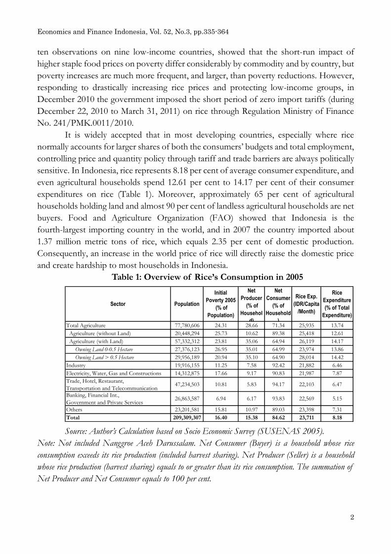
sensitive. In Indonesia, rice represents 8.18 per cent of average consumer expenditure, and
even agricultural households spend 12.61 per cent to 14.17 per cent of their consumer
expenditures on rice (Table 1). Moreover, approximately 65 per cent of agricultural
households holding land and almost 90 per cent of landless agricultural households are net
buyers. Food and Agriculture Organization (FAO) showed that Indonesia is the
fourth-largest importing country in the world, and in 2007 the country imported about
1.37 million metric tons of rice, which equals 2.35 per cent of domestic production.
Consequently, an increase in the world price of rice will directly raise the domestic price
and create hardship to most households in Indonesia.
Table 1: Overview of Rice’s Consumption in 2005
Total Agriculture 77,780,606 24.31 28.66 71.34 25,935 13.74
Agriculture (without Land) 20,448,294 25.73 10.62 89.38 25,418 12.61
Agriculture (with Land) 57,332,312 23.81 35.06 64.94 26,119 14.17
Owning Land 0-0.5 Hectare 27,376,123 26.95 35.01 64.99 23,974 13.86
Owning Land > 0.5 Hectare 29,956,189 20.94 35.10 64.90 28,014 14.42
Industry 19,916,155 11.25 7.58 92.42 21,882 6.46
Electricity, Water, Gas and Constructions 14,312,875 17.66 9.17 90.83 21,987 7.87
Trade, Hotel, Restaurant,
Transportation and Telecommunication47,234,503 10.81 5.83 94.17 22,103 6.47
Banking, Financial Int.,
Government and Private Services26,863,587 6.94 6.17 93.83 22,569 5.15
Others 23,201,581 15.81 10.97 89.03 23,398 7.31
Total 209,309,307 16.40 15.38 84.62 23,711 8.18
Rice
Expenditure
(% of Total
Expenditure)
Sector Population
Initial
Poverty 2005
(% of
Population)
Net
Producer
(% of
Househol
d)
Net
Consumer
(% of
Household
)
Rice Exp.
(IDR/Capita
/Month)
Source: Author’s Calculation based on Socio Economic Survey (SUSENAS 2005). Note: Not included Nanggroe Aceh Darussalam. Net Consumer (Buyer) is a household whose rice
consumption exceeds its rice production (included harvest sharing). Net Producer (Seller) is a household
whose rice production (harvest sharing) equals to or greater than its rice consumption. The summation of
Net Producer and Net Consumer equals to 100 per cent.
Economics and Finance Indonesia, Vol. 52, No.3, pp.335-364
3
According to the 2003 Agricultural Census, approximately 56 per cent of
agricultural household only own less than 0.5 hectares of land, meaning that many of them
are small and subsistence farmers. Thus, an increase in the rice price may not benefit them,
since their agricultural production is probably not sufficient to meet their needs. On the
contrary, a drop in the rice price will lower the incomes of farmers and create fewer jobs
for workers, particularly in the rural areas where a large share of employment depends on
the agricultural sector. According to the 2003 Agricultural Census, the agricultural sector
employs 46.34 million people, almost a half of total employment in Indonesia. About
one-fourth of them are engaged in rice paddy and crop activities. Hence, a price decrease
of rice and other crop commodities will directly cause suffering for about 11.6 million
farmers.
The impact of price volatility on poverty will certainly be very diverse, but the
average impact on poverty depends upon the balance between the two effects, both on
consumers and producers. There are many studies applying either a general or partial
equilibrium model concerning rice price and poverty in Indonesia. Leith et al. (2003), using
a general equilibrium representative household model found that an ad valorem increase in
the rice import tariff from 25 per cent to 45 per cent would increase poverty in both urban
and rural areas by 0.06 per cent and 0.04 per cent, respectively, in the medium-term. Warr
and Yusuf (2009), applying a general equilibrium multi household model, observed that
the main beneficiaries of the food price increases during 2007 to 2008 were not the poor,
but the owners of agricultural land and capital. In the case of rice, it showed that a 212 per
cent increase in real world rice prices did not have a significant effect on poverty in
Indonesia. This is because the increase in the rice price produces almost no increase in the
producer price of rice, or the output of rice, or its consumer price, and no reduction at all
in imports of rice. The reason is the (partially effective) ban on rice imports.
Warr (2005), utilizing a general equilibrium multi-household model, showed that a
90 per cent effective ban on Indonesia’s rice imports increases the poverty incidence in that country by a less than one per cent of the population. Utilizing a net benefit analysis
model, McCulloch (2008) found that high rice prices hurt the large majority of
Indonesians—perhaps 80 per cent—and benefit only a minority. Ikhsan (2003), using a
partial equilibrium model, found that a 10 per cent increase in the domestic rice price is
associated with a one per cent increase in poverty incidence.
Unlike the previous studies, this study aims at estimating the impact of the volatility
of the world price of rice and import tariffs of rice on poverty in Indonesia by applying a
computable general equilibrium-microsimulation approach (top-down approach) and also
the endogenous poverty line. It is expected that this study could identify comprehensively
who will benefit or lose from the change in the world rice price and import tariffs of rice.
The comprehensive results are valuable for policy makers in proposing an effective rice

Economics and Finance Indonesia, Vol. 52, No.3, pp.335-364
4
policy which could accommodate both consumers’ and producers’ interests. First, this study provides a brief overview of the rice policy in Indonesia. The next
part will explain the methodologies, including a computable general equilibrium
(CGE)-microsimulation model, the endogenous poverty line and the poverty calculation.
It will continue to analyze the impact of world rice price’s volatility and import tariff policy on poverty incidence. Like many CGE studies, this study is also complemented with the
sensitivity analysis to show the robustness of simulation results. This study will conclude
with some important findings and policy recommendations.
2. Overview of Rice Policy and Fluctuation of Rice Price in Indonesia
2.1 Rice Policy
Food policy in Indonesia is mainly dominated by rice policy. Three types of rice
policy could be distinguished: 1) pricing policy through price protection, 2) support
programs through subsidies, credits and training, and 3) investments in the rehabilitation,
improvement and extension of irrigated areas. By the end of the 1960s, BULOG, the
National Logistics Agency, was established to carry out three main mandates: stabilizing
price, controlling a national food security stock and distributing rice to the military and
civil servants on a monthly basis. However, after the 1998 financial crisis, the latter task
was abolished. The combination effect of three policies led to significant achievements, as
rice production doubled from 12 to 24 million tons between 1969 and 1983, while
self-sufficiency was attained in 1985.
In 1998, under the structural adjustments agreements with the International
Monetary Fund (IMF), BULOG’s monopoly was abolished and private companies were allowed to import rice. However, BULOG still accounted for around 75 per cent of total
rice imports. On September 22, 1998 rice imports were freed (that is, with a 0 per cent
tariff). On January 1, 2000, the Ministry of Trade began imposing tariffs on rice imports
of IDR (Indonesian Rupiah) 430 per Kg (equivalent to 21 per cent ad-valorem tariff at that
time). Based on BULOG’s recommendation, the Directorate General of Customs and Excise in September 2000 introduced a red lane inspection on rice imports in place,
meaning stricter standards of customs inspection than other food items (Leith et al., 2003).
In 2003, the import tariff was increased from IDR 430 per Kg to 750 per Kg, raising the ad
valorem equivalent tariff from 21 per cent to approximately 37 per cent (Warr, 2005). In
early 2004, a seasonal ban on rice imports was introduced.
Responding to a dramatic increase in the world rice price, in August 2007 the
government reduced the import tariff from IDR 750 per Kg to IDR 550 per Kg which
was again reduced to IDR 450 per Kg in December 2007. These policies were enacted by
the Ministry of Finance Regulations No. 180/PMK.011/2007 and
No.93/PMK.011/2007, respectively. The government again imposed a short period of
Economics and Finance Indonesia, Vol. 52, No.3, pp.335-364
5
zero import tariffs on rice starting from December 22, 2010 to March 31, 2011. This
policy was enacted through the Ministry of Finance Regulation No. 241/PMK.011/2010.
Starting from April 1, 2011, the import tariffs of rice were set again at IDR 450 per Kg. In
addition to tariff policies, the government also actively intervened in the rice market
through market operations, distributing raskin (cheap rice for the poor) and setting a floor
price for dry paddy (harga gabah kering giling).
2.2 Fluctuation of Rice Price
The world price and import tariff of rice can affect the domestic price of rice
following a simple formula: w
r
d
r
c
r PtPP 1 . Where, c
rP is consumer price of rice; d
rP
is domestic producer price of rice; w
rP is price of imported rice in foreign currency; is
proportion of domestic rice production to total domestic consumption; is proportion
of imported rice to total domestic consumption; t is import tariff of rice; and is
exchange rate USD/IDR. To what extent the world price can influence the domestic price
depends on the exchange rate, the share of imported rice in domestic consumption and
the import tariffs.
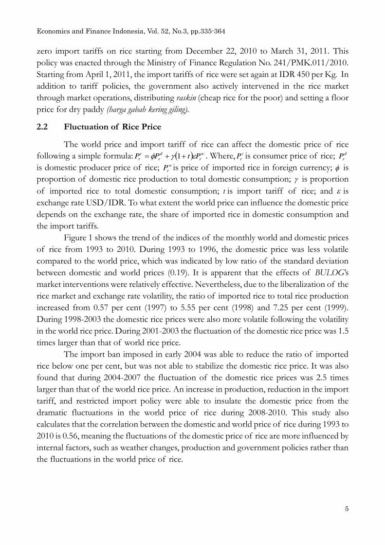
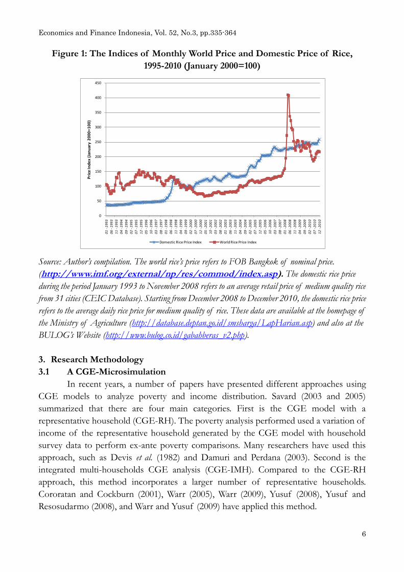
Figure 1 shows the trend of the indices of the monthly world and domestic prices
of rice from 1993 to 2010. During 1993 to 1996, the domestic price was less volatile
compared to the world price, which was indicated by low ratio of the standard deviation
between domestic and world prices (0.19). It is apparent that the effects of BULOG’s market interventions were relatively effective. Nevertheless, due to the liberalization of the
rice market and exchange rate volatility, the ratio of imported rice to total rice production
increased from 0.57 per cent (1997) to 5.55 per cent (1998) and 7.25 per cent (1999).
During 1998-2003 the domestic rice prices were also more volatile following the volatility
in the world rice price. During 2001-2003 the fluctuation of the domestic rice price was 1.5
times larger than that of world rice price.
The import ban imposed in early 2004 was able to reduce the ratio of imported
rice below one per cent, but was not able to stabilize the domestic rice price. It was also
found that during 2004-2007 the fluctuation of the domestic rice prices was 2.5 times
larger than that of the world rice price. An increase in production, reduction in the import
tariff, and restricted import policy were able to insulate the domestic price from the
dramatic fluctuations in the world price of rice during 2008-2010. This study also
calculates that the correlation between the domestic and world price of rice during 1993 to
2010 is 0.56, meaning the fluctuations of the domestic price of rice are more influenced by
internal factors, such as weather changes, production and government policies rather than
the fluctuations in the world price of rice.
Economics and Finance Indonesia, Vol. 52, No.3, pp.335-364
6
Figure 1: The Indices of Monthly World Price and Domestic Price of Rice,
1995-2010 (January 2000=100)
Source: Author’s compilation. The world rice’s price refers to FOB Bangkok of nominal price. (http://www.imf.org/external/np/res/commod/index.asp). The domestic rice price
during the period January 1993 to November 2008 refers to an average retail price of medium quality rice
from 31 cities (CEIC Database). Starting from December 2008 to December 2010, the domestic rice price
refers to the average daily rice price for medium quality of rice. These data are available at the homepage of
the Ministry of Agriculture (http://database.deptan.go.id/smsharga/LapHarian.asp) and also at the
BULOG’s Website (http://www.bulog.co.id/gabahberas_v2.php).
3. Research Methodology
3.1 A CGE-Microsimulation
In recent years, a number of papers have presented different approaches using
CGE models to analyze poverty and income distribution. Savard (2003 and 2005)
summarized that there are four main categories. First is the CGE model with a
representative household (CGE-RH). The poverty analysis performed used a variation of
income of the representative household generated by the CGE model with household
survey data to perform ex-ante poverty comparisons. Many researchers have used this
approach, such as Devis et al. (1982) and Damuri and Perdana (2003). Second is the
integrated multi-households CGE analysis (CGE-IMH). Compared to the CGE-RH
approach, this method incorporates a larger number of representative households.
Cororatan and Cockburn (2001), Warr (2005), Warr (2009), Yusuf (2008), Yusuf and
Resosudarmo (2008), and Warr and Yusuf (2009) have applied this method.
0
50
100
150
200
250
300
350
400
450
01
-1
99
3
06
-1
99
3
11
-1
99
3
04
-1
99
4
09
-1
99
4
02
-1
99
5
07
-1
99
5
12
-1
99
5
05
-1
99
6
10
-1
99
6
03
-1
99
7
08
-1
99
7
01
-1
99
8
06
-1
99
8
11
-1
99
8
04
-1
99
9
09
-1
99
9
02
-2
00
0
07
-2
00
0
12
-2
00
0
05
-2
00
1
10
-2
00
1
03
-2
00
2
08
-2
00
2
01
-2
00
3
06
-2
00
3
11
-2
00
3
04
-2
00
4
09
-2
00
4
02
-2
00
5
07
-2
00
5
12
-2
00
5
05
-2
00
6
10
-2
00
6
03
-2
00
7
08
-2
00
7
01
-2
00
8
06
-2
00
8
11
-2
00
8
04
-2
00
9
09
-2
00
9
02
-2
01
0
07
-2
01
0
12
-2
01
0
Pri
ce I
nd
ex
(Ja
nu
ary
20
00
=1
00
)
Domestic Rice Price Index World Rice Price Index

Economics and Finance Indonesia, Vol. 52, No.3, pp.335-364
7
The third approach is the CGE-Microsimulation approach (CGE-MS) which uses
a CGE model to generate prices that link to a micro-econometric household
microsimulation model. Chen and Ravallion (2003), Ikhsan et al. (2005), Boccafunso and
Savard (2006) and Dartanto (2009) utilized this approach to address many issues related to
poverty analysis. Lastly, the CGE-Household micro-simulation approach (CGE-HHS)
pioneered by Savard (2003 and 2005), which attempts to use the advantages of the
CGE-IMG and CGE-MS methods. CGE-HHS proposed to examine coherence between
the household model and the CGE model, introducing a bi-directional link and, therefore,
obtaining a converging solution between the two models.
This research will utilize the CGE-Microsimulation approach (CGE-MS) in order
to calculate how the volatility in rice prices in the international market and import tariffs
of rice influence poverty in Indonesia. This approach is applied because it provides
richness in household behavior, while remains extremely flexible in terms of specific
behaviors that can be modeled. The general idea of the CGE-MS approach is that a CGE
model feeds market and factor price changes into a microsimulation household model.
Chen and Ravallion (2003) used this methodology and built micro simulations on
economic assumptions that are consistent with the CGE model, notably that a household
takes prices as given and that those prices clear all markets. They also did not attempt to
assure full consistency between the micro-analysis and the CGE model’s predictions. There are five steps in calculating the impact of the volatility in world rice prices
and tariffs policy on poverty: First, calculating the initial condition of poverty utilizing the
2005 SUSENAS data (National Socio-Economic Survey), covering 64,407 households,
published by the Central Statistical Agency of Indonesia (Badan Pusat Statistik (BPS)).
Second, using the CGE model, simulating the impact of world price changes and import
tariffs of rice on domestic prices (including factor incomes). Third, entering data on the
increases in prices (including factors income) obtained from the CGE model into the
Susenas data set, to calculate the impact of the fluctuations in world price and import tariffs
on household welfare. This step is known as the microsimulation procedure. Fourth,
adjusting the poverty line using price changes obtained from the CGE in which the
poverty line becomes endogenous. Fifth, recalculating the poverty incidence using data
from steps three and four, and then compare it with the initial poverty incidence.
3.2 Indonesian Computable General Equilibrium
The General Equilibrium Theory follows the Walrasian tradition/Walras theory
that equilibrium prices and quantities are determined by the interaction between producers
and consumers in a perfectly competitive market. Consumers (or households) are assumed
to choose their consumption bundle to maximize their utility subject to the income
constraint. Producers (or firms) maximize their profits subject to production technology.
Economics and Finance Indonesia, Vol. 52, No.3, pp.335-364
8
The modern concept of the General Equilibrium Theory was provided by Kenneth Arrow,
Gerard Debreu and Lionel W. McKenzie in the 1950s.
Computable General Equilibrium (CGE) models are a class of economic models
that use actual economic data to estimate how an economy might react to changes in policy,
technology or other external factors. The static CGE model is built based on the extension
of the 2005 Indonesian Social Accounting Matrix (SAM) and follows the algorithm of the
International Food Policy Research Institute (IFPRI) standard CGE model developed by
Lofgren, Harris and Robinson (2001). The data used for the extension of SAM refers to
the 2005 Input-Output Table, the 2005 National Socio-Economic Survey, the Labor Force
Survey, and other sources.
Activities/Commodities
The extended 2005 Indonesian SAM has 26 industry/commodity categories: food
crops, soybeans, other crops, livestock, forestry, fishery, oil and metal mining, other mining
and quarrying, rice, food-beverage industry, textile-clothes-leather industry, wood
processing industry, pulp-paper and metal industry, chemical industry, electricity-gas-water,
construction, trade, restaurants, hotels, land transportation, air-water transportation and
telecommunication, warehousing, financial services, real estate, government and private
services, and individual/other services.
Factors of Production
The factors of production in this SAM are basically classified into five factors:
agricultural labor, production-operator-unskilled labor, sales and administration
(semi-skilled), skilled labor and non-labor factors, including land and capital. However,
each factor except the non-labor factor, is divided into two categories: rural and urban
labor. Hence, the factors of production consist of 9 categories overall.
Institutions and Households
There are three main institutions in the 2005 SAM: government, enterprises and
households. The representative household is basically divided into four categories:
agricultural households, non-agricultural households. Agricultural households are
classified into agricultural labor, agricultural households with less than 0.5 hectares of land,
agricultural households with land between 0.5 to 1 hectares, and agricultural household
with more than 1 hectare of land. Non-agricultural households are separated into rural
and urban households. Each category of households in the urban and rural grouping is
further classified into low-income, non-labor force households and high-income
households. Other accounts in the CGE model are the rest of the world (export-import),
saving-investment and taxation. Taxation is divided into indirect taxes, subsidies, income
Economics and Finance Indonesia, Vol. 52, No.3, pp.335-364
9
tax and import tariff.
Elasticity
The elasticity data used in this CGE refers to sources such as elasticity in the
Indonesian IFPRI CGE model2, Wayang model and other estimations of elasticity. The
Armington elasticities, the elasticity of substitution between imports and domestic output
in domestic demand, are 0.5 for all commodities except soybeans (1.5), rice (1.5), food
crops (1.5) and food and beverage industry (1.5). The constant elasticity of transformation
(CET) for domestic marketed output between exports and domestic supplies is set at 0.5
for all commodities except rice (1.5), soybeans (1.5), food crops (1.5), and food-beverage
industry (1.5). The elasticity of substitution (CES) between factors of production is 0.25
for all activities. The elasticity of substitution between aggregate factors and intermediate
input is 0.5 and the elasticity of output aggregation for commodities is 3. Household
consumption is modeled under the Linear Expenditure System (LES), whereby elasticities
vary between commodities, and is less than 1 for food products and more than 1 for
industrial products and services.
3.3 Microsimulation
The world prices and import tariffs of rice will influence household welfare
through changes in the price of domestic commodities and factor incomes. A
microsimulation procedure basically translates how price (factor income) changes from
the CGE can influence household welfare. This research modified Chen and Ravallion’s work (2003)3 to calculate the monetary value of household welfare changes in response to
changes in prices and factor incomes. Increasing prices would reduce households’ ability to afford an initial bundle of consumption while increasing factor incomes would increase
household incomes. An increase in income means an increase in the ability to consume
more. The formula for household welfare change is shown below:
1
111
)(l l
lill
n
k k
kikk
m
j j
j
ijijjir
drKr
w
dwLw
p
dpsqpW (1)
Where, iW is the welfare change of household-i, i: 1,2,3,…,64,407; ijq is the quantity of
product-j consumed by household-i, j=1,2,3,…,26; product-j refers to classification in the
CGE model; ijs is the quantity of product-j provided/supplied by household-i; )( ijij sq is
the net consumption of product-j which must be bought by household-i. According to 2 Presentation Material of CGE Training at Department of Economics, University of Indonesia in 2002 3 This formula is derived from the maximizing behavior of both consumer and producer, using the envelope theorem (see Chen and Ravallion, 2003).
Economics and Finance Indonesia, Vol. 52, No.3, pp.335-364
10
SUSENAS data set, the value of household consumption is always larger than or equal to
the value of household production ijij sq ; jp
is the price of product-j; jdpis price
change of product-j; ikL is the labor supply of household-i in sector-k; sector-k refers to a
labor category in the CGE model; kw is wage in sector-k; kdw is the wage change in
sector-k; ilK is the non-labor endowment of household-i; lr is the rate of return; and ldr is
the change in the rate of return.
The change of household welfare is the sum of the change in household
expenditure and household income. The negative sign in the first part of the formula
indicates that increasing prices will increase household expenditure, and consequently
lower household welfare. Conversely, the positive signs of the last two parts of the
formula indicate that increasing wages and the non-labor rate of return will increase
household income, and thus increase household welfare. This study assumes that the
consumption pattern of households do not change following the price change. This
assumption might be unrealistic in the long run. However, due to the lack of information
about the elasticity of substitution and also to simplify the model, this study is forced to
assume ―no change in the consumption pattern‖ to calculate the household welfare
change.
The model also assumes that the change of household welfare will directly
influence household consumption (expenditure) and there is no saving activity, i.e.
households are not allowed to save the net welfare. The new expenditure function is
shown as below:
iijiiijji WypEWydppE ),())(),((00000 (2)
))(),((00 iijji WydppE is household-i’s expenditure after the simulations in the world
prices and import tariffs of rice; ),(000 iji ypE is the initial household-i’s expenditure; jp
0is
the initial vector price and iy0 is the initial endowment/income of household-i.
))(),((00 iijji WydppE is used to calculate the new poverty incidence.
3.4 Endogenous poverty line and poverty calculation
BPS (the Central Statistical Agency of Indonesia) uses 2,100 calories/capita/day
Economics and Finance Indonesia, Vol. 52, No.3, pp.335-364
11
from 52 commodities to calculate the food poverty line. The food poverty line is
heterogeneous among regions due to differences in food prices and consumption patterns
among regions. To obtain the poverty line, expenditure on food must be added with
non-food expenditures, such as health, education, transportation, etc.
The increasing commodity price would also increase the money metric of
obtaining 2,100 calories, therefore the poverty line will become endogenous following a
variation in relative prices (Decaluwe, Savard and Thorbecke, 2005). Hence, the initial
food poverty line should be adjusted with the price change of food products in proportion
to the share of those products in the poverty line; and also be adjusted with the price
change of non-food products. This study assumes that the composition of commodities
in the poverty line does not change following the change in prices. This assumption
follows the fact that the commodities in the poverty line are basic need products which are
price inelastic. It also observes that the composition and quantity of commodities in the
poverty line do not much change from SUSENAS 2002, 2005 and 2008. Therefore, the
new poverty line that changes following a variation in prices is known as the endogenous
of poverty line that theoretically can be calculated as follows:
nf
nfm
nf
nfnf
f
fn
f
ffp
dpp
p
dppz 11
11
(3)
Where, z is the poverty line;
f
f
ffp1
is the food poverty line;
nf
nf
nfnfp1
is the non-food
poverty line; fp is the food price-f, f=1,…,n; f is the minimum consumption of food
product-f; fdp is the change in food price-f, f=1,…,n; nfp is the non-food price-nf,
nf=1,…,m; nf is the minimum consumption of non-food product-nf, nf=1,..,m; nfdp is the
change in non-food price-nf, nf=1,…,m. However, the Central Statistical Agency (BPS) only annually publishes the
aggregate value of the food poverty line (PFL) and the non-food poverty line (NFPL) for
each province at the rural and urban level; therefore, equation (3) is modified as below:
pr
pr
pr
pr
pr
prprprNFP
NFPNFPL
FP
FPFPLPLz
0
0
0
011 (4)
Where, prpr PLz is the poverty line in province-p, p=1,…,30, at region-r, r=urban and rural;
prFPL0 is the initial food poverty line in province-p at region-r; prFP is the change in

Economics and Finance Indonesia, Vol. 52, No.3, pp.335-364
12
composite food price in province-p at region-r; prFP0
is the initial composite food price in
province-p at region-r; rNFPL0
is the initial non-food poverty line in province-p at region-r;
prNFP is the change in composite non-food price in province-p at region-r; and prNFP0
is the
initial composite non-food price in province-p at region-r.
The price changes for either food or non-food prices are the same across all regions,
because the CGE model can only produce price and factor income changes at the national
level. The composite prices of either food or non-food products are calculated based on the
composition of consumption in the 2005 Social Accounting Matrix and in the 2005
SUSENAS data set. By 2005, the monthly monetary value of the national poverty line was
IDR 117,259 in rural areas ($11.7) and IDR 150,799 ($15) in urban areas. BPS is updating the
poverty line for each province every year. The 2005 provincial poverty line and simulated
changes in the poverty line under various changes in the world rice price and import tariffs
are shown in Appendix 4.
In order to calculate poverty, this study applies the FGT (Foster, Greer and
Thorbecke, 1984) formula. The modified formula is shown below:
q
i r
irr
PL
EPL
nHC
1
1
(5)
Where, HC is the head count index (poverty incidence); n is the number of population; i
is the individual-i; rPL is the poverty line in region-r; irE is the expenditure of individual-i
in region-r; q is the number of individuals below or at the poverty line; and is the
parameter for the FGT. When is zero, the poverty measurement is the headcount index
which represents the percentage of population below the poverty line. The poverty-gap
index, PG, which measures the depth of poverty, is calculated by setting to 1 and the
squared poverty gap is obtained with equal to 2. This study focuses only on analyzing the
head count index and the poverty gap index.
3.5 Scenarios Simulations
The aim of simulations is to find out how much change occurred in the poverty
under the various scenarios of the world prices and import tariffs of rice. The scenarios
simulations are done referring to the fact that the world price of rice could sharply
increase (decrease) only in short period. In 2008, the monthly world price of rice could
increase or decrease in the range from -17.31 per cent to 50.93 per cent. In addition, the

Economics and Finance Indonesia, Vol. 52, No.3, pp.335-364
13
government also actively intervenes in the domestic rice market through changing the
import tariffs of rice. It is counted that the effective import tariff of rice in the 2005 SAM
is equivalent to 5.6 per cent; thus a decrease in the import tariff from IDR 750/Kg to IDR
450/kg as a response to a dramatic increase in the world rice prices is identical to a
decrease of 40 per cent of the effective import tariff. This is equal to a decrease of the
import tariff from 5.6 per cent to 3.36 per cent. As mentioned before, in December 2010
the government again imposed a zero import tariff on rice.
The simulations are done under several scenarios which are basically divided into
four categories: first, simulating an increase in the world rice price by 20 per cent, 40 per
cent, 60 per cent, 80 per cent and 100 per cent; second, simulating a decrease in world rice
prices by 20 per cent, 40 per cent, 60 per cent and 80 per cent4 respectively; third,
simulating various decreases in import tariffs on rice by 20 per cent, 40 per cent, 60 per
cent, 80 per cent and 100 per cent respectively; lastly, simulating various increases in
import tariffs on rice by 20 per cent, 40 per cent, 60 per cent, 80 per cent and 100 per cent
respectively. Various simulations are conducted in order to ascertain the sensitivity of
poverty in respect to the change in world prices and import tariffs.
The simulations are done under the following closure rules: investment driven
saving, flexible government saving and fixed direct tax rates, flexible exchange rates and
fixed foreign saving, fixed capital formation, labor fully employed and mobile across
activities, capital fully employed and activity-specific and fixed domestic producer price
(price numeraire).
4. The Impact of World Rice Prices and Import Tariffs on Poverty in Indonesia
4.1 CGE Result
4.1.1 Changes in Macroeconomic Indicators, Consumer Prices and Factor
Incomes
Generally, an increase (decrease) in world rice prices will be followed by a decrease
(increase) in macroeconomic indicators, such as private consumption, imports, net indirect
tax, exports and gross domestic product (GDP), while the consumer price index (CPI)
moves in the same direction to change the world prices (Appendix 1). The simulation
results shows that a 60 per cent increase in world rice prices decreases private
consumptions by 0.107 per cent, imports by 0.201 per cent, net indirect tax by 0.439 per
cent, exports by 0.031 per cent and GDP by 0.032 per cent, while increasing CPI by 0.431
per cent. An increase in the CPI depletes households’ welfare that in the end decreases
household (private) consumptions as well as GDP. The same magnitude of change in
macroeconomic indicators is also observed on increases (decreases) in the import tariffs
4 We did not simulate a 100 per cent decrease in the world rice price. This is because a 100 per cent decrease means the world rice price equal to 0 which is impossible in the CGE’s simulation.
Economics and Finance Indonesia, Vol. 52, No.3, pp.335-364
14
on rice.
An increase (decrease) in the world rice price would decrease (increase) the
composite good supply in the domestic market. A 60 per cent increase in the world price
leads to a decline in the composite supply of rice by 0.93 per cent. Theoretically, an
increase in import prices reduces demand for imported goods and provides incentives to
domestic producers to raise production. However, due to the lack of flexibility in domestic
production of rice to respond to price increases, an increase in the domestic production of
rice is unable to fill a gap of composite supply resulting from massive decreases in
imported rice. Hence, the composite rice supply declines below the previous level.
Turning to changes in consumer price and factor incomes, the CGE simulations
shows that an increase in the world prices of rice by 20 per cent, 40 per cent, 60 per cent,
80 per cent and 100 per cent raises the domestic consumer price of rice by 2.49 per cent,
4.60 per cent, 6.30 per cent, 8.00 per cent and 9.40 per cent respectively. Moreover, if the
world price decreases by 20 per cent, 40 per cent, 60 per cent and 80 per cent, the domestic
price of rice decreases by 2.92 per cent, 6.76 per cent, 12.07 per cent and 20.96 per cent
respectively (Appendix 2). The domestic price is apparently sensitive to the decrease in the
world price of rice since the volume of imported rice tends to increase when the world
price decrease.
An increase in the world price of rice is advantageous only for non labor factors
(capital or land). All labor categories are worse off under this condition due to a sharp
decrease in average wage rates. In contrast, all labor categories are better off if the world
rice price decrease up to 40 per cent. However, a high decrease in the world rice price of
more than 60 per cent adversely affects agricultural labor due to declining wage rates
(Appendix 3). This contradicts to what many theories predict that agricultural labor should
benefit (suffer) from an increase (decrease) in the world rice prices, because responding to
the rise in the domestic price of rice as a result of an increase in the world prices,
households might choose or combine three alternatives: 1) allocating more resources to
afford rice through reduced consumption of others products, 2) reducing consumption of
rice and 3) substituting rice for other products. These three alternatives would affect the
decrease in aggregate demand in an economy that would be followed by decreasing factor
incomes.
On the other hand, the reduction of import tariffs by 20 per cent, 40 per cent, 60
per cent, 80 per cent and 100 per cent will lower the domestic price of rice by 0.30 per cent,
0.70 per cent, 1.10 per cent, 1.40 per cent and 1.90 per cent respectively. This policy is able
to raise the average incomes of all factors of production, except for non labor factor
varying from 0.017 per cent to 0.301 per cent. Meanwhile, the increase in import tariffs at
the same rate can raise the domestic price of rice by 0.40 per cent, 0.70 per cent, 1.00 per
cent, 1.40 per cent and 1.70 per cent respectively. An increase in the import tariffs at any
Economics and Finance Indonesia, Vol. 52, No.3, pp.335-364
15
level will increase wage rates of agricultural labors and the returns of non-labor factor.
However, all labor categories, except agricultural labor, are worse off when responding to
an increase in the import tariffs. Agricultural labor is the only factor that consistently gets
benefits from any increase or decrease in the import tariffs. These simulation results
appear to contradict the common belief that a decrease in the import tariffs of rice would
adversely affect labor in the agriculturalal sector, because a decrease in the import tariffs of
rice lowers the domestic rice prices driving up the domestic consumption of both non
agricultural and agricultural products and at the end bidding up the wage rates of all labor
factors.
According to the CGE simulations, there are differences in the percentage change
of domestic consumer prices when the world rice prices (import tariffs) increase or
decrease at the same percentage points. For instance, a 60 per cent increase (decrease) in
the world price will be followed by a 6.3 per cent increase (12.07 per cent decrease) in the
domestic consumer price of rice. Declines in world rice prices directly decrease domestic
rice prices through lowering the imported rice prices and dropping the domestic prices as
consequence of excess supply in the domestic market. The other transmission is that a
decrease in the price of domestic rice lowers the real incomes of those selling rice. When
incomes fall, goods and services will be demanded less, and domestic price will decline. On
the contrary, increases in the world rice price directly raise the imported rice price as well as
the domestic rice price. Unfortunately, a high price of domestic rice forces households to
reduce their demand and in the end lowers its price. Therefore, in the case of a world price
decrease, both direct and indirect effects move in the same direction; while in the case of a
world price increase, the direct and indirect effect cancel out each other. Hence, this clearly
shows that a change in domestic prices in response to a decrease in world prices is larger
than the response to an increase in world prices.
4.2 CGE-Microsimulation Analysis
4.2.1 World Rice Prices and Poverty
In a CGE-Microsimulation analysis, the impact of world price volatility and
import tariffs of rice on poverty solely depends on how large the effect of these shocks on
changing the price level and factors income in the economy are. However, how large the
price changes, including factors income, can influence the poverty incidence depends on
the poor’s consumption pattern and the poor’s source of income. It also depends on how sensitive the poverty line is in responding to the price change.
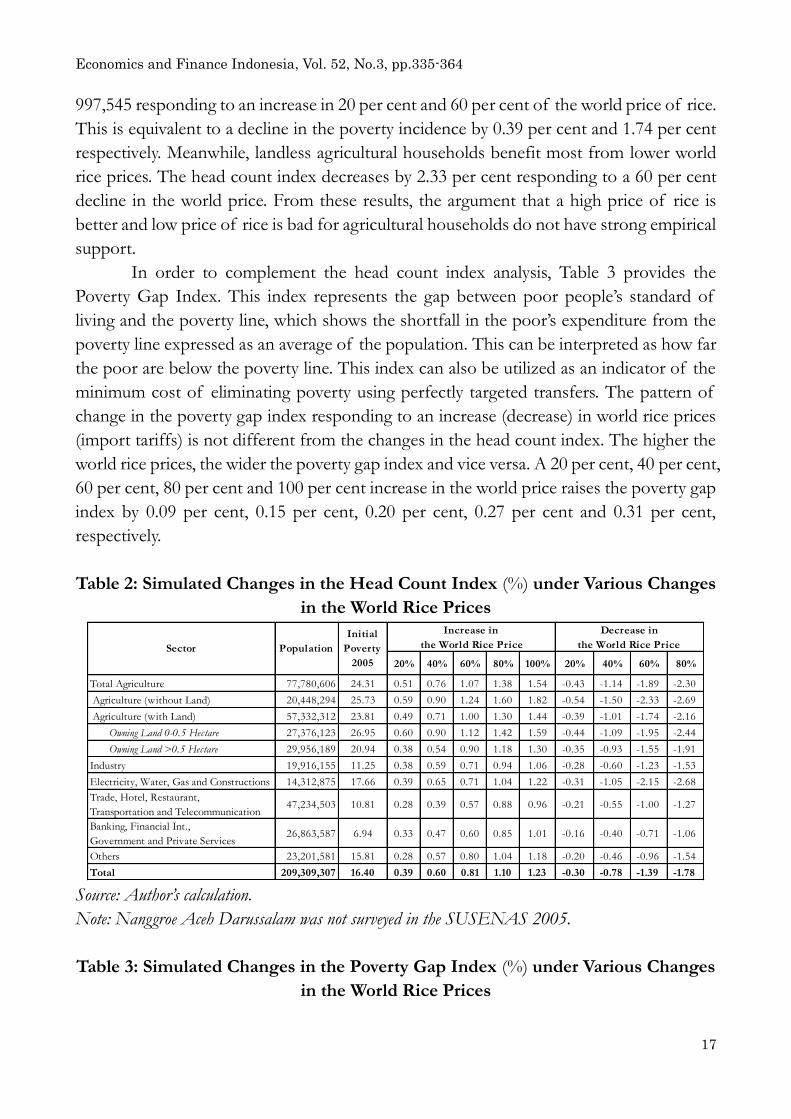
Table 2 summarizes the impact of various world prices and import tariffs of rice
on poverty in Indonesia. As many other imported countries, an increase in the world prices
of rice raises the incidence of poverty, while a decrease in the world price also reduces
poverty. The 20 per cent, 40 per cent, 60 per cent, 80 per cent and 100 per cent respectively

Economics and Finance Indonesia, Vol. 52, No.3, pp.335-364
16
of an increase in the world price raises poverty by 819,189; 1,245,530; 1,687,270;
2,292,026; and 2,581,536 respectively. This is equivalent to an increase in the poverty
index by 0.39 per cent, 0.60 per cent, 0.81 per cent, 1.10 per cent and 1.23 per cent
respectively. On the other hand, a decline in the world price of rice at any rate is good for
all household categories. The decrease in the world price at 20 per cent, 40 per cent, 60 per
cent and 80 per cent respectively reduces poverty by 622,857; 1,628,371; 2,910,403; and
3,719,739 respectively which are equal to a decrease in the poverty index by 0.30 per cent,
0.78 per cent, 1.39 per cent and 1.78 per cent respectively. The fluctuations in the world
rice price and the poverty incidence move in the same direction. However, the elasticity of
poverty in relation to the world rice price is not constant and decreases in line with the
higher price change.
At the disaggregate level, all household categories, agricultural and
non-agricultural, suffer from an increase in the world rice price. Landless agricultural
households suffer most from an increase in the world price. If the world price rises by 40
per cent, the head count index rises by 0.90 per cent. In terms of absolute numbers,
poverty increases are more frequently observed among small landowners of agricultural
households. An increase of 40 per cent in the world price raises the number of poor by
247,061. Landless households and small landowning households are basically low-income
groups characterized by a high proportion of their expenditure on rice and a high
dependency on agricultural activity as a main source of income. Therefore, a sudden
increase in rice prices to unaffordable level adversely affects these groups.
These simulations show that, in contrast to what many theories predict,
households working in the agricultural sector do not benefit from an increase in the world
price of rice, because of the high proportion of their budgets going towards rice,
subsistence level of production and rigidity in the domestic production of rice in response
to an increase in price. BPS reports that even though the budgeted share on food has been
continuously decreasing since 1999, food expenditure in 2009 still represented 50.62 per
cent of average consumer expenditure, which is mostly spent on food crops. An increase
in the world rice prices that suddenly increases the domestic rice prices forces agricultural
households to choose two difficult options - either reduce food consumption or use
substitutes. However, substitution is not a feasible option because rice consumption is
related to taste and customs. Even though agricultural households benefit through a
gradual increase in the wages of agricultural labor, it can only compensate partially for the
increase in expenditure as a result of price increases. Therefore, increases in world
commodity prices hurt agricultural households rather than benefits them.
On the other hand, the decrease of world price of rice at any level is advantageous
not only for non-agricultural households, but also for agricultural households with and
without land. The poverty of agricultural households with land declines by 224,551 and
Economics and Finance Indonesia, Vol. 52, No.3, pp.335-364
17
997,545 responding to an increase in 20 per cent and 60 per cent of the world price of rice.
This is equivalent to a decline in the poverty incidence by 0.39 per cent and 1.74 per cent
respectively. Meanwhile, landless agricultural households benefit most from lower world
rice prices. The head count index decreases by 2.33 per cent responding to a 60 per cent
decline in the world price. From these results, the argument that a high price of rice is
better and low price of rice is bad for agricultural households do not have strong empirical
support.
In order to complement the head count index analysis, Table 3 provides the
Poverty Gap Index. This index represents the gap between poor people’s standard of living and the poverty line, which shows the shortfall in the poor’s expenditure from the poverty line expressed as an average of the population. This can be interpreted as how far
the poor are below the poverty line. This index can also be utilized as an indicator of the
minimum cost of eliminating poverty using perfectly targeted transfers. The pattern of
change in the poverty gap index responding to an increase (decrease) in world rice prices
(import tariffs) is not different from the changes in the head count index. The higher the
world rice prices, the wider the poverty gap index and vice versa. A 20 per cent, 40 per cent,
60 per cent, 80 per cent and 100 per cent increase in the world price raises the poverty gap
index by 0.09 per cent, 0.15 per cent, 0.20 per cent, 0.27 per cent and 0.31 per cent,
respectively.
Table 2: Simulated Changes in the Head Count Index (%) under Various Changes
in the World Rice Prices
20% 40% 60% 80% 100% 20% 40% 60% 80%
Total Agriculture 77,780,606 24.31 0.51 0.76 1.07 1.38 1.54 -0.43 -1.14 -1.89 -2.30
Agriculture (without Land) 20,448,294 25.73 0.59 0.90 1.24 1.60 1.82 -0.54 -1.50 -2.33 -2.69
Agriculture (with Land) 57,332,312 23.81 0.49 0.71 1.00 1.30 1.44 -0.39 -1.01 -1.74 -2.16
Owning Land 0-0.5 Hectare 27,376,123 26.95 0.60 0.90 1.12 1.42 1.59 -0.44 -1.09 -1.95 -2.44
Owning Land >0.5 Hectare 29,956,189 20.94 0.38 0.54 0.90 1.18 1.30 -0.35 -0.93 -1.55 -1.91
Industry 19,916,155 11.25 0.38 0.59 0.71 0.94 1.06 -0.28 -0.60 -1.23 -1.53
Electricity, Water, Gas and Constructions 14,312,875 17.66 0.39 0.65 0.71 1.04 1.22 -0.31 -1.05 -2.15 -2.68
Trade, Hotel, Restaurant,
Transportation and Telecommunication47,234,503 10.81 0.28 0.39 0.57 0.88 0.96 -0.21 -0.55 -1.00 -1.27
Banking, Financial Int.,
Government and Private Services26,863,587 6.94 0.33 0.47 0.60 0.85 1.01 -0.16 -0.40 -0.71 -1.06
Others 23,201,581 15.81 0.28 0.57 0.80 1.04 1.18 -0.20 -0.46 -0.96 -1.54
Total 209,309,307 16.40 0.39 0.60 0.81 1.10 1.23 -0.30 -0.78 -1.39 -1.78
Sector Population
Initial
Poverty
2005
Increase in
the World Rice Price
Decrease in
the World Rice Price
Source: Author’s calculation. Note: Nanggroe Aceh Darussalam was not surveyed in the SUSENAS 2005.
Table 3: Simulated Changes in the Poverty Gap Index (%) under Various Changes
in the World Rice Prices

Economics and Finance Indonesia, Vol. 52, No.3, pp.335-364
18
20% 40% 60% 80% 100% 20% 40% 60% 80%
Total Agriculture 77,780,606 4.93 0.13 0.20 0.28 0.38 0.44 -0.11 -0.26 -0.46 -0.57
Agriculture (without Land) 20,448,294 5.52 0.15 0.24 0.33 0.45 0.52 -0.14 -0.32 -0.55 -0.71
Agriculture (with Land) 57,332,312 4.71 0.12 0.19 0.26 0.35 0.41 -0.10 -0.24 -0.43 -0.52
Owning Land 0-0.5 Hectare 27,376,123 5.44 0.14 0.22 0.29 0.40 0.46 -0.11 -0.27 -0.48 -0.60
Owning Land >0.5 Hectare 29,956,189 4.05 0.11 0.17 0.23 0.31 0.36 -0.09 -0.21 -0.38 -0.46
Industry 19,916,155 2.10 0.07 0.11 0.15 0.21 0.24 -0.06 -0.14 -0.26 -0.35
Electricity, Water, Gas and Constructions 14,312,875 3.01 0.10 0.17 0.23 0.31 0.36 -0.10 -0.23 -0.40 -0.51
Trade, Hotel, Restaurant,
Transportation and Telecommunication47,234,503 2.01 0.07 0.10 0.14 0.19 0.21 -0.05 -0.13 -0.24 -0.30
Banking, Financial Int.,
Government and Private Services26,863,587 1.36 0.05 0.09 0.11 0.16 0.19 -0.05 -0.10 -0.19 -0.28
Others 23,201,581 3.40 0.09 0.14 0.19 0.26 0.30 -0.07 -0.18 -0.33 -0.43
Total 209,309,307 3.24 0.09 0.15 0.20 0.27 0.31 -0.08 -0.19 -0.34 -0.43
Sector Population
Initial
Poverty
Gap Index
2005
Increase in
the World Rice Price
Decrease in
the World Rice Price
Source: Author’s calculation. Note: Nanggroe Aceh Darussalam was not surveyed in the SUSENAS 2005.
4.2.2 Import Tariff Policies and Poverty
The impact of import tariffs of rice on poverty is not that much different in
pattern with the impact of world price volatility of rice on poverty. Table 4 shows that an
increase in import tariffs of rice by 20 per cent, respectively 40 per cent, 60 per cent, 80 per
cent and 100 per cent will be followed by an increase in poverty by 141,900; 215,060;
312,875; 474,441; and 578,952 persons which equals to an increase in the poverty
incidence by 0.07 per cent, 0.10 per cent, 0.15 per cent, 0.23 per cent and 0.28 per cent
respectively. Both landless and landholder households are worse off responding to an
increase in import tariffs. If the import tariffs of rice increase by 20 per cent, those
working in the trade-hotels-restaurants and transportation sectors suffer most. However,
the high protection on agricultural sectors, i.e. 100 per cent increase in the import tariff of
rice, intended to help agricultural producers, will result in the opposite direction. The
poverty index of this group rises by 0.36 per cent. On the other hand, generally most of
the households acquire benefits from lower import tariffs. The number of poverty will be
reduced by 68,694; 161,546; 258,569; 293,618; and 390,160 persons responding to the
decrease in import tariffs of rice by 20 per cent, 40 per cent, 60 per cent, 80 per cent and
100 per cent (zero import tariffs) respectively. The numbers are equivalent to the decrease
in the poverty index by 0.03 per cent, 0.08 per cent, 0.12 per cent, 0.14 per cent and 0.19
per cent respectively.
Table 4 shows three important findings: first, both a 40 per cent decrease in the
effective import tariff of rice enacted by Regulation No. 180/PMK.011/2007 and
No.93/PMK.011/2007 in response to high world rice price during 2007 to 2009 and the
zero import tariffs implemented by regulation No. 241/PMK.011/2010 in response to

Economics and Finance Indonesia, Vol. 52, No.3, pp.335-364
19
high world prices in 2010 could not perfectly absorb the negative impact of rising world
rice prices on poverty in Indonesia. Second, high import tariffs on rice, intended to help
agricultural producers, does not have strong empirical support. Third, a surprising finding
was that agricultural households, whether they own land or not, will benefit from lower
import tariffs and suffer from higher import tariffs. This appears to contradict a common
belief that a decrease in import tariffs would cause suffering for agricultural households
while an increase in import tariffs would be advantageous for agricultural households.
Theoretically, increases in import tariffs have two effects: an income effect from an
increase in incomes of those who sell either rice or agricultural labor, and the price effect
which results from an increase in the price of rice. It is observed that the price effect is
more dominant than the income effect when import tariffs either increase or decrease.
Similar to the earlier finding, this is due to the high budget share of food and rigidities in
domestic production of rice in response to an increase in price. Therefore, both landless
agricultural households and landowning agricultural households are worse off in the
presence of high import tariffs on rice.
Table 5 shows changes in the poverty gap index under various changes in the
import tariffs of rice. A 20 per cent, 40 per cent, 60 per cent, 80 per cent and 100 per cent
decrease in the import tariffs reduce the poverty gap index by 0.02 per cent, 0.03 per cent,
0.04 per cent, 0.05 per cent and 0.06 per cent, respectively. The poverty gap index of some
groups, such as industry and service employees, does not change in response to a decrease
in import tariffs of rice up to 20 per cent. This shows that the poverty gap index is
insensitive to a change in the import tariffs of rice because adjustments in the import
tariffs have little effect on changing prices and factor incomes in the economy.
Table 4: Simulated Changes in the Head Count Index (%) under Various Changes
in the Import Tariffs of Rice
20% 40% 60% 80% 100% 20% 40% 60% 80% 100%
Total Agriculture 77,780,606 24.31 0.06 0.12 0.19 0.29 0.36 -0.02 -0.09 -0.18 -0.20 -0.25
Agriculture (without Land) 20,448,294 25.73 0.09 0.13 0.26 0.34 0.47 -0.04 -0.11 -0.26 -0.26 -0.33
Agriculture (with Land) 57,332,312 23.81 0.05 0.12 0.17 0.28 0.32 -0.01 -0.09 -0.14 -0.18 -0.22
Owning Land 0-0.5 Hectare 27,376,123 26.95 0.10 0.18 0.23 0.40 0.45 0.00 -0.07 -0.15 -0.19 -0.23
Owning Land > 0.5 Hectare 29,956,189 20.94 0.01 0.06 0.10 0.16 0.21 -0.03 -0.10 -0.14 -0.17 -0.21
Industry 19,916,155 11.25 0.04 0.07 0.11 0.17 0.18 -0.02 -0.06 -0.11 -0.11 -0.18
Electricity, Water, Gas and Constructions 14,312,875 17.66 0.05 0.06 0.10 0.19 0.34 -0.12 -0.17 -0.17 -0.17 -0.22
Trade, Hotel, Restaurant,
Transportation and Telecommunication47,234,503 10.81 0.10 0.12 0.15 0.22 0.25 -0.03 -0.05 -0.10 -0.11 -0.14
Banking, Financial Int.,
Government and Private Services26,863,587 6.94 0.03 0.07 0.13 0.16 0.16 -0.03 -0.03 -0.03 -0.05 -0.10
Others 23,201,581 15.81 0.09 0.09 0.10 0.16 0.21 -0.04 -0.09 -0.09 -0.11 -0.15
Total 209,309,307 16.40 0.07 0.10 0.15 0.23 0.28 -0.03 -0.08 -0.12 -0.14 -0.19
Sector Population
Initial
Poverty
2005
Decrease in
the Import Tariffs of Rice
Increase in
the Import Tariffs of Rice
Source: Author’s calculation.

Economics and Finance Indonesia, Vol. 52, No.3, pp.335-364
20
Note: Nanggroe Aceh Darussalam was not surveyed in the SUSENAS 2005.
Table 5: Simulated Changes in the Poverty Gap Index (%) under Various Changes
in the Import Tariffs of Rice
20% 40% 60% 80% 100% 20% 40% 60% 80% 100%
Total Agriculture 77,780,606 4.93 0.02 0.03 0.05 0.07 0.09 -0.01 -0.02 -0.04 -0.05 -0.07
Agriculture (without Land) 20,448,294 5.52 0.02 0.04 0.05 0.08 0.10 -0.01 -0.03 -0.05 -0.06 -0.08
Agriculture (with Land) 57,332,312 4.71 0.02 0.03 0.05 0.06 0.08 0.00 -0.02 -0.03 -0.04 -0.06
Owning Land 0-0.5 Hectare 27,376,123 5.44 0.03 0.04 0.05 0.07 0.09 0.00 -0.02 -0.04 -0.05 -0.07
Owning Land > 0.5 Hectare 29,956,189 4.05 0.02 0.03 0.04 0.06 0.07 0.00 -0.02 -0.03 -0.04 -0.06
Industry 19,916,155 2.10 0.01 0.02 0.03 0.04 0.05 0.00 -0.01 -0.02 -0.03 -0.03
Electricity, Water, Gas and Constructions 14,312,875 3.01 0.02 0.03 0.04 0.05 0.07 -0.01 -0.02 -0.04 -0.05 -0.06
Trade, Hotel, Restaurant,
Transportation and Telecommunication47,234,503 2.01 0.01 0.02 0.02 0.03 0.04 0.00 -0.01 -0.02 -0.02 -0.03
Banking, Financial Int.,
Government and Private Services26,863,587 1.36 0.01 0.01 0.02 0.03 0.03 0.00 -0.01 -0.02 -0.02 -0.03
Others 23,201,581 3.40 0.02 0.03 0.04 0.05 0.06 0.00 -0.01 -0.02 -0.03 -0.04
Total 209,309,307 3.24 0.02 0.03 0.04 0.05 0.06 0.00 -0.02 -0.03 -0.04 -0.05
Sector Population
Initial
Poverty
Gap Index
2005
Increase in
the Import Tariffs of Rice
Decrease in
the Import Tariffs of Rice
Source: Author’s calculation. Note: Nanggroe Aceh Darussalam was not surveyed in the SUSENAS 2005.
5. Sensitivity Analysis
The CGE estimation results are known to be sensitive to the values of the
Armington elasticities. However, there have been few empirical studies on estimating these
elasticities. Many studies show that the resulting estimates of these elasticities varied widely.
McDaniel and Balistreri (2003) confirmed that the wide range estimates of Armington
elasticities depend on the data used, disaggregating sector and methodology applied.
Many CGE studies in Indonesia also applied a wide range of Armington elasticity
on Rice. Indonesian IFPRI CGE Model, Leith et al. (2003), Warr (2005), Warr (2009), Warr
and Yusuf (2009) assumed the Armington elasticity to be 10, 6, 6, 6 and 6 respectively.
However, Warr (2008) estimated that though imported and domestically produced rice are
considered relatively close substitutes in the demand in Indonesia, the Armington elasticity
ranges from 2 to 5. For comparison, Kapuschinki and Warr (1999) found that the
estimated Armington elasticities of the Philippines’ economy range from 0.2 for metal
product to 4 for sugar milling and refining and particularly for rice, the elasticity ranges
from 0.61 to 2.05 depending on the methodology applied.
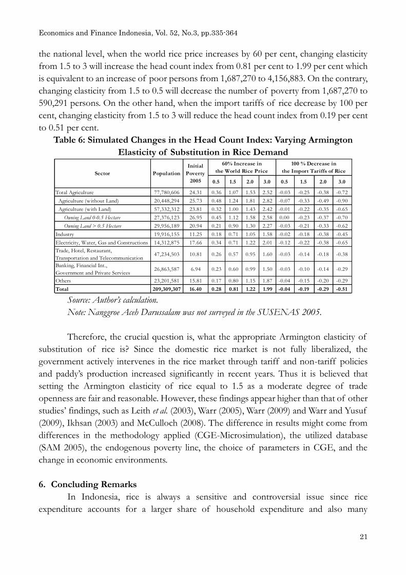
Table 6 shows that the impact of a 60 per cent increase in the world rice price and
a 100 per cent decrease in the import tariffs of rice on poverty (zero import tariffs) are
slightly sensitive to the variation of Armington elasticity. An increase (decrease) in the
Armington elasticity will be followed by an increase (decrease) in the poverty incidence. At
Economics and Finance Indonesia, Vol. 52, No.3, pp.335-364
21
the national level, when the world rice price increases by 60 per cent, changing elasticity
from 1.5 to 3 will increase the head count index from 0.81 per cent to 1.99 per cent which
is equivalent to an increase of poor persons from 1,687,270 to 4,156,883. On the contrary,
changing elasticity from 1.5 to 0.5 will decrease the number of poverty from 1,687,270 to
590,291 persons. On the other hand, when the import tariffs of rice decrease by 100 per
cent, changing elasticity from 1.5 to 3 will reduce the head count index from 0.19 per cent
to 0.51 per cent.
Table 6: Simulated Changes in the Head Count Index: Varying Armington
Elasticity of Substitution in Rice Demand
0.5 1.5 2.0 3.0 0.5 1.5 2.0 3.0
Total Agriculture 77,780,606 24.31 0.36 1.07 1.53 2.52 -0.03 -0.25 -0.38 -0.72
Agriculture (without Land) 20,448,294 25.73 0.48 1.24 1.81 2.82 -0.07 -0.33 -0.49 -0.90
Agriculture (with Land) 57,332,312 23.81 0.32 1.00 1.43 2.42 -0.01 -0.22 -0.35 -0.65
Owning Land 0-0.5 Hectare 27,376,123 26.95 0.45 1.12 1.58 2.58 0.00 -0.23 -0.37 -0.70
Owning Land > 0.5 Hectare 29,956,189 20.94 0.21 0.90 1.30 2.27 -0.03 -0.21 -0.33 -0.62
Industry 19,916,155 11.25 0.18 0.71 1.05 1.58 -0.02 -0.18 -0.38 -0.45
Electricity, Water, Gas and Constructions 14,312,875 17.66 0.34 0.71 1.22 2.01 -0.12 -0.22 -0.38 -0.65
Trade, Hotel, Restaurant,
Transportation and Telecommunication47,234,503 10.81 0.26 0.57 0.95 1.60 -0.03 -0.14 -0.18 -0.38
Banking, Financial Int.,
Government and Private Services26,863,587 6.94 0.23 0.60 0.99 1.50 -0.03 -0.10 -0.14 -0.29
Others 23,201,581 15.81 0.17 0.80 1.15 1.87 -0.04 -0.15 -0.20 -0.29
Total 209,309,307 16.40 0.28 0.81 1.22 1.99 -0.04 -0.19 -0.29 -0.51
Sector Population
Initial
Poverty
2005
60% Increase in
the World Rice Price
100 % Decrease in
the Import Tariffs of Rice
Source: Author’s calculation. Note: Nanggroe Aceh Darussalam was not surveyed in the SUSENAS 2005.
Therefore, the crucial question is, what the appropriate Armington elasticity of
substitution of rice is? Since the domestic rice market is not fully liberalized, the
government actively intervenes in the rice market through tariff and non-tariff policies
and paddy’s production increased significantly in recent years. Thus it is believed that
setting the Armington elasticity of rice equal to 1.5 as a moderate degree of trade
openness are fair and reasonable. However, these findings appear higher than that of other
studies’ findings, such as Leith et al. (2003), Warr (2005), Warr (2009) and Warr and Yusuf
(2009), Ikhsan (2003) and McCulloch (2008). The difference in results might come from
differences in the methodology applied (CGE-Microsimulation), the utilized database
(SAM 2005), the endogenous poverty line, the choice of parameters in CGE, and the
change in economic environments.
6. Concluding Remarks
In Indonesia, rice is always a sensitive and controversial issue since rice
expenditure accounts for a larger share of household expenditure and also many

Economics and Finance Indonesia, Vol. 52, No.3, pp.335-364
22
households depend on rice activities as their income source. This study, utilizing a
CGE-Microsimulation approach and the endogenous poverty line, analyzes the poverty
impact of the world price volatility and import tariffs of rice in Indonesia. It found that
the fluctuations of the world price of rice during 2007 to 2010 significantly increased
(decreased) the poverty incidence in Indonesia. The simulation results showed that a 60
per cent increase in the world price of rice raises the head count index by 0.81 per cent
which is equivalent to an increase in the number of poor by 1,687,270 persons, while a
decline in the world price at the same rate decreases poverty by 1.39 per cent equal to
2,910,403 persons. In contrast to what many theories predict, households working in the
agricultural sectors do not benefit from an increase in world prices due to their spending a
high proportion of their budgets on food and lack of flexibility in the domestic
production of rice in response to price increases.
On the contrary, government policies involving both a 40 per cent decrease in the
effective import tariffs of rice in response to high world prices of rice during 2007 to 2009
and the zero import tariffs in response to high world prices in 2010 could not perfectly
absorb the negative impact of rising world rice prices on poverty in Indonesia. The
decrease in import tariffs of rice from IDR 750 per Kg to IDR 450 per Kg (40 per cent
decrease in import tariffs) decreased the head count index by 0.08 per cent, which equals a
decrease in the number of poor by 161,546 persons. The zero import tariff of rice
reduced the head count index by 0.19 per cent which equals 390,160 persons. This policy
might be not enough to absorb the negative impact of an increase in world rice prices from
2007 to 2010 because, during this period, world rice prices increased on average by almost
71 per cent which had impoverished approximately 2 million people. On the contrary,
protection of the agricultural sector, such as raising import tariffs which is actually
intended to help agricultural producers, will yield the opposite. The simulations clearly
showed that the agricultural households - that would theoretically be worse off in the
presence of low import tariffs on rice- are in fact better off.
Lastly, this study suggests that the government should complement tariff policies
with the other policies, such as distributing cheap rice, market operations or even cash
transfers in order to protect the poor from the adverse impacts of increase in the world
rice prices. In order to precisely estimate the poverty impact of changes in the world prices
and import tariffs on rice, the used elasticities in CGE model should be also precisely
estimated.
7. Acknowledgements
I would like to acknowledge the assistance of the University of Indonesia and the
Ministry of National Education for financing this research through the National Research
Strategic Fund 2009. I am also grateful to Nurkholis (University of Indonesia) and Usman

Economics and Finance Indonesia, Vol. 52, No.3, pp.335-364
23
(LPEM FEUI) for research assistance. I would like to thank Professor Shigeru Otsubo,
Professor Shinkai and Professor Fujikawa and seminar members for their valuable
comments. Lastly, I would like to thank reviewers for their valuable comments and
corrections. Any remaining errors are my own responsibility.
8. References
Boccafunso, D. and Savard, L. (2006), Impacts Analysis of Cotton Subsidies on Poverty: A
CGE Macro-Accounting Approach, Universite De Sherbrooke, Faculte
d’Administration, Department D’Economique, Working Paper 06-03, January
2006. http://pages.usherbrooke.ca/gredi/wpapers/GREDI-0604.pdf
BPS (2005), Sistem Neraca Social Ekonomi, BPS: Jakarta.
___ (2005), Survei Sosial Ekonomi Nasional, BPS: Jakarta.
___ (2003), Sensus Pertanian 2003, BPS: Jakarta.
Chen, S. and Ravallion, M. (2003), Household Welfare Impact of China’s Accession to the World Trade Organization, World Bank Policy Research: Working Paper 3040, May
2003.
Cororatan, C.B. and Cockburn, J. (2001), Trade Reform and Poverty in the Philippines: A
Computable General Equilibrium Micro-simulation Analysis, CIRPEE Working Paper
No.05-13. http://papers.ssrn.com/sol3/papers.cfm?abstract_id=721623
Damuri, Y.R. and Perdana, A.A. (2003), the Impact of Fiscal Policy on Income Distribution
and Poverty: A Computable General Equilibrium Approach for Indonesia, CSIS:WPE068, May
2003. http://www.csis.or.id/papers/wpec068
Dartanto, T (2009), Measuring the Effectiveness of Fiscal Policies in Alleviating Poverty in
Indonesia: A CGE-Microsimulation Analysis, LPEM FEUI Staff Paper No.9.
Decaluwé, L.B., Savard, L. and Thorbecke, E.(2005), General Equilibrium Approach for
Poverty Analysis: With an Application to Cameroon, African Development Review
Volume 17 Issue 2, Page 213-243, September 2005.
Devis, K. et al. (1982), General Equilibrium Models for Development Policy: A World
Bank Research Publication, Cambridge: Cambridge University Press, 1982.
Foster,J.E., Greer,J., and Thorbecke, E., (1984), A Class of Decomposable Poverty
Measures, Econometrica, 52, 761-776, 1984.
Ikhsan, M., et al. (2005), Study of the Impact of Increasing Fuel Price 2005 to Poverty,
LPEM FEUI: Working Paper 10.
Ikhsan, M.(2003), Kemiskinan dan Harga Beras, LPEM FEUI:Working Paper 3.
Ivanic, M. and Martin, W. (2008), Implications of Higher Global Food Price for Poverty in Low
Income Countries, WPS4594, The World Bank.
Kapuschinki, C. A. and Warr, Peter G. (1999), Estimation of Armington Elasticities:
an Application to the Philippines, Economic Modelling 16(1999) 257-278.

Economics and Finance Indonesia, Vol. 52, No.3, pp.335-364
24
Leith, et al. (2003), Indonesian Rice Tariff, Poverty and Social Impact Analysis Report,
www.prspsynthesis.org/Indonesia_Final_PSIA.doc
Lofgren, H., Harris, R. L., and Robinson, S. (2001), A Standard Model of Computable
General Equilibrium (A Standard Computable General Equilibrium (CGE) Model in
GAMS, Washington DC: IFPRI-TMD Discussion Paper No.75, May 2001).
http://www.ifpri.org/pubs/microcom/5/mc5.pdf
McDaniel, C. A. and Balistreri, E. J. (2003), A Review of Armington Trade Substitution
Elasticities, Economie Internationale 94-95 (2003), p.301-304.
McCulloch (2008), Rice Prices and Poverty in Indonesia, Bulletin of Indonesian Economic
Studies, Vol. 44, No.1, 2008:45-63.
Savard, L. (2003), Poverty and Income Distribution in a CGE-Household Micro-Simulation
Model: Top-Down/Bottom Up Approach, CIRPEE Working Paper No. 03-43,
October 2003.
________ (2005), Poverty and Inequality Analysis within a CGE Framework: A
Comparative Analysis of the Representative Agent and Microsimulation
Approaches, Development Policy Review, 2005, 23 (3): 313-331).
Warr, Peter G. (2005), Food Policy and Poverty in Indonesia: a General Equilibrium
Analysis, The Australian Journal of Agricultural and Resource Economics, 49, 429-451.
___________ (2008), the Transmission of Import Prices to Domestic Prices:
an Application to Indonesia, Applied Economics Letters, 15:7, 499-503.
___________ (2009), Agricultural Protection and Poverty in Indonesia: A General
Equilibrium Analysis, Agricultural Distortions Working Paper 99, June 2009.
( www.worldbank.org/agdistortions)
Warr, Peter G. and Yusuf, Arief A. (2009), International Food Price and Poverty in
Indonesia, The Arndt-Corden Division of Economics, ANU College of Asia and
the Pacific, Working Paper no. 2009/19.
Yusuf, Arief A. & Resosudarmo, B. (2008), `Mitigating Distributional Impact of Fuel
Pricing Reform, the Indonesian Experience`, ASEAN Economic Bulletin, Vol. 25,
No. 1 (2008), pp. 32–47, DOI: 10.1355/ae25-1d
Yusuf, Arief A. (2008), `INDONESIA-E3: An Indonesian Applied General Equilibrium
Model for Analyzing the Economy, Equity, and the Environment`, Working
Papers in Economics and Development Studies (WoPEDS), No 200804,
Department of Economics, Padjadjaran University.

Economics and Finance Indonesia, Vol. 52, No.3, pp.335-364
25
Appendix 1: Simulated Changes in Selected Macroeconomic Indicators under Various Changes in the World Rice Prices and the Import Tariffs of Rice (in per cent)
20% 40% 60% 80% 100% 20% 40% 60% 80% 20% 40% 60% 80% 100% 20% 40% 60% 80% 100%
Selected Macroeconomic Indicators
(Real Value)
Private Consumption 23658.74 -0.045 -0.079 -0.107 -0.129 -0.147 0.060 0.148 0.291 0.596 0.001 0.002 0.002 0.002 0.003 -0.001 -0.002 -0.003 -0.005 -0.006
Exports 9988.57 -0.012 -0.022 -0.031 -0.039 -0.047 0.015 0.113 0.221 0.456 0.007 0.015 0.024 0.033 0.042 -0.007 -0.014 -0.020 -0.026 -0.032
Imports -9169.37 -0.099 -0.161 -0.201 -0.226 -0.242 0.165 0.473 1.176 3.711 0.008 0.017 0.026 0.035 0.046 -0.008 -0.015 -0.022 -0.028 -0.034
Net Indirect Tax 759.45 -0.207 -0.344 -0.439 -0.505 -0.552 0.330 0.928 2.250 6.902 0.022 0.046 0.071 0.097 0.125 -0.021 -0.041 -0.061 -0.079 -0.096
GDP 31444.82 -0.009 -0.019 -0.032 -0.044 -0.055 0.002 -0.015 -0.104 -0.599 0.001 0.001 0.002 0.002 0.002 -0.001 -0.002 -0.003 -0.004 -0.005
Consumer Price Index (CPI) 120.00 0.235 0.331 0.431 0.571 0.662 -0.225 -0.410 -0.717 -1.428 0.037 0.063 0.087 0.100 0.100 -0.010 -0.032 -0.029 -0.053 -0.089
Selected Sectoral Changes**
Food Agriculture 2573.5 0.032 0.057 0.078 0.096 0.111 -0.044 -0.102 -0.203 -0.603 -0.007 -0.014 -0.021 -0.029 -0.038 0.006 0.013 0.018 0.024 0.029
Soybeans 108.5 -0.026 -0.047 -0.065 -0.079 -0.092 0.032 0.075 0.098 0.198 -0.001 -0.001 -0.002 -0.004 -0.005 0.000 0.001 0.001 0.001 0.000
Non Food Agriculture 983.1 -0.017 -0.030 -0.042 -0.052 -0.061 0.022 0.053 0.101 0.201 0.003 0.006 0.009 0.013 0.016 -0.003 -0.006 -0.008 -0.011 -0.013
Livestocks 794.7 -0.038 -0.068 -0.092 -0.102 -0.103 0.049 0.100 0.201 0.501 0.004 0.008 0.012 0.016 0.020 -0.004 -0.007 -0.011 -0.014 -0.018
Forestry 278.8 -0.007 -0.012 -0.017 -0.021 -0.025 0.009 0.021 0.042 0.089 0.002 0.003 0.005 0.007 0.009 -0.001 -0.003 -0.004 -0.006 -0.007
Fishery 742.4 -0.017 -0.030 -0.040 -0.049 -0.056 0.023 0.057 0.100 0.300 0.001 0.003 0.004 0.006 0.008 -0.001 -0.003 -0.004 -0.006 -0.007
Rice Industry 1375.4 -0.408 -0.618 -0.930 -1.145 -1.362 0.506 1.110 2.112 4.013 0.052 0.100 0.200 0.200 0.300 -0.050 -0.099 -0.100 -0.200 -0.200
Food and Beverage Industry 4125.8 -0.021 -0.037 -0.051 -0.061 -0.070 0.028 0.067 0.098 0.298 -0.001 -0.002 -0.003 -0.004 -0.005 0.001 0.001 0.001 0.001 0.001
Textile and Garment Industry 1639.6 0.002 0.005 0.008 0.012 0.016 -0.002 -0.003 -0.003 0.004 -0.003 -0.007 -0.010 -0.014 -0.019 0.003 0.006 0.009 0.011 0.013
Chemical Industry 6300.9 0.005 0.010 0.015 0.020 0.025 -0.006 -0.012 -0.017 -0.016 -0.004 -0.008 -0.012 -0.017 -0.022 0.004 0.007 0.010 0.013 0.016
Electricity , Gas and Water 923.4 0.004 0.007 0.010 0.012 0.015 -0.004 -0.009 -0.012 -0.009 -0.003 -0.005 -0.008 -0.011 -0.015 0.002 0.005 0.007 0.009 0.011
Restaurants 2460.5 -0.101 -0.201 -0.302 -0.303 -0.404 0.100 0.301 0.601 1.300 0.010 0.021 0.032 0.043 0.054 -0.010 -0.021 -0.031 -0.041 -0.050
Land Transportation 1121.6 0.001 0.002 0.004 0.006 0.010 -0.001 -0.003 -0.011 -0.053 -0.006 -0.012 -0.018 -0.025 -0.033 0.005 0.010 0.015 0.019 0.023
Banking and Insurances 1961.9 0.012 0.017 0.022 0.027 0.006 -0.008 0.299 0.599 1.199 -0.002 -0.005 -0.007 -0.010 -0.012 0.002 0.004 0.006 0.008 0.010
Government Serv ices 3655.1 -0.004 -0.007 -0.009 -0.011 -0.011 0.006 0.014 0.027 0.050 -0.002 -0.004 -0.006 -0.008 -0.011 0.002 0.003 0.005 0.006 0.007
Increase
in the Import Tariffs of RiceIndicatorsInitial
Value*
Increase
in the World Rice Price
Decrease
in the World Rice Price
Decrease
in the Import Tariffs of Rice
Source: CGE Simulations Note: * value in 10 billion IDR except in Consumer Price Index and ** is the Quantity of Composite (domestic and Imported) Good Supply

Economics and Finance Indonesia, Vol. 52, No.3, pp.335-364
26
Appendix 2: Simulated Changes in Domestic Consumer Price under Various Changes in the World Rice Prices and Import Tariffs of Rice (in per cent)
20% 40% 60% 80% 100% 20% 40% 60% 80% 20% 40% 60% 80% 100% 20% 40% 60% 80% 100%
Food Croops -0.001 -0.055 -0.086 -0.155 -0.174 0.101 0.072 0.017 -0.764 0.020 0.030 0.064 0.072 0.070 0.007 0.004 -0.002 0.001 0.001
Soybeans -0.075 -0.191 -0.307 -0.385 -0.516 0.233 0.321 0.632 0.745 0.039 0.067 0.100 0.200 0.200 -0.010 -0.030 -0.051 -0.063 -0.076
Other Croops -0.017 -0.080 -0.188 -0.157 -0.277 0.124 0.115 0.124 -0.563 0.023 0.034 0.071 0.082 0.082 0.005 -0.001 -0.008 -0.007 -0.009
Livestock -0.060 -0.180 -0.288 -0.257 -0.377 0.229 0.315 0.424 0.103 0.026 0.041 0.081 0.095 0.099 0.001 -0.007 -0.018 -0.020 -0.025
Forestry -0.051 -0.185 -0.196 -0.269 -0.394 0.131 0.218 0.428 0.048 0.030 0.049 0.094 0.100 0.100 -0.002 -0.014 -0.028 -0.033 -0.040
Fishery -0.069 -0.280 -0.387 -0.456 -0.575 0.229 0.415 0.724 0.836 0.029 0.046 0.089 0.100 0.100 -0.001 -0.013 -0.026 -0.031 -0.038
Oil and Metal Mining -0.079 -0.302 -0.424 -0.511 -0.651 0.236 0.527 1.039 1.653 0.052 0.095 0.200 0.200 0.200 -0.023 -0.055 -0.087 -0.100 -0.100
Other Mining and Quarry ing -0.073 -0.187 -0.299 -0.374 -0.501 0.231 0.419 0.929 1.542 0.035 0.060 0.100 0.100 0.200 -0.007 -0.024 -0.042 -0.051 -0.062
Rice 2.490 4.600 6.300 8.000 9.400 -2.915 -6.759 -12.068 -20.964 -0.300 -0.700 -1.100 -1.400 -1.900 0.400 0.700 1.000 1.400 1.700
Food and Beverage Industry -0.074 -0.290 -0.404 -0.382 -0.511 0.232 0.521 0.931 1.444 0.039 0.068 0.100 0.200 0.200 -0.011 -0.031 -0.052 -0.064 -0.078
Textile-clothes-leather Industry -0.073 -0.188 -0.300 -0.376 -0.503 0.231 0.519 0.929 1.542 0.036 0.062 0.100 0.100 0.200 -0.008 -0.025 -0.044 -0.053 -0.065
Wood Processing Industry -0.073 -0.188 -0.300 -0.376 -0.503 0.231 0.419 0.929 1.442 0.036 0.061 0.100 0.100 0.200 -0.008 -0.024 -0.043 -0.052 -0.064
Pulp-Paper and Metal Industry -0.076 -0.295 -0.412 -0.393 -0.527 0.234 0.523 0.934 1.647 0.044 0.078 0.100 0.200 0.200 -0.015 -0.040 -0.065 -0.081 -0.098
Chemical Industry -0.076 -0.295 -0.413 -0.394 -0.529 0.234 0.523 0.934 1.548 0.044 0.079 0.100 0.200 0.200 -0.016 -0.040 -0.066 -0.082 -0.100
Electricity-Gas-Water -0.069 -0.179 -0.286 -0.354 -0.472 0.229 0.515 1.023 1.736 0.026 0.042 0.082 0.097 0.100 0.001 -0.007 -0.018 -0.020 -0.024
Constructions -0.074 -0.189 -0.303 -0.379 -0.508 0.232 0.520 0.930 1.543 0.038 0.065 0.100 0.100 0.200 -0.009 -0.028 -0.048 -0.059 -0.072
Trade -1.500 -1.600 -1.600 -2.800 -1.600 -2.100 -1.100 -3.400 0.100 -0.400 -0.400 -1.200 -1.200 -0.800 -0.500 -0.700 -0.800 -1.100 -1.400
Restaurants 0.238 0.336 0.440 0.585 0.681 -0.076 -0.394 -0.587 -1.176 -0.016 -0.043 -0.047 -0.078 -0.100 0.042 0.073 0.100 0.100 0.200
Hotels -0.074 -0.189 -0.303 -0.380 -0.509 0.232 0.420 0.931 1.543 0.037 0.063 0.100 0.100 0.200 -0.008 -0.026 -0.045 -0.055 -0.067
Land Transportation -0.072 -0.186 -0.298 -0.372 -0.498 0.231 0.519 0.928 1.641 0.034 0.058 0.100 0.100 0.100 -0.006 -0.022 -0.039 -0.047 -0.057
Air-Water Transp. and Telecommunication -0.071 -0.184 -0.293 -0.365 -0.488 0.230 0.417 0.927 1.539 0.030 0.050 0.096 0.100 0.100 -0.002 -0.015 -0.028 -0.033 -0.040
Warehousing -0.073 -0.187 -0.299 -0.374 -0.501 0.231 0.419 0.929 1.542 0.034 0.059 0.100 0.100 0.100 -0.006 -0.022 -0.039 -0.048 -0.058
Financial Serv ices -0.066 -0.172 -0.274 -0.337 -0.349 0.226 0.411 0.919 1.731 0.018 0.024 0.055 0.060 0.053 0.009 0.009 0.006 0.010 0.013
Real Estate -0.072 -0.285 -0.396 -0.369 -0.493 0.230 0.518 1.028 1.840 0.033 0.057 0.100 0.100 0.100 -0.005 -0.021 -0.037 -0.045 -0.055
Government and Private Serv ices -0.068 -0.177 -0.282 -0.349 -0.365 0.228 0.413 0.822 1.434 0.022 0.034 0.070 0.081 0.080 0.005 0.000 -0.007 -0.006 -0.008
Indiv idual Serv ices -0.069 -0.280 -0.287 -0.355 -0.474 0.229 0.515 1.024 1.836 0.028 0.045 0.087 0.100 0.100 0.000 -0.010 -0.022 -0.025 -0.030
Commodity
Increase
in the Import Tariffs of Rice
Decrease
in the Import Tariffs of Rice
Decrease
in the World Rice Price
Increase
in the World Rice Price
Source: CGE Simulations

Economics and Finance Indonesia, Vol. 52, No.3, pp.335-364
27
Appendix 3: Simulated Changes in Factor Incomes under Various Changes in the World Rice Prices and Import Tariffs of
Rice (in per cent)
20% 40% 60% 80% 100% 20% 40% 60% 80% 20% 40% 60% 80% 100% 20% 40% 60% 80% 100%
Rural Agricultural Labour 0.012 -0.033 -0.075 -0.086 -0.167 0.083 0.022 -0.095 -1.102 0.017 0.023 0.053 0.057 0.050 0.010 0.010 0.007 0.012 0.015
Urban Agricultural Labour -0.011 -0.073 -0.130 -0.152 -0.244 0.113 0.099 0.061 -0.754 0.019 0.027 0.060 0.067 0.062 0.008 0.006 0.005 0.004 0.005
Rural Production-Operator-Unskilled Labour -0.052 -0.136 -0.205 -0.234 -0.330 0.189 0.331 0.668 1.138 0.030 0.050 0.095 0.115 0.126 -0.002 -0.013 -0.026 -0.031 -0.037
Urban Production-Operator-Unskilled Labour -0.092 -0.208 -0.304 -0.356 -0.472 0.242 0.455 0.906 1.597 0.034 0.057 0.106 0.130 0.145 -0.006 -0.021 -0.037 -0.045 -0.054
Rural sales and administration (semi-skilled) labour -0.480 -0.909 -1.264 -1.538 -1.844 0.739 1.643 3.165 5.996 0.065 0.120 0.200 0.256 0.301 -0.037 -0.083 -0.131 -0.169 -0.209
Urban sales and administration (semi-skilled) labour -0.397 -0.758 -1.057 -1.281 -1.545 0.634 1.394 2.696 5.095 0.057 0.103 0.176 0.223 0.259 -0.029 -0.067 -0.107 -0.137 -0.170
rural skilled labour -0.229 -0.457 -0.647 -0.779 -0.964 0.412 0.853 1.625 2.836 0.039 0.067 0.120 0.148 0.165 -0.011 -0.032 -0.055 -0.070 -0.086
Urban skilled labour -0.223 -0.446 -0.630 -0.757 -0.937 0.407 0.845 1.622 2.886 0.039 0.067 0.121 0.149 0.167 -0.011 -0.032 -0.055 -0.069 -0.086
Non Labor Factor 0.162 0.264 0.361 0.482 0.524 -0.060 -0.222 -0.267 -0.290 0.000 -0.012 0.001 -0.012 -0.035 0.028 0.046 0.062 0.085 0.106
Increase
in the Import Tariffs of RiceCommodity
Increase
in the World Rice Price
Decrease
in the World Rice Price
Decrease
in the Import Tariffs of Rice
Source: CGE Simulations

Economics and Finance Indonesia, Vol. 52, No.3, pp.335-364
28
Appendix 4: Simulated Changes in Poverty Line under Various Changes in the World Rice Prices and Import Tariffs of
Rice
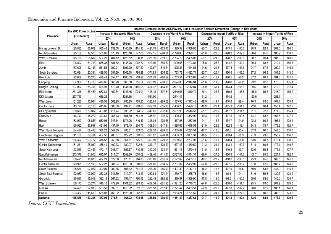
Economics and Finance Indonesia, Vol. 52, No.3, pp.335-364
29
Urban Rural Urban Rural Urban Rural Urban Rural Urban Rural Urban Rural Urban Rural Urban Rural Urban Rural
Nanggroe Aceh D. 195,882 166,608 565.46 532.08 1140.89 1101.13 -421.78 -423.45 -1989.39 -1969.86 -25.7 -28.3 -143.5 -145.3 98.9 92.1 209.0 198.0
North Sumatera 175,152 117,578 505.62 375.49 1020.16 777.08 -377.15 -298.84 -1778.86 -1390.16 -23.0 -20.0 -128.3 -102.6 88.4 65.0 186.9 139.7
West Sumatera 175,730 125,602 507.29 401.12 1023.52 830.11 -378.39 -319.23 -1784.73 -1485.03 -23.1 -21.3 -128.7 -109.6 88.7 69.4 187.5 149.3
Riau 196,892 151,718 568.38 484.52 1146.78 1002.72 -423.96 -385.60 -1999.65 -1793.81 -25.8 -25.8 -144.2 -132.3 99.4 83.8 210.1 180.3
Jambi 187,608 122,185 541.58 390.21 1092.70 807.53 -403.97 -310.54 -1905.36 -1444.63 -24.6 -20.8 -137.4 -106.6 94.7 67.5 200.2 145.2
South Sumatera 172,684 120,331 498.50 384.29 1005.78 795.28 -371.83 -305.83 -1753.79 -1422.71 -22.7 -20.4 -126.5 -105.0 87.2 66.5 184.3 143.0
Bengkulu 172,659 110,275 498.43 352.17 1005.63 728.82 -371.78 -280.27 -1753.54 -1303.82 -22.7 -18.7 -126.5 -96.2 87.2 60.9 184.3 131.0
Lampung 164,909 113,728 476.05 363.20 960.50 751.64 -355.09 -289.05 -1674.83 -1344.64 -21.6 -19.3 -120.8 -99.2 83.2 62.8 176.0 135.1
Bangka Belitung 197,082 178,701 568.93 570.70 1147.88 1181.05 -424.37 -454.18 -2001.58 -2112.84 -25.9 -30.4 -144.4 -155.9 99.5 98.8 210.3 212.4
Riau Island 231,346 156,453 667.84 499.64 1347.45 1034.01 -498.15 -397.64 -2349.57 -1849.79 -30.4 -26.6 -169.5 -136.5 116.8 86.5 246.9 185.9
DKI Jakarta 237,735 - 686.28 - 1384.66 - -511.90 - -2414.45 - -31.2 - -174.2 - 120.0 - 253.7 -
West Java 151,235 113,964 436.58 363.95 880.85 753.20 -325.65 -289.65 -1535.95 -1347.43 -19.9 -19.4 -110.8 -99.4 76.3 63.0 161.4 135.4
Central Java 143,776 120,115 415.05 383.60 837.41 793.85 -309.59 -305.28 -1460.20 -1420.16 -18.9 -20.4 -105.3 -104.8 72.6 66.4 153.4 142.7
DI Yogyakarta 160,690 130,807 463.87 417.74 935.92 864.52 -346.01 -332.46 -1631.98 -1546.57 -21.1 -22.2 -117.7 -114.1 81.1 72.3 171.5 155.4
East Java 146,743 115,272 423.61 368.13 854.69 761.84 -315.97 -292.97 -1490.33 -1362.90 -19.3 -19.6 -107.5 -100.5 74.1 63.7 156.6 137.0
Banten 183,927 108,855 530.95 347.64 1071.26 719.43 -396.04 -276.66 -1867.98 -1287.03 -24.1 -18.5 -134.7 -94.9 92.8 60.2 196.3 129.4
Bali 166,962 136,897 481.98 437.19 972.45 904.76 -359.51 -347.94 -1695.68 -1618.58 -21.9 -23.3 -122.3 -119.4 84.3 75.7 178.2 162.7
West Nusa Tenggara 134,488 109,403 388.23 349.39 783.31 723.05 -289.59 -278.06 -1365.87 -1293.51 -17.7 -18.6 -98.5 -95.4 67.9 60.5 143.5 130.0
East Nusa Tenggara 141,168 89,764 407.52 286.67 822.22 593.26 -303.97 -228.14 -1433.71 -1061.31 -18.5 -15.3 -103.4 -78.3 71.3 49.6 150.7 106.7
West Kalimantan 164,397 109,777 474.57 350.58 957.51 725.53 -353.99 -279.01 -1669.63 -1297.93 -21.6 -18.7 -120.4 -95.8 83.0 60.7 175.4 130.5
Central Kalimantan 161,231 125,980 465.44 402.33 939.07 832.61 -347.17 -320.19 -1637.47 -1489.50 -21.2 -21.4 -118.1 -109.9 81.4 69.6 172.1 149.7
South Kalimantan 163,565 107,455 472.17 343.17 952.67 710.18 -352.20 -273.11 -1661.18 -1270.48 -21.5 -18.3 -119.8 -93.7 82.6 59.4 174.6 127.7
East Kalimantan 213,378 161,910 615.97 517.07 1242.80 1070.08 -459.46 -411.51 -2167.08 -1914.31 -28.0 -27.5 -156.3 -141.2 107.7 89.5 227.7 192.4
North Sulawesi 150,421 118,675 434.23 379.00 876.11 784.33 -323.89 -301.62 -1527.69 -1403.13 -19.7 -20.2 -110.2 -103.5 75.9 65.6 160.5 141.0
Central Sulawesi 173,991 121,193 502.27 387.04 1013.39 800.98 -374.65 -308.02 -1767.07 -1432.90 -22.8 -20.6 -127.5 -105.7 87.8 67.0 185.7 144.0
South Sulawesi 138,576 97,027 400.04 309.86 807.12 641.26 -298.39 -246.60 -1407.39 -1147.18 -18.2 -16.5 -101.5 -84.6 69.9 53.6 147.9 115.3
South East Sulawesi 122,067 107,902 352.38 344.59 710.97 713.13 -262.84 -274.24 -1239.72 -1275.76 -16.0 -18.3 -89.4 -94.1 61.6 59.6 130.3 128.2
Gorontalo 135,837 115,018 392.13 367.32 791.17 760.16 -292.49 -292.33 -1379.57 -1359.90 -17.8 -19.5 -99.5 -100.3 68.6 63.6 145.0 136.7
West Sulawesi 189,173 150,271 546.10 479.90 1101.82 993.15 -407.34 -381.93 -1921.26 -1776.70 -24.8 -25.5 -138.6 -131.1 95.5 83.0 201.9 178.6
Maluku 174,425 122,936 503.52 392.61 1015.92 812.50 -375.58 -312.45 -1771.47 -1453.51 -22.9 -20.9 -127.8 -107.2 88.0 67.9 186.1 146.1
Papua 193,307 145,610 558.03 465.02 1125.90 962.35 -416.24 -370.08 -1963.24 -1721.59 -25.4 -24.7 -141.6 -127.0 97.6 80.5 206.3 173.0
National 165,565 117,365 477.95 374.81 964.32 775.68 -356.50 -298.29 -1681.49 -1387.64 -21.7 -19.9 -121.3 -102.4 83.6 64.9 176.7 139.5
the 2005 Poverty Line
(IDR/Month)Province60%20% 60%
Increase in Import Tariffs of Rice
20% 60% 20%
Increase in the World Rice Price Decrease in the World Rice Price
20% 60%
Decrease in Import Tariffs of Rice
Increase (Decrease) in the 2005 Poverty Line Line Under Selected Simulation (Change in IDR/Month)
Source: CGE Simulations

Economics and Finance Indonesia, Vol. 52, No.3, pp.335-364
30