volatility regime shifts in international public property ... · volatility regime shifts in...
TRANSCRIPT
IRES2014-009
IRES Working Paper Series
Volatility regime shifts in international public property markets
Qing Ye, Kim Hiang Liow
May 2014
1
Volatility regime shifts in international public property markets
This version: May 11th
, 2014
Miss Ye Qing1* and Professor Liow Kim Hiang
2*
Abstract
Prior research studies have indicated that stock market return series have very different properties
between low and high volatile market regimes. This paper examines this issue in ten developed
international public property market and assesses the state-dependent volatility characteristics
across these markets over the past two decades. The classification between low and high volatility
regimes provides an ideal platform to study the contagion effect during extreme market conditions.
We find that real estate securities returns can be better characterized and forecasted by a regime-
switching GARCH model compared to traditional models. Moreover, the volatility spillover is
significantly increased and market linkage is strengthened during market downturns across all
markets examined. Finally, portfolio analysis dependent on the market regimes shows superior
diversification profits than investing over constant correlation. Finally, we show that there is a
strong difference of real estate securities performance in terms of risk-return, volatility spillover
pattern and diversification benefit between financial tranquil and turmoil time.
1 Introduction
The fall of banking sector in the recent 2007 global financial crisis is mainly because
banks are largely exposed to real estate developers and mortgage lenders. The crisis has quickly
spread to all nations and pushed international real estate securities markets into great turmoil. This
upheaval in the global financial market has led researchers to reexamine the contagion effect of
real estate assets. Real estate securities market, as an important component of general equity
market, is experiencing high uncertainty. In some times it can have a great boom, but it can also
fall down all in a sudden. Prior literature shows that they display even higher volatility than
general stocks (Sagalyn, 1990; Kallberg, et al., 2002). However, they are much preferred by
investors as an additional diversification since real estate securities exhibit lower correlation
globally. While real estate securities provide investors exposure to broad areas of real estate, it is
* Department of Real Estate, School of Design and Environment, National University of Singapore
4 Architecture Drive, Singapore, 117566 1 Corresponding author: PhD Candidate, [email protected]
2 Professor, [email protected]

2
still less known whether they can offer constant benefits that hedge against the changing market
performance.
In this study, we explore, whether there is strong switching regime behavior over the past two
decades in ten developed international real estate securities markets. Given the frequently
occurred turbulence in the financial markets and its contagious nature, we expect that there is
significant regime change in the real estate securities market. We characterize the sample period
into two sub-periods: one with low market volatility (tranquil period) and the other with high
market volatility (turmoil period). From the results, we investigate whether international market
linkages have significant variation between the two periods.
We also study the varying degrees of interdependence and volatility spillovers among candidate
countries over time. The main goal is to compare the different pattern of volatility spillover
between low and high volatility market states. Following estimation of state-dependent
conditional volatility from regime switching model, we further apply the newly generalized
version of spillover index of Diebold and Yilmaz (2012) to the ten developed markets to study
the direction and magnitude of volatility spillover among international real estate securities
markets.
To understand how the introduction of switching regimes can help reduce the portfolio risk, we
compare the performance of a dynamic portfolio where the asset allocation is state-dependent with
the benchmark portfolio where the weightings are constant based on historical market
performance. Both portfolios are optimized in order to achieve the objective of minimum variance.
The switching regime strategy of portfolio construction tracts the state-varying nature of market
performance in terms of return, variance and correlation, which is expected to yield higher risk
reduction benefit than a constant strategy.
3
Though there has been extensive work that investigates time-varying relationship or contagion
effect among global real estate securitized markets, few of them condition it on market volatility
states, and more importantly, over an extensive period before and after the financial crisis period.
This study is the first to investigate international real estate securities market linkages under
switching regime market behavior. As suggested by Forbes and Rigobon (2002), correlation
coefficients are biased measurement of market dependence if markets become more volatile.
Therefore, this research is expected to improve the key understanding of market interdependence,
and especially contagion effect across markets during crisis period.
We apply a novel methodology to capture the occasional shifts in the volatility process of real
estate securities markets. Gray (1996) and Dueker (1997) developed a Markov regime-switching
GARCH (MRS-GARCH) model to allow the conditional volatility switching between two
GARCH processes governed by different normal distribution. This stream of Markov regime-
switching model has been popularly used in literature since they are able to well describe extreme
events that frequently hit the financial markets. To compare the performance of GARCH models
in terms of switching regime version and traditional one (single regime), we give the test of model
fit as well as forecasting outcomes in the context.
The empirical results, using ten developed real estate securities markets data, can be summarized
as follows: (a) The volatility in ten developed real estate securities markets is subject to regime
switching behavior and a regime switching GARCH model is superior to traditional GARCH
model in characterizing and forecasting the market volatility process. (b) Asian real estate
securities markets exhibit longer time visiting high volatility states than other counterparts, yet the
market returns are not significantly higher. (c) Cross-market correlation increases significantly
during high volatility states. (d) During the financial crisis period, the volatility spillover effect is
strengthened across markets, indicating strong interdependence, especially in the Asian markets.
4
(e) The portfolio risk is significantly reduced if the allocation strategy is dependent on the
switching regimes.
The paper is organized as follows: section 2 presents the literature devoted to examine properties
of real estate securities market volatility and dynamic linkages. Section 3 gives a detailed
description of MRS-GARCH methodologies. The data of real estate securities returns is discussed
in section 4, following by empirical results and discussions in section 5. Conclusions are
summarized in section 6.
2 Literature Review
2.1 Contagion effect in international financial market
Two main forces of financial market integration are broadly discussed in the literature. One is
globalization, which increases market integration gradually over time. The other is what I aim to
study: contagion, which occurs only in bad times. The phenomenon that the crisis originated in
one financial market can quickly spread to markets all over the world has drawn attention from
researchers. Forbes and Rigobon (2002) defines it as contagion when cross-market linkages
increase only after a shock to one country (or group of countries). Studying cross-market
contagion without accounting for changing market volatility is biased.
There are many empirical papers that study the contagion effect, to name a few, Bekaert, et al.
(2005) apply a two-factor model based on CAPM to stock markets globally and examine whether
there is sudden increase in correlations during periods of crises. They find significant increase of
correlation among Asian regions. However, in the end they point out that the result may fail to
capture asymmetric volatility and the potential effects it may exert on correlations during crisis.
They propose using a richer regime switching model to account for contagion effect. More
recently, Aloui, et al. (2011) employ a multivariate copula approach to examine extreme co-
5
movement of BRIC and the US markets. They find extreme co-movement in both the bearish and
bullish markets, but the degree is generally smaller in bearish markets among the BRIC pairs,
indicating lower probability of simultaneous crashes.
In the real estate finance literature, Wilson and Zurbruegg (2004) studied the period of Asian
financial crisis in 1997 and found that there is contagion effect from Thai securitized real estate
market to other Asian markets. But this result is sensitive to the sample period chosen and based
on a single event of Thai baht devaluation. Bond, et al. (2006) found that there was significant
increase of correlation among Asian real estate securitized markets during the crisis. But the
transmission of shocks is different between real estate stocks and general equity markets,
indicating significant cross-asset diversification opportunities. Liow, et al. (2009) also confirmed
the existence of contagion effect among Asian property markets during the Asian financial crisis,
though not significant. However, less attention has been paid to the contagion effect during the
more recent global financial crisis, of which the magnitude is expected to be larger and has a
wider scope of global markets. Therefore, this study is contributed to fill the literature gap in this
area.
2.2 Real Estate Securities Market Volatility and Co-movement
Ever since the work of Schwert (1989), both theoretical and empirical researches have come to
explain the time-varying stock return volatility. Many earlier studies have focused on the causes
of persistence of volatility of asset returns, pointing to the presence of both structural changes and
long memory, but have mostly conducted on developed markets (Giliberto, 1990; Asabere, et al.,
1991; Ross and Zisler, 1991; Devaney, 2001). Later work improves by exploring dynamic
properties of data at different frequency (Liow, et al., 2009; Hoesli and Reka, 2011), covering a
wider range of markets (Liow and Newell, 2012; Zhou and Gao, 2012) or conducting comparison
across different assets (Neil Myer and Webb, 1993; Glascock, et al., 2000).
6
Given the better performance of real estate securities than general stocks, they have attracted
much research attention. For example, Garvey, et al. (2001) studied inter-relationship between
real estate securities markets in Asia on a weekly basis. They found little evidence of market co-
movement in the short run, indicating diversification benefits within the Pacific-Rim region.
Kallberg, et al. (2002) studied regime shifts in Asian real estate securities and stock markets
during the 1997 Asian financial crisis. Generally they found evidence of switching regime
behavior in the summer of 1997 and spring of 1998, and there is evidence of common volatility
factors among the markets studied. Gerlach, et al. (2006) also studied the impact of Asian
financial crisis on Asian-pacific real estate markets. Their result suggests integration among these
markets, despite a common structural break around mid-1997.
This group of research does not yield uniform pattern of co-movement among the real estate
securities markets examined. One of the common problems is that the framework is not flexible
enough to allow for stationarity and persistence properties of real estate securities returns. To
distinguish between crisis and non-crisis period, the sample period is divided arbitrarily
(Chandrashekaran, 1999; Clayton and MacKinnon, 2003; Westerheide, 2006). Meanwhile, these
studies only focus on regional sectors of real estate markets but overlook the possible linkages
with international developed markets in the US and the UK, etc.
More recently, with the development of statistical tools, more researchers have adopted Markov
regime switching framework to study real estate securities returns. And the result generally shows
strong persistence and regime switching behavior in the real estate securities returns. Liow, et al.
(2005) examined shifts in returns and volatility Asian property markets and compared with the US
and the UK. Strong evidence of regime switching behavior is detected among international
securitized property markets. Liow and Zhu (2007) apply regime switching strategies in the asset
allocation model. A shortcoming of the two papers is that they only allow for regime switching
process in the mean equation of real estate securities return. More recently, Case, et al. (2012)
7
applied regime switching GARCH model to REITs, stock and bond return in the US over the
period 1972-2008. The result suggested existence of separate regimes in the conditional
expectation and variance process. The multivariate result indicated that REITs return was in synch
with stock but not with bonds. Though in their framework the cross-asset linkages were
considered, the synchronization among international real estate securities markets was overlooked.
With the trend of globalization and contagion effect across markets, the lead-lag relationship and
volatility synchronization remains important for both investors and practitioners.
3 Sample data
3.1 Sample market review
In this study, we focus on ten developed real estate securities markets across the world, including
Australia, Hong Kong, Japan, Singapore, France, Germany, Switzerland, United Kingdom,
Canada and United States. These markets account for a significantly large proportion of broader
equity markets in terms of market capitalization3 by rank. Given their relatively large size and
degree of openness, we expect that the sample markets are more influential toward other
international markets and reflect market trend of global real estate securities. The variation of
market linkages between tranquil and turmoil market state is also expected to be larger than within
emerging markets. An important reason we do not study emerging markets is that they are more
prone to be affected by frequent structural breaks due to equity market liberalization. And studies
of emerging markets are usually subject to poor data quality.
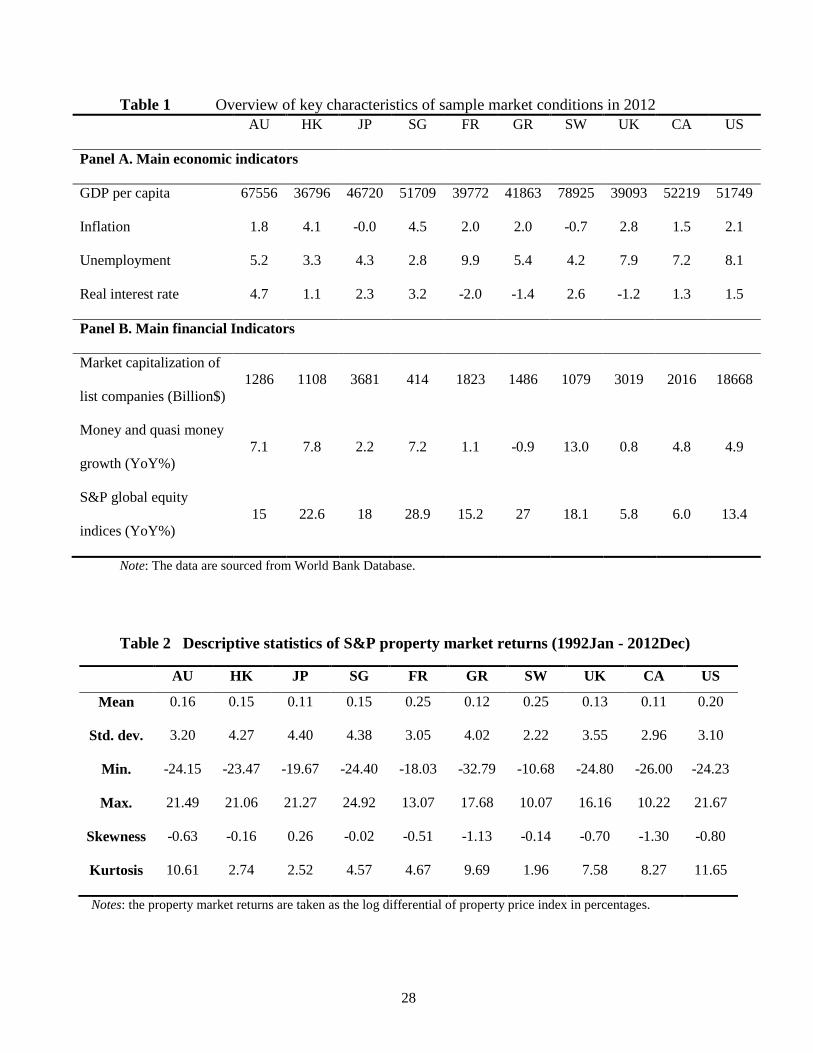
Table 1 offers a quick glimpse of the sample market conditions in the year 2012. As can be seen,
the macroeconomic conditions remain steady for most markets examined, with the exception of
European markets. And the positive return performance of the stock market also indicates the
3 Due to data availability, we exclude Brazil, Korea, Russia and India in the analysis.
8
market bounce after the financial crisis. The ten real estate securities markets studied in this
research fall into three geographical regions and different region-specific factors will play a role in
influencing their market performance.
The United States remains the top position among advanced nations in securitized property
markets. It is slowly recovering from financial turmoil due to strengthening job market and
income growth. The Canadian market, which has a close tie with the economic condition of the
US, also remained firm as the housing price is steadily showing an upward trend.
European securitized property markets are more mixed, especially after the subprime crisis. With
the support from government, the UK market is gaining traction to recover from market
downturns. And Switzerland securitized market return is seeing strong growth, benefiting from its
steady economy. Depressed labor market in Germany and France hinders these markets from
recovery, resulting in volatile performance of the securitized property markets.
While some European markets are showing weak signs, major Asian securitized property markets
are growing prosperously. It also leads to more market fluctuations in the region due to
speculation behavior. Singapore and Hong Kong’s securitized real estate markets are developing
quickly, though the Asian financial crisis in 1997 has triggered a number of large swings. With its
weak growth of the economy and the deflationary environment, Japan, the tycoon of Asian
property stock market, maintains a depressed growth compared to other Asian counterparts over
these years.
Overall, we expect the switching regime behavior to be strong in our sample markets studied.
With the occurrence of regional crisis in Asia and Europe, the volatility variation between tranquil
and turmoil period in those markets are reckoned to be larger.
[Insert Table 1 here]
9
3.2 Data description and preliminary analysis
The dataset of this study consists of weekly returns of major securitized real estate markets from
Standard and Poor (S&P) Global Database. The price indices from S&P are computed consistently
across different markets and are comparable directly. An advantage of this database is that it
covers a wide range of both emerging and developed markets for a long period at individual and
regional level. It also provides stock market index (Broader Market Index) based on the same
methodology and can be used for comparison with real estate securities index directly.
The weekly return series used in this study are computed from daily total return indices in US
dollar currency (Thursday to next Wednesday). Daily data suffer from non-synchronous trading
hours and weekend effect, while monthly data do not provide enough information. The sample
period starts from July of 1992 and ends in December of 2012, which is the longest available time
span of the database for all sample markets. There are 1069 observations in the sample.
A simple description of property return data is reported in Table 2. Over the sample period, the
Asian property market exhibits higher volatility and larger range of price variation than those of
European and North American property markets. The skewness and kurtosis statistics also
confirm the non-normality distribution of the data.
[Insert Table 2 here]
4 Methodology
In order to model the time-varying market volatility and incorporate the changes of market
performance at different market stages, we employ a switching regime GARCH model. In fact,
Hamilton and Susmel (1994) firstly introduce Markov switching model into the standard ARCH
process to overcome its poor out-of-sample forecasting ability. A Markov switching model
governs the change between different variance regimes so that in each regime, the volatility is

10
expressed by a unique ARCH process. While the variance of MS-ARCH model depends only on
the regimes of all ARCH lags, MS-GARCH model, though is more flexible and widely used, is
notoriously difficult for estimation (especially in large time-series data) since the lagged variance
term depends upon the entire history of regimes. Later, the MS-GARCH model developed by
Gray (1996) and Dueker (1997) overcome the problem by reducing the length of dependence and
approximately estimating the function. Of the two, Dueker’s filter requires only one lag of the
regime, therefore is simpler for estimation than Gray’s model. The following of this section will
start by explicitly explaining the setup of the MS-GARCH model, and describes the volatility
spillover methodology:
4.1 Switching regime GARCH model
The difference between MS-GARCH model and GARCH model is that, while GARCH model
assumes an ARMA process of volatility, the MS-GARCH model keeps same structure for
volatility, but allows the possibility of sudden jumps between two market states. It is recently
becoming popular in finance literature because it can well deal with volatility persistency and
determines the market states endogenously. A simple illustration of the model is as follows:
t t ty (1)
where ~student- t (mean=0, tn , th ) t , tn is the degree of freedom in the dependent variable ty .
The conditional mean t is allowed to switch according to a Markov process governed by a state
variable tS , indicating good time when 1tS and bad times when 0tS .
(1 )t l h tS (2)
( ) ( ) 2
1 1
1
ˆ( )( )
j j
t t t
t
h hg S j
(3)
11
where and are constant and ( 1)g S is the relative factor to scale down the ( ) 2
1( )j
t . The
initial probability of being in regime i is given by 1Pr( ) iS i p where 1S is the first regime in
the Markov chain. The transition probability between state 1 and 0 is given by:
11 12
21 22
(4)
where 1Pr( | )ij t tS j S i denotes the transition probability to state j at time t from state i
at time 1t .
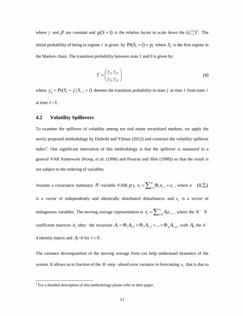
4.2 Volatility Spillovers
To examine the spillover of volatility among ten real estate securitized markets, we apply the
newly proposed methodology by Diebold and Yilmaz (2012) and construct the volatility spillover
index4. One significant innovation of this methodology is that the spillover is measured in a
general VAR framework (Koop, et al. (1996) and Pesaran and Shin (1998)) so that the result is
not subject to the ordering of variables.
Assume a covariance stationary N -variable VAR( p ), 1
p
t i t i tix x , where (0, )
is a vector of independently and identically distributed disturbances and tx is a vector of
endogenous variables. The moving average representation is 0t i t ii
x A
, where the N N´
coefficient matrices iA obey the recursion 1 1 2 2 ...i i i p i pA A A A , with 0A the 4´
4 identity matrix and iA =0 for 0i .
The variance decomposition of the moving average form can help understand dynamics of the
system. It allows us to fraction of the H -step –ahead error variance in forecasting ix that is due to
4 For a detailed description of this methodology please refer to their paper.
12
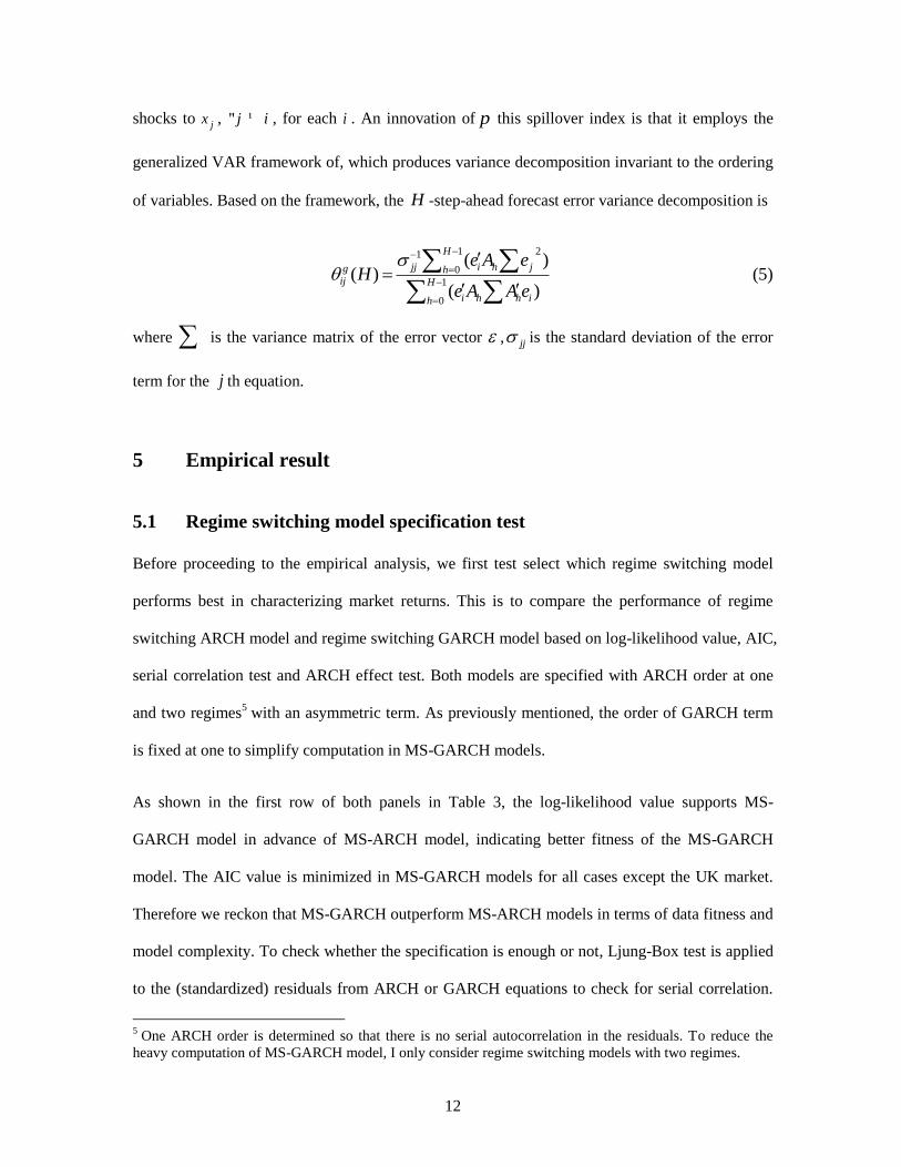
shocks to jx , j i" ¹ , for each i . An innovation of p this spillover index is that it employs the
generalized VAR framework of, which produces variance decomposition invariant to the ordering
of variables. Based on the framework, the H -step-ahead forecast error variance decomposition is
1 21
0
1
0
( )( )
( )
H
jj i h jg hij H
i h h ih
e A eH
e A A e
(5)
where is the variance matrix of the error vector , jj is the standard deviation of the error
term for the j th equation.
5 Empirical result
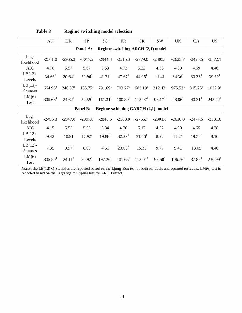
5.1 Regime switching model specification test
Before proceeding to the empirical analysis, we first test select which regime switching model
performs best in characterizing market returns. This is to compare the performance of regime
switching ARCH model and regime switching GARCH model based on log-likelihood value, AIC,
serial correlation test and ARCH effect test. Both models are specified with ARCH order at one
and two regimes5 with an asymmetric term. As previously mentioned, the order of GARCH term
is fixed at one to simplify computation in MS-GARCH models.
As shown in the first row of both panels in Table 3, the log-likelihood value supports MS-
GARCH model in advance of MS-ARCH model, indicating better fitness of the MS-GARCH
model. The AIC value is minimized in MS-GARCH models for all cases except the UK market.
Therefore we reckon that MS-GARCH outperform MS-ARCH models in terms of data fitness and
model complexity. To check whether the specification is enough or not, Ljung-Box test is applied
to the (standardized) residuals from ARCH or GARCH equations to check for serial correlation.
5 One ARCH order is determined so that there is no serial autocorrelation in the residuals. To reduce the
heavy computation of MS-GARCH model, I only consider regime switching models with two regimes.

13
For the MS-ARCH model in panel A of Table 3, the null-hypothesis is rejected for all markets
except for Switzerland at residual level, whereas for MS-GARCH model, the serial correlation is
reduced at residual levels and fully eliminated at residual squares, except for France. This is not
surprising as MS-GARCH accounts for conditional heteroskedasticity and the conditional
variance is flexible to vary across regimes. This is, however, not incorporated in the MS-ARCH
specification. Therefore, the standardized residuals are reduced to be white noise in MS-GARCH
models. The LM test in the last row of each panel also rejects the ARCH effect in the residuals.
Therefore, the result is in favor of MS-GARCH specification, where I continue the analysis
thereafter.
[Insert Table 3 here]
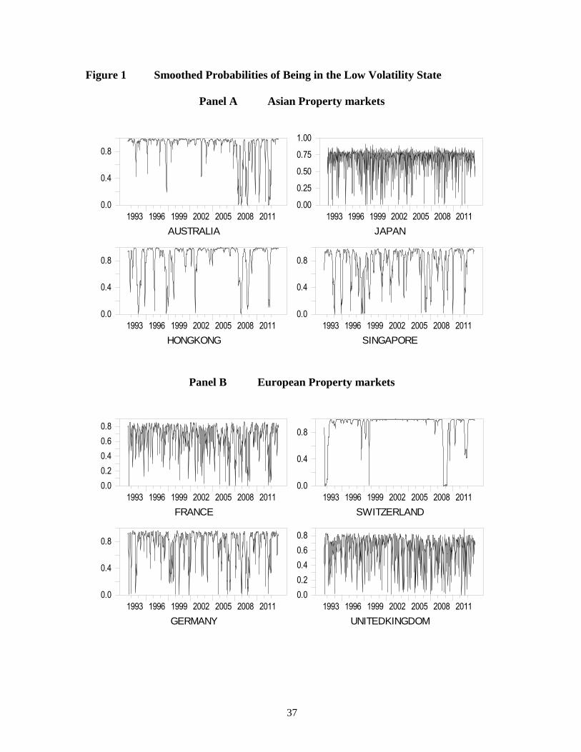
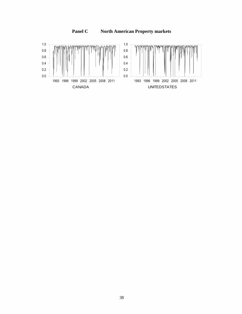
5.2 Switching regimes in international real estate securities markets
The two regimes are referred to as one low volatility regime with high return and one high
volatility regime with low return, respectively. The high volatility regime corresponds to the
financial crisis period which takes place only occasionally. The low volatility coincides with
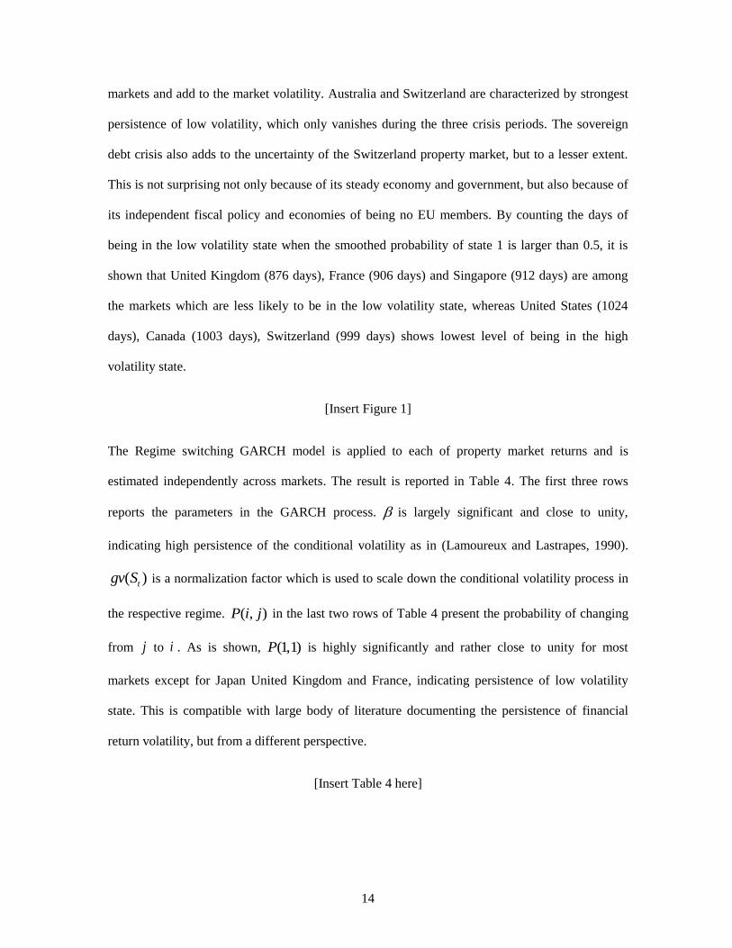
normal tranquil period and accounts for most of the sample period. Panel A to C of Figure 1 plots
the estimated probabilities of being in state 1 (low volatility state) for all the property markets
studied. We can infer the smoothed probability of being in state 2 by subtracting the plotted
probability from unity. From the result, it is observed that within Asia, the low volatility
probability of Australia property market exhibits strong persistence, whereas that of Singapore
and Japan quickly decreases to low level, which result in frequent visit of high volatility state. The
results in Panel B and C show that the probability of being in the low volatility state is less
persistent and stable , especially in Europe where the estimated probabilities are lower than unity.
The three figures also yield evidence of strong regional patterns where all markets in that region
tend to visit the particular state at the same time. The 1997 Asian financial crisis, the 2007 global
financial crisis and the following European sovereign debt crisis all influence the global property
14
markets and add to the market volatility. Australia and Switzerland are characterized by strongest
persistence of low volatility, which only vanishes during the three crisis periods. The sovereign
debt crisis also adds to the uncertainty of the Switzerland property market, but to a lesser extent.
This is not surprising not only because of its steady economy and government, but also because of
its independent fiscal policy and economies of being no EU members. By counting the days of
being in the low volatility state when the smoothed probability of state 1 is larger than 0.5, it is
shown that United Kingdom (876 days), France (906 days) and Singapore (912 days) are among
the markets which are less likely to be in the low volatility state, whereas United States (1024
days), Canada (1003 days), Switzerland (999 days) shows lowest level of being in the high
volatility state.
[Insert Figure 1]
The Regime switching GARCH model is applied to each of property market returns and is
estimated independently across markets. The result is reported in Table 4. The first three rows
reports the parameters in the GARCH process. is largely significant and close to unity,
indicating high persistence of the conditional volatility as in (Lamoureux and Lastrapes, 1990).
( )tgv S is a normalization factor which is used to scale down the conditional volatility process in
the respective regime. ( , )P i j in the last two rows of Table 4 present the probability of changing
from j to i . As is shown, (1,1)P is highly significantly and rather close to unity for most
markets except for Japan United Kingdom and France, indicating persistence of low volatility
state. This is compatible with large body of literature documenting the persistence of financial
return volatility, but from a different perspective.
[Insert Table 4 here]
15
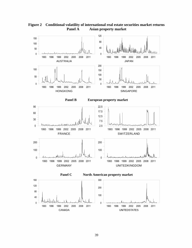
Panel A to C of Figure 2 present the time-varying conditional volatility of the sample property
market returns. Under the Markov modeling framework, the volatility process can be interpreted
as expected value since it is weighted by the normalization factor ( )tgv S in the respective state
distinguished by the smoothed probability. As is observed, the volatility persistence, which is
usually found in conventional GARCH framework, is significantly reduced. The volatility value
quickly reverts back to normal level after climbing up due to shocks. To look at the performance
of international real estate securities markets during the sample period, it is observed that the
expected variance is everywhere high during the subprime crisis around 2008, when the expected
volatility can be more than ten times higher than in normal tranquil period. For the Asian property
markets in Panel A of Figure 2, the estimated volatility reached even higher peak value during the
Asian financial crisis period, such as Hong Kong and Singapore, where the strike from the crisis is
most severe. The European property markets generally stay in the low volatility state since the
start of the sample period, but quickly climb to peak value from year 2007. After returning to
medium level, the estimated volatility in European property markets picks up again at the end of
year 2011. Particularly, it is observed that Asian property markets are more volatile than those in
Europe and North America over the sample period, especially in Japan, Hong Kong and Singapore.
Given the growing prospects of Asian markets from global real estate securities fund, it implies
that despite the higher volatility estimated, investors are still willing to allocate assets in Asian
property markets to secure higher returns.
[Insert Figure 2 here]
Table 5 presents the average return and constant variance of each real estate securities market of
two volatility states. In the terms of magnitude of variance, Japan, the US and Germany are most
volatile during high volatility state, while Switzerland and France stays quieter during crisis time.
It is also observed that Asian real estate securities markets exhibit higher volatility and spend
16
longer time in the high volatility state than other international real estate markets, yet the return is
not significantly higher during this sample period.
[Insert Table 5 here]
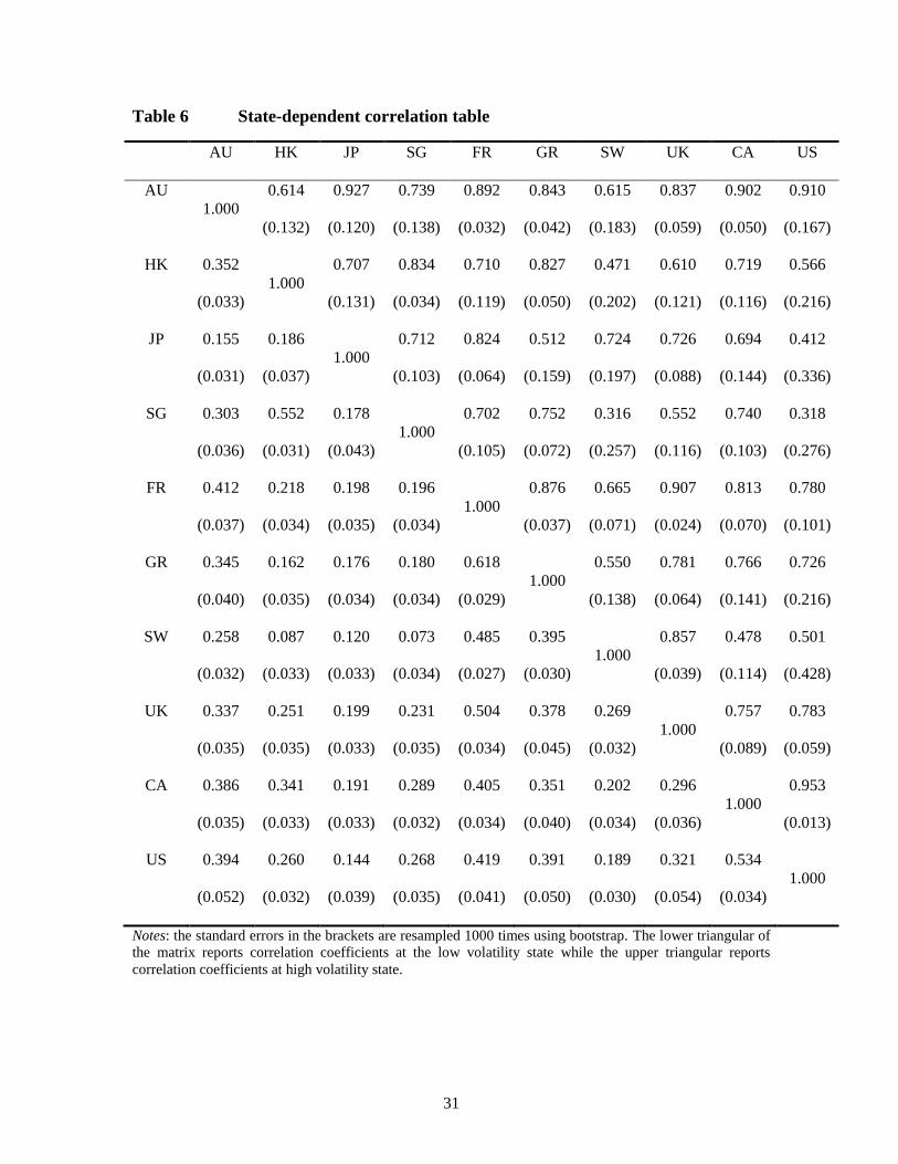
Finally, the state-dependent correlation coefficients are estimated when both markets are in the
same volatility state. Specifically, the observation belongs to low volatility state if the smoothed
probability of state one is larger than 0.5, and vice versa. The correlation coefficient in each
regime is calculated based on the series in the overlapping periods of both markets. The
correlation matrix is presented in Table 6 with the lower triangular reporting correlation
coefficients in low volatility regime and upper triangular reporting correlation coefficients in high
volatility regime. It is not surprising that the correlation coefficients are found to be much higher
for all market pairs during high volatility regime, providing evidence of contagion across markets
during crisis time.
[Insert Table 6]
From Table 5, three main regional patterns are also observed. Firstly, Singapore and Hong Kong
represent the most fast growing regions in real estate securities markets in Asia. They are also
mostly correlated during both low and high volatility regimes. Similarly, Canada and the US
exhibit highest correlation than the rest international markets in both volatility regimes. The
correlation coefficient even reaches 0.953 during high volatility period, indicating almost perfect
synchronization between the two real estate securities markets. Secondly, it appears that inter-
regional correlations increase to be the highest during high volatility period for all real estate
securities markets. This finding provides additional evidence to the work of Bekaert, et al. (2005)
that integration of regional real estate securities markets sharply increases during crisis period.
Thirdly, the increment of correlation during high volatility period in Asia is generally more than
the other counterparts, indicating that the contagious effect in bear market is higher in this region.

17
For investors, however, the findings are dangerous signals for asset allocation strategies merely at
regional levels, especially in the Asian region. Instead, based on our statistical evidence, broader
investment strategy at international levels is much recommended.
5.3 Prediction of real estate securities volatility: a comparison of MS-
GARCH and MS-ARCH models
Whilst evaluating past performance may help us understand the unique risk properties of real
estate securities, investors care more about how the introduction of regime shifts may help predict
the securities performance in the future. We next proceed to examine the one-step ahead
prediction of real estate securities conditional volatility. More importantly, we care about whether
MS-GARCH models offers better forecast ability than other regime switching models.
To conduct the out-of-sample forecast, we first estimate the one-step-ahead predictions of the
variance. In the regime switching model setting, the estimated conditional volatility is calculated
as the average of two conditional volatility processes in the low and high volatility regimes
weighted by the probabilities of the two regimes at time t given 1t . For comparison, we also
estimate and forecast regime switching ARCH(2,1)6 and GARCH (1,1) model, both with an
asymmetric term in the variance equation.
The proxy of ex-post volatility is difficult to obtain. The mean-adjusted squared return, though
unbiased, is known to be a noise measurement that leads to the bad forecasting performance of
many models (Andersen and Bollerslev, 1998). This paper follows this idea and employs the
measurement of realized volatility which can significantly reduce the noise. Since we use weekly
return and the highest frequency available is daily data, the observed volatility is calculated as the
sum of squared daily returns over a week’s horizon:
6 To be consistent, we estimate ARCH (2,1) with two volatility regimes and one lag of ARCH term.
18
52
1
t i
i
RV r
where tRV is the realized variance at week t , and ir is the daily return at trading day i .
The loss function is calculated as follows:
1 2
1 1|
1
( )n
t t t
t
MSE n RV h
1 1 1
1 1| 1|
( log 1)n
t t
t t t t t
RV RVQLIKE n
h h
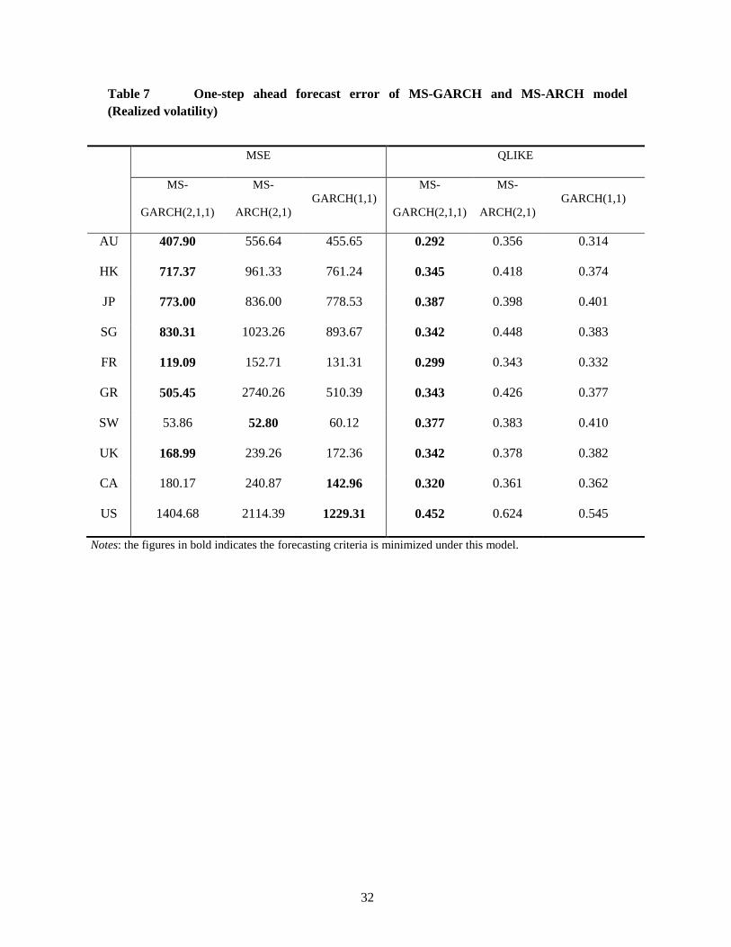
For volatility forecast comparison, Table 7 summarizes the loss function of Mean Squared Error
(MSE) and QLIKE of the one-step-ahead estimation. In terms of MSE, MS-GARCH(2,1,1) is
minimized in most markets except Switzerland, Canada and the US. But the QLIKE value
supports MS-GARCH(2,1,1) in all markets, indicating the forecasting performance gains relative
to other alternative models. The overall result supports the better performance of regime switching
models in terms of volatility forecasting, as is observed from the comparison with MS-ARCH(2,1)
and GARCH(1,1) model. This is because regime switching GARCH model is generalized to
account for the volatility persistence, which is a critical important feature of asset returns.
[Insert Table 7 here]
5.4 Volatility spillovers across markets
An important advantage of regime switching model is that it can well capture the contagion effect
during the financial crisis time. According to the definition of Forbes and Rigobon (2002),
contagion takes place only when cross-market linkages increase after a shock to one country (or
group of countries). This is usually accompanied by the increase of volatility in the financial

19
market. Regime switching model is capable to distinguish the different levels of market volatility,
which provides an unbiased measure of contagion effect (Ang and Chen, 2002).
Next I examine, in addition to contagion at return level, how volatility would spill over across real
estate securities markets during different states of market performance. Moreover, the recently-
developed method by Diebold and Yilmaz (2012) makes it possible to identify both direction and
magnitude of volatility spillover across markets.
The recent financial crisis has dramatically changed the pattern of interdependence among
international real estate securities markets and, consequently, question rises as which market
dominates the influence to other markets at regional and international level. Therefore, in this
section the aim is to explore transmission of shocks across markets and evaluate how and to what
extent the volatility of market is influenced by shocks of market within/outside the same region.
There are mainly two advantages of volatility spillover measurement employed in this paper. First,
this methodology does not require the identification or existence of crisis period, thus is less prone
to subjective problems. Secondly, the variance decomposition calculation in this method is
invariant to ordering of the variables since the underlying VAR does not depend on Cholesky
factor identification.
To implement the volatility spillover analysis, we employ the estimated conditional volatility
from MS-GARCH and measure the directional impact between any of the two markets. Before
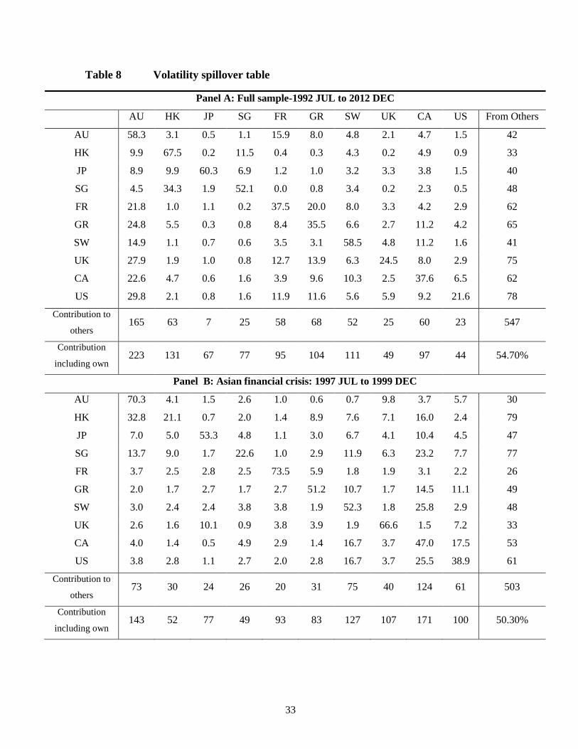
discussion, it is necessary to explain the rows and the columns of results in Table 8. The ( , )i j
element of the numerical area in the table is the estimated contribution from innovations of
volatility j to the forecast error variance of volatility i . The diagonal elements measure own-
market volatility spillovers, while the off-diagonal elements capture cross-market volatility
spillovers between two markets. The column “From Others” and row “Contribution to others”
give the total “from” and “to” volatility spillovers of each market by summing up all non-diagonal
20
elements in each row and column, respectively. The net volatility spillover from market i to
market j is calculated as the difference between the “Contribution to others” and “From Others”
in the respective market. The total volatility spillover index, given in the lower right corner of the
table, estimates the sum of the second last row “Contribution to others” over the sum of the last
row “Contribution including own”.
There are several interesting observations from Table 8. Firstly, the volatility spillovers from the
own market explains most of forecast error volatility, as shown the higher value of diagonal
elements compared with off-diagonal ones. Secondly, from panel B and C of crisis periods, the
volatility spillover from other markets increases significantly. In particular, during AFC period,
Asian real estate securities markets are more vulnerable to volatilities from other markets,
especially for the case of Hong Kong and Singapore. But other European and North American
markets are not significantly influenced. Meanwhile, in the GFC time, all sample markets exert
higher influence to others and receive more shocks, indicating strong interdependence among
these markets. Hong Kong becomes the main source of “volatility exporter” to other markets.
Thirdly, the volatility spillover has been mainly concentrated at regional level, whereas in the
crisis period, volatility transmission across regions is strengthened.
[Insert Table 8]
5.5 Portfolio diversification analysis under switching regimes
To further analyze if portfolio investment strategies can be improved by incorporating the regime-
switching framework, we construct portfolio real estate securities assets whose performance are
benchmarked by market indices. To simplify the analysis, we stay in a bivariate formulation of the
US real estate securities index and the rest individual market index. Specifically, investors in the
respective property market are assumed to diversify their portfolio risk by allocating part of their
wealth in the US real estate securities market and the rest in their domestic market. This
21
hypothesis of keeping US real estate in the portfolio is plausible as many historical and forward-
looking analyses suggest that in an optimized global portfolio, at least one-third of real estate
allocations should be invested in the US real estate7.
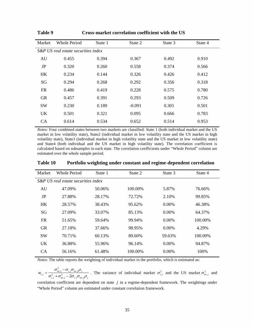
To perform this investment strategy under regime-switching framework, we classify the
performance of the two market indices into four combined states based on the smoothed
probabilities of the two markets: (a) State 1 indicates both markets are jointly in the low volatility
states; (b) State 2 is when the individual market is in the low volatility state and the US market is
in the high volatility state; (c) State 3 corresponds to the period that the individual market is in the
high volatility state and the US market in the low volatility state; (d) State 4 is the nightmare
period when both markets are in the high volatility state. The classification of four combined
states enables us to estimate the state-dependent correlation in Table 9, where we start the
portfolio analysis afterwards.
[Insert Table 9]
To construct the portfolio, it is assumed that investors are allowed to choose the proportion of the
two assets in order to minimize the portfolio risk. The formula of the portfolio variance is given
by:
2 2 2 2
, , , , , , , , ,2i j i j i j us j us j i j us j i j us j jVar w w w w (6)
where i, jw and ,us jw indicates the weighting of the individual market i and the US market in state
j and , , 1i j us jw w . 2
,i j and2
,us j is the variance of the respective market returns and j is
the state-dependent correlation between the two markets.
To achieve the objective of minimum portfolio variance, ,i jVar is derived with respect to 1, jw :
7 Source: http://www.reit.com/investing/reit-basics/reit-faqs/global-real-estate-investment
22
,
,
0i j
i j
dVar
dw (7)
and the optimal weighting of the i -th individual market is given by:
2
, , ,
, 2 2
, , , ,2
us j i j us j j
i j
i j us j i j us j j
w
(8)
The weighting ,i jw of the individual market i is reported in Table 10. As shown in the table, in
different state combinations, the weighting is significantly different from each other. For example,
in state 2 when the US market is highly volatile and the individual market is in the boom period, it
is beneficial to transfer part of the investment from the US market to the individual market. As is
shown in Table 10, compared to the normal state 1 period, the weighting of the individual market
is largely increased to almost 100% in most of the markets in state 2. Likewise, in state 3 when the
US market is tranquil and the individual market is highly volatile, the allocation of the latter is
nearly zero with the exception of Switzerland where the financial market is stable and less risky.
[Insert Table 10]
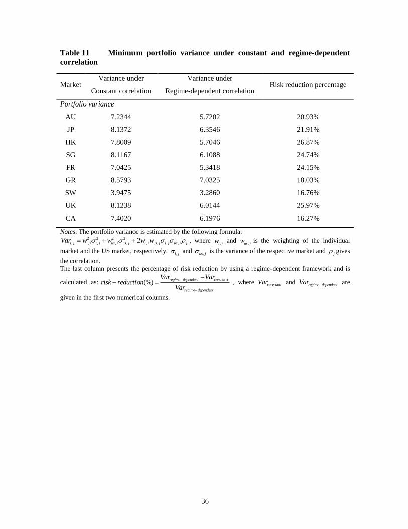
Finally, the minimized variance and risk-reduction percentage is presented in Table 11. The first
column reports the variance of the portfolio without taking a regime switching strategy, while the
last two columns report the portfolio variance under regime switching and its risk reduction
percentage. As can be seen, the portfolio risk can be significantly reduced by around 20% in all
markets if the regime-dependent correlation is considered. It offers important implications for
investors to diversify part of their assets to a less-correlated or tranquil market when the domestic
market is highly risky. This state-dependent investment strategy will significantly reduce their
portfolio risk than a constant allocation strategy.
[Insert Table 11]
23
6 Conclusion
The dynamic correlation and volatility of international real estate securities markets have been
well studied. Motivated by the frequent occurrence of extreme financial events and persistence of
shocks, this study provides a different perspective by distinguishing between low and high
volatility period where the pattern of interdependence and contagion effect across markets could
be dramatically different. The fruitful result produced provides a number of valuable additions to
the existing literature: (a) There exists significant regime switching behavior between low and
high volatility period among the sample real estate securities markets. (b) The GARCH model
with switching regimes in the conditional volatility process can well deal with the volatility
persistence issues usually found in previous literature. (c) Asian real estate securities markets,
especially Hong Kong and Singapore, exhibit higher level and persistence of volatility than
European and North American counterparts. (d) The regime switching GARCH model performs
better in terms of forecasting ability than GARCH model or regime switching ARCH model for
the sample markets studied. (e) Correlation and volatility spillover among real estate securities
markets still remain at regional levels, whereas during the crisis time, the pattern of international
interdependence is much strengthened. (f) The portfolio analysis shows strong diversification
benefits if the allocation of assets is dependent on the switching regimes. Compared to the strategy
of making investment constantly over the whole period, the switching regime method can lower
the portfolio risk by around 20% for all sample markets.
Based on the regime switching model in this paper, the result is closely associated with literature
concerns the integration and contagion of international real estate securities markets and portfolio
risk management. Future research can explore the macroeconomic factors that drive the switching
regime behavior of real estate securities market returns and dynamic correlations. Expansions of
wider sample markets that include emerging markets may provide additional evidence on the

24
volatility and correlation dynamics of real estate securities markets and is a promising area for
future work.
25
Reference
Aloui, R., Aïssa, M.S.B., Nguyen, D.K., 2011. Global financial crisis, extreme interdependences,
and contagion effects: The role of economic structure? Journal of Banking & Finance 35, 130-141
Andersen, T.G., Bollerslev, T., 1998. Answering the skeptics: Yes, standard volatility models do
provide accurate forecasts. International economic review, 885-905
Ang, A., Chen, J., 2002. Asymmetric correlations of equity portfolios. Journal of Financial
Economics 63, 443-494
Asabere, P.K., Kleiman, R., McGowan, C., 1991. The Risk-Return Attributes of International
Real Estate Equities. Journal of Real Estate Research
Bekaert, G., Harvey, C.R., Ng, A., 2005. Market Integration and Contagion. The Journal of
Business 78, 39-69
Bond, S.A., Dungey, M., Fry, R., 2006. A web of shocks: crises across Asian real estate markets.
The Journal of Real Estate Finance and Economics 32, 253-274
Case, B., Guidolin, M., Yildrim, Y., 2012. Markov Switching Dynamics in REIT Returns:
Univariate and Multivariate Evidence. Real Estate Economics, Forthcoming
Chandrashekaran, V., 1999. Time-series properties and diversification benefits of REIT returns.
Journal of Real Estate Research 17, 91-112
Clayton, J., MacKinnon, G., 2003. The Relative Importance of Stock, Bond and Real Estate
Factors in Explaining REIT Returns. The Journal of Real Estate Finance and Economics 27, 39-60
Devaney, M., 2001. Time varying risk premia for real estate investment trusts: A GARCH-M
model. The Quarterly Review of Economics and Finance 41, 335-346
Diebold, F.X., Yilmaz, K., 2012. Better to give than to receive: Predictive directional
measurement of volatility spillovers. International Journal of Forecasting 28, 57-66
Dueker, M.J., 1997. Markov switching in GARCH processes and mean-reverting stock-market
volatility. Journal of Business & Economic Statistics 15, 26-34
26
Forbes, K.J., Rigobon, R., 2002. No contagion, only interdependence: measuring stock market
comovements. The Journal of Finance 57, 2223-2261
Garvey, R., Santry, G., Stevenson, S., 2001. The linkages between real estate securities in the
Asia-Pacific. Pacific Rim Property Research Journal 7, 240-258
Gerlach, R., Wilson, P., Zurbruegg, R., 2006. Structural breaks and diversification: the impact of
the 1997 Asian financial crisis on the integration of Asia-Pacific real estate markets. Journal of
International Money and Finance 25, 974-991
Giliberto, M.S., 1990. Equity real estate investment trusts and real estate returns. Journal of Real
Estate Research 5, 259-263
Glascock, J.L., Lu, C., So, R.W., 2000. Further evidence on the integration of REIT, bond, and
stock returns. The Journal of Real Estate Finance and Economics 20, 177-194
Gray, S.F., 1996. Modeling the conditional distribution of interest rates as a regime-switching
process. Journal of Financial Economics 42, 27-62
Hamilton, J.D., Susmel, R., 1994. Autoregressive conditional heteroskedasticity and changes in
regime. Journal of Econometrics 64, 307-333
Hoesli, M., Reka, K., 2011. Volatility spillovers, comovements and contagion in securitized real
estate markets. The Journal of Real Estate Finance and Economics, 1-35
Kallberg, J.G., Liu, C.H., Pasquariello, P., 2002. Regime shifts in Asian equity and real estate
markets. Real Estate Economics 30, 263-291
Koop, G., Pesaran, M.H., Potter, S.M., 1996. Impulse response analysis in nonlinear multivariate
models. Journal of Econometrics 74, 119-147
Lamoureux, C.G., Lastrapes, W.D., 1990. Persistence in variance, structural change, and the
GARCH model. Journal of Business & Economic Statistics, 225-234
Liow, K., Zhu, H., 2007. Regime switching and asset allocation: Evidence from international real
estate security markets. Journal of Property Investment & Finance 25, 274-288

27
Liow, K.H., Ho, K.H.D., Ibrahim, M.F., Chen, Z., 2009. Correlation and volatility dynamics in
international real estate securities markets. The Journal of Real Estate Finance and Economics 39,
202-223
Liow, K.H., Newell, G., 2012. Investment dynamics of the Greater China securitized real estate
markets. Journal of Real Estate Research 34, 399-428
Liow, K.H., Zhu, H., Ho, D.K., Addae-Dapaah, K., 2005. Regime changes in international
securitized property markets. Journal of Real Estate Portfolio Management 11, 147-165
Neil Myer, F., Webb, J.R., 1993. Return properties of equity REITs, common stocks, and
commercial real estate: a comparison. Journal of Real Estate Research 8, 87-106
Pesaran, H.H., Shin, Y., 1998. Generalized impulse response analysis in linear multivariate
models. Economics letters 58, 17-29
Ross, S.A., Zisler, R.C., 1991. Risk and return in real estate. The Journal of Real Estate Finance
and Economics 4, 175-190
Sagalyn, L.B., 1990. Real estate risk and the business cycle: evidence from security markets.
Journal of Real Estate Research 5, 203-219
Schwert, G.W., 1989. Why Does Stock Market Volatility Change over Time? Journal of Finance
44, 1115-53
Westerheide, P., 2006. Cointegration of real estate stocks and REITs with common stocks, bonds
and consumer price inflation-An international comparison. ZEW-Centre for European Economic
Research Discussion Paper
Wilson, P., Zurbruegg, R., 2004. Contagion or interdependence?: Evidence from comovements in
Asia-Pacific securitised real estate markets during the 1997 crisis. Journal of Property Investment
& Finance 22, 401-413
Zhou, J., Gao, Y., 2012. Tail dependence in international real estate securities markets. The
Journal of Real Estate Finance and Economics 45, 128-151
28
Table 1 Overview of key characteristics of sample market conditions in 2012
AU HK JP SG FR GR SW UK CA US
Panel A. Main economic indicators
GDP per capita 67556 36796 46720 51709 39772 41863 78925 39093 52219 51749
Inflation 1.8 4.1 -0.0 4.5 2.0 2.0 -0.7 2.8 1.5 2.1
Unemployment 5.2 3.3 4.3 2.8 9.9 5.4 4.2 7.9 7.2 8.1
Real interest rate 4.7 1.1 2.3 3.2 -2.0 -1.4 2.6 -1.2 1.3 1.5
Panel B. Main financial Indicators
Market capitalization of
list companies (Billion$)
1286 1108 3681 414 1823 1486 1079 3019 2016 18668
Money and quasi money
growth (YoY%)
7.1 7.8 2.2 7.2 1.1 -0.9 13.0 0.8 4.8 4.9
S&P global equity
indices (YoY%)
15 22.6 18 28.9 15.2 27 18.1 5.8 6.0 13.4
Note: The data are sourced from World Bank Database.
Table 2 Descriptive statistics of S&P property market returns (1992Jan - 2012Dec)
AU HK JP SG FR GR SW UK CA US
Mean 0.16 0.15 0.11 0.15 0.25 0.12 0.25 0.13 0.11 0.20
Std. dev. 3.20 4.27 4.40 4.38 3.05 4.02 2.22 3.55 2.96 3.10
Min. -24.15 -23.47 -19.67 -24.40 -18.03 -32.79 -10.68 -24.80 -26.00 -24.23
Max. 21.49 21.06 21.27 24.92 13.07 17.68 10.07 16.16 10.22 21.67
Skewness -0.63 -0.16 0.26 -0.02 -0.51 -1.13 -0.14 -0.70 -1.30 -0.80
Kurtosis 10.61 2.74 2.52 4.57 4.67 9.69 1.96 7.58 8.27 11.65
Notes: the property market returns are taken as the log differential of property price index in percentages.
29
Table 3 Regime switching model selection
AU HK JP SG FR GR SW UK CA US
Panel A: Regime switching ARCH (2,1) model
Log-
likelihood -2501.0 -2965.3 -3017.2 -2944.3 -2515.3 -2779.0 -2303.8 -2623.7 -2495.5 -2372.1
AIC 4.70 5.57 5.67 5.53 4.73 5.22 4.33 4.89 4.69 4.46
LB(12)-
Levels 34.66
1 20.64
2 29.96
1 41.31
1 47.67
1 44.05
1 11.41
34.36
1 30.33
1 39.69
1
LB(12)-
Squares 664.96
1 246.87
1 135.75
1 791.69
1 703.27
1 683.19
1 212.42
1 975.52
1 345.25
1 1032.9
1
LM(6)
Test 305.66
1 24.62
1 52.59
1 161.31
1 100.89
1 113.97
1 98.17
1 98.86
1 40.31
1 243.42
1
Panel B: Regime switching GARCH (2,1) model
Log-
likelihood -2495.3 -2947.0 -2997.8 -2846.6 -2503.0 -2755.7 -2301.6 -2610.0 -2474.5 -2331.6
AIC 4.15 5.53 5.63 5.34 4.70 5.17 4.32 4.90 4.65 4.38
LB(12)-
Levels 9.42 10.91 17.92
2 19.88
1 32.29
1 31.66
1 8.22 17.21 19.58
3 8.10
LB(12)-
Squares 7.35 9.97 8.00
4.61
23.03
2 15.35 9.77 9.41 13.05 4.46
LM(6)
Test 305.50
1 24.11
1 50.92
1 192.26
1 101.65
1 113.01
1 97.60
1 106.76
1 37.82
1 230.99
1
Notes: the LB(12) Q-Statistics are reported based on the Ljung-Box test of both residuals and squared residuals. LM(6) test is
reported based on the Lagrange multiplier test for ARCH effect.

30
Table 4 Regime switching GARCH model result
AU HK JP SG FR GR SW UK CA US
-0.013
(0.023)
0.034
(0.021)
0.0221
(0.001)
0.0641
(0.020)
0.0422
(0.017)
0.0781
(0.025)
0.0323
(0.018)
0.0662
(0.031)
0.029
(0.029)
0.0962
(0.040)
0.9362
(0.022)
0.9211
(0.020)
0.8881
(0.006)
0.8961
(0.020)
0.9411
(0.017)
0.9021
(0.028)
0.9241
(0.010)
0.8251
(0.040)
0.8691
(0.043)
0.8561
(0.046)
0.1132
(0.024)
0.0582
(0.029)
0.1181
(0.003)
0.0552
(0.024)
0.027
(0.017)
0.023
(0.025)
-0.003
(0.016)
0.1251
(0.040)
0.1271
(0.036)
0.0822
(0.041)
0.1011
(0.031)
0.1922
(0.080)
0.3331
(0.025)
0.0912
(0.040)
0.0232
(0.010)
0.073
(0.050)
0.1641
(0.003)
0.2122
(0.089)
0.1582
(0.072)
0.047
(0.029)
0.4721
(0.166)
0.7572
(0.349)
1.1001
(0.069)
0.3672
(0.163)
0.0632
(0.028)
0.296
(0.186)
0.7351
(0.186)
0.6992
(0.272)
0.7842
(0.371)
0.287
(0.177)
P(1,1) 0.9771
(0.014)
0.9781
(0.012)
0.6481
(0.072)
0.9531
(0.025)
0.8301
(0.168)
0.9191
(0.052)
0.9911
(0.007)
0.7571
(0.093)
0.9391
(0.035)
0.9381
(0.029)
P(1,2) 0.1683
(0.096)
0.134
(0.087)
0.7831
(0.191)
0.1702
(0.079)
0.3432
(0.147)
0.2842
(0.122)
0.0912
(0.044)
0.4352
(0.034)
0.3882
(0.181)
0.5271
(0.185)
Notes: results are reported based on the equation: 1
2 2
, 1 , 1
, , 1 { 0}1( ) ( )
t t
t t t
s t s t
s t s t uR
t t
u uh h
gv s gv s
.
Table 5 Return and variance in two volatility states: 1992 Jul to 2012 Dec
AU HK JP SG FR GR SW UK CA US
Panel A: Low volatility state
Mean 0.31 0.28 0.15 0.28 0.37 0.20 0.30 0.26 0.32 0.32
Variance 5.69 12.21 9.52 11.00 4.70 8.03 3.66 4.27 5.19 6.61
# of Obs 982 952 945 912 906 931 999 876 1003 1024
Panel B: High volatility state
Mean. -0.13 -0.10 -0.02 -0.10 -0.08 -0.06 -0.02 -0.09 -0.20 -0.11
Variance 61.33 67.83 96.48 67.35 35.06 72.91 23.65 50.73 55.14 76.34
# of Obs 84 114 121 154 160 135 67 190 63 42
31
Table 6 State-dependent correlation table
AU HK JP SG FR GR SW UK CA US
AU
1.000
0.614
(0.132)
0.927
(0.120)
0.739
(0.138)
0.892
(0.032)
0.843
(0.042)
0.615
(0.183)
0.837
(0.059)
0.902
(0.050)
0.910
(0.167)
HK 0.352
(0.033)
1.000
0.707
(0.131)
0.834
(0.034)
0.710
(0.119)
0.827
(0.050)
0.471
(0.202)
0.610
(0.121)
0.719
(0.116)
0.566
(0.216)
JP 0.155
(0.031)
0.186
(0.037)
1.000
0.712
(0.103)
0.824
(0.064)
0.512
(0.159)
0.724
(0.197)
0.726
(0.088)
0.694
(0.144)
0.412
(0.336)
SG 0.303
(0.036)
0.552
(0.031)
0.178
(0.043)
1.000
0.702
(0.105)
0.752
(0.072)
0.316
(0.257)
0.552
(0.116)
0.740
(0.103)
0.318
(0.276)
FR 0.412
(0.037)
0.218
(0.034)
0.198
(0.035)
0.196
(0.034)
1.000
0.876
(0.037)
0.665
(0.071)
0.907
(0.024)
0.813
(0.070)
0.780
(0.101)
GR 0.345
(0.040)
0.162
(0.035)
0.176
(0.034)
0.180
(0.034)
0.618
(0.029)
1.000
0.550
(0.138)
0.781
(0.064)
0.766
(0.141)
0.726
(0.216)
SW 0.258
(0.032)
0.087
(0.033)
0.120
(0.033)
0.073
(0.034)
0.485
(0.027)
0.395
(0.030)
1.000
0.857
(0.039)
0.478
(0.114)
0.501
(0.428)
UK 0.337
(0.035)
0.251
(0.035)
0.199
(0.033)
0.231
(0.035)
0.504
(0.034)
0.378
(0.045)
0.269
(0.032)
1.000
0.757
(0.089)
0.783
(0.059)
CA 0.386
(0.035)
0.341
(0.033)
0.191
(0.033)
0.289
(0.032)
0.405
(0.034)
0.351
(0.040)
0.202
(0.034)
0.296
(0.036)
1.000
0.953
(0.013)
US 0.394
(0.052)
0.260
(0.032)
0.144
(0.039)
0.268
(0.035)
0.419
(0.041)
0.391
(0.050)
0.189
(0.030)
0.321
(0.054)
0.534
(0.034)
1.000
Notes: the standard errors in the brackets are resampled 1000 times using bootstrap. The lower triangular of
the matrix reports correlation coefficients at the low volatility state while the upper triangular reports
correlation coefficients at high volatility state.
32
Table 7 One-step ahead forecast error of MS-GARCH and MS-ARCH model
(Realized volatility)
Notes: the figures in bold indicates the forecasting criteria is minimized under this model.
MSE QLIKE
MS-
GARCH(2,1,1)
MS-
ARCH(2,1)
GARCH(1,1)
MS-
GARCH(2,1,1)
MS-
ARCH(2,1)
GARCH(1,1)
AU 407.90 556.64 455.65 0.292 0.356 0.314
HK 717.37 961.33 761.24 0.345 0.418 0.374
JP 773.00 836.00 778.53 0.387 0.398 0.401
SG 830.31 1023.26 893.67 0.342 0.448 0.383
FR 119.09 152.71 131.31 0.299 0.343 0.332
GR 505.45 2740.26 510.39 0.343 0.426 0.377
SW 53.86 52.80 60.12 0.377 0.383 0.410
UK 168.99 239.26 172.36 0.342 0.378 0.382
CA 180.17 240.87 142.96 0.320 0.361 0.362
US 1404.68 2114.39 1229.31 0.452 0.624 0.545
33
Table 8 Volatility spillover table
Panel A: Full sample-1992 JUL to 2012 DEC
AU HK JP SG FR GR SW UK CA US From Others
AU 58.3 3.1 0.5 1.1 15.9 8.0 4.8 2.1 4.7 1.5 42
HK 9.9 67.5 0.2 11.5 0.4 0.3 4.3 0.2 4.9 0.9 33
JP 8.9 9.9 60.3 6.9 1.2 1.0 3.2 3.3 3.8 1.5 40
SG 4.5 34.3 1.9 52.1 0.0 0.8 3.4 0.2 2.3 0.5 48
FR 21.8 1.0 1.1 0.2 37.5 20.0 8.0 3.3 4.2 2.9 62
GR 24.8 5.5 0.3 0.8 8.4 35.5 6.6 2.7 11.2 4.2 65
SW 14.9 1.1 0.7 0.6 3.5 3.1 58.5 4.8 11.2 1.6 41
UK 27.9 1.9 1.0 0.8 12.7 13.9 6.3 24.5 8.0 2.9 75
CA 22.6 4.7 0.6 1.6 3.9 9.6 10.3 2.5 37.6 6.5 62
US 29.8 2.1 0.8 1.6 11.9 11.6 5.6 5.9 9.2 21.6 78
Contribution to
others 165 63 7 25 58 68 52 25 60 23 547
Contribution
including own 223 131 67 77 95 104 111 49 97 44 54.70%
Panel B: Asian financial crisis: 1997 JUL to 1999 DEC
AU 70.3 4.1 1.5 2.6 1.0 0.6 0.7 9.8 3.7 5.7 30
HK 32.8 21.1 0.7 2.0 1.4 8.9 7.6 7.1 16.0 2.4 79
JP 7.0 5.0 53.3 4.8 1.1 3.0 6.7 4.1 10.4 4.5 47
SG 13.7 9.0 1.7 22.6 1.0 2.9 11.9 6.3 23.2 7.7 77
FR 3.7 2.5 2.8 2.5 73.5 5.9 1.8 1.9 3.1 2.2 26
GR 2.0 1.7 2.7 1.7 2.7 51.2 10.7 1.7 14.5 11.1 49
SW 3.0 2.4 2.4 3.8 3.8 1.9 52.3 1.8 25.8 2.9 48
UK 2.6 1.6 10.1 0.9 3.8 3.9 1.9 66.6 1.5 7.2 33
CA 4.0 1.4 0.5 4.9 2.9 1.4 16.7 3.7 47.0 17.5 53
US 3.8 2.8 1.1 2.7 2.0 2.8 16.7 3.7 25.5 38.9 61
Contribution to
others 73 30 24 26 20 31 75 40 124 61 503
Contribution
including own 143 52 77 49 93 83 127 107 171 100 50.30%

34
Panel C Global financial crisis: 2007 JUL to 2009 DEC
AU 23.2 25.2 3.5 10.1 7.8 6.4 13.1 3.0 2.6 5.0 77
HK 12.7 41.3 3.5 7.3 7.6 4.6 11.4 2.9 2.5 6.1 59
JP 11.9 18.3 16.0 11.7 6.7 5.0 14.1 4.6 6.2 5.4 84
SG 17.9 26.3 3.5 12.5 5.9 3.3 22.2 2.3 2.1 4.0 88
FR 9.2 30.4 2.4 7.0 16.7 9.1 10.3 6.4 3.0 5.4 83
GR 8.6 42.4 1.9 4.4 9.8 6.9 14.1 2.3 2.2 7.3 93
SW 17.7 42.6 3.9 8.3 6.8 2.1 10.2 1.9 0.8 5.8 90
UK 12.0 25.0 2.3 9.4 13.2 8.9 9.8 9.4 5.0 5.1 91
CA 15.3 27.6 3.0 10.5 6.7 5.1 15.2 3.5 6.4 6.8 94
US 15.4 30.5 3.0 10.9 7.0 6.5 9.8 3.9 3.6 9.4 91
Contribution to
others 121 268 27 80 72 51 120 31 28 51 848
Contribution
including own 144 310 43 92 88 58 130 40 34 60 84.80%
Notes: results are reported based on variance decomposition for estimated VAR(3) models of the conditional volatility obtained from the
MS-GARCH model. Lag length of 3 is selected by SIC. Variance decompositions are based on 20-week-ahead forecasts.
35
Table 9 Cross-market correlation coefficient with the US
Market Whole Period State 1 State 2 State 3 State 4
S&P US real estate securities index
AU 0.455 0.394 0.367 0.492 0.910
JP 0.320 0.260 0.558 0.374 0.566
HK 0.234 0.144 0.326 0.426 0.412
SG 0.294 0.268 0.292 0.356 0.318
FR 0.486 0.419 0.228 0.575 0.780
GR 0.457 0.391 0.293 0.509 0.726
SW 0.230 0.189 -0.091 0.301 0.501
UK 0.501 0.321 0.095 0.666 0.783
CA 0.614 0.534 0.652 0.514 0.953
Notes: Four combined states between two markets are classified: State 1 (both individual market and the US
market in low volatility state), State2 (individual market in low volatility state and the US market in high
volatility state), State3 (individual market in high volatility state and the US market in low volatility state)
and State4 (both individual and the US market in high volatility state). The correlation coefficient is
calculated based on subsamples in each state. The correlation coefficients under “Whole Period” column are
estimated over the whole sample period.
Table 10 Portfolio weighting under constant and regime-dependent correlation
Market Whole Period State 1 State 2 State 3 State 4
S&P US real estate securities index
AU 47.09% 50.06% 100.00% 5.87% 76.66%
JP 27.88% 28.17% 72.72% 2.10% 99.85%
HK 28.57% 38.43% 95.62% 0.00% 46.38%
SG 27.09% 33.07% 85.13% 0.00% 64.37%
FR 51.65% 59.64% 99.94% 0.00% 100.00%
GR 27.18% 37.66% 98.95% 0.00% 4.29%
SW 70.71% 60.13% 89.60% 59.63% 100.00%
UK 36.88% 55.96% 96.14% 0.00% 94.87%
CA 56.16% 61.48% 100.00% 0.00% 100%
Notes: The table reports the weighting of individual market in the portfolio, which is estimated as:
2
, , ,
, 2 2
, , , ,2
us j i j us j j
i j
i j us j i j us j j
w
. The variance of individual market
2
,i j and the US market2
,us j and
correlation coefficient are dependent on state j in a regime-dependent framework. The weightings under
“Whole Period” column are estimated under constant correlation framework.
36
Table 11 Minimum portfolio variance under constant and regime-dependent
correlation
Market Variance under
Constant correlation
Variance under
Regime-dependent correlation Risk reduction percentage
Portfolio variance
AU 7.2344 5.7202 20.93%
JP 8.1372 6.3546 21.91%
HK 7.8009 5.7046 26.87%
SG 8.1167 6.1088 24.74%
FR 7.0425 5.3418 24.15%
GR 8.5793 7.0325 18.03%
SW 3.9475 3.2860 16.76%
UK 8.1238 6.0144 25.97%
CA 7.4020 6.1976 16.27%
Notes: The portfolio variance is estimated by the following formula: 2 2 2 2
, , , , , , , , ,2i j i j i j us j us j i j us j i j us j jVar w w w w , where ,i jw and
,us jw is the weighting of the individual
market and the US market, respectively. ,i j and
,us j is the variance of the respective market and j gives
the correlation.
The last column presents the percentage of risk reduction by using a regime-dependent framework and is
calculated as:tan
(%)regime dependent cons t
regime dependent
Var Varrisk reduction
Var
, where tancons tVar and regime dependentVar are
given in the first two numerical columns.
37
Figure 1 Smoothed Probabilities of Being in the Low Volatility State
Panel A Asian Property markets
Panel B European Property markets
AUSTRALIA
1993 1996 1999 2002 2005 2008 2011
0.0
0.4
0.8
HONGKONG
1993 1996 1999 2002 2005 2008 2011
0.0
0.4
0.8
JAPAN
1993 1996 1999 2002 2005 2008 2011
0.00
0.25
0.50
0.75
1.00
SINGAPORE
1993 1996 1999 2002 2005 2008 2011
0.0
0.4
0.8
FRANCE
1993 1996 1999 2002 2005 2008 2011
0.0
0.2
0.4
0.6
0.8
GERMANY
1993 1996 1999 2002 2005 2008 2011
0.0
0.4
0.8
SWITZERLAND
1993 1996 1999 2002 2005 2008 2011
0.0
0.4
0.8
UNITEDKINGDOM
1993 1996 1999 2002 2005 2008 2011
0.0
0.2
0.4
0.6
0.8
38
Panel C North American Property markets
CANADA
1993 1996 1999 2002 2005 2008 2011
0.0
0.2
0.4
0.6
0.8
1.0
UNITEDSTATES
1993 1996 1999 2002 2005 2008 2011
0.0
0.2
0.4
0.6
0.8
1.0
39
Figure 2 Conditional volatility of international real estate securities market returns
Panel A Asian property market
Panel B European property market
Panel C North American property market
AUSTRALIA
1993 1996 1999 2002 2005 2008 2011
0
50
100
150
HONGKONG
1993 1996 1999 2002 2005 2008 2011
0
50
100
JAPAN
1993 1996 1999 2002 2005 2008 2011
0
40
80
120
SINGAPORE
1993 1996 1999 2002 2005 2008 2011
0
50
100
150
200
FRANCE
1993 1996 1999 2002 2005 2008 2011
0
30
60
90
GERMANY
1993 1996 1999 2002 2005 2008 2011
0
100
200
SWITZERLAND
1993 1996 1999 2002 2005 2008 2011
2.5
7.5
12.5
17.5
22.5
UNITEDKINGDOM
1993 1996 1999 2002 2005 2008 2011
0
100
200
CANADA
1993 1996 1999 2002 2005 2008 2011
0
40
80
120
160
UNITEDSTATES
1993 1996 1999 2002 2005 2008 2011
0
100
200
300