volume and surface integral equations for solving forward
TRANSCRIPT

University of KentuckyUKnowledge
Theses and Dissertations--Electrical and ComputerEngineering Electrical and Computer Engineering
2014
Volume and Surface Integral Equations for SolvingForward and Inverse Scattering ProblemsXiande CaoUniversity of Kentucky, [email protected]
This Doctoral Dissertation is brought to you for free and open access by the Electrical and Computer Engineering at UKnowledge. It has been acceptedfor inclusion in Theses and Dissertations--Electrical and Computer Engineering by an authorized administrator of UKnowledge. For more information,please contact [email protected].
Recommended CitationCao, Xiande, "Volume and Surface Integral Equations for Solving Forward and Inverse Scattering Problems" (2014). Theses andDissertations--Electrical and Computer Engineering. Paper 65.http://uknowledge.uky.edu/ece_etds/65

STUDENT AGREEMENT:
I represent that my thesis or dissertation and abstract are my original work. Proper attribution has beengiven to all outside sources. I understand that I am solely responsible for obtaining any needed copyrightpermissions. I have obtained and attached hereto needed written permission statement(s) from theowner(s) of each third-party copyrighted matter to be included in my work, allowing electronicdistribution (if such use is not permitted by the fair use doctrine).
I hereby grant to The University of Kentucky and its agents the irrevocable, non-exclusive, and royalty-free license to archive and make accessible my work in whole or in part in all forms of media, now orhereafter known. I agree that the document mentioned above may be made available immediately forworldwide access unless a preapproved embargo applies. I retain all other ownership rights to thecopyright of my work. I also retain the right to use in future works (such as articles or books) all or partof my work. I understand that I am free to register the copyright to my work.
REVIEW, APPROVAL AND ACCEPTANCE
The document mentioned above has been reviewed and accepted by the student’s advisor, on behalf ofthe advisory committee, and by the Director of Graduate Studies (DGS), on behalf of the program; weverify that this is the final, approved version of the student’s dissertation including all changes requiredby the advisory committee. The undersigned agree to abide by the statements above.
Xiande Cao, Student
Dr. Cai-Cheng Lu, Major Professor
Dr. Cai-Cheng Lu, Director of Graduate Studies

Volume and Surface Integral Equations for Solving Forward and Inverse Scattering
Problems
DISSERTATION
A dissertation submitted in partial fulfillment of the requirements for the
degree of Doctor of Philosophy in the College of Engineering at the
University of Kentucky
By
Xiande Cao
Lexington, Kentucky
Director: Dr. Cai-Cheng Lu,
Professor of Electrical and Computer Engineering
Lexington, Kentucky 2014
Copyright c© Xiande Cao 2014
ABSTRACT OF DISSERTATION
Volume and Surface Integral Equations for Solving Forward and Inverse Scattering
Problems
In this dissertation, a hybrid volume and surface integral equation is used to solve
scattering problems. It is implemented with RWG basis on the surface and the edge
basis in the volume. Numerical results shows the correctness of the hybrid VSIE
in inhomogeneous medium. The MLFMM method is also implemented for the new
VSIEs.
Further more, a synthetic apature radar imaging method is used in a 2D mi-
crowave imaging for complex objects. With the mono-static and bi-static interpola-
tion scheme, a 2D FFT is applied for the imaging with the data simulated with VSIE
method. Then we apply a background cancelling scheme to improve the imaging
quality for the targets in interest. Numerical results shows the feasibility of applying
the background canceling into wider applications.
KEYWORDS: VSIE, Volume Integral Equation, Surface Integral Equation, 2D mi-
crowave imaging, MLFMM
Author’s signature: Xiande Cao
Date: December 15, 2014
Volume and Surface Integral Equations for Solving Forward and Inverse Scattering
Problems
By
Xiande Cao
Director of Dissertation: Cai-Cheng Lu
Director of Graduate Studies: Cai-Cheng Lu
Date: December 15, 2014

To my parents, my wife, my son, my brother and sisters.

ACKNOWLEDGMENTS
I would first like to thank my adivsor Dr. Cai-Cheng Lu. Without his support and
encouragment, I would never be able to finish my research and dissertation. It is
him who brought me into this intersting and challenge research area that I have been
really enjoying. He has been a mentor and friend. Thanks to my previous adviser
Prof. Guoyu HE during my study in Beihang University, who brought me into the
electrmanetic world.
Great thanks to my wife Rui for all her love and support during my school time
in Kentucky and work in California. Thanks to my son Darryl, who keeps bring me
a lot of happiness for life.
Special thanks also to the Dr. Stephen Gedney and Dr. Robert Adams, who
helped me in understanding the very intersting research in computational electro-
magnetics in different ways. I would also like to thank all my committee members,
Dr. William Smith, Dr. Jun Zhang, and Dr. Michael Seigler, who has helped me
on reviewing my dissertation drafts and on the final exam. Thanks also to all my
Labmates, Dr. Chong Luo, Dr. Zhiyong Zheng, Dr. Wei Luo, Dr. Xin Xu, Dr.
Yuan Xu, Dr. Jin Chen, Dr. Bo Zhao all of them made my work at lab enjoyable and
helped my work in different ways. Especial thanks Dr. Lynn Phillips, who has played
a great role as a mentor of life during our stay in Kentuky. The Phillips became our
home in Lexington. Thanks to the Myrups, who showed us a example being a family
and giving love to others. Thanks to all the friends that I have met in Lexington,
who made our life so enjoyable and memoriable there.
I would like to thank my parents who would dream of me having a good education
but never expect me end it up having a degree in the United states. Like all the
parents, they are always on our side no matter what happened.
iii

Table of Contents
Acknowledgments . . . . . . . . . . . . . . . . . . . . . . . . . . . . . . . . . . iii
List of Tables . . . . . . . . . . . . . . . . . . . . . . . . . . . . . . . . . . . . vii
List of Figures . . . . . . . . . . . . . . . . . . . . . . . . . . . . . . . . . . . viii
Chapter 1 Introduction . . . . . . . . . . . . . . . . . . . . . . . . . . . . . . 1
1.1 Paper Review . . . . . . . . . . . . . . . . . . . . . . . . . . . . . . . 1
1.2 Brief review of Maxwell equations . . . . . . . . . . . . . . . . . . . . 2
1.3 Motivation of the research . . . . . . . . . . . . . . . . . . . . . . . . 4
Chapter 2 Volume and Surface Integral Equations for Complex Objects . . . 6
2.1 Surface Integral Equations for Perfect Electric Conductors . . . . . . 8
2.2 Volume Integral Equation for Penetrable Objects Only . . . . . . . . 10
2.3 Integral Equations for Complex Objects . . . . . . . . . . . . . . . . 11
2.4 On selecting unknowns of the EFIE . . . . . . . . . . . . . . . . . . . 14
Chapter 3 The Numerical Solution for the VSIEs . . . . . . . . . . . . . . . 15
3.1 The Method of Moments . . . . . . . . . . . . . . . . . . . . . . . . . 15
3.2 The Basis Functions . . . . . . . . . . . . . . . . . . . . . . . . . . . 17
3.3 Rao-Wilton-Glisson Basis Functions for Triangles . . . . . . . . . . . 18
3.4 Edge Basis Functions for Tetrahedrons . . . . . . . . . . . . . . . . . 20
3.5 Numerical Quadrature . . . . . . . . . . . . . . . . . . . . . . . . . . 22
3.6 The Local Coordinate for a Line Element . . . . . . . . . . . . . . . . 24
3.7 The Local Coordinate for Triangular Element . . . . . . . . . . . . . 24
3.8 Discretization of Surface Integral Equations . . . . . . . . . . . . . . 25
3.9 Evaluation of the Matrix Element . . . . . . . . . . . . . . . . . . . . 27
3.10 Calculation of Far Field and RCS . . . . . . . . . . . . . . . . . . . . 28
3.11 The Numerical Results for SIE Only . . . . . . . . . . . . . . . . . . 30
iv

3.12 Discretization of the Volume and Surface Integral Equations . . . . . 32
3.13 Numerical Evaluation of the Impedance Matrix Elements VV and VS 35
3.14 Numerical Evaluation of the Impedance Matrix Elements SS and SV 40
3.15 Numerical Evaluation of the Right Hand Side . . . . . . . . . . . . . 42
3.16 Singular Integration for the Auxiliary Functions . . . . . . . . . . . . 43
3.17 Calculation of Far Field and RCS . . . . . . . . . . . . . . . . . . . . 43
3.18 Numerical Results for Volume Integral Equation Only . . . . . . . . . 45
3.19 Numerical Results of Coated Object using VSIE . . . . . . . . . . . . 51
Chapter 4 Improve the Efficiency of the VSIE by MLFMM . . . . . . . . . . 54
4.1 The Gegenbauer’s addition theorem for the Green’s function . . . . . 54
4.2 Three steps of wave propagation . . . . . . . . . . . . . . . . . . . . . 56
4.3 Numerical Integration on the Spherical Surface . . . . . . . . . . . . . 58
4.4 Radiation and Receiving Functions . . . . . . . . . . . . . . . . . . . 59
4.5 The transfer function and number of multipoles . . . . . . . . . . . . 62
4.6 Matrix-Vector Product . . . . . . . . . . . . . . . . . . . . . . . . . . 62
4.7 Near and far groups . . . . . . . . . . . . . . . . . . . . . . . . . . . . 64
4.8 Multi-Level Fast Multipole Method . . . . . . . . . . . . . . . . . . . 65
4.9 Groups, near neighbors and far neighbors . . . . . . . . . . . . . . . . 65
4.10 Aggregation, transfer and deaggregation . . . . . . . . . . . . . . . . 67
4.11 Interpolation on the sphere . . . . . . . . . . . . . . . . . . . . . . . . 68
4.12 Extra Space Storage for FMM and Multi-Level FMM . . . . . . . . . 69
4.13 Storage of the Sparse Impedance Matrix . . . . . . . . . . . . . . . . 70
4.14 Numerical results . . . . . . . . . . . . . . . . . . . . . . . . . . . . . 70
Chapter 5 Solving Inverse Scattering Problems with Background Cancelling . 74
5.1 Microwave Imaging . . . . . . . . . . . . . . . . . . . . . . . . . . . . 74
5.2 Introduction of Focused Synthetic Aperture Processing . . . . . . . . 77
5.3 Interpolation . . . . . . . . . . . . . . . . . . . . . . . . . . . . . . . 80
5.4 Resolution analysis . . . . . . . . . . . . . . . . . . . . . . . . . . . . 83
5.5 Numerical results . . . . . . . . . . . . . . . . . . . . . . . . . . . . . 83
v

Chapter 6 Conclusion and future work . . . . . . . . . . . . . . . . . . . . . 88
Bibliography . . . . . . . . . . . . . . . . . . . . . . . . . . . . . . . . . . . . 105
Vita . . . . . . . . . . . . . . . . . . . . . . . . . . . . . . . . . . . . . . . . . 109
vi

List of Tables
3.1 Edge definition of a tetrahedron . . . . . . . . . . . . . . . . . . . . . . . 21
3.2 Face definition of a tetrahedron . . . . . . . . . . . . . . . . . . . . . . . 21
vii
List of Figures
1.1 The demonstration of forward and inverse scattering problems . . . . . . 4
2.1 Scattering by the surface current on PEC . . . . . . . . . . . . . . . . . 8
3.1 Definition of RWG basis function . . . . . . . . . . . . . . . . . . . . . . 18
3.2 Field representation by a RWG basis . . . . . . . . . . . . . . . . . . . . 18
3.3 A tetrahedron mesh element . . . . . . . . . . . . . . . . . . . . . . . . . 20
3.4 The illustration of abscissas on a line, a triangle and a tetrahedron . . . 22
3.5 The local coordinate system for a line element . . . . . . . . . . . . . . . 24
3.6 The local coordinate system for a triangle element . . . . . . . . . . . . . 25
3.7 Boundary edges of open surface are not basis’ edges . . . . . . . . . . . . 26
3.8 The illustration of the normal direction of triangle elements . . . . . . . 27
3.9 The RCS of PEC sphere with radius as 0.4m . . . . . . . . . . . . . . . . 30
3.10 The geometry of the EMCC wedge cylinder plate model . . . . . . . . . 31
3.11 The mono-static RCS (in dBλ2) of wedge cylinder plate . . . . . . . . . . 31
3.12 The illustration of the normal continuity of a RWG basis function . . . . 41
3.13 The Geometry of the one layer shell with R1 = 0.5m and R2 = 0.6m . . . 45
3.14 The RCS of the one layer shell with εr = 2− j1 at 0.3GHz . . . . . . . . 46
3.15 The RCS of the one layer shell result with εr = 4− j2 at 0.15GHz . . . . 46
3.16 The RCS of the one layer shell with εr = 8− j4 at 0.075GHz . . . . . . . 47
3.17 The RCS of the one layer shell with with εr = 16− j8 at 0.0375GHz . . 47
3.18 The RCS of the one layer shell with εr = 32− j16 at 0.01875GHz . . . . 48
3.19 The Geometry of a two layer shell with R1 = 0.5m, R2 = 0.6m, R3 = 0.7m 48
3.20 The RCS of a two layer shell with εr1 = 4.0− j2.0, εr2 = 2.0− j1.0 . . . 49
3.21 The RCS of a two layer shell with εr1 = 8.0− j4.0, εr2 = 4.0− j2.0 . . . 49
3.22 The RCS of a two layer shell with εr1 = 16.0− j8.0, εr2 = 8.0− j4.0 . . 50
3.23 The RCS of a two layer shell with εr1 = 32.0− j16.0, εr2 = 16.0− j8.0 . 50
3.24 The geometry of a coated sphere . . . . . . . . . . . . . . . . . . . . . . 51
viii

3.25 The RCS of a two layered shells only . . . . . . . . . . . . . . . . . . . . 52
3.26 The RCS of a two layer coated sphere . . . . . . . . . . . . . . . . . . . . 53
4.1 The illustration of geometry X and d for the addition theorem . . . . . . 55
4.2 The illustration of three source point with three transfer functions . . . . 56
4.3 The illustration of the vector addition . . . . . . . . . . . . . . . . . . . 56
4.4 The illustration of three source point with one transfer function . . . . . 56
4.5 The θ, φ and k in Cartesian coordinate system . . . . . . . . . . . . . . . 58
4.6 The illustration of sampling point in θ and φ direction on the unit sphere 58
4.7 The illustration of the matrix-vector production to get b2 using FMM . . 63
4.8 The illustration of near and far groups for a group . . . . . . . . . . . . . 64
4.9 The illustration of octree from level 0 to level 2 . . . . . . . . . . . . . . 64
4.10 The illustration of near and far neighbors . . . . . . . . . . . . . . . . . . 66
4.11 The illustration of aggregation, transfer and deaggregation . . . . . . . . 67
4.12 The interpolation padding for θ and φ in Cartesian coordinate system . . 68
4.13 The RCS of PEC sphere with R = 1m using MLFMM . . . . . . . . . . 71
4.14 The RCS of PEC sphere with R = 1.9m using MLFMM . . . . . . . . . 72
4.15 The RCS of one layer coated sphere using MLFMM . . . . . . . . . . . . 73
5.1 Mono-static and Bi-static imaging geometries . . . . . . . . . . . . . . . 77
5.2 The data sampling pattern in mono-static cases . . . . . . . . . . . . . . 80
5.3 The data sampling pattern in bi-static cases . . . . . . . . . . . . . . . . 80
5.4 The sampling configuration and scheme . . . . . . . . . . . . . . . . . . . 81
5.5 The image of one sphere at (0.1, 0, 0) . . . . . . . . . . . . . . . . . . . . 84
5.6 The image of two spheres at (−0.1, 0, 0) and (0.1, 0, 0) . . . . . . . . . . . 85
5.7 3D layout of two spheres enclosed in a wall . . . . . . . . . . . . . . . . . 86
5.8 The Image of two spheres enclosed in a wall . . . . . . . . . . . . . . . . 87
6.1 The illustration of the singularity in G0 . . . . . . . . . . . . . . . . . . . 89
6.2 The illustration of the singularity in ∇G0 . . . . . . . . . . . . . . . . . . 90
6.3 The singular integral on a triangle . . . . . . . . . . . . . . . . . . . . . . 93
ix

6.4 Duffy transformation for a tetrahedron with singularity at a vertex . . . 94
6.5 Singular integration in spherical coordinate system . . . . . . . . . . . . 97
6.6 Dividing one tetrahedron into four sub-tetrahedrons at observation point 102
6.7 Align edge p− 3 to z axis by rotating the coordinate system . . . . . . . 102
x

Chapter 1
Introduction
1.1 Paper Review
The research of computational electromagnetics (CEM) has been thrived for the past
few decades. The CEM methods are classified into integral equation (IE) methods
and differential equation (DE) methods. One of the major differences between IE
method and DE method is that the IE method generates a full matrix while the
DE method generates a sparse matrix. This gives the advantage for the DE method
not only for the less memory consumption but also fast matrix-vector product if a
iterative method is used for solving discretized equations.
The advantage of IE method is that only the object in question needs to be dis-
cretized and the radiation condition is automatically enforced. While the DE methods
may needs to discretize the object surroundings and needs to put absorbing bound-
ary to enforce the radiation conditions[25]. Consequently, DE methods often requires
more unknowns compared to a IE methods. Another advantage of IE methods is that
there is no grid dispersion error. Because the Green’s function is an exact propagator
that propagates a field from one point to another no mater how far the two point
are seperated. While the DE methods suffer an accumulated grid dispersion error
between two points separated by numerical grids [8].
Unlike difference methods, the integral methods are not vastly applied by its dis-
advantage of filling the full matrix, which makes large memory and time consumption,
until application of the Fast Multipole method. The application of Fast Multipole
Method (FMM) and its extension of Multi-Level Fast Multipole Method (MLFMM)
has greatly advanced the integral equation method in computational electromagnetics
(CEM). By using MLFMM, the integral equation can solve EM problem for electron-
ically large objects efficiently comparable to the DE methods.
1

The CEMmethods are also divided into time domain (TD) methods and frequency
domain (FD) methods. They both solve Maxwell equations with one in time domain,
and the other in frequency domain. It is usually done so for different type or EM
problems. FD methods are usually found in solving scattering problems, while TD
methods are more found in solving wave propagation problems. Both methods can
convert the results to each other by using Fourier transformation or inverse Fourier
transformation.
Equivalent volume current has been used to calculate scattering field from 50’s. It
was first introduced to solve the scattering problems for homogeneous objects, which
use the surface integral equations only. The hybrid Volume and Surface Integral
Equation has been first developed by Sarkar, Rao and Djordievic for solving scatting
and radiation from microstrip structures [27] at end of 80’s. Lu and Chew has further
develop the VSIE for solving scatting problem for full 3D composite metallic and
material objects [18] during 90’s. It has been successfully applied to solve scattering
problems for complex objects by using mixed meshes by Zeng and Lu [34].
1.2 Brief review of Maxwell equations
Start from the independent Maxwell equations in the time domain, the Faraday’s
Law and Maxwell-Ampere’s Law can be written as [2]
∇× E = −∂B
∂t−Mi (1.1)
∇×H =∂D
∂t+ Ji (1.2)
where
E = electric field intensity (V/m)
D = electric flux density (C/m)
H = magnetic field intensity (A/m)
B = magnetic flux density (W/m2)
J = electric current density (A/m2)
M = magnetic current density (V/m2)
2
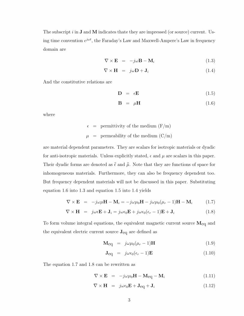
The subscript i in J andM indicates thate they are impressed (or source) current. Us-
ing time convention ejωt, the Faraday’s Law and Maxwell-Ampere’s Law in frequency
domain are
∇× E = −jωB−Mi (1.3)
∇×H = jωD+ Ji (1.4)
And the constitutive relations are
D = ǫE (1.5)
B = µH (1.6)
where
ǫ = permittivity of the medium (F/m)
µ = permeability of the medium (C/m)
are material dependent parameters. They are scalars for isotropic materials or dyadic
for anti-isotropic materials. Unless explicitly stated, ǫ and µ are scalars in this paper.
Their dyadic forms are denoted as ¯ǫ and ¯µ. Note that they are functions of space for
inhomogeneous materials. Furthermore, they can also be frequency dependent too.
But frequency dependent materials will not be discussed in this paper. Substituting
equation 1.6 into 1.3 and equation 1.5 into 1.4 yields
∇× E = −jωµH−Mi = −jωµ0H− jωµ0(µr − 1)H−Mi (1.7)
∇×H = jωǫE+ Ji = jωǫ0E+ jωǫ0(ǫr − 1)E+ Ji (1.8)
To form volume integral equations, the equivalent magnetic current source Meq and
the equivalent electric current source Jeq are defined as
Meq = jωµ0(µr − 1)H (1.9)
Jeq = jωǫ0(ǫr − 1)E (1.10)
The equation 1.7 and 1.8 can be rewritten as
∇× E = −jωµ0H−Meq −Mi (1.11)
∇×H = jωǫ0E+ Jeq + Ji (1.12)
3

Figure 1.1: The demonstration of forward and inverse scattering problems
Furthermore, the total electric filed E and magnetic field H can be divided into
incident fields Ei, Hi and scattered fields Es, Hs. They fit in the equations
∇× Ei = −jωµ0Hi −Mi (1.13)
∇×Hi = jωǫ0Ei + Ji (1.14)
∇× Es = −jωµ0Hs −Meq (1.15)
∇×Hs = jωǫ0Es + Jeq (1.16)
1.3 Motivation of the research
One typical wave propagation is involved with radiated electromagnetic field from a
object due to the illuminating electromagnetic field on the object. The illuminating
field is usually referred as the incident field, which represents the field produced by
the source without the object. The radiated field from the object is referred as the
scattered field. And the object is referred as the scatterer [2]. There are two kinds
of problems in typical wave propagation in the presence of scatters. One is called
forward scattering problem; and the other one is called inverse scattering problem.
As demonstrated in figure 1.1, in a forward scattering problem, the scattered field,
which is the unknown, is evaluated by knowing the incident field and the properties
of the scatterer. In inverse scattering problem, the scattered field (usually partially)
4
and the incident field are usually known, while the properties of the object needs to
be determined.
The Volume and Surface Integral Equations (VSIE) has been used to solving
forward scattering problems in various application successfully. Combined with the
Multi-Level Fast Multipole Method and growing parallel computing techniques, the
volume and surface integral method can be used for computing the scattering prob-
lems of electronically large objects. Several hundred million unknowns’ scattering
problem has been reported solved by using MoM with MLFMM in recent years.
Inverse scattering problems can be found intensively in radar or microwave imag-
ing applications, such as underground imaging, through-wall imaging, biomedical
imaging and so on. It is more difficult to get accurate inverse results than forward
scattering results due to the non-unique solution for the inverse scattering problems.
But for the most of the inverse scattering problems, only part of the scatterer is our
real interest. For example, for through-wall imaging problems, we are only interested
in the objects (such as human beings) beyond the wall. All the other things are
treated as background. Sometimes, we may already has all the information for the
backgrounds. For example, we may already know the property, such as size, location,
permittivity and so on, of the wall and other other background objects. We can use
these pre-known information to increase the accuracy of the objects in interest, such
as the human beings on the other side of the wall, a tumor in the brain.
Here we propose a background subtraction method to increase the quality of
recovered imaging. Since we already know the geometry and the electric property of
the background, its scattered field can be calculated by using VSIE method. With
total scattered field subtracted by the background scattered field, the visibility of
the object in interest can be improved. Before doing the subtraction, some of the
objects may not be able to be recovered due to the interaction between the object
and the background. Some of the weaker scatterers may look like a strong scatterer
or vis versa. After performing the background subtraction, those false information
recovered can be corrected.
5

Chapter 2
Volume and Surface Integral Equations for Complex Objects
Integral equations for solving electromagnetic problem are obtained by applying
boundary conditions to integral representation of the fields [22]. For scattering prob-
lems, we need to get the integral representation of the scattered field (electric field
and/or magnetic field). The scattered field due to harmonically oscillating currents in
free space in the absence of any diffracting body can be represented by integral equa-
tion using dyadic Green’s function [32]. The scattered electric field can be represented
by the dyadic Green’s function as
Es(r) = −jωµ0
∫
¯G0(r, r′) · J(r′)dr′ −
∫
∇G0(r, r′)×M(r′)dr′, (2.1)
where J, M are electric and magnetic current densities respectively. And
¯G0(r, r′) = ( ¯I +
1
k20
∇∇)G0(r, r′) = ( ¯I − 1
k20
∇∇′)G0(r, r′) (2.2)
is called the free-space dyadic Green’s function [32] (electric type), while
G0(r, r′) =
e−jk0|r−r′|
4π|r− r′| (2.3)
is called the scalar Green’s function in free space. The dyadic Green’s function in
equation 2.2 is also called electric dyadic Green’s function, because it transfer the
electric current into electric field. It is the point source response to the vector wave
equation
∇×∇× E(r)− k20E(r) = −jωµ0J(r) (2.4)
in homogeneous medium, where k20 = ω2µ0ǫ0. The
¯I = xx+ yy + zz (2.5)
is called unit dyadic. Unless explicitly specified, the r is always referred to as the
observation point, while r′ is referred as the source point. The magnetic field due to
6

the current densities J and M can be represented by
Hs(r) = −jωε0
∫
¯G0(r, r′) ·M(r′)dr′ +
∫
∇G0(r, r′)× J(r′)dr′. (2.6)
It is also very common to define the magnetic type of dyadic Greens function as [4]
¯Gm0 (r, r
′) = ∇G0(r, r′)× ¯I. (2.7)
Then the scattered electric and magnetic field can be rewritten as
Es(r) = −jωµ0
∫
¯G0(r, r′) · J(r′)dr′ −
∫
¯Gm0 (r, r
′) ·M(r′)dr′, (2.8)
Hs(r) = −jωε0
∫
¯G0(r, r′) ·M(r′)dr′ +
∫
¯Gm0 (r, r
′) · J(r′)dr′. (2.9)
The L and K operators are commonly defined in the literature as
L [J(r′)] = −jk0
∫
¯G0(r, r′) · J(r′) (2.10)
and
K [J(r′)] =
∫
∇G0(r, r′)× J(r′) (2.11)
So the scattered E and H field can be rewritten by using L and K operators as
Es(r) = η0L [J(r′)]−K [M(r′)] (2.12)
Hs(r) =1
η0L [M(r′)] +K [J(r′)] (2.13)
where η0 =√
ε0/µ0 is the wave impedance in free space.
In the following sections, we assume that the magnetic current density M is zero.
We will explore the integral equations for PEC and dielectric objects separately first,
then followed by the integral equations for complex objects. As we explore those
integral equations, you will find that the evaluation of the dyadic Green’s function
are avoid due to its attribute of hyper-singularity. Mathematical remedies used to
avoid that include vector identity, integration by part, the Gauss’s divergence theorem
and so on.
7

Figure 2.1: Scattering by the surface current on PEC
2.1 Surface Integral Equations for Perfect Electric Conductors
Scattering problems of PEC objects can be considered as radiation problems of the
surface currents on the PEC, which are generated by other currents or fields as shown
in figure 2.1. One of the boundary conditions for PEC objects is that on the PEC
surface the tangential component of total electric field on PEC is zero, that is
t · E = t · (Ei + Es) = 0. (2.14)
Or the tangential component of incident field is canceled by the tangential part of
the scattered field, which was due to the induced surface electric current on the PEC,
that is
−t · Ei = t · Es. (2.15)
As assumed M = 0, the electric field integral equation on the PEC can be mathe-
matically represented by
−t · Ei(r) = −jωµ0t ·∫
S′
¯G0(r, r′) · JS(r
′)dr′
= −jωµ0t ·[∫
S′
G0(r, r′)JS(r
′)dr′ − 1
k20
∇∫
S′
∇′G0(r, r′) · JS(r
′)dr′]
= −jωµ0t ·∫
S′
G0(r, r′)JS(r
′)dr′ +j
ωε0t · ∇
∫
S′
∇′G0(r, r′) · JS(r
′)dr′.
(2.16)
where r is on the surface of the PEC object.
8

The EFIE shown in equation 2.16 can be applied on both open and close sur-
faces. And the tangential electric field is continuous across a open PEC surface [8].
For scattering problems of the closed surface objects, the EFIE breaks down on the
internal resonance mode.
The Magnetic Field Integral Equation on the PEC surface is derived from the
extinction theorem, which says that the total tangential magnetic field equals the
induced surface current on PEC.
n×[
Hi(r) +Hs(r)]
= Js(r) (2.17)
where n is the normal direction of the surface. By subtituting the scattered magnetic
field due to the surface current
Hs(r) = ∇×∫
S′
G0(r, r′)Js(r
′)dr′ (2.18)
into equation 2.17, it gives
n×Hi(r) + limr→S+
[
n×∇×∫
S′
G0(r, r′)Js(r
′)dr′]
= Js(r) (2.19)
By doing mathmatical simplification, it can finaly be simplified as [12]
−n×Hi(r) = −1
2Js(r) + n×
∫
S′−δS′
∇G0(r, r′)× Js(r
′)dr′ (2.20)
where δS is a very small, circular region in S located close to r. MFIE can only be
applied on closed surfaces because that the extinction theorem is only valid for closed
surfaces. One of the difference between EFIE and MFIE is that the current on the
PEC surface caused the discontinous of H field, while maitains the continuous of the
E Field across the surface [8].
At the resonance mode, both the EFIE and MFIE will breakdown, a common way
to solve this problem in the literature is to form a combined field integral equation
[5], which use the linear superposition of EFIE and MFIE.
CFIE = αEFIE + η0(1− α)MFIE (2.21)
It is suggested that α is chosen to be about 0.5 by Chew in [8].
9

2.2 Volume Integral Equation for Penetrable Objects Only
The volume integral equation (VIE) are commonly used in solving the scattering
problems for penetrable objects, which can be inhomogeneous and/or anisotropic.
Although, for homogeneous penetrable objects, surface integral equation can be em-
ployed with few unknowns, the VIE still has advantages with simple description of the
scattering with free space Green’s function. Let’s derive the VIEs with the volume
equivalence theorem. According the volume equivalence theorem [2], the volume
equivalent electric and magnetic current densities are defined as
Jeq(r) = jωε0 [εr(r)− 1]E(r) = jωε0τε(r)E(r), (2.22)
Meq(r) = jωµ0 [µr(r)− 1)]H(r) = jωµ0τµ(r)H(r). (2.23)
where τε(r) = [εr(r)− 1] and τµ(r) = [µr(r)− 1)] are denoted as electric and magnetic
contrast coefficient of the penetrable object respectively. The general idea for the
volume integral equation is the total field equals to the summation of the incident
field and the scattered field. The electric and magnetic VIEs are
E(r) = Ei(r) + Es(r) (2.24)
and
H(r) = Hi(r) +Hs(r). (2.25)
And as we did in EFIE or MFIE on PEC, they are also common written in the form
of
−Ei(r) = Es(r)− E(r) (2.26)
and
−Hi(r) = Hs(r)−H(r). (2.27)
There are two different ways to derive electric field VIE. The first one, by substituting
the equation 2.22 and equation 2.8 into the equation 2.26, it gives
− Ei(r)
= −jωµ0
∫
V ′
G0(r, r′)Jeq(r
′)dr′ − j
ωε0∇∫
V ′
∇G0(r, r′) · Jeq(r′)dr′ − E(r)
= k20
∫
V ′
G0(r, r′)τε(r
′)E(r′)dr′ +∇∫
V ′
∇G0(r, r′) · τε(r′)E(r′)dr′ − E(r)
(2.28)
10

By substituting E = D/(ε0εr) into the equation 2.28, the integral equation above can
also be written with D as unknowns as
−ε0Ei(r) = k2
0
∫
V ′
G0(r, r′)χ(r′)D(r′)dr′
+∇∫
V ′
∇G0(r, r′) · χ(r′)D(r′)dr′ − D(r)
εr(r),
(2.29)
where χ = (1− 1/εr). Another format of EFIE can also be derived. By substituting
the equation 2.6 into equation 2.27 gives
−Hi(r) =
∫
V ′
∇G0(r, r′)× J(r′)dr′ −H(r) (2.30)
Applying the curl operation on both sides of the equation 2.30, it gives
−∇×Hi(r) = ∇×∫
V ′
∇G0(r, r′)× J(r′)dr′ −∇×H(r). (2.31)
By substituting ∇ × Hi = jωε0Ei , ∇ × H = jωε0εrE and Jeq = jωε0τεE, the
equation 2.31 can be rewritten as [19]
−Ei(r) = ∇×∫
V ′
∇G0(r, r′)× τε(r
′)E(r′)dr′ − εr(r)E(r). (2.32)
The equations 2.28, 2.29 and 2.32 all can be used to volume integral equations for
penetrable objects. Due to the difference of the boundary condition for different
unknowns and properties for different type basis function, volume integral equation
has to be chosen carefully. In the next chapter we will discuss more of those equation
combined with basis functions.
2.3 Integral Equations for Complex Objects
Here the complex objects are the objects that have both PEC part and penetrable
(dielectric) part. For complex objects, the scattered field can be categorized into two
different types. One is scattered from the surface current of PEC, and the other is
scattered from the equivalent current in the penetrable part. It can be written as
Es = EsV + Es
S, (2.33)
11

where EsS(r) is the scattered electric field due to the PEC surface current, and Es
V (r)
is the scattered electric field due to the equivalent current in penetrable part of
the object. The subscript V and S in equation 2.33 is used to indicate that the
scattered field is contributed by volume and surface sources, respectively. The integral
equations for complex objects can be obtained by using the scattered field form both
types of sources. The format of the scattered field equation may also need to be
adjusted for different types of basis functions and for the convenience of the numerical
evaluation.
On the surface of the PEC part of the objects, the tangential component of total
electric field is zero. In other words, the tangential component of the total scattered
electric field cancels out the tangential component of incident electric field, as
−t · Ei(r) = t · (EsS + Es
V ) . (2.34)
Substituting the scattered field on the PEC surface
EsS(r) = −jωµ0
∫
S′
G0(r, r′)JS(r
′)dr′ +j
ωε0∇∫
S′
∇′G0(r, r′) · JS(r
′)dr′, (2.35)
the scattered field in the dielectric volume
EsV (r) = −jωµ0
∫
V ′
G0(r, r′)Jeq(r
′)dr′ − j
ωε0∇∫
V ′
∇G0(r, r′) · Jeq(r′)dr′, (2.36)
and the equivalent electric current Jeq(r′) = jωε0τε(r
′)E(r′) into the 2.34 gives
−t · EiS(r) = −jωµ0t ·
∫
S′
G0(r, r′)JS(r
′)dr′
+j
ωε0t · ∇
∫
S′
∇′G0(r, r′) · JS(r
′)dr′
+ k20 t ·∫
V ′
G0(r, r′)τε(r
′)E(r′)dr′
+ t · ∇∫
V ′
∇G0(r, r′) · τε(r′)E(r′)dr′.
(2.37)
The SIE in equation 2.37 has the unknowns JS, the surface current on PEC, and the
unknown E, the total electric field inside the penetrate part. Also if we reformat the
equation 2.32, the scattered electric field from volume part can be represented by
EsV (r) = ∇×
∫
V ′
∇G0(r, r′)× τε(r
′)E(r′)dr′ − τε(r)E(r). (2.38)
12

which will lead the EFIE on the PEC to the following format
−t · EiS(r) = −jωµ0t ·
∫
S′
G0(r, r′)JS(r
′)dr′
+j
ωε0t · ∇
∫
S′
∇′G0(r, r′) · JS(r
′)dr′
+∇×∫
V ′
∇G0(r, r′)× τε(r
′)E(r′)dr′ − τε(r)E(r).
(2.39)
It is also easy to change the unknown E to unknown D for a new SIE on PEC as
−t · EiS(r) = −jωµ0t ·
∫
S′
G0(r, r′)JS(r
′)dr′
+j
ωε0t · ∇
∫
S′
∇′G0(r, r′) · JS(r
′)dr′
+k20
ε0t ·∫
V ′
G0(r, r′)χ(r′)D(r′)dr′
+1
ε0t · ∇
∫
V ′
∇G0(r, r′) · χ(r′)D(r′)dr′.
(2.40)
Similarly, the EFIE in the penetrable parts of the complex object can be repre-
sented by
−Ei = Es − E = EsV + Es
S − E (2.41)
There are two obvious ways to get the EsS, the first one is like the way to derive
integral equation 2.32.
EsS(r) = − j
ωε0∇×
∫
S′
∇G0(r, r′)× JS(r
′)dr′ (2.42)
In this case the integral equation in the volume can be written as
−Ei(r) = ∇×∫
V ′
∇G0(r, r′)× τε(r
′)E(r′)dr′ − εr(r)E(r) + EsS
= ∇×∫
V ′
∇G0(r, r′)× τε(r
′)E(r′)dr′ − εr(r)E(r)
− j
ωε0∇×
∫
S′
∇G0(r, r′)× JS(r
′)dr′
(2.43)
The second one to get the scattered field from the surface current is shown in equation
2.35. In that case the integral equation for the penetrable part can be written as
−Ei(r) = ∇×∫
V ′
∇G0(r, r′)× τε(r
′)E(r′)dr′ − εr(r)E(r) + EsS
= ∇×∫
V ′
∇G0(r, r′)× τε(r
′)E(r′)dr′ − εr(r)E(r)
− jωµ0
∫
S′
G0(r, r′)JS(r
′)dr′ +j
ωε0∇∫
S′
∇′G0(r, r′) · JS(r
′)dr′.
(2.44)
13
In the flowing chapters, the EFIE of the complex objects uses the one above. The
integral equation can also written in the form with unknown D and JS based on
equation 2.29 as
−Ei(r) =k20
ε0
∫
V ′
G0(r, r′)χ(r′)D(r′)dr′
+1
ε0∇∫
V ′
∇G0(r, r′) · χ(r′)D(r′)dr′ − D(r)
εr(r)
− jωµ0
∫
S′
G0(r, r′)JS(r
′)dr′ − j
ωε0∇∫
S′
∇′G0(r, r′) · JS(r
′)dr′.
(2.45)
2.4 On selecting unknowns of the EFIE
There are different choices when it comes to choosing unknowns. As shown in the
previous sections, the current J, the electric field intensity E, magnetice field intensity
H and electric flux density D can all be unknowns. It is common to choose J on
surfance and D in volume when the divergence conforming basis function is chosen.
And E is chosen when the curl conforming basis function is used. The reason why it
chosen that way is based on the curl, gradiant and divergence operator in the integral
equations. As we move on to the next chapter, you will find that by choosing certain
unknowns in the chosen EFIE or MFIE, numerical evaluation of these equations can
be simplified as well as some boundary condtions can be automatically met.
14
Chapter 3
The Numerical Solution for the VSIEs
To solve the VSIEs with numerical methods, the integral equations need to be dis-
cretized and converted into matrix equations. In this chapter, the method of moments
will be briefly introduced first. Follow that, two types of basis function will be ex-
plained and applied into the VSIE. In the matrix equations, each element is usually
an integral over a finite domain. Those integration is typically performed by using
numerical quadrature rules. In the cases that the observation point is in the domain
of the integration, the integrand becomes singular and it needs special treatment
when the numerical integration is performed. To solve this problem, the integrand is
either integrated analytically or performed with special numerical treatment, such as
Duffy transformation.
3.1 The Method of Moments
The VSIE is solved numerically by the method of moments. In this method, the
integral equations are discretized into a set of a finite number of linear equations in
a finite number of unknowns [22]. Generally, it solves the linear equation as [14]
Lf = g, (3.1)
where L is a linear operator, g is the excitation or sources, and f is the field or
response. Here, g is a known function and f is the unknown function which is to be
determined. First, the unknown function in the integral equations is expanded by
the basis functions
f =∑
n
αnfn, (3.2)
where αn are constants coefficients, and fn are basis functions. For exact solutions,
3.2 is usually an infinite summation and the fn form a complete set of basis functions.
15
For approximate solutions, the summation is usually truncated with finite number.
Substituting 3.2 into 3.1, and using the linearity of the operator L yields
∑
n
αnLfn = g. (3.3)
An inner product < a, b > is defined as
< a, b >=
∫
a · b dr. (3.4)
Then define a set of testing function wm, and take the inner product on both side of
3.3 with each wm. It gives
∑
n
αn < wm, Lfn >=< wm, g > . (3.5)
The set of equations can be written in matrix format as
Zα = b, (3.6)
where
Z =
< w1, Lf1 > < w1, Lf2 > · · ·< w2, Lf1 > < w2, Lf2 > · · ·
......
. . .
, (3.7)
α =
α1
α2
...
, (3.8)
and
b =
< w1, g >
< w2, g >...
. (3.9)
If the matrix Z is nonsingular, its inverse Z−1 exists. The coefficient can be solved
by
α = Z−1b, (3.10)
and the solution is given by 3.2.
16
There are several issues in using MoM to solve electromagnetic problems. First,
chose a integral equation to appropriately model the EM problem. Second, chose the
basis function to approximate the unknowns. Third, choose the testing function to
test the integrations and transfer the integral equation into a matrix format. Fourth,
solve the matrix format equation. We have discussed the integral equation in the
previous chapter. We will show the basis functions we have used for solving the
VSIEs.
3.2 The Basis Functions
Basis functions are vital in the computational electromagnetics. Choosing basis func-
tions for the certain integral equations is not arbitrary. There are several rules we
have to follow when choosing the right basis functions for a special unknown. The
are several way to classify the basis functions.
First, basis functions can be classified into two groups, scalar basis functions
and vector basis functions. Scalar basis functions are used to expand the scalar un-
knowns, such as a voltage. While vector basis functions are used to expand vector
unknowns, such as electric current, electric field, magnetic field and so on. The vector
basis functions are commonly used in computational electromagnetics. The vector
basis functions used in computational electromagnetics can be further divided into
divergence-conforming basis functions and curl-conforming basis functions. A con-
forming basis maintains certain kind of continuity of the represented unknown on a
sub-sectional model of a surface. The divergence conforming basis function maintains
the first-order continuity needed by the divergence operator, while the curl conform-
ing basis function maintains the first-order continuity needed by the curl operator.
Consequently, a divergence conforming basis function maintains the continuity of the
normal component, while a curl conforming basis function maintains the continuity
of the tangential component [24]. If the unknown is electric flux density D in volume,
it will be appropriate to choose divergence-conforming basis functions. Because it
will automatically enforce the normal continuity for the electric flux density across a
interface. If the unknown is the electric field E in a volume, then it is more appropri-
17
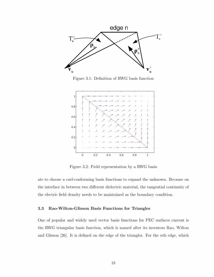
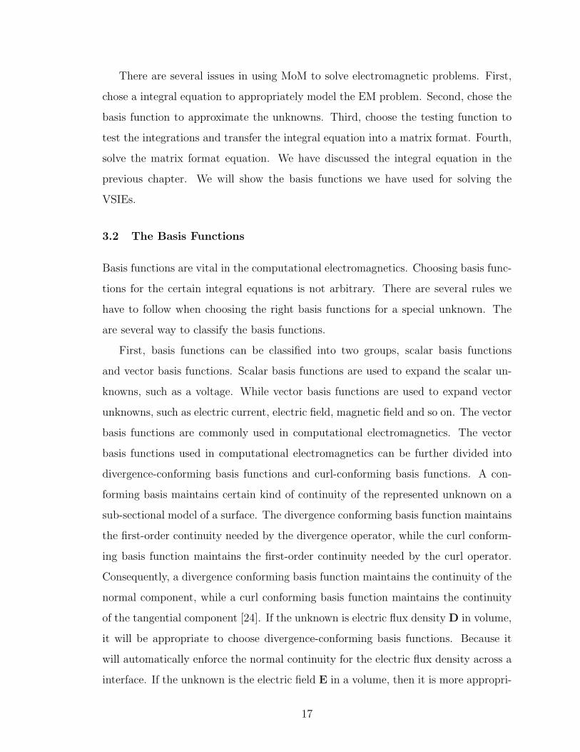
Figure 3.1: Definition of RWG basis function
0 0.2 0.4 0.6 0.8 1
0
0.2
0.4
0.6
0.8
1
Figure 3.2: Field representation by a RWG basis
ate to choose a curl-conforming basis functions to expand the unknown. Because on
the interface in between two different dielectric material, the tangential continuity of
the electric field density needs to be maintained as the boundary condition.
3.3 Rao-Wilton-Glisson Basis Functions for Triangles
One of popular and widely used vector basis functions for PEC surfaces current is
the RWG triangular basis function, which is named after its inventors Rao, Wilton
and Glisson [26]. It is defined on the edge of the triangles. For the nth edge, which
18
is shared by a pair of triangles, as
fSn (r) =
ln2A+
nρ+n (r), r in T+
n
ln2A−
nρ−n (r), r in T−
n
0, otherwise
(3.11)
, where ln is the length of the edge and A±n are the area of the triangle pair T±
n , which
shares the nth edge. And the vector ρ±n (r) are defined as in figure 3.1,
ρ+n (r) = r− v+
n (3.12)
and
ρ−n (r) = v−
n − r. (3.13)
The superscript S in the fSn denotes that it is a surface basis function, which is used
to distinguish from the basis used in volume elements. The RWG basis functions are
associated with interior edges only, which means boundary edges are not associated
with basis functions [12]. The basis function is illustrated in Figure 3.1.
The surface divergence of fSn is
∇S · fSn (r) =
lnA+
n, r in T+
n
−lnA−
n, r in T−
n
0, otherwise
(3.14)
Since there is no accumulate charge on an edge, the RWG basis function is a type
of divergence conforming basis [12]. A field representation by a edge basis is demon-
strated as in figure 3.2. The success of the RWG basis functions is not only because
of the flexibility of modeling arbitrary shape of PEC surface but also its uniquely
role in expanding the surface current by its properties. Following are the properties
which is very important for expanding the surface current [26].
• There are no normal component of current on the exterior boundary, and hence
there is no line charge along exterior boundary.
19
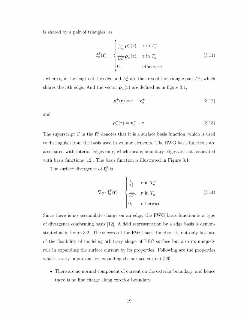
Figure 3.3: A tetrahedron mesh element
• The normal component of the current on an interior edges is constant and
continuous across the edge.
• The total charge associate with the triangle pair is zero.
3.4 Edge Basis Functions for Tetrahedrons
The tetrahedron is a commonly used mesh element for geometrically complex objects
with volume. A tetrahedron is a polyhedron which has four vertices, six edges, and
four triangular faces. After doing the domain discretization by a set of tetrahedrons,
basis functions are usually associated onto those vertices, edges, or faces. The edge
basis function is one of those basis functions associating the basis on each edge of a
tetrahedron. And one edge may be shared by multiple tetrahedrons. Unless specified,
every edge will be associated for one basis function. Later, we will talk about that
those edges who contact with PEC surface can avoid to be associated basis functions.
The nodes and faces are defined on a tetrahedron as shown in 3.3. Then for each
point r inside the tetrahedron, it can be interpolated by local coordinate system as
[15]
r = r0 + L1(r1 − r0) + L2(r2 − r0) + L3(r3 − r0)
= L0r0 + L1r1 + L2r2 + L3r3
(3.15)
where ri (i = 0, 1, 2, 3) are the vertices of the tetrahedron and the Li (i = 0, 1, 2, 3) can
be considered as the local coordinates or simplex coordinates. Every three simplex
coordinates out of the four are linearly independent. Four coordinates are linearly
20

dependent and can be represented by
L0 + L1 + L2 + L3 = 1. (3.16)
Define the unitary vectors ai, the Jacobian√g and reciprocal unitary vectors ai of
edge i node i0 node i10 1 21 0 12 0 23 0 34 2 35 3 1
Table 3.1: Edge definition of a tetrahedron
face i node i0 node i1 node i20 1 2 31 0 3 22 0 1 33 0 2 1
Table 3.2: Face definition of a tetrahedron
a tetrahedron as [31]
ai =∂r
∂Li
= ri − r0 where i = 1, 2, 3 (3.17)
√g = a1 · (a2 × a3) (3.18)
ai = ∇Li (3.19)
For tetrahedrons, they can be written as,
a1 =1√ga2 × a3, a2 =
1√ga3 × a1, a3 =
1√ga1 × a2, a0 = −a1 − a2 − a3 (3.20)
Then the edge basis function in tetrahedron elements is defined as [15]
fVi = li(Li0ai1 − Li1a
i0) (3.21)
21
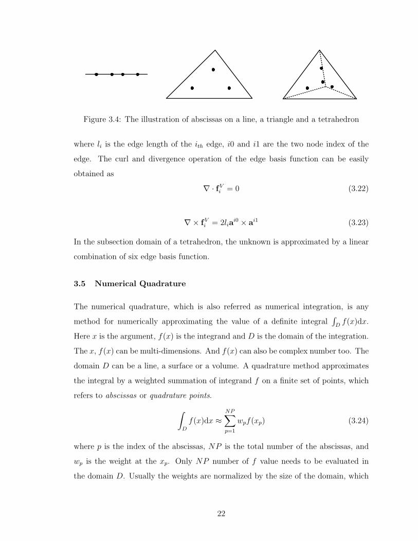
Figure 3.4: The illustration of abscissas on a line, a triangle and a tetrahedron
where li is the edge length of the ith edge, i0 and i1 are the two node index of the
edge. The curl and divergence operation of the edge basis function can be easily
obtained as
∇ · fVi = 0 (3.22)
∇× fVi = 2liai0 × ai1 (3.23)
In the subsection domain of a tetrahedron, the unknown is approximated by a linear
combination of six edge basis function.
3.5 Numerical Quadrature
The numerical quadrature, which is also referred as numerical integration, is any
method for numerically approximating the value of a definite integral∫
Df(x)dx.
Here x is the argument, f(x) is the integrand and D is the domain of the integration.
The x, f(x) can be multi-dimensions. And f(x) can also be complex number too. The
domain D can be a line, a surface or a volume. A quadrature method approximates
the integral by a weighted summation of integrand f on a finite set of points, which
refers to abscissas or quadrature points.
∫
D
f(x)dx ≈NP∑
p=1
wpf(xp) (3.24)
where p is the index of the abscissas, NP is the total number of the abscissas, and
wp is the weight at the xp. Only NP number of f value needs to be evaluated in
the domain D. Usually the weights are normalized by the size of the domain, which
22

make the line, surface and volume quadrature approximation looks like
∫
L
f(r)dr ≈ LNP∑
p=1
Wpf(rp), (3.25)
∫
S
f(r)dr ≈ A
NP∑
p=1
Wpf(rp), (3.26)
and∫
V
f(r)dr ≈ V
NP∑
p=1
Wpf(rp), (3.27)
where L, A, and V are the length of line, the area of the surface and the volume of
the domain respectively. The Wp is the normalized weight at the quadrature point rp.
Notice that the x is replaced by the rp for the argument in 3D space. The abscissas
on a line, on a triangle and in a tetrahedron may looks like figure 3.4.
Different quadrature methods may evaluate different sets of abscissas and their
corresponding weights. We will not discuss how to design a quadrature method. We
pick one of the existed quadrature method for our application which can give desired
accuracy with less number of abscissas. In general, the abscissas are given by the
local coordinate, such as L0, L1, L2 for triangle elements.
The major factors to affect the difficulty of the numerical quadrature is the
smoothness of the integrand as well as the dimension the integral argument. The
smoother the integrand, the easier to perform the numerical quadrature with lesser
quadrature points. For example, if the integrand is a constant all over the integration
domain D, only one point needs to be evaluated. Usually the singularity of the inte-
grand is a hinder to perform a numerical quadrature. The higher order the singularity
is the integrand, the more difficult to get a desired approximation (such as much more
points may needed or even fail). Furthermore, most of the quadrature method are
designed for non-singular integrand. That’s why we need to do mathematical trick
to avoid singular integration (integral with singular integrand or analytical result).
23
Figure 3.5: The local coordinate system for a line element
3.6 The Local Coordinate for a Line Element
A linear line element are usually defined by two points and the edge between the two
points. A local coordinate system is shown as 3.5. A point on the line element is
represented by the local coordinate L1. The global coordinate of the point r can be
obtained by
r = r0 + L1(r1 − r0) (3.28)
where r = (x, y, z), r0 = (x0, y0, z0), and r1 = (x1, y1, z1) in global coordinate system.
It also common to define another auxiliary coordinate L0 = 1− L1, which makes
r = L0r0 + L1r1. (3.29)
Where the L0 is a dependent variable. It is done so to avoid to figure out on a line,
which node is r0 and which one is r1. And if there are multipe line elements, which
usually is the case, each nodes are treated in the same way.
3.7 The Local Coordinate for Triangular Element
A linear triangular element is shown in figure 3.6, which is formed by three vertices
r0, r1, and r2 and three edges between any two of the three vertices. The coordinates
or the vertices are usually defined in global coordinate system, such as Cartesian
coordinate system as (x, y, z). There are a lot of cases such as to perform a numerical
quadrature that a local coordinate system is needed to be defined. This is a must
when a numerical quadrature is performed. As shown in figure 3.6, a point in side the
triangle are uniquely defined by the local coordinate (L1, L2). The origin of the local
coordinate system is set at r0, Knowing the global coordinates of all three vertices,
24
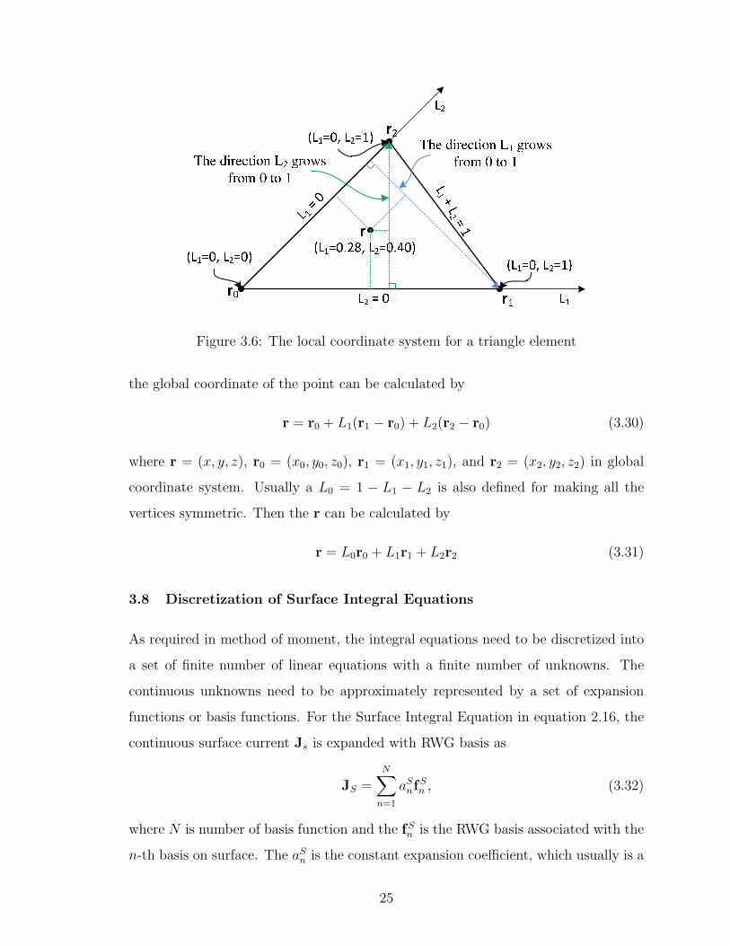
Figure 3.6: The local coordinate system for a triangle element
the global coordinate of the point can be calculated by
r = r0 + L1(r1 − r0) + L2(r2 − r0) (3.30)
where r = (x, y, z), r0 = (x0, y0, z0), r1 = (x1, y1, z1), and r2 = (x2, y2, z2) in global
coordinate system. Usually a L0 = 1 − L1 − L2 is also defined for making all the
vertices symmetric. Then the r can be calculated by
r = L0r0 + L1r1 + L2r2 (3.31)
3.8 Discretization of Surface Integral Equations
As required in method of moment, the integral equations need to be discretized into
a set of finite number of linear equations with a finite number of unknowns. The
continuous unknowns need to be approximately represented by a set of expansion
functions or basis functions. For the Surface Integral Equation in equation 2.16, the
continuous surface current Js is expanded with RWG basis as
JS =N∑
n=1
aSnfSn , (3.32)
where N is number of basis function and the fSn is the RWG basis associated with the
n-th basis on surface. The aSn is the constant expansion coefficient, which usually is a
25

Figure 3.7: Boundary edges of open surface are not basis’ edges
complex value. The PEC surface is meshed with triangles. Only inner edges, which
are shared by two or more mesh triangles, are associated with RWG basis [12]. The
boundary edges on open surface shown as in figure 3.7 (in red color) are not basis
edges. The EFIE 2.16 can be rewritten as
−t · Ei(r) = η0
N∑
n=1
aSnL[fSn ] (3.33)
where
L[fSn ] = −jk0
∫
S′
¯G0(r, r′) · fSn dr′
= −jk0
∫
S′
G0(r, r′)fSn dr
′ + j1
k0∇∫
S′
∇′G0(r, r′) · fSn dr′ (3.34)
Here r is on the PEC surface. Testing the EFIE 3.33 with the testing functions fSm,
which can be the same as the basis function, gives
⟨
fSm,−Ei(r)⟩
= η0
N∑
n=1
aSn⟨
fSm,L[fSn ]⟩
(3.35)
Switch the left hand side with the right hand side, and rewrite the equation with
simplified symbol asN∑
n=1
aSnZSSmn = bSm (3.36)
26

Figure 3.8: The illustration of the normal direction of triangle elements
where ZSSmn = η0
⟨
fSm,L[fSn ]⟩
and bSm =⟨
fSm,−Ei(r)⟩
If the Galerkin’s projection
method is used, which use the basis functions as the testing functions, N equations
(m=1,2,3. . . N) can be formed as in 3.36. Put them together and write it in matrix
format as
ZSS11 ZSS
12 · · · ZSS1N
ZSS21 ZSS
22 · · · ZSS2N
......
. . ....
ZSSN1 ZSS
N2 · · · ZSSNN
as1
as2...
asN
=
bs1
bs2...
bsN
(3.37)
Solving the matrix above will give the coefficients aSn (n=1,2,. . . , N). Then the surface
current JS can be obtained by equation 3.32.
3.9 Evaluation of the Matrix Element
Since the dyadic Green’s function is hyper singular when the R approaches to zero,
it is hard to evaluate the ZSSmn numerically. Therefore, mathematic tricks needs to be
applied to reduce the singularity of the integrands. Expand the impedance elements
as
ZSSmn = η0
⟨
fSm,L[fSn ]⟩
= −jωµ0
∫
S
fSm(r) ·∫
S′
¯G0(r, r′) · fSn (r′)dr′dr
= −jωµ0
∫
S
fSm(r) ·∫
S′
G0(r, r′)fSn (r
′)dr′dr
+j
ωε0
∫
S
fSm(r) · ∇∫
S′
∇′G0(r, r′) · fSn (r′)dr′dr (3.38)
By applying the vector identity
∇′G0(r, r′) · fSn (r′) = ∇′ · [fSn (r′)G0(r, r
′)]−∇′ · fSn (r′)G0(r, r′), (3.39)
27

the gradient operation on the Green’s function can be transfered to the basis function
as
∫
S′
∇′G0(r, r′)·fSn (r′)dr′ =
∫
S′
∇′·[fSn (r′)G0(r, r′)]dr′−
∫
S′
∇′·fSn (r′)G0(r, r′)dr′ (3.40)
By using Gauss’ theorem, the first term on the right hand of the equation 3.40 can
be rewritten as
∫
S′
∇′ · [fSn (r′)G0(r, r′)]dr′ =
∮
ΓS′
n · fSn (r′)G0(r, r′)dl = 0 (3.41)
where the n is the normal direction on the boundary of triangle elements. The term in
3.41 becomes zero because n and fSn are perpendicular to each other on the boundary
shown as in figure 3.8 So,
∫
S′
∇′G0(r, r′) · fSn (r′)dr′ = −
∫
S′
∇′ · fSn (r′)G0(r, r′)dr′ (3.42)
Similarly, the other gradient operation ∇ can be transfered to the testing function
fSm. The impedance matrix element ZSSmn can be rewritten as
ZSSmn = −jωµ0
∫
S
fSm(r) ·∫
S′
G0(r, r′)fSn (r
′)dr′dr
+j
ωε0
∫
S
∇ · fSm(r)∫
S′
∇′ · fSn (r′)G0(r, r′)dr′dr (3.43)
This is done so because that reduce the singulartity from 1/R2 to 1/R for surface
integraton, and the other one is the ∇· fSm(r) and ∇′ · fSn (r′) are well defined and easy
to be evaluated for the RWG basis function in the triangles.
3.10 Calculation of Far Field and RCS
As all the coefficients have been solved, the surface current on the PEC surface can
be calculated through equation 3.32. Therefore, the scattered electric field due to the
surface current can be obtained by Es = η0L[Js]. For far field, it k0R ≫ 1, it can be
simplified as
Es(r) = −jωµ0
∫
S′
G0(r, r′)JS(r
′)dr′ = −jωµ0
N∑
n
aSn
∫
S′
G0(r, r′)fSn (r
′)dr′. (3.44)
28
The approximation can be understood this way. Since the G0(r, r′) ∝ ωµ0
Rand
∇∇G0(r, r′) ∝ 1
ωε0R3 , to make the approximation in equation 3.44 accurate, G0(r, r′) ≫
∇∇G0(r, r′). That is
ωµ0
R≫ 1
ωε0R3⇔ k0R ≫ 1. (3.45)
For far field, the distance between the observation point r and the object is far greater
than the extension of the scatterer,
G0(r, r′) ≈ e−jk0r
4πrejk0r
′·r (3.46)
So the scattered field can be evaluated as
Es(r) =−jωµ0e
−jk0r
4πr
N∑
n
aSnAn
NP∑
p
W Sp e
jk0r′p·rfSn (r′p) (3.47)
where W Sp is the weight of the numerical quadrature, An is the area of the triangle.
The r′p is the source point where the value of the basis function is evaluated. The
fSn (r′p) is evaluates as discussed in matrix element evaluation.
The Radar Cross Section is defined as
RCS = limr→∞
4πr2|Es(r)|2|Ei|2 (3.48)
The RCS are normally symboled as σ. Since the electric field is a vector, polarization
are usually considered for the measurement. There are four combination when both
the incident and scattered field polarization are considered, σθθ, σφθ, σθφ, σφφ. The
first direction in the subscript is direction the measured scattered field, while the
second direction is the direction of the incident field. For example, the σφθ is called
φθ polarization, where the incident field is in the θ direction, and scattered field in
only measured in φ direction. And usually the magnitude of the incident field are
set as one to simplify the RCS calculation. Conventionally, the θ polarization is also
called vertical polarization, while the φ polarization is called horizontal polarization.
In that situation, the polarization is also written as σV V , σV H , σHV , and σHH . The
subscript V represents vertical polarization, while the H represents the horizontal
polarization.
29

0 20 40 60 80 100 120 140 160 180
-8
-6
-4
-2
0
2
4
θ (DEG)
RC
S (
dBsm
)
θθφφMIE-θθMIE-φφ
Figure 3.9: The RCS of PEC sphere with radius as 0.4m
3.11 The Numerical Results for SIE Only
To test the accuracy of the SIE, several test cases has been done using the program
I have developed. The first case is a metal sphere. The radius of the sphere is
R = 0.4m. The frequency is at f = 0.3GHz. The sphere is meshed with 478 triangle
elements with edge size dl = 0.1m. The number of unknown is 717. The mono-static
RCS result is shown in figure 3.9 with θθ and φφ polarizations.
The second case is from EMCC wedge cylinder plate, which geometry is shown in
figure 3.10. The wedge cylinder plate is meshed with 741 triangle element in Cubit
11.1. The The mono-static result with θ = 80 degree comparing with measurements
is shown in figure 3.11, where the measurement is from [20].
30

Figure 3.10: The geometry of the EMCC wedge cylinder plate model
Figure 3.11: The mono-static RCS (in dBλ2) of wedge cylinder plate
31

3.12 Discretization of the Volume and Surface Integral Equations
As required in method of moment, the integral equations need to be discretized into
a set of finite number of linear equations in a finite number of unknowns. The
continuous unknowns need to be approximately represented by a set of expansion
functions or basis functions. For VSIE, there are usually two different unknowns
as we discussed in previous chapter. We will pick the integral equation 2.37 on
PEC surface and integral equation 2.44 in dielectric volume for discretization. Both
equations have two different unknowns JS and E. To discretize the EFIEs, the total
electric field density is expanded by the volume basis functions fV as
E =∑
n∈NV
aVn fVn , (3.49)
where the NV is the set of index number in the volume. And the surface current
density on PEC is expanded by the surface basis functions fS as
JS =∑
n∈NS
aSnfSn , (3.50)
where the NS is the set of index number on the surface. The aSn and aVn are constant
expansion coefficients ( complex numbers ) in equations 3.49 and 3.50, which are to be
determined. The subscriptions V , S in basis functions denote that the basis function
is for volume elements and surface elements respectively. NV is a set of number n
which are in the volume, while NS is the number set of all n on PEC surface. To
convert the EFIEs for complex objects into matrix equations, the extended Galerkin’s
method is used [7]. The extended Galerkin’s method likes the Galerkin’s method,
which uses the testing functions the same as the basis functions. Since there are two
sets of basis functions to expand the integral equations for complex objects, there are
two sets of testing functions too. There are testing functiond for EFIE in volume and
EFIE (and MFIE) on PEC. We will take a example for testing one of the integral
equation in the dielectric volume.
32

Substituting equation 3.49 and 3.32 into equation 2.44, we have
−Ei(r) =∑
n∈NV
aVn∇×∫
V ′
∇G0(r, r′)× τε(r
′)fVn (r′)dr′ − εr(r)∑
n∈NV
aVn fVn (r)
− jωµ0
∑
n∈NS
aSn
[∫
S′
G0(r, r′)fSn (r
′)dr′ − 1
k20
∇∫
S′
∇′G0(r, r′) · fSn (r′)dr′
]
=∑
n∈NV
aVnKV (fVn ) +
∑
n∈NS
aSnLS(fSn )
(3.51)
where the KV and LS are two linear operators operating in volume and on PEC basis
functions separately. And they are defined as
KV (fV ) = ∇×∫
V ′
∇G0(r, r′)× τε(r
′)fV (r′)dr′ − εr(r)fV (r) (3.52)
and
LS(fS) = −jωµ0
[∫
S′
G0(r, r′)fS(r′)dr′ − 1
k20
∇∫
S′
∇′G0(r, r′) · fS(r′)dr′
]
= −jωµ0
∫
S′
G0(r, r′)fS(r′)dr′ +
j
ωε0∇∫
S′
∇′G0(r, r′) · fS(r′)dr′ (3.53)
Converting the equation 3.51 into matrix equation by testing both sides with basis
functions in the volume. For the testing function fVm , it gives
< fVm(r),−Ei(r) >=∑
n∈NV
aVn < fVm(r), KV (fVn ) >+∑
n∈NS
aSn < fVm(r), LS(fSn ) >.
(3.54)
By letting
ZV Vmn = < fVm(r), KV (fVn ) >
=
∫
V
fVm(r) · ∇ ×∫
V ′
∇G0(r, r′)× τε(r
′)fVn (r′)dr′dr
−∫
V
fVm(r) · εr(r)fV (r)dr, (3.55)
ZV Smn = < fVm(r), LS(fSn ) >
= −jωµ0
∫
V
fVm(r) ·∫
S′
G0(r, r′)fS(r′)dr′dr
+j
ωε0
∫
V
fVm(r) · ∇∫
S′
∇′G0(r, r′) · fS(r′)dr′dr. (3.56)
33

and
bVm =< fVm(r),−Ei(r) >= −∫
V
fVm(r) · Ei(r)dr (3.57)
and put bVm on the right hand side, the 3.54 can be rewritten as
∑
n∈NV
aVnZV Vmn +
∑
n∈NS
aSnZV Smn = bVm (3.58)
Similarly, for the integral equation for PEC parts, the equation 2.37 can be ex-
panded as
−t · EiS(r) =
∑
n∈NS
aSn t · LS(fSn ) +NV∑
n
aVn t · LV (fVn ), (3.59)
where
LS(fSn ) = −jωµ0
∫
S′
G0(r, r′)fSn (r
′)dr′ +j
ωε0∇∫
S′
∇′G0(r, r′) · fSn (r′)dr′, (3.60)
and
LV (fVn ) = k20
∫
V ′
G0(r, r′)τε(r
′)fVn (r′)dr′ +∇∫
V ′
∇G0(r, r′) · τε(r′)fVn (r′)dr′ (3.61)
Testing the equation 3.59 with the RWG basis on PEC surface, we get
< fSm,−EiS >=
∑
n∈NS
aSn < fSm, LS(fSn ) >+
∑
n∈NV
aVn < f sm, LV (fVn ) >. (3.62)
The impedance matrix element ZSSmn and ZSV
mn are defined as
ZSSmn = < fSm, L
S(fSn ) >
= −jωµ0
∫
S
fSm(r) ·∫
S′
G0(r, r′)fSn (r
′)dr′dr
+j
ωε0
∫
S
fSm(r) · ∇∫
S′
∇′G0(r, r′) · fSn (r′)dr′dr, (3.63)
ZSVmn = < f sm, L
V (fVn ) >
= k20
∫
S
fSm(r) ·∫
V ′
G0(r, r′)τε(r
′)fVn (r′)dr′dr
+
∫
S
fSm(r) · ∇∫
V ′
∇G0(r, r′) · τε(r′)fVn (r′)dr′dr. (3.64)
In equation 3.62 The t· is gone because that the fSm has only tangential component
on the PEC surface. By letting
bSm =< fSm,−EiS >= −
∫
S
fSm · EiSdr, (3.65)
34

and putting it on the right hand side, the equation 3.62 can be rewritten as
∑
n∈NV
aVnZSVmn +
∑
n∈NS
aSnZSSmn = bSm (3.66)
Put the equations 3.58 and 3.66 together and rewrite them into matrix form
ZV V ZV S
ZSV ZSS
aV
aS
=
bV
bS
(3.67)
where aV and aS are vectors of the expansion coefficients formed by aVn with n ∈ NV
and aVn with n ∈ NS separately. And bV and bS are the excitation vectors for surface
and volume elements formed by bVm with m ∈ NV and bSm with m ∈ NS respectively.
3.13 Numerical Evaluation of the Impedance Matrix Elements VV and
VS
The integrals for the impedance matrix elements are usually evaluated by numerical
quadratures, which use weighted summations to approximate integrations. When the
observation point is in the source element, the Green’s function and its derivatives
are singular. Their singularity has been shown in the appendix. Generally, the more
times derivative operated on the Green’s function, the higher singularity is the result.
Since the numerical quadrature rules tend to fail in the cases of singular integrands for
required accuracy. The singular extraction method or Duffy transformation are usu-
ally used to increase the numerical accuracy. In this section, the numerical evaluation
of ZV Vmn and ZV S
mn will be discussed.
To evaluate the ZV Vmn , we define a auxiliary function ΨV
n as
ΨVn (r) =
∫
V ′
∇G0(r, r′)× τε(r
′)fVn (r′)dr′ (3.68)
the representation of ZV Vmn in equation 3.55 can be rewritten as
ZV Vmn =
∫
V
fVm(r) · ∇ ×ΨVn (r)dr−
∫
V
fVm(r) · εr(r)fVn (r)dr. (3.69)
There is no singularity on the second term on the right hand side of equation 3.69.
It is not zero only when fVm overlaps fVn , or when the two edges which are associated
35

with the two basis functions are in the same element (such as a tetrahedron). It can
be numerically evaluated by
∫
V
fVm(r) · εr(r)fVn (r)dr =∑
i
Vi
NP∑
p=1
WpfVm(rp) · εr(rp)fVn (rp). (3.70)
where
rp = L0[p]r0 + L1[p]r1 + L2[p]r2 + L3[p]r3, (3.71)
is the point at which the integrand will be evaluated and the Wp is the weight at
the point for the numerical quadrature in the tetrahedron. The r0, r1, r2 and r3 are
the four vertices of the test tetrahedron, while the L0, L1 L2 and L3 are the simplex
coordinates of the tetrahedron. The first summation∑
i on the right hand side of
the equation 3.70 is because that a edge can be shared by multiple volume elements
(tetrahedrons). Vi is the volume of the i-th element where the edges m and n reside.
If the permittivity εr in each volume element is homogeneous and isotropic, which is
the case we are testing, analytic solution can be obtained for tetrahedron elements,
since
∫
Vi
fVm(r) · fVn (r)dr =
∫
Vi
lm(
Lm0am1 − Lm1a
m0)
· ln(
Ln0an1 − Ln1a
n0)
dr
= lmln(am1 · an1
∫
Vi
Lm0Ln0dr− am1 · an0
∫
Vi
Lm0Ln1dr
−am0 · an1
∫
Vi
Lm1Ln0dr+ am0 · an0
∫
Vi
Lm1Ln1dr).(3.72)
In equation 3.72, am0, am1, an0 and an1 are constant in the tetrahedron (for linear
tetrahedron only). Lm0, Lm1, Ln0 and Ln1 are functions of space. The following
integration can be analytically get for tetrahedrons.
∫
LmLndr =
160
if n 6= m
1120
if n = m
(3.73)
where m = 0, 1, 2, 3 and n = 0, 1, 2, 3 are the local index of the four edges.
36
The first integral on the right side of equation 3.69 can be evaluated by∫
V
fVm(r) · ∇ ×ΨVn (r)dr
=
∫
V
ΨVn (r) · ∇ × fVm(r)dr−
∫
V
∇ ·[
fVm(r)×ΨVn (r)
]
dr
=
∫
V
ΨVn (r) · ∇ × fVm(r)dr−
∮
ΓV
[
fVm(r)×ΨVn (r)
]
· ndS
(3.74)
where the ΓV is the bounding surface of the volume element for the second surface
integral term on the right hand side. And the n is norm of the surface toward the
outside. The Gauss’ divergence theorem is applied from the volume integration to
the surface integration. By doing this, one of the derivative to the Green’s function
in (∇×ΨVn (r)) has been transfered to the derivative to the basis function (∇× fVm).
The first integral on the right hand side of equation 3.74 can be numerically evaluated
by
∫
V
ΨVn (r) · ∇ × fVm(r)dr = 2lm
∑
i
Vi(am0i × am1
i ) ·NP∑
p=1
WpΨVn (rp). (3.75)
The∑
i is the summation for all the tetrahedrons that both the fVm and fVn reside.
The subscript i for am0i and am1
i denotes that those reciprocal unitary vectors are for
the i-th volume. The second integral term on the right hand side of equation 3.74
can be numerically evaluated by applying quadrature rules on the triangle element,
∮
ΓV
[
fVm(r)×ΨVn (r)
]
· ndS =∑
i
Ai
NP∑
p=1
Wp
[
fVm(rp)×ΨVn (rp)
]
· ni (3.76)
where Ai is the area and ni is the norm of the i-th triangle. The fVm(rp) can be
evaluated by
fVm(rp) = lm(
Lm0[p]am1 − Lm1[p]a
m0)
(3.77)
So far, we have not discussed the evaluation of the Ψn(rp). For the cases that
the observation point rp is not in the source volume and not on the boundary of the
source volume (rp 6= r′ for all the r′ in the volume). Ψn(rp) can be evaluated directly
by numerical quadrature by
ΨVn (rp) =
∑
j
Vj
NQ∑
q=1
Wq∇G0(rp, rq)× τε(rq)fVn (rq), (3.78)
37
where
rq = L0[q]r′0 + L1[q]r
′1 + L2[q]r
′2 + L3[q]r
′3. (3.79)
The gradient of the Green’s function can be evaluated by
∇G0(rp, rq) =
[− cos(k0R)− k0R sin(k0R)
4πR2+ j
sin(k0R)− k0R cos(k0R)
4πR2
]
R, (3.80)
where R = |rp−rq| and R is the normalization for vector R = rp−rq. When the test
function overlaps with the basis function, the R can become zero when the observation
point rp is overlapped with the source point rq. In that case, the integrand of Ψn
becomes singular due to the singularity of the ∇G0. As we show in the appendix ,
the gradient of the Green’s function has the same order of singularity as R/R2. In
that case, the singularity part needs to be extracted and evaluated by other methods.
And the remaining nonsingular part is still evaluated by numerical quadrature.
ΨVn (rp) =
∫
V ′
[
∇G0(rp, r′) +
R
4πR2
]
× τε(r′)fVn (r′)dr′
− 1
4π
∫
V ′
1
R2R× τε(r
′)fVn (r′)dr′
= I1 − I2
(3.81)
The first integral term I1 in the equation 3.81 has no singularity and hence can be
numerically evaluated.
I1 =
∫
V ′
[
∇G0(rp, r′) +
R
4πR2
]
× τε(r′)fVn (r′)dr′
≈∑
j
Vj
NQ∑
q=1
Wq
[
∇G0(rp, rq) +R
4πR2
]
× τε(rq)fVn (rq)
(3.82)
where
∇G0(rp, rq) +R
4πR2=
[
1− cos(k0R)− k0R sin(k0R)
4πR2+ j
sin(k0R)− k0R cos(k0R)
4πR2
]
R
(3.83)
The second integral term I2 is the singular term. And it can be numerically evaluated
by using Duffy transformation. As shown in the appendix
I2 =1
4π
∫
V ′
R
R2× τε(r
′)fVn (r′)dr′ (3.84)
38

To evaluate the ZV Smn , we define
ΦSn(r) =
∫
S′
∇′G0(r, r′) · fSn (r′)dr′ (3.85)
and
ΨSn(r) =
∫
S′
G0(r, r′)fSn (r
′)dr′. (3.86)
By performing integration by parts and applying Gauss’ divergence theorem on the
surface for ΦSn, we have
ΦSn(r) =
∮
ΓS′
[
G0(r, r′)fSn (r
′)]
· ndl −∫
S′
G0(r, r′)∇′ · fSn (r′)dr′
= −∫
S′
G0(r, r′)∇′ · fSn (r′)dr′
The first term on the right hand side of equation 3.87 becomes zero because of the
property of the RWG basis. There is no electric current flowing out of the surface.
And
fVm(r) · ∇ΦSn(r) = ∇ ·
[
ΦSn(r)f
Vm(r)
]
− ΦSn(r)∇ · fVm(r) = ∇ ·
[
ΦSn(r)f
Vm(r)
]
(3.87)
because that ∇· fVm = 0. The impedance matrix element ZV Smn in 3.56 can be rewritten
as
ZV Smn = −jωµ0
∫
V
fVm(r) ·ΨSn(r)dr+
j
ωε0
∫
V
∇ ·[
ΦSn(r)f
Vm(r)
]
dr
= −jωµ0
∫
V
fVm(r) ·ΨSn(r)dr+
j
ωε0
∮
ΓV
ΦSn(r)f
Vm(r) · ndS
(3.88)
It can then numerically evaluated by
ZV Smn = −jωµ0
∑
i
Vi
NP∑
p=1
WpfVm(rp)·ΨS
n(rp)+j
ωε0
∑
i
Si
NS∑
s=1
WsΦSn(rs)f
Vm(rs)·ni (3.89)
where the Wp is the weighting factor in the volume V and the Ws is the weight
factor on the surface. And they are different sets of weighting factors. There is no
singularity for the term ΨSn as long as the testing point is not on the conducting
surface. It is evaluated by
ΨSn(rp) =
∑
i
Si
NQ∑
q=1
WqG0(rp, rq)fSn (rq) (3.90)
39

The ΦSn can be singular when the PEC surface contacts with the outer surface of the
dielectric volume. It can be evaluated in nonsingular cases by
ΦSn(rp) =
lnAn
∑
i
Si
NS∑
s=1
WsG0(rp, r′q) (3.91)
3.14 Numerical Evaluation of the Impedance Matrix Elements SS and
SV
To evaluate the ZSSmn, two auxiliary functions ΦS
n(r) and ΨSn(r) are defined as
ΦSn(r) =
∫
S′
∇′G0(r, r′) · fSn (r)dr′ (3.92)
and
ΨSn(r) =
∫
S′
G0(r, r′)fSn (r)dr
′. (3.93)
By applying the vector identity
∇′G0(r, r′) · fSn (r′) = ∇ ·
[
G0(r, r′)fSn (r
′)]
−G0(r, r′)∇′ · fSn (r′) (3.94)
and Gauss’ theorem, the ΦSn can be rewritten as
ΦSn(r) =
∮
ΓS′
G0(r, r′)fSn (r) · ndl −
∫
S′
G0(r, r′)∇′ · fSn (r′)dr′ (3.95)
The first term of the right hand side in equation 3.95 is zero for RWG basis. This is
because the RWG basis is normally continuous across the edge that the pair triangle
share and it has no tangential component on the other edges as show in figure 3.12.
In that case, the ΦSn can be simplified as
ΦSn(r) = −
∫
S′
G0(r, r′)∇′ · fSn (r′)dr′ (3.96)
Substituting the ΦSn and ΨS
n into the representation of ZSSmn in equation 3.63 yields
ZSSmn = −jωµ0
∫
S
fSm(r) ·ΨSn(r)dr−
j
ωε0
∫
S
fSm(r) · ∇ΦSn(r)dr (3.97)
To evaluate the second term at right hand side in the above equation, we can apply
another vector identity
fSm(r) · ∇ΦSn(r) = ∇ ·
[
ΦSn(r)f
Sm(r)
]
− ΦSn(r)∇ · fSm(r) (3.98)
40

Figure 3.12: The illustration of the normal continuity of a RWG basis function
Substituting the equation 3.98 into equation 3.38 and performing another Gauss’
theorem on the testing triangles, we have
ZSSmn = −jωµ0
∫
S
fSm(r) ·ΨSn(r)dr+
j
ωε0
∫
S
∇ · fSm(r)ΦSn(r)dr (3.99)
The ZSSmn can be numerically evaluated by
ZSSmn = −jωµ0
∑
i
Si
NP∑
p=1
W Sp f
Sm(rp)Ψ
Sn(rp) +
j
ωε0
∑
i
Si
NP∑
p=1
W Sp ∇ · fSm(rp)ΦS
n(rp)
(3.100)
where
rp = L0[p]r0 + L1[p]r1 + L2[p]r2, (3.101)
is the point where the integrand is calculated. The r0, r1 and r2 are the vertices of
the triangle where the edge m resides. In the equation 3.97,
fSm(rp) =lm2Am
ρm(rp) (3.102)
ΨSn(rp) ≈
∑
j
Sj
NP∑
p=1
W Sp G0(rp, rq)f
Sn (rq), (3.103)
ΦSn(rp) ≈ −
∑
j
ln
NP∑
p=1
W Sp G0(rp, rq) (3.104)
To evaluate the ZSVmn , we define two auxiliary functions ΦS
n(r) and ΨSn(r) as
ΦVn (r) =
∫
V ′
∇G0(r, r′) · τε(r′)fVn (r′)dr′ (3.105)
and
ΨVn (r) =
∫
V ′
G0(r, r′)τε(r
′)fVn (r′)dr′. (3.106)
41
After applying vector identity
fSm · ∇ΦVn = ∇ ·
(
fSmΦVn
)
− ΦVn∇ · fSm (3.107)
and Gauss’ theorem, the equation 3.64 can be rewritten as
ZSVmn = k2
0
∫
S
fSm(r) ·ΨVn (r)dr+
∫
ΓS
ΦVn (r)f
Sm(r) · ndl −
∫
S
ΦVn (r)∇ · fSm(r)dr
= ISV1 + ISV2 − ISV3
(3.108)
The ISV1 can be numerically evaluated by
ISV1 = k20
∑
i
Si
NP∑
p=1
W Sp f
sm(rp) · .ΨV
n (rp) (3.109)
The ISV2 is zero for the RGW basis functions. And the ISV3 can be evaluated by
ISV3 = k20
∑
i
Si
NP∑
p=1
W Sp Φ
Vn (rp)∇ · f sm(rp) (3.110)
3.15 Numerical Evaluation of the Right Hand Side
For the evaluation of the right hand side, we usually set the magnitude of the incident
electric field as one, that is
|Ei| = 1. (3.111)
And its directions are usually either θ or φ. So the right hand side bVm are stored with
two component bVmθ and bVmφ.
bVmθ ≈ −θ ·∑
i
Vi
NP∑
p=1
W Vp fVm(rp)e
−jkk·rp (3.112)
bVmφ ≈ −φ ·∑
i
Vi
NP∑
p=1
W Vp fVm(rp)e
−jkk·rp (3.113)
Similarly, the bSmθ and bSmφ are evaluated by
bVmθ ≈ −θ ·∑
i
Si
NP∑
p=1
W Sp f
Sm(rp)e
−jkk·rp (3.114)
bVmφ ≈ −φ ·∑
i
Si
NP∑
p=1
W Sp f
Sm(rp)e
−jkk·rp (3.115)
42
3.16 Singular Integration for the Auxiliary Functions
The integrands of the pre-defined auxiliary functions ΦS, ΦS, ΦV , ΦV and ΨV are
singular when the test point is overlapped with the source point (r = r′). Numerical
integration for singular integrands may rise inaccuracy or error. It is common to
use singular extraction or singularity weakening methods to improve the accuracy.
In the singular extraction method, the integrand is divided into singular part and
non-singular part. The singular part can usually be analytically integrated, while the
non-singular part can be numerical integrated directly. For example,
e−jk0R
R=
(
e−jk0R
R− 1
R
)
+1
R(3.116)
The first term on the right hand side of the equation 3.116 in the parenthesis has no
singularity when R approaches to zero.
ΦSn(r) =
∫
S′
G0(r, r′)fSn (r
′)dr′ =1
4π
∫
S′
e−jkR
RfSn (r
′)dr′
=1
4π
∫
S′
(
e−jkR
R− 1
R
)
fSn (r′)dr′ +
1
4π
∫
S′
1
RfSn (r
′)dr′(3.117)
For triangle elements,
∫
S′
1
Rdr′ =
∫
S′
1
|r− r′|dr′
=3∑
i=1
P 0i · ui
[
P 0i log
R+i + l+i
R+i + l+i
−|d|(
tan−1 P 0i l
+i
(R0i )
2 + |d|R+i
− tan−1 P 0i l
−i
(R0i )
2 + |d|R−i
)]
(3.118)
3.17 Calculation of Far Field and RCS
As all the coefficient have been solved, the scattered field from the PEC surface and
dielectric volume (penetrable part) can be calculate by the expansion function. And
the total scattered field is the summation of the two type of scattered field. The
43

scattered far field from PEC surface can be calculate by
EsS(r) = −jωµ0
∫
S
G0(r, r′)JS(r
′)dr′ = −jωµ0
NS∑
n=1
aSn
∫
S
G0(r, r′)fSn (r
′)dr′
≈ −jωµ0
4π
e−jk0r
r
NS∑
n=1
aSn
∫
S
fSn (r′)ejk0r
′·rdr′
≈ −jωµ0
4π
e−jk0r
r
NS∑
n=1
aSnln2An
∫
S
ρn(r′)ejk0r
′·rdr′
≈ −jωµ0
4π
e−jk0r
r
NS∑
n=1
aSnln2
NP∑
p=1
Wpρn(r′p)e
jk0r′p·rdr′
(3.119)
where r = |r| and r = r/r are the distance and direction of the observation point.
The NS is the number of RWG basis, and the NP in equation 3.119 is the number
of quadrature point on each triangle. In programming practice, doing the summation∑
n=1 NS iterates all the edges except the exterior edges. And shared edges must be
iterated all the triangles it resides. It is also practical and efficient to iterate all the
triangles first and for each triangle iterate all its three edges except those exterior
edges.
Similarly, the scattered far field from the dielectric part (the equivalent current)
can be calculated by
EsS(r) = −jωµ0
∫
V
G0(r, r′)Jeq(r
′)dr′ = k20
NV∑
n=1
aVn
∫
S
G0(r, r′)τε(r
′)fSn (r′)dr′
≈ k20
4π
e−jk0r
r
NV∑
n=1
aVn
∫
V
fVn (r′)τε(r′)ejk0r
′·rdr′
≈ k20
4π
e−jk0r
r
NV∑
n=1
aVn ln
∫
V
(Ln0(r′)αn1 − Ln1(r
′)αn0)τε(r′)ejk0r
′·rdr′
≈ k20
4π
e−jk0r
r
NV∑
n=1
aVn lnVn
NP∑
p
Wp(Ln0[p]αn1 − Ln1[p]α
n0)τε(r′p)e
jk0r′p·rdr′
(3.120)
The NV is the number of edge basis in the volume. When doing the summation∑NV
n=1, all the tetrahedrons share the edge need to be iterated. An alternative way to
do that is to iterate tetrahedron outside and to iterate all its six edges inside to be
more efficient.
44
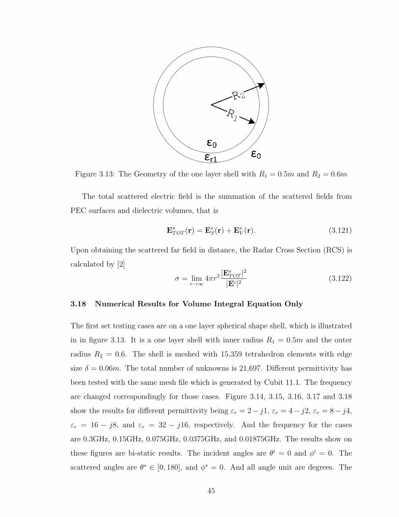
Figure 3.13: The Geometry of the one layer shell with R1 = 0.5m and R2 = 0.6m
The total scattered electric field is the summation of the scattered fields from
PEC surfaces and dielectric volumes, that is
EsTOT (r) = Es
S(r) + EsV (r). (3.121)
Upon obtaining the scattered far field in distance, the Radar Cross Section (RCS) is
calculated by [2]
σ = limr→∞
4πr2|Es
TOT |2|Ei|2 (3.122)
3.18 Numerical Results for Volume Integral Equation Only
The first set testing cases are on a one layer spherical shape shell, which is illustrated
in in figure 3.13. It is a one layer shell with inner radius R1 = 0.5m and the outer
radius R2 = 0.6. The shell is meshed with 15,359 tetrahedron elements with edge
size δ = 0.06m. The total number of unknowns is 21,697. Different permittivity has
been tested with the same mesh file which is generated by Cubit 11.1. The frequency
are changed correspondingly for those cases. Figure 3.14, 3.15, 3.16, 3.17 and 3.18
show the results for different permittivity being εr = 2− j1, εr = 4− j2, εr = 8− j4,
εr = 16 − j8, and εr = 32 − j16, respectively. And the frequency for the cases
are 0.3GHz, 0.15GHz, 0.075GHz, 0.0375GHz, and 0.01875GHz. The results show on
these figures are bi-static results. The incident angles are θi = 0 and φi = 0. The
scattered angles are θs ∈ [0, 180], and φs = 0. And all angle unit are degrees. The
45

0 20 40 60 80 100 120 140 160 180−40
−35
−30
−25
−20
−15
−10
−5
0
5
10
θ
RC
S
θθφφMIE−θθMIE−φφ
Figure 3.14: The RCS of the one layer shell with εr = 2− j1 at 0.3GHz
0 20 40 60 80 100 120 140 160 180
−12
−10
−8
−6
−4
−2
0
2
4
6
θ
RC
S
θθφφMIE−θθMIE−φφ
Figure 3.15: The RCS of the one layer shell result with εr = 4− j2 at 0.15GHz
46

0 20 40 60 80 100 120 140 160 180
-16
-14
-12
-10
-8
-6
-4
-2
0
θ
RC
S
θθφφMIE-θθMIE-φφ
Figure 3.16: The RCS of the one layer shell with εr = 8− j4 at 0.075GHz
0 20 40 60 80 100 120 140 160 180
-35
-30
-25
-20
-15
-10
θ
RC
S
θθφφMIE-θθMIE-φφ
Figure 3.17: The RCS of the one layer shell with with εr = 16− j8 at 0.0375GHz
47

0 20 40 60 80 100 120 140 160 180
-50
-45
-40
-35
-30
-25
-20
θ
RC
S
θθφφMIE-θθMIE-φφ
Figure 3.18: The RCS of the one layer shell with εr = 32− j16 at 0.01875GHz
Figure 3.19: The Geometry of a two layer shell with R1 = 0.5m, R2 = 0.6m andR3 = 0.7m
48

0 20 40 60 80 100 120 140 160 180
-8
-6
-4
-2
0
2
4
6
8
10
θ
RC
S
θθφφMIE-θθMIE-φφ
Figure 3.20: The RCS result of a two layer shell with εr1 = 4.0−j2.0, εr2 = 2.0−j1.0at 0.15GHz
0 20 40 60 80 100 120 140 160 180
-8
-6
-4
-2
0
2
4
θ
RC
S
θθφφMIE-θθMIE-φφ
Figure 3.21: The RCS result of a two layer shell with εr1 = 8.0−j4.0, εr2 = 4.0−j2.0at 0.075GHz
49

0 20 40 60 80 100 120 140 160 180
-25
-20
-15
-10
-5
θ
RC
S
θθφφMIE-θθMIE-φφ
Figure 3.22: The RCS of a two layer shell with εr1 = 16.0− j8.0, εr2 = 8.0− j4.0 at0.0375GHz
0 20 40 60 80 100 120 140 160 180
-45
-40
-35
-30
-25
-20
θ
RC
S
θθφφMIE-θθMIE-φφ
Figure 3.23: The RCS of a two layer shell with εr1 = 32.0− j16.0, εr2 = 16.0− j8.0at 0.01875 GHz
50

Figure 3.24: The Geometry of the coated sphere with R1 = 0.4m, R2 = 0.5m andR3 = 0.6m
unit for the RCS is dBsm. The results are compared with the analytic solution by
MIE series.
We further test the volume integral equation with multi-layer shells. A two layer
spherical shell is shown as in figure 3.19. The inner layer and outer layer are meshed
with tetrahedrons. The size of the tetrahedron of the inner layer is δ1 = 0.06m and the
outer layer is δ2 = 0.1m. The two layer shell share the spherical interface. The inner
shell is composed of 15,359 tetrahedrons, while the outer shell is composed of 12,377
tetrahedrons. The total number of unknowns is 35,010. The bi-static configuration
is the same as the previous case with θi = φi = 0, θs ∈ [0, 180], and φs = 0, all in
degrees. Figure 3.20, 3.21, 3.22, and 3.23 show the results with different εr1, εr2 pair
at different frequencies.
3.19 Numerical Results of Coated Object using VSIE
For hybrid VSIE, we tested a two layer coated PEC sphere as shown in 3.24. The
radius the PEC sphere is 0.4m. And thickness for each layers are 0.1m. The dielectric
constant for its inner coated layer is εr1 = 2.0−j1.5 and outter layer is εr1 = 2.0−j1.5.
With simulation frequency at 0.15GHz, the simulation results of the two layer shell
only and the whole object are compared with MIE results as shown in 3.25 and
3.26. The object is mesh with maximum edge length as 0.07mm. The mesh contains
51

0 20 40 60 80 100 120 140 160 180
−12
−10
−8
−6
−4
−2
0
2
4
6
θ
RC
S
θθφφMIE−θθMIE−φφ
Figure 3.25: The RCS result of two layered shells, where R1 = 0.4m, R2 = 0.5m,R3 = 0.6m, εr1 = 2.0−j1.5, εr2 = 3.0−j1.5, frequency at 0.15 GHz. The comparisonis made to MIE series.
944 triangles on the PEC sphere, 7210 tetrahedrons for the inner layer and 11023
tetrahedrons for the outter layer. The number of total unknowns is 23621.
52

0 20 40 60 80 100 120 140 160 180elevation angle θ
−15
−10
−5
0
5
10
RC
S (
dB
sm)
co2_m4_m5_m6
θθ
φφ
MIE θθ
MIE φφ
Figure 3.26: The RCS result of PEC sphere coated with two layered shells, whereR1 = 0.4m, R2 = 0.5m, R3 = 0.6m, εr1 = 2.0 − j1.5, εr2 = 3.0 − j1.5, frequency at0.15 GHz. The comparison is made to MIE series.
53
Chapter 4
Improve the Efficiency of the VSIE by MLFMM
The VSIE, which is essentially a MoM method, involves of getting a electric response
(E field, H field, and so on) at a point due all the other points. It has a complexity
of O(N2), which is commonly found in N-body problem. Invented by Greengard
and Rokhlin [13], the Fast Multipole Method (FMM) or Fast Multipole Algorithm
(FMA) is used to reduce the complexity of N-body problems. As discussed in previous
chapters, one of the disadvantages of integral equation method is that the impedance
matrix is a full matrix. If an iterative solver is used to solve the problem, matrix-
vector products are performed at each step. A full matrix can be much slower than a
sparse matrix when doing matrix-vector product. In the FMM, sources are grouped.
Electromagnetic field transfered from source point to the observation point which
are not in close groups is divided by three stages. The source point to the source
group. Then the source group to the observation group. And last the observation
group to the observation point. The group to group propagation of the field can be
shared by all the points in the group. The complexity of point to point interaction is
relieved by group to group interaction. The plan wave expansion, radiation function,
receiving function and the transfer function build up the FMM algorithm, which will
be explained in the following sections. By applying the FMM, the matrix-vector
products can be greatly improved, which can improve the efficiency of the VSIE.
4.1 The Gegenbauer’s addition theorem for the Green’s function
The Fast Multipole Methods (FMM) is based on two identities. The first one is the
Gegenbauer’s addition theorem. For time convention e−iwt, it is written as [9]
eik|X+d|
|X+ d| = ik∞∑
l=0
(−1)l(2l + 1)jl(kd)h(1)l (kX)Pl(d · X) (4.1)
54

Figure 4.1: The illustration of geometry X and d for the addition theorem
where jl is a spherical Bessel function of the first kind, h(1)l is the spherical Hankel
function of the first kind and Pl is a Legendre polynomial. The X and d are two
vectors, whose geometry is shown in figure 4.1.
To be consistent, the ejωt time convention will be used. In that case, it can be
proved that the addition theorem can also be written as
e−jk|X+d|
|X+ d| = −jk
∞∑
l=0
(−1)l(2l + 1)jl(kd)h(2)l (kX)Pl(d · X) (4.2)
where h(2)l is a spherical Hankel function of the second kind. The h
(1)l and h
(2)l con-
jugate to each other. The second identity is the expansion of the jlPl in propagating
plane waves [31],
4π(−j)ljl(kd)Pl(d · X) =
∮
1
d2ke−jkk·dPl(k · X) (4.3)
The integration is performed over the unit sphere surface and the k is the unit vector
pointing from the origin to a point on the unit sphere. Substituting the identity 4.3
into 4.2, we have
e−jk|X+d|
|X+ d| =k
4π
∞∑
l=0
∮
1
d2ke−jkk·d(−j)(l+1)(2l + 1)h(2)l (kX)Pl(k · X) (4.4)
The right hand side of the equation 4.4 then is truncated for numerical evaluation
with controllable precision. And the exchange the order of integration and summation
yields is performed. As stated in [12], the exchange of the order of integration and
summation is only legitimate when the summation is truncated. It is expedient way
55

Figure 4.2: The illustration of three source point with three transfer functions
Figure 4.3: The illustration of the vector addition
Figure 4.4: The illustration of three source point with one transfer function
to do in practice. In the mean time, the truncation of the L will limit the acceptable
X and d. Assume that summation is truncated to the L-th order, equation 4.4 can
be rewritten ase−jk|X+d|
|X+ d| =
∮
1
d2ke−jkk·dTL(kX, k · X) (4.5)
where TL is referred as transfer function [7]. And it is defined as
TL(kX, k · X) =k
4π
L∑
l=0
(−j)(l+1)(2l + 1)h(2)l (kX)Pl(k · X) (4.6)
4.2 Three steps of wave propagation
By applying the equation 4.5, a plane wave propagating from point r′ to the point r
is converted to a set of plane waves with the same wave number starting from point
O in all directions. And each plane wave has different magnitude and phase shift
(the transfer function), which is dependent on the wave number, distance from the r′
to the O, and its direction. It is independent from d. By doing this alone does not
give much advantage for the calculation, since there are a lot of transfer functions are
56

required. As shown in figure 4.2, a group of three source points scattered to a group
observation point needs three transfer functions. The three transfer functions can be
reduced to one by doing the following identity transformation.
r− r′ = (r− c)− (r′ − c′) + (c− c′) = rc − r′
c′ +D (4.7)
where rc = r− c is the vector from the observation point r to the observation center
c, r′
c′ = r′ − c′ is the vector from the source point r′ to the source center c′, and the
D = c−c′ is the vector from the source center to the observation center. By applying
the addition theorem, the Green’s function can be written as [12]
G0(r, r′) =
1
4π
e−jk0|r−r′|
|r− r′| ≈ 1
4π
∮
1
e−jk0k·rcTL(k0D, k · D)ejk0k·r′
c′d2k (4.8)
where
TL(k0D, k · D) =k04π
L∑
l=0
(−j)(l+1)(2l + 1)h(2)l (k0D)Pl(k · D) (4.9)
As can be seen from equation 4.8, the spherical wave propagating from source point
r′ to observation point point r is approximate by a summation of plane wave in all
directions. The propagation is divided in to three steps. The first step, the plane wave
ejk0k·r′
c′ propagates from source point r′ to the source center c′. Then, it is transfered
by the transfer function TL(k0D, k · D) from the source center c′ to the observation
center c. And the last step, it propagates in the form of plane wave e−jk0k·rc from the
observation center to the observation point r.
Similarly, the gradient of the Green’s function can be expanded by addition the-
orem as
∇G0(r, r′) = ∇ 1
4π
e−jk0|r−r′|
|r− r′| ≈ −jk04π
∮
1
ke−jk0k·rcTL(k0D, k · D)ejk0k·r′
c′d2k. (4.10)
And the dyadic Green’s function can be represented by addition form as
¯G0(r, r′) = ( ¯I +
1
k20
∇∇)1
4π
e−jk0|r−r′|
|r− r′|
≈ 1
4π
∮
1
( ¯I − kk)e−jk0k·rcTL(k0D, k · D)ejk0k·r′
c′d2k. (4.11)
The expansion of the gradient and dyadic Green’s function from the expansion of the
Green’s function is based on
∇e−jk0k·r = −jk0ke−jk0k·r (4.12)
57

Figure 4.5: The θ, φ and k in Cartesian coordinate system
Figure 4.6: The illustration of sampling point in θ and φ direction on the unit sphere
4.3 Numerical Integration on the Spherical Surface
The numerical integration on the k sphere involves in sampling points on the angle
θ and φ. Each element in the vector represents one sample point in k space. For the
integration (∮
d2k) on the k space, it is suggested [7] that optimal choice is L point
Gauss-Legendre rule for θ and 2L point uniform Simpson’s rule for φ. So the total
number of sampling points in k space is 2L2, where the L is the multipole at a current
58
level. Figure 4.6 shows an example for the sampling point in θ and φ direction as
L = 10. Remember the φ = 0 and φ = 2π is at the same place on the unit sphere.
4.4 Radiation and Receiving Functions
Let us show how the impedance matrix element is represented by using FMM. First,
let us assume that a basis in the volume or on the surface is a radiation or receiving
element. And all the basis are divided in different groups according to their physical
locations. Since the FMM only deal with far groups. The impedance matrix element
between two basis which are not overlapped and can be written as
ZV Vmn = −jωµ0
∫
V
fVm(r) ·∫
V ′
¯G0(r, r′) · jωε0τε(r′)fVn (r′)dr′dr
≈ −jωµ0
4π
∫
V
fVm(r) ·∫
V ′
∮
1
e−jk0k·rcTL(k0D, k · D)ejk0k·r′
c′
( ¯I − kk) · jωε0τε(r′)fVn (r′)d2kdr′dr (4.13)
Here fVn and fVm are in separate groups which are not close to each other. By inter-
change the order of the integration in equation 4.13,
ZV Vmn ≈ −jωµ0
4π
∮
1
[
∫
V
fVm(r)e−jk0k·rcdr ·
TL(k0D, k · D)( ¯I − kk) ·∫
V ′
ejk0k·r′
c′ fVn (r′)jωε0τε(r′)dr′]d2k
≈∮
1
[( ¯I − kk) ·∫
V
fVm(r)e−jk0k·rcdr] · −jωµ0
4πTL(k0D, k · D)
[( ¯I − kk) ·∫
V ′
ejk0k·r′
c′ fVn (r′)jωε0τε(r′)dr′]d2k
≈∮
1
RVvm(k) ·
−jωµ0
4πTL(k0D, k · D)RV
an(k)d2k (4.14)
where
RVvm(k) = ( ¯I − kk) ·
∫
V
fVm(r)e−jk0k·rcdr (4.15)
is called the receiving function[12] for the basis function fVm , and
RVan(k) = ( ¯I − kk) · jωε0
∫
V ′
τε(r′)fVn (r′)ejk0k·r
′
c′dr′ (4.16)
is called the radiation function for the basis function fVn . The superscript in RVvm
and RVan is used to separate them from the receive and radiation functions on PEC
59

surfaces. The equation 4.14 is also based on the fact that ¯I − kk = θθ + φφ and
a ·[
( ¯I − kk) · b]
=[
( ¯I − kk) · a]
·[
( ¯I − kk) · b]
(4.17)
where a and b are arbitrary vector in 3D space. It also can be seen that both the
radiation and receive functions have only θ and φ components (no k component).
Similarly, on PEC surfaces, the impedance matrix element for the EFIE part can
be written as
ZSSmn = −jωµ0
∫
S
fSm(r) ·∫
S′
¯G0(r, r′) · fSn (r′)dr′dr
≈∮
1
RSvm(k)
−jωµ0
4πTL(k0D, k · D)RS
an(k)d2k (4.18)
where
RSvm(k) = ( ¯I − kk) ·
∫
S
fSm(r)e−jk0k·rcdr (4.19)
is the receive function for the basis function fSm and
RSan(k) = ( ¯I − kk) ·
∫
S′
fSn (r′)ejk0k·r
′
c′dr′ (4.20)
is the radiation function for the basis function fSn . For the basis on the PEC surface,
the receiving function and the radiation function are conjugate to each other. If
you take advantage of that, only the radiation or the receiving functions need to be
calculated and saved.
It is easy to prove that the receiving functions 4.15, 4.19 and the radiation func-
tions 4.16, 4.20 are also can be used in ZV Smn and ZSV
mn elements by
ZV Smn ≈
∮
1
RVvm(k) ·
−jωµ0
4πTL(k0D, k · D)RS
an(k)d2k (4.21)
and
ZSVmn ≈
∮
1
RSvm(k) ·
−jωµ0
4πTL(k0D, k · D)RV
an(k)d2k. (4.22)
So in general, a impedance matrix element can be written as
Zmn ≈∮
1
Rvm(k) ·−jωµ0
4πTL(k0D, k · D)Ran(k)d
2k
≈∫ π
0
∫ 2π
0
sin θRvm(k)−jωµ0
4πTL(k0D, k · D)Ran(k)dφdθ (4.23)
60
where Rvm is the receive function for the basis fm, and Ran is the radiation function
for the basis fn. In the equation 4.23, the k is a function of θ and φ. It can be
calculated by doing numerical quadrature on θ and φ as
Zmn ≈NI∑
i=1
NJ∑
j=1
WθiWφjsin θiRvm(k(i,j)) ·
−jωµ0
4πTL(k0D, k(i,j) · D)Ran(k(i,j)), (4.24)
where NI and NJ is the number of quadrature point on θ and φ respectively. For
each pair of (θ, φ), the θ, φ, and k can be represented by
θ = cos θ cosφx+ cos θ sinφy − sin θz, (4.25)
φ = − sinφx+ cosφy, (4.26)
k = sin θ cosφx+ sin θ sinφy + cos θz (4.27)
in Cartesian coordinate system. And there are illustrated in figure 4.5.
For the MFIE on the PEC surface,
ZSSmn =
∫
S
fSm(r) · n×∫
S′−δS′
∇G0(r, r′)× fSn (r
′)dr′dr
(4.28)
The radiation and receive function for the MFIE is
RHSvm (k) = −k ×
∫
S′
ejk0k·r′
c′ fSm(r′)× n(r′)dr′ (4.29)
RHSan (k) = ( ¯I − kk) ·
∫
S′
fSn (r′)ejk0k·r
′
c′dr′ (4.30)
The radiation function is the same as the radiation function in EFIE. But the receiving
functions are different from those in EFIE. So when CFIE is used for the PEC surface,
the receiving function should be modified as
RCSvm(k) = αRS
vm(k) + η0(1− α)RHSvm (k) (4.31)
61

4.5 The transfer function and number of multipoles
As can be seen from previous functions, the transfer function are the same. It is
independent from what type of sources is.
TL(k0D, k · D) =k04π
L∑
l=0
(−j)(l+1)(2l + 1)h(2)l (k0D)Pl(k · D) (4.32)
In practice the −jωµ0
4πcan be put into the transfer functions. As discussed before, the
transfer function is truncated by limited L, the number of multipoles. It is a function
of the product of the wave number and the diameter of the bounding sphere. It is
suggested by Song and Chew [29],
L = kd+ β(kd)1/3 (4.33)
where β is the number of digits of required accuracy. β = 3 is suggested for single float
accuracy, while β = 6 is suggested for double float accuracy. The d is the diameter of
the bounding sphere of groups. For example, if all the groups are cubics with width
a, then the d =√3a.
4.6 Matrix-Vector Product
The FMM is not used to fill the impedance matrix. Instead, it is used to perform the
matrix-vector product without filling the full matrix. In iterative solvers, given initial
solution, a sequence of improving approximate solutions are generated by applying a
certain iterative method. In iterative solvers, a matrix-vector product is performed
multiple times as b = Za. In the FMM, to a basis fm, all the basis are divided into
two groups. Those who are in the same group as fm are near basis. And those who are
not in the same group as fm are called far basis. For the near basis fn, the impedance
matrix element Zmn needs to be filled. But for the far basis functions fn, the matrix
element Zmn does not need to be filled. For each element in bm, it is calculated by
bm =∑
n
anZmn =∑
n
anearn Znearmn +
∑
n
afarn Zfarmn
=∑
anearn Znearmn − jωµ0
4π
∮
1
Rvm(k) ·∑
g 6=gn
TL(g, gt)∑
n∈Gg
anRan(k)d2k,(4.34)
62
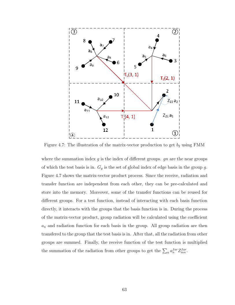
Figure 4.7: The illustration of the matrix-vector production to get b2 using FMM
where the summation index g is the index of different groups. gn are the near groups
of which the test basis is in. Gg is the set of global index of edge basis in the group g.
Figure 4.7 shows the matrix-vector product process. Since the receive, radiation and
transfer function are independent from each other, they can be pre-calculated and
store into the memory. Moreover, some of the transfer functions can be reused for
different groups. For a test function, instead of interacting with each basis function
directly, it interacts with the groups that the basis function is in. During the process
of the matrix-vector product, group radiation will be calculated using the coefficient
an and radiation function for each basis in the group. All group radiation are then
transfered to the group that the test basis is in. After that, all the radiation from other
groups are summed. Finally, the receive function of the test function is multiplied
the summation of the radiation from other groups to get the∑
n afarn Zfar
mn .
63

Near group
Far group
Self group
Figure 4.8: The illustration of near and far groups for a group
Figure 4.9: The illustration of octree from level 0 to level 2
4.7 Near and far groups
The figure 4.7 shows a general idea how group to group transfer is performed. In
the real situation, for each group, there are near groups (direct neighbors) and far
groups (non-direct neighbors) for this group. As shown in the figure 4.8 The near
groups for a group are the directly adjacent groups to it. And all the other groups
are the far groups of this group. The interaction between the group and near groups
besides with self group, are directly though explicitly calculated Zmn. FMM is only
used between a group and its far groups.
64

4.8 Multi-Level Fast Multipole Method
So far we only discussed one level of FMM. One of the disadvantages for that is the
number of transfer functions between groups grows exponentially as number of groups
grows. But if the number of groups is small, more near term of impedance matrix
has to be explicitly calculated. The fast multipole method can be easily extended to
multiple level by hierarchical octree group structures as show in figure 4.9. The top
level, level 0, is the big group which covers all the geometry. Evenly divied the big
group into 8 small groups for the level 1. The level 0 and level 1 are special levels.
The FMM can not apply for these two level. For level 0, all the basis (radiation
and receiving functions) are in the same group. And for level 1, groups are direct
neighbors. As discussed in the previous section, no transfer between direct neighbors.
From level 1, each small group is divided in to 8 sub-groups into level 2. The division
continues until to the finest groups. And usually the size of finest group is about one
fourth of wavelength. At the finest level, two groups which are far away from each
other do not have to interact with each other directly. It brought us to the terms
near neigbors and far neighbors.
4.9 Groups, near neighbors and far neighbors
Instead of just using near groups and far groups in one level FMM, MLFMM using
near neighbors and far neighbors. But berfore that, there are parent groups and child
groups between two adjacent levels. When a group is divided into 8 subgroups, that
group is the parent group of the subgroups. And the subgroups are the child groups
of the parent group. And these subgroups can be parents of their own sub-subgroups.
As demonstraed in the figure 4.10 , a group’s near and far neigbors are from subgroups
of its parent’s direct neighbor’s subgroups. Let us assume all these subgroups make a
set. Within this set, those are direct adjacent to a group are called the near neighbors
of that group. And the other groups in that set is called the far neigors. Besides this
set, there are a lot of other groups in the same level. But they are not dealt on this
level, but through aggregation, transfer in parent level, and deggregation, which will
65
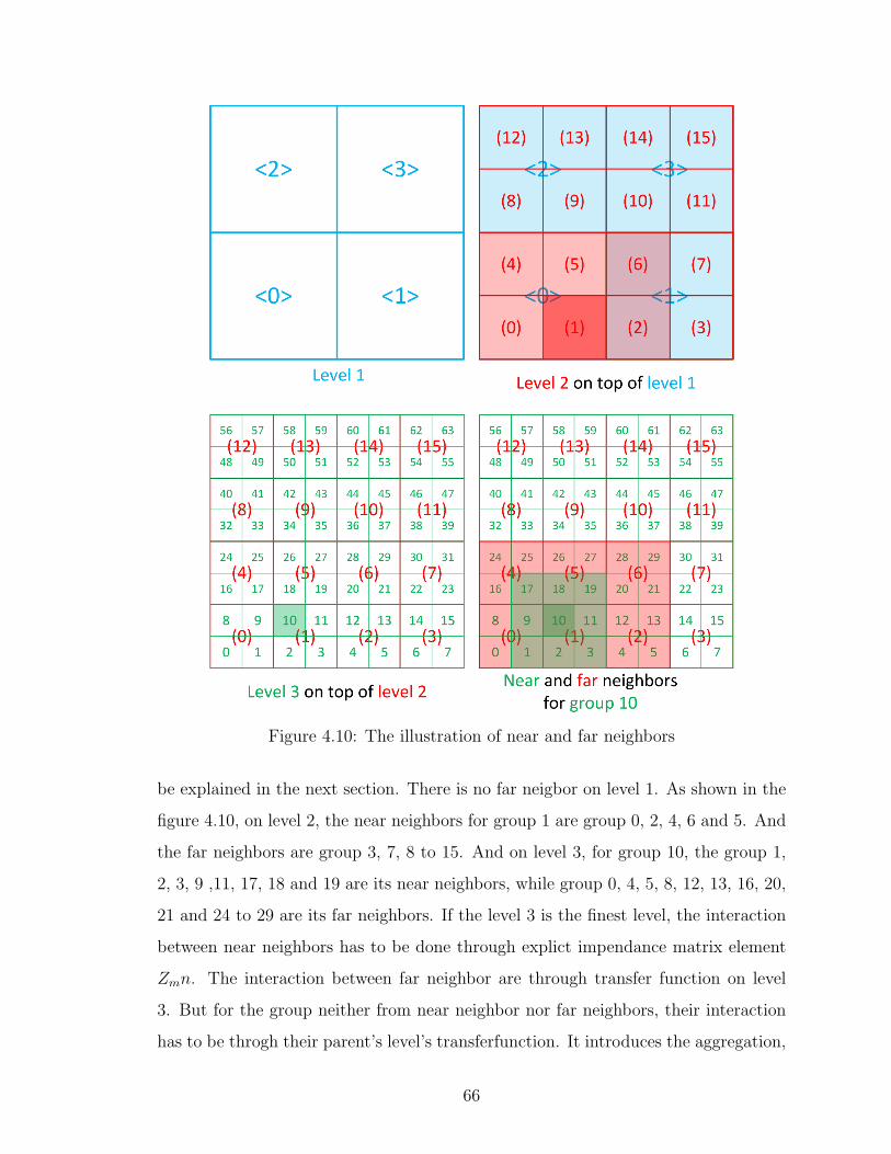
Figure 4.10: The illustration of near and far neighbors
be explained in the next section. There is no far neigbor on level 1. As shown in the
figure 4.10, on level 2, the near neighbors for group 1 are group 0, 2, 4, 6 and 5. And
the far neighbors are group 3, 7, 8 to 15. And on level 3, for group 10, the group 1,
2, 3, 9 ,11, 17, 18 and 19 are its near neighbors, while group 0, 4, 5, 8, 12, 13, 16, 20,
21 and 24 to 29 are its far neighbors. If the level 3 is the finest level, the interaction
between near neighbors has to be done through explict impendance matrix element
Zmn. The interaction between far neighbor are through transfer function on level
3. But for the group neither from near neighbor nor far neighbors, their interaction
has to be throgh their parent’s level’s transferfunction. It introduces the aggregation,
66

2
52
10
53
60 61
11
3
14
1
Figure 4.11: The illustration of aggregation, transfer and deaggregation
transfer and deaggregation for multi-level fast multipole method.
4.10 Aggregation, transfer and deaggregation
For two groups which are not near neigbors or far neighbors, their iteraction needs
help from their parent’s transfer functions. If their parent’s transfer function can still
not link them together, their parent’s parent’s transfer function may be needed and
so on. They can always link to each other throgh level 2 transfer functions at the
end. This brings the three stage of aggregation, transfer and deaggregation for far
away groups as shown in figure 4.11. For example, the group 10 interacts with group
60 on level 3. No direct transfer function on level 3 can do that. The need the level
2 transfer function from group 1 to group 14 on level 2.
67

0 1 20
2
0
0 1 2
3 4 5
3 4 5
6 7 8
6 7 8
12 13 14
91011
121314
151617
012
678
345
91011
121314
15 16 17
15 16 17
91011
12 13 14
9 10 11
9 10 11
121314
151617
678
345
012
678
345
012
151617
012
345
678
91011
121314
151617
Figure 4.12: The interpolation padding for θ and φ in Cartesian coordinate system
First, aggregate all the radiation function groups 2, 3, 10 and 11 on level 3 into
their parent group 1 on level 2. Then transfer the big group 1, to big group 14 throgh
level 2 transfere function. And deaggregate the group 14 into each small groups 52,
53, 60 and 61.
During the aggregation and deaggregation stage, the plane waves’ phase are
changed which needs to be included.
Rl−1an (k) = ejk0k·(r
lc−r
l−1c )Rl
an(k) (4.35)
Rl−1vm (k) = e−jk0k·(rlc−r
l−1c )Rl
vm(k) (4.36)
4.11 Interpolation on the sphere
Since different level has different Multipole L, which makes different sampling point
in different level. During the aggregation and de-aggregation of the results. Inter-
polation algorithm is needed to convert number of sample point from 2L1L1 of one
level to 2L2L2 of the other level. Lagrange polynomial interpolation is used for both
68

the θ and φ direction. One thing has to be notices is that both angles are periodical
function on the surface. Proper treatment needs to be done towards the end of each
angle. Mistake can be easily made during interpolation between different levels.
Figure 4.12 shows an example of L = 3 interpolation padding in Cartesian coor-
dinate. There are 18 data points. Be careful of which nodes will be used when the
interpolations is around the boundary of θ or φ.
4.12 Extra Space Storage for FMM and Multi-Level FMM
One of the advantages of using FMM is that only sparse impedance matrix needs
to be filled. But the FMM needs extra storage space for the radiation, receive and
transfer functions. For each function, it has to be stored in the form of a vector.
Suppose that N is the number of unknowns, then there are 4NL2 elements for the
radiation function and 4NL2 for the receiving function (2NL2 for θ direction and
2NL2 for φ direction). If M is the number of the transfer function, 2ML2 space
is needed for storing the transfer function. For one-level FMM, the larger number
of groups, the less number of impedance matrix element needs to be filled but the
more transfer process needs to be performed and more space is needed for storing
the transfer function. And the M is growing dramatically as the number of groups
increase. The FMM can reduce the matrix-vector product from O(N2) to O(N1.5)
[17].
The Multi-Level Fast Multipole Methods (MLFMM) extends the FMM from one
level to multi-levels. By doing that, it keeps the large number of small group at the
lowest level and maintains small interaction between groups.
Since the transfer functions are only dependent on the vector between two group
centers, they can be reused if the groups are separate appropriately. A Multi-Level
Fast Multipole Methods (MLFMM) [17] [30] was used to minimize the number of
total transfer function for large number of groups. Also the MLFMM can reduce
the matrix-vector product to O(N(logN)2). In MLFMM, unknowns are grouped in
cubes. It can minimize the maximum 316 transfer function for each level.
69
4.13 Storage of the Sparse Impedance Matrix
There are several ways to store the sparse matrix. One way to store the sparse matrix
is store the entry and both the row and column index together. But this not a efficient
way to store the sparse matrix. Here we will show a compressive way of storage in
our program.
First, all the finest group are numbered continuously, which each group has one
and more basis inside the group. For example, N finest group will be numbered from
0 to N-1. Second, all the edges which are associated with basis functions will be
reordered.
4.14 Numerical results
Our first test object is a sphere with radius 1m. It is meshed with 0.1m triangles.
The frequency is 0.3GHz. A comparison with MIE series is made as shown in figure
4.13. In this case, 0.25mm is used as the size of the finest group. The finest level is
level 3. Number of unknown 4050.
The second test object is a sphere with radius 1.9m. It is also meshed with 0.1m
triangles. The frequency is 0.3GHz. A comparison with MIE series is made as shown
in figure 4.14. 0.25mm is used as the size of the finest group. The finest level is level
4. And the number of unknown 15138.
The third test object is a 1 layer coated sphere with PEC sphere radius as 1.0m.
And the thickness of the coating is 0.1m with dielectric constant as εr = 2 − j1 It
is also meshed with 0.07m tetrahedrons. There are 2970 triangle mesh on the PEC
surface and 14633 tetrahedron for the volume. The frequency used is 0.3GHz. A
comparison with MIE series is made as shown in figure 4.15. 0.25mm is used as the
size of the finest group. The finest level is level 3. And the number of unknown 20671.
70

0 20 40 60 80 100 120 140 160 180elevation angle θ
−20
−15
−10
−5
0
5
10
15
20
25
RC
S (
dB
sm)
sp_1m
θθ
φφ
MIE θθ
MIE φφ
Figure 4.13: The Bi-Static RCS of PEC sphere with R = 1m solved with MLFMM
71

0 20 40 60 80 100 120 140 160 180elevation angle θ
−10
−5
0
5
10
15
20
25
30
35
RC
S (
dB
sm)
sp_1m9
θθ
φφ
MIE θθ
MIE φφ
Figure 4.14: The Bi-Static RCS of PEC sphere with R = 1.9m solved with MLFMM
72
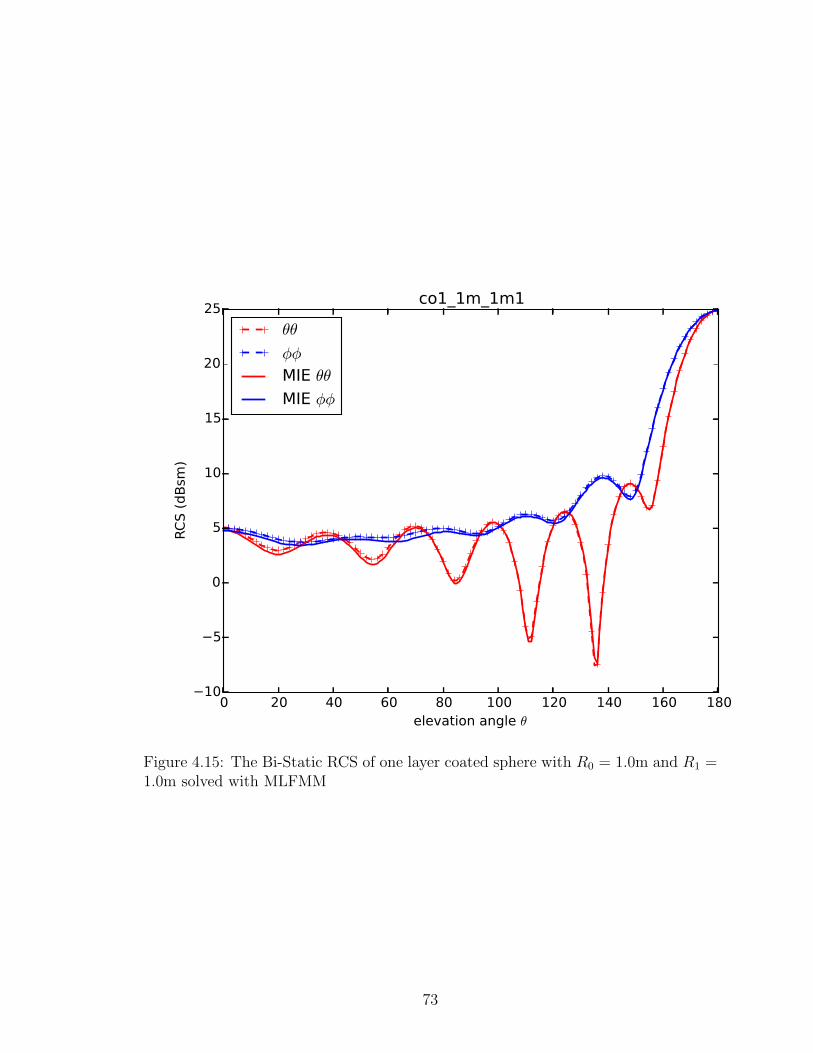
0 20 40 60 80 100 120 140 160 180elevation angle θ
−10
−5
0
5
10
15
20
25
RC
S (
dB
sm)
co1_1m_1m1
θθ
φφ
MIE θθ
MIE φφ
Figure 4.15: The Bi-Static RCS of one layer coated sphere with R0 = 1.0m and R1 =1.0m solved with MLFMM
73
Chapter 5
Solving Inverse Scattering Problems with Background Cancelling
5.1 Microwave Imaging
Radar imaging is an interdisciplinary technology. Formed from summation of weighted
scattering data of a range of frequencies and/or angles, a radar image was termed as
scattering brightness recommended in [8]. And radar imaging is one of technologies to
solve inverse scattering problems, which desires to get properties of the scatterer from
the scattered field measured outside the scatterer. It broadens humane’s sensory abil-
ity in viewing the world. Based on the different application, research can be found
in wave propagation, signal processing, and geoscience areas. One of the popular
radar image technologies is called Synthetic Aperture Radar (SAR) method. Mensa
in [21] has clearly presented two dimension high resolution radar imaging method
using focused synthetic aperture processing techniques. Based on the conclusion by
Mensa, a two dimensional image and its corresponding spectrum form a two dimen-
sional Fourier transform pair. This Fourier transformation pair relation applies only
to the cases that the transmitter and receiver are located at far field zone. This
kind of Fourier pair relationship can also be derived from diffraction tomography [6]
with simplifications. Based on the same imaging theory, near field imaging algorithm
can also be developed. But it requires two-dimensional integration. This image and
spectrum relationship allows us to use signal processing method to reconstruct the
two dimentional image. According to the signal processing theory, the resolution of
reconstructed image is limited by the band width of source frequency and measurable
angle. Multiple emitter location and signal parameter estimation (MUSIC) method
presented in [28] by Schmidt is used in super resolution radar imaging first by Oden-
dal and Barnard [23]. Its super resolution and its strength in high noise environment
received much attention in recent research. Recent application of MUSIC in two di-
74

mensional imaging can be found in [33] [35] [1]. The drawback of this algorithm is
that inversion of a matrix needs to be performed. This leads to time and memory
consuming issues. No real time imaging application has been found with this method
until now. Previous methods are focused on the signal processing point of view. In
scattering problems, the total field is related to the object by the integral equation
[6]
E(r) = Ei(r) +
∫
V
¯G0(r, r′) ·O(r′)E(r′)dr′ (5.1)
where E is the total field, Ei is the incident field, ¯G0 is dyadic green function. The
scatterer function O = k2(r′) − k2b contains information of the scatterer, where k
is the wave number in the scatterer and kb is the wave number in the background.
Nonlinear relationship exists between the total scattered field and scatterer function,
which is caused by the mutual interactions among the induced currents by the incident
wave. In the cases where only scattering field can be measured, equation 5.1 can be
rewritten as
Es(r) =
∫
V
¯G0(r, r′) ·O(r′)E(r′)dr′, (5.2)
where Es is the scattered filed.
For inverse problem, scatterer function needs to be solved by equation 5.1 or 5.2.
The nonlinear relationship between the scattered field and the object prevents us
from finding the solution easily. But problems can be vastly simplified by making
this nonlinear relationship approximately linear. One of such linearization conditions
is called the Born approximation. In first order Born approximation, we assumes that
the total field in the object is equal to the incident fiend. This is equivalent to the as-
sumption that the scattered field is much smaller than the incident field in the object
[6]. There are two unknowns in equation 5.1, the total field E(r) and object function
O(r). The idea of the Born iterative method is to alternatively fix one function,
and solve for the other. The limitations of the Born approximation is due to multiple
scattering effects of objects with high contrast in the dielectric permittivity. It is valid
for week scatters. So high-order imaging methods have been investigated. One of the
higher-order approximations is called distorted Born iterative method (DBIM). And
75

DBIM has been applied in Biomedical imaging, ground penetration imaging, ultra-
sound imaging technologies [16]. Different from BIM, the DBIM update the Green’s
function in each step corresponding to the object function. The penetrable ability of
electromagnetic wave into dielectric material gives widely application of radar imag-
ing in through wall imaging technologies. High resolution through wall images are
currently generated by using ultra wide band signals. Beam forming and refocus or
auto-focus algorithms have been researched to make adjustments for projection data
through solid material. Target displacement and ambiguities of reconstructed images
in the presence of a wall or other clutters can be refocused and sharpened by the idea
of match filter. Proposed by Dehmollaian and Sarabandi [10], compensation factor,
which is derived from transmissivity matrix, is used in the process of image recon-
struction. When parameters of a wall are not exactly known, reconstructed images
quality changes due to the variation of estimated transmissivity matrix. Square error
is used to determine the refocused image quality compared with the target image
without a wall. In practice, parameters of a wall are not exactly known. Imaging
through unknown walls is a tough issue when using beam forming and refocus algo-
rithms. A technique using two or more standoff distances of the imaging system form
the wall has been proposed by Wang and Amin [3], two image correction schemes was
also proposed. The first scheme is tracking the trajectories of target displacement
with different standoff distance and different estimated wall parameters. And target
position is determined as the trajectories crossover points. In the other scheme, an
image sequence is generated with different standoff distance and the same estimated
wall parameters, and then an imaging-focusing metric is used to determine the tar-
gets’ position. But as Baranoski wrote in [3], ”tomographic approaches are well suited
for shadowing and attenuation effects, but do not account for multipath and Bragg
scattering”. Complex phenomenology occurs when electromagnetic waves penetrate
a wall. Inspired by volume integral equations, consider the background and the object
as different scattering sources, by ignoring the interaction between two sources, the
total field can be written as
Et = Ei + Esbg + Es
Obj (5.3)
76

Figure 5.1: Mono-static and Bi-static imaging geometries
where Esbg is the scattered field due to the background and Es
Obj is the scattered
field of the objects. In the cases that background scattering is high, the objects may
be undetectable. In cases when the background properties are known, it is possible
numerically calculate the scattered field (of the same source) by background only.
If the background scattered field is subtracted from the total measured field, it is
expected that better reconstruction of the objects could be achieved.
5.2 Introduction of Focused Synthetic Aperture Processing
Considering the problem of obtaining a two-dimensional (2D) image of an object
by processing reflected signals using a source and a receiver located in the cross-
section plane. The cross section is characterized by a two-dimensional distribution
of scattering centers, denoted by g(x, y), which is termed the reflectivity density
function. The mono-static and bi-static imaging geometries are shown in 5.1. The
Tx is denoted as a transmitter, while Rx is denoted as a receiver. For mono-static
case, the Tx and Rx is at the same place, which is denoted as Tx/Rx. The observation
distance is assumed to be sufficiently greater than the object extent so that iso-range
contours can be assumed to be straight lines normal to the line-of-sight. The objective
is to obtain a reconstruction of g(x, y) by processing the received signals from various
77
aspect angles [21].
We consider an attributed scattering center model as a representation of object
backscatter in our imagery. At high frequencies, the radar backscatter from an object
is well-approximated as the sum of response from individual scattering centers on the
object. In this case, the reconstructed images consist of discrete individual points.
Another approximation in this imaging process is that there is no interaction among
those scattering centers.
According to the imaging geometries shown in figure 5.1, the general format of
the received signal caused by a single scatter point at (x, y) is given by
Esca = Eincg(x, y)e−j2π(rt+rr)/λ, (5.4)
where Esca is the scattered electric field intensity, Einc is incident electric field inten-
sity, g(x, y) is the reflectivity density, rt is the distance between the transmitter and
the scatter point and rr is the distance between the receiver and the scatter point; is
the wave length. In mono-static cases, we have r = rt = rr. The g(x, y) is a complex
number. Its magnitude and phase represent the attenuation and the phase shift of
the incident field. It is the electric property of the object itself. The received signal
at certain angle can be expressed as the two dimension integration of scattered field
caused by each individual scatter point. Assuming the incident field is plane wave
with magnitude one, the received field can be written as
G(f, θt, θr) =
∫∫
D
g(x, y)e−j2π(rt+rr)/λdxdy, (5.5)
where the D is the extent of the scatterers. For far field, by substituting
rt + rr = Rt − (x cos θt + y sin θt) +Rr − (x cos θr + y sin θr), (5.6)
applying trigonometric identities and multiply on both side with focus phase delay
e−j2π(Rt+Rr)
λ , the equation 5.5 can be rewritten as
G(f, θt, θr) =
∫∫
D
g(x, y)ej4πλ[x cos(
θt+θr2
) cos(θt−θr
2)+y sin(
θt+θr2
) cos(θt−θr
2)]dxdy (5.7)
78
Equation 5.7 gives a relationship between the image and the received signals in bi-
static case. Defining
Xbi =2f
ccos(
β
2) cos(
θt + θr2
), (5.8)
Ybi =2f
ccos(
β
2) sin(
θt + θr2
), (5.9)
and
G(X, Y ) = G(f, θt, θr) (5.10)
where c is the speed of light in free space, and β = θr − θt is the bi-static angle. The
equation 5.7 can be rewritten as
G(X, Y ) =
∫∫
D
g(x, y)ej2π(Xx+Y y)dxdy (5.11)
In mono-static cases, applying θ = θt = θr and r = rt = rr, the expression 5.7 can
be further simplified as,
G(f, θ) =
∫∫
D
g(x, y)e−j 4πλ(x cos θ+y sin θ)dxdy (5.12)
The same equation 5.11 can be derived by defining
Xmo =2f
ccos(θ) (5.13)
Ymo =2f
csin(θ) (5.14)
and
G(X, Y ) = G(f, θ) (5.15)
The equation 5.11 shows a Fourier transformation relationship between theG(X, Y )
and the spacial distribution of reflectivity g(x, y) [21]. So g(x, y) can be obtained by
doing the Fourier transformation by
g(x, y) =
∞∫∫
−∞
G(X, Y )e−j2π(Xx+Y y)dXdY (5.16)
79

Figure 5.2: The data sampling pattern in mono-static cases
Figure 5.3: The data sampling pattern in bi-static cases
5.3 Interpolation
Numerical evaluation of g(x, y) in equation 5.16 can be obtained by doing 2D Fast
Fourier Transformation(2D-FFT). In that case, the X, Y needs to be sampled in
uniform grid in X-Y plane. But in practice, measurement results are obtained from
different frequency and incident or receiving angles. We will show the pattern of the
sampled (X, Y ) points for mono-static and bi-static case. Then we will show the
interpolation schemes to transfer the patterns to a 2D uniform grid distribution for
the 2D-FFT.
Figure 5.2 shows evenly angle sampled single frequency and multiple frequencies
80

Figure 5.4: The sampling configuration and scheme
measured data samples in mono-static cases, while figure 5.3 shows measured data
samples in bi-static cases in different situations.
In figure 5.2, (a) shows data samples by the angle evenly spaced single frequency
case, while (b) shows data sample by multi-frequency case. The radius of each single
circle, which is shown with dash lines, is ρ = 2f/c. Note that the measured data
does not necessary cover whole rings. The coverage dependents on the coverage of
incident and observation angle.
In figure 5.3, (a) shows data samples with fixed transmitter evenly spaced bi-static
angle of single frequency source. (b) shows two transmission angle evenly spaced
bi-static angle with single frequency. (c) shows multi-frequencies extension for (a).
Another case is rotating object with fixed both transmitter and receiver, samples on
a circle.
Thus, to implement 2D FFT, interpolation schemes are needed to obtain evenly
data samples in X and Y direction. Here we propose simple and easy-to-implement
mapping schemes. Since the sample patterns are different for mono-static and bi-
static case, we will first discuss interpolation scheme for mono-static cases followed
by interpolation scheme for bi-static cases.
Mono-static interpolation scheme
Consider the fact that data samples are obtained at different frequencies and different
angles, instead of doing 2D interpolation on X −Y plane, we map the grid on X −Y
81

plane to f−θ plane first and implement 2D interpolation on f−θ plane. The mapping
algorithm is based on equation 5.13 and 5.14. Those two equations yield 5.17 and
5.18
f =c√
X2mo + Y 2
mo
2(5.17)
θ = tan−1 (Ymo/Xmo) (5.18)
Figure 5.4 shows the interpolation scheme which takes the following steps.
1. Determine the region of samples and the sample density on X−Y plane (which
is the number of sampling points per unit area).
2. Select evenly sampled grids on X − Y plane whose area covers original sample
area but in rectangular shape. New sample density can be set the same as
original ones, or according to extent of the image area.
3. For each new sample, map the coordinates (Xi, Yi) on X − Y plane to (fi, θi)
on f − θ plane by using equations 5.13 and 5.14.
4. Choose a 2D interpolation method to determine the electric field on each point
(fi, θi). Interpolations are performed on real and imaginary part separately.
5. Apply 2D IFFT on the equally spaced samples to get the reconstruction of the
image.
As can be seen from the method, it requires no evenly spaced frequency samples
or evenly spaced angle samples.
Bi-static interpolation scheme
As shown in mono-static interpolation scheme, the same interpolation concept is used
in bi-static cases. In doing step 3, instead of mapping grids on X − Y plane to f − θ
plane, we map those grids on X − Y plane to θt − θr plane by using algorithm
θr = α± cos−1
(√
X2 + Y 2
2
)
(5.19)
82
θt = α∓ cos−1
(√
X2 + Y 2
2
)
(5.20)
where X = Xcf
,Y = Y cf
and α = tan−1( YX). Equation 5.19 and 5.20 are derived from
equation 5.8 and 5.9. In this case, 2D interpolation should be performed on θt − θr
plane.
5.4 Resolution analysis
The object in interest with the reflectivity density g(x, y) is usually a space limited
function. Based on Fourier transform theory, its corresponding spectrum G(X, Y )
is a function with X and Y in infinite range. But practically, the received electric
field is usually in a limited bandwidth and the transmission angle and receiving angle
can not always reach to 360 degrees. For all of those limitations, the received signal
G(X, Y ) is a truncated G(X, Y ) by different windows functions in two dimension.
G(X, Y ) = W (X, Y )G(X, Y ) (5.21)
The 2D Fourier transformation of the windows function, which is called the point-
spread function, has been discussed and explained in [21]. The 2D annular shape
window and its corresponding point spread function can be represented by
H2D(ρ) =
1, ρmin < ρ < ρmax
0, otherwise
(5.22)
and
h2D(r) = ρmaxJ1(2πρmaxr)
r− ρmin
J1(2πρminr)
r(5.23)
where J1 is the first order Bessel function.
5.5 Numerical results
The first case is a PEC sphere with radius of 0.2m at (0.1, 0, 0) in cartision coordinate
system. The frequency 0.3GHz is used. The sweeping angle is φ. 91 sampling points
are used from [0, 2π). The imaging is shown in figure 5.5.
83
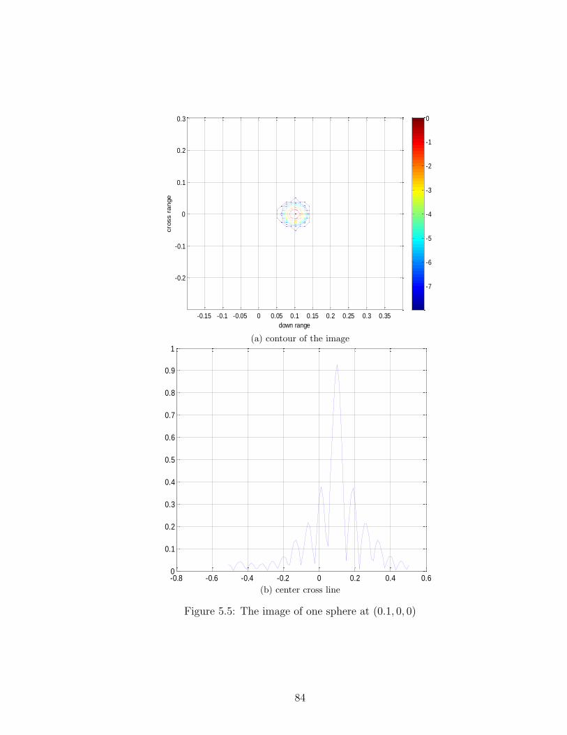
down range
cro
ss r
an
ge
-0.15 -0.1 -0.05 0 0.05 0.1 0.15 0.2 0.25 0.3 0.35
-0.2
-0.1
0
0.1
0.2
0.3
-7
-6
-5
-4
-3
-2
-1
0
(a) contour of the image
-0.8 -0.6 -0.4 -0.2 0 0.2 0.4 0.60
0.1
0.2
0.3
0.4
0.5
0.6
0.7
0.8
0.9
1
(b) center cross line
Figure 5.5: The image of one sphere at (0.1, 0, 0)
84

down range
cros
s ra
nge
-0.2 -0.1 0 0.1 0.2-0.2
-0.15
-0.1
-0.05
0
0.05
0.1
0.15
0.2
-7
-6
-5
-4
-3
-2
-1
0
(a) contour of the image
-0.8 -0.6 -0.4 -0.2 0 0.2 0.4 0.60
0.1
0.2
0.3
0.4
0.5
0.6
0.7
0.8
0.9
1
(b) center cross line
Figure 5.6: The image of two spheres at (−0.1, 0, 0) and (0.1, 0, 0)
85
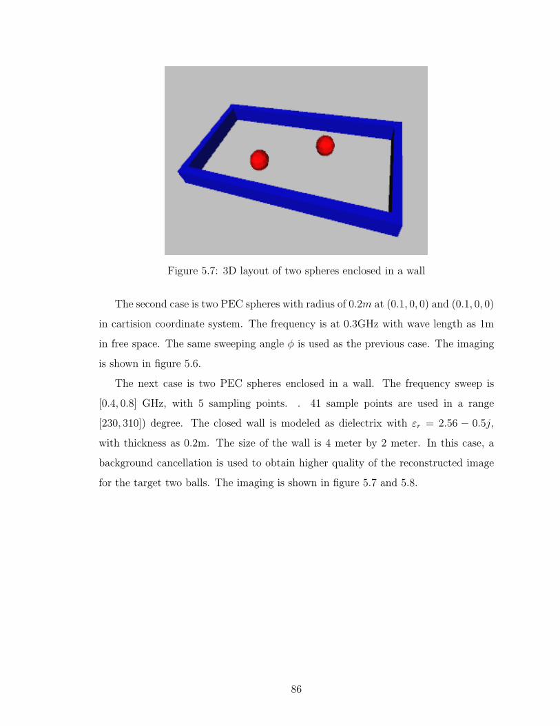
Figure 5.7: 3D layout of two spheres enclosed in a wall
The second case is two PEC spheres with radius of 0.2m at (0.1, 0, 0) and (0.1, 0, 0)
in cartision coordinate system. The frequency is at 0.3GHz with wave length as 1m
in free space. The same sweeping angle φ is used as the previous case. The imaging
is shown in figure 5.6.
The next case is two PEC spheres enclosed in a wall. The frequency sweep is
[0.4, 0.8] GHz, with 5 sampling points. . 41 sample points are used in a range
[230, 310]) degree. The closed wall is modeled as dielectrix with εr = 2.56 − 0.5j,
with thickness as 0.2m. The size of the wall is 4 meter by 2 meter. In this case, a
background cancellation is used to obtain higher quality of the reconstructed image
for the target two balls. The imaging is shown in figure 5.7 and 5.8.
86
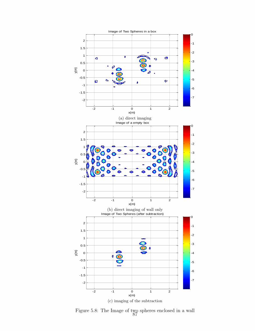
x(m)
y(m
)
Image of Two Spheres in a box
-2 -1 0 1 2
-2
-1.5
-1
-0.5
0
0.5
1
1.5
2
-7
-6
-5
-4
-3
-2
-1
0
(a) direct imaging
x(m)
y(m
)
Image of a empty box
-2 -1 0 1 2
-2
-1.5
-1
-0.5
0
0.5
1
1.5
2
-7
-6
-5
-4
-3
-2
-1
0
(b) direct imaging of wall only
x(m)
y(m
)
Image of Two Spheres (after subtraction)
-2 -1 0 1 2
-2
-1.5
-1
-0.5
0
0.5
1
1.5
2
-7
-6
-5
-4
-3
-2
-1
0
(c) imaging of the subtraction
Figure 5.8: The Image of two spheres enclosed in a wall87

Chapter 6
Conclusion and future work
Based on the research and the result we have obtained, it shows the feasibility of
forming integral equations for complex objects by using hybrid divergence-conforming
basis function and curl-conforming basis functions. As far as we know, this is the
first time to put them together and also implemented with MLFMM.
With the same tetrahedron mesh, less number of unknown is expected when curl-
conforming basis function is used compare to the divergence-conforming basis function
is used. This is based on the fact that the number of the edges is less than the number
of the faces for a tetrahedron mesh. Dr. Lu has published on [19] that the condition
number of the impedance matrix is comparable between those two kinds of basis
functions when the number of unknowns is comparable.
Future work on VSIE involves speed up the matrix filling part and solving part
by massive parallel computation technology.
By using the calculated near and far field of models, a microwave imaging can
be improved as regard to the resolution of the image. As demostrated in the exam-
ples, hiden object, which due to the low resultion can be revealed if the background
substraction technique is used. The future work on this part involves more study
on how applicable this techonolgy into real measured data. And also more study
should be focused when the object is not well modeld, such as the thickness of walls
is not accurately modeled and the permittivity is not exactly know. Further more,
higher resolution imaging techique such as MUSIC should be used for better imaging
together with this backgroud cancelling technique.
88

Appendix A: Numerical Integration of Singular Integrands
Singularity of the Green’s Function
The power of the Green’s function converting the electric current directly into electric
field makes no grid error in integral equation methods in solving EM problems. The
Green’s function in free space is
G0(r, r′) =
1
4πRe−jk0R =
1
4π[R−1 cos(k0R)− jR−1 sin(k0R)], (6.1)
where
R = |r− r′| =√
(x− x′)2 + (y − y′)2 + (z − z′)2. (6.2)
Since
limR→0
R−1 sin(k0R) = k0, (6.3)
0.00 0.05 0.10 0.15 0.2010-2
10-1
100
101
102
Re(G0 )/k0
1/(4πR)/k0
0.00 0.05 0.10 0.15 0.20R/λ
−0.08
−0.07
−0.06
−0.05
−0.04
−0.03
−0.02
−0.01
0.00
[Re(G0 )−1/(4πR)]/k0
Im(G0 )/k0
Figure 6.1: The illustration of the singularity in G0
89

0.00 0.05 0.10 0.15 0.2010-2
10-1
100
101
102
103
104
|Re(∇G0 )|/k 20
1/(4πR2 )/k 20
0.00 0.05 0.10 0.15 0.20R/λ
−0.04
−0.03
−0.02
−0.01
0.00
0.01
0.02
0.03
[Re(|∇G0 |)−1/(4πR2 )]/k 20
Im(|∇G0 |)/k 20
Figure 6.2: The illustration of the singularity in ∇G0
there is no singularity of the imaginary part of the Green’s function. For the real
part, we have
limR→0
(R−1 cos(k0R)−R−1) = limR→0
(−1
2k20R) = 0. (6.4)
So G0 has the same singularity of 14πR
when R approaches to zero. Figure 6.1 shows
the difference between Re(G0) and1
4πRat 1.0 GHz. After the singular extraction of
the Green’s function on the real part, the nonsingular part of the Green’s function
can be approximate get by doing series expansion
G0 −1
4πR≈ 1
4π
[
−k20R
2+ j(
k30R
2
6− k0)
]
. (6.5)
The figure also shows the nonsingular part of the Green’s function at 1.0 GHz. Al-
though the results shown in the figure 6.1 is at 1.0 GHz, it can be very stable for large
range of frequencies. Another thing should be noted here is that the wave length is
in free space.
We will examine the singularity of the gradient of the Green’s function. The
90
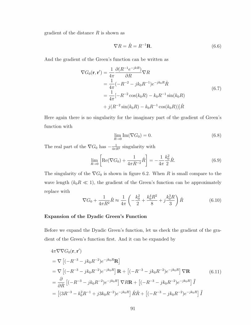
gradient of the distance R is shown as
∇R = R = R−1R. (6.6)
And the gradient of the Green’s function can be written as
∇G0(r, r′) =
1
4π
∂(R−1e−jkR)
∂R∇R
=1
4π(−R−2 − jk0R
−1)e−jk0RR
=1
4π[−R−2 cos(k0R)− k0R
−1 sin(k0R)
+ j(R−2 sin(k0R)− k0R−1 cos(k0R))]R
(6.7)
Here again there is no singularity for the imaginary part of the gradient of Green’s
function with
limR→0
Im(∇G0) = 0. (6.8)
The real part of the ∇G0 has − 14πR2 singularity with
limR→0
[
Re(∇G0) +1
4πR−2R
]
= − 1
4π
k20
2R. (6.9)
The singularity of the ∇G0 is shown in figure 6.2. When R is small compare to the
wave length (k0R ≪ 1), the gradient of the Green’s function can be approximately
replace with
∇G0 +1
4πR2R ≈ 1
4π
(
−k20
2+
k40R
2
8+ j
k30R
3
)
R (6.10)
Expansion of the Dyadic Green’s Function
Before we expand the Dyadic Green’s function, let us check the gradient of the gra-
dient of the Green’s function first. And it can be expanded by
4π∇∇G0(r, r′)
= ∇[
(−R−3 − jk0R−2)e−jk0RR
]
= ∇[
(−R−3 − jk0R−2)e−jk0R
]
R+[
(−R−3 − jk0R−2)e−jk0R
]
∇R
=∂
∂R
[
(−R−3 − jk0R−2)e−jk0R
]
∇RR+[
(−R−3 − jk0R−2)e−jk0R
] ¯I
=[
(3R−3 − k20R
−1 + j3k0R−2)e−jk0R
]
RR +[
(−R−3 − jk0R−2)e−jk0R
] ¯I
(6.11)
91

so the Dyadic Green’s function can be written as
4π ¯G0 = 4π
(
¯I +1
k20
∇∇)
G0 = 4πG0¯I +
1
k20
4π∇∇G0
=[
1− (k0R)−2 − j(k0R)−1]
R−1e−jk0R ¯I
+[
3(k0R)−2 − 1 + j3(k0R)−1]
R−1e−jk0RRR
(6.12)
By substituting e−jk0R = cos(k0R)− j sin(k0R) into equation 6.12, the real part and
the imaginary part of the Dyadic Green’s function can be written as
Re( ¯G0) =1
4π
[
cos(k0R)− (k0R)−1 sin(k0R)− (k0R)−2 cos(k0R)]
R−1 ¯I
+1
4π
[
− cos(k0R) + 3(k0R)−1 sin(k0R) + 3(k0R)−2 cos(k0R)]
R−1RR(6.13)
and
Im( ¯G0) =1
4π
[
− sin(k0R)− (k0R)−1 cos(k0R) + (k0R)−2 sin(k0R)]
R−1 ¯I
+1
4π
[
sin(k0R) + 3(k0R)−1 cos(k0R)− 3(k0R)−2 sin(k0R)]
R−1RR.(6.14)
Similarly, it is easy to prove that there is no singularity of the imaginary part of the
Dyadic Green’s function and
limR→0
Im( ¯G0) =1
4πk0(RR− ¯I). (6.15)
And the real part of the Dyadic Green’s function has singularity part as
1
4πk20[(3R
−3 + 2R−1)RR−R−1 ¯I]. (6.16)
Analytic Solution of Triangle
Consider a singular integration on a triangle,
f(r) =
∫
1
|r− r′|dr′ (6.17)
where r is inside the triangle as shown in figure 6.3. The domain of the integration
can be divided into three small triangles (0, 1 and 2). The integral is the summation
of the integral on the three triangles. We will take a look at the small triangle formed
by r, r1 and r2. Perform the integration in a polar coordinate system, we have
f0(r) =
∫ θ2
θ1
∫ d/ cos θ
0
1
ρρdρdθ = ln
| sec θ2 + tan θ2|| sec θ1 + tan θ1|
= ln|R2 + y2||R1 + y1|
(6.18)
92

Figure 6.3: The singular integral on a triangle
where θ1 and θ2 are in the range of (−π, π]. The θ1 and θ2 and be calculated by
θ1 = atan2(y1, d), θ2 = atan2(y2, d), where y1 and y2 is the y coordinate of point
r1, r2 at the new coordinate system respectively (y1 should be a negative number as
shown in the figure). R1 and R2 are the distance from the point r to the points r1
and r2 respectively. In the cases that r is on one of the edge of the triangle, only
two integral needs to be evaluated. The other one should be avoid. Also in the cases
that the r is at the one of the vertices of the triangle, only one integral needs to be
evaluate. Both of the other two should be avoid. Because the R1 + y1 can be 0 for
those avoided evaluations.
Numerical quadrature with singular integrand
For integral method, one of the issue that cannot be avoid is integration with sin-
gular kernels. Depends on the equation chosen as the EFIE or MFIE, the order of
the singularity can be different. A kernel with 1/R2 is hyper singular for a volume
integration. The singularity is a challenge for numerical integrations. And the in-
tegration of kernel R/R2 makes the numerical quadrature even harder in practice.
The typical way of handling this issue is by performing Duffy transformation. But
93

Figure 6.4: Duffy transformation for a tetrahedron with singularity at a vertex
by doing Duffy transformation, the radius and the angle are distorted, which in turn
makes result converge slowly for high singular kernels.
We have developed a simple and more intuitive method for numerical integrations
with high order singular kernels. This method performs the integration in spherical
coordinates. Therefore, the radius and angle information are kept. In the spherical
coordinate, the singularity is naturally eliminated. But the problem changes to how
to model a Cartesian curvilinear volume in a spherical coordinates. In this method,
by doing proper coordinate transformation, we can mesh a tetrahedron in a spherical
coordinate with small number of cells. For each cell, the analytical results can be
calculated for different type of kernels with controllable error. In the method, the
vertices and the surface of the tetrahedron are considered carefully to reduce the error
which are introduced by the mesh itself. Although this method is implemented for
integration in tetrahedron, but it can be apply to any linear volume shapes, such as
cubes and prisms.
The proposed method is very intuitive and easy to be implemented. Numerical
results show good converge rate when the number of cells is increased. In the paper,
we will present both the advantages and disadvantages of this method compare to
the traditional Duffy transformation method. Also presented is how to apply this
method to solve volume and surface integral equations.
Duffy transformation for a tetrahedron with a singularity at vertex
Numerical evaluation of multidimensional integrals of singular function can be trou-
blesome. Duffy transformation is to transform strong singularity at a point to a softer
94
singularity on a surface. And by doing the transformation, Gauss quadrature rule
can be used for each dimension of a cube. The original transform presented in [11]
transform integration in a pyramid into a cube. Here we will show how to transform
a tetrahedron into a cube.
Assume that the singularity occurs at the vertex 0 of a tetrahedron as shown in
figure 6.4. This is the case when the test point is at vertex 0. The singularity is due
to the green’s functions or its derivative. Here we assume the singularity is 1/R2,
where R is the distance from the point inside the tetrahedron to the vertex 0. By
interpolate the original Cartesian coordinate by the local simplex coordinates u, v, w
as
r = r0 + (r1 − r0)u+ (r2 − r1)v + (r3 − r2)w (6.19)
. The original integration can be transfered into the integration in the simplex coor-
dinate as∫
V
f(R)
R2dV =
√g
∫ 1
0
∫ u
0
∫ v
0
f(R)
R2dwdvdu (6.20)
, where√g is the Jacobian of the original tetrahedron. It equals six time of the
volume for tetrahedrons. The f(R) in 6.20 is a non-singular function and R can be
represented by
R = |r− r0| = |(r1 − r0)u+ (r2 − r1)v + (r3 − r2)w| (6.21)
Then another transformation is performed to transfer the integration in the tetrahe-
dron into a volume integration in a cube.
v = uv1, dv = udv1 (6.22)
w = vw1, dw = uv1dw1 (6.23)
And the
R2 = |u[(r1 − r0) + (r2 − r1)v1 + (r3 − r2)v1w1]|2
= u2|[(r1 − r0) + (r2 − r1)v1 + (r3 − r2)v1w1]|2
= u2|R1|2(6.24)
95
The R1 is used as a temporary variable in equation 6.24. It is easy to see that for
v1 ∈ [0, 1] and w1 ∈ [0, 1], R1 is always greater than zero. A simple proof is that to
make R1 = 0 is to validate the following equation.
r0 − r1 = −v1[(r2 − r1) + (r3 − r2)w1] (6.25)
From the equation, we can derive that the vector r1 − r0 is parallel to vector
(r2 − r1) + (r3 − r2)w1. The vector r1 − r0 is the vector point from vertex 0 to vertex
1, while the vector (r2 − r1) + (r3 − r2)w1 is the vector point from vertex 1 to the
point on the edge 2-3. We can see on the figure 6.4 the two vectors can not parallel
to each other for all w1.
And the singular integral becomes∫ 1
0
∫ u
0
∫ v
0
f(R)
R2dwdvdu =
∫ 1
0
∫ 1
0
∫ 1
0
f(R)
R2u2v1dw1dv1du
=
∫ 1
0
∫ 1
0
∫ 1
0
f(R)
|R1|2v1dw1dv1du
(6.26)
It can been seen that there is no singularity on the new integrand in equation 6.26.
Therefore, quadrature rules can be used for each dimension on the integration over
the cube.
Singular Integration in Spherical Coordinate
The singular integration can be handled in the sphecial coordinate. Consider about
a volume integration for a tetrahedron with one of its vertice at the origin, and one
of its edge is along the z axis as show in figure 6.5,∫∫∫
1
r2dxdydz (6.27)
where r =√
x2 + y2 + z2, the integrand is singular at the origin. In the spherical
coordinate, the previous integration becomes∫∫∫
sin θdθdφdr (6.28)
It can be seen that the sigularity is automatically removed in spherical coordinate
system. But the problem becomes how a tetrahedron is represented in spherical
96

1
2
3
o yx
z
(a) the whole tetrahedron
1' 2'
3
o yx
z
(b) a slice of tethrahedron
o yx
z
ab
cd
(c) a cell of tethrahedron
o yx
z
a
bc
(d) a half cell of tethrahedron
Figure 6.5: Singular integration in spherical coordinate system
coordinate. Below we show how to solve it appoximatly through mesh the tetrahedron
in spherical coordinate.
It is done by meshing the tetrahedron in azimuth angle and elevation angle, which
are represented by φ and θ. The range of θ is always starts from zero since the 0-3
edege is along the z axis. And its upper limits is determined by the vetices 1 and
2. The range of the φ is only determined by the vertices 1 and 2. They are in math
format
θ ∈ [0,max(θ1, θ2)] (6.29)
and
φ ∈ [φ1, φ2]. (6.30)
Please note that we assume that φ2 is always greater than φ1. 2π compensation may
be needed for φ2 in real cases considering that φ is periodic. It can be noted that
97

the facet 0-1-3 share the same azimuth angle φ1, while the facet 0-2-3 share the same
azimuth angle φ2. That will reduce the mesh error on the two facets. While the other
two facets 1-2-3 and 0-1-2 share neither the angle θ nor the angle φ. Mesh error exists
on both facets. In that case, approximation and mathmatic treatment are need for
better representaton.
First, the original tetrahedron is divided into slices of sub-tetrhahedrons. Each
sub-tetrahedron with azimuth angle range of ∆φ, as shown in figure 6.5. Then divide
the subtetrahedron in elevation angle ∆θ. For a normal cell, we have the integration
∫ r1
0
dr
∫ θ2
θ1
sin θdθ
∫ φ2
φ1
dφ = −r1 (cos θ2 − cos θ1) (φ2 − φ1) (6.31)
As you may noted, the outer surface of each cells away from the radius direction
is not a ideal in spherical coordinate. The outer surface is not spherical, but flat. The
four outer nodes may have different raidus. Assume their radius are ra, rb, rc and rd.
A simple way to approximate that is to get a average, that is
r1 = 0.25 (ra + rb + rc + rd) (6.32)
The smaller of ∆φ and ∆θ, the more accurate of the approximation. As they approach
to zero, the numerical result get infinit close to the exact result. This is not the best
way for the approximation, but is a practical way and easy to implement. If there are
two spherical surface can include the flat surface with ∆r, the error should no larger
than ∆r/r1. This is due to the the linear result change with respect to the radius
direction.
For the boundary on surface 0-1-2, there are half cells as shown in figure 6.5. In
that case, coefficient of 0.5 is multiplied on the integration of equation 6.31. And the
r1 is calculated by
r1 = 0.25 (2ra + rb + rc) (6.33)
Application of Solving Volume integration
As mentioned at the begining, the singular part of integrand for the volume integral
equations is not simple as 1/r2. One of the singular integrand in the previous chapters
98

is∫∫∫
r
r2Lidxdydz (6.34)
where Li, i = 0, 1, 2, 3 is the simplex coordinate in the tetrahedron. But before we
doing that, there are simple components of the integration needs to be calculated.
Let us define the simple integration first
I0 =
∫ r1
0
dr = r1 (6.35)
I1 =
∫ r1
0
rdr = 0.5r21 (6.36)
I2 =
∫ θ2
θ1
sin2 θdθ = 0.5 (θ2 − θ1)− 0.25 (sin 2θ2 − sin 2θ1) (6.37)
I3 =
∫ θ2
θ1
sin3 θdθ = −0.75 (cos θ2 − cos θ1) + (cos 3θ2 − cos 3θ1) /12 (6.38)
I4 =
∫ θ2
θ1
sin θ cos θdθ = −0.25 (cos 2θ2 − cos 2θ1) (6.39)
I5 =
∫ θ2
θ1
sin2 θ cos θdθ = 0.25 (sin θ2 − sin θ1)− (sin 3θ2 − sin 3θ1) /12 (6.40)
I6 =
∫ θ2
θ1
sin θ cos2 θdθ = 0.25 (cos θ1 − cos θ2)− (cos 3θ2 − cos 3θ1) /12(6.41)
I7 =
∫ φ2
φ1
dφ = φ2 − φ1 (6.42)
I8 =
∫ φ2
φ1
sinφdφ = − (cosφ2 − cosφ1) (6.43)
I9 =
∫ φ2
φ1
cosφdφ = (sinφ2 − sinφ1) (6.44)
I10 =
∫ φ2
φ1
sinφ cosφdφ = −0.5 (cos 2φ2 − cos 2φ1) (6.45)
I11 =
∫ φ2
φ1
sin2 φdφ = 0.5 (φ2 − φ1)− 0.25 (sin 2φ2 − sin 2φ1) (6.46)
I12 =
∫ φ2
φ1
cos2 φdφ = 0.5 (φ2 − φ1) + 0.25 (sin 2φ2 − sin 2φ1) (6.47)
99

And
Ix =
∫∫∫
x
r3dxdydz =
∫∫∫
sin θ cosφ
r2dxdydz = I0I2I9 (6.48)
Iy =
∫∫∫
y
r3dxdydz =
∫∫∫
sin θ sinφ
r2dxdydz = I0I2I8 (6.49)
Iz =
∫∫∫
z
r3dxdydz =
∫∫∫
cos θ
r2dxdydz = I0I4I7 (6.50)
Ixy =
∫∫∫
xy
r3dxdydz =
∫∫∫
sin2 θ sinφ cosφ
rdxdydz = I1I3I10 (6.51)
Ixz =
∫∫∫
xz
r3dxdydz =
∫∫∫
sin θ cos θ cosφ
rdxdydz = I1I5I9 (6.52)
Iyz =
∫∫∫
yz
r3dxdydz =
∫∫∫
sin θ cos θ sinφ
rdxdydz = I1I5I8 (6.53)
Ixx =
∫∫∫
x2
r3dxdydz =
∫∫∫
sin2 θ cos2 φ
rdxdydz = I1I3I12 (6.54)
Iyy =
∫∫∫
y2
r3dxdydz =
∫∫∫
sin2 θ sin2 φ
rdxdydz = I1I3I11 (6.55)
Izz =
∫∫∫
z2
r3dxdydz =
∫∫∫
cos2 θ
rdxdydz = I1I6I7 (6.56)
So we can easily get the integration of∫∫∫
r
r2dxdydz = xIx + yIy + zIz. (6.57)
Since the Li is the simplex coordinate in the tetrahedron, it can be represented by
Li = aix+ biy + ciz + di (6.58)
where ai, bi, ci and di are constant, which are determined by the coordinates of the
four vertices of the tetrahedron. So
∫∫∫
r
r2Lidxdydz = x (aiIxx + biIxy + ciIxz + diIx)
+ y (aiIxy + biIyy + ciIyz + diIy)
+ z (aiIxz + biIyz + ciIzz + diIy) (6.59)
To determine the ai, bi, ci and di, assuming that the coordinate of four vetices of
the tetrahedron is r0, r1 r2 and r3, a point r inside the tetrahedron can be represented
by
r = L1r01 + L2r02 + L3r03 + r0 (6.60)
100

where r0i = ri − r0 with i =1, 2, 3. Sovling the equation 6.60, we have
L1
L2
L3
=
x1 − x0 x2 − x0 x3 − x0
y1 − y0 y2 − y0 y3 − y0
z1 − z0 z2 − z0 z3 − z0
−1
x− x0
y − y0
z − z0
(6.61)
Define the coefficience matrix by
a1 b1 c1
a2 b2 c2
a3 b3 c3
=
x1 − x0 x2 − x0 x3 − x0
y1 − y0 y2 − y0 y3 − y0
z1 − z0 z2 − z0 z3 − z0
−1
(6.62)
di (i = 1, 2, 3) is represented by
di = −aix0 − biy0 − ciz0 (6.63)
L0 can be obtained by
L0 = 1− L1 − L2 − L3 (6.64)
So
a0 = −a1 − a2 − a3 (6.65)
b0 = −b1 − b2 − b3 (6.66)
c0 = −c1 − c2 − c3 (6.67)
d0 = 1− d1 − d2 − d3 (6.68)
One thing should be noted is that, the Li (i=0,1,2,3) will not be changed as long as
ri (i=0,1,2,3) is in the same coordinate of r.
In solving the volume integral equation, we have singular part as
∫∫∫
R
R2× fVn dV ′ =
∫∫∫
R
R2× (Ln0∇Ln1 − Ln1∇Ln0) dV
′ (6.69)
101

0
1
2
3
p
Figure 6.6: Dividing one tetrahedron into four sub-tetrahedrons at observation point
1
23
p
xy
z
3'
1
2
3
p1
2
3
p
3
3 3
Figure 6.7: Align edge p− 3 to z axis by rotating the coordinate system
where n0 and n1 are the starting node and ending node of the edge n. Since the
∇Ln1, ∇Ln1 are constant for tetrahedron, equation 6.69, can be rewrited as
∫∫∫
R
R2× fVn dV ′ =
∫∫∫
R
R2Ln0dV
′ ×∇Ln1 −∫∫∫
R
R2Ln1dV
′ ×∇Ln0 (6.70)
Both integration on the right hand side can be numerically done by the method we
proposed.
Steps of the numerical integration
Suppose the obseratoin point r is inside or on one of the facet of the source tetra-
hedron, we divide the tetrahedron into 4 (in the tetrahedron) or 3 (on the facet)
sub-tetrahedron as shown in figure 6.6. This is the same step as Duffy transforma-
102

tion method. It moves the singulartity inside a tetrahedron to one of the vertices of
sub-tetrahedron. It must be noted that, if the obeservation point is already at one of
the vertices, no division is necessary. After division, for each sub- tetrahedron, do all
the following steps and add the results together at the end to get the integration for
the whole tetrahedron.
For each sub-tetrahedron, the second step is to align one of its edges to the z
axis, while keep the observation point at the origin. We will take the sub-tetrahedron
p − 1 − 2 − 3 as example. This can be done in one shift and two rotations of the
coodinate system. The shift is simply shifting the origin to the observation point p.
And the two rotation is shown in figure 6.7. The first roation aligns the projection of
p−3 to the x axis by rotating around the z axis, while the second rotation aligns p−3
along the z axis by rotating around the y’ axis. The first rotation can be represented
with matrix by
T1 = Tφ3 =
cosφ3 − sinφ3 0
sinφ3 cosφ3 0
0 0 1
(6.71)
And the second rotaiton can be represented by
T2 = Tθ3 =
cos θ3 0 sin θ3
0 1 0
− sin θ3 0 cos θ3
(6.72)
Or multiply them together as
T = T2T1 = Tθ3Tφ3 =
cos θ3 cosφ3 − cos θ3 sinφ3 sin θ3
sinφ3 cosφ3 0
− sin θ3 cosφ3 sin θ3 sinφ3 cos θ3
(6.73)
After integation, we need to transfer the result back to the orginal coordinate by
rotation matrix
T−1 = T ′ =
cos θ3 cosφ3 sinφ3 − sin θ3 cosφ3
− cos θ3 sinφ3 cosφ3 sin θ3 sinφ3
sin θ3 0 cos θ3
(6.74)
103

It must be noted that here the coordinate system is transformed instead of the tetra-
hedron.
104

Bibliography
[1] Krishna Agarwal and Xudong Chen. Applicability of music-type imaging in two-
dimensional electromagnetic inverse problems. IEEE Transactions on Antennas
and Propagation, 56(12):3217–3223, Oct. 2008.
[2] Constantine A. Balanis. Advanced Engineering Electromagnetics. John Wiley &
Sons, Inc, 1989.
[3] Edward J. Baranoski. Through wall imaging: Historical perspective and fu-
ture directions. IEEE International Conference on Acoustics, Speech and Signal
Processing, pages 5173–5176, May 2008.
[4] Mattys M. Botha. Solving the volume integral equations of electromagnetic
scattering. Journal of Computational Physics, 218:141–158, May 2006.
[5] W. C. Chew, C. P. Davis, K. F. Warnick, Z. P. Nie, J. Hu, S. Yan, and L. Gurel.
Efie and mfie, why the difference. Antennas and Propagation Society Interna-
tional Symposium, pages 1–2, July 2008.
[6] Weng Cho Chew. Waves and Fields in Inhomogeneous Medis. Van Nostrand
Reinhold, New York, 1990.
[7] Weng Cho Chew, Jian-Ming Jin, Eric Michielssen, and Jiming Song. Fast and
Efficient Algorithms in Computational Electromagnetics. Artech House, Boston
London, 2001.
[8] Weng Cho Chew, Mei Song Tong, and Bin Hu. Integral Equation Methods for
Electromagnetic and Elastic Waves. Morgan & Claypool, 2009.
[9] Ronald Coifman, Vladimir Rokhlin, and Stephen Wandzura. The fast multi-
pole method for the wave equation: A pedestrian prescription. Antennas and
Propagation Magazine, 35(3):7–12, June 1993.
105

[10] Mojtaba Dehmollaian and Kamal Sarabandi. Refocusing through building walls
using synthetic aperture radar. IEEE Transaction on Geoscience and Remote
Sensing, 46(6):1589–1599, June 2008.
[11] Michael G. Duffy. Quadrature over a pyramid or cube of integrands with a
singularity at a vertex. SIAM J. Number. Anal., 19(6):1260–1262, December
1982.
[12] Walton C. Gibson. The Method of Moments in Electromagnetics. Taylor &
Francis Group, LLC, Boca Raton, 2008.
[13] L. Greengard and V. Rokhlin. A fast algorithm for particle simulations. Journal
of Computational Physics, 73:325–348, 1987.
[14] Roger. F. Harrington. Matrix methods for field problems. Proceedings of the
IEEE, 55(2):136–149, February 1967.
[15] Jianming Jin. The Finite Element Method in Electromagnetics. Lawrence Liv-
ermore National Laboratory, New York, 2002.
[16] C. Lu, J. Lin, W. Chew, and G. Otto. Image reconstruction with acoustic
measurement using distorted born iteration method. Ultrasonic Imaging, 18:140–
156, 1996.
[17] C. C. Lu and W. C. Chew. A multilevel algorithm for solving boundary integral
equations of wave scattering. Microwave Opt. Technol. Lett., 7(10):466–470, July
1994.
[18] C. C. Lu and W. C. Chew. A coupled surface-volume integral equation approach
for the calculation of electromagnetic scattering from composite metallic and
material targets. TAP, 48(12):1866–1868, Dec. 2000.
[19] Cai-Cheng Lu, Pasi Yla-Oijala, Matti Taskinen, and Jukka Sarvas. Comparison
of two volume integral equation formulations for solving electromagnetic scat-
tering by inhomogeneous dielectric objects. Antenna andd Propagation Society
International Symposium, pages 1–4, June 2009.
106
[20] Neil Madsen, David Steich, Grant Cook, and Bill Eme. DSI3D - RCS Test Case
Manual. John Wiley & Sons, Inc, 1995.
[21] Dean L. Mensa. High Resolution Radar Imaging. Artech House, Inc., Dedham,
MA, 1981.
[22] Nagayoshi Morita, Nobuaki Kumagai, and Joseph R. Mautz. Integral Equation
Methods for Electromagnetics. Artech House, Boston and London, 1990.
[23] J. W. Odendaal, E. Barnard, and C. W. I. Pistorius. Two-dimensional sup-
perresolution radar imaging using the music algorithm. IEEE Transactions on
Antennas and Propagation, 42(10):1386–1391, Oct. 1994.
[24] Andrew F. Peterson. Mapped Vector Basis Functions for Electromagnetic Integral
Equations. Morgan & Claypool, 2005.
[25] S. M. Rao and N. Balakrishnan. Computational electromagnetics - a review.
http://www.iisc.ernet.in/currsci/nov25/articles24.htm.
[26] Sadasiva M. Rao, Donald R. Wilton, and Allen W. Glisson. Electromagnetic
Scattering by Surfaces of Arbitrary Shape. IEEE Transactions on Antennas and
Propagation, 30:409–418, May 1982.
[27] Tapan K. Sarkar, Sadasiva M. Rao, and Antonije R. Djordjevic. Electromagnetic
scattering and radiation from finite microstrip structures. IEEE Transactions on
Microwave Theory and Techniques, 38(11):1568–1575, Nov. 1990.
[28] Ralph O. Schmidt. Multiple emitter location and signal parameter estimation.
IEEE Transactions on Antennas and Propagation, 34(3):276–280, March 1986.
[29] Jiming Song and Weng Cho Chew. Error analysis for the truncation of multipole
expansion of vector green’s functions. IEEE Microwave Wireless Components
Letter, 11(7):311–313, 2001.
107
[30] Jiming Song, Cai-Cheng Lu, and Weng Cho Chew. Multilevel fast multi-
pole algorithm for electromagnetic scattering by large complex objects. TAP,
45(10):1488–1493, October 1997.
[31] Julius Adams Stratton. Electromagnetic Theory. Mcgraw Hill Book Company,
USA, 1941.
[32] Chen-To Tai. Dyadic Green’s Functions in Electromagnetic Theory. Intext Ed-
ucation, 1971.
[33] Yeo-Sun Yoon and Moeness G. Amin. High-resolution through-the-wall radar
imaging using beamspace music. IEEE Transactions on Antennas and Propaga-
tion, 56(6):1763–1774, June 2008.
[34] Zhiyong Zeng and Cai-Cheng Lu. Discretization of hybrid vsie using mixed
mesh elements with zeroth-order galerkin basis functions. IEEE Transactions
on Antennas and Propagation, 54(6):1863–1870, June 2006.
[35] Yu Zhong and Xudong Chen. Music imaging and electromagnetic inverse scat-
tering of multipole-scattering small anisotropic spheres. IEEE Transactions on
Antennas and Propagation, 55(12):3542–3549, Dec. 2007.
108

Vita
Xiande Cao was born in Anhui Province of P.R.China. Between 1999 and 2003, he
studied at Hefei University of Technology in Hefei, China. He received his M.S. in
Microwave Engineer from Beijing University of Aeronautics and Astronautics in 2007.
From August 2007, he studied at the graduate school at University of Kentcuky in
electrical and computer engineering. He currently works for Cadence Design System,
Inc. with specialties in signal and power intergrity in time and frequency domain in
San Jose, CA.
109