wandl transport feature guide for npat and … rings, wandl supports routing on upsr (sonet) /sncp...
TRANSCRIPT
WANDLTransport Feature Guide For NPAT and IP/MPLSView
2 May 2014
Release
6.1.0
Copyright © 2014, Juniper Networks, Inc.

ii
Juniper Networks, Inc.
1194 North Mathilda Avenue
Sunnyvale, California 94089
USA
408-745-2000
www.juniper.net
Juniper Networks, Junos, Steel-Belted Radius, NetScreen, and ScreenOS are registered trademarks of Juniper Networks, Inc. in the United
States and other countries. The Juniper Networks Logo, the Junos logo, and JunosE are trademarks of Juniper Networks, Inc. All other
trademarks, service marks, registered trademarks, or registered service marks are the property of their respective owners.
Juniper Networks assumes no responsibility for any inaccuracies in this document. Juniper Networks reserves the right to change,
modify,transfer, or otherwise revise this publication without notice.
WANDL Transport Feature Guide For NPAT and IP/MPLSView
Copyright © 2014, Juniper Networks, Inc.
All rights reserved.
The information in this document is current as of the date on the title page.
YEAR 2000 NOTICE
Juniper Networks hardware and software products are Year 2000 compliant. Junos OS has no known time-related limitations through the year
2038. However, the NTP application is known to have some difficulty in the year 2036.
END USER LICENSE AGREEMENT
The Juniper Networks product that is the subject of this technical documentation consists of (or is intended for use with) Juniper Networks
software. Use of such software is subject to the terms and conditions of the End User License Agreement (“EULA”) posted at
http://www.juniper.net/support/eula.html. By downloading, installing or using such software, you agree to the terms and conditions of that
EULA.
Copyright © 2014, Juniper Networks, Inc.
About the Documentation
About the Documentation
Documentation and Release Notes
To obtain the most current version of all Juniper Networks® technical documentation, see the product documentation page on the Juniper Networks website at
http://www.juniper.net/techpubs/.
If the information in the latest release notes differs from the information in the documentation,
follow the product Release Notes. Juniper Networks Books publishes books by Juniper Networks
engineers and subject matter experts. These books go beyond the technical documentation to
explore the nuances of network architecture, deployment, and administration. The current list can
be viewed at http://www.juniper.net/books.
Documentation Feedback
We encourage you to provide feedback, comments, and suggestions so that we can improve the documentation. You can provide feedback by using either of the following methods:
Online feedback rating system—On any page at the Juniper Networks Technical Documentation site at http://www.juniper.net/techpubs/index.html, simply click the stars to rate the content, and use the pop-up form to provide us with information about your
experience. Alternately, you can use the online feedback form at
https://www.juniper.net/cgi-bin/docbugreport/.
E-mail—Send your comments to [email protected]. Include the document or topic name, URL or page number, and software version (if applicable).
Requesting Technical Support
Technical product support is available through the Juniper Networks Technical Assistance Center
(JTAC). If you are a customer with an active J-Care or JNASC support contract, or are covered under
warranty, and need post-sales technical support, you can access our tools and resources online or
open a case with JTAC.
JTAC policies—For a complete understanding of our JTAC procedures and policies, review the JTAC User Guide located at
http://www.juniper.net/us/en/local/pdf/resource-guides/7100059-en.pdf.
Product warranties—For product warranty information, visit http://www.juniper.net/support/warranty/.
JTAC hours of operation—The JTAC centers have resources available 24 hours a day, 7
days a week, 365 days a year.
Copyright © 2014, Juniper Networks, Inc. Documentation and Release Notes iii
About the Documentation
Self-Help Online Tools and Resources
For quick and easy problem resolution, Juniper Networks has designed an online self-service portal
called the Customer Support Center (CSC) that provides you with the following features:
Find CSC offerings: http://www.juniper.net/customers/support/
Search for known bugs: http://www2.juniper.net/kb/
Find product documentation: http://www.juniper.net/techpubs/
Find solutions and answer questions using our Knowledge Base: http://kb.juniper.net/
Download the latest versions of software and review release notes: http://www.juniper.net/customers/csc/software/
Search technical bulletins for relevant hardware and software notifications: http://kb.juniper.net/InfoCenter/
Join and participate in the Juniper Networks Community Forum: http://www.juniper.net/company/communities/
Open a case online in the CSC Case Management tool: http://www.juniper.net/cm/
To verify service entitlement by product serial number, use our Serial Number Entitlement (SNE)
Tool: https://tools.juniper.net/SerialNumberEntitlementSearch/
Opening a Case with JTAC
You can open a case with JTAC on the Web or by telephone.
Use the Case Management tool in the CSC at http://www.juniper.net/cm/.
Call 1-888-314-JTAC (1-888-314-5822 toll-free in the USA, Canada, and Mexico). For
international or direct-dial options in countries without toll-free numbers, see
http://www.juniper.net/support/requesting-support.html.
iv Requesting Technical Support Copyright © 2014, Juniper Networks, Inc.
. . . . .
. . . . .
. . . . . . . . . . . . . . . . . . . . . . . . . . . . . . . . . . .Table of Contents
1 Introduction 1-1Rings and Mesh networks 1-1Multiple network layers 1-2
Multi-Layer Import 1-2
Shared-risk link groups 1-2
Virtual Concatenation 1-2
Protection/Routing Options in NPAT-Transport 1-3Traffic Parameters 1-3
Design Options 1-3Backbone Link Design and Diversity Design 1-3
Diverse Path Design 1-3
Failure Simulation Options 1-4Channel Reporting Features 1-4Vendor Support 1-4
2 Adding and Modifying Rings 2-1Prerequisites 2-1Contents 2-1Ring Types and Parameters in NPAT-Transport 2-1
UPSR (SONET) / SNCP (SDH) Rings 2-1
BLSR (SONET) / MSP (SDH) rings 2-2
Ring Channel Type 2-2
Ring Hierarchy Level 2-2
Detailed Procedures 2-3Adding a Ring 2-4Modifying a Ring 2-7Duplicating a Ring 2-8Deleting Rings 2-9Ring File Format 2-10
File Format 2-10
Examples 2-10
Link File Format 2-10
3 Viewing Ring Information 3-1Prerequisites 3-1Contents 3-1Detailed Procedures 3-1Accessing the Ring Window 3-1View Node/Link Info for a Ring 3-2
Copyright © 2014, Juniper Networks, Inc. Contents-1
Highlight Rings 3-2Filter Rings 3-2Filtering Rings for the Map 3-3Viewing/Customizing the Ring Map 3-3
4 Link and Traffic Parameters 4-1Prerequisites 4-1Related Documentation 4-1Overview 4-1Specifying the Bandwidth 4-1Specifying a Configured Path 4-2
STS Channel Naming Convention 4-2
Including Rings in the Path 4-2
Specifying Protection/Routing Options 4-2Reroutable Option and Reversion 4-3Ring Protection Type 4-3Manually Defined Paths 4-3Diversity Options 4-4Virtual Concatenation Options 4-4Virtual Trunk 4-4Configuring Virtual Trunk Map Settings 4-5Specifying 1+1 Path Protection 4-6
Adding Demands 4-6
Modifying Demands 4-6
Specifying Virtual Concatenation and Link Capacity Adjustment Scheme 4-7Modeling Conduits (Sycamore) 4-8
Using the Link Misc Field to Modify Conduit Information 4-8
Using the Facility Window to Modify Conduit Information 4-8
Modeling Reversion (Sycamore) 4-9Interactive Simulation 4-9
Up-Down Sequence 4-9
Example Mappings 4-10Sycamore Switches 4-10
Cisco ONS Switches 4-12
Demand File Format 4-13Example 1+1 Demand with Ring Protection Type “UPSR” 4-13
Example Virtual Concatenation Group 4-13
Example Virtual Tunnel 4-13
Link Configuration 4-14Trunk Type 4-14
WDM Specification 4-14
Minimum Channel Supported 4-14
Card/Slot Specification 4-14
Specifying Conduits for Conduit Diverse Routing 4-14
Link File Format 4-14
5 Viewing Channel Information 5-1Prerequisites 5-1Contents 5-1Detailed Procedures 5-1
Contents-2 Copyright © 2014, Juniper Networks, Inc.
. . . . .
Link Channel Assignments 5-1Ring Link Format 5-2
Mesh Link Format 5-2
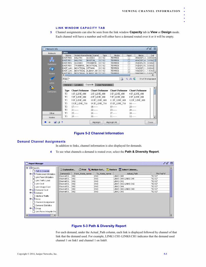
Link Window Capacity Tab 5-3
Demand Channel Assignments 5-3
6 Designing for the Transport Model 6-1Prerequisites 6-1Related Documentation 6-1Overview 6-1
Design > Design 6-1
Design>Diversity Design 6-1
Design>Path Design 6-1
Diverse Path Design 6-2Viewing Diverse Paths 6-2
Designing Diverse Paths 6-4
Design Examples for Diverse Paths for 1+1 and Virtual Concatenation 6-5“Virtual-Concatenation” Diverse (VCATD) Paths and Div Path Design 6-7
7 Failure Simulation 7-1Prerequisites 7-1Related Documentation 7-1Overview 7-1UPSR ring failure 7-2BLSR ring failure 7-2Failure over multiple rings 7-3Mesh Restoration 7-41+1 Path Protection 7-4
8 Multi-Layer Analysis 8-1Overview 8-1Basic Requirements for Multiple-Layer Analysis 8-1Delay analysis for the IP Network links 8-2
Path Report and Failure simulation 8-3
Relating information back to the IP Layer 8-3
Failure simulation across multiple layers 8-4“Updown.runcode” file: 8-4
“SRLG.runcode” file: 8-4
Reading the SRLG file into the IP Network model 8-5Example of Multi-Layer Simulation 8-6
9 Multi-Layer Import 9-1Prerequisites 9-1Overview 9-1Import Wizard 9-2
Appending to a demand file, Using Layer Names, 9-3
Node Name Mapping File Format 9-5
Link Type Mapping File 9-5
Copyright © 2014, Juniper Networks, Inc. Contents-3

Example Conversion 9-5
Contents-4 Copyright © 2014, Juniper Networks, Inc.
. . . . .
. . . . . . . . . . . . . . . . . . . . . . . . . . . . . . . . . . .INTRODUCTION 1
PAT-Transport is specifically targeted at network planners from carriers and service providers who need to perform routing, dimensioning, failure simulation, and design studies on a transport network carrying SDH, SONET or WDM services, whether using rings or mesh
architectures or a combination of these. The users of this module may be transport network planners themselves, or planners for other layers such as IP/MPLS, ATM, or Voice, carried on the transport network. NPAT provides sophisticated routing, simulation, and design capabilities including the following:
• Routing: The Transport module can simulate the routing of traffic and rerouting upon failure. Path information is provided down to the channel level.
• Simulation: The module can be used to analyze in detail the impact of transport layer-failures not only on the transport layer (rerouting, etc.) but also on client layers.
• Design: The Transport module supports the design of site-disjoint, link-disjoint, and facility-disjoint traffic paths. In addition, it can be used for capacity planning purposes, by deciding where links need to be purchased in order to meet the traffic requirements for a mesh network, both under normal scenarios (backbone design) and single failure scenarios (backbone diversity design).
NPAT Transport provides the tools needed to model multiservice provisioning platforms (MSPP). It handles a wide range of physical interfaces such as T1/E1, T3/E3, and OC-x/STM-x. It also supports virtual concatenated channels that can be used to model Ethernet services. In addition NPAT Transport handles a variety of protection options including ring protection, 1+1 path protection, as well as diverse path design for 1+1 paths or for virtual concatenated channels.
Rings and Mesh networksWANDL supports transport networks with rings or mesh network links. Many networks, particularly older networks for well-established operators, are a combination of rings and mesh-network technologies and the routing/failure protection mechanisms work differently in different parts of the network.
For networks with mesh links, demands are protected by broadcasting them over two diverse paths (1+1 path protection); or using the newer technology of path protection mesh-restoration, where the switches in the transport network themselves automatically set up restoration paths for demands affected by a failure; or they may not be protected at all.
For rings, WANDL supports routing on UPSR (SONET) /SNCP (SDH) or BLSR (SONET)/MSP (SDH) rings. For a description of the different ring types modeled in NPAT Transport, refer to Chapter 2, Adding and Modifying Rings.
When rings interconnect at a site, the rings may terminate on a single network element, with each ring usually configured as a shelf on the network element and connection between the rings through the switching fabric in the hardware backplane. Alternatively the add-drop multiplexers (ADMs) that take traffic on and off the individual rings may be physically connected “across the floor”, through the tributary ports on the ADMs.
N
Copyright © 2014, Juniper Networks, Inc. 1-1
I N T R O D U C T I O N
Mult ip le network layers
M U L T I - L A Y E R I M P O R TWANDL supports multi-layer import, which maps the end-to-end demands of one layer to the links in the layer above it. Users can convert links in the source layer (e.g., ATM or IP) to the destination layer (e.g. SONET/SDH). For more details, refer to Chapter 9, Multi-Layer Import of this document or the “Multi-Layer” section of the Network Data Import Wizard chapter of the General Reference Guide.
S H A R E D - R I S K L I N K G R O U P SIn most carriers’ transport networks the transport layer is designed to supply the connectivity for other network layers that directly provide the services to the end-customers. For example an SDH/SONET transport layer will carry the “Packet-over-SONET” (POS) links on the IP network at OC3/STM1, OC12/STM4, OC48/STM16, etc. line rates, either multiplexed into higher bit-rate optical signals over fibres or directly as wavelengths onto DWDM links. Then a failure in the Transport layer will either trigger restoration events which would result in a change in the transmission delay of the affected IP-network links – or cause the failure of a number of POS links in the IP-network. Such multiple-link failures in the IP layer triggered by a single (or otherwise defined) failure event in the Transport network are termed “Shared-Risk-Link Groups” (SRLG). WANDL models SRLG using the facility input file. After creating facilities (logical groups of links and nodes), users can perform failure simulations on facilities and design for facility-disjoint paths.
V I R T U A L C O N C A T E N A T I O NEthernet or Gigabit-Ethernet links may also be carried for long-distances on the transport network by packing into the SDH/SONET frames, “Ethernet-over-SONET” (EOS). There are two standard ways in which this can be done1:
• The Ethernet link can either be carried directly over the next highest SDH/SONET frame size: - e.g. 100Mbps, Fast-Ethernet, carried within a VC4/OC3 (149Mbps) container on the transport layer; or a Gigabit Ethernet carried over a single OC48/STM16 link. This approach can lead to large inefficiencies in the carrying capacity of the network but does not require any further re-combination or buffering in the routers.
• Alternatively, using Virtual-Concatenation (VCAT), the Ethernet link is split into a number of smaller containers that may be routed over different paths in the transport network and then re-combined and re-buffered at the destination router. Using VCAT, a 100-Mbps Fast-Ethernet link would be carried over 3 VC-3 (34Mbps) containers; or a Gigabit-Ethernet link carried over 7 OC3/VC-4 (149Mbps) containers.
If the Ethernet links are carried using VCAT then with Link Capacity Adjustment Scheme (LCAS), a failure in the transport network may result in the loss of only some (not all) of the link’s VCAT containers, since the individual containers may be routed over different paths in the network. This would cause a reduction in the bandwidth or a change in the delay characteristics for the Ethernet link in the IP network, rather than a complete failure of the Ethernet link. Hence, virtual concatenation provides greater bandwidth granularity so that a link can be more efficiently utilized.
NPAT Transport models virtual concatenation groups using n “Virtual concatenated” demands each with the same ID, source node, destination node, and bandwidth. Two flags, VCAT and VCATD, are used to indicate that demands support virtual concatenation/LCAS. These flags can be specified in the demand’s type field.
• Virtual Concatenation Diverse (VCATD): If VCATD is specified, NPAT will try to route the separate demands of the VCG on disjoint paths. Path diversity can be determined as Node/ Link/
1. http://www.cisco.com/en/US/netsol/ns341/ns396/ns114/ns99/networking_solutions_white_paper09186a00801e1215.shtml
1-2 Copyright © 2014, Juniper Networks, Inc.
I N T R O D U C T I O N
. . . . .
Facility/ Shared-Risk-Link-Group diversity in the network as appropriate. Note: The VCATD setting cannot be combined with other protection options.• Virtual Concatenation (VCAT): For VCAT, each of the demands in a Virtual Concatenation Group (VCG) are simply routed independently via the CSPF algorithm. Unlike the VCATD setting, the VCAT setting can be combined with other protection options (default, NOPROT etc.).
Protect ion/Rout ing Opt ions in NPAT-TransportThe routing algorithms in NPAT support a wide range of different protection options for the traffic carried on the network including ring protection mechanisms and mesh protection mechanisms like 1+1 path protection. In addition, one can simulate the effect of removing various protection options such as not configuring protection channels for BLSR/MSP.
• Traffic is protected on UPSR/SNCP/BLSR/MSP rings by the appropriate protection mechanism. For traffic over a single ring, there is an automatic detour upon failure. For traffic across multiple rings, drop and continue mechanisms are the assumed protection mechanism against node failure.
• Paths on a mesh network (or the mesh portion of a mixed network) are automatically restored, modelling the distributed GMPLS control plane of the newer technology, by specifying the RR (reroutable flag)
T R A F F I C P A R A M E T E R SIn summary, the following are the transport-specific traffic parameters:
• Bandwidth: Different sizes from the SONET/SDH multiplexing hierarchy are supported: VC11, VC12, VC3, VC4, VT1.5, VT2, VT3, VT6, STS1, STS3C, STS12C E1, T1, E3, T3, STM1, STM4, STM16, STM64, STM256, OC3, OC12, OC48, OC192, OC768.
• Path Configuration: Users can configure an explicit path down to the card/slot/channel level
• Protection/Reroute Parameters: RR (reroutable), TR (trunk restoration), NORR (nonreroutable), NOPROT (no protection), PR (path required/nonreroutable), PS(path select/preferred), Protected, Unprot (unprotected), UPSR, and Reversion
• Ring Protection Parameters: DRI (dual ring interconnect), PCA (protection channel access/ preemptable)
• Virtual Concatenation (VCAT)/LCAS: VCAT or VCATD (D for diverse paths)
• 1+1: For mesh networks, 1+1 path protection is implemented with a working path and recovery path. NPAT allows for the computation of a node-disjoint, link-disjoint, SRLG(Shared-Risk-Link-Group)-disjoint, and conduit-disjoint protection path. The algorithms incorporate a modification of the Suburelle’s technique to compute strictly diverse paths in situations where the shortest path prevents the calculation of a diverse path.
Design Opt ions
B A C K B O N E L I N K D E S I G N A N D D I V E R S I T Y D E S I G NThe transport module allows backbone link design and diversity design (for redundancy) for mesh networks. Given traffic requirements, design will purchase backbone links as necessary to meet the traffic requirements. Diversity design will purchase backbone links as necessary to meet the traffic requirements under the type of single failure conditions specified by the user. For more details on backbone link design, please refer to the Design & Planning Guide chapter on Design.
D I V E R S E P A T H D E S I G NAdditionally, the program can design paths to be on disjoint paths. The Diverse Path Design feature can then be used for the 1+1 protection feature as well as for designing virtual concatenated channels to be
Copyright © 2014, Juniper Networks, Inc. 1-3
I N T R O D U C T I O N
routed on diverse paths. For more details on path placement design, refer to Chapter 6, Designing for the Transport Model.
Fai lure S imulat ion Opt ionsWith the transport module, users can perform failure simulations to observe the impact of protection mechanisms. After traffic has been rerouted, users can examine the new path placements via path tracing, observe changes in path delay, and view the channels occupied on the new path.
Users can fail various elements including switches, links, and shared risk link groups. These failure simulations can be performed either interactively, through an exhaustive failure simulation script, or using a user-provided up-down sequence. If a simulation script is used such as an exhaustive node or link simulation, the resulting information given will indicate which demands of the transport layer (links of the client layer) failed. This information can be used to create a Shared Risk Link Group for the client layer. In addition, for each failure in the script, NPAT Transport can create an up-down sequence of the corresponding failures in the upper layers for use in a client layer model.
For more information on simulation capabilities and multilayer analysis, refer to Chapter 7, Failure Simulation and Chapter 8, Multi-Layer Analysis.
Channel Report ing FeaturesDetailed channel information can be accessed for links and demands through the link, demand, and path analysis windows or through the following reports:
• Channel assignment report: Indicates the demands routed over each of the channels of a link for mesh and ring links.
• Path & Diversity Report: For a given demand, this report indicates the link channels that the demand is routed over and diversity information such as the virtual concatenation group a demand belongs to, if any.
For more details, refer to Chapter 5, Viewing Channel Information.
Vendor SupportNPAT-Transport supports a number of individual and mixed-vendor solutions and architectures of transport networks – including interconnecting rings or multi-service / multiple ring platforms from vendors such as Alcatel, Cienna, Cisco, ECI, Lucent, Nortel, Marconi; Sycamore or Turin; - or mesh architectures – either based on conventional diverse-path protection or using GMPLS dynamic restoration from vendors such as Alcatel, Marconi and Sycamore.
WANDL can work with the carrier to arrange the data collection to build up the baseline picture of the network architecture and routes – either directly from the network elements or by parsing export reports from the network management system.
1-4 Copyright © 2014, Juniper Networks, Inc.

. . . . .
. . . . . . . . . . . . . . . . . . . . . . . . . . . . . . . . . . .ADDING AND MODIFYING RINGS 2
his chapter provides an overview of the different ring types handled by NPAT Transport and then describes the steps to adding and modifying rings in a network model.
Prerequis i tesPrior to beginning this task, you should have a spec file of the hardware type “Transport.” The network should include the nodes that will belong to the added rings.
Contents1 Ring Types and Parameters in NPAT-Transport on page 2-1.
2 Adding a Ring on page 2-4.
3 Modifying a Ring on page 2-7.
4 Duplicating a Ring on page 2-8.
5 Deleting Rings on page 2-9.
6 Ring File Format on page 2-10 and Link File Format on page 2-10
Ring Types and Parameters in NPAT-TransportThis section describes the following ring types available using NPAT transport and parameters available for them:
• Unidirectional Path Switch Ring (UPSR)
• Sub-Network Connection Protection (SNCP)
• Bi-directional Line Switch Rings (BLSR)
• Multiplex Section-Shared Protection Ring (MSPR)
U P S R ( S O N E T ) / S N C P ( S D H ) R I N G SIn UPSR/SNCP rings, protected traffic is broadcast both ways around the ring. Hence the same demand occupies the same channel(s) everywhere on the ring.
Figure 2-1 UPSR/SNCP Ring Path Protection
T
Copyright © 2014, Juniper Networks, Inc. 2-1
A D D I N G A N D M O D I F Y I N G R I N G S
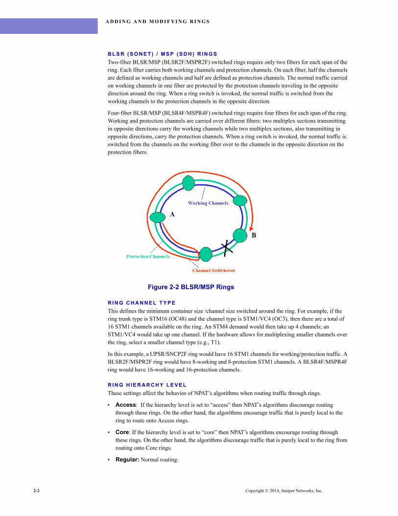
B L S R ( S O N E T ) / M S P ( S D H ) R I N G STwo-fiber BLSR/MSP (BLSR2F/MSPR2F) switched rings require only two fibers for each span of the ring. Each fiber carries both working channels and protection channels. On each fiber, half the channels are defined as working channels and half are defined as protection channels. The normal traffic carried on working channels in one fiber are protected by the protection channels traveling in the opposite direction around the ring. When a ring switch is invoked, the normal traffic is switched from the working channels to the protection channels in the opposite direction.
Four-fiber BLSR/MSP (BLSR4F/MSPR4F) switched rings require four fibers for each span of the ring. Working and protection channels are carried over different fibers: two multiplex sections transmitting in opposite directions carry the working channels while two multiplex sections, also transmitting in opposite directions, carry the protection channels. When a ring switch is invoked, the normal traffic is switched from the channels on the working fiber over to the channels in the opposite direction on the protection fibers.
Figure 2-2 BLSR/MSP Rings
R I N G C H A N N E L T Y P EThis defines the minimum container size /channel size switched around the ring. For example, if the ring trunk type is STM16 (OC48) and the channel type is STM1/VC4 (OC3), then there are a total of 16 STM1 channels available on the ring. An STM4 demand would then take up 4 channels; an STM1/VC4 would take up one channel. If the hardware allows for multiplexing smaller channels over the ring, select a smaller channel type (e.g., T1).
In this example, a UPSR/SNCP2F ring would have 16 STM1 channels for working/protection traffic. A BLSR2F/MSPR2F ring would have 8-working and 8-protection STM1 channels. A BLSR4F/MSPR4F ring would have 16-working and 16-protection channels.
R I N G H I E R A R C H Y L E V E LThese settings affect the behavior of NPAT’s algorithms when routing traffic through rings.
• Access: If the hierarchy level is set to “access” then NPAT’s algorithms discourage routing through these rings. On the other hand, the algorithms encourage traffic that is purely local to the ring to route onto Access rings.
• Core: If the hierarchy level is set to “core” then NPAT’s algorithms encourage routing through these rings. On the other hand, the algorithms discourage traffic that is purely local to the ring from routing onto Core rings.
• Regular: Normal routing.
2-2 Copyright © 2014, Juniper Networks, Inc.
A D D I N G A N D M O D I F Y I N G R I N G S
. . . . .
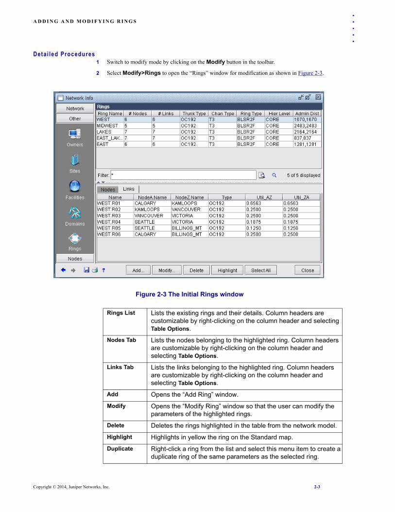
Deta i led Procedures1 Switch to modify mode by clicking on the Modify button in the toolbar.
2 Select Modify>Rings to open the “Rings” window for modification as shown in Figure 2-3.
Figure 2-3 The Initial Rings window
Rings List Lists the existing rings and their details. Column headers are customizable by right-clicking on the column header and selecting Table Options.
Nodes Tab Lists the nodes belonging to the highlighted ring. Column headers are customizable by right-clicking on the column header and selecting Table Options.
Links Tab Lists the links belonging to the highlighted ring. Column headers are customizable by right-clicking on the column header and selecting Table Options.
Add Opens the “Add Ring” window.
Modify Opens the “Modify Ring” window so that the user can modify the parameters of the highlighted rings.
Delete Deletes the rings highlighted in the table from the network model.
Highlight Highlights in yellow the ring on the Standard map.
Duplicate Right-click a ring from the list and select this menu item to create a duplicate ring of the same parameters as the selected ring.
Copyright © 2014, Juniper Networks, Inc. 2-3
A D D I N G A N D M O D I F Y I N G R I N G S
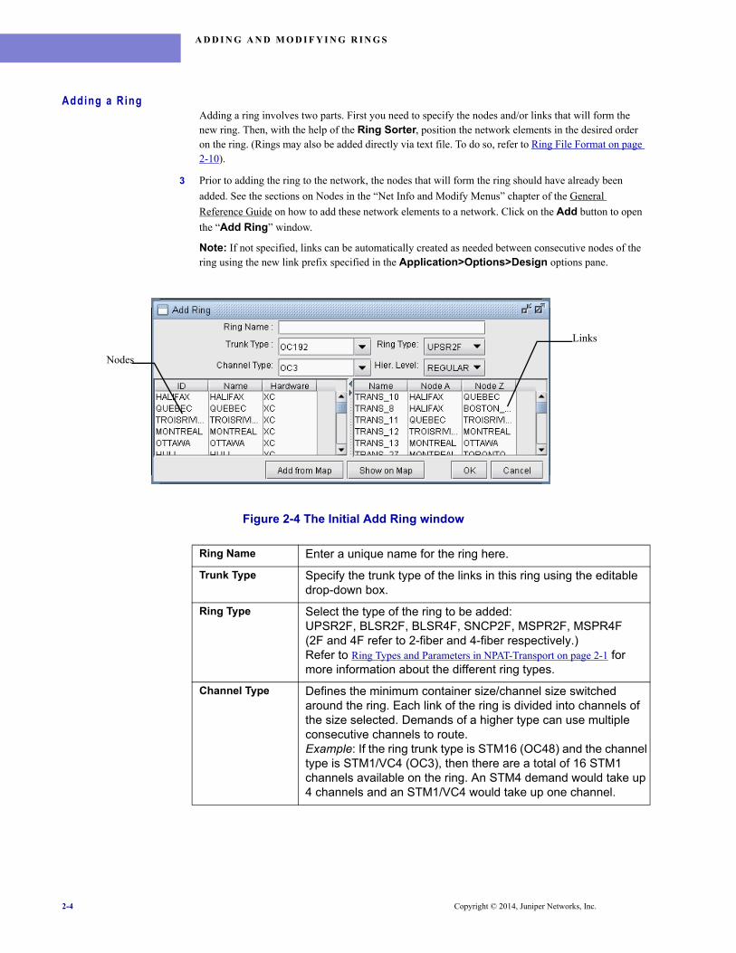
Adding a RingAdding a ring involves two parts. First you need to specify the nodes and/or links that will form the new ring. Then, with the help of the Ring Sorter, position the network elements in the desired order on the ring. (Rings may also be added directly via text file. To do so, refer to Ring File Format on page 2-10).
3 Prior to adding the ring to the network, the nodes that will form the ring should have already been
added. See the sections on Nodes in the “Net Info and Modify Menus” chapter of the General
Reference Guide on how to add these network elements to a network. Click on the Add button to open
the “Add Ring” window.
Note: If not specified, links can be automatically created as needed between consecutive nodes of the ring using the new link prefix specified in the Application>Options>Design options pane.
Figure 2-4 The Initial Add Ring window
Ring Name Enter a unique name for the ring here.
Trunk Type Specify the trunk type of the links in this ring using the editable drop-down box.
Ring Type Select the type of the ring to be added: UPSR2F, BLSR2F, BLSR4F, SNCP2F, MSPR2F, MSPR4F(2F and 4F refer to 2-fiber and 4-fiber respectively.)Refer to Ring Types and Parameters in NPAT-Transport on page 2-1 for more information about the different ring types.
Channel Type Defines the minimum container size/channel size switched around the ring. Each link of the ring is divided into channels of the size selected. Demands of a higher type can use multiple consecutive channels to route. Example: If the ring trunk type is STM16 (OC48) and the channel type is STM1/VC4 (OC3), then there are a total of 16 STM1 channels available on the ring. An STM4 demand would take up 4 channels and an STM1/VC4 would take up one channel.
Links
Nodes
2-4 Copyright © 2014, Juniper Networks, Inc.
A D D I N G A N D M O D I F Y I N G R I N G S
. . . . .
4 First, enter a name for the ring in the “Ring Name” text box, e.g., “MyRing.” Next, specify the ring’s
trunk hardware type and channel type in the “Trunk Type” and “Channel Type” fields by typing in a
name in the text area or clicking on the down arrow to select from the list. Specify the type of ring you
want and the ring’s hierarchy level by clicking on the drop-down list and selecting one from the list.
5 The bottom half of the Add Ring window lists the existing nodes and the available links matching the
selected trunk type. Select the nodes and links that will be used to form the ring. If you would like the
program to automatically add new links for you, leave the Links list empty.
You can select the nodes and links from the map and then press the Add from Map button to make the selection of nodes and rings for the ring. Alternatively, nodes/links can also be selected directly from the list by clicking or dragging the mouse across the desired rows and/or by using <Ctrl>-click or <Shift>-click to select multiple rows. Double-click on the column header to sort the table by that column.
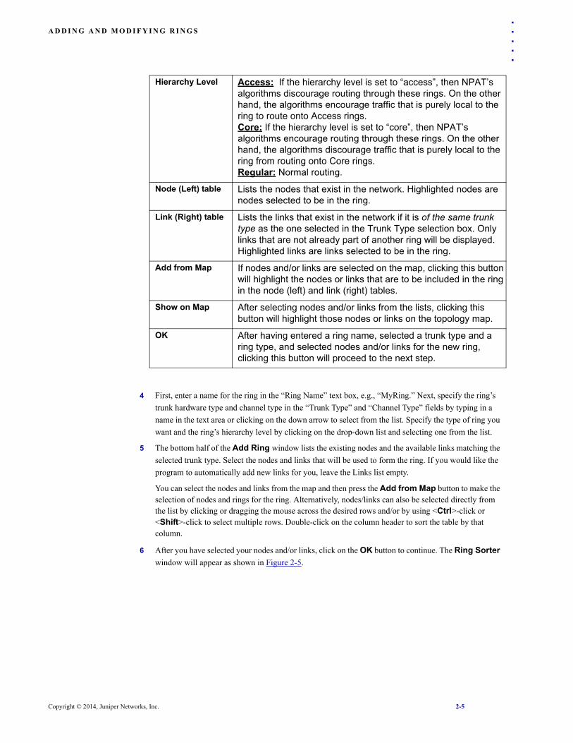
6 After you have selected your nodes and/or links, click on the OK button to continue. The Ring Sorter
window will appear as shown in Figure 2-5.
Hierarchy Level Access: If the hierarchy level is set to “access”, then NPAT’s algorithms discourage routing through these rings. On the other hand, the algorithms encourage traffic that is purely local to the ring to route onto Access rings. Core: If the hierarchy level is set to “core”, then NPAT’s algorithms encourage routing through these rings. On the other hand, the algorithms discourage traffic that is purely local to the ring from routing onto Core rings. Regular: Normal routing.
Node (Left) table Lists the nodes that exist in the network. Highlighted nodes are nodes selected to be in the ring.
Link (Right) table Lists the links that exist in the network if it is of the same trunk type as the one selected in the Trunk Type selection box. Only links that are not already part of another ring will be displayed. Highlighted links are links selected to be in the ring.
Add from Map If nodes and/or links are selected on the map, clicking this button will highlight the nodes or links that are to be included in the ring in the node (left) and link (right) tables.
Show on Map After selecting nodes and/or links from the lists, clicking this button will highlight those nodes or links on the topology map.
OK After having entered a ring name, selected a trunk type and a ring type, and selected nodes and/or links for the new ring, clicking this button will proceed to the next step.
Copyright © 2014, Juniper Networks, Inc. 2-5
A D D I N G A N D M O D I F Y I N G R I N G S
Figure 2-5 Ring Sorter window
7 Using the ordering tools in this window (e.g. wheel, shortest), arrange the nodes in the order that you
want. If links were selected for the ring, rearrange the nodes as necessary by dragging them to other
points along the circle to eliminate any link crossing. Click Show to see how the ring would look on
the topology map.
8 Click OK to add the ring. The new ring will be added to the rings list in the “Rings” window showing
its corresponding nodes on the bottom. Select the newly added ring to view the nodes and links of the
ring.
9 The Add Ring window remains open in case you would like to add another ring. If you are finished
adding rings, select the Cancel button of the Add Ring window to close it.
Wheel Sorts the nodes into a wheel around the geographic center.
Shortest This button re-arranges the nodes in the circle to the shortest distances between the nodes.
Reset Resets the order of the nodes around the ring to the original order.
Show Highlights the ring with its nodes and corresponding links on the topology map in the order that is shown in this window. The purple-colored links represent links that already exist in the network. The orange-colored links represent links that do not already exist and need to be purchased and added to the network.
OK Ring links will be added in the order of the nodes in the circle.
2-6 Copyright © 2014, Juniper Networks, Inc.
A D D I N G A N D M O D I F Y I N G R I N G S
. . . . .
Modi fy ing a Ring10 Select Modify>Rings to open the rings window. Alternatively, you may modify a ring by right-
clicking on the node on which the ring exists and selecting Modify Rings On Node. Similarly, you
may modify a ring by right-clicking on a link on which the ring exists and clicking Modify Rings On Link.
11 Select an entry from the list that you want to modify and click the Modify button. The Modify Ring window will appear as shown in Figure 2-6.
Figure 2-6 Modify Ring window
12 Change the fields that you want to modify and click OK to proceed to the next step.
13 Move the nodes around in the “Ring Sorter” window if necessary. When done, click OK.
14 If nodes were added, removed, or if nodes were moved around, some links may not be needed anymore
and the program will ask you if you want to delete the links that are not between consecutive nodes.
They will be removed from the ring, but you can choose whether or not to delete them from the
network entirely. Selecting Yes will remove the links from the ring and the network. Selecting No will
only remove the links from the ring, but keep them in the network.
Figure 2-7 Option to Delete Unused Links
15 You may also modify multiple rings at the same time. In the Ring modification window, select one or
more rows to modify, and then click the Modify button. Change the fields that you want to modify and
click OK.
Copyright © 2014, Juniper Networks, Inc. 2-7
A D D I N G A N D M O D I F Y I N G R I N G S
Figure 2-8 Modifying Multiple Rings
Dupl icat ing a RingThis function will create duplicates of an existing ring, utilizing the same ring type, trunk type, and nodes. However, new links would need to be purchased for the new ring. In the routing aspect, identical or duplicate rings are treated as one stack of rings. The channels in rings that are on the same stack are filled in sequential order. If the oversubscription flag is turned on, oversubscription will only occur at the last ring of each stack. Backup channels are used during failure simulation.
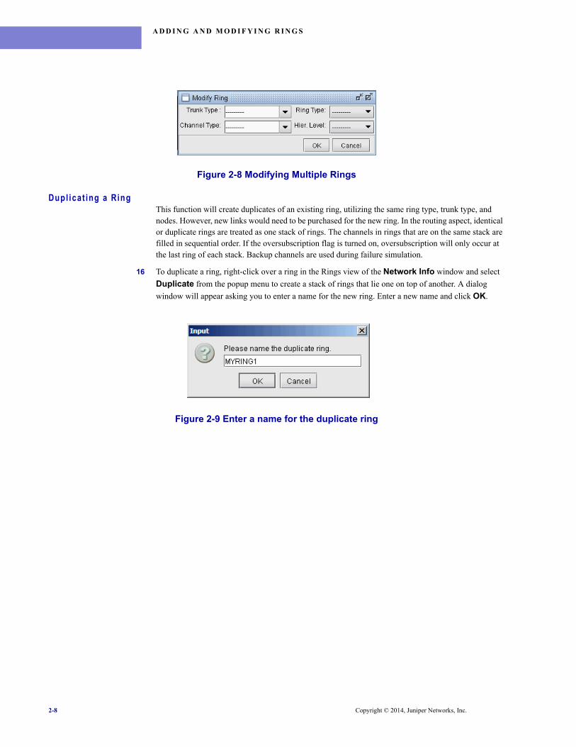
16 To duplicate a ring, right-click over a ring in the Rings view of the Network Info window and select
Duplicate from the popup menu to create a stack of rings that lie one on top of another. A dialog
window will appear asking you to enter a name for the new ring. Enter a new name and click OK.
Figure 2-9 Enter a name for the duplicate ring
2-8 Copyright © 2014, Juniper Networks, Inc.
A D D I N G A N D M O D I F Y I N G R I N G S
. . . . .
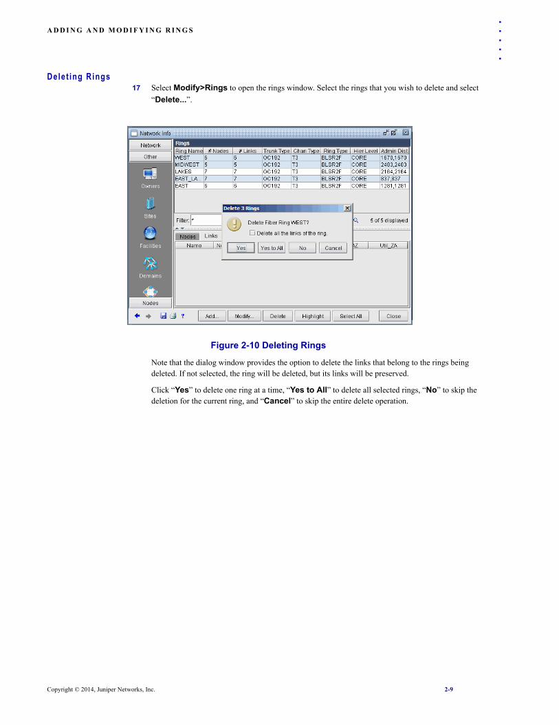
Delet ing Rings17 Select Modify>Rings to open the rings window. Select the rings that you wish to delete and select
“Delete...”.
Figure 2-10 Deleting Rings
Note that the dialog window provides the option to delete the links that belong to the rings being deleted. If not selected, the ring will be deleted, but its links will be preserved.
Click “Yes” to delete one ring at a time, “Yes to All” to delete all selected rings, “No” to skip the deletion for the current ring, and “Cancel” to skip the entire delete operation.
Copyright © 2014, Juniper Networks, Inc. 2-9
A D D I N G A N D M O D I F Y I N G R I N G S
Ring F i le FormatUpon saving a network with transport rings, a ring file will be created, with a line for each ring containing the ring characteristics followed by an ordered comma separated list of nodes and links in the ring. This file should be referenced in the spec file using the entry “ring=ringfilename” where ringfilename is substituted by the name or path of the ring file.
F I L E F O R M A TRingName TrunkType RingType ChannelType HierarchyLevel Ordered_List_of_Nodes_and_links
E X A M P L E SRING1 OC48 BLSR4F T3 - N1, LINK1,N2, LINK2,N3, LINK3,N4, LINK4,N5, LINK5,RING2 OC48 BLSR2F T3 CORE A, LINK_AB, B, LINK_BC, C, LINK_CA
Link F i le FormatThe following is an example of the link file format for both ring and mesh links. This file can be referenced in the spec file using the entry “bblink=linkfilename” where linkfilename is substituted by the name or path of the link file.
#LinkName Node Node Vendor # BwType [Misc]LINK1 N1.C1P1 N2.C3P1 DEF 1 OC48
Note that the card and slot occupied by the link can be indicated for the link endpoints. In the example above, LINK1 connects slot 1 port 1 of node N1 to slot 3 port 1 of node N2.
For mesh links, to indicate a minimum size for the channel type, specify CHAN=bwtype in the Misc field. Example: using CHAN=T3 for the miscellaneous field would prevent channels smaller than an STS1 from being directly routed over this link.
Field Description
RingName A user-specified name for the ring
TrunkType The type of link used for this ring (e.g., OC48, OC192)
RingType The ring category and number of fibers. For example, BLSR2F stands for Bidirectional Line Switched Ring (Options include BLSR2F, BLSR4F, UPSR2F, SNCP2F, MSPR2F, MSPR4F.)
ChannelType The size of the channel that this ring is divided into. For example, if the channel type is T3 (the equivalent of an OC1), an OC3 demand will occupy three such channels.
HierarchyLevel CORE, ACCESS, or REGULAR. A dash (‘-’) also represents regular. Refer to Adding a Ring on page 2-4 for a further description of this field.
Ordered_List_of_Nodes_and_Links
A comma separated list of ordered nodes and links that make up the ring. This list can start with any node of the ring. Note: The space between link,node pairs is not required.
2-10 Copyright © 2014, Juniper Networks, Inc.

. . . . .
. . . . . . . . . . . . . . . . . . . . . . . . . . . . . . . . . . .VIEWING RING INFORMATION 3
his chapter provides an overview of viewing ring information through the application.
Prerequis i tesPrior to beginning this task, you should have a spec file of the hardware type “Transport.” To follow along, use the sample/transport/ring/spec.ring network in the WANDL_HOME, or /u/wandl/, directory.
Contents1 Accessing the Ring Window on page 3-1
2 View Node/Link Info for a Ring on page 3-2
3 Highlight Rings on page 3-2
4 Filter Rings on page 3-2
5 Filtering Rings for the Map on page 3-3
6 Viewing/Customizing the Ring Map on page 3-3
Deta i led Procedures
Accessing the Ring Window1 In View or Design mode, select Net Info>Ring>View Rings.
Figure 3-1 View Rings window
Note the last column Admin Dist. provides a sum of the admin weights of the links in the ring.
T
Copyright © 2014, Juniper Networks, Inc. 3-1
VI E W I N G R I N G I N F O R M A T I O N
View Node/L ink In fo for a Ring2 Select a ring from the upper half of the window to display its node and link information in the bottom
half. To obtain more detailed information on the nodes and links of the ring, click the Node Details
and Link Details buttons to open up the Node window or Link window filtered to include only the
nodes or links in the ring.
Highl ight R ings3 To highlight one or more rings on the map, select one or more rings from the table, by clicking the first
ring to highlight and then <Ctrl>-clicking additional rows to add them or <Shift>-clicking to add a
range of rows starting from the last selected row. Then click the Highlight... button.
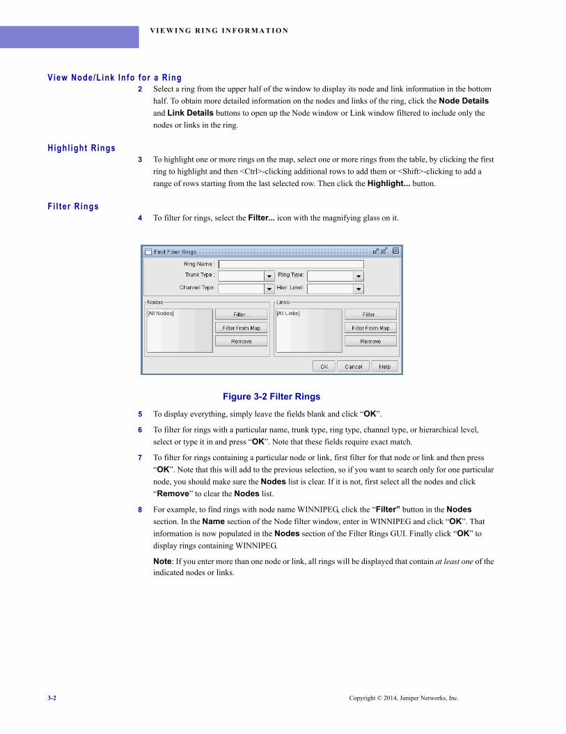
Fi l ter R ings4 To filter for rings, select the Filter... icon with the magnifying glass on it.
Figure 3-2 Filter Rings
5 To display everything, simply leave the fields blank and click “OK”.
6 To filter for rings with a particular name, trunk type, ring type, channel type, or hierarchical level,
select or type it in and press “OK”. Note that these fields require exact match.
7 To filter for rings containing a particular node or link, first filter for that node or link and then press
“OK”. Note that this will add to the previous selection, so if you want to search only for one particular
node, you should make sure the Nodes list is clear. If it is not, first select all the nodes and click
“Remove” to clear the Nodes list.
8 For example, to find rings with node name WINNIPEG, click the “Filter” button in the Nodes
section. In the Name section of the Node filter window, enter in WINNIPEG and click “OK”. That
information is now populated in the Nodes section of the Filter Rings GUI. Finally click “OK” to
display rings containing WINNIPEG.
Note: If you enter more than one node or link, all rings will be displayed that contain at least one of the indicated nodes or links.
3-2 Copyright © 2014, Juniper Networks, Inc.
VI E W I N G R I N G I N F O R M A T I O N
. . . . .
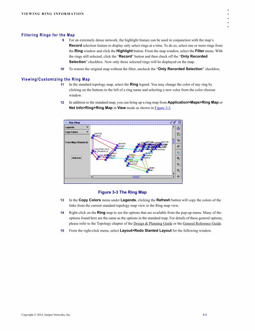
Fi l ter ing Rings for the Map9 For an extremely dense network, the highlight feature can be used in conjunction with the map’s
Record selection feature to display only select rings at a time. To do so, select one or more rings from
the Ring window and click the Highlight button. From the map window, select the Filter menu. With
the rings still selected, click the “Record” button and then check off the “Only Recorded Selection” checkbox. Now only those selected rings will be displayed on the map.
10 To restore the original map without the filter, uncheck the “Only Recorded Selection” checkbox.
Viewing/Customiz ing the Ring Map11 In the standard topology map, select the Ring legend. You may change the color of any ring by
clicking on the buttons to the left of a ring name and selecting a new color from the color chooser
window.
12 In addition to the standard map, you can bring up a ring map from Application>Maps>Ring Map or
Net Info>Ring>Ring Map in View mode as shown in Figure 3-3.
Figure 3-3 The Ring Map
13 In the Copy Colors menu under Legends, clicking the Refresh button will copy the colors of the
links from the current standard topology map view to the Ring map view.
14 Right-click on the Ring map to see the options that are available from the pop-up menu. Many of the
options found here are the same as the options in the standard map. For details of these general options,
please refer to the Topology chapter of the Design & Planning Guide or the General Reference Guide.
15 From the right-click menu, select Layout>Redo Slanted Layout for the following window.
Copyright © 2014, Juniper Networks, Inc. 3-3

VI E W I N G R I N G I N F O R M A T I O N
Figure 3-4 Choose Offset window
Note: If node A is on multiple or overlapping rings (say “n” different rings), it is exploded on the Ring Map into n separate nodes: A_R0, A_R1, ..., A_Rn. This way, it will be easier to differentiate between different rings, where each piece is a polygon in the rough shape of a circle. The A_R's are initially laid out near where A was on the main map, and are spread out along a line slanting northeast.
16 In this window, the user may specify using (x,y) coordinate settings how exploded nodes can be shown
on the Ring map. The default setting is (6,12), in which case the first, second, and third layers are
slanted to the top and to the right in the example above.
17 Change the coordinates to (0,30) and you will notice that the three layers will be aligned vertically in a
straight line and the layers will be further apart. Click OK to see the effects of this layout on the Ring
map. See the change in Figure 3-5.
Figure 3-5 Ring map with adjusted slant layout
3-4 Copyright © 2014, Juniper Networks, Inc.
. . . . .
. . . . . . . . . . . . . . . . . . . . . . . . . . . . . . . . . . .LINK AND TRAFFIC PARAMETERS 4
his chapter describes the steps for adding and modifying links and traffic for both mesh and ring networks. In this chapter, you will learn how to specify demand routing and protection options and how to configure virtual trunks, demands that themselves can carry demands. For
links, you will learn how to specify information about lambdas and specify trunktype and card/port information.
Prerequis i tesPrior to beginning this task, you must have created a spec file or opened a spec file as described in the Design & Planning Guide. More specifically, the network model must be of the hardware type “Transport” in order for these features to be available.
Related Documentat ionFor general traffic parameter modification instructions, refer to the Design & Planning Guide and File Format Guide.
Overv iew1 Specifying the Bandwidth on page 4-1
2 Specifying a Configured Path on page 4-2
3 Specifying Protection/Routing Options on page 4-2
4 Configuring Virtual Trunk Map Settings on page 4-5
5 Specifying 1+1 Path Protection on page 4-6
6 Specifying Virtual Concatenation and Link Capacity Adjustment Scheme on page 4-7
7 Modeling Conduits (Sycamore) on page 4-8
8 Modeling Reversion (Sycamore) on page 4-9
9 Example Mappings on page 4-10
10 Link Configuration on page 4-14
11 WDM Specification on page 4-14
Speci fy ing the Bandwidth1 To add traffic through the graphical interface, switch to modify mode by clicking on the Modify button
in the toolbar. Then select Modify>Demands>Add/Modify/Delete... and then click the Add button
and select One Demand... to add a single demand. (To add traffic via text file, see Example
Mappings on page 4-10.)
2 Under BW (Bandwidth), select the bandwidth type: e.g., VC11, VC12, VC3, VC4, VT1.5, VT2, VT3,
VT6,STS1,STS3C,STS12C,E1,T1,E3,T3,STM1,STM4,STM16,STM64,STM256,OC3,OC12,OC48,
OC192,OC768.
T
Copyright © 2014, Juniper Networks, Inc. 4-1
L I N K A N D TR A F F I C P A R A M E T E R S
Speci fy ing a Conf igured Path3 The path is indicated under Configured Route in the table in the bottom half of the window and
consists of an ordered list of nodes and links separated by dashes. To add a path specification from the
map, select the nodes/links of the path from the map, right-click in the table, and select “Use Map Sel’n”.
4 To edit the path manually, double-click the cell in the table under Configured Route.
5 Information about the occupied card/slot/channel can be indicated for the nodes along the path by
adding a suffix to the node as follows:
S T S C H A N N E L N A M I N G C O N V E N T I O NCHn_m (the mth channel in the nth STS-1)CHSTSn_m_k (the kth T1 in the mth T2 in the nth STS-1)
Example:N4.C5P4CH10 for NodeID N4, slot 5, port 4, 10th channelN6.C5P4CHSTS1_3_2 for NodeID N6, slot 5, port 4, 1st STS1's 2nd T1 channel in the 3rd T2.
6 In addition to the conventional path specification using “dashes” to separate the nodes and links of the
path, ring and channel information can also be included in the path specification as follows:
I N C L U D I N G R I N G S I N T H E P A T HnodeA-ringname-nodeZ
or nodeA-ringname.CHn-nodeZor nodeA-ringname.CHn_m_x-nodeZ
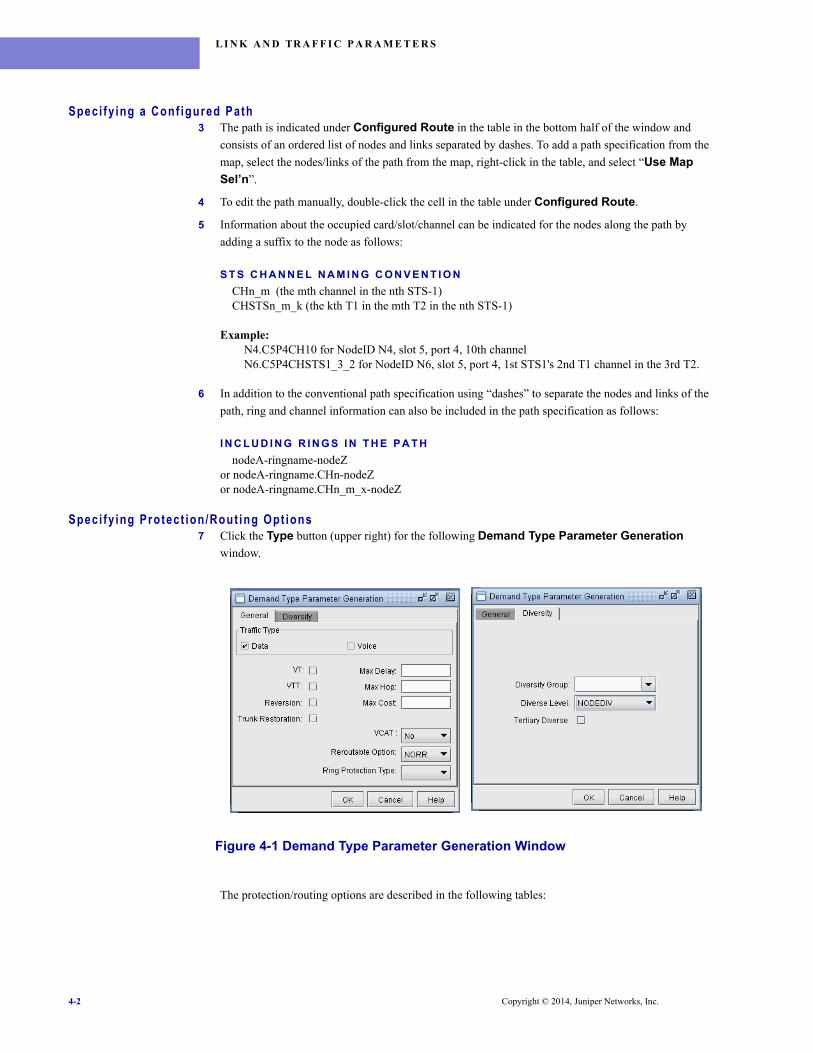
Speci fy ing Protect ion/Rout ing Opt ions7 Click the Type button (upper right) for the following Demand Type Parameter Generation
window.
Figure 4-1 Demand Type Parameter Generation Window
The protection/routing options are described in the following tables:
4-2 Copyright © 2014, Juniper Networks, Inc.
L I N K A N D TR A F F I C P A R A M E T E R S
. . . . .
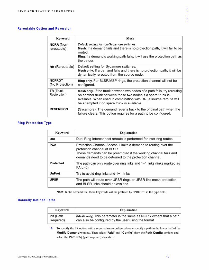
Reroutable Opt ion and Revers ionRing Protect ion Type
Note: In the demand file, these keywords will be prefixed by “PROT=” in the type field.
Manual ly Def ined Paths
8 To specify the PR option with a required user-configured route specify a path in the lower half of the
Modify Demand window. Then select “Add” and “Config” from the Path Config. options and
select the Path Req (path required) checkbox.
Keyword Mesh
NORR (Non-reroutable)
Default setting for non-Sycamore switches.Mesh: If a demand fails and there is no protection path, it will fail to be routed. Ring:If a demand’s working path fails, it will use the protection path as the detour.
RR (Reroutable) Default setting for Sycamore switches.Mesh only. If a demand fails and there is no protection path, it will be dynamically rerouted from the source node.
NOPROT(No Protection)
Ring only. For BLSR/MSP rings, the protection channel will not be configured.
TR (Trunk Restoration)
Mesh only. If the trunk between two nodes of a path fails, try rerouting on another trunk between those two nodes if a spare trunk is available. When used in combination with RR, a source reroute will be attempted if no spare trunk is available.
REVERSION (Sycamore). The demand reverts back to the original path when the failure clears. This option requires for a path to be configured.
Keyword Explanation
DRI Dual Ring Interconnect reroute is performed for inter-ring routes.
PCA Protection-Channel Access. Limits a demand to routing over the protection channel of BLSR.These demands can be preempted if the working channel fails and demands need to be detoured to the protection channel.
Protected The path can only route over ring links and 1+1 links (links marked as FAIL=0).
UnProt Try to avoid ring links and 1+1 links
UPSR The path will route over UPSR rings or UPSR-like mesh protection and BLSR links should be avoided.
Keyword Explanation
PR (Path Required)
(Mesh only) This parameter is the same as NORR except that a path can also be configured by the user using the format
Copyright © 2014, Juniper Networks, Inc. 4-3
L I N K A N D TR A F F I C P A R A M E T E R S
Divers i ty Opt ions
Vir tua l Concatenat ion Opt ions
Vir tua l Trunk
Keyword Explanation
1+1 The demand is routed across a primary and protection path. If the primary path fails, the protection path will be used. (Note that if the switches are specified as Sycamore switches, only one path will be routed if the diversity constraints cannot be satisfied.)1+1 is not configured through the Demand Type Generation window. See Specifying 1+1 Path Protection on page 4-6 for instructions on how to configure 1+1 through the Path Config. Options.
CONDUITDIV (For use in combination with 1+1). The demand will be routed across two conduit-diverse paths if possible. See Specifying Conduits for Conduit Diverse Routing on page 4-14 to define the conduit(s) associated with a link.
NODEDIV (For use in combination with 1+1). The demand will be routed across two paths which are both node-disjoint and conduit-disjoint if possible.
Option Description
VCAT Virtual concatenation. This option groups demands together as part of a virtual concatenation group (VCG). When a design is run the demands will try to route along the same path as each other. See Specifying Virtual Concatenation and Link Capacity Adjustment Scheme on page 4-7 for creating a VCG.
VCATD Virtual concatenation diverse. This option is similar to VCAT except that when a design is run, the demands will be routed diversely from each other. NPAT groups the entries marked with VCATD in pairs. The two demands in the same pair are routed diversely whenever possible. Furthermore, the VCATD setting cannot be combined with other protection options, whereas VCAT can.
Keyword Explanation
VT Stands for Virtual Trunk. Check off the “VT” option to indicate the demand is itself a container that can have other demands routed over it. Upon updating the network state, a link will be created for each VT. These links can be used as mesh links or they can be used to form a ring through the ring window’s add option.
See Configuring Virtual Trunk Map Settings on page 4-5 for viewing options.
VTT VTT stands for VT Tunnel and is used for Cisco ONS model for a T3 channel which can carry 28 VT1.5. Unlike a VT, the demands carried by the VTT should have the same source and destination as the VTT. Upon updating the network state, a link will be created for each VT whose map settings can be customized similar to the VT.
4-4 Copyright © 2014, Juniper Networks, Inc.
L I N K A N D TR A F F I C P A R A M E T E R S
. . . . .
Conf igur ing Vi r tua l Trunk Map Set t ings9 As mentioned earlier, a virtual trunk is a virtual container routed over a link that itself can have
demands routed over it. It is specified in the WANDL file format as a demand and occupies the
bandwidth of the link it is routed over. When the spec file is open, the program will automatically
create a corresponding link to represent the virtual trunk. Demands that should be routed over the
virtual trunk should indicate the virtual trunk in the path configuration.
10 After adding a virtual trunk, the virtual trunk display options can be set from
Application>Options>Map Preferences. VT links are colored purple by default. To change the
color, double-click the color box to the right of “Virtual Trunks” to change the color. To override this
setting and instead color according to the legends (Prov Util, etc.), select the checkbox for “Show VT as normal”. To hide VTs from the map altogether, select the Filters menu from the upper menu of
the map’s left pane. Then select the checkbox “Hide VT”
Figure 4-2 Virtual Trunk Settings in the Map Preferences options pane
11 When double-clicking a link that corresponds to a virtual trunk, the link window will display a “View VT Path...” button to display the path taken by the virtual trunk as a demand over the transport layer.
Copyright © 2014, Juniper Networks, Inc. 4-5
L I N K A N D TR A F F I C P A R A M E T E R S
Speci fy ing 1+1 Path Protect ionNPAT can perform the following for 1+1 path protection for meshed and ring networks if 1+1 is selected for the path config option.
• For the meshed network, a disjoint path will be created by the program for the demand and capacity will be reserved for the path.
• For the ring network, whether UPSR/SNCP or BLSR/MSP, the detour path is implied. For demand paths across multiple rings, the demand is assumed to be protected against node failure, with the Drop & Continue mechanism to protect across the rings.
Note: The demand with 1+1 path protection will be considered to be up if either the main path or the protection path are up.
A D D I N G D E M A N D S12 In the add demand window, specify 1+1 protection by selecting 1+1 under Path Config. Options.
Figure 4-3 Add Demand Window: Selecting 1+1 Protection
M O D I F Y I N G D E M A N D S13 To add or remove 1+1 protection for existing demands, select Modify>Demands>
Add/Modify/Delete... Then select the demands to be modified and click Modify... Under Path Config. Options, select either Add or Remove from the first selection box. In the following
selection box, select 1+1.
Figure 4-4 Modify Demand Window: Adding 1+1 protection to an existing demand
Once 1+1 protection is specified, a protection path will automatically be created. To design the paths to be on disjoint paths, refer to Diverse Path Design on page 6-2 for further details.
4-6 Copyright © 2014, Juniper Networks, Inc.
L I N K A N D TR A F F I C P A R A M E T E R S
. . . . .
Speci fy ing V i r tua l Concatenat ion and L ink Capaci ty Adjustment Scheme14 To indicate virtual concatenation, the virtual containers of the virtual concatenation group (VCG)
should be entered in as demands with the same demand ID and from and to nodes. To add these
demands, select Modify>Demands>Add Multiple Demands. The example below indicates the
VCG for an Ethernet signal, modeled using seven VC-11’s (VC-11-7v).
Figure 4-5 Adding a Virtual Concatenation Group
Note that this is equivalent to adding the following line to a demand input file and then importing the demand file via the File>Read menu:
Ethernet10M_VCG1 N2 N0 VC11 R7,VCAT 2,2
15 Click the Type button (upper right) for the Demand Type Parameter Generation window.
For the VCAT (Virtual Concatenation) parameter, you can select VCAT or VCATD depending on whether you would like demands to be routed on disjoint paths or not if possible.
Note: NPAT Transport does not support combining both the VCAT and 1+1 flag together.
Copyright © 2014, Juniper Networks, Inc. 4-7
L I N K A N D TR A F F I C P A R A M E T E R S
Model ing Condui ts (Sycamore)Conduits can be marked on links in order to influence demands with conduit-diverse routes. The following section explains modifying conduit information through the graphical interface. To edit the bblink file directly, refer to Link Configuration on page 4-14.
U S I N G T H E L I N K M I S C F I E L D T O M O D I F Y C O N D U I T I N F O R M A T I O N16 To indicate that a link belongs to a particular conduit through the graphical interface, first click the
Modify mode button to enter Modify mode. Select Modify>Links... Then select the link(s) to
modify and click the Modify... button. Alternatively, to modify only one link from the map, double-
click on that link.
17 In the Link Modification window, select the Properties tab. In the Misc field, enter in
“CONDUIT=<conduit_list>” where <conduit_list> is replaced by a colon separated list of conduit
names for conduits that the link belongs to. For example, the following Misc field indicates that a link
belongs to conduits c1, c2, and c3.
CONDUIT=c1:c2:c3
18 After modifying the desired links, click the Update button or switch to Design mode.
19 To easily identify from the map which conduits have been defined on a link, right-click over the map
and select Labels>Link Labels>Link Labels... Then select Customize to bring up the Set Labels window. Select the key Misc and then click the “Add” button to display the Misc field on the
link. Select the “Name” key from the right hand side and click the “Remove” button to turn off the
link name label. Then click OK.
20 To delete a conduit for a particular link, double-click the link on the map and erase the Misc field. Note
that this only works for a single link at a time.
U S I N G T H E F A C I L I T Y W I N D O W T O M O D I F Y C O N D U I T I N F O R M A T I O N21 Another method of viewing and modifying the conduit information is through the Facility window. In
Modify mode, select Modify>Facilities. Note that the links are grouped into facilities according to
the shared conduit. Facilities that are Sycamore conduits will be marked with a checkmark under the
Conduit column. Select a conduit and click the Links tab to view the links belonging to the selected
facility. (Note that facilities specially marked as conduits will be saved in the bblink file. The saved
facility file will only list conduits commented out for informational purposes.)
22 To modify the links belonging to a conduit from multiple links, select Modify>Facilities. Then
double-click the facility to be modified. In the resulting window, <Ctrl>-click a selected link entry to
remove the conduit for that link or <Ctrl>-click an unselected link entry to add the conduit for that link.
Click OK when the modification is done. To completely delete a conduit from the network, you can
also select a facility and click the Delete button.
23 After modifying the desired facilities, click the Update button or switch to Design mode. The
miscellaneous field of the associated links will be updated to reflect changes to the conduit.
4-8 Copyright © 2014, Juniper Networks, Inc.
L I N K A N D TR A F F I C P A R A M E T E R S
. . . . .
Model ing Reversion (Sycamore)24 The two applications for reversion are 1.Basic protection with Source Reroute with a manually defined
route and 2. Diverse (1+1) Protection with manually defined routes for the working and protection
routes and without source reroute.
25 To model the former, when adding a demand, select RR and Reversion for the Type field and enter in a
manually defined path in the lower section of the Add or Modify Demand window.
26 To model the latter, when adding a demand, select NORR and Reversion for the Type field select
“Add” “1+1” from the Path Config Options. Then update the network state by clicking the Update
button or Modify>Update Network State. Select Modify>Demands to view the newly created
demand. An additional demand entry with the same name will be listed marked as STANDBY. Double-
click this entry to manually define the route of the protection path in the lower section of the modify
window.
I N T E R A C T I V E S I M U L A T I O N27 To simulate reversion in interactive simulation mode, click the Simulation mode button to enter
Simulation mode. Right-click a link that the demand routed over and select Fail Links under Pointer. Click the Run button to view how the demand routes in the failure simulation.
28 In the Fail Links window, uncheck the link that was failed to bring it back up. Click the Run button to
view how the demand gets rerouted. In this case, it will be rerouted on the original path configured.
U P - D O W N S E Q U E N C E29 To test particular sequences of link up and down events, create an up-down sequence file on the server.
Then select Simulation>Scripts and check Replay Up-Down Sequence file and browse for the
sequence file. Underneath that option, select the option to simulate “Every Event”. Additionally,
select “Reroute Information” under Report Options. Then click the Run button to start the
simulation.
For details on the sequence file format, refer to the File Format Guide, chapter on “Output Files,” section on DAILYSEQ.x Report. The following is an example UPDOWN sequence that will take down two links and then bring them back up:
LINK10 downLINK18 downLINK10 upLINK18 upRESET
30 As a result of the updown sequence simulation, the REPFAIL report will be generated, which will
provide detailed information including the paths before and after demand reroutes. Additionally,
statistics will be provided such as the maximum and average number of hops. With reversion, the hop
count for a particular demand will return to normal when all the links for the configured path are
brought back up. Without reversion, the hop count may increase after a failure and will remain
unchanged until there is another failure on the rerouted path.
Copyright © 2014, Juniper Networks, Inc. 4-9
L I N K A N D TR A F F I C P A R A M E T E R S
Example Mappings
S Y C A M O R E S W I T C H E SSycamore switches (SN16000, SN3000) allow for options for setting the Protection, Source Reroute, Trunk Restoration, and Reversion settings for mesh networks. These map to the following WANDL demand types.
*To manually define a route, substitute configured_path with a complete specification of nodes and/or links from the source to the destination separated by dashes (‘-’). E.g., N1-LINK1-LINK2-N2 indicates a path from Node N1 to Node N2 via the links LINK1 and LINK2.
**See Specifying Conduits for Conduit Diverse Routing on page 4-14 to define conduit(s) associated with a link. For demands originating from Sycamore switches, LINKDIV will be interpreted as the equivalent of CONDUITDIV.
*** Trunk Restoration requires dynamic source reroute (RR) and basic protection.
**** Reversion requires manually configured routing and is incompatible with trunk restoration. Reversion can be simulated either in an interactive simulation or through an up-down sequence simulation script.
Sycamore Feature Options
Corresponding WANDL Demand Type Field
Source Reroute
OnOn with manually defined route*Off Off with manually defined route*
RRRR,PS(configured_path)NORRPR(configured_path)
Protection CONDUIT_ID_DIVERSE**DIVERSELY_ROUTED**BASIC
1+1,CONDUITDIV1+1,NODEDIV(1+1 is not specified)
Trunk Restoration
On***Off
TR(TR is not specified)
Reversion On****Off
REVERSION(REVERSION is not specified)
4-10 Copyright © 2014, Juniper Networks, Inc.
L I N K A N D TR A F F I C P A R A M E T E R S
. . . . .
SION
The following are the valid combinations of the above protection/restoration fields for Sycamore switches and the corresponding WANDL demand types.
Protection/Restoration
Levels ProtectionSource Reroute
Trunk Restorati
on Corresponding WANDL Demand Type
Unrestored Basic Off Off NORRPR(configured_path)
Mesh Restored Basic On Off RRRR,PS(configured_path)RR,PS(configured_path),REVERSION
Locally Restored
Basic On On TR,RR
Conduit Diversely Routed without Reroute
CONDUIT_ID_DIVERSE
Off Off 1+1,CONDUITDIV,NORR1+1,CONDUITDIV,NORR,PR(configured_path)1+1,CONDUITDIV,NORR,PR(configured_path),REVER
Conduit Diversely Routed with Reroute
CONDUIT_ID_DIVERSE
On Off 1+1,CONDUITDIV,RR
Node Diversely Routed without Reroute
DIVERSELY_ROUTED
Off Off 1+1,NODEDIV,NORR1+1,NODEDIV,NORR,PR(configured_path)1+1,NODEDIV,NORR,PR(configured_path),REVERSION
Node Diversely Routed with Reroute
DIVERSELY_ROUTED
On Off 1+1,NODEDIV,RR
Copyright © 2014, Juniper Networks, Inc. 4-11

L I N K A N D TR A F F I C P A R A M E T E R S
C I S C O O N S S W I T C H E S
Circuit Attribute Corresponding WANDL Demand Type Field
Automatic or manual routing
NORR can be used for automatic routing. Upon failure, this circuit is not rerouted.PR(configured_path) can be used to manually route a circuit. Substitute configured_path with a complete specification of nodes and/or links from the source to the destination separated by dashes (‘-’). E.g., N1-LINK1-LINK2-N2 indicates a path from Node N1 to Node N2 via the links LINK1 and LINK2.
VT Circuit VTC can be specified to indicate a VT circuit to be carried by a VT tunnel with the same source and destination endpoints
VT Tunnel VTT is used to indicate the VT tunnel routed over the backbone which itself can carry VT circuits. It will be represented both as a demand over the backbone link and as a virtual trunk that can carry VT circuits.
VCAT with LCAS VCAT or VCATD can be specified as discussed in Specifying Virtual Concatenation and Link Capacity Adjustment Scheme on page 4-7.
1+1 1+1 can be specified as discussed in Specifying 1+1 Path Protection on page 4-6
4-12 Copyright © 2014, Juniper Networks, Inc.
L I N K A N D TR A F F I C P A R A M E T E R S
. . . . .
Demand F i le FormatThe demand file will be created upon saving a network in which demands were created. The following is an example of a demand. The demands can also be created directly in the demand file and loaded through opening a spec file referencing that demand file using the line “demand=demandfilename” where demandfilename is substituted by the relative path of the demand file. Alternatively, the demand file can be loaded after opening a spec using the File>Read menu. For further details on the Demand file format, please refer to the File Format Guide.
#DemandID From To BW Type_field Pri,Pre [Path]Demand1 N01 N02 OC48 R,SLIVE,PR(N01-N05-N02) 2,2 N01-N05-N02
The type field, or fifth column of the demand file, includes a comma-separated list of qualifiers. These include the demand qualifiers described earlier in this chapter such as 1+1, VCAT, VCATD, VT, RR,NORR,NOPROT, PROT=DRI. In the above example, the configured path is included in the type field with the format PR(configured_path) where configured_path is substituted by the path.
E X A M P L E 1 + 1 D E M A N D W I T H R I N G P R O T E C T I O N T Y P E “ U P S R ”The following two entries indicate the two paths of a 1+1 demand between Albany and Buffalo. The second path is indicated using the STANDBY keyword and occupies a diverse path from the first path.1+1Dmd ALB BUFF VT1.5 R,NORR,PR(ALB-LINK2.CHS1_2-BUFF),1+1,PROT=UPSR 02,02 1+1Dmd ALB BUFF VT1.5 R,STANDBY,NORR,PR(ALB-LINK3.CHS1_1- LINK4.CHS1_1-LINK5.CHS1_1-LINK6.CHS1_1-LINK7.CHS1_1-LINK8.CHS1_2- BUFF),PROT=UPSR 02,02
E X A M P L E V I R T U A L C O N C A T E N A T I O N G R O U PThe following indicates 7 containers making up a virtual concatenation group for an Ethernet 10M demand. After designing for path diversity, the virtual containers are routed on two different paths.
Eth10M_VCG_1 TOR1 TOR2 VC11 R,VCATD,NORR,PR(TOR1-EL04.CHS1_4-TOR2) 07,07 Eth10M_VCG_1 TOR1 TOR2 VC11 R,VCATD,NORR,PR(TOR1-L07.CHS1_3-TOR2) 07,07 Eth10M_VCG_1 TOR1 TOR2 VC11 R,VCATD,NORR,PR(TOR1-EL04.CHS1_4-TOR2) 07,07 Eth10M_VCG_1 TOR1 TOR2 VC11 R,VCATD,NORR,PR(TOR1-L07.CHS1_3-TOR2) 07,07 Eth10M_VCG_1 TOR1 TOR2 VC11 R,VCATD,NORR,PR(TOR1-EL04.CHS1_4-TOR2) 07,07 Eth10M_VCG_1 TOR1 TOR2 VC11 R,VCATD,NORR,PR(TOR1-L07.CHS1_3-TOR2) 07,07 Eth10M_VCG_1 TOR1 TOR2 VC11 R,VCATD,NORR,PR(TOR1-EL04.CHS1_4-TOR2) 07,07
E X A M P L E V I R T U A L T U N N E LDmdVTT ALBANY CHICAGO STM4 R,VT,NORR,PR(ALBANY_NY-LINK9.CHS1_1-LINK10.CHS1_1-LINK11.CHS1_1-CHICAGO) 02,02
Copyright © 2014, Juniper Networks, Inc. 4-13
L I N K A N D TR A F F I C P A R A M E T E R S
Link Conf igurat ion
T R U N K T Y P E31 Links can be added or modified in the Java interface from Modify mode. Select Modify>Links....
Click Add to add a new link or select one or more links and click Modify to modify them.
32 In the Properties tab, you can specify the trunk type, e.g. OC48 or STM16.
W D M S P E C I F I C A T I O N33 For WDM (wavelength division multiplexing), you can specify how many wavelengths a link contains.
For example, if a link contains 20 wavelengths, specify LAMBDA20 as the type. (Select LAMBDA
and then type in the number of wavelengths immediately following the word LAMBDA).
The bandwidth handled by the lambda is influenced by the equipment at the ends of the link. Each lambda will be represented as if a channel of the link, and can take on one demand, e.g., OC192. If that demand will itself carry demands, then that demand should be specified as a virtual trunk using the VT flag as a demand type parameter.
M I N I M U M C H A N N E L S U P P O R T E D34 For mesh links, the default setting allows any size demand to route over the link. If necessary, you can
indicate a minimum size for the channel type by typing CHAN=<bwtype> in the Misc field of the
Properties tab, substituting <bwtype> with a trunk type. For example, CHAN=T3 in the miscellaneous
field would prevent channels smaller than an STS1 from being directly routed over this link.
If the channel type is set, then demands of smaller size can only be routed over the link if routed over a virtual trunk of trunk type of a size at least as large as <bwtype>.
C A R D / S L O T S P E C I F I C A T I O N35 In the Location tab, information about the card and slot occupied by the link can be entered.
S P E C I F Y I N G C O N D U I T S F O R C O N D U I T D I V E R S E R O U T I N G36 Conduits should be specified in the bblink file in the miscellaneous field with the names of conduits
that the link belongs to separated by colons: “CONDUIT=conduit_list” where the conduit_list is a
colon-separated list of conduit names. For example, the following would specify three conduits
CONDUIT=conduit1:conduit2:conduit3
A facility will be created for each of these facilities when loading in the network but this conduit information will ultimately be saved back to the bblink file.
L I N K F I L E F O R M A T37 The following is an example of the link file format for both ring and mesh links. This file can be
referenced in the spec file using the entry “bblink=linkfilename” where linkfilename is substituted by
the name or path of the link file.
#LinkName Node Node Vendor # BwType [Misc]LINK1 N1.C1P1 N2.C3P1 DEF 1 OC48LINK2 N3.C1P2 N4.C1P1 DEF 1 OC48 CHAN=T3LINK3 N5.C1P2 N6.C1P1 DEF 1 LAMBDA20
Explanations of the example above:• LINK1 connects slot 1 port 1 of node N1 to slot 3 port 1 of node N2.
• LINK2 supports a minimal demand size of T3 (STS-1).
• LINK3 contains 20 wavelengths.
4-14 Copyright © 2014, Juniper Networks, Inc.
. . . . .
. . . . . . . . . . . . . . . . . . . . . . . . . . . . . . . . . . .VIEWING CHANNEL INFORMATION 5
his chapter describes viewing channel assignments and channels occupied by a given path.
Prerequis i tesYou should have open a spec file containing Transport rings.
Contents1 Link Channel Assignments on page 5-1
2 Demand Channel Assignments on page 5-3
Deta i led Procedures
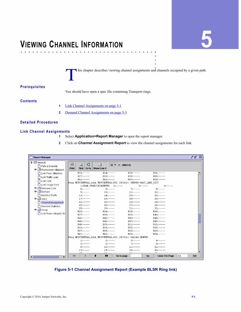
Link Channel Assignments1 Select Application>Report Manager to open the report manager.
2 Click on Channel Assignment Report to view the channel assignments for each link.
Figure 5-1 Channel Assignment Report (Example BLSR Ring link)
T
Copyright © 2014, Juniper Networks, Inc. 5-1
VI E W I N G C H A N N E L I N F O R M A T I O N5
This report shows how demands are assigned to different channels of the links.
R I N G L I N K F O R M A TFor a ring link, the report uses the following format:
Ring [RING_NAME], Link [LINK_NAME] ([LINK_TYPE]): [NODEA]-[NODEZ]
For example:
Ring MYRING,Link MYRING.R04 (STM16): NEWYORK-PHILADELPHIA
Following the first line is a section listing the channels that exist in the link and the demand that has been assigned to each channel. The channel type is listed to the left of each row. For an example, an SNCP ring link might look as follows:
STM1, 1:ckt196 , 2:ckt205 , 3:ckt208 , 4:ckt233 STM1, 5:ckt260 , 6:ckt34 , 7:ckt227 , 8:ckt238 STM1, 9:ckt241 , 10:ckt245 , 11:----- , 12:----- STM1, 13:----- , 14:----- , 15:----- , 16:-----
Note that rings with protection channels (e.g., BLSR/MS-SPR rings) will have a slightly different format. Some of the channels are prefixed with a ‘B’ which stands for backup, or protection channels. If the report is viewed under a failure simulation then some of the protection paths may be used for rerouted traffic. An example MS-SPR ring link might look as follows:
STM1, 1:ckt196 , 2:ckt205 , 3:ckt208 , 4:ckt233 STM1, 5:ckt260 , 6:ckt34 , 7:ckt227 , 8:ckt238 STM1, B9:ckt241 , B10:ckt245 , B11:----- , B12:----- STM1, B13:----- , B14:----- , B15:----- , B16:-----
M E S H L I N K F O R M A TThe following is an example of the format for an OC48 mesh link with one OC12 demand and 10 OC3 demands. Note that the numbering in this example is based on T3. As a result, the channel number skips from 1 to 13 in the first row because the OC12 demand occupied 12 T1 channels.
Link MESH33 (OC48): HALIFAX-BOSTON_MA OC12, 1:OC12dmd ,** ,** ,** , OC3, 13:IP_LINK_671,** ,** ,** , OC3, 16:IP_LINK_705,** ,** ,** , OC3, 19:IP_LINK_638,** ,** ,** , OC3, 22:IP_LINK_678,** ,** ,** , OC3, 25:IP_LINK_688,** ,** ,** , OC3, 28:IP_LINK_650,** ,** ,** , OC3, 31:IP_LINK_704,** ,** ,** , OC3, 34:IP_LINK_714,** ,** ,** , OC3, 37:IP_LINK_714,** ,** ,** , OC3, 40:IP_LINK_714,** ,** ,** , T3, 43:- ,** ,** ,** ,
T3, 44:- ,** ,** ,** ,T3, 45:- ,** ,** ,** ,T3, 46:- ,** ,** ,** ,T3, 47:- ,** ,** ,** ,T3, 48:- ,** ,** ,** ,
5-2 Copyright © 2014, Juniper Networks, Inc.
VI E W I N G C H A N N E L I N F O R M A T I O N
. . . . .
L I N K W I N D O W C A P A C I T Y T A B3 Channel assignments can also be seen from the link window Capacity tab in View or Design mode.
Each channel will have a number and will either have a demand routed over it or it will be empty.
Figure 5-2 Channel Information
Demand Channel AssignmentsIn addition to links, channel information is also displayed for demands.
4 To see what channels a demand is routed over, select the Path & Diversity Report.
Figure 5-3 Path & Diversity Report
For each demand, under the Actual_Path column, each link is displayed followed by channel of that link that the demand used. For example, LINK1.CH1-LINK0.CH1 indicates that the demand used channel 1 on link1 and channel 1 on link0.
Copyright © 2014, Juniper Networks, Inc. 5-3
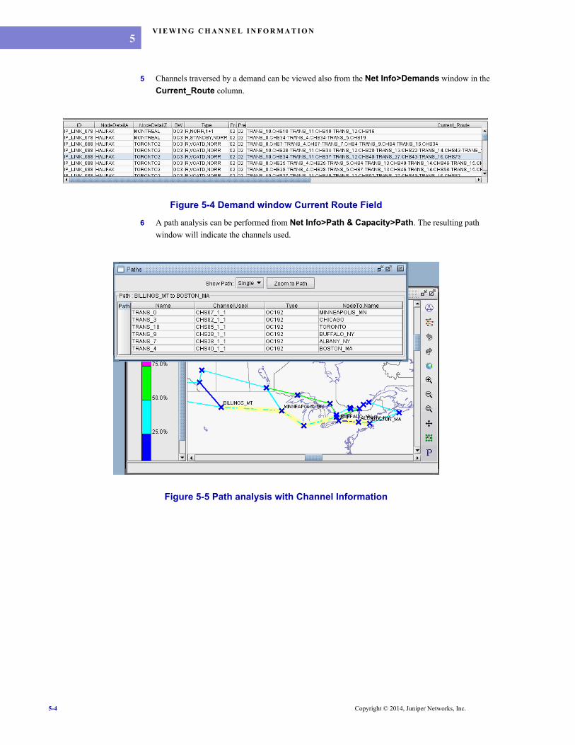
VI E W I N G C H A N N E L I N F O R M A T I O N5
5 Channels traversed by a demand can be viewed also from the Net Info>Demands window in the
Current_Route column.
Figure 5-4 Demand window Current Route Field
6 A path analysis can be performed from Net Info>Path & Capacity>Path. The resulting path
window will indicate the channels used.
Figure 5-5 Path analysis with Channel Information
5-4 Copyright © 2014, Juniper Networks, Inc.
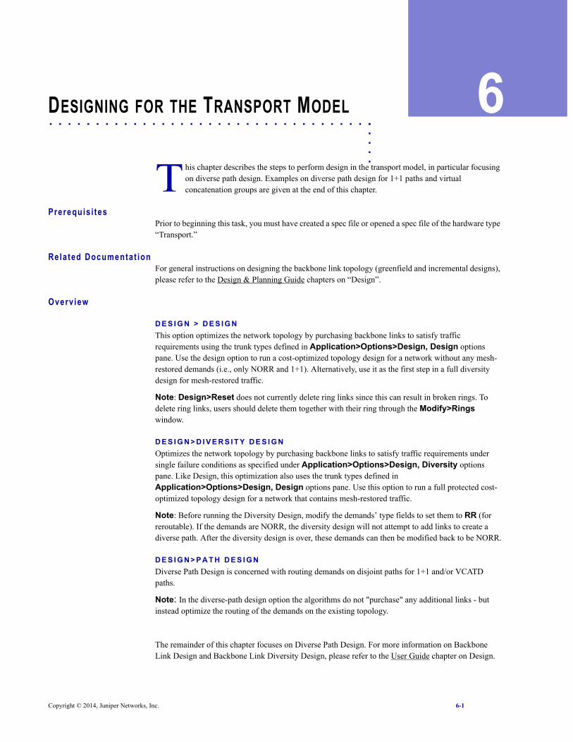
. . . . .
. . . . . . . . . . . . . . . . . . . . . . . . . . . . . . . . . . .DESIGNING FOR THE TRANSPORT MODEL 6
his chapter describes the steps to perform design in the transport model, in particular focusing on diverse path design. Examples on diverse path design for 1+1 paths and virtual concatenation groups are given at the end of this chapter.
Prerequis i tesPrior to beginning this task, you must have created a spec file or opened a spec file of the hardware type “Transport.”
Related Documentat ionFor general instructions on designing the backbone link topology (greenfield and incremental designs), please refer to the Design & Planning Guide chapters on “Design”.
Overv iew
D E S I G N > D E S I G NThis option optimizes the network topology by purchasing backbone links to satisfy traffic requirements using the trunk types defined in Application>Options>Design, Design options pane. Use the design option to run a cost-optimized topology design for a network without any mesh-restored demands (i.e., only NORR and 1+1). Alternatively, use it as the first step in a full diversity design for mesh-restored traffic.
Note: Design>Reset does not currently delete ring links since this can result in broken rings. To delete ring links, users should delete them together with their ring through the Modify>Rings window.
D E S I G N > D I V E R S I T Y D E S I G NOptimizes the network topology by purchasing backbone links to satisfy traffic requirements under single failure conditions as specified under Application>Options>Design, Diversity options pane. Like Design, this optimization also uses the trunk types defined in Application>Options>Design, Design options pane. Use this option to run a full protected cost-optimized topology design for a network that contains mesh-restored traffic.
Note: Before running the Diversity Design, modify the demands’ type fields to set them to RR (for reroutable). If the demands are NORR, the diversity design will not attempt to add links to create a diverse path. After the diversity design is over, these demands can then be modified back to be NORR.
D E S I G N > P A T H D E S I G NDiverse Path Design is concerned with routing demands on disjoint paths for 1+1 and/or VCATD paths.
Note: In the diverse-path design option the algorithms do not "purchase" any additional links - but instead optimize the routing of the demands on the existing topology.
The remainder of this chapter focuses on Diverse Path Design. For more information on Backbone Link Design and Backbone Link Diversity Design, please refer to the User Guide chapter on Design.
T
Copyright © 2014, Juniper Networks, Inc. 6-1
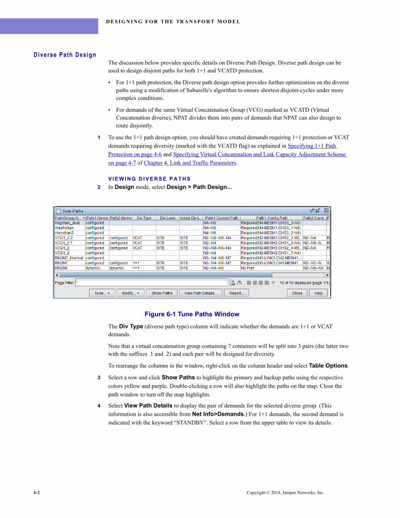
D E S I G N I N G F O R T H E TR A N S P O R T M O D E L
Diverse Path DesignThe discussion below provides specific details on Diverse Path Design. Diverse path design can be used to design disjoint paths for both 1+1 and VCATD protection.
• For 1+1 path protection, the Diverse path design option provides further optimization on the diverse paths using a modification of Suburelle's algorithm to ensure shortest disjoint-cycles under more complex conditions.
• For demands of the same Virtual Concatenation Group (VCG) marked as VCATD (Virtual Concatenation diverse), NPAT divides them into pairs of demands that NPAT can also design to route disjointly.
1 To use the 1+1 path design option, you should have created demands requiring 1+1 protection or VCAT
demands requiring diversity (marked with the VCATD flag) as explained in Specifying 1+1 Path
Protection on page 4-6 and Specifying Virtual Concatenation and Link Capacity Adjustment Scheme
on page 4-7 of Chapter 4, Link and Traffic Parameters.
V I E W I N G D I V E R S E P A T H S2 In Design mode, select Design > Path Design...
Figure 6-1 Tune Paths Window
The Div Type (diverse path type) column will indicate whether the demands are 1+1 or VCAT demands.
Note that a virtual concatenation group containing 7 containers will be split into 3 pairs (the latter two with the suffixes .1 and .2) and each pair will be designed for diversity.
To rearrange the columns in the window, right-click on the column header and select Table Options.
3 Select a row and click Show Paths to highlight the primary and backup paths using the respective
colors yellow and purple. Double-clicking a row will also highlight the paths on the map. Close the
path window to turn off the map highlights.
4 Select View Path Details to display the pair of demands for the selected diverse group. (This
information is also accessible from Net Info>Demands.) For 1+1 demands, the second demand is
indicated with the keyword “STANDBY”. Select a row from the upper table to view its details.
6-2 Copyright © 2014, Juniper Networks, Inc.
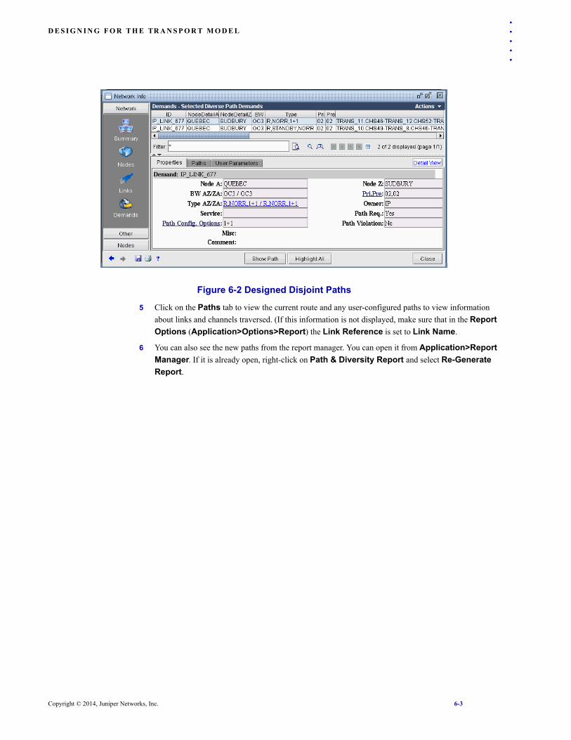
D E S I G N I N G F O R T H E TR A N S P O R T M O D E L
. . . . .
Figure 6-2 Designed Disjoint Paths
5 Click on the Paths tab to view the current route and any user-configured paths to view information
about links and channels traversed. (If this information is not displayed, make sure that in the Report Options (Application>Options>Report) the Link Reference is set to Link Name.
6 You can also see the new paths from the report manager. You can open it from Application>Report Manager. If it is already open, right-click on Path & Diversity Report and select Re-Generate Report.
Copyright © 2014, Juniper Networks, Inc. 6-3
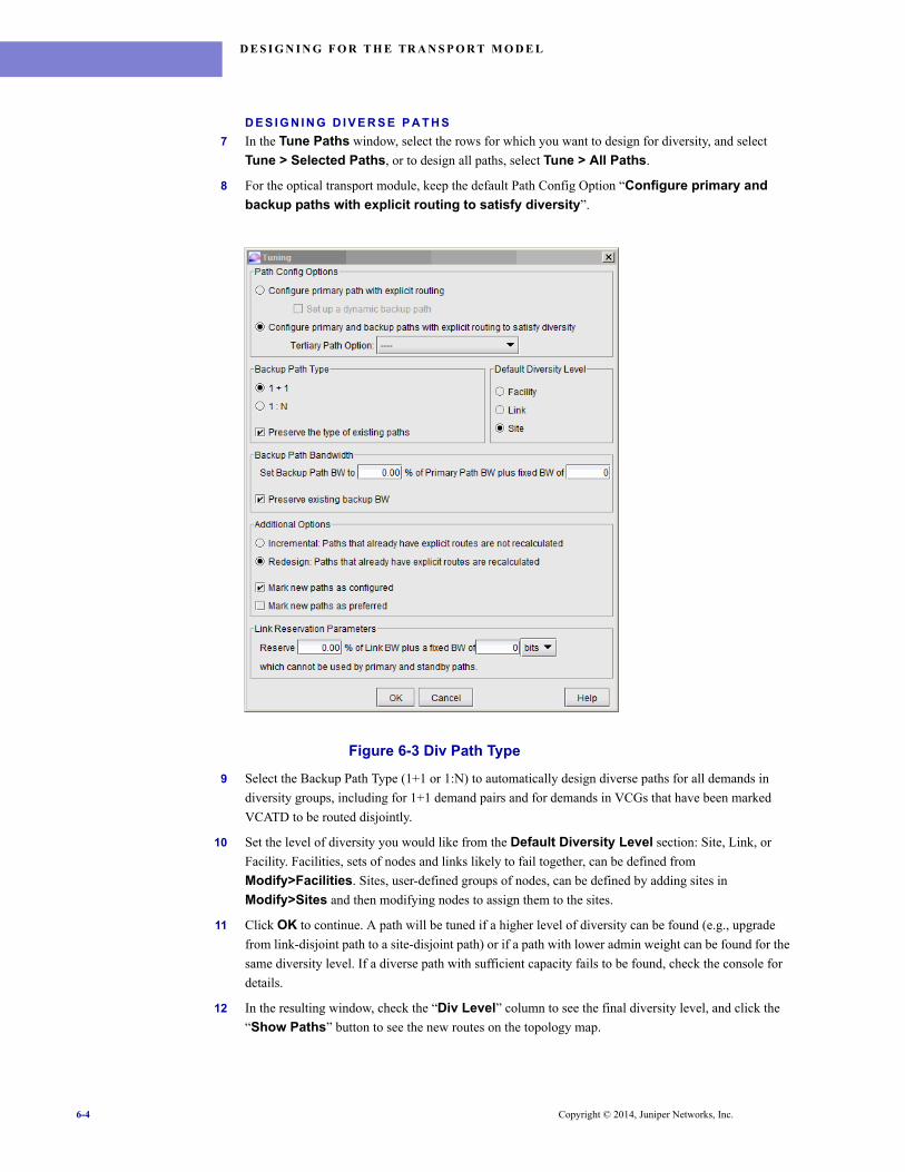
D E S I G N I N G F O R T H E TR A N S P O R T M O D E L
D E S I G N I N G D I V E R S E P A T H S7 In the Tune Paths window, select the rows for which you want to design for diversity, and select
Tune > Selected Paths, or to design all paths, select Tune > All Paths.
8 For the optical transport module, keep the default Path Config Option “Configure primary and backup paths with explicit routing to satisfy diversity”.
Figure 6-3 Div Path Type
9 Select the Backup Path Type (1+1 or 1:N) to automatically design diverse paths for all demands in
diversity groups, including for 1+1 demand pairs and for demands in VCGs that have been marked
VCATD to be routed disjointly.
10 Set the level of diversity you would like from the Default Diversity Level section: Site, Link, or
Facility. Facilities, sets of nodes and links likely to fail together, can be defined from
Modify>Facilities. Sites, user-defined groups of nodes, can be defined by adding sites in
Modify>Sites and then modifying nodes to assign them to the sites.
11 Click OK to continue. A path will be tuned if a higher level of diversity can be found (e.g., upgrade
from link-disjoint path to a site-disjoint path) or if a path with lower admin weight can be found for the
same diversity level. If a diverse path with sufficient capacity fails to be found, check the console for
details.
12 In the resulting window, check the “Div Level” column to see the final diversity level, and click the
“Show Paths” button to see the new routes on the topology map.
6-4 Copyright © 2014, Juniper Networks, Inc.
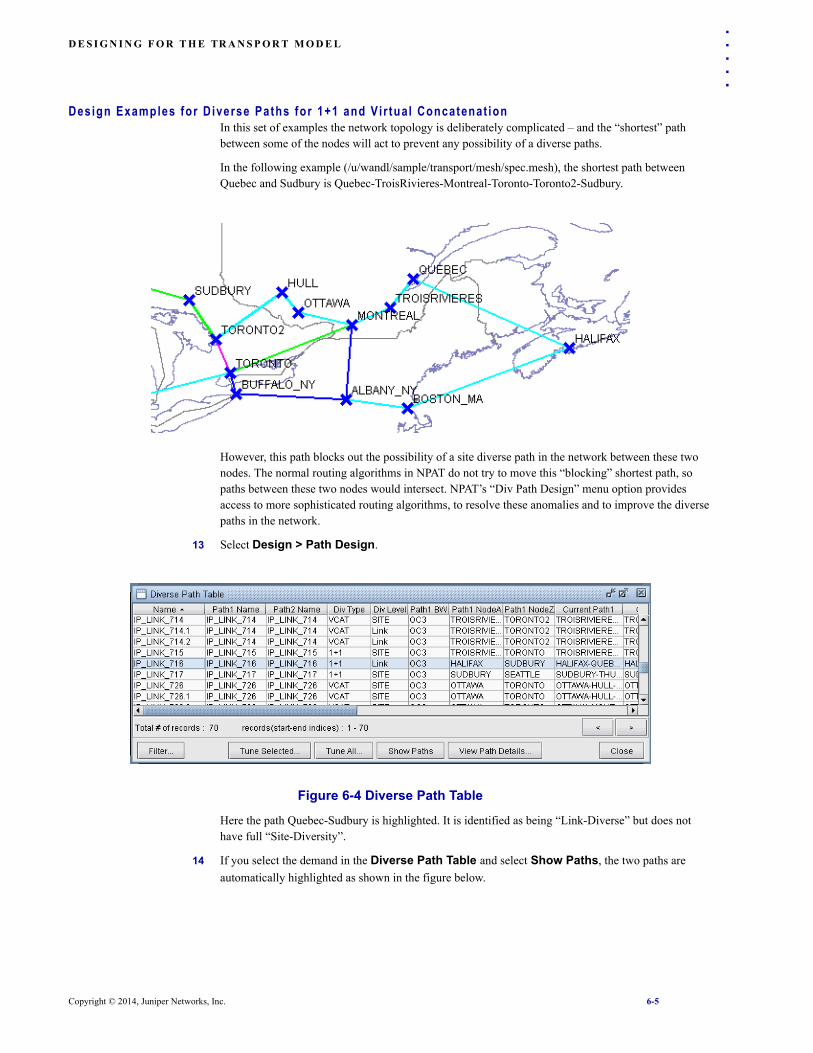
D E S I G N I N G F O R T H E TR A N S P O R T M O D E L
. . . . .
Design Examples for D iverse Paths for 1+1 and Vi r tual Concatenat ionIn this set of examples the network topology is deliberately complicated – and the “shortest” path between some of the nodes will act to prevent any possibility of a diverse paths.
In the following example (/u/wandl/sample/transport/mesh/spec.mesh), the shortest path between Quebec and Sudbury is Quebec-TroisRivieres-Montreal-Toronto-Toronto2-Sudbury.
However, this path blocks out the possibility of a site diverse path in the network between these two nodes. The normal routing algorithms in NPAT do not try to move this “blocking” shortest path, so paths between these two nodes would intersect. NPAT’s “Div Path Design” menu option provides access to more sophisticated routing algorithms, to resolve these anomalies and to improve the diverse paths in the network.
13 Select Design > Path Design.
Figure 6-4 Diverse Path Table
Here the path Quebec-Sudbury is highlighted. It is identified as being “Link-Diverse” but does not have full “Site-Diversity”.
14 If you select the demand in the Diverse Path Table and select Show Paths, the two paths are
automatically highlighted as shown in the figure below.
Copyright © 2014, Juniper Networks, Inc. 6-5
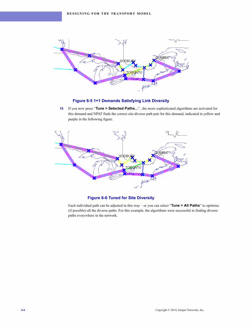
D E S I G N I N G F O R T H E TR A N S P O R T M O D E L
Figure 6-5 1+1 Demands Satisfying Link Diversity
15 If you now press “Tune > Selected Paths...” , the more sophisticated algorithms are activated for
this demand and NPAT finds the correct site-diverse path pair for this demand, indicated in yellow and
purple in the following figure.
Figure 6-6 Tuned for Site Diversity
Each individual path can be adjusted in this way – or you can select “Tune > All Paths” to optimise (if possible) all the diverse paths. For this example, the algorithms were successful in finding diverse paths everywhere in the network.
6-6 Copyright © 2014, Juniper Networks, Inc.
D E S I G N I N G F O R T H E TR A N S P O R T M O D E L
. . . . .
“Vir tual -Concatenat ion” Diverse (VCATD) Paths and Div Path DesignVirtual concatenation is a mechanism to associate a link in an IP network with a group of links on the transport layer carrying it. In the following example the OC12 links for the IP network were “Upgraded” to Gigabit-Ethernet. These are then each carried on the transport network as 7xOC3 demands. NPAT’s VCATD setting will group links within the same virtual concatenation group into pairs – and attempt to route each pair diversely from each other.
The same issues of path-diversity arise for groups of links routed diversely in pairs as for 1+1 protection. Again NPAT’s normal routing algorithms will not necessarily find diverse paths in this situation, even though the network may allow it. As for 1+1 protected demands the Div Path Design option will allow the user to improve the diversity of such paths .
16 The figure below from the Demands window indicates a mixture of 1+1 protected OC3’s and
Gigabit-Ethernet links grouped as 7 OC3 demands over the transport layer.
Figure 6-7 VCATD Demand Entries for Gigabit Ethernet from Halifax toToronto2
17 Selecting Tune > Selected Paths from the Diverse Path Table window results in the figure
shown below. The 7 demands from Halifax to Toronto2 are displayed as 3 pairs, each requiring
diversity from its associate. In this way the transport network resources are used more efficiently – as
capacity does not need to be reserved for protection. If some of the OC3’s carrying the Gigabit-
Ethernet link were to fail then only part of the capacity of the link would be lost – but the connectivity
in the IP layer would be maintained.
Figure 6-8 Diverse Table indicating pairs within VCATD group
Copyright © 2014, Juniper Networks, Inc. 6-7
D E S I G N I N G F O R T H E TR A N S P O R T M O D E L
18 The last demand pair from Halifax to Toronto2 has demands that are link diverse as indicated in the
Div. Level column. Select IP_LINK_688.2 and click “Show Paths” to highlight the link diverse
paths.
Figure 6-9 Link-Diverse Paths Crossing for VCATD pair
19 Select Tune > Selected Paths... to obtain the following site-diverse paths.
Figure 6-10 Site-Diverse Paths Found By Tuning
As with 1+1 demands, each pair requiring diversity can be adjusted in this way, or you can press “Tune > All Paths” to optimize (if possible) all the diverse paths.
6-8 Copyright © 2014, Juniper Networks, Inc.
D E S I G N I N G F O R T H E TR A N S P O R T M O D E L
. . . . .
20 After performing diverse path design, the results can also be viewed from the Path & DiversityReport of the Report Manager (Applications>Report Manager) shown below.
Figure 6-11 Path & Diversity Report
The DivGroup column of this report indicates which channels of the VCG were paired to satisfy diversity requirements and the highest level of diversity achieved. The pairing is indicated using group names like IP_LINK_688.2 that have a number appended to the end of the VCG to indicate the pair number.
Copyright © 2014, Juniper Networks, Inc. 6-9

D E S I G N I N G F O R T H E TR A N S P O R T M O D E L
6-10 Copyright © 2014, Juniper Networks, Inc.
. . . . .
. . . . . . . . . . . . . . . . . . . . . . . . . . . . . . . . . . .FAILURE SIMULATION 7
his chapter describes the steps to perform failure simulation. Failing individual components on a network allows the user to see how demands are rerouted across a network on particular failure conditions. Using failure simulation is a good way of showing how demands are
rerouted under failure conditions with the various network topologies and protection options. Each ring type and the various mesh protection options reroutes (or drops) traffic in different ways. All the general types of protection of topology are covered in this section.
Prerequis i tesPrior to beginning this task, you must have created a spec file or opened a spec file as described in the Design & Planning Guide. More specifically, the network model must be of the hardware type “Transport” in order for these features to be available.
Related Documentat ionFor general instructions on performing a failure simulation, please refer to the Design & Planning Guide chapter on Simulation.
For information on multilayer simulations, refer to Chapter 8, Multi-Layer Analysis.
Overv iewFailure simulations can be performed in two ways. The first is to fail individual components (nodes, links, and shared risk link groups (facilities)) and run a failure simulation. The second is to run a failure simulation script such as an exhaustive failure simulation on all the components in the network or an up-down sequence. The following document provides examples of failure simulation in the following cases:
• UPSR ring failure
• BLSR ring failure
• Failure over multiple rings
• Mesh restoration
• 1+1 path protection
T
Copyright © 2014, Juniper Networks, Inc. 7-1
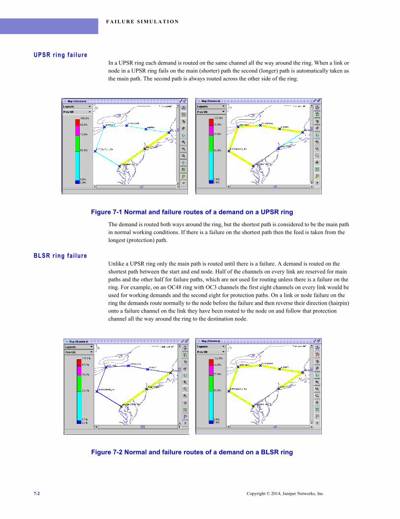
F A I L U R E S I M U L A T I O N
UPSR r ing fa i lureIn a UPSR ring each demand is routed on the same channel all the way around the ring. When a link or node in a UPSR ring fails on the main (shorter) path the second (longer) path is automatically taken as the main path. The second path is always routed across the other side of the ring.
Figure 7-1 Normal and failure routes of a demand on a UPSR ring
The demand is routed both ways around the ring, but the shortest path is considered to be the main path in normal working conditions. If there is a failure on the shortest path then the feed is taken from the longest (protection) path.
BLSR r ing fa i lureUnlike a UPSR ring only the main path is routed until there is a failure. A demand is routed on the shortest path between the start and end node. Half of the channels on every link are reserved for main paths and the other half for failure paths, which are not used for routing unless there is a failure on the ring. For example, on an OC48 ring with OC3 channels the first eight channels on every link would be used for working demands and the second eight for protection paths. On a link or node failure on the ring the demands route normally to the node before the failure and then reverse their direction (hairpin) onto a failure channel on the link they have been routed to the node on and follow that protection channel all the way around the ring to the destination node.
Figure 7-2 Normal and failure routes of a demand on a BLSR ring
7-2 Copyright © 2014, Juniper Networks, Inc.
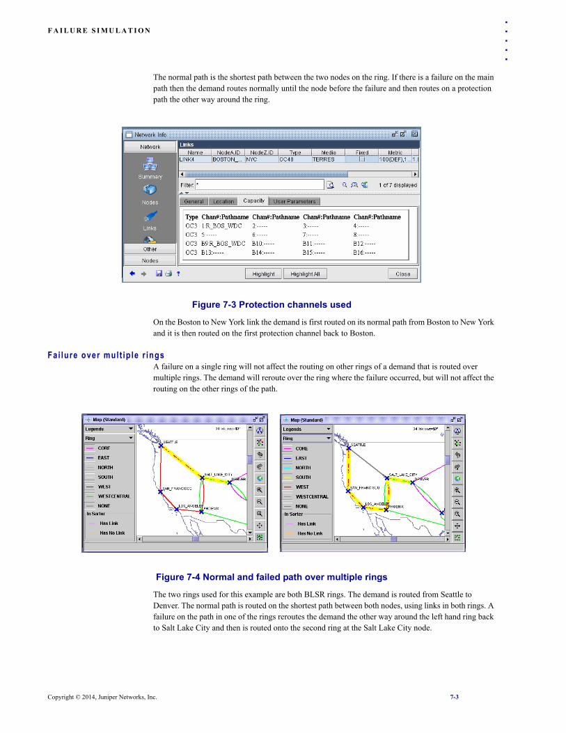
F A I L U R E S I M U L A T I O N
. . . . .
The normal path is the shortest path between the two nodes on the ring. If there is a failure on the main path then the demand routes normally until the node before the failure and then routes on a protection path the other way around the ring.Figure 7-3 Protection channels used
On the Boston to New York link the demand is first routed on its normal path from Boston to New York and it is then routed on the first protection channel back to Boston.
Fai lure over mul t ip le r ingsA failure on a single ring will not affect the routing on other rings of a demand that is routed over multiple rings. The demand will reroute over the ring where the failure occurred, but will not affect the routing on the other rings of the path.
Figure 7-4 Normal and failed path over multiple rings
The two rings used for this example are both BLSR rings. The demand is routed from Seattle to Denver. The normal path is routed on the shortest path between both nodes, using links in both rings. A failure on the path in one of the rings reroutes the demand the other way around the left hand ring back to Salt Lake City and then is routed onto the second ring at the Salt Lake City node.
Copyright © 2014, Juniper Networks, Inc. 7-3
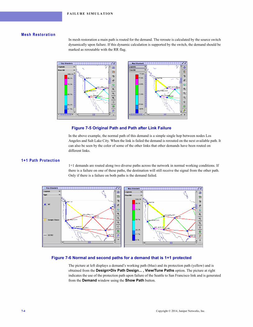
F A I L U R E S I M U L A T I O N
Mesh Restorat ionIn mesh restoration a main path is routed for the demand. The reroute is calculated by the source switch dynamically upon failure. If this dynamic calculation is supported by the switch, the demand should be marked as reroutable with the RR flag.
Figure 7-5 Original Path and Path after Link Failure
In the above example, the normal path of this demand is a simple single hop between nodes Los Angeles and Salt Lake City. When the link is failed the demand is rerouted on the next available path. It can also be seen by the color of some of the other links that other demands have been routed on different links.
1+1 Path Protect ion1+1 demands are routed along two diverse paths across the network in normal working conditions. If there is a failure on one of these paths, the destination will still receive the signal from the other path. Only if there is a failure on both paths is the demand failed.
Figure 7-6 Normal and second paths for a demand that is 1+1 protected
The picture at left displays a demand’s working path (blue) and its protection path (yellow) and is obtained from the Design>Div Path Design... , View/Tune Paths option. The picture at right indicates the use of the protection path upon failure of the Seattle to San Francisco link and is generated from the Demand window using the Show Path button.
7-4 Copyright © 2014, Juniper Networks, Inc.

. . . . .
. . . . . . . . . . . . . . . . . . . . . . . . . . . . . . . . . . .MULTI-LAYER ANALYSIS 8
his chapter discusses detailed analysis, reporting, and failure simulations across multiple network layers. The end of this chapter contains an example of how a failure simulation at the transport layer can provide information for the client layer.
Overv iewA typical network architecture for major carriers is shown schematically in the diagram below.
Figure 8-1 Multi-Layer Network Architecture
In this example the transport network is responsible for carrying the PoS links for the carrier’s IP Network, which provides services directly to the customers. A more typical situation is where the transport network carries links for several of the carrier’s own networks (e.g. IP; ATM & Voice), as well as direct point-to-point services for large enterprise customers. This section will describe the operation in terms of an IP network for the client layer. However, the same set of analyses described in this section can of course be applied to more complex network structures in a similar manner.
Basic Requi rements for Mul t ip le-Layer AnalysisPrior to beginning this task, you must have created a spec file or opened a spec file as described in the Design & Planning Guide. More specifically, the network model must be of the hardware type “Transport” in order for these features to be available. In order to perform multi-layer analysis the user must have access to the appropriate network modules in NPAT or IP/MPLSView to model the client network.
NPAT Transport can model the routing and re-routing under failure of the IP Layer links over the physical optical fiber. To do this, there must be an exact, 1 to 1 relationship between the PoS link names in the IP layer and the SDH/SONET demands carried on the transport network. There is a utility
T
Copyright © 2014, Juniper Networks, Inc. 8-1
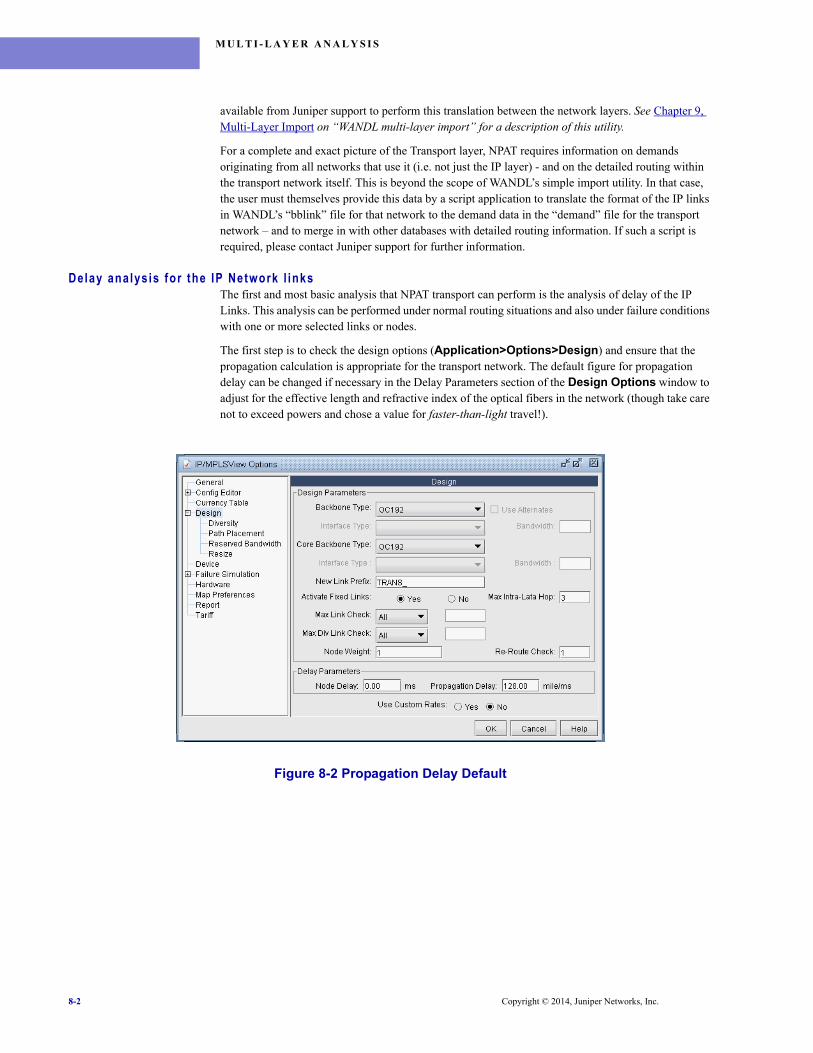
M U L T I - L A Y E R A N A L Y S I S
available from Juniper support to perform this translation between the network layers. See Chapter 9, Multi-Layer Import on “WANDL multi-layer import” for a description of this utility.
For a complete and exact picture of the Transport layer, NPAT requires information on demands originating from all networks that use it (i.e. not just the IP layer) - and on the detailed routing within the transport network itself. This is beyond the scope of WANDL’s simple import utility. In that case, the user must themselves provide this data by a script application to translate the format of the IP links in WANDL’s “bblink” file for that network to the demand data in the “demand” file for the transport network – and to merge in with other databases with detailed routing information. If such a script is required, please contact Juniper support for further information.
Delay analys is for the IP Network l inksThe first and most basic analysis that NPAT transport can perform is the analysis of delay of the IP Links. This analysis can be performed under normal routing situations and also under failure conditions with one or more selected links or nodes.
The first step is to check the design options (Application>Options>Design) and ensure that the propagation calculation is appropriate for the transport network. The default figure for propagation delay can be changed if necessary in the Delay Parameters section of the Design Options window to adjust for the effective length and refractive index of the optical fibers in the network (though take care not to exceed powers and chose a value for faster-than-light travel!).
Figure 8-2 Propagation Delay Default
8-2 Copyright © 2014, Juniper Networks, Inc.
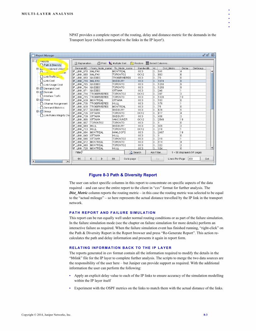
M U L T I - L A Y E R A N A L Y S I S
. . . . .
NPAT provides a complete report of the routing, delay and distance-metric for the demands in the Transport layer (which correspond to the links in the IP layer!).Figure 8-3 Path & Diversity Report
The user can select specific columns in this report to concentrate on specific aspects of the data required – and can save the entire report to the client in “csv” format for further analysis. The Dist_Metric column reports the routing metric – in this case the routing metric was selected to be equal to the “actual mileage” – so here represents the actual distance travelled by the IP link in the transport network.
P A T H R E P O R T A N D F A I L U R E S I M U L A T I O NThis report can be run equally well under normal routing conditions or as part of the failure simulation. In the failure simulation mode (see the chapter on failure simulation for more details) perform an interactive failure as required. When the failure simulation event has finished running, “right-click” on the Path & Diversity Report in the Report browser and press “Re-Generate Report”. This action re-calculates the path and delay information and presents it again in report form.
R E L A T I N G I N F O R M A T I O N B A C K T O T H E I P L A Y E RThe reports generated in csv format contain all the information required to modify the details in the “bblink” file for the IP layer to complete further analysis. The scripts to merge the two data sources are the responsibility of the user here – but Juniper can provide support as required. With the additional information the user can perform the following:
• Apply an explicit delay value to each of the IP links to ensure accuracy of the simulation modelling within the IP layer itself
• Experiment with the OSPF metrics on the links to match them with the actual distance of the links.
Copyright © 2014, Juniper Networks, Inc. 8-3
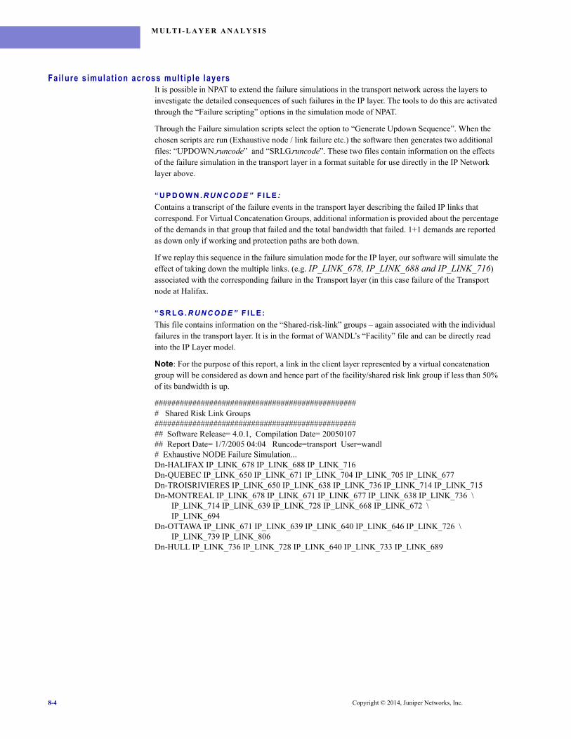
M U L T I - L A Y E R A N A L Y S I S
Fai lure s imulat ion across mul t ip le layersIt is possible in NPAT to extend the failure simulations in the transport network across the layers to investigate the detailed consequences of such failures in the IP layer. The tools to do this are activated through the “Failure scripting” options in the simulation mode of NPAT.
Through the Failure simulation scripts select the option to “Generate Updown Sequence”. When the chosen scripts are run (Exhaustive node / link failure etc.) the software then generates two additional files: “UPDOWN.runcode” and “SRLG.runcode”. These two files contain information on the effects of the failure simulation in the transport layer in a format suitable for use directly in the IP Network layer above.
“ U P D O W N .RUNCODE” F I L E :Contains a transcript of the failure events in the transport layer describing the failed IP links that correspond. For Virtual Concatenation Groups, additional information is provided about the percentage of the demands in that group that failed and the total bandwidth that failed. 1+1 demands are reported as down only if working and protection paths are both down.
If we replay this sequence in the failure simulation mode for the IP layer, our software will simulate the effect of taking down the multiple links. (e.g. IP_LINK_678, IP_LINK_688 and IP_LINK_716) associated with the corresponding failure in the Transport layer (in this case failure of the Transport node at Halifax.
“ S R L G .RUNCODE” F I L E : This file contains information on the “Shared-risk-link” groups – again associated with the individual failures in the transport layer. It is in the format of WANDL’s “Facility” file and can be directly read into the IP Layer model.
Note: For the purpose of this report, a link in the client layer represented by a virtual concatenation group will be considered as down and hence part of the facility/shared risk link group if less than 50% of its bandwidth is up.
################################################# Shared Risk Link Groups ################################################## Software Release= 4.0.1, Compilation Date= 20050107## Report Date= 1/7/2005 04:04 Runcode=transport User=wandl# Exhaustive NODE Failure Simulation...Dn-HALIFAX IP_LINK_678 IP_LINK_688 IP_LINK_716 Dn-QUEBEC IP_LINK_650 IP_LINK_671 IP_LINK_704 IP_LINK_705 IP_LINK_677 Dn-TROISRIVIERES IP_LINK_650 IP_LINK_638 IP_LINK_736 IP_LINK_714 IP_LINK_715 Dn-MONTREAL IP_LINK_678 IP_LINK_671 IP_LINK_677 IP_LINK_638 IP_LINK_736 \
IP_LINK_714 IP_LINK_639 IP_LINK_728 IP_LINK_668 IP_LINK_672 \IP_LINK_694
Dn-OTTAWA IP_LINK_671 IP_LINK_639 IP_LINK_640 IP_LINK_646 IP_LINK_726 \IP_LINK_739 IP_LINK_806
Dn-HULL IP_LINK_736 IP_LINK_728 IP_LINK_640 IP_LINK_733 IP_LINK_689
8-4 Copyright © 2014, Juniper Networks, Inc.
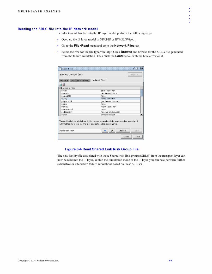
M U L T I - L A Y E R A N A L Y S I S
. . . . .
Reading the SRLG f i le in to the IP Network modelIn order to read this file into the IP layer model perform the following steps:
• Open up the IP layer model in NPAT-IP or IP/MPLSView.
• Go to the File>Read menu and go to the Network Files tab
• Select the row for the file type “facility.” Click Browse and browse for the SRLG file generated from the failure simulation. Then click the Load button with the blue arrow on it.
Figure 8-4 Read Shared Link Risk Group File
The new facility file associated with these Shared-risk-link-groups (SRLG) from the transport layer can now be read into the IP layer. Within the Simulation mode of the IP layer you can now perform further exhaustive or interactive failure simulations based on these SRLG’s.
Copyright © 2014, Juniper Networks, Inc. 8-5
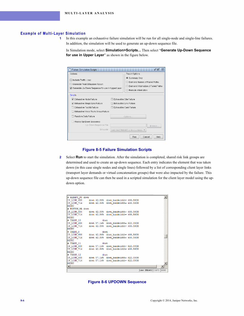
M U L T I - L A Y E R A N A L Y S I S
Example of Mul t i -Layer S imulat ion1 In this example an exhaustive failure simulation will be run for all single-node and single-line failures.
In addition, the simulation will be used to generate an up-down sequence file.
In Simulation mode, select Simulation>Scripts... Then select “Generate Up-Down Sequence for use in Upper Layer” as shown in the figure below.
Figure 8-5 Failure Simulation Scripts
2 Select Run to start the simulation. After the simulation is completed, shared risk link groups are
determined and used to create an up-down sequence. Each entry indicates the element that was taken
down (in this case single nodes and single lines) followed by a list of corresponding client layer links
(transport layer demands or virtual concatenation groups) that were also impacted by the failure. This
up-down sequence file can then be used in a scripted simulation for the client layer model using the up-
down option.
Figure 8-6 UPDOWN Sequence
8-6 Copyright © 2014, Juniper Networks, Inc.

M U L T I - L A Y E R A N A L Y S I S
. . . . .
The above file indicates that when the transport link TRANS_12 was taken down, this resulted in 57.14% (4 of the 7 channels) of the Virtual Concatenation Groups (VCGs) IP_LINK_688 and IP_LINK_714 to be taken down for a total down bandwidth of 622.080Mbps for both VCGs.3 The SRLG (Shared Risk Link Group) file is also created as a result of the simulation and can be opened
from the File Manager as displayed below. Based on the failure simulation, information is gathered
about which links of the IP layer (demands of the transport layer) will go down together due to a failure
on the transport layer. This facility file that can be used to run designs or simulations or facility-diverse
path designs on the client layer.
Figure 8-7 SRLG File
The following entry of the SRLG file indicates a shared risk link group (facility) of the name Dn-TRANS_12 containing the links IP_LINK_600 and IP_LINK_714.
Dn-TRANS_12 IP_LINK_600 IP_LINK_714
Entries containing only one link are commented out since a facility entry only needs to be created for facilities with more than one node/link.
Copyright © 2014, Juniper Networks, Inc. 8-7

M U L T I - L A Y E R A N A L Y S I S
8-8 Copyright © 2014, Juniper Networks, Inc.

. . . . .
. . . . . . . . . . . . . . . . . . . . . . . . . . . . . . . . . . .MULTI-LAYER IMPORT 9
his chapter details the procedures to import a multi-layer network. This information can also be found in the “Multi-Layer” section of the Network Data Import Wizard chapter of the General Reference Guide.
Prerequis i tes*While the import functionality is general, in order to run a specific multilayer model, the appropriate password license is required for each layer technology (e.g. ATM, ROUTER, etc.). Please contact your WANDL representative for more information.
Overv iewThe end-to-end demands in one layer of a network correlate to the links in the layer above it. Or to rephrase, the links in one layer of a network are often logical links that reflect the end-to-end demands in the layer below it. When importing multi-layer demands, the program will convert links in the Source Layer (e.g. ATM or IP layer) view of the network into demands that can be read in when analyzing the Destination Layer (e.g. SONET/SDH layer) view of the network.
Figure 9-1 Example of Multi-Layer View
For example, in Figure 9-1, the logical link from B1 to B2 in Source Layer (Layer 2) will be translated by the “Import Multi-Layer Demand” feature into a demand between A1 and A2 in the Destination Layer (Layer 1). Specific type or bandwidth translations between the two layers are handled by an optional Link Type Mapping File.
Also notice that a node mapping is often involved during the translation, and that many nodes in the Source Layer may correlate to the same node in the Destination Layer. This mapping is supported by the Import Multi-Layer Demand feature through the use of an optional Node Name Mapping File.
T
Copyright © 2014, Juniper Networks, Inc. 9-1
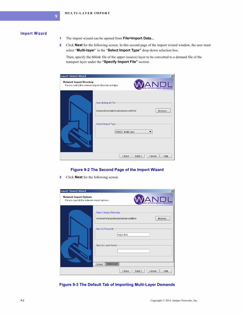
M U L T I - L A Y E R I M P O R T9
Import Wizard1 The import wizard can be opened from File>Import Data...
2 Click Next for the following screen. In this second page of the import wizard window, the user must
select “Multi-layer” in the “Select Import Type” drop-down selection box.
Then, specify the bblink file of the upper (source) layer to be converted to a demand file of the transport layer under the “Specify Import File” section.
Figure 9-2 The Second Page of the Import Wizard
3 Click Next for the following screen.
Figure 9-3 The Default Tab of Importing Multi-Layer Demands
9-2 Copyright © 2014, Juniper Networks, Inc.
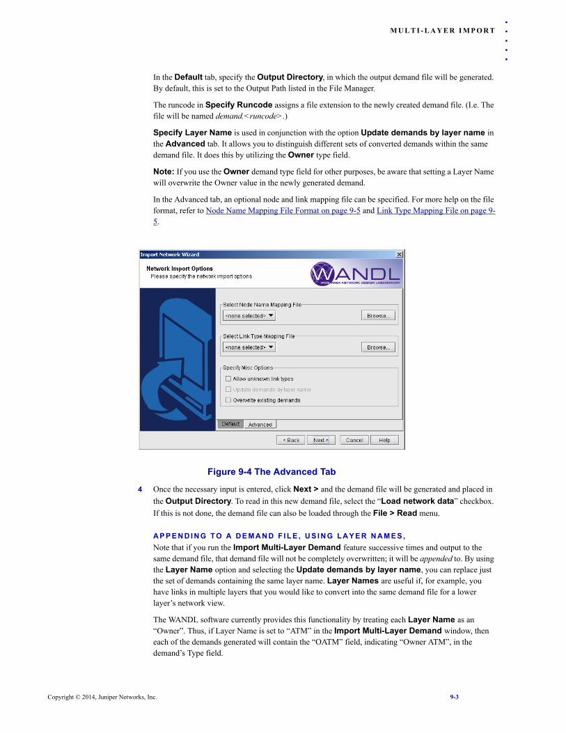
M U L T I - L A Y E R I M P O R T
. . . . .
In the Default tab, specify the Output Directory, in which the output demand file will be generated. By default, this is set to the Output Path listed in the File Manager.The runcode in Specify Runcode assigns a file extension to the newly created demand file. (I.e. The file will be named demand.<runcode>.)
Specify Layer Name is used in conjunction with the option Update demands by layer name in the Advanced tab. It allows you to distinguish different sets of converted demands within the same demand file. It does this by utilizing the Owner type field.
Note: If you use the Owner demand type field for other purposes, be aware that setting a Layer Name will overwrite the Owner value in the newly generated demand.
In the Advanced tab, an optional node and link mapping file can be specified. For more help on the file format, refer to Node Name Mapping File Format on page 9-5 and Link Type Mapping File on page 9-5.
Figure 9-4 The Advanced Tab
4 Once the necessary input is entered, click Next > and the demand file will be generated and placed in
the Output Directory. To read in this new demand file, select the “Load network data” checkbox.
If this is not done, the demand file can also be loaded through the File > Read menu.
A P P E N D I N G T O A D E M A N D F I L E , U S I N G L A Y E R N A M E S , Note that if you run the Import Multi-Layer Demand feature successive times and output to the same demand file, that demand file will not be completely overwritten; it will be appended to. By using the Layer Name option and selecting the Update demands by layer name, you can replace just the set of demands containing the same layer name. Layer Names are useful if, for example, you have links in multiple layers that you would like to convert into the same demand file for a lower layer’s network view.
The WANDL software currently provides this functionality by treating each Layer Name as an “Owner”. Thus, if Layer Name is set to “ATM” in the Import Multi-Layer Demand window, then each of the demands generated will contain the “OATM” field, indicating “Owner ATM”, in the demand’s Type field.
Copyright © 2014, Juniper Networks, Inc. 9-3
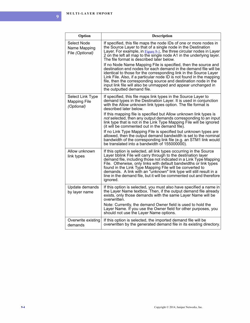
M U L T I - L A Y E R I M P O R T9
Option Description
Select Node Name Mapping File (Optional)
If specified, this file maps the node IDs of one or more nodes in the Source Layer to that of a single node in the Destination Layer. For example, in Figure 9-1, the three circular nodes in Layer 2 on the left all map to the single node A1 in the underlying layer. The file format is described later below.If no Node Name Mapping File is specified, then the source and destination end nodes for each demand in the demand file will be identical to those for the corresponding link in the Source Layer Link File. Also, if a particular node ID is not found in the mapping file, then the corresponding source and destination node in the input link file will also be unmapped and appear unchanged in the outputted demand file.
Select Link Type Mapping File (Optional)
If specified, this file maps link types in the Source Layer to demand types in the Destination Layer. It is used in conjunction with the Allow unknown link types option. The file format is described later below.If this mapping file is specified but Allow unknown link types is not selected, then any output demands corresponding to an input link type that is not in the Link Type Mapping File will be ignored (it will be commented out in the demand file).If no Link Type Mapping File is specified but unknown types are allowed, then the output demand bandwidth is set to the nominal bandwidth of the corresponding link file (e.g. an STM1 link would be translated into a bandwidth of 155000000).
Allow unknown link types
If this option is selected, all link types occurring in the Source Layer bblink File will carry through to the destination layer demand file, including those not indicated in a Link Type Mapping File. Otherwise, only links with default bandwidths or link types found in the Link Type Mapping File will be converted to demands. A link with an "unknown" link type will still result in a line in the demand file, but it will be commented out and therefore ignored.
Update demands by layer name
If this option is selected, you must also have specified a name in the Layer Name textbox. Then, if the output demand file already exists, only those demands with the same Layer Name will be overwritten.Note: Currently, the demand Owner field is used to hold the Layer Name. If you use the Owner field for other purposes, you should not use the Layer Name options.
Overwrite existing demands
If this option is selected, the imported demand file will be overwritten by the generated demand file in its existing directory.
9-4 Copyright © 2014, Juniper Networks, Inc.
M U L T I - L A Y E R I M P O R T
. . . . .
N O D E N A M E M A P P I N G F I L E F O R M A TThis file maps one or more nodes in the Source Layer to a single node in the Destination Layer. Its file format is similar to that of the Site File. Specify the node using Node ID.DestLayer_Node SrcLayerNode1 [SrcLayerNode2...SrcLayerNodeN]
Example Mapping File:
A1 B1 B6 B8
A2 B2
L I N K T Y P E M A P P I N G F I L EThis file maps link types in the Source Layer to demand types in the Destination Layer. It can also be used to specify the Type fields for the correlated demands, as well as the Priority, Preemption. The Type fields should be comma-separated, just as they appear in the demand file. For more information on the Type and Priority, Preemption fields, please refer to the demand file format in the File Format Guide.
LinkType(BW) DemandType(BW) TypeFields Priority,Preemption
Example Mapping File:
OC3 STM1 R,A2Z 2,2
E X A M P L E C O N V E R S I O NThe following shows the basic input and output after converting a bblink file to a demand file using the Node Name Mapping File and Link Type Mapping File examples in the previous sections.
Input bblink file:
L1 B6 B2 DEF 1 OC3
Output demand file:
L1 A1 A2 STM1 R,A2Z 2,2
Copyright © 2014, Juniper Networks, Inc. 9-5

M U L T I - L A Y E R I M P O R T9
9-6 Copyright © 2014, Juniper Networks, Inc.