warping indexes with envelope transforms for query by humming
TRANSCRIPT

Warping Indexes with Envelope Transforms for Query byHumming ∗
Yunyue ZhuDepartment of Computer Science
Courant Institute of Mathematical SciencesNew York University, New York, NY 10012
Dennis ShashaDepartment of Computer Science
Courant Institute of Mathematical SciencesNew York University, New York, NY 10012
ABSTRACTA Query by Humming system allows the user to find a songby humming part of the tune. No musical training is needed.Previous query by humming systems have not provided sat-isfactory results for various reasons. Some systems havelow retrieval precision because they rely on melodic con-tour information from the hum tune, which in turn relies onthe error-prone note segmentation process. Some systemsyield better precision when matching the melody directlyfrom audio, but they are slow because of their extensiveuse of Dynamic Time Warping (DTW). Our approach im-proves both the retrieval precision and speed compared toprevious approaches. We treat music as a time series andexploit and improve well-developed techniques from time se-ries databases to index the music for fast similarity queries.We improve on existing DTW indexes technique by intro-ducing the concept of envelope transforms, which gives ageneral guideline for extending existing dimensionality re-duction methods to DTW indexes. The net result is highscalability. We confirm our claims through extensive exper-iments.
1. INTRODUCTIONYou have a tune lingering in your head for many days, butyou don’t know where you heard this tune or which song it isfrom. You can’t search it using an online search engine suchas Google because you know nothing about the metadataof the tune. Often, a music store clerk acts as a musicalsearch engine, interpreting tunes hummed by shoppers anddirecting them to an album. This works even for shopperswho can’t hum very well, as the authors know from personalexperience. Such a resource is very useful but hard to find.
A Query by Humming system is just such a resource. Theuser will hum a piece of tune into a microphone connected to
∗Work supported in part by U.S. NSF grants IIS-9988636and N2010-0115586.
Permission to make digital or hard copies of all or part of this work forpersonal or classroom use is granted without fee provided that copies arenot made or distributed for profit or commercial advantage and that copiesbear this notice and the full citation on the first page. To copy otherwise, orrepublish, to post on servers or to redistribute to lists, requires prior specificpermission and/or a fee.SIGMOD 2003, June 9-12, 2003, San Diego, CA.Copyright 2003 ACM 1-58113-634-X/03/06...$5.00.
a computer. The computer will search a database of tunesto find a list of melodies that are most similar to the user’s“query”. The user will then listen to this result to see if itis actually the tune that he had in mind. Sometimes theuser won’t get the tune he wanted because he hummed wayoff tune, the database does not contain that tune, or thecomputer is not intelligent enough to tell whether two tunessound similar.
Query by humming is a particular case of “Query by Con-tent” in multimedia databases. One queries a symbolicdatabase of melodies (such as MIDIs or digital music scores),rather than a general acoustic database (such as MP3s). Al-though these two formats can be linked by metadata such asartist and song names, there is no known method to extractmelodies from MP3. Querying acoustic databases [31] is aninteresting problem, but it is not the focus of a query byhumming system. Most research into “query by humming”in the multimedia research community uses the notion of“Contour” information. Melodic contour is the sequence ofrelative differences in pitch between successive notes [8]. Ithas been shown to be a method that the listeners use to de-termine similarities between melodies. However, the inher-ent difficulty the contour method encounters is that there isno known algorithm that can reliably transcribe the user’shumming to discrete notes. We discuss this point furtherbelow.
Recently, there has been work that matches a melody di-rectly from audio [19, 11, 34]. This generally gives betterquery results because it is free from the error-prone note seg-mentation. However, because such work relies on DynamicTime Warping (DTW), the performance is poor.
The database community has been investigating similarityquery in time series databases for a long time[1, 7]. Thispaper will show that query by humming is a natural applica-tion for time series database research. Time series databasetechniques, especially dynamic time warping indexes, canbe applied to build a fast and robust query by hummingdatabase system.
2. RELATED WORKMost of the research in pre-existing query by humming sys-tems uses pitch contour to match similar melodies [8, 5,20, 29]. The user’s humming is transcribed to a sequenceof discrete notes and the contour information is extracted

from the notes. This contour information is represented bya few letters. For example, (“U”, “D”, “S”) represents thata note is above, below or the same as the previous one. Nat-urally, more letters can be introduced to get a finer measureof the contour. For example, “u” indicates that a note isslightly higher than the previous one while “U” indicatesthat it is much higher. The tunes in the databases are alsorepresented by contour information. In this way, a pieceof melody is represented by a string with a small alphabet.The edit distance can be used to measure the similarity be-tween two melodies. Techniques for string matching suchas “q-grams” can be used to speed up the similarity query.The advantage of using contours is that while most users canhum the contour correctly, they cannot hum the contour in-tervals correctly. But such work suffers from two seriousproblems.
• It has been shown that contour information alone isnot enough to distinguish a large database of melodies.A typical query of six notes on a database of 2,697tracks would result in about 330 tracks being returned[28].
• It is very hard to segment a user’s humming into dis-crete notes. There are reliable algorithms to transcribethe user humming in each short time period to a spe-cific pitch [27]. But no good algorithm is known to seg-ment such a time series of pitches into discrete notes.The precision of the query system thus rests on animprecise preprocessing stage.
To avoid the first problem, one can use longer query lengthsand finer measures of contour intervals. But that requirestoo much of users, especially poor singers. The second prob-lem is more fundamental. There are two solutions proposedin the literature.
1. The user is required to clearly hum the notes of themelody using only the syllable “ta”, “la” or “da” [18,20]. But such an input method is very unnatural forusers. Moreover, when there are tie notes in a tune, itis very hard for the user to articulate them correctly.Such a cumbersome job should be left to intelligentcomputer programs.
2. Some recent work [19, 11, 34] proposes to match thequery directly from audio based on melody slope [34]or dynamic time warping [19, 11] to match the hum-query with the melodies in the music databases. Theresults reported using such methods are quite encour-aging. Compared to note based methods, such directmethods generally have higher retrieval precision [19].But this quality improvement comes at a price. Perfor-mance deteriorates to such an extent that [19] states“Perhaps the biggest criticism of our work is that itis clearly a brute-force approach and it is very slow.”No indices are used, which makes searching in a largemusic database unpractical.
The database community has been researching problems insimilarity query for time series databases for many years.
The techniques developed in the area might shed light onthe query by humming problem. Agrawal et al. [1] utilizedthe Discrete Fourier Transform (DFT) to transform datafrom the time domain into the frequency domain and used amultidimensional index structure to index the first few DFTcoefficients. The focus in their work was on whole sequencematching. This was generalized to allow subsequence match-ing [7, 21]. Rafiei and Mendelzon [25] improved this tech-nique by allowing transformations, including shifting, scal-ing and moving average, on the time series before similarityqueries. In addition to DFT [1, 25, 35], Discrete WaveletTransform (DWT) [6, 30, 23], Singular Value Decomposition(SVD)[16], Piecewise Aggregate Approximation (PAA)[32,13] and Adaptive Piecewise Constant Approximation [14]approaches have also been proposed for similarity search-ing.
Allowing Dynamic Time Warping (DTW) in time series sim-ilarity searching is very critical for a query by hummingsystem. A point-by-point distance measure between timeseries is very likely to fail due to variations in the durationof notes. Berndt and Clifford [4] introduced the concept ofDTW to the data mining community. They showed how touse Dynamic Programming to compute the DTW distanceand demonstrated its application as a time series similaritymeasure. Yi et al. [33] were the first to investigate the DTWin very large databases. They proposed two techniques tospeed up DTW in a pipeline fashion. The first technique isto use FastMap to index time series with the DTW distancemeasure. But this technique might result in false negatives.The second is a global lower-bounding technique for filteringout unlikely matches. In recent work, Keogh [13] proposeda technique for the exact indexing of DTW that guaranteesno false negatives.
2.1 Our contributionsIn this paper, we investigate the problem of indexing largemusic databases, which allows efficient and effective queryby humming. Our strategy and contributions are as follows.
• We treat both the melodies in the music databasesand the user humming input as time series. Such anapproach allows us to integrate many database index-ing techniques into a query by humming system, im-proving the quality of such system over the traditional(contour) string databases approach.
• We design an indexing scheme that is invariant to shift-ing, time scaling and local time warping. This makesthe system robust and allows flexible user humminginput, while attaining high speeds.
• We improve on the state-of-the-art indexing techniquefor time series databases allowing dynamic time warp-ing due to [13] by giving a better lower-bound distancefor dynamic time warping. This yields less false neg-atives and shows improvements of speed by 3 to 10times in practice.
• We formulate a general method for dimensionality re-duction transforms on time series envelopes. Existingdimensionality reduction transforms, such as DiscreteFourier Transform (DFT) and Discrete Wavelet Trans-form (DWT), can be extended to index time series

0
10
20
30
40
50
60
70
0 1 2 3 4 5 6 7 8 9 10 11
time (seconds)
pit
ch v
alu
es
Figure 1: An example of a pitch time series. It is thetune of the beginning two phrases in the Beatles’ssong “Hey Jude” hummed by an amateur.
allowing dynamic time warping while avoiding falsenegatives. This might have applications to video pro-cessing in the spirit of [13].
• The net effect is that our approach is scalable to largemusic databases, as we demonstrate.
3. ARCHITECTURE OF QUERY BY HUM-MING SYSTEM
A typical query by humming system includes three compo-nents:
• User humming: the input hum-query
• A database of music
• An index into the database for efficient retrieval of thehum-query
In this section, we will discuss these components in detail,with a focus on the indexing techniques.
3.1 User humming: the input hum-queryThe user hums the query melody using a PC microphonewith a single channel (mono). This acoustic input is seg-mented into frames of 10ms and each frame is resolved intoa pitch using a pitch tracking algorithm [27]. This resultsin a time series of the pitches. Figure 1 shows an exampleof a pitch time series. It is the tune of the first two phrasesin the Beatles’s song “Hey Jude”. The user may hum inany way he/she prefers. From the example of figure 1, wecan see that it is very hard for the human being to markthe borders between notes. This is also the case for thecomputer. As mentioned above, we are not aware of anyalgorithm or product that can automatically segment noteswith high accuracy. That is why our system avoids notesegmentation.
3.2 A database of musicOur music database is made up of a collection of melodies.A melody is made up of a sequence of the tuples (Note,Duration). Because we use a monotone melody, there is
only one note playing at each moment. A sequence of tuples(N1, d1), (N2, d2), ..., (Nk, dk) represents a melody startingwith note N1 that lasts for d1 time, followed by note N2 thatlasts for d2 time... etc. Notice that we do not include theinformation of rests in the melody because amateur singersare notoriously bad in the timing of rests. In fact, we simplyignore the silent information in the user input humming andthe candidate melodies in the database. Such a sequence oftuples can then be thought of as a time series in the followingformat:
N1, N1, · · · , N1︸ ︷︷ ︸
d1
, N2, N2, · · · , N2︸ ︷︷ ︸
d2
, ...
Figure 2 shows the melody of the beginning two phrases inthe Beatles’s “Hey Jude” and its time series representation.
Users are not expected to hum the whole melody. For thesystem to recognize sub-melodies, two methods are possible.
1. subsequence matching There are many techniquesfor subsequence queries proposed in time series databaseresearch[7, 21], but subsequence queries are generallyslower than whole sequence queries because the size ofthe potential candidate sequences is much larger.
2. whole sequence matching We can segment eachmelody into several pieces based on the musical in-formation, because most people will hum melodic sec-tions. The query will be matched with each small pieceof melody in the database.
In this research, we use whole sequence matching.
3.3 Indexing databases for ef£cient hummingquery
50
52
54
56
58
60
62
64
66
1 9 17 25 33 41 49 57
time (beats)
pit
ch v
alu
es
Figure 2: The sheet music of “Hey Jude” and itstime series representation
If the user of the query by humming system were a goodsinger, we would just use the Euclidean distance betweenthe time series to match the input pitch time series withthe candidate time series in the database. The difficulty ofquery by humming comes from the fact that most users willnot hum at the right pitch or tempo. The system should beflexible enough to allow typical inaccuracies in:
1. Absolute pitch Only about 1 in 10,000 people canget the absolute pitch right [24]. People of differentgenders, ages or even in different moods will hum thesame melody with very different pitches. The hum-ming of most people will have more accuracy in therelative pitch, or the intervals. Our system allows theuser to hum at different absolute pitches. To do this,we subtract from the time series their average pitchesbefore the matching. This is a Shift-invariant tech-nique for time series matching.
2. Tempo A song can be sung at different tempos andstill sound quite the same. In practice, a melody willbe hummed at a tempo that ranges from half to doublethe original tempo. However the tempo is usually moreor less consistent, that is, when the tempo changes, theduration of each note changes proportionally. We canimagine this as a uniform stretching or squeezing ofthe time axis. In time series database research, this iscalled Time Scaling, or Uniform Time Warping.
3. Relative pitch The problem of variation in relativepitch for the average singer is less severe than that ofthe absolute pitch. But it is still not rare for notes tobe sung a bit high or low. Suppose that the timing ofeach note is perfect, the distance between the queryhumming time series and a candidate time series canthen be measured by the sum of the differences at eachsample time moment. The smaller this distance is, themore similar a candidate melody is to the humming.So the problem of finding a similar melody is a NearestNeighbors query.
4. Local timing variation Unfortunately, it is not re-alistic to require that the timing of each hummingnote is perfect. Using Dynamic Time Warping, we canmake the matching process allow variations in tempofor each note. The idea is to stretch and squeeze thetime axis locally to minimize the point-to-point dis-tance of two time series. An important contributionof our paper is an efficient indexing scheme for localdynamic time warping.
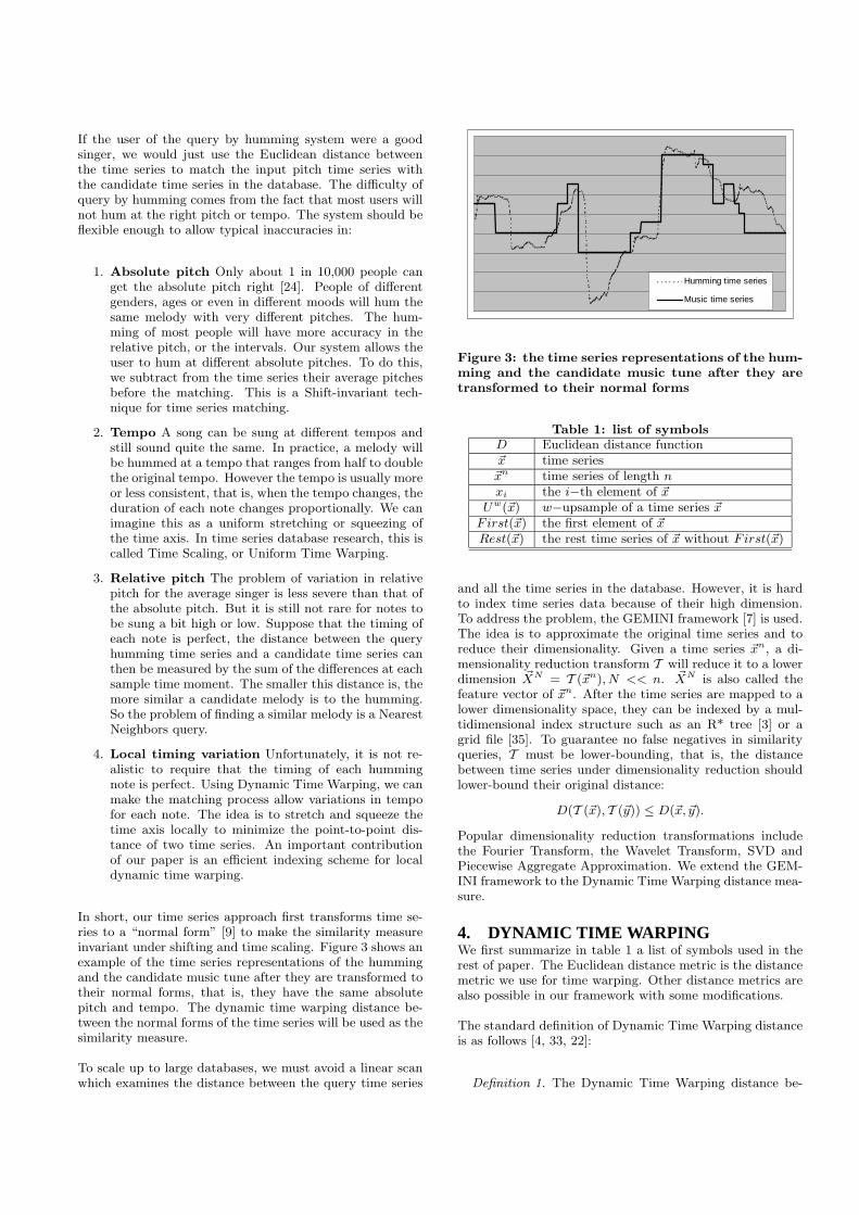
In short, our time series approach first transforms time se-ries to a “normal form” [9] to make the similarity measureinvariant under shifting and time scaling. Figure 3 shows anexample of the time series representations of the hummingand the candidate music tune after they are transformed totheir normal forms, that is, they have the same absolutepitch and tempo. The dynamic time warping distance be-tween the normal forms of the time series will be used as thesimilarity measure.
To scale up to large databases, we must avoid a linear scanwhich examines the distance between the query time series
Humming time series
Music time series
Figure 3: the time series representations of the hum-ming and the candidate music tune after they aretransformed to their normal forms
Table 1: list of symbolsD Euclidean distance function~x time series~xn time series of length n
xi the i−th element of ~xUw(~x) w−upsample of a time series ~x
First(~x) the first element of ~xRest(~x) the rest time series of ~x without First(~x)
and all the time series in the database. However, it is hardto index time series data because of their high dimension.To address the problem, the GEMINI framework [7] is used.The idea is to approximate the original time series and toreduce their dimensionality. Given a time series ~xn, a di-mensionality reduction transform T will reduce it to a lowerdimension ~XN = T (~xn), N << n. ~XN is also called thefeature vector of ~xn. After the time series are mapped to alower dimensionality space, they can be indexed by a mul-tidimensional index structure such as an R* tree [3] or agrid file [35]. To guarantee no false negatives in similarityqueries, T must be lower-bounding, that is, the distancebetween time series under dimensionality reduction shouldlower-bound their original distance:
D(T (~x), T (~y)) ≤ D(~x, ~y).
Popular dimensionality reduction transformations includethe Fourier Transform, the Wavelet Transform, SVD andPiecewise Aggregate Approximation. We extend the GEM-INI framework to the Dynamic Time Warping distance mea-sure.
4. DYNAMIC TIME WARPINGWe first summarize in table 1 a list of symbols used in therest of paper. The Euclidean distance metric is the distancemetric we use for time warping. Other distance metrics arealso possible in our framework with some modifications.
The standard definition of Dynamic Time Warping distanceis as follows [4, 33, 22]:
Definition 1. The Dynamic Time Warping distance be-

tween two time series ~x,~y is
D2DTW (~x, ~y) = D
2(First(~x), F irst(~y))
+min
D2DTW (~x,Rest(~y))
D2DTW (Rest(~x), ~y)
D2DTW (Rest(~x), Rest(~y))
The process of computing the DTW distance can be visual-ized as a string matching style dynamic program (figure 4).We construct a n×m matrix to align time series ~xn and ~ym.The cell (i, j) corresponds to the alignment of the elementxi with yj . A warping path, P , from cell (1, 1) to (n,m)corresponds to a particular alignment, element by element,between ~xn and ~ym:
P = p1, p2, ..., pL = (px1 , p
y1), (p
x2 , p
y2), ..., (p
xL, p
yL)
max(n,m) ≤ L ≤ n+m− 1
pxt , p
yt , t = 1, 2, ..., L are the position numbers of ~x
n and ~ym
respectively in the alignment. The distance between ~xn and~ym on the warping path P is the distance between xpx
tand
ypyt, t = 1, 2, ..., L. The constraints on the path P are:
• P must be monotonic :pxt −px
t−1 ≥ 0 and pyt −p
yt−1 ≥ 0
• P must be continuous :pxt −px
t−1 ≤ 1 and pyt −p
yt−1 ≤ 1
The number of possible warping paths grows exponentiallywith the length of the time series. The distance that is mini-mized over all paths is the Dynamic Time Warping distance.It can be computed using Dynamic Programming in O(mn)time [4].
4.1 Uniform time warpingUniform Time Warping (UTW) is a special case of DTW.The constraint imposed by UTW is that the warping pathmust be diagonal.
Definition 2. The Uniform Time Warping distance be-tween two time series ~xn, ~ym is
D2UTW (~x
n, ~y
m) =
∑mni=1(xdi/me − ydi/ne)
2
mn
For simplicity of notation, we stretch both time axis of~xn, ~ym to be mn. It is clear that if their greatest commondivisor, GCD(m,n) > 1, the time axis can be stretched toonly their least common multiple, LCM(n,m).
Using the concept of upsampling, the definition of UniformTime Warping can be simplified.
Definition 3. The w−upsampling of a time series ~xn is
Uw(~xn) = ~z
nw
zi = xdi/we, i = 1, 2, ..., nw
Intuitively, w−upsampling repeats each value in a time se-ries w times. The following lemma makes it possible toreduce the UTW distance to Euclidean distance.
Lemma 1.
D2UTW (~x
n, ~y
m) =D2(Um(~xn), Un(~ym)
)
mn
Uniform Time Warping is a generalization of Time Scaling.In time scaling, the length of one time series must be amultiple of the length of the other, while there is no sucha restriction for UTW. Using UTW, we can compute thedistance between time series of different lengths. The UTWnormal form of a time series ~xn is Uw(~xn), where nw is apredefined large number. It is not hard to adjust existingdimensionality reduction techniques to compute the UTWnormal form of a time series.
4.2 Local dynamic time warpingThe constraint imposed by UTW is too rigid, but it can berelaxed by Local Dynamic Time Warping (LDTW). Intu-itively, humans will match two time series of different lengthsas follows. First, the two time series are globally stretchedto the same length. They are then compared locally pointby point, with some warping within a small neighborhood inthe time axis. Such a two-step transform can emulate tradi-tional Dynamic Time Warping while avoiding some unintu-itive results as well as speeding it up. Here is the definitionof Local Dynamic Time Warping.
Definition 4. The k−Local Dynamic Time Warping dis-tance between two time series ~x,~y is
D2LDTW (k)(~x, ~y) = D
2constraint(k)(First(~x), F irst(~y))
+min
D2LDTW (k)(~x,Rest(~y))
D2LDTW (k)(Rest(~x), ~y)
D2LDTW (k)(Rest(~x), Rest(~y))
D2constraint(k)(xi, yj) =
{D2(xi, yj) if |i− j| ≤ k
∞ if |i− j| > k
Figure 4 shows a warping path for DLDTW (2)in a time warp-ing grid. The possible paths are constrained to be withinthe shadow, which is a beam of width 5(= 2∗2+1) along thediagonal path. The warping width is defined as δ = 2k+1
n.
Such a constraint is also known as a Sakoe-Chiba Band.Other similar constraints are also discussed in [13]. It can beshown that the complexity of computing k−Local DynamicTime Warping Distance is O(kn) using dynamic program-ming.
Note that in the work [13], the definition of the DTW isactually LDTW. By combining UTW and LDTW together,we define a more general DTW distance:
Definition 5. The Dynamic Time Warping distance be-tween two time series is the LDTW distance between theirUTW normal forms.

0 1 2
0
1
2
3
4
5
6
7
8
9
10
11
3 4 5 6 7 8 9 10 11
j
i
Figure 4: An example warping path with local con-straint
In other words, it is the LDTW distance between two timeseries after they are both upsampled to be of the samelength. In a slight abuse of notation, we will not distinguishLDTW and DTW in the remaining of the paper, and weassume the distance of LDTW is computed after the UTWtransform had been performed on the time series.
4.3 Lower-bounding technique and indexingscheme
The Local Dynamic Time Warping distance makes it pos-sible to lower-bound the distance locally. Because such alocal lower-bound is tighter than the global lower-boundingfor DTW [33], it produces fewer false positives.
To simplify our notation, we will first introduce the conceptof envelope for time series.
Definition 6. The k−Envelope of a time series ~x = xi, i =1, ..., n is
Envk(~x) = (EnvLk (~x);Env
Uk (~x)).
EnvLk (~x) and EnvU
k (~x) are the upper and lower envelope of~x respectively:
EnvLk (~x) = x
Li , i = 1, ..., n;x
Li = min−k≤j≤k(xi+j)
EnvUk (~x) = x
Ui , i = 1, ..., n;xU
i = max−k≤j≤k(xi+j)
~e = ~eL;~eU denotes the envelope of a time series. The dis-tance between a time series and an envelope is defined nat-urally as follows.
Definition 7. The distance between a time series ~x andan envelope ~e is
D(~x,~e) = min~z∈~e
D(~x, ~z)
We use ~zn ∈ ~e to denote that eLi ≤ zi ≤ eU
i , i = 1, 2, ..., n.So the value at each point can be any one in the range.
Keogh [13] proved that the distance between a time seriesand the envelope of another time series lower-bounds thetrue DTW distance.
Lemma 2. [13]
D(~xn, Envk(~y
n)) ≤ DDTW (k)(~xn, ~y
n)
To index the time series in the GEMINI framework, oneneeds to perform dimensionality reduction transform on thetime series and its envelope. Piecewise Aggregate Approx-imation (PAA) is used in [13]. The PAA of the time series
~xn is ~XN , N << n, where
Xi =N
n
nN
i∑
j= nN
(i−1)+1
xj , i = 1, 2, ..., N.
That is, the n dimensional time series ~xn is reduced todimension N by taking averages in N consecutive equalsized “frames”. The PAA reduction of the envelopes usingKeogh’s method is as follows. Let (~LN ; ~UN ) be the PAA
reduction of an envelope (~ln; ~un),
Li = min(l nN
(i−1)+1, ..., l nN
i),
Ui = max(u nN
(i−1)+1, ..., u nN
i), i = 1, 2, ..., N.
The PAA of an envelope is just the piecewise constant func-tion, which bounds but does not intersect the envelope.
We introduce a new PAA reduction as follows.
Li =N
n
nN
i∑
j= nN
(i−1)+1
lj , Ui =N
n
nN
i∑
j= nN
(i−1)+1
uj .
i = 1, 2, ..., N
In our method, ~U and ~L are also piecewise constant func-tions, but each piece is the average of the upper or lowerenvelope during that time period. Figure 5-a shows a timeseries, its bounding envelope and the PAA reduction of theenvelope using Keogh’s method. Figure 5-b shows the sametime series, its bounding envelops and the PAA reductionof the envelope using our method. We can see clearly thatthe bounds in figure 5-b are tighter than that in figure 5-aand it is straightforward to prove that this is always the casefor any time series. We will show that our bounds can stillguarantee to lower-bound the real DTW distance.
Before we prove that our PAA transform can provide alower-bound for DTW, we will first discuss general dimen-sionality reduction transforms on envelopes for indexing timeseries under the DTW distance. This is a principle contri-bution of the paper. We define the container property of adimensionality reduction transform for an envelope as fol-lows.
Definition 8. We say a transformation T for an envelope~e is “container-invariant” if
∀~xnif ~x
n ∈ ~e then T (~xn) ∈ T (~e)

Original time seriesUpper envelopeLower envelopeU_KeoghL_Keogh
Original time seriesUpper envelopeLower envelopeU_newL_new
Figure 5: The PAA for the envelope of a timeseries using (a)Keogh’s method(top) and (b)Ourmethod(bottom).
Just as a transform of time series that is lower-bounding canguarantee no false negatives for Euclidean distance, a trans-form of envelopes that is container-invariant can guaranteeno false negatives for DTW distance.
Theorem 1. If a transformation T is container-invariantand lower-bounding then
D(T (~x), T (Envk(~y))) ≤ DDTW (k)(~x, ~y)
Proof. T is container-invariant,
∴ ∀~znif ~z
n ∈ ~e then T (~zn) ∈ T (~e)
∴ {~z|~z ∈ Envk(~y)} ⊆ {~z|T (~z) ∈ T (Envk(~y))}
∴ min{~z|T (~z)∈T (Envk(~y))}
D(~x, ~z) ≤ min{~z|~z∈Envk(~y)}
D(~x, ~z)
T is lower-bounding,
∴ D(T (~x), T (~z)) ≤ D(~x, ~z)
∴ min{~z|T (~z)∈T (Envk(~y))}
D(T (~x), T (~z)) ≤ min{~z|T (~z)∈T (Envk(~y))}
D(~x, ~z)
∴ min{~z|T (~z)∈T (Envk(~y))}
D(T (~z), T (~z)) ≤ min{~z|~z∈Envk(~y)}
D(~x, ~z)
By the definition of distance between time series and enve-lope,
D(T (~x), T (Envk(~y))) ≤ D(~x,Envk(~y))
From lemma 2,
D(T (~x), T (Envk(~y))) ≤ DDTW (k)D(~x, ~y)
Using the concept of container-invariant, we can design thetransform for the envelope based on PAA, DWT, SVD andDFT. All these dimensionality reduction transforms are lin-ear transforms1, that is,
~XN = T (~xn), Xj =
n∑
i=1
aijxi, j = 1, 2, ..., N.
We can extend such linear transforms for time series totransforms for time series envelopes, and at the same timeguarantee they are container-invariant.
Lemma 3. Let transform T be a linear transform, ~XN =T (~xn), Xj =
∑ni=1 aijxi, j = 1, 2, ..., N , and the transform
T on envelope ~e is as follows,
E = ( ~EL, ~E
U ) = T (~eL, ~e
U )
EUj =
n∑
i=1
(aijeUi τ(aij) + aije
Li (1− τ(aij)))
ELj =
n∑
i=1
(aijeLi τ(aij) + aije
Ui (1− τ(aij)))
j = 1, 2, ..., N
where τ is the sign function:
τ(x) =
{1 x ≥ 00 x < 0
Then transform T is container-invariant.
Proof.
∀~xnif ~x
n ∈ ~e then eLi ≤ xi ≤ e
Ui , i = 1, 2, ..., n
Therefore ELi ≤ Xj ≤ E
Ui , j = 1, 2, ..., N
∴ T (~xn) ∈ T (~e)
A transform of an envelope is still an envelope, which we callthe envelope in the feature space. In the special case whenthe envelope equals the time series, the transform of the en-velope becomes the transform of the time series. BecausePAA is a linear transform, and our proposed PAA trans-form for envelopes is deduced from the lemma above, it iscontainer-invariant. PAA also has the nice property thatall the coefficients of linear transformation for PAA, unlikeDFT and SVD, are positive. In this case, the upper enve-lope in feature space is just the PAA transform of the upperenvelope, so is the lower envelope. For other transform likeDFT and SVD, the upper envelope in feature space is thetransform of the combination of the upper and the lowerenvelope. So the envelopes in the PAA feature space aretighter then those for DFT and SVD in general. Our exper-iments also confirm this.
1 DFT is a linear transform because the real and image partof a DFT coefficient are still a linear combination of theoriginal time series.

Now we are ready to describe the strategy for time seriesdatabase query with DTW. An ε-range similarity query ina time series database is to find all the time series whosedistances with the query are less than ε. It includes thefollowing step.
1. For each time series ~xn in the database, compute itsfeature vector ~XN .
2. Build an N -dimensional index structure on ~XN .
3. For a time series query ~qn, compute its envelope ~en
and ~EN = T (~en).
4. Make an ε-range query of ~EN on the index structure,and return a set of time series S.
5. Filter out the false positives in S using their true DTWdistances with ~qn. We can guarantee no false negativesfrom theorem 1.
Similarly, a k-nearest neighbors query can be built on topof such a range query [17, 26]. For existing time seriesdatabases indexed by DFT, DWT, PAA, SVD, etc., we canadd Dynamic Time Warping support without rebuilding in-dices. This works because our framework allows all thelinear transforms and adding the DTW support requireschanges only to the time series query.
5. EXPERIMENTSOur experiments are divided into three parts. First we willrun experiments to evaluate the quality of our query byhumming system using the time series database approach.Comparisons with traditional contour based method will bemade. We will also test the efficiency of our DTW indexingscheme comparing to the state-of-the-art technique. Finallywe will test the scalability of our system.
5.1 Quality of the query by humming systemWe collected 50 of the most popular Beatles’s songs by man-ual entry. These songs are further segmented to 1000 shortmelodies. Each melody contains 15 to 30 notes. We askedpeople with different musical skills to hum for the system.
To evaluate the quality of the query by humming system,first we compared it with the note contour-based method.We will use the hum queries of better singers in this exper-iment, because for hum queries of poor quality it is hardfor even a human being to recognize the target song. Forthe note contour-based method, we need to transcribe theuser humming into discrete notes first. For lack of a re-liable note-segmentation algorithm, we used the best com-mercial software we could find, AKoff Music Composer[2], totranscribe notes. We also applied a standard algorithm [27]to transcribe the user hum query to a sequence of pitches,and used the silence information between pitches to segmentnotes. For the contour-based method, we report the betterresult based on these two note-segmentation processes. Forthe 20 pieces of hum queries by better singers, we searchedthe database to find their ranks using the contour-based ap-proach and the time series approach. The result is shown intable 2. We can see that our time series approach beats the
Table 2: The number of melodies correctly retrievedusing different approaches
Rank Time series Approach Contour Approach1 16 22-3 2 04-5 2 06-10 0 410- 0 14
Table 3: The number of melodies correctly retrievedby poor singers using different warping widths
Rank δ = 0.05 δ = 0.1 δ = 0.21 2 4 22-3 2 3 54-5 4 5 76-10 3 5 410- 9 3 2
contour approach clearly. We are not claiming that usingcontour information for music matching is bad. Howeveruntil a reliable note-segmentation algorithm is developed,such an approach is based on dubious input. If for exam-ple, the query input were by piano instead of human voiceso that each individual note is clearly separated, we wouldexpect the contour-base approach to have good quality too.
We tested our system with some hum queries of poor qual-ity, for example, by one of the authors. We define a melodyto be perfectly matched if it is the intended target melody ofthe hummer and its rank is 1. The number of melodies per-fectly matched is low. Still the result is quite encouraging.We noticed that the warping width can be adjusted to tunethe query results. It is hard for a poor hummer to keep theright duration for each note of the melody. Allowing largerwarping widths will give the hummers more flexibility inthe duration of the notes. For the 20 hum queries by poorsingers, we searched the database to find their ranks usingDTW with different warping width. The result is reportedin table 3. We can see that more queries return in the top 10matches when the warping width is increased from 0.05 to0.1. But this tendency disappears when the warping widthis increased to 0.2, because it is unlikely for a hummer tosing way off tempo. When the warping width is too large,some melodies that are very different will have a small DTWdistance too. A warping width of 1 for local DTW degener-ates to global DTW. Larger warping widths also slow downthe processing.
5.2 Experiments for indexing DTWHaving shown that our time series approach for query byhumming system has superior quality over the traditionalcontour approach, we will also demonstrate that it is veryefficient. Unlike [19], the performance of the time series ap-proach does not suffer from the extensive use of DTW. Thescalability of our system comes from our proposed techniquefor indexing DTW. We will compare our DTW indexingtechnique with the best existing DTW indexing method [13].There is an increasing awareness to use a benchmark ap-proach in time series database experiments to guard against

1 2 3 4 5 6 7 8 9 10 11 12 13 14 15 16 17 18 19 20 21 22 23 24
0
0.1
0.2
0.3
0.4
0.5
0.6
0.7
0.8
0.9
Tig
htne
ss o
f Low
er B
ound
Data set
Keogh_PAA
New _PAA
LB
Figure 6: The mean value of the tightness of lower bound, using LB, New PAA and Keogh PAA for differenttime series data sets. The data sets are 1.Sunspot; 2.Power; 3.Spot Exrates; 4.Shuttle; 5.Water; 6. Chaotic;7.Streamgen; 8.Ocean; 9.Tide; 10.CSTR; 11.Winding; 12.Dryer2; 13.Ph Data; 14.Power Plant; 15.Balleam;16.Standard &Poor; 17.Soil Temp; 18.Wool; 19.Infrasound; 20.EEG; 21.Koski EEG; 22.Buoy Sensor; 23.Burst;24.Randow walk
implementation bias and data bias. In the spirit of the work[15, 13], we took such an approach to conduct our experi-ments. To avoid data bias, we conducted our experimentson a wide range of time series datasets [12] that cover disci-plines including finance, medicine, industry, astronomy andmusic. We also measured the results in an implementationfree fashion to avoid bias in implementation.
We define the tightness of the lower bound for DTW distanceas follows.
T = Lower Bound of DTW distance based on reduced dimensionTrue DTW distance
T is in the range of [0,1]. Larger T gives a tighter bound.Note that the definition here is different from that in thework [13]. In [13], Keogh has shown convincingly that lower-bounding using the envelope is much tighter than globalbounding as reported in [33]. But such an envelope usesmuch more information than global lower-bounding. For atime series of size n, its envelope is represented by 2n val-ues. By contrast, the global lower-bounding technique canbe seen as using the minimum and maximum value of atime series as the envelope of a time series. So the globalbounding is represented by only 2 values. To test the effi-ciency of dimensionality reduction under DTW, we modifythe definition of T slightly, i.e., the lower-bound is basedon reduced dimension. We compared three methods: LB isthe lower-bound using the envelope (without dimensional-ity reduction and therefore without the possibility of index-ing); Keogh PAA is the lower-bound using PAA transforma-tion proposed by Keogh [13] and New PAA is our proposedPAA lower-bound. We chose each sequence to be of lengthn = 256 and a warping width to be 0.1. The dimension wasreduced from 256 to 4 using PAA. We selected 50 time seriesrandomly from each dataset and subtracted the mean fromeach time series. We computed the tightness of the lowerbound of the distances between each pair of the 50 time se-ries. The average tightness of lower bound for each datasetusing the three methods are reported in figure 6.
From the figure, we can see that the method LB has thebest T for each dataset. This is not a surprise, because themethod LB uses much more information than Keogh PAAand New PAA. We include it here as a sanity check. LB
0
0.1
0.2
0.3
0.4
0.5
0.6
0.7
0.8
0.9
1
0 0.01 0.02 0.03 0.04 0.05 0.06 0.07 0.08 0.09 0.1Warping Width
Tig
htne
ss o
f Lo
wer
Bou
nd
LBNew_PAAKeogh_PAASVDDFT
Figure 7: The mean value of the tightness of lowerbound changes with the warping widths, using LB,New PAA, Keogh PAA, SVD and DFT for the ran-dom walk time series data set.
will be used as a second filter after the indexing scheme,Keogh PAA or New PAA, returns a superset of answer. Us-ing the same number of values, New PAA is always betterthan Keogh PAA. That comes from the fact that the esti-mations of DTW using New PAA are always closer to thetrue DTW distance than the estimations using Keogh PAA.The tightness of lower bound of New PAA is approximately2 times that of Keogh PAA on average for all datasets.
One of the contributions of this paper is a framework allow-ing DTW indexing using different dimensionality reductionmethods in addition to PAA. The performance of compet-ing dimensionality reduction methods under the Euclideandistance measure is very data-dependent, none of them isknown to be the best in all cases. Allowing different di-mensionality reduction methods to be extended to the caseof the DTW distance measure will provide the users withmore flexibility in choosing the right method for a partic-ular application. We tested the tightness of lower boundsfor DTW indexing using dimensionality reduction methodsincluding PAA, DFT and SVD. For brevity, we will only re-port the results for the random walk data in figure 7, becausethe random walk data are the most studied dataset of timeseries indexing and are very homogeneous. We varied thewarping widths from 0 to 0.1. Each T value is the average

threshold=0.2
0
10
20
30
40
50
60
0.02 0.04 0.06 0.08 0.1 0.12 0.14 0.16 0.18 0.2
Warping Width
# of
Can
dida
tes
Keogh_PAA
New_PAA
threshold=0.8
0
20
40
60
80
100
120
0.02 0.04 0.06 0.08 0.1 0.12 0.14 0.16 0.18 0.2
Warping Width
# of
Can
dida
tes
Keogh_PAA
New_PAA
Figure 8: The number of candidates to be retrievedwith different query thresholds for the Beatles’smelody database
of 500 experiments. Again LB is always the tightest lower-bound because no dimensionality reduction is performed. Inthe case of 0 warping width, the DTW distance is the sameas the Euclidean distance. Since SVD is the optimal di-mensionality reduction method for Euclidean distance, thelower-bound using SVD is tighter than any other dimen-sionality reduction methods. The performance of DFT andPAA for the Euclidean distance measure is similar, whichconfirms other research [30, 14]. For all the warping widths,New PAA is always better that Keogh PAA as we wouldexpect. New PAA also beats DFT and SVD as the warpingwidths increase. The reason is that all the linear transfor-mation coefficients for PAA are positive, as we mentionedbefore.
5.3 Scalability testingThe tightness of the lower bound is a good indicator of theperformance of a DTW indexing scheme. A tighter lower-bound means that fewer candidates need to be retrieved forfurther examination in a particular query. That will increasethe precision of retrieval at no cost to recall. Higher preci-sion of retrieval implies lower CPU cost and IO cost at thesame time, because we need to access fewer pages to retrievecandidate time series and to perform fewer exact DynamicTime Warping computations. We will use the number ofcandidates retrieved and the number of page accesses as theimplementation-bias free measures for the CPU and IO cost.
First we conducted experiments on our small music databaseof the Beatles’s songs. Figure 8 shows the average numbercandidates to be retrieved for queries with different selectiv-ity. The range queries have range nε, n is the length of thetime series and the thresholds ε take the values of 0.2 and0.8. From the figure, we can see that as the warping widthsget larger, the number of candidates retrieved increases, be-cause the lower-bounds get looser for larger warping widths.Our approach (New PAA) is up to 10 times better thanKeogh PAA.
To test the scalability of our system, we need to use largerdatasets. The first database we tested is a music database.We extracted notes from the melody channel of MIDI fileswe collected from the Internet and transformed them to ourtime series representation. There are 35, 000 time series inthe database. The second database contains 50, 000 randomwalk data time series. Each time series has a length of 128and is indexed by its 8 reduced dimensions using an R* tree[3] implemented in LibGist [10]. Each result we report isaveraged over 500 experiments. Figure 9 shows the perfor-mance comparisons for the music database. We can see thatthe number of page accesses is proportional to the numberof candidates retrieved for all the methods and thresholds.In a Pentium 4 PC, NEW PAA took from 1 second for thesmallest warping width to 10 seconds for the largest warpingwidth. As the warping width increases, the number of candi-dates retrieved increases significantly using the Keogh PAAmethod while it increases less for New PAA. This is also truefor other time series datasets. Figure 10 shows the perfor-mance comparisons for the random walk database. Similarperformance advantages of our method hold for the randomwalk data too.
6. CONCLUSIONSWe present an improved scheme for indexing time seriesdatabases using Dynamic Time Warping. Our improvementbuilds on the dimensionality reduction transform of timeseries envelopes. We give a general approach to adaptingexisting time series indexing schemes for the Euclidean dis-tance measure to the DTW distance measure. We prove thatsuch an indexing scheme guarantees no false negatives giventhat the dimensionality reduction on envelope is container-invariant. Using this approach, our PAA transform for DTWis consistently better than the previous reported PAA trans-form. Extensive experiments showed that the improvementis by a factor between 3 and 10.
Based on the time warping indexes, we show that the timeseries database approach for query by humming gives highprecision and is fast and scalable. We have also implementeda query by humming system. Preliminary testing of the sys-tem on real people (OK, our friends) gave good performanceand high satisfaction. Some even improved their singing asa result. The system is not yet mature. We are still workingon expanding our melody database and adapting the sys-tem to different hummers. However, the system’s potentialapplications to entertainment and education are fortissimo.
7. ACKNOWLEDGMENTSWe are grateful to Prof. Eamonn Keogh for providing theUCR time series data mining archive. We thank DominicMazzoni for providing the transcription software. We thankHsiao-Lan Hsu for her input of the Beatles’s songs. Andmany thanks to our friends for testing the system by hum-ming.
8. REFERENCES[1] R. Agrawal, C. Faloutsos, and A. N. Swami. EfficientSimilarity Search In Sequence Databases. InD. Lomet, editor, Proceedings of the 4th InternationalConference of Foundations of Data Organization andAlgorithms (FODO), pages 69–84, Chicago, Illinois,1993. Springer Verlag.

threshold=0.2
0
50
100
150
200
250
300
350
400
0.02 0.04 0.06 0.08 0.1 0.12 0.14 0.16 0.18 0.2
Warping Width
# of
Can
dida
tes
Keogh_PAA
New_PAA
threshold=0.8
0
100
200
300
400
500
600
0.02 0.04 0.06 0.08 0.1 0.12 0.14 0.16 0.18 0.2
Warping Width
# of
Can
dida
tes
Keogh_PAA
New_PAA
threshold=0.2
0
10
20
30
40
50
60
0.02 0.04 0.06 0.08 0.1 0.12 0.14 0.16 0.18 0.2
Warping Width
# of
Pag
e A
cces
ses
Keogh_PAA
New_PAA
threshold=0.8
0
10
20
30
40
50
60
70
80
0.02 0.04 0.06 0.08 0.1 0.12 0.14 0.16 0.18 0.2
Warping Width
# of
Pag
e A
cces
ses
Keogh_PAA
New_PAA
Figure 9: Performance comparisons with different query thresholds for a large music database
threshold=0.2
0
10
20
30
40
50
60
70
80
90
100
0.02 0.04 0.06 0.08 0.1 0.12 0.14 0.16 0.18 0.2
Warping Width
# of
Can
dida
tes
Keogh_PAA
New_PAA
threshold=0.8
0
50
100
150
200
250
300
350
400
450
0.02 0.04 0.06 0.08 0.1 0.12 0.14 0.16 0.18 0.2
Warping Width
# of
Can
dida
tes
Keogh_PAA
New_PAA
threshold=0.2
0
5
10
15
20
25
30
0.02 0.04 0.06 0.08 0.1 0.12 0.14 0.16 0.18 0.2
Warping Width
# of
Pag
e A
cces
ses
Keogh_PAA
New_PAA
threshold=0.8
0
10
20
30
40
50
60
0.02 0.04 0.06 0.08 0.1 0.12 0.14 0.16 0.18 0.2
Warping Width
# of
Pag
e A
cces
ses
Keogh_PAA
New_PAA
Figure 10: Performance comparisons with different query thresholds for a large random walk database
[2] AKoff Sound Labs. Akoff music composer version2.0,http://www.akoff.com/music-composer.html, 2000.
[3] N. Beckmann, H.-P. Kriegel, R. Schneider, andB. Seeger. The r*-tree: An efficient and robust accessmethod for points and rectangles. In Proceedings ofthe 1990 ACM SIGMOD International Conference onManagement of Data, Atlantic City, NJ, May 23-25,1990, pages 322–331, 1990.
[4] D. Berndt and J. Clifford. Using dynamic timewarping to find patterns in time series. In Advances inKnowledge Discovery and Data Mining, pages229–248. AAAI/MIT, 1994.
[5] S. G. Blackburn and D. C. DeRoure. A tool forcontent based navigation of music. In ACMMultimedia 98, pages 361–368, 1998.
[6] K.-P. Chan and A. W.-C. Fu. Efficient time seriesmatching by wavelets. In Proceedings of the 15th
International Conference on Data Engineering,Sydney, Australia, pages 126–133, 1999.
[7] C. Faloutsos, M. Ranganathan, and Y. Manolopoulos.Fast subsequence matching in time-series databases.In Proc. ACM SIGMOD International Conf. onManagement of Data, pages 419–429, 1994.
[8] A. Ghias, J. Logan, D. Chamberlin, and B. C. Smith.Query by humming: Musical information retrieval inan audio database. In ACM Multimedia 1995, pages231–236, 1995.
[9] D. Q. Goldin and P. C. Kanellakis. On similarityqueries for time-series data: Constraint specificationand implementation. In Proceedings of the 1stInternational Conference on Principles and Practiceof Constraint Programming (CP’95), 1995.
[10] J. M. Hellerstein, J. F. Naughton, and A. Pfeffer.Generalized search trees for database systems. In

U. Dayal, P. M. D. Gray, and S. Nishio, editors, Proc.21st Int. Conf. Very Large Data Bases, VLDB, pages562–573. Morgan Kaufmann, 11–15 1995.
[11] J.-S. R. Jang and H.-R. Lee. Hierarchical filteringmethod for content-based music retrieval via acousticinput. In Proceedings of the ninth ACM internationalconference on Multimedia, pages 401–410. ACM Press,2001.
[12] E. Keogh and T. Folias. The UCR Time Series DataMining Archive[http://www.cs.ucr.edu/ ea-monn/tsdma/index.html],Riverside CA. University ofCalifornia - Computer Science and EngineeringDepartment, 2002.
[13] E. J. Keogh. Exact indexing of dynamic time warping.In VLDB 2002,Proceedings of 28th InternationalConference on Very Large Data Bases, August 20-23,2002, Hong Kong, China, pages 406–417, 2002.
[14] E. J. Keogh, K. Chakrabarti, S. Mehrotra, and M. J.Pazzani. Locally adaptive dimensionality reduction forindexing large time series databases. In Proc. ACMSIGMOD International Conf. on Management ofData, 2001.
[15] E. J. Keogh and S. Kasetty. On the need for timeseries data mining benchmarks: A survey andempirical demonstration. In the 8th ACM SIGKDDInternational Conference on Knowledge Discovery andData Mining,July 23 - 26, 2002. Edmonton, Alberta,Canada, pages 102–111, 2002.
[16] F. Korn, H. V. Jagadish, and C. Faloutsos. Efficientlysupporting ad hoc queries in large datasets of timesequences. In SIGMOD 1997, Proceedings ACMSIGMOD International Conference on Management ofData, May 13-15, 1997, Tucson, Arizona, USA, pages289–300, 1997.
[17] F. Korn, N. Sidiropoulos, C. Faloutsos, E. Siegel, andZ. Protopapas. Fast nearest neighbor search inmedical image databases. In VLDB’96, Proceedings of22th International Conference on Very Large DataBases, September 3-6, 1996, Mumbai (Bombay), India,pages 215–226, 1996.
[18] N. Kosugi, Y. Nishihara, T. Sakata, M. Yamamuro,and K. Kushima. A practical query-by-hummingsystem for a large music database. In ACMMultimedia 2000, pages 333–342, 2000.
[19] D. Mazzoni and R. B. Dannenberg. Melody matchingdirectly from audio. In 2nd Annual InternationalSymposium on Music InformationRetrieval,Bloomington, Indiana, USA, 2001.
[20] R. J. McNab, L. A. Smith, D. Bainbridge, and I. H.Witten. The new zealand digital library melody index.In D-Lib Magazine, 1997.
[21] Y.-S. Moon, K.-Y. Whang, and W.-S. Han.Generalmatch: A subsequence matching method intime-series databases based on generalized windows.In SIGMOD 2002,Madison,Wisconsin, USA, 3-6 June2002., 2002.
[22] S. Park, W. W. Chu, J. Yoon, and C. Hsu. Fastretrieval of similar sub-sequences under time warping.In ICDE, pages 23–32, 2000.
[23] I. Popivanov and R. J. Miller. Similarity search overtime series data using wavelets. In ICDE, 2002.
[24] J. Profita and T.G.Bidder. Perfect pitch. In AmericanJournal of Medical Genetics, pages 763–771, 1988.
[25] D. Rafiei and A. Mendelzon. Similarity-based queriesfor time series data. In Proc. ACM SIGMODInternational Conf. on Management of Data, pages13–25, 1997.
[26] T. Seidl and H.-P. Kriegel. Optimal multi-stepk-nearest neighbor search. In L. M. Haas andA. Tiwary, editors, SIGMOD 1998, Proceedings ACMSIGMOD International Conference on Management ofData, June 2-4, 1998, Seattle, Washington, USA,pages 154–165, 1998.
[27] T. Tolonen and M. Karjalainen. A computationallyefficient multi-pitch analysis model. IEEETransactions on Speech and Audio Processing, 2000.
[28] A. Uitdenbgerd and J. Zobel. Manipulation of musicfor melody matching. In ACM Multimedia 98, pages235–240, 1998.
[29] A. Uitdenbgerd and J. Zobel. Melodic matchingtechniques for large music databases. In ACMMultimedia 99, pages 57–66, 1999.
[30] Y.-L. Wu, D. Agrawal, and A. E. Abbadi. Acomparison of dft and dwt based similarity search intime-series databases. In Proceedings of the 9 thInternational Conference on Information andKnowledge Management, 2000.
[31] C. Yang. Efficient acoustic index for music retrievalwith various degrees of similarity. In ACM Multimedia2002, December 1-6, 2002,French Riviera, 2002.
[32] B.-K. Yi and C. Faloutsos. Fast time sequenceindexing for arbitrary lp norms. In VLDB 2000,Proceedings of 26th International Conference on VeryLarge Data Bases, September 10-14, 2000, Cairo,Egypt, pages 385–394. Morgan Kaufmann, 2000.
[33] B.-K. Yi, H. V. Jagadish, and C. Faloutsos. Efficientretrieval of similar time sequences under time warping.In ICDE, pages 201–208, 1998.
[34] Y. Zhu, M. S. Kankanhalli, and C. Xu. Pitch trackingand melody slope matching for song retrieval. InAdvances in Multimedia Information Processing -PCM 2001, Second IEEE Pacific Rim Conference onMultimedia, Bejing, China, October 24-26, 2001.
[35] Y. Zhu and D. Shasha. Statstream: Statisticalmonitoring of thousands of data streams in real time.In VLDB 2002,Proceedings of 28th InternationalConference on Very Large Data Bases, August 20-23,2002, Hong Kong, China, pages 358–369, 2002.