watersupply (2).ppt

7/27/2019 WaterSupply (2).ppt

http://slidepdf.com/reader/full/watersupply-2ppt 1/15

Water Supply Study

Present and Planned Water Supply

• Operational (2001) spring water bottling plant,

with groundwater extraction rates

approximating 125 gpm.• Planned groundwater extraction of up to 400

gpm.

• Concerns about impacts to nearby water

bodies.



Critical Prediction

Calcu late changes in Sur face-

Water Flow s, Wetland and Lake Levels from Constant

Produc t ion of 400 gpm



0ft 10000ft 20000ft

Regional Model Design

Study Area

Selected CodeMODFLOW2000

Model Summary4 layers

Conductivity zones derived from

regional/local geologic studies

Variable recharge derived from

published regression analysis



Local Model Area

Impoundment

Stream

Pumping

Center

Spring

Outfall

Groundwater

Flow



Shortcomings in Problem

FormulationModeling Tool – Use of River Package

• Inability to realistically represent changes

in streams, wetlands, and lakes.

• Inability to explicitly represent the

impoundment-overflow



Stream

Impoundment Culvert

Discharge

Stream



Revised Problem Formulation

• Digitized stream intersections and topo maps to assign

MODFLOW Drain/River - revised during calibration.

• Impoundment and nearby lakes represented with Lake

Package (Merritt and Konikow, 2000); outflow fromimpoundment explicitly modeled.

• Four wetlands with standing water modeled with Lake

Package to explicitly simulate wetland water levels.

• Stream simulated using MODFLOW Drain Package

plus Impoundment outflow.

• Regional river comprises down gradient drainage

center.



Model Calibration

Calibration Strategy

• Steady-state calibration to water levels in 48 wells,

baseflow in five creeks, and lake levels in five lakes.

• Transient calibration to drawdowns from long-term (72hour) pumping test - one dozen wells with time-series

drawdown data

• Prior information used to establish total transmissivity

as ‘soft’ information during steady-state calibration

• Approx. 40 parameters – step-wise reduction using

tied/untied parameters as calibration progressed

• PEST used in parallel across four 1.8GHz processors



PEST Pre-Post Processing

Advantages over GUI or ‘prompt’ Execution

• Ability to assess progress with every run

• Ability to re-parameterize (tie, hold, transform, scale,

prior, regularize) model without ‘rebuild’

• Ability to alter run type with one (or two) quick Control

File modifications – Forward run, Estimation,

Regularization, and Prediction

goto 20



goto 20

Open(1,file='MICHIGAN_No_Reaches.riv')

Open(2,file='Michigan_reaches.riv')

c MODFLOW 2000 headers

Read(1,*)

Read(1,*)

Read(1,*) nriv,idum

Write(2,'(2I10)') nriv,idum

Read(1,*) nriv

Write(2,*) nriv

c Lay, Row, Col

Do n=1,nrivRead(1,*) k,i,j,stage,cond,rbot

Write(2,2) k,i,j,stage,cond*10,rbot,iriv_rch(j,i)

End do

Close(1)

Close(2)

Open(1,file='MICHIGAN_No_Reaches.drn')

Open(2,file='Michigan_reaches.drn')

c MODFLOW 2000 headers

Read(1,*)

Read(1,*)

Read(1,*) nriv,idum

Write(2,'(2I10)') nriv,idum

Read(1,*) nriv

Write(2,*) nriv

Do n=1,nriv

c Lay, Row, Col

Read(1,*) k,i,j,rbot,cond

Write(2,3) k,i,j,rbot,cond,idrn_rch(j,i)

End do

Close(1)

Close(2)

20 Continue

c=======================================================================

c FORMAT STATEMENTS

c=======================================================================

1 Format(4I11,F21.0)

2 Format(3I10,F10.3,E10.3,F10.3,I10)

3 Format(3I10,F10.3,E10.3,I10)

c=======================================================================

c END OF PROGRAM

c=======================================================================

STOP 'Normal Exit'

END

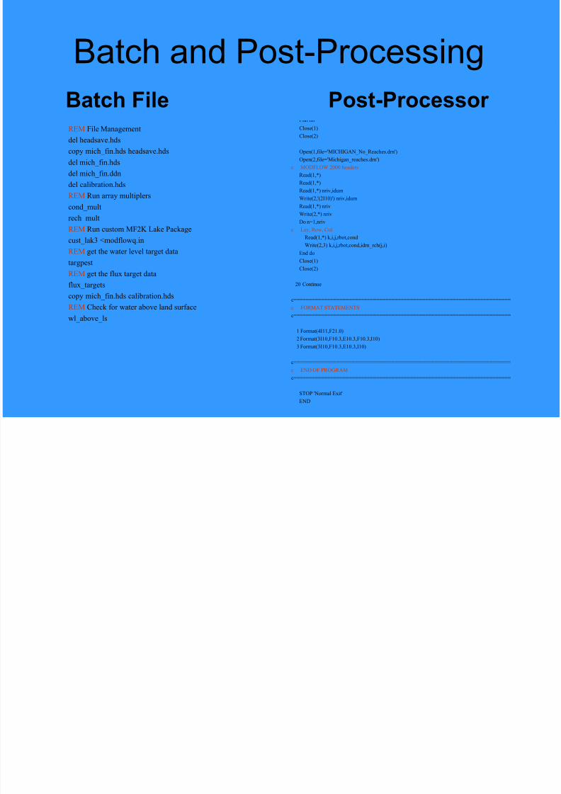
Batch File

Batch and Post-Processing

Post-Processor REM File Management

del headsave.hds

copy mich_fin.hds headsave.hds

del mich_fin.hds

del mich_fin.ddn

del calibration.hds

REM Run array multiplerscond_mult

rech_mult

REM Run custom MF2K Lake Package

cust_lak3 <modflowq.in

REM get the water level target data

targpest

REM get the flux target data

flux_targets

copy mich_fin.hds calibration.hds

REM Check for water above land surface

wl_above_ls



Calibration Results – SS

Baseflows Water Levels

0.E+00

1.E+06

2.E+06

3.E+06

4.E+06

0.E+00 1.E+06 2.E+06 3.E+06 4.E+06

940.0

960.0

980.0

1000.0

1020.0

1040.0

9.4E+02 9.6E+02 9.8E+02 1.0E+03 1.0E+03 1.0E+03

WL Sum of Squares (PHI) = ~ 115 ft2

Count = 48 wells

Mean Residual = - 0.2 ft

Mean Absolute Residual = 1.1 ft

StDev of the residuals = 1.5 ft

Range = 63 ftStDev/Range = ~ 2.25%



Calibration Results – Transient

Drawdowns



Predictive Analysis

Problem Formulation and Execution

• Reformulate the PEST calibration control file to

estimate the max and min baseflow depletions in

stream, while maintaining calibration – i.e. establishthe range of uncertainty

• Typically the increment added to the calibration

objective function (Fmin + d) is about 5% of Fmin.

For our analysis, this was raised by 50%



Predictive Analysis

Present and Planned Water Supply

• With total planned groundwater extraction of 400 gpm.

-Predicted stream depletion at regional river: 400 gpm

-Depletion of interest stream: small but measurable*

-Changes in wetland water levels: small but measurable*

The calculated upper- and lower-bound estimates of the change in flow

at the stream are on the order of five percent (above or below) of the

‘most likely’ estimated change.

*This is consistent with the observation that wetland water levels, and the areal extent of wetlands based on aerial photographs were not significantly affected by the construction of

the impoundment .



Salient Point(s)

• Problem formulation is key to the ‘integrity’ of the

predictive analysis – the selected code must be

designed to simulate the type of prediction of

interest.

• The fairly tight bounds on the prediction may also

arise from the ability of models to predict changes

far better than absolute numbers.

watersupply (2).ppt

Documents