1

Wavelet-Based Combined Signal Filtering andPrediction

Olivier Renaud, Jean-Luc Starck, and Fionn Murtagh

Abstract— We survey a number of applications of thewavelet transform in time series prediction. We showhow multiresolution prediction can capture short-rangeand long-term dependencies with only a few parametersto be estimated. We then develop a new multiresolutionmethodology for combined noise filtering and prediction,based on an approach which is similar to the Kalmanfilter. Based on considerable experimental assessment, wedemonstrate the powerfulness of this methodology.

Index Terms— Wavelet transform, filtering, forecast-ing, resolution, scale, autoregression, time series, model,Kalman filter.

I. I NTRODUCTION

There has been abundant interest in waveletmethods for noise removal in 1D signals. In manyhundreds of papers published in journals throughoutthe scientific and engineering disciplines, a widerange of wavelet-based tools and ideas have beenproposed and studied. Initial efforts included verysimple ideas like thresholding of the orthogonalwavelet coefficients of the noisy data, followed byreconstruction. More recently, tree-based waveletdenoising methods were developed in the contextof image denoising, which exploit tree structuresof wavelet coefficients and parent-child correlations,which are present in wavelet coefficients. Also,many investigators have experimented with vari-ations on the basic schemes – modifications ofthresholding functions, level-dependent threshold-ing, block thresholding, adaptive choice of thresh-old, Bayesian conditional expectation nonlinearities,and so on. In parallel, several approaches have beenproposed for time-series filtering and prediction bythe wavelet transform, based on a neural network

O. Renaud is with Methodology and Data Analysis, Section ofPsychology, University of Geneva, 1211 Geneva 4, Switzerland. J.-L.Starck is with DAPNIA/SEDI-SAP, Service d’Astrophysique, CEA-Saclay, 91191 Gif sur Yvette, France. F. Murtagh is with the Depart-ment of Computer Science, Royal Holloway, University of London,Egham, Surrey TW20 0EX, England. Contact for correspondence,F.Murtagh, fmurtagh@acm.org

[24], [3], [14], Kalman filtering [6], [13], or an AR(autoregressive) model [19]. In Zheng et al. [24] andSoltani et al. [19], the undecimated Haar transformwas used. This choice of the Haar transform wasmotivated by the fact that the wavelet coefficientsare calculated only from data obtained previouslyin time, and the choice of an undecimated wavelettransform avoids aliasing problems. See also Daoudiet al. [7], which relates the wavelet transform to amultiscale autoregressive type of transform.

In this paper, we propose a new combined pre-diction and filtering method, which can be seen asa bridge between the wavelet denoising techniquesand the wavelet predictive methods. Section II in-troduces the wavelet transform for time series, andsection III describes the Multiscale AutoregressiveModel (MAR), that is based on the above transform.It can be used either merely for prediction or as thefirst step of the new filtering approach presented insection IV.

II. WAVELETS AND PREDICTION

A. Introduction

The continuous wavelet transform of a continuousfunction produces a continuum of scales as output.However input data are usually discretely sampled,and furthermore a “dyadic” or two-fold relationshipbetween resolution scales is both practical and ad-equate. The latter two issues lead to the discretewavelet transform.

The output of a discrete wavelet transform cantake various forms. Traditionally, a triangle (or pyra-mid in the case of 2-dimensional images) is oftenused to represent the information content in thesequence of resolution scales. Such a triangle comesabout as a result of “decimation” or the retaining ofone sample out of every two. The major advantageof decimation is that just enough information iskept to allow exact reconstruction of the input data.Therefore decimation is ideal for an application such

2

as compression. It can be easily shown too that thestorage required for the wavelet-transformed data isexactly the same as is required by the input data.The computation time for many wavelet transformmethods is also linear in the size of the input data,i.e. O(N) for anN -length input time series.

A major disadvantage of the decimated form ofoutput is that we cannot simply – visually or graphi-cally – relate information at a given time point at thedifferent scales. With somewhat greater difficulty,however, this goal is possible. What is not possibleis to have shift invariance. This means that if we haddeleted the first few values of our input time series,then the output wavelet transformed, decimated,data would not be the same as heretofore. We canget around this problem at the expense of a greaterstorage requirement, by means of a redundant ornon-decimated wavelet transform.

A redundant transform based on anN -lengthinput time series, then, has anN -length resolutionscale for each of the resolution levels that we con-sider. It is easy, under these circumstances, to relateinformation at each resolution scale for the sametime point. We do have shift invariance. Finally, theextra storage requirement is by no means excessive.The redundant, discrete wavelet transform describedin the next section is one used in Aussem et al.[2]. The successive resolution levels are formedby convolving with an increasingly dilated waveletfunction.

B. Thea trous Wavelet Transform

Our input data is decomposed into a set of band-pass filtered components, the wavelet coefficients,plus a low-pass filtered version of our data, thecontinuum (or background or residual).

We consider a signal or time series,{c0,t}, de-fined as the scalar product at samplest of thefunction f(x) with a scaling functionφ(x) whichcorresponds to a low-pass filter:

c0,t = 〈f(x), φ(x− t)〉 (1)

The scaling function is chosen to satisfy thedilation equation:

1

2φ(

x

2

)

=∑

k

h(k)φ(x− k) (2)

where h is a discrete low-pass filter associatedwith the scaling function. This means that a low-pass filtering of the signal is, by definition, closely

linked to another resolution level of the signal. Thedistance between levels increases by a factor 2 fromone scale to the next.

The smoothed data{cj,t} at a given resolutionjand at a positiont is the scalar product

cj,t =1

2j〈f(x), φ

(

x− t

2j

)

〉 (3)

This is consequently obtained by the convolution:

cj+1,t =∑

k

h(k) cj,t+2jk (4)

The signal difference between two consecutive res-olutions is:

wj+1,t = cj,t − cj+1,t (5)

which we can also, independently, express as:

wj,t =1

2j〈f(x), ψ

(

x− t

2j

)

〉 (6)

Here, the wavelet function is defined by:

1

2ψ(

x

2

)

= φ(x) − 1

2φ(

x

2

)

(7)

Equation 6 defines the discrete wavelet transform,for a resolution levelj.

A series expansion of the original signal,c0, interms of the wavelet coefficients is now given asfollows. The final smoothed signal is added to allthe differences: for any timet,

c0,t = cJ,t +J∑

j=1

wj,t (8)

Note that in time series, the functionf is knownonly through the series{Xt}, which consists ofdiscrete measurements at fixed intervals. It is wellknown thatc0,t can be satisfactorily approximatedby Xt, see e.g. [22].

Equation 8 provides a reconstruction formula forthe original signal. At each scalej, we obtain a set,which we call a wavelet scale. The wavelet scalehas the same number of samples as the signal, i.e.it is redundant, and decimation is not used.

Equation 4 also is relevant for the name of thistransform (“with holes”: [12]). Unlike widely usednon-redundant wavelet transforms, it retains thesame computational requirement (linear, as a func-tion of the number of input values). Redundancy(i.e. each scale having the same number of samplesas the original signal) is helpful for detecting finefeatures in the detail signals since no aliasing biases

3

arise through decimation. However this algorithmis still simple to implement and the computationalrequirement isO(N) per scale. (In practice thenumber of scales is set as a constant.)

Our application – prediction of the next value –points to the critical importance for us of the finalvalues. Our time series is finite, of size sayN , andvalues at timesN , N − 1, N − 2, ..., are of greatestinterest for us. Any symmetric wavelet function isproblematic for the handling of such a boundary (oredge). We cannot use wavelet coefficients if thesecoefficients are calculated from unknown futuredata values. An asymmetric filter would be betterfor dealing with the edge of importance to us.Although we can hypothesize future data based onvalues in the immediate past, there is neverthelessdiscrepancy in fit in the succession of scales, whichgrows with scale as larger numbers of immediatelypast values are taken into account.

In addition, for both symmetric and asymmetricfunctions, we have to use some variant of thetransform that handles the edge problem. It canbe the mirror or periodic border handling or thetransformation of the border wavelets and scalingfunctions as in [5]. Although all these methodswork well in a lot of applications, they are veryproblematic in prediction applications as they addartifacts in the most important part of the signal: itsright border values.

The only way to alleviate this boundary problemis to use a wavelet basis that does not suffer fromit, namely the Haar system.

On the other side, the first values of our timeseries, which also constitute a boundary, may bearbitrarily treated as a consequence, but this is oflittle importance.

C. The Redundant Haar Wavelet Transform

The Haar wavelet transform was first described inthe early years of the 20th century and is describedin almost every text on the wavelet transform. Theasymmetry of the wavelet function used makes it agood choice for edge detection, i.e. localized jumps.The usual Haar wavelet transform, however, is adecimated one. We now develop a non-decimatedor redundant version of this transform.

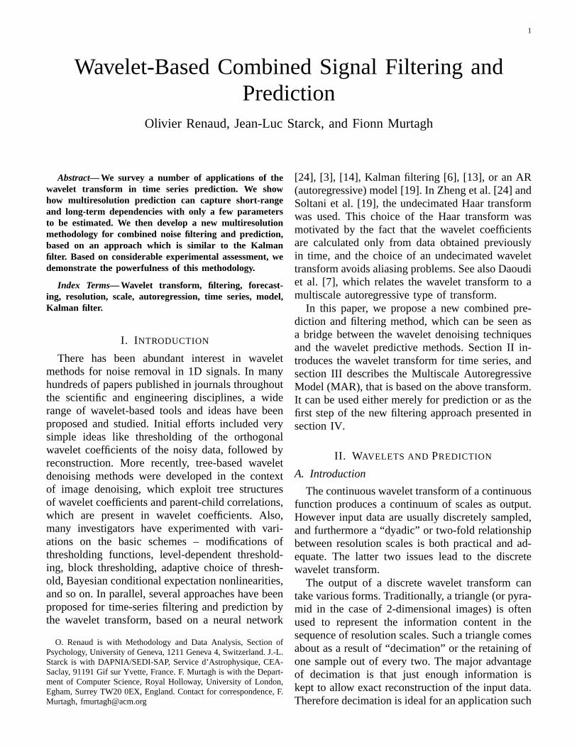
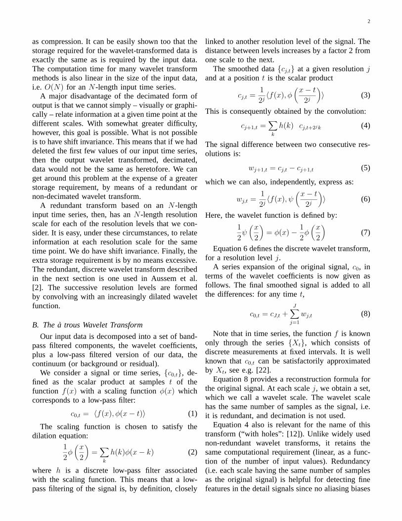
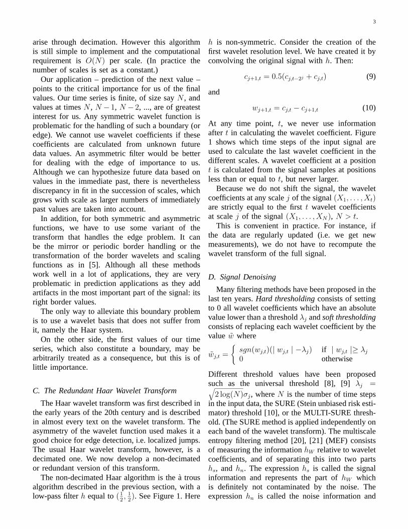
The non-decimated Haar algorithm is thea trousalgorithm described in the previous section, with alow-pass filterh equal to(1

2, 1

2). See Figure 1. Here

h is non-symmetric. Consider the creation of thefirst wavelet resolution level. We have created it byconvolving the original signal withh. Then:

cj+1,t = 0.5(cj,t−2j + cj,t) (9)

and

wj+1,t = cj,t − cj+1,t (10)

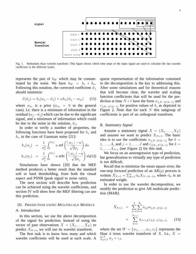
At any time point, t, we never use informationafter t in calculating the wavelet coefficient. Figure1 shows which time steps of the input signal areused to calculate the last wavelet coefficient in thedifferent scales. A wavelet coefficient at a positiont is calculated from the signal samples at positionsless than or equal tot, but never larger.

Because we do not shift the signal, the waveletcoefficients at any scalej of the signal(X1, . . . , Xt)are strictly equal to the firstt wavelet coefficientsat scalej of the signal(X1, . . . , XN), N > t.

This is convenient in practice. For instance, ifthe data are regularly updated (i.e. we get newmeasurements), we do not have to recompute thewavelet transform of the full signal.

D. Signal Denoising

Many filtering methods have been proposed in thelast ten years.Hard thresholdingconsists of settingto 0 all wavelet coefficients which have an absolutevalue lower than a thresholdλj andsoft thresholdingconsists of replacing each wavelet coefficient by thevalue w where

wj,t =

{

sgn(wj,t)(| wj,t | −λj) if | wj,t |≥ λj

0 otherwise

Different threshold values have been proposedsuch as the universal threshold [8], [9]λj =√

2 log(N)σj, whereN is the number of time stepsin the input data, the SURE (Stein unbiased risk esti-mator) threshold [10], or the MULTI-SURE thresh-old. (The SURE method is applied independently oneach band of the wavelet transform). The multiscaleentropy filtering method [20], [21] (MEF) consistsof measuring the informationhW relative to waveletcoefficients, and of separating this into two partshs, andhn. The expressionhs is called the signalinformation and represents the part ofhW whichis definitely not contaminated by the noise. Theexpressionhn is called the noise information and

4

signal

scale 1

scale 2

scale 3

scale 4

smooth array

WaveletTransform

Fig. 1. Redundant Haar wavelet transform: This figure shows which time steps of the input signal are used to calculate the last waveletcoefficient in the different scales.

represents the part ofhW which may be contam-inated by the noise. We havehW = hs + hn.Following this notation, the corrected coefficientwj

should minimize:

J(wj) = hs(wj − wj) + αhn(wj − wm) (11)

where wm is a prior (wm = 0 in the generalcase). I.e. there is a minimum of information in theresidual (wj−wj) which can be due to the significantsignal, and a minimum of information which couldbe due to the noise in the solution,wj.

In order to verify a number of properties, thefollowing functions have been proposed forhs andhn in the case of Gaussian noise [21]:

hs(wj) =1

σ2j

∫ |wj |

0u erf

(

| wj | −u√2σj

)

du

hn(wj) =1

σ2j

∫ |wj |

0u erfc

(

| wj | −u√2σj

)

du(12)

Simulations have shown [20] that the MEFmethod produces a better result than the standardsoft or hard thresholding, from both the visualaspect and PSNR (peak signal to noise ratio).

The next section will describe how predictioncan be achieved using the wavelet coefficients, andsection IV will show how the MEF filtering can usethis prediction.

III. PREDICTION USINGMULTISCALE MODELS

A. Introduction

In this section, we use the above decompositionof the signal for prediction. Instead of using thevector of past observationsX = (X1, . . . , XN) topredictXN+1, we will use its wavelet transform.

The first task is to know how many and whichwavelet coefficients will be used at each scale. A

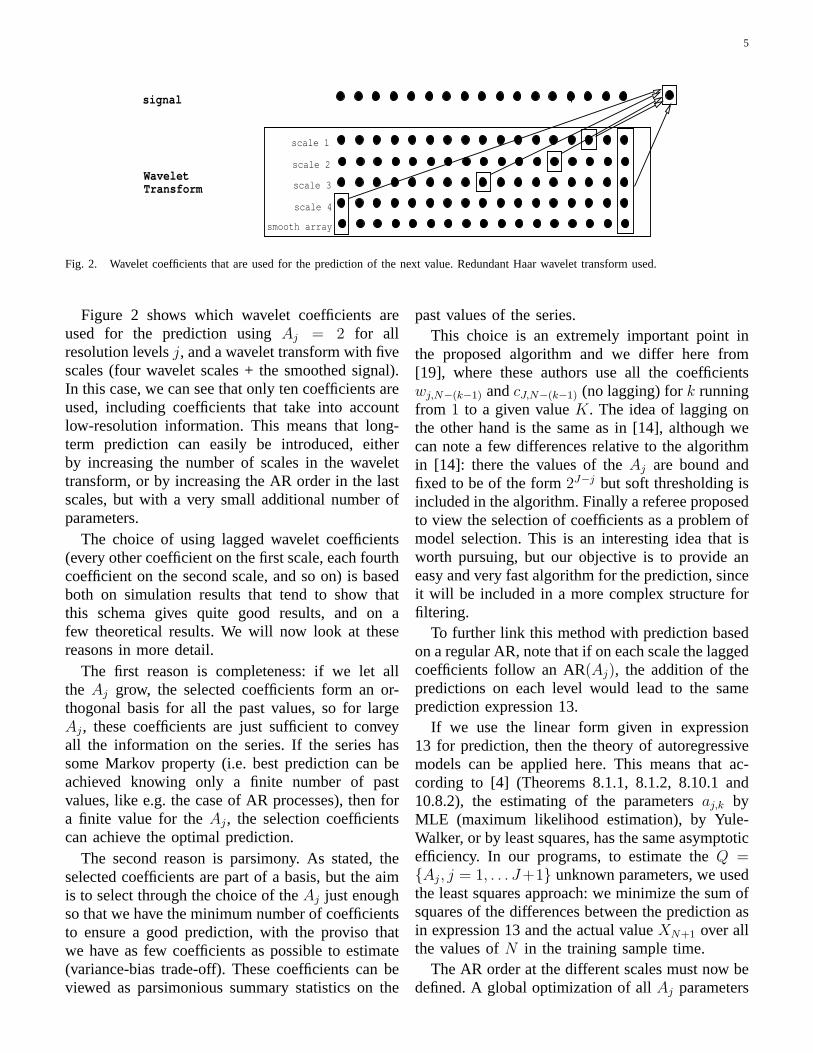
sparse representation of the information containedin the decomposition is the key to addressing this.After some simulations and for theoretical reasonsthat will become clear, the wavelet and scalingfunction coefficients that will be used for the pre-diction at timeN+1 have the formwj,N−2j(k−1) andcJ,N−2J (k−1) for positive values ofk, as depicted inFigure 2. Note that for eachN this subgroup ofcoefficients is part of an orthogonal transform.

B. Stationary Signal

Assume a stationary signalX = (X1, . . . , XN)and assume we want to predictXN+1. The basicidea is to use the coefficientswj,N−2j(k−1) for k =1, . . . , Aj andj = 1, . . . , J andcJ,N−2J (k−1) for k =1, . . . , AJ+1 (see Figure 2) for this task.

We focus on an autoregressive type of prediction,but generalization to virtually any type of predictionis not difficult.

Recall that to minimize the mean square error, theone-step forward prediction of an AR(p) process iswritten XN+1 =

∑pk=1 αkXN−(k−1), whereαk is an

estimated weight.In order to use the wavelet decomposition, we

modify the prediction to give AR multiscale predic-tion (MAR):

XN+1 =J∑

j=1

Aj∑

k=1

aj,kwj,N−2j(k−1)

+AJ+1∑

k=1

aJ+1,kcJ,N−2J (k−1) (13)

where the setW = {w1, . . . , wJ , cJ} represents theHaar a trous wavelet transform ofX. I.e., X =∑J

j=1wj + cJ .

5

signal

scale 1

scale 2

scale 3

scale 4

smooth array

WaveletTransform

Fig. 2. Wavelet coefficients that are used for the prediction of the next value. Redundant Haar wavelet transform used.

Figure 2 shows which wavelet coefficients areused for the prediction usingAj = 2 for allresolution levelsj, and a wavelet transform with fivescales (four wavelet scales + the smoothed signal).In this case, we can see that only ten coefficients areused, including coefficients that take into accountlow-resolution information. This means that long-term prediction can easily be introduced, eitherby increasing the number of scales in the wavelettransform, or by increasing the AR order in the lastscales, but with a very small additional number ofparameters.

The choice of using lagged wavelet coefficients(every other coefficient on the first scale, each fourthcoefficient on the second scale, and so on) is basedboth on simulation results that tend to show thatthis schema gives quite good results, and on afew theoretical results. We will now look at thesereasons in more detail.

The first reason is completeness: if we let allthe Aj grow, the selected coefficients form an or-thogonal basis for all the past values, so for largeAj, these coefficients are just sufficient to conveyall the information on the series. If the series hassome Markov property (i.e. best prediction can beachieved knowing only a finite number of pastvalues, like e.g. the case of AR processes), then fora finite value for theAj, the selection coefficientscan achieve the optimal prediction.

The second reason is parsimony. As stated, theselected coefficients are part of a basis, but the aimis to select through the choice of theAj just enoughso that we have the minimum number of coefficientsto ensure a good prediction, with the proviso thatwe have as few coefficients as possible to estimate(variance-bias trade-off). These coefficients can beviewed as parsimonious summary statistics on the

past values of the series.This choice is an extremely important point in

the proposed algorithm and we differ here from[19], where these authors use all the coefficientswj,N−(k−1) andcJ,N−(k−1) (no lagging) fork runningfrom 1 to a given valueK. The idea of lagging onthe other hand is the same as in [14], although wecan note a few differences relative to the algorithmin [14]: there the values of theAj are bound andfixed to be of the form2J−j but soft thresholding isincluded in the algorithm. Finally a referee proposedto view the selection of coefficients as a problem ofmodel selection. This is an interesting idea that isworth pursuing, but our objective is to provide aneasy and very fast algorithm for the prediction, sinceit will be included in a more complex structure forfiltering.

To further link this method with prediction basedon a regular AR, note that if on each scale the laggedcoefficients follow an AR(Aj), the addition of thepredictions on each level would lead to the sameprediction expression 13.

If we use the linear form given in expression13 for prediction, then the theory of autoregressivemodels can be applied here. This means that ac-cording to [4] (Theorems 8.1.1, 8.1.2, 8.10.1 and10.8.2), the estimating of the parametersaj,k byMLE (maximum likelihood estimation), by Yule-Walker, or by least squares, has the same asymptoticefficiency. In our programs, to estimate theQ ={Aj, j = 1, . . . J+1} unknown parameters, we usedthe least squares approach: we minimize the sum ofsquares of the differences between the prediction asin expression 13 and the actual valueXN+1 over allthe values ofN in the training sample time.

The AR order at the different scales must now bedefined. A global optimization of allAj parameters

6

would be the ideal method, but is too computerintensive. However, by the relative non-overlappingfrequencies used in each scale, we can considerselecting the parametersAj independently on eachscale. This can be done by standard methods, basedon AIC, AICC or BIC methods [18].

C. Non-linear and Non-stationary Generalizations

This Multiresolution AR prediction model is ac-tually linear. To go beyond this, we can imagineusing virtually any type of prediction, linear or non-linear, that uses the previous dataXN , . . . , XN−q

and generalize it through the use of the coefficientswj,t andcJ,t, t ≤ N instead.

One example is to feed a multilayer perceptronneural network with these coefficientsw and c asinputs, use one or more hidden layer(s), and obtainXN+1 as the (unique) output, as has been done in[15]. In this case, a backpropagation algorithm canbe used for the estimation of the parameters.

We can also think of using a model that allowsfor some form of non-stationarity. For example wecould use an ARCH or GARCH model on eachscale to model the conditional heteroscedasticityoften present in financial data.

Finally, if we stay with the linear MAR, it is easyto change slightly the algorithm to handle signalwith a piecewise smooth trend. We show in [16]how to extend this method, and to take advantageof the last smooth signal to estimate it.

D. Assessments on Real Data

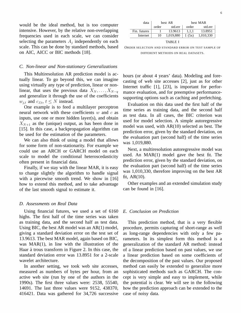
Using financial futures, we used a set of 6160highs. The first half of the time series was takenas training data, and the second half as test data.Using BIC, the best AR model was an AR(1) model,giving a standard deviation error on the test set of13.9613. The best MAR model, again based on BIC,was MAR(1), in line with the illustration of theHaara trous transform in Figure 2. In this case, thestandard deviation error was 13.8951 for a 2-scalewavelet architecture.

In another setting, we took web site accesses,measured as numbers of bytes per hour, from anactive web site (run by one of the authors in the1990s). The first three values were: 2538, 55540,14691. The last three values were 9152, 438370,416421. Data was gathered for 34,726 successive

data best AR best MARorder std.err order std.err

Fin. futures 1 13.9613 1,1,1 13.8951Internet 10 1,019,880 1 (5x) 1,010,330

TABLE I

ORDER SELECTION AND STANDARD ERROR ON TEST SAMPLE OF

DIFFERENT METHODS ON REAL DATASETS.

hours (or about 4 years’ data). Modeling and fore-casting of web site accesses [2], just as for otherInternet traffic [1], [23], is important for perfor-mance evaluation, and for preemptive performance-supporting options such as caching and prefetching.

Evaluation on this data used the first half of thetime series as training data, and the second halfas test data. In all cases, the BIC criterion wasused for model selection. A simple autoregressivemodel was used, with AR(10) selected as best. Theprediction error, given by the standard deviation, onthe evaluation part (second half) of the time serieswas 1,019,880.

Next, a multiresolution autoregressive model wasused. An MAR(1) model gave the best fit. Theprediction error, given by the standard deviation, onthe evaluation part (second half) of the time serieswas 1,010,330, therefore improving on the best ARfit, AR(10).

Other examples and an extended simulation studycan be found in [16].

E. Conclusion on Prediction

This prediction method, that is a very flexibleprocedure, permits capturing of short-range as wellas long-range dependencies with only a few pa-rameters. In its simplest form this method is ageneralization of the standard AR method: insteadof a linear prediction based on past values, we usea linear prediction based on some coefficients ofthe decomposition of the past values. Our proposedmethod can easily be extended to generalize moresophisticated methods such as GARCH. The con-cept is very simple and easy to implement, whilethe potential is clear. We will see in the followinghow the prediction approach can be extended to thecase of noisy data.

7

IV. F ILTERING USING THE MULTISCALE

PREDICTION

A. Introduction

In this section, we show how to execute the pre-diction and filtering in the wavelet domain to takeadvantage of the decomposition. We will considerstochastic signals measured with an error noise.Therefore the type of equations that are believed todrive the signal can be expressed as the followingmeasurement and transition equations:

yN+1 = ZN+1xN+1 + vN+1 (14)

xN+1 = function(xN) + ǫN+1, (15)

where thevt are IID N (0,Σv), the ǫt are zero-mean noise, and thevt are independent of theǫt.The process{xt} has a stochastic behavior, but wemeasure it only through{yt}, which is essentiallya noisy version of it. Data that seem to follow thiskind of equation can be found in many differentfields of science, since error in measurement is morethe rule than the exception. The aim is clearly to bestpredict the future value of the underlying processxN+1, based on the observed valuesy.

Solving these equations and finding the best pre-diction and the best filtered value at each time pointseem difficult and computer intensive. However ina special case of equations 14 and 15, the Kalmanfilter gives rise to an algorithm that is easy toimplement and that is very efficient, since the futurepredicted and filtered values are only based on thepresent values, and depend on the past values onlythrough a pair of matrices that are updated at eachtime point. This method supposes in addition to theprevious equation thatxN+1 = TN+1xN +ǫN+1, thatboth errors are Gaussian,vt areN (0,Σv) andǫt areN (0,Σe), and thatZt, Σv, Tt and Σe are known.The Kalman filter gives a recursive construction ofthe predicted and filtered values which has optimalproperties. The predicted (p) and filtered (f ) valuesof xN+1 are given by the coupled recurrence:

pN+1 = TN+1fN (16)

fN+1 = pN+1 +KN+1(yN+1 − ZN+1pN+1) (17)

whereKN+1 is the gain matrix that is also given bya recursive scheme and depends onZN+1, Σv, TN+1

andΣe (see [11], [17]). Ifvt andǫt, t ≤ N +1, areGaussian,pN+1 is the best prediction in the sensethat it minimizes the mean square error given the

past values (= E(xN+1|y1, . . . ,yN)) and fN+1 isthe best filter in the sense that it minimizes themean square error given all values up toN + 1(= E(xN+1|y1, . . . ,yN+1)). If the errors are notGaussian, the estimators are optimal within the classof linear estimators, see [11].

Under Gaussianity of the errors, ifΣv, Tt andΣe

are known only up to a given number of param-eters, the maximum likelihood of the innovationscan be stated and either a Newton-Raphson or anEM (expectation-maximization) algorithm can beused to minimize the likelihood which is severelynon-linear in the unknown parameters, and givesestimates for these parameters.

B. Filtering

In this work we propose a method similar to theKalman filter but that allows two generalizations onthe type of equation that can be treated. The first oneis to allow for different functions in the transitionequation 15. The versatility of the wavelet transformand the freedom to choose the prediction formallow for very general function approximation. Thesecond generalization is to allow the noise of thetransition equationǫt to be non-Gaussian and evento have some very large values. Using multiscaleentropy filtering, these cases will be detected andthe filtering will not be misled.

Like in the Kalman filter, we define a recurrencescheme to obtain the predicted values and the fil-tered values. This allows us to have a fast algorithmthat does not have to recompute all estimations ateach new value. However, the recurrence equationswill not be linear as in the Kalman filter and theywill not be based on the values themselves, but willbe carried out in the wavelet domain.

For notational convenience, we present ourmethod for a simplified equation wherext is uni-dimensional andZt is equal to 1 for allt ≤ N .For the prediction part, instead of using the vectorof past filtered valuesf = (f1, . . . , fN) to predictpN+1, as in 16, we will use its wavelet transform.

It has been shown previously that the waveletand scaling function coefficients that must be usedfor the prediction at timeN + 1 have the formwf

j,N−2j(k−1) and cfJ,N−2J (k−1) for positive values of

k. Given the wavelet decomposition of the filteredvalues ft, wf and cf , we predict the next valuebased on the Multiresolution Autoregressive (MAR)model

8

pN+1 =J∑

j=1

Aj∑

k=1

aj,kwf

j,N−2j(k−1)

+AJ+1∑

k=1

aJ+1,kcf

J,N−2J (k−1) (18)

where the setW = {wf1 , . . . , w

fJ , c

fJ} represents

the Haara trous wavelet transform off , and wehave:f =

∑Jj=1w

fj + cfJ . Again, depending on the

supposed process that generated the data, we canimagine other prediction equations based on thesecoefficients, like Multiresolution Neural Network(MNN), Multiresolution GARCH, and so on.

This first part of the algorithm has the same roleas equation 16 for the Kalman filter. Given thefiltered values up to timeN , ft, t = 1, . . . , N ,and its Haara trous wavelet transformwf

j,t fort = 1, . . . , N and j = 1, . . . , J , and cfJ,t for t =1, . . . , N , we use the wavelet decomposition offt

to predict the next valuepN+1. The difference withKalman is the form of the prediction: it is basedon the multiresolution decomposition and might benon-linear if so desired.

For the second part of the algorithm, like theKalman filtering equation 17, we will compare theobserved valueyN+1 and the predicted valuepN+1,but in the wavelet domain. From the predicted valuepN+1 we decompose in the wavelet domain (with –some of – the previous filtered values up tofN ) toobtain theJ+1 coefficientswp

j,N+1 for j = 1, . . . , JandcpJ,N+1. For the filtering part, we first decomposethe new observationyN+1 in the wavelet domain(using also the previous observationsyt) to obtainthe J + 1 coefficientswy

j,N+1 for j = 1, . . . , J andcyJ,N+1.

Informally, the Kalman filter computes a filteredvaluefN+1 on the basis of the predicted valuepN+1

and corrects it only if the new observation is farfrom its predicted value. Here we work on thewavelet coefficients and we will also set the filteredvalue as close to the predicted value, unless theprediction is far from the actual coefficient. To carryout the compromise, we use the multiscale entropygiven in expression 11, and tailor it to the situation.The wavelet coefficient of the filtered value will bethe one that satisfies

minw

f

j,N+1

hs

wyj,N+1 − wf

j,N+1

σv

+λhn

wfj,N+1 − wp

j,N+1

σe

(19)

and similarly for the smooth arraycfJ,N+1. The coef-ficientwf

j,N+1 must be close to the same coefficientfor the measured signaly and at the same time closeto the predicted valuewp

j,N+1. Since the standarderrors of the noisevt andǫt in equations 14 and 15can be very different, we have to standardize bothdifferences in 19. Note thatλ plays the role of thetrade-off parameter between the prediction and thenew value. This can be viewed as the thresholdingconstant in the regression context. Having obtainedthe filtered coefficients for all scales, we can simplyrecoverfN+1 with equation 8.

This algorithm with the Multiresolution AR is ofthe same complexity as the Kalman filter, since thea trous transform is of linear order. If one considersthe number of scales as a (necessarily logarithmic)function of the number of observations, an addi-tional factor of log(N) is found in the complexity.The key to this lies in the fact that we do notrecompute the entirea trous transform off , p ory each time a new value is added, but we computeonly theJ+1 coefficientswj,t for j = 1, . . . , J andcJ,t at a given timet. If one uses a more complexprediction scheme, like a neural network, then thecomplexity of our algorithm is driven by this pre-diction algorithm. The proposed algorithm is alsosimple, thanks to the Haar transform (equations 8,9 and 10) which is especially easy to implement.

The estimation of the unknown parameters fol-lows the same lines as for prediction, although theestimation of the noise levels is known to be a moredifficult task. The key to the performance of themethod in the pure prediction case was to allowit to adapt the numberAj of coefficients kept ateach scale for the prediction. This was done usinga penalization criterion such as BIC. We believethat it is important to do exactly the same in thefiltering framework. We refer to Section III for theseparameters. The estimation ofσv, σe andλ is moredelicate, and in our programs, we leave the choice tothe user either to provide these values or to let thembe estimated. Of course, when the true values for

9

the standard deviations are known independently,the method is more effective, but we note that evenif the algorithm over- or underestimates these valuesup to 50%, performance is still good.

First, the optimalλ is strongly related to thetwo standard deviations, and more precisely to theirratio. In our simulations, we setλ to be0.1σv/σe.

The leading parameter here isσv, since it drivesall the smoothing, and once this parameter has beenset or estimated, the procedure proceeds as in theprediction case. If the program has to estimate thisparameter, a grid of 30 different values forσv istried, from zero to the standard deviation of theobserved datay. The resulting models are comparedon the innovation error and we select the one thatminimizes the error. We could use a more complexalgorithm that refines the grid close to the minimalvalues, but we do not believe that this will improvethe model in a significant way. On the contrary, wehave found that this method is relatively robust tothe parameter estimation and that there is an intervalof values that leads to the same standard deviationof error.

V. SIMULATIONS

A. Experiment 1

In this section, we use a Monte-Carlo study tocompare the proposed filtered method with the reg-ular Kalman filter. The first two simulation studieshave models where Kalman is known to be optimal.The aim is to see whether the multiresolution ap-proach is able to get close to this “gold standard” inthis special case. The second part uses a much moredifficult model (ARFIMA plus noise) where Kalmanis not optimal any more. We will be interested inthe deterioration of performance of both methods.

In the first case, we generated processes{Xt} thatfollow a causal AR process of orderp, which meansthat they satisfyXt = φ1Xt−1 + · · · + φpXt−p + ǫt.We measure onlyYt which is a noisy version ofthis process:Yt = Xt + vt. Both noises are takento be Gaussian, i.e.{ǫt} areN (0, σ2

e) and{vt} areN (0, σ2

v). For any value ofp this process can bewritten in the Kalman form of equations 14 and 15,with a p-dimensionalxt [11].

We compare 5 different filtering algorithms. First,True Kal is the oracular Kalman filter that has beenfed with the true values of all parameters: the ARorderp and the values ofφi, σe andσv. This is the

unattainable best filter. Second isEstim.Kal whichis a Kalman filter that has been fed with the trueAR order p but we have to estimate the values ofφi, σe andσv. This is done through the likelihood ofthe innovations [17]. It is well known that the mostdifficult parameters to estimate are the estimates ofboth variabilitiesσe and σv. So the third methodEst.AR.Kal is again a Kalman filter which has beenfed with p, σe andσv, and has only to estimate theφ’s. Note that these three Kalman methods are fedwith the true orderp. If they had to select it via acriterion, we could expect significant deteriorationin their performance. The fourth methodObser isthe simplistic choice not to do any filtering and toprovide yt as being the best estimate forxt. If amethod gives results that are worse thanObser,it has clearly missed the target. It is however notan easy task whenσv is small. The last approach,MultiRes, is our proposed method, with 5 scales asin prediction, and with the level of the measurementnoise that is given. So, contrary to the three Kalmanfilters, the method is not fed with the true order,but has to select it levelwise with the BIC criterion.However, likeEst.AR.Kal, the method is fed withσv.

The 50 series are of length 1000 and the first500 points are used for training and the last 500 areused to compare the standard deviation of the errorbetween the filtered and the true values. A boxplotgives in the center the median value for the responseand the box contains 50% of the responses, givingan idea of the variability between the samples.Hence the best method is the one for which theboxplot is the most stumpy and compact.

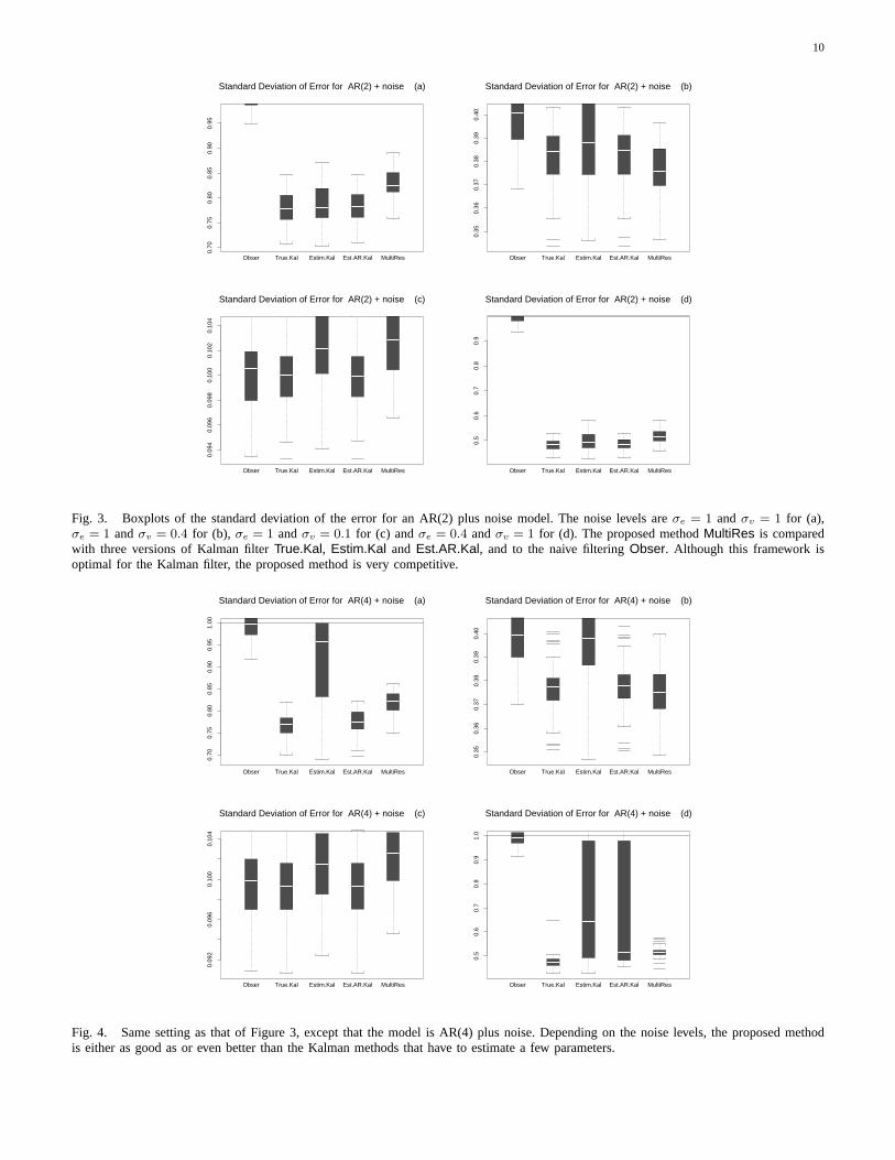
For Figure 3 the AR order isp = 2 with parame-terφ′ = (0.5,−0.7). The noise levels are as follows:for subplot (a)σe = 1 andσv = 1, for subplot (b)σe = 1 and σv = 0.4, for subplot (c)σe = 1 andσv = 0.1 and finally for subplot (d)σe = 0.4 andσv = 1. In all cases, theTrue.Kal method shouldbe the best one. In addition, in case (c) where themeasurement error is very small, the simpleObsershould be competitive or even difficult to beat. Thisis in fact the case. In addition, the proposed methodMultiRes has standard deviations of the errors al-most as good as the oracularTrue.Kal, and is verycompetitive withEstim.Kal andEst.AR.Kal, whichare both based on the correct Kalman filter but haveto estimate some parameters.

The second simulation, the results of which are

10

0.70

0.75

0.80

0.85

0.90

0.95

Obser True.Kal Estim.Kal Est.AR.Kal MultiRes

Standard Deviation of Error for AR(2) + noise (a)

0.35

0.36

0.37

0.38

0.39

0.40

Obser True.Kal Estim.Kal Est.AR.Kal MultiRes

Standard Deviation of Error for AR(2) + noise (b)

0.09

40.

096

0.09

80.

100

0.10

20.

104

Obser True.Kal Estim.Kal Est.AR.Kal MultiRes

Standard Deviation of Error for AR(2) + noise (c)

0.5

0.6

0.7

0.8

0.9

Obser True.Kal Estim.Kal Est.AR.Kal MultiRes

Standard Deviation of Error for AR(2) + noise (d)

Fig. 3. Boxplots of the standard deviation of the error for an AR(2) plus noise model. The noise levels areσe = 1 and σv = 1 for (a),σe = 1 andσv = 0.4 for (b), σe = 1 andσv = 0.1 for (c) andσe = 0.4 andσv = 1 for (d). The proposed methodMultiRes is comparedwith three versions of Kalman filterTrue.Kal, Estim.Kal and Est.AR.Kal, and to the naive filteringObser. Although this framework isoptimal for the Kalman filter, the proposed method is very competitive.

0.70

0.75

0.80

0.85

0.90

0.95

1.00

Obser True.Kal Estim.Kal Est.AR.Kal MultiRes

Standard Deviation of Error for AR(4) + noise (a)

0.35

0.36

0.37

0.38

0.39

0.40

Obser True.Kal Estim.Kal Est.AR.Kal MultiRes

Standard Deviation of Error for AR(4) + noise (b)

0.09

20.

096

0.10

00.

104

Obser True.Kal Estim.Kal Est.AR.Kal MultiRes

Standard Deviation of Error for AR(4) + noise (c)

0.5

0.6

0.7

0.8

0.9

1.0

Obser True.Kal Estim.Kal Est.AR.Kal MultiRes

Standard Deviation of Error for AR(4) + noise (d)

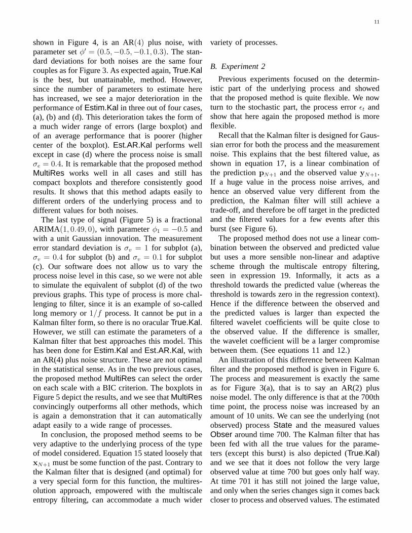
Fig. 4. Same setting as that of Figure 3, except that the model is AR(4) plus noise. Depending on the noise levels, the proposed methodis either as good as or even better than the Kalman methods that have to estimate a few parameters.

11

shown in Figure 4, is an AR(4) plus noise, withparameter setφ′ = (0.5,−0.5,−0.1, 0.3). The stan-dard deviations for both noises are the same fourcouples as for Figure 3. As expected again,True.Kalis the best, but unattainable, method. However,since the number of parameters to estimate herehas increased, we see a major deterioration in theperformance ofEstim.Kal in three out of four cases,(a), (b) and (d). This deterioration takes the form ofa much wider range of errors (large boxplot) andof an average performance that is poorer (highercenter of the boxplot).Est.AR.Kal performs wellexcept in case (d) where the process noise is smallσe = 0.4. It is remarkable that the proposed methodMultiRes works well in all cases and still hascompact boxplots and therefore consistently goodresults. It shows that this method adapts easily todifferent orders of the underlying process and todifferent values for both noises.

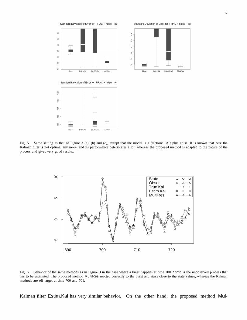
The last type of signal (Figure 5) is a fractionalARIMA (1, 0.49, 0), with parameterφ1 = −0.5 andwith a unit Gaussian innovation. The measurementerror standard deviation isσv = 1 for subplot (a),σv = 0.4 for subplot (b) andσv = 0.1 for subplot(c). Our software does not allow us to vary theprocess noise level in this case, so we were not ableto simulate the equivalent of subplot (d) of the twoprevious graphs. This type of process is more chal-lenging to filter, since it is an example of so-calledlong memory or1/f process. It cannot be put in aKalman filter form, so there is no oracularTrue.Kal.However, we still can estimate the parameters of aKalman filter that best approaches this model. Thishas been done forEstim.Kal andEst.AR.Kal, withan AR(4) plus noise structure. These are not optimalin the statistical sense. As in the two previous cases,the proposed methodMultiRes can select the orderon each scale with a BIC criterion. The boxplots inFigure 5 depict the results, and we see thatMultiResconvincingly outperforms all other methods, whichis again a demonstration that it can automaticallyadapt easily to a wide range of processes.

In conclusion, the proposed method seems to bevery adaptive to the underlying process of the typeof model considered. Equation 15 stated loosely thatxN+1 must be some function of the past. Contrary tothe Kalman filter that is designed (and optimal) fora very special form for this function, the multires-olution approach, empowered with the multiscaleentropy filtering, can accommodate a much wider

variety of processes.

B. Experiment 2

Previous experiments focused on the determin-istic part of the underlying process and showedthat the proposed method is quite flexible. We nowturn to the stochastic part, the process errorǫt andshow that here again the proposed method is moreflexible.

Recall that the Kalman filter is designed for Gaus-sian error for both the process and the measurementnoise. This explains that the best filtered value, asshown in equation 17, is a linear combination ofthe predictionpN+1 and the observed valueyN+1.If a huge value in the process noise arrives, andhence an observed value very different from theprediction, the Kalman filter will still achieve atrade-off, and therefore be off target in the predictedand the filtered values for a few events after thisburst (see Figure 6).

The proposed method does not use a linear com-bination between the observed and predicted valuebut uses a more sensible non-linear and adaptivescheme through the multiscale entropy filtering,seen in expression 19. Informally, it acts as athreshold towards the predicted value (whereas thethreshold is towards zero in the regression context).Hence if the difference between the observed andthe predicted values is larger than expected thefiltered wavelet coefficients will be quite close tothe observed value. If the difference is smaller,the wavelet coefficient will be a larger compromisebetween them. (See equations 11 and 12.)

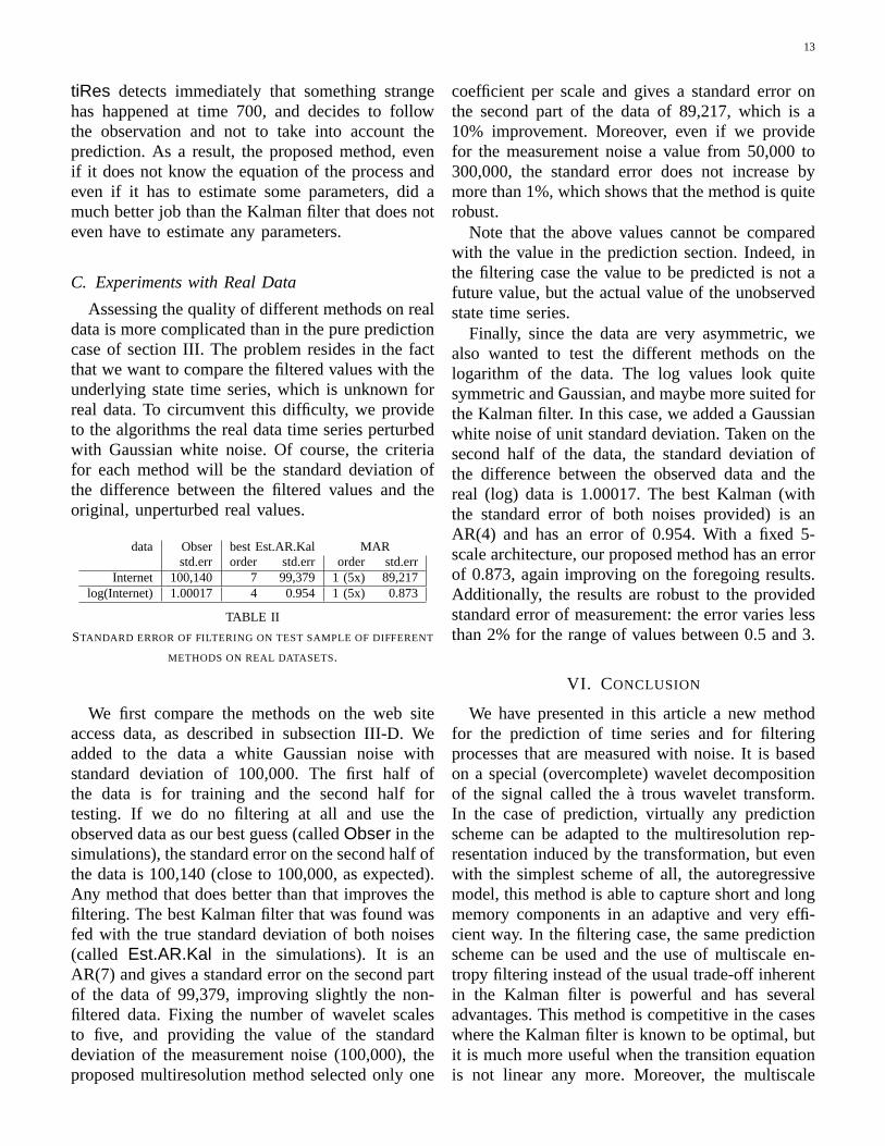
An illustration of this difference between Kalmanfilter and the proposed method is given in Figure 6.The process and measurement is exactly the sameas for Figure 3(a), that is to say an AR(2) plusnoise model. The only difference is that at the 700thtime point, the process noise was increased by anamount of 10 units. We can see the underlying (notobserved) processState and the measured valuesObser around time 700. The Kalman filter that hasbeen fed with all the true values for the parame-ters (except this burst) is also depicted (True.Kal)and we see that it does not follow the very largeobserved value at time 700 but goes only half way.At time 701 it has still not joined the large value,and only when the series changes sign it comes backcloser to process and observed values. The estimated

12

0.7

0.8

0.9

1.0

1.1

1.2

1.3

Obser Estim.Kal Est.AR.Kal MultiRes

Standard Deviation of Error for FRAC + noise (a)

0.4

0.5

0.6

0.7

0.8

0.9

Obser Estim.Kal Est.AR.Kal MultiRes

Standard Deviation of Error for FRAC + noise (b)

0.10

0.12

0.14

0.16

0.18

Obser Estim.Kal Est.AR.Kal MultiRes

Standard Deviation of Error for FRAC + noise (c)

Fig. 5. Same setting as that of Figure 3 (a), (b) and (c), except that themodel is a fractional AR plus noise. It is known that here theKalman filter is not optimal any more, and its performance deteriorates a lot, whereas the proposed method is adapted to the nature of theprocess and gives very good results.

690 700 710 720

−50

510 State

ObserTrue KalEstim KalMultiRes

Fig. 6. Behavior of the same methods as in Figure 3 in the case where a burst happens at time 700.State is the unobserved process thathas to be estimated. The proposed methodMultiRes reacted correctly to the burst and stays close to the state values, whereasthe Kalmanmethods are off target at time 700 and 701.

Kalman filterEstim.Kal has very similar behavior. On the other hand, the proposed method Mul-

13

tiRes detects immediately that something strangehas happened at time 700, and decides to followthe observation and not to take into account theprediction. As a result, the proposed method, evenif it does not know the equation of the process andeven if it has to estimate some parameters, did amuch better job than the Kalman filter that does noteven have to estimate any parameters.

C. Experiments with Real Data

Assessing the quality of different methods on realdata is more complicated than in the pure predictioncase of section III. The problem resides in the factthat we want to compare the filtered values with theunderlying state time series, which is unknown forreal data. To circumvent this difficulty, we provideto the algorithms the real data time series perturbedwith Gaussian white noise. Of course, the criteriafor each method will be the standard deviation ofthe difference between the filtered values and theoriginal, unperturbed real values.

data Obser best Est.AR.Kal MARstd.err order std.err order std.err

Internet 100,140 7 99,379 1 (5x) 89,217log(Internet) 1.00017 4 0.954 1 (5x) 0.873

TABLE II

STANDARD ERROR OF FILTERING ON TEST SAMPLE OF DIFFERENT

METHODS ON REAL DATASETS.

We first compare the methods on the web siteaccess data, as described in subsection III-D. Weadded to the data a white Gaussian noise withstandard deviation of 100,000. The first half ofthe data is for training and the second half fortesting. If we do no filtering at all and use theobserved data as our best guess (calledObser in thesimulations), the standard error on the second half ofthe data is 100,140 (close to 100,000, as expected).Any method that does better than that improves thefiltering. The best Kalman filter that was found wasfed with the true standard deviation of both noises(called Est.AR.Kal in the simulations). It is anAR(7) and gives a standard error on the second partof the data of 99,379, improving slightly the non-filtered data. Fixing the number of wavelet scalesto five, and providing the value of the standarddeviation of the measurement noise (100,000), theproposed multiresolution method selected only one

coefficient per scale and gives a standard error onthe second part of the data of 89,217, which is a10% improvement. Moreover, even if we providefor the measurement noise a value from 50,000 to300,000, the standard error does not increase bymore than 1%, which shows that the method is quiterobust.

Note that the above values cannot be comparedwith the value in the prediction section. Indeed, inthe filtering case the value to be predicted is not afuture value, but the actual value of the unobservedstate time series.

Finally, since the data are very asymmetric, wealso wanted to test the different methods on thelogarithm of the data. The log values look quitesymmetric and Gaussian, and maybe more suited forthe Kalman filter. In this case, we added a Gaussianwhite noise of unit standard deviation. Taken on thesecond half of the data, the standard deviation ofthe difference between the observed data and thereal (log) data is 1.00017. The best Kalman (withthe standard error of both noises provided) is anAR(4) and has an error of 0.954. With a fixed 5-scale architecture, our proposed method has an errorof 0.873, again improving on the foregoing results.Additionally, the results are robust to the providedstandard error of measurement: the error varies lessthan 2% for the range of values between 0.5 and 3.

VI. CONCLUSION

We have presented in this article a new methodfor the prediction of time series and for filteringprocesses that are measured with noise. It is basedon a special (overcomplete) wavelet decompositionof the signal called thea trous wavelet transform.In the case of prediction, virtually any predictionscheme can be adapted to the multiresolution rep-resentation induced by the transformation, but evenwith the simplest scheme of all, the autoregressivemodel, this method is able to capture short and longmemory components in an adaptive and very effi-cient way. In the filtering case, the same predictionscheme can be used and the use of multiscale en-tropy filtering instead of the usual trade-off inherentin the Kalman filter is powerful and has severaladvantages. This method is competitive in the caseswhere the Kalman filter is known to be optimal, butit is much more useful when the transition equationis not linear any more. Moreover, the multiscale

14

entropy filtering is robust relative to Gaussianity ofthe transition noise.

REFERENCES

[1] P. Abry, D. Veitch, and P. Flandrin. Long-range dependence:revisting aggregation with wavelets.Journal of Time SeriesAnalysis, 19:253–266, 1998.

[2] A. Aussem and F. Murtagh. A neuro-wavelet strategy for webtraffic forecasting.Journal of Official Statistics, 1:65–87, 1998.

[3] Z. Bashir and M.E. El-Hawary. Short term load forecastingby using wavelet neural networks. InCanadian Conference onElectrical and Computer Engineering, pages 163–166, 2000.

[4] P.J. Brockwell and R.A. Davis. Time Series: Theory andMethods. Springer-Verlag, 1991.

[5] A. Cohen, I. Daubechies, and J. Feauveau. Bi-orthogonal basesof compactly supported wavelets.Comm. Pure and Appl. Math.,45:485–560, 1992.

[6] R. Cristi and M. Tummula. Multirate, multiresolution, recursiveKalman filter. Signal Processing, 80:1945–1958, 2000.

[7] K. Daoudi, A.B. Frakt, and A.S. Willsky. Multiscale autoregres-sive models and wavelets.IEEE Transactions on InformationTheory, 45(3):828–845, 1999.

[8] D.L. Donoho. Nonlinear wavelet methods for recovery ofsignals, densities, and spectra from indirect and noisy data. InProceedings of Symposia in Applied Mathematics, volume 47,pages 173–205. American Mathematical Society, 1993.

[9] D.L. Donoho and I.M. Johnstone. Ideal spatial adaptation viawavelet shrinkage.Biometrika, 81:425–455, 1994.

[10] D.L. Donoho and I.M. Johnstone. Adapting to unknownsmoothness via wavelet shrinkage.Journal of the AmericanStatistical Association, 90:1200–1224, 1995.

[11] A. C. Harvey.Forecasting, Structural Time Series Models, andthe Kalman Filter. Cambridge University Press, 1990.

[12] M. Holschneider, R. Kronland-Martinet, J. Morlet, and Ph.Tchamitchian. A real-time algorithm for signal analysis with thehelp of the wavelet transform. In J.M. Combes, A. Grossmann,and Ph. Tchamitchian, editors,Wavelets, Time-Frequency Meth-ods and Phase Space, pages 286–297. Springer-Verlag, 1989.

[13] L. Hong, G. Chen, and C.K. Chui. A filter-bank based Kalmanfilter technique for wavelet estimation and decomposition ofrandom signals.IEEE Transactions on Circuits and Systems –II Analog and Digital Signal Processing, 45(2):237–241, 1998.

[14] U. Lotric. Wavelet based denoising integrated into multilayeredperceptron.Neurocomputing, 62:179–196, 2004.

[15] F. Murtagh, J.-L. Starck, and O. Renaud. On neuro-waveletmodeling. Decision Support Systems, 37:475–484, 2004.

[16] O. Renaud, J.-L. Starck, and F. Murtagh. Prediction based on amultiscale decomposition.International Journal of Wavelets,Multiresolution and Information Processing, 1(2):217–232,2003.

[17] R.H. Shumway. Applied Statistical Time Series Analysis.Prentice-Hall Inc, 1988.

[18] R.H. Shumway and D.S. Stoffer.Time Series Analysis and ItsApplications. Springer-Verlag, 1999.

[19] S. Soltani, D. Boichu, P. Simard, and S. Canu. The long-term memory prediction by multiscale decomposition.SignalProcessing, 80:2195–2205, 2000.

[20] J.-L. Starck and F. Murtagh. Multiscale entropy filtering.SignalProcessing, 76:147–165, 1999.

[21] J.-L. Starck, F. Murtagh, and R. Gastaud. A new entropymeasure based on the wavelet transform and noise modeling.IEEE Transactions on Circuits and Systems II, 45:1118–1124,1998.

[22] M. Vetterli and J. Kovacevic. Wavelets and Subband Coding.Prentice Hall PTR, New Jersey, 1995.

[23] W. Willinger, M. Taqqu, W.E. Leland, and D. Wilson. Self-similarity in high-speed packed traffic: analysis and modelingof ethernet traffic measurements.Statistical Science, 10:67–85,1995.

[24] G. Zheng, J.-L. Starck, J. Campbell, and F. Murtagh. Thewavelet transform for filtering financial data streams.Journalof Computational Intelligence in Finance, 7(3):18–35, 1999.

Olivier Renaud received the MSc degreein Applied Mathematics and the PhD de-gree in Statistics from Ecole PolytechniqueFederale (Swiss Institute of Technology), Lau-sanne, Switzerland. He is currently Maıtred’Enseignement et de Recherche in Data Anal-ysis, University of Geneva. He earned a one-year fellowship at Carnegie-Mellon University,Pittsburgh, PA, and was also visiting scholar at

Stanford University, Stanford, CA for a year. His research interestsinclude non-parametric statistics, wavelet-like methods and machinelearning.

Jean-Luc Starck has a Ph.D from Univer-sity Nice-Sophia Antipolis and an Habilitationfrom University Paris XI. He was a visitor atthe European Southern Observatory (ESO) in1993 and at Stanford’s Statistics Departmentin 2000 and 2005. He is a Senior Researcherat CEA. His research interests include imageprocessing, multiscale methods and statisticalmethods in astrophysics. He is author of the

booksImage Processing and Data Analysis: the Multiscale Approach(Cambridge University Press, 1998), andAstronomical Image andData Analysis(Springer, 2002).

Fionn Murtagh holds BA and BAI degreesin mathematics and engineering science, andan MSc in computer science, all from Trin-ity College Dublin, Ireland, a PhD in math-ematical statistics from Universite P. & M.Curie, Paris VI, France, and an Habilitationfrom Universite L. Pasteur, Strasbourg, France.He is Professor of Computer Science in theUniversity of London at Royal Holloway. He

is Editor-in-Chief of The Computer Journal, a Member of the RoyalIrish Academy, and a Fellow of the British Computer Society.