wavelet variance analysis for gappy time series - university of

Annals of the Institute of Statistical Mathematics manuscript No.(will be inserted by the editor)

Wavelet Variance Analysis for Gappy Time Series

Wavelet Variance Analysis for Gappy Data

Debashis Mondal · Donald B. Percival

Received: date / Revised: date

Abstract The wavelet variance is a scale-based decomposition of the pro-cess variance for a time series and has been used to analyze, for example,time deviations in atomic clocks, variations in soil properties in agriculturalplots, accumulation of snow fields in the polar regions and marine atmosphericboundary layer turbulence. We propose two new unbiased estimators of thewavelet variance when the observed time series is ‘gappy,’ i.e., is sampled atregular intervals, but certain observations are missing. We deduce the largesample properties of these estimators and discuss methods for determiningan approximate confidence interval for the wavelet variance. We apply ourproposed methodology to series of gappy observations related to atmosphericpressure data and Nile River minima.

Keywords Cumulant · Fractionally differenced process · Local stationarity ·Nile River minima · Semi-variogram · TAO data

1 Introduction

In recent years, there has been great interest in using wavelets to analyze dataarising from various scientific fields. The pioneering work of Donoho, Johnstoneand co-workers on wavelet shrinkage sparked this interest, and wavelet meth-ods have been used to study a large number of problems in signal and image

Supported by NSF Grant DMS–02–22115.

D. MondalDepartment of Statistics, University of Chicago, 5734 South University Avenue, Chicago,IL 60637, U.S.A.E-mail: [email protected]

D. B. PercivalApplied Physics Laboratory, University of Washington, Box 355640, WA 98195, U.S.A.E-mail: [email protected].

2 Mondal and Percival

processing including density estimation, deconvolution, edge detection, non-parametric regression and smooth estimation of evolutionary spectra. See, forexample, Candes and Donoho (2002), Donoho et al. (1995), Donoho and John-stone (1998), Genovese and Wasserman (2005), Hall and Penev (2004), Kalifaand Mallat (2003), Neumann and von Sachs (1997) and references therein.Wavelets also give rise to the concept of the wavelet variance (also called thewavelet power spectrum), which decomposes the sample variance of a timeseries on a scale by scale basis and provides a time- and scale-based analysisof variance. Here ‘scale’ refers to a fixed interval or span of time (Percival,1995). The wavelet variance is particularly useful as an exploratory tool toidentify important scales, to assess properties of long memory processes, todetect inhomogeneity of variance in time series and to estimate time-varyingpower spectra (thus complementing classical Fourier analysis). Applicationsinclude the analysis of time series related to electroencephalographic sleepstate patterns of infants (Chiann and Morettin, 1998), the El Nino–SouthernOscillation (Torrence and Compo, 1998), soil variations (Lark and Webster,2001), solar coronal activity (Rybak and Dorotovic, 2002), the relationshipbetween rainfall and runoff (Labat et al., 2001), ocean surface waves (Massel,2001), surface albedo and temperature in desert grassland (Pelgrum et al.,2000), heart rate variability (Pichot et al., 1999) and the stability of the timekept by atomic clocks (Greenhall et al, 1999).

1.1 Variance decomposition

If Xt (t ∈ Z) is a second-order stationary process, a fundamental property ofthe wavelet variance is that it breaks up the process variance into pieces, eachof which represents the contribution to the overall variance due to variablityon a particular scale. In mathematical notation,

var (Xt) =∞∑

j=1

ν2X(τj),

where ν2X(τj) is the wavelet variance associated with dyadic scale τj = 2j−1;

see equation (2.5) for the precise definition. Roughly speaking, ν2X(τj) is a

measure of how much a weighted average of Xt over an interval of τj differsfrom a similar average in an adjacent interval. A plot of ν2

X(τj) against τj

thus reveals which scales are important contributors to the process variance.The wavelet variance is also well-defined if Xt is intrinsically stationary, whichmeans that Xt is nonstationary but its backward differences of a certain orderd are stationary. For such a process the wavelet variance at individual scalesτj exists and serves as a meaningful description of variablity of the process.

Wavelet Variance Analysis for Gappy Data 3

1.2 Scalogram

If Xt is intrinsically stationary and has an associated spectral density function(SDF) SX , the wavelet variance provides a simple regularization of SX in thesense that

ν2X(τj) ≈ 2

∫ 2−j

2−j−1

SX(f) df.

The wavelet variance thus summarizes the information in the SDF using justone value per octave band f ∈ [2−j−1, 2−j] and is particularly useful when theSDF is relatively featureless within each octave band. Suppose for example thatXt is a pure power law process, which means that its SDF is proportional to|f |α. Then, with a suitable choice of the wavelet filter, ν2

X(τj) is approximatelyproportional to τ−α−1

j . The scalogram is a plot of log{ν2X(τj)} versus log(τj).

If it is approximately linear, a power law process is indicated, and the exponentα of the power law can be determined from the slope of the line. Thus for thisand other simple models there is no loss in using the summary given by thewavelet variance.

1.3 Local Stationarity

Wavelet analysis is particularly useful to handle data that exhibit inhomo-geneities. For example if the assumption of stationarity is in question, analternative assumption is that the time series is locally stationary and can bedivided into homogenous blocks (see Section 7.2 for an example of a time seriesfor which the homogeneity assumption is questionable). The wavelet variancecan be used to check the need for this more complicated approach. Moreover,when stationarity is questionable, as an alternative to dividing the time seriesinto disjoint blocks, we can compute wavelet power spectra within a data win-dow and compare its values as the window slides through the time series. Thetypical situation is geophysics is that more observations are collected with thepassage of time rather than by, e.g., sampling more finely over a fixed finiteinterval, so we do not consider procedures where more data are entertainedvia an in-fill mechanism.

1.4 Gappy series

In practice, time series collected in various fields often deviate from regularsampling by having missing values (‘gaps’) amongst otherwise regularly sam-pled observations. As is also the case with the classical Fourier transform, theusual discrete wavelet transform is designed for regularly sampled observationsand cannot be applied directly to time series with gaps. In geophysics, gapsare often handled by interpolating the data, see e.g., Vio et al. (2000), butsuch schemes are faced with the problem of bias and of deducing what effectinterpolation has had on any resulting statistical inference. There are various


definitions for nonstandard wavelet transforms that could be applied to gappydata, with the ‘lifting’ scheme being a prominent example (Sweldens, 1997).The general problem with this approach is that the wavelet coefficients arenot truly associated with particular scales of interest, thus making it hardto draw meaningful scale-dependent inferences. The methodologies developedhere overcome these problems. Wavelet analysis has also been discussed in thecontext of irregular time series (Foster, 1996), and in the context of signalswith continuous gaps (Frick and Tchamitchian, 1998). Related works addressthe problem of the spectral analysis of gappy data (Stoica et al., 2000). Thestatistical properties of some of these methodologies are unknown and noteasy to derive. We return to this in Section 8 and indicate how we can use ourwavelet variance estimator to estimate the SDF for gappy data.

This paper is laid out as follows. In Section 2 we discuss estimation ofthe wavelet variance for gap-free time series. In Section 3 and 4 we describeestimation and construction of confidence intervals for the wavelet variancebased upon gappy time series. In Section 5 we compare various estimates andperform some simulation studies on autoregressive and fractionally differencedprocesses, while Section 6 describes schemes for estimating wavelet variancefor time series with stationary dth order backward differences. We consider twoexamples involving gappy time series related to atmospheric pressure and NileRiver minima in Section 7. Finally we end with some discussion in Section 8.

2 Wavelet variance estimation for non-gappy time series

Let h1,l denote a unit level Daubechies wavelet filter of width L normalizedsuch that

∑l h

21,l = 1

2 (Daubechies, 1992). The transfer function for this filter,i.e., its discrete Fourier transform (DFT)

H1(f) =L−1∑

l=0

h1,le−i2πfl,

has a corresponding squared gain function by definition satisfying

H1(f) ≡ |H1(f)|2 = sinL(πf)

L2−1∑

l=0

(L2 − 1 + l

l

)cos2l(πf). (2.1)

We note that h1,l can be expressed as the convolution of L2 first difference filters

and a single averaging filter that can be obtained by performing L2 cumulative

summations on h1,l. The jth level wavelet filter hj,l is defined as the inverseDFT of

Hj(f) = H(2j−1f)

j−2∏

l=0

e−i2π2lf(L−1)H(12 − 2lf). (2.2)


The width of this filter is given by Lj ≡ (2j − 1)(L − 1) + 1. We denote thecorresponding squared gain function by Hj . Since Hj(0) = 0, it follows that

Lj−1∑

l=0

hj,l = 0. (2.3)

For a nonnegative integer d, let Xt (t ∈ Z) be a process with dth orderstationary increments, which implies that

Yt ≡d∑

k=0

(d

k

)(−1)kXt−k (2.4)

is a stationary process. Let SX and SY represent the SDFs for Xt and Yt.These SDFs are defined over the Fourier frequencies f ∈ [− 1

2, 1

2] and are

related by SY (f) = [2 sin(πf)]2dSX(f). We can take the wavelet variance atscale τj = 2j−1 to be defined as

ν2X(τj) ≡

∫ 1/2

−1/2

Hj(f)SX(f) df. (2.5)

By virtue of (2.1) and (2.2), the wavelet variance is well defined for L ≥ 2d.When d = 0 so that Xt is a stationary process with autocovariance sequence(ACVS) sX,k ≡ cov {Xt, Xt+k}, then we can rewrite the above as

ν2X(τj) =

Lj−1∑

l=0

Lj−1∑

l′=0

hj,lhj,l′sX,l−l′ . (2.6)

When d = 1, the increment process Yt = Xt − Xt−1 rather than Xt itself isstationary, in which case the above equation can be replaced by one involvingthe ACVS for Yt and the cumulative sum of hj,l (Craigmile and Percival,2005). Alternatively, let γX,k = 1

2var (X0 − Xk) denote the semi-variogram of

Xt. Then the wavelet variance can be expressed as

ν2X(τj) = −

Lj−1∑

l=0

Lj−1∑

l′=0

hj,lhj,l′γX,l−l′ . (2.7)

The above equation also holds when Xt is stationary.

Given an observed time series that can be regarded as a realization ofX0, . . . , XN−1 and assuming the sufficient condition L > 2d, an unbiased es-timator of ν2

X(τj) is given by

ν2X(τj) ≡

1

Mj

N−1∑

t=Lj−1

W 2j,t,


where Mj ≡ N − Lj + 1, and

Wj,t ≡

Lj−1∑

l=0

hj,lXt−l.

The wavelet coefficient process Wj,t is stationary with mean zero, an SDF givenby Hj(f)SX(f) and an ACVS to be denoted by sj,k. The following theoremholds (Percival, 1995).

Theorem 2.1 Let Wj,t be a mean zero Gaussian stationary process satisfyingthe square integrable condition

Aj ≡

∫ 1/2

−1/2

H2j (f)S2

X(f) df =

∞∑

k=−∞

s2j,k < ∞.

Then ν2X(τj) is asymptotically normal with mean ν2

X(τj) and large samplevariance 2Aj/Mj.

In practical applications, Aj is estimated by

Aj = 12s2

j,0 +

Mj−1∑

k=1

s2j,k,

where

sj,k =1

Mj

N−1−|k|∑

t=Lj−1

Wj,tWj,t+|k|

is the usual biased estimator of the ACVS for a process whose mean is knownto be zero. Theorem 2.1 provides a simple basis for constructing confidenceintervals for the wavelet variance ν2

X(τj).

3 Wavelet variance estimation for gappy time series

We consider first the case d = 0, so that Xt itself is stationary with ACVS sX,k

and variogram γX,k. Consider a portion X0, . . . , XN−1 of this process. Let δt bethe corresponding gap pattern, assumed to be a portion of a binary stationaryprocess independent of Xt. The random variable δt assumes the values of 0or 1 with nonzero probabilities, with zero indicating that the correspondingrealization for Xt is missing. Define

β−1k = Pr (δt = 1 and δt+k = 1),

which is necessarily greater than zero. For 0 ≤ l, l′ ≤ Lj − 1, let

β−1l,l′ ≡

1

Mj

N−1∑

t=Lj−1

δt−lδt−l′ .


We assume that β−1l,l′ > 0 for all l and l′. For a fixed j, this condition will hold

asymptotically almost surely, but it can fail for finite N for a time series withtoo many gaps, a point that we return to in Section 8. By the weak law oflarge numbers, β−1

l,l′ is a consistent estimator of β−1l−l′ as N → ∞.

Consider the following two statistics:

uX(τj) ≡1

Mj

N−1∑

t=Lj−1

Lj−1∑

l=0

Lj−1∑

l′=0

hj,lhj,l′ βl,l′Xt−lXt−l′δt−lδt−l′ (3.1)

and

vX(τj) ≡ −1

2Mj

N−1∑

t=Lj−1

Lj−1∑

l=0

Lj−1∑

l′=0

hj,lhj,l′ βl,l′ (Xt−l − Xt−l′)2 δt−lδt−l′ . (3.2)

When δt = 1 for all t (the gap-free case), both statistics collapse to ν2X(τj).

Conditioning on the observed gap pattern δ = (δ0, . . . , δN−1), it follows that

E{uX(τj) | δ} = E{vX(τj) | δ} = ν2X(τj)

and hence that both statistics are unconditionally unbiased estimators ofν2

X(τj); however, whereas ν2X(τj) ≥ 0 necessarily in the gap-free case, these

two estimators can be negative.

Remark 3.1 In the gappy case, the covariance type estimator uX(τj) does notremain invariant if we add a constant to the original process Xt, whereasthe variogram type estimator vX(τj) does. In practical applications, this factbecomes important if the sample mean of the time series is large comparedto its sample standard deviation, in which case it is important to use uX(τj)only after centering the series by subtracting off the sample mean.

4 Large sample properties of uX(τj) and vX(τj)

For a fixed j, define the following stochastic processes:

Zu,j,t ≡

Lj−1∑

l=0

Lj−1∑

l′=0

hj,lhj,l′βl−l′Xt−lXt−l′δt−lδt−l′ , (4.1)

and

Zv,j,t ≡ − 12

Lj−1∑

l=0

Lj−1∑

l′=0

hj,lhj,l′βl−l′(Xt−l − Xt−l′)2δt−lδt−l′ . (4.2)

The processes Zu,j,t and Zv,j,t are both stationary with mean ν2X(τj), and both

collapse to W 2j,t in the gap-free case. Our estimators uX(τj) and vX(τj) are

essentially sample means of Zu,j,t or Zv,j,t, with βl−l′ replaced by βl,l′ . At thispoint we assume the following technical condition about our gap process.


Assumption 4.1 For fixed j, let Vp,t = δt−lδt−l′ for p = (l, l′) and l, l′ =0, . . . , Lj − 1. We assume that the covariances of Vp1,t and Vp2,t are absolutelysummable and the higher order cumulants satisfy

N−1∑

t1=0

· · ·

N−1∑

tn=0

|cum(Vp1,t1 , . . . , Vpn,tn)| = o(Nn/2) (4.3)

for n = 3, 4, . . . and for fixed p1, . . . , pn.

Remark 4.1 Assumption 4.1 holds for a wide range of binary processes. Forexample, if δt is derived by thresholding a stationary Gaussian process whosecovariances are absolutely summable, then the higher order cumulants of Vp,t

are absolutely summable. Note that Assumption 4.1 is weaker than the as-sumption that the cumulants are absolutely summable. This latter assump-tion has been used to prove central limit theorems in other contexts; see, e.g.,Assumption 2.6.1 of Brillinger (1981).

The following central limit theorems (Theorem 4.2 and 4.4) provide thebasis for inference about the wavelet variance using the estimators uX(τj) andvX(τj). We defer proofs to the Appendix, but we note that they are basedon calculating mixed cumulants and require a technique sometimes called adiagram method. This method has been used widely to prove various centraland non-central limit theorems involving functionals of Gaussian random vari-ables; see e.g., Breuer and Major (1983), Giraitis and Surgailis (1985), Giraitisand Taqqu (1998), Fox and Taqqu (1987), Ho and Sun (1987) and the refer-ences therein. While building upon previous works, the proofs involve someunique and significantly different arguments that can be used to strengthenasymptotic results in other contexts, e.g., wavelet covariance estimation.

Theorem 4.2 Suppose Xt is a stationary Gaussian process whose SDF issquare integrable, and suppose δt is a strictly stationary binary process (inde-pendent of Xt) such that Assumption 4.1 holds. Then uX(τj) is asymptoticallynormal with mean ν2

X(τj) and large sample variance Su,j(0)/Mj, where Su,j

is the SDF for Zu,j,t, with a formula stated in the Appendix.

Remark 4.3 The Gaussian assumption on Xt can be dropped if we add ap-propriate mixing conditions, an approach that has been taken in the gap-freecase (Serroukh et al., 2000). Since our estimators are essentially averages ofstationary processes (4.1) and (4.2), asymptotic normality for the estimators(3.1) and (3.2) will follow if both Xt and the gap process δt possess appropri-ate mixing conditions. Moreover, construction of confidence intervals for thewavelet variance when Xt is non-Gaussian and the asymptotic normality ofthe estimators holds is same as what is described below. This incorporatesrobustness into the methods developed in this paper.

Given a consistent estimator of Su,j(0), the above theorem can be used toconstruct an asymptotically correct confidence interval for ν2

X(τj). We use a


multitaper spectral approach (Serroukh et al., 2000). Let

Zu,j,t ≡

Lj−1∑

l=0

Lj−1∑

l′=0

hj,lhj,l′ βl,l′Xt−lXt−l′δt−lδt−l′ , t = Lj − 1, . . . , N − 1.

Let λk,t, t = 0, . . . , Mj − 1, for k = 0, . . . , K − 1 be the first K orthonormalSlepian tapers, where K is an odd integer. Define

Ju,j,k =

Mj−1∑

t=0

λk,tZu,j,t+Lj−1, λk,+ =

Mj−1∑

t=0

λk,t

and

uj =

∑K−1k=0,2,... Ju,j,kλk,+∑K−1

k=0,2,... λ2k,+

.

We estimate Su,j(0) by

Su,j(0) =1

K

K−1∑

k=0

(Ju,j,k − ujλk,+)2.

Following the recommendation of Serroukh et al. (2000), we choose K = 5and set the bandwidth parameter so that the Slepian tapers are band-limitedto the interval [− 7

2Mj, 7

2Mj]. Previous Monte Carlo studies show that Su,j(0)

performs well (Serroukh et al., 2000).

We now turn to the large sample properties of the second estimator vX(τj),which closely resemble those for uX(τj).

Theorem 4.4 Suppose Xt or its increments is a stationary Gaussian processwhose SDF is such that sin2(πf)SX(f) is square integrable. Assume the sameconditions on δt as in Theorem 4.2. Then vX(τj) is asymptotically normal withmean v2

X(τj) and large sample variance Sv,j(0)/Mj, where Sv,j is the SDF forZv,j,t, with a formula stated in the Appendix.

Based upon

Zv,j,t ≡ − 12

Lj−1∑

l=0

Lj−1∑

l′=0

hj,lhj,l′ βl,l′(Xt−l − Xt−l′)2δt−lδt−l′ ,

we can estimate Sv,j(0) using the same multitaper approach as before.


4.1 Efficiency study

The estimators uX(τj) and vX(τj) both work for stationary processes, whereasthe latter can also be used for nonstationary processes with stationary incre-ments. If vX(τj) performed better than uX(τj) in the stationary case, thenthe latter would be an unattractive estimator because it is restricted to juststationary processes. To address this issue, consider the asymptotic relative ef-ficiency of the two estimators, which is given by the ratio of Sv,j(0) to Su,j(0).For selected cases, this ratio can be computed to sufficient accuracy using therelationships

Su,j(0) =

∞∑

k=−∞

su,j,k and Sv,j(0) =

∞∑

k=−∞

sv,j,k,

where su,j,k and sv,j,k are the ACVSs corresponding to SDFs Su,j and Sv,j .We consider two cases, in both of which we use a level j = 3 Haar wavelet filterand assume that δt is a sequence of independent and identically distributedBernoulli random variables with Pr(δt = 1) = 0.9. In the first case, we letXt to be a first order autoregressive (AR(1)) process with sX,k = φ|k|. Theleft-hand plot of Figure 1 shows the asymptotic relative efficiency as a functionof φ. Except for φ close to unity, uX(τj) outperforms vX(τj). When φ is closeto unity, the differencing inherent in vX(τj) makes it a more stable estimatorthan uX(τj), which is inituitively reasonable because the AR(1) process startsto resemble a random walk. For the second case, let Xt to be a stationaryfractionally differenced (FD) process with sX,k satisfying

sX,0 =Γ (1 − 2α)

Γ (1 − α)Γ (1 − α)and sX,k = sX,k−1

k + α − 1

k − α

for k = 1, 2, . . .; see, e.g., Granger and Joyeux (1980) and Hosking (1981).Here α < 1

2 is the long memory parameter, with α = 0 corresponding to whitenoise and α close to 1

2 corresponding to a highly correlated process whoseACVS damps down to zero very slowly. The right-hand plot of Figure 1 showsthe asymptotic relative efficiency as a function of α. As α approaches 1

2 , thevariogram-based estimator vX(τj) outperforms uX(τj). These two cases tell usthat uX(τj) is not uniformily better than vX(τj) for stationary processes andthat, even for these processes, differencing can help stabilize the variance. Ex-perimentation with other Daubechies filters leads us to the same conclusions.

5 Monte Carlo study

The purpose of this Monte Carlo study is to access the adequacy of the normalapproximation in Theorem 4.2 and 4.4 for simple situations. We also look atthe performance of the estimates of Su,j(0) and Sv,j(0).


5.1 Autoregressive process of order 1

In the first example, we simulate 1000 time series of length 1024 from anAR(1) process with φ = 0.9. For each time series, we simulate δt independentand identically from a Bernoulli distribution with Pr(δt = 1) = p = 0.9. Foreach simulated gappy series, we estimate wavelet variances at scales indexedby j = 1, . . . , 6 using uX(τj) and vX(τj) with the Haar wavelet filter. We alsoestimate the variance of the wavelet variances by using the multitaper methoddescribed in Section 4 and also from the sample variance of the Monte Carloestimates. We then compare estimated values with the corresponding largesample approximations. Table A.1 summarizes this experiment. Let uX,r(τj)and vX,r(τj) be the wavelet variance estimates for the rth realization, and let

Su,j,r(0) and Sv,j,r(0) be the corresponding multitaper estimates of Su,j(0)and Sv,j(0). We note from Table A.1 that the sample means of uX,r(τj) andvX,r(τj) are in excellent agreement with the true wavelet variance ν2

X(τj). Thesample standard deviations of uX,r(τj) and vX,r(τj) are also in good agreement

with M− 1

2

j S12

u,j(0) and M− 1

2

j S12

v,j(0). In particular, the ratios of the standard de-viation of the uX,r(τj)’s to their large sample approximations are quite close tounity, ranging between 0.884 and 1.005. The corresponding ratios for vX,r(τj)range between 0.926 and 1.002. We also consider the performance of the mul-

titaper estimates. In particular, we find the sample means of M− 1

2

j S12

u,j,r(0)

and M− 1

2

j S12

v,j,r(0) to be close to their respective theoretical values, but witha slight downward bias. Figure 2 plots the realization of the time series forwhich the sum of squares of errors

∑j{uX,r(τj) − ν2

X(τj)}2 is closest to the

average sum of squares of errors, namely, 1000−1∑

r

∑j{uX,r(τj)− ν2

X(τj)}2.

For this typical realization, we also plot the estimated and theoretical waveletvariances with corresponding 95% confidence intervals. The black (gray) solidline in Figure 2 gives the estimated (theoretical) confidence intervals based onuX(τj), with the dotted lines indicating corresponding intervals based uponvX(τj). We see reasonable agreement between the theoretical and estimatedvalues.

5.2 Kolmogrov turbulence

In the second example, we generate 1000 time series of length 1024 from anFD(5

6 ) process, which is a nonstationary process that has properties very sim-ilar to Kolmogorov turbulence and hence is of interest in atmospheric scienceand oceanography. For each time series, we simulate the gaps δt as before.In this example increments of Xt rather Xt itself are stationary. Thereforewe employ only vX(τj) and consider how well its variance is approximatedby the large sample result stated in Theorem 4.4. Table A.2 summarizes theresults of this experiment using the Haar wavelet filter. Again we find that,for each level j, the average vX,r(τj) is in excellent agreement with the trueν2

X(τj); the sample standard deviation of vX,r(τj) is in good argeement with


its large sample approximation; and the sample mean of M− 1

2

j S12

v,j(0) is close

to M− 1

2

j S12

v,j(0), with a slight downward bias. Figure 3 has the same formatas Figure 2 and again indicates reasonable agreement between theoretical andestimated values.

6 Generalization of basic theory

6.1 Gappy dth order stationary increment process

In this subsection, we extend the basic theory developed in Section 3 and Sec-tion 4 to handle estimation of the wavelet variance for dth order stationaryincrement processes. First we note that Theorems 4.2 and 4.4 hold for a widerclass of wavelet filters than just the Daubchies filters. In particular, both theo-rems continue to hold for any filter hj,l that has finite width and sums to zero(if the original process Xt has mean zero, Theorem 4.2 only requires hj,l to beof finite width). This provides us with an estimation theory for wavelet vari-ances other than those defined by a Daubechies wavelet filter. For example, atthe unit scale, we can entertain the filter {− 1

4, 1

2,− 1

4}, which can be considered

to be a discrete approximation of the Mexican hat wavelet. Moreover, as use-ful byproducts, we obtain the following schemes that deal with estimation ofthe Daubechies wavelet variance for a general dth order backward stationaryincrement process.

Assume as in (2.4) that Xt for t ∈ Z is a process with dth order sta-tionary increments Yt. Let µY be the mean, sY,k the ACVS and γY,k thesemi-variogram of Yt. For L ≥ 2d, an expression for the Daubechies waveletvariance that is analogous to (2.6) is

ν2X(τj) =

Lj−d−1∑

l=0

Lj−d−1∑

l′=0

bj,l,dbj,l′,dsY,l−l′ , (6.1)

where bj,l,r is the rth order cumulative summation of the Daubechies waveletfilter hj,l, i.e.,

bj,l,0 = hj,l, bj,l,k =l∑

r=0

bj,r,k−1,

for l = 0, . . . , Lj−k−1 (see Craigmile and Percival, 2005). Moreover, if L > 2d,we obtain the alternative expression

ν2X(τj) = −

Lj−d−1∑

l=0

Lj−d−1∑

l′=0

bj,l,dbj,l′,dγY,l−l′ . (6.2)

We can now proceed to estimate ν2X(τj) as follows. First we carry out

dth order differencing of the observed Xt to obtain an observed Yt. This willgenerate a new gap pattern that has more gaps than the old gap structure,


but the new gap pattern will still be stationary and independent of Yt. Wethen mimic the stationary (d = 0) case described as in Section 3 with bj,l,d

replacing hj,l, the new gap pattern replacing δt, and Yt replacing Xt in theestimators (3.1) and (3.2). As a simple illustration of this scheme, considerthe case d = 2. For t = 2, 3, . . ., compute Yt = Xt − 2Xt−1 + Xt−2 wheneverδt = δt−1 = δt−2 = 1. Let ηt = 1 if δt = δt−1 = δt−2 = 1 and = 0 otherwise.Let

ρ−1l,l′ =

1

Mj

N−1∑

t=Lj−3

ηt−lηt−l′ ,

where now Mj is redefined to be N−Lj+3. Again ρ−1l,l is a consistent estimator

of ρ−1l−l′ = Pr(ηt−l = 1, ηt−l′ = 1). As before, assume ρ−1

l,l′ > 0 for l, l′ =

0, . . . , Lj − 3. The new versions of the estimators of ν2X(τj) are then given by

ˆuX(τj) =1

Mj

N−1∑

t=Lj−3

Lj−3∑

l=0

Lj−3∑

l′=0

bj,l,2bj,l′,2ρl,l′Yt−lYt−l′ηt−lηt−l′ ,

and

ˆvX(τj) = −1

2Mj

N−1∑

t=Lj−3

Lj−3∑

l′=0

Lj−3∑

l′=0

bj,l,2bj,l′,2ρl,l′(Yt−l − Yt−l′)2ηt−lηt−l′ .

The large sample properties of these estimators are given by obvious analogsto Theorems 4.2 and 4.4.

Theorem 6.1 Suppose Xt is a process whose dth order increments Yt are astationary Gaussian process with square integrable SDF, and suppose δt is astrictly stationary binary process (independent of Xt) such that the derived

binary process ηt satisfies Assumption 4.1. Then, if L ≥ 2d, ˆuX(τj) is asymp-totically normal with mean ν2

X(τj) and large sample variance Sd,u,j(0)/Mj.where Sd,u,j is the SDF for

∑l

∑l′ bj,l,dbj,l′,dρl,l′Yt−lYt−l′ηt−lηt−l′ .

Theorem 6.2 Suppose Xt is a process whose increments of order d + 1 area stationary Gaussian process with square integrable SDF, and suppose δt isas in the previous theorem. Then, if L > 2d, ˆvX(τj) is asymptotically normalwith mean ν2

X(τj) and large sample variance Sd,v,j(0)/Mj. where Sd,v,j is theSDF for − 1

2

∑l

∑l′ bj,l,dbj,l′,dρl,l′(Yt−l − Yt−l′)

2ηt−lηt−l′ .

The proofs of Theorems 6.1 and 6.2 are similar to those of, respectively,Theorems 4.2 and 4.4 and thus are omitted.

Remark 6.3 Since each extra differencing produces more gaps, an estimatethat requires less differencing will be more efficient. This is where the semi-variogram estimator vX(τj) comes in handy. Let Ct denote the backward dif-ferences of order d − 1 Xt. Then Ct is not stationary but its increments are.


Let the semi-variogram of Ct be denoted by γC,k. Then by virtue of (6.2), wecan write for L ≥ 2d

ν2X(τj) = −

Lj−d∑

l=0

Lj−d∑

l′=0

bj,l,d−1bj,l′,d−1γC,l−l′ . (6.3)

Thus alternatively we can proceed as follows. We carry out d − 1 successivedifferences of Xt to obtain Ct and then use the semi-variogram estimator withthe new gap structure and with the Daubechies filter replaced by bj,l,d−1.Unlike the stationary case, this estimator often outperforms the covariance-type estimator that requires one more order of differencing.

6.2 Systematic gaps

We have focused on geophysical applications which tend to have gaps that arestochastic in nature. When systematic gaps occur, e.g., in financial time serieswhen no trading takes place on weekends, we note that our estimates (3.1)and (3.2) produce valid unbiased estimate of the true wavelet variance as long

as β−1l,l′ > 0 for l, l′ = 0, . . . , Lj − 1 (for the financial example, this condition

on β holds when the length of the time series N is sufficiently large); more-over, our large sample theory can be readily adjusted to handle those gaps.First, we redefine the theoretical β by taking the deterministic limit of β as Ntends to infinity. Next we observe that the processes Zu,j,t and Zv,j,t definedvia (4.1) and (4.2) are no longer stationary under this systematic gap pat-tern. To see this consider j = 2 and the Haar wavelet filter for which L2 = 4.Then Zu,2,t for a Friday depends on the observations obtained from Tuesdayto Friday while Zu,2,t for a Monday depends only on values of the time se-ries observed on Monday and the previous Friday. As a consequence we cannot invoke Theorem 4.2 or 4.4 directly. However, because the gaps have a pe-riod of a week, we can retrieve stationarity by summing Zu,j,t and Zv,j,t over

7 days; i.e.,∑6

m=0 Zu,j,t+m and∑6

m=0 Zv,j,t+m are stationary processes. Forlarge Mj the summations of t in estimators (3.1) and (3.2) are essentially sumsover these stationary processes, plus terms that are asymptotically negligible.Thus we can prove asymptotic normality of (3.1) and (3.2) from the respective

asymptotic normality of the averages of∑6

m=0 Zu,j,t+m and∑6

m=0 Zv,j,t+m.The proofs are similar to those for Theorems 4.2 and 4.4, with some simpli-fication because the gaps are deterministic (an alternative approach is to useTheorem 1 of Ho and Sun, 1987). Large sample confidence intervals can beconstructed using the multitaper procedure described in Section 4.


7 Examples

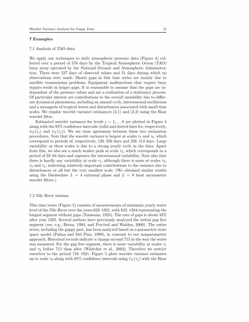
7.1 Analysis of TAO data

We apply our techniques to daily atmospheric pressure data (Figure 4) col-lected over a period of 578 days by the Tropical Atmospheric Ocean (TAO)buoy array operated by the National Oceanic and Atmospheric Administra-tion. There were 527 days of observed values and 51 days during which noobservations were made. Shorts gaps in this time series are mainly due tosatellite transmission problems. Equipment malfunctions that require buoyrepairs result in longer gaps. It is reasonable to assume that the gaps are in-dependent of the pressure values and are a realization of a stationary process.Of particular interest are contributions to the overall variability due to differ-ent dynamical phenomena, including an annual cycle, interseasonal oscillationsand a menagerie of tropical waves and disturbances associated with small timescales. We employ wavelet variance estimators (3.1) and (3.2) using the Haarwavelet filter.

Estimated wavelet variances for levels j = 1, . . . 8 are plotted in Figure 4along with the 95% confidence intervals (solid and dotted lines for, respectively,uX(τj) and vX(τj)). We see close agreement between these two estimationprocedures. Note that the wavelet variance is largest at scales τ7 and τ8, whichcorrespond to periods of, respectively, 128–256 days and 256–512 days. Largevariability at these scales is due to a strong yearly cycle in the data. Apartfrom this, we also see a much weaker peak at scale τ5, which corresponds to aperiod of 32–64 days and captures the interseasonal variability. Note also thatthere is hardly any variability at scale τ1, although there is some at scales τ2,τ3 and τ4, indicating relatively important contributions to the variance due todisturbances at all but the very smallest scale. (We obtained similar resultsusing the Daubechies L = 4 extremal phase and L = 8 least asymmetricwavelet filters.)

7.2 Nile River minima

This time series (Figure 5) consists of measurements of minimum yearly waterlevel of the Nile River over the years 622–1921, with 622–1284 representing thelongest segment without gaps (Toussoun, 1925). The rate of gaps is about 43%after year 1285. Several authors have previously analyzed the initial gap freesegment (see, e.g., Beran, 1994, and Percival and Walden, 2000). The entireseries, including the gappy part, has been analyzed based on a parametric statespace model (Palma and Del Pino, 1999), in contrast to our nonparametricapproach. Historical records indicate a change around 715 in the way the serieswas measured. For the gap free segment, there is more variability at scales τ1

and τ2 before 715 than after (Whitcher et al., 2002). Therefore we restrictourselves to the period 716–1921. Figure 5 plots wavelet variance estimatesup to scale τ8 along with 95% confidence intervals using vX(τj) with the Haar


wavelet filter. Here solid lines stand for the gap free segment 716–1284, anddotted lines for the gappy segment 1286–1921. Except at scales τ1, τ6 and τ8,we see reasonably good agreement between estimates from the two segments.Substantial uncertainties due to the large number of gaps are reflected in thelarger confidence intervals for the gappy segment. Under the assumption thatthe statistical properties of the Nile River were the same throughout 716–1921,we could combine the two segments to produce overall estimates and confidenceintervals for the wavelet variances; however, this assumption is questionableat certain scales. Over the years 1286–1470, there are only six gaps. Separateanalysis of this segment suggests more variability at scales τ1 and τ2 than whatwas observed in 716–1284. In addition, construction of the first Aswan Damstarting in 1899 changed the nature of the Nile River in the subsequent years.However, a wavelet variance analysis over 1286–1898 (omitting the years afterthe dam was built) does not differ much from that of 1286–1921. Thus theapparent increase in variability at the largest scales from segment 716–1284to 1286–1921 cannot be attributed just to the influence of the dam.

8 Discussion

In Section 3 we made the crucial assumption that, for a fixed j, β−1l,l′ > 0

when l, l′ = 0, . . . , Lj − 1. For small sample sizes, this condition might failto hold. This situation arises mainly when half or more of the observationsare missing and can be due to systematic periodic patterns in the gaps. Forexample, if δt alternates between zero and one, then β−1

0,1 is zero, reflectingthe fact that the observed time series does not contain relevant informationabout ν2

X(τ1). A methodology different from what we have discussed might be

able to handle some gap patterns for which β−1l,l′ = 0. In particular, generalized

prolate spheroidal sequences have been used to handle spectral estimation ofirregularly sampled processes (Bronez, 1988). This approach in essence cor-responds to the construction of special filters and could be used to constructapproximations to the Daubechies filters when β−1

l,l′ = 0.Estimation of the SDF for gappy time series is a long-standing difficult

problem. In Section 1 we noted that the wavelet variance provides a simpleand useful estimator of the integral of the SDF over a certain octave band. Inparticular, the Blackman–Tukey pilot spectrum (Blackman and Tukey, 1958,Sec. 18) coincides with the Haar wavelet variance. Recently Tsakiroglou andWalden (2002) generalized this pilot spectrum by utilising the (maximal over-lap) discrete wavelet packet transform. The result is an SDF estimator thatis competitive with existing estimators. With a similar generalization, ourwavelet variance estimator for gappy time series can be adapted to serve asan SDF estimator. Moreover, Nason et al. (2000) used shrinkage of squaredwavelet coefficients to estimate spectra for locally stationary processes. In thesame vein, we can apply wavelet shrinkage to the Zu,j,t or Zv,j,t processes toestimate time-varying spectra when the original time series is observed withgaps.


Finally we note a generalization of interest in the analysis of multivariategappy time series. Given two time series X1,t and X2,t, the wavelet crosscovariance yields a scale-based analysis of the cross covariance between thetwo series in a manner similar to wavelet variance analysis (for estimationof the wavelet cross covariance, see Whitcher et al., 2000, and the referencestherein). The methodology described in this paper can be readily adapted toestimate the wavelet cross covariance for multivariate time series with gaps.

A Proofs

We first need the followings propositions and lemmas. To avoid a triviality, we assumethroughout that var {Xt} > 0.

Proposition A.1 Let Xt be a real-valued zero mean Gaussian process with ACVS sX,k

and with SDF SX that is square integrable over [− 12, 12]. Then the bivariate process Ut ≡

ˆ

Xt−kXt−k′ ,Xt−lXt−l′˜T

, for any choice of k, k′, l and l′, has a spectral matrix SU thatis continuous.

Proof Using the Isserlis theorem, we have

cov“

Xt−kXt−k′ ,Xt−l+τXt−l′+τ

”

= sX,k−l+τsX,k′−l′+τ + sX,k−l′+τsX,k′−l+τ .

By the Fourier transform we obtain

Sk,k′,l,l′ (f) = ei2πf(k′−l′)Z 1/2

−1/2ei2πf ′(k−l−k′+l′)SX(f ′)SX(f − f ′) df ′

+ei2πf(k′−l)

Z 1/2

−1/2ei2πf ′(k+l−k′−l′)SX(f ′)SX(f − f ′) df ′.

Because exp{i2πf(k′ − l′)} is a continuous function of f , we can establish the continuity ofthe first term above if we can show that

Ak,k′,l,l′ (f) ≡

Z 1/2

−1/2ei2πf ′(k−l−k′+l′)SX(f ′)SX(f − f ′) df ′

is a continuous function, from which the continuity of the second term – and hence ofSk,k′,l,l′ itself – follows immediately. The Chauchy–Schwarz inequality says that

˛

˛Ak,k′,l,l′ (f + ρ) −Ak,k′,l,l′(f)˛

˛

=

˛

˛

˛

˛

˛

Z 1/2

−1/2ei2πf ′(k−l−k′+l′)SX(f ′)

ˆ

SX(f + ρ− f ′) − SX(f − f ′)˜

df ′

˛

˛

˛

˛

˛

≤

Z 1/2

−1/2S2

X(f ′) df ′Z 1/2

−1/2

˛

˛SX(f + ρ− f ′) − SX(f − f ′)˛

˛

2df ′

!1/2

.

By hypothesisR 1/2−1/2

S2X(f ′) df ′ is finite, while

Z 1/2

−1/2

˛

˛SX(f + ρ− f ′) − SX(f − f ′)˛

˛

2df ′ → 0 as ρ → 0

by Lemma 1.11, p. 37 of Zygmund (1978). Hence Ak,k′,l,l′ and Sk,k′,l,l′ are continuous. ⊓⊔


Proposition A.2 Let hj,l be any filter of finite width Lj with squared gain function Hj.Define Sk,k′,l,l′ as in Proposition A.1 in terms of a squared integrable SX . Then we musthave

X

k,k′

X

l,l′

hj,khj,k′hj,lhj,l′Sk,k′,l,l′(0) > 0.

Proof Using the definition of Sk,k′,l,l′ , it follows that

X

k,k′

X

l,l′

hj,khj,k′hj,lhj,l′Sk,k′,l,l′ (0) = 2

Z 1/2

−1/2H2

j (f ′)S2X(f ′) df ′,

which is strictly positive because Hj is zero only on a set of Lebesgue measure zero andvarXt > 0. ⊓⊔

Proposition A.3 Let Xt be a real-valued zero mean Gaussian process with ACVS sX,k

and SDF SX satisfyingZ 1/2

−1/2sin4(2πf)S2

X (f) df <∞.

Then the bivariate process Ut =ˆ

12(Xt−k −Xt−k′ )2, 1

2(Xt−l −Xt−l′)

2˜T

, for any choiceof k, k′, l and l′, has a spectral matrix SU that is continuous.

Proof The proof is similar to that of Proposition A.1. ⊓⊔

Proposition A.4 Let hj,l be as in Proposition A.2. Assume the conditions of Proposi-tion A.3, and let Sk,k′,l,l′ be the (k, k′, l, l′) component of SU in that proposition. Then

X

k,k′

X

l,l′


Proof The proof is similar to that of Proposition A.2. ⊓⊔

Lemma A.5 Let Ul,l′,t and Vl,l′,t be stationary processes that are independent of eachother for any choice of k, k′, l and l′. Let

Ul,l′,t = ψl,l′ +

Z 1/2

−1/2ei2πftdUl,l′ (f)

Vl,l′,t = ωl,l′ +

Z 1/2

−1/2ei2πftdVl,l′ (f)

be their respective spectral representations. For any k, k′, l and l′, let Sk,k′,l,l′ and Gk,k′,l,l′

denote the respective cross spectrum between Uk,k′,t and Ul,l′,t and between Vk,k′,t andVl,l′,t. Let al,l′ be fixed real numbers. Define

Qt =X

l,l′

al,l′ (Ul,l′,tVl,l′,t − ψl,l′ωl,l′ ).

Then Qt is a second order stationary process whose spectral density function is given by

SQ(f) ≡X

k,k′

X

l,l′

ak,k′al,l′ˆ

ψk,k′ψl,l′Gk,k′,l,l′(f) + ωk,k′ωl,l′Sk,k′,l,l′ (f)(A.1)

+ S ∗Gk,k′,l,l′(f)˜

,

where

S ∗Gk,k′,l,l′(f) ≡

Z 1/2

−1/2Gk,k′,l,l′(f − f ′)Sk,k′,l,l′ (f

′) df ′.


Proof A full proof is straightforward, but tedious. The key steps are to note that

cov {Qt, Qt+m} =X

k,k′,l,l′

ak,k′al,l′cov {Uk,k′,tVk,k′,t, Ul,l′,t+mVl,l′,t+m}, (A.2)

to use the spectral representations of Ul,l′,t and Vl,l′,t and the independence assumption toobtain

cov {Uk,k′,tVk,k′,t, Ul,l′,t+mVl,l′,t+m}

=

Z 1/2

−1/2ei2πfm

"

ψk,k′ψl,l′Gk,k′,l,l′(f) + ωk,k′ωl,l′Sk,k′,l,l′(f)

+

Z 1/2

−1/2Gk,k′,l,l′ (f − f ′)Sk,k′,l,l′(f

′) df ′

#

df,

and to plug the above formula into equation (A.2). ⊓⊔

Proposition A.6 Let Xt be a real-valued zero mean Gaussian stationary process withACVS sX,m and SDF SX that is square integrable over [− 1

2, 1

2]. Let δt be a binary-valued

strictly stationary process that is independent of Xt and satisfies Assumption 4.1. Let Zu,j,t

be as in equation (4.1). Then Zu,j,t is a second order stationary process whose SDF at zerois strictly positive.

Proof Let Ul,l′,t = Xt−lXt−l′ , Ut =ˆ

Uk,k′,t, Ul,l′,t

˜T, Vl,l′,t = δt−lδt−l′ and al,l′ =

hj,lhj,l′βl−l′ . By Proposition A.1, Ut has a continuous cross spectrum Sk,k′,l,l′ . Then byLemma A.5, the SDF Su,j(f) of Zu,j,t is given by the right-hand side of equation (A.2),

where ψl,l′ = EXt−lXt−l′ , ωl,l′ = E δt−lδt−l′ = β−1l−l′

and Gk,k′,l,l′ is the cross spectrum

between δt−kδt−k′ and δt−lδt−l′ . Since al,l′ωl,l′ = hj,lhj,l′ , by Proposition A.2

X

k,k′

X

l,l′

ak,k′al,l′ωk,k′ωl,l′Sk,k′,l,l′ (0) =X

k,k′

X

l,l′


NowP

k,k′

P

l,l′ ak,k′al,l′ψk,k′ψl,l′Gk,k′,l,l′ (f) andP

k,k′

P

l,l′ ak,k′al,l′S∗Gk,k′,l,l′ (f) arenonnegative because Gk,k′,l,l′ and Sk,k′,l,l′ are entries of spectral density matrices. HenceSu,j(0) > 0. ⊓⊔

Proposition A.7 Let Xt be a real-valued Gaussian stationary process with zero mean, andSDF SX that satisfies

Z 1/2

−1/2sin4(πf)S2

X (f) df < ∞.

Let δt be a binary-valued strictly stationary process that is independent of Xt and satisfiesAssumption 4.1. Let Zv,j,t be as in equation (4.2). Then Zv,j,t is a second order stationaryprocess whose SDF at zero is strictly positive.

Proof The proof closely parallels that of Proposition A.6. Here we take Ul,l′,t = − 12(Xt−l−

Xt−l′)2 and use Propositions A.3 and A.4 instead of Propositions A.1 and A.2. ⊓⊔

Next we state the following theorem from Brillinger (1981), p. 21.

Theorem A.8 Consider a two way array of random variables (RVs) Θi,j, j = 1, . . . , Ji

and i = 1, . . . , n. Consider the n RVs Υi =QJi

j=1 Θi,j for i = 1, . . . , n. Then the jointcumulant of Υ1, . . . , Υn is given by the formula

cum(Υ1, . . . , Υn) =X

χ

cum(Θi,j : (i, j) ∈ χ1) · · · cum(Θi,j : (i, j) ∈ χr)


where the summation is over all indecomposable partitions χ = χ1 ∪ · · · ∪ χr of the (notnecessarily rectangular) two way table

(1, 1) · · · (1, J1)...

...(n, 1) · · · (n, Jn).

(A.3)

Next we need the following lemmas.

Lemma A.9 Assume that Xt satisfies the conditions stated in Theorem 4.2. Let Up,t =Xt−lXt−l′ and EUp,t = ψp, where p = (l, l′). Then for n ≥ 3 and fixed p1, . . . , pn,

X

t1,...tn

|cum(Up1,t1 − ψp1, . . . , Upn,tn − ψpn )| = o(Mn/2), (A.4)

where each ti ranges from 0 to M − 1 (here and below M is shorthand for Mj in the maintext).

Proof Since a cumulant is invariant under the addition of constants,

cum(Up1,t1 − ψp1, . . . , Upn,tn − ψpn ) = cum(Up1,t1 , . . . , Upn,tn).

Consider the n× 2 table of RVs given by

Θ1,1 = Xt1−l1 Θ1,2 = Xt1−l′1

.

.....

Θn,1 = Xtn−ln Θn,2 = Xtn−l′n.

As Up,t is the product of the two Gaussian RVs in row p of the table, we invoke Theorem A.8to break up cum(Up1,t1 , . . . , Upn,tn). Moreover, because all cumulants of order r ≥ 3 are zerodue to Gaussianity, we can restrict ourselves to indecomposable partitions χ = χ1 ∪ · · ·∪χn

of the two way table (A.3) with J1 = · · · = Jm = 2 so that |χk| = 2 for all k. LetP

t1,...,tncum(Up1,t1 , . . . , Upn,tn ) ≡

P

χ IU,M(χ) with

IU,M (χ) =X

t1,...,tn

cum(Θi,j : (i, j) ∈ χ1) · · · cum(Θi,j : (i, j) ∈ χn).

Since n is fixed and the number of indecomposable partitions depends only on n, it thensuffices to show that IU,M (χ) = o(Mn/2) for any fixed χ. As χ is an indecomposablepartition, without loss of generality (WLOG), we can properly order the index of table(A.3) so that χk = {(k, ηk), (k + 1, ξk+1)} for k = 1, . . . , n − 1 and χn = {(n, ηn), (1, ξ1)},where ηk takes values of 1 or 2 for k = 1, . . . , n and ξk = 3 − ηk . We set, for k = 1, . . . , n,

ek =

8

>

>

>

>

<

>

>

>

>

:

l(k+1) mod n − lk , if ξ(k+1) mod n = ηk = 1

l′(k+1) mod n

− lk , if ξ(k+1) mod n = 2, ηk = 1

l(k+1) mod n − l′k , if ξ(k+1) mod n = 1, ηk = 2

l′(k+1) mod n

− l′k , if ξ(k+1) mod n = ηk = 2

Then we can writecum(Θi,j : (i, j) ∈ χk) = sX,tk+1−tk−ek

for k = 1, . . . , n− 1 and cum(Θi,j : (i, j) ∈ χn) = sX,t1−tn−en. Hence

IU,M(χ) ≡X

t1,...,tn

sX,t1−tn−en

n−1Y

i=1

sX,ti+1−ti−ei. (A.5)


For a fixed K, write IU,M (χ) = I′U,M(χ) + I′′U,M (χ), where I′U,M (χ) is the sum of (A.5)

taken over ti, i = 1, . . . , n, such that |ti+1 − ti| ≤ K for i = 1, . . . , n− 1 and |t1 − tn| ≤ K.Set qi = ti+1−ti for i = 1, . . . , n−1. Since sX,τ is bounded in magnitute by sX,0, we obtain

|I′U,M(χ)| ≤ sX,0

X

|qi|≤K, i=1,...,n−1

X

tn

1 ≤ sX,0Kn−1M.

The rest of the proof runs parallel to that of Lemma 6 of Giraitis and Surgailis (1985). Thuswe show that I′′U,M (χ) ≤ ǫ(K)Mn/2 where ǫ(K) → 0 as K → ∞. We repeatedely use theCauchy–Schwartz inequality to obain

I′′U,M(χ)

=X

t1,...,tn

sX,t1−tn−en

n−1Y

i=1

sX,ti+1−ti−ei

=X

t1,...,tn−1

n−2Y

i=1

sX,ti+1−ti−ei

X

tn

sX,t1−tn−ensX,tn−tn−1−en−1

≤X

t1,...,tn−1

n−2Y

i=1

sX,ti+1−ti−ei

“

X

tn

s2X,t1−tn−en

” 12“

X

tn

s2X,tn−tn−1−en−1

” 12

=X

t1,...,tn−2

n−3Y

i=1

sX,ti+1−ti−ei

“

X

tn

s2X,t1−tn−en

” 12X

tn−1

sX,tn−1−tn−2−en−2

“

X

tn


” 12

≤X

t1,...,tn−2

n−3Y

i=1

sX,ti+1−ti−ei

“

X

tn

s2X,t1−tn−en

” 12“

X

tn−1

s2X,tn−1−tn−2−en−2

” 12

“

X

tn−1,tn


” 12

..

.

≤“

X

t1,tn

s2X,t1−tn−en

” 12

nY

i=2

“

X

ti−1,ti

s2X,ti−ti−1−ei−1

” 12

Now use the fact that ti ranges from 0 to M − 1 and |ti+1 − ti| > K for i = 1, . . . , n− 1 and|t1 − tn| > K. Thus for example

X

ti−1,ti

s2X,ti−ti−1−ei−1≤ constant

X

|τ |>K

X

ti

s2X,τ = constant MX

|τ |>K

s2X,τ ,

whereP

|τ |>K s2X,τ goes to zero as K → ∞ because of the square integrability assumption.

Hence we have

I′′U,M(χ) ≤ constant M12

n“

X

|τ |>K

s2X,τ

” 12

n= ǫ(K)M

12

n,

and the required result follows by choosing K = ⌊log(M)⌋. ⊓⊔

Lemma A.10 Assume that Xt satisfies the conditions stated in Theorem 4.4. Let Up,t =− 1

2(Xt−l − Xt−l′)

2 and EUp,t = ψp, in which p = (l, l′). Then for n ≥ 3 and fixedp1, . . . , pn,

X

t1,...tn

|cum(Up1,t1 − ψp1, . . . , Upn,tn − ψpn )| = o(Mn/2),


where each ti ranges from 0 to M − 1.

Proof The proof goes as that of Lemma A.9 with the modification that Up,t can be written asthe product ofXt−l−Xt−l′ and − 1

2(Xt−l−Xt−l′), where the Gaussian process Xt−l−Xt−l′

has a squared integrable SDF. ⊓⊔

Lemma A.11 Let Up,t be either as in Lemma A.9 or as in Lemma A.10. Assume

κn(p1, . . . , pn, t1, . . . , tn) = cum(Up1,t1 − ψp1, . . . , Upn,tn − ψpn ).

Define for i = 1, 2, . . . , n− 1

κn(p1, . . . , pn, t1, . . . , ti) =X

ti+1,...,tn

M− 12(n−i−1)κn(p1, . . . , pn, t1, . . . , tn),

where the summation in tj ranges from 0 to M−1. Then κn(p1, . . . , pn, t1, . . . , ti) is boundedand satisfies

X

t1,...,ti

κn(p1, . . . , pn, t1, . . . , ti) = o“

M12(i+1)

”

, i = 1, 2, . . . , n. (A.6)

Proof We retain all the notation of Lemma A.9. Thus

κn(p1, . . . , pn, t1, . . . , tn) =X

χ

sX,t1−tn−en

n−1Y

i=1

sX,ti+1−ti−ei

Since equation (A.6) follows from (A.4), it suffices to show that for any fixed χ

X

tλ1,...,tλi

M− 12(i−1)sX,t1−tn−en

n−1Y

i=1

sX,ti+1−ti−ei(A.7)

is bounded for any distinct choice of λ1, . . . , λi that belong to {1, . . . , n} and i < n.Consider i = 1. WLOG assume λ1 = n. Then

X

tn

sX,t1−tn−en

n−1Y

i=1

sX,ti+1−ti−ei

≤

n−2Y

i=1

sX,ti+1−ti−ei

“

X

tn

s2X,t1−tn−en

” 12“

X

tn


” 12,

which is bounded because of the square integrability assumption. Thus (A.7) is bounded.Now consider i = 2. WLOG assume λ1 = n. Now we have two cases. In the first case

λ2 = 1 or n − 1 so that the pair tλ1, tλ2

appears together in a single term involving sX in(A.7). If we assume WLOG λ2 = n− 1 we obtain

X

tn−1,tn

M− 12 sX,t1−tn−en

n−1Y

i=1

sX,ti+1−ti−ei

≤X

tn−1

M− 12

n−2Y

i=1

sX,ti+1−ti−ei

“

X

tn

s2X,t1−tn−en

” 12“

X

tn


” 12

≤

n−3Y

i=1

sX,ti+1−ti−ei

“

X

tn

s2X,t1−tn−en

” 12“

X

tn−1


” 12

“

M−1X

tn−1,tn


” 12


Clearly the above expression is bounded becauseP

t s2X,t is so and therefore

limM→∞

M−1X

tn−1,tn

s2X,tn−tn−1−en−1=X

τ

s2X,τ−en−1<∞.

Thus (A.7) is bounded. In the second case assume λ2 = n− 2. Thus tλ1, tλ2

appear in twodistinct terms involving sX in (A.7). Hence

X

tn−2,tn

sX,t1−tn−en

n−1Y

i=1

sX,ti+1−ti−ei

≤X

tn−2

n−2Y

i=1

sX,ti+1−ti−ei

“

X

tn

s2X,t1−tn−en

” 12“

X

tn


” 12

≤

n−4Y

i=1

sX,ti+1−ti−ei

“

X

tn

s2X,t1−tn−en

” 12“

X

tn


” 12

“

X

tn−1


” 12“

X

tn−2


” 12

Clearly this is bounded. Note that we do not need to use the M− 12 factor. Thus boundedness

of (A.7) holds.The pattern for the general proof is now clear. Note that, because χ is an indecomposable

partition, there can be at most i − 1 pairs of λi, namely (λj , λj+1) for j = 1, . . . , i − 1such that each of (i − 1) pairs (tλj

, tλj+1) appears in distinct i − 1 terms involving sX

in the equation (A.7). Thus summing over tλjfor j = 1, . . . , i in the left hand side of

(A.7) and repeated use of Cauchy–Schwartz inequality will give rise to the (i − 1) termsM−1

P

tλj,tλj+1

s2X,tλj+1−tλj

−eλj

, j = 1, . . . , i− 1. Note that all these terms are bounded

and hence boundedness of (A.7) follows. Of course, if there are less than (i− 1) such pairs

(λj , λj+1), we no longer need to use the factor M− 12(i−1) (in fact in the exponent we just

need half the number of such pairs). This completes the proof. ⊓⊔

Proof (of Theorem 4.2) Take Up,t = Xt−lXt−l′ , Vp,t = δt−lδt−l′ and ap = hj,lhj,l′βl−l′ ,where p = (l, l′). Take Qt =

P

p ap(Up,tVp,t −ψpωp) as in Lemma A.5. Note that uX(τj)−

ν2X(τj) is the average of Qt over Lj − 1 ≤ t ≤ N − 1 with βl−l′ replaced by its consistent

estimate βl,l′ . Since Qt is stationary, we first prove a CLT for R = M− 12PM−1

t=0 Qt andthen invoke Slutsky’s theorem to complete the proof that uX(τj ) is asymptotically normal.We use Zurbenko (1986), p. 2, to write the log of the characteristic function of R as

logF (λ) =∞X

n=1

inλn

n!

X

t1,...,tn

Bn(t1, . . . , tn)

Mn/2,

where Bn is the nth order cumulant of Qt, and each ti ranges from 0 to M − 1. Since Qt

is centered, B1(t1) = 0. By Proposition A.6, the autocovariances sQ,τ of Qt are absolutelysummable and M−1

P

t1

P

t2B2(t1, t2) →

P

τ sQ,τ = SQ(0) > 0. In order to prove the

CLT for R, it suffices to show thatP

t1,...,tnM−n/2Bn(t1, . . . , tn) → 0 for n = 3, 4, . . ..

First using p. 19 of Brillinger (1981), we break up the nth order cumulant as follows:

Bn(t1, . . . , tn) =X

p1

· · ·X

pn

ap1· · · apn

cum(Up1,t1Vp1,t1 − ψp1ωp1

, . . . , Upn,tnVpn,tn − ψpnωpn ).


Let D1,p,t = (Up,t − ψp)(Vp,t − ωp), D2,p,t = ωp(Up,t − ψp) and D3,p,t = ψp(Vp,t − ωp).Then Up,tVp,t − ψpωp = D1,p,t +D2,p,t +D3,p,t. Using p. 19 of Brillinger (1981) again, wehave

cum(Up1,t1Vp1,t1 − ψp1ωp1

, . . . , Upn,tnVpn,tn − ψpnωpn )

=X

c1,...,cn

cum(Dc1,p1,t1 , . . . ,Dcn,pn,tn ),

where each ci ranges from 1 to 3. Therefore, it suffices to show that, for fixed p1, . . . , pn

and c1, . . . , cn, cum(Dc1,p1,t1 , . . . ,Dcn,pn,tn ) = o(Mn/2). Since the cumulant of n RVsis invariant under a reordering of the RVs, assume c1 = c2 = · · · = cm = 1, cm+1 =cm+2 = · · · = cm′ = 2, cm′+1 = cm′+2 = · · · = cn = 3, and consider a two way tableΘi,j with n rows. Rows i = 1, . . . ,m each contain exactly two RVs, namely, Upi,ti

− ψpi

and Vpi,ti− ωpi

(note that the product of the RVs in row i is D1,pi,ti). The remaining

n −m rows contain one RV each, namely, Upi,ti− ψpi

(which is proportional to D2,pi,ti)

for i = (m + 1), . . . ,m′, and Vpi,ti− ωpi

(proportional to D3,pi,ti) for i = m′ + 1, . . . , n.

Theorem 4 says cum(Dc1,p1,t1 , . . . ,Dcn,pn,tn ) is proportional toP

χ cum(Θi,j : (i, j) ∈

χ1) · · · cum(Θi,j : (i, j) ∈ χr). We complete the proof by showing that for any fixed χ

X

t1,...,tn

cum(Θi,j : (i, j) ∈ χ1) · · · cum(Θi,j : (i, j) ∈ χr) = o(Mn/2). (A.8)

We prove the above in the following steps.

step 1: Since Θi,j is centered, its first order cumulant is zero, so we can restrict ourselvesto cases where |χk| ≥ 2 for all k. If any group of RVs in Θi,j : (i, j) ∈ χk is independent ofthe remaining RVs in that set, then cum(Θi,j : (i, j) ∈ χk) = 0. Since the Upi,ti

−ψpi’s and

Vpi,ti−ωpi

’s are independent, we need only consider χk containing either just Upi,ti−ψpi

’sor just Vpi,ti

− ωpi’s.

step 2: Consider m = 0. In this case each row in Θi,j has only one RV, and thus allof Θi,j together form the only indecomposable partition χ = χ1. Now if m′ = 0, then byAssumption 4.1

X

t1,...,tn

cum(Θi,j : (i, j) ∈ χ)

=X

t1,...,tn

cum(Vp1,t1 − ωp1, . . . , Vpn,tn − ωpn ) = o(Mn/2).

On the other hand if m′ = n, then by Lemma A.9

X

t1,...,tn

cum(Θi,j : (i, j) ∈ χ)

=X

t1,...,tn

cum(Up1,t1 − ωp1, . . . , Upn,tn − ωpn ) = o(Mn/2).

Finally we rule out the case 1 ≤ m′ < n because then χ contains both Upi,ti− ψpi

’s andVpi,ti

− ωpi’s and hence cum(Θi,j : (i, j) ∈ χ) = 0.

step 3: Finally consider m ≥ 1. Assume that χ1, . . . , χq partition the random variables{Θ1,1, . . ., Θm′,1} (these are all Upi,ti

− ψpi) and that χq+1, . . . , χr partition the random

variables {Θ1,2, . . . , Θm,2, Θm′+1,1, . . . , Θn,1} (these are all Vpi,ti− ωpi

). To check that(A.8) holds, we need to consider five cases.

case 1: When m′ > m we sum over tm+1, . . . , tm′ in the left hand side of (A.8) anduse (A.6). In order to keep track of all the individual ti for which (i, 1) belongs to χk fork = 1, . . . , q, we set 0 = ρ0 ≤ ρ1 ≤ · · · ≤ ρq = m, m = σ0 ≤ σ1 ≤ · · · ≤ σq = m′ andassume, for k = 1, . . . , q, χk = {(ρk−1 + 1, 1), . . . , (ρk , 1), (σk−1 + 1, 1), . . . , (σk , 1)}. Then,


for k = 1, . . . , q, we obtain by Lemma A.11

X

tσk−1+1,...,tσk

cum(Θi,j : (i, j) ∈ χk)

=X

tσk−1+1,...,tσk

κρk+σk−ρk−1−σk−1(pi, ti : (i, 1) ∈ χk)

= M12(σk−σk−1−1)+κρk+σk−ρk−1−σk−1

(pi, : (i, 1) ∈ χk, tρk−1+1, . . . , tρk).

Now boundedness of κρk+σk−ρk−1−σk−1(pi, (i, 1) ∈ χk, tρk−1+1, . . . , tρk

) yields

M− 12(m′−m−1)

X

t1,...,tn


∝X

t1,...,tm

X

tm′+1,...,tn

cum(Θi,j : (i, j) ∈ χq+1) · · · cum(Θi,j : (i, j) ∈ χr) = o(M12

n).

The last equality follows from Assumption 4.1.

case 2: If m′ = m and |χk| > 2 for some k in q + 1, . . . , r, then using the boundednessof cum(Θi,j : (i, j) ∈ χk′) for k′ = 1, . . . , q, we obtain

X

t1,...,tn


≤ C0

X

t1,...,tn

cum(Θi,j : (i, j) ∈ χq+1) · · · cum(Θi,j : (i, j) ∈ χr) = o(Mn/2).

In the above C0 is a constant and the last equality follows from Assumption 4.1.

case 3: Consider |χk| = 2 for k = q+1, . . . , r and assume m′ = m. Clearly 2m > n > m

and r − q = n − m. Let (m + i, 1) be contained in χq+i for i = 1, . . . , n. We sum overtm+1, . . . , tn to obtain

X

t1,...,tn


≤ constantX

t1,...,tm

cum(Θi,j : (i, j) ∈ χ1) · · · cum(Θi,j : (i, j) ∈ χq)

cum(Θi,j : (i, j) ∈ χq+n−m+1) · · · cum(Θi,j : (i, j) ∈ χr)

≤ constantX

t1,...,tm

cum(Θi,j : (i, j) ∈ χ1) · · · cum(Θi,j : (i, j) ∈ χq) = o(M12

n).

In the above derivation we need the fact thatP

ticum(Vpi,ti

, Vpτ ,tτ ) is bounded and notethat the constant is changing from line to line.

case 4: Consider the case n = m. Again if any |χk| > 2 for k = 1, . . . , q, we are done byusing (A.4) along with the fact that cumulants of Vpi,ti

− ωpiare bounded.

case 5: The last case is n = m and |χk| = 2 for all k. The proof requires Theorem 4to write down the left hand side of (A.8) in terms of covariances of Upi,ti

and Vpi,tiand

hinges on the fact that ACVS of Upi,tiand Vpi,ti

are absolutely summable. ⊓⊔

Proof of Theorem 4.4. Take Up,t = − 12(Xt−l − Xt−l′)

2, Vp,t = δt−lδt−l′ and ap =hj,lhj,l′βl−l′ , where p = (l, l′). Use Lemma 3 in place of Lemma 2 and complete the proofas in Theorem 4.2 by checking all the steps. ⊓⊔

Acknowledgements We thank Peter Guttorp and Chris Bretherton for discussions.


References

Beran, J. (1994). Statistics for long-memory processes. New York: Chapman and Hall.Blackman, R. B., Tukey, J. W. (1958). The measurement of power spectra. New York: Dover

Publications.Breuer, P., Major, P. (1983). Central limit theorems for nonlinear functionals of Gaussian

fields. Journal of Multivariate Analysis 13, 425–441.Brillinger, D. R. (1981). Time series. Oakland, CA: Holden-Day Inc.Bronez, T. P. (1988). Spectral estimation of irregularly sampled multidimensional processes

by genelarized prolate spheroidal sequences. IEEE Transactions on Acoustics, Speech,and Signal Processing 36, 1862–1873.

Candes, E. J., Donoho, D. L. (2002). Recovering edges in ill-posed inverse problems: opti-mality of curvelet frames. The Annals of Statistics 30, 784–842.

Chiann, C., Morettin, P. A. (1998). A wavelet analysis for time series. Nonparametric Statis-tics 10, 1–46.

Craigmile, P. F., Percival, D. B. (2005). Asymptotic decorrelation of between-scale waveletcoefficients. IEEE Transactions on Information Theory 51, 1039–1048.

Daubechies, I. (1992). Ten lectures on wavelets. Philadelphia: SIAM.Donoho, D. L., Johnstone, I. M. (1998). Minimax estimation via wavelet shrinkage. The

Annals of Statistics 26, 879–921.Donoho, D. L., Johnstone, I. M., Kerkyacharian, G., Picard, D. (1995). Wavelet shrinkage:

asymptopia? Journal of the Royal Statistical Society. Series B. Methodological 57, 301–369.

Foster, G. (1996). Wavelets for period analysis of unevenly sampled time series. The Astro-nomical Journal 112, 1709–1729.

Fox, R., Taqqu, M. S. (1987). Central limit theorems for quadratic forms in random variableshaving long-range dependence. Probability Theory and Related Fields 74, 213–240.

Frick P., Grossmann, A., Tchamitchian P. (1998). Wavelet analysis of signals with gaps.Journal of Mathematical Physics 39, 4091–4107.

Genovese, C. R., Wasserman, L. (2005). Confidence sets for nonparametric wavelet regres-sion. The Annals of Statistics 33, 698–729.

Giraitis, L., Surgailis, D. (1985). CLT and other limit theorems for functionals of Gaussianprocesses. Zeitschrift fur Wahrscheinlichkeitstheorie und Verwandte Gebiete 70, 191–212.

Giraitis, L., Taqqu, M. S. (1998). Central limit theorems for quadratic forms with time-domain conditions. The Annals of Probability 26, 377–398.

Granger, C. W. J., Joyeux, R. (1980). An introduction to long-memory time series modelsand fractional differencing. Journal of Time Series Analysis 1, 15–29.

Greenhall, C. A., Howe, D. A., Percival, D. B. (1999). Total variance, an estimator oflong-term frequency stability. IEEE Transactions on Ultrasonics, Ferroelectrics, andFrequency Control 46, 1183–1191.

Hall, P., Penev, S. (2004). Wavelet-based estimation with multiple sampling rates. TheAnnals of Statistics 32, 1933–1956.

Ho, H. C., Sun, T. C. (1987). A central limit theorem for noninstantaneous filters of astationary Gaussian process. Journal of Multivariate Analysis 22, 144–155.

Hosking, J. R. M. (1981). Fractional differencing. Biometrika 68, 165–176.Kalifa, J., Mallat, S. (2003). Thresholding estimators for linear inverse problems and decon-

volutions. The Annals of Statistics 31, 58–109.Labat, D., Ababou, R., Mangin, A. (2001). Introduction of wavelet analyses to rain-

fall/runoffs relationship for a karstic basin: the case of licq–atherey karstic system(France). Ground Water 39, 605–615.

Lark, R. M., Webster, R. (2001). Changes in variance and correlation of soil propertieswith scale and location: analysis using an adapted maximal overlap discrete wavelettransform. European Journal of Soil Science 52, 547–562.

Massel, S. R. (2001). Wavelet analysis for processing of ocean surface wave records. OceanEngineering 28, 957–987.


Nason, G. P., von Sachs, R., Kroisandt, G. (2000). Wavelet processes and adaptive estimationof the evolutionary wavelet spectrum. Journal of the Royal Statistical Society. SeriesB. Methodological 62, 271–292.

Neumann, M. H., von Sachs, R. (1997). Wavelet thresholding in anisotropic function classesand application to adaptive estimation of evolutionary spectra. The Annals of Statistics25, 38–76.

Palma, W., Del Pino, G. (1999). Statistical analysis of incomplete long-range dependentdata. Biometrika 86, 965–972.

Pelgrum, H., Schmugge, T., Rango, A., Ritchie, J., Kustas, B. (2000). Length-scale analysisof surface albedo, temperature, and normalized difference vegetation index in desertgrassland. Water Resources Research 36, 1757–1766.

Percival, D. B. (1995). On estimation of the wavelet variance. Biometrika 82, 619–631.Percival, D. B., Walden, A. T. (2000). Wavelet methods for time series analysis. Cambridge,

UK: Cambridge University Press.Pichot, V., Gaspoz, J. M., Molliex, S., Antoniadis, A., Busso, T., Roche, F., Costes, F.,

Quintin, L., Lacour, J. R., Barthelemy, J. C. (1999). Wavelet transform to quantify heartrate variability and to assess its instantaneous changes. Journal of Applied Physiology86, 1081–1091.

Rybak, J., Dorotovic, I. (2002). Temporal variability of the coronal green-line index (1947–1998). Solar Physics 205, 177–187.

Serroukh, A., Walden, A. T., Percival, D. B. (2000). Statistical properties and uses of thewavelet variance estimator for the scale analysis of time series. Journal of the AmericanStatistical Association 95, 184–196.

Stoica, P., Larsson, E. G., Li, J. (2000). Adaptive filter-bank approack to restoration andspectral analysis of gapped data. The Astronomical Journal 163, 2163–2173.

Sweldens, W. (1997). The lifting scheme: a construction of second generation wavelets. SIAMJournal on Mathematical Analysis 19, 511–546.

Torrence, C., Compo, G. P. (1998). A practical guide to wavelet analysis. Bulletin of theAmerican Meteorological Society 79, 61–78.

Toussoun, O. (1925). Memoire sur l’histoire du Nil. Memoires a l’Institut d’Egypte 9, 366–404.

Tsakiroglou, E., Walden, A. T. (2002). From Blackman–Tukey pilot estimators to waveletpacket estimators: a modern perspective on an old spectrum estimation idea. SignalProcessing 82, 1425–1441.

Vio, R., Strohmer, T., Wamsteker, W. (2000). On the reconstruction of irregularly sampledtime series. Publications of the Astronomical Society of the Pacific 112, 74–90.

Whitcher, B. J, Guttorp, P., Percival, D. B. (2000). Wavelet analysis of covariance withapplication to atmospheric time series. Journal of Geophysical Research 105, 14,941–14,962.

Whitcher, B. J, Byers, S. D., Guttorp, P., Percival, D. B. (2002). Testing for homogeneityof variance in time series: long memory, wavelets and the Nile river. Water ResourcesResearch 38, 1054–1070.

Zurbenko, I. G. (1986). The spectral analysis of time series. Amsterdam: North–Holland.Zygmund, A. (1978). Trigonometric series. Cambridge, UK: Cambridge University Press.


Table A.1 Summary of Monte Carlo results for AR(1) process

j

1 2 3 4 5 6

ν2X(τj ) 0.0500 0.0689 0.1079 0.1585 0.1907 0.1710

mean of uX,r(τj) 0.0502 0.0690 0.1084 0.1593 0.1911 0.1716

mean of vX,r(τj ) 0.0503 0.0692 0.1085 0.1592 0.1910 0.1715

M− 1

2

j S12

u,j(0) 0.0087 0.0057 0.0104 0.0230 0.0347 0.0429

s.d. of uX,r(τj) 0.0076 0.0055 0.0101 0.0204 0.0338 0.0431

mean of M− 1

2

j S12

u,j,r(0) 0.0071 0.0047 0.0086 0.0175 0.0288 0.0340

M− 1

2

j S12

v,j(0) 0.0027 0.0047 0.0102 0.0207 0.0345 0.0428

s.d. of vX,r(τj ) 0.0025 0.0044 0.0099 0.0205 0.0337 0.0428

mean of M− 1

2

j S12

v,j,r(0) 0.0022 0.0039 0.0085 0.0173 0.0285 0.0339

Table A.2 Summary of Monte Carlo results for FD( 56) process

j

1 2 3 4 5 6

ν2X(τj ) 0.2594 0.3078 0.4427 0.6831 1.0762 1.7050

mean of vX,r(τj ) 0.2599 0.3081 0.4421 0.6832 1.0771 1.7179

M− 1

2

j S12

v,j(0) 0.0141 0.0203 0.0399 0.0857 0.1899 0.4281

s.d. of vX,r(τj ) 0.0129 0.0186 0.0386 0.0847 0.1877 0.4275

mean of M− 1

2

j S12

v,j,r(0) 0.0119 0.0168 0.0330 0.0704 0.1567 0.3489


−1.0 −0.5 0.0 0.5 1.0

1.0

1.5

2.0

2.5

3.0

φ

Sv.

3(0)

Su.

3(0)

0.0 0.1 0.2 0.3 0.4 0.5

0.85

0.90

0.95

1.00

1.05

1.10

αS

v.3(0

)S

u.3(0

)

Fig. A.1 Plot of asymptotic efficiency of uX(τ3) with respect to vX (τ3) under autoregres-sive (left) and fractionally differenced (right) models.

0 200 400 600 800 1000

−3

−2

−1

01

2

time

obse

rved

ser

ies

1 2 3 4 5 6

0.05

0.10

0.15

0.20

0.25

0.30

j

wav

elet

var

ianc

e

Fig. A.2 Plot of a typical simulated gappy AR(1) time series and wavelet variances atvarious scales.


0 200 400 600 800 1000

−20

−15

−10

−5

05

time

obse

rved

ser

ies

1 2 3 4 5 6

0.5

1.0

1.5

2.0

2.5

jw

avel

et v

aria

nce

Fig. A.3 Plot of a typical simulated gappy FD( 56) time series and wavelet variances at

various scales. Solid lines indicate the estimated intervals while dotted lines indicate thetrue intervals.

0 100 200 300 400 500 600

1006

1008

1010

1012

1014

1016

time

obse

rved

ser

ies

1 2 3 4 5 6 7 8

0.2

0.4

0.6

0.8

1.0

1.2

j

wav

elet

var

ianc

e

Fig. A.4 Atmospheric pressure data (left) from NOAA’s TAO buoy array and Haar waveletvariance estimates (right) for scales indexed by j = 1, . . . , 8.


600 800 1000 1200 1400 1600 1800

910

1112

1314

15

year

Nile

Riv

er m

inim

a

1 2 3 4 5 6 7 8

0.00

0.10

0.20

0.30

jw

avel

et v

aria

nce

Fig. A.5 Nile River minima (left) and Haar wavelet variance estimates (right) for scalesindexed by j = 1, . . . , 8.

wavelet variance analysis for gappy time series - university of

Documents