weather-adjusting economic data - brookings institution · weather-adjusting economic data ......

227

MICHAEL BOLDINFederal Reserve Bank of Philadelphia

JONATHAN H. WRIGHTJohns Hopkins University

Weather-Adjusting Economic Data

ABSTRACT This paper proposes and implements a statistical methodol-ogy for adjusting employment data for the effects of deviations in weather from seasonal norms. This is distinct from seasonal adjustment, which controls only for the normal variation in weather across the year. We simultaneously control for both of these effects by integrating a weather adjustment step in the seasonal adjustment process. We use several indicators of weather, includ-ing temperature and snowfall. We find that weather effects can be important, shifting the monthly payroll change number by more than 100,000 in either direction. The effects are largest in the winter and early spring months and in the construction sector. A similar methodology is constructed and applied to data in the national income and product accounts (NIPA), although the manner in which NIPA data are reported makes it impossible to integrate weather and seasonal adjustments fully.

Macroeconomic time series are affected by the weather. In the first quarter of 2014, real GDP contracted by 0.9 percent at an annual-

ized rate. Commentators and Federal Reserve officials attributed part of the decline to an unusually cold winter and large snowstorms that hit the East Coast and the South during the quarter (Macroeconomic Advisers 2014; Yellen 2014).1 Similarly, the slowdown in growth in the first quarter of 2015 was widely ascribed to another exceptionally harsh winter and other transitory factors (Yellen 2015). While the effects of regular variation in

1. In November 2013, the Survey of Professional Forecasters expected a seasonally adjusted increase of 2.5 percent in 2014Q1. The original report for the quarter was 0.1 per-cent, later revised to -2.1 percent, and subsequently revised to -0.9 in the 2015 annual NIPA adjustments that included revisions to the seasonal adjustment process, as discussed in section III below. With a snapback rate of 4.6 percent in the second quarter, it is highly plausible that weather played a significant role in the decline.

228 Brookings Papers on Economic Activity, Fall 2015

weather within a year should, in principle, be taken care of by the seasonal adjustment procedures that are typically applied to economic data, these adjustments are explicitly not supposed to adjust for variations that are driven by deviations from the weather norms for a particular time of year. It is typically cold in February, depressing activity in some sectors, and sea-sonal adjustment controls for this. But seasonal adjustment does not control for whether a particular February is colder or milder than normal.

Our objective in this paper is to construct and implement a methodol-ogy for estimating how the data would have appeared if weather patterns had followed their seasonal norms. Monetary policymakers view weather effects as transitory—given the long and variable lags in monetary policy, policymakers do not generally seek to respond to weather-related factors. It follows from this that the economic indicators they are provided with ought, as far as possible, to be purged of weather effects. Moreover, we argue that failing to control for abnormal weather effects distorts conven-tional seasonal adjustment procedures.

The measurement of inflation provides a useful analogy. The Federal Reserve focuses on core inflation, excluding food and energy, rather than headline inflation. The motivation is not that food and energy are inherently less important expenditures but that fluctuations in their inflation rates are transitory. Core inflation is more persistent and forecastable, and indeed a forecast of core inflation may be the best way of predicting overall inflation (Faust and Wright 2013). In the same way, economic fluctuations caused by the weather are real, but they are transitory. We may obtain a better mea-sure of the economy’s underlying momentum by removing the effects of abnormal weather.

Economists have studied the effects of the weather on agricultural out-put for a long time, going back to the work of R. A. Fisher (1925). More recently, they have also used weather as an instrumental variable (see, for example, Miguel, Satyanath, and Serengeti [2004]), arguing that weather can be thought of as an exogenous driver of economic activity. Statis tical agencies sometimes judgmentally adjust extreme observations due to spe-cific weather events before applying their seasonal adjustment procedures.2 Although there is a long literature on seasonal adjustment, we are aware of only a few papers on estimating the effect of unseasonal weather on

2. Even when agencies do this, their goal is just to prevent the anomalous weather from distorting seasonals, not to actually adjust the data for the effects of the weather. We discuss this in more detail later.

MICHAEL BOLDIN and JONATHAN H. WRIGHT 229

macro economic aggregates. The few papers on the topic include those by Macroeconomic Advisers (2014), which regresses seasonally adjusted aggregate GDP on snowfall totals, estimating that snow reduced 2014Q1 GDP by 1.4 percentage points at an annualized rate; by Justin Bloesch and François Gourio (2014), who likewise study the relationship between weather and seasonally adjusted data; by Melissa Dell, Benjamin Jones, and Benjamin Olken (2012), who implement a cross-country study of the effects of annual temperature on annual GDP; and by Christopher Foote (2015), who studies weather effects on state-level employment data. None of these papers integrates weather adjustment into the seasonal adjustment process, however. This is what the current paper attempts to do.

We focus mainly, but not exclusively, on the seasonal adjustment of the Bureau of Labor Statistics (BLS) Current Employment Statistics (CES) survey (the “establishment” survey), which includes total nonfarm payrolls. We do so because it is clearly the most widely followed monthly economic indicator, and also because it is an indicator for which researchers can approximately replicate the official seasonal adjustment process, unlike the NIPA data. We consider simultaneously adjusting these data for both seasonal effects and unseasonal weather effects. This can be quite differ-ent from ordinary seasonal adjustment, especially during the winter and early spring. Month-over-month changes in nonfarm payrolls are in several cases higher or lower by as much as 100,000 jobs when using the proposed seasonal-and-weather adjustment rather than ordinary seasonal adjustment. Using seasonal-and-weather adjustment increases the estimated pace of employment growth in the winters of 2013–14 and 2014–15.

The plan for the remainder of this paper is as follows. In section I, we discuss alternative measures of unusual weather and evaluate how they relate to aggregate employment. This is intended to give us guidance on which weather indicators have an important impact on employment data. In section II, we describe seasonal adjustment in the CES and discuss how adjustment for unusual weather effects may be added into this—seasonal adjustment is implemented at the disaggregate level. In section III we extend the analysis to NIPA data. Section IV concludes.

I. Measuring Unusual Weather and Its Effect on Aggregate Employment Data

We need to construct measures of unseasonal weather that are suitable for adjusting the CES survey. We first obtained data from the National Centers for Environmental Information on daily maximum temperatures,


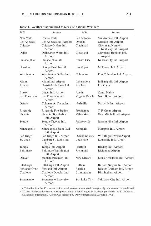
precipitation, snowfall, and heating degree days (HDDs)3 at one station in each of the largest 50 metropolitan statistical areas (MSAs) by population, in the United States from 1960 to the present. The stations were chosen to provide a long and complete history of data,4 and are listed in table 1. We averaged these across the 50 MSAs, with the averages weighted by population, determined from the 2010 census. This was designed as a way of measuring U.S.-wide temperature, precipitation, and snowfall in a way that makes a long time series easily available and that puts the highest weight on areas with the greatest economic activity. Weather, of course, varies substantially around the country, and it might seem more natural to adjust state-level employment data for state-level weather effects. We used national-level employment data with national-level weather because the BLS produces state and national data separately using different methodolo-gies. National CES numbers are quite different from the “sum of states” numbers, because both state and national CES numbers are constructed by survey methods, whereas the national data use more disaggregated cells. Meanwhile, it is the national numbers that garner virtually all the attention from Wall Street and the Federal Reserve.

Let temps denote the actual average temperature on day s, and define

the unusual temperature for the day as temp temp temps s s yy* 1

30,1

30∑= -=

, where

temps,y denotes the temperature on the same day y years previously. Like-wise, let prp*

s , snow*s , and hdd*

s denote the unusual precipitation, snowfall, or HDD on day s, relative to the 30-year average. This is in line with the meteorological convention of defining climate norms from 30-year aver-ages (World Meteorological Organization 2011).

In assessing the effect of unusual weather on employment as measured in the CES, we want to take careful account of the within-month timing of the CES survey. The CES survey relates to the pay period that includes the 12th day of the month. Some employers use weekly pay periods, others use biweekly periods, and a few use monthly periods. A worker is counted if she works at any point in that pay period. Cold weather or snow seems

3. The HDD at a given station on a given day is defined as max (18.3 - t, 0), where t is the average of maximum and minimum temperatures in degrees Celsius.

4. An alternative measure of snowfall, used by Macroeconomic Advisers (2014), is based on a data set of daily county-level snowfall maintained by the National Centers for Environmental Information. This clearly has the advantage of greater cross-sectional granu-larity. However, these data only go back to 2005. Our data go much further back, allowing us to construct a longer history of snowfall effects and to measure normal snowfall from 30-year averages.


Table 1. Weather Stations Used to Measure National Weather a

MSA Station MSA Station

New York Central Park San Antonio San Antonio Intl. AirportLos Angeles Los Angeles Intl. Airport Orlando Orlando Intl. AirportChicago Chicago O’Hare Intl.

AirportCincinnati Cincinnati/Northern

Kentucky Intl. AirportDallas Dallas/Fort Worth Intl.

AirportCleveland Cleveland Hopkins Intl.

AirportPhiladelphia Philadelphia Intl.

AirportKansas City Kansas City Intl. Airport

Houston George Bush Intcntl. Airport

Las Vegas McCarran Intl. Airport

Washington Washington Dulles Intl. Airport

Columbus Port Columbus Intl. Airport

Miami Miami Intl. Airport Indianapolis Indianapolis Intl. AirportAtlanta Hartsfield-Jackson Intl.

AirportSan Jose Los Gatos

Boston Logan Intl. Airport Austin Camp MabrySan Francisco San Francisco Intl.

AirportVirginia Beach Norfolk Intl. Airport

Detroit Coleman A. Young Intl. Airport

Nashville Nashville Intl. Airport

Riverside Riverside Fire Station Providence T. F. Green AirportPhoenix Phoenix Sky Harbor

Intl. AirportMilwaukee Gen. Mitchell Intl. Airport

Seattle Seattle-Tacoma Intl. Airport

Jacksonville Jacksonville Intl. Airport

Minneapolis Minneapolis-Saint Paul Intl. Airport

Memphis Memphis Intl. Airport

San Diego San Diego Intl. Airport Oklahoma City Will Rogers World AirportSt. Louis Lambert-St. Louis Intl.

AirportLouisville Louisville Intl. Airport

Tampa Tampa Intl. Airport Hartford Bradley Intl. AirportBaltimore Baltimore/Washington

Intl. AirportRichmond Richmond Airport

Denver Stapleton/Denver Intl. Airportb

New Orleans Louis Armstrong Intl. Airport

Pittsburgh Pittsburgh Intl. Airport Buffalo Buffalo Niagara Intl. AirportPortland (Ore.) Portland Intl. Airport Raleigh Raleigh-Durham Intl. AirportCharlotte Charlotte Douglas Intl.

AirportBirmingham Birmingham Airport

Sacramento Sacramento Executive Airport

Salt Lake City Salt Lake City Intl. Airport

a. This table lists the 50 weather stations used to construct national average daily temperature, snowfall, and HDD data. Each weather station corresponds to one of the 50 largest MSAs by population in the 2010 Census.

b. Stapleton International Airport was replaced by Denver International Airport in 1995.


most likely to affect employment status on the day of that unusual weather, but it is also possible that, for example, heavy snow might affect eco-nomic activity for several days after a snowstorm has ceased. Putting all this together, temperature/snowfall conditions in the days up to and including the 12th day of the month are likely to have some effect on measured employment for that month. The further before the 12th day of the month the unusual weather occurred, the less likely it is to have affected a worker’s employment status in the pay period bracketing the 12th, and so the less important it should be. It is hard to know a priori how to weight unusual weather on different days up to and including the 12th day of the month, but, on the other hand, it seems likely that unusual weather after the 12th day of the month ought to have little effect on employment data for that month.5

In solving this problem, we try to let the data speak. Our proposed approach assumes that the relevant temperature/precipitation/snowfall conditions are a weighted average of the temperature/precipitation/snowfall in the 30 days up to and including the 12th day of the month, using a Mixed Data Sampling (MIDAS) polynomial as the weights to avoid overfitting. We want to use this specification to collapse the daily weather data that we have into monthly weather measures. We will spell out the details of the MIDAS polynomial and its estimation below. MIDAS polynomials were proposed by Eric Ghysels, Pedro Santa-Clara, and Rossen Valkanov (2004, 2005) and by Elena Andreou, Ghysels, and Andros Kourtellos (2010) as a device for handling mixed frequency data in a way that is parsimonious yet flexible—exactly the problem that we face here. The presumption is that unusual weather on or just before the 12th day of the month should get more weight than unusual weather well before this date.

In addition to temperature, precipitation, snowfall, and HDDs, there are two other weather indicators that we consider. First, as an alternative way of measuring snowfall, the National Centers for Environmental Informa-tion produce regional snowfall indexes that measure the disruptive impact of significant snowstorms. These indexes take into account the area affected by the storm and the population in that area, for six different regions of the

5. There are actually ways in which weather after the 12th could matter for CES employ-ment that month. For example, suppose that a new hire was planning to begin work on the 13th and the 13th happens to be the last day of the pay period. She would be counted as employed in that month. But if bad weather caused the worker’s start date to be delayed, then she would not be defined as employed in that month. However, we do evaluate the possibility that weather just after the 12th could affect employment for that month.


country. See Paul Kocin and Louis Uccellini (2004) and Michael Squires and others (2014) for a discussion of these regional snowfall impact (RSI) indexes. They are designed to measure the societal impacts of different storms, which make them potentially very useful for our purposes. They have the drawback that they do not cover the western part of the country, but there are only two big cities that are not covered and that receive sig-nificant snowfall: Denver and Salt Lake City.

Any snowstorm affecting a region has an index value, a start date, and an end date. We treat the level of snowfall in that region as being equal to the index value from the start to the end date, inclusive. For example, a storm affecting the southeast region was rated as 10.666, started on Febru-ary 10, 2014, and ended on February 13, 2014. We treat this index as hav-ing a value of 10.666 on each day from February 10 to 13, 2014. For each of those days, we then create a weighted sum of the six regional snowstorm indexes to get a national value, where the weights are the populations in the regions (from the 2010 Census). We then used this RSI index as an alterna-tive to the average snowfall. Second, the household Current Population Survey (CPS) asks respondents if they were unable to work because of the weather. We seasonally adjust the number who were absent from work6 in month t, using the default X-13 filter, and then treat this variable, abst, as an additional weather indicator.

We first estimate eight candidate models giving the effects of differ-ent weather measures on aggregate employment. Intuitively, we are simply interested in regressing monthly aggregate not seasonally adjusted (NSA) employment onto a weighted average of daily weather data, where the weights give the best possible fit. This is intended as a precursor to incor-porating weather effects in CES seasonal adjustment. However, weather is only a very small part of what drives aggregate employment. We also want the model to allow for trend and seasonal components.

I.A. Eight Candidate Models

Each of our eight candidate models is an “airline model”—the default model in the first stage of the X-13—fitted to aggregate NSA employment, but augmented by weather variables. Each model specifies that there are trend and seasonal components that are nonstationary and consequently require taking first differences and differences from the same month one

6. This is the number with a job, not at work, in nonagricultural industries (series LNU02036012).


year earlier. After this differencing, the employment data are driven by weather effects and by moving average errors. The specific model is of the form

L L y x L Lt t t( )( ) ( )( ) ( )( )- - - ′g = + q + Q e1 1 1 1 1 ,12 12

where yt is total NSA employment for month t, L is the lag operator, and et is an independent and identically distributed error term. The eight models differ only in the specification of the regressors in xt. The specifications that we consider are as follows:

SPECIFICATION 1: TEMPERATURE ONLY There are 12 elements in xt, each of

which is ∑ -=w tempj s jj

*0

30 interacted with one of 12 monthly dummies, where

day s is the 12th day of month t, and where

w Bj

a bj30

, ,=

and

B x a bax bx

aj

bj

j∑ ( )

( ) ( )= +

+

=

; ,exp

exp30 30

.2

2

0

30

B(x; a, b) is the MIDAS polynomial. In all, this model has 17 parameters: the 12 elements of g along with a, b, q, Q, and the variance of the error term. Temperature is interacted with month dummies. The motivation for this is that the effect of temperature on the economy depends heavily on the time of year. For example, unusually cold weather in winter lowers building activity, but unusually cold weather in the summer might have little effect on this sector, or might even boost it. Likewise, warm weather boosts demand for electricity in summer but weakens demand for electric-ity in winter.

SPECIFICATION 2: HDD ONLY There are 12 elements in xt, each of which

is ∑ -=w hddj s jj

*0


( )=w Bj

a bj30

, , .

SPECIFICATION 3: TEMPERATURE AND SNOWFALL There are 13 elements in xt. The first 12 are as in specification 1. The 13th element is w snowj s jj∑ -=

*0

30,


where snow*s denotes the unusual snowfall on the 12th day of month t,

measured as the population-weighted average across the 50 MSAs. The monthly snow variable is not interacted with month dummies, because it falls only in the winter months, and its effect on employment is likely to be similar in any winter month.

SPECIFICATION 4: TEMPERATURE AND SNOWFALL (RSI INDEX) The specifi-cation is as in specification 3, except using the RSI index to measure snowfall.

SPECIFICATION 5: TEMPERATURE, SNOWFALL (RSI INDEX), AND WEATHER-RELATED

ABSENCES FROM WORK The specification is the same as in specification 4 except that abst is included in the 14th element of xt.

SPECIFICATION 6: TEMPERATURE, SNOWFALL (RSI INDEX), AND PRECIPITATION There are 14 elements in xt. The first 13 are as in specification 4. The 14th

element is w prpj s jj∑ -=*

0

30, where prp*

s denotes the unusual precipitation on

the 12th day of month t, measured as the population-weighted average across MSAs.

SPECIFICATION 7: TEMPERATURE, SNOWFALL (RSI INDEX), AND LAGS OF

TEMPERATURE AND SNOWFALL There are 13 elements in xt. Each of the first

12 is w tempj s jj∑ -=*

0


w Bj

a bj30

, ,=

for j ≤ 30, wj = c for 31 ≤ j ≤ 60, and wj = d for j > 60. The

last element is w snowj s jj∑ -=* .

0

90 In this specification, the parameters c and d

determine the weight of weather two and three months prior.SPECIFICATION 8: TEMPERATURE, SNOWFALL (RSI INDEX), AND TEMPERATURE

AND SNOWFALL JUST AFTER THE CES SURVEY DATE There are 13 elements in xt.

Each of the first 12 is w tempj s jj∑ -=-*

2

90 interacted with one of 12 monthly

dummies, where w Bj

a bj ( )=30

, , for j ≥ 0 and wj = c otherwise. The last

element is w snowj s jj∑ +=-* .

2

90 In this specification, we use a MIDAS-weighted

average of the days up to and including the 12th, and an extra parameter c determines the weight of weather on the 13th and 14th of the month.

Note that in all these specifications, we are assuming that the effect is linear in weather; unusually cold and unusually warm temperatures are assumed to have effects of equal magnitude but opposite sign.

All the weather indicators that we consider are physical measures of weather that are essentially exogenous, except for self-reported work


absences due to weather (specification 5).7 We are consequently a little more cautious about the use of weather-related work absences as a weather measure. Of course, it could be that this variable is giving us more infor-mation about the economic costs of weather conditions than any statisti-cal model can hope to obtain. On the other hand, in a strong labor market, employers and employees may make greater efforts to overcome weather disruptions, leading to a problem of endogeneity with this measure.8

Table 2 reports the parameter estimates from specifications 1 through 8. Coefficients on snowfall are generally significantly negative, while coef-ficients on temperature are generally significantly positive, but only in the winter and early spring months. That is, unsurprisingly, unusually warm weather boosts employment (in these months), while unusually snowy weather lowers employment. The estimated coefficients give a “rule of thumb” for the effect of weather in month t on employment in month t. For example, in specification 1 we estimate that a 1-degree-Celsius decrease in average temperature in March lowers employment by 23,000.

Table 2 also reports the maximized log-likelihood from each specifica-tion, and p values from various likelihood ratio tests. We overwhelmingly reject a model with no weather effect in favor of specification 1. Among specifications 1 and 2 (using temperature or HDDs), the former gives the higher log-likelihood, so we prefer using temperature to HDDs. We reject specification 1 in favor of specifications 3 and 4, meaning that a snow indicator is important over and above the temperature effect. Among specifications 3 and 4, specification 4 (measuring snowfall using the RSI index) gives the higher log-likelihood, and this RSI index is consequently our preferred snowfall measure. The fact that the RSI index gives a better fit to employment than is obtained using simple snowfall totals indicates that Kocin and Uccellini (2004) and Squires and others (2014) succeeded in their aim of constructing indexes to measure the societal impact of snowstorms. However, we reject specification 4 in favor of specifications 5, 6, and 7, meaning that work absences, precipitation, and further lags are all important. Finally, there is no significant difference between speci-fications 4 and 8, meaning that there is not much evidence for weather on the 13th and 14th of the month having any additional impact.

7. Scientists agree that economic activity influences the climate, but this does not mean that it influences deviations of weather from seasonal norms.

8. Note also that there is a timing issue in using the CPS weather-related absences from work measure. That measure specifically refers to absence from work in the Sunday–Saturday period bracketing the 12th of the month. This lines up with the employment definition in the CES only for establishments with a Sunday–Saturday weekly pay period.

Tabl

e 2.

Est

imat

ed E

ffec

ts o

f Unu

sual

Wea

ther

on

Aggr

egat

e Em

ploy

men

t

Spec

ifica

tion

a

12

34

56

78

g 116

.4**

-18.

2**

12.6

13.8

**12

.5*

13.7

**23

.4**

*12

.3*

g 233

.6**

*-3

8.6*

**28

.8**

*23

.3**

19.0

**22

.6**

25.4

***

23.4

***

g 323

.3**

*-2

6.8*

**16

.0**

18.3

**20

.0**

*19

.0**

*27

.3**

*17

.9**

*g 4

-8.5

2.9

-18.

1*-6

.3-1

5.6*

-10.

611

.8-1

0.3

g 58.

7-4

.120

.712

.316

.816

.328

.6**

17.0

g 622

.755

.024

.422

.324

.615

.96.

415

.0g 7

29.5

1,07

226

.530

.656

.038

.6-6

.428

.9g 8

30.5

-183

.426

.330

.344

.529

.518

.1**

26.0

g 96.

5-4

2.7

1.1

6.3

26.5

-11.

212

.512

.0g 1

018

.6*

-25.

9*14

.016

.723

.6**

13.5

18.9

*20

.3**

g 11

25.2

*-3

6.3*

20.7

21.5

17.0

15.4

23.9

22.6

**g 1

216

.0*

-16.

411

.014

.711

.515

.422

.4**

13.0

g 13

-7.6

2***

-37.

74**

-20.

36-3

9.1*

*-7

7.63

***

-24.

73*

g 14

-0.2

9***

12.3

**

log-

like

liho

odb

-196

8.9

-197

0.1

-196

5.5

-196

4.7

-195

2.3

-196

1.9

-195

7.9

-196

4.2

(con

tinu

ed o

n ne

xt p

age)

Tabl

e 2.

Est

imat

ed E

ffec

ts o

f Unu

sual

Wea

ther

on

Aggr

egat

e Em

ploy

men

t (C

onti

nued

)

Lik

elih

ood

rati

o te

stsc

p va

lues

Con

clus

ion

H0 :

No

wea

ther

vs.

Spe

cifi

cati

on 1

0.00

Rej

ect e

xclu

sion

of

tem

pera

ture

H0 :

Spe

cifi

cati

on 1

vs.

Spe

cifi

cati

on 3

0.01

Rej

ect e

xclu

sion

of

snow

H0 :

Spe

cifi

cati

on 1

vs.

Spe

cifi

cati

on 4

0.00

Rej

ect e

xclu

sion

of

snow

(R

SI)

H0 :

Spe

cifi

cati

on 4

vs.

Spe

cifi

cati

on 5

0.00

Rej

ect e

xclu

sion

of

abse

nces

H0 :

Spe

cifi

cati

on 4

vs.

Spe

cifi

cati

on 6

0.02

Rej

ect e

xclu

sion

of

prec

ipit

atio

nH

0 : S

peci

fica

tion

4 v

s. S

peci

fica

tion

70.

00R

ejec

t exc

lusi

on o

f la

gsH

0 : S

peci

fica

tion

4 v

s. S

peci

fica

tion

80.

59D

o no

t rej

ect e

xclu

sion

of

13th

and

14t

h

Sour

ce: A

utho

rs’ a

naly

sis,

bas

ed o

n C

ES

surv

ey d

ata.

a. T

he to

p pa

nel o

f th

e ta

ble

lists

the

para

met

er e

stim

ates

fro

m fi

tting

spe

cific

atio

ns 1

thro

ugh

8 (s

ee te

xt)

to a

ggre

gate

em

ploy

men

t dat

a. I

n al

l cas

es, g

1, . .

. , g

12 r

efer

to th

e co

ef-

ficie

nts

on t

he u

nusu

al t

empe

ratu

re v

aria

ble

inte

ract

ed w

ith d

umm

ies

for

Janu

ary

to D

ecem

ber,

resp

ectiv

ely

(exc

ept

heat

ing

degr

ee d

ays

for

spec

ifica

tion

2). M

eanw

hile

, g13

ref

ers

to v

ario

us s

now

eff

ects

(de

fined

in

text

) an

d g 1

4 re

fers

to

the

effe

cts

of s

easo

nally

adj

uste

d se

lf-r

epor

ted

wor

k ab

senc

es d

ue t

o w

eath

er a

nd p

reci

pita

tion

in s

peci

ficat

ions

5 a

nd 6

, re

spec

tivel

y. S

tatis

tical

sig

nific

ance

indi

cate

d at

the

*10

perc

ent,

**5

perc

ent,

and

***1

per

cent

leve

ls. D

ata

units

are

as

follo

ws:

Em

ploy

men

t is

mea

sure

d in

thou

sand

s, te

mpe

ratu

re

is m

easu

red

in d

egre

es C

elsi

us, s

now

fall

(non

-RSI

) is

mea

sure

d in

mill

imet

ers,

sno

wfa

ll (R

SI)

is m

easu

red

in th

e sc

ale

that

defi

nes

the

inde

x, p

reci

pita

tion

is m

easu

red

in m

illim

eter

s,

and

wor

k ab

senc

es a

re m

easu

red

in th

ousa

nds.

b. T

his

row

giv

es th

e lo

g-lik

elih

ood

of e

ach

mod

el. T

he s

peci

ficat

ion

with

no

wea

ther

eff

ects

at a

ll ha

s a

log-

likel

ihoo

d of

-19

93.7

.c.

Bot

tom

pan

el o

f th

e ta

ble

repo

rts

p va

lues

fro

m v

ario

us li

kelih

ood

ratio

test

s co

mpa

ring

alte

rnat

ive

spec

ifica

tions

.


We considered some other specifications as well. First, we added the value of damage done by large hurricanes in the previous month,9 relative to the 30-year average, to specification 4. However, this did not significantly improve specification 4, and so we do not consider hurricanes further.10 Second, we amended specification 4 to allow for a nonlinearity, whereby positive and negative values of unexpected weather can have asymmet-ric effects. Again this did not significantly improve specification 4. Third, we modified specification 4 to use a weighted average of temperature in the nine different climate regions of the United States (as defined by the National Centers for Environmental Information), estimating the weights along with all the other parameters to maximize the likelihood of the national employment data. But this gave a barely significant improvement in likelihood, and the estimated weights were imprecisely estimated, and in some cases they were quite implausible in magnitude (notably, the north-east region received no weight at all). Clearly, weather conditions can dif-fer greatly by region, but it does not seem that the separate effects of regional weather variation on national employment data are econometri-cally well identified.11

The upper panel of figure 1 plots the MIDAS polynomial implied by the pseudo-maximum likelihood estimates of a and b in specification 4. The estimated polynomial puts most weight on the few days up to and including the 12th of the month. This pattern can be found in the other specifications as well. The lower panel of figure 1 plots the lag structure {wj}90

j=0 corre-sponding to the estimates of specification 7. This specification allows for richer dynamics of the weather effect. The estimated value of c is positive, meaning that the weather effect in the level of employment lasts into the subsequent month. The estimated value of d is of very small magnitude but is negative. This means that the point estimates suggest that bad weather

9. This is the value in 2010 dollars, deflated by the price deflator for construction, as discussed in Blake, Landsea, and Gibney (2011).

10. We estimate that every billion dollars (in 2010 dollars) in unusual hurricane damage increases employment in that month by 287 jobs, with a 95 percent confidence interval of [-919, 1,493].

11. If one were instead trying to model regional employment data, then it would make sense to use regional weather data. However, as discussed earlier, the national employment data receive almost all of the focus in the media and among economists, policymakers and traders in financial markets, and these data cannot be built up from state level data. In addi-tion, there may be spillover effects of weather in one region on economic activity in other regions, such as a large local snowstorm disrupting transportation between regions. Our equations fit national employment to national weather series in a parsimonious manner to allow for these potential effects.


actually boosts employment two months later. This could be because of a catch-up effect. For example, if bad weather delayed a construction project in February, then this might make the builder employ more workers than otherwise in April to try to get back on schedule. A useful way of thinking of the lag structure in specification 7 is that if the average weight given to weather in the 30 days up to and including the 12th of the month12 is

Source: Authors’ analysis. a. Plots the weights wj against j (in days) where parameters are set equal to their maximum likelihood

estimates, fitting equation 1 to aggregate NSA employment in specifications 4 and 7. The weight for j = 0 is the weight attributed to unusual weather on the 12th day of the month (corresponding to the CES survey date).

b. In this panel, the underlying estimates of a and b are −3 and −2.01, respectively. c. In this panel, the underlying estimates of a, b, c, and d are −1.77, −1.30, 0.02, and −0.003, respectively.

0.15

Weight

Specification 4b

Specification 7c

Weight

Days

Days

0.10

0.05

5 10 15 20 25

20 40 60 80

0.08

0.06

0.02

0

0.04

Figure 1. Estimated MIDAS Polynomiala

12. The weight given to the 30 days up to and including the 12th of the month is not constant—this is the average weight given to days in this window. The actual weights are shown in the lower panel of figure 1.


normalized to 1, then the weights given to weather in the previous two months are 0.6 and -0.1, respectively.

II. Weather and Seasonal Adjustment

The X-13 ARIMA13 seasonal adjustment methodology, used by the BLS and other U.S. statistical agencies, is quite involved. Let yt be a monthly series (possibly transformed) that is to be seasonally adjusted. The method-ology first involves fitting a seasonal ARIMA model

L L L L y x L Ld D

t t t2 1 1 ,12 12 12( ) ( ) ( )( ) ( ) ( ) ( ) ( )f F - - - ′b = q Q e

where xt is a vector of user-chosen regressors, b is a vector of parameters, L denotes the lag operator, f(L), F(L12), q(L), and Q(L12) are polynomials of orders p, P, q, and Q, respectively, d and D are integer difference operators, and et is an independent and identically distributed error term. The model is estimated by maximum likelihood. The regression residuals, yt - b′xt, are then passed through filters, as described in the appendix of Jonathan Wright (2013) and in more detail in Dominique Ladiray and Benoît Quenneville (2001), to estimate seasonal factors. Note that our specifications in the pre-vious section are all special cases of equation 2.

Seasonal adjustment in the CES is implemented at the three-digit NAICS14 level (or more disaggregated for some series), and these series are then aggregated to construct seasonally adjusted total nonfarm pay-rolls. In all, there are 150 disaggregates. We used the modeling choices, including ARIMA lag orders in equation 2, chosen by the BLS for each of the dis aggregates, but simply included measures of unusual weather, xw

t , in the vector of user-chosen regressors, xt. We consider the specifica-tions in the previous section. Depending on the specification, our weather regressor xw

t consists of the unusual temperature for month t, as constructed in the previous section,15 interacted with 12 monthly dummies, the unusual snowfall for month t (defined analogously, but not interacted with any dummies), and/or abst. All in all, this gives a total of 12 to 14 elements

13. ARIMA stands for autoregressive integrated moving average.14. North American Industry Classification System.15. In specification 1 for aggregate employment data, let a and b denote pseudo-maximum

likelihood estimates of a and b. We measure the unusual temperature for month t as

Bj

a bj 30

, ˆ, ˆ0

30∑

= temp*

s-j, where temp*s is the unusual temperature on the 12th day of month t.


in xwt , depending on the specification, for inclusion as regressors in the

X-13 filter. As in the previous section, we are assuming that the effect of weather is linear.

The sample period is January 1990 to May 2015 in all cases—the sam-ple period is dictated by the fact that January 1990 is the start date for many of the 150 employment disaggregates.16 For each of the 150 series, we com-pute the seasonally adjusted data net of weather effects, which we refer to as seasonally-and-weather-adjusted (SWA). It is important to note that when we construct the SWA data we remove the weather effects before computing the seasonal adjustment and we do not add back these effects. In contrast, when the BLS judgmentally adjusts for extreme weather effects before calculating seasonal adjustments, it adds back these initial adjust-ments. The BLS’s aim is not to purge the data of weather effects, but sim-ply to ensure that the unusual weather does not contaminate estimates of seasonal patterns. Our aim for making weather adjustments is not only to improve seasonal adjustment but also to produce data that are purged of unusual weather effects. A researcher could follow our methodology and then add the weather effects back in, which would keep the weather effects in the data but not let them affect seasonal patterns.17 But in this paper, we control for both the direct effect of weather on the data and the impact of weather on seasonal adjustment. The resulting SWA data can then be summed across the 150 disaggregates and can be compared with the stan-dard version of data that are only seasonally adjusted (SA).18

The idea of preventing unusual weather from affecting seasonal factors is a little tricky in the presence of climate change, because unusual weather might change one’s beliefs about seasonal norms. However, climatolo-gists measure seasonal norms from 30-year averages (World Meteoro-logical Organization 2011), whereas the X-13 filter effectively estimates seasonal factors from averaging just a few years’ data. Allowing unusual

16. Our weather data go back to 1960, allowing us to measure unusual weather by subtracting off a backward-looking 30-year average.

17. This is not what the BLS currently does. The BLS adjusts for specific extreme weather events before computing seasonal factors on a case-by-case basis, rather than doing so automatically as we envision.

18. Our SA data differ somewhat from the official SA data because we use current-vintage data and the current specification files. In contrast, the official seasonal factors in the CES are frozen as estimated five years after the data are first released. Also, we use the full sample back to 1990 for seasonal adjustment. Nevertheless, our SA and SWA data are completely comparable.


weather to affect seasonal factors as estimated in the X-13 makes them too volatile.19

Note also that our methodology uses aggregate employment to estimate the parameters a, b, c, and d that specify how employment is affected by the weather on different days. However, the seasonal-and-weather adjust-ment is otherwise conducted by applying the full X-13 methodology at the disaggregate level, as described earlier. Other than these parameters (which affect the construction of the monthly weather regressors x t

w), no parameters from the estimation of equation 1 are used in our seasonal-and-weather adjustment. We use the same lag weights and model specification for each of the disaggregates for reasons of computational cost, parsimony, and ease of interpretation. The price that we pay for this is that we do not allow the persistence of weather effects or the choice of weather indicators to differ across industries. It is important to emphasize that we do allow the magnitude of weather effects to differ across industries—we only restrict the lag structure and choice of weather indicators to be the same.

II.A. Results of Specification 4

We start by considering specification 4 as the baseline case for con-structing the weather variables that are used in equation 2 for 150 CES disaggregates. We believe that temperature and snowfall capture a large fraction of the potential weather effects, and specification 4 includes both temperature and snowfall effects in a straightforward manner, with snow-fall measured using the RSI index. Results from using other specifications are discussed in subsection II.B.

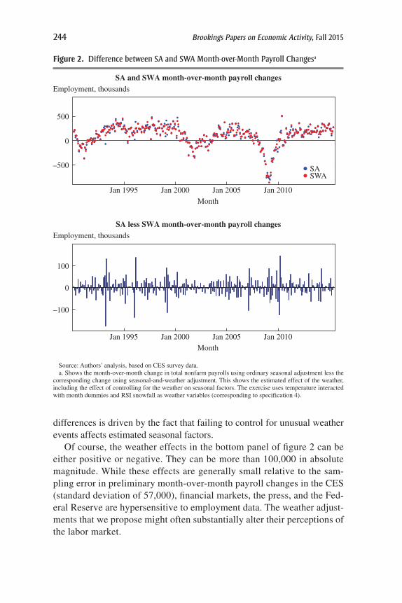
Figure 2 compares total nonfarm payrolls using ordinary seasonal adjust-ment and our seasonal-and-weather adjustment, using this specification. The top panel shows the month-over-month changes in total payrolls with ordinary seasonal adjustment along with the comparable series that we constructed by adjusting for both abnormal weather and normal seasonal patterns. The bottom panel shows the differences in the two series (ordinary SA less SWA). The differences represent the combination of the directly estimated weather effects that are removed from the SWA series and differ-ences between the seasonal factors in the two series. The latter source of

19. Even preventing unusual weather from affecting seasonal factors, the seasonal fac-tors will eventually catch up to climate change because we define unusual weather relative to a rolling 30-year average.


differences is driven by the fact that failing to control for unusual weather events affects estimated seasonal factors.

Of course, the weather effects in the bottom panel of figure 2 can be either positive or negative. They can be more than 100,000 in absolute magnitude. While these effects are generally small relative to the sam-pling error in preliminary month-over-month payroll changes in the CES (standard deviation of 57,000), financial markets, the press, and the Fed-eral Reserve are hypersensitive to employment data. The weather adjust-ments that we propose might often substantially alter their perceptions of the labor market.

Source: Authors’ analysis, based on CES survey data. a. Shows the month-over-month change in total nonfarm payrolls using ordinary seasonal adjustment less the

corresponding change using seasonal-and-weather adjustment. This shows the estimated effect of the weather, including the effect of controlling for the weather on seasonal factors. The exercise uses temperature interacted with month dummies and RSI snowfall as weather variables (corresponding to specification 4).

Employment, thousands

SA and SWA month-over-month payroll changes

SA less SWA month-over-month payroll changesEmployment, thousands

500

Month

SASWA

0

–500

Jan 1995 Jan 2000 Jan 2005 Jan 2010

MonthJan 1995 Jan 2000 Jan 2005 Jan 2010

100

0

–100

Figure 2. Difference between SA and SWA Month-over-Month Payroll Changesa


AUTOCORRELATION Figure 3 shows the autocorrelogram of estimated weather effects. At a lag of one month, the weather effects are significantly negatively autocorrelated. This is because they are estimates of the weather effects in month-over-month changes. Unusually cold weather in month t will lower the change in payrolls during that month, but will boost the change in payrolls for month t + 1, assuming that normal weather returns in month t + 1.

The autocorrelation of the weather effect in payroll changes at lag 12 is also significantly negative. This is because bad weather has some effect on estimated seasonal factors, leading to an “echo” effect of the opposite sign one year later.20 This underscores the importance of integrating the

Source: Authors’ analysis, based on CES survey data.a. Shows the sample autocorrelation function of weather effects, defined as the month-over-month change in total

nonfarm payrolls using ordinary seasonal adjustment less the corresponding change using seasonal-and-weather adjustment. The horizontal dashed lines are the critical values for sample autocorrelations to be statistically significant at the 5 percent level. See note to figure 2.

Autocorrelation

Lag, months5 10 15 20

0

0.2

0.4

–0.2

–0.4

Figure 3. Autocorrelation of Weather Effectsa

20. Wright (2013) argues that the job losses in the winter of 2008–09 produced an echo effect of this sort in subsequent years. The distortionary effects of the Great Recession on seasonals are of course far bigger than the effects of any weather-related disturbances.


weather adjustment into the seasonal adjustment process, as opposed to simply attempting to control for the effect of weather on data that have been seasonally adjusted in the usual way.

RECENT WINTERS In figure 2, the effects of the unusually cold winter of 2013–14 can be seen. We estimate that weather effects lower the month-over-month payroll change for December 2013 by 62,000 and by 64,000 in February 2014. Meanwhile, we estimate that the weather effect raised the payroll change for March 2014 by 85,000 as more normal weather returned. The weather effect was quite consequential, but still does not explain all of the weakness in employment reports during the winter of 2013–14. In March 2015, colder-than-normal weather is estimated to have lowered monthly payroll changes by 36,000.

HISTORICAL EFFECTS The winters of 2013–14 and 2014–15 are far from the biggest weather effects in the sample. The data in February and March 2007 contained a large swing, because that February was colder than usual. That fact was not missed by the Federal Reserve’s Greenbook, which noted in March 2007 that

in February, private nonfarm payroll employment increased only 58,000, as severe winter weather likely contributed to a 62,000 decline in construction employment.21

Payroll changes were weak in April and May 2012. Then–Federal Reserve chairman Ben Bernanke (2012), in testimony to the Joint Eco-nomic Committee, attributed part of this to weather effects, noting that

the unusually warm weather this past winter may have brought forward some hiring in sectors such as construction where activity normally is subdued during the coldest months; thus, some of the slower pace of job gains this spring may have represented a payback for that earlier hiring.

The data in February and March 1999 also contained a big swing, since that February was unseasonably mild. According to our estimates, weather drove the month-over-month change in payrolls up by 90,000 in February 1999 and down by 115,000 the next month. The biggest effect in the sample was March 1993, when weather is estimated to have lowered employment growth by 178,000.22 This is an enormous estimated weather effect, but it does not seem unreasonable: In March 1993, reported nonfarm

21. See page II-1 of the Federal Reserve’s 2007 Greenbook here: http://www.federal reserve.gov/monetarypolicy/files/FOMC20070321gbpt220070314.pdf.

22. Note that there were very big snowstorms in three regions of the country in that month.


payrolls fell by 49,000, while employment growth was robust in the previous and subsequent few months.23

Table 3 lists the 10 months in which the weather effect (the bottom panel of figure 2) is the largest in absolute magnitude. These all occur in the first four months of the year. They turn out to be five pairs of adjacent months as the effects of unusual weather are followed by bounce-backs when more seasonal weather returns.

Table 4 gives the minimum, maximum, and standard deviation of the total weather effect in payroll changes broken out by month.24 The stan-dard deviation is the largest in March (68,000), followed by February (58,000). The standard deviations show that weather effects are poten-tially economically significant in winter and early spring but are rela-tively small in the summer months.

Figure 4 plots the difference between ordinary SA data and SWA data for payroll changes in the construction sector alone (again using specifica-tion 4). Weather effects in the construction sector drive a bit less than half of total weather effects.

23. These are current-data-vintage numbers, with ordinary seasonal adjustment. The first released number for March 1993 was -22,000. The BLS employment situation write-up for that month made reference to the effects of the weather. But the BLS made no attempt to quantify the weather effect.

24. Means are not shown because they are close to zero by construction.

Table 3. Weather Effect in Monthly Payroll Changes, Top 10 Absolute Effectsa

Month Weather effect

March 1993 -178March 2010 +144February 1996 +137January 1996 -137April 1993 +130February 2010 -127March 1999 -115February 2007 -105February 1999 +90March 2007 +87

Source: Authors’ analysis, based on CES survey data.a. Shows the difference in monthly payroll changes (in thousands) that are SA less those that are

SWA, for the 10 months where the effects are biggest in absolute magnitude. These are constructed by applying either the seasonal adjustment or the seasonal-and-weather adjustment to all 150 CES disaggregates, and then adding them up, as described in the text. The exercise uses temperature inter-acted with month dummies and RSI snowfall as weather variables (corresponding to specification 4).

Table 4. Weather Effect in Monthly Payroll Changes, Summary Statisticsa

Month Standard deviation Minimum Maximum

January 42 -137 53February 58 -127 137March 68 -178 144April 44 -57 130May 24 -49 53June 17 -36 27July 22 29 69August 18 -63 17September 15 -24 31October 20 -52 32November 26 -40 76December 38 -66 63Overall 36 -178 144

Source: Authors’ analysis, based on CES survey data.a. Shows the standard deviation, minimum, and maximum of the monthly payroll changes (in

thousands) that are SA less those that are SWA adjusted, broken out by month. See note to table 3.

Source: Authors’ analysis, based on CES survey data.a. See note to figure 2.



0

20

40

–20

–40

Figure 4. Difference between SA and SWA Month-over-Month Payroll Changes in Construction Sectora


In all, the weather adjustment involves estimating 14 parameters in bw for each of the 150 disaggregates for a total of 2,100 parameters. We do not report all of these parameter estimates. Most of the parameters are individ-ually statistically insignificant, but the parameters associated with tempera-ture in December, January, February, and March, as well as the parameters associated with snowfall, are significantly negative for components of con-struction employment.

We deliberately decided against a strategy of setting parameter esti-mates that are individually insignificant to zero. In general, assuming that a parameter is precisely zero because it is not statistically significant seems a dubious approach, and this may be particularly true when doing a bottom-up adjustment for weather effects. For an individual disaggregate, a weather effect might be minor, but these weather effects are likely to be positively correlated across disaggregates, and so the weather effect might be much more important in the aggregate data that we ultimately care about.

PERSISTENCE Purging employment data of the weather effect might make the resulting series more persistent, in much the same way as purging con-sumer price index inflation of the volatile food and energy component makes the resulting core inflation series smoother, as discussed in the introduction. To investigate this, we compare the standard deviation and autocorrelation of month-over-month changes in SA and SWA payroll data, both for total payrolls and for nine industry subaggregates. The results are shown in table 5.

In the aggregate, month-over-month payroll changes show a higher degree of autocorrelation using SWA data than using SA data. This primar-ily reflects the fact that the weather adjustments remove noise from the lev-els data which is a source of negative autocorrelation in month-over-month changes. In fact, in every sector except government, payroll changes show a higher degree of autocorrelation using SWA data than using SA data. The effect is small in most sectors, with the exception of construction, where the proposed weather adjustment raises autocorrelation from 0.59 to 0.77. Particularly in the construction sector, weather adjustment removes noise that is unrelated to the trend, cyclical, or seasonal components. This gives a better measure of the underlying strength of the economy.

II.B. Results with Other Specifications

We also considered the effects on seasonal adjustments from using other specifications discussed in section I. In particular, we considered specifica-tions 5, 6, 7, and 8 as alternatives to specification 4. Specification 5 includes absences from work, specification 6 includes precipitation, specification 7


adds monthly lags to admit richer dynamics, and specification 8 includes weather on the 13th and 14th of the month. Figure 5 shows the difference between SWA data in each of these specifications and the SWA data in specification 4 (that simply used temperature and the RSI index). These charts show that only specification 7 produces noticeably different results. Since the more complicated models make little difference to the weather adjustment, and since simpler models are easier to understand, we prefer specification 4 to specifications 5, 6, and 8.25

Including monthly lags (specification 7) does, however, make a material difference to SWA data, and so we do think of this as an alternative bench-mark approach to weather adjustment. Specification 4 forces the effects of unusual weather on the level of employment to disappear the next month, whereas specification 7 is more flexible regarding the dynamics of weather effects. Figure 6 shows the difference between month-over-month payroll changes using ordinary seasonal adjustment and SWA data using specifica-tion 7. The weather effects for changes in employment are still negatively autocorrelated, but they are much less so when using lags; the first auto-correlation is -0.5 in specification 4, but -0.2 in specification 7.

25. While including absences from work in specification 5 seldom makes a material differ-ence, an exception is September 2008. In this month, the number who reported absence from work due to weather spiked to levels normally observed only in winter. We speculate that this might owe to the fact that Hurricane Ike was moving toward Texas during the survey week.

Table 5. Autocorrelation and Standard Deviation of Month-over-Month Changes in SA and SWA Nonfarm Payroll Data, by Sectora

Sector

Autocorrelation Standard deviation

SA data SWA data SA data SWA data

Mining and logging 0.662 0.686 5.1 5.0Construction 0.586 0.768 39.0 35.9Manufacturing 0.739 0.756 50.4 50.2Trade, transportation, and utilities 0.631 0.651 53.2 52.7Information 0.625 0.645 23.2 23.0Professional and business services 0.572 0.609 53.7 52.9Leisure and hospitality 0.324 0.374 28.6 27.2Other services 0.496 0.533 8.9 8.8Government 0.036 0.034 51.5 51.2Total 0.800 0.840 214.4 210.7

Source: Authors’ analysis, based on CES survey data.a. Reports the first-order autocorrelation and standard deviation of seasonally adjusted (SA) month-

over-month payroll changes (in thousands; total and by industry) and of the corresponding seasonally-and-weather-adjusted (SWA) data. The exercise uses temperature interacted with month dummies and RSI snowfall as weather variables (corresponding to specification 4).


Source: Authors’ analysis, based on CES survey data.a. The four subpanels of this figure show the month-over-month payroll changes using SWA data, where the

weather variables are as in specifications 5, 6, 7, and 8, respectively, less the corresponding SWA data using specification 4. The figure shows the incremental effects of each of these additions to the specification on SWA data.

b. Relative to specification 4, specification 5 adds CPS work absences due to weather. c. Relative to specification 4, specification 6 instead adds precipitation.d. Relative to specification 4, specification 7 instead adds two monthly lags.e. Relative to specification 4, specification 8 adds weather on the 13th and 14th of the current month.


Specification 5b


Specification 6c


Specification 7d


Specification 8e

100

Month

0

–100

100

0

–100

Jan2000

Jan2005

Jan2010

Jan1995

Month

Jan2000

Jan2005

Jan2010

Jan1995

100

Month

0

–100

100

0

–100

Jan2000

Jan2005

Jan2010

Jan1995

Month

Jan2000

Jan2005

Jan2010

Jan1995

Figure 5. Difference between SWA Month-over-Month Payroll Changes in Alternative Specificationsa


Table 6 lists the 10 months in which the weather effects from using this specification are largest in absolute magnitude. Only 5 of these months are also found in table 3. It is interesting to note that table 6 includes only one pair of adjacent months (February and March 2010), while all of the months in table 3 are paired with an adjacent month, which is not entirely surpris-ing because the bounce-back phenomenon from specification 7 is weaker. We computed analogs of tables 4 and 5 for specification 7, but they are similar to the original tables so we do not include them in the paper.

III. NIPA Data

Our focus in this paper has been on the employment report, both because it is the most widely followed economic news release and because it is pos-sible to closely replicate the seasonal adjustment process that the BLS uses

Source: Authors’ analysis, based on CES survey data.a. See note to figure 2. In this figure, lags of weather indicators in the previous two months are also included

(as in specification 7).



0

50

100

150

–100

–50

–150

Figure 6. Difference between SA and SWA Month-over-Month Payroll Changes Using Specification 7a


in the reported CES data. GDP and other NIPA-based economic data are also widely followed and are potentially subject to weather effects. In fact, weather effects could be more important for these series, because harsh weather only affects employment statistics when it causes an employee to miss an entire pay period, but it could have broader effects on NIPA series by lowering hours worked or consumer spending. On the other hand, weather effects on NIPA series could be mitigated by the fact that NIPA data are averaged over a whole quarter, not just a pay period.

III.A. NIPA Weather Adjustment

Unfortunately, the SWA steps described in the previous section cannot be applied to NIPA data because there is no way for researchers to replicate the seasonal adjustment process in these data, let alone to add weather effects to it.26

Table 6. Weather Effect on Monthly Payroll Changes, Top 10 Absolute Effects Using Specification 7a

Month Weather effect

March 1993 -196January 1996 -167February 2010 -165March 2010 +147May 1993 +120May 2003 +118February 2007 -102February 2009 +102April 1990 -98May 1991 -95

Source: Authors’ analysis, based on CES survey data.a. Shows the monthly payroll changes (in thousands) that are SA less those that are SWA, for the

10 months where the effects are biggest in absolute magnitude. These are constructed by applying either the seasonal adjustment or the seasonal-and-weather adjustment to all 150 CES disaggregates, and then adding them up, as described in the text. The exercise uses temperature interacted with month dummies and RSI snowfall along with two monthly lags as weather variables (corresponding to specification 7).

26. Although the BEA compiles NIPA data, seasonal adjustment is done at a highly dis-aggregated level, and many series are passed from other agencies to the BEA in seasonally adjusted form. As noted in Wright (2013) and Manski (2015), while the BEA used to compile not seasonally adjusted NIPA data, they stopped doing so a few years back as a cost-cutting measure. Happily, the June 2015 Survey of Current Business indicated plans to resume pub-lication of not seasonally adjusted aggregate data, but this will still not allow researchers to replicate the seasonal adjustment process.


As an alternative, we instead apply weather adjustments directly to sea-sonally adjusted NIPA aggregates. We consider the model

( )

( ) = µ + µ + µ + µ + f + f + f + f

+ g + g + g + g + g - + e

- - - -

-

y s s s s y y y y

w d w d w d w d w w

t t t t t t t t t

t t t t t t t t t t t

3

,

1 1 2 2 3 3 4 4 1 1 2 2 3 3 4 4

1 1 1 2 1 2 3 1 3 4 1 4 5 2 2 1

where yt is the quarter-over-quarter growth rate of real GDP or some com-ponent thereof, s1t, . . . , s4t are four quarterly dummies,27 w1t is the unusual temperature in quarter t (defined as the simple average of daily values in that quarter), w2t is the unusual snowfall in quarter t (using the RSI index), and d1t, . . . , d4t are four quarterly variables, each of which takes on the value 1 in a particular quarter, -1 in the next quarter, and 0 otherwise. The particular specification in equation 3 has the property that no weather shock can ever have a permanent effect on the level of real GDP—any weather effect on growth has to be “paid back” eventually, although not necessarily in the subsequent quarter, given the lagged dependent variables.28 Our sam-ple period is 1990Q1–2015Q2, using September 2015 vintage data. Coef-ficient estimates are shown in table 7 for real GDP growth and selected

27. The inclusion of these quarterly dummies is motivated by “residual seasonality” discussed further below.

28. Macroeconomic Advisers (2014) find that snowfall effects on growth are followed by effects of opposite sign and roughly equal magnitude in the next quarter.

Table 7. Coefficient Estimates for Equation 3, 1990Q1–2015Q2a

Real GDP

Personal consumption

Private investment

Government expenditures Exports Imports

g1 0.08*** 0.04** 0.19 0.06* 0.26** 0.15*(0.03) (0.02) (0.12) (0.03) (0.11) (0.09)

g2 0.11** 0.06 0.29 -0.08 0.28 0.09(0.05) (0.05) (0.28) (0.06) (0.18) (0.13)

g3 0.04 0.01 -0.33 0.07 0.08 -0.27(0.04) (0.05) (0.37) (0.05) (0.23) (0.19)

g4 0.05 0.02 -0.09 0.07 0.12 -0.10(0.04) (0.04) (0.22) (0.05) (0.14) (0.11)

g5 0.22 -0.04 7.28* -2.83** 0.68 -1.21(0.80) (0.57) (4.17) (1.41) (2.90) (2.85)

Source: Authors’ analysis, based on September 2015 vintage NIPA data.a. Data units are as follows: NIPA growth rates are measured in annualized percentage points, tem-

perature is measured in degrees Celsius, and snowfall is measured in millimeters. Standard errors in parentheses. Statistical significance indicated at the *10 percent, **5 percent, and ***1 percent levels.


components. For real GDP growth, unusual temperature is statistically sig-nificant in the first and second quarters.

We think that the assumption that no weather shock can have a perma-nent effect on the level of GDP is an important and reasonable restriction to impose. Nevertheless, we tested this restriction. We ran a regression of yt on four quarterly dummies, four lags of yt, unusual temperature interacted with quarterly dummies, lags of unusual temperature interacted with quarterly dummies, unusual snowfall, and lagged unusual snowfall. In this specifica-tion, there were 18 free parameters—equation 3 is a special case of this, imposing five constraints that can be tested by a likelihood ratio test. The restriction is not rejected at the 5-percent level for GDP growth or any of the components, except government spending where the p value is 0.04.

Having estimated equation 3, we then compute the dynamic weather effect by comparing the original series to a counterfactual series where all unusual weather indicators are equal to zero (w1t = w2t = 0), but with the same residuals. The difference between the original and counterfactual series is our estimate of the weather effect.

Table 8 shows the quarter-over-quarter growth rates of real GDP and components in 2015Q1 and 2015Q2 both in the data as reported and after our proposed weather adjustment. Weather adjustment raises the estimate of growth in the first quarter from 0.6 percentage point at an annualized

Table 8. Adjustments to NIPA Variable Growth Rates in 2015a

Quarter SA datab SWA datac SSWA datad

Real GDP Q1 0.6 1.5 3.3Q2 3.9 3.1 2.6

Personal consumption Q1 1.7 2.0 2.4Q2 3.6 3.2 3.4

Private investment Q1 8.6 9.6 12.7Q2 5.0 3.1 1.0

Government expenditures Q1 -0.1 0.6 0.9Q2 2.6 2.4 1.3

Exports Q1 -6.0 -3.6 2.2Q2 5.1 3.0 1.0

Imports Q1 7.1 8.4 8.4Q2 3.0 2.2 1.7

Source: Authors’ analysis, based on September 2015 vintage NIPA data.a. Shows the quarter-over-quarter growth rates of real GDP and its five components in 2015Q1 and

2015Q2. All entries are in annualized percentage points.b. Refers to seasonally adjusted data published by the BLS.c. Refers to seasonally-and-weather-adjusted data using the method described in section III.d. Refers to seasonally-and-weather-adjusted data, as described in section III, with a second round of

seasonal adjustment applied using the X-13 default settings.


rate to 1.4 percentage points. However, the estimate of growth in the sec-ond quarter is lowered from 3.7 to 2.8 percentage points. Weather adjust-ment makes the acceleration from the first quarter to the second quarter less marked.

III.B. Residual Seasonality

Our paper is about the effects of weather on economic data, not seasonal adjustment. But an unusual pattern has prevailed for some time in which first-quarter real GDP growth is generally lower than growth later in the year, raising the possibility of “residual seasonality”—the Bureau of Eco-nomic Analysis (BEA)’s reported data may not adequately correct for regu-lar calendar-based patterns. This is a factor, separate from weather, that might have lowered reported growth in 2015Q1. Glenn Rudebusch, Daniel Wilson, and Tim Mahedy (2015) apply the X-12 seasonal filter to reported seasonally adjusted aggregate real GDP and find that their “double adjust-ment” of GDP makes a substantial difference.29

The BEA has subsequently revisited its seasonal adjustment and made changes in the July 2015 annual revision. The changes might have miti-gated residual seasonality, but it is important to note that the BEA has not published a complete historical revision to GDP and its components, instead only reporting improved seasonally adjusted data starting in 2012. We did an exercise in the spirit of Rudebusch, Wilson, and Mahedy (2015) by taking our weather-adjusted aggregate real GDP (and components) data and putting them through the X-13 filter. This double seasonal adjustment is admittedly an ad hoc procedure, especially given that BEA uses a dif-ferent seasonal adjustment method for data after 2012 than for data before 2012; consequently, we treat our procedure’s results with particular cau-tion. Nonetheless, the resulting growth rates in the first two quarters of 2015 are also shown in table 7. After these two adjustments, growth was quite strong in the first quarter, but weaker in the second quarter, which is the opposite of the picture one obtains using published data. It is interesting to note that the “double seasonal adjustment” has an especially large effect on investment and exports, suggesting that these are two areas in which seasonal adjustment procedures might benefit from further investigation.

29. On the other hand, Gilbert and others (2015) find no statistically significant evidence of residual seasonality. The two papers are asking somewhat different questions. Gilbert and others (2015) are asking a testing question, and, while the hypothesis is not rejected, the p values are right on the borderline despite a short sample. Rudebusch, Wilson, and Mahedy (2015) are applying an estimation methodology.


IV. Conclusion

Seasonal effects in macroeconomic data are enormous. These seasonal effects reflect, among other things, the consequences of regular variation in weather over the year. However, the seasonal adjustments that are applied to economic data are not intended to address deviations of weather from seasonal norms. Yet these weather deviations have material effects on macroeconomic data. Recognizing this fact, this paper has operation-alized an approach for simultaneously controlling for both normal sea-sonal patterns and unusual weather effects. Our main focus has been on monthly employment data in the CES, or the “establishment survey.” The effects of unusual weather can be very important, especially in the construction sector and in the winter and early spring months. Monthly payroll changes are somewhat more persistent for seasonally-and-weather adjusted data than for ordinary seasonally adjusted data, sug-gesting that this gives a better measure of the underlying momentum of the economy.

The physical weather indicators considered in this paper are all avail-able on an almost real-time basis—the reporting lag is inconsequential. The National Centers for Environmental Information make daily summaries for 1,600 stations available with a lag of less than 48 hours. In addition, the regional snowfall impact indexes that we use are typically computed and reported within a few days after a snowstorm ends. One weather indicator that we considered is the number of absences from work due to weather. This has a somewhat longer publication lag, but by construction is still available at the time of the employment report.

It would be good if weather adjustments of this sort could be imple-mented by statistical agencies as part of their regular data reporting pro-cess. Because they have access to the underlying source data, they have more flexibility in doing so than the general public—for example, some of the 150 disaggregates in the CES are not available until the first revision. Statistical agencies want data construction to use transparent methods that avoid ad hoc judgmental interventions, and that can be done for weather adjustment. U.S. statistical agencies nevertheless face severe resource con-straints, and weather adjustment might well have an insufficiently high priority. In that case, weather adjustment could be implemented by end users of the data. We do not think weather-adjusted economic data should ever replace the underlying existing data, but as this paper demonstrates, weather adjustment can be a useful supplement to measure underlying eco-nomic momentum.


ACKNOWLEDGMENTS We are grateful to Katharine Abraham, Roc Armenter, Bob Barbera, Mary Bowler, François Gourio, Claudia Sahm, Tom Stark, and the editors for helpful discussions, and to Natsuki Arai for out-standing research assistance. All errors are our sole responsibility. The views expressed here are those of the authors and do not necessarily represent those of the Federal Reserve Bank of Philadelphia or the Federal Reserve System.


References

Andreou, Elena, Eric Ghysels, and Andros Kourtellos. 2010. “Regression Mod-els with Mixed Sampling Frequencies.” Journal of Econometrics 158, no. 2: 246–61.

Bernanke, Ben S. 2012. “Economic Outlook and Policy.” Testimony before the Joint Economic Committee, U.S. Congress, June 7. http://www.federalreserve.gov/newsevents/testimony/bernanke20120607a.htm

Blake, Eric S., Christopher W. Landsea, and Ethan J. Gibney. 2011. “The Deadli-est, Costliest, and Most Intense United States Tropical Cyclones from 1851 to 2010 (and Other Frequently Requested Hurricane Facts).” NOAA Technical Memorandum NWS NHC-6. Miami: National Weather Service, National Hur-ricane Center.

Bloesch, Justin, and François Gourio. 2014. “The Effect of Winter Weather on U.S. Economic Activity.” Economic Perspectives 39, no. 1: 1–20.

Dell, Melissa, Benjamin F. Jones, and Benjamin A. Olken. 2012. “Temperature Shocks and Economic Growth: Evidence from the Last Half Century.” Ameri-can Economic Journal: Macroeconomics 4, no. 3: 66–95.

Faust, Jon, and Jonathan H. Wright. 2013. “Forecasting Inflation.” In Handbook of Economic Forecasting 2A, edited by Graham Elliott and Allan Timmermann. Amsterdam: North-Holland.

Fisher, R. A. 1925. “The Influence of Rainfall on the Yield of Wheat at Rotham-sted.” Philosophical Transactions of the Royal Society of London (Series B) 213: 89–142.

Foote, Christopher L. 2015. “Did Abnormal Weather Affect U.S. Employment Growth in Early 2015?” Current Policy Perspectives no. 15-2. Federal Reserve Bank of Boston.

Ghysels, Eric, Pedro Santa-Clara, and Rossen Valkanov. 2004. “The MIDAS Touch: Mixed Data Sampling Regression Models.” Working Paper. http://docentes. fe.unl.pt/~psc/MIDAS.pdf

———. 2005. “There Is a Risk-Return Trade-Off after All.” Journal of Financial Economics 76, no. 3: 509–48.

Gilbert, Charles E., Norman J. Morin, Andrew D. Paciorek, and Claudia R. Sahm. 2015. “Residual Seasonality in GDP.” FEDS Notes. Washington: Board of Gov-ernors of the Federal Reserve System.

Kocin, Paul J., and Louis W. Uccellini. 2004. “A Snowfall Impact Scale Derived from Northeast Snowfall Distributions.” Bulletin of the American Meteorologi-cal Society 85, no. 2: 177–94.

Ladiray, Dominique, and Benoît Quenneville. 2001. Seasonal Adjustment with the X-11 Method. New York: Springer.

Macroeconomic Advisers. 2014. “Elevated Snowfall Reduced Q1 GDP Growth 1.4 Percentage Points.” Blog post. http://www.macroadvisers.com/2014/04/elevated-snowfall-reduced-q1-gdp-growth-1-4-percentage-points/


Manski, Charles F. 2015. “Communicating Uncertainty in Official Economic Statis-tics: An Appraisal Fifty Years after Morgenstern.” Journal of Economic Literature 53, no. 3: 1–23.

Miguel, Edward, Shanker Satyanath, and Ernest Serengeti. 2004. “Economic Shocks and Civil Conflict: An Instrumental Variables Approach.” Journal of Political Economy 112, no. 4: 725–53.

Rudebusch, Glenn D., Daniel Wilson, and Tim Mahedy. 2015. “The Puzzle of Weak First-Quarter GDP Growth.” Economic Letter no. 2015-16. Federal Reserve Bank of San Francisco.

Squires, Michael F., Jay H. Lawrimore, Richard R. Heim Jr., David A. Robinson, Mathieu R. Gerbush, and Thomas W. Estilow. 2014. “The Regional Snowfall Index.” Bulletin of the American Meteorological Society 95, no. 12: 1835–48.

World Meteorological Organization. 2011. “Guide to Climatological Practices.” WMO-No. 100. Geneva.

Wright, Jonathan H. 2013. “Unseasonal Seasonals?” Brookings Papers on Economic Activity, Fall: 65–110.

Yellen, Janet L. 2014. “The Economic Outlook.” Testimony before the Joint Economic Committee, U.S. Congress, May 7. http://www.federalreserve.gov/newsevents/ testimony/yellen20140507a.htm

———. 2015. “Semiannual Monetary Policy Report to the Congress.” Testimony before the Committee on Financial Services, U.S. House of Representatives, July 15. http://www.federalreserve.gov/newsevents/testimony/yellen20150715a.htm

261

Comments and Discussion

COMMENT BYKATHARINE ABRAHAM I take away two main conclusions from this very useful paper. First, the authors have convinced me that, at least on occasion, unusual weather can cause real problems for interpreting the monthly payroll employment estimates produced by the Bureau of Labor Statistics (BLS). Second, I am also convinced that it is possible to use data on temperature, snowfall, and so on to identify the systematic effects of unusual weather on the payroll employment series and, if desired, to remove those effects from the data. My comments mainly address whether and how the approach the authors have developed might best be applied in the production of official employment statistics. Although the paper focuses primarily on the payroll employment data, as do my comments, similar issues could be raised regarding other economic time series, and I look forward to future work that explores the effects of weather on eco-nomic measurement more broadly.

The payroll employment estimates on which most data users rely are adjusted to remove the effects of normal seasonal variation in the weather along with the effects of other predictable seasonal influences. These adjustments are not intended to account for the effects of weather that is better or worse than usual for the time of year. As the paper demonstrates, the direct effects of unusual weather on employment in the affected month can be relatively large. In addition to its direct effects, unusual weather also can cause distortions in the seasonal factors used to adjust employment estimates in other months. For example, an unusually large snowstorm that depresses employment one February might lead to a lowered expectation for employment levels in the next several Februaries. If the weather were more normal the following February, employment could look stronger than it really was. The approach described in the paper removes both the direct


and the indirect effect of unusual weather from the monthly employment estimates. It would be possible, however, to use these same methods to remove the influence that unusual weather can have on seasonal adjust-ment factors without removing the direct effects of unusual weather on employment in the month in which it occurs. I will come back to this point.

CALENDAR EFFECTS AND WEATHER EFFECTS In reading the paper, I was struck by the parallels between the weather effects that are its subject and the calendar effects that plagued the interpretation of payroll employment data in years past. The calendar effect with the largest effects on the payroll employment series is the so-called 4-week/5-week effect. Depending on the year, there may be either a 4-week interval or a 5-week interval between the weeks in adjacent months that include the 12th of the month and are used to determine the payroll period for which employers are asked to report. The length of this interval can have an important effect on measured employment growth. In construction, to take an example of an industry where the 4-week/5-week effect can be especially important, employment tends to rise through the spring as the weather improves, meaning that the raw growth in employment from March to April is generally larger when the interval between payroll reference periods is longer. Before this was accounted for in estimation, the growth in seasonally adjusted construction employment in a year with 4 weeks between the March and April reference periods that followed years with a 5-week interval tended to look weaker than it actually was, since the seasonal expectation for the March-to-April change was heavily influenced by the larger cumulative upswing associ-ated with a 5-week interval. Conversely, the growth in seasonally adjusted construction employment in a year with 5 weeks between the March and April reference periods could look stronger than it actually was, especially if that year followed years with a 4-week interval (Cano and others 1996).

Through the mid-1990s, discussion of the monthly employment num-bers frequently included statements that were strikingly similar in tone and content to statements about the effects of weather on the numbers quoted by Boldin and Wright. “The Employment Situation: April 1995,” for example, includes the following statement:

The lack of job growth between March and April may have reflected an unusual set of circumstances. . . . The seasonal buildup in services, retail trade, and con-struction from March to April had been relatively large in the previous 3 years (1992–94), partly because in each case there were 5 weeks between the two collections. As a result, this year’s seasonal “expectation” (which is based pri-marily on the prior 3 years) was relatively large. With only 4 weeks separating the surveys, however, the time period for which hiring could take place was

COMMENTS and DISCUSSION 263

reduced. All of this likely made employment in April appear weaker than it actually was. (BLS 1995)

The likelihood that having a 4-week rather than a 5-week interval between March and April had affected the data was noted in news stories at the time (for example, see Georges 1995). Payroll survey estimation procedures that removed the so-called 4-week/5-week effect from the sea-sonally adjusted data were introduced for most industries in 1996 and for construction in 1997.

Different calendar effects have the potential to confound the interpreta-tion of other economic time series. It has long been recognized that flow series such as those for production, shipments, and sales may be affected by the number of working or trading days in the month or by the timing of holidays (Young 1965; Findley and others 1998). In the monthly payroll survey, hours of work tend to be lower than would otherwise be the case when there are fewer workdays during the month or when Good Friday or Labor Day falls during the survey reference period (BLS 2015). Over time, the federal statistical agencies have developed procedures to remove these sorts of calendar effects from published seasonally adjusted estimates.

The present paper proposes that procedures similar to those used to remove calendar effects could be used to remove the effects of unusual weather from published economic data series. Whether this would be a good idea depends on what purpose the adjustments statistical agen-cies make to economic data series should serve. One worthy goal of such adjustments is to produce series that do a better job of capturing underlying trends. A second and somewhat different goal is to produce series that are easier for statistically unsophisticated data users to understand.

With respect to the removal of calendar effects from published season-ally adjusted data, these two goals seem to me to be largely in alignment. That is, analysts are likely to prefer series from which calendar effects have been removed, and I would guess that the typical person on the street also would understand that one does not want, for example, to say employment is growing faster or slower just because the normal seasonal upswing in employment has been measured over a longer or shorter interval.

With respect to the removal of weather effects from published sea-sonally adjusted data, however, the goal of producing a series that better captures an underlying trend may lead to a different conclusion than the goal of producing a series that is easier for statistically unsophisticated data users to understand. Imagine a situation in which a large blizzard had shut down economic activity across much of the country for an extended


period of time. Analysts might find an employment estimate from which the effects of that blizzard have been removed to be more useful as an indi-cator of underlying trends. It is difficult, however, for me to imagine the commissioner of labor statistics reporting such an estimate to the public as the official measure of what had happened to employment during the month. A number that represented what would have happened to employ-ment if there had been no blizzard undoubtedly would be of analytical interest, but it would lack face validity as a representation of reality. For that reason, although I would value changes to its procedures that allowed the BLS to remove the distortions to seasonal factors potentially associ-ated with unusual weather and also to better quantify the direct effects of weather on published employment estimates, I would be uncomfortable with incorporating weather adjustments of the sort described in the paper into the featured payroll employment figures.

HOW THE BLS HANDLES WEATHER ADJUSTMENT As background for thinking about how the BLS might apply the methods developed by Boldin and Wright to improve monthly payroll employment estimates, it may be useful to say a little bit about how unusual weather is handled by current BLS sea-sonal adjustment procedures. Seasonal adjustment of the payroll employ-ment data is implemented by producing seasonally adjusted estimates for detailed estimation cells and then summing the resulting numbers to create seasonally adjusted employment estimates for more aggregated industries and for the nonfarm business sector as a whole. As already mentioned, current BLS procedures are not designed to account directly for the effects of unusual weather, but an estimate for a particular estimation cell that is deemed to be an outlier—as might be the case if unusually good or unusually bad weather had an especially large effect on the number for the estimation cell—may be excluded for the purpose of calculating seasonal factors. Outside the construction industry, however, this rarely happens.

Special procedures to address the effects of unusual weather on con-struction employment have been in place since 1997 (Kropf 1996; Getz 1997). One year earlier, in 1996, new procedures to address the 4-week/ 5-week calendar effect in the payroll employment data had been intro-duced. Because the effects of weather on construction employment are so large, however, usable 4-week/5-week adjustment factors could not be esti-mated for construction without taking weather effects into account, and the implementation of the new 4-week/5-week procedures in construction had to be delayed. This made it a priority to develop some method for address-ing the effects of weather on construction employment.


Within construction, payroll employment estimation, including seasonal adjustment, is carried out at the most detailed industry level for which data are available—either the 5-digit or 6-digit North American Industry Classification System level—and, where possible, separately for each of four regions. Estimates for the relevant detailed industry cells or the detailed industry by region cells then are summed to produce national estimates for published industries. Within construction, the bounds used to determine whether a monthly estimate is an outlier are set to be tighter so that esti-mates are more likely to fall outside the defined bounds and be classified as outliers. Analysts verify apparent outliers in the construction employment estimates as weather-related by checking against information from the National Weather Service and then, if appropriate, they remove the outliers from the data series used to calculate seasonal factors.

As a historical footnote regarding the approach the BLS has adopted to deal with the effects of unusual weather on construction employment, I have been told that when developing its special procedures for construc-tion, the BLS asked the National Weather Service for data on average tem-perature to use in estimating the effects of weather but was turned down. As I understand it, the National Weather Service explained that weather conditions can vary considerably across different parts of the country and information on average temperature would be meaningless. Boldin and Wright make a good case that measures of average weather could in fact have been very useful! That said, recognizing that there is variation in weather conditions across different parts of the country could allow the BLS to improve on Boldin and Wright’s suggested method of accounting for weather effects.

THE CHALLENGE OF GEOGRAPHIC VARIATION Consider the effects of tem-perature on employment. The measure employed in the analysis reported in the paper is a measure of the average across weather stations of the deviation of temperature from its normal level at that weather station in a given month. In many months, however, conditions may be unusually hot in some areas but unusually cold in others. As an illustration, my figure 1, a chart prepared by the High Plains Regional Climate Center and dissemi-nated by the National Weather Service, displays the deviations of the aver-age temperatures from their historical mean levels in different areas for March 2015. Temperatures were considerably below average that month in the Northeast but considerably above average in the Southeast and West. Similar variation may be observed in the monthly data for snow-fall, precipitation, and so on.


This sort of variation would not matter if the effects of deviations from normal weather conditions were both linear and of the same magnitude in all locations. This is unlikely to be the case. The effect of being above or below average with respect to temperature, snow, or other weather con-ditions in a month can vary substantially by region. Weather that was 10 degrees warmer than usual during February, for example, could have a significant effect on employment in Boston but no effect on employment in Phoenix. This implies that a warmer-than-usual February might or might not be associated with higher-than-average employment, depending on where the warmer-than-usual weather occurred. Similarly, an extra six inches of snow might have no effect on employment if it falls in Minne-apolis, but a disastrous impact on employment if it falls in Atlanta. Again, in a month in which average snowfall was greater than expected, it would matter where the extra snow had fallen. The fact that Boldin and Wright obtain better model fits with their preferred snow variable—constructed as

–10 –8 –6 –4 –2 0 2 4 6 8 10

Source: High Plains Regional Climate Center (http://www.hprcc.unl.edu/products/maps/acis/Mar15TDeptUS.png). a. Temperature measured in degrees Fahrenheit.

Figure 1. Departure from Normal Temperature, March 2015a


the weighted average of regional measures of the societal effects of dif-ferent storms rather than average snowfall—is consistent with the idea that deviations of weather from its norm may have different effects in different regions. Thus, important information is lost by relying on national average weather measurements to make the weather adjustments.

As explained in the paper, it would not have been possible for Boldin and Wright to implement a geographically disaggregated weather adjust-ment using published BLS data. The published national employment series refers to the country as a whole, and the state-level employment estimates that the BLS also publishes do not sum to the national estimates. Inter-nally, however, the BLS already makes use of regionally disaggregated estimation cells for construction employment, and conceivably it could do the same for other weather-sensitive industries. This means that, at least in construction, the BLS already has a natural platform in place for incor-porating regional weather information into its estimation procedures. My guess is that weather adjustments based on regional weather data might be at least somewhat larger in size than those reported by Boldin and Wright, though this is of course an empirical question.

THE CHALLENGE OF PAYROLL VARIATION AMONG INDUSTRIES There is one other respect in which the methods outlined by Boldin and Wright might be improved upon. As explained in the paper, the weather variables used for adjusting the employment data are created by weighting weather measure-ments for the 30 days prior to the 12th of the month, with the coefficients of the parametric function used to define the relative weights accorded to different days selected to maximize the fit with national employment data. The important point is that these relative weights are restricted to be the same across all industries. It seems plausible, however, that the rela-tive importance of weather on different days prior to the 12th could vary across industries. It might matter, for example, whether work in the indus-try is done inside or outside, whether employees in the industry are able to work remotely, and whether and how weather affects the demand for the industry’s products or services. I suspect that improving the weights accorded to weather on the different days in the month before the 12th is a second-order issue, but it might nonetheless be worth investigating.

CONCLUSION Supposing that the BLS were to decide to adopt the meth-ods developed by Boldin and Wright—something that I think is very much worth considering—there is still the question of exactly how they would be used. One obvious application would be to use Boldin and Wright’s methods in developing seasonal adjustment factors for the official payroll employment statistics that are not contaminated by the effects of unusual


weather. I also would like the BLS to report the estimated magnitude of the effects of weather on each month’s employment and perhaps even to pre-pare research or supplemental series from which weather effects have been removed. From my perspective, however, to the extent that weather affects the level of employment in a particular month, that should be reflected in the official payroll employment numbers.

REFERENCES FOR THE ABRAHAM COMMENTBLS (Bureau of Labor Statistics). 1995. “The Employment Situation: April 1995.”

News Release. Washington. http://www.bls.gov/news.release/history/empsit_ 050595.txt

———. 2015. “Technical Notes for the Current Employment Statistics Survey.” Washington. http://www.bls.gov/web/empsit/cestn.pdf

Cano, Stephanie, Patricia Getz, Jurgen Kropf, Stuart Scott, and George Stamas. 1996. “Adjusting for a Calendar Effect in Employment Time Series.” In Pro-ceedings of the Survey Research Methods Section. Alexandria: American Sta-tistical Association.

Findley, David F., Brian C. Monsell, William R. Bell, Mark C. Otto, and Bor-Chung Chen. 1998. “New Capabilities and Methods of the X-12-ARIMA Seasonal Adjustment Program.” Journal of Business and Economic Statistics 16, no. 2: 127–52.

Georges, Christopher. 1995. “Economists Say Chances of a Recession Remain Slim, in Spite of Recent Data.” Wall Street Journal, May 8.

Getz, Patricia. 1997. “Improved Seasonal Adjustment for Construction.” Un-published memorandum for George Werking, April 15. Washington: U.S. Bureau of Labor Statistics.

Kropf, Jurgen. 1996. “4/5 Adjustment for Construction, SIC 2015, 2016 and 2017.” Unpublished memorandum for Pat Getz, August 21. Washington: U.S. Bureau of Labor Statistics.

Young, Allan. 1965. “Estimating Trading-Day Variation in Monthly Economic Time Series.” Technical Paper no. 12. Washington: U.S. Bureau of the Census.

COMMENT BYCLAUDIA SAHM1 Michael Boldin and Jonathan Wright introduce a new method for estimating the impact of weather on key economic data series, like monthly payroll employment. Their aim is to provide a

1. I am thankful to Steve Braun, Tyler Cowen, Charles Gilbert, Norman Morin, and Andrew Paciorek for helpful conversations that informed my comments, and to Erik Larsson for his great research assistance. These are my views and are not necessarily shared by others in the Federal Reserve System or the U.S. government.


clearer view of business-cycle fluctuations by removing weather effects. The authors extend a widely used seasonal adjustment algorithm, which already isolates calendar effects and with it the “usual” weather changes over the year. They add a first-stage estimation to the algorithm with a direct measure of weather, so their extended algorithm isolates the impact of both usual and unusual weather.

Trying to estimate the impact of unusual weather events on economic data has a long history among macroeconomic forecasters, so the contri-bution of this paper is a technical improvement: examining a large set of weather measures, using disaggregated industry data, and working within the existing seasonal adjustment framework. While there is more work to be done, this analysis could serve as the basis for systematic weather adjustment in official statistics.

This new seasonal-and-weather adjustment algorithm would be particu-larly useful to individuals who need to interpret economic conditions in real time. The difference between slow demand due to severe weather and slow demand due to an incipient recession is crucial to many economic decisionmakers, including central bank officials setting interest rate policy and business managers weighing new investments. In fact, the importance of isolating weather effects is borne out by the cottage industry of macro-economic forecasters who have provided such estimates for years.

Nonetheless, the winter of 2014 provides a good example of how this paper can add value. During that period, the country experienced one set of weather conditions and one realization of economic activity (though the latter did revise over time), and yet there was a wide range of professional estimates on the output effect from the severe weather. Macroeconomic Advisers (2014) at the time estimated that “elevated snowfall . . . reduced first-quarter GDP growth by 1.4 percentage points,” while an analysis from Goldman Sachs maintained that “weather [would] cause first-quarter GDP to be 0.5 [percentage] point worse than it otherwise would have been” (Goldstein 2014). Federal Reserve staff characterized the weak GDP data this way: “Unusually severe winter weather could account for some, but not all, of the recent unanticipated weakness” (FOMC 2014).

And while few decisions hinge on the exact estimates of weather effects, the extent to which a shift in economic activity can be explained by weather is important. That is because the weather events considered by the authors, such as a severe winter storm, are viewed as a temporary shock and some-thing that most economic decisionmakers should see through. A snow-storm may keep a consumer from buying a car at the end of January, but presumably when the weather clears, she will still buy the car. That kind of


short-term delay—shifting output from one month to the next—should not concern policymakers, though a drop in car purchases due to diminished job prospects would. In real time, when one does not yet know the next month’s or next quarter’s data, the source for a drop in spending can be difficult to determine.

I applaud the authors’ efforts to bring more technical discipline to esti-mating weather effects, yet I have three concerns with the paper. First, I think there needs to be more discussion about the relative importance of unusual weather and the danger of elevating this transitory shock simply because it is something visceral. Business-cycle fluctuations will always be somewhat obscured by noise in the data. Second, I think the authors need to do more to develop the diagnostics of the algorithm. There needs to be clearer guidance on when to use their seasonal-and-weather adjustment similar to the guidance from statistical agencies on when to use the stan-dard seasonal adjustment. And third, in making inferences about weather’s impact, one needs to explore how the weather impact may depend on the business-cycle conditions. I am concerned that this research brings us from removing usual winter weather in usual business-cycle conditions to removing both unusual and usual weather in usual business-cycle condi-tions. This is a step forward, but it may not fully capture how much a par-ticular month’s or quarter’s data are affected by a weather event. Before we begin filtering all our economic data with this new algorithm, we need to think more about the counterfactual—what the world would have looked like without the weather event—and the variation we would be removing from our economic analysis.

High-frequency economic data can be quite noisy. For example, the 90-percent confidence interval on the monthly change in total nonfarm payroll employment is plus or minus 115,000.2 Many of the weather effects that the authors highlight, such as the 64,000 reduction in payroll employment in February 2014, are well within the confidence intervals that reflect sampling and nonsampling error. Still, unusual weather occurs often enough, and comments from Federal Open Market Committee (FOMC) minutes in the month of March for recent years show that we need a reli-able method for isolating such weather effects (see the first column in my table 1). Nonetheless, seasonally-and-weather adjusted data should not give us a false sense of clarity. The second column of my table 1 shows other, non-weather events that were mentioned in the same FOMC minutes

2. See Bureau of Labor Statistics, “Employment Situation Technical Note,” February 5, 2016, http://www.bls.gov/news.release/empsit.tn.htm.


as also obscuring underlying economic conditions. The regularity of some shocks early in the year, such as discretionary changes in fiscal policy, also caution against writing off all the recent first-quarter weakness in recent years as an inability to remove calendar or weather effects.

The authors weather-adjust all the data series regardless of how well the weather model fits an industry series, but this decision is at odds with the standard use of seasonal adjustment in official statistics. For example, consider this statement from the U.S. Census Bureau:

The Census Bureau performs seasonal adjustment of a time series of estimates only given clear evidence of seasonal behavior and only when the adjustment passes a suitable set of diagnostic tests. (McDonald-Johnson and others 2010)

Charles Gilbert and others (2015) provide an example of using such diagnostic tests to examine residual seasonality in output data. Stability of the adjustment factors is a guiding principle for the decision as to when it is appropriate to seasonally adjust a data series. One might view the diag-nostic tests for seasonal adjustment in official series as too stringent, but there needs to be further analysis of how stable the seasonal-and-weather adjustments in the Boldin and Wright paper are. The stability of the weather impact estimates may be improved by focusing on series that show a clear weather impact, such as construction employment.

Finally, it is important to take a step back and think about the varia-tion being removed with the seasonal-and-weather adjustment. Consum-ers, employers, and even policymakers experience the economy with all its seasonal and weather-related variation, so using adjusted data misses the opportunity to study that variation. Robert Barsky and Jeffrey Miron (1989) argue, for example, that seasonal variation could be used to test macroeconomic models, yet macroeconomic studies with not seasonally adjusted data are exceedingly rare. Of related concern, the weather impact

Table 1. Events Noted as Obscuring Underlying Economic Conditions in March FOMC Minutes, 2010–15

Weather Non-weather

2015 “unseasonably cold winter weather” “labor disputes at West Coast ports”2014 “unusually cold and snowy winter weather” “partial government shutdown”2013 — “federal spending sequestration”2012 “unseasonably warm weather” —2011 “weather-related distortions in various

indicators”“earthquake, tsunami”

2010 “adverse effects of the snowstorms” “waning effects of fiscal stimulus”

Sources: FOMC (2010, 2011, 2012, 2013, 2014, 2015).


may not be neatly separable from underlying economic conditions. Alan Auerbach and Yuriy Gorodnichenko (2012) argue that the impact of dis-cretionary government spending on output (the fiscal multiplier) is larger in recessions than in expansions. Likewise—and a point acknowledged but not explored by the authors—a severe snowstorm may have a different impact on activity during a recession than during an expansion. This would complicate the full removal of weather effects, and the removal, even par-tially, may sacrifice some information on underlying economic conditions.

As a simple example of how weather might interact with the busi-ness cycle conditions, I estimated a standard model of monthly retail sales growth (RS Growth), which includes heating degree days (HDD), con-sumer sentiment (Sent), and an interaction between them. I chose sentiment as a business cycle indicator because, unlike some employment series, it does not vary with the weather measure in the regression. The results of the estimation are represented below, with standard errors in parentheses.3

RS Growth HDDt t=( )

−( )

+0 280 045

0 250 047

0 140

..

..

...

. .. .

047

0 10 0 090 042 0 049

1( )+ −

( ) ( )

−HDD

Sent H

t

t DDD Sentt t×

Unusually cold weather, which is a positive heating degree day reading, depresses the growth in retail spending in the current month and boosts it in the subsequent month, highlighting the transitory nature of weather shocks. This is a well-known feature of retail sales growth—an example of how weather estimates are often done. The positive association between retail sales growth and sentiment is also standard. The additional feature of this simple model, as shown in my figure 1, is that unusually cold weather weighs more on retail spending growth at times when sentiment is high, measured as one standard deviation above average.

Intuitively, it makes sense that if economic activity is picking up and consumer sentiment is high, a severe winter storm would imply a large drag on growth, since there is more growth to disrupt relative to the counter-

3. The regression is estimated with monthly data from January 1999 to July 2015, and the R2 is 0.17. All of the coefficients are statistically significant at the 10 percent level. The dependent variable is seasonally adjusted retail sales excluding autos, gasoline, and build-ing materials; this is the portion of the retail sales data used by the Bureau of Economic Analysis in its estimate of personal consumption expenditures, and it accounts for roughly one-fifth of GDP.


factual world of normal weather. In isolating the impact of weather, it is better to remove the “average sentiment” and heating degree effect, which is closest in spirit to the authors’ seasonal and weather-adjusted data but that does not mean that all of the weather impact has been removed. And this also leaves open an interesting question about how consumers or employers interpret these weather shocks, which in real time would be hard to distinguish from other economic shocks. With its careful technical treat-ment of estimating weather effects, this paper should serve as an invitation to think more about what weather’s impact is on the economy.

REFERENCES FOR THE SAHM COMMENT

Auerbach, Alan J., and Yuriy Gorodnichenko. 2012. “Measuring the Output Responses to Fiscal Policy.” American Economic Journal: Economic Policy 4, no. 2: 1–27.

Barsky, Robert B., and Jeffrey A. Miron. 1989. “The Seasonal Cycle and the Busi-ness Cycle.” Journal of Political Economy 97, no. 3: 503–34.

FOMC (Federal Open Market Committee). 2010. “Minutes of the Federal Open Market Committee: March 16, 2010.” Washington: Board of Governors of the Federal Reserve System. http://www.federalreserve.gov/monetarypolicy/ fomcminutes20100316.htm

Percent

Average monthly growth

–0.2

0

0.2

Low sentiment Average sentiment High sentiment

Figure 1. Impact of Severe Cold on Retail Sales Growth by Business Cycle Conditions


———. 2011. “Minutes of the Federal Open Market Committee: March 15, 2011.” Washington: Board of Governors of the Federal Reserve System. http://www.federalreserve.gov/monetarypolicy/fomcminutes20110315.htm

———. 2012. “Minutes of the Federal Open Market Committee: March 13, 2012.” Washington: Board of Governors of the Federal Reserve System. http://www.federalreserve.gov/monetarypolicy/fomcminutes20120313.htm

———. 2013. “Minutes of the Federal Open Market Committee: March 19–20, 2013.” Washington: Board of Governors of the Federal Reserve System. http://www.federalreserve.gov/monetarypolicy/fomcminutes20130320.htm



Gilbert, Charles E., Norman J. Morin, Andrew D. Paciorek, and Claudia R. Sahm. 2015. “Residual Seasonality in GDP.” FEDS Notes. Washington: Board of Governors of the Federal Reserve System.

Goldstein, Steve. 2014. “March Was Colder but Less Snowy Than Usual, So Data Should Get Lift, Forecaster Says.” Blog post, April 1. MarketWatch.

Macroeconomic Advisers. 2014. “Elevated Snowfall Reduced Q1 GDP Growth 1.4 Percentage Points.” Blog post, April 16. http://www.macroadvisers.com/ 2014/04/elevated-snowfall-reduced-q1-gdp-growth-1-4-percentage-points/

McDonald-Johnson, Kathleen M., Brian Monsell, Ryan Fescina, Roxanne Feldpausch, Catherine C. Harvill Hood, and Monica Wroblewski. 2010. “Seasonal Adjustment Diagnostics.” Census Bureau Guideline, Version 1.1. Washington: U.S. Census Bureau. https://www.census.gov/ts/papers/G18-0_v1.1_Seasonal_Adjustment.pdf

GENERAL DISCUSSION Jonathan Pingle wondered if Michael Boldin and Jonathan Wright had checked the stability of the coefficients that they estimated in their model. Pingle noted that, in his own work, the impact of snowfall appeared to have changed over the course of the past three decades.

Pingle also wondered if there is evidence of asymmetry in the data; that is, does the weather being better-than-normal by a certain amount have an equal and opposite effect as the weather being worse than normal by the same amount? As an example, he noted that it is often the case where it seems like a very cold March will be followed by instant bounce-back in April, but a very warm March sometimes seems to pull forward seasonal inflows for several months. He was curious if that kind of asymmetry might be driving some of the lagged effects mentioned in the paper.


Along similar lines, David Romer wondered about the assumption often made by short-term forecasters of full bounce-back due to the effects of weather; on average, that is, are the negative effects of bad weather made up the following month as the weather on average returns to normal? For example, if weather reduced employment in one month by 50,000 jobs, should it really be assumed that the next month is going to add those 50,000 jobs? Perhaps that would make sense, he noted, in a world where firms have a set number of people they want to hire, and they can just go out and get them. But perhaps matches that do not occur in one month are not magically formed in the next.

Pingle wondered if Boldin and Wright had given any thought to the implications of the difference observed between the weather effects in the initial release of the Current Employment Statistics (CES) data and the weather effects in the revised data. Sometimes, the initial release seems to lack a significant weather effect, but it is more pronounced upon revision. He wondered if it could be the case that more weather-affected establish-ments were not reporting in as timely a manner. If that were the case, then applying Boldin and Wright’s methodology to the initial release of the data could offset a negative weather effect not yet in the data, thus overstating the month’s employment.

Jeff Campbell wondered about the implications of the model as it relates to forecasting. He agreed with discussant Katharine Abraham, who had noted that one of the key goals of weather adjustment might be to pro-duce data series more suitable for short-term forecasting, noting that there are alternative means of doing that. In the methodology implemented by Boldin and Wright, weather adjustment is applied to an economic series before being put into a forecasting model. Campbell wondered if a prin-cipal component of the weather adjustment could be applied to the fore-casting model itself. Alan Blinder took issue with the claim that a goal of adjusting data in the first place is to make them more suitable for short-term forecasters, noting that a broader group of professionals is interested in adjusted data. Campbell also wondered if authors had any results relating to inventories.

Abraham also had suggested that another goal of adjusting data might be to produce series that are easier for ordinary people to understand. Blinder took strong issue with this suggestion as well. He noted that adjusted data are used by only a small cadre of experts, and that ordinary people live in a real world that is not seasonally or weather adjusted. For example, if an ordinary person wanted to get a job in retail, it would be easier for her to look during the Christmas season rather than in January; if she wanted to


be a lifeguard, she would have an easier time finding a job in early sum-mer rather than in October. For the small cadre of experts, however, these adjustments are really useful.

Valerie Ramey, who had dealt extensively with weather effects in her work, remarked on how useful the Boldin and Wright methodology was. She appreciated Boldin and Wright’s systematic approach to removing large weather-related outliers from the data. Ramey suggested that some of the assumptions made by Boldin and Wright were appropriate, while others might need to be loosened. She agreed that the effects of lags considered by Boldin and Wright were definitely necessary, citing her experience with auto assembly plants. She recounted the great blizzard of 1978, in which assembly line workers were able to return to work, but the plants remained closed because the blizzard had prevented the delivery of parts.

Ramey took issue with the authors’ model identification in two aspects. First, she questioned the assumption that weather occurring after the 12th day of the month should not have any effect on employment data. In most surveys that measure employment data, the reference period is generally the calendar week or pay period that contains the 12th day of the month. She suggested that the authors consider at least a few days after the 12th, noting that forecasts of abnormal weather in the near future may actually affect employment in the present. Steve Braun echoed Ramey’s concerns, noting that if the 12th occurred on a Sunday, then as many as five extra days might need to be considered.

Ramey also questioned the assumption that unusual weather events do not have permanent effects, citing a growing environmental literature. She noted, as examples, that hurricanes hitting small islands, or Hurricane Katrina hitting New Orleans, certainly had some permanent effects on employment.

Robert Gordon commented on the relationship between GDP and payroll employment, namely productivity. Payroll data do not reflect big weather events as strongly as data for GDP, resulting in overinflated estimates of productivity and extremely high positive correlations between output and productivity. Looking at detrended levels of output productivity over the last five to twenty years, Gordon noted it is clear that there is no longer any short-term positive correlation between productivity and output. He posited that the historically low productivity growth data over the last five years reflect structural rather than cyclical changes in the economy.

Braun praised Boldin and Wright’s methods as clear improvements over previous efforts to model weather adjustment. He suggested that it might be useful to apply the model not only to employment, as Boldin and Wright


do, but also to measures such as work week and man-hours, which are more sensitive to the effects of weather. He noted that the exercise might be particularly interesting because the correlation between man-hours and GDP is much stronger than between employment and GDP, a concern raised earlier by Gordon.

Christopher Carroll pointed out that there may be substantively impor-tant issues on which forecasters could reach the wrong conclusions about the underlying momentum of the economy if they did not take into account some kind of weather adjustment in their forecasts. According to Boldin and Wright, the serial correlation of growth is substantially greater when adjusted for weather. Historically, the debate about whether or not the serial correlation of a variable was important centered on whether or not con-sumption followed a random walk. Carroll believed that evidence seemed overwhelming that there was a lot more momentum in consumption growth than was apparent originally because weather effects were adding noise to quarterly numbers. He was enthusiastic about the work put forward by Boldin and Wright, speculating that it might have real consequences for how business cycle models are calibrated.

Andrew Abel commented on the differences between the Current Popu-lation Survey (CPS) and the CES in how they measure employment. In the CES, abnormal weather that prevents people from going to work reduces the payroll employment count, since the data are based on surveys of busi-nesses. In the CPS, however, an individual who does not go to work due to abnormal weather may still be counted as employed if weather or some other reason is given for not working. Abel wondered if Boldin and Wright were aware of how many people responded to the CPS in this way, and whether the magnitudes compared with the magnitudes that the authors calculated with their weather-adjustment model.

Adele Morris was interested in understanding regional and local labor market vulnerabilities to extreme weather events, and promoted Abraham’s suggestion to have regional data adjustments in addition to the national adjustments made by Boldin and Wright. If more extreme weather events were on the horizon, it would be beneficial to have a deeper understanding of the regional and local vulnerabilities. In addition to trying to take out weather information to see what remains, she suggested that what is taken out may be extremely interesting to people who are thinking about local or regional policies to adapt to a changing climate.

Discussant Claudia Sahm brought up the question of when it is appropri-ate to adjust for weather, and which series to adjust. One could argue that the Census is too conservative in deciding which series to adjust, that is,


it should be adjusting more series than it currently does. When adjusting a series for weather affects, it is important that the effect pulled out is in fact a weather effect, and not some other kind of effect. It is clear that employment data in construction should be adjusted because there are clear and stable patterns. However, other series might not benefit from weather adjustment, since it might not be clear that they are stable or significant enough.

Sahm believed that looking at disaggregated data could be important, for instance in analyzing the behaviors of consumer spending. In the case of motor vehicle consumption, bad weather may deter the purchase of a vehicle in one month, but the vehicle would almost certainly be purchased in the next month. On the other hand, if a consumer was prevented from going out to dinner or purchasing something for the holidays, persistent bad weather may actually prevent those transactions from ever happening in the near future.

Responding to Pingle’s and Romer’s question of asymmetry, Wright noted that he and Boldin looked into the issue, but did not find much evidence. The authors described an experiment in which they considered weather in the previous month and weather in the previous 2 months; they found that bad weather one month prior did lower the level of employment, but 2 months prior did not. He conceded that it is not correct to say that there is complete bounce-back immediately, but that it is not very far off.

In response to Ramey’s and Braun’s concerns about abnormal weather after the 12th day of the month, Wright stated that he and Boldin did test the effects of weather after the 12th day of the month, but only in a very crude way; by adding extra variables for the weather on the 13th and 14th, Boldin and Wright found that they were insignificant in the aggre-gate. Wright agreed with Ramey that some weather events may have a per-manent impact, but argued that her framework might not be the right way to think about what the model was meant to isolate, such as a snowy winter or colder-than-normal January.

Wright responded to the question raised by Sahm regarding which series to adjust. If the ultimate interest is in aggregates rather than disaggregates, then Wright believes that statistical agencies are currently too conservative and too willing to just decide not to seasonally adjust a series at all.

Wright noted that while technology for weather adjustment is avail-able and hopefully useful, it is not intended to replace the data. It is useful to have some way to figure out what the effects of weather are, and for statistical agencies to have some advantage in being able to do that.

weather-adjusting economic data - brookings institution · weather-adjusting economic data ......

Documents