weather and atmospheric effects on the measurement …
TRANSCRIPT

Optical Systems Group
RCC 469-17
WEATHER AND ATMOSPHERIC EFFECTS ON THE MEASUREMENT
AND USE OF ELECTRO-OPTICAL SIGNATURE DATA
DISTRIBUTION STATEMENT A. Approved for public release. Review completed by the AMRDEC Public Affairs Office January 31 2017 and
PR2594.
ABERDEEN TEST CENTER DUGWAY PROVING GROUND
REAGAN TEST SITE REDSTONE TEST CENTER
WHITE SANDS MISSILE RANGE YUMA PROVING GROUND
NAVAL AIR WARFARE CENTER AIRCRAFT DIVISION NAVAL AIR WARFARE CENTER WEAPONS DIVISION
NAVAL UNDERSEA WARFARE CENTER DIVISION, KEYPORT NAVAL UNDERSEA WARFARE CENTER DIVISION, NEWPORT
PACIFIC MISSILE RANGE FACILITY
30TH SPACE WING 45TH SPACE WING 96TH TEST WING
412TH TEST WING ARNOLD ENGINEERING DEVELOPMENT COMPLEX
NATIONAL AERONAUTICS AND SPACE ADMINISTRATION

This page intentionally left blank.

DOCUMENT 469-17
WEATHER AND ATMOSPHERIC EFFECTS ON THE MEASUREMENT AND USE OF ELECTRO-OPTICAL SIGNATURE DATA
February 2017
Prepared by
OPTICAL SYSTEMS GROUP
Published by
Secretariat Range Commanders Council
U.S. Army White Sands Missile Range New Mexico 88002-5110

This page intentionally left blank.
Weather and Atmospheric Effects on the Measurement and Use of Electro-Optical Signature Data RCC 469-17 February 2017
iii
Table of Contents Preface .............................................................................................................................................v
Acronyms ..................................................................................................................................... vii
Introduction ....................................................................................................................... 1
Background ....................................................................................................................... 1
Outline ................................................................................................................................ 5
Radiometric and Photometric Quantities, Symbols, Units, and Definitions ............... 5
4.1 Some Notes about Notation ................................................................................................ 6 4.2 Radiometric Quantities, Symbols, Units, and Definitions .................................................. 7 4.3 Photometric Quantities, Symbols, Units, and Definitions ................................................ 16
Atmospheric Correction of Measured Target Signature Data and Applying Atmospheric Effects when using Target Signature Data ............................................ 23
5.1 Atmospheric Correction of Target Data Collected with a Radiometer or Imaging Radiometer ........................................................................................................................ 24
5.2 Atmospheric Correction of Target Data Collected with a Photometer or Imaging Photometer ........................................................................................................................ 36
Weather/Atmospheric Effects on Electro-Optical Systems ........................................ 39
Atmospheric Transmission Models ............................................................................... 54
Conclusions ...................................................................................................................... 56
Appendix A. Example Calculations ................................................................................... A-1
Appendix B. Citations ......................................................................................................... B-1
Table of Figures Figure 1. Electromagnetic Spectrum and a Portion of the Optical Region Limited to
25 µm .......................................................................................................................2 Figure 2. Relative Spectral Response of the Eye ..................................................................16 Figure 3. Atmospheric Correction Process............................................................................24 Figure 4. H20 Transmission ...................................................................................................31 Figure 5. CO2 Transmission ..................................................................................................32 Figure 6. Spectral Transmission of Measurement Paths .......................................................33 Figure 7. Relative Apparent Radiance vs. Range (100 °C BB) ............................................33 Figure 8. Relative Spectral Distribution (100 °C BB) ..........................................................34 Figure 9. Lower Layers of the Earth’s Atmosphere ..............................................................39 Figure 10. Molecular Absorption at Electro-Optical Wavelengths .........................................41

Weather and Atmospheric Effects on the Measurement and Use of Electro-Optical Signature Data RCC 469-17 February 2017
iv
Figure 11. Transmission near Atmospheric Windows (0.2 – 0.4 μm) ....................................42 Figure 12. Transmission near Atmospheric Windows (0.4 – 0.7 μm) ....................................43 Figure 13. Transmission near Atmospheric Windows (1 – 1.5 μm) .......................................43 Figure 14. Transmission near Atmospheric Windows (2 – 3 μm) ..........................................44 Figure 15. Transmission near Atmospheric Windows (3 – 5 μm) ..........................................44 Figure 16. Transmission near Atmospheric Windows (8 – 12 μm) ........................................45 Figure 17. Transmission in the Mid-Wave Infrared Band ......................................................46 Figure 18. Estimated CO2 Mixing Ratio Over Time ...............................................................47 Figure 19. Effective Water Vapor vs. Altitude .......................................................................48 Figure 20. Ultraviolet Transmission, Mid-Latitude ................................................................49 Figure 21. Ultraviolet Transmission, Desert ...........................................................................50 Figure 22. Ultraviolet Transmission, Tropical ........................................................................50 Figure 23. Ultraviolet Transmission, Sub-Arctic ....................................................................51 Figure 24. Scattering Efficiency Factor vs. Wavelength/Scatterer Size .................................52
Table of Tables Table 1. General Sub-Region Terms of the Optical Spectrum ..............................................2 Table 2. Some Laser Wavelengths of Interest .......................................................................3 Table 3. Basic Radiometric Quantities, Symbols, and Units .................................................6 Table 4. Relative Spectral Response of the Eye ....................................................................7 Table 5. Basic Photometric Quantities, Symbols, and Units ...............................................17 Table 6. Constituents of Earth’s Atmosphere ......................................................................40 Table 7. Absorption by Atmospheric Molecules .................................................................41 Table 8. Approximate Size of Atmospheric Aerosols .........................................................53 Table 9. Some Atmospheric Transmission Software ...........................................................54

Weather and Atmospheric Effects on the Measurement and Use of Electro-Optical Signature Data RCC 469-17 February 2017
v
Preface Weather has an adverse effect on the operation of electro-optical systems. Permanent and
variable constituents along atmospheric paths in the earth’s troposphere attenuate electro-optical energy. Radiation from these atmospheric constituents also contaminates the radiation from targets. Some weather conditions, such as clouds and fogs, negate the propagation of all electro-optical wavelengths. Some clear-air atmospheric constituents negate the propagation of certain electro-optical wavelengths. Within certain spectral bands, atmospheric attenuation is not severe, allowing the use of these bands for military operations.
Measured target signature data is less than actual target signatures due to atmospheric attenuation. Therefore, to obtain actual target signature data, measured data must be corrected for the effects of atmospheric path attenuation and path radiance.
This RCC report quantifies weather/atmospheric effects and the problem of correcting and applying measured data. It provides glossaries of electro-optical and weather terms related to EO/IR test environments (parameters, quantity names, symbols, units, equations, terms, and definitions). It concentrates on weather/atmospheric test environments that affect the determination and use of target electro-optical signatures.
Detailed methodologies for correcting measured data to obtain actual target signature data for various weather/atmospheric conditions are presented. Also, a method for applying operational conditions to the target signature data to obtain estimates of military system’s capability and limitations is presented.
For questions regarding this document, please contact the Range Commanders Council Secretariat office.
Secretariat, Range Commanders Council ATTN: CSTE-WS-RCC 1510 Headquarters Avenue White Sands Missile Range, New Mexico 88002-5110 Telephone: (575) 678-1107, DSN 258-1107 E-mail: [email protected]

Weather and Atmospheric Effects on the Measurement and Use of Electro-Optical Signature Data RCC 469-17 February 2017
vi
This page intentionally left blank.

Weather and Atmospheric Effects on the Measurement and Use of Electro-Optical Signature Data RCC 469-17 February 2017
vii
Acronyms μm micrometer AFRL Air Force Research Laboratory CIE International Commission on Illumination CO2 carbon dioxide EO electro-optical EOSAEL Electro-Optical Systems Atmospheric Effects Library FIR far infrared FOV field of view FUV far ultraviolet H2O water HEL high-energy laser IFOV instantaneous field of view IR infrared LWIR long-wave infrared MG Meteorology Group mm millimeter MWIR mid-wave infrared NIR near infrared nm nanometer O2 oxygen O3 ozone SI International System of Units SNR signal-to-noise ratio sr steradian SWIR short-wave infrared UV ultraviolet VIS visible

Weather and Atmospheric Effects on the Measurement and Use of Electro-Optical Signature Data RCC 469-17 February 2017
viii
This page intentionally left blank.

Weather and Atmospheric Effects on the Measurement and Use of Electro-Optical Signature Data RCC 469-17 February 2017
1
Introduction Weather and atmospheric constituents limit the capability of all remote sensing electro-
optical (EO) systems. Weather and atmospheric backgrounds/foregrounds result in system noise. The path between a system and a target attenuates the energy from a target. Even when the atmosphere appears visually clear, atmospheric effects degrade target signature data.
Target EO signature measurements are made through an attenuating atmospheric path and in the presence of varying atmospheric backgrounds and foregrounds. Weapon systems and weapon system models engage targets through operational atmospheric paths and with backgrounds that are different from what existed when signature measurements were made. The apparent signatures of targets observed through atmospheric paths are different from actual target signatures in both cases. Remote measurements produce apparent signature data. Users of signature data require actual target signature data. Measured apparent signature data must be corrected to obtain actual target signatures. Some methods used to correct measured data may produce target signature data having significant errors. This document will provide a methodology for accounting for atmospheric effects and converting measured signature data to actual target signature data.
Users of measured/corrected target signature data must apply parameters that describe their particular weapon system and operational atmospheric/weather conditions to the measured/corrected target signature data in order to estimate their system’s performance capabilities and limitations in various scenarios.
This document does not deal with the significant problems associated with measurement system characterization and calibration and the accurate measurement of apparent target signatures. The RCC document 809-101 describes that process. This document deals with weather/atmospheric effects and the problem of correcting and applying measured data. It provides glossaries of EO and weather terms related to EO/infrared (IR) test environments (parameters, quantity names, symbols, units, equations, terms, and definitions). It concentrates on weather/atmospheric test environments that affect the determination and use of target EO signatures.
The primary purpose of this document is to quantify weather and atmospheric effects as applied to EO systems. It defines applicable weather and atmospheric quantities and their determination, defines applicable radiometric and photometric quantities, and describes the processes required to account for atmospheric/weather effects in the correction of measured data and in the use of that data.
Background Radiation from EO sources constitutes a very small portion of the electromagnetic
spectrum. It includes ultraviolet (UV), visible, and IR radiation. This type of radiation is
1 Range Commanders Council. Standards and Procedures for Application of Radiometric Sensors. 809-10. July 2010. May be superseded by update. Retrieved 28 July 2016. Available at http://www.wsmr.army.mil/RCCsite/Documents/809-10_Standards_and_Procedures_for_Application_of_Radiometric_Sensors/.

Weather and Atmospheric Effects on the Measurement and Use of Electro-Optical Signature Data RCC 469-17 February 2017
2
generally characterized by its wavelength (λ) or wavenumber (cm−1). The EO region of the electromagnetic spectrum is shown in Figure 1.
Figure 1. Electromagnetic Spectrum and a Portion of the Optical
Region Limited to 25 µm
The authoritative International Commission on Illumination (CIE) considers the electromagnetic region between x-rays (<0.1 micrometers [μm]) and millimeterwave (1 millimeter [mm] = 1000 μm) as optical radiation. The CIE has recommended the band designations shown in Table 1. The common military band designations (spectral bands of reasonable atmospheric transmission) are also shown in the table.
Table 1. General Sub-Region Terms of the Optical Spectrum CIE
Recommended Astrophysics Atmospheric Science Nominal Military Band
(Micrometers) Far UV (FUV) 0.01 to 0.1 Extreme UV 0.01 to 0.121

Weather and Atmospheric Effects on the Measurement and Use of Electro-Optical Signature Data RCC 469-17 February 2017
3
Table 1. General Sub-Region Terms of the Optical Spectrum CIE
Recommended Astrophysics Atmospheric Science Nominal Military Band
(Micrometers) Lyman-alpha 0.121-0.122 FUV 0.122 to 0.2 Mid-UV 0.2 to 0.3 Near UV 0.3 to 0.4 Vacuum UV 0.01 to 0.2 UV-C UV-C UV-C 0.1 to 0.28 UV-B UV-B UV-B 0.28 to 0.315 Solar Blind UV 0.2 to 0.315 UV-A* UV-A* 0.315 to 0.38 UV-A 0.32 to 0.4 Visible (VIS) VIS 0.36 to 0.83 (‡) VIS 0.38 to 0.78 VIS 0.4 to 0.7 Near-IR (NIR) 0.7 to 4 IR 0.7 to 1000 NIR 0.76 to 1.4 IR-A 0.78 to 1.4 NIR 0.75 to 1.83 IR-B Middle IR 1.4 to 3 Short-Wave IR (SWIR) 1.83 to 2.7 Mid-Wave IR (MWIR) 2.7 to 6 IR-C Far IR (FIR) 3 to 1000 Thermal IR 4 to 50 Long-Wave IR (LWIR) 6 to 30 FIR, also Terahertz IR 30-1000 FIR 50 to 1000 * Global solar UV index designates UV type A (UV-A) as 0.315 μm to 0.4 μm. ‡ The spectral limits of the spectral luminous efficiency for photopic vision (Reference 3c).
In addition to passive EO systems, which typically (in the lower atmosphere) must operate in one of the designated bands of relatively good atmospheric transmission, there are laser wavelengths of interest; particularly those wavelengths associated with high-energy laser (HEL) systems, laser designators, and lidars. Some of the HELs and their associated weapon systems are shown in Table 2.
Table 2. Some Laser Wavelengths of Interest Laser
Wavelength (μ) Function Weapon System
0.532 Frequency Doubled Yttrium Aluminum Garnet
Vision/System Impairment
1.03 Target illumination Airborne Laser (ABL)

Weather and Atmospheric Effects on the Measurement and Use of Electro-Optical Signature Data RCC 469-17 February 2017
4
Table 2. Some Laser Wavelengths of Interest Laser
Wavelength (μ) Function Weapon System
1.064 Beacon Illumination ABL 1.315 HEL ABL and Advanced Tactical Laser 1.319 Surrogate HEL ABL 2.6-3.0 Hydrogen Fluoride (HEL) Space-Based Laser 3.8 Deuterium Fluoride (HEL) Tactical High Energy Laser; Mobile
Tactical High Energy Laser; Mid-Infrared Advanced Chemical Laser
5-6 Carbon Monoxide Laser (HEL) Possible Threat Laser 10.6 Carbon Dioxide Ranging Laser ABL
It is well-known that EO weapons are not all-weather systems. Under certain conditions (e.g., clouds, fog, smoke, or dust between a system and a target) EO systems operating at any wavelength have a severely limited capability.
Even when atmospheric conditions might be considered clear, the atmosphere attenuates EO radiation from a target. At certain wavelengths transmission is always near zero, even for short, clear atmospheric paths. At other wavelengths transmission may often be near 100% (bands of relatively good clear-air transmission are called atmospheric windows).
When a target signature is measured, the atmospheric attenuation along the measurement path results in a measured apparent signature that is less than what would exist if there was no attenuation (the actual target signature). Since actual target signatures are required by users of measured signature data, the measured data must be corrected for atmospheric attenuation, path radiance, and background radiation. This process requires an accurate determination of the atmospheric path spectral transmission and path spectral radiance in the measurement spectral band.
Computer models are available to provide an estimate of the spectral transmission coefficients (and path spectral radiance) for a wide range of atmospheric paths. The Air Force Research Laboratory (AFRL) MODTRAN is one such model in common use. Multiple other models are listed in Section 7.
Atmospheric transmission models require input data describing the weather and other atmospheric conditions along the measurement path. Accurately determining the inputs required by atmospheric models is difficult. Direct measurement of the concentration of attenuating constituents along a particular target measurement path is generally not practical. Best estimates, based on other measurements/observations, must often be used as model inputs. If the input data to the atmospheric model is inaccurate, the resulting estimate of the atmospheric attenuation will be inaccurate, and the corrected target signature data produced will not be accurate. It is likely that weather/atmospheric effects are the largest source of errors in determining target signature data (probably far larger than measurement errors).
Atmospheric attenuation of EO energy is a result of molecular absorption and aerosol (and molecular) scattering. Some atmospheric molecules absorb EO energy within specific spectral bands. Aerosols and atmospheric molecules scatter EO energy over a broad range of wavelengths, with a significant increase in scattering when the size of the scatterer is near the

Weather and Atmospheric Effects on the Measurement and Use of Electro-Optical Signature Data RCC 469-17 February 2017
5
wavelength of the energy being transmitted. To accurately estimate the spectral transmission of a measurement path, the total concentration of absorbing molecules and the concentration and size of scatterers in the measurement path must be accurately known. Accurately determining these parameters is a very difficult task, and one that should continue to get serious attention by the RCC Meteorology Group (MG).
During target signature measurement missions, atmospheric/weather data is usually provided by range meteorology/weather support personnel. A mutual understanding of weather and EO terminology, available weather measurement system capabilities, and user requirements is essential to the process of accurately determining and using target signature data.
Outline The remainder of this document is organized as follows.
• Section 4 discusses some applicable radiometric and photometric terms. • Section 5 documents the procedures necessary to correct measured data for the effects
of atmospheric/weather conditions. • Section 6 discusses applicable weather environments and applicable weather terms
and descriptions. • Section 7 discusses atmospheric effects models.
Radiometric and Photometric Quantities, Symbols, Units, and Definitions In any subject, effective communications requires a consistent set of terms with well-
understood meanings. In technical disciplines it is also desirable that a consistent set of quantities, definitions, symbols, and units be used. This is particularly important in the disciplines of radiometry and photometry. The International System of Units (SI) provides a precise set of defined basic quantities from which other derived radiometric and photometric quantities have evolved. Many of the quantities and definitions have been relatively constant for decades. Along the way, some quantities have been given names.
Photometric quantities relate to human vision. Photometric terms, quantities, and symbols became fairly standardized years ago. Radiometry is a much newer discipline and radiometric quantity names and symbols have undergone some recent improvements, resulting in some inconvenience between those using certain older radiometric symbols and those using currently accepted symbols. Scientists and engineers tend to think in terms of equations, have committed many equations to memory, and are reluctant to adopt changes. In the area of military IR, new personnel entering the field often learn from experienced personnel, who often favor the older symbols. Thus, two sets of radiometric symbols are still commonly encountered. The currently accepted quantity names and symbols are used in this document.
Radiometric quantities are derived from basic SI quantities (meter, kilogram, second, Kelvin) and derived SI quantities (joules, watts) and have application at any EO wavelength, including visible wavelengths. Unless human vision is involved, radiometric quantities should be used to describe all target radiation. Radiometric quantities are described in Subsection 4.2.
Photometric quantities only have application to the visible portion of the EO spectrum (approximately 0.36 to 0.78 μm) and include weighting by the spectral response of the human

Weather and Atmospheric Effects on the Measurement and Use of Electro-Optical Signature Data RCC 469-17 February 2017
6
eye in all quantities. Multiple human eye spectral response curves exist, with the latest iteration published in 2005.2 The candela is a defined SI quantity with derived quantities (lumens, lux, nit, etc.) being based on the candela and other SI units. Photometric quantities are described in Subsection 4.3.
There is a large amount of authoritative information relative to radiometric and photometric quantities in literature and on the internet. Readers should be aware that the real authorities in this area include the CIE, the International Union of Pure and Applied Physics, the International Standards Organization, the American National Standards Institute, and the National Institute of Standards and Technology. These organizations are in agreement with the quantities, symbols, and units used in this document. The members of the RCC are encouraged to use these quantities, symbols, and units in all documents and presentations.
4.1 Some Notes about Notation The basic radiometric quantities, units, and preferred symbols are shown in Table 3. The
basic photometric quantities, units, and preferred symbols are shown in Table 4. The basic symbols used for corresponding radiometric and photometric quantities are the same, except that subscripts are used to distinguish between the two. To distinguish between a radiometric symbol and a photometric symbol, a subscript “e” is recommended for radiometric quantity symbols (e.g., Ie) and a subscript “v” is recommended for photometric symbols (e.g., Iv). It is allowable to use the radiometric symbols without the “e” subscript (e.g., I) and that convention will be used in this document. In this document, the subscript “e” will be used to indicate an effective radiometric quantity rather than to indicate a radiometric quantity. Photometric quantities will be indicated by the recommended subscript “v.”
Table 3. Basic Radiometric Quantities, Symbols, and Units Radiometric
Quantity Applies To Preferred Symbol*
Alternate Symbol**
Alternate Names** Units***
Radiant Energy Energy Unit Q U n/a Joules Radiant Flux Power Unit Φ P n/a Watts (Joules/sec) Radiant Exitance Source of Flux M W Emittance,
Areance Watts/m2
Radiance Source of Flux L N Sterance Watts/steradian/m2 Radiant Intensity Source of Flux I J Pointance Watts/steradian Irradiance Received Flux E H Incidence,
Areance Watts/m2
* Preferred symbols sometime use a sub-e (e.g., Qe) to indicate a radiometric quantity, which may be written without a subscript (this convention used here). **Alternate symbols and names are still in relatively common use or appear in various older reference material. *** It is common to encounter centimeters being used instead of meters (1 m2=104 cm2).
2 Sharpe, Lindsay, Andrew Stockman, Wolfgang Jagla, and Herbert Jägle. “A luminous efficiency function, V*(λ), for daylight adaptation.” Journal of Vision Vol. 5 (December 2005): 948-968.
Weather and Atmospheric Effects on the Measurement and Use of Electro-Optical Signature Data RCC 469-17 February 2017
7
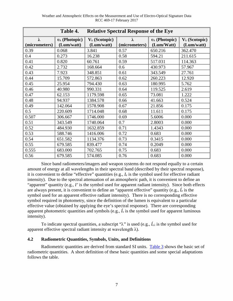
Table 4. Relative Spectral Response of the Eye λ
(micrometers) ʋλ (Photopic) (Lum/watt)
Vλ (Scotopic) (Lum/watt)
λ (micrometers)
ʋλ (Photopic) (Lum/Watt)
Vλ (Scotopic) (Lum/watt)
0.39 0.068 3.841 0.57 650.216 362.470 0.4 0.273 16.238 0.58 594.21 211.615 0.41 0.820 60.761 0.59 517.031 114.363 0.42 2.732 168.664 0.6 430.973 57.967 0.43 7.923 348.851 0.61 343.549 27.761 0.44 15.709 572.863 0.62 260.223 12.920 0.45 25.954 794.430 0.63 180.995 5.762 0.46 40.980 990.331 0.64 119.525 2.619 0.47 62.153 1179.598 0.65 73.081 1.222 0.48 94.937 1384.578 0.66 41.663 0.524 0.49 142.064 1578.908 0.67 21.856 0.175 0.5 220.609 1714.048 0.68 11.611 0.175 0.507 306.667 1746.000 0.69 5.6006 0.000 0.51 343.549 1740.064 0.7 2.8003 0.000 0.52 484.930 1632.859 0.71 1.4343 0.000 0.53 588.746 1416.006 0.72 0.683 0.000 0.54 651.582 1134.376 0.73 0.3415 0.000 0.55 679.585 839.477 0.74 0.2049 0.000 0.555 683.000 702.765 0.75 0.683 0.000 0.56 679.585 574.085 0.76 0.683 0.000
Since band radiometers/imagers and weapon systems do not respond equally to a certain amount of energy at all wavelengths in their spectral band (described by their spectral response), it is convenient to define “effective” quantities (e.g., Ie is the symbol used for effective radiant intensity). Due to the spectral attenuation of an atmospheric path, it is convenient to define an “apparent” quantity (e.g., I’ is the symbol used for apparent radiant intensity). Since both effects are always present, it is convenient to define an “apparent effective” quantity (e.g., Íe is the symbol used for an apparent effective radiant intensity). There is no corresponding effective symbol required in photometry, since the definition of the lumen is equivalent to a particular effective value (obtained by applying the eye’s spectral response). There are corresponding apparent photometric quantities and symbols (e.g., Ív is the symbol used for apparent luminous intensity).
To indicate spectral quantities, a subscript “λ” is used (e.g., Íeλ is the symbol used for apparent effective spectral radiant intensity at wavelength λ).
4.2 Radiometric Quantities, Symbols, Units, and Definitions Radiometric quantities are derived from standard SI units. Table 3 shows the basic set of
radiometric quantities. A short definition of these basic quantities and some special adaptations follows the table.

Weather and Atmospheric Effects on the Measurement and Use of Electro-Optical Signature Data RCC 469-17 February 2017
8
Source radiation is described by either radiant intensity (point sources) or radiance (extended sources). Both of these quantities generally vary with target aspect angle. Radiant intensity and radiance exist at the target and cannot be directly measured remotely.
The target radiation (described by either radiance or radiant intensity) propagates away from the target. The resulting radiation flux density at a remote point is described by an irradiance value. Target signatures must be derived from a measurement of irradiance.
Radiant energy (Q joules) is the energy (watt-sec) transferred by EO photons (within a specified spectral band) in a specified time period. It is the integral over time of radiant flux (watts). At a remote location, joules/meter2 (fluence) is the integral of irradiance (watts/meter2) over a specified time period.
∑∑ ∆=∆Φ=2
1
2
1
t
t
t
tAA tEAtQ 4.1
where: A is an area perpendicular to the beam
The output of integrating detectors is a function of the radiant energy transferred during their integration time. Radiant energy is often used to describe the output per pulse of short-pulse lasers (e.g., X joules/pulse).
Radiant flux (P or Φ watts) is the rate of transfer of radiant energy. It is sometimes called radiant power or radiant power flux. It is the radiant energy transferred per second.
4.2
The time-varying output of a non-integrating detector is a function of the time-varying radiant flux falling on the detector (assuming that the detector has an appropriate time constant).
Radiant power is commonly used to describe the output of continuous-wave lasers and to state the peak power of short-pulse lasers. A HEL might be specified as X megawatts (average power) and the peak power of a high-power laser designator might be specified as X megawatts (peak power). It is important to distinguish between a HEL and a high-power laser. A high-peak-power pulsed laser is not generally considered a HEL (e.g., a 100-megawatt peak power, 10-nanosecond pulse length, 10-pulse/second laser would have an average power of only 10 watts).
Irradiance (E watts/m2) describes the radiant power flux (Φ) per unit area at a point remote from a source. It is the only radiometric quantity that is observable remotely. Irradiance is produced by target radiance (L) and/or target radiant intensity (I), modified by path transmission (τ).
Radiation from all sources has a spectral distribution, described by spectral radiance (Lλ) or spectral radiant intensity (Iλ). Atmospheric path transmission (τλ) also varies with wavelength. As a result, the irradiance existing at a remote point has a certain spectral distribution (Eλ). The subscript λ is used to indicate a spectral quantity.
If there was no atmospheric attenuation (τλ=1.00) the spectral irradiance (Eλ) due to a target describable by spectral radiant intensity (Iλ) or by spectral radiance (Lλ) would be:

Weather and Atmospheric Effects on the Measurement and Use of Electro-Optical Signature Data RCC 469-17 February 2017
9
or
4.3
Atmospheric spectral transmission coefficients quantify the atmospheric transmission in small spectral bandwidths centered at a specified wavelength. Real atmospheric paths have spectral transmission coefficients less than 1 at all wavelengths and for all path lengths. Therefore, the spectral irradiance existing at a remote point must consider atmospheric path transmission as shown in Equation 4.4.
or 4.4
where: Eλ is the irradiance existing at observation point τλ is the path spectral transmission Íλ and Ĺλ are apparent spectral quantities The prime superscript indicates an apparent quantity
The apparent spectral radiant intensity or the apparent spectral radiance of a target (based on the observed spectral irradiance) is less than the actual values, since the atmosphere attenuates the spectral irradiance. A prime superscript is used to indicate an apparent radiant intensity or an apparent radiance value. Irradiance is not an apparent value (even though it is derived from apparent radiance or radiant intensity) and therefore does not have a prime superscript.
Spectral band irradiance is the integral of spectral irradiance values over a specified spectral band (λ1 to λ2) as shown in Equation 4.5. Summations are used since all of the spectral values involved are discrete. The indicated summations can be accomplished in a worksheet such as Microsoft Excel. It should be noted that the summation is slightly different from the integral, the amount of the difference depending on the spectral bandwidth (Δλ) involved. To compensate for this difference, the end points of the sum can be halved.
or
4.5
where: E is the actual band (λ1 to λ2) irradiance at observation point Í and Ĺ are apparent band radiant intensity and radiance, respectively ω is the instantaneous field of view (IFOV) of the observing system
Band measurement instruments must be calibrated in terms of effective irradiance (or effective radiance). Effective spectral irradiance is defined to be the product of the relative spectral response of the observing system (rλ) and the actual spectral irradiance (Eλ) arriving at the radiometer. Effective radiometric quantities are indicated by a subscript “e” (e.g., effective band irradiance is indicated by Ee and effective spectral irradiance is indicated by Eeλ). Since the actual spectral irradiance existing at a point is due to a target’s apparent spectral radiant intensity or apparent spectral radiance, effective spectral irradiance is calculated with Equation 4.6.

Weather and Atmospheric Effects on the Measurement and Use of Electro-Optical Signature Data RCC 469-17 February 2017
10
or
4.6
or
or
where: Eeλ is the effective spectral radiance at range R Ee is the measured effective band irradiance at range R Iλ is the target’s actual spectral radiant intensity Ieλ is the target’s effective spectral radiant intensity Leλ is the target’s effective spectral radiance Íeλ is the target’s apparent effective spectral radiant intensity at range R Ĺeλ is the target’s apparent effective spectral radiance at range R ω is the IFOV of the observing system
Not all of the irradiance arriving at remote points is due to a target of interest (additional irradiance may be due to background/foreground radiation or energy scattered toward the observation point). This additional irradiance must be removed from the measured data in order to obtain accurate target signature data. Observable band irradiance from real-world targets (and other sources) varies with spectral band, range, target aspect angle, and path transmission.
Radiance (L watts/steradian [sr]/m2) describes the radiation from an extended surface. Radiance is radiant intensity per unit (projected) surface area (in a defined spectral band and in a defined direction from the source) in the neighborhood of surface points. It is the quantity of choice to describe the spatial radiation from a target that over-fills the field of view (FOV) (ω steradians) of a system’s single detector (IFOV) viewing the surface. Radiance spatial distribution is measured with imaging radiometers.
The area to be considered in the definition of radiance is the projected surface area perpendicular to the viewing angle (line-of-sight to the observation point). For an arbitrary surface, radiance may vary in a complicated way with viewing angle. For a Lambertian surface, radiance is independent of viewing angle. Many radiators of military interest are near-Lambertian.
Radiance describes the spatial radiation from a source and, therefore, is not observable remotely. Radiance results in a measurable irradiance value at remote points and a measurement instrument can be calibrated in terms of either effective irradiance or apparent effective radiance. Either calibration process requires that calibration path spectral attenuation be determined and applied to the calibration source spectral distribution, since the instrument responds to the effective irradiance that actually exists at the measurement instrument. When each pixel of an imaging radiometer is calibrated in terms of apparent effective radiance or effective irradiance, the measurement of a target will result in apparent effective radiance spatial distribution data. It is apparent radiance since the irradiance at the radiometer has been reduced by atmospheric attenuation. It is effective radiance since the radiometer must be calibrated in terms of effective
Weather and Atmospheric Effects on the Measurement and Use of Electro-Optical Signature Data RCC 469-17 February 2017
11
quantities. The actual radiance signature of a target can be determined from measured apparent effective radiance data. The process is discussed in Section 5.
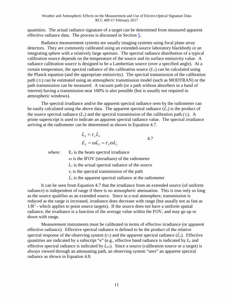
Radiance measurement systems are usually imaging systems using focal plane array detectors. They are commonly calibrated using an extended-source laboratory blackbody or an integrating sphere with a relatively large aperture. The spectral radiance distribution of a typical calibration source depends on the temperature of the source and its surface emissivity value. A radiance calibration source is designed to be a Lambertian source (over a specified angle). At a certain temperature, the spectral radiance of the calibration source (Lλ) can be calculated using the Planck equation (and the appropriate emissivity). The spectral transmission of the calibration path (τλ) can be estimated using an atmospheric transmission model (such as MODTRAN) or the path transmission can be measured. A vacuum path (or a path without absorbers in a band of interest) having a transmission near 100% is also possible (but is usually not required in atmospheric windows).
The spectral irradiance and/or the apparent spectral radiance seen by the radiometer can be easily calculated using the above data. The apparent spectral radiance (Ĺλ) is the product of the source spectral radiance (Lλ) and the spectral transmission of the calibration path (τλ). A prime superscript is used to indicate an apparent spectral radiance value. The spectral irradiance arriving at the radiometer can be determined as shown in Equation 4.7.
4.7
where: Eλ is the beam spectral irradiance ω is the IFOV (steradians) of the radiometer Lλ is the actual spectral radiance of the source τλ is the spectral transmission of the path Ĺλ is the apparent spectral radiance at the radiometer
It can be seen from Equation 4.7 that the irradiance from an extended source (of uniform radiance) is independent of range if there is no atmospheric attenuation. This is true only so long as the source qualifies as an extended source. Since in a real atmosphere, transmission is reduced as the range is increased, irradiance does decrease with range (but usually not as fast as 1/R2 - which applies to point source targets). If the source does not have a uniform spatial radiance, the irradiance is a function of the average value within the FOV, and may go up or down with range.
Measurement instruments must be calibrated in terms of effective irradiance (or apparent effective radiance). Effective spectral radiance is defined to be the product of the relative spectral response of the observing system (rλ) and the apparent spectral radiance (Ĺλ). Effective quantities are indicated by a subscript “e” (e.g., effective band radiance is indicated by Le and effective spectral radiance is indicated by Leλ). Since a source (calibration source or a target) is always viewed through an attenuating path, an observing system “sees” an apparent spectral radiance as shown in Equation 4.8.

Weather and Atmospheric Effects on the Measurement and Use of Electro-Optical Signature Data RCC 469-17 February 2017
12
since:
4.8 and:
where: Ĺeλ is the apparent effective spectral radiance
Ĺλ is the apparent spectral radiance Lλ is the actual spectral radiance of the source
is the normalized radiometer spectral response
ℜλ is the radiometer output per radiance value The calibration of an imaging radiometer consists of exposing the radiometer to a
uniform radiance calibration source that overfills the radiometer’s IFOV, accounting for the calibration path transmission, calculating the effective radiance, and recording the system’s output vs. effective radiance values. For many radiometers, the data plots as a straight line (describable by a slope and intercept).
A typical target is not likely to have the same radiance value at all points on its surface, to have the same angular distribution of radiance from each point, or to have the same spectral distribution from point to point. Calibration sources are designed to have a uniform spatial radiance and a known spectral distribution (at each temperature setting) over the radiating surface. Unless a target has a uniform radiance within a measurement instrument’s IFOV, the measurement will yield an average radiance value for that IFOV.
A band radiometer or a weapon system operating over a certain spectral band produces an output for each elemental detector representing an average apparent effective band radiance (Íe) within its IFOV. Band radiance is the spectrally integrated value of the spectral radiance over a spectral band of interest, as shown in Equation 4.9
4.9
where: L is the actual band radiance in IFOV (ω) Lλ is the actual spectral radiance in IFOV (ω) Ĺ is the apparent band radiance Ĺe is the apparent effective band radiance
Radiant intensity (I watts/sr) describes the total watts/sr radiated in a certain direction by a target that subtends a solid angle less than the IFOV of an observing system (in other words, a single detector element can “see” the entire target of interest). It is the quantity of choice for describing the radiation from such point source targets.

Weather and Atmospheric Effects on the Measurement and Use of Electro-Optical Signature Data RCC 469-17 February 2017
13
Radiant intensity is a property of a target. It cannot be measured remotely, but must be inferred from a measurement of irradiance at a remote point (R) from the target. Band radiant intensity is normally determined by measuring band irradiance using a radiometer or by using a spectral radiometer with a single detector having a relatively large field of regard (Ω). It can also be obtained from data collected with an imaging or scanning radiometer by summing target radiance data over the surface of the target.
Radiometers used to measure radiant intensity are normally calibrated in terms of effective irradiance using a cavity blackbody with small selectable apertures over the exit of the cavity, the source being placed at the focus of a collimating mirror. Desired irradiance values can be obtained by selecting an appropriate source temperature (which yields a certain source-relative spectral radiance distribution) and/or by selecting apertures of various sizes (which increase/decrease the amplitude of the radiant intensity distribution).
Band radiometers and weapon systems have a certain normalized spectral response (rλ). Calibration sources have a certain spectral radiance distribution (Lλ). Cavity blackbodies have apertures of known area (A). Collimators have certain spectral reflectance characteristics (ρλ). Calibration paths have certain spectral transmission coefficients (τλ). Using these values and the collimator parameters (focal length and spectral reflectivity), calibration effective irradiance values can be calculated. If actual irradiance values are used to calibrate a radiometer, the calibration data is different for different source radiance distributions (different source temperatures). If effective irradiance values are used to calibrate a radiometer, the calibration data is independent of source spectral distribution. Therefore, band radiometers used to measure point source targets are calibrated in terms of effective band irradiance (Ee). When a radiometer is calibrated in terms of effective band irradiance, measured target data will also be effective band irradiance and target radiant intensity data directly derived from the measured data (by using Íe=EeR2) will be the apparent effective radiant intensity. The measured data must be corrected to obtain desired actual target band radiant intensity data. The method required to make this correction will be discussed in Section 5.
If there was no atmospheric attenuation (τ =1), target radiant intensity data could be obtained directly from target irradiance data as shown in Equation 4.10.
4.10
where: Iλ is the target’s spectral radiant intensity Eλ is the resulting spectral irradiance at R E is the band irradiance in spectral band λ1 to λ2 ( )vac assumes a non-attenuating path
All radiometers (and weapon systems) have a relative spectral response (rλ) and the spectral transmission of the atmospheric path (τλ) is not 100%. The apparent spectral radiant intensity as seen by the radiometer is the product of the source spectral radiant intensity and the spectral transmission (τλ) of the measurement (or calibration) path. Apparent spectral radiant

Weather and Atmospheric Effects on the Measurement and Use of Electro-Optical Signature Data RCC 469-17 February 2017
14
intensity (and apparent band radiant intensity) values are less than what would exist for a non-attenuating path. The spectral and band irradiance for a real path are shown in Equation 4.11. A prime superscript is used to indicate an apparent value.
4.11
where: Iλ is the spectral radiant intensity of the source Íλ is the apparent spectral radiant intensity of the source τλ is the spectral transmission of the path Eλ is the spectral irradiance at the radiometer E is the band irradiance at the radiometer R is the distance to the observation point
Band radiometers are calibrated in terms of effective irradiance in order to produce a calibration that is independent of source spectral distribution. Effective spectral irradiance is defined to be the product of actual spectral irradiance (Eλ) and the relative spectral response (rλ) of the measurement instrument. A subscript “e” is used to indicate an effective radiometric value. Since measurements are made through an attenuating atmospheric path, raw irradiance measurements yield apparent effective radiant intensity values, as shown in Equation 4.12. A subscript “eλ” is used to indicate an effective spectral irradiance value.
4.12
where: Eeλ is the effective spectral irradiance at distance R Ee is the effective band irradiance in spectral band λ1 to λ2 Iλ is the actual spectral radiant intensity of the source Íλ is the apparent spectral radiant intensity of the source Íeλ is the apparent effective spectral radiant intensity of the source τλ is the atmospheric path transmission coefficient
is the normalized radiometer spectral response
ℜ is the radiometer output per radiant intensity value
System spectral responsivity (ℜλ and rλ) (system output [volts, digital counts, etc.] per unit of spectral irradiance [Eλ] or of apparent spectral radiance [Ĺλ]) describes the spectral response of a system, which is a function of the detector spectral response, filter spectral transmission, and the spectral transmission or reflectivity of the optical system used. It is

Weather and Atmospheric Effects on the Measurement and Use of Electro-Optical Signature Data RCC 469-17 February 2017
15
preferable that a system’s spectral response be measured for all measurement configurations, rather than trusting a calculation based on mathematically combining the spectral characteristics of individual system components. The normalized system spectral response (rλ) is the quantity most often needed in the process of correcting measured data for atmospheric effects. It is often easier to measure the relative system spectral response than to measure the absolute spectral response.
Quantum detectors are the most common type of detectors used in target measurement systems and in guided weapons. These detectors respond linearly to the number of incident photons in their band. Because short-wavelength photons carry a larger energy than do long-wavelength photons, spectral response (detector output per spectral irradiance value) increases with an increase in wavelength. Spectral filters can be used to make the response more uniform (but at the expense of increased signal-to-noise ratio [SNR]).
Thermal detectors typically have a uniform spectral response, but are generally not suitable for the low levels of irradiance produced by most military targets. Thermal detectors are most useful for high-radiance targets having slow time variation characteristics.
Spectral transmission characteristics quantify the spectral transmission of the atmosphere in small wavelength intervals (Δλ) at wavelengths (λ). These coefficients are usually calculated using an atmospheric transmission model (such as MODTRAN), although there are tables (see Wolfe3, for example) that provide a capability to estimate the coefficients for typical paths. The spectral transmission coefficients are required to calculate a correction factor to produce actual target signature data from measurements made through an atmospheric path. The primary atmospheric constituents that attenuate IR radiation are carbon dioxide (CO2), water vapor molecules (H2O), ozone (O3), and scattering aerosols. The primary atmospheric attenuators for UV radiation are O3, oxygen (O2), aerosols, and molecular scattering. The primary atmospheric attenuators for visible radiation are scattering aerosols (dust, smoke, haze, condensed water droplets, etc.).
Atmospheric path radiance between a target and a remote receiving system may increase the apparent radiance of a target. Radiance of the background within a radiometer’s FOV may affect the apparent radiant intensity of a target. The spectral distribution of path radiance is a function of the temperature along the path and the path emissivity (ελ), which is a function of path length. The temperature along typical atmospheric paths is low (below 300 K) and thus, path radiance is fairly low except at long-IR wavelengths (8-14 μm). Spectral emissivity is related to spectral absorption (αλ), (ελ=αλ). The primary long-IR wavelength absorbers in the atmosphere are CO2 (9-14 μm) and H2O (7-9 μm) molecules. Since water vapor in the atmosphere drops off very quickly with altitude and CO2 content decreases linearly with pressure, path radiance in the atmospheric windows is primarily a problem for long paths at low altitudes. Atmospheric models (such as MODTRAN) provide a method of estimating path radiance.
3 William L. Wolfe. The Infrared Handbook. Washington: Office of Naval Research, 1993.

Weather and Atmospheric Effects on the Measurement and Use of Electro-Optical Signature Data RCC 469-17 February 2017
16
4.3 Photometric Quantities, Symbols, Units, and Definitions Light is defined as that part of the electromagnetic spectrum that the human eye can see.
The wavelengths of light are between about 0.38 and 0.78 μm, although 0.4 to 0.7 μm are often used. Photometric quantities are used to describe light. All the units used in stating the various light quantities are based on the candela, which is an SI unit defining the luminous intensity from a point source in a certain direction. The candela replaced the quantity “candle power” in 1948, but the term candle power is still being used. A candlepower is approximately equal to 0.981 candela. Members of the RCC are encouraged to use the new quantities. The candela and other photometric quantities are defined in terms of the photopic (high light level) spectral response of the human eye (standard observer). The eye’s relative photopic luminous efficiency is shown in Figure 2. The photopic response is often called the “standard luminosity curve.”
Figure 2. Relative Spectral Response of the Eye
Table 4 lists the relative spectral response data plotted in Figure 2. The photopic response peaks at 0.555 μm with a value of 683 lumens per watt. The scotopic response peaks at 0.507 μm with a value of 1746 lumens per watt. It should be noted that the spectral responses listed are average responses. Some individuals may have a spectral response slightly different from the listed values.
Photometric quantities can be determined from radiometric quantities by weighting their radiometric spectral distribution with the relative spectral response of the eye. Photometric quantities are equivalent to effective radiometric quantities (defined earlier) where the system’s spectral response is the standard luminosity data. Photometric quantities (luminance, luminous intensity, and illuminance) can be obtained from band radiometric quantities by multiplying the
Photopic and Scotopic Spectral Responseof a Standard Observer
0
100
200
300
400
500
600
700
800
900
1000
1100
1200
1300
1400
1500
1600
1700
0.4 0.45 0.5 0.55 0.6 0.65 0.7
Wavelength (micrometers)
Res
pons
e (lu
men
s/w
att)
Scotopic (Low Light Level) Response
Photopic (Normal Light Level) Response

Weather and Atmospheric Effects on the Measurement and Use of Electro-Optical Signature Data RCC 469-17 February 2017
17
corresponding effective radiometric quantities (effective radiance, effective radiant intensity, and effective irradiance) by 683.
4.13
where: Φv is the luminous flux in band λ1 to λ2 Φλ is the spectral radiant flux vλΦλ is the effective spectral radiant flux vλ is the relative scotopic response of the eye Vλ is the absolute scotopic response (Table 4)
Table 5 lists a basic set of photometric quantities. A short definition of these quantities and some special adaptations follow the table.
Table 5. Basic Photometric Quantities, Symbols, and Units Photometric
Quantity Applies To Preferred Symbol Units*
Quantity Name
Luminous Energy
Effective Energy Unit
Qv Lumens-sec Talbot
Luminous Flux
Effective Power Unit
Φ v Lumens Lumen
Luminance Source of Flux Lv Lumens/sr/m2 Nit Luminous Intensity
Source of Flux Iv Lumens/sr Candela
Illuminance Received Flux Ev Lumens/m2 Lux *Centimeters are sometimes used as area units instead of meters.
There are other photometric quantities that may be encountered. Included are the foot-candle (lumens/ft2) and the Phot (lumens/cm2) illuminance quantities and stilb (candela/cm2) luminance quantity. There are other quantities that apply only to Lambertian sources, including apostilb (candela/m2/π), Lambert (candela/cm2/π), and foot-Lambert (candela/ft2). The RCC ranges are strongly encouraged to use the quantities listed in Table 5.
Illuminance (Eυ lumens/m2) describes the luminous flux (Φ) per unit area at a point remote from a source. It is the only photometric quantity observable remotely. Illuminance is produced by target luminance (Lυ) and/or target luminous intensity (Iυ), modified by path transmission (τ).
Radiation from all sources has a spectral distribution, described by spectral luminance (Lυλ) or spectral luminous intensity (Iυλ). Atmospheric path transmission also varies with wavelength (τλ). As a result, the illuminance existing at a remote point has a certain spectral distribution (Eυλ). The subscript v is used to indicate a photometric quantity. The subscript λ is used to indicate a spectral quantity.
If there was no atmospheric attenuation (τλ=1) the spectral illuminance (Eυλ) due to a target describable by spectral luminous intensity or by spectral luminance would be:

Weather and Atmospheric Effects on the Measurement and Use of Electro-Optical Signature Data RCC 469-17 February 2017
18
or 4.14
If there was no path attenuation
where: Evλ is the spectral illuminance (lumens/m2) at distance R ( )vac indicates 100% transmission (a vacuum) Ivλ is the spectral luminous intensity of the radiator Lvλ is the spectral luminance of the radiator R is the distance from the radiator ω is the IFOV of the receiving system
Since path spectral transmission is always less than unity at all wavelengths and for all path lengths (including calibration paths), the spectral illuminance at an observation point is less than that indicated above, and:
or
4.15
where: Evλ is the illuminance existing at observation point τλ is the path spectral transmission Ív and Ĺv are apparent spectral quantities The prime superscript indicates an apparent quantity
Spectral band illuminance is the integral (sum) of a target’s spectral illuminance over the visual spectral band (0.38 to 0.78 μm):
or
4.16
or
where: Ev is the actual band (λ1 to λ2) illuminance at observation point
Ív and Ĺv are apparent band luminous intensity and luminance τλ is the atmospheric spectral transmission coefficient
Photometers are calibrated in terms of either illuminance (Iυ) or apparent luminance (Ĺv=∑τλLvλ∆λ), where Lυλ is the spectral luminance of the calibration source (corrected for any optical components in the calibration path) and τλ are the atmospheric spectral transmission coefficients.
Calibration of photometers is usually accomplished by exposing the photometer to a standard luminance source (often an integrating sphere) or by placing a visible standard point source at the focus of a collimating mirror and placing the photometer in the collimated beam. When the point source method is used, the luminous intensity of the source (and thus the illuminance in the collimated beam) is usually accomplished by placing apertures of known size

Weather and Atmospheric Effects on the Measurement and Use of Electro-Optical Signature Data RCC 469-17 February 2017
19
over the source, although the luminance of the source can also be changed by controlling the calibration source current. The spectral transmission of the calibration path and the spectral reflection characteristics of the collimating mirror must be used to obtain the calibration illuminance values. Equation 4.17 can be used to calculate the calibration apparent band luminance and/or band illuminance values.
4.17
or
where: Ĺv is the apparent band luminance in the spectral band λ1 to λ2 ρλ is the spectral reflectivity value of the collimator (if used) τλ is the atmospheric spectral transmission coefficient Lvλ is the spectral luminance value of the calibration source Aα is the area of the source aperture ω is the IFOV of the imaging photometer f is the focal length of the collimating mirror
A high-temperature laboratory blackbody can be used to calibrate a photometer. The spectral radiance (Lλ) of the calibration source can be determined using the Planck equation (combined with the source emissivity). The apparent spectral radiance (Ĺλ) can be determined by applying the collimator spectral reflectance (ρλ) and the calibration path spectral transmission coefficients (τλ), which are usually near unity in the visible spectrum. The apparent spectral luminance is determined by applying the standard luminosity distribution. This process is illustrated in Equation 4.18.
4.18
where: Lλ is the spectral radiance (watts/sr/m2) of the blackbody Vλ is the absolute photopic response of the eye (Table 4) vλ is the relative photopic response of the eye (Table 4)
When a photometer is calibrated in terms of illuminance and used to determine the luminous intensity signature of a target through an attenuating path of length R, the resulting raw data is apparent luminous intensity values. The measured value must be corrected for the

Weather and Atmospheric Effects on the Measurement and Use of Electro-Optical Signature Data RCC 469-17 February 2017
20
atmospheric path attenuation to obtain an actual target luminous intensity value as shown in Equation 4.19.
4.19
where: Ív is the measured/calibrated band luminous intensity value Iv is the actual band luminous intensity value Ivλ is the actual spectral luminous intensity of the target ivλ is the normalized target spectral luminous intensity (Ivλ)max is the maximum spectral value of Ivλ
Luminance (Lv lumens/sr/meter2 = candela/meter2) describes the luminous intensity per unit area of a source of photometric flux. Luminance is the photometric term corresponding to the radiometric quantity effective radiance. Luminance describes the brightness (to the eye) of an extended surface. Luminance is luminous intensity per unit (projected) surface area (in a defined direction from the source) in the neighborhood of surface points. It is the quantity of choice to describe the spatial luminous flux from a target with sufficient angular size that it can be resolved by the eye (or a photometer).
The area to be considered in the definition of luminance is the projected surface area perpendicular to the viewing angle (line-of-sight to the observation point). For an arbitrary surface, luminance may vary in a complicated way with viewing angle. For a Lambertian surface, luminance is independent of viewing angle. Many sources of military interest are near-Lambertian.
Luminance describes the photometric characteristics of a source and, therefore, is not observable remotely. Luminance results in a measurable illuminance value at remote points and a measurement instrument can be calibrated in terms of either illuminance or apparent luminance. Either calibration process requires that calibration path spectral attenuation be determined and applied to the calibration source spectral distribution, since the instrument responds to the illuminance that actually exists at the measurement instrument. The transmission of a short calibration path in the visible portion of the spectrum is near unity, and therefore is generally ignored. When an imaging radiometer is calibrated in terms of apparent luminance or illuminance, the measurement of a target will result in apparent luminance data since the illuminance at the radiometer has been reduced by an existing atmospheric attenuation. The actual luminance signature of a target can be determined from measured apparent illuminance data. The process is discussed later in this paper.
Luminance measurement systems are often imaging systems using charge-coupled device array detectors. They are commonly calibrated using a standard extended luminance source (such as an integrating sphere). The spectral luminance distribution of a typical photometric calibration source can be set to a range of values (based on periodic standard lab calibration

Weather and Atmospheric Effects on the Measurement and Use of Electro-Optical Signature Data RCC 469-17 February 2017
21
data). The spectral transmission of the calibration path (τλ) can be estimated using an atmospheric transmission model (such as MODTRAN) or the path transmission can be measured. At visible wavelengths, calibration path attenuation can generally be ignored.
The spectral illuminance and/or the apparent spectral luminance seen by a radiometer can be easily calculated using the above data. The apparent spectral luminance is the product of the source spectral luminance and the spectral transmission of the measurement path. A prime superscript indicates an apparent spectral luminance value. The spectral illuminance arriving at a radiometer can be determined as follows.
4.20
where: ω is the IFOV (steradians) of the radiometer Lvλ is the actual target spectral luminance Ĺvλ is the apparent target spectral luminance τλ is the atmospheric path spectral transmission Evλ is the spectral illuminance at the observation point
Photometric instruments used to measure the band luminance spatial distribution of extended-source targets are generally calibrated in terms of apparent band luminance; however, they can be calibrated in terms of band illuminance. Spectral band luminance or illuminance can be computed by integrating (summing) the spectral values over the spectral band of interest as shown in Equation 4.21.
4.21
where: Lv is the actual luminance in IFOV (ω) Lvλ is the actual spectral luminance in IFOV (ω) Ĺv is the apparent band luminance τλ is the atmospheric spectral transmission coefficient Eʋ is the illuminance at the receiver ω is the FOV (steradians) of the receiver
A typical target is not likely to have the same band luminance value at all points on its surface or to have the same spectral distribution from point to point. Calibration sources are designed to have a uniform spatial luminance and a known spectral distribution (at each source setting) over their surface. Unless a target has a uniform luminance within a measurement instrument’s IFOV, the measurement will yield an average luminance value for that IFOV. Luminance measurement systems may not have the same resolution as the human eye (1 arc-minute = approximately 0.3 milliradians). Therefore, a measurement of a source having a very non-uniform spatial radiance may result in average radiance measurements that are different from that seen by the eye (or another photometer with a different IFOV).

Weather and Atmospheric Effects on the Measurement and Use of Electro-Optical Signature Data RCC 469-17 February 2017
22
A (non-spectral) photometer or a weapon system operating over a certain spectral band produces a single output (for each elemental detector) representing an apparent band luminance (Ív). Band luminance is the spectrally integrated value of the spectral luminance over a spectral band of interest. It should be noted that the summation is slightly different from the integral, the amount of the difference depending on the spectral bandwidth (Δλ) involved. To compensate for this difference, the end points of the sum should be halved.
Luminous Intensity (Iv) is in units of lumens per steradian, which is equal to candela. The candela is an SI base unit. All the other photometric units are based on the candela. It is the radiation, in a given direction, of a source that emits monochromatic radiation at a wavelength of 555 nm and that has a radiant intensity in that direction of 1/683 watt per steradian.
Luminous intensity describes the total lumens per steradian emanating in a certain direction by a target that subtends a solid angle less than or equal to the IFOV of the eye or of an observing system. In other words, a point source is defined to be so small that a single detector element can “see” the entire target of interest. Luminous intensity is the quantity of choice for describing the radiation from such point source targets and is a property of a target. It cannot be measured remotely, but must be inferred from a measurement of illuminance at a remote observation point (R). Luminous intensity is normally determined by measuring illuminance using a photometer or spectral photometer with a single detector having a relatively large field of regard (Ω). Luminous intensity can also be obtained from data collected with an imaging or scanning photometer by summing target luminance data over the surface of a target.
Photometers used to measure luminous intensity are normally calibrated in terms of illuminance using a point source luminous intensity standard. A relatively high-temperature cavity blackbody is sometimes used. The point source may be placed at the focus of a collimating mirror to produce a known illuminance level at the photometer. Desired illuminance values can be obtained by selecting an appropriate source setting (which yields a certain source-relative spectral luminous intensity distribution), using neutral density filters, and/or by selecting apertures of various size (which increase/decrease the amplitude of the luminous intensity distribution). As has been noted, calibrating the photometer in terms of illuminance is equivalent to calibrating a radiometer in terms of effective irradiance.
Photometers are filtered to obtain the normalized spectral response (vλ) of the human eye. Calibration sources have a certain spectral luminance distribution (Lv). If apertures are used, they have a known area (A). Calibration paths have certain spectral transmission coefficients (τλ=approximately 1). Using these values and the collimator parameters (focal length and spectral reflectivity), calibration illuminance values can be calculated. If there was no atmospheric attenuation (τλ=1), target radiant intensity data could be obtained directly from measured target irradiance data.
4.23
where: Ivλ is the target’s spectral luminous intensity Evλ is the resulting spectral illuminance at R

Weather and Atmospheric Effects on the Measurement and Use of Electro-Optical Signature Data RCC 469-17 February 2017
23
Ev is the band illuminance in spectral band λ1 to λ2 ( )vac assumes a non-attenuating path
The spectral transmission of calibration paths (τλ) is approximately 1. If the calibration path is long and the transmission is not unity, the apparent spectral luminous intensity at the radiometer is the product of the source spectral luminous intensity and the spectral transmission of the measurement (or calibration) path. Apparent spectral luminous intensity (and apparent band luminous intensity) values are less than what would exist for a non-attenuating path. A prime superscript is used to indicate an apparent value. For paths where there is some spectral attenuation, the band illuminance and band apparent luminance are as shown in Equation 4.24.
4.24
where: Ivλ is the spectral luminous intensity of the source Ívλ is the apparent spectral luminous intensity of the source τλ is the spectral transmission of the path Evλ is the spectral illuminance at range R Ev is the band illuminance at the radiometer
Atmospheric Correction of Measured Target Signature Data and Applying Atmospheric Effects when using Target Signature Data
Target signature data obtained from remote measurements are affected by the atmosphere. For high-temperature targets, the primary effect is atmospheric attenuation. For low-temperature targets at longer wavelengths, both atmospheric attenuation and atmospheric path radiance affect the measurement. The atmospheric effects must be removed in order to obtain actual target signatures. When using target signature data to estimate weapon system performance, atmospheric effects for the scenario being considered must be applied to obtain the weapon system’s output signal and SNR.
Figure 3 illustrates the steps that are necessary to correct measured radiometric data for atmospheric effects and to use target signature data to estimate weapon system performance.

Weather and Atmospheric Effects on the Measurement and Use of Electro-Optical Signature Data RCC 469-17 February 2017
24
Figure 3. Atmospheric Correction Process
5.1 Atmospheric Correction of Target Data Collected with a Radiometer or Imaging Radiometer Effective irradiance or apparent effective radiance must be used to calibrate a radiometer
(or imaging radiometer). Effective values are the only quantities that will produce a unique set of calibration data (volts, counts, etc. vs. received band radiation) when using radiometers or imaging radiometers operating over a defined spectral band. Actual irradiance (or radiance) cannot be used because different calibration curves will be produced for different calibration source spectral distributions. For instance, using different blackbody temperatures will result in different calibration curves if actual irradiance (or apparent radiance) is plotted against system output. If effective values are plotted against system output, a single calibration curve will be produced, independent of the calibration source spectral distribution. Such a calibration can be used to determine the effective radiant intensity or effective radiance of targets, regardless of the target’s spectral radiation characteristics. The spectral response of a particular weapon system seeker is often different from the spectral response of the radiometer used to collect data being used. Therefore, the effective irradiance or effective radiance for the weapon system is different from the measured effective irradiance. The effective irradiance or apparent effective radiance for a particular weapon system can be computed from measured/ corrected signature data by applying the weapon system’s spectral response and operational path spectral transmission data.
All remote measurements are made through an attenuating atmosphere. The atmospheric spectral transmission coefficients (τλ), which have values from zero to one, are less than one for all measurement paths (including calibration paths). The atmospheric path, therefore, reduces

Weather and Atmospheric Effects on the Measurement and Use of Electro-Optical Signature Data RCC 469-17 February 2017
25
the observed irradiance and/or results in an observed radiance (called the apparent radiance) or an observed radiant intensity (called the apparent radiant intensity) that is less than what would exist through a non-attenuating path. The spectral irradiance existing at a distance R from a point source and from an extended source is shown in Equation 5.1.
or
5.1
where: Eλ is the spectral irradiance at the measurement location Iλ is the spectral radiant intensity of a point source Lλ is the spectral radiance of an extended source τλ is the spectral atmospheric transmission coefficient R is the distance between point source and radiometer ω is the IFOV (steradians) of the radiometer Íλ is the apparent radiant intensity of the point source Ĺλ is the apparent radiance of the extended source
Effective spectral irradiance (Eeλ) or effective spectral radiance (Leλ) is defined to be the product of the spectral irradiance (Eλ) or spectral radiance (Lλ) and the normalized spectral response of the radiometer (rλ). As noted earlier, band radiometers must be calibrated in terms of effective values. The prime superscript indicates an apparent value (a reduced value due to atmospheric attenuation). The subscript “e” indicates an effective value (a measure of the observing system’s capability to produce system output).
5.2
where: rλ is the normalized system spectral response Eλ is the spectral irradiance at range R Eeλ is the effective spectral irradiance Iλ is the actual spectral radiant intensity Íλ is the apparent spectral radiant intensity Íeλ is the apparent effective spectral radiant intensity Lλ is the actual target radiance Ĺλ is the apparent spectral radiance Ĺeλ is the apparent effective spectral radiance

Weather and Atmospheric Effects on the Measurement and Use of Electro-Optical Signature Data RCC 469-17 February 2017
26
Íe is the apparent effective band radiant intensity Ĺe is the apparent effective band radiance ω is the IFOV (steradians) of the radiometer
The effective band irradiance (Ee) or apparent effective band radiance (Ĺe) is obtained by summing the effective spectral quantities over the spectral band of a device.
5.3
When the effective values (either Ee or Ĺe) are plotted against system output (volts or digital counts) a unique (independent of source spectral distribution) calibration curve is obtained. The calibration curve will typically be linear and describable by a slope and an intercept.
A measuring instrument calibrated in terms of effective irradiance or apparent effective radiance, making measurements through an atmospheric path, will produce apparent effective target radiant intensity or apparent effective target radiance, rather than actual target radiance or radiant intensity. Actual target radiant intensity or radiance are the desired target signature data. In order to obtain the actual target signature data, the apparent effective values must be converted to actual values. The method required to accomplish this conversion is shown in the following paragraphs.
Target radiation data is usually reported as radiant intensity (I or J watts/sr) or radiance (L or N watts/sr/m2) although the remote measurement instrument’s output depends on the irradiance (E or H watts/m2) existing at the radiometer. Since radiometers are calibrated in terms of effective values and always make measurements through an attenuating path, the measured target data represents apparent effective values.
The apparent effective radiant intensity of a target measured with a system having a certain spectral band-pass, calibrated in terms of effective irradiance, and with the measurement made through at attenuating atmosphere is:
5.4
where: Iλ is the spectral radiant intensity of the target
is the normalized target spectral radiant density
rλ is the radiometer spectral response value τλ is the atmospheric transmission coefficient Ee is the measured band irradiance at range R

Weather and Atmospheric Effects on the Measurement and Use of Electro-Optical Signature Data RCC 469-17 February 2017
27
The actual band radiant intensity (the desired target radiant intensity signature) of a target within the spectral band of the radiometer is:
5.5
Therefore, the correction factor that must be applied to obtain actual target radiant intensity signature (I) from a measurement that produces apparent effective radiant intensity (Íe=EeR2) data is shown in square brackets in the equation below. For those who prefer the older symbols (J and H), that equation is shown on the right.
5.6
where: I (or J) is the desired actual target band radiant intensity
Ee (or He) is the measured target band effective irradiance
iλ, jλ, rλ, τλ are normalized spectral values of target radiant intensity, system specrtral response, and atmospheric transmission
In a similar manner, one can obtain the correction factor for obtaining a target’s radiance signature from measured apparent effective radiance data. Again the equations using the older symbols (N and H) are shown on the right below.
or
5.7
where: L (or N) is the actual target band radiance Ĺe (or Ńe) is the measured target band apparent effective radiance Ee (or He) is the measured target band effective irradiance lλ, nλ, rλ, or τλ are normalized spectral values of target radiance, system
spectral response, and atmospheric transmission
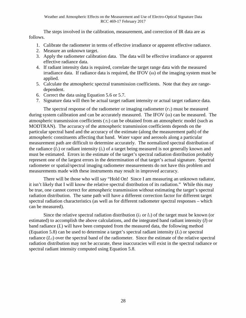
Weather and Atmospheric Effects on the Measurement and Use of Electro-Optical Signature Data RCC 469-17 February 2017
28
The steps involved in the calibration, measurement, and correction of IR data are as follows.
1. Calibrate the radiometer in terms of effective irradiance or apparent effective radiance. 2. Measure an unknown target. 3. Apply the radiometer calibration data. The data will be effective irradiance or apparent
effective radiance data. 4. If radiant intensity data is required, correlate the target range data with the measured
irradiance data. If radiance data is required, the IFOV (ω) of the imaging system must be applied.
5. Calculate the atmospheric spectral transmission coefficients. Note that they are range-dependent.
6. Correct the data using Equation 5.6 or 5.7. 7. Signature data will then be actual target radiant intensity or actual target radiance data.
The spectral response of the radiometer or imaging radiometer (rλ) must be measured during system calibration and can be accurately measured. The IFOV (ω) can be measured. The atmospheric transmission coefficients (τλ) can be obtained from an atmospheric model (such as MODTRAN). The accuracy of the atmospheric transmission coefficients depends on the particular spectral band and the accuracy of the estimate (along the measurement path) of the atmospheric constituents affecting that band. Water vapor and aerosols along a particular measurement path are difficult to determine accurately. The normalized spectral distribution of the radiance (lλ) or radiant intensity (iλ) of a target being measured is not generally known and must be estimated. Errors in the estimate of the target’s spectral radiation distribution probably represent one of the largest errors in the determination of that target’s actual signature. Spectral radiometer or spatial/spectral imaging radiometer measurements do not have this problem and measurements made with these instruments may result in improved accuracy.
There will be those who will say “Hold On! Since I am measuring an unknown radiator, it isn’t likely that I will know the relative spectral distribution of its radiation.” While this may be true, one cannot correct for atmospheric transmission without estimating the target’s spectral radiation distribution. The same path will have a different correction factor for different target spectral radiation characteristics (as well as for different radiometer spectral responses – which can be measured).
Since the relative spectral radiation distribution (iλ or lλ) of the target must be known (or estimated) to accomplish the above calculations, and the integrated band radiant intensity (I) or band radiance (L) will have been computed from the measured data, the following method (Equation 5.8) can be used to determine a target’s spectral radiant intensity (Iλ) or spectral radiance (Lλ) over the spectral band of the radiometer. Since the estimate of the relative spectral radiation distribution may not be accurate, these inaccuracies will exist in the spectral radiance or spectral radiant intensity computed using Equation 5.8.
Weather and Atmospheric Effects on the Measurement and Use of Electro-Optical Signature Data RCC 469-17 February 2017
29
5.8
where: I or L are the band values determined from the measured/corrected data iλ or lλ are the estimated target normalized spectral distribution Iλ or Lλ are the spectral radiant intensity or spectral radiance distribution
When comparing radiant intensity or radiance data measured using several instruments (perhaps used side by side), the only quantity that can be meaningfully compared is the actual target radiant intensity or radiance values. This requires that each set of measured data be accurately corrected before comparisons are made. Unless the atmospheric transmission coefficients and the spectral radiation characteristics of the target are accurately known, one should not expect exceptional correlation of the data produced by the various radiometers. If a source of known spectral characteristics is used in the comparison, the main source of concern will be the atmospheric transmission coefficients. If an actual real-world target is used, its spectral radiation characteristics should be measured and applied, if possible.
Many targets of military interest have a wide range of spectral radiance for different areas on the target (e.g., jet engine tailpipe, exhaust plume, skin radiation, etc.). Since different imager pixels will see different target spectral radiance values, applying the above correction equations is computationally intensive and require estimates of the spectral characteristics for the various target areas.
Even for radiant intensity measurements, the fact that different areas of a target have different spectral radiation distributions and the fact that different areas are likely to have different aspect angle dependence make the estimation of the required spectral radiant intensity distribution difficult.
In certain situations, the correcting of measured data to obtain actual target signature data (Equations 5.6 and 5.7) can be simplified. For instance, if the atmospheric spectral attenuation is fairly constant in the measurement band (which it often is in the atmospheric windows), it can be removed from the summation. If the spectral response of the measurement instrument is fairly constant (rλ ≈ 1), it can be removed from the summation. If these two situations exist, Equations 5.6 and 5.7 become as shown in Equation 5.9.

Weather and Atmospheric Effects on the Measurement and Use of Electro-Optical Signature Data RCC 469-17 February 2017
30
5.9
The spectral response (output per irradiance unit) of quantum detectors (the most common type) is not constant; however, the selection of an appropriate filter can make the spectral response of a measurement instrument relatively constant (at the expense of reduced irradiance responsivity at longer wavelengths). Thermal detectors typically have a relatively constant spectral response.
Another situation where Equations 5.6 and 5.7 can be simplified is when the atmospheric transmission is fairly constant over the band of interest (which is often the case in the atmospheric windows), but the spectral response of the receiving device is not independent of wavelength.
It can be seen from Equation 5.10 that the derivation of actual target signatures from measured effective irradiance requires the spectral distribution of the radiator, even if there is no atmospheric attenuation. If the spectral distribution of the target cannot be estimated and the atmospheric attenuation is relatively constant over the band of interest, an alternative is to report the effective values.
Measured signature data is sometimes reported as apparent effective radiance or apparent effective radiant intensity (Equation 5.11), where the measurements are not corrected for atmospheric attenuation or for radiometer spectral response. In this case, it is very important that the spectral response of the radiometer and sufficient weather data be reported to allow atmospheric corrections by customers (who then have the burden of estimating the spectral radiation characteristics of the target and correcting the measured data). Apparent effective radiant intensity or apparent effective radiance is obtained directly from a measurement of effective irradiance and range to the target.
5.10

Weather and Atmospheric Effects on the Measurement and Use of Electro-Optical Signature Data RCC 469-17 February 2017
31
5.11
where: Ee is the raw data with calibration applied
Whether any of the above assumptions are appropriate depends on the spectral transmission of the atmospheric path. The mid-wave IR band is a particular problem. The mid-wave IR band (3-5 μm) includes a strong CO2 absorption band (see Figure 4 and Figure 5). If a measurement band includes this absorption band, the assumption of a constant spectral transmission is invalid. If the band is 3.5-4.1 μm, the assumption may be valid. Carbon-based fuels produce a large percentage of their energy in this CO2 absorption band. A large portion of this radiation is absorbed by CO2 (even over fairly short paths); however, the spectral bandwidth of this absorption band varies (and thus the attenuation increases) with altitude and path length. There is CO2 at all locations and at all altitudes in a mixing ratio of approximately 330-400 parts per million, although it may be higher in an area due to local CO2 generation/absorption. Except for these local effects, the percentage of CO2 in the atmosphere at all locations and at all altitudes is about the same.
Figure 4. H20 Transmission

Weather and Atmospheric Effects on the Measurement and Use of Electro-Optical Signature Data RCC 469-17 February 2017
32
Figure 5. CO2 Transmission
Richards & Johnson measured the apparent 3-5-μm band radiance of a 100 °C extended-source blackbody at various ranges and calculated the spectral transmission over each path (using MODTRAN). This data illustrates the correction factor needed to obtain actual target radiance from measured apparent target radiance for a 100 °C blackbody. The combustion of any carbon-based fuel radiates a significant portion of its energy in the CO2 absorption band and the radiance (or radiant intensity) correction factors for these radiators would drop off even more dramatically with increasing range. A MODTRAN calculation of the transmission in the measurement paths is shown in Figure 6. The Richards & Johnson is shown in Figure 7. The relative spectral distribution of a 100 °C blackbody is shown in Figure 8 for reference.

Weather and Atmospheric Effects on the Measurement and Use of Electro-Optical Signature Data RCC 469-17 February 2017
33
Figure 6. Spectral Transmission of Measurement Paths
Figure 7. Relative Apparent Radiance vs. Range (100 °C BB)
0
0.1
0.2
0.3
0.4
0.5
0.6
0.7
0.8
0.9
1
3.5 3.6 3.7 3.8 3.9 4 4.1 4.2 4.3 4.4 4.5 4.6 4.7 4.8 4.9 5
Wavelength (micrometers)
Tran
smis
sion
5 Meter Path
200 Meter Path
1 Kilometer Path
Path Short Long Width m 1/2 1/2 (microns) 5 4.204 4.327 .123200 4.183 4.446 .2581000 4.182 4.540 .358
0.5
0.55
0.6
0.65
0.7
0.75
0.8
0.85
0.9
0.95
1
0 100 200 300 400 500 600 700 800
Range (meters)
Rel
ativ
e R
adia
nce

Weather and Atmospheric Effects on the Measurement and Use of Electro-Optical Signature Data RCC 469-17 February 2017
34
Figure 8. Relative Spectral Distribution (100 °C BB)
Note that the width of the CO2 absorption band increases as the path length is increased. A laboratory calibration path may have a small transmission in the band, but much of a target’s radiation in this band will not be measured. If the absorption band is included in a measurement band, correcting for atmospheric attenuation is problematic. If a higher-temperature blackbody had been used in the Richards & Johnson measurements, a different reduction in apparent radiance would be seen in Figure 7.
One way to avoid the complications (and some of the errors associated with correcting data collected with a band measurement instrument) is to use a spectral measurement instrument. Spectral radiometers and spectral imagers do not need to be calibrated using effective irradiance (or effective radiance). Calibration of spectral measurement systems consists of determining a set of outputs produced by a range of known spectral irradiance (or radiance) values at closely spaced wavelengths (λ) having narrow spectral bandwidths (∆λ).
Typically, the calibration source for a spectral radiometer includes a variable-temperature blackbody with variable apertures and a collimating mirror. Using the spectral reflection characteristics of the mirror and the spectral transmission characteristics of the calibration path, the spectral irradiance values at the spectral radiometer can be calculated. The set of spectral irradiance values and the corresponding spectral outputs (volts of digital counts) constitute the calibration data. By changing the temperature and/or the aperture area to produce a range of spectral irradiance values, a complete set of calibration data can be produced. If the input/output relationship is known to be linear, a single calibration point (and a determination of the radiometer noise level) may be sufficient to establish the calibration curve.
The calibration source for a spectral imaging radiometer is typically a variable-temperature extended-source blackbody with or without a collimating mirror. The extended-source blackbody might be a cavity blackbody or integrating sphere with a large aperture or a flat-surface extended source. To obtain a range of spectral radiance values, the temperature of the calibration source can be set to a range of values. The spectral reflectance of the collimator
0.0
0.1
0.2
0.3
0.4
0.5
0.6
0.7
0.8
0.9
1.0
3 3.5 4 4.5 5
Wavelength (micrometers)
Rel
ativ
e Sp
ectr
al R
adia
nce
Weather and Atmospheric Effects on the Measurement and Use of Electro-Optical Signature Data RCC 469-17 February 2017
35
and the calibration path spectral transmission coefficients can be applied to determine the apparent spectral radiance at the imager being calibrated. To accomplish an accurate calibration, it is important that the spectral emissivity of the source, the spectral reflectivity of the collimating mirror4, and the calibration path spectral transmission coefficients be accurately determined.
Spectral radiometers and imagers are, therefore, calibrated in terms of actual spectral irradiance or apparent spectral radiance respectively. When these instruments are used to measure a target through an attenuating atmosphere, the measured values can be corrected for atmospheric attenuation wavelength-by-wavelength and integrated to obtain actual band radiant intensity or actual band radiance. See Equation 5.12.
or
5.12
where: Eλ and Ĺλ are measured spectral irradiance and apparent spectral radiance I and L are the band radiant intensity and band radiance τλ is the atmospheric spectral transmission coefficient R is the distance to the observation point ω is the IFOV of the spectral radiometer
If a measuring instrument is accurately calibrated, measured spectral irradiance (Eλ) or apparent spectral radiance (Ĺλ) should be accurate. The measurement of the distance (R) should be accurate. The primary errors in the determination of actual target spectral radiant intensity (Iλ) or spectral radiance (Lλ) are in the estimates of the atmospheric transmission coefficients (τλ), which can be obtained from an atmospheric model (such as MODTRAN). The accuracy of these coefficients depends on the spectral wavelength and the accuracy of the estimate (along the measurement path) of the atmospheric constituents affecting that wavelength. The amount of water vapor and scattering aerosols along a measurement path are difficult to determine accurately.
Calculations using the above equations can easily be made using any one of several spreadsheet programs (such as Microsoft Excel) or using special software written to accomplish the calculations. If a canned data reduction package is used to accomplish the calculations, one should assure that the program accomplishes the calculations as specified in the above equations (or an equivalent validated method).
Users (such as modeling & simulation users) of measured/corrected target radiant intensity or radiance data must apply their particular system’s spectral response and the spectral transmission coefficients of their assumed path to determine the irradiance for their situation. They need to have actual target spectral radiance/luminance distributions or actual target spectral radiant intensity/luminous intensity data (as a function of target aspect angle). If such data is not provided, users must derive the needed data from the reported measurement data. Using their system spectral response data, computed transmission for their path, and target spectral radiant 4 Christopher Dobbins. “Measuring Collimator Infrared (IR) Spectral Transmission.” Technical Report RDMR-WD-16-15. May 2016. Retrieved 16 December 2016. Available at http://www.dtic.mil/get-tr-doc/pdf?AD=AD1009521.

Weather and Atmospheric Effects on the Measurement and Use of Electro-Optical Signature Data RCC 469-17 February 2017
36
intensity or spectral radiance data, the resulting system output and system SNR for their atmospheric path can be determined. The calculations can only be made for a weapon system spectral band that is within (equal to or less than) the spectral band of the measured/ corrected data. The weapon system calculations can be accomplished as follows, assuming that the target measurement and correction process have produced the spectral radiant intensity (Iλ) or spectral radiance (Lλ) of a target over the spectral band-pass of the radiometer,.
or
5.13
where: (ℜE)λ and (ℜL)λ are the weapon system’s absolute spectral responses
Iλ or Lλ are the measured (and corrected) target spectral distributions λ is the calculated spectral transmission value of the path R is the path length ω is the system IFOV
The SNR and system parameters resulting from it can be calculated using the outputs calculated above and the system noise level.
5.2 Atmospheric Correction of Target Data Collected with a Photometer or Imaging Photometer Band radiometric measurements are made with radiometers having a large variety of
spectral responses. Photometers have only one spectral response (the spectral response of the human eye). There is therefore only one effective photometric value. This effective value is called lumens. Other photometric quantities are related to this effective value (e.g., lumens/m2 [Ev], lumens/sr/m2 [Lv], and lumens/sr [Iv]).
Photometric data is usually reported as either source luminous intensity (Iv) or as a luminance (Lv) spatial distribution, although the remote instrument’s output depends on the illuminance (Ev) produced by the source at remote range R.
If there was no atmospheric attenuation, the actual target luminous intensity or luminance could be determined from Equation 5.14.
or
5.14
or
where: (Evλ)vac is the measurable spectral illuminance
Ivλ is the actual source luminous intensity

Weather and Atmospheric Effects on the Measurement and Use of Electro-Optical Signature Data RCC 469-17 February 2017
37
Lvλ is the actual source luminance R is the distance from source to observation point ω is the IFOV of the observing instrument
Since remote systems must always view targets through an attenuating path, the spectral illuminance will be reduced and a luminance or luminous intensity value derived from the reduced illuminance will yield an apparent luminance or apparent luminous intensity as shown in Equation 5.15.
or
5.15
or
where: Evλ is the measurable spectral illuminance at range R
Ivλ is the actual source spectral luminous intensity ivλ is the normalized distribution of Ivλ Ívλ is the apparent source spectral luminous intensity Ív is the apparent band luminous intensity Lvλ is the actual source spectral luminance lvλ is the normalized distribution of Lvλ Ĺvλ is the apparent source spectral luminance Ĺv is the apparent band luminance τλ is the spectral transmission of the atmospheric path ω is the IFOV of the observing instrument
The actual band luminous intensity of a target within the spectral band of the photometer (the desired target radiant intensity signature) is:
5.16
where: Iv is the band luminous intensity Ivλ is the spectral luminous intensity value (Ivλ)max is the maximum spectral luminous intensity
is the normalized spectral luminous intensity
Therefore, the correction factor that must be applied to obtain actual target luminous intensity signature (Iv) from a measurement that produces apparent luminous intensity (Ív) data is shown in square brackets in Equation 5.17.
Weather and Atmospheric Effects on the Measurement and Use of Electro-Optical Signature Data RCC 469-17 February 2017
38
5.17
where: Iv is the desired actual target band luminous intensity Ív is the measured target apparent band luminous intensity Ev is the measured target band effective illuminance ivλ is the normalized spectral value of the target luminous intensity τλ is the atmospheric spectral transmission coefficient
In a similar manner, one can obtain the correction factor for obtaining a target’s luminance signature from measured apparent luminance or illuminance data.
5.18
where: Lv is the actual target band luminance Ĺv is the measured target band apparent luminance Ev is the measured target band effective irradiance lvλ is the normalized spectral values of target luminance τλ is the atmospheric spectral transmission coefficients
The steps involved in the calibration, measurement, and correction of photometric data are as follows.
1. Calibrate the photometer in terms of illuminance or apparent luminance. 2. Measure an unknown target. 3. Apply the photometer calibration data. The data will be illuminance or apparent
luminance data. 4. If luminous intensity data is required, correlate the target range data with the measured
illuminance data. If luminance data is required, determine the IFOV of the imaging photometer.
5. Calculate the atmospheric spectral transmission coefficients. Note that they are range-dependent.
6. Correct the data using Equation 5.17 or Equation 5.18. 7. Signature data will then be actual target luminous intensity or actual target luminance
data.
The spectral response of the photometer or imaging photometer should be measured during system calibration to determine that it accurately represents the standard luminosity curve. The atmospheric transmission coefficients (τλ) can be obtained from an atmospheric

Weather and Atmospheric Effects on the Measurement and Use of Electro-Optical Signature Data RCC 469-17 February 2017
39
model (such as MODTRAN). The accuracy of the atmospheric transmission coefficients depends on the accuracy of the estimate of the atmospheric constituents along the measurement path. Aerosol scattering is often the primary constituent affecting visual transmission. Aerosols along a measurement path are difficult to determine accurately. The spectral distribution of the luminance (lvλ) or luminous intensity (ivλ) of a target being measured is not generally known and must often be estimated. Errors in the estimate of the target’s spectral distribution probably represent one of the largest errors in the determination of that target’s signature. Spectral photometers or spatial/spectral imaging photometers do not have this problem and measurements made with these instruments may result in improved accuracy.
Weather/Atmospheric Effects on Electro-Optical Systems Remote observations of targets are affected by atmospheric constituents along the
observation path. Some of these constituents can attenuate EO energy by absorption or scattering. Some may add EO energy by self-radiation or scattering of energy from other sources (primarily the sun). Weather can also present a complicated background clutter situation, making it difficult to isolate a target’s signature.
The earth’s atmosphere can be divided into several distinct layers. The lower layers are of most concern in military operations. These layers are depicted in Figure 9. Except for very high-flying aircraft and missiles, most military operations take place within the troposphere.
Figure 9. Lower Layers of the Earth’s Atmosphere
The troposphere extends from the surface of the earth up to altitudes of about 30,000 to 60,000 feet, depending on the latitude. It extends to the higher altitude over the equator and to the lower altitude at the poles. The temperature in the troposphere steadily drops about 3.6 °F per thousand feet of altitude (about 6.5 °C per kilometer). The temperature at the top of the
Mesosphere and Ionosphere
Stratosphere
Troposphere
Ozone LayerApprox. 70K-160K Feet
approx. 60K Feet
Approx. 200K Feet
Mesosphere and Ionosphere
Stratosphere
Troposphere
Ozone LayerApprox. 70K-160K Feet
approx. 60K Feet
Approx. 200K Feet

Weather and Atmospheric Effects on the Measurement and Use of Electro-Optical Signature Data RCC 469-17 February 2017
40
troposphere is about −70 °F (−57 °C). Warmer air near the surface rises (since its density is less than the cooler air above). The rising air cools and also displaces the upper air, causing the upper air to descend in the troposphere. This constant motion of the air in the troposphere produces wind, clouds, rain, and constantly changing weather conditions. Almost all weather takes place within the troposphere.
The stratosphere is a layer above the troposphere extending to approximately 300,000 feet. The O3 layer lies within the stratosphere and strongly absorbs some UV wavelengths, making it important to UV observations within the troposphere. Solar radiation is almost totally absorbed at these wavelengths (called “solar blind region”), allowing systems operating in the troposphere to detect very low radiation level targets (since there is no competing solar radiation – it is always dark at these wavelengths).
The lower part of the stratosphere is characterized by having a constant temperature (around −65 °F) called the tropopause. Toward the top of the stratosphere, the temperature rises as the altitude increases.
The earth’s lower atmosphere consists of a mixture of the so-called permanent constituents of the atmosphere and some variable constituents.
The permanent constituents of the atmosphere exist in constant proportion at all locations and at all altitudes. At the same pressure (altitude above mean sea level), the effect of the permanent constituents on EO systems is virtually the same at all test ranges. Since pressure decreases with altitude, the amount of these permanent constituents encountered (and therefore the effect along a certain path length) decreases with altitude. The composition of the permanent constituents (sometimes called dry air) is shown in Table 6.
Table 6. Constituents of Earth’s Atmosphere Constituent Symbol % by Volume Constituent Symbol % by Volume
Nitrogen N2 78.08 Methane CH4 0.0002 Oxygen O2 20.95 Krypton Kr 0.00011 Argon A 0.93 Nitrous Oxide NO 0.00005 Carbon Dioxide CO2 >0.033 Hydrogen H2 0.00005 Neon Ne 0.0018 Ozone (Summer) O3 0.000007 Helium He 0.00052 Ozone (Winter) O3 0.000002
Molecules have the capability to absorb and emit EO energy; however, less than 1% of the permanent atmospheric molecules absorb or emit EO energy, the primary absorbers being CO2 and O3 molecules. Of course, water vapor molecules also are primary absorbers, but water molecules are not a permanent part of the atmosphere.
Most (over 99%) of the permanent atmospheric constituents have negligible effect on the operation of EO systems. The primary effect is from CO2, even though it exists in the atmosphere at only 330 to 400 parts/million (may be higher near sources of CO2, such as industrial areas). One strong absorber of EO energy in the UV portion of the spectrum is O3, but most of it in the atmospheric exists in the O3 layer at altitudes above 70,000 feet. Methane and nitrous oxide have a very slight effect, but these molecules exist in the atmosphere at such low levels that they can basically be ignored. Of the variable constituents in the atmosphere, water molecules (whose amount can vary from near zero to about 4%) have the greatest effect on EO

Weather and Atmospheric Effects on the Measurement and Use of Electro-Optical Signature Data RCC 469-17 February 2017
41
systems (particularly the IR portion of the EO spectrum). Most of the water molecules are at low altitudes, the amount decreasing rapidly with increasing altitude. At altitudes above 30,000 feet, one can generally ignore the effects of water molecules. Since the humidity varies a lot from one test range to another, the effect on the performance of weapon systems (and on signature measurements) operating through low-altitude paths may be quite different at different locations.
While O3 has its primary effect on relatively long UV paths, there is not very much of it in the troposphere (the amount of O3 along a path varies with location and season). Tropospheric O3 has a negligible effect on visible and IR wavelengths.
All atmospheric molecules can scatter EO energy, but molecular scattering is only a factor at UV and short visible wavelengths. Other variable constituents in the atmosphere include dust, smoke, carbon exhaust particles, smog, haze, industrial pollutants, salt water droplets, fog, ice crystals, and clouds. These systems of small particles, suspended in the air are called “the aerosol”. Weather effects such as rain and snow have transient effects on EO systems. Figure 10 shows the transmission of a typical atmospheric path (about 1 nautical mile) at a low altitude. The atmospheric molecules responsible for reduced transmission are also shown.
Figure 10. Molecular Absorption at Electro-Optical Wavelengths
It can be seen from Figure 10 that CO2 and water vapor are the primary EO absorbers along typical atmospheric paths. The only exception is the strong absorption by O2 and O3 molecules at short UV wavelengths.
The fact that the transmission is less than 100% at wavelengths outside of the molecular absorption bands is due to scattering. There is very little molecular absorption in the visible portion of the spectrum, the primary effect on transmission being scattering by the atmospheric aerosol.
At altitudes above about 30,000 feet, the effect of water vapor absorption is negligible and CO2 molecules alone limit atmospheric transmission. The primary absorption bands for the CO2 molecule (and water vapor molecule) are shown (approximately) in Table 7.
Table 7. Absorption by Atmospheric Molecules CO2 Absorption Bands (μm) H2O Absorption Bands (μm)
2.6-3 0.94 4.2-4.4 1.1-1.2

Weather and Atmospheric Effects on the Measurement and Use of Electro-Optical Signature Data RCC 469-17 February 2017
42
>13 1.4-1.5 1.8-2 2.5-3.5 5-8
It can be seen that the near-IR band is primarily affected by water vapor, which is negligible at high altitudes but is a factor at low altitudes. More than half of the water vapor in the atmosphere is contained within the lowest 1.5 to 2 km. Less than 6% is found above 5 km.
Several HELs operate in the near-IR band, and may have better transmission over long paths at higher altitudes than over lower-altitude/high-humidity paths. Laser transmission should not be computed using MODTRAN.
The regions of relatively high transmission are the bands used by military systems operating in the lower atmosphere, leading to the band designations previously shown in Figure 1. The total transmission in the bands of interest for a mid-latitude winter path from ground level to 4-km altitude and 5-km range were calculated using MODTRAN and are shown in Figure 11, Figure 12, Figure 13, Figure 14, Figure 15, and Figure 16.
Figure 11. Transmission near Atmospheric Windows (0.2 – 0.4 μm)
0
0.1
0.2
0.3
0.4
0.5
0.6
0.7
0.8
0.9
1
0.2 0.22 0.24 0.26 0.28 0.3 0.32 0.34 0.36 0.38 0.4
Wavelength (micrometers)
Tran
smis
sion

Weather and Atmospheric Effects on the Measurement and Use of Electro-Optical Signature Data RCC 469-17 February 2017
43
Figure 12. Transmission near Atmospheric Windows (0.4 – 0.7 μm)
Figure 13. Transmission near Atmospheric Windows (1 – 1.5 μm)
0
0.1
0.2
0.3
0.4
0.5
0.6
0.7
0.8
0.9
1
0.4 0.45 0.5 0.55 0.6 0.65 0.7Wavelength (micrometers)
Tran
smis
sion
0
0.1
0.2
0.3
0.4
0.5
0.6
0.7
0.8
0.9
1
1 1.1 1.2 1.3 1.4 1.5
Wavelength (micrometers)
Tran
smis
sion

Weather and Atmospheric Effects on the Measurement and Use of Electro-Optical Signature Data RCC 469-17 February 2017
44
Figure 14. Transmission near Atmospheric Windows (2 – 3 μm)
Figure 15. Transmission near Atmospheric Windows (3 – 5 μm)
0
0.1
0.2
0.3
0.4
0.5
0.6
0.7
0.8
0.9
1
2 2.2 2.4 2.6 2.8 3
Wavelength (micrometers)
Tran
smis
sion
0
0.1
0.2
0.3
0.4
0.5
0.6
0.7
0.8
0.9
1
3 3.5 4 4.5 5
Wavelength (micrometers)
Tran
smis
sion

Weather and Atmospheric Effects on the Measurement and Use of Electro-Optical Signature Data RCC 469-17 February 2017
45
Figure 16. Transmission near Atmospheric Windows (8 – 12 μm)
Atmospheric transmission in the IR bands is primarily determined by the amount of water vapor and CO2 in the transmission path. MODTRAN produces separate spectral transmission data for all of the atmospheric constituents affecting transmission. One should always run such a transmission model for a particular spectral band being measured to determine the constituents that affect the transmission of that particular band. This will indicate the atmospheric data that needs to be collected to correct measured data.
Water vapor and CO2 transmission data in the near-IR band for a short path at 500 meters altitude (computed using the MODTRAN model) is shown in Figure 5.
It can be seen that the atmospheric absorption effects in the near IR are almost totally due to path humidity. In the absence of humidity (and without scattering), the atmospheric transmission is near 100%. Since several HEL weapon systems use wavelengths in this region, the effect of humidity is very important. At high altitudes, where atmospheric water vapor is very low, the transmission in this band is expected to be very good. At lower altitudes, water vapor (and scattering) may limit transmission at some HEL wavelengths.
A band of particular interest, since it is used by many modern IR guided weapons, is the mid-wave IR band. The atmospheric absorption effects in this band are dominated by CO2, which exists in the atmosphere in relatively constant proportion at all locations and at all altitudes (although the amount and attenuating effect decreases at higher altitudes). An illustration of the transmission in this band for a particular path is shown in Figure 17.
0
0.1
0.2
0.3
0.4
0.5
0.6
0.7
0.8
0.9
1
8 8.5 9 9.5 10 10.5 11 11.5 12
Wavelength (micrometers)
Tran
smis
sion

Weather and Atmospheric Effects on the Measurement and Use of Electro-Optical Signature Data RCC 469-17 February 2017
46
Figure 17. Transmission in the Mid-Wave Infrared Band
The spectral region of near-zero transmission (approximately 4.2 to 4.4 μm for the conditions in Figure 17) is due to CO2. Although the spectral width having large attenuation varies with altitude and path length, this absorption band exists for all atmospheric paths, including open-air calibration paths. Target radiation in this absorption band cannot be measured remotely or otherwise observed. Since carbon-based fuels may produce a large proportion of their radiation in this band, much of the radiation from jet engine and missile plumes cannot be measured remotely or used by guided weapons. Since the absorption is near 100%, the emissivity of the air path at these wavelengths is near unity, and path radiance is that of a blackbody at the path temperature. For slant paths the highest path temperature is appropriate. The calibration of band radiometers and imagers operating in this band must account for calibration path radiance and attenuation.
Many atmospheric transmission models assume that CO2 exists in the atmosphere at a mixing ratio of 330 parts/million. In recent years, CO2 concentrations have been steadily increasing. The CO2 mixing ratio has been increasing by about ½% per year. Figure 18 estimates the mixing ratio at various times. It turns out that increasing the amount of CO2 in a long path has a minimum effect on atmospheric transmission in the atmospheric windows. The reason that the absorption is not linear with concentration is that the center of the CO2 absorption bands absorbs all of the band photons in a short path. Therefore, in the center of the absorption bands, increasing the CO2 doesn't increase the absorption at those wavelengths; however, the absorption does get wider as the amount of CO2 in a path is increased, and this results in some increase in attenuation in bands that include the CO2 absorption.
0
0.1
0.2
0.3
0.4
0.5
0.6
0.7
0.8
0.9
1
4 4.2 4.4 4.6 4.8 5
Wavelength (micrometers)
Tran
smis
sion

Weather and Atmospheric Effects on the Measurement and Use of Electro-Optical Signature Data RCC 469-17 February 2017
47
Figure 18. Estimated CO2 Mixing Ratio Over Time
Not only does the amount of water vapor (rapid decrease) and CO2 (gradual decrease) decrease with increasing altitude, but the width of their absorption bands also decreases with altitude. This is due primarily to pressure broadening effects, and is sometimes handled in atmospheric transmission modeling by applying an altitude correction factor, having a value from 0 to 1. The total amount of the absorber in the path is reduced by this factor. The rapid decrease in the effective amount of water vapor for saturated air is illustrated in Figure 19 for a mid-latitude winter atmosphere. It can be seen that most of the absorption due to water vapor occurs within a few thousand feet of the surface. Air-to-air paths at higher altitudes incur very little attenuation due to water vapor.
300
320
340
360
380
400
420
2000 2005 2010 2015 2020
Year
Estim
ated
Car
bon
Dio
xide
Mix
ing
Rat
io
Historical Standard Concentrarion
Estimated Concentration

Weather and Atmospheric Effects on the Measurement and Use of Electro-Optical Signature Data RCC 469-17 February 2017
48
Figure 19. Effective Water Vapor vs. Altitude
A strong absorber of UV wavelengths is O3. Most of the O3 in the atmosphere exists in the stratosphere (approximately 92%); however, there is sufficient O3 in the lower atmosphere (approximately 8%) to affect the transmission of some UV wavelengths. The concentration of O3 in the atmosphere is not a constant, varying with location, season, and time of day. Levels of O3 levels may be elevated near highly industrial areas such as refineries and/or at high ambient temperatures. The O3 that originates in urban areas can extend into surrounding rural and forested areas that are hundreds of kilometers downwind, and O3 concentrations several times that of normal may be associated with warm, slow-moving high-pressure systems and with very hot climatic conditions.
Since the O3 layer absorbs much of the shorter-wavelength UV radiation from the sun, there is very little solar background radiation at these wavelengths (it is nighttime at these wavelengths 24 hours a day). Therefore, this region appears to be ideal for detecting targets that radiate UV. Since about 8% of the O3 in the atmosphere is below the O3 layer, target radiation is attenuated by this O3. Target measurements at these wavelengths must be corrected for O3 absorption. Since O3 can be very variable from place to place and time to time, determining its concentrations along test paths is important when evaluating systems operating within the O3 absorption band.
Molecules of O2 and O3 absorb radiation at short UV wavelengths. For wavelengths below 0.242 μm, UV radiation is absorbed by O2 molecules resulting in two O2 atoms, which can combine with O2 molecules to form O3. Radiation at UV-C (<0.28 μm) is strongly absorbed by O2 and O3.
Transmission of UV in the lower atmosphere is affected by O3 absorption, molecular scattering, and aerosol scattering. MODTRAN runs in various climates are shown in Figure 20, Figure 21, Figure 22, and Figure 23. All scenarios are at 4-km altitude/5-km range. The solar UV transmission is also shown. It can be seen that solar UV transmission approaches zero near
0.0
0.5
1.0
1.5
2.0
2.5
3.0
3.5
0 5 10 15 20
Altitude (kft)
Wat
er V
apor
(gm
/cm
3)
Mid-Latitude WinterWater Vapor Density from MODTRANEffective Water Vapor Factor from Hudson
Water VaporEffective Water Vapor

Weather and Atmospheric Effects on the Measurement and Use of Electro-Optical Signature Data RCC 469-17 February 2017
49
0.3 μm (setting the upper wavelength of the solar blind region). It can also be seen that the total transmission of the path between the surface and the 5-km slant path is near zero at approximately 0.28 µm (setting the lower wavelength that transmission is possible). Any O3 in the lower atmospheric path sets the lower wavelength limit. Within the 0.28-0.3-µm wavelength window, the transmission is affected by molecular scattering (which is about the same at the four sites) and aerosol scattering (which is very variable between the four sites). For the selected scenarios, the total transmission in the 0.28-0.3-µm band varies from a low of approximately 3% (tropical) to 30% (desert). It appears that the primary difference in transmission at the sites is due to aerosol scattering. Correction of measured data in this band requires accurately measured aerosol data along the measurement path. Since this band is of particular interest, collecting this aerosol data should be a focus area for the RCC MG.
Figure 20. Ultraviolet Transmission, Mid-Latitude

Weather and Atmospheric Effects on the Measurement and Use of Electro-Optical Signature Data RCC 469-17 February 2017
50
Figure 21. Ultraviolet Transmission, Desert
Figure 22. Ultraviolet Transmission, Tropical

Weather and Atmospheric Effects on the Measurement and Use of Electro-Optical Signature Data RCC 469-17 February 2017
51
Figure 23. Ultraviolet Transmission, Sub-Arctic
In addition to molecular absorption, aerosol (and molecular) scattering removes EO energy along atmospheric paths. The effect of atmospheric scattering is highly dependent on the ratio of the wavelength to the size of the scattering constituent (as well as their index of refraction) and, of course, on their amount along a path. The transmission coefficient due to scattering is shown in Equation 6.1.
6.1
where: τ is the transmission due to scattering K is the scattering area coefficient n is the density of scatterers with radius r R is the path length
The scattering efficiency factor (sometimes called the scattering area ratio) is very dependent on the relative size of the scatterer compared to the wavelength being propagated. Since this factor is a power on the exponential, small changes in the value of the factor can make large changes in the resulting transmission. Figure 24 illustrates the change in K as the ratio of wavelength to radius increases for water droplets (curves for other scatterers are similar).

Weather and Atmospheric Effects on the Measurement and Use of Electro-Optical Signature Data RCC 469-17 February 2017
52
Figure 24. Scattering Efficiency Factor vs. Wavelength/Scatterer Size
The most important characteristic seen in Figure 24 is that the scattering efficiency factor is large when the wavelength being propagated is near the size of the scatterer. In this situation, attenuation will be severe if there is a significant density of scatterers near this size.
Figure 24 also shows that if the wavelengths are longer than the size of the scatterers, the scattering is very wavelength-dependent. This scattering by particles much smaller than the wavelength being propagated is named Rayleigh scattering and the amount of the scattering is proportional to the inverse fourth power of wavelength (the scattering efficiency factor increases with the sixth power of the radius). For instance, atmospheric molecules are sub-micron in size and there is negligible scattering at micron (IR) wavelengths; but as the wavelength decreases to sub-micron wavelengths (blue portion of the visible and the UV) molecular scattering becomes significant (blue wavelength scattering of sunlight produces the blue sky).
For wavelengths that are much shorter than the size of the scatterer, scattering becomes relatively independent of wavelength (K is around 2 for the data shown in Figure 18). This scattering by particles larger than the wavelength being propagated is called Mie scattering. The water droplets in clouds are larger than visible wavelengths and therefore their scattering of sunlight makes them white or grey. When the clouds are very thick, less sunlight can reach the bottom and they appear black.
Many aerosol scatterers fall between the two extremes of Rayleigh (very small scatterers) and Mie (very large scatterers) scattering. For these, complex methods are needed to compute the scattering properties (even if the size and concentration is accurately known). One must generally depend on atmospheric transmission models to estimate scattering.
Since scattering is severe when the wavelength is near the size of the scatterer, it is important to estimate the size of typical atmospheric constituents. Table 8 shows the

Weather and Atmospheric Effects on the Measurement and Use of Electro-Optical Signature Data RCC 469-17 February 2017
53
approximate size of some (but not all) atmospheric scatterers. Other important scatterers include smoke, smog, and pollen. The distribution of possible scatterer size, their concentration, and index of refraction is enormous over space and time. Therefore accurately accounting for attenuation due to aerosol scattering is very difficult.
Table 8. Approximate Size of Atmospheric Aerosols Scatterer Description Approximate Size (μm)
Molecules Rayleigh scattering Sub-Micron Haze Salt, dust, combustion products <0.5 Fog Visibility less than 1 km >5 Mist Visibility greater than 1 km >1 Cloud Opaque to all EO systems 5-50 Rain Includes snow, sleet, hail, etc. 100 μm to 3 mm
Fog forms in the earth’s boundary layer when the air is saturated with water vapor. There are basically two types of fogs: advection fogs and radiation fogs. Energy in the EO bands cannot propagate through most fogs and clouds; however, when the droplets become sufficiently large and fall as rain, the scattering is not so severe. Although the presence of rain along the propagation path will reduce the operational capability of EO systems, they may still be able to perform their intended function. Target signature measurements are not generally made in rain conditions, since correction of the data is very difficult.
It is important to note that attenuation due to molecular absorption and aerosol scattering are independent. Each can be estimated separately and combined to obtain the total transmission.
6.2
where: τ is the total transmission coefficient τα is the transmission due to absorption τs is transmission due to scattering
Similarly, the contributions due to individual absorbers and scatterers can be computed separately and then combined as shown in Equation 6.2. As an example, the transmission coefficients due to water vapor absorption and for CO2 can be computed separately and combined to obtain the transmission coefficient due to absorption:
6.3
In addition to attenuation from naturally occurring weather/atmospheric conditions, battlefield smoke and dust reduce EO transmission. Although the spatial concentration of these scatterers is difficult to quantify for real scenarios, the Army Research Laboratory’s Electro-Optical Systems Atmospheric Effects Library (EOSAEL) programs are useful for making estimates of their general effect on EO systems. Included are models for smoke grenades, fog-oil smoke generators, and convoy-produced dust, each for a range of environmental conditions. These models can be obtained from AMSRL-BE-SA. Ontar Corporation has written a version of EOSAEL to run on a PC. (www.ontar.com/Software).

Weather and Atmospheric Effects on the Measurement and Use of Electro-Optical Signature Data RCC 469-17 February 2017
54
Atmospheric Transmission Models Several methods are available for estimating the spectral transmission (and radiance) of
EO energy over various paths. The method chosen must be made on the basis of spectral region and resolution, accuracy required, and available data describing the constituents of the path being considered. Hudson5 provided tabulated data for water vapor and CO2 transmission. This includes altitude correction factors, which can be found on page 156. The estimation procedure requires only path length, humidity, and altitude. Altitude correction factors can be found on page 156. The spectral transmission coefficients are average values over 0.1 μm. Scattering must be estimated by some other method.
Atmospheric transmission models are typically used for more accurate estimates of the atmospheric spectral transmission coefficients for particular paths. The website at AFRL has listed some atmospheric models shown in Table 9. A description of each of these models and instructions for obtaining copies can be found at http://www.vs.afrl.af.mil/ProductLines/IR-Clutter/ or http://www.kirtland.af.mil/afrl_vs/ir_clutter/index.asp.
Table 9. Some Atmospheric Transmission Software Software Description
FASCODE Fast Atmospheric Signature Code HITRAN High-Resolution Transmission Database
HITRAN-PC ONTAR PC version of HITRAN MODTRAN 4 AFRL Moderate Resolution Transmittance
PcModWin ONTAR PC version of MODTRAN MOSART Moderate Spectral Atmospheric Transmission
and Radiance PLEXUS Phillips Laboratory Expert Unified Software SAG v2.0 SHARC/SAMM Absorption Generator
SAMM v1.1 SHARC & MODTRAN merged SAMM2 v1.81 SHARC & MODTRAN merged (high-resolution
with structure) SHARC Synthetic High-Altitude Radiance Code
SIG SHARC Image Generator
A popular atmospheric transmission code is AFRL’s MODTRAN. It can be used to calculate the transmission and/or the path radiance for a specified path through the atmosphere. It calculates atmospheric transmittance and path radiance for frequencies from 1 to 50,000 cm−1 (EO wavelengths > 0.2 μm) at moderate spectral resolution, primarily at 2 cm−1 (20 cm−1 in the UV) in averaged steps of 1 cm−1. The effect of molecular continuum-type absorption: molecular scattering, aerosol and hydrometeor absorption, and scattering are included. Representative atmospheric aerosol, cloud, and rain models are provided within the code with options to replace them with user-modeled or measured values. MODTRAN is written as a Fortran 77 program and is generally run on minicomputers or larger computers running UNIX (with a Fortran 77 compiler). According to AFRL, MODTRAN can be used for exhaust plume radiation calculations, but not for laser applications.
5 Richard D. Hudson. Infrared System Engineering. New York: Wiley-Interscience, 1969, 144-156.

Weather and Atmospheric Effects on the Measurement and Use of Electro-Optical Signature Data RCC 469-17 February 2017
55
Ontar Corporation markets a software package called PcModWin that has a Windows interface and graphical user interface (GUI) allowing the running of MODTRAN on a PC.
A software package from AFRL, called PLEXUS, has a Windows interface and GUI. PLEXUS can be obtained from AFRL. A description of this software package can be obtained on the web.
Since MODTRAN and PCModWin are all-purpose atmospheric transmission and radiance models, there are very many possible inputs. The large number of possible inputs tends to overwhelm novice users of these programs. Most of the possible inputs do not apply to the correcting of signature data collected on the ranges. Several front ends have been developed to tailor PCModWin to specific applications, but one has not been found that allows easy input of atmospheric data that the ranges have the capability to provide. Conversations with modelers (particularly Georgia Tech Research Institute) indicate that such a front end would be relatively easy to write. The Optical Systems Group and the MG would need to jointly decide on the set of inputs required. It is likely that having a GUI that would allow direct input of data collectable by the ranges would lead to a much greater use of atmospheric models.
While running atmospheric transmission/radiance models for general inputs is relatively easy, collecting and applying the input data required to produce accurate spectral transmission coefficients for a particular path (which is required to correct measured data) is a challenge. The models require at least standard weather data (temperature, altitude, and humidity) at all points along the path, as well as the O3 concentration and size and concentration of each scatterer along the path (or otherwise characterizing the spectral scattering). Any errors in the input data will result in errors in the estimation of the spectral transmission coefficients. Although the implementation of the models may be adequate for characterizing a range of hypothetical operational paths in weapon system engagement models, the models (in practice) may be less capable of accurately determining the transmission coefficients along particular signature measurement paths.
Atmospheric models do not compute band transmission, but they provide the spectral transmission coefficients required to compute that transmission. Band transmission is a function of a target’s spectral distribution as well as the spectral response of the observing system and must be computed using Equation 5.6, 5.7, 5.14, or 5.15 (or some variation).
As a matter of practical necessity, atmospheric transmission models in general use require averaging high-spectral-resolution data into lower-resolution averages. For sources having narrow spectral bandwidths (gases, lasers, etc.), the averaged values may be misleading. One should be careful not to apply spectral transmission coefficients averaged over 2 cm−1 (MODTRAN resolution) to calculate the atmospheric transmission for sources having spectral variations significantly less than 2 cm−1 (such as lasers). Available from AFRL is a high-spectral-resolution atmospheric transmission package called HITRAN. Ontar has a PC version called HITRAN-PC, and they also have a laser software package called LIDAR-PC.
All MRTFBs involved in target signature measurements should become familiar with an atmospheric transmission model and the application of the data produced by the model to the correction of measured data for weather/atmospheric effects. They should be aware of the conditions that must be reported for particular measurement bands to allow others to estimate the effects (whether they correct the measured data or not).

Weather and Atmospheric Effects on the Measurement and Use of Electro-Optical Signature Data RCC 469-17 February 2017
56
Conclusions Weather and atmospheric constituents attenuate EO energy traveling along measurement
or weapon system operational paths. They also produce path and background radiance/ luminance. This situation results in measured irradiance/illuminance values that cannot be directly used to determine actual target signatures. Since actual target signatures are required by users of this data, measured data must be corrected for weather/atmospheric effects. It is likely that one of the major sources of error in determining actual target signatures using remotely measured data is in the atmospheric correction process. This document has presented a method for making such corrections.

Weather and Atmospheric Effects on the Measurement and Use of Electro-Optical Signature Data RCC 469-17 February 2017
A-1
Example Calculations (Equations 5.7 and 5.15)
Three Excel worksheets are available on the RCC private site to illustrate the process of correcting measured EO data for atmospheric attenuation effects. There is a spreadsheet for the IR (1-14 μm), for the VIS (0.4-0.7 μm) and for the UV (0.2 to 0.4 μm).
The worksheets will allow the calculation of the spectral radiance/luminance of a blackbody at any temperature and emissivity and enter that target’s spectral distribution into the atmospheric calculation section of the worksheet. Alternatively, a target’s actual or assumed relative spectral distribution can be directly entered.
The spreadsheets are set up for a spectral interval of 1 wavenumber for the infrared and visible worksheets (since that is the spectral interval for ModTran atmospheric transmission coefficient calculations at these wavelengths). The spreadsheet for the ultraviolet is set up for a spectral interval of 20 wavenumbers (since that is the spectral interval for ModTran at ultraviolet wavelengths). Since the spectral response of the radiometer and the normalized spectral radiance of targets are likely to have less spectral resolution, these distributions must be interpolated to the ModTran wavelengths.
This interpolation can be accomplished in Excel using an add-in available at www.xlxtrfun.com/XlXtrFun/XlXtrFun.htm. Lower resolution data should always be interpolated to the higher resolution wavelengths (which is normally the atmospheric transmission data).
The normal inputs are highlighted. In order to preserve the original worksheets, they should always copy to another named Excel file. The files are presented for illustration of the process only, and any real calculations should be checked for accuracy (since they have not been fully debugged).

Weather and Atmospheric Effects on the Measurement and Use of Electro-Optical Signature Data RCC 469-17 February 2017
A-2
This page intentionally left blank.

Weather and Atmospheric Effects on the Measurement and Use of Electro-Optical Signature Data RCC 469-17 February 2017
B-1
Citations Christopher Dobbins. “Measuring Collimator Infrared (IR) Spectral Transmission.” Technical
Report RDMR-WD-16-15. May 2016. Retrieved 16 December 2016. Available at http://www.dtic.mil/get-tr-doc/pdf?AD=AD1009521.
Range Commanders Council. Standards and Procedures for Application of Radiometric Sensors. 809-10. July 2010. May be superseded by update. Retrieved 28 July 2016. Available at http://www.wsmr.army.mil/RCCsite/Documents/809-10_Standards_and_Procedures_for_Application_of_Radiometric_Sensors/.
Richard D. Hudson. Infrared System Engineering. New York: Wiley-Interscience, 1969, 144-156.
Sharpe, Lindsay, Andrew Stockman, Wolfgang Jagla, and Herbert Jägle. “A luminous efficiency function, V*(λ), for daylight adaptation.” Journal of Vision Vol. 5 (December 2005): 948-968.
William L. Wolfe. The Infrared Handbook. Washington: Office of Naval Research, 1993.

Weather and Atmospheric Effects on the Measurement and Use of Electro-Optical Signature Data RCC 469-17 February 2017
B-2
This page intentionally left blank.

Weather and Atmospheric Effects on the Measurement and Use of Electro-Optical Signature Data RCC 469-17 February 2017
C-1
References
Air Force Research Laboratory. “Infrared Clutter Assessment.” Software information page. Retrieved 13 December 2016. http://www.kirtland.af.mil/Units/AFRL-Space-Vehicles-Directorate/Infrared-Clutter-Assessment.
Air Force Research Laboratory Space Vehicles Directorate. “MODTRAN4 Version 3 Revision 1 User’s Manual.” 11 February 2003. Retrieved 13 December 2016. Available at https://www.cis.rit.edu/~cnspci/references/berk2003.pdf.
Alex Ryer. Light Measurement Handbook. Newburyport: International Light, Inc., 1997.
Alma E. F. Taylor. “Illumination Fundamentals.” Rensselaer Polytechnic Institute, 2000. Retrieved 19 December 2016. Available at http://www.lrc.rpi.edu/resources/publications/pdf/illuminationfund.pdf.
Born, Max and Emil Wolf. Principles of Optics: Electromagnetic Theory of Propagation, Interference, and Diffraction of Light. Now York: Cambridge University Press, 1999.
Curtiss, B. and A. H. Goetz. Field Spectroscopy: Techniques and Instrumentation. In Proceedings, International Symposium on Spectral Sensing Research (ISSSR '94). Alexandria: U.S. Army Corps of Engineers Topographic Engineering Center, 1994. 195-203.
David L DiLaura. The Lighting Handbook: Reference and Application. New York: Illuminating Engineering Society of North America, 2011.
Dr. James B. Calvert. “Illumination.” 14 August 2003. Revised 5 September 2007. Retrieved 15 September 2016. Available at http://mysite.du.edu/~jcalvert/optics/lumens.htm.
Garth L. Gerber, ed. “Tactical Missile Signatures Measurement Standards Handbook.” April 1996. Retrieved 15 September 2016. Available to U.S. Government agencies and their contractors at https://www.dtic.mil/DTICOnline/.
International Commission on Illumination. The Basics of Physical Photometry. Vienna: International Commission on Illumination, 1996.
International Non-Ionizing Radiation Committee. “Review of Concepts, Quantities, Units, and Terminology for Non-Ionizing Radiation Protection.” Health Physics 49 vol. 6, pp. 1329-1362 (1985).
Jenkins, Francis A. and Harvey Elliott White. Fundamentals of Optics. New York: McGraw-Hill, 2001.
J Michael Lloyd. Thermal Imaging Systems. New York: Plenum Press, 1975.

Weather and Atmospheric Effects on the Measurement and Use of Electro-Optical Signature Data RCC 469-17 February 2017
C-2
James M. Palmer. “Radiometry and Photometry FAQ.” n.d. Retrieved 19 December 2016. Available at https://employeepages.scad.edu/~kwitte/documents/Photometry_FAQ.PDF.
Jurgen Meyer Arendt. "Radiometry and Photometry: Units and Conversion Factors." Applied Optics vol. 7, Issue 10, pp. 2081-2084 (1968)
Morain, S.A. and V. M. Zanoni. “Joint ISPRS/CEOS-WGCV Task Force on Radiometric and Geometric Calibration.” In International Archives of Photogrammetry and Remote Sensing, Proceedings of the XX ISPRS Congress, Commission I, Istanbul, Turkey, July 12-23, 2004; 35(1). 354–360.
National Institute of Standards and Technology. “Guide for the Use of the International System of Units (SI).” NIST SP811. March 2008. May be superseded by update. Retrieved 19 September 2016. Available at http://physics.nist.gov/cuu/pdf/sp811.pdf.
———. “The International System of Units.” NIST SP330. March 2008. May be superseded by update. Retrieved 19 September 2016. Available at http://physics.nist.gov/Pubs/SP330/sp330.pdf.
Naval Air Warfare Center Weapons Division. “Electro-Optics and Infrared” in Electronic Warfare and Radar Systems Engineering Handbook. TP8347 Fourth Edition. October 2013. May be superseded by update. Retrieved 19 September 2016. Available at http://www.navair.navy.mil/nawcwd/ewssa/downloads/NAWCWD%20TP%208347.pdf.
Nayar, Shree K. and Srinivasa G. Narasimhan. “Vision in Bad Weather.” The Proceedings of the Seventh IEEE International Conference on Computer Vision Volume 2. 20-27 September 1999. pp. 820-827.
Pender Technology. "Radiometric Instrumentation." 2003. Available at https://web.archive.org/web/20030207071454/http:/www.pentec.com/instrumentation.htm.
Range Commanders Council. “A Glossary of Selected Meteorological Terms.” RCC 351-97. June 1997. May be superseded by update. Retrieved 19 September 2016. Available at http://www.wsmr.army.mil/RCCsite/Documents/351-97_A_Glossary_of_Selected_Meteorological_Terms/.
———. “Guidelines for Atmospheric Measurements in Support of Electro-Optical Systems Testing.” RCC 365-95. August 1995. May be superseded by update. Retrieved 19 September 2016. Available at http://www.wsmr.army.mil/RCCsite/Documents/356-95_Guidelines_for_Atmospheric_Measurements_in_Support_of_Electro-Optical_Systems_Testing.
———. “Meteorological Measurements Guide.” RCC 381-92. January 1992. May be superseded by update. Retrieved 19 September 2016. Available at http://www.wsmr.army.mil/RCCsite/Documents/381-92_Meteorological_Measurements_Guide/.

Weather and Atmospheric Effects on the Measurement and Use of Electro-Optical Signature Data RCC 469-17 February 2017
C-3
Richard D. Hudson. Infrared System Engineering. New York: Wiley-Interscience, 1969.
Richards, Austin A. and Greg Johnson. “Radiometric Calibration of Infrared Cameras Accounting for Atmospheric Path Effects.” Proceedings – SPIE The International Society for Optical Engineering 5782. 5 April 2005. 19-28.
Ross McCluney. Introduction to Radiometry and Photometry. Boston: Artech House, 2014.
Schneider, William E. and Richard Young, PhD. “Spectroradiometry Methods.” Application Note A14 Revision B. May be superseded by update. Retrieved 20 September 2016. Available at http://sites.biology.duke.edu/johnsenlab/pdfs/tech/spectmethods.pdf.
Shaun M. Frost. Measurements of Near Sea Surface Infrared Propagation. Salisbury, S. Australia: DSTO Electronics and Surveillance Research Laboratory, 1999.
Spyak, Paul R., John H. LaMarr, and Kurtis J. Thome. “Atmospheric Absorption in Laboratory Measurements: A Comparison between MODTRAN3 and Measurement.” Applied Optics vol. 37, Issue 25, pp. 5797-5805 (1998).
Steven D. Lord. “A New Software Tool for Computing Earth’s Atmospheric Transmission of Near- and Far-Infrared Radiation.” NASA TM 103957. December 1992. May be superseded by update. Retrieved 19 September 2016. Available at https://ntrs.nasa.gov/archive/nasa/casi.ntrs.nasa.gov/19930010877.pdf.
Warren J. Smith. Modern Optical Engineering: The Design of Optical Systems. New York: McGraw-Hill, 2007.
W E Knowles Middleton. Vision Through the Atmosphere. Toronto: University of Toronto Press, 1958
Willebrand, Heinz and Baksheesh Ghuman. “Making Free-Space Optics Work” in Free Space Optics: Enabling Optical Connectivity in Today’s Networks. Indianapolis: SAMS, 2002.
William L. Wolfe. Introduction to Radiometry. Bellingham: SPIE Optical Engineering Press, 1998.
Yoshihiro Ohno. “Photometric Standards,” in Handbook of Applied Photometry, edited by Casimer DeCusatis (Washington, D.C.: Optical Society of America, 1997), 55-98.

Weather and Atmospheric Effects on the Measurement and Use of Electro-Optical Signature Data RCC 469-17 February 2017
C-4
* * * END OF DOCUMENT * * *