PUBLISHED VERSION

Thiffeault, Jean-Luc; Finn, Matthew David; Gouillart, Emmanuelle; Hall, Toby. Topology of chaotic mixing patterns, Chaos, 2008; 18 (3):033123-1-033123-16.

© 2008 American Institute of Physics. This article may be downloaded for personal use only. Any other use

requires prior permission of the author and the American Institute of Physics.

The following article appeared in Chaos 18, 033123 (2008) and may be found at

http://link.aip.org/link/doi/10.1063/1.2973815

http://hdl.handle.net/2440/52485

PERMISSIONS

http://www.aip.org/pubservs/web_posting_guidelines.html

The American Institute of Physics (AIP) grants to the author(s) of papers submitted to or

published in one of the AIP journals or AIP Conference Proceedings the right to post and

update the article on the Internet with the following specifications.

On the authors' and employers' webpages:

There are no format restrictions; files prepared and/or formatted by AIP or its vendors

(e.g., the PDF, PostScript, or HTML article files published in the online journals and

proceedings) may be used for this purpose. If a fee is charged for any use, AIP

permission must be obtained.

An appropriate copyright notice must be included along with the full citation for the

published paper and a Web link to AIP's official online version of the abstract.

31st March 2011

date ‘rights url’ accessed / permission obtained: (overwrite text)

Topology of chaotic mixing patternsJean-Luc Thiffeault,1,a� Matthew D. Finn,2 Emmanuelle Gouillart,3 and Toby Hall41Department of Mathematics, University of Wisconsin, Madison, Wisconsin 53706, USA2School of Mathematical Sciences, University of Adelaide, Adelaide, South Australia 5005, Australia3Unité mixte Saint-Gobain/CNRS “Surface du Verre et Interfaces,” 39 quai Lucien Lefranc,93303 Aubervilliers Cedex, France4Department of Mathematical Sciences, University of Liverpool, Liverpool L69 7ZL, United Kingdom

�Received 16 April 2008; accepted 27 July 2008; published online 26 August 2008�

A stirring device consisting of a periodic motion of rods induces a mapping of the fluid domain toitself, which can be regarded as a homeomorphism of a punctured surface. Having the rods undergoa topologically complex motion guarantees at least a minimal amount of stretching of materiallines, which is important for chaotic mixing. We use topological considerations to describe thenature of the injection of unmixed material into a central mixing region, which takes place atinjection cusps. A topological index formula allow us to predict the possible types of unstablefoliations that can arise for a fixed number of rods. © 2008 American Institute of Physics.�DOI: 10.1063/1.2973815�

By stirring a fluid, mixing is greatly enhanced. By this wemean that if our goal is to homogenize the concentrationof a substance, such as milk in a teacup, then a spoon isan effective way to mix. But in many industrial applica-tions, such as food and polymer processing, the fluid isvery viscous, so that stirring is difficult and costly. Hence,insight into the types of stirring that lead to good mixingis valuable. We explain how the mixing pattern—thecharacteristic shape traced out by a blob of dye after afew stirring periods—is tightly connected with topologi-cal properties of the stirring motion. In particular, we canenumerate the allowable number of pathways where ma-terial gets injected into the mixing region, as a function ofthe number of stirring rods.

I. STIRRING WITH RODS

A rod stirring device, in which a number of rods aremoved around in a fluid, is the most natural and intuitivemethod of stirring. The number of rods, their shape, and thenature of their motion constitute a stirring protocol. For ex-ample, Fig. 1 shows the result of stirring with the figure-eightprotocol, whereby a single rod in a closed vessel traces alemniscate shape. The Reynolds number is very small, sothat the fluid �sugar syrup� is in the Stokes regime, whereinertial forces are negligible and pressure and viscous forcesare in balance. Because of the shape of the rod and container,three-dimensional effects are negligible. The fluid is the palebackground, and a blob of black ink has been stretched by afew periods of the rod motion. The evident filamentation ofthe blob is characteristic of chaotic advection,2,3 whichgreatly enhances mixing effectiveness in viscous flows.

We aim to understand the features of rod stirring proto-cols such as those depicted in Figs. 1–3 from topologicalconsiderations. The new topological features that we discusscan be divided in two broad categories: �i� The injection

cusps and their role and �ii� the identification of higher-pronged singularities directly in flow simulations. Thoughboth of these concepts are familiar from the topologicalstudy of surface homeomorphisms,4,5 we interpret them herein light of practical stirring protocols. Our study is a naturalcontinuation of the original investigation by Boyland et al.6

and the subsequent work of Gouillart et al.1 Our goal is torefine the previous approaches by looking for more detailedfeatures of the Thurston–Nielsen classification in real fluidflows.

As an illustration, we examine the topological featuresvisible in Fig. 1. The two unmixed regions in the center ofthe loops of the figure-eight play the role of two extra rods,called ghost rods,7 so that we can regard this protocol aseffectively involving three rods. Three rods are the minimumneeded to guarantee exponential stretching of materiallines,6,8 and for the figure-eight protocol the length of mate-rial lines grows by at least a factor of �1+�2�2 at each pe-riod. This is the first feature that can be understood from thetopology of the rod motion: It places a lower bound on thetopological entropy, which is closely related to the rate ofstretching of material lines in two dimensions. This aspecthas been well studied.6–17

Less well studied is another crucial feature obvious inFig. 1: The unmixed fluid �white� is injected into the mixingregion �kidney-shaped darker region� from the top part of theregion, where a cusp is clearly visible. We say that thefigure-eight protocol has one injection cusp. In fact, for threerods, the situation in Fig. 1 is typical; for instance, a kidney-shaped mixing region is also evident in the efficient stirringprotocol of Boyland et al.6 The nature of the injection ofunmixed material into the central region has a profound im-pact on mixing rates, as was shown in recent experiments.1

In these experiments the rate of injection of unmixed mate-rial into the central region of a stirring device dramaticallylimited the efficiency of mixing. This injection took placealong injection cusps as described here; hence, the number ofa�Electronic mail: jeanluc@mailaps.org.

CHAOS 18, 033123 �2008�

1054-1500/2008/18�3�/033123/8/$23.00 © 2008 American Institute of Physics18, 033123-1

Downloaded 12 Apr 2011 to 192.43.227.18. Redistribution subject to AIP license or copyright; see http://chaos.aip.org/about/rights_and_permissions

injection cusps and their positions are clearly important formixing.

The importance of injection cusps is even more apparentwhen dealing with open flows. Open flows, as opposed toflows in closed vessels, involve fluid that enters and subse-quently exits a mixing region. This situation is very commonin industrial settings, since it allows continuous operationwithout the need to empty the vessel. Typical fluid particlesremain in the mixing region for only a short time. Figure 2shows the figure-eight stirring protocols in an open channel.The only difference between cases �a� and �b� is the directionof rotation of the rods. In a closed vessel, reversing the di-rection of rotation merely moves the injection cusp from topto bottom, but in an open flow it moves the injection cuspeither facing the flow or against it. In Fig. 2�a�, the injectioncusp is downstream, so the passive scalar enters the mixing

region from behind. This is clear from the dye filament at thebottom, which skirts the mixing region from the right. Incontrast, Fig. 2�b� shows the opposite case, where the injec-tion cusp is upstream. In that case the dye is drawn directlyinto the mixing region. Clearly these two cases have radi-cally different mixing properties, as evidenced by the differ-ent dye patterns downstream. Thus, being able to predict thenumber and nature of injection cusps from the rod motion isof crucial importance. The qualitative details of Fig. 2 areindependent of the manner in which dye is injected. Theextra injection cusps visible downstream in Fig. 2�a� are anartifact of the open-flow configuration: They are images ofthe single injection cusp being advected downstream by themean flow at each period. The results presented in the rest ofthe paper apply rigorously only to closed flows, but it isevident from Fig. 2 that many qualitative features carry overfrom closed to open flows.

In this paper we will see that the number and position ofinjection cusps depends on the topology of the rod motion.The number of injection cusps will depend on the number ofrods �or ghost rods�, but for a fixed number of rods only afew configurations are possible. This is because the numberof injection cusps is constrained by a topological index for-mula. Jana et al.18 studied the impact of the topology ofstreamlines on chaotic advection. They used the Euler–Poincaré–Hopf formula �see Sec. III� to determine the allow-able fixed-point structure of steady velocity fields. When theflow is time dependent, instantaneous fixed points of the ve-locity field mean little for chaotic advection �except when thetime dependence is weak�. Our study addresses arbitrarytime-periodic flows by studying the mapping of fluid ele-

FIG. 1. �Color online� The figure-eight stirring protocol. The inset showsthe sequence of rod motions. The central black circle is the stirring rod, andthe other two circles locate the position of regular islands, which serve asghost rods. �Experiments by Gouillart and Dauchot, CEA Saclay �Ref. 1�.�

FIG. 2. Numerical simulations of flow in a channel with a figure-eight rodstirring protocol. �a� Injection cusp against flow. �b� Injection cusp facingflow. The flow direction is from the bottom to the top of the figures.

1-prongedsingularity

injection cusp

separatrix

3-prongedsingularity

unstable foliation

FIG. 3. �Color online� Numerical simulation of the four-rod periodic stirringprotocol �1�2�3

−1 in a viscous flow, corresponding to three rod interchangesfor each period �inset�. This sequence of interchanges forces the flow to beisotopic to a pseudo-Anosov homeomorphism. A material line advected forsix periods reveals leaves of the unstable foliation Fu. The foliation exhibitsfour one-pronged singularities around the rods, one interior three-prongedsingularity �in the region indicated by a dot, between and just above the firstand second rods�, and a separatrix attached to the disk’s outer boundary,visible as an injection cusp along from the top into the mixing region. �Theposition of the singularities and separatrix are approximate.� Compare withFig. 4, which shows typical leaves of the foliation in the neighborhood ofsingularities.

033123-2 Thiffeault et al. Chaos 18, 033123 �2008�

Downloaded 12 Apr 2011 to 192.43.227.18. Redistribution subject to AIP license or copyright; see http://chaos.aip.org/about/rights_and_permissions

ments �the Lagrangian map� directly, from a topologicalperspective.

The paper is organized as follows. In Sec. II we presentsome necessary mathematical background; in particular, theidea of pseudo-Anosov �pA� stirring protocols. We identifymathematical objects such as the unstable foliation in a spe-cific fluid-dynamical example. The unstable foliation associ-ated with a pseudo-Anosov protocol is the central object ofour study. In Sec. III we use a topological index formula toenumerate the possible unstable foliations for a given num-ber of stirring rods, and Sec. IV is devoted to a stirring de-vice that exhibits a hyperbolic injection cusp; that is, a cuspassociated with the unstable manifold of a hyperbolic orbit.Such a cusp is less obviously identifiable from flow visual-ization, but can still be inferred by examining the topologicalproperties of the stirring protocol. Finally, we summarize anddiscuss our work in Sec. V.

II. PSEUDO-ANOSOV STIRRING PROTOCOLS

In this section we will translate the physical system—astirring protocol—into objects suitable for mathematicalstudy. As mentioned in Sec. I, our focus will be on veryviscous flows, where stirring and mixing are challenging,and we consider the flow to be essentially two-dimensional,as is typical of shallow or stratified flows. In these circum-stances, a periodic motion of rods leads to a periodic velocityfield. �Note that the rods may end up permuted among them-selves at the end of each period.� This velocity field willinduce a motion of fluid elements from their position at thebeginning of a period to a new position at the end. Crucially,the fluid elements do not necessarily return to the sameposition—if they did, this would be a very poor stirring pro-tocol indeed!

A periodic stirring protocol in a two-dimensional flowthus induces a homeomorphism � from a surface S to itself.A homeomorphism is an invertible continuous map whoseinverse is also continuous. In our case, � describes the map-ping of fluid elements after one full period of stirring, ob-tained from solving the Stokes equation, and S is the diskwith holes �or punctures� in it, corresponding to rods. Wetreat rods as infinitesimal punctures �see Fig. 4�c��, sincetopologically this makes no difference. As a special case,rods that remain fixed are often called baffles. Topologicallyspeaking, moving rods and fixed baffles are the same: Theyare holes in the surface S. However, the homeomorphism �acts on them differently: The moving rods can be permuted,while the fixed baffles remain in place. Here, we shall notmake a distinction between stirring rods and fixed baffles,and refer to both as stirring rods. Hence, a few stirring rodsmay be fixed by some stirring protocols, such as the figure-eight protocol in Fig. 1 which fixes two rods �the islands, orghost rods�. The outer boundary of the disk is invariant under�, corresponding to the no-slip boundary condition.

Our task is to categorize all possible � that lead to goodmixing. This requires defining both what we mean by “cat-egorize” and “good mixing.” The categorization will be doneup to isotopy, which is a way of defining the topologicalequivalence of homeomorphisms. Two homeomorphisms �and � are isotopic if � can be continuously “reached” from �

without moving the rods. If we imagine the two-dimensionalfluid as a rubber sheet, this means that the two configurationsattained by the sheet after application of either � or � are thesame, up to deformation of the sheet. In that case, we write���. Obviously, topology is unconcerned by hydrodynamicdetails and only deals with coarse properties of the homeo-morphisms.

To pursue the categorization, we invoke the Thurston–Nielsen �TN� classification theorem,4,5 which describes therange of possible behavior of a homeomorphism �. Specifi-cally, the theorem says that � is isotopic to a homeomor-phism ��, where �� is either finite-order, reducible, orpseudo-Anosov. These three cases give the isotopy class of�, and �� is called the TN representative of the isotopy class.Finite-order means that �� is periodic �that is, ��m=identityfor some integer m�0�, and this cannot give good mixingsince it implies nearby fluid elements will periodically comeback near each other. The reducible case implies there areregions of fluid that remain invariant under ��, which againis terrible for mixing since there are then regions that do not

FIG. 4. �Color online� For the unstable foliation Fu and stable foliation Fs.�a� The neighborhood of a three-pronged singularity; typical leaves of Fu

are shown as solid lines, dashed lines for those of Fs. �b� The neighborhoodof a boundary singularity. A separatrix of Fu emanates from the singularity,and separatrices for Fu and Fs alternate around the boundary. �c� We regarda rod as an infinitesimal point �or puncture�, corresponding to a one-prongedsingularity. The leaves of the foliations fold and meet at separatrices at-tached to the rod.

033123-3 Topology of chaotic mixing patterns Chaos 18, 033123 �2008�

Downloaded 12 Apr 2011 to 192.43.227.18. Redistribution subject to AIP license or copyright; see http://chaos.aip.org/about/rights_and_permissions

mix with each other. For both finite-order and reducible ��,the actual homeomorphism � could in practice exhibit muchmore complicated properties than ��, but this cannot be in-ferred by the rod motion itself. In the viscous flows that wehave studied, � and �� appear to have similar properties.

The third case, when �� is pseudo-Anosov �pA�, is boththe most interesting mathematically and most relevant formixing. In fact, we will define “good mixing” as �� havingthe pA property. Mathematically, a pA homeomorphism ��leaves invariant a transverse pair of measured singular folia-tions, �Fu ,�u� and �Fs ,�s�, such that ���Fu ,�u�= �Fu ,��u� and ���Fs ,�s�= �Fs ,�−1�s�, for dilatation ��1.�The logarithm of the dilatation is the topological entropy.�Here, �u and �s are the transverse measures for their respec-tive foliations. There are several terms that need explainingin this definition, and we will illustrate what they mean by anexample.

Figure 3 shows the result of a numerical simulation of atwo-dimensional viscous �Stokes� flow. The container is cir-cular, and the fluid is stirred with four rods, shown alignedhorizontally in the center. �The velocity field for these simu-lations was determined using a fast spectrally accurate com-plex variable method,11 and the particle advection computedwith a high-order Runge–Kutta scheme.� The inset illustratesthe motion of the stirring rods: They are successively inter-changed with their neighbor, in the direction shown. Thisprotocol is written �1�2�3

−1, where �i denotes the clockwiseinterchange of rod i with rod �i+1�, and �i

−1 its anticlockwisecounterpart.6,12,19 Thus, �i

−1 is the inverse operation to �i.The subscript i in �i

�1 refers to the physical position of a rodfrom left to right, and does not label a specific rod. Thecollection �i

�1, i=1, . . . ,n−1, generates the braid group on nstrands. We apply the �i

�1 operations, called braid groupgenerators, in temporal order from left to right. Repeatedgenerators are written as powers, as in �i�i=�i

2. This se-quence of generators, called a braid word, defines our stir-ring protocol, which gives us the homeomorphism � after wesolve the Stokes equations for a viscous fluid. Table I definesthe protocols used in this paper in terms of braid groupgenerators.

The homeomorphism �, by the Thurston–Nielsen theo-rem, is isotopic to the TN representative ��, which is pseudo-Anosov in this case. Remarkably, in viscous flows there isoften very little visual difference between the action of � and��, and we find many features of �� reflected directly in Fig.3. This need not be the case in general: The dynamics of � is

at least as complicated as that of ��, in a precise sense,6,20,21

but can in practice be considerably more so.The folded lines in the background of Fig. 3 are a small

material closed loop that was evolved for six full periods ofthe stirring protocol. As the material line is evolved for moreand more periods, it converges to the unstable foliation, trac-ing out Fu and allowing us to visualize it as a striated pat-tern. �The stable foliation Fs is invisible in such experiments,so we shall not have much use for it here.� That the foliationFu remains invariant under �� means that at each applicationof �� the bundle of lines in Fig. 3 is unchanged, except forthe lines getting denser: Each application multiplies the num-ber of lines in a given region by �, the dilatation. �A localcount of the line density is what the invariant measure �u

gives us.� The unstable foliation Fu is thus the object thatcaptures the essence of stretching and folding in a chaoticflow.

Finally, the “pseudo” in “pseudo-Anosov” is tied to the“singular” in singular foliation. An Anosov homeomorphism,such as Arnold’s cat map,22 can only exist on surfaces of zeroEuler characteristic such as the torus. This is because thetorus is a surface on which a nonvanishing vector field �inthis case the foliation� can be smoothly combed. For othersurfaces, such as our punctured disk, the best one can do is tocomb the foliation and leave some singularities. Three suchsingularities are shown in Fig. 4. The singularities are char-acterized by the number of prongs associated with them. Theprongs are separatrices, emanating from the singular point,around which the foliation branches. For instance, Fig. 4�a�shows a three-pronged singularity: The leaves of the unstablefoliation Fu �solid lines� branch around the singularity in atriangular pattern around three separatrices. The dashed linesshow leaves of the stable foliation Fs. Figure 4�b� shows aseparatrix of Fu attached to the outer boundary of the disk ata singularity. Unstable and stable separatrices alternatearound the boundary. Figure 4�c� shows a one-pronged sin-gularity, which occurs around rods, as we will see below.

The stirring device in Fig. 3 shows a total of six singu-larities in Fu. Most obviously, there is a one-pronged singu-larity around each of the four rods, because the leaves arefolded around each rod and meet at a separatrix, as in Fig.4�c�. Next, there is a three-pronged singularity, in the regionmarked with a dot in the picture �this dot is not a rod�. Thatthe singularity has three separatrices is evident if one tries toextend the foliation near the singularity: Three bundles ofleaves will meet at a point, which must then be a singularity.

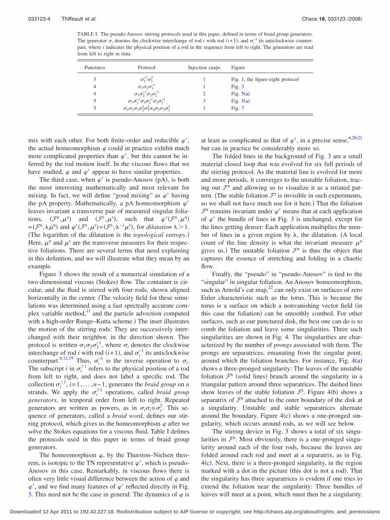
TABLE I. The pseudo-Anosov stirring protocols used in this paper, defined in terms of braid group generators.The generator �i denotes the clockwise interchange of rod i with rod �i+1�, and �i

−1 its anticlockwise counter-part, where i indicates the physical position of a rod in the sequence from left to right. The generators are readfrom left to right in time.

Punctures Protocol Injection cusps Figure

3 �2−2�1

2 1 Fig. 1, the figure-eight protocol4 �1�2�3

−1 1 Fig. 34 �1�2

−1�3�2−1 2 Fig. 5�a�

5 �1�2−1�3�4

−1�3�2−1 3 Fig. 5�a�

5 �1�2�3�23�3

2�4�2�3�23 1 Fig. 7

033123-4 Thiffeault et al. Chaos 18, 033123 �2008�

Downloaded 12 Apr 2011 to 192.43.227.18. Redistribution subject to AIP license or copyright; see http://chaos.aip.org/about/rights_and_permissions

Finally, there is a separatrix connected to the disk’s outerboundary at a singularity, as in Fig. 4�b�, though this is not aseasy to see. From Fig. 4�b� we expect that a boundary sin-gularity will be manifested as a cusp in Fu, a consequence ofthe separatrix emanating from the boundary, and leading toinjection of material into the mixing region �Fig. 3�.

In the pA case, almost every aspect of the Thurston–Nielsen classification theorem can thus be identified directlyin Fig. 3. Rods and the outer boundary possess singularities,and often other �interior� singularities arise in the flow itself,such as the three-pronged singularity indicated by a dot inFig. 3. We will refer to singularities not associated with rodsor the outer boundary as interior singularities. Our referenceprotocol of Fig. 3 demonstrates that the unstable foliation Fu

and its singularities embody many important features of theunderlying flow. We shall thus take the unstable foliation asthe central focus of our study.

III. SINGULARITIES OF THE FOLIATION

An unstable foliation must satisfy three rules if it is tosupport a stirring protocol corresponding to a pseudo-Anosov homeomorphism:23

�1� Every stirring rod �or ghost rod, such as the islands inthe figure-eight protocol� must be enclosed in a one-pronged singularity �Fig. 4�c��. This is a physical re-quirement: One-pronged singularities are the mathemati-cal consequence of physical stirring, since the unstablefoliation wraps around the rod. A rod enclosed in ahigher-pronged singularity makes the rod irrelevant tostirring, since the singularity would exist regardless ofthe rod. Hence, we disregard this possibility.

�2� The outer boundary of the disk contains at least oneseparatrix of Fu, as in Fig. 4�b�. The number of separa-trices on the outer boundary corresponds to the numberof injection cusps into the mixing region.

�3� The smallest number of prongs an interior singularitycan have is 3. This is because two-pronged singularitiesare just regular points �they are not “true” singularitiesof the foliation�, and pseudo-Anosovs do not have one-pronged singularities away from punctures and bound-ary components.

We will use these three rules to limit the number ofallowable singularity data of the unstable foliation Fu. Thesingularity data of a foliation F is the sequence�Nsep ,N3 ,N4 , . . . �, where Nsep is the number of separatriceson the outer boundary, and Np is the number of interiorp-pronged singularities for each p�3. To enumerate the pos-sible distinct singularity data of the unstable foliation for nrods, we use a standard index formula, which relates thenature of the singularities to a topological invariant, the Eu-ler characteristic of the disk; i.e., disk=1.24 This index for-mula says that

n − Nsep − �p�3

�p − 2�Np = 2disk = 2. �1�

Formula �1� is a well-known extension to foliations of theclassical Euler–Poincaré–Hopf formula for vector fields25,26

�see, for example, p. 1352 of Ref. 27�. It is important to notethat the only positive contribution to the left hand side of Eq.�1� is the term n, the number of rods. Hence if there is a largenumber of rods, there must either be a large number of sin-gularities and boundary separatrices, or a small number ofsingularities some of which have many prongs.

In order for Eq. �1� to be satisfied, the boundary separa-trices and interior singularities must contribute �2−n� to theleft hand side. For n=3, the only possibility is to have asingle separatrix on the boundary. There are, therefore,unique singularity data for three stirring rods in a disk, cor-responding to the kidney-shaped region in Fig. 1: The sepa-ratrix on the boundary corresponds to a single injection cuspinto the mixing region.

For n=4, the boundary separatrices and interior singu-larities must contribute −2 to the left hand side of Eq. �1�,which means that there must either be two separatrices on theboundary, or one separatrix on the boundary and an interiorthree-pronged singularity. These two cases correspond to theunstable foliations of the second and third protocols in TableI, as depicted in Figs. 5�a� and 3.

As we add more rods, there are more possibilities for thesingularity data. For example, Fig. 5�b� shows a protocol forfive rods �n=5� with three boundary separatrices �Nsep=3�,corresponding to three injection cusps, and no interior singu-larities.

The maximum number of interior singularities occurswhen there is a single boundary separatrix. The rods and thisseparatrix then contribute n−1 to the left hand side of Eq.�1�, and so Eq. �1� can be satisfied if there are n−3 interiorthree-pronged singularities. That is, the maximum possible

(a)

(b)

FIG. 5. �Color online� Numerical simulations of �a� the stirring protocol�1�2

−1�3�2−1 for four rods, with two injection cusps, and �b� the stirring

protocol �1�2−1�3�4

−1�3�2−1 for five rods, with three injection cusps.

033123-5 Topology of chaotic mixing patterns Chaos 18, 033123 �2008�

Downloaded 12 Apr 2011 to 192.43.227.18. Redistribution subject to AIP license or copyright; see http://chaos.aip.org/about/rights_and_permissions

number of interior singularities occurs for N3=n−3. On theother hand, in order to have no interior singularities, it isnecessary to have n−2 boundary separatrices. This corre-sponds to the maximum possible number of injection cuspsinto the stirring region.

Table II provides a complete summary of the allowablesingularity data for the first few values of n. The number ofpossible distinct singularity data for a foliation increasessharply with the number of rods n, as is evident in Fig. 6�solid line�. A convenient expression for the number of sin-gularity data is

# of singularity data = �k=0

n−3

p�k� , �2�

where p�k� is a partition function.28 The partition functioncounts how many distinct ways positive integers can sum tok, with p�0� defined as 1,

p�k� = # of elements in the set �S � Z+ : �i�S

i = k . �3�

The partition function has no simple exact closed form. Tofind the asymptotic form of Eq. �2� for large n, we can usethe Hardy-Ramanujan asymptotic form for p�k�, and replacethe sum by an integral, to get

# of singularity data 1

2�2�n − 3�exp��2�n − 3�/3�,

n � 1. �4�

The dashed line in Fig. 6 shows that the aysmptotic formcaptures the correct order of magnitude for large n.

IV. HYPERBOLIC INJECTION CUSPS

Injection cusps are not always as plainly visible as in thecases presented thus far. However, as we will see in thissection, their presence can still be inferred by examining thetopological properties of the rod motion, including if neces-sary the motion of ghost rods. This section also helps toclarify the type of topological information that can begleaned from the motion of rods:7,15,29

• If the motion of the rods themselves forms a pseudo-Anosov braid, then the rod motion yields interesting topo-logical information even with no knowledge of ghost rods.This is the case with all the protocols in the paper thus far�except the figure-eight, which involves two obvious ghostrods�. The topological information is then “robust,” in thesense that it does not depend on the specific hydrodynam-ics of the fluid.

• If the motion of the rods does not imply a pseudo-Anosov,such as when there is only one or two rods,6 and chaoticbehavior is observed regardless, then ghost rods must beincluded. This means either looking for regular islands �asin the example in this section� or for unstable periodicorbits. However, the presence and location of such periodicstructures depend on the specific hydrodynamic model�here, Stokes flow for a viscous fluid�.

The protocol discussed in the present section is of thelatter type. Figure 7�a� shows a material line advected by aone-rod stirring device, where the rod follows an epitro-choidal path. The path of the rod is shown as a solid line inFig. 7�b�, superimposed on a Poincaré section. We make twoobservations about Fig. 7: �i� The Poincaré section reveals amixed phase space, consisting of a large chaotic region andseveral smaller regular regions, including a regular regionthat completely encloses the wall. �ii� The injection cuspsinto the mixing region are not readily apparent, though smallcusps are visible.

The presence of the chaotic region can be understood byexamining the motion of the physical rod and of the regularislands visible in Fig. 7�b�. These regular islands are theghost rods that we use to explain the topological propertiesof the homeomorphism � induced by the rod motion, as ana-lyzed in Ref. 7. The braid formed by the rod and the ghostrods is �1�2�3�2

3�32�4�2�3�2

3, which can be shown �withsoftware such as Ref. 30� to correspond to a pseudo-Anosov

TABLE II. The allowable singularity data �Nsep ,N3 ,N4 , . . . � for n rods. Eachrod has a one-pronged singularity, and formula �1� must be satisfied. Nsep

gives the number of separatrices on the outer boundary, and Np gives thenumber of p-pronged interior singularities.

n Nsep N3 N4 N5

3 14 2 04 1 15 3 0 05 2 1 05 1 2 05 1 0 16 4 0 0 06 3 1 0 06 2 2 0 06 2 0 1 06 1 3 0 06 1 1 1 06 1 0 0 1

0 10 20 30 40 5010

0

102

104

106

# of punctures, n

#ofsi

ngula

rity

data

FIG. 6. �Color online� The number of distinct singularity data increasesrapidly with the number of punctures �or rods�. The solid line is exact and isobtained by summing partition functions as in Eq. �2�; the dashed line is theasymptotic form �4�.

033123-6 Thiffeault et al. Chaos 18, 033123 �2008�

Downloaded 12 Apr 2011 to 192.43.227.18. Redistribution subject to AIP license or copyright; see http://chaos.aip.org/about/rights_and_permissions

isotopy class with a single separatrix on the boundary, aswell as two interior three-pronged singularities. Thesingularity data is thus �Nsep=1 ,N3=2� for n=5 rods—seeTable II.

This brings us to our second observation: Where is theinjection cusp associated with the boundary separatrix, aspredicted by the braid? The injection cusp is there, though itis much less evident than those in Figs. 1, 3, and 5. This isbecause here the separatrix is associated with a hyperbolicfixed point, as opposed to parabolic in the previous cases. Aninjection cusp near a parabolic point on the boundary hasvery “slow” dynamics near the separatrix, meaning that fluidapproaches the separatrix very slowly.1 This makes the sepa-ratrices clearly visible as unmixed “tongues” in Figs. 1, 3,and 5.

In contrast, the injection into the mixing region is gov-erned here by a period-3 hyperbolic orbit near the boundaryof the central mixing region. The orbit—consisting of theiterates i0, i1, and i2—is shown in Fig. 7�a�. Notice that theorbit itself does not enter the central mixing region, just as inthe cases previously considered the parabolic fixed points atthe wall remain there. However, a portion of the unstablemanifold of each iterate is shown in Fig. 8: Notice how theunstable manifold of iterate i2 enters the heart of the mixingregion, following the rod. This unstable manifold is theboundary separatrix predicted by the braid. Thus, the way inwhich fluid enters the mixing region is by coming near i2 andthen being dragged along its unstable manifold. The iterates

i0 and i1 play no role as far as injection into the mixingregion is concerned. With hindsight, we can see the unstablemanifold of i2 in the wake of the rod in Fig. 7�a�. Becausethe dynamics in their vicinity is exponential rather than al-gebraic, hyperbolic injection cusps can dramatically speedup the rate of mixing31 in the central region. The price to payis an unmixed region around the wall of the device.

V. DISCUSSION

A stirring device consisting of moving rods undergoingperiodic motion induces a mapping of the fluid domain toitself. This mapping can be regarded as a homeomorphism ofa punctured surface to itself, where the punctures mimic themoving rods. Having the rods undergo a complex braidingmotion guarantees a minimal amount of topological entropy,where by “complex” we mean that the isotopy class associ-ated with the braid is pseudo-Anosov. The topological en-tropy is itself a lower bound on the rate of stretching ofmaterial lines, a quantity which is important for chaoticmixing.

Topological considerations also predict the nature of theinjection of unmixed material into the central mixing region.The number of boundary separatrices in the pseudo-Anosovhomeomorphism’s unstable foliation determines the numberof such injection cusps. The number and position of injectioncusps is particularly important for open flows, such as flowsin channels, since there the nature of injection has a profoundimpact on the shape of the downstream mixing pattern�Fig. 2�.

Topological index formulas allow us to predict the pos-sible types of unstable foliations that can occur for a fixednumber of rods. We did not provide a way of deriving thetopological type of the unstable foliation for a given rodstirring protocol. This can be done, for instance, by using animplementation30 of the Bestvina–Handel algorithm.32 Usingthe enumeration presented here, a mixing device can be de-signed with a specific number of injection cusps into themixing region, by allowing for enough rods and choosing theappropriate stirring protocol.

More generally, instead of physical rods we can considerperiodic orbits associated with a stirring protocol. We callsuch periodic orbits “ghost rods” when they play a similar

i2

i0

i1

(a)

(b)

FIG. 7. �Color online� �a� Numerical simulation of a single rod tracing outan epitrochoidal path �solid line in �b�� stretching a material line for sevenperiods. The period-3 orbit discussed in the text is shown superimposed,with iterates i0, i1, and i2. �b� A Poincaré section �stroboscopic map� of somerepresentative trajectories shows that the phase space consists of a largechaotic region and several regions of regular behavior.

i2

i0

i1

FIG. 8. �Color online� Portions of the unstable manifold of each iterate ofthe period-3 hyperbolic orbit near the boundary of the mixing region. Theunstable manifold of iterate i2 enters the mixing region and corresponds tothe location of the injection cusp.

033123-7 Topology of chaotic mixing patterns Chaos 18, 033123 �2008�

Downloaded 12 Apr 2011 to 192.43.227.18. Redistribution subject to AIP license or copyright; see http://chaos.aip.org/about/rights_and_permissions

role to physical rods �that is, material lines fold around themas if they were rods�.7,12,15,29,33 The topological descriptionpresented here applies to the unstable foliation associatedwith periodic orbits.

In future work, we will consider not just the number ofinjection cusps, but their relative position as well. Indeed,observe that in Fig. 5�b� the position of the injection cuspsalternates sides relative to the line of rods. This is thought tobe a general feature of pseudo-Anosov stirring protocols, butthe proof of this requires careful consideration of whether ornot given foliations are dynamically allowable, in the sensethat they can be realized as the unstable foliation of apseudo-Anosov homeomorphism.

ACKNOWLEDGMENTS

Several of the authors were first introduced to theseideas by Philip Boyland, to whom we are extremely gratefulfor many stimulating discussions.

1E. Gouillart, N. Kuncio, O. Dauchot, B. Dubrulle, S. Roux, and J.-L.Thiffeault, Phys. Rev. Lett. 99, 114501 �2007�.

2H. Aref, J. Fluid Mech. 143, 1 �1984�.3H. Aref, Phys. Fluids 14, 1315 �2002�.4A. Fathi, F. Laundenbach, and V. Poénaru, Asterisque 66–67, 1 �1979�.5W. P. Thurston, Bull., New Ser., Am. Math. Soc. 19, 417 �1988�.6P. L. Boyland, H. Aref, and M. A. Stremler, J. Fluid Mech. 403, 277�2000�.

7E. Gouillart, M. D. Finn, and J.-L. Thiffeault, Phys. Rev. E 73, 036311�2006�.

8P. L. Boyland, M. A. Stremler, and H. Aref, Physica D 175, 69 �2003�.9A. Vikhansky, Phys. Fluids 15, 1830 �2003�.

10M. D. Finn, S. M. Cox, and H. M. Byrne, J. Fluid Mech. 493, 345 �2003�.11M. D. Finn, S. M. Cox, and H. M. Byrne, Phys. Fluids 15, L77 �2003�.12J.-L. Thiffeault, Phys. Rev. Lett. 94, 084502 �2005�.

13J.-L. Thiffeault and M. D. Finn, Philos. Trans. R. Soc. London, Ser. A364, 3251 �2006�.

14T. Kobayashi and S. Umeda, in Proceedings of the International Workshopon Knot Theory for Scientific Objects, Osaka, Japan �Osaka MunicipalUniversities Press, Osaka, 2007�, p. 97.

15B. J. Binder and S. M. Cox, Fluid Dyn. Res. 49, 34 �2008�.16M. D. Finn, J.-L. Thiffeault, and E. Gouillart, Physica D 221, 92 �2006�.17M. D. Finn and J.-L. Thiffeault, SIAM J. Appl. Dyn. Syst. 6, 79 �2007�.18S. C. Jana, G. Metcalfe, and J. M. Ottino, J. Fluid Mech. 269, 199 �1994�.19J. S. Birman, Braids, Links, and Mapping Class Groups, in Annals of

Mathematics Studies �Princeton University Press, Princeton, 1975�.20M. Handel, Ergod. Theory Dyn. Syst. 8, 373 �1985�.21P. L. Boyland, Contemp. Math. 246, 17 �1999�.22V. I. Arnold and A. Avez, Ergodic Problems of Classical Mechanics �W.

A. Benjamin, New York, 1968�.23R. C. Penner and J. L. Harer, Combinatorics of Train Tracks, in Annals of

Mathematics Studies Vol. 125 �Princeton University Press, Princeton,1991�.

24More generally, the Euler characteristic of a surface of genus g with bboundaries is 2−2g−b, where the genus is the number of “handles” at-tached to a sphere. In particular, sphere=2, disk=2−1=1, and torus=2−2·1=0.

25J. W. Milnor, Topology from the Differentiable Viewpoint, revised edition�Princeton University Press, Princeton, 1997�.

26W. P. Thurston, Three-dimensional Geometry and Topology, edited by S.Levy �Princeton University Press, Princeton, 1997�, Vol. 1.

27G. Band and P. L. Boyland, Algebraic Geom. Topol. 7, 1345 �2007�.28G. E. Andrews, The Theory of Partitions �Addison-Wesley, Reading,

1976�.29M. A. Stremler and J. Chen, Phys. Fluids 19, 103602 �2007�.30T. Hall, “Train: A C�� program for computing train tracks of sur-

face homeomorphisms,” http://www.liv.ac.uk/maths/PURE/MIN_SET/CONTENT/members/T_Hall.html.

31E. Gouillart, Ph.D. thesis, Université Pierre et Marie Curie Paris 6, 2007,http://tel.archives-ouvertes.fr/tel-00204109/en.

32M. Bestvina and M. Handel, Topology 34, 109 �1995�.33J.-L. Thiffeault, E. Gouillart, and M. D. Finn, “The size of ghost rods,”

arXiv:nlin/0507076.

033123-8 Thiffeault et al. Chaos 18, 033123 �2008�

Downloaded 12 Apr 2011 to 192.43.227.18. Redistribution subject to AIP license or copyright; see http://chaos.aip.org/about/rights_and_permissions