Well Logging Tools and TechniquesMagnetic Resonance Logs

INTRODUCTIONIn this section, we’ll review NMR concepts, compare NMR tools to other logging tools, discuss current tool types, and briefly look at examples of NMR logs.

ACKNOWLEDGEMENTIHRDC wishes to express their gratitude to Numar, a Halliburton Company, for graciously contributing resources, technical input, and graphics pertaining to NMR theory, as well as information on their MRIL logging tool and associated services. Further details on this subject can be found in NMR Logging Principles and Applications, (1999) by Coates, Xiao, and Prammer. (See the References section for a complete listing.) Additional information on Halliburton/Numar MRIL services can be found on-line. Look under the Logging and Perforating section at www.halliburton.com .

IHRDC also thanks Schlumberger for graphics and information pertaining to their CMR tool. Additional information on the Schlumberger CMR tool can be found at www.connect.slb.com .

BACKGROUNDSince its discovery in 1946, nuclear magnetic resonance (NMR) has developed into a valuable tool for physics, chemistry, biology, and medicine. The potential for applying this technology to formation evaluation was identified during the 1950’s. Early logging tools had very limited application and the majority of the work was related to core analysis. With the invention of NMR logging tools that use permanent magnets and pulsed radio frequencies, sophisticated laboratory techniques were developed to enable in situ determination of formation properties. This capability opens a new era in formation evaluation and core analysis, just as the introduction of NMR has revolutionized the other scientific areas to which it has been applied.

CONCEPTTo understand the concept and applications for NMR in formation evaluation, it may be helpful to review and compare the use of magnetic resonance imaging (MRI) in the medical field.

MRI is one of the most valuable clinical diagnostic tools in health care today. With a patient placed in the whole-body compartment of an MRI system, magnetic resonance signals from hydrogen nuclei at specific locations in the body can be detected and used to construct an image of the interior structure of the body. These images may reveal physical abnormalities and thereby aid in the diagnosis of injury and disease.

The MRI of the human head in Figure   1 (Medical MRI presentation) demonstrates two important

MRI characteristics.

Figure 1

First, the signals used to create each image come from a well-defined location, typically a thin slice or cross section of the target. Because of the physical principles underlying NMR technology, each image is sharp, containing only information from the imaged cross section, with material in front or behind being essentially invisible.

Second, only fluids (seen in blood vessels, body cavities, and soft tissues) are visible, while solids (such as bone) produce a signal that typically decays too fast to be recorded. By taking advantage of these two characteristics, physicians have been able to make valuable diagnostic use of MRI -without needing to understand complex NMR principles.

These same NMR principles, instead of being used to diagnose anomalies in the human body, can be used to analyze the fluids held in the pore spaces of reservoir rocks. And, just as physicians do not need to be NMR experts to use MRI technology for effective medical diagnosis, neither do geologists, geophysicists, petroleum engineers, nor reservoir engineers need to be NMR experts to use MRI logging technology for reliable formation evaluation.

In an NMR Logging tool, a permanent magnet produces a magnetic field that excites formation materials. An antenna transmits into the formation precisely timed bursts of radio-frequency energy in the form of an oscillating magnetic field. Between these pulses, the antenna is used to listen for the decaying “echo” signal from those hydrogen protons that are in resonance with the field from the permanent magnet. Since this magnetic resonant frequency depends on the local strength of the magnetic field, the measurement zone of the tool is a function of the magnetic field generated, and the radio frequency used. These tool operations will be discussed in more detail in the sections to follow.

COMPARING NMR TOOLS TO OTHER LOGGING TOOLSBecause only fluids are visible to NMR, the porosity measured by an NMR tool contains no contribution from the matrix materials, and therefore does not need to be calibrated to formation

lithology. This response characteristic makes NMR tools fundamentally different from conventional logging tools.

The conventional neutron, bulk-density, and acoustic-travel-time porosity-logging tools are influenced by components of the reservoir rock. Because reservoir rocks typically have more rock framework than fluid-filled space, these conventional tools tend to be much more sensitive to the matrix materials than to the pore fluids.

Conventional resistivity-logging tools, while being extremely sensitive to the fluid-filled space and traditionally used to estimate the amount of water present in reservoir rocks, cannot be regarded as true fluid-logging devices. These tools are strongly influenced by the presence of conductive minerals and, for the responses of these tools to be properly interpreted, a detailed knowledge of the properties of both the formation and the water in the pore space is required.

Unique Formation MeasurementsNMR tools can provide three types of information, each of which make these tools unique among logging devices:

information about the quantities of the fluids in the rock,

information about the properties of these fluids, and

information about the sizes of the pores that contain these fluids.

Current Tool TypesMagnetic Resonance Imaging Logging (MRIL), introduced by NUMAR in 1991, takes the medical MRI or laboratory NMR equipment and turns it inside-out. So, rather than placing the subject to be analyzed at the center of the instrument, the instrument itself is placed, in a wellbore, at the center of the formation to be analyzed. This tool is used by Numar, a Halliburton company and by Baker Atlas, a Baker Hughes company.

The Schlumberger tool, the Combinable Magnetic Resonance tool (CMR), follows on from earlier Schlumberger NMR tools that date back to the 1970s. The CMR is a pad-type tool, which uses a directional antenna sandwiched between a pair of bar magnets to focus the CMR measurement on a 6-in. [15-cm] long zone inside the formation—the same rock volume scanned by other essential logging tools.

LOG EXAMPLESThis first example, shown in Figure   2 (Example of CMR porosity log) demonstrates how NMR

porosity (in this case from a Schlumberger CMR tool) is independent of lithology,

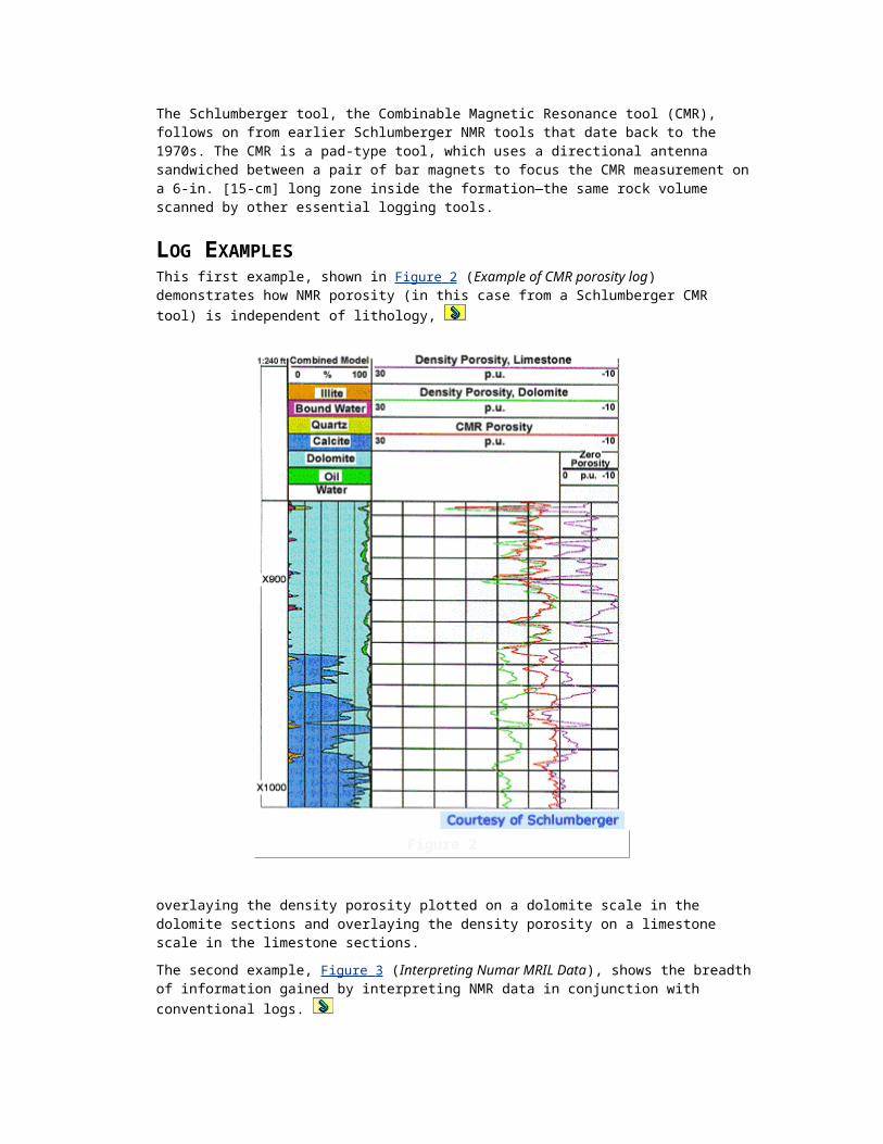
Figure 2

overlaying the density porosity plotted on a dolomite scale in the dolomite sections and overlaying the density porosity on a limestone scale in the limestone sections.

The second example, Figure   3 (Interpreting Numar MRIL Data), shows the breadth of information

gained by interpreting NMR data in conjunction with conventional logs.

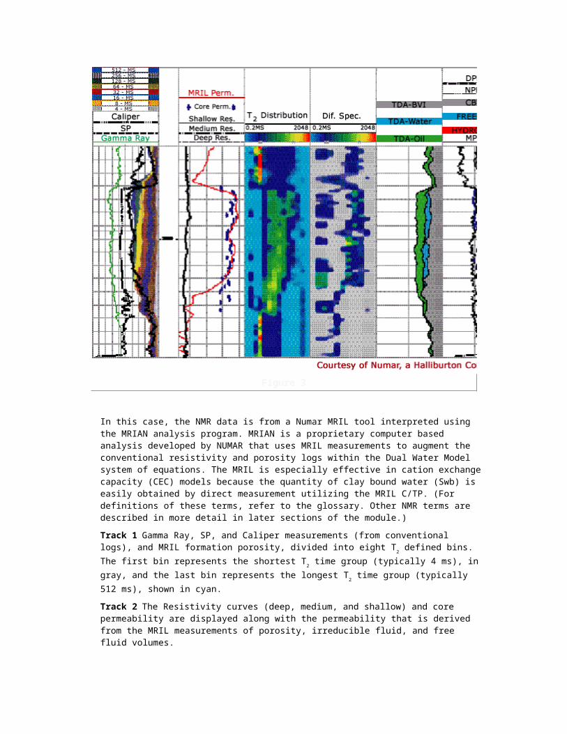
Figure 3

In this case, the NMR data is from a Numar MRIL tool interpreted using the MRIAN analysis program. MRIAN is a proprietary computer based analysis developed by NUMAR that uses MRIL measurements to augment the conventional resistivity and porosity logs within the Dual Water Model system of equations. The MRIL is especially effective in cation exchange capacity (CEC) models because the quantity of clay bound water (Swb) is easily obtained by direct measurement utilizing the MRIL C/TP. (For definitions of these terms, refer to the glossary. Other NMR terms are described in more detail in later sections of the module.)

Track 1 Gamma Ray, SP, and Caliper measurements (from conventional logs), and MRIL formation porosity, divided into eight T

2 defined bins. The first bin represents the shortest T

2 time

group (typically 4 ms), in gray, and the last bin represents the longest T2 time group (typically 512

ms), shown in cyan.

Track 2 The Resistivity curves (deep, medium, and shallow) and core permeability are displayed along with the permeability that is derived from the MRIL measurements of porosity, irreducible fluid, and free fluid volumes.

Track 3 The T2 distribution, also presented in Track 1 in a bin format, is illustrated in this track in

a variable density format. T2 time is logarithmically spaced across the track from 0.2 ms on the left

edge to 2048 ms on the right edge of the track. The amount of porosity that is represented by each T

2 value (partial porosity) is illustrated by color; blue represents zero partial porosity and red

represents the highest partial porosity. Since the bound (clay or capillary) fluids are represented by the short T

2 times, they will be seen on the left portion of the track, while increasing volumes

are represented by the colors shown. The free fluids are represented by longer T2 times and are

seen in the middle and the right portions of the track.

Track 4 The results of the Differential Spectrum Method (DSM) are displayed in this VDL format. The difference between two T

2 spectra, each taken at a different wait time (Tw), yields the

hydrocarbon signal. Relative position indicates hydrocarbon type, and color is proportional to volume.

Track 5 Time Domain Analysis (TDA) computes an MRIL only result yielding all the major fluid volumes. In addition to these MRIL volumes, fluid typing indicates, independently, gas (red), oil (green), and water (blue), and where fluid contacts may exist.

Track 6 This track contains a playback of the conventional neutron and density porosity curves along with the MRIL. These porosities are further divided into four volumes: the irreducible fluid volume (light gray), the hydrocarbon filled portion (red), moveable water (blue), and clay bound water (dark gray). The Dual Water Model is used to compute both the total and effective volumes of water, using only conventional log data, then the effective water volume is compared with the irreducible volume from the MRIL. When the computed effective volume of water is greater than the MRIL irreducible volume of water, water production is inferred.

 

 PRINCIPLES OF OPERATIONThis section provides an overview of NMR Fundamentals, Logging Basics, Relaxation mechanisms, and Pore Fluid Effects

NMR FUNDAMENTALS Nuclear magnetic resonance refers to the way in which nuclei respond to a magnetic field. Many nuclei have a magnetic moment -they behave like spinning bar magnets. These spinning magnets can interact with externally applied magnetic fields, producing measurable signals. For most elements the detected signals are small. However, hydrogen, which makes up a significant component of both water and hydrocarbons in the pore spaces of rock, has a relatively large magnetic moment.

NMR LOGGING BASICSBefore a formation is logged by an NMR logging tool, the protons in the formation fluids are randomly oriented. When the tool passes through the formation, the tool generates magnetic fields that activate those protons.

First, the tool's permanent magnetic field aligns, or polarizes, the spin axes of the protons in a particular direction. This process, called polarization, increases exponentially in time with a time constant, designated as T1.

Next, the tool's oscillating field is applied to tip these protons away from their new equilibrium position in the same way a child’s spinning top precesses in the Earth’s gravitational field. Precession occurs as a body rotating about one axis slowly rotates around a second axis. In the NMR case, this second axis is the static magnetic field. This is shown in Figure   1 (Spin

precession).

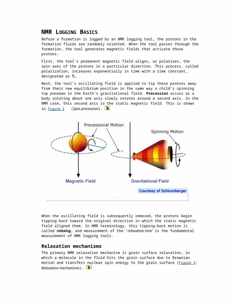
Figure 1

When the oscillating field is subsequently removed, the protons begin tipping back toward the original direction in which the static magnetic field aligned them. In NMR terminology, this tipping-back motion is called relaxing, and measurement of the ‘relaxation time’ is the fundamental measurement of NMR logging tools.

Relaxation mechanismsThe primary NMR relaxation mechanism is grain surface relaxation, in which a molecule in the fluid hits the grain surface due to Brownian motion and transfers nuclear spin energy to the grain surface (Figure   2 : Relaxation mechanisms).

Figure  2

The effectiveness of the process depends on the surface: sandstones are about 3 times as efficient at relaxing pore water as carbonates.

Bulk fluid relaxation occurs in the absence of pore surface interaction. It is significant in large pore spaces such as vuggy carbonates, and also when hydrocarbons are present. Bulk fluid relaxation is seen in hydrocarbons because the non-wetting phase does not contact the pore surface, so it cannot be relaxed by the surface relaxation method.

Specified pulse sequences are used to generate a series of so-called spin echoes, which are measured by the NMR logging tool and are displayed on logs as spin-echo trains. These spin-echo trains constitute the raw NMR data.

To generate a spin-echo train, the NMR tool measures the amplitude of the spin echoes as a function of time (Figure   3 : Spin-echo train display).

Figure 3

Because the spin echoes are measured over a short time, the NMR tool travels no more than a few inches in the well while recording the spin-echo train. The recorded spin-echo trains can be displayed on a log as a function of depth.

The initial amplitude of the spin-echo train is proportional to the number of hydrogen nuclei associated with the fluids in the pores within the sensitive volume. Thus, this amplitude can be calibrated to provide porosity.

The observed echo train can be linked both to data-acquisition parameters and to properties of the pore fluids located in the measurement volumes. Data acquisition parameters include inter-echo spacing (TE) and polarization time (TW). TE represents the time between the individual echoes in an echo train. TW represents the time between the cessation of measurement of one echo train and the beginning of measurement of the next echo train. Both TE and TW can be adjusted to change the information content of the acquired data.

Pore Fluid EffectsProperties of the pore fluids that affect the echo trains are the:

Hydrogen Index (HI): a measure of the density of hydrogen atoms in the fluid

Longitudinal Relaxation Time (T1): an indication of how fast the tipped protons in the fluids relax longitudinally (relative to the axis of the static magnetic field)

Transverse Relaxation Time (T2): an indication of how fast the tipped protons in the fluids relax transversely (again, relative to the axis of the static magnetic field)

Diffusivity (D): a measure of the extent to which molecules move at random in the fluid.

TOOL DESCRIPTIONThis section describes NMR logging tools developed by Numar and by Schlumberger.

NUMAR’S MRIL TOOLMagnetic Resonance Imaging Logging (MRIL), introduced by NUMAR in 1991, takes the medical MRI or laboratory NMR equipment, and turns it inside-out. Rather than placing the subject to be analyzed at the center of the instrument, the instrument itself is placed in the wellbore, at the center of the formation to be analyzed. MRIL services are provided by Numar, a Halliburton company and by Baker Atlas, a Baker Hughes company.

At the center of the MRIL tool, a permanent magnet produces a magnetic field that excites formation materials. An antenna surrounding this magnet transmits into the formation precisely timed bursts of radio-frequency energy in the form of an oscillating magnetic field. Between these pulses, the antenna is used to listen for the decaying “echo” signal from those hydrogen protons that are in resonance with the field created by the permanent magnet.

Because a linear relationship exists between the proton resonance frequency and the strength of the permanent magnetic field, the frequency of the transmitted and received energy can be tuned to investigate cylindrical regions at different diameters around the MRIL tool. This tuning of the MRI probe to be sensitive to a specific frequency allows MRI instruments to image narrow slices of the rock formation.

Figure   1 (Cylinders of investigation) illustrates the measurement concept behind Numar’s MRIL-

Prime tool, which was introduced in 1998.

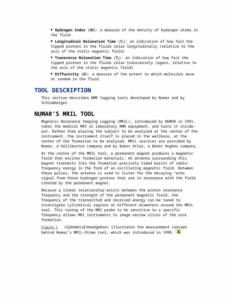
Figure 1

The diameter and thickness of each thin cylindrical region are selected by simply specifying the central frequency and bandwidth to which the MRIL transmitter and receiver are tuned. The diameter of the cylinder is temperature dependent, but typically ranges from approximately 14 to 16 inches.

SCHLUMBERGER’S CMR TOOLThe Schlumberger Combinable Magnetic Resonance tool (designated as the CMR tool) follows on from earlier Schlumberger NMR tools that date back to the 1970s. It uses a directional antenna sandwiched between a pair of bar magnets to focus the CMR measurement on a 6-in. [15-cm] zone inside the formation—the same rock volume scanned by other essential logging measurements. As shown in Figure   2 (CMR tool), it is a compact skid-mounted tool that was

designed to be combinable with many other standard logging tools.

Figure 2

The vertical resolution of the CMR measurement makes it sensitive to rapid porosity variations, as often seen in laminated shale and sand sequences.

The first pulsed-echo NMR logging tools introduced in the early 1990s, were unable to detect the fast components of resonance decay. The shortest T2 was limited to the 3 to 5 msec range, which allowed measurement of capillary-bound water and free fluids together, to derive effective porosity. However, clay-bound water, being more tightly bound, is believed to decay at a much faster rate than was measurable with these tools. The latest improvements in these tools measure decay rates at a much higher speed -by a factor of ten. Now, measuring T2 decay components in the 0.1 to 0.5-msec range is possible. These improvements include electronic upgrades, more efficient data acquisition, and new signal-processing techniques that take advantage of the early-time information. The CMR tool is run in an eccentered configuration.

The sensitive region of the tool is shown in red in Figure   3 (Cross-section of the CMR tool).

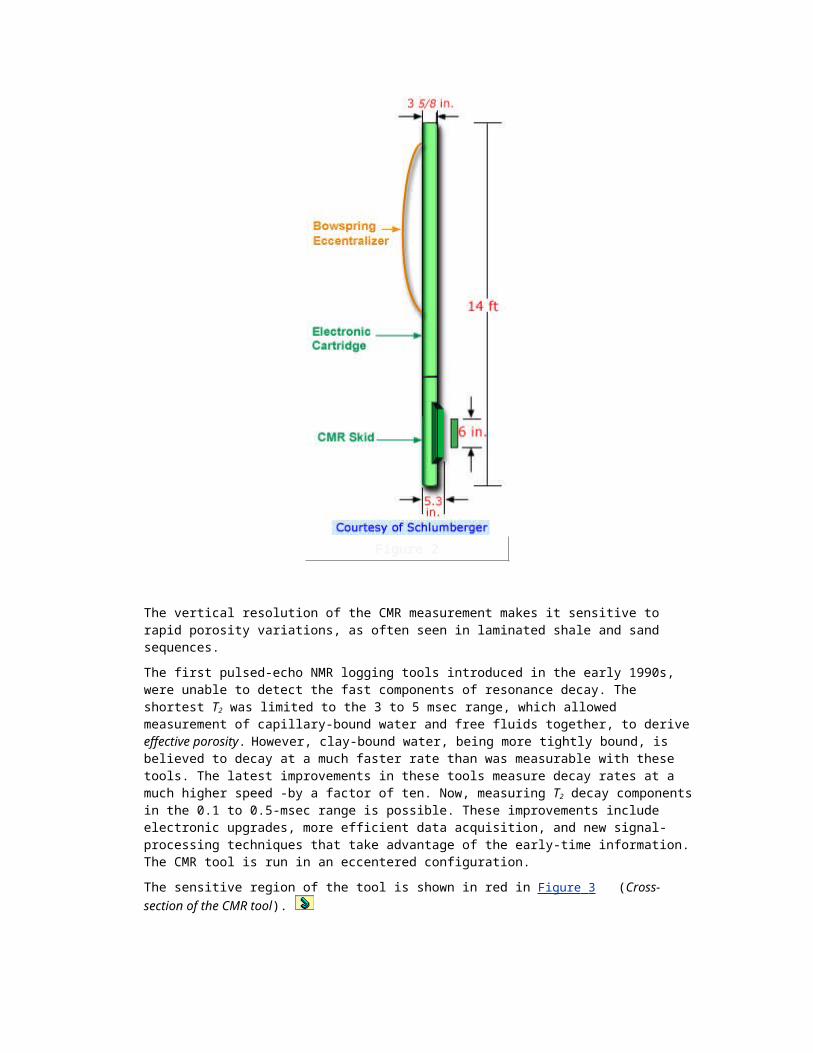
Figure  3

This region is approximately 0.5” x 0.5” by 6” long, and is located about 1.1 inches inside the formation.

 NMR INTERPRETATION

OVERVIEW

 

All NMR measurements made by current tools are summarized by the T2 distribution. The petrophysical applications of this distribution can be summarized as follows:

The area under the distribution curve equals NMR porosity

T2 distribution mimics pore size distribution in water-saturated rocks

Permeability is estimated from logarithmic-mean T2 and NMR porosity

Empirically derived cutoffs separate the T2 distribution into areas equal to free-fluid porosity and irreducible water porosity

Multiple T2 data sets acquired with different acquisition parameters can differentiate between formation fluids

Properly defined, the area under the T2 distribution curve is equal to the initial amplitude of the spin-echo train. Hence, the T2 distribution can be directly calibrated in terms of water-filled

porosity. In essence, a key function of the NMR tool and its associated data-acquisition software is to provide an accurate description of the T2 distribution at every depth in the wellbore.

The basic physics behind NMR interpretation is common to all the data, however, each of the current NMR logging service companies - Baker Atlas, Numar, and Schlumberger have their own proprietary interpretation methods. In addition, there are now several companies that specialize in the interpretation of NMR data, including NuTech and NMR+.

POROSITYThe initial amplitude of the raw decay curve is directly proportional to the number of polarized hydrogen nuclei within the pore fluid.

The raw reported porosity is provided by the ratio of the initial amplitude of the raw decay to the tool response in a water tank (which provides a medium having 100% porosity). This porosity is independent of the lithology of the rock matrix, and can be validated by comparing laboratory NMR measurements on cores with conventional laboratory porosity measurements.

The accuracy of the raw reported porosity depends primarily on three factors:

a sufficiently long TW, to achieve complete polarization of the hydrogen nuclei in the fluids

a sufficiently short TE, to record the decays for fluids associated with clay pores and other pores of similar size

the number of hydrogen nuclei in the fluid being equal to the number in an equivalent volume of water, that is, HI = 1.

Provided the preceding conditions are satisfied, the NMR porosity is the most accurate porosity reading available in the logging industry.

The first and third factors are only important for gas or light hydrocarbons. In these cases, special activations can be run to provide information to correct the porosity. The second factor was a problem in earlier generations of tools, because they could not, in general, see most of the fluids associated with clay minerals.

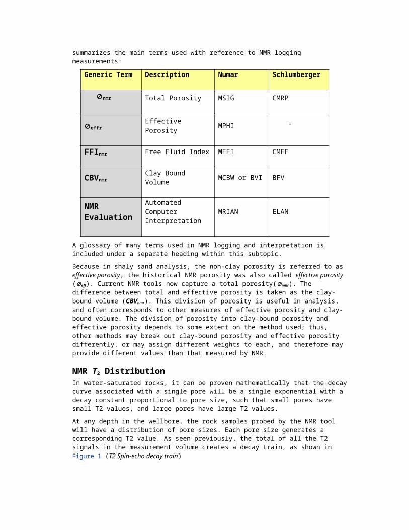
TerminologyThrough this text we have used generic terminology where it makes sense, and used tool-specific terminology as applicable. The following table summarizes the main terms used with reference to NMR logging measurements:

Generic Term 

Description 

Numar 

Schlumberger 

nmr

 

Total Porosity 

MSIG 

CMRP 

effr

 Effective Porosity 

MPHI 

-

 FFInmr

 Free Fluid Index 

MFFI 

CMFF 

CBVnmr

 Clay Bound Volume 

MCBW or BVI 

BFV 

NMR Evaluation 

Automated Computer Interpretation 

MRIAN  

ELAN 

A glossary of many terms used in NMR logging and interpretation is included under a separate heading within this subtopic.

Because in shaly sand analysis, the non-clay porosity is referred to as effective porosity, the historical NMR porosity was also called effective porosity (eff). Current NMR tools now capture a total porosity(nmr). The difference between total and effective porosity is taken as the clay-bound volume (CBVnmr). This division of porosity is useful in analysis, and often corresponds to other measures of effective porosity and clay-bound volume. The division of porosity into clay-bound porosity and effective porosity depends to some extent on the method used; thus, other methods may break out clay-bound porosity and effective porosity differently, or may assign different weights to each, and therefore may provide different values than that measured by NMR.

NMR T2 DistributionIn water-saturated rocks, it can be proven mathematically that the decay curve associated with a single pore will be a single exponential with a decay constant proportional to pore size, such that small pores have small T2 values, and large pores have large T2 values.

At any depth in the wellbore, the rock samples probed by the NMR tool will have a distribution of pore sizes. Each pore size generates a corresponding T2 value. As seen previously, the total of all the T2 signals in the measurement volume creates a decay train, as shown in Figure   1 (T2 Spin-echo decay train)

Figure 1

The amplitude of the spin-echo-train decay can be fit very well by a sum of decaying exponentials, each with a different decay constant. The set of all the decay constants forms the decay spectrum or transverse-relaxation-time (T2) distribution.

Hence, the multi-exponential decay represents the distribution of pore sizes at that depth, with each T2 value corresponding to a different pore size. Figure   2 (T2 distribution) was derived from

the previous figure’s spin-echo train.

Figure 2

The NMR T2 distribution can be displayed in several different ways: Each visualization represents the distribution of the porosity over T2 values and, hence, over the pore sizes.

Figure   3 (MRIL Log) shows a typical NUMAR MRIL presentation.

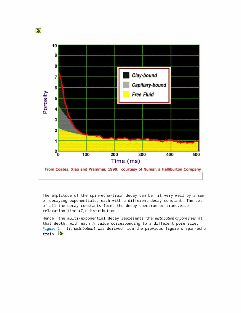
Figure 3

On the MRIL log, T2 distributions are displayed in three ways: A plot of the cumulative amplitudes from the binned T2-distribution is shown in Track 1, a color image of the binned T2-distribution is in Track 3, and a waveform presentation of the same information is in Track 4. The T2-distribution typically displayed for MRIL data corresponds to binned amplitudes for exponential decays at 0.5, 1, 2, 4, 8, 16, 32, 64, 128, 256, 512, and 1024 ms when MSIG is shown, and from 4 ms to 1024 ms when MPHI is shown. The 8-ms bin, for example, corresponds to measurements made between 6 and 12 ms. Because logging data are much noisier than laboratory data, only a comparatively coarse T2-distribution can be created from NMR log data.

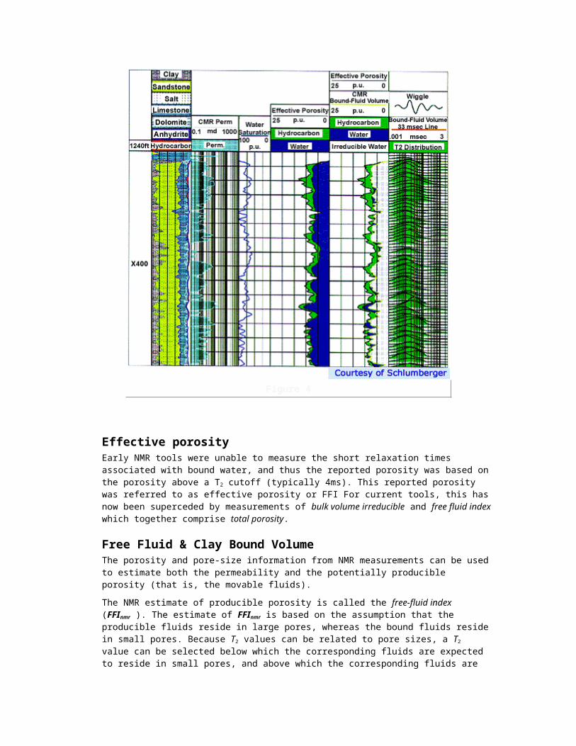
Figure   4 (CMR Log) shows an example of a typical Schlumberger CMR presentation.

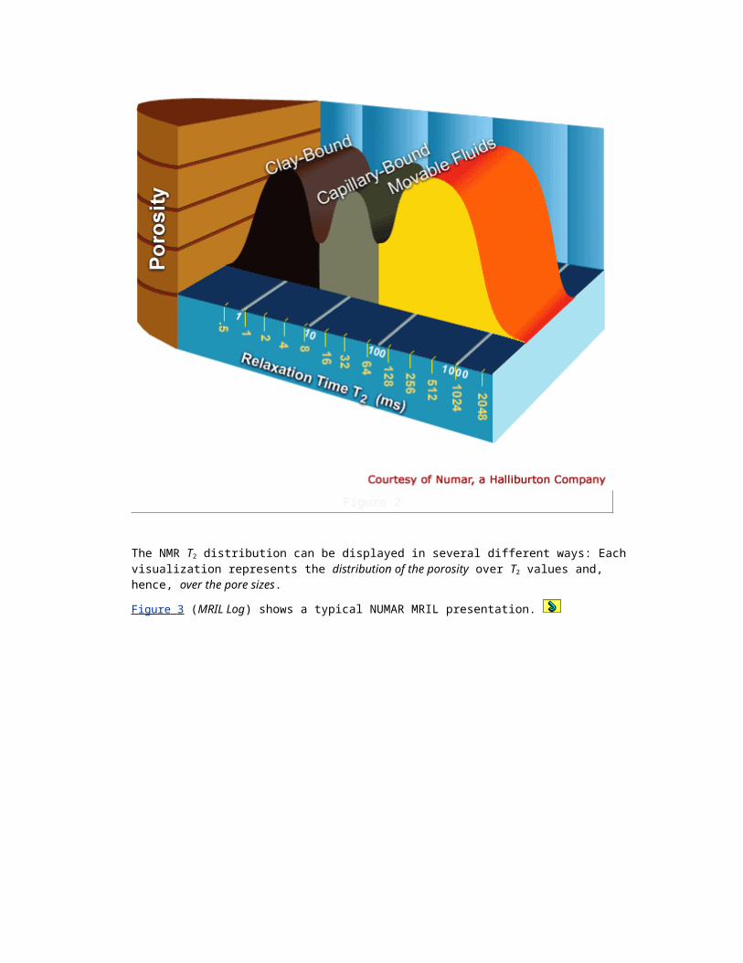
Figure 4

Effective porosityEarly NMR tools were unable to measure the short relaxation times associated with bound water, and thus the reported porosity was based on the porosity above a T2 cutoff (typically 4ms). This reported porosity was referred to as effective porosity or FFI For current tools, this has now been superceded by measurements of bulk volume irreducible and free fluid index which together comprise total porosity.

Free Fluid & Clay Bound Volume The porosity and pore-size information from NMR measurements can be used to estimate both the permeability and the potentially producible porosity (that is, the movable fluids).

The NMR estimate of producible porosity is called the free-fluid index (FFInmr ). The estimate of FFInmr is based on the assumption that the producible fluids reside in large pores, whereas the bound fluids reside in small pores. Because T2 values can be related to pore sizes, a T2 value can be selected below which the corresponding fluids are expected to reside in small pores, and above which the corresponding fluids are expected to reside in larger pores. This T2 value is called the T2 cutoff (T2cutoff).

Through partitioning of the T2 distribution, T2cutoff divides nmr into free-fluid index and bound-fluid porosity, or bulk volume irreducible or clay bound volume (CBVnmr), shown in Figure   5 (T2

distribution).

Figure 5

The T2cutoff can be determined with NMR measurements on water-saturated core samples. Specifically, a comparison is made between the T2 distribution of a sample in a fully water-saturated state, and the same sample in a partially saturated state, the latter typically being attained by centrifuging the core at a specified air-brine capillary pressure.

Although capillary pressure, lithology, and pore characteristics all affect T2cutoff values, common practice establishes local field values for T2cutoff. For example, in the Gulf of Mexico, T2cutoff values of 33 and 92 ms are generally appropriate for sandstones and carbonates, respectively. Generally though, the best values can be obtained by measuring core samples corresponding to the actual interval logged by an NMR tool.

PERMEABILITY NMR relaxation properties of rock samples are dependent on porosity, pore size, pore-fluid properties and mineralogy. The NMR estimate of permeability is based on theoretical models, which show that permeability increases with both increasing porosity and increasing pore size. Two related kinds of permeability models have been developed.

The Free-fluid or Coates model can be applied in formations containing water and/or hydrocarbons.

The average-T2 model Schlumberger-Doll-Research model (SDR) -can be applied to pore systems containing only water.

Measurements on core samples are necessary to refine these models and produce a model customized for local use. Figure   6 (Decay of spin echo train) shows information related to

formation permeability.

Figure 6

Two echo trains were obtained from formations having different permeabilities. Both formations have the same porosity, but also have different pore sizes. This difference leads to shifted T2 distributions, and therefore to different values of the ratio of MFFI to BVI. Also indicated in the Figure are the permeabilities computed from the Coates model

k = [(MPHI / C)2 (MFFI / BVI)]2,

where

k is formation permeability and C is a constant that depends on the formation

Figure   7

Figure 7

(Core permeability crossplot) shows how laboratory core data can be calibrated to determine the constant C in the Coates permeability model. Track 2 of the log in Figure   8 (MRIL permeability

display) demonstrates MRIL permeability derived from a customized Coates model.

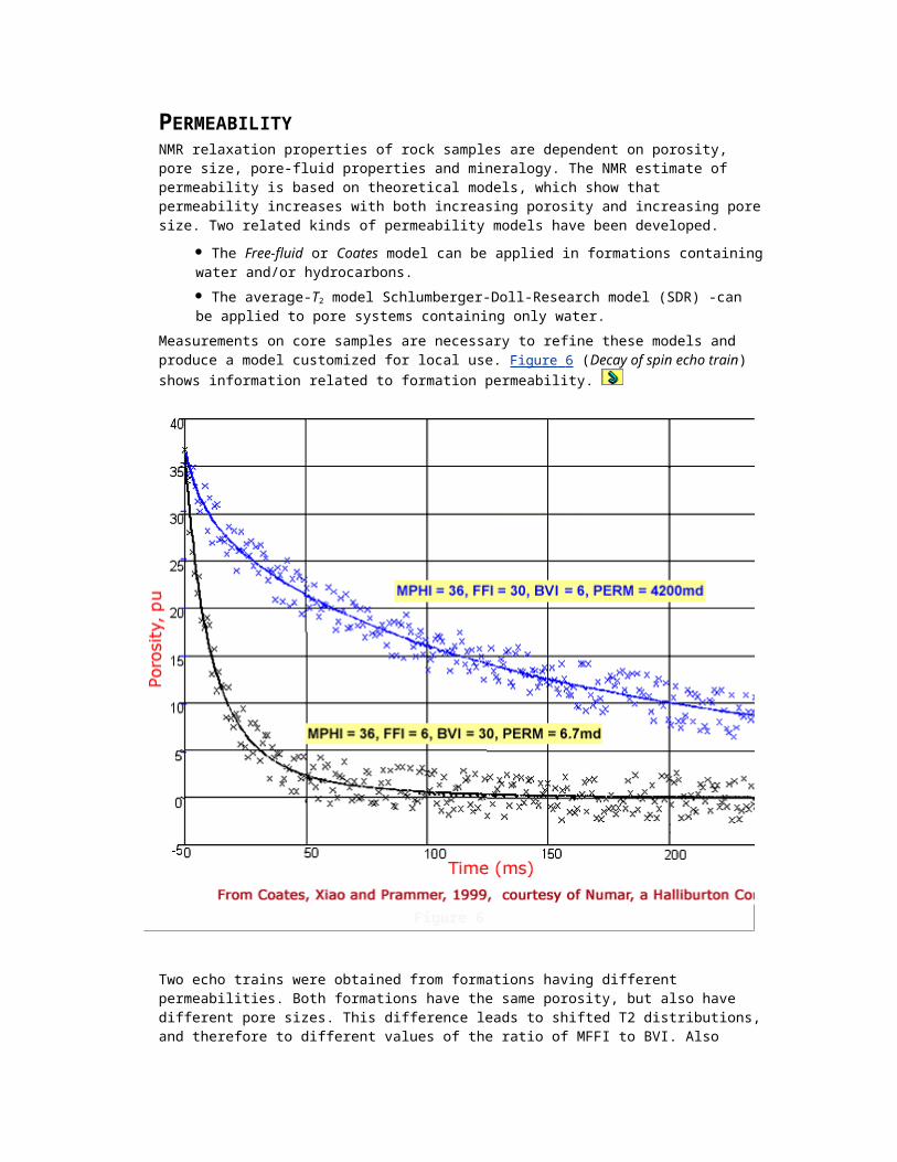
Figure 8

NMR PROPERTIES OF RESERVOIR FLUIDSClay-bound water, capillary-bound water, and movable water occupy different pore sizes and locations. Hydrocarbon fluids differ from brine in their locations in the pore space, usually occupying the larger pores. They also differ from each other and brine in viscosity and diffusivity. NMR logging uses these differences to characterize the fluids in the pore space.

Figure   9 (Typical qualitative values of T1,

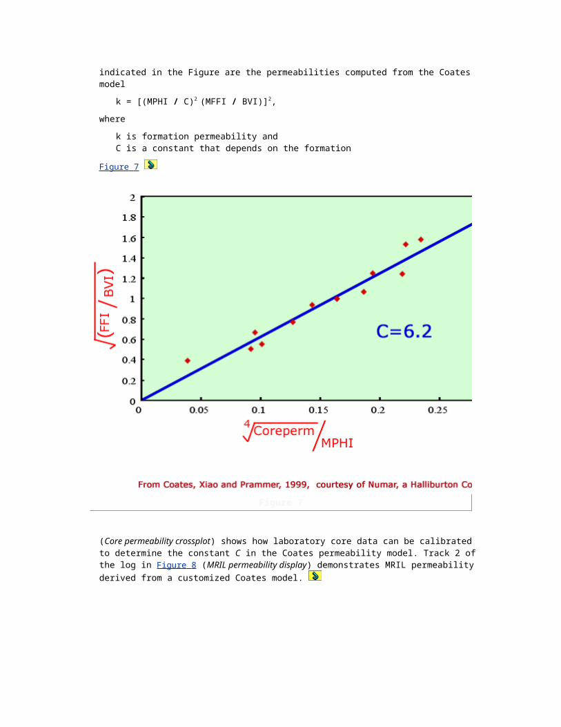
Figure 9

T2, and D for different fluid types and rock pore sizes demonstrate the variability and complexity of the T1 and T2 relaxation measurements.) qualitatively indicates the NMR properties of different fluids found in rock pores. In general, bound fluids have very short T1 and T2 times, along with slow diffusion (small D) that is due to the restriction of molecular movement in small pores. Free water commonly exhibits medium T1, T2, and D values. Hydrocarbons, such as natural gas, light oil, medium-viscosity oil, and heavy oil, also have very different NMR characteristics. Natural gas exhibits very long T1 times but short T2 times and a single-exponential type of relaxation decay. NMR characteristics of oils are quite variable and are largely dependent on oil viscosities. Lighter oils are highly diffusive, have long T1 and T2 times, and often exhibit a single-exponential decay. As viscosity increases and the hydrocarbon mix becomes more complex, diffusion decreases, as do the T1 and T2 times, and events are accompanied by increasingly complex multi-exponential decays. Based on the unique NMR characteristics of the signals from the pore fluids, applications have been developed to identify and, in some cases, quantify the type of hydrocarbon present.

NMR Hydrocarbon Typing Despite variabilities in the NMR properties of fluids, the locations of signals from different types of fluids in the T2 distribution can often be predicted or, if measured data are available, identified. This capability provides important information for NMR data interpretation and makes many applications practical.

Figure   10 (Different T2 distributions)

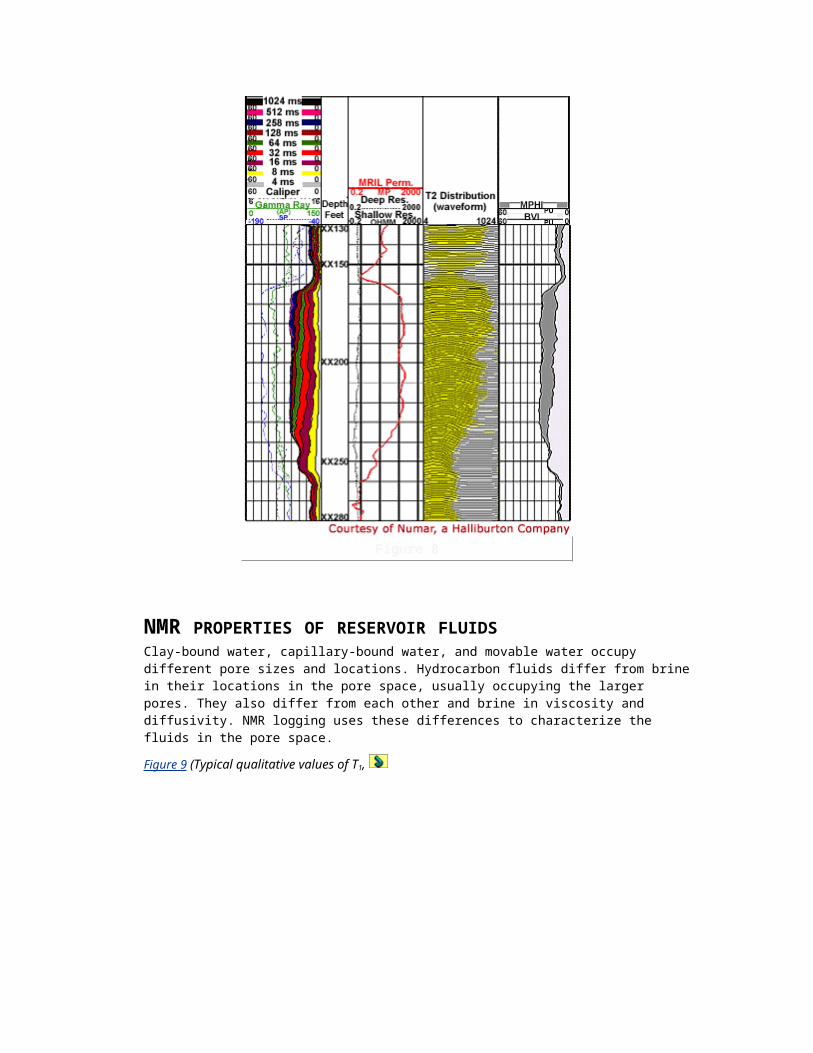
Figure 10

shows two methods for differentiating fluids. In Part a of this figure, different TW values are used with a T1-weighted mechanism to differentiate light hydrocarbons (light oil or gas, or both) from water. In Part b of this figure, different TE values are used with a diffusivity-weighted mechanism in a well-defined gradient magnetic field to differentiate viscous oil from water, or to differentiate gas from liquid.

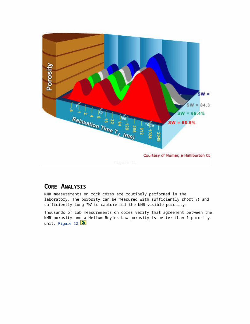
By varying water saturation, it is also possible to produce different T2 distributions, as shown in Figure   11 (Water saturation effects on T2).

Figure 11

CORE ANALYSISNMR measurements on rock cores are routinely performed in the laboratory. The porosity can be measured with sufficiently short TE and sufficiently long TW to capture all the NMR-visible porosity.

Thousands of lab measurements on cores verify that agreement between the NMR porosity and a Helium Boyles Law porosity is better than 1 porosity unit. Figure   12

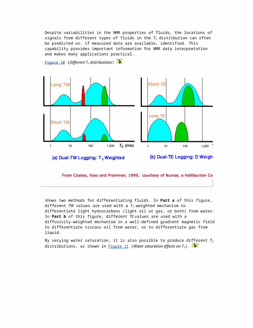
Figure 12

(NMR-core porosity plot) illustrates such an agreement.

As exemplified in this figure, with a set of clean sandstones, good agreement is typically observed between porosity derived from laboratory NMR measurements and porosity derived from conventional core analysis. NMR-porosity values typically fall within ±1 p.u. of the measured core-porosity values. The Figure shows NMR laboratory data measured at two different TE values, namely, 0.5 and 1.2 ms. A comparison of core data to NMR data provides an indication as to whether micro-porosity is present. (Fluid in micro-pores exhibits a fast T2 that can be observed when TE = 0.5 ms, but not when TE = 1.2 ms.) In this case, because no evidence exists for micro-porosity, the NMR “effective porosity” eff and total porosity nmr would be the same.

Laboratory NMR MeasurementsThe most important aspect of laboratory NMR measurements is that they duplicate the downhole NMR measurement, providing an opportunity to link laboratory measured properties directly to the downhole tool response.

NMR measurements are nondestructive. This means that they can be incorporated into any laboratory process used to acquire petrophysical parameters such as capillary bound water, permeability and porosity.

Following the acquisition of petrophysical data, models can then be developed and used to directly interpret the downhole measurements. NMR laboratory measurements have several objectives:

Refining Capillary Bound Water DeterminationThe nominal cutoff T2 value used to separate free fluid from bound water can be refined in the laboratory by first performing NMR analysis on a fully brine-saturated core sample. The sample is then processed using standard core analysis techniques to reduce the water saturation to a point where only the capillary bound water remains. The NMR measurement is then repeated, and the

difference between the T2 distributions can be used to refine the appropriate T2 cutoff. This is shown in Figure   13

Figure 13

(Capillary based water saturation).The complete process can identify the relaxation time cutoff required to determine CBVnmr.

Refining the Permeability ModelPermeability is directly proportional to the interconnected pore sizes. Downhole NMR tools measure pore size distribution, but the model relating this to permeability requires an area-specific calibration coefficient. This can be directly determined from a combination of laboratory NMR measurements and standard core analysis permeability measurements on the same samples. This is shown in Figure   14 (Core permeability modeling).

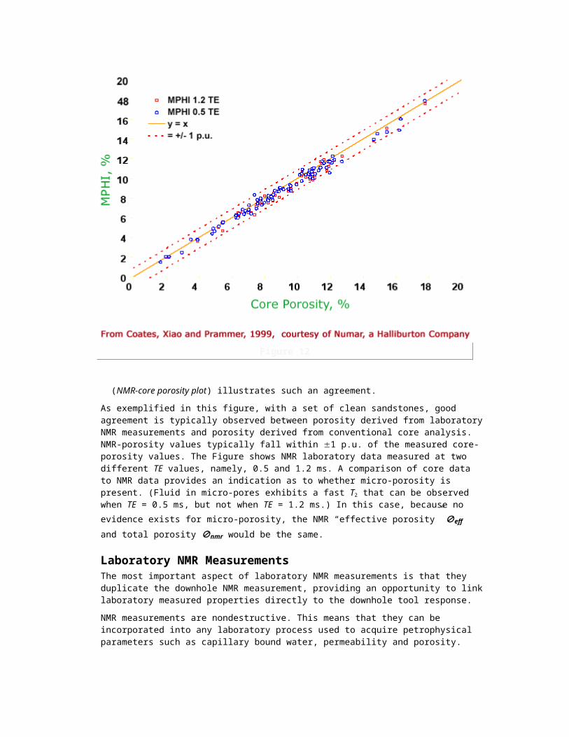
Figure 14

Having estimated the relaxation time cutoff for an enhanced CBVnmr determination, the directly measured core sample permeability can be compared to the NMR permeability model. Using this refined model, a more accurate representation for the downhole measurements can be provided.

Characterize Bulk Fluid Effects to Improve NMR Log InterpretationSelecting the correct data acquisition parameters is vital for accurate, efficient NMR logging. If insufficient recovery time (TW ) is allowed, the resulting porosity will be too low. However wait times that are too long can slow down the downhole logging speeds. Laboratory measurements using different acquisition parameters can be compared with standard core porosity measurements to determine the optimum wait time (TW). An example of this is shown in Figure   15 (Core recovery

time).

Figure 15

Here, we see that if the recovery time is too short, the resulting NMR porosities will be too low. This analysis indicates that a recovery time between 6 and 8 seconds is required to recover all the hydrogen protons for an accurate NMR porosity.

Refine Parameters Needed to Identify and Type HydrocarbonsNMR logging can be used to identify and type hydrocarbons based on bulk relaxation times and diffusion rates. Oil can exhibit a wide range of relaxation times and diffusion constants, most of which are less than bulk water. Hydrocarbon gas has a diffusion mechanism that is significantly greater than water. Laboratory NMR measurements on bulk formation samples can be used to determine the NMR properties of formation hydrocarbons and thus significantly enhance NMR log interpretation.

Figure   16 (Core diffusion effects) shown in both the time domain (top) and the T2 spectrum (bottom),the effects of diffusion can be investigated by changing the spacing of the echoes, which helps determine a fluid’s diffusion constant.

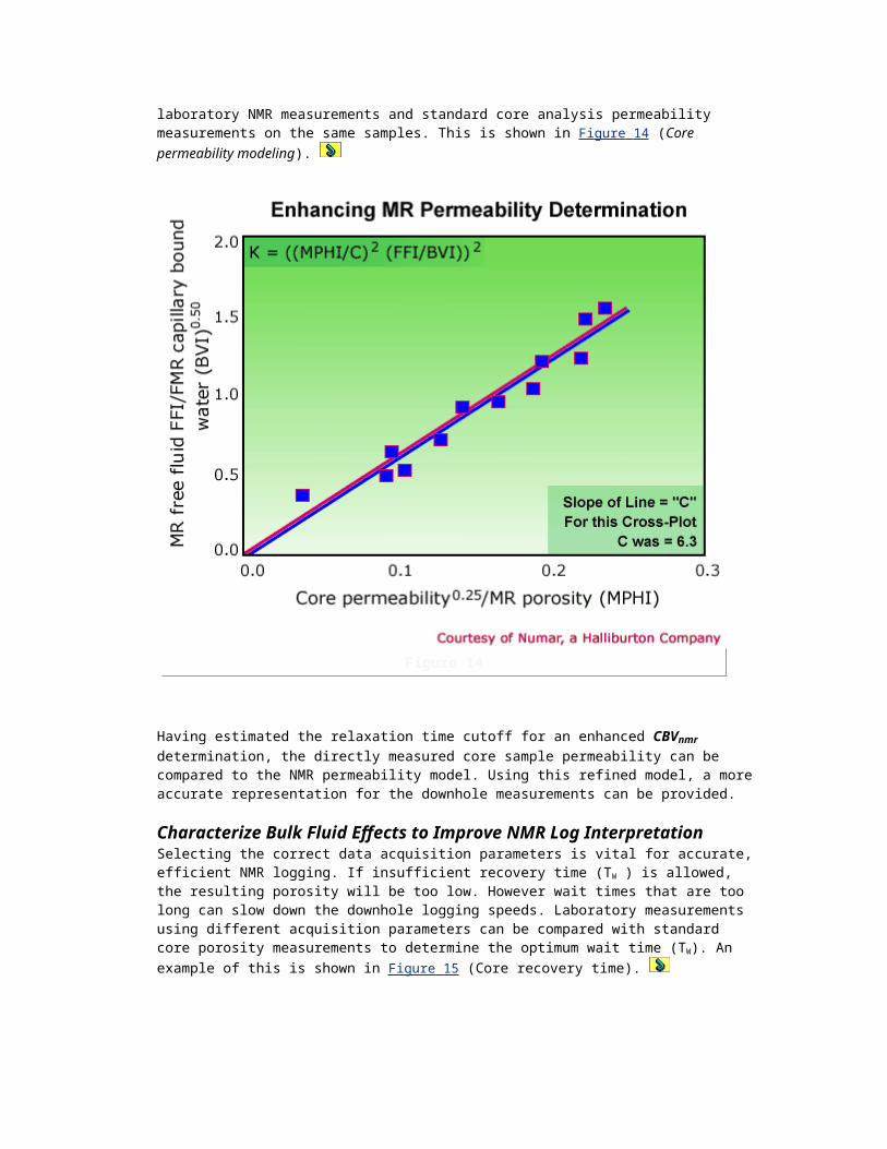
Figure 16

 JOB PLANNING AND LOG QUALITY CONTROL

In this section, we will discuss important issues pertaining to both the CMR and the MRIL logging jobs. We will start with a discussion of planning the job, then move on to quality control, both during and after the log run.

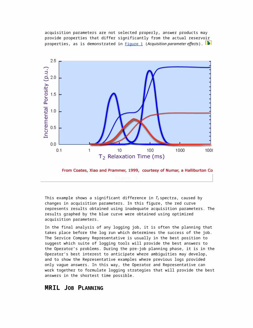
JOB PLANNINGReliable and accurate NMR measurements of reservoir properties require careful, early job planning. Such planning is critical for the success of the logging run. Specific formation and fluid properties can be utilized to design an acquisition scheme that provides access to yet unknown reservoir characteristics, and which optimizes the acquisition process and thus improves the answers derived from the data. If acquisition parameters are not selected properly, answer products may provide properties that differ significantly from the actual reservoir properties, as is demonstrated in Figure   1 (Acquisition parameter effects).

Figure  1

This example shows a significant difference in T2 spectra, caused by changes in acquisition parameters. In this figure, the red curve represents results obtained using inadequate acquisition parameters. The results graphed by the blue curve were obtained using optimized acquisition parameters.

In the final analysis of any logging job, it is often the planning that takes place before the log run which determines the success of the job. The Service Company Representative is usually in the best position to suggest which suite of logging tools will provide the best answers to the Operator’s problems. During the pre-job planning phase, it is in the Operator’s best interest to anticipate where ambiguities may develop, and to show the Representative examples where previous logs provided only vague answers. In this way, the Operator and Representative can work together to formulate logging strategies that will provide the best answers in the shortest time possible.

MRIL JOB PLANNINGA clear definition of the logging objectives is essential in MRIL job planning and preparation. Limited objectives for porosity and permeability measurement can be met using standard data acquisition (activations), which allow easy and relatively fast logging. Supplemental objectives for hydrocarbon typing, however, call for advanced activations, which need to be run at reduced logging speed. Estimates of in-situ conditions are required to judge the applicability of the preferred type of activation, and to optimize the acquisition parameters and enhance the value of the outcome.

MRIL job planning can be executed in three basic steps:

1. Determine NMR fluid properties (T1, bulk, T2, bulk, D0, and HI). This step is straightforward if samples of formation fluid are available. Alternatively, these properties can be estimated from global correlations based on estimated formation conditions.

2. Assess expected NMR responses (decay spectrum, polarization, apparent porosity) over the intervals to be logged. Again these may be estimated from available information on formation and fluid properties. In many cases, only a crude idea of the rock properties is necessary for job planning.

3. Select activation sets and determine appropriate activation parameters for TW, TE, and NE. (This step is covered in greater detail below.)

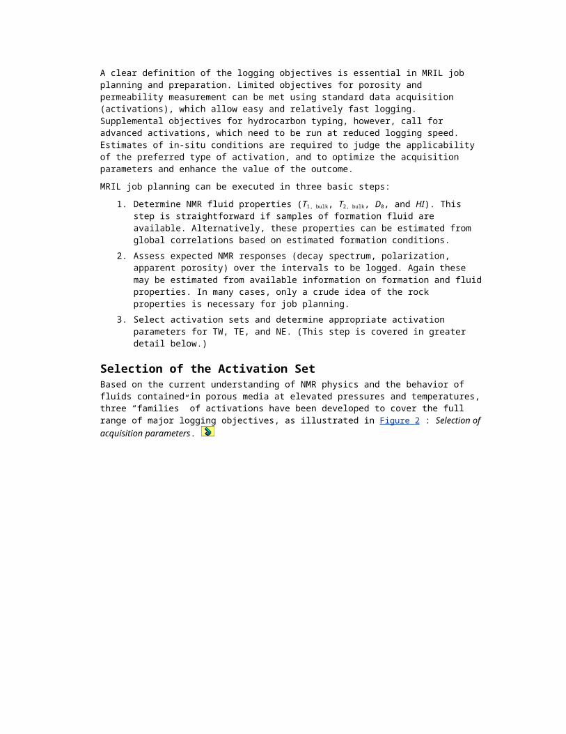
Selection of the Activation Set Based on the current understanding of NMR physics and the behavior of fluids contained in porous media at elevated pressures and temperatures, three “families” of activations have been developed to cover the full range of major logging objectives, as illustrated in Figure   2 : Selection

of acquisition parameters.

Figure 2

Standard T2 activations provide data to determine porosity, permeability, and productivity (mobile fluids).

Dual-TW activations provide data to determine porosity, permeability, and productivity (mobile fluids) and to perform some direct hydrocarbon typing and quantification.

Dual-TE activations require slower logging speeds and provide data to determine porosity, permeability, and productivity (mobile fluids,) and to perform direct hydrocarbon typing, including viscous oil.

CMR JOB PLANNINGFor CMR logging, the following issues should be addressed prior to running the tool in the hole:

What is the objective of running the NMR tool?

What are the accuracy, precision and vertical resolution requirements?

What are the expected properties of the mud and formation fluids?

Mud type,

Hydrocarbon viscosity,

Formation pressure and

Temperature

What is the lithology?

Mineralogy

Texture, pore size and grain size

The answers (or best estimates) to these questions will aid in selecting the best logging parameter values.

LOG QUALITY CONTROL This section describes quality control measures for the Numar and the Schlumberger magnetic resonance logging tools.

NUMAR MRIL LOG QUALITY CONTROLQuality control is essential to obtaining accurate information from the MRIL log. A system of tool-integrity and log-quality indicators is used to assure the highest level of data quality. The MRIL quality-control procedures include calibration before and after the survey, operational set-up, log recording, display of quality indicators, and a final quality check.

MRIL Quality Control During Logging

Logging Speed and Running Average The logging speed of MRIL is affected by many factors. Speed charts, which determine the logging speed, are based on

gain

activation

polarization time

tool type

tool size

desired vertical resolution

operating frequency

Information from the speed chart is essential for selecting the correct (minimum) running average, based on tool gain.

MRIL Log Quality DisplayAll of the quality indicators are recorded in the raw data file, and are available for playback whenever needed. MRIL log quality can be displayed in a variety of formats. All quality indicators should be checked. This is easily achieved, because indicators have certain shadings if their values are outside of their allowable ranges.

Post-MRIL Logging Quality Checks

The MRIL responses should be checked against other logs when available. Two equations are essential for understanding MRIL tool responses and their relationships to petrophysical parameters:

]1[)(

1TTW

eHIMPHI e

CBWMPHIMSIG where

MPHI = effective porosity measured by the MRIL tool

e = effective porosity of the formation

HI = hydrogen index of the fluid in the effective porosity system

TW = polarization time used during logging

T1 = longitudinal relaxation time of the fluid in the effective porosity system

MSIG = total porosity measured by MRIL total-porosity logging

CBW = clay-bound water measured by the MRIL tool with TE = 0.6 ms and partial-polarization activation

Agreement of MPHI with XPHI in Clean, Water-Bearing FormationsIn clean, water-filled formations, MPHI should be approximately equal to XPHI (the density-neutron cross-plot porosity). In shaly sands, MPHI should approximately equal density porosity calculated with the correct grain density.

Knowing the mud type is also essential for analyzing the response of an MRIL tool. Because of the tool’s relatively shallow depth of investigation, the tool investigates primarily the flushed zone.

Effects of Hydrogen Index and Polarization Time on MPHIMPHI may not equal effective porosity because of the effects of both hydrogen index and long T1 components. The MRIL Prime measurement process usually eliminates the porosity underestimation that results from T1 effects. The measurements are still affected by the hydrogen index (HI). In clean gas zones, MPHI values obtained from stationary measurements should be close to neutron porosity values calculated with the correct matrix.

MPHI Relation to MSIG on Total-Porosity LogsMRIL effective porosity (MPHI) is always less than MRIL total porosity (MSIG), except in very clean formations. In the latter case, clay-bound-water porosity (CBW) is zero, thus MPHI equals MSIG. In general, MPHI £ MSIG.

MPHITES Relation to MPHITEL on Dual-TW logsPorosity measured with a short polarization time (MPHITwS) is usually underestimated, and thus will be less than porosity measured with a longer polarization time (MPHITwL). Such is the case even if TWL is not long enough for full polarization. This underestimation is especially prevalent in hydrocarbon-bearing zones. So, in general, MPHITwS £ MPHITwL.

MPHITES Relation to MPHITEL on Dual-TE logsBecause of diffusion effects, a T2 distribution obtained with a long TE will appear to be shifted to the left of a distribution obtained with a shorter TE. Because some of the T2 components may be shifted out of the very early bins, some porosity in the early bins will not be recorded with a long TE. Therefore, in general, MPHITEL £ MPHITES.

 

SCHLUMBERGER CMR LOG QUALITY CONTROLQuality control is essential for obtaining accurate information from the CMR log. Since skid contact with the formation is essential, the CMR tool must be run eccentered.

CMR Quality Control During Logging

Logging Speed and Running Average Maximum logging speeds are automatically calculated by the MAXIS computer, based on the tool’s pulse sequence and sample rate. This maximum logging speed ensures that a new measurement is properly acquired during each sample interval.

CMR Log Quality DisplayAll of the quality indicators are recorded in the raw data file, and are available for playback whenever needed. Field CMR logs include the following log quality controls related to logging conditions:

Bad-hole flag

Insufficient wait time flag

Post-CMR Logging Quality ChecksThe CMR porosity logs should be checked for correct response in the following environments:

Clean, water-saturated formations or formations where the fluid hydrogen index = 1. The CMR porosity is comparable to neutron and density porosities in clean sandstones and carbonates.

Shaly Formations: Free fluid porosity is much lower than CMR porosity in shaly formations

Shales: In shales the CMR free fluid porosity reads low (close to 0 p.u.)

Gas Zones: In clean gas zones, the CMR porosity is much lower than the density porosity and is typically comparable to neutron porosity. The CMR response in gas zones depends on invasion, wait time and the hydrogen index of the gas.

Heavy Oil Zones: CMR porosity does not include the volume of heavy oil (or bitumen). The CMR is lower than neutron and density porosities where heavy oil is present.

 NMR APPLICATIONSThe broad range of data available from the current generation of NMR logging tools enables the tool to be utilized in a variety of applications. The most fundamental of these is the measurement of total porosity, independent of formation type. Directly leading on from this are applications based on analysis of the porosity distribution to provide permeability information and the quantification of producible fluid versus bound fluid. A further range of applications is based on the evaluation of fluid type, differentiating between water, light or viscous oil and gas. These applications are shown in the following sections, using examples obtained by Numar’s MRIL tool and Schlumberger’s CMR tool.

POROSITY AND PERMEABILITY

POROSITY EXAMPLE FROM NUMAR MRIL LOGFigure   1 (MRIL log) presents data from a well that was drilled through a shaly sand in Egypt.

Figure 1

Track 1 contains MRIL permeability (green curve) and core permeability (red asterisks). Track 2 contains MRIL porosity (blue curve), neutron and density porosity (green curves), and core porosity (red asterisks).

In this reservoir, the highly variable grain sizes resulted in considerable variation in rock permeability. Capillary-pressure measurements on rock samples yielded a good correlation between pore bodies and the pore throat structures. This correlation indicates that the NMR T2 distribution provides a good representation of the pore-size distribution when pores are 100% water saturated.

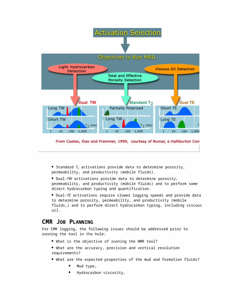
PERMEABILITY EXAMPLE FROM NUMAR MRIL LOGFigure   2 (Australian MRIL log presentation) shows MRIL log data acquired through a massive

sandstone reservoir in Australia’s Cooper basin.

Figure 2

This reservoir exhibits low-porosity (approximately 10 p.u.) and low-permeability (approximately 1 to 100 md).

Track 1 displays gamma ray and caliper curves. Track 2 shows deep-and shallow-reading resistivity logs. Track 3 presents the MRIL calculated permeability and shows core permeability measurements for easy comparison between the two methods. Track 4 shows the MRIL porosity response, neutron and density porosity readings (based on a sandstone matrix), as well as core porosity.

This well was drilled with a potassium chloride (KCl) polymer mud [48-kppm sodium chloride (NaCl) equivalent] and 8.5-in. bit. MRIL data were acquired with TW = 12 seconds and TE = 1.2 ms.

Over the interval depicted, the log shows a clean sandstone formation at the top, a shaly sandstone at the bottom, and an intervening shale between the two sandstones. Agreement between MPHI and the core porosity is good. The slight underestimation of MPHI relative to core porosity is attributed to residual gas within the flushed zone. The MRIL permeability curve was computed using a model customized to this area. The agreement between MRIL permeability and core permeability is very good.

HYDROCARBON TYPING

SCHLUMBERGER CMR LOG EXAMPLE

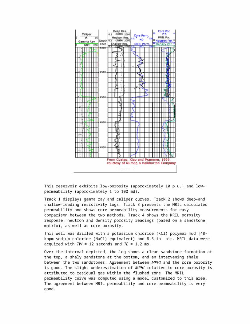
Figure   3 (CMR tar zone) shows how tar zones presented on the CMR log.

Figure 3

In water, gas or oil, the CMR tool has a clear tar signature as seen in Zone C—a suppression of the long T2 components (track 5) and a reduction in total porosity (track 4). In this well, the CMR tool is able to confirm—by the presence of large T2 contributions from oil and no reduction in total CMR porosity—that the lower oil zone (Zone E) is not tar, but mobile oil, which may have been trapped by a local stratigraphic closure.

NMR ENHANCED WATER SATURATION WITH RESISTIVITY DATA

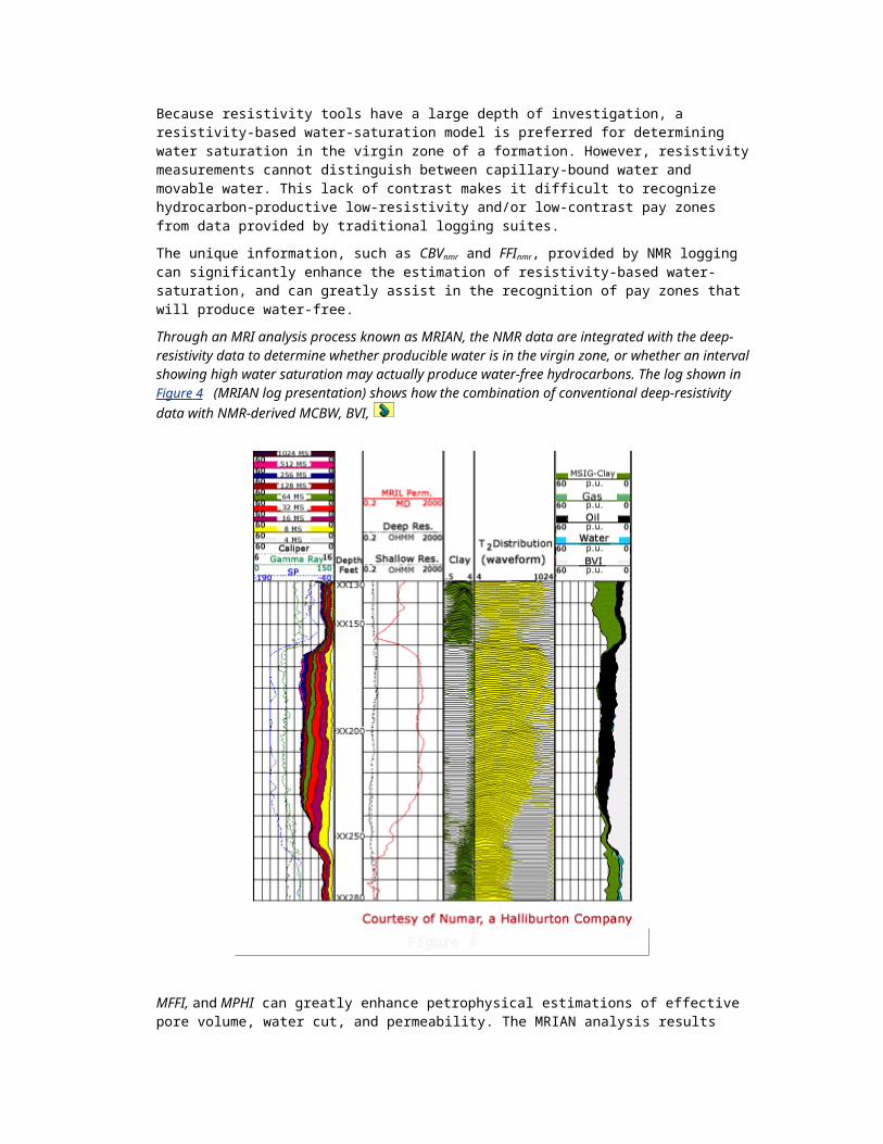
NUMAR MRIL LOG EXAMPLEBecause resistivity tools have a large depth of investigation, a resistivity-based water-saturation model is preferred for determining water saturation in the virgin zone of a formation. However, resistivity measurements cannot distinguish between capillary-bound water and movable water. This lack of contrast makes it difficult to recognize hydrocarbon-productive low-resistivity and/or low-contrast pay zones from data provided by traditional logging suites.

The unique information, such as CBVnmr and FFInmr, provided by NMR logging can significantly enhance the estimation of resistivity-based water-saturation, and can greatly assist in the recognition of pay zones that will produce water-free.

Through an MRI analysis process known as MRIAN, the NMR data are integrated with the deep-resistivity data to determine whether producible water is in the virgin zone, or whether an interval showing high water saturation may actually produce water-free hydrocarbons. The log shown in Figure   4 (MRIAN log presentation) shows how the combination of conventional deep-resistivity

data with NMR-derived MCBW, BVI,

Figure 4

MFFI, and MPHI can greatly enhance petrophysical estimations of effective pore volume, water cut, and permeability. The MRIAN analysis results displayed in Track 5 show that the whole interval from XX160 to XX255 has a BVI almost identical to the water saturation interpreted from the resistivity log. This zone will likely produce water-free because of this high BVI.

TEST ZONE IDENTIFICATION

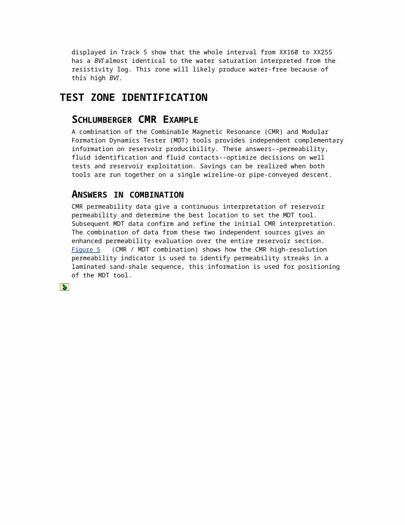
SCHLUMBERGER CMR EXAMPLEA combination of the Combinable Magnetic Resonance (CMR) and Modular Formation Dynamics Tester (MDT) tools provides independent complementary information on reservoir producibility. These answers--permeability, fluid identification and fluid contacts--optimize decisions on well tests and reservoir exploitation. Savings can be realized when both tools are run together on a single wireline-or pipe-conveyed descent.

ANSWERS IN COMBINATION

CMR permeability data give a continuous interpretation of reservoir permeability and determine the best location to set the MDT tool. Subsequent MDT data confirm and refine the initial CMR interpretation. The combination of data from these two independent sources gives an enhanced permeability evaluation over the entire reservoir section. Figure   5 (CMR / MDT combination) shows how the CMR high-resolution permeability indicator is used to identify permeability streaks in a laminated sand-shale sequence, this information is used for positioning of the MDT tool.

Figure 5

Fluid identification Data from CMR, resistivity, density and neutron logs, combined with MDT pressure measurements and fluid samples, yield positive identification of formation fluids. Real-time optical fluid analysis from the MDT tool provides in-situ crude oil typing for estimates of gas-oil ratio, API gravity and coloration. There is minimal contamination before sampling because the OFA Optical Fluid Analyzer module allows uninterrupted monitoring of the flowline fluids and therefore optimal filtrate cleanup. Fluid contact changes in the CMR log reflect the tool’s response to different formation fluids, and the MDT tool provides pressure gradients. These two independent measurements of fluid type confirm gas, oil and water contacts. The CMR bound-and free-fluid answers can be used to determine the best points for obtaining MDT formation pressure measurements and samples.

SINGLE LOGGING RUN One run is eliminated and efficiency is improved when the MDT and CMR tools are combined in one trip, even though they are operated sequentially, rather than simultaneously. Time savings are significant and greatly improve the efficiency of sampling operations. Less time spent in sampling lowers the probability of deteriorating well conditions and stuck tools.

 CASE HISTORIESIn this section, we will see how NMR logs were able to differentiate between productive and non-productive zones in cases where conventional logging suites were unable to properly discern the difference.

LOW-RESISTIVITY-RESERVOIR EVALUATION USING NUMAR’S MRIL TOOL

In this example, we see how Numar’s MRIL data were used to provide a better understanding of reservoir lithology to improve production in a zone that would have otherwise been considered non-productive.

SETTINGThe reservoir penetrated by this well consists of a massive, medium-to fine-grained sandstone formation, developed from marine shelf sediments that were subjected to intense bioturbation. Air permeability typically ranges between 1 and 200 md, with core porosity varying between 20 and 30 p.u.

The upper portion of the reservoir (Zone A) has higher resistivity (approximately 1 ohmm) than that of the lower reservoir (Zone B, approximately 0.5 ohmm). Produced hydrocarbons consist of light oil with viscosity from 1 to 2 cp.

The Operator’s DilemmaThe well was drilled with water-based mud. Conventional logs are shown in Figure   1 : SP,

Resistivity and Neutron/Density logs.

Figure 1

These logs suggest that the upper part of the sand (XX160 to XX185) would possibly produce with a high water cut, but that the lower part of the sand (XX185 to XX257) is probably wet.

The operator was concerned by the decrease in resistivity seen within the lower portion of the reservoir. The operator needed to know whether the decrease was due to

textural changes (smaller grain sizes, in which case the well might produce free of water) or

an increase in the volume of movable water.

The ability to reliably answer this question would make a significant impact on reserve calculations, well-completion options, and future field-development decisions.

An additional piece of important information for this reservoir is that actual cumulative production often far exceeds the initial calculated recoverable reserves, based on a water-saturation cutoff of 60%. If the entire zone in question were actually at irreducible water saturation, then the total net productive interval could be increased from 25 to 70 ft. This gain would result in increased net hydrocarbon pore volume by more than 200%, accompanied by significant increases in expected recoverable reserves.

MRIL logs were incorporated into the logging suite for two principle reasons:

to distinguish zones of likely hydrocarbon production from zones of likely water production by establishing the bulk volume of irreducible water (bvi) and the volume of free fluids (mffi)

to improve the estimation of recoverable reserves by defining the producible interval

MRIL SolutionThe MRIL data acquired in this well included total porosity to determine clay-bound water, capillary-bound water, and free fluids. MRIL results from both TDA and MRIAN are illustrated in Figure   2 : MRIL log presentation.

Figure 2

Dual-TW logging was to be used to distinguish and quantify hydrocarbons. The MRIL data interpretation provided the basis for revising details in the reservoir’s depositional model, and resulted in an improved understanding of this reservoir’s lithology.

Interpretation of MRIL DataMRIL data were acquired in the well and were used in DSM, TDA, and MRIAN analyses. The MRIL data in Figure   2 (MRIL log presentation) helped the Operator to determine that the resistivity reduction was due to a change in grain size and not to the presence of movable water. The two potential types of irreducible water that can cause a reduction in measured resistivity are clay-bound water (whose volume is designated by MCBW) and capillary-bound water (whose volume is indicated by BVI). The MRIL clay-bound-water measurement (Track 3) indicates that the entire reservoir has very low MCBW. The MRIL BVI curve (Track 7) indicates a coarsening-upward sequence (BVI increases with depth). The increase in BVI and the corresponding reduction in resistivity are thus attributed to the textural change. The TDA analysis (Track 6) determined oil saturation in the flushed zone to be in the 35-to-45% range. Results of the TDA (Track 6) and TDA/MRIAN (Track 7) combination analysis imply that the entire reservoir contains no significant amount of movable water and is at irreducible condition. The MRIAN results (Track 7) indicate that both the upper and lower intervals have high water saturation, but

that the formation water is at irreducible conditions. Thus, the zone should not produce any formation water. The entire zone has permeability in excess of 100 md (Track 2). Based on these results, the operator perforated the interval from XX163 to XX234. The initial production of 2,000 BOPD was water-free and thus confirmed the MRIL analysis.

Note the difference between the TDA and TDA/MRIAN results in the MRIL log presentation. The TDA shows that the free fluids include both light oil and water, whereas the TDA/MRIAN results show that all of the free fluids are hydrocarbons. This apparent discrepancy is simply due to the different depth of investigation of the various logging measurements. TDA saturation reflects the flushed-zone as seen by MRIL measurement. The TDA/MRIAN combination saturation reflects the virgin zone as seen by deep-resistivity measurements. Because water-based mud was used in this well, some of the movable hydrocarbons were displaced in the invaded zone by the filtrate from the water-based mud.

EVALUATION OF RESERVOIR PRODUCIBILITY USING SCHLUMBERGER’S CMR TOOL

In this example, we see how Schlumberger’s CMR data were integrated with conventional logging and pressure data to differentiate between gas, oil, and tar within a complex reservoir.

SETTINGThis well was drilled with oil-base mud in eastern Venezuela. In this reservoir, the Operator needed to identify gas, oil and tar zones. The Operator chose a suite of logs which included Schlumberger’s CMR tool in order to successfully determine the producibility of each zone within the reservoir.

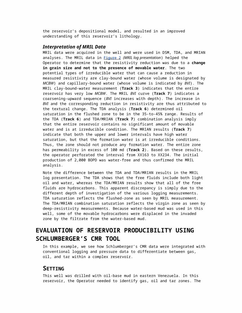
CMR AnswersFigure   3 (Evaluation of CMR reservoir producibility) shows the results from the log run.

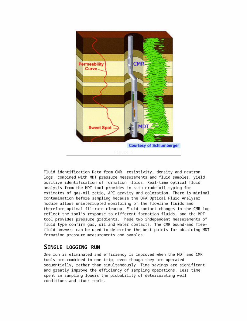
Figure 3

The CMR-MDT log helped to sharply define the fluid types inferred by the density-neutron data. The CMR and density-neutron data confirmed gas in Zones A and H. The other zones had no density-neutron crossover (interpreted as oil), but several zones had a CMR porosity deficit (identified by the blue shading on the log example). The CMR porosity deficit, as compared to the density-neutron porosity, was attributed to the presence of tar in Zones B, D, E, F and I. The resistivity log showed no contrast between the tar and hydrocarbon zones in this oil-base mud environment.

The MDT pressure points independently confirmed the presence of tar. All four pressure tests attempted within the tar zones produced dry test results. In contrast, all pressure points attempted in the gas or light-oil zones produced good pressure and mobility readings. The CMR-MDT data, together with the triple combo data provided a conclusive petrophysical analysis of this complex gas, oil and tar system.

IMPROVED TESTING EFFICIENCY WITH SCHLUMBERGER’S CMR TOOLThis example shows how Schlumberger’s CMR tool was used to identify zones for further testing.

SettingThe Operator was drilling a well in waters offshore of China. Previous logs within this reservoir showed an unconsolidated shaly sand formation with little variation in the resistivity and density-neutron porosity curves. Pressure testing had proven problematic in the past.

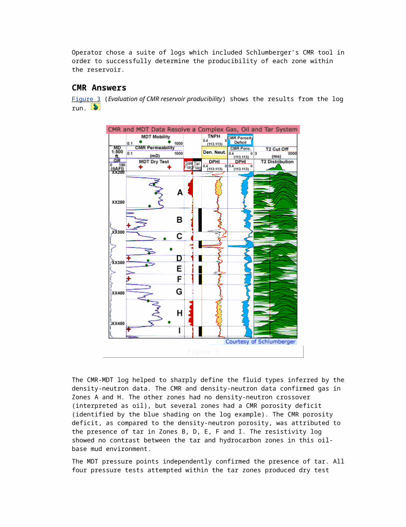
CMR AnswersThe Operator chose to run a CMR tool in order to define permeable zones that would merit further testing (Figure   4 : MDT Test zone identification).

Figure 4

The CMR bound and free-fluid porosity curves showed good definition, and easily identified the more permeable intervals. The MDT points were selected on the basis of the higher permeability areas (low bound-fluid volume), thereby avoiding the low-permeability zones and potential probe plugging.

Six successful pressure tests were obtained, and three samples were recovered in an environment where MDT testing had previously been quite troublesome.

 GLOSSARY OF TERMS

ActivationProgrammed command sequences that control how MRIL tools polarize formations and measure NMR properties of those formations. Activations may contain single or multiple CPMG sequences.

Activation, Dual-TEAn activation that enables the acquisition of two CPMG echo trains at different echo spacings (TE) but at identical re-polarization times (TW). Data acquired with dual-TE activations are used for hydrocarbon identification, and this activation has been successfully used in detecting and quantifying medium-viscosity oils.. The hydrocarbon identification technique takes advantage of

the different diffusivities of the various reservoir fluids. Because the MRIL tool produces a magnetic field gradient, the T2 of each fluid has a component that depends on its diffusivity T2D, and on the TE used in the NMR measurements. Increases in TE will shift the T2 spectrum toward smaller T2 values, and the shift will be different for each fluid type. Separation in T2 space follows

from 12

)( 2TEGD .

Activation, Dual-TWAn activation that enables the acquisition of two CPMG echo trains at different wait times (TW) and identical echo spacings (TE). Data acquired with dual-TW activations are used to improve detection of gas and light oils. This detection is based on the fact that the T1 of gas and light oils is much larger than the T1 of water in a formation.

Polarization p is proportional to TW, i.e., 1

TW

1 Tep

.

The smaller TW is chosen such that the NMR signal from the formation water is completely polarized, but the oil and/or gas signals are not. The longer TW is chosen so that most of the hydrocarbon signals are also polarized. The signal left after the subtraction of the two echo trains or the two resulting T2 distributions contains only signal from the hydrocarbon. This method can be used to quantify oil and gas volumes when the T1 values of oil and gas are known.

Activation, Standard-T2

An activation that enables the acquisition of a CPMG echo train with a TW with which formation fluids can be fully polarized, and with a TE with which the diffusion effects on T2 can be eliminated. Typical values for this activation are TE = 1.2 ms, 3 s £ TW £ 6 s, andNE = 300. This activation is mainly used for determining "effective" porosity and permeability.

Activation, Total-PorosityAn activation that enables the acquisition of two CPMG echo trains with different echo spacings (TE) and different wait times (TW). One echo train is acquired with TE = 0.6 ms and TW = 20 ms (only partial polarization is achieved) and is used for quantifying the small pores which are at least in part associated with clay-bound water. The other echo train is acquired with TE = 0.9 or 1.2 ms and with a TW that is sufficiently long so that full polarization is achieved. This echo train is used to determine effective porosity, and the summation of the two porosities (clay-bound and effective) provides total porosity information. The combination of TE and TW used to acquire the latter echo train constitutes a Standard T2 activation.

B0

Static magnetic field generated by the NMR tool. It may also be designated as Bz.

B1

Oscillating magnetic field generated by a radio-frequency (RF) resonant circuit. This field is applied in the plane perpendicular to B0 and is used to flip the magnetization by 90° and 180°.

BFVCMR Bound fluid volume

Bound WaterA somewhat loosely defined term that can refer either to water that is not producible or to water that is not displaceable by hydrocarbons. Bound water is defined in many references as water that has become adsorbed on the surface of solid particles or grains. Under natural conditions, this water is viscous-like and immobile, but might not have lost its electrolytic properties. Bound water consists of both capillary-bound water and clay-bound water.

Bound Water Saturation (SWB)

The fraction of porosity containing clay mineral associated irreducible water.

Brownian MotionRandom thermal motion of molecules in a fluid

Bulk Volume Irreducible (BVI) The fractional part of formation bulk volume occupied by immobile, capillary-bound water. This bound water is normally not producible, due to capillarity.

Bulk Volume Irreducible, Cutoff (CBVI)BVI is estimated by summing the MRIL T2 distribution up to the time T2cutoff.

Bulk Volume Irreducible, Spectral (SBVI)BVI obtained by the MRIL spectral method. This BVI estimate is determined from a model that assigns a percent of the porosity in each spectral bin to bound water. Various models are available for use with this method.

Bulk Volume Movable (BVM)The fractional part of formation volume occupied by moveable fluids, also referred to as free fluid index (FFI). It can be water, oil, gas, or their combination.

Bulk Volume Water (BVW)The fractional part of formation volume occupied by water. BVW is the product of water saturation and total porosity. Typically expressed as a percentage, it includes clay mineral associated water.

Bz

See B0

Carr-Purcell-Meiboom-Gill Pulse Sequence (CPMG)A pulse sequence used to measure T2 relaxation time. The sequence begins with a 90° pulse followed by a series of 180° pulses. The first two pulses are separated by a time period , whereas the remaining pulses are spaced 2 apart. Echoes occur halfway between 180° pulses at times 2, 4..., where 2 equals TE, the echo spacing. Decay data is collected at these echo times. This pulse sequence compensates for the effects of magnetic field inhomogeneity and gradients in the limit of no diffusion, and reduces the accumulation of effects of imperfections in the 180° pulses as well. Named after the authors of the paper that described this technique: Carr, Purcell, Meiboom and Gill.

CBVI See Bulk Volume Irreducible, Cutoff.

Clay-Bound Water (CBW)Immobile structurally bound water on the surface of clay minerals; the volume of water that is ionically bound to clay minerals present in the formation. Clay surfaces are electrically charged due to ionic substitutions in the clay structure, which allows them to hold substantial amounts of ionically bound water. This water is referred to as water of adsorption or surficially bound water. Clay bound water also includes water of capillary condensation in the micropores in clay aggregates. CBW is a function both of the surface area of the clay and the charge density on its surface. Clay consists of extremely fine particles, so has a very high surface area. CBW contributes to the electrical conductivity of the sand, but not its hydraulic conductivity. Clay-bound water cannot be displaced by hydrocarbons and will not flow. It has very short T1 and T2 times.

CMRThe Schlumberger Combinable Magnetic Resonance tool, follows on from earlier Schlumberger NMR tools that date back to the 1970s. It uses a directional antenna sandwiched between a pair

of bar magnets to focus the CMR measurement on a 6-in. [15-cm] zone inside the formation—the same rock volume scanned by other essential logging measurements. measuring T2 decay components in the 0.1 to 0.5 msec range is possible. These improvements include electronic upgrades, more efficient data acquisition and new signal-processing techniques that take advantage of the early-time information. The CMR is a compact skid tool that is run eccentred. Vertical resolution is 18 inches in standard logging mode, 9 inches in HIRS logging.

CMR-200A later version of the Schlumberger CMR tool

CPMGSee Carr-Purcell-Meiboom-Gill Pulse Sequence

DSee Diffusion Constant.

DIFANSee Diffusion Analysis.

Differential Spectrum Method (DSM)An interpretation method based on dual-TW measurements. DSM relies on the T1 contrast between water and light hydrocarbon to type and quantify light hydrocarbons. The differential spectrum is the difference between the two T2 distributions (spectra) obtained from dual-TW measurements with identical TE. DSM interpretation is performed in the T2 domain.

DiffusionProcess by which molecules or other particles intermingle and migrate because of their random thermally activated (Brownian) motion. Diffusion in a gradient magnetic field causes a reduction in the apparent T2 measured by the CPMG process.

Diffusion Analysis (DIFAN)An interpretation method based on dual-TE measurements. DIFAN relies on the diffusion contrasts between water and medium-viscosity oil to type and quantify oils. The data for DIFAN are acquired through dual-TE logging with a single, long polarization time.

Diffusion Constant (D)Also known as diffusivity. D is the mean square displacement of molecules observed during a period. D varies with fluid type and temperature. For gas, D also varies with density and is therefore pressure dependent. D can be measured by NMR techniques, in particular by acquiring several CPMG echo trains with different echo spacings in a gradient magnetic field.

Diffusion RelaxationA relaxation mechanism caused by molecular diffusion in a gradient field during a CPMG measurement. Molecular diffusion during a CPMG or other spin echo pulse sequence causes signal attenuation and a decrease in the apparent T2. This attenuation can be quantified and the fluid diffusion coefficient measured if a known magnetic field gradient is applied during the pulse sequence. Diffusion only affects the T2 measurement, not the T1 measurement.

Diffusion, RestrictedEffect of geometrical confinement of pore walls on molecular diffusive displacement. NMR diffusion measurements estimate the diffusion constant from the attenuation caused by molecular motion over a very precise time interval. If the time interval (TE in the CPMG sequence) is large enough, molecules will encounter the pore wall or other barrier and become “restricted.” The apparent diffusion constant will then decrease.

Diffusion Limit, FastThe case where protons carried across a pore by diffusion to the surface layer relax at the surface layer at a rate limited by the relaxers at the surface and not by the rate at which the protons arrive at the surface. The diffusion process happens much faster than that of the fluid protons relaxing in a pore. Thus, the magnetization in the pore remains uniform, and a single T1 or T2 can be used to describe the magnetization polarization or decay for an individual pore. This assumption is the basis of the conversion of T1 and T2 distributions to pore-size distributions.

Diffusion Limit, SlowThe case where protons carried across a pore by diffusion to the surface layer relax at the surface layer at a rate limited not by the relaxers at the surface but by the rate at which the protons arrive at the surface. Thus, diffusion does not homogenize the magnetization in the pore space. Multiple exponential decays then are needed to characterize the relaxation process within a single pore.

DiffusivityA measure of the extent to which molecules move at random in the fluid

Direct Hydrocarbon Typing (DHT)A method to determination of the type of hydrocarbons present using MR measurements to exploit the contrast in T1 relaxation and using diffusion principles to recognize fluid types.

Echo Spacing (TE)In a CPMG sequence, the time between 180° pulses. This time is identical to the time between adjacent echoes.

Effective Porosity A somewhat arbitrary term sometimes used to refer to the fractional part of formation volume occupied by connected porosity, and excluding the volume of water associated with clay. It can be thought of as the total porosity less the porosity filled with clay mineral bound water. In NMR logging, the term has usually been associated with porosity that decays with T2 greater than 4 ms.

Effective porosity often refers to the interconnected pore volume occupied by movable fluids, excluding isolated pores and pore volume occupied by adsorbed water. Effective porosity contains fluid that may be immovable at a given saturation or capillary pressure. In petroleum engineering, the term “porosity” usually refers to effective porosity.

For shaly sands, effective porosity is the fractional volume of a formation occupied by only fluids that are not clay bound and whose hydrogen indexes are 1.

Enhanced Diffusion Method (EDM)An interpretation method based on diffusion contrasts between different fluids; used to identify oil and quantify how much is present. A maximum relaxation time for water based on its bulk and diffusion relaxation is computed, so any signal that is observed beyond this time is interpreted as oil. Enhancement of the diffusion effect during echo-data acquisition allows water and oil to be separated on a T2 distribution generated from data acquired with a selected long TE. For typing medium-viscosity oils, EDM uses CPMG measurements acquired through standard T2 logging with a long TE. For quantifying fluids, EDM needs data acquired through dual-TW logging with a long TE or through dual-TE logging with a long TW.

f0

See Larmour frequency.

Free Fluid Index (FFI)The fractional part of formation volume occupied by fluids that are free to flow. A distinction must be made between fluids that can be displaced by capillary forces, and fluids that will be produced at a given saturation. In MRIL logging, FFI is the BVM estimate obtained by summing the T2 distribution over T2 values greater than or equal to T2cutoff.

Free Induction Decay (FID)The transient NMR signal resulting from the stimulation of the nuclei at the Larmor frequency, usually after a single RF pulse. The characteristic time constant for an FID signal decay is called T’2*. T’2* is always significantly shorter than T2.

GaussUnit of magnetic field strength. 10,000 gauss = 1 tesla. The earth’s magnetic field strength is approximately 0.5 gauss.

GradientAmount and direction of the rate of change in space of some quantity such as magnetic field strength.

Gradient Magnetic FieldA magnetic field whose strength varies with position. The MRIL tool generates a gradient magnetic field that varies in the radial direction. Within the small sensitive volume of the MRIL tool, this gradient can be regarded as linear and is usually expressed in Gauss/cm or Hz/mm.

Gyromagnetic Ratio (g)Ratio of the magnetic moment to the angular momentum of a particle. A measure of the strength of the nuclear magnetism. It is a constant for a given type of nucleus. For the proton, = 42.58 MHz/Tesla.

Hydrogen Index (HI)The ratio of the number of hydrogen atoms per unit volume of a material to the number hydrogen atoms per unit volume of pure water at equal temperature and pressure. The HI of gas is a function of temperature and pressure.

Inversion RecoveryA pulse sequence employed to measure T1 relaxation time.

The sequence is 180° -i -90°-Acquisition -TW, where i = 1 … N.

The first 180° pulse inverts the magnetization 180° relative to the static magnetic field. After a

specific wait time (i , the inversion time), a 90° pulse rotates the magnetization into the transverse plane, and the degree of recovery of the initial magnetization is measured. After a wait time TW to return to full polarization, the sequence is repeated. To produce sufficient data for measurement of

T1, this sequence must be repeated many times with different I and thus is very time consuming.

Irreducible Water Saturation (SWIRR)The fraction of the porosity, either total or effective, filled with irreducible water.

I W TInitial wait time

cSee Magnetic Susceptibility

ksdr

SDR model permeability

Ktim

Timur Coates model permeability

Larmor Equation This equation states that the frequency of precession of the nuclear magnetic moment in a magnetic field is proportional to the strength of the magnetic field.

Larmor FrequencyThe frequency at which the nuclear spins precess about the static magnetic field, or the frequency at which magnetic resonance can be excited. This frequency is determined from the Larmor equation.

MNet magnetization vector. See magnetization.

M0

Equilibrium value of the net magnetization vector directed along the static magnetic field.

Magnetic MomentA measure of the magnetic properties of an object or particle (the proton for example) that causes the object or particle to align with the static magnetic field.

Magnetic Resonance (MR)Magnetic resonance describes a group of phenomena more general than NMR. It also includes nuclear quadruple resonance (NQR) and electron paramagnetic resonance (EPR). Because the term nuclear is often related with radioactivity, the term MR is used to avoid this connotation. (NMR means nuclear magnetic resonance, i.e., the term nuclear refers to the magnetic resonance of an atomic nucleus.) Magnetic Resonance Technology uses magnetic fields to influence and measure nuclei spins of hydrogen.

Magnetic Resonance Imaging (MRI)Refers to imaging with NMR techniques. Most MRI machines use a pulsed gradient magnetic field that permits one to localize the NMR signals in space. MRI is used on core samples and in core flooding or flow mechanism studies.

Magnetic Resonance Image Logging (MRIL)The name for the specific NMR logging tool developed by NUMAR Corporation in the mid-1980s. The MRIL tool uses a permanent gradient magnetic field and an orthogonal RF magnetic field (for generating CPMG pulse sequences) to select concentric cylindrical shell volumes for NMR measurements.

Magnetic Susceptibility (c)The measure of the ability of a substance to become magnetized. Differences in magnetic susceptibility of the pore fluids and the matrix cause internal field gradients.

Magnetization (M)A macroscopic vector quantity resulting from the alignment of the nuclear magnetic moment with the static magnetic field. This vector projected into the plane perpendicular to the static magnetic field is known as the transverse magnetization (Mx). Magnetization (T1 ) and transverse magnetization (T2) are the quantities that are observed by NMR.

Magnetization, Longitudinal (Mz)Component of the net magnetization vector along the static magnetic field B0 (or Bz).

MCBWCBW estimate obtained by summing the T2 distribution obtained from partially polarized CPMG echo trains acquired with a TE = 0.6 ms and TW = 20 ms.

MPERMPermeability estimate obtained from MRIL measurements. Many formulas are in use for determining permeability from NMR measurements, the two most commonly used being the Coates equation and the Schlumberger-Doll Research (SDR) equation. According to the Coates equation,

24

BVI

FFI

C

MPHIk

According to the SDR equation,

gemTak 22

4

where T2gemis thegeometric mean of the T2 distribution.

MPHI The porosity estimate obtained by summing the T2 distribution over T2 values greater than or equal to 4 ms, and less than or equal to the highest T2 value in the distribution, e.g., 1024 ms. MPHI is often considered to be equivalent to effective porosity except in the presence of gas filled porosity, or certain fast relaxation pore sizes or fluid types present in the MR measurement space.

MRIL Analysis (MRIAN)An interpretation method that incorporates deep resistivity data and MRIL standard T2 logging measurements to solve the Dual Water Saturation Model and determine hydrocarbon saturation corrected for clay conductivity effects. MRIAN determines water-filled porosity in the virgin zone, which can be compared with the flushed-zone results provided by MRIL stand-alone analysis techniques, such as TDA, EDM, and DIFAN.

MRIL-C ToolNUMAR’s second-generation MRIL tool introduced in 1994. This tool is capable of performing multiple experiments simultaneously (e.g., the MRIL-C has dual-frequency capability, and the MRIL-C+ has triple-frequency capability). The MRIL-C/TP tool, which was introduced by NUMAR in 1996, provides an estimate of total porosity as well as effective porosity. The C/TP tool is able to measure total porosity because the tool can utilize a reduced TE (0.6 ms). Furthermore, because the tool experiences reduced ringing, the first echo contains valuable information.

Because MRIL-C tools operate in either dual-or triple-frequency mode, successive measurements at different frequencies can follow one another more quickly. Each MRIL frequency excites a signal from a different physical location and thus it is not necessary to wait for repolarization to occur in one location before making a measurement in another location. Alternating between frequencies allows more measurements to be made in a given time, thus permitting logging speed to be increased without reducing S/N, or permitting S/N to be increased without reducing logging speed.

MRIL Depth of InvestigationA term which describes how far into the formation that the MRIL signal can penetrate to provide meaningful formation evaluation measurements. Because the Larmor frequency is a function of B0

and B0 is radially dependent, the Larmor frequency is also radially dependent and thus defines the depth of investigation of the MRIL tool. Furthermore, because B0 is also temperature dependent, it follows that the Larmor frequency, and thus the depth of investigation, are also temperature dependent when a fixed B1 frequency is used, which is always the case. As the temperature of the magnet increases, B0 decreases and the depth of investigation decreases accordingly (e.g., a depth of investigation of about 16 in. at 25ºC decreases to about 14 in. at 150ºC). The variation of depth of investigation with temperature for MRIL tools is discussed and displayed in NUMAR literature and charts.

MRIL-Prime Tool

NUMAR’s latest generation of MRIL tool introduced in 1998. This tool is capable of performing multiple experiments at up to nine frequencies. By alternating between nine frequencies, measurements can be made at a very much higher rate. The MRIL-Prime provides measurements of clay-bound water, effective porosity, capillary-bound water, and hydrocarbon typing in just one pass. Besides saving time, acquiring all the data in one pass eliminates depth-shift errors.

The MRIL-Prime tool has additional pre-polarization magnets placed above and below the antenna that allow for full polarization of the fluids. This pre-polarization design can provide 12 seconds of polarization at logging speeds as high as 24 ft/min. Furthermore, the capability of the tool to fully polarize fluids at high logging speeds, and obtain a full T2 distribution without any corrections, makes the logging results much less sensitive to certain job-design parameters.

Planning logging jobs for earlier tools required some knowledge of the time needed to polarize fluids. The MRIL-Prime tool can simply handle the longest polarization times without reducing logging speed. Thus, this tool can be run much like standard triple-combo tools—just run the tool to the bottom of the hole and log up without special passes in the hole and without having to subsequently assembly data from different passes. This is why the MRIL-Prime tool is the first NMR device that can realistically be considered a “primary formation evaluation” logging tool.

MRIL Sensitive-Volume ThicknessThe thickness of the zone for which the MRIL tool provides information The thickness of the sensitive volume for the MRIL tool is approximately 1 mm, and is a function of the gradient strength of the B0 field and the frequency band of the B1 field.

MSIGPorosity estimate obtained by combining data from dual-TE logging with TE = 0.6 and 1.2 ms. MSIG should agree well with total porosity measured on cores. MSIG = MCBW + MPHI. Provides total volume of fluids in the formation.

Mud DopingThe practice of adding magnetite to the drilling mud. With the now obsolete NML tool, doping was essential to kill the borehole signal. However, doping the mud with a paramagnetic substance to change the NMR properties of invading mud filtrate may still be desirable. For instance, if the invaded zone is flushed with paramagnetic ions, then the bulk relaxation time of the brine is shortened, and water signals are killed. Thus, only oil signals remain, and residual oil saturation can be determined through NMR measurements. MnCl2, has recently been shown to be a cost effective doping agent for this application.

MWTMulti-wait time

Mx

See Transverse Magnetization.

Mz

See Longitudinal Magnetization.

NENumber of echoes in a CPMG echo train.

NML Tool The original Schlumberger Nuclear Magnetic logging tool, developed in the 1970’s. Now an obsolete NMR logging tool that utilized the earth’s magnetic field. The NML tool measured the precession of hydrogen protons in the earth’s magnetic field after the alignment of protons with a superimposed magnetic field. The sensitive volume of the NML was not a thin cylindrical shell, but a full cylinder centered around the tool; therefore, the measurement contained borehole signals.

Operation of the NML required special doping of the borehole fluids to eliminate the signal from the protons in the borehole.

Non-Effective Porosity The difference obtained by subtracting effective porosity from total porosity (effective porosity is equal to the MPHI measurement on the MRIL log, and total porosity is equal to the MSIG measurement on the MRIL log). Non-effective porosity represents that segment of porosity which will not be produced; this is the part which would hold bound water.

Nuclear Magnetic Resonance (NMR) NMR, as a physical phenomenon, is the absorption or emission of electromagnetic energy by nuclei in a static magnetic field, after excitation by a stable RF magnetic field. NMR, as an investigative tool, is a method that uses the NMR phenomenon to observe the static and dynamic aspects of nuclear magnetism. The method requires a static magnetic field to orient nuclear magnetic moments, and an orthogonal oscillating field (at RF frequencies) to excite the nuclear magnetic moments. The frequency of the oscillating field must satisfy the Larmor resonance condition.

NMR can be used to detect molecular structures and probe molecular interactions. It is a major chemical spectroscopic technique with many applications, including probing properties of fluids in porous media.

Despite the term nuclear, NMR does not involve radioactivity.

NWTNumber of wait times.

P1

Amplitude value on the T2 distribution.

PAPPhase-alternated pair

Paramagnetic MaterialsMaterials with a small but positive magnetic susceptibility. The addition of a small amount of paramagnetic material to a substance may greatly reduce the relaxation times of the substance. Most paramagnetic substances posses an unpaired electron and include atoms or ions of transition elements (e.g., manganese and vanadium) or rare earth elements. Oxygen (O2) is also paramagnetic and contributes to the relaxation of water. Paramagnetic substances are used as contrast agents in medical MR imaging and to dope the borehole fluids in some applications of NMR logging. Copper sulfate (CuSO4) is used to dope the water in a calibration tank to reduce water relaxation times, thereby significantly reducing MRIL calibration time.

Phase Alternate Pairs (PAP)A method of acquiring two echo trains that are 180° out of phase. The change in echo-train phase is accomplished by changing the phase of the initial 90° pulse in the CPMG sequence by 180°. The effect of this change is to reverse the sign of the echo data. In processing, the two echo trains are subtracted to eliminate the effects of ringing and baseline offset.

Permeability, Absolute A measure of the ability of a rock to conduct a fluid or gas through its interconnected pores when the pores are 100% saturated with that fluid. Measured in darcies or millidarcies (md).

Permeability, EffectiveThe capability of a rock to conduct a fluid in the presence of another fluid, immiscible with the first, is called its effective permeability to that fluid. Effective permeability not only depends on the permeability of the rock itself, but also on the relative amounts of the different fluids in the pores.

Permeability, Relative The ratio between the effective permeability to a given fluid at a partial saturation and the permeability at 100% saturation. Relative permeability is the ratio of the amount of a specific fluid that will flow at a given saturation, in the presence of other fluids, to the amount that would flow at a saturation of 100%, other factors remaining the same.

Polarization Time (TW)See Wait Time.

Porosity, Effective (e )A somewhat arbitrary term sometimes used to refer to the fractional part of formation volume occupied by connected porosity and excluding the volume of water associated with clay. In NMR logging, the term has usually been associated with porosity that decays with T2 greater than 4 ms.

Effective porosity often refers to the interconnected pore volume occupied by movable fluids, excluding isolated pores and pore volume occupied by adsorbed water. Effective porosity contains fluid that may be immovable at a given saturation or capillary pressure. In petroleum engineering, the term “porosity” usually refers to effective porosity.

For shaly sands, effective porosity is the fractional volume of a formation occupied by only fluids that are not clay bound and whose hydrogen indexes are 1.

Porosity, TotalThe total pore volume occupied by fluids in a rock. Includes isolated non-connected pores and volume occupied by adsorbed, immobile fluids. For a shaly sand formation, total porosity is the fractional part of formation volume occupied by both clay-bound and non-clay-bound fluids.

PrecessionThe motion of the axis of a spinning body so as to trace out a cone. It is caused by the application of a torque tending to change the direction of the rotation axis. The precession of the proton spin axis about the B0 field axis occurs at the Larmor frequency.

ProtonA positively charged elementary particle that provides the charge in an atomic nucleus. A hydrogen nucleus contains one proton. The symbol 1H is used to designate the hydrogen nucleus.

Proton DensityThe concentration of mobile hydrogen atoms per unit volume. NMR data can be corrected for hydrogen density changes by dividing the apparent NMR porosity by the appropriate hydrogen index.

Pulse, 90°An RF pulse designed to rotate the net magnetization vector 90° from its initial direction in the rotating frame of reference. If the spins are initially aligned with the static magnetic field, this pulse produces transverse magnetization and free induction decay (FID).

Pulse, 180°An RF pulse designed to rotate the net magnetization vector 180° in the rotating frame of reference. Ideally, the amplitude of a 180° pulse multiplied by its duration is twice the amplitude of a °pulse multiplied by its duration. Each 180° pulse in the CPMG sequence creates an echo.

Pulse, HardA term used to describe a high-power, short-duration RF pulse used in NMR pulse sequences. In contrast, soft pulses are usually low-power, long-duration RF pulses. Hard pulses are usually rectangular-shaped in the time domain, and excite wide frequency bands often extending beyond the desired resonance frequency. Hard pulses generally make good use of available RF power,

but exhibit poor frequency selectivity. Because of the narrower pulse widths, hard pulses are more suitable for pulse sequences that require short echo spacing (TE). See “Pulse Shaping” for frequency selectivity.

Pulse ShapingThe amplitude, shape, and width of RF pulses define the frequency selectivity of an NMR measurement (see also Hard Pulse and Soft Pulse). Soft pulses are shaped to improve their frequency selectivity as well as other parameters. How shaping brings about these improvements can be easily understood by taking the Fourier transform of RF pulses. A hard pulse is rectangular in shape and excites a wide range of frequencies far from the main lobe. Thus, the frequency selectivity of a hard pulse is poor. A soft pulse has a greater spread in the time domain, but excites a narrow, uniform range of frequencies. Thus, the frequency selectivity of a soft pulse is good. Soft pulses are essential for MRI and also are very important for the MRIL tool because they allow multiple frequencies to be closely spaced.

In a gradient B0 field, such as the magnetic field produced by the MRIL tool, both the gradient strength and the frequency band of the soft pulse determine the sensitive volume.

Pulse, SoftLow-power, long-duration RF pulses used in NMR measurements. Soft pulses in time domain are rectangular pulses in frequency domain. In medical MRI applications, a soft 90° pulse typically has a width of a few milliseconds. Although soft pulses need not conform to a particular shape, soft pulses usually have crafted pulse envelopes, e.g., truncated Sinc pulses (bell-shaped envelopes), to improve frequency selectivity. See pulse shaping for frequency selectivity

Radio Frequency (RF)Electromagnetic radiation at a frequency in the same general range as that used for radio transmissions. The Larmor frequency for 1H is typically in this range. For an MRIL tool, the Larmor frequency is in the range of 580 to 750 KHz.

Regularization The process used to stabilize the inversion from the measured NMR decay to the NMR spectra. There are many methods in use, of which MAP is one. They all result in a smoothed spectra which varies depending on the method and amount of regularization. The need to use regularization means that there is no unique NMR spectra or pore distribution. In most cases, the major features of the spectra are independent of the method of regularization.

RelaxationThe return of nuclear spins to their equilibrium positions after excitation. In NMR measurements, protons are oriented by an oscillating magnetic field . When this oscillating field is removed, the protons begin tipping back to align with the static magnetic field. In NMR terminology, this tipping back motion is called relaxation, and measurement of the ‘relaxation time’ is the fundamental measurement of NMR logging tools.

Relaxation TimeA time constant associated with the return of nuclear spins to their equilibrium positions after excitation. Several relaxation times are defined in NMR measurements. Each is related to different molecular interaction mechanisms. The most frequently measured relaxation times are T1 and T2. For bulk water, T1 and T2 are approximately 3 seconds. The relaxation times of water in rocks are much smaller and are generally less than 300 ms.

Relaxation Time, Bulk FluidThe relaxation produced by interaction of the fluid with itself. For most cases of interest T1 and T2 are equal. For gas, however, because the diffusivity of gas is much higher than that of liquids, the apparent T2 of gas measured by CPMG technique in a gradient magnetic field can be much smaller than T1.

Relaxation Time, Longitudinal (T1 )Longitudinal, or spin-lattice, relaxation time. This time constant characterizes the alignment of spins with the external static magnetic field. Time for nuclei to align with the static magnetic field.

Relaxation Time, Transverse(T2)Transverse, or spin-spin, relaxation time. The time constant that reflects the rate of transverse energy loss, through spin-spin relaxation, that was created by a perturbing radio frequency pulse. This time constant characterizes the loss of phase coherence that occurs among spins oriented at an angle to the main magnetic field and that is due to interactions between spins. T2 never exceeds T1. Both T2 and T1 have been successfully related to petrophysical properties of interest, such as pore size, surface-to-volume ratio, formation permeability, and capillary pressure.

Residual OilOil remaining in the reservoir rock after the flushing or invasion process, or at the end of a specific recovery process or escape process.

ResonanceVibration in a mechanical or electrical system caused by a periodic stimulus, with the stimulus having a frequency at or close to a natural frequency of the system.

RingingThe oscillatory response of a magnet to the application of high-energy RF pulses. When the MRIL RF antenna is energized with high-energy RF pulses, the MRIL magnet resonates or “rings.” The MRIL magnet acts like a piezoelectric crystal, generating an acoustic oscillating voltage that interferes with the formation signal. Ringing is frequency dependent, and each magnet has a different ringing window (typically 20 to 40 kHz wide) where the ringing effect is smaller than at other frequencies. The ideal operating frequency is one that is located in the middle of a broad ringing window.

Running AverageThis represents the total number of individual experiments (i.e., complete echo trains) needed to produce a high signal-to-noise. Because the PAP technique is used during a CPMG measurement, the Running Averaging is at least two.

SBVISee Spectral Bulk Volume Irreducible

Shifted Spectrum Method (SSM)An interpretation method based on dual-TE measurements with identical TW. The SSM relies on the diffusivity contrast between fluids with different diffusivity to type viscous hydrocarbons. The shifted spectrum refers to the observation of the T2 distribution shifted to smaller T2 values when TE is increased. Gases have much higher diffusivity than oil or water, and are more sensitive to the echo spacing (TE) changes. Heavy oils have very low diffusivity, and are least sensitive to TE changes. The SSM is performed in the T2 domain and uses the difference in the shift between fluids of different diffusivity to identify fluids.

Signal AveragingA method of improving signal-to-noise ratio by averaging echo trains

Signal-to-Noise Ratio (S/N)The ratio of signal amplitude to noise amplitude. Signal refers to the desired part of a detected signal; noise refers to the remainder of the detected signal and includes random noise. S/N is a measure of data quality. The S/N of NMR measurements can be improved by averaging several echo trains, by sampling larger volumes, or by increasing the strength of the B0 magnetic field. If the noise is random (statistical) noise only, then averaging n measurements improves S/N by n1/2.

SpinIntrinsic angular momentum of an elementary particle or system of particles, such as a nucleus. Spin is responsible for the magnetic moment of the particle or system.

Spin EchoReappearance of an NMR signal after the FID has disappeared. A spin echo is the result of the effective reversal of the dephasing of the nuclear spins. After spins are excited by an RF pulse, the spins experience FID because of B0 inhomogeneities. Spin isochromats, which are groups of spins precessing at exactly the same Larmor frequency, lose phase coherence during FID. However, during this decay, the isochromats do not experience many spin-spin interactions and still retain phase memory. If a second pulse (180º) is applied at time after the first RF pulse, the spin isochromats will re-phase in the same amount of time . A macroscopic signal (the spin echo) then occurs at precisely TE = 2. Even if the second pulse is not a 180º pulse, a spin echo can still be observed, but this echo will be of smaller amplitude. A third pulse will repeat the process.

Stimulated EchoThe echo formed after magnetization evolves first in the x-y plane, then in the z direction, and again in the x-y plane. A stimulated echo is observed after a three-pulse sequence. Because of B1 inhomogeneities, stimulated echoes occur during CPMG sequences used on logging tools at the same times as regular echoes and must be compensated for through calibration.

Surface Relaxivity (r)A measure rof the capability of a surface to cause protons to relax, i.e., lose orientation or phase coherence. This quantity depends on the strength of fluid-matrix interactions. It also varies with the wettability of the rock surface. Surface relaxation strength r falls in the range of approximately 0.003 to 0.03 cm/s for clastics. r is smaller for carbonates.

T1

See Longitudinal Relaxation Time.

T1effectFraction of gas polarized during the wait time

T1, gas

T1 of gas.

T1/T2

Polarization correction parameter

T2

See Relaxation Time, Transverse.

T2cutoff

A value of T2 that is empirically related to the capillary properties of the wetting fluid in a rock. It is used to differentiate different pore sizes and quantify the amount of bound water. Typically, porosity associated with T2 values less than approximately 33 milliseconds (T2cutoff = 33 ms) are summed to obtain BVI for clastics and, similarly, T2cutoff of approximately 90 ms for carbonates. Note that these values are empirical and may be rock specific.

T2D

Time constant that describes the decay of transverse magnetization caused by molecular diffusion in a gradient field during a CPMG measurement.

T2LM

Logarithmic mean T2

T2S

Time constant that describes the contribution of surface relaxivity to the transverse relaxation time of fluid in a rock. When a single wetting fluid covers the pore surface, T2S dominates the relaxation process. Thus, T2 is proportional to (S/V)-1 of a pore, where S/V is the surface-to-volume ratio. If a spherical pore is assumed, T2 is proportional to the pore radius.

T2*Time constant characterizing the loss of phase coherence that occurs among spins oriented at an angle to the main magnetic field, and that is due to a combination of magnetic field inhomogeneity and magnetic interaction. T2* is always much shorter than T2.

TCP

Carr-Purcell time

Time Domain Analysis (TDA)An important tool used to identify fluid types and calculate saturations through processing of T1-weighted echo differences in the time domain. An alternate method to the differential spectrum method for processing dual-TW echo trains, this interpretation is performed in the time domain rather than in the T2 domain. The key features of the TDA are

subtraction of the two echo trains from one another.

processing the echo differences in the time domain using predicted or measured oil, gas, and water relaxation times and hydrogen-index values

In the DSM, the dual-TW echo trains are first inverted into T2 spectra and subtracted from one another. The interpretation is done in T2 spectrum domain. The effect of T2 spectrum broadening because of noise and regularization smears the partial porosities into adjacent bins, and the subtracted spectrum may contain negative amplitudes that are obviously incorrect. The TDA method has fewer problems with the noise-induced T2 spectrum broadening, and because fewer free parameters need to be determined, the solution is more stable. However, subtracting echoes reduces S/N.

TEThe time between echoes See Echo Spacing.

Total PorosityThe non-solids percentage of rock bulk volume.

Transverse Magnetization (Mx)Component of the net magnetization vector at right angles to the static magnetic field.

TWSee Wait Time.

ViscosityResistance of a fluid to flow. Viscosity is due to internal friction caused by molecular cohesion in the fluid. The diffusion constant D is inversely proportional to viscosity.

Wait Time (TW)The time between the last CPMG 180° pulse and the first CPMG pulse of the next experiment at the same frequency This time is the interval during which magnetic polarization or T1 recovery takes place; the time needed to allow a specific number of nuclei to recover their realized state. Also know as polarization time, this parameter is dependent upon the T1 relaxation of the involved pore sizes and their fluids.

Water WetA solid surface is water wet when the adhesive attraction of water molecules for the solid substance is greater than the attraction between water molecules, i.e., adhesive force > cohesive force.

WettabilityThe capability of a solid surface to be wetted when in contact with a liquid. A liquid wets a solid surface when the surface tension of the liquid is reduced so that the liquid spreads over the surface. Only the wetting fluid in a rock pore has a surface relaxation mechanism. Therefore, wettability affects the NMR properties of fluids in reservoir rocks.

cSee Surface Relaxivity.

GLOSSARY REFERENCESThe definitions used in this section can be found in the following publications:

Glossary of Magnetic Resonance Imaging Terms, in Bushong, S.C., Magnetic Resonance Imaging, Physical and Biological Principles, Second Edition, Mosby, 1996.

Glossary of Terms and Expressions Used in Well Logging, Second Edition, SPWLA, Houston, 1984.

NMR Terminology Glossary, Western Atlas, 1996.

CMR Users guide, Schlumberger, 1997.

 

Spontaneous Potential Log

INTRODUCTIONThe Spontaneous Potential was one of the first logging measurements ever made. It was discovered by accident, appearing as a direct current (DC) potential in the borehole that caused perturbations on the old electric logging systems. The spontaneous potential (SP) curve records the naturally occurring electrical potential (voltage) produced by the interaction of formation connate water, conductive drilling fluid, and shale. The SP curve reflects a difference in the electrical potential between a movable electrode in the borehole and a fixed reference electrode at the surface, as depicted in Figure   1: Spontaneous Potential Configuration. Its usefulness was soon realized, and it is one of the few well log measurements to have been in continuous use for so many years.

Figure 1

Though the SP is used primarily as a lithology indicator and as a correlation tool, it has other uses as well:

permeability indicator,

shale volume indicator (see Vsh calculation in the next section),

porosity indicator, and

measurement of Rw (hence formation water salinity).

Figure   2 shows a typical SP log, with the SP recorded in track one.

Figure 2

Opposite shales, the SP readings are usually fairly constant and tend to follow a straight line, called the Shale Base Line. Opposite permeable formations, the SP shows excursions from the shale base line and drifts to one or more Sand Line levels. (Depending on the relative salinities between the formation water and the mud filtrate, the excursions may be to the left or the right of the shale base line.) This SP effect is produced by two components: the electro-chemical and the electro-kinetic potentials. The SP log is measured in millivolts (abbreviated mV). Notice that there is no absolute scale in mV, only a relative scale of so many mV per division.

When mud filtrate salinities are lower than connate water salinities (i.e., Rmf is > Rw), the SP

deflects to the left (the SP potential is negative). This is called a normal SP. When the salinities are reversed (i.e., salty mud and fresh formation water, Rmf < Rw), the SP deflects to the right.

This is called a reverse SP. Other things being equal, there is no SP (and no SP deflection) at all when Rmf = Rw.

It is quite common to find fresh water in shallow sands and increasingly saline water as depth increases. Such a progression is shown in Figure   3, where the SP appears to be deflecting to the

left deep in the well, but is reversed nearer the surface.

Figure 3

In sand A, we see that Rw is less than Rmf; which means that formation water is saltier than the

mud filtrate. In sand B, the SP deflection is less than in sand A and thus a fresher formation water is indicated. In sand C, the SP is reversed, indicating that formation water is fresher than the mud filtrate and thus Rw is greater than Rmf. Somewhere in the region of 7000 feet it may be guessed

that Rmf and Rw are equal.

RECORDING THE SPThe SP can be recorded very simply by suspending a single electrode in the borehole and measuring the voltage difference between the electrode and a "ground" electrode (often called a "fish"), making electrical contact with the earth at the surface. A generalized illustration of the SP recording system is shown in Figure   4. SP electrodes can be integrated into many logging tools. For example, the SP can be recorded together with an induction log, a laterolog, a sonic log, and a sidewall core gun, once there is conductive mud in the hole. It is important to point out that the SP cannot be recorded in oil-base muds, which allow no conductive path.

THE ELECTROCHEMICAL COMPONENTThe electro-chemical component Ec consists of the liquid junction potential (Ej) and the membrane potential (Em). These potentials create a current that flows at the shale / reservoir interface. When a reference electrode is moved across this interface a difference in potential is measured.

Liquid Junction Potential

We’ve stated that the SP is affected by formation water salinity. When solutions of differing concentration are brought into contact, ions from the solution with a higher concentration tend to migrate toward the solution of lower concentration until equilibrium occurs (Figure   5).

Figure 5 .

However, with sodium chloride (NaCl) solutions, the C1- anions move faster than Na+ cations, so a conventional current (or potential) flows from the less concentrated solution to the more concentrated solution. The electrical potential that results from the combined sodium and chlorine ion movement is known as the liquid junction potential (Elj).

In terms of the solutions present in a formation, mud filtrate can be substituted for the less concentrated solution and formation water will be the more concentrated solution. Borehole mud-weight is usually higher than the formation fluid pressure. This produces an over-pressure at the face of the reservoir exposed to the borehole, and causes mud filtrate to invade the reservoir. A mudcake is subsequently formed and the invasion process slows down. An invasion profile as shown in Figure   6: Liquid Junction Potential is formed which separates, in this case, a high saline formation water and the low salinity mud filtrate.

Figure 6

The liquid junction potential Ej is created at the interface between the invaded zone and the uncontaminated zone due to a salinity difference between mud filtrate and formation water. Since the negative Cl - anions (assuming an NaCl solution) have a greater mobility than the positive Na+ cations, the net result is a flow of negative charges (Cl - ions) from the more concentrated solution to the less concentrated solution. This mechanism, which is driven by the conductivity difference the mud filtrate and formation water is also shown by the above Liquid Junction Potential graphic. The greater the contrast in salinity between mud filtrate and formation water, the larger this potential (Figure   7 ).

Figure 7

Membrane PotentialAnother "battery" found in the formation arises from the molecular construction of shale beds. Shale can act as an ionic sieve or membrane. This means that shale can be permeable for one type of ion while acting as a barrier for another type. This property is called ionic perm-selectivity, and the result is that the shale-membrane can preferentially prevent the movement of negative ions. In this case, shales are permeable to Na+ ions, but not so permeable to C1- ions.

Shales are cation exchangers; they are electro-negative, and therefore repel anions. This phenomenon occurs as a result of the crystalline structure of clay minerals. Their exterior surfaces exchange sites where positively charged cations cling temporarily. In most instances, the shales are 100% effective and therefore repel all chlorine (negatively charged) ions. The positive sodium ions move toward the lower salinity mud in the borehole, but the chlorine ions cannot follow this movement.

Since Na+ ions effectively manage to penetrate through the shale from the saline formation water to the less saline mud column, a positive potential is generated toward the low-concentration NaCl solution of the mud column. This potential is known as the membrane potential (Em). Figure   8

indicates the process.

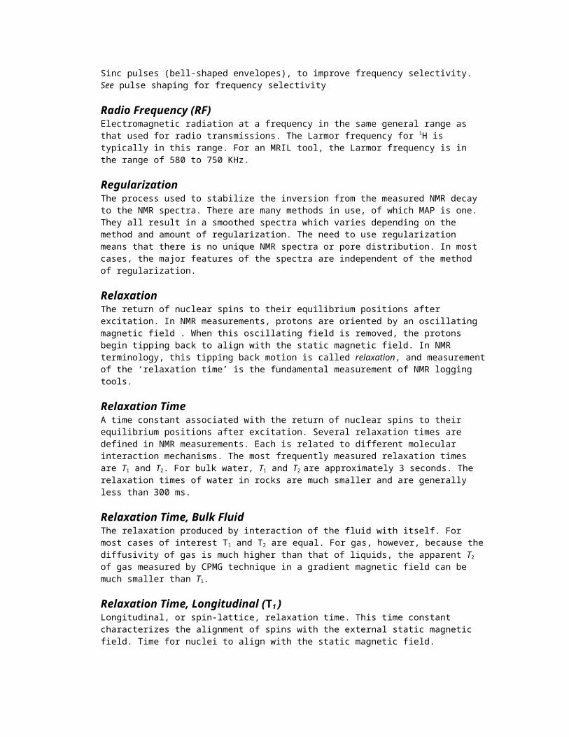
Figure 8

The membrane potential Em acts across the shale between the uncontaminated zone in the reservoir and the mud in the borehole, as depicted in Figure   9: Membrane Potential. This same surface conductance effect manifests itself in the electrical behavior of shaly sands.

Figure 9

TOTAL SPThe total SP (Figure   10) can now be appreciated as the sum of the two components:

Figure 10

[E-1] 

Etotal = Elj + Em 

The total potential, measurable in the borehole by an electrode, is also referred to as the electrochemical component of the SP.

Considering the shale/reservoir interface, a current is created by the Ej and Em potentials acting in series. Ej has a positive value toward the uncontaminated zone containing formation water. In contrast, Em is positive toward the mud in the borehole, which has the lower NaCl concentration.

The magnitude of both the liquid junction potential and the membrane potential depends on the difference in ion concentration between the mud (filtrate) and the uncontaminated formation water, and can therefore both be expressed as:

[E-2] 

mf

w

Con

ConlogKE

 in which K is a constant that varies with temperature (see equation below), while Conw and Conmf are the ion concentrations in the formation water and the mud filtrate respectively that produce the Ej and Em potentials. Conw and Conmf are inversely proportional to the resistivity, Rw of the formation water and Rmf the resistivity of the mud filtrate respectively.

K can be estimated from the temperature of the formation. A good approximation is:

[E-3] 

KT

505

8 

where T is the formation temperature in °F.

The constant K is different for the Ej and the Em potential but the equivalence of the relations allows the combination into one effective potential E:

[E-4] 

wf

mfmj R

Rlog71)(EEE

 In which E is expressed in mV, and the factor (-71) is the combination of the K constants. Normally the resistivity of the mud filtrate Rmf is measured at the wellsite at room temperature and the SP measures the potential E at borehole temperature. Rmf should therefore be corrected for this temperature difference. Using equation [E-3] and the measured values for E and Rmf , the resistivity of the uncontaminated water in the formation Rw can be calculated. From the value of Rw

the formation water salinity can be derived taking into account the reservoir temperature.

ELECTROKINETIC COMPONENT Up until now, the "streaming potential" caused by the movement of the mud filtrate through the mudcake has been ignored. Like the shale layers, the mudcake acts also as a membrane that retards the movement of the negative ions. A potential difference Ek is thereby generated, and the SP has to be corrected for this electrokinetic component. The value of Ek can be obtained from laboratory experiments with various muds that are in common use. For modern muds that seal the formation very effectively, the streaming potential Ek can often be ignored.

COMBINATION OF SP COMPONENTSThe combination of the junction-, membrane-and kinetic-potentials creates a current through the shale / reservoir interface, as depicted in Figure 11: Currents created by the Ej, Em, and Ek.

Figure 11

The currents created by this series of potentials flow through 5 different media, each with its own resistivity:

borehole filled with mud (Rm),

mudcake (Rmc),

invaded zone filled with mud filtrate (Rxo),

virgin zone filled with uncontaminated fluids (Rt)

surrounding shales (Rsh).

In each medium the potential along a line of current flow (I) drops in proportion to the resistance that is encountered.

[E-5]   

Etotal

 

= I . Rm

mud

 

+ I . Rmc mudcake

 

+ I . Rxo flushed zone

 

+ I.R t

virgin zone

 

+ I . Rsh

adjacent shale

  

The motor providing the potential (Etotal) can therefore be expressed as:

[E-6] 

kshkmcjmtotal EEEEE  

As mentioned previously, the streaming potentials Ekmc over the mudcake and Eksh through the shale are often ignored.

APPLICATIONS OF THE SPONTANEOUS POTENTIAL LOGThe main applications of the Spontaneous Potential log are:

Detection of permeable beds

Location of reservoir boundaries.

Determination of Rw (formation water resistivity).

Delineation of shale beds

Determination of shale volumes

Correlation from well to well

Indications on the environment of deposition

RW FROM THE SPIn order to perform quantitative analysis of the SP, the relationship between the SP and the resistivities of the mud filtrate and the formation water must be determined. It can be shown that

SP = -K log (Rmf/Rw)

where SP is measured in millivolts and K is a constant that depends on temperature. By inspection, Rw can be found if SP, K, and Rmf are known.

The SP should be read in a water-bearing sand, provided it is clean (no shale is present) and sufficiently thick to allow for full development of the potential. As mentioned previously, K can be estimated from the temperature of the formation. A good approximation is,

8

505TK

where T is the formation temperature in °F.

Rmf can be estimated from direct measurement on a sample of mud filtrate prepared by placing a circulated mud sample in a mud press. This data is usually entered on the log heading. Care should be taken when using these values, however, since logging engineers have been known to take shortcuts and quote Rmf as some fraction of Rm usually 0.75 Rm. This may be a fair estimate, but is not necessarily correct. Likewise, rig personnel do not always collect circulated mud samples in the correct manner.

Even when properly collected, samples are not always representative of the mud in the hole at the time a particular formation was drilled.

Experiments of the sort reported by Williams and Dunlap (1984), where Rm and Rmf were measured on a daily basis as a well was drilled, tend to support the contention that Rmf is the least well-defined parameter in SP log analysis. A comparison between the values of Rm and Rmf, as reported on log headings with the actual values measured on a daily basis, shows some alarmingly large differences. In Figure   1: Log Header Rm and Rmf vs.

Figure 1

Short-Term Variations in Rm, Rmf, and Mud Density, we see that both the Rm and Rmf reported on the log heading for this well were low by a substantial factor.

In the absence of any reported value for Rmf, a value can be estimated from Figure   2: Estimation of Rmf and Rmc from Rm, which also serves for estimation of Rmc. A fit of this empirical chart gives,

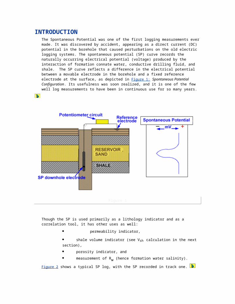
Figure 2

Rmf = (Rm)1.065 x 10((9 -W)/13)

Rmc = (Rm)0.88 x 10((W -10.4)/7.6)

where W is the mud weight in lb/gallon.

Another statistical approximation for predominantly NaCl muds is,

Rmf = 0.75 Rm

Rmc = 1.5 Rm

In all cases, direct measurement on a sample of mud filtrate is preferred. Even after determining values for SP, K, and Rmf, there are still minor problems to be solved. The equation,

SP = -K log (Rmf/Rw)

does not explain adequately the true electrochemical behavior of salt solutions. The actual SP development is controlled by the relative activity of the formation water and mud filtrate solutions. Thus the SP equation should read,

SP = -K Log (Aw/Amf)

where Aw and Amf are the activities of the connate water and the mud filtrate, respectively.

The resistivity of a solution is roughly proportional to the reciprocal of its activity at low salt concentrations, but at high concentrations there is a marked departure from this rule. A way to compensate for this departure is to define "effective" or "equivalent" resistivities for salt solutions that are, by definition, inversely proportional to the activities (Rwe = 0.075/Aw at 77 °F). A

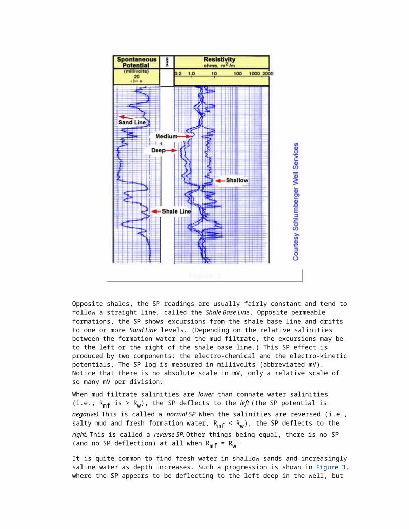
conversion chart is then used to go from an equivalent resistivity (Rwe) to an actual resistivity (Rw). The SP equation can then be rewritten to the strictly accurate formula,

SP = -K log (Rmfe/Rwe)

SHALE VOLUME CALCULATIONThe presence of shale in art otherwise "clean" sand tends to supress the SP. This effect can be used in estimating the shale content of a formation. If SPlog is the value of the SP curve at the desired measurement point on the log, and SPsand is the value observed in a clean, water-bearing sand and SPshale is the value observed in a shale, then any intermediate value of the SP may be converted into a value for the shale volume (Vsh) by the relationship

sandshale

sandSPsh SPSP

SPSPV

)()(

)()( log

This concept is illustrated in Figure   3: Shale Volume Calculation Example Using the SP.

Figure 3

GEOLOGICAL INFORMATION

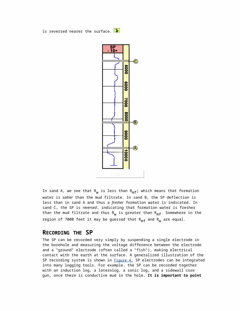
SP deflections often respond to changes in depositional environment. Characteristic SP shapes are produced in channels, bars, and other depositional sequences where sorting, grain size, or cementation changes with depth. These shapes are also called "bells" or "funnels." Figure   4: SP Shapes in Different Depositional Sequences illustrates some of these patterns.

Figure 4

FACTORS AFFECTING THE SPSP readings are usually accurately and easily measured. However, there are some circumstances where SP readings need careful consideration.

Oil-base muds completely lack an electrical path through the mud column, hence no SP can be generated.

Shaly formations suppresses the measured SP. This phenomenon permits the formation shaliness to be determined if a clean sand with the same water salinity is available for a legitimate comparison.

Hydrocarbon saturation suppresses SP deflections. Thus, only water-bearing sands should be selected for Rw determination from the SP.

Unbalanced mud columns, with differential pressure into the formation, can cause "streaming" potentials that augment the SP. This effect, known as electrokinetic SP, is noticeable in depleted reservoirs, and is impossible to compensate quantitatively.

Resistivities may be very high in hard formations, except in permeable zones or shales. These high resistivities affect the distribution of the SP currents, hence the shape of the SP curve. As illustrated in Figure   1: Schematic Representation of the SP in Highly Resistive Formations, the SP currents flowing from shale bed Shl toward permeable bed P2 are largely confined to the borehole between Shl and P2 because of the very high resistivity of the formation in this interval.

Figure 1

Accordingly, the intensity of the SP current in the borehole in this interval remains constant. Assuming the hole diameter is constant, the potential drop per foot is constant and the SP curve is a straight line.

In high resistivity formations, SP current can leave or enter the borehole only opposite permeable beds or shales. This causes the SP curve to show a succession of straight portions with a change of slope opposite every permeable interval (with the concave side of the SP curve toward the shale line) and opposite every shale bed (with the convex side of the SP curve toward the shale line). The boundaries of the permeable beds cannot be located with accuracy by use of the SP in such highly resistive formations.

Bed thickness can affect the SP measurement quite dramatically. In thin beds, the SP does not fully develop. Figure   2: Factors Affecting SP Reduction illustrates the factors which produce this effect.

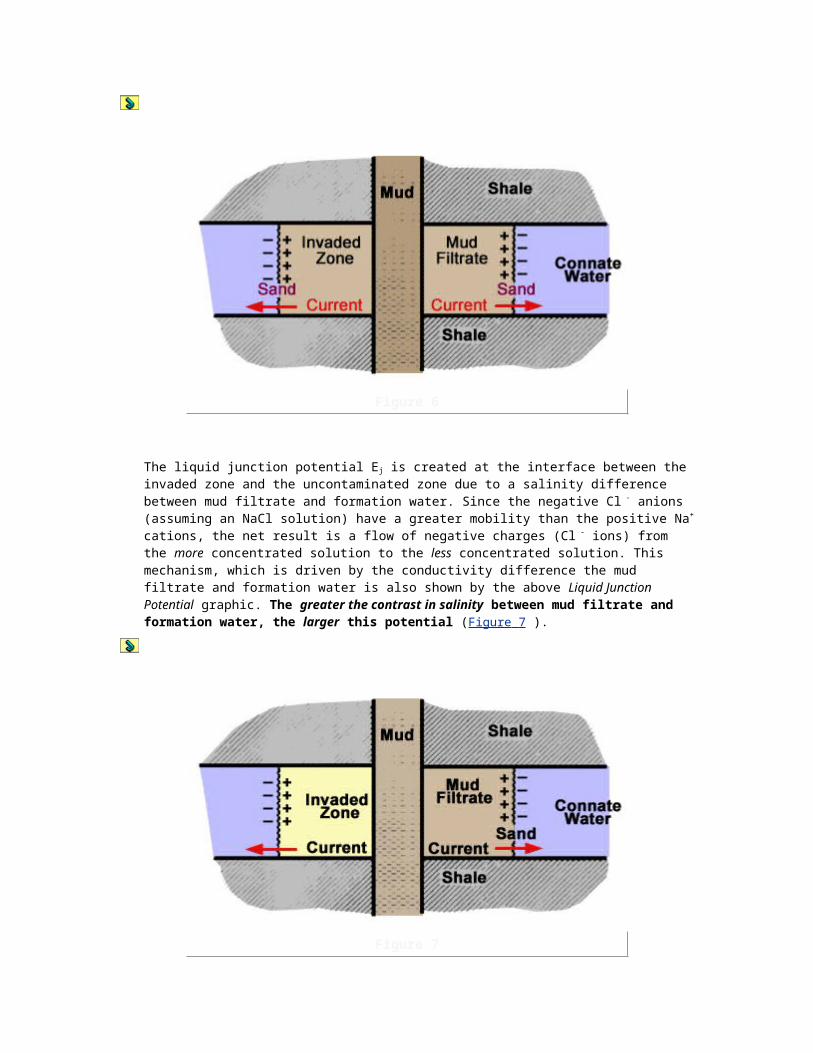
Figure 2

In the terminology used here, SP refers to the observed SP deflection on the log and SSP (static SP) to the value it would have if all disturbing influences been removed. Among the disturbing factors may be bed thickness, diameter of invasion, Rxo/Rm ratio, neighboring shale resistivity (Rsh), hole diameter (dh), and mud resistivity (Rm). In general, the SP reduction is greatest in thin beds, where Rxo/Rm is high and where invasion is deep.

Many SP correction charts are available in the literature, some more complex than others. It is virtually impossible for one chart to include all the variables involved in making necessary corrections. Figure   3: SP Correction for Bed Thickness shows a practicable chart, with most of the required variables (di, Rxo/Rm , and h) known or estimated.

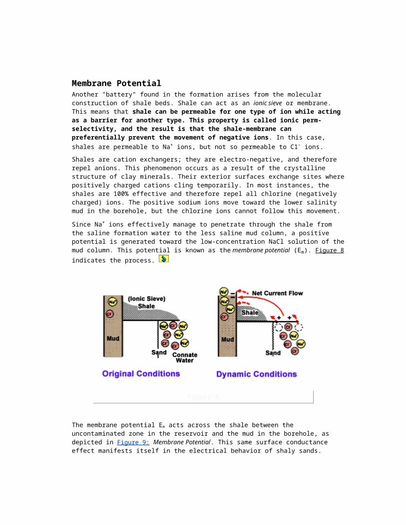
Figure 3

The use of non-NaCl muds (such as KCl) affects the derivation of Rw from the SP. Cox and Raymer (1976) cover this problem in detail. A quick solution to the KCl mud problem is to simply take the observed SP deflection, subtract 25 mV, and then treat it as a NaC1 mud case. The Rmf to Rmfe relationship is slightly different for KCl filtrates than for NaCl filtrates. Again, a quick rule of thumb is to add 30% to the measured Rmf and treat it as a NaCl filtrate.

Gamma Ray Log

 OVERVIEW Gamma ray logs are used for six main purposes:

Correlation between wells,

Determination of bed boundaries,

Evaluation of shale content within a formation,

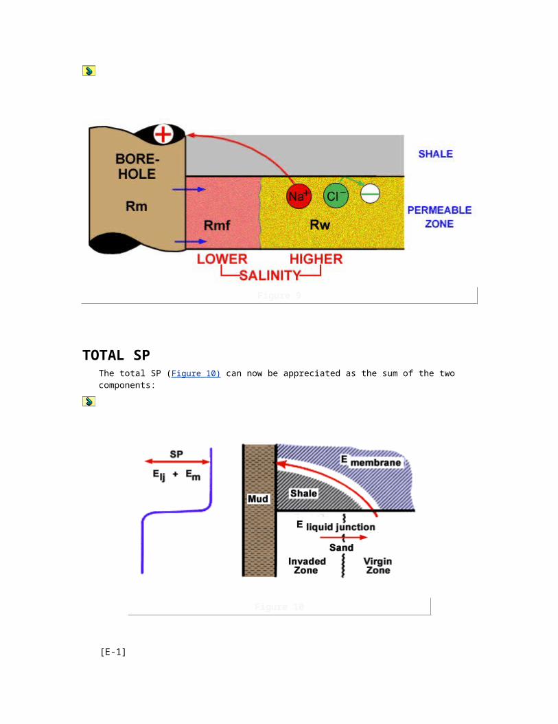
Mineral analysis,

Depth control for log tie-ins, side-wall coring, or perforating, and

Tracking movement of radioactive tracers

Gamma ray (GR) logs measure the natural gamma ray emissions from subsurface formations. Because gamma rays can pass through steel casing, measurements can be made in both open and cased holes. In applications not discussed here, such as pulsed neutron logging, induced gamma rays are measured.

Figure   1: Gamma Ray Log Example shows a typical GR log.

Figure 1

It is typically presented in track 1 on a linear grid and is scaled in API units. Gamma ray activity increases from left to right. Gamma ray tools consist of a detector and the associated electronics for passing the gamma ray count rate to the surface. These tools are in the form of double-ended subs that can be sandwiched into practically any logging tool string; thus, the GR log can be run with practically any tool available.

Gamma rays originate from three main sources in nature: the radioactive elements in the uranium and thorium groups, and potassium. Uranium 235, uranium 238, and thorium 232 all decay, via a long chain of daughter products, to stable lead isotopes. An isotope of potassium, K40, decays to argon.

An "average" shale contains 6 ppm uranium, 12 ppm thorium, and 2% potassium. Since the various gamma ray sources are not all equally effective, it is more informative to consider potassium equivalents (i.e., the amount of potassium that would produce the same number of

gamma rays per unit of time). Reduced to a common denominator, the average shale contains uranium equivalent to 4.3% potassium, thorium equivalent to 3.5% potassium, and 2% potassium.

An average shale is hard to find. Since a shale is a mixture of clay minerals, sand, silts, and other extraneous materials, there can be no standard gamma ray activity for shale. Indeed, the main clay minerals vary enormously in their natural radioactivity. Kaolinite and chlorite have no potassium, whereas illite contains between 4% and 8% potassium. Montmorillonite contains less than 1% potassium. Occasionally, natural radioactivity may be due to the presence of dissolved potassium or other salts in the water contained in the pores of the shale.

Each radioactive decay produces a gamma ray that is unique. These various gamma rays have characteristic energy levels and occur in characteristic abundance, as expressed in counts per time period. Counting how many gamma rays a formation produces can be carried a step further to counting how many from each gamma ray energy group it produces. If the number of occurrences is plotted against the energy group, a spectrum will be produced that is characteristic of the formation logged. The relationship between gamma ray energy and frequency of occurrence, shown in Figure   2: Gamma Ray Spectrometry shows such a spectrum, where energies from 0 to approximately 3 Mev have been split into 256 specific energy "bins." The number of gamma rays in each bin is plotted on the Y-axis.

Figure 2

This spectrum can be thought of as a mixture of the three individual spectra belonging to uranium, thorium, and potassium. Some unique mixture of these three radioactive "families" would have the same spectrum as the observed one. The trick is to find a quick and easy method of discovering that unique mixture. Fortunately, on-board computers in logging trucks are capable of quickly finding a "best fit" and producing continuous curves showing the concentration of U, Th, and K.

In a gamma ray spectral log, note that in track 1 both total gamma ray activity (SGR) and a "uranium-free" (CGR) version of the total activity are displayed. Units are API. In tracks 2 and 3, the concentration of U, Th, and K are displayed. Depending on the logging service company the units may be in counts/sec, ppm, or %.

GAMMA RAYS & NATURAL RADIATIONNuclear logging instruments can be divided into a passive group that only contain radiation detectors, and an active group that contain both a radioactive source and detectors. These two types of tools measure:

Natural Radioactivity - usually by means of recording the gamma-rays that are emitted by elements in the formation, and

Induced Radioactivity -which requires a radioactive source to emit neutrons or gamma-rays that penetrate the borehole and the surrounding formation. The gamma-ray density and neutron porosity tools that use such radioactive sources will be discussed in different subject areas.

In this section, we will deal exclusively with natural radioactivity.

NATURAL RADIOACTIVE ELEMENTSRadioactivity is associated with the structure of chemical elements. An element contains protons and neutrons in its nucleus, along with electrons in one or more orbits. Each element is identified by its unique number of protons (Z-number). The majority of elements consist of a mixture of two or more isotopes.

Isotopes have the same number of protons, but a different number of neutrons. Many isotopes are unstable and emit alpha, beta and/or gamma radiation, to permute to a stable isotope. Of these three types of radiation, only the gamma-rays can be recorded with logging tools in the well, because beta and alpha particles have a very limited penetration depth -often less than one cm in heavy materials. Gamma-rays (photons) have a considerable penetration depth and thus allow recording of natural gamma-radiation emitted by rocks through steel casing. This means that natural gamma ray logs are often run in both cased and open holes.

ORIGIN OF NATURAL GAMMA RADIATIONThe gamma rays encountered in the borehole can be chiefly attributed to 3 main sources in nature: the radioactive elements in the uranium group, the thorium group, and potassium.

U-Ra

 

: uranium-radium elements and their unstable daughter series of elements

 Th

 

: thorium series

 K40

 

: potassium-40 isotope

 Uranium 235, uranium 238, and thorium 232 all decay to stable lead isotopes, via a long chain of daughter products. An isotope of potassium, K40, decays to argon, and gives off a gamma ray in the process.

It should be noted that each type of decay is characterized by a gamma ray of a specific energy (wavelength), and the frequency of occurrence for each decay energy is different. Potassium-40 emits gamma-rays with one single radiation energy (1.46 MeV), whereas the U-Ra and Th series display a wide range of energies. The radiation intensity (photons per gram per second) is:

2600 for U-RA

12000 for Th

3 for K40

Figure   1 shows this relationship between gamma ray energy and frequency of occurrence. This is an important concept, since it is used as the basis for measurement in the natural gamma spectroscopy tools.

Figure 1

Radioactivity in Shales

The basic constituents of igneous rocks are:

quartz, with a low degree of radioactivity

feldspars and mica's, with K40 and sometimes U-Ra and Th

Feldspars decompose at a relatively rapid rate into clay minerals, and radioactive-elements are trapped in their rock fabric. Because clay minerals are the principle constituents of shales, these are generally radioactive as well.

An "average" shale contains 6 ppm uranium, 12 ppm thorium, and 2% potassium. Since the various gamma ray sources are not all equally effective, it is more informative to consider this mix of radioactive materials on a common basis, e.g., by reference to potassium equivalents (i.e., the amount of potassium that produces the same number of gamma rays per unit of time). Reduced to a common denominator, the average shale contains 2% potassium along with uranium equivalent to 4.3% potassium, and thorium equivalent to 3.5% potassium.

Average shales are hard to find. Shale, being a mixture of clay minerals, sand, silts, and other extraneous materials, exhibits no "standard" gamma ray activity. Indeed, the main clay minerals vary enormously in their natural radioactivity: kaolinite has no potassium, illite has between 4% and 8% potassium, while montmorillonite less than 1%. Occasionally, natural radioactivity may be due to the presence of dissolved potassium or other salts in shale pore water. Additionally, shale is not necessarily the strongest gamma-ray emitting lithology in a reservoir. Very good reservoir sands found in some parts of the North Sea contain mica, which holds a significant amount of radioactive potassium. This situation can lead to gamma-radiation levels in clean sands that are as high as levels in the surrounding shales.

GAMMA-RAY DETECTORSThe first measuring instruments used Geiger-Müller tubes to detect gamma-rays. These tubes have the disadvantages that the count-rates are low and the output is not proportional to the energy of the individually detected gamma photons. Since the 1960’s, scintillation counters have been used to measure radioactivity in boreholes. These counters are based on the physical phenomenon that when gamma-rays interact with the lattice of the scintillation crystal, visible light flashes are produced. The most widely used crystal material has been the Thallium-activated sodium iodide NaI, but other materials such a BGO (Bithmuth-germanium-oxide) and GSO (Gadolinium oxy-ortho-silicate) gain in popularity due to their higher density, and therefore more efficient conversion of gamma-rays to scintillations. Figure   2 (Scintillation detector) shows an example of an NaI detector. The one main exception is within the MWD industry. Many MWD natural gamma-ray tools still rely on several banks of Geiger-Muller tubes working together in order to accomplish their task.

Figure 2

OPERATING PRINCIPLE OF GAMMA RAY TOOLSWhen a gamma ray strikes the crystal, a single photon of light is emitted. This tiny flash of light then strikes a photo-cathode made from cesium-antimony or silver-magnesium. When the light quanta hit the photo-cathode of a photo-multiplier, they dislodge one or more electrons. These electrons are in turn accelerated by a cascade circuit of electrodes, where each subsequent

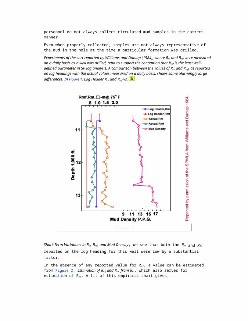
electrode has a higher voltage, and more electrons are dislodged at each stage. This multiplication process leads to an avalanche of electrons that produce a measurable electric pulse at the last anode of the tube. An attractive feature of this technique is that the pulse height is proportional to the energy of the original gamma-photon allowing the detector to be used as a gamma-ray spectroscopy device. The system has a very short "dead time" and can register many counts per second without becoming swamped by numerous signals.

CALIBRATION OF GAMMA RAY DETECTORS AND LOGSOne problem of gamma ray logging is choosing a standard calibration system. This is because all logging companies use a variety of counters encased in different steel housings of various sizes and shapes. On very old logs, the scale might be quoted in micrograms of radium equivalents/ton of formation. For many reasons, this method was found to be unsatisfactory to calibrate gamma ray logs, so an API standard was devised. A test pit (installed at the university of Houston) contains an "artificial shale"(

Figure   1: API Gamma Ray Standard).

Figure 1

A cylinder 24 ft long and 4 ft in diameter contains a central 8-ft section consisting of cement mixed with 13-ppm uranium, 24-ppm thorium, and 4% potassium. On either side, completing the sandwich, are 8-ft sections of neat Portland cement cased with 5-1/2 inch J55 casing. The API standard defines the difference in radioactivity between the neat cement and the radioactively doped cement as 200 API units. Any logging service company may place its tool in this pit to make a calibration.

Field calibration is performed using a portable jig that contains a radioactive "pill." Placed over the center of the gamma ray detector, the jig produces an increase over the background count rate equivalent to a known number of API units, depending on the tool type and size and the counter it encloses.

TIME CONSTANTS

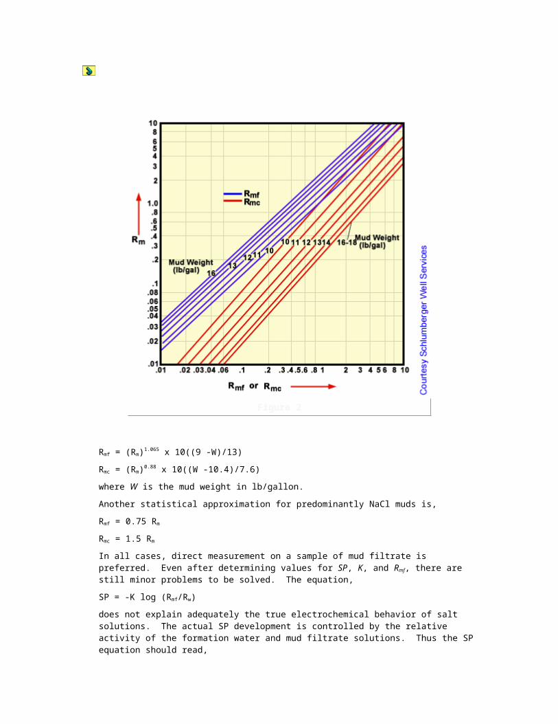
Radioactive emissions are random phenomena that are subject to statistical variations. Since they vary in time, they produce statistical fluctuations on the gamma-ray log. For example, if a radioactive source emits an average of 360,000 gamma rays per hour over a period of hours, then we can suppose that the source will emit 100 gamma rays per second (100/sec. x 60 seconds x 60 minutes). If the count is measured for 1 second, however, the actual count might be more or less than 100, thus forcing a choice. A relatively quick gamma ray count provides a poor estimate of the real count rate, while a long count yields a more accurate estimate of the count rate at the expense of much rig time.

The logger must therefore choose between various time constants, according to the radioactivity level measured. The lower the count rate, the longer the time constant required for adequate averaging of variations. In the past, a simple resistor -capacitor (R-C) circuit was used; however, nowadays the averaging is carried out digitally after an analog to digital (A-D) conversion. The time-averaging constant (TC) helps to smooth the gamma-log. The faster the tool moves through the hole, the fewer gamma rays will be counted per depth unit, so a longer time averaging period has to be employed to smooth out the statistical fluctuations.

On a typical logging job, gamma rays might be counted for a short period of time (e.g., one second); however, we must remember that during this 1-second time frame, the gamma ray detector will have moved past the formation whose activity is being measured. Thus, the logging speed and the time interval used to average count rates are interrelated. The following rules of thumb are generally recognized.

Table 1: Logging Speeds

Logging Speed

 

Time Constant

 3600 ft/hr

 

1 sec

 1800 ft/hr

 

2 sec

 1200 ft/hr

 

3 sec

 900 ft/hr

 

4 sec

 A theoretical example is given in Figure   2: Example of Boundary Displacement GR Reading.

Figure 2

For a logging speed of 1800 ft/hr and a time-averaging constant TC = 2 sec, the time lag produces an apparent boundary displacement of about 1 foot. The averaging procedure causes a time lag on the log boundaries which increases with logging speed and TC, as demonstrated in the table embedded in the above graphic. The selection of the TC is a practical compromise of logging speed and log quality, as shown in the table below. The standard for most logging jobs is 1800 ft/hr and a TC of 2 sec.

Table 2: Logging Speed versus Log Quality for the GR Measurement

Logging speed (ft/hr)

 

3600

 

1800

 

1800

 

900

 Time constant, (sec)

 

5

 

5

 

2

 

4

 Statistical variations

 

low

 

low

 

fair

 

low

 Travel during TC, ft

 

5

 

2.5

 

1

 

1

 Thin bed definition

 

poor

 

poor

 

good

 

good

 The parameters listed in the last column of this table can be used over short intervals for good bed definition. It is customary to maintain the product of logging speed (ft/sec) and TC (sec) at one foot.

The investigation volume of the Gamma Ray tool has the shape of a sphere around the detector. The depth of investigation is determined by:

Rock density, and mud density that attenuate the gamma-rays

Natural GR energy

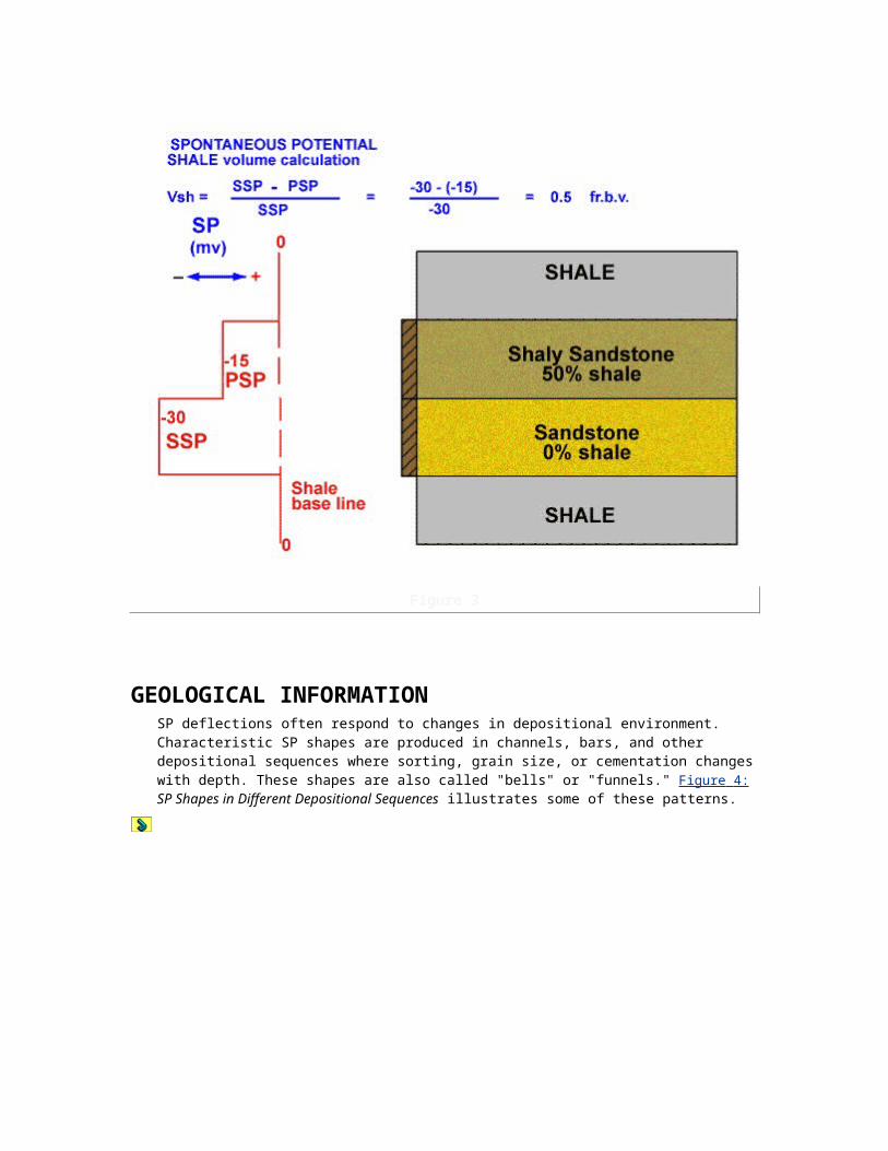
Detector length (4'', 8'', and occasionally 12")

A rough value for the vertical resolution is 2 feet, while the depth of investigation is about 1 foot.

In the future, when the efficiency of gamma ray detectors and their associated electronics improves by one or two orders of magnitude, the use of a time constant will be obsolete except in the cases of extremely inactive formations with intrinsically low gamma ray count rates.

PERTURBING AFFECTS ON GAMMA RAY LOGSGamma ray logs are subject to a number of perturbing effects, including

Sonde position in the hole (centered/eccentered)

Hole size

Mud weight

Casing size and weight

Cement thickness

Since there are innumerable combinations of these effects, an arbitrary standard set of conditions is defined as a 3-5/8 in. OD tool, eccentered in an 8-in. hole filled with 10-lb mud. A series of charts exists for making the appropriate corrections. Note that if a gamma ray log is run in combination with a neutron density tool, it is run eccentrically. If run with a laterolog or an induction log, it is usually centered.

GAMMA RAY SPECTROSCOPYEach radioactive decay produces a gamma ray that is unique in terms of energy level and abundance, and which is expressed in counts per time period. The simple method of counting how many gamma rays a formation produces can be carried a step further to count how many gamma rays from each energy group it produces. If the number of occurrences is plotted against the energy group, a spectrum can be produced that is characteristic of the formation logged.

Figure   3 shows such a spectrum, where energies from 0 to approximately 3 MeV have been split into 256 specific energy "bins." The number of gamma rays in each bin is plotted on the Y-axis.

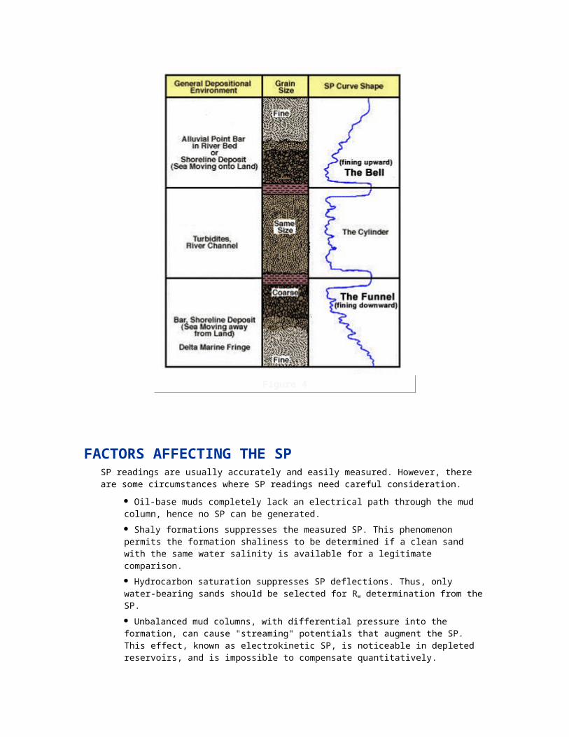
Figure 3

This spectrum can be thought of as a mixture of the three individual spectra belonging to uranium, thorium, and potassium. A unique mixture of these three radioactive "families" has the same spectrum as the one observed. The trick is to find a quick and easy method of discovering that unique mixture. Fortunately, the on-board computers in logging trucks are capable of quickly finding a "best fit" to produce continuous curves showing the concentration of U, Th, and K.

Figure   4 illustrates a gamma ray spectral log.

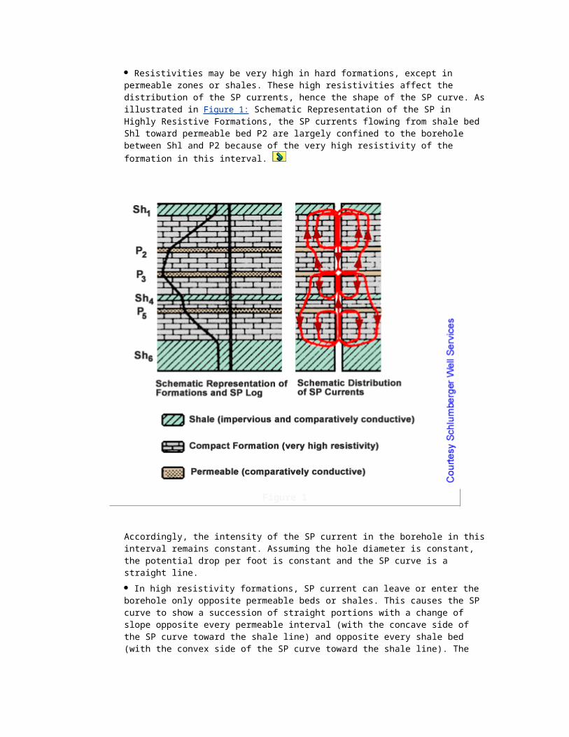
Figure 4

Note that in Track I, both total gamma ray activity (SGR) and a "uranium free" version of the total activity are displayed (units are API). In Tracks II and III the concentrations of U, Th, and K are displayed. Depending on the logging service company, the units may be in counts/sec, ppm, or percentage.

Resistivity Logs

INTRODUCTIONThe first logging device ever designed measured formation resistivity. It was a modification of a method previously used to detect underground resistivity anomalies associated with either geologic features or concentrations of metallic ores. Figure   1 illustrates this old surface surveying method.

Figure 1

A voltage source sent a current through the ground between two widely spaced electrodes. The voltage drop between two other more closely spaced electrodes was used as a measure of the ground resistivity. By moving the whole electrode array across the countryside, it was possible to "map" underground features, as shown in Figure   2.

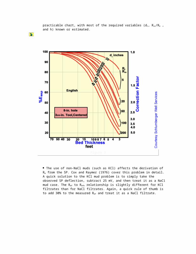
Figure 2.

By rotating the whole setup by 90° and lowering it into a borehole, the electric log was born.

There is now a bewildering variety in the design and principles used for resistivity logging. While we usually only want to know true resistivity (Rt), over a dozen resistivity tools have been developed in an effort to acquire this measurement. The reason for this abundance of designs is that resistivity of the borehole, the mud filtrate, and adjacent beds all have an effect on the resistivity measured by a tool in the borehole. No single design can fully compensate for all these effects, and a combination of measurements with different tools is required to calculate the illusive Rt

Since the early days of wireline well logging, a series of improvements have resulted in five main families of resistivity tools. These include:

electric logs,

induction logs,

laterologs,

microresistivity devices, and

dielectric logs

Additionally, Measurement While Drilling (MWD) technology has been quick to develop tools that perform the same tasks as their wireline counterparts.

EVOLUTION OF RESISTIVITY LOGS

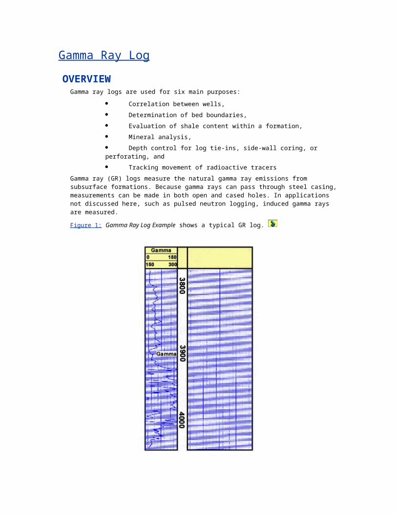
Although the original electric logging principles were sound, their practical implementation left much to be desired. Efforts to improve the measurement of formation resistivity have been continually pursued since the inception of the electric log. As a result, several classifications of resistivity logging have evolved: the electrical survey (ES), Laterologs, Induction Logs, Micro-Resistivity Logs, and Dielectric Logs (also known as electromagnetic propagation tools).

ELECTRIC SONDEThe first resistivity log, an electrical survey, was run in 1927 by Marcel and Conrad Schlumberger in the Pechelbronn Field of France. It was downhole adaptation of the Pole-Dipole surface resistivity method used in mineral exploration. This ES tool contained 3 lead electrodes held together with ropes. One electrode, which was grounded to the surface, was used to inject current via the borehole into the formation. The other two electrodes measured the potentials generated by this injected current.

The measured voltages provided the resistivity determinations for each device, as follows: In Figure   3,

Figure 3

a current I flows between electrode A and electrode N in a homogeneous, isotropic medium. The corresponding equipotential surfaces surrounding the current emitting electrode A would be spherical. The voltage on electrode N situated on one of these spheres is proportional to the resistivity of the formation, and the measured voltage can be scaled in resistivity units.

The ES was able to detect layer boundaries and high resistivities (typically indicative of oil). Using the ES, formation resistivity values could only be obtained when used in slim boreholes having relatively high mud resistivity, shallow invasion, and thick beds. Although the original electric logging principles were sound, their practical embodiments left much to be desired. Efforts to improve the measurement of formation resistivity have been busily pursued for several decades. As a result, three main branches of resistivity logging have evolved: induction logs, focused electric logs, (in both induction and laterolog varieties) and microwave devices.

The first overseas ES log was run in Brunei (Borneo) in 1929. ES logs, although rarely used today in western oil and gas logging operations, are still discussed because a large proportion of well data from older fields consists solely of ES logs.

INDUCTION LOGSBefore the Second World War, many wells were drilled with muds that consisted of locally available clay and water mixtures of low salinity. These muds were often incompatible with the shales encountered downhole, which led to clay swelling, large wash-outs, and even caving of wells. In the early 1950's, oil-base muds were developed with diesel fuel as the continuous phase, and therefore significantly reduced clay problems. However these muds did not conduct electric currents, so ES tools with electrodes could not be applied anymore.

Induction tools were developed for these circumstances. Rather than using current and voltage electrodes, the induction log introduced a system of focused coils that induce the flow of currents in the formation away from the disturbing influence of the borehole and the invaded zone. Experience soon demonstrated that the induction log had many advantages over the conventional ES log when used in wells drilled with water-based muds. Designed for deep investigation, induction logs can be focused to minimize the influences of the borehole, the surrounding formations, and the invaded zone. Spherically focused induction logs provide deep, medium, and shallow readings.

These tools can also be used in air-drilled holes to derive conductivity values of the formation using electromagnetic coupling of transmitter and receiving coils in the logging tool via the conductive rock surrounding non-conductive borehole.

LATEROLOGSLaterolog tools were developed for high salinity drilling muds, applied to drill through salt layers, in which ES tools are virtually short-circuited. The laterologs use arrays of electrodes to focus the current emitted by the center electrode into the formation, and thereby significantly reduce the effect of the mud. Both the induction and laterolog tools are superior to the older ES tools to obtain a reliable value of the true resistivity of the uninvaded formation. These tools are much superior to the conventional electrical logs (ES) because they eliminate many of the detrimental borehole effects. They are also provide better resolution of thin beds. Focusing electrode systems are available with deep and medium depths of investigation, and are often run in tandem with a micro-resistivity log to provide a very shallow reading.

MICRO RESISTIVITY TOOLSMicro resistivity tools were introduced to provide an accurate assessment of the resistivity of the mudcake (Rmc) and the invaded zone Rxo. These tools have very close electrode spacing, with electrodes mounted on a pad that is pushed against the borehole wall to minimize the effect of the borehole fluid.

HIGH-RESOLUTION INDUCTION TOOLSFrom the 1960s to the mid-1980s, the Dual Induction logging tool provided the primary logging service for openhole formation evaluation in fresh-water and oil-base muds. However, certain design limitations caused problems with the induction response, resulting in formation resistivity measurements that were distorted by adjacent beds, the invaded zone, and even by the borehole. The most serious of these were

Resistivity readings that caused estimates of formation water resistivity (Rw) to be much lower than those indicated by spontaneous potential or by measurements of recovered water samples.

Separation between the deep, medium, and shallow focused responses in tight, high-resistivity formations where other measurements indicated little or no invasion.

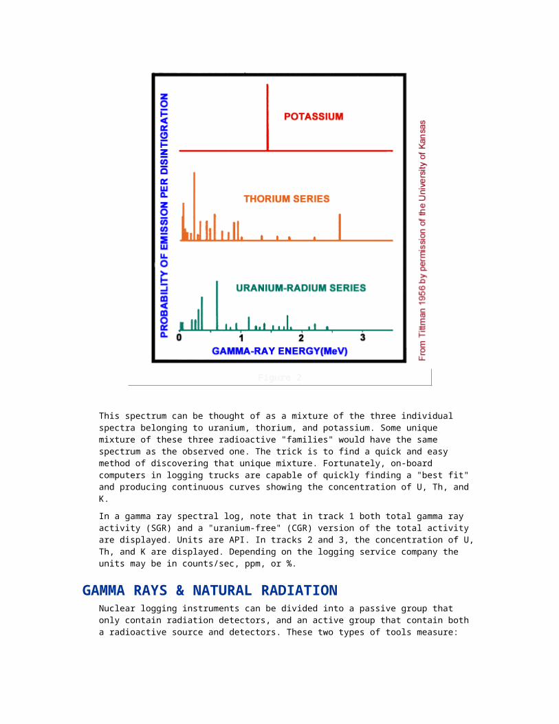
Poor vertical resolution of 8 feet for the deep induction measurements and 6 feet for the medium curve.

Distortions stemming from resolution and shoulder effect had been predicted through electromagnetic theory; however, automatic correction algorithms were unsuccessful, owing to the non-linearity of the R-signal measurement, which was the only measurement made by the dual induction tools. These limitations in tool response were recognized by logging companies and their clients, but the tool represented the best technology of the time.

During the mid-1980s, advances in electronics technology and signal processing led to improved output from standard dual induction hardware. Improvements arose from the use of both the conventional (indirect) EMF’s induced in the receiver coil and the directly coupled, out of phase, "X signals." These newer induction tools are referred to as high-resolution induction (HRI) or phasor induction tools. Central to the development of the Phasor tool was a nonlinear deconvolution technique that corrects the induction log in real time for shoulder effect and improves the thin-bed resolution down to 2 ft in many cases. This algorithm uses the induction quadrature signal, or X-signal, which measures the non-linearity directly.

The result of the additional data is a measurement of formation resistivity which is less affected by adjacent beds and allows far better precision in correcting for invasion effects. Modern software routines allow real-time deconvolution in the logging unit and hence output of Rt, along with Rxo

and diameter of invasion (di) directly onto the log.

Figure   4 : Induction Log Comparison shows the same formation logged with (a) a conventional dual induction and (b) an HRI log. Note the improvement in bed resolution between (a) and (b).

Figure 4

ARRAY INDUCTION TOOLThough the high resolution induction tool was an improvement over the dual induction tool, there was still a need for a tool capable of providing better estimates of Rt in the presence of deep invasion or complex transition zones.

One approach would be to recombine multiple arrays to produce a set of measurements at several depths of investigation and then invert the measurements radially to obtain an estimate of Rt. The concept of multiple measurements was put forth as early as 1957 by Pupon, but at the time, technical limitations on the amount of data that could be transmitted to the surface via logging cable hindered early development of such an array tool.

Modern array induction tools are constructed of eight independent arrays with main coil spacings ranging from 6 inches to 6 feet. Each array consists of a single transmitter coil and two receivers. All measurements are simultaneously acquired every 3 inches of depth.

Log processing makes full environmental corrections and the logs are virtually free of cave effect and can be used to provide an accurate Rt estimate and a quantitative description of the transition zone in both oil-and water-base mud systems.

The processing algorithm for array induction tools works as well when Rxo < Rt and when

Rxo > Rt -within limits. The chief limitation of array induction tools in salty muds is their ability to make accurate borehole corrections. In cases where the mud is salty and the borehole is rugose, the traditional laterolog tool would be the resistivity tool of choice. For most applications where Rt/Rm> 500, the laterolog provides a closer estimate of Rt; however, the array induction tools contribute important invasion information even in these cases. For salty mud, a combination of array induction and laterolog tools would produce a better total answer than either tool alone.

3D INDUCTION TOOLIt has been estimated that 30% of the world’s oil reserves will be found within thinly laminated formations. However, thin-bedded laminated formations pose a special problem for log analysts. The thin shale layers in these formations do not alter the porosity and permeability characteristics of the inter-bedded sands, but the highly conductive nature of the shales greatly suppresses standard induction log response. The term "low-contrast pay" is often applied to such intervals of inter-bedded sands and shales, which typically exhibit a combined resistivity of only a few tenths of an Ohm-m over adjacent shales.

Experience has shown that these formations are often capable of producing at very high rates. Identifying and quantifying hydrocarbon reserves in low resistivity formations can have major economic impact on such a prospect.

Low resistivity pay can be attributed to two different modes. It can be found in thinly bedded laminated sand-shale formations. Or it can be found in sand layers of varying grain size distributions that create an electrical anisotropy caused by variations in water saturation and fluid morphology. These potentially productive intervals are almost indistinguishable from adjacent shales, given the poor vertical resolution of conventional resistivity tools. Such measurements will only be satisfactory when evaluating formations that are at least as thick as the tool’s vertical resolution.

Conventional induction logging tools are limited to measurements in one dimension because their sensors are aligned along the tool or Z-axis. These tools measure horizontal resistivity, which is measured parallel to the bed. Horizontal resistivity is dominated by the low resistivity of the shale laminae, rather than by the higher resistivity of the hydrocarbon-bearing sand laminae. Conventional tools will not adequately resolve the electrical anisotropy of low resistivity formations.

Baker Atlas offers a 3D induction tool designed to identify and quantify hydrocarbons in laminated, low-resistivity pay formations. The Baker Atlas 3D Explorer service characterizes formation

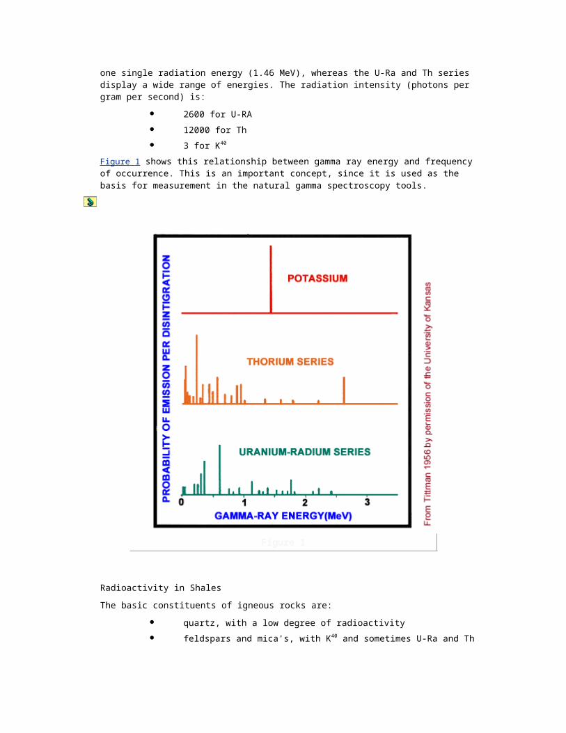
resistivity in three dimensions. Like conventional tools, this logging tool employs sets of "Z" direction coils that are aligned coaxially with the instrument; but unlike conventional tools, it also carries orthogonally mounted "X" and "Y" coil arrays. This configuration, together with specially developed software, provides the information necessary to determine vertical resistivity (Rv) and

horizontal resistivity (Rh) from the 3D induction data. Vertical resistivity is sensitive to the hydrocarbon-bearing laminated sand within sand-shale sequences.

When Rv is greater than Rh the formation is said to exhibit electrical anisotropy. The ratio of Rv/Rh determines the value of the electrical anisotropy ratio. The vertical resistivity and the anisotropy ratio are sensitive to changes in both laminar shale content and to laminar sand resistivity.

On the log presentation, the separation between horizontal and vertical resistivity curves is used to identify zones of transverse anisotropy. Transverse anisotropy associated with the laminated formation structure is used to flag the presence of hydrocarbons within the sand laminae.

DIELECTRIC TOOLSMicrowave devices (also called electromagnetic propagation logging) were built to measure the dielectric constant and conductivity of the formation. Strictly speaking, they do not measure formation resistivity; however, they are often classified as resistivity devices since their end use is the same as for resistivity devices, i.e., determination of formation fluid saturation.

RESISTIVITY LOGS FOR BOREHOLE IMAGINGReservoirs characterized by thin beds or fractures are prime candidates for the detailed evaluation provided by borehole imaging tools. These tools offer vertical resolution finer than 1 foot, and produce images of the formation that are colored according to formation conductivity. These images can show changes in fluid properties, permeability, porosity, rock composition, and grain texture.

Resistivity imaging tools are offered by the major logging companies, who provide the following products:

Baker Atlas: Simultaneous Acoustic / Resistivity (STAR) Tool

Halliburton: Electrical MicroImaging (EMI) Tool

Schlumberger: Formation MicroImager (FMI) Tool, andAzimuthal Resistivity Imager (ARI)

These tools are further discussed in the presentation on Resistivity Imaging, found under the subtopic entitled Borehole Imaging Technology.

CASED HOLE RESISTIVITY LOGSCased hole resistivity logs offer deep-reading resistivity measurements to aid in locating bypassed pay behind pipe, for reservoir monitoring, or contingency logging. These tools will be further discussed in the Petroleum Engineering presentation on Cased Hole Resistivity Logs, found under the subtopic entitled Formation Evaluation in Cased Holes.

TOOL RESPONSEWhatever device is used to measure formation resistivity, a number of common factors conspire to confound these efforts, such as:

Effects of the borehole

Effects of neighboring beds

Effects of mud filtrate invasion.

Although modern resistivity-measuring devices represent a considerable improvement over the original unfocused electric log (commonly called the old E-log), there is still plenty of room for improvement. In addition to Rt, the resistivity of the undisturbed zone (which is what we are trying to measure), the tool, by its design, can be influenced by the resistivities of the mud in the borehole, the adjacent beds, and the mud filtrate in the invaded zone (Figure   1: Simplified model

of a borehole profile).

Figure 1

Thus, we cannot always assume that the reading from a resistivity log truly represents Rt.

When reading a resistivity log, the log analyst should remember that the measurement is a composite of the four items in Figure   2: Factors affecting resistivity devices.

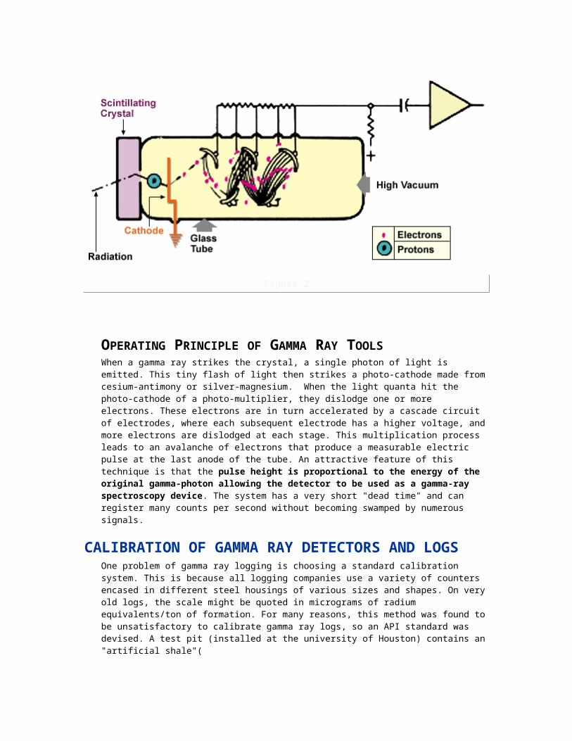
Figure 2

Depending on the device used, the particular conditions in the well, and the formations logged, the actual reading may be greater or less than Rt.

Later, we will discuss how to recognize cases where resistivity measurements depart radically from Rt. For now, remember that, as a rule, a large contrast between the resistivity of the bed of interest and the resistivity of either the mud column or the adjacent bed is a danger signal that calls for the use of correction charts. In this context, a "large" contrast could be classified as a factor of 10 or more. Of particular note are conditions where the bed of interest is thin (say, 15 feet or less) and/or invasion is deep (di greater than 40 inches).

To summarize, assume that a deep-resistivity device measures Rt unless:

Rt /Rm is greater than 10

Rt /Rs is greater than 10

Hole size is greater than 12 inches

The bed is thinner than 15 feet

Invasion is greater than 40 inches

If any of these adverse conditions exists, refer to the appropriate correction chart. As will become apparent, induction logs and focused electric logs (laterologs) behave differently when faced with these problems; in many cases, the same conditions that adversely affect an induction tool will be advantageous to a laterolog, and vice versa.

CONVENTIONAL ELECTRIC LOGSThe basic electric resistivity logging system consists of two current electrodes A and B (the ground return) and two voltage measuring electrodes M and N. These can be arranged in a variety of configurations and spacings to suit particular survey requirements, such as bed resolution or depth of investigation. Some of these arrangements have become industry standards, such as the Normal and the Lateral electrode spacings.

        < Normal Devices

Figure 1: Normal Resistivity Device, illustrates the electrode arrangement for the Normal tool.

Figure 1

Constant current is passed between electrodes A and B. The voltage potential is measured between electrodes M and N. The distance AM is called the electrode spacing. Thus, the 16-inches. short-normal device has electrode A separated from electrode M by 16 inches. The normal device is a downhole adaptation of the pole-pole geometry used in surface geophysical resistivity methods.

        LATERAL DEVICESFigure   2: Lateral Resistivity Device illustrates the arrangement for a Lateral tool.

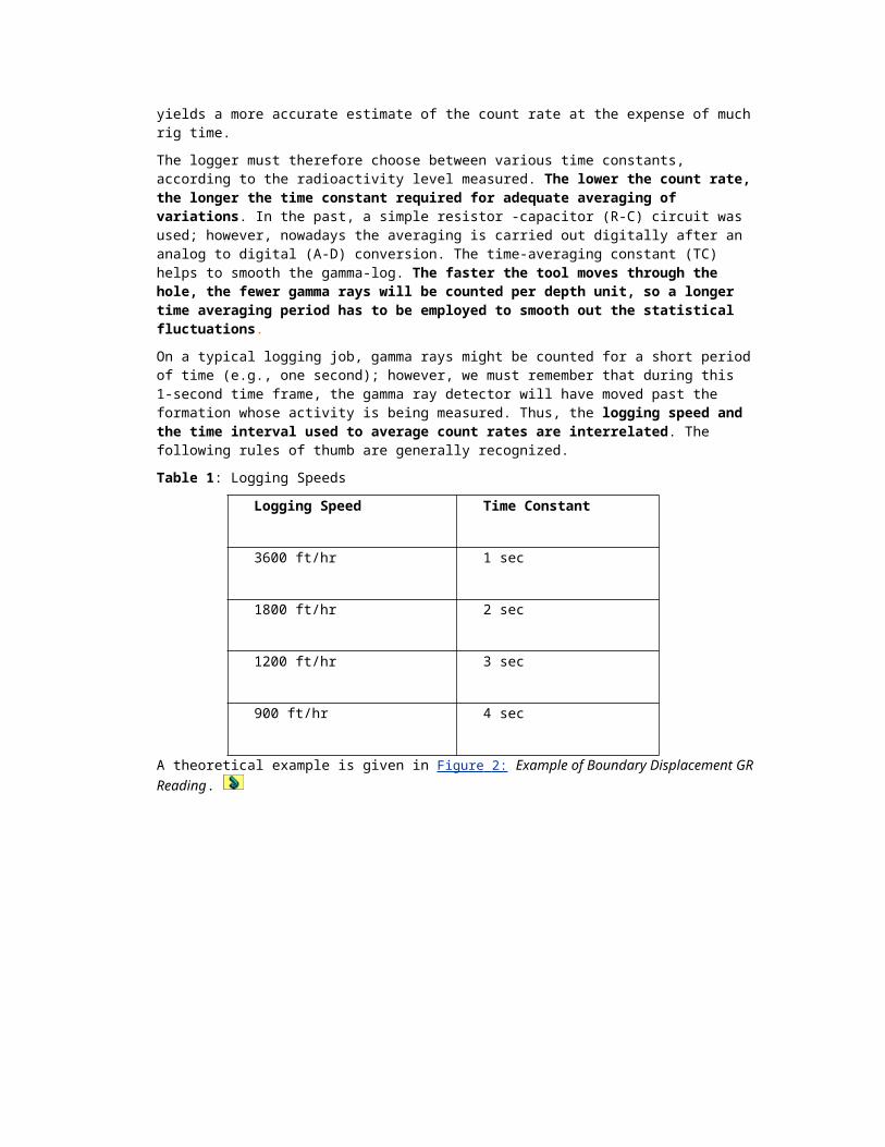
Figure 2

A constant current is sent between the A and B electrodes while the voltage potential is measured between the M and N electrodes. The lateral device is a downhole adaptation of the pole-dipole geometry used in surface geophysical resistivity methods.

SHORT NORMAL (SN), LONG NORMAL (LN), AND LATERAL TOOL DESCRIPTIONSWith wireline logging tools, the very presence of a borehole severely hampers the determination of the true formation resistivity. This is due to the conductivity (or lack of conductivity for oil base muds) of the borehole itself. If we could place electrodes in the ground without drilling (an exercise in imagination), we could pass an electric current between electrode "A" embedded in an infinite, homogenous isotropic medium and electrode "B" at an infinite distance. The current would then flow radially outward in all directions as illustrated in Figure   3: Potential Distribution in the Radial Flow of Electricity. In this case, the equal-potential surfaces are spherical, with their centers at the current electrode "A".

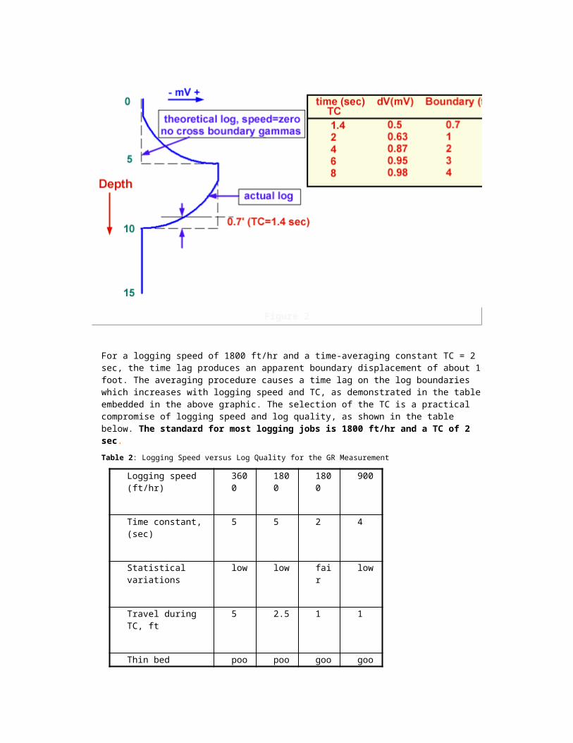
Figure 3

If we place another electrode "M" near "A", then electrode "M" will lie on the sphere whose radius is the distance AM. If "M" is connected through a potentiometer to a remote electrode "N", then this meter will indicate the potential at the sphere of radius AM.

For a sphere, the potential difference between electrode M and electrode N is:

[E-1]

  AM4

RIdL

L4

RIEE

AN

AM2nm

 This can be rearranged as:

[E-2]  I

EKR n

 where Kn is a proportionality factor depending on the electrode spacings. If the tool emits a constant current I and the potential difference E is measured, R can then be calculated.

Electrodes in the borehole measure the potentials Em and En. If the borehole resistivity does not deviate too much from the formation resistivity, these potentials correspond to similar potentials in the rock formation, as shown in Figure   4: Current Distribution With and Without a Borehole / Layer

Disturbance.

Figure 4

The greater the distance of the two measuring electrodes from the current electrode A, the deeper these equal-potential spheres reach into the formation. In electric logging the long spacing tools are therefore referred to as the deep-penetration tools. It is important to realize that the price we pay for deep penetration is low vertical resolution.

The derivation of equation [E-1] required the assumption of a uniform medium of infinite extension, as shown on the left-hand side of the above graphic: Current Distribution With and Without a Borehole / Layer Disturbance. This condition is rarely encountered in practice. The right hand side of the graphic shows the possible distortion of the current pattern that occurs due to the presence of a low resistivity layer.

The electrode arrangement shown in the graphic is used in the normal device. The distance AM is called the spacing. Two spacings are utilized: the "short" normal (AM = 16 inches) and the "long" normal (AM = 64 inches) for shallow and deeper investigation respectively. In actual practice, all 4 electrodes are located in the hole. Electrodes B and N are placed at sufficiently great distances from the AM group to ensure a negligible effect on the potential measured between M and N.

In the Lateral device, the M and N electrodes are placed close together compared to their distance from A to M. The spacing is very long (18 ft 8 in), as indicated in Figure   5: The Electric Sonde with SN, LN and Lateral Configurations. This very long spacing allows a deep investigation. Consequently, the tool has a very poor vertical resolution and a marked asymmetric response. In this graphic, B is the return electrode.

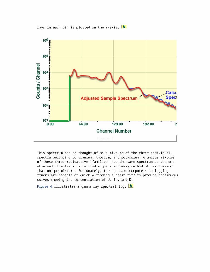
Figure 5

SN, LN AND LATERAL LOG BEHAVIORThe short normal log is widely used for geological correlation between wells; it also provides an approximate value of Rxo. The long normal and lateral logs are adapted to supply a reasonable value of Rt in thick beds. Very often, homogeneous resistive layers alternate with low resistivity beds. The tool response in thick resistive beds shows:

Poor bed definition (rounding off) when the bed thickness is smaller than the tool spacing AM

Apparent bed thickness smaller than actual thickness by an amount equal to AM.

A thin resistive layer is reflected by a depression together with two symmetrical peaks.

Further details on old electric logs are found in the References.

LATEROLOG OVERVIEWIn the 1920s, Conrad Schlumberger put forward the idea of a "guarded electrode" in an attempt to improve on the electrical logs of the time that had undesirable borehole effects. His idea was not put into practice until H. G. Doll designed a working guard electrode system. From this starting point, laterologs evolved in a number of ways. The laterolog-7, which used small guard electrodes, was later joined by the laterolog-3, which used long guard electrodes. Both used the same

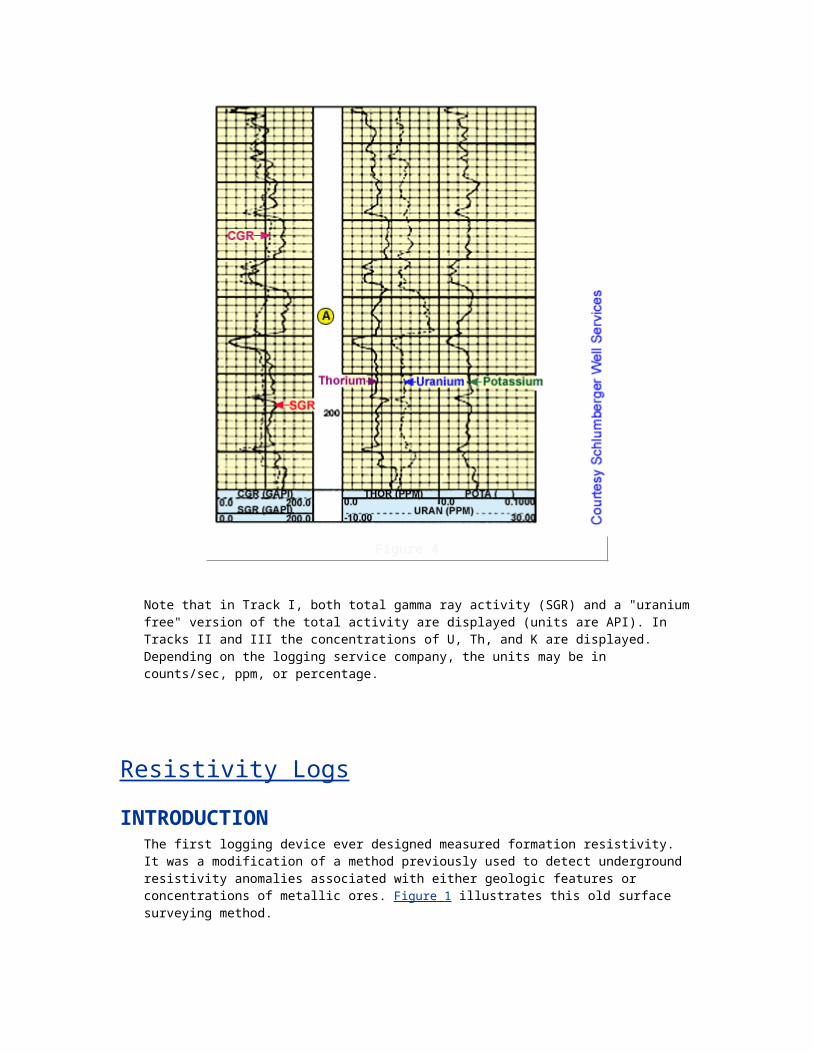
principle of a constant survey current (Io) being "forced" into the formation by bucking currents from guard electrodes. By monitoring the voltage required to maintain the fixed current Io, the formation resistivity was determined. The conductivity laterolog evolved from these tools. It maintained a constant voltage on the measure electrode while current variations monitored the formation conductivity.

Today, the laterolog tool most commonly used is the simultaneous dual laterolog. It is neither a conductivity nor a resistivity laterolog, but rather a hybrid using a constant product of current and voltage (constant power). The design of this tool solved many problems associated with earlier laterologs and it is now the standard basic resistivity log for salt mud environments.

WHEN TO USE A LATEROLOGLaterologs should be used when the following conditions exist:

There is seawater or brine mud in the hole.

The Rmf/Rw ratio is less than 3.

Hole size is less than 16 in.

Furthermore, the laterolog is superior to the induction log when Rt exceeds 150 m2/m. It also gives a better estimate of Rt than the induction log when bed thickness is less than 10-feet. Figure   1: Preferred Ranges for Application of Induction Logs and Laterologs provides specifics

concerning when to run a laterolog.

Figure 1

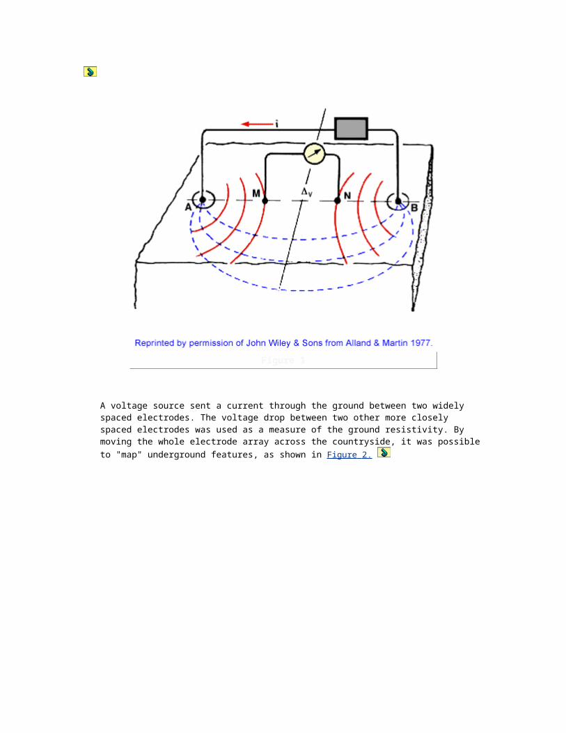
This Figure shows a plot of the Rmf /Rw ratio versus porosity (). The laterolog is preferred when the crossplot of Rmf /Rw versus falls on the left side of the chart.

LATEROLOG TOOLS (LL3, LL7 & DUAL LATEROLOG)Logging with laterologs was introduced to cope with salty mud. These muds have a very high conductivity, and consequently the effect of the borehole on resistivity measurements is also very high. The Laterolog technique is therefore complementary to the induction logging method, designed for oil-base mud which has hardly any conductivity at all.

LATEROLOG 3 (LL3)Figure   1 (Pattern of current flow from a long cylindrical electrode located in a homogeneous

medium) shows the principle of the focused current log.

Figure 1

On the left, a long electrode bar is shown imbedded in a homogeneous medium. The potential is constant all over the bar, and the current lines will run horizontally in the middle because current flow lines are perpendicular to equi-potential surfaces. The same principle is applied for the LL3 by using 3 bars, as shown at the right in the above graphic . The center bar is 1 foot long, and the two guard electrodes are 5 feet long. By keeping the potentials equal for all three electrodes, the current from the middle electrode is forced horizontally into the formation. This is even true when the bars are surrounded by a layer of mud with a resistivity that is much lower than the resistivity

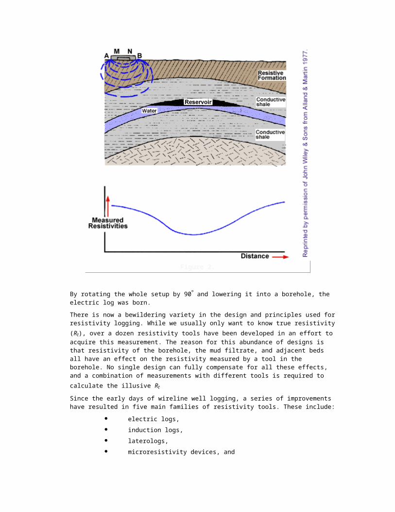
of the formation. The currents of the guards are adjusted to maintain the same potential as the center electrode, while the potential of the center electrode is kept at a fixed value. The ratio of the current and the potential of the center electrode is a good indication of the formation conductivity Ct.

LATEROLOG 7 (LL7)The laterolog 7 (LL7) is based on the same design as the LL3. In the LL3, the electrodes that carry very high currents (several amperes) are also used to measure potentials. This restricts the dynamic range of the measurements. In the LL7, two separate potential measuring electrode pairs are added, bringing the total to 7. The return electrode is positioned far away from the tool on the logging cable. This arrangement ensures that the current sheet penetrates the invaded zone and improves the measurement of the resistivity of the uninvaded zone.

DUAL LATEROLOGFigure   2 shows one version of the Dual Laterolog tool with its associated measure electrodes.

Figure 2

This tool is a combination of deep (LLd) and shallow (LLs) investigation devices. The principles adopted in the LL7 and LL3 have been combined in one tool, which features the 7 electrodes in its center and 2 large bucket electrodes positioned respectively above and below the series of 7.

In the LLd (deep) mode (left of Figure   3, The Dual Laterolog configuration), the surveying current Io , that flows from the center electrode, A0, is focused by bucket currents from electrodes A2 and

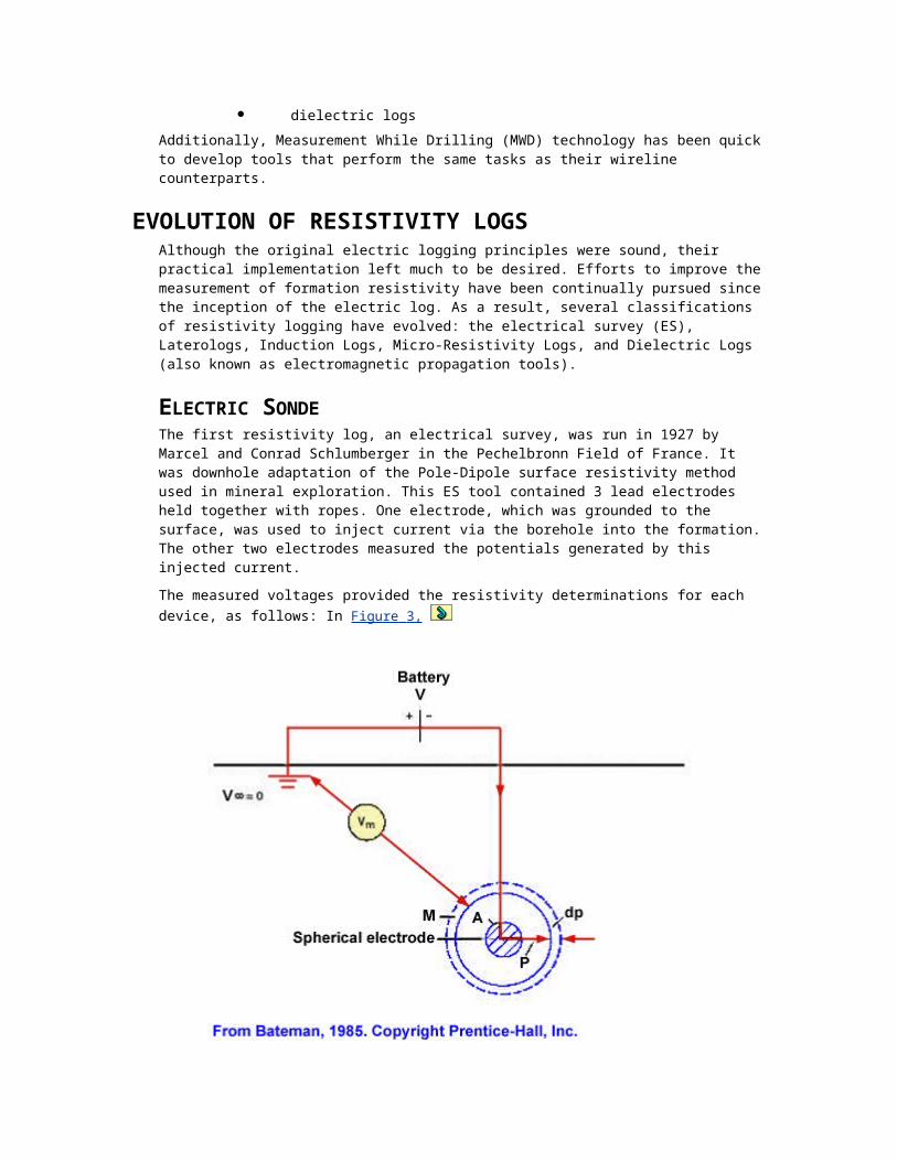
A2' supported by A1 and A1'.

Figure 3

The four "A" electrodes are all connected in this mode. This arrangement provides strong focusing deep into the formation. In the LLs (shallow) mode (right-hand part of the above graphic) the bucking currents flow from A1 to A2 and A1’ to A2’, reducing the depth of investigation. The electrodes are switched several times per second from one to the other configuration, and the two resistivity traces are produced simultaneously.

The dual laterolog measurements are often supplemented with a shallow resistivity measurement carried out with electrodes that are mounted in a pad that is pressed against the borehole wall to obtain Rxo. Figure   4 shows the current paths for the MSFL, which has five rectangular electrodes mounted on a pad carried on one of the caliper arms (refer to the discussion on Microresistivity Tools).

Figure 4

In this way, three resistivity measurements are obtained simultaneously with different radii of investigation. In addition to these resistivity measurements, auxiliary curves, such as caliper, gamma ray, and spontaneous potential curves, may be recorded. The resistivity curves are presented on a standard four-decade logarithmic scale (Figure   5).

Figure 5 .

Under the normal conditions found when using a dual laterolog, the radial profile of resistivities is as shown in Figure   6; i.e.,

Figure 6;

Rt > Rxo > Rm. Between the invaded zone and the undisturbed formation is a transition zone with a resistivity value between Rt and Rxo.

If a horizontal slice were made through the tool and its surrounding formation and examined in plan view, the image in Figure   7 would be seen.

Figure 7

Here the current flows radially outward from the tool, and has to pass through the mud, the invaded zone, and the undisturbed formation before arriving at the return electrode. The current, if held constant, thus develops a series of voltage drops across each zone encountered. The relationship between these voltages may be simplistically expressed as:

 Vtotal = Vmud + Vinvaded + Vundisturbed

 Each voltage drop is proportional to the product of the current, the resistivity of the zone, and some geometrical constant, depending on the size of the zone.

DUAL LATEROLOG "FINGERPRINTS"The characteristic behavior of the DLL tool in zones having movable hydrocarbons makes quick-look interpretation very simple. The golden rule is that the pattern in which RLLD > RLLS > RMSFL is a good indication that hydrocarbons are present, and conversely, the pattern in which RMSFL >

RLLS > RLLD is a good indication that the zone is wet (Figure   8).

Figure 8 .

Minimal separation between the curves suggests little or no invasion, and therefore indicates that the zone is impermeable (Figure   9).

Figure 9 .

Likewise, any relative ordering of the curves other than the two cases above suggests little or no invasion and would therefore indicate that the zone is impermeable.

BOREHOLE AND INVASION CORRECTIONSCorrections to the raw data may be necessary when hole size or depth of invasion exceed optimum parameters for the tool. For older logs, charts are available from wireline service companies to make such corrections, and these charts will help you to determine when such corrections will be needed for the particular logging tool you are using. Each company has its own charts, and corrections from one company's charts should not be used to correct readings obtained from logging tools of a different company.

The MSFL, a pad contact device, is sensitive to mudcake thickness (hmc) and mudcake resistivity (Rmc).

In the range of normal interest, when laterolog readings lie in the range of 10 < (RLL/Rm) < 100, all corrections are within ±10%. Where hole diameters are large, however, the LLs correction can become intolerably large.

Once raw log readings have been corrected for borehole effects, they may be corrected for invasion effects, using what is commonly known as a butterfly chart (Figure   10).

Figure 10 .

This chart plots the ratio of RLLD/RLLS against the ratio of RLLD/Rxo. There are three families of lines on the chart. They are constant values of Rt/RLLD constant values of Rt/Rxo, and constant values of di.

In order to use the chart, it is first assumed that (RMSFL)cor is equal to Rxo. A point is then located on the chart at the coordinates RLLD/RLLS and RLLD/RMSFL. This point uniquely defines the three unknowns: Rt, Rxo, and di.

The lower left portion of the chart corresponds to the invasion pattern RMSFL > RLLS > RLLD, which usually occurs in water-saturated zones where Rmf > Rw.

LOG QUALITY CONTROLDeep and shallow laterolog curves should read the same in impermeable formations (shales and evaporites). In porous and permeable zones, some separation between the two laterolog curves is to be expected, depending on the invasion diameter and the ratio of Rxo to Rt.

ANOMALOUS LATEROLOG BEHAVIORThe early laterologs were prone to various types of anomalous behavior, which are chronicled here to give some insight into the few anomalies that can still occur, even with the dual laterolog. This information may also be helpful in the event that you are called upon to analyze old well data.

THE DELAWARE EFFECT

During the early 1950s in the Permian basin, logging engineers found that laterologs behaved anomalously when approaching a thick resistive bed, such as the massive anhydrite and salt that overlies the Delaware sand. The effect manifested itself by a gradual increase in apparent resistivity, starting when the bridle entered the highly resistive bed. Apparent resistivities would climb to as much as 10 times the value of Rt before the sonde itself entered the highly resistive bed. The solution for the laterolog 7 was to place the B return electrode at the surface. For the conductivity laterolog, the solution was not so easy, since these devices were using a 280 Hz survey current generated in the cartridge. Having the return at the surface did not solve the problem, since skin effect restricted the return current to a sheath around the borehole, thus resulting in the effective return electrode as the lower part of the cable (Figure   1).

Figure 1 .

Compensation for this effect with the Laterolog 3 involved a complicated setup, with two sondes -one on each side of a cartridge, and a B return electrode on the bottom. However, for all practical purposes, the laterolog 3 remains susceptible to the Delaware effect.

THE ANTI-DELAWARE EFFECTIn an attempt to improve on the situation and provide a dual spacing laterolog, a tool was introduced with both deep and shallow devices. However, this device also behaved anomalously beneath highly resistive beds. The deep laterolog showed a gradient of decreasing resistivity - the exact opposite of the Delaware effect. With the B electrode at the surface (effectively at zero potential), the N electrode acted as the takeoff point of a potential divider formed by the borehole below and above N; thus the approaching sonde, at some positive potential, would cause N to

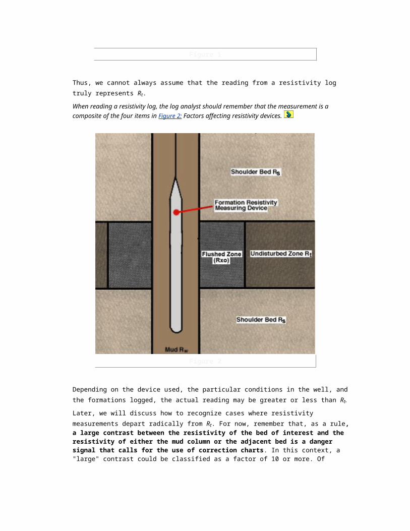
raise its potential. The anti-Delaware effect would at worst cause a 50% reduction in the deep laterolog and would only be noticeable within 35 ft of the resistive bed. In fact, the effect had been present on the earlier B electrode at surface, Delaware-free laterologs, but it had not been noticed since there was no shallow laterolog with which to compare the deep laterolog.

The dual laterologs in use today have incorporated features that assure virtual freedom from Delaware and anti-Delaware effects. However, a new effect has been observed on the dual laterolog, again associated with highly resistive beds.

THE GRONINGEN EFFECTThe Groningen effect, first observed in the course of logging gas wells in Holland, manifests itself as the LLd reading too high when the N electrode enters a highly resistive bed. From a distance of AN below the bed boundary (about 102 ft), the LLd will rise over a short distance to an anomalously high value, which it will then maintain until the bed is entered. Experiments have shown that the effect depends on the operating frequency, and is only troublesome in low-resistivity formations immediately below a massive salt or anhydrite bed. Modern laterolog devices can detect and correct for the Groningen effect.

The Groningen effect appears (if at all) within 102 ft (31 m) of a resistive bed and will be of interpretive importance only where Rt in the underlying bed is less than 10 m2/m. It can appear even if casing is set to the bottom of the resistive bed.

DUAL LATEROLOG "NORMAL" ANOMALIESDual laterologs experience environmental effects, even if resistive bed effects do not occur. A tool has not yet been designed that is entirely free of the disturbing effects of the borehole and adjacent beds, although progress has been made in reducing these effects. For interpretive work, these environmental effects must be taken into account. The hole size and invasion effects have already been covered in the previous discussions, and another set of corrections is worth noting.

SHOULDER BED CORRECTIONS -SQUEEZE AND ANTI-SQUEEZE

When the sonde is in front of a bed with a resistive shoulder on either side, the current tends to concentrate in the least resistive path; in other words, it is "squeezed" between the resistive shoulders into the formation of interest. Charts are available to correct for this effect. The correction factor to be applied to the borehole corrected log reading is a function of bed thickness and the contrast between the apparent reading and the shoulder resistivity Ra /Rs. Where this factor is less than one, a squeeze situation exists and the apparent log reading is too high. Where Ra /Rs is greater than one, the bed is surrounded by a conductive shoulder and the current tends to fan out into the path of least resistance--the conductive shoulders. Since this is the reverse of "squeezed," it is called "anti-squeeze." The apparent log readings are too low in this situation.

The LLd is much more affected by squeeze and anti-squeeze than is the LLs -even in what might be considered thick beds (50 ft or more). When making detailed interpretations, one should use the Shoulder Bed Correction Charts for LLd after borehole correction and before any other step. Invasion corrections may then be made.

A word of caution is in order. In general, an ideal laterolog has a depth of investigation response that behaves logarithmically with respect to invasion diameter, but it is also a function of the contrast between Rxo and Rt .

Furthermore, the effect of a hole larger than 8 in. (20.32 cm) is to replace part of the Rxo zone by mud, thus changing the effective position of the origin on the invasion correction chart.

ANOMALOUS LATEROLOG BEHAVIOR

The early laterologs were prone to various types of anomalous behavior, which are chronicled here to give some insight into the few anomalies that can still occur, even with the dual laterolog. This information may also be helpful in the event that you are called upon to analyze old well data.

THE DELAWARE EFFECTDuring the early 1950s in the Permian basin, logging engineers found that laterologs behaved anomalously when approaching a thick resistive bed, such as the massive anhydrite and salt that overlies the Delaware sand. The effect manifested itself by a gradual increase in apparent resistivity, starting when the bridle entered the highly resistive bed. Apparent resistivities would climb to as much as 10 times the value of Rt before the sonde itself entered the highly resistive bed. The solution for the laterolog 7 was to place the B return electrode at the surface. For the conductivity laterolog, the solution was not so easy, since these devices were using a 280 Hz survey current generated in the cartridge. Having the return at the surface did not solve the problem, since skin effect restricted the return current to a sheath around the borehole, thus resulting in the effective return electrode as the lower part of the cable (Figure   1).

Figure 1 .

Compensation for this effect with the Laterolog 3 involved a complicated setup, with two sondes -one on each side of a cartridge, and a B return electrode on the bottom. However, for all practical purposes, the laterolog 3 remains susceptible to the Delaware effect.

THE ANTI-DELAWARE EFFECT

In an attempt to improve on the situation and provide a dual spacing laterolog, a tool was introduced with both deep and shallow devices. However, this device also behaved anomalously beneath highly resistive beds. The deep laterolog showed a gradient of decreasing resistivity - the exact opposite of the Delaware effect. With the B electrode at the surface (effectively at zero potential), the N electrode acted as the takeoff point of a potential divider formed by the borehole below and above N; thus the approaching sonde, at some positive potential, would cause N to raise its potential. The anti-Delaware effect would at worst cause a 50% reduction in the deep laterolog and would only be noticeable within 35 ft of the resistive bed. In fact, the effect had been present on the earlier B electrode at surface, Delaware-free laterologs, but it had not been noticed since there was no shallow laterolog with which to compare the deep laterolog.

The dual laterologs in use today have incorporated features that assure virtual freedom from Delaware and anti-Delaware effects. However, a new effect has been observed on the dual laterolog, again associated with highly resistive beds.

THE GRONINGEN EFFECTThe Groningen effect, first observed in the course of logging gas wells in Holland, manifests itself as the LLd reading too high when the N electrode enters a highly resistive bed. From a distance of AN below the bed boundary (about 102 ft), the LLd will rise over a short distance to an anomalously high value, which it will then maintain until the bed is entered. Experiments have shown that the effect depends on the operating frequency, and is only troublesome in low-resistivity formations immediately below a massive salt or anhydrite bed. Modern laterolog devices can detect and correct for the Groningen effect.

The Groningen effect appears (if at all) within 102 ft (31 m) of a resistive bed and will be of interpretive importance only where Rt in the underlying bed is less than 10 m2/m. It can appear even if casing is set to the bottom of the resistive bed.

DUAL LATEROLOG "NORMAL" ANOMALIESDual laterologs experience environmental effects, even if resistive bed effects do not occur. A tool has not yet been designed that is entirely free of the disturbing effects of the borehole and adjacent beds, although progress has been made in reducing these effects. For interpretive work, these environmental effects must be taken into account. The hole size and invasion effects have already been covered in the previous discussions, and another set of corrections is worth noting.

SHOULDER BED CORRECTIONS -SQUEEZE AND ANTI-SQUEEZE

When the sonde is in front of a bed with a resistive shoulder on either side, the current tends to concentrate in the least resistive path; in other words, it is "squeezed" between the resistive shoulders into the formation of interest. Charts are available to correct for this effect. The correction factor to be applied to the borehole corrected log reading is a function of bed thickness and the contrast between the apparent reading and the shoulder resistivity Ra /Rs. Where this factor is less than one, a squeeze situation exists and the apparent log reading is too high. Where Ra /Rs is greater than one, the bed is surrounded by a conductive shoulder and the current tends to fan out into the path of least resistance--the conductive shoulders. Since this is the reverse of "squeezed," it is called "anti-squeeze." The apparent log readings are too low in this situation.

The LLd is much more affected by squeeze and anti-squeeze than is the LLs -even in what might be considered thick beds (50 ft or more). When making detailed interpretations, one should use the Shoulder Bed Correction Charts for LLd after borehole correction and before any other step. Invasion corrections may then be made.

A word of caution is in order. In general, an ideal laterolog has a depth of investigation response that behaves logarithmically with respect to invasion diameter, but it is also a function of the contrast between Rxo and Rt .

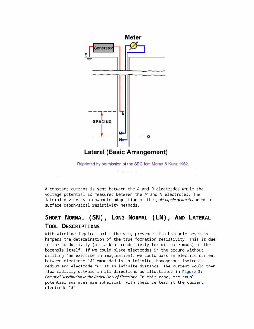
Furthermore, the effect of a hole larger than 8 in. (20.32 cm) is to replace part of the Rxo zone by mud, thus changing the effective position of the origin on the invasion correction chart.

INTRODUCTION TO INDUCTION TOOLS Logging systems used before the introduction of induction logging depended on the presence of an electrically conductive fluid in the borehole to transmit electric current to the formation. In many rotary drilled wells, the drilling fluid is a water-base mud that conducts electricity. However, some wells are drilled with nonconductive fluids, such as oil-based muds, air, and gas. Under such conditions, it is impossible to obtain a satisfactory electrical log using conventional electric logging tools.

Induction logging does not depend upon physical contact between the walls of the wellbore and the logging tool. The induction logging tool acts like a transformer: the transmitter coil is energized with alternating current, which induces in the formation a secondary current that is proportional to the electrical conductivity of the formation and to the cross-sectional area affected by the energizing coil. The higher the conductivity of the formation, the lower the resistivity, and the larger the formation current will be. This current in turn induces a signal into a receiver coil, the intensity of which is proportional to the formation current and conductivity. The signal detected by the receiver coil is amplified and recorded at the surface.

The direct measurement is therefore one of conductivity. Both the conductivity and reciprocated conductivity (resistivity) curves are shown on the log. The deflections of these curves are proportional to formation conductivity. Formations having resistivities of 10, 100, or 1000 ohm-m would have conductivities of 100, 10, and 1 mmho/m, respectively.

Induction logging equipment records formation conductivity over a wide range. The accuracy is excellent for conductivity values higher than 20 mmho/m (resistivity values less than 50 ohm-m) and is acceptable in lower conductivity ranges (down to 5 mmho/m). Beyond this limit, the induction log continues to respond to formation conductivity variations, but with diminished accuracy. There is a small uncertainty of about ±1 mmho/m on the zero of the present equipment.

WHEN TO USE AN INDUCTION LOGInduction logs are recommended when:

the hole to be logged is filled with fresh water or

the hole to be logged is filled with oil-base mud

the hole to be logged was air drilled

the Rmf/Rw ratio is greater than 3

the Rt is less than 150 ohm-m and bed thickness is greater than 30 feet.

The induction log is the only resistivity device that works in oil-based mud (where oil is the continuous phase) or air-filled holes. The laterolog measurement is preferred when Rmf/Rw falls to the left of the vertical dashed line and to the left of the solid line for the appropriate value of Rw (Figure   1: Preferred conditions for induction tools). The induction log is preferred above the

appropriate Rw line.

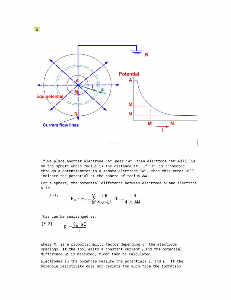
Figure 1

To the right of the dashed line and below the appropriate Rw curve, either or both logs may be required for an accurate interpretation.

TOOL TYPESTwo commonly used induction tools are the single-and dual-induction devices. Each of these tools can be combined with the other sensors, thereby allowing both porosity and resistivity logs to be recorded simultaneously. Figure   2: Induction-Sonic tool combination shows a typical tool string.

Figure 2

PRESENTATIONS AND SCALESInduction logs and combination induction logs are recorded on a variety of scales and presentations. The primary measurements of conductivity are always recorded on a linear scale when presented. In contrast, resistivity can be plotted on a linear or logarithmic scale. When porosity data are presented, a split grid is usually employed. Figure   3 (Linear induction log

presentation), Figure   4

Figure 4

(Logarithmic induction log), and Figure   5

Figure 5

(Split grid induction log) illustrate the various possibilities.

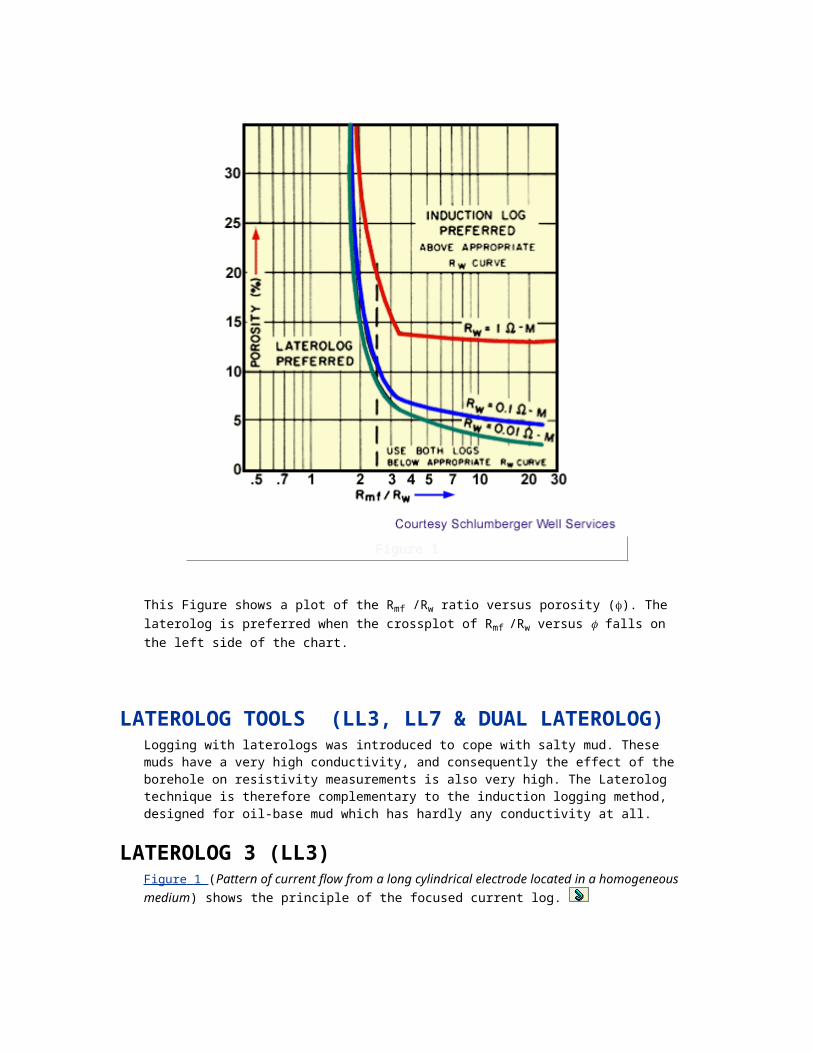
Figure 3

INDUCTION PRINCIPLESThe induction tool works best when the borehole fluid serves as an insulator, such as air or gas. Though originally designed for resistivity recording in wells drilled with non-conductive fluids, the induction log has actually found wide application in holes drilled with fresh-and oil-based muds. This tool has been shown to work well when the borehole contains conductive mud, unless:

the mud is too salty,

the formation too resistive (above 150 ohm-m), or

the borehole diameter too large.

The sonde contains at least 3 coils, one transmitter and two receiver coils, however, the principle can be understood clearly by considering a sonde with only one transmitter coil and one receiver coil (Figure   1: Basic two-coil induction log system). The transmitter sends out an alternating

current with a constant frequency of 20 kHz.

Figure 1

The alternating magnetic field generated by the primary coil induces secondary ground current loops into the formation. These loops in turn create magnetic fields, which induce currents in the receiver coils. Because the alternating current in the transmitter coil is of constant frequency and amplitude, the amplitude of the secondary field is proportional to the conductivity of the formation. (The voltage induced in the receiver coil is proportional to the ground loop currents and, therefore, to the conductivity of the formation.) The two receiver coils R1 and R2 are wound in opposite directions to compensate the direct coupling between T and R1. Actual logging tools contain 4 to 16 coils, of which the signals are combined to improve the vertical resolution as well as obtain a range of investigation depths (focusing).

Calibration of the system is a two-step process. First, the tool is suspended high off the ground away from any conductive materials. Since the tool is in a zero-conductivity environment, it is adjusted to read zero conductivity (infinite resistivity). Second, a circular loop or ring of a known conductivity (known resistivity of either 1 or 2 ohm-m) is placed on the tool. The tool response is now adjusted to measure this "calibration" value.

Now, with the two end points defined and measured (the high end simulated by the tool in air and the low end simulated by the test loop), the tool is capable of measuring most normally encountered resistivity or conductivity values found in the oil-field.

Of course, when the tool is at the bottom of a l0,000-ft well, there is no way a test loop can be placed around the sonde, so an internal calibrator is included in the tool. The calibrator will have a nominal value of 1 or 2 ohm-m; its precise value is determined monthly by reference to the test loop. These internal calibrators shift with age but behave reasonably well under normal use. A check of the zero conductivity point when the tool is in the hole is accomplished by simply opening the receiving coil. Any extraneous signal is canceled out by a zero adjustment.

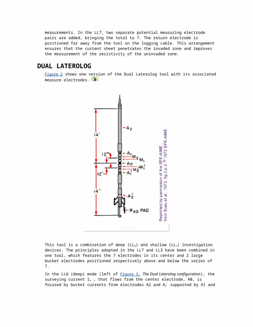
SKIN EFFECTLinkage of each ground loop with its own magnetic field (a ground loop has self-inductance), and with the magnetic fields of the other nearby ground loops creates a cross-coupled system. This results in eddy currents that require a more advanced treatment of EM theory than what has been discussed. That is, it cannot be assumed that the individual ground loops are independent of one another. It can be predicted that, with increasing distance from the source (i.e., transmitter coil), there will be attenuation in the amount of transmitted power because

1. The dissipation of energy by the flow of eddy currents in the region near the source decreases the energy available for transmission to regions farther out.

2. Regions far from the source are shielded from the magnetic field of the transmitter coil by the annulling effect of magnetic fields of opposite sign from the eddy currents in the conductive medium closer to the transmitter. In a sense, the "shielding" of the outer regions is equivalent to a reflection of the energy back toward the source.

As a consequence of these interactions, there is a reduction in the receiver-coil signal; i.e., a reduction in high conductivity. This reduction is commonly called a skin effect.

Thus, if g is the conductivity reading observable in a given configuration of media without skin effect and a is the conductivity actually observed, then the difference, s, is the skin effect.

 s = g - a

 An amount, s is added to the observed reading by means of a skin effect compensating network. It is nonlinear and can best be illustrated by Figure   2: Correction of Formation Conductivity for Skin Effect. In practical terms, the tool reads a resistivity that is too high unless the skin effect compensation is applied.

Figure 2

ENVIRONMENTAL EFFECTSIn addition to the transmitting and receiving coils of the simple two-coil device (Figure 1: Basic Two-Coil Induction Log System) a practical field tool also includes additional focusing coils (Figure   3: Schematic Diagram of a Typical Induction Logging System ). These focusing coils make the current ground loop flow as far away from the borehole as possible to help eliminate borehole and drilling-mud-filtrate invasion effects.

Figure 3

BED THICKNESS CORRECTIONSUnfortunately, a tradeoff has to be made when designing an induction tool. Good bed resolution can only be obtained with closely spaced transmitter-receiver coil arrangements, but this close spacing results in a relatively shallow radial depth of investigation. Conventional induction devices, designed for deep investigation, have poor vertical bed resolution. Effectively, the signal received is a mixture of signals from points both above and below the horizon being measured.

The surface control equipment offsets the poor bed resolution characteristic by emphasizing the zone of interest and playing down the measurement made on either side of the horizon (Figure   4:

Vertical Response of the Induction Tool ).

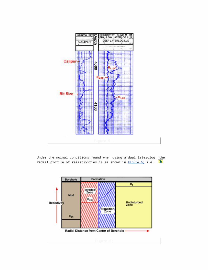
Figure 4

The electronic circuitry used in this tool can manipulate three measurements in such a way that the reading recorded on the log is equal to a "weight" value A times the value of the interval being measured plus B times the values at points 78 inches above and below the point being measured. The values for A and B should be chosen so that A -2B = 1. This is logical: in a homogeneous formation where all three measurements are the same, the net effect is similar to the gross effect. This scheme assists in correcting the log for the effects of adjacent beds.The enhanced "phasor" processing of induction tool signals allows for improved bed thickness response.

INDUCTION CURRENT PATHSCurrent loops flow around the borehole in a horizontal plane. The measured signal includes signals from the mud, the filtrate invaded zone, and the undisturbed zone. The tool "sees" these three resistances as if they are in parallel (Figure   5: Induction Current Paths).

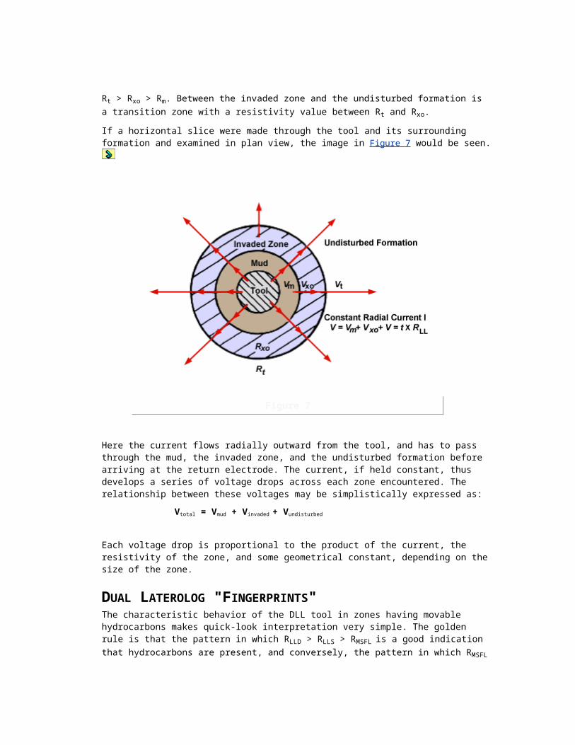
Figure 5

HOLE SIZE CORRECTIONSThe borehole effects due to the current loop in the mud can be corrected by using a special chart. The size of the correction is insignificant in fresh, resistive muds, but quite significant in salty, conductive muds.

If a SFL (spherically focused log) is run in conjunction with an induction log, a hole size correction is also needed. Figure   6: Borehole Correction Chart for the Sperically Focused Log (SFL) shows

the magnitude of corrections to be applied for this purpose.

Figure 6

The RSFL/Rm ratio is plotted against the ratio of (RSFL)cor to RSFL. The lines on the chart are for different hole sizes.

INVASION EFFECTS

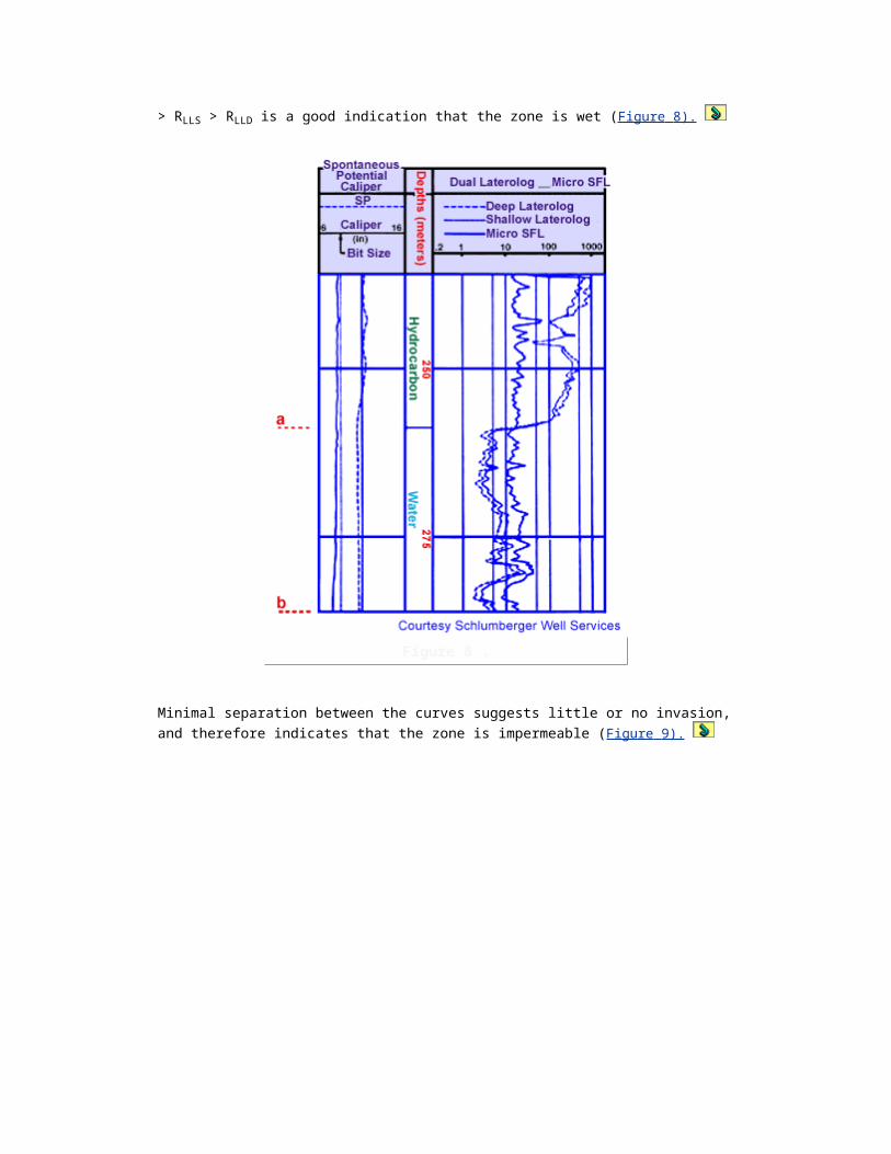
The "integrated radial geometric factor," or "G" describes the radial response of the induction tool. The G factor reveals which fraction of the measured signal comes from which radial distance from the tool. Mathematically, it can be described by the equation:

 txoID R

G1

R

G

R

1

 If di (the diameter of invasion) is small, then G is small and the entire signal will come from the undisturbed zone; in this case, RID is equal to Rt. If di is large, then G also is large and a large part of the total signal will come from the filtrate-invaded zone. In this case, RID reads somewhere between Rt and Rxo.

Figure   7 : Induction Geometry Factor (G) shows G as a function of di for the deep induction tool.

Figure 7

This plot can be used to solve the following case. Suppose di is 80 in., Rxo = 20, and Rt = 10. What will the induction tool read? From the above Induction Geometry Factor graphic, G for a di of 80 inches is 0.4.

Therefore, the equation given above can be written as:

  08.06.002.010

)4.01(

20

4.0

R

1

ID

 

RID = 1/0.08 = 12.5

Thus, RID reads greater than Rt.

Figure   8: Radial Distribution of Fluids in the Vicinity of the Borehole,

Figure 8

Oil-Bearing Formation (Qualitive) illustrates a typical invasion pattern with high filtrate saturation in the invaded zone and low connate water saturation in the undisturbed zone.

It should be realized that this treatment of the invasion problem is the reverse of what is encountered in the field; i.e., in practice Rxo, Rt, and di are not known in advance. The objective is to find Rxo, Rt, and di from the measured log values. In fact, if only the value of RID is known, there is no solution to the problem. If three unknowns exist, then three known quantities are needed to solve the problem. The solution is to use the dual induction SFL combination-logging tool. Since the geometric factor for the medium induction log (G’) is different from the geometric factor for the deep induction log (G) at the same di, the following three equations can be solved simultaneously:

 txoID R

G1

R

G

R

1

txoIM R

'G1

R

'G

R

1

RSFL = f (Rxo)

 

TOOL CALIBRATIONInduction tool calibration can be performed on land at any time. The sonde is placed in a zero conductivity environment. This is normally done by raising the sonde up in the air well away from metallic objects. This defines a zero point. A calibration loop is then placed around the sonde to give a known conductivity signal, usually 500 mmhos. This calibration is performed on a monthly basis. It is almost impossible to perform on an offshore rig because of the surrounding metal structure. In cases where it is not possible to set the zero point under controlled conditions at the surface, it is permissible to set it with the tool in the hole opposite a thick, very highly resistive zone (salt, anhydrite, dense low-porosity carbonate, etc.) if one exists. The sonde and its associated electronic cartridge form a matched set and should always be used together.

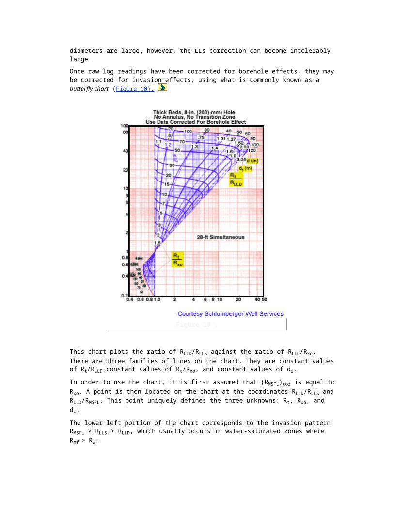
MICRORESISTIVITY TOOLSMicroresistivity devices are characterized by short electrode spacings of only a few inches. This limits such tools to very shallow depths of investigation. Microresistivity tools are useful in determining the following:

flushed zone saturation, Sxo

residual oil saturation, (ROS) hydrocarbon movability

hydrocarbon density, rhy

invasion diameter, di invasion corrections to deep resistivity devices

With their shallow depths of investigation, micro-resistivity tools usually provide a good approximation of the resistivity of the flushed zone (Rxo). A variety of tools, old and new, have been used over the years; each with its own special characteristics. The following list covers the majority of the microresistivity devices that are now, or have been, widely used. These tools can be divided into two main groups: the mandrel tools and the pad contact tools.

Mandrel Tools:

 

Log Type

 16-in. SN

 

Short Normal

 LL8

 

Laterolog 8

 SFL

 

Spherically Focused Log

 Pad Contact Tools:

 

Log Type

 MLL

 

Microlaterolog

 PL

 

Proximity Log

 MSFL

 

Microspherically Focused Log

 ML

 

Microlog

 

The mandrel tools are constructed with electrodes on a cylindrical mandrel. Such tools do not require physical contact with the formation. In contrast, the pad contact tools have their electrodes embedded in an insulating pad carried on a caliper arm that is forced against the borehole wall. The general principles of all these tools may be understood through a discussion of the ML and MFSL logging devices.

MICRO-RESISTIVITY PAD DEVICES

MICROLOG (ML)

Though the microlog was one of the first microresistivity devices on the market and has had a spectacular career, it has nonetheless tended to be under utilized. Originally, it was used as a pseudo-porosity device. When that function was improved with modern porosity devices, the microlog was relegated to the pile of has-beens within the logging industry. However, it is valuable as a tool that offers superb visual identification of porous and permeable zones. Figure   1 shows a microlog and proximity log presentation.

Figure 1

The presence of permeability is indicated wherever the normal curve reads higher than the microinverse curve, and the microinverse curve reads close to Rmc.

The microlog records two resistivity curves, each having a shallow depth of investigation. The microlog looks for a resistivity contrast between the mudcake and the flushed zone. Any formation having no porosity or permeability will not be able to promote mud filtrate invasion, and will therefore show no mudcake buildup. Hence, there will be no positive separation between the two resistivity curves.

This tool has 3 small button-shaped electrodes that are embedded in a rubber pad (Figure   2: The

Microlog Principle).

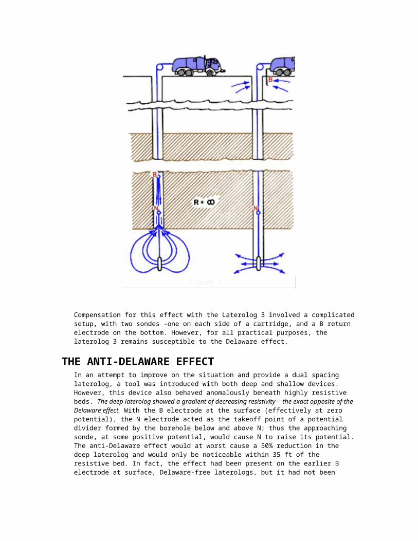
Figure 2

The electrodes are placed in a vertical line with a spacing of 1 inch between successive electrodes. An electrical current of known intensity is emitted from Ao, and the differences in

electrical potential are measured between M1 and M2, and between M2 and a surface electrode.

The resulting 2 curves represent a 2-inch normal and 1-inch "inverse" recording, with important chjaracteristics:

The radius of investigation is smaller for the inverse curve, which is therefore strongly affected by the mudcake.

The normal curve reads 2 to 3 inches deep into the formation, and is therefore more affected by the invaded zone.

The mudcake usually has a lower resistivity than the permeable beds, so the "inverse curve" will therefore read a lower value than the normal. Consequently, the ML indicates the presence of mudcake by showing a separation between the 2 resistivity traces and thereby delineates permeable beds. Figure   3: Example of a Microlog and Proximity Log shows a microlog and a

proximity log.

Figure 3

The separation of the micro-normal and micro-inverse curves clearly delineates the vertical extent of the permeable bed. This is confirmed by the separation between the caliper and the nominal bit size, which can be used to show the thickness of the mudcake across this interval. The larger electrode spacing of the proximity tool causes the proximity curve in the Microlog and Proximity Log graphic to show less vertical resolution and a deeper horizontal investigation than the ML curves. For this reason, a proximity tool’s resistivity values are often representative of the transition zone resistivity, Ri. The ML is the best of all micro devices for making "sand counts".

MICRO SPHERICALLY FOCUSED LOG (MSFL)Being a pad mounted version of the Spherically Focused Log (SFL), the Micro Spherically Focused Log (MSFL) is typically incorporated in the dual laterolog, DLL-Rxo tool. Its design is based on the concept that accurate resistivity data is best obtained when the potential distribution around the current-emitting electrode is spherical. This condition has been approximated by an array of concentric electrodes that resembles the Dual Laterolog in cross section, as depicted in Figure   4: Schematic Diagram of the Dual Laterolog-Rxo Tool. It is probably no coincidence that both tools contain 9 electrodes.

Figure 4

In this case, both the investigating current Io and the bucking current I1 are emitted through center electrode Ao. The sum of these two currents is adjusted by varying the potential of electrodes A1 and A2 in such a way that the measured voltage at Mo is kept equal to a constant reference voltage. The investigating current Io is roughly proportional to the conductivity of the slice of the formation filled with section lines seen in Figure   5: Micro-SFL Principle.

Figure 5

The main advantage of the MSFL over the micro-log is that it is much less affected by the mudcake and therefore provides a better estimate of the flushed zone resistivity Rxo, which is derived with the following relation :

 

O

1

IM

EMo

E

xoR

 

DEPTH OF INVESTIGATIONEach microresistivity tool has its own characteristic depth of investigation. It is important to know these values in order to select the tool with the right characteristics for the job. A tool with a shallow depth of investigation is needed if invasion is shallow and the tool is to read Rxo without undue influence from Rt. Conversely, where there is deep invasion, a deep investigation tool will ensure a reading of Rxo that is free from effects from Rmc.

As with other tools, no single value for the depth of investigation can be used. Rather, a pseudogeometric factor must be used. The pseudogeometric factor indicates how much of the total tool signal is received from an annular formation volume represented by distances (expressed in inches) from the borehole wall (Figure   6: Depth of Investigation for Microresistivity Tools).

Figure 6

BED RESOLUTIONNot only does each of the microresistivity tools have their own characteristic depth of investigation, each tool also has its own characteristic bed resolution; i.e., some tools are better than others at distinguishing thin beds. Tools with coarse bed resolution values are "blind" to thin shale and/or sandstone layers. For example, 3-inch shale streaks will not be "seen" by a short normal log but may easily be delineated by a microlog. By way of contrast, a shallow-focused log, depending on its electrode spacing, may be able to resolve beds 1 or 2 feet thick at best.

ENVIRONMENTAL CORRECTIONSMicroresistivity devices of the mandrel type are subject to aberrations caused by well bore size. These effects can be quite severe. The pad contact tools, however, are only affected by excessive mudcake buildup, hole rugosity, and fractures.

By using the appropriate charts, one can make mudcake corrections. These charts are available from the wireline service companies and relate a correction factor to the mudcake thickness and resistivity. The mudcake thickness is calculated as half the difference between the bit size and the measured caliper reading when the caliper reads less than bit size.

For the mandrel-type tool, additional corrections must be made using service company charts that relate the log reading, the mud resistivity (Rm), and the hole size.

Sxo and Hydrocarbon Movability

The water (filtrate) saturation in the flushed zone (Sxo) may be estimated by using Archie’s equation

(Sxo)n = F . Rmf/Rxo

where

F = Formation Factor = a/m

To solve this equation, the following values must be known:a (tortuosity factor),

m (cementation exponent),n (saturation exponent),porosity),Rmf (resistivity of the mud filtrate -corrected for formation temperature), and Rxo (resistivity of the flushed zone).

The value of Sxo may not reveal much about the amount of oil in place, but it will reveal a great deal about whether the oil in place is likely to flow or not. The invasion process acts like a miniature waterflood. Invading filtrate displaces not only connate water, but also any movable hydrocarbons. In the undisturbed state at initial reservoir conditions, the fractional pore volume occupied by oil is (1 -Sw). After filtrate invasion has taken place, the fractional pore volume occupied by oil is (l -Sxo). The difference between these two values is the fractional pore volume that contained movable oil. Figure   7: Hydrocarbon Movability shows this process.

Figure 7

The pore volume fraction of movable oil is determined by the relationship (Sxo -Sw). The fraction of the original oil in place that has moved is determined by:

(Sxo -Sw) / (1 -Sw)

This index can then be used as a measure of the quality of the pay. In formations where the relative permeability to oil is low, Sxo is likely to be close to Sw and the index will be low. This same formation will not be as productive as another with the same value of Sw but better relative permeability to oil and hence a higher value of Sxo.

HYDROCARBON DENSITYThe computation of hydrocarbon density in a pay zone can provide key information when there is doubt about the type of hydrocarbon present; i.e., does the formation contain oil, light oil, condensate, or gas? Since the porosity tools make their measurements in the flushed zone, they "see" a bulk volume of hydrocarbon equal to (1 -Sxo). This leads to the interesting paradox that where hydrocarbons are movable, they will have been flushed away from the zone where they can be seen. Thus large hydrocarbon effects on porosity tools may be misleading and really only indicate large volumes of residual hydrocarbons. A lack of pronounced hydrocarbon effects could mean either that movable hydrocarbons are present or the formation is wet. Either way, a good value of Sxo is essential for correct prediction of hydrocarbon density and hence the type of hydrocarbon present in the formation.

QUALITY CONTROLQuality control for these devices can be summarized by the following maxims:

Beware of washed-out holes because (a) pad contact tools lose contact with the formation and "float" in the mud column and (b) mandrel tools give severely inaccurate readings.

Beware of thick mudcakes because pad contact tools require large corrections.

If hole conditions are bad, forget about trying to measure Rxo, because either the tool will stick or the pad will tear up. Either way, no usable log reading will be obtained.

Pad contact resistivity devices do not measure accurately in oil-base mud.

Dielectric Logs

PRINCIPLES OF DIELECTRIC TOOLS

INTRODUCTIONThe dielectric constant of a material affects the way in which an electromagnetic wave passes through it. Since the dielectric constants of oil and water are different, the behavior of electromagnetic waves in reservoir rocks is of interest to well loggers. Two classes of tools are available for measuring the formation dielectric constant:

Low-Frequency Tools use coils on a mandrel and operate at tens of megahertz;

High-Frequency Tools use microwave antennae on a pad contact device.

These two types will be considered separately. Examples of such tools are:

Electromagnetic Propagation Tool (EPT) (Schlumberger)

Dielectric Constant Log (DCL) (Halliburton)

Deep Propagation Tool (DPT) (Schlumberger)

The first of these is a very high frequency tool, the other two not so high.

Traditionally, the measurement of the conductivity or resistivity of a formation has been one of the main surveys performed in a borehole, primarily to determine water saturation. However, a second electrical characteristic of the formation can be measured--the dielectric permittivity. Dielectric logging devices can determine formation saturations from data dependent on the dielectric permittivity. The basic measurements are of the propagation time and the attenuation of an electromagnetic wave as it passes through a specific interval of formation.

EPTThe high-frequency tool is known as the electromagnetic propagation tool (EPT). Its basic measurements are of propagation time and the attenuation of a 1.1 GHz electromagnetic wave as it passes through a specific interval of formation. Because the propagation time in water is substantially higher than that in hydrocarbons, the EPT measurement is affected primarily by the water-filled porosity. This is in contrast to the nuclear porosity tools, which are influenced by the total porosity. In addition, for a wide range of salinities, the propagation time in water is practically constant and so saturation estimations can be made without prior knowledge of the resistivity of the formation water. When other openhole log data are available it is possible to distinguish between oil, gas, and water in reservoirs with unknown or changing Rw.

Physical PrincipleThere has long been a need for a method to determine water saturation that is less dependent on knowledge of water salinity. One such method is the measurement of dielectric permittivity. Except for water, most materials in sedimentary rocks have low values (less than 8); therefore, the measured dielectric permittivity is primarily a function of the water-filled porosity. Although the dielectric permittivity of water is influenced by salinity and temperature, its range is relatively modest and very much smaller than its range of resistivity.

Measurement PrincipleThe electromagnetic propagation tool is a pad-type tool (Figure   1) with an antenna pad attached

to the body of the tool.

Figure 1

A backup arm has the dual purpose of pressing the pad against the borehole wall and providing a caliper measurement. A standard microlog pad is also attached to the main arm allowing a resistivity measurement to be made with a similar vertical resolution to the electromagnetic measurement. A smaller arm, exerting less force, is mounted on the same side of the tool as the pad and is used to detect rugosity of the borehole. The borehole diameter is the sum of the measurements from these two independent arms.

Two microwave transmitters and two receivers are mounted in the antenna pad assembly in a borehole-compensation array that minimizes the effects of borehole rugosity and tool tilt (Figure   2).

Figure 2 .

The transmitter-receiver spacings of 8 cm and 12 cm are chosen to provide an optimum between several competing criteria: depth of investigation, determination of signal attenuation between receivers, and determination of phase difference in receiver signals (Figure   3) .

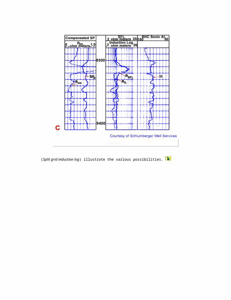
Figure 3

A 1.1 GHz electromagnetic wave is sent sequentially from each of the two transmitters, and at each of the receivers the amplitude and phase shift of the wave are measured (Figure   4) .

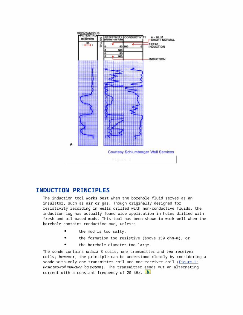
Figure 4

The absolute values of the amplitude and phase shift are found by comparison with an accurately known reference signal generated in the tool. The phase shift, the propagation time for the wave, tpl, and the attenuation A, over the receiver-receiver spacing, are calculated from the individual measurements. In each case, an average is taken of the measurements derived from the two transmitters. A complete borehole-compensated measurement is made sixty times per second; measurements are accumulated and averaged over an interval of either 2 or 6 inches of formation prior to recording on film and tape.

Due to the close proximity of the receivers to the transmitters, spherical waves are measured; therefore, a correction factor is applied to the measured attenuation so that the plane wave theory may be used. The increased attenuation due to the spherical spreading of the wave is compensated for by applying a spherical loss correction factor SL. The corrected attenuation, Ac, is given by Ac = A -SL. In air, SL has a value of about 50 db, but, because the term is porosity dependent, a more exact approach can be taken when correcting downhole measurements:

SL = 45.0 + 1.3 tpl + 0.18tpl2

The formation dielectric parameters can then be obtained from the log data, since the attenuation factor, a, is directly proportional to the recorded attenuation, A, and the phase shift, b, is proportional to the propagation time

Tpl (= tpl).

The basic data available from the EPT sensors are propagation time Tpl and attenuation, A. A separate tool section provides microlog and caliper measurements. A standard log presentation is shown in Figure   5 over an interval containing two sandstones (168-179 m and 202-207 m)

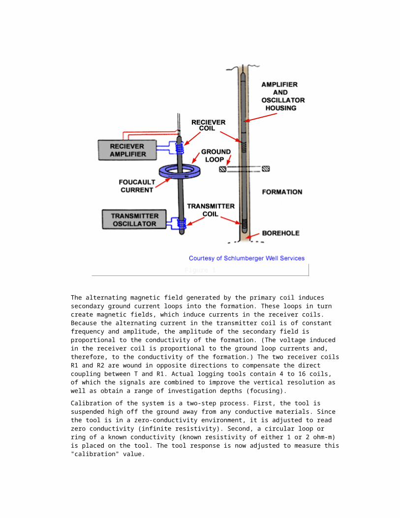
separated by shale.

Figure 5

Track 1 contains the borehole diameter (HD) and the micro-normal (MNOR). The microinverse (MINV) resistivity curves, electromagnetic wave attenuation (EATT), and propagation time (TPL) are recorded in Tracks II and III. The measurement of the smaller caliper arm (SA) can be displayed to monitor the borehole rugosity, and hence the quality of the EPT data.

INTERPRETATION METHODSThe EPT measurement responds more to the water of a formation than to the matrix or any other fluid. The water present in a formation can be the original connate water, mud filtrate, or bound water associated with shales. Because of the shallow depth of investigation of the tool (1 to 6 inches), it can usually be assumed that only the flushed zone is influencing the measurement, hence the free water is filtrate.

Under normal circumstances, if fresh muds are used, the propagation time of the electromagnetic waves is essentially unaffected by the water salinity (Figure   6).

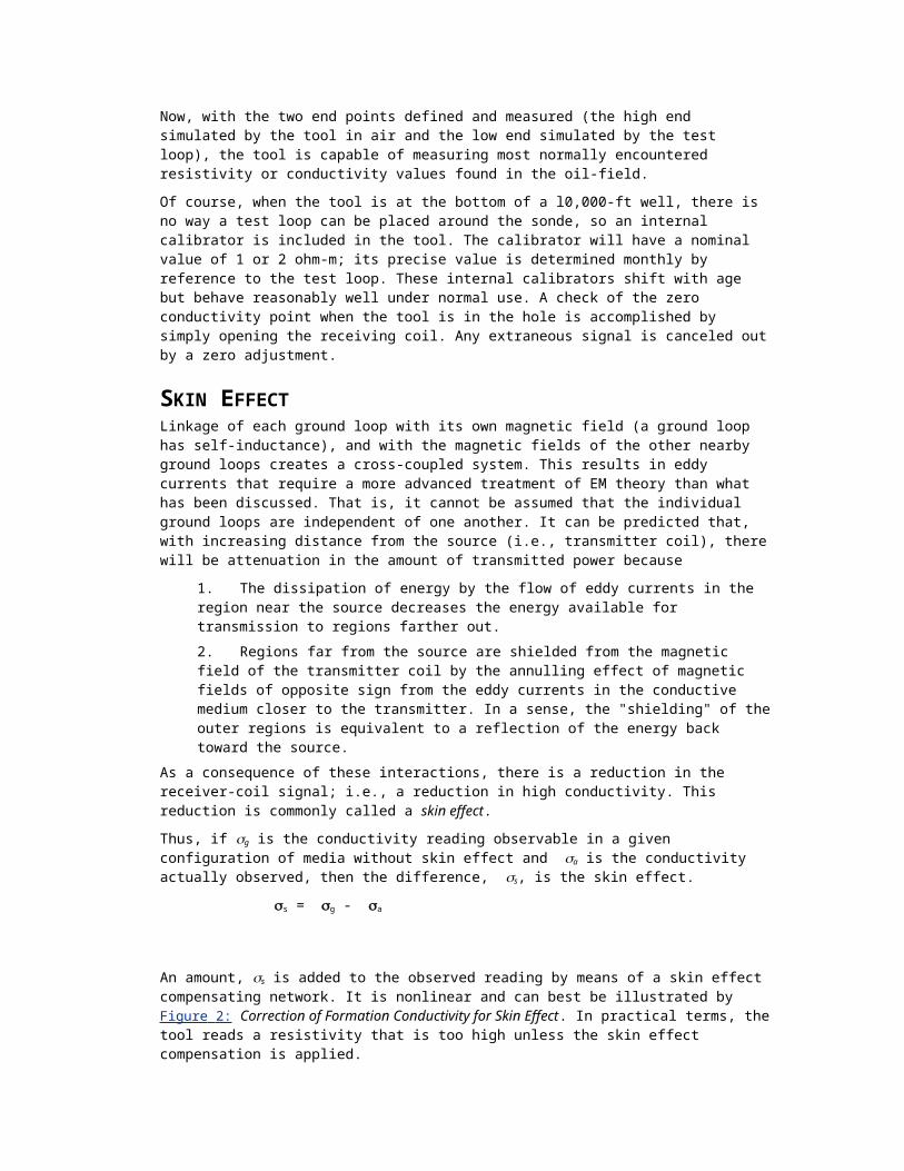
Figure 6 .

An increase in salinity increases the loss factor " and decreases the permittivity’, but the effects tend to cancel each other out. If salt-saturated fluids are encountered, the loss factor increases to the extent that the electromagnetic waves are highly attenuated, and therefore measurements are more prone to error.

The EPT measurements are unaffected by mudcake up to a thickness of about 0.4 inch, but rugosity can result in spurious readings as mud comes between the antenna pad and the formation. The situation deteriorates further in boreholes filled with air or oil, where even a thin film of the fluid results in the tool responding only to the fluid and not to the formation. The tool works well, however, in emulsion and inverse emulsion muds.

Porosity from Travel Time (TPO Method)The most-used relationship to convert travel time to porosity is a weight-average relationship similar to that used in density logging.

Travel time of microwaves in clean, porous media is given by the sum of the travel times through the component parts:

tpo2 = tpl

2 - (Ac2/3604)

tpo = tpf + (1 - ) tpm

Solving for the porosity,

= (tpo -tpm) / (tpf -tpm)

where:

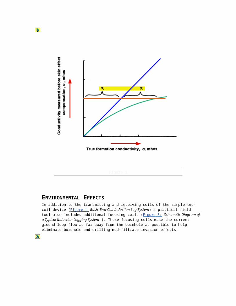
Ac = the attenuation corrected for spreading loss

tpo = the loss-free travel time of the medium, ns/m

tpl = the measured travel time of the medium, ns/m

tpm = the travel time of the rock matrix, ns/m

tpf = the travel time of the fluid in the pores, ns/m

The tpl is measured by the tool, then the following may be calculated:

tpo2 = tpl

2 - (Ac2/3604)

Once tpo is determined, the rest of the equations can be computed to obtain porosity ().

At the wellsite, a computation program computes the water volume from the EPT measurement using the tpo method and gives the amount of moved hydrocarbon.

Another method compares the EPT porosity with the total porosity measured by the neutron, density, and acoustic tools. This allows a quick-look determination of the water saturation in the flushed zone. Figure   7 is an example comparing the sonic porosity with the EPT porosity.

Figure 7

The sonic porosity (SPHI) and EPT porosity (EMCP) are displayed in Tracks II and III, and the computed gamma ray (CGR) and total gamma ray (SGR) are recorded in Track I. There is a change of lithology at 245 m, with a limestone above this depth and a sandstone with calcareous cement below. The limestone and lower section of the sandstone are water bearing, and the

hydrocarbon content of the upper section of the sand is clearly indicated by the separation of the two porosity curves. The original oil/water contact is at 267 m, while the present contact is at 261 m. Generally, the EPT porosity reads the same as a nuclear-derived porosity in water-bearing zones and shales, but in hydrocarbon-bearing intervals the EPT porosity is less than either the total porosity or the density porosity. In gas zones, the separation between the neutron porosity and the EPT porosity is not so apparent.

DIELECTRIC CONSTANT LOG (DCL)In contrast to the EPT, other dielectric logging devices (Figure   8 ) use a lower operating frequency (approximately 10 to 50 MHz) and a much longer spacing between transmitter and receiver (on the order of 3 feet).

Figure 8

Since the tool measures formation properties beyond the invaded zone, it can be used for monitoring enhanced recovery projects where plastic pipe has been set. Figure   9 shows the progress of a waterflood through repeat logs on different dates.

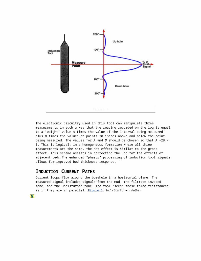
Figure 9

Density Logs

OVERVIEW OF DENSITY AND PHOTOELECTRIC LOGS

FORMATION DENSITY TOOLDensity is one of the most important pieces of data in formation evaluation. In the majority of the wells drilled, density is the primary indicator of porosity. In combination with other measurements, it may also be used to indicate lithology and formation fluid type.

A conventional compensated density log is shown in Figure   1: FDC Log Presentation,

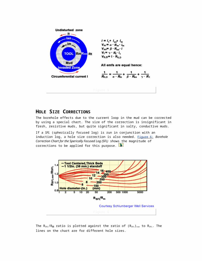
Figure 1

with the value of formation bulk density (rb) in tracks 2 and 3. The most frequently used scales are a range of 2.0 to 3.0 gm/cc or 1.95 to 2.95 gm/cc across two tracks. A correction curve, r, is sometimes displayed in track 3 and less frequently in track 2. The gamma ray and caliper curves usually appear in track 1.

The tool can be used by itself, but is typically run in combination with other tools, such as the compensated neutron and resistivity tools. The formation density skid device (Figure   2 : Schematic of the Dual-Spacing Formation Density Logging Device (FDC)) carries a gamma ray source and two detectors, referred to as the short-spacing and long-spacing detectors.

Figure 2

This tool is a contact-type tool; i.e., the skid device must ride against the side of the borehole to measure accurately.

The tool employs a radioactive source which continuously emits gamma rays. These pass through the mudcake and enter the formation, where they progressively lose energy until they are either completely absorbed by the rock matrix or they return to one the two gamma ray detectors in the tool. Dense formations absorb many gamma rays, while low-density formations absorb fewer. Thus, high-count rates at the detectors indicate low-density formations, whereas low count rates at the detectors indicate high-density formations. For example, in a thick anhydrite bed the detector count rates are very low, while in a highly washed-out zone of the hole, simulating an extremely low-density formation, the count rate at the detectors is extremely high.

Gamma rays can react with matter in three distinct manners:

Photoelectric effect, where a gamma ray collides with an electron, is absorbed, and transfers all of its energy to that electron. In this case, the electron is ejected from the atom.

Compton scattering, where a gamma ray collides with an electron orbiting some nucleus. In this case, the electron is ejected from its orbit and the incident gamma ray loses energy.

Pair production, where a gamma ray interacts with an atom to produce an electron and positron. These will later recombine to form another gamma ray.

Photoelectric interaction can be monitored to find the lithology-related parameter, Pe. For the conventional density measurement, only the Compton scattering of gamma rays is of interest.

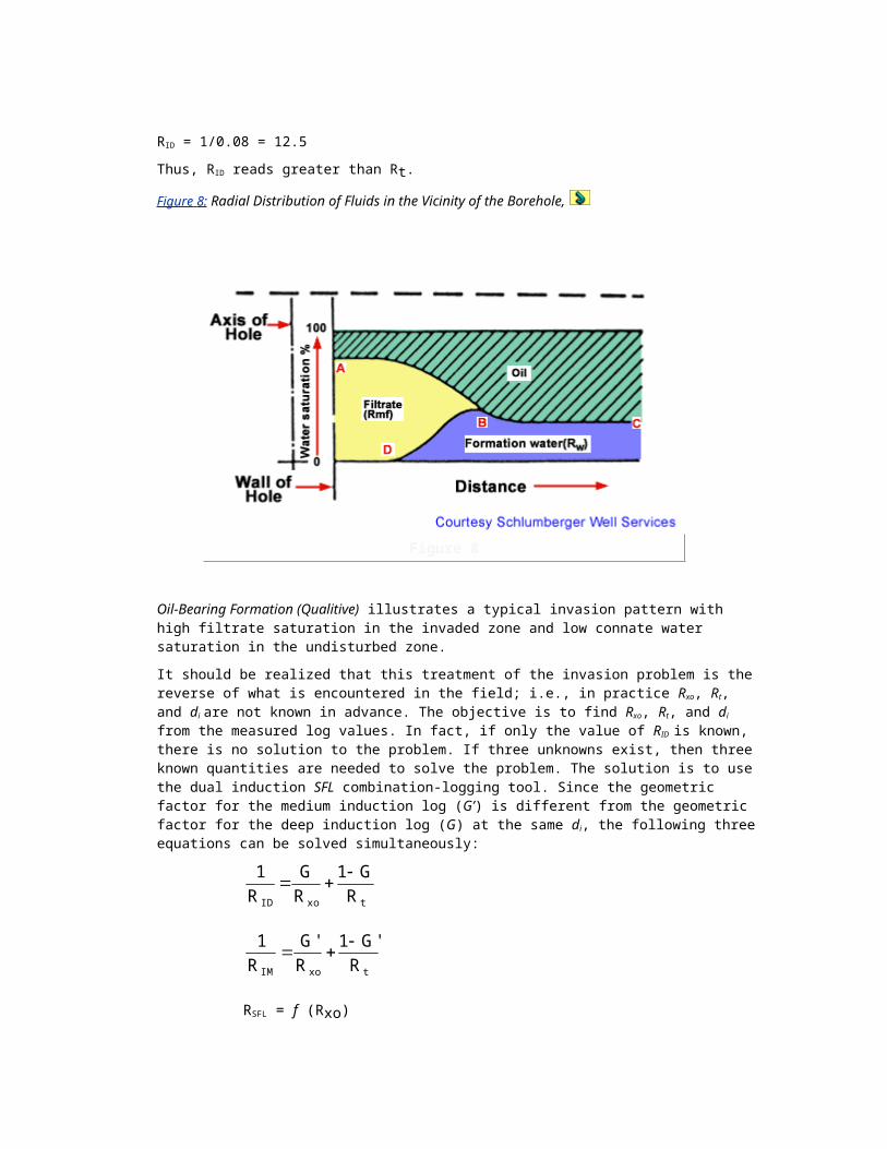
Conventional logging sources do not emit gamma rays with sufficient energies to induce pair production, therefore pair production will not be a topic of this discussion.

Since the density of a mixture of components is a linear function of the densities of its individual constituents, it is a simple matter to calculate the porosity of a porous rock. Consider the bulk volume model of a clean formation with water-filled pore space (Figure   3 : Bulk-Volume Model of Porous Rock Formation).

Figure 3

Unit volume of porous rock consists of a fraction made up of water and a fraction (1-) made up of solid rock matrix. The bulk density of the sample can be written as:

 rb = rma (1-) + rf

 where rma refers to the matrix density and rf refers to the fluid density. Simple rearrangement of the terms leads to an expression for porosity given by:

 D = (rma -rb) / (rma -rf)

 The same concept can be illustrated graphically as given in Figure   4: Density Porosity Graph,

Figure 4

where bulk density, rb is plotted against porosity, . Note that points falling on the line connecting the matrix point (rma, = 0%) and the water point (rf, = 100%) represent all possible cases extending from a zero-porosity rock matrix to 100% porosity. Any intermediate value of rb corresponds to some porosity, .

The matrix density in normal reservoir rocks varies between 2.87 gm/cc (dolomite) and 2.65 gm/cc (sandstone). The fluid density of normal brines ranges from 1 to 1.1 gm/cc and is controlled by the properties of the invading mud filtrate in permeable zones. Porosity derived from a density log is denoted as D.

The density log gives reliable porosity values, provided the borehole is smooth, the formation is shale-free, and the pore space does not contain gas. In shaly formations and/or gas-bearing zones, it is necessary to refine the interpretative model to make allowances for these additions or substitutions to the rock system.

LITHOLOGIC DENSITY TOOLThe Pe, or lithodensity log, run with the lithodensity tool (LDT), is another version of the standard formation density log. In addition to the bulk density (rb), the tool also measures the photoelectric absorption index (Pe) of the formation. This new parameter enables a lithological interpretation to be made without prior knowledge of porosity.

The photoelectric effect occurs when a gamma ray collides with an electron and is absorbed in the process, so that all of its energy is transferred to the electron. The probability of this reaction taking place depends upon the energy of the incident gamma rays and the type of atom. The photoelectric absorption index of an atom increases as its atomic number, Z, increases.

Pe = (0.1 . Zeff)3.6

The lithodensity tool is similar to a conventional density logging device, and uses a skid containing a gamma ray source and two gamma ray detectors held against the borehole wall by a spring-actuated arm (Figure   5: The Lithologic Density Tool). Gamma rays are emitted from the tool and are scattered by the formation, losing energy until they are absorbed via the photoelectric effect.

Figure 5

At a finite distance from the source, there is a gamma ray energy spectrum as shown in Figure   6: Variation in Gamma Ray Spectrum for Formations of Different Densities. This Figure also shows that an increase in the formation density results in a decrease in the number of gamma rays detected over the whole spectrum.

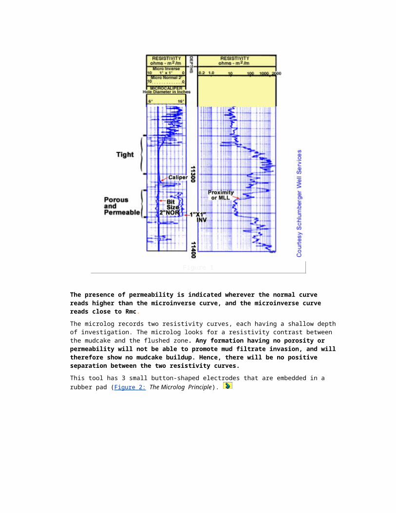
Figure 6

For formations of constant density but different photoelectric absorption coefficients, the gamma ray spectrum is only altered at lower energies, as indicated in Figure   7: Variation in Gamma Ray

Spectrum.

Figure 7

Observing the gamma ray spectrum, we notice that region H only supplies information relating to the density of the formation, whereas region L provides data relating to both the electron density and the Pe value. By comparing the counts in the energy windows H and L, the Pe can be

measured. The gamma ray spectrum at the short spacing detector is only analyzed for a density measurement, which is used to correct the formation density determined from the long spacing spectrum for effects of mud-cake and rugosity.

The photoelectric absorption coefficient is virtually independent of porosity, there being only a slight decrease in the coefficient as the porosity increases. Similarly, the fluid content of the formation has little effect. Simple lithologies, such as pure sandstone and anhydrite, can be read directly from logs using Pe curves. Look for the following readings in the most commonly occurring reservoir rocks and evaporites.

Material

 

Pe

 Sand

 

1.81

 Shale

 

3-4

 Limestone

 

5.08

 Dolomite 3.14

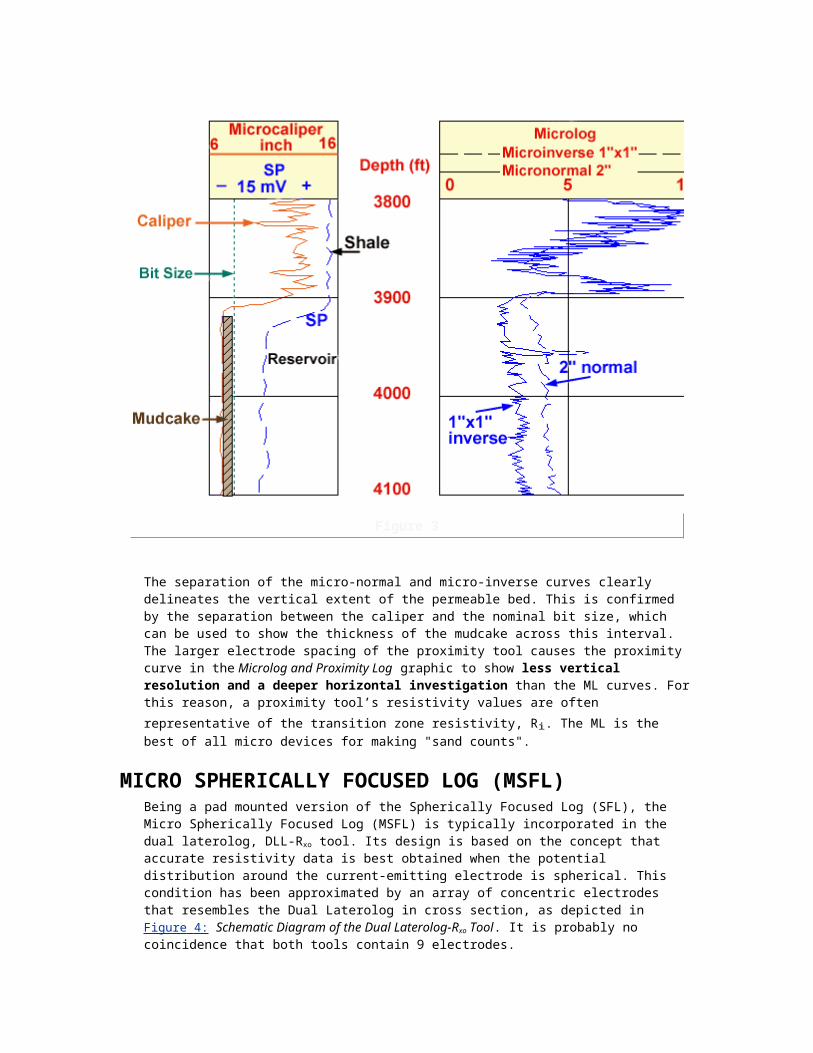
   Salt

 

4.65

 Anhydrite

 

5.05

 

PRINCIPLES OF DENSITY LOGGINGIn contrast to the natural gamma-ray tool, which only contains a passive detector, the density tool contains a chemical gamma-ray source (Cesium 137 or Cobalt 60), and two or more gamma-ray detectors. The density tool is therefore called an induced gamma or gamma-gamma tool. The induced gamma-rays are scattered by the rock and only a few reach one of the gamma-ray detectors in the tool (Figure   1, Dual-Spacing Formation Density Log).

Figure 1

The denser the rock material the more the gamma-rays will be attenuated and hence fewer will reach the detectors. The use of the gamma-gamma tool for density measurements is based on this attenuation phenomenon.

INTERACTIONS BETWEEN GAMMA-RAYS AND ATOMSAs mentioned previously, there are 3 ways for an atom to interact with gamma-rays as depicted in Figure   2: Various Interactions Between Gamma Rays and the Si Atom.

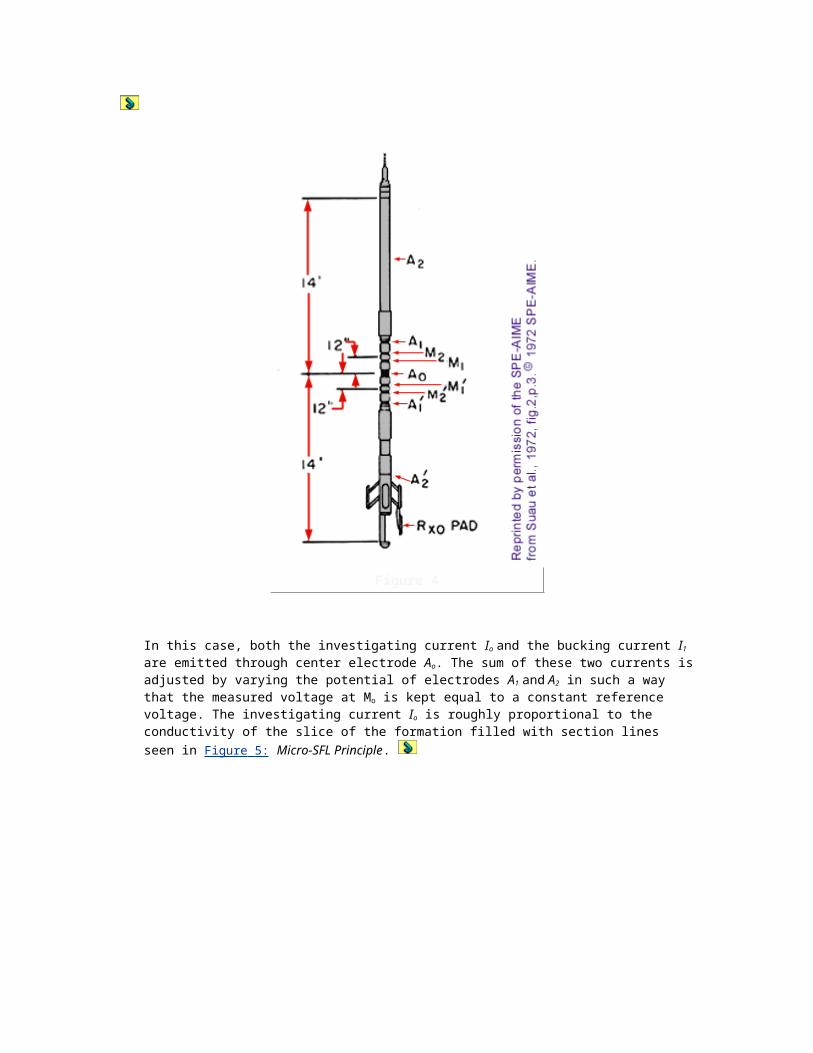
Figure 2

COMPTON SCATTERING High energy gamma-rays emitted by a radioactive source collide with the electrons in the formation. At each collision, the photon loses some of its energy to an electron, which can be ejected from its orbit. The scattered gamma-ray has less energy than the gamma-ray that caused the collision, and the energy level of the scattered gamma-ray is strongly dependent on the collision angle. When the number of gamma-rays are recorded as a function of their energy in a frequency vs. energy diagram, an energy spectrum may be obtained. The energy spectrum of the scattered gamma’s is the well known Compton continuum.

PHOTOELECTRIC EFFECTAfter several collisions the gamma-rays that result have low energies (< 0.5 MeV). Below this energy level the photoelectric effect becomes predominant. The gamma-rays can then interact with the electrons of the inner bands. The gamma energy is used to push an electron into a higher band. If the electron falls back to the original band, gamma-rays are emitted with energies characteristic for the atomic number.

PAIR PRODUCTIONIn this process, the high energy photon (>2 MeV) looses all it's energy and the gamma-ray is converted into an electron and a positron. The positron combines almost immediately with another electron, and two gamma-rays (each with an energy of 1.04 MeV) are emitted in opposite directions.

Figure   3 : Gamma Ray Mass Absorption Coefficient illustrates the concept of the mass absorption

coefficient.

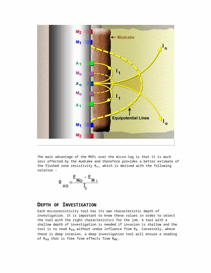
Figure 3

When an incident beam of gamma rays with initial intensity Iin strikes a target of thickness x, then its intensity is reduced on passing through the target in such a way that:

Iout = Iin e-µx

where Iout is the resulting intensity of the beam at the other side of the target, and µ is the mass absorption coefficient. This coefficient µ is a function of both the type of material in the target and the type of interaction that takes place.

Or, stated differently,

ln (Iout/Iin) = -. x

In other words, the logarithm of the ratio of intensities of the attenuated and the original beams is proportional to the target thickness and a proportionality factor , which is defined as the mass absorption coefficient.

In Figure   4: Gamma Ray Mass Absorption Coefficient Over the Energy Range of Interest the

mass absorption coefficient expressed in cm2/g, is plotted the energy of the gamma rays.

Figure 4

The lines indicate the probability that one of the three interactions described above will occur as a function of the gamma-ray energy. Conventional gamma ray sources in logging tools are made of cesium, and the emitted gamma rays have an energy of 0.661 MeV, so from this graphic, we can see that it is highly unlikely that any form of pair production will occur, since this type of interaction only occurs at energies higher than 2 or 3 MeV. The detectors used in conventional density tools have a practical lower limit to the gamma ray energy level that they can detect. This lower limit is about 0.2 MeV. Thus, the operating range shown in the graphic is between the two vertical lines marking the energy range between the gamma rays emitted from the source and the limit of detection by the detectors. Compton scattering therefore becomes the most probable form of interaction that conventional density tools can monitor. For this reason, pair production does not need to be considered in the context of gamma-gamma logging.

DENSITY TOOL CONFIGURATIONIn order to minimize the influence of the mud column the tool features two or more gamma-ray detectors. The configuration with two detectors at approximately 8 and 16 inches from the source is shown in Figure   5: Schematic of the Dual-Spacing Formation Density Logging Device (FDC).

Figure 5

Both the detectors and the source are mounted on a skid and shielded from the borehole. The skid, which has a plow-shaped leading edge to remove part of the mudcake, is pressed firmly against the wall by means of an eccentering arm. The two detectors are necessary to account for remaining mudcake or mud interposed between the skid and the formation. The litho-density tool (LDT) offers a combination of the density and photo-electric absorption Pe measurements.

The net effect of gamma ray Compton scattering and absorption is that the count rate seen at the detector is logarithmically proportional to the formation density (Figure   6: Detector Count Rates vs. Formation Density Measurements):

Figure 6

log (count rate) = A + B • (formation density)

Both near-and far-spacing detectors behave in this way, so that a plot of far versus near count rates also produces a straight line (Figure   7: Near and Far Count Rates of the Formation Density Tool). Note that formation density increases as count rates decrease.

Figure 7

ADVERSE INFLUENCES AND CALIBRATION

MUDCAKE COMPENSATIONAlthough the source and detectors are pressed against the borehole wall, there will inevitably be small wash-outs and irregularities (collectively termed borehole rugosity) that will attenuate the gamma-ray reading. Moreover, there is often a thin layer of mudcake between the skid and the borehole wall. A mudcake with a density that is different from formation density will change both the near-and far-count rates.

The two detectors have a different depth of investigation because of their short (SS) and long (LS) spacing from the source (Figure   1 : Schematic of the Dual-Spacing Formation Density Logging

Device).

Figure 1

The rugosity and mudcake each produce a different effect on the SS and LS detector responses. By combining the responses of the two detectors, the effect of the mudcake and small wash-outs can be compensated.

Figure   2: Mudcake Compensation shows where a plotted point falls if a formation with a bulk density of 2.7 gm/cc has an ever-increasing amount of mudcake of density 1.5 gm/cc placed

between it and the tool.

Figure 2

In an extreme case of "infinite" mudcake thickness, both detectors would "see" only mudcake and read a value of 1.5 gm/cc.

This method is referred to as the "spine-and ribs correction". The arc describing the locus of the points is referred to as a rib; the zero mudcake line is referred to as a spine. A complete set of spine and ribs can be drawn fore various thicknesses and densities of mudcakes (Figure   3: Spine and Ribs Plot, Showing Response of Count Rates to Mudcake). Note that ribs also extend to the left of the spine for mudcakes having a density greater than the formation density; e.g., in barite muds.

Figure 3

The surface equipment associated with the density tool computes the position of the point on the spine and ribs chart, then moves the point along the rib to intercept the spine. At this point, a corrected value of r is recorded for the log. The value of r is calculated as the difference between r from the long spacing and rcor. Thus, r is positive in light muds and negative in heavy muds.

ELECTRON DENSITYSince Compton scattering is an interaction between gamma rays and electrons, the density measurement recorded by this logging tool is actually the electron density, re, not the bulk density, rb. Due to the fact that re is not exactly equal to rb for all elements, a special calibration makes the tool read correctly in fresh-water-filled limestone.

As a result of the calibration technique used, not all substances commonly found in rock formations are read correctly by the density tool. The table below lists density properties of various compounds frequently found in subsurface formations.

Table 1: The 2 Z/A Values for Various Elements

Element

 

A

 

Z

 

2 Z/A

 H

 

1.008

 

1

 

1.9841

 C 12.011 6 .9991

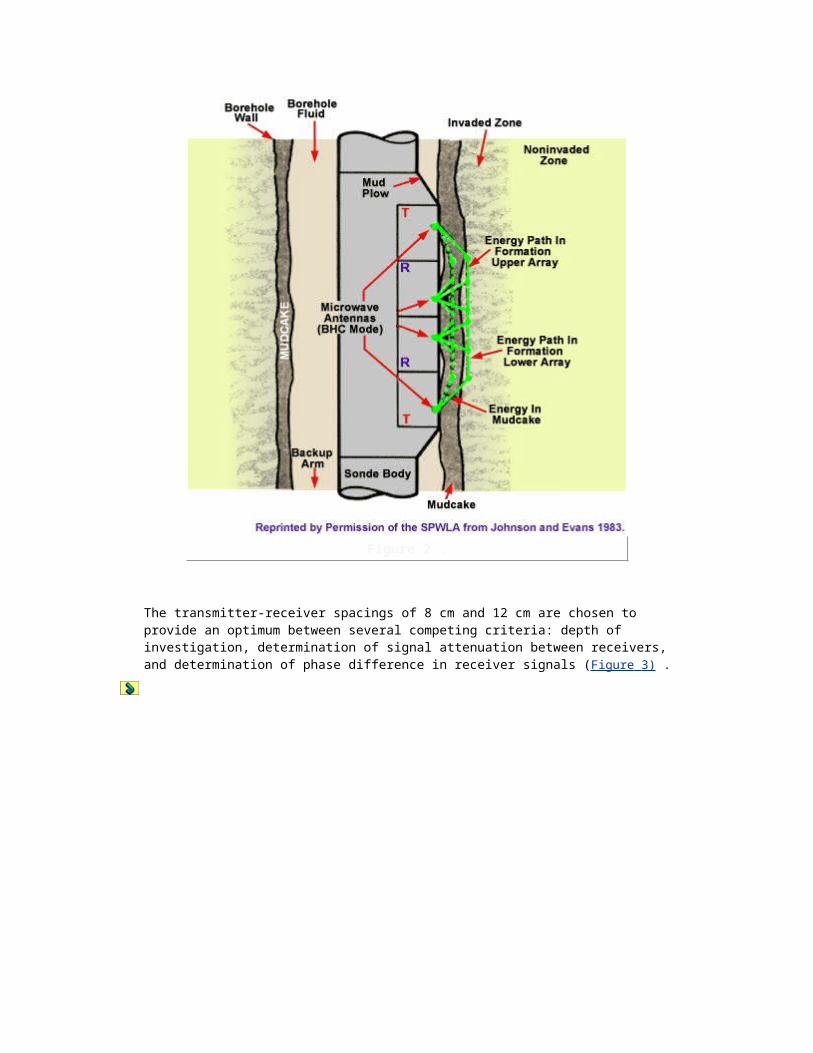
       O

 

16.000

 

8

 

1.0000

 Na

 

22.99

 

11

 

.9569

 Mg

 

24.32

 

12

 

.9868

 Al

 

26.98

 

13

 

.9637

 Si

 

28.09

 

14

 

.9968

 S

 

32.07

 

16

 

.9978

 Cl

 

35.46

 

17

 

.9588

 K

 

39.10

 

19

 

.9719

 Ca

 

40.08

 

20

 

.9980

 

CALIBRATION AND QUALITY CONTROLStandard calibrations of the density tool are made to ensure that density measurements will be consistent from one tool to the next. The primary standard is made by using man-made, laboratory formations, such as the API test pit. Sometimes, these test pits are reproduced at select service company locations. Since these cannot be transported, a set of secondary standards is available at logging service company bases in the form of aluminum, magnesium, and/or sulfur blocks of accurately known density and geometry. These blocks, which weigh up to 400 pounds, are not easily transportable though. So a field calibrator containing two small gamma ray sources is used to reproduce the same count rates as those found in the blocks.

The wellsite calibration should be performed before and after each log is run; the shop calibration should be carried out at least every 60 days, and a copy of it should be attached to the main log. It is important to note that the field calibrator, the skid with the detectors, and the source all form a matched set. This means that if any of the three do not match the serial numbers on the master calibration, then the log should be rejected.

Natural benchmarks for checking the validity of a density log are salt, which has a ra of 2.032 gm/cc, and anhydrite, which has a ra of 2.977 gm/cc. These minerals may not appear in the wellbore being logged; and even if they do, they may not be 100% pure, and should be used with caution. In general, density logs are either well calibrated (and therefore correct) or they are very noticeably bad.

Apart from the natural benchmarks already discussed, the next best quality check is a review of the r curve. If the short-spacing detector fails, then the whole compensation mechanism is thrown out of kilter. If r is roughly within the limits of ± 0.05 gm/cc, then the log may be assumed to be correct. If r is negative in light muds, something is wrong. Likewise, positive values of r in heavy (barite) muds would also be a danger signal.

APPLICATIONS The Formation Density log has a number of applications:

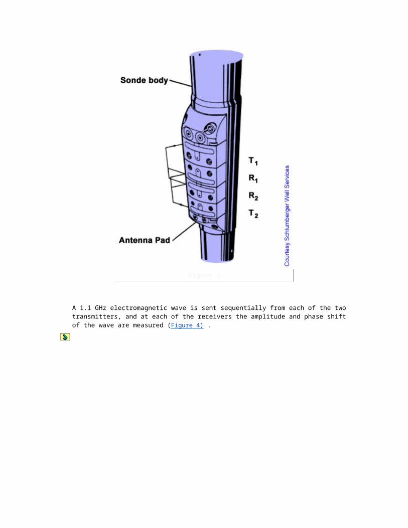
Measuring density of the formation

Calculation of porosity

When combined with sonic travel times, the density data gives the acoustic impedance, which is important for calibration of seismic data

Identification of evaporites

Gas detection in reservoirs when used in combination with the neutron log

The Pe curve is a good lithology indicator. The influence of reservoir porosity and fluid content (including gas) on the Pe is minor.

DENSITY OF THE RESERVOIRAt the distance of some 20 -30 cm between source and detector, the gamma-rays usually scatter two to three times before some of them reach the detector. The number of collisions between the electrons and gamma’s is directly related to the number of electrons in the formation. A low count is indicative of a high number of electrons and thus for a high density formation. The response of the density tool is essentially determined by the electron densityre that is related to

the bulk density, rb as follows:

  A

ZN be

rr

 where

       

 

re

 

=

 

electron density (number per volume unit)

 

 

N

 

=

 

Avogadro's number (6.03 x 1023 atoms per gram-atom)

 

 

Z

 

=

 

atomic number (number of protons) (d.I.)

 

 

rb

 

=

 

bulk density, (gr/cc)

 

 

A

 

=

 

atomic weight, related to number of protons + neutrons

 The bulk density depends on the density of the rock material, its porosity, and the densities of the different phases of fluids (oil / gas / water) that are present in the pore space. For most formation substances, the factor 2 Z/A) is very close to unity (for hydrogen close to 2), as demonstrated below, in Table 1.

Table 1: The 2 Z/A Values for Various Elements

Element

 

A

 

Z

 

2 Z/A

 H

 

1.008

 

1

 

1.9841

 C

 

12.011

 

6

 

.9991

 O 16.000 8 1.0000

   

 

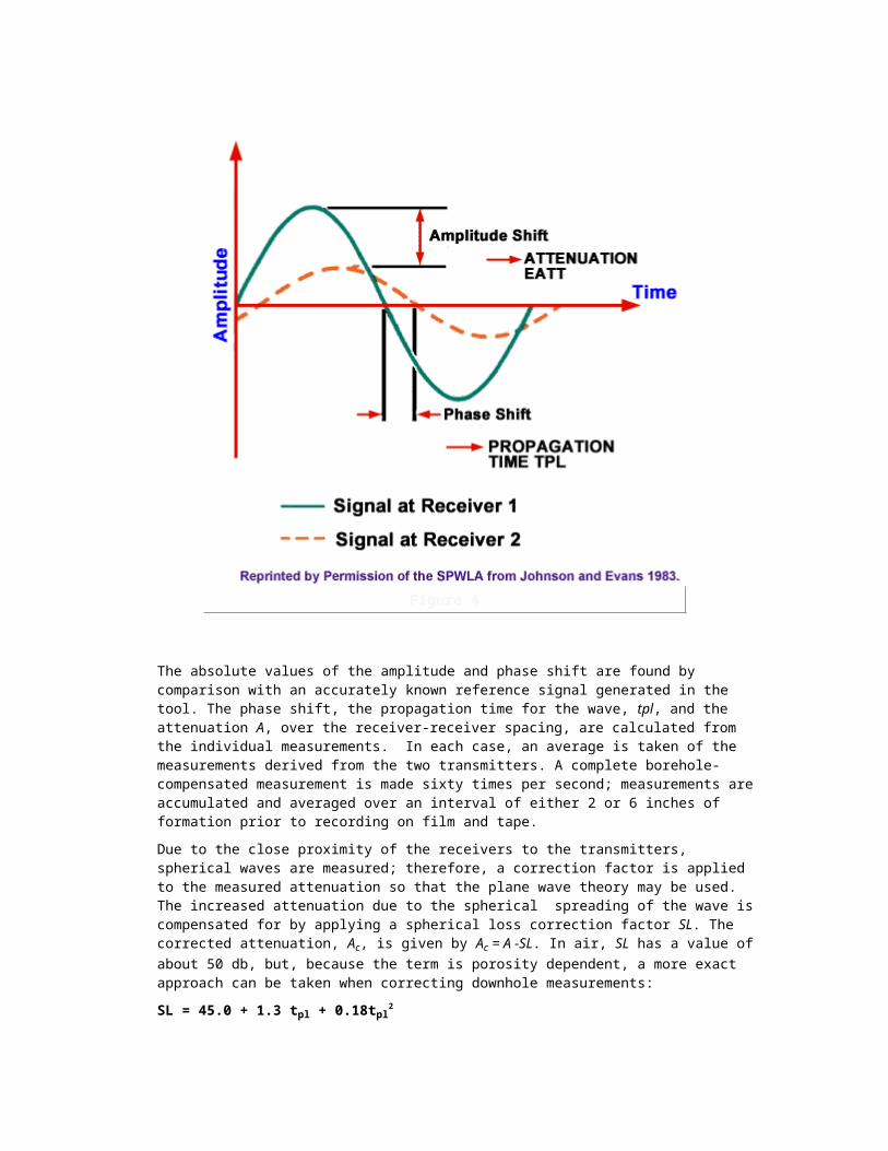
 Na

 

22.99

 

11

 

.9569

 Mg

 

24.32

 

12

 

.9868

 Al

 

26.98

 

13

 

.9637

 Si

 

28.09

 

14

 

.9968

 S

 

32.07

 

16

 

.9978

 Cl

 

35.46

 

17

 

.9588

 K

 

39.10

 

19

 

.9719

 Ca

 

40.08

 

20

 

.9980

 The resulting apparent bulk density ra, as seen by the tool, is related to the electron density re:

 188.007.1 ea rr

 For liquid filled sandstone, limestone and dolomite the tool reading ra is practically identical to the

actual density rb, as shown in the table below.

Table 2: Values Related to the Density Tool.

Name of Compound

 

Formula for Compound

 

Actual Densi

ty rb

 

2SUM(Z's) /mol.weight

 

Electron

Density re

 

Apparent Density

(tool) ra

 

Quartz

 

SiO2

 

2.654

 

0.9985

 

2.650

 

2.648

 Calcite

 

CaCo3

 

2.710

 

0.9991

 

2.708

 

2.710

 Dolomite

 

CaCO3MgCO

3

 

2.870

 

0.9977

 

2.863

 

2.876

 

Anhydrite

 

CaSO4

 

2.960

 

0.9990

 

2.957

 

2.977

 

Anth. coal

  1.4-1.8

1.030 1.442-1.852

1.355-1.796

         Bitum. coal

 

  1.2-1.5

 

1.060

 

1.272-1.590

 

1.173-1.514

 

Fresh water

 

H2O

 

1.000

 

1.1101

 

1.110

 

1.00

 

Salt water

 

200.000 ppm

 

1.146

 

1.0797

 

1.237

 

1.135

 

"Oil"

 

n(CH2)

 

0.850

 

1.1407

 

0.970

 

0.850

 Methane

 

CH4

 

rmeth

 

1.247

 

1.247rmet

h

 

1.335rmeth-0.188

 "Gas"

 

C1.1H4.2

 

rg

 

1.238

 

1.238rg

 

1.325rg-

0.188

 Corrections are required in anhydrite, sylvite, halite and also in gas bearing formations. For a number of minerals the characteristics are given in Table 2, in which rmeth , and rg are the

density of methane and composite gas respectively.

DENSITY-POROSITY OF THE RESERVOIRFor a clean formation of matrix density rma containing a fluid with density rfl, the bulk densityrb as measured by the log can be expressed as a linear relationship between matrix and fluid points.

 flmab )1( rrr

rearranged :

flma

bma

rrrr

 

When the pores contain a mixture of mudfiltrate and hydrocarbons, rfl is calculated as follows:

 hcxomfxofl )S-(1+S rrr

 where

       

 

rb

 

=

 

bulk density, g/cc

  = porosity in fraction of bulk volume

       

 

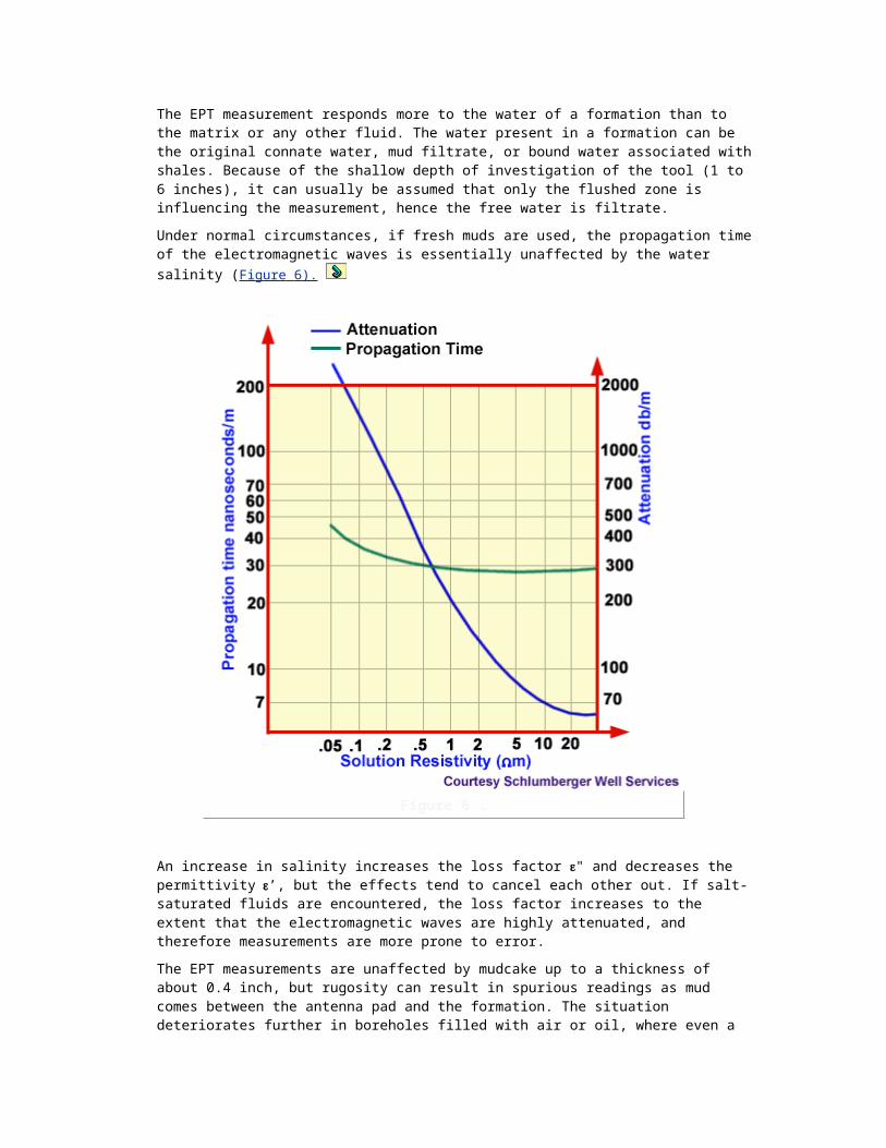
rma

 

=

 

matrix density, g/cc

 

 

rfl

 

=

 

fluid density, g/cc

 

 

rhc

 

=

 

hydrocarbon density, g/cc

 

 

rmf

 

=

 

mudfiltrate density, g/cc

 

 

Sxo

 

=

 

mudfiltrate saturation in fraction of pore volume

            The volume fraction of mudfiltrate in the pore space in the flushed zone is usually much larger than that of the hydrocarbons. The hydrocarbon effect is therefore usually small, unless light oil or gas is present. In Figure   1:

Figure 1

Core Porosity versus rb the core porosity is plotted versus the bulk density. Extrapolation of the

regression line to the point where it intersects the density axis provides the apparent matrix value, rma.

Pe RESPONSE AND DETERMINATION OF FORMATION LITHOLOGY

The photoelectric effect, Pe curve is an index of the effective photoelectric absorption cross section

of the formation. The unit of the photoelectric absorption cross section is in barns (10-24 cm2) per

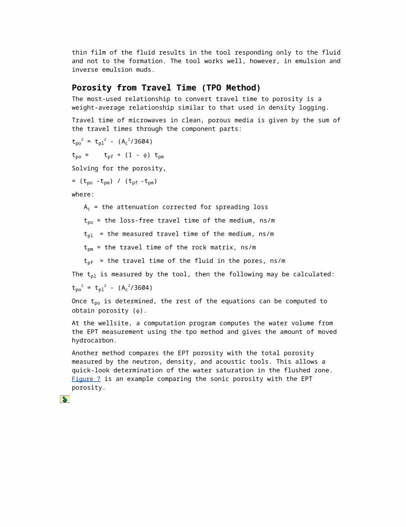
atom. As previously mentioned, the gamma rays of the photoelectric effect are produced when electrons in the inner bands return to their original state. The energy of these gamma rays is therefore dependent on the binding forces of electrons in the inner bands and strongly dependent on the atomic number Z:

[E-1]  4.6ZK=

 where

       

 

 

=

 

photoelectric absorption cross section in barns per atom

 

 

Z

 

=

 

atomic number

 

 

K

 

=

 

constant

 The coefficient K varies with the energy level of the incident gamma rays. Dividing by Z and calibrating the Pe log such that K is arbitrarily taken to be E-3.6, yields:

[E-2] 

3.6e Z/10)(P

 

where Pe is again the effective photoelectric absorption cross section, but now expressed in barns/electron. To obtain a parameter that is proportional with the volume fractions of the formation constituents Pe is multiplied with the electron density. This yields the effective photoelectric absorption cross section index per unit volume U=Pe.re .The formation can then be described by the relative volumes of the components:

[E-3]

  mafl U)1(U=U  

The effective photoelectric absorption cross section per unit volume U is, as demonstrated by equations [E-2] & [E-3], strongly dependent on the atomic number and therefore an excellent lithology indicator.

Neutron Logs

INTRODUCTION TO NEUTRON LOGGINGNeutron tools were the first logging instruments to use radioactive sources for determining the porosity of the formation. After the later introduction of the gamma-gamma density tool, the neutron measurement was applied in conjunction with the density porosity reading in order to recognize and correct for effects of shale and gas.

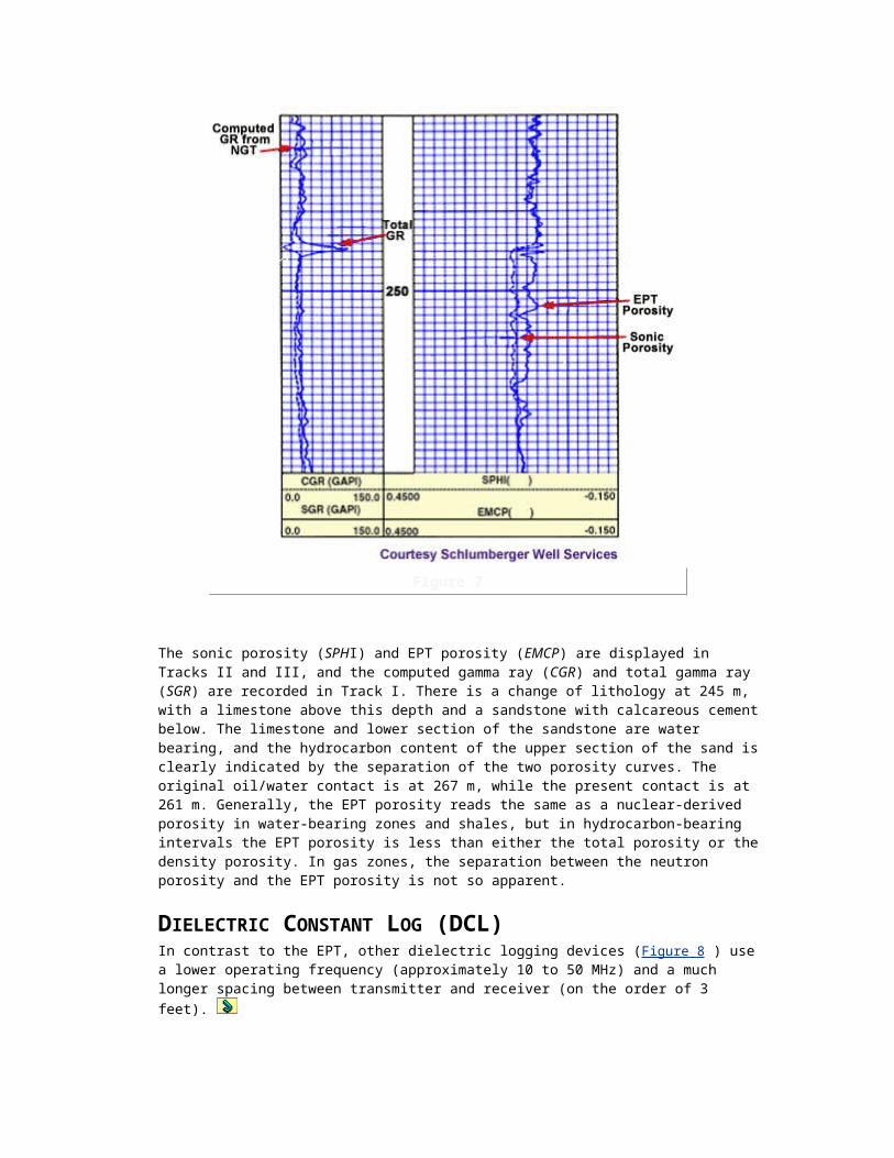
Neutron tool response is dominated by the concentration of hydrogen atoms in the formation. In clean reservoirs containing little or no shale, the neutron log response will provide a good measure of formation porosity if liquid-filled pore spaces contain hydrogen, as is the case when pores are filled with oil or water (hydrogen index =1, see Hydrogen Index below). By contrast, when logging shaly or gas-bearing formations, a combination of Neutron and Density readings will often be required for accurate porosity assessment.

NEUTRON LOGGING APPLICATIONSNeutron tools are used primarily to determine:

porosity, usually in combination with the density tool

gas detection, usually in combination with the density tool, but also with a sonic tool

shale volume determination, in combination with the density tool

lithology indication, again in combination with the density log and/or sonic log

formation fluid type.

Depending on the device, these applications may be made in either open or cased holes. Additionally, because neutrons are able to penetrate steel casing and cement, these logs can be used for depth tie-in as well as providing information on porosity and hydrocarbon saturations in cased holes. Figure   1: Generalized Neutron Logging Tool illustrates a typical neutron logging tool.

Figure 1

BASIC PRINCIPLESThe electrically neutral neutron has a mass that is practically identical to that of the hydrogen atom. The neutrons that are emitted from a neutron source have a high energy of several million electron volts (MeV). After emission, they collide with the nuclei within the borehole fluid and

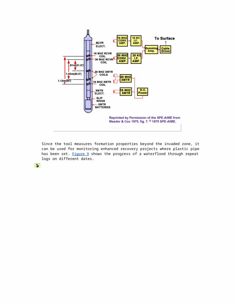
formation materials. With each collision, the neutrons loose some of their energy (Figure   2:

Emission, Traveling and Collisions of a Neutron in a Formation).

Figure 2

The largest loss of energy occurs when the neutrons collide with hydrogen atoms. The rate at which the neutrons slow-down depends largely on the amount of hydrogen in the formation.

With each collision the neutrons slow down, until the neutrons reach a lower (epithermal) energy state and then continue to lose energy until they reach an even lower (thermal) energy state of about 0.025 eV. At this energy the neutrons are in thermal equilibrium with other nuclei in the formation. At thermal speeds, the neutrons will eventually be captured by a nucleus. When a nucleus captures a thermal neutron, a gamma ray (called a gamma ray of capture)is emitted to dissipate excess energy within the atom.

The amount of energy lost at each collision depends on the relative mass of the target nucleus, and the scattering cross section. (At the nuclear level, the term cross section is defined as the effective area within which a neutron must pass in order to interact with an atomic nucleus. Such interactions are typically classified either as neutron capture or as neutron scatter. The cross-section is a probabilistic value dependent on the nature and energy of the particle, as well as the nature of the capturing or scattering nucleus.) Figure   3 (Slowing Down Power of H, O, Si for Different Neutron Energies) and Figure   4 (Neutron Energy Level versus Time After Leaving the Source) illustrate the slow-down process. Depending on the type of tool being used, either the gamma rays emitted after neutron capture, the epithermal neutrons or the thermal neutrons will be counted.

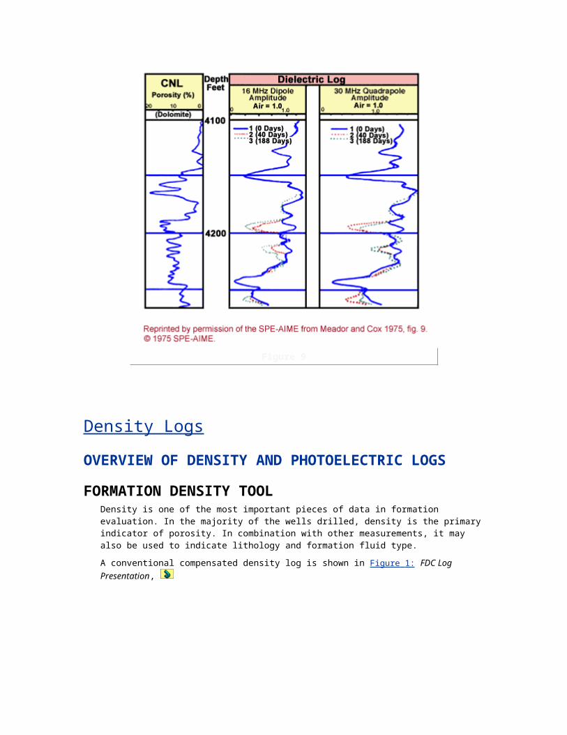
Figure 3

Figure 4

The principles of neutron logging are summarized below:

A neutron source emits a continuous flux of high-energy neutrons.

Collisions with formation nuclei reduce the neutron energy -thereby slowing it down.

At thermal energy levels (approximately 0.025 eV), neutrons are captured.

Neutron capture results in an emission of gamma rays.

Depending on the type of tool, the detector measures the slowed down neutrons and/or emitted gamma rays.

Neutron logging devices contain one or more detectors and a neutron source that continuously emits energetic (fast) neutrons.

Porosity (or the hydrogen index) can be determined by measuring epithermal or thermal neutron populations, or by measuring capture gamma rays, or any combination thereof.

Neutron logs that detect epithermal neutrons are referred to as sidewall neutron logs. By contrast, the compensated neutron log, in widespread use today, detects thermal neutrons, using two neutron detectors to reduce borehole effects. Single thermal neutron detector tools, of poorer quality, are also available in many areas of the world.

Capture gamma rays are used for porosity determination, and logs of this type are referred to as neutron-gamma logs. The responses of these devices are dependent upon such variables as porosity, lithology, hole size, hole rugosity, fluid type, and temperature.

Compensated and sidewall logs use corrections from their electronic panels to account for some of these variables, while neutron-gamma logs require departure curves (provided in chartbooks) to make corrections.

Hydrogen IndexHydrogen concentration may be defined in terms of the Hydrogen Index (HI), which is proportional to the quantity of H atoms per unit volume. The hydrogen index of fresh water at surface conditions is taken as unity.

  O)H cc 1in atoms H of(number ) (volume

atoms H ofnumber =HI

2 

For a paraffinitic oil (nCH2) we find HIoil = 1.29.roil. If the in-situ density of this oil is 0.78 g/cc, its

hydrogen index is equal to that of water, which by definition has a value of 1.

For methane (CH4), the hydrogen index depends strongly on the gas pressure. A typical value for

HICH4 is 0.225 at 100 bar.

Since the zone of investigation of the neutron tool is often confined to the flushed zone, the porosity derived from the neutron log, n is related to the true porosity, by the equation:

 ))S1(HI+SHI(

xohcxomfn

 In the above quoted case of paraffinitic oil with a density of 0.78 g/cc density, we find n = .

In the case of CH4 with in-situ density 0.1 g/cc and a flushed zone water saturation Sxo of 0.7 we find:

  0.77=0.3) 0.225+0.71(

n

 

NEUTRON POROSITY MEASUREMENTSConventional neutron porosity tools use a radioactive source to emit neutrons that have an average energy of 4.5 million electron volts (MeV). The tool’s neutron detector will detect some of these neutrons after they lose energy through elastic collisions with nuclei in the formation. But the neutron detector only comes into play toward the end of a complex chain involving neutron scatter and capture. The ability of a nucleus to slow down or capture a neutron is measured by its cross section. Cross sections for slowing down or capturing neutrons vary with different elements and with neutron energy.

Two elements, hydrogen and chlorine, dominate the behavior of all neutron tools. Hydrogen, being the element with a single proton for a nucleus, provides the best material for slowing down a neutron. Simple mechanics reveal that when two balls collide, the maximum energy loss occurs when the two balls are of equal mass. Thus, the equal mass of hydrogen’s neutron and proton account for its prodigious power to slow down neutrons.

Generally, the count rate at a neutron detector is inversely proportional to the amount of hydrogen in the formation. When the hydrogen content is high, many neutrons will be slowed and captured; therefore, the count rate will be low and porosity will be high. When hydrogen content is low, fewer neutrons are absorbed in the formation, and thus more neutrons are free to reach the detector. With more neutrons reaching the detector, the count rate will be high so porosity will be low.

Chlorine has a large capture cross-section for thermal neutrons, absorbing them a hundred times faster than most other elements. After accounting for the relative abundance of all the elements and their slowing down cross sections and capture cross sections, it transpires that a neutron need collide with a hydrogen nucleus an average of 18 times to reach thermal energy. Once a neutron does reach thermal energy, it is very likely to be absorbed by a chlorine nucleus.

This explains why the original GNT tools had such a dependence on fluid salinity. A few parts per million of sodium chloride in the mud or formation water could alter their response dramatically. It also explains why the SNP was such an improvement over GNT. The tool was completely blind to capture gamma rays, since it only detected epithermal neutrons. The CNL tools theoretically are just as blind to salinity effects, since they, too, ignore the capture gamma rays from chlorine. However, small additions of boron or cadmium in the formation can seriously affect the distribution of thermal neutrons.

Conventional neutron porosity devices measure the ratio of neutrons counted by two detectors that are spaced at different distances from the neutron source. One detector is spaced closer to the source than the other, hence the two are designated as the near and far detectors. This ratio of neutron counts between the near and far detectors is less sensitive to environmental effects than the count rate from a single detector. The ratio of neutron counts is then converted to porosity units using laboratory calibrations. On most logs, the porosity measurement is expressed in terms of porosity units (p.u.) for a limestone matrix.

Interpretation can be complicated by three factors which cause the log either to read too high or too low:

Formation atom density -The formation atom density is related to the matrix density of the formation. An increase in formation atom density will increase neutron scattering, which reduces the number of neutrons that reach the detector. This, in turn, results in an increase in measured porosity.

Clays -The additional hydrogen content of hydroxyls in clays will increase the apparent porosity.

(The combined porosity increase caused by the two factors above is called the shale effect.)

Gas -The gas or excavation effect reduces porosity readings. It occurs when pore space contains gas, which contributes far less hydrogen to scatter neutrons than does water. Consequently, the count rate is higher and measured porosity is lower.

NEUTRON DETECTORSThere are two types of neutron porosity detectors, named for the energy levels of the neutrons they detect.

An epithermal detector counts neutrons with energies from a few tenths of an eV to approximately 10 eV;

A thermal detector counts neutrons with energies around 0.025 eV.

There are trade-offs involving each detector. Thermal neutron detectors have higher count rates and better counting statistics than epithermal detectors. However, elements in the formation such as chlorine or boron can capture thermal neutrons and thus lower neutron count rates, causing inflated porosity readings. Epithermal neutrons, on the other hand, will not be captured, so epithermal porosity sondes provide truer readings. The challenge for epithermal neutron porosity tools has been to develop a source that produces enough high-energy neutrons to ensure statistically meaningful count rates.

NEUTRON SOURCESTwo categories of neutron sources are found in the logging industry: chemical sources and pulsed sources.

CHEMICAL NEUTRON SOURCESGenerally speaking, chemical sources are composed of two elements in intimate contact, which react together to continuously emit neutrons. Such sources must be heavily shielded when not in use.

Chemical neutron sources usually consist of a mixture of beryllium (Be) and an alpha-emitting radioactive element (Ra, Pu, or Am). This is described by the following reaction mechanisms:

 88Ra226 ---> 86Rn222 + 2He4

 The alpha particles (He) bombards the beryllium target and both neutrons and gamma rays are produced:

 4Be9 + 2He4 ---> 6C12 + on1 + gamma rays 

Within a few microseconds, the neutrons are slowed down to the thermal energy level, as depicted in Figure   1: Neutron Energy Level versus Time After Leaving the Source.

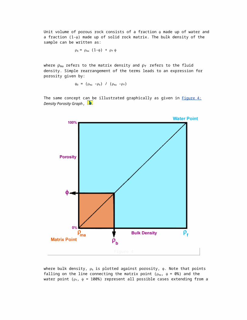
Figure 1

After slowing to the thermal energy level, they are usually captured by a Hydrogen or Chlorine nuclei in a process that can take up to 1000 s. The capturing nucleus becomes excited and emits gamma rays, e.g.:

 1H1 + 0n1 ---> 1H2 + gamma rays 

Neutron tools are configured with a detector located at distances below 1 and 2 feet from the source. The detector distances in the neutron tools (with the exception of the APS) are spaced so that the neutron density around the detector is low when the hydrogen content of the formation is high. In other words, the hydrogen atoms in the formation act as a shield to keep the neutrons away from the detectors.

The count rate of neutrons or gamma rays produced by thermal neutron capture is therefore low in formations of high porosity that contain oil or water. When dealing with a low porous rock, the neutrons can penetrate further, so the count rate around the detector will be higher. When gas, which has a very low hydrogen content is present, the neutrons will penetrate deeper and the count rate will be higher compared to a water-or oil-filled rock with the same porosity and matrix composition. Gas will give the erroneous impression that a low porosity formation has been logged.

PULSED NEUTRON SOURCESPulsed sources incorporate an electronic neutron accelerator and a target, and can be activated by simply switching on the accelerator (Figure   2: Diagram of a Basic Minitron).

Figure 2

Besides being much less dangerous than chemical sources, pulsed sources emit neutrons at a much higher energy level than chemical sources. The pulsed neutron sources are used for pulsed neutron logging and in tools that measure inelastic neutron collisions (carbon/oxygen-type logs).

EVOLVING DESIGN OF NEUTRON TOOLS A historical perspective of the range of neutron logging tools can help to prepare you to work with different vintages of logging data. Early neutron tools, known as GNT-type tools, consisted of a chemical source and a single detector which measured neutron-capture gamma rays. This tool, a qualitative indicator of porosity, was badly affected by hole size and the salinity of the bore hole fluid or formation water.

In an attempt to cure these inherent problems, the sidewall neutron porosity (SNP) tool was introduced in the early 1960s. It relied on a single detector of epithermal neutrons. This tool overcame general salinity problems, but had its own unique problem in that mudcake could affect its readings, and estimating the magnitude of the error was not always easy. Sidewall neutron tools have mostly been replaced with compensated neutron tools.

The compensated neutron log (CNL) was introduced in the late 1960s, with two detectors of thermal neutrons. It solved most of the defects of the previous tools, yet also encountered problems with formations containing thermal neutron absorbers. Later, a CNL-type tool was developed with dual detectors of epithermal neutrons that may solve the problem of thermal neutron absorbers. Figure   1: Generalized Neutron Logging Tool illustrates a typical neutron logging tool with two detectors.

Figure 1

Compensated neutron tools are widely used and frequently are run in combination with compensated density tools. Dual epithermal neutron tools may become more widely available in the future. Well conditions and compatibility with other required services should dictate the choice of a neutron tool.

SIDE WALL NEUTRON POROSITY TOOL (SNP)The SNP tool was designed for operation in an open hole. The source and the one detector are located in a skid, 16 inches apart, using a configuration resembling that of the density tool. The detector is shielded from thermal neutrons with a boron compound. The skid is applied to the bore hole wall to minimize bore hole and mudcake effects. The advantages of the SNP tool are that the log can be recorded simultaneously with the density log, and that the log is much less effected by shale because it detects epi-thermal neutrons instead of gamma-rays resulting from capture. The disadvantage is that the use of only one detector prevents the correction for mudcake and borehole effects. The tool was very successful in detecting gas in combination with the density tool, but was unfortunately discontinued because of the low logging speeds that were required due to the low epi-thermal neutron count rate.

THE COMPENSATED NEUTRON TOOL (CNL)The CNL tool from Schlumberger, and equivalent models from other logging contractors, quickly overtook the SNP as the tool of choice for neutron logging. The CNL is equipped with 2 detectors that are sensitive to thermal neutrons (Figure   2: The CNL Tool).

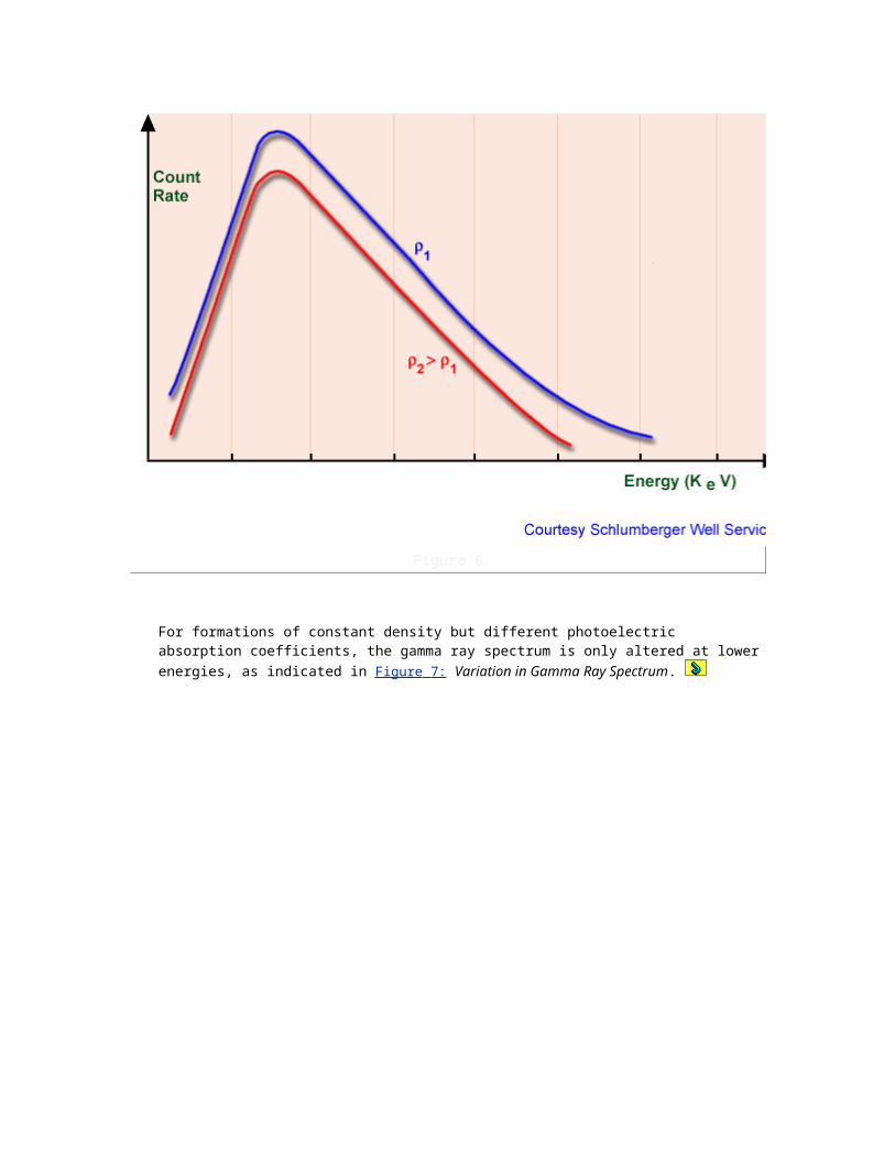
Figure 2

This graphic shows a schematic of a CNL tool eccentered in a borehole. The detectors are located at 15 and 25 inches from the source. The far detector has a larger volume than the near detector, to maintain adequate count rates. The tool measures the rate at which the thermal neutron population decreases from the near to the far detector. A very strong neutron source (16-Curie) reduces statistical variations and permits longer spacings. This in turn increases the zone of investigation. A large bow-spring ensures eccentering of the tool and optimum contact with the borehole wall. The CNL-G version has two epi-thermal detectors in addition to the thermal detectors at the other side and closer to the source. An illustration of the CNL may be seen in Figure   3 : CNL-G Dual Compensated Neutron Configuration.

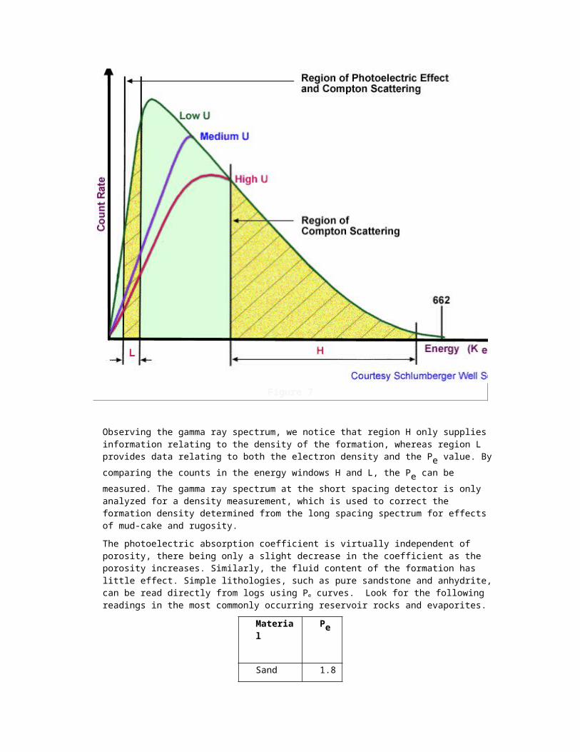
Figure 3

Conventional compensated neutron tools can be run equally well in open or cased, liquid-filled holes. In an empty hole (gas filled), the thermal neutron detectors do not work, and epithermal neutron tools are required. It is normal practice to run these tools in combination with the density and gamma ray tools. Conventional stacking arrangements are shown in Figure   4: Stacked Tool Arrangements for A) Running a Gamma Ray, Compensated Neutron and Compensated Density Log and B) Running a Casing Collar Locator, Gamma Ray and Compensated Neutron Log.

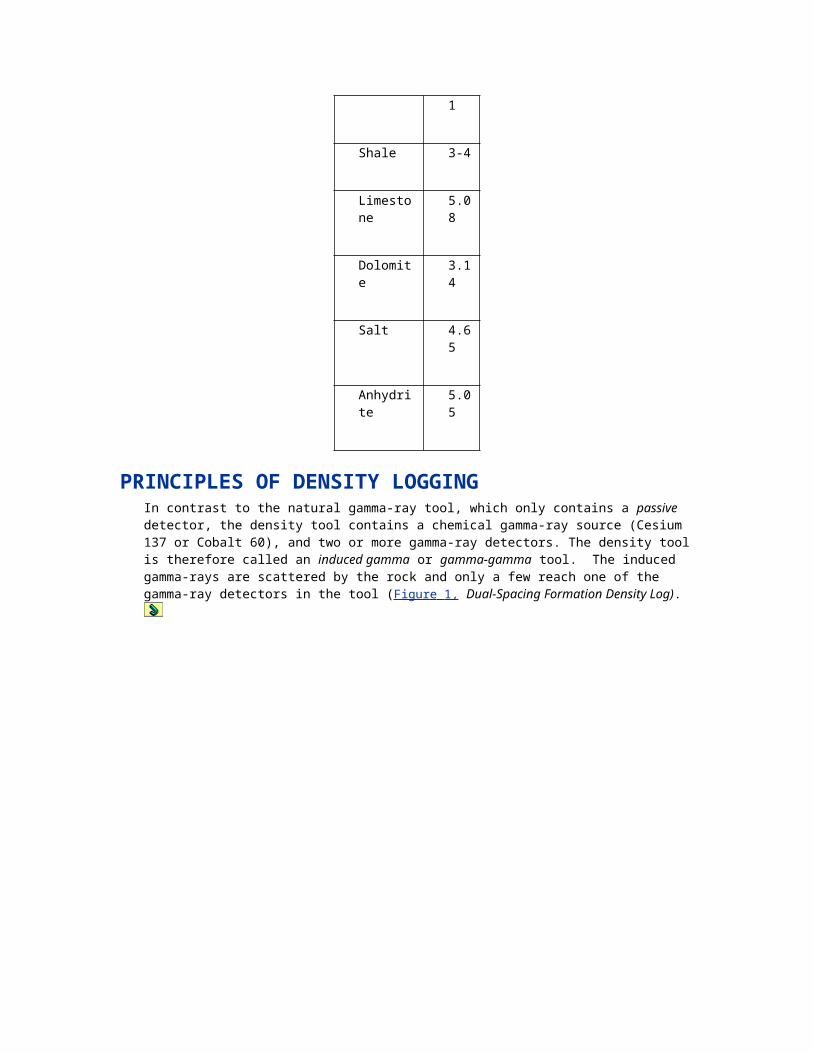
Figure 4

Of the two typical tool string arrangements, one (combined with density and gamma ray) is used for openhole jobs, and one (combined with a collar locator) for cased holes. Figure   5: Example of a Compensated Neutron Log (CNL) shows a combination compensated neutron/formation density log.

Figure 5

As in the case of density logs, compensated neutron logs may be used as direct indicators of porosity only in clean, liquid-filled, porous formations. The response in shaly or gas-bearing formations calls for special handling.

CNL OPERATING PRINCIPLETo properly understand the operation of the CNL logging tool, we must first understand the distribution of thermal neutrons as they move away from their source. The thermal neutron flux is defined as the number of thermal neutrons crossing unit area in unit time. This flux is controlled by the hydrogen content of the formation. Hydrogen is found in the water molecules filling the pore space (assuming that the formation is water-bearing). Thus the hydrogen content of the formation is a direct indication of its porosity.

Figure   6: Thermal Neutron Distribution as a Function of Distance from the Source shows a plot for three different values of porosity of the thermal neutron flux as a function of the distance from the source.

Figure 6

Note that the lines intersect at some distance from the source. At points closer to the source than the intersection, high thermal neutron flux means high porosity, but at points farther from the source, high thermal neutron flux indicates low porosity.

The absolute count rate is a poor indication of porosity; too many factors affect it. The actual count rate seen at any detector spacing from the source is a function not only of porosity, but also of such environmental factors as hole size, mud weight, and casing size and weight. Therefore, the CNL reading must be normalized to correct for unknown environmental effects. This is done by taking two readings of thermal neutron flux at different spacings and using them to define the slope of the response line. This slope is relatively unaltered by environmental effects, although the position of the response line on the graph may vary substantially in the "y" direction. Figure   7: CNL Borehole Compensation illustrates this concept.

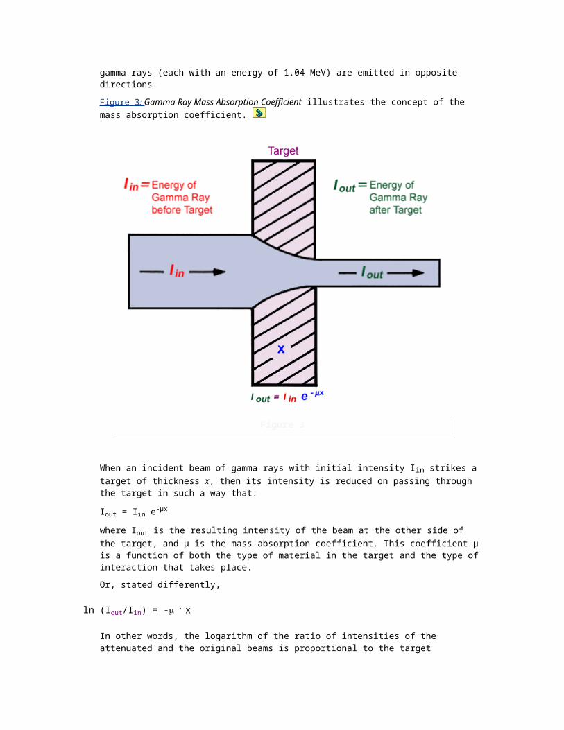
Figure 7

The primary measurement of the CNL tool is thus a ratio of two count rates. A high ratio indicates high porosity. The conversion of the ratio to a porosity value is based on laboratory experiments conducted with rock samples of known porosity. Figure   8: Tool Response for Sandstone, Limestone, and Dolomite Laboratory Formations shows the results of such experiments.

Figure 8

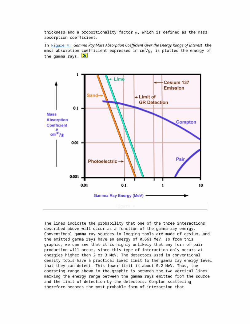
To record porosity directly, the ratio must be converted into porosity. For example, a ratio of 2.0 could mean less than 10% porosity in dolomite or more than 20% in sandstone. The surface controls for the CNL tool allow the operator to select the matrix for which a porosity is required. A convenient standard for the neutron tool is the limestone neutron porosity index. This index represents the same value that the tool would have read if it had been recorded on a limestone scale. Figure   9: Neutron Porosity Equivalence Curves plots the porosity measured by the neutron tool using a limestone, water-filled matrix against the true porosity for the indicated lines of constant lithology.

Figure 9

This chart shows that the relationship between apparent limestone porosity and the porosity values for dolomite and sandstone is fairly uniform, with the exception of the very high and the very low porosity values. In midrange apparent limestone porosity values, certain approximate rules of thumb can be used. Thus, if the CNL is run on a limestone setting, the conversion of ratio to porosity follows the middle of the three response lines.

Compensated neutron tools run on a matrix setting that is chosen by the logging engineer or the company witness. If the actual lithology coincides with the chosen matrix setting, then porosities may be read directly from the log. However, this is seldom the case and in many instances, the lithology is not known prior to logging the well. If the matrix is something other than that used in running the log, the porosity reading from the log will not be correct.

For instance, if tool was run on a limestone matrix, but the operator subsequently discovers that the actual matrix is not limestone, then it will be necessary to convert the apparent limestone porosity to some other matrix porosity. Correction charts such as the Neutron Porosity Equivalence Curves make this a relatively easy task. This chart can be used to determine the true porosity if the actual lithology is known. To obtain the true porosity, enter the measured porosity value on the x-axis, proceed vertically to the appropriate lithology line, then read the true porosity to the left, on the y-axis.

ACCELERATOR POROSITY SONDE (APS)The Accelerator Porosity Sonde (APS) makes thermal and epithermal neutron measurements to determine formation hydrogen content with minimal influence from formation atom density. In contrast with all foregoing neutron tools, this instrument has an accelerator (minitron) neutron source, instead of a chemical source. Along with a pulsed neutron accelerator, the tool features one thermal and four epithermal neutron detectors. The tool measures epithermal neutron ratio porosities (which are not affected by fluid salinity), as well as formation capture cross-section (sigma, S) and epithermal neutron slowing down time. The neutron porosity measurements can be corrected for tool standoff, and have a vertical resolution that is comparable to density and resistivity measurements.

The 14-million electron volt (MeV) accelerator emits eight times as many neutrons as the conventional logging source; furthermore, these neutrons have three times as much energy as those emitted by a conventional source. This increased neutron population makes epithermal neutron detection possible without compromising counting statistics. The APS neutron accelerator also improves wellsite safety by eliminating the radioactive source used by conventional neutron porosity tools. (In fact, the APS was seen as a way to obtain better porosity readings while complying with strict environmental and safety regulations.)

Neutron detector geometry has been improved to reduce lithology effects, increase sensitivity to gas in shaly reservoirs, and reduce borehole effects. Like previous epithermal neutron porosity tools, the APS sonde contains near and far detectors; however, it has two additional epithermal detectors (called the epithermal array), as well as a thermal detector (Figure   10: APS configuration). This construction produced a stable epithermal neutron tool, which can be run at logging speeds that are compatible with the density tool.

Figure 10

The tool combines the responses of the various detectors to compensate for lithology and matrix density effects.

The near-to-far measurement exhibits greater shale and gas effects, and provides a response that is similar to that of conventional compensated neutron tools.

The near-to-array measurement, which has a vertical resolution of 1 foot, is used to determine formation porosity.

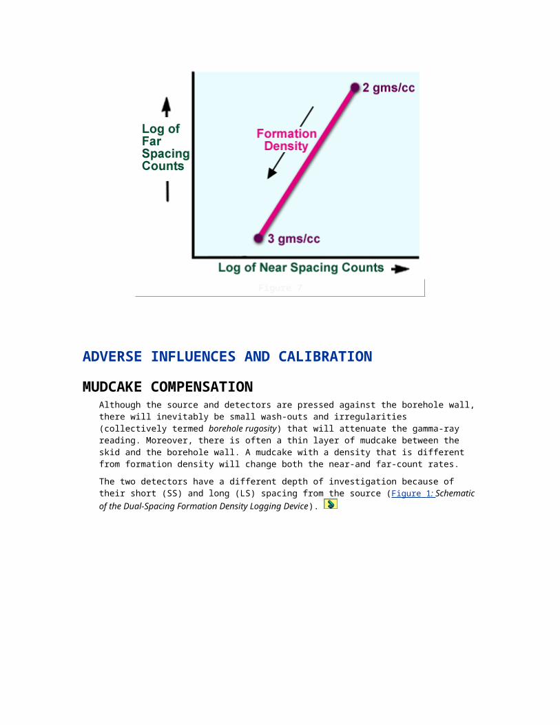
Epithermal array detectors monitor and correct the effects of tool standoff.

The thermal detector determines S by detecting neutrons rather than the gamma rays detected by conventional pulsed neutron tools. This neutron detection, along with detector shielding from the borehole, improves vertical resolution and provides a sigma value that is relatively free of borehole effects.

By comparing the readings of the near-to-array against the near-to-far detectors, it is possible to identify gas effects on the near-to-far reading. The gas effects can thus be used to call attention to gas zones in the well. In shaly formations, the APS tool uses the additional boost in apparent near-to-far porosity caused by increased atom density of clay minerals to improve the evaluation of clays.

Acoustic Logs

OVERVIEWAcoustic tools measure the speed of sound waves in subsurface formations. While the acoustic log can be used to determine porosity in consolidated formations, it is also valuable in other applications, such as:

Indicating lithology (using the ratio of compressional velocity over shear velocity),

Determining integrated travel time (an important tool for seismic/wellbore correlation),

Correlation with other wells

Detecting fractures and evaluating secondary porosity,

Evaluating cement bonds between casing, and formation,

Detecting over-pressure,

Determining mechanical properties (in combination with the density log), and

Determining acoustic impedance (in combination with the density log).

A typical acoustic log is illustrated in Figure   1: Sonic Log.

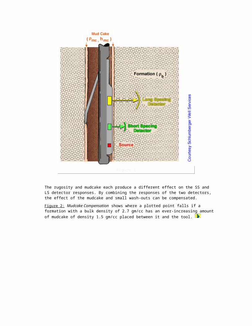
Figure 1

Curves recorded on acoustic logs may include the interval transit time, caliper, gamma ray and/or SP, and integrated travel time. The primary measurement of interest will be the interval transit time (t), measured in microseconds per foot (µsec/ft) which is the reciprocal of the velocity of a compressional sound wave in feet per second.

Integrated travel time is presented as a series of pips located immediately to the right of the depth track. Short pips represent 1 ms of travel time, with a large pip every 10 ms. Integrated travel time is used to help tie well depth to seismic sections. Travel time between two depths is obtained by counting the pips in the interval between the two points.

Tools used to acquire this measurement include the borehole-compensated tool, a slim tool version that can be run through tubing; and the long-spacing sonic tool. These tools include transmitter transducers that convert electrical energy into mechanical energy and receiver transducers that do the reverse. In its simplest form, the measurement is made in an uncompensated mode (Figure   2: Borehole Compensated Sonic Tool illustrates the principle of

this logging tool.

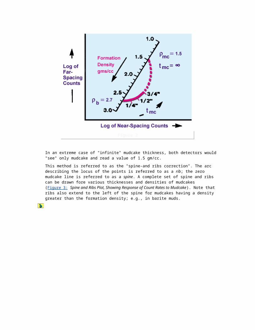
Figure 2

The BHC sonic tool used multiple transmitters and receivers to obtain two values of t, which were then averaged. The net result of this system was the elimination of errors in t due to sonde tilt and hole size variation. Even so, there were practical limits to the working range of the tool (e.g., in large holes).

The long-spacing sonic tool was next introduced in an attempt to overcome borehole environmental problems by reading acoustic travel time deeper within the formation and further from the borehole. Deeper investigation required a longer transmitter-receiver spacing, so long-spacing sonic tools typically have a transmitter-receiver spacing of 8, 10, or 12 ft.

POROSITY DETERMINATIONInterval transit time for a formation depends on lithology and porosity. Where lithology is known, it becomes a relatively easy task to determine porosity. We will discuss equations used to determine porosity in the next section.

Correlation

The sonic log makes a very good correlation tool with other sonic logs from offset wells, owing to the high vertical resolution of the tool and the fact that velocity variations in different types of rock produce a sonic log curve with a correlatable character.

PRINCIPLES OF ACOUSTIC LOGGINGThe sonic or acoustic log was developed in the 1950's to provide a detailed record of acoustic velocities along a well trajectory. If interval travel times and depth intervals corresponding to those travel times were recorded, then a velocity depth profile could be constructed. This profile could then be used to convert seismic events, recorded in two-way travel times, to images that were plotted as a function of depth.

It soon became apparent that the sonic travel times could also be used for other purposes, such as porosity estimation and gas detection -as well as lithology assessment when used together

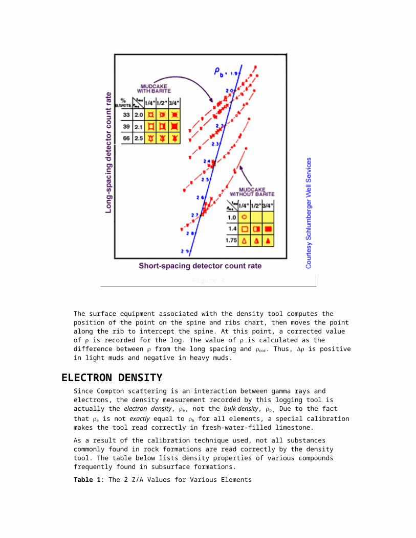
with density and neutron tools. Most important of all, the sonic tool can be used to evaluate mechanical properties of the rock when used in conjunction with the density tool.

As a porosity tool, the sonic wireline device was often run in combination with the SP-Gamma Ray-Resistivity tool string. Because this combination of tools was slick, and did not require pad contact, it was generally the first set of tools to be run in the hole during a log run. As such, the sonic log often provided the first indication of porosity during the log run. With advances in seismic prospecting and improvements in acoustic logging, the sonic tool is now enjoying a resurgence in seismic applications.

This discussion focuses primarily on how the sonic tool is used to evaluate porosity, and briefly touches upon mechanical properties and seismic applications. For information on other sonic applications, refer to the following IPIMS discussions on borehole velocity measurements and borehole visualization:

Discipline Series Topic Subtopic

Petroleum Geophysics 3-D Seismic and Other Geophysical Methods Other Geophysical Techniques Borehole Velocity Measurements

Formation Evaluation Wireline Well Logging Borehole Imaging Borehole Imaging Technology

PRINCIPLES

Two types of body waves travel within the formation:

Compressional waves, or P-waves, are waves of compression and expansion in which small particle vibrations occur in the same direction the wave is traveling. The compressional wave can propagate through both solids and fluids. P-wave data is acquired by conventional sonic tools for evaluating formation porosity.

Shear waves, or S-waves, are waves of shearing action in which rock particle motion is perpendicular to the direction of wave propagation. Only in a solid medium that has rigidity can the motion of the particles perpendicular to the wave propagation be accommodated. Hence the shear wave can only exist in solids and not in fluids. This is because solids have shear strength while liquids do not. Shear data is used in such applications as rock mechanics, formation anisotropy, permeability, and formation fluid evaluation.

The speed of P-and S-waves is controlled by rock mechanical properties, such as rock density and elastic dynamic constants. In fluid-saturated rock, these properties depend on the amount and type of fluid present, the composition of rock grains, and the degree of inter-grain cementation. Because soft, loosely consolidated rock exhibits smaller elastic stiffness, sound waves will travel slower in soft rock than in hard rock.

In acoustic logging, an acoustic pulse -produced by alternate expansions and contractions of a transducer -is emitted by a transmitter. A typical pulse of this sort is shown in Figure   1 (Typical transmitter pulse; courtesy of Schlumberger Well Services).

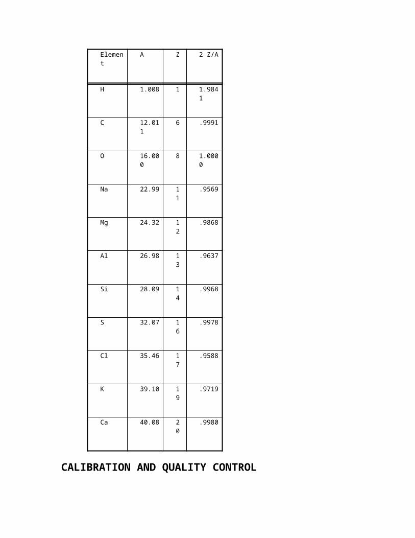
Figure 1

Part of the acoustic energy traverses the mud, impinges on the borehole wall at the critical angle of incidence, passes along the formation close to the borehole wall, reenters the mud, and arrives at a receiver, where it is converted into an electrical signal (Figure   2 Signal generated at the receiver by various wave arrivals; courtesy of Schlumberger Well Services).

Figure 2

The sonic tool has at least one pair of transmitters and receivers, as depicted in Figure   3: Acoustic Pulse Recording in a Borehole. A magnetostrictive alloy or piezoelectric crystal with a resonance frequency between 5 to 20 kHz is used as material for these transducers.

Figure 3

The transmitter sends out pulses with an oscillatory waveform that generates either compressional or shear waves.

The compressional (P) wave generated by the transmitter in the borehole fluid will travel in all directions until it hits the borehole wall. At the borehole wall the P-wave will continue in the rock as a fast P-wave, but some of the P-wave energy at the wall will be converted to a shear (S) wave in the rock. (Although both waves will expand in all directions from the point of impact, only the path along the wall is sketched in the above graphic of the Acoustic Pulse Recording. The wave traveling along the borehole wall will continuously produce compressional waves back into the borehole as indicated by the small arrows.

However, the velocity of the wave-front in the formation will out-run the P-waves created in the borehole because the P-wave velocity of the formation is higher than velocity of the borehole fluid. The P-wave that travels the shortest distance through the mud will be the first one to arrive at the receiver (known as the first arrival).

The shear (S) wave front travelling along the borehole wall will also create secondary P-waves in the fluid, since a fluid can only sustain compression waves and has no shear strength. As a result, there is a continuous conversion of S-waves back into P-waves along the borehole wall. The shortest P-and S-wave paths will not be identical, due to refraction of the waves on the borehole wall. According to Snell’s law, the slow S-wave will refract less to the normal than the fast P-wave.

As depicted the above graphic, the P-wave which represents the converted S-wave will arrive later than the leading P-wave ("first arrival" or "first break") which represents the P-wave velocity of the formation.

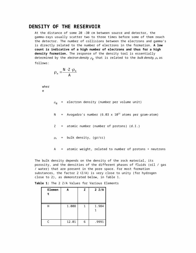
This first P-wave arrival is what triggers the sonic tool to record. The tool transmits about ten pulses per second, and the time is measured between the transmission and the first arrival. The actual parameter measured is the reciprocal velocity, called travel time (t), expressed for convenience in microseconds per foot.

With the velocity V, expressed in feet per second and t in sec, the following relation is valid:

 V

10=t

6

 The velocity of the compressional wave depends on the elastic properties of the rock matrix and the fluids in the pore space. The measured travel time is therefore a function of the rock matrix, the fluid type and the porosity.

ACOUSTIC TOOL DESCRIPTION

Early tools included only one transmitter and one receiver (Left hand side of Figure 4: Older Sonic Tools) embedded in a sonde body consisting of rubber (for low velocity and high sonic attenuation).

Figure 4

In this graphic, the sound pulse travels through the mud (A) at relatively low velocity. The compressional wave is refracted at the formation face and passes through the formation at formation velocity (B). The last leg (C) is again through the mud. The measured travel time is therefore too long due to the passage through the mud. Additionally, the physical length of B is not constant, since changes in velocity alter the refraction angle.

Later versions (Right hand side of the Older Sonic Tools graphic) incorporated one transmitter and two receivers, a few feet apart, to cancel the above problems. This system measures, in effect, only the time required to travel interval D, assuming intervals C and E take the same travel times. In that case, distance D, which is the distance that the P-waves traveled in the formation, is equal to the spacing R1 -R2. The only serious shortcoming of this system is that distance C is not equal to E when the tool is tilted in the hole (Left hand side of Figure   5: Tilted Sonic Tool and the Borehole Compensated Sonic Tool) or when the hole size changes over short intervals.

Figure 5

BOREHOLE COMPENSATED SONIC

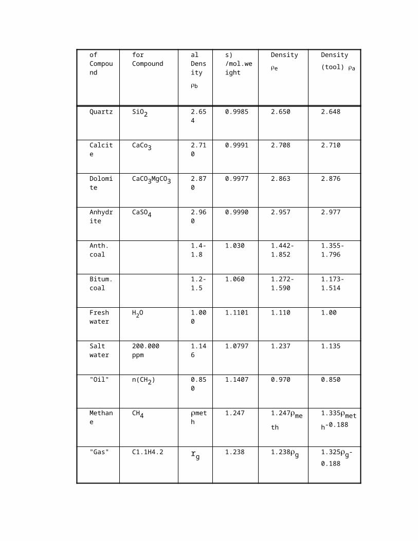
Still later versions of the sonic tool, like the Borehole Compensated tool (BHC), incorporated two transmitters and four receivers (Right hand side of the Tilted Sonic Tool and the Borehole Compensated Sonic Tool graphic). The transmitters are pulsed alternately, and t values are obtained from alternate pairs of receivers. The two t values are averaged to cancel differences in the C and E distances caused by tool tilt. The tool consists of a slotted metal body housing, which causes the sonic wave traveling through the tool to follow a tortuous path, thereby arriving later than the wave that travels through the formation or the wave that travels directly through the mud.

Overall, the net result of this system is the reduction of errors in t that are caused by sonde tilt and hole size variation.

Even so, there are practical limits to the working range of the tool (e.g., hole size). In large boreholes, the time taken for a compressional wave to travel from the transmitter to the formation, through the formation, and back through the mud to a receiver may exceed the time taken for a direct transmission from the transmitter to the receiver through the mud. The critical factors affecting this condition are transmitter-receiver spacing, hole size, and travel time within the formation. With conventional borehole-compensated acoustic tools that have a 3-ft spacing, the highest t formation that can be measured is 175 µs/ft in a 12-1/4 inch bore hole, and 165 µs/ft in a 14-inch hole. This limitation is not serious if the formation is a reservoir rock with a t in the normal range of 40 to 140 µs/ft. It does become a serious defect if the rock is a shale of long transit time, and the purpose of the log is to compute integrated travel time for geophysical purposes.

LONG-SPACING ACOUSTIC TOOL

The long-spacing acoustic tool was introduced in an attempt to overcome environmental problems. When a shale formation is drilled, the shales exposed to the mud frequently change their properties by absorbing water from the drilling mud. This results in a change in travel time for elastic waves. In order to read the travel time in the undisturbed formation away from the borehole, a longer transmitter-receiver spacing is required. Typically, a long-spacing acoustic tool will have transmitter-receiver spacings of 8, 10, or 12 ft. Figure   6: Comparison of BHC and LSS Sonic Logs shows a comparison of a conventional borehole-compensated acoustic log with a long-spacing acoustic log.

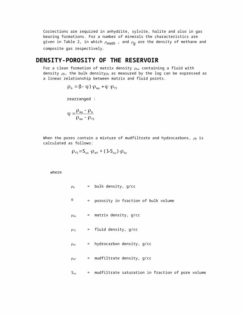
Figure 6

Lengthening the spacing on an acoustic device achieves two ends:

A valid acoustic log may be recorded in a bigger hole with a long-spacing device than with a conventionally spaced tool.

The zone investigated by the tool is deeper into the formation with a long-spacing device than with a conventionally spaced tool.

Deeper investigation into the formation is needed when logging through shale intervals that have been altered by the drilling process. Provided that t of the formation in the undisturbed state is less than t of the formation in the altered state, the quickest route for a compressional wave is via the undisturbed formation, or deep within the formation. Figure   7 : Depth of Investigation of Long- and Short-Spacing Sonic Tools illustrates this effect.

Figure 7

The long-spacing tools make their measurements in a "depth-derived" mode. That is, the borehole compensation is actually achieved by memorizing travel times that are measured when the tool is at one depth, and combining those with travel times recorded at a shallower depth when an alternate combination of transmitters and receivers is activated. (The long-spaced sonde would be too long if used in the same configuration as the BHC tool.) Two transmitters spaced 2 feet apart are located 8 feet below a pair of receivers that are also 2 feet apart Figure   8 : Long-Spaced Sonic "Depth Derived" Principle).

Figure 8

Memorizing the first t reading and combining it with a second t reading (measured after the sonde has been pulled the appropriate distance farther along the borehole) compensates for the hole size changes.

MONOPOLE SONIC TOOLS

The pressure source in monopole sonic tools creates an omni-directional compressional wave pulse in the borehole fluid. This compressional wave pulse subsequently propagates out into the formation. The compressional pulse causes a slight uniform bulge around the borehole wall, and excites compressional and shear waves in the formation. These compressional and shear waves, in turn, produce head waves in the borehole fluid. Receivers in the monopole tool work by detecting head waves in the borehole fluid, rather than detecting formation compressional and shear waves.

Head waves exist only when formation waves propagating up the borehole travel faster than the waves created in the borehole fluid. Compressional waves always move faster through the formation than through fluids, so the receiver on the monopole sonic tool has no problem recording the compressional head wave.

However, shear waves can present problems for the monopole tool. In slow, poorly consolidated formations, the shear wave velocity in the formation is usually less than fluid wave velocity, which prevents the formation of head waves in the borehole fluid. Without shear head waves in the borehole fluid, the monopole tool is unable to detect shear waves in slow formations.

DIPOLE SONIC TOOLS

Dipole tools measure wave components that propagate deep into the formation. Unlike monopole tools, the dipole tool is capable of recording borehole shear/flexural measurements in soft or hard (slow or fast) formations. As opposed to the omni-directional source used by monopole tools, the dipole tool uses a directional source to create a pressure increase on one side of the hole and a decrease on the other. This causes a small flexing of the borehole wall, which directly excites compressional and shear waves in the formation. Propagation of this flexural wave is coaxial with the borehole, whereas displacement is at right angles to the borehole axis and in line with the transducer.

The compressional waves and shear waves radiate straight out into the formation. However, an additional shear/flexural wave, initiated by the flexing action of the borehole, propagates up the borehole. The shear/flexural wave, is dispersive -its velocity varies with frequency. At low frequencies, it travels at the same speed as the shear wave; but at higher frequencies it travels at slower speeds. The shear/flexural wave creates a dipole-type pressure disturbance in the borehole fluid, which is detected by the tool’s directional receivers.

FULL WAVEFORM TOOLS

Full waveform sonic tools are used to record the entire acoustic wavetrain. This waveform data can then be processed to obtain compressional, shear, and Stoneley slowness, shear wave and compressional wave amplitudes, and Stonely wave attenuation. Using this information, it is possible to evaluate rock types, gas zones, porosity, fractures, formation elastic properties, permeability and acoustic impedance.

The log in Figure   9 (Full waveform sonic log; courtesy of Halliburton Energy Services) presents the raw waveform in the right-hand track; with shear and compressional slowness in the middle track; and gamma ray, caliber and receiver gain in the left-hand track.

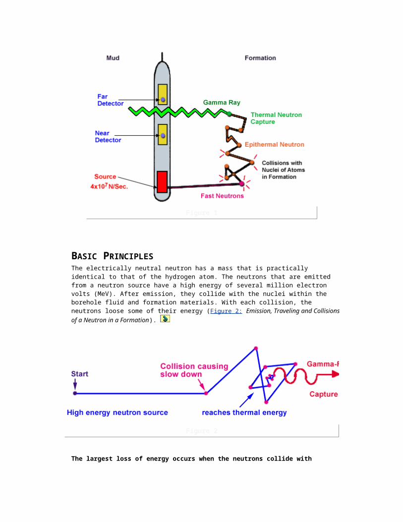
Figure 9

(This logging tool automatically adjusts receiver gain after each transmitter pulse to prevent signal clipping. This preserves all phases of signal amplitude by increasing the gain in soft formations and reducing gain in less-attenuating, hard-rock formations.)

Because receiver gain is inverse to the attenuation of the highest amplitude measured in the waveform (usually the Stoneley wave), the gain curve (which indicates the gain applied by the tool) can be used to detect natural fractures, borehole washouts, and lithologic changes. Of particular interest are fractures, which are characterized in waveform plots by:

a marked decrease in the amplitude of Stonely waves,

moderate attenuation of the shear waveform, and

little or no change in the compressional and shear slowness.

In Figure   10 (Full waveform log of a fractured carbonate; courtesy of Halliburton Energy Services), we see how waveform data are used to evaluate changes in the acoustic signal.

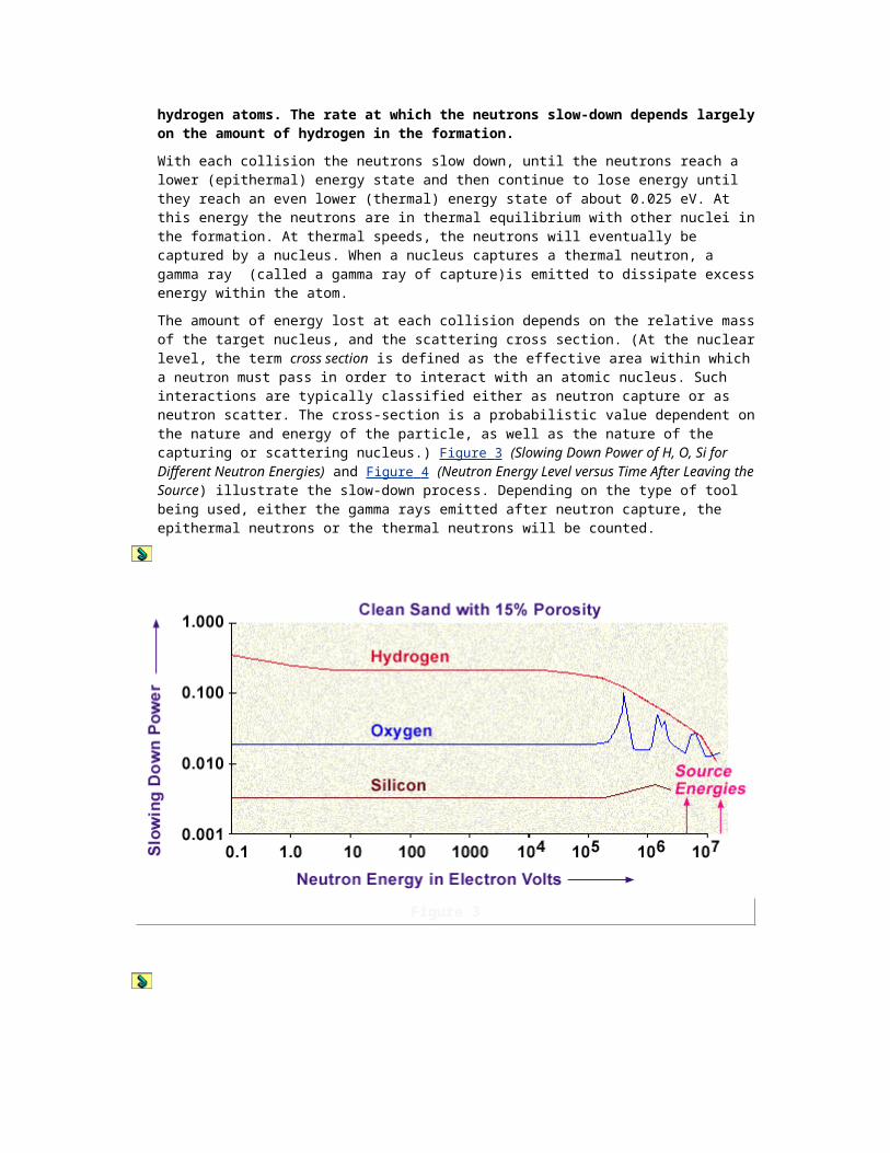
Figure 10

These changes are caused by acoustic absorption or dispersion effects and point to geological discontinuities such as fractures, faults, or thin beds. Such indicators are found by measuring the amplitude, phase, and frequency of the waveform energy. Next, a special color-coding technique is applied to these characteristics in order to identify and enhance formation response to the acoustic signal.

The right-hand track of the log presents acoustic transmissivity, measured in decibels. Transmissivity is a direct measurement of the attenuation of acoustic energy within the formation. Any formation changes which cause absorption or dispersion of acoustic energy will affect transmissivity. Shear and Stoneley transmissivity, in particular, will decrease in the presence of fractures. On this log, the blue shading indicates highly attenuated waves, while red shading is applied to the lesser attenuated portions of the acoustic wave. On this log, we see strong attenuation of the shear and Stoneley regions across the intervals from XY215 feet to XY240 feet, and from XY295 to XY310 feet, thus indicating highly fractured zones.

SONIC LWD TOOLS

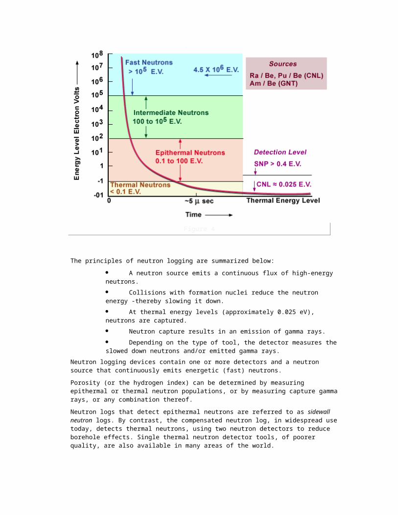
Of the impressive assemblage of Logging While Drilling tools, the sonic device was one of the later tools to be developed. With today’s LWD sonic tools, it is possible to obtain wireline-quality measurements, often before the onset of borehole washouts and invasion. These tools record full waveforms, and are capable of generating compressional and shear slowness logs in both fast and slow formations. Figure   11 (Bi-modal Acoustic LWD Sonic Tool, courtesy of Halliburton Energy Services) shows an example of one such tool, offered by Sperry-Sun Drilling Services.

Figure 11

The LWD sonic tool contributes a new dimension to real-time evaluation of the formation and its effect on drilling parameters. When combined with other logs from a conventional LWD logging suite, the sonic tool can be used in many cases to help the geologist evaluate pay zones prior to invasion, and can help the driller to recognize pressure trends and optimize mud weights for increased drilling efficiency. With transit times provided by the LWD sonic tool, it is possible to generate current synthetic seismograms to help the geophysicist to correlate present well trajectory with surface seismic data.

Applications of the LWD sonic tool are similar to those of traditional openhole sonic tools, and include:

Petrophysics -Porosity determination, Gas detection, Complex lithology evaluation.

Drilling -Real-time pore pressure determination, Rock strength calculations, Bit wear predictions, Borehole stability analysis.

Geophysics -Near real time synthetic seismograms, Time-to-depth seismic correlation while drilling, AVO analysis.

ADVERSE INFLUENCESAcoustic logs are subject to errors which are often very easy to detect. Factors that influence sonic log readings are:

Noise spikes; causing decreased travel times

Stretch; causing excessive travel times.

Cycle skipping causing excessive travel times.

Hydrocarbon effect -causing increased interval transit times.

Shale effect -causing increased travel times

Unconsolidated sands -causing excessive travel times

Boreholes without liquid -will not support propagation of compressional waves, and thereby preclude use of the sonic tool.

Conventional acoustic tools that measure travel times contain a threshold circuit which triggers when the received signal passes beyond a pre-set limit. The limitations of the conventional tools are all associated with either this trigger mechanism, the shape of the waveform that is detected, or the tool calibration. In some cases, however, the problems are readily apparent, and can be cleared up by simply logging at a slower speed.

NOISENoise can be generated mechanically or by stray electric signals that are picked up by the receiver electronics (Figure   1: Noise Spikes). If this noise exceeds the trigger level A before the arrival of the P-wave that traveled through the formation, the receiver circuit will be triggered prematurely and the time measurement will be erroneously small.

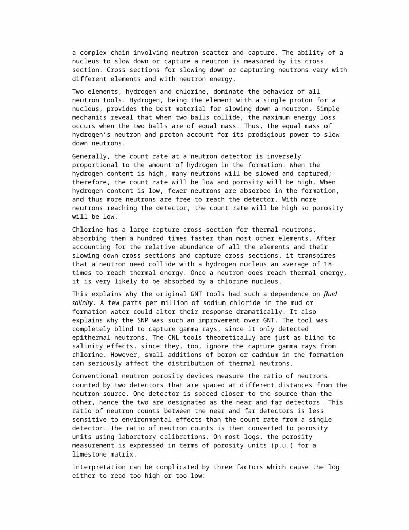
Figure 1

To limit this possibility all receiver circuits are switched off for 120 microseconds after transmitter firing. The far receiver is the most sensitive due too longer "open" periods and the larger attenuation of the acoustic wave for longer spacings. Noise spikes are usually intermittent and lead to much smaller travel times over very short intervals. The log readings around these noise induced short travel times can usually be trusted. Editing out noise peaks is very important for seismic applications where a cumulative travel time that is too short will lead too horizons that are located too deep in the seismic section after two way travel times are converted to depth.

DT STRETCHThe second and third cycle of the wave-form are usually of progressively larger amplitude. As depicted in the Noise Spikes graphic, the signal arriving at the far receiver is usually weaker. As the trigger level is constant for both receivers, triggering at the far receiver can occur too late, causing t to be slightly too large. This phenomenon sketched in Figure 2:

Figure 2

Sonic Stretch is called t (DT) stretch.

CYCLE SKIPPINGWorse than DT stretch is the occurrence of triggering at the second or even third cycle (Figure   3:

Cycle Skipping).

Figure 3

Cycle skipping leads to a marked sudden shift to a higher t value and later to a similar abrupt shift back to the correct value. This problem is often caused by the presence of gas, or fractures, or borehole rugosity. In this regard, cycle skipping should be regarded more as a diagnostic tool than as a nuisance.

The actual travel time measurement is determined at the first arrival peak. However, the tool’s internal trigger mechanism for detecting this peak is subject to errors. Figure   4 illustrates two

common problems.

Figure 4

In the first, the bias level is set too high and the travel time is triggered by a later peak, causing an erroneously long time to be measured (this is known as cycle skipping). In the second, the bias is set too low and the travel time is triggered by noise, causing an erroneously short travel time.

In the BHC mode, it is not always possible to distinguish between cycle skipping and noise, since two measurements are effectively averaged by the tool.

Cycle skipping is not a subtle problem; during logging it will be readily apparent on the logging screen when the curve starts jumping back and forth. In many cases, this problem can be rectified while logging by simply dropping back down, and then re-logging the interval at a slower speed. This approach will provide a valid and useable sonic curve from which to calculate porosity, etc; however, by removing the cycle skipping from a gas zone, the "flag" which called attention to the gas zone will also be removed.

HYDROCARBON EFFECTIn the presence of hydrocarbons, the interval transit time of a formation will increase, causing the sonic porosity to read too high. According to Hilchie (1978), the following empirical corrections should be applied to counteract the hydrocarbon effect:

 )(9.0

)(7.0

oil

gas

sonic

sonic

 

SHALE EFFECT

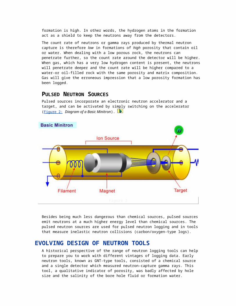
When logging through a sandstone, the presence of shale laminae will affect sonic porosity values. The t values usually increase in proportion to the bulk volume fraction of the laminae,

because tsh values of the shale are usually greater than tma values of the matrix.

EFFECT OF UNCONSOLIDATED SANDUnconsolidated formations exhibit longer travel times than can be accounted for by the Wyllie time average equation. This discrepancy can be handled in two ways: conventionally, and by the Hunt transform. The conventional method merely adapts the Wyllie time average equation by introducing the factor Bcp, such that

 

 where Bcp is some number greater than 1. This can be done by estimating Bcp from the transit time in shales adjacent to the formation of interest. Then

 Bcp= tshale / l00

 Thus, if, in a shallow sand-shale sequence, log shale is 130 µsec/ft, then a Bcp of 130/100, or 1.3,

should be used. The Hunt transform is based on empirical observations from sonic logs and porosity determinations from other means. Figure   5: Sonic Porosity Determination shows the

generalized form of the Hunt-Raymer transform compared to the Wyllie formula,

cpmaf

mas B

1

tt

tt

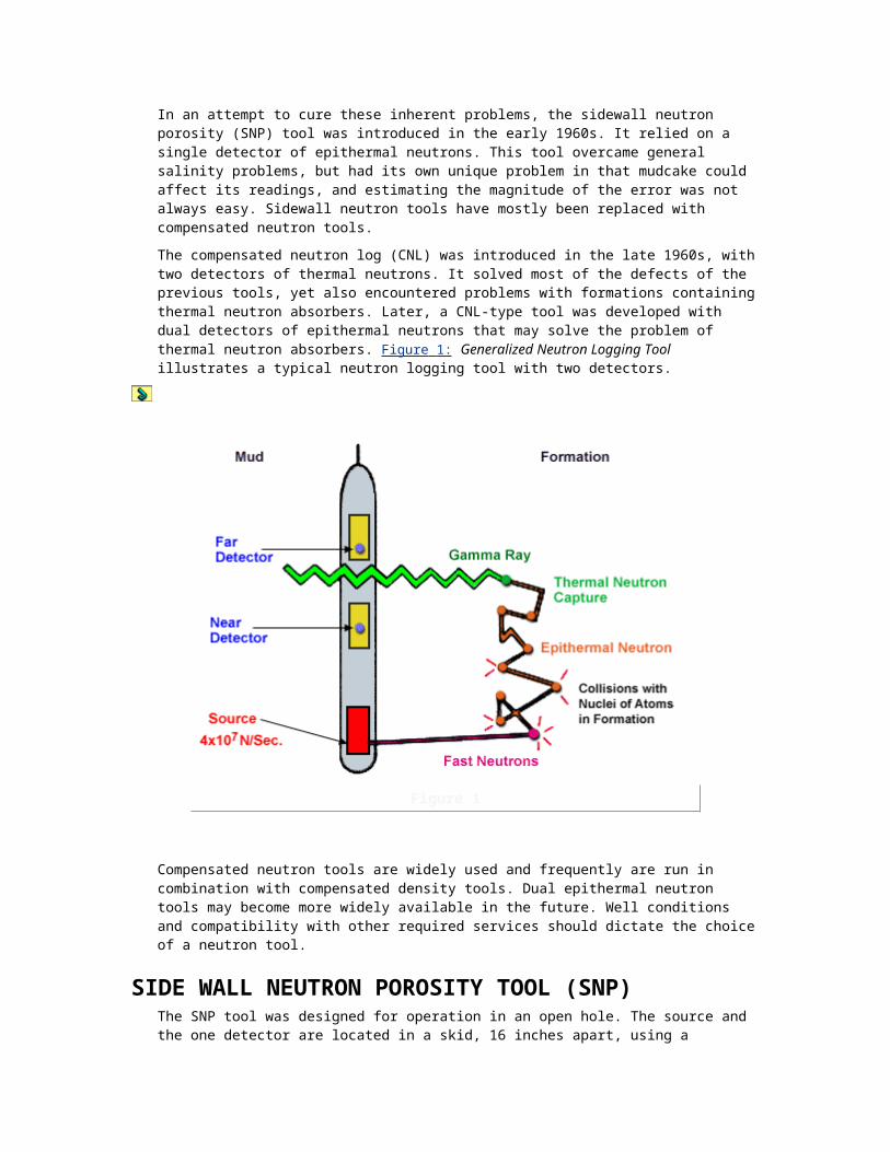
Figure 5

and plots t against porosity for sandstone, limestone, and dolomite. An acceptable equation relating porosity to t for this transform is given by:

  ma-1

)fma(

1S rr

 Note that t fluid does not appear as a term in this equation. The assumption is that the fluid is liquid (not gas) and is built into the coefficient 1/(rma -rf). In sandstones this coefficient is very close to 5/8.

PHYSICAL LIMITATIONSA graph of transmitter-receiver (TR) distance against the time to travel from T to R (Figure 6: Effect of TR Spacing, No Altered Zone) shows that the fastest sound path is through the mud at spacings less than critical spacing Xc.

Figure 6

For larger spacings, the wave path that takes the shortest time to travel, is the one that passes through the formation.

The formation velocity v1 is measured only when the spacing X1 is larger than Xc. However

assuming that the tool is centered in the hole Xc increases with increasing hole diameter D (larger mud-path Xm), or decreasing formation velocity v1 (slope 1/v1 becomes steeper, and Xc will be larger). A spacing, TR1, of 3 feet is usually sufficient to avoid these problems

An "altered" zone around the borehole can exist where the formation has sucked up mud-filtrate and as a result has a lower sonic velocity. Examples are soft hydroscopic clays. This low velocity zone can be circumvented in the same way as the low velocity mud layer by increasing the spacing between transmitter and receiver. However due to the smaller difference between the

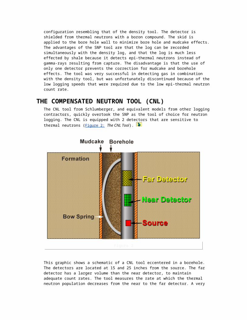
altered zone velocity and the undisturbed zone velocity the spacing has to increase substantially before the wave that travels through the high velocity undisturbed zone out-runs the wave through the low velocity altered zone.

The distance Xc even under these adverse conditions is seldom more than 10 feet, hence sonde spacings with this length usually produces accurate readings, whereas the BHC would give too high t readings. When the velocity of the shear wave is lower than the compressional velocity of the mud it is physically impossible for the shear wave to leave the formation. The shear wave should, according to Snell’s law for Vmud > Vforrmation , be refracted away from the normal but the wave that travels along the borehole has already an angle of 90° with the normal. Hence, for this case, the shear wave will not produce a secondary compressional wave in the borehole, and detection of the shear wave velocity with a conventional sonic tool is not possible. The critical shear velocity can be calculated with:

 formation

mud

mud

formation

V

V

)sin(

)sin(

in which the sin (formation) = 1 

CALIBRATION AND QUALITY CONTROLIt bears repeating that acoustic logs are subject to very easily detectable errors, such as cycle skips and noise. And many such problems can often be cured by simply decreasing the logging speed. However, even when the tool is triggering properly, we require proof that the recorded t is correct.

A true calibration test shows the response of the tool to a standard environment. An excellent check is to record the transit time in steel casing; where it should read approximately 57 s/ft (provided that the casing is not bonded to a formation of high interval velocity, such as a tight limestone). The tool can be checked in open hole below casing if the log is run through such marker beds as

salt (t = 67 µsec/ft)

anhydrite (t = 50 µsec/ft)

limestone (t = 47.6 µsec/ft).

As with all logs, a repeat section of at least 200 feet should be recorded, and this repeat section should overlay within a few sec of the main log over the same interval.

POROSITY AND OTHER APPLICATIONSGiven the wide range of signals obtained by modern wireline sonic logging tools (compression, shear, Stoneley, etc.), it is possible to apply sonic data to a variety of pursuits. Most of applications fall into 3 broad categories.

Mechanical Property Analysis: wellbore stability, perforation stability or sanding analysis, and hydraulic fracture height prediction, anisotropy evaluation

Formation Evaluation: gas detection, fracture detection, qualitative evaluation of permeability, and borehole visualization (for more information, see the Formation Evaluation Topic on Borehole Visualization).

Geophysical Interpretation: synthetic seismograms, vertical seismic profiling, calibrating AVO

In this section we will explain sonic porosity measurements, and review some of the other applications which depend on various sonic tools for their data.

The fact that compressional waves travel faster through solid matrix material than through fluid is the basis for the method used to determine formation porosity from sonic logs. Figure   1 : Sonic

Porosity Measurement gives a schematic in which the pore space and the solid matrix have been separated for the purposes of illustration.

Figure 1

If tf is the time taken to travel through the pore space and tma is the time taken to travel through the matrix, the total travel time measured will be t, and the porosity will be given by:

 t = tf + (1-) tma

 or 

 This is known as the Wyllie time average equation. Note that it is not an exact solution for porosity, but an approximation.

Matrix travel time depends on the matrix itself. The table below provides partial listing of interval travel times for matrix materials and fluids commonly seen in the borehole.

Table 1: tma for Common Matrix Materials and Fluid

Material orMedium

 

Travel Timet (μs/ft)

 

Velocity(ft/s)

 

Density (g/cc)

 

Dolomite

 

43.5

 

23000

 

2.87

 Limestone

 

47.5

 

21000

 

2.71

 

maf

masonic tt

tt

Sandstone

 

55.6

 

18000

 

2.65

 Anhydrite

 

50.0

 

20000

 

2.97

 Gypsum

 

52.5

 

19000

 

2.35

 Salt

 

67.0

 

15000

 

2.03

 Water (fresh)

 

200

 

5000

 

1.00

 Water (100,000 ppm NaCl)

 

189

 

5300

 

1.06

 Water (200,000 ppm NaCl)

 

176

 

5700

 

1.14

 Oil

 

232

 

4300

 

--

 Air

 

919

 

1088

 

--

 Casing

 

57

 

17000

 

--

 

Fluid travel time is a function of the temperature, pressure, and salinity of a solution. A commonly used default value for

tf is 189 µsec/ft.

Unconsolidated formations exhibit longer travel times than can be accounted for by the Wyllie time average equation. This discrepancy can be handled in two ways: conventionally, and by the Hunt transform. The conventional method merely adapts the Wyllie time average equation by introducing the factor Bcp, such that

 

 

where Bcp is some number greater than 1. This can be done by estimating Bcp from the transit time in shales adjacent to the formation of interest. Then

 Bcp=tshale / l00 

Thus, if, in a shallow sand-shale sequence, log shale is 130 µsec/ft, then a Bcp of 130/100, or 1.3,

should be used. The Hunt transform is based on empirical observations from sonic logs and porosity determinations from other means. Figure   2: Sonic Porosity Determination shows the

generalized form of the Hunt-Raymer transform compared to the Wyllie formula,

cpmaf

mas B

1

tt

tt

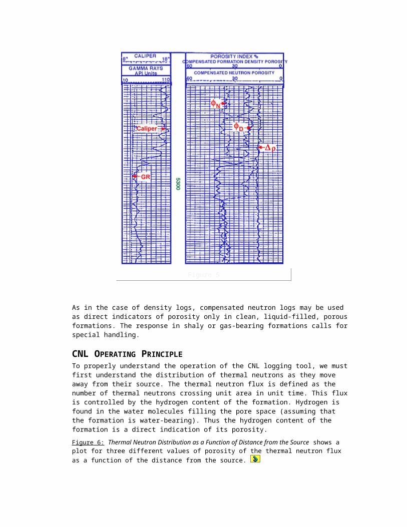
Figure 2

and plots t against porosity for sandstone, limestone, and dolomite. An acceptable equation relating porosity to t for this transform is given by:

  )t

t-1 (

)(

1 ma

fma

S

rr

 Note that t fluid does not appear as a term in this equation. The assumption is that the fluid is liquid (not gas) and is built into the coefficient 1/(rma -rf). In sandstones this coefficient is very close to 5/8.

SECONDARY POROSITYCarbonates often contain vugs or fractures that are much larger than the pore space which constitutes the primary porosity of the formation. In vuggy formations, the sonic tool predominantly logs the primary intergranular porosity. If total porosity (taken from neutron/density tools) is known, then the secondary porosity can be calculated by subtracting the value of sonic porosity from total porosity, thus leaving secondary porosity.

  sonictotalndry 2

 

DETECTION OF OVERPRESSURED ZONES

Compaction effects manifest themselves on sonic logs as a decrease of t with depth. This is particularly evident in shales. The deeper a shale is buried, the more compact it becomes and the shorter the t. In cases where there is no escape for the water contained within the shale, compaction ceases and over-pressure results. For this reason, an anomalously high t in a shale at that depth is generally an indicator of formation over pressure. Obtaining readings on a sonic log in shales only and plotting thesetsh values against depth yields a "normal" gradient. Departures from this gradient indicate overpressure.

FULL WAVEFORM RECORDINGThe long-spaced acoustic tool is capable of recording waveforms for later processing. The longer spacing allows a larger time separation for the compressional and shear wave arrivals.

The various transmitter-receiver combinations permit four waveforms to be recorded at 6-in. intervals. Figure   3: Long Spaced Sonic Waveform illustrates composite waveforms received at the near and far receivers when the upper transmitter is fired.

Figure 3

Digitization of the waveforms is normally made at a 5 sec sample interval for 512 samples, i.e., 2560 microseconds. A delay of 200 to 500 microseconds is selected by the logging engineer as an input parameter.

Waveform recording considerably extends the range of applications of acoustic logging both in open holes and cased holes. The principal benefit is determination of the shear wave velocity of the formation.

The objective of waveform processing is to distinguish between the compressional and shear wave arrivals and to measure their interval transit times. Furthermore, in cased holes, formation arrivals are usually distinct from casing arrivals, thereby permitting a viable acoustic measurement where previous acoustic devices would have been ineffective.

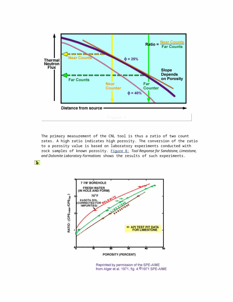
Data-processing methods used to extract shear wave arrival times are somewhat complex, and mirror seismic-processing methods; i.e., multiple waveforms are "stacked." Yet it is quite common to "see" shear arrivals on variable density displays of the sort shown in Figure   4: Variable Density Display with Compressional and Shear Wave First Arrivals Indicated.

Figure 4

VERTICAL SEISMIC PROFILE (VSP)Another seismic application related to the acoustic log is the vertical seismic profile (VSP). By suspending a geophone in the wellbore and actuating an energy source at surface, reflections of compressional waves may be recorded. Some of these arrive at the geophone after being reflected from beds below the bottom of the well. Thus the VSP affords a method of looking ahead of the drill bit. A schematic of the setup to make a VSP survey is shown in Figure   5: Setup for a VSP Survey,

Figure 5

and an example of the results in Figure   6: Results of a VSP Survey.

Figure 6

Special Open Hole Tools

Caliper Logs

The caliper log measures the diameter of the borehole. The first caliper logs were developed to determine borehole size in holes shot with nitroglycerin. These early logs showed large variations in hole size, even in the portions of the hole that had not been shot. This illustrated the need for the caliper log over the entire hole.

Methods of Recording Several types of caliper are currently in use. One type consists of three or four spring-driven arms that contact the wall of the borehole. The instrument is lowered to the total depth, and the arms are released either mechanically or electrically. The spring tension against the arms centers the tool in the well. The arms move in and out with the change in wellbore diameter. The arm motion is transmitted to a rheostat so that change in the resistance of an electric circuit is proportional to the hole diameter. The borehole diameter is recorded at the surface by measuring the potential across this resistance.

Another instrument uses three flexible springs that contact the wall of the borehole. These springs are connected to a plunger that moves up or down as the springs expand or contract with changes in borehole diameter. The plunger passes through two coils. When an alternating current is passed through one coil, an electromotive force (emf) is induced in the other coil. The amount of this induced emf is a function of the plunger position and is proportional to borehole diameter.

Both of these instruments may be adjusted to record borehole area rather than hole diameter. If the caliper log is used to determine hole volume, it is desirable to record area on a linear scale. If the caliper log is used to determine hole configuration, the hole diameter is recorded on a linear scale.

A third type of caliper log, the microcaliper, is discussed in connection with the electrical-log microdevices. This instrument uses two pads rather than arms or flexible springs. Hole diameter is determined by the movement of these pads, which are held against the borehole wall by springs.

Typical Configuration on the Borehole A schematic drawing of a typical borehole ( Figure   1 ) shows that some formations cave considerably, causing enlarged holes.

Figure 1

Other formations do not cave, and because of the presence of mudcake, the hole size may actually be reduced to less than bit size. Some formations (not shown here) may swell, causing reduction in hole size.

The primary cause of formation caving is the action of the drilling fluid, bit, and drillpipe. Most drilling muds, composed primarily of water, exert chemical action on shales (hydration of the shales), often causing them to disintegrate and slough into the hole. The amount and rate of this sloughing depend on the nature of the mud and shale. "Heaving" shales swell rather than disintegrate.

If a fresh-water mud is used to drill a salt section, it dissolves salt until the mud becomes salt-saturated. The drilling fluid does not "react" with rock such as limestone, dolomite, and sandstone. If those formations are permeable, however, a mudcake will rapidly form ( Figure   1 ). Mudcake character (density and thickness) varies with the mud used to drill the well, and its thickness is limited by erosion of the circulating drilling fluid.

If/when shallow portions of the hole are drilled with water, loosely cemented sands encountered may cave.

The action of the bit is not very important, but if a thin sand is surrounded by shales that have caved, the bit probably knocks off part of the sand ledge with each round trip.

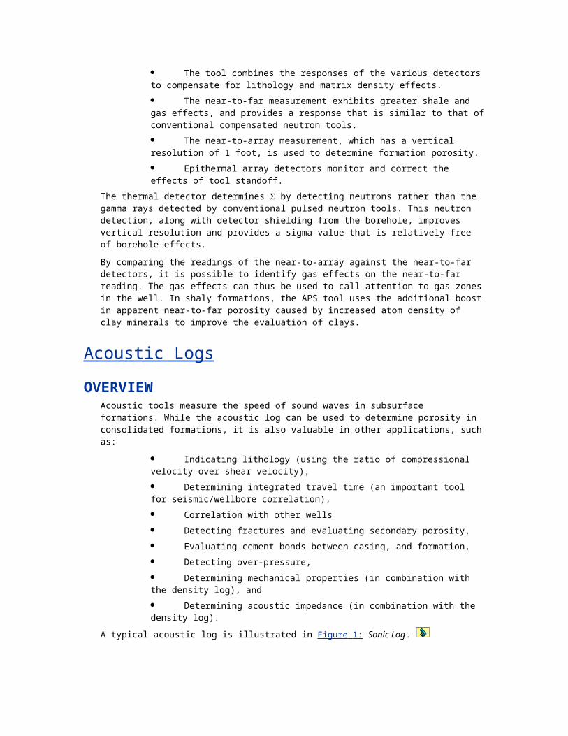
Action of the drillpipe against the side of the hole causes some enlargement even in sandstones and limestone. Though this enlargement may not be great enough to affect hole volume appreciably, it may cause keyseating and necessitate a fishing job. Formation "wear" by the drillpipe causes the hole to be noncylindrical, in which case a four-arm caliper will display the long and short axes of the hole.

Interpretation and Application of Caliper Logs

Caliper logs are usually recorded on vertical scales from 1 in. = 100 ft to 5 in. - 100 ft. The horizontal scale is selected to show a detailed picture of hole diameter and is usually in the order of 1 in. = 4 in. Because of the difference in scales, it is easy to get the impression from caliper logs that tremendous cavities are created. Keep in mind that when a normal borehole is plotted on the same horizontal and vertical scales, it is evident that it is quite "regular."

The primary uses of the caliper log are:

to compute hole volume to determine the amount of cement needed to fill up to a certain depth

to determine hole diameter accurately for use in interpreting other logs

to locate permeable zones as evidenced by the presence of a filter cake

Other applications of the caliper log include proper location of casing centralizers and packer seats for openhole drillstem tests.

Caliper logs are referred to as borehole geometry logs in conjunction with hole deviation and hole azimuth measurements. Figure   1 is an example of such a log using a standard three-track presentation.

Figure 1

The borehole orientation is displayed in track 1 while the two independent orthogonal caliper readings are recorded in track 2 with a standard scaling. The caliper data in track 3 show a reduced sensitivity, and are displayed together with the bit size and future casing size. This visual display, enhanced by the shading between the calipers and the bit size, quickly gives a clear impression of the borehole shape. Within the depth track, the total hole volume integration is recorded along the edge of track 1, and the cement volume (the difference between the total hole volume and future casing volume) is presented along the edge of track 2.

Nuclear Magnetic Resonance

Nuclear magnetic resonance logging measures the signal generated by hydrogen nuclei as they rotate (process) about the earth's magnetic field after a field that aligned them is shut off. The tool measures how many hydrogen nuclei stay aligned long enough to be measured and how long it takes to align them.

The signal reflects all the hydrogen nuclei except

those in water in intimate contact with surfaces. The tool does not see the fluid in a shale and does not see the irreducible water in a sand. Thus, the fluid it does see is called free fluid. In a clean carbonate, even a very fine-grained one, the tool sees all the fluid.

those in oil more viscous than about 500 Cp at reservoir temperature. Oil heavier than l4°-l8° API is usually not seen except at high temperatures.

Nuclear magnetic resonance can be used for various purposes.

Identification of Permeable Formations The free fluid index (FFI) presented on the log represents. the portion of total pore fluids free to flow. FFI is thus zero except where fluids in pores flow in response to a pressure gradient.

Reflection of Permeability Differences Measurements enable prediction of sandstone permeability. Several empirical relations have been shown to reflect how permeability increases with increasing FFI, and time alignment of hydrogen nuclei (Tl). Each permeability representation depends on parameters determined from comparisons with core-measured permeability.

Recognition of Zones with Heavy Oil Containing Movable Water The signal from very viscous oil decays so rapidly that it is difficult to detect it. Thus, these tools show movable water only and can be used to predict the response to injected steam.

Measurement of Residual Oil Chemicals can be added to the mud in order to cause rapid decay of the signal from mud filtrate. A recording after invasion of such mud filtrate measures accurately the residual oil target for tertiary recovery.

Measurement of Carbonate Porosity Total porosity in clean carbonates independent of whether they are limestone or dolomite.

Simplification of Log Interpretation in Lithologies Where Other Logs are Ambiguous Potentially, the magnetic resonance logging can simplify log interpretation in diatomites, chalks, and other special lithologies.

Borehole Gravimeter (BHGM)

By measuring the acceleration due to gravity, G, at two different stations in a well, the density of the slab of rock between these stations can be calculated. Since the variations in G due to rock density are very small, a very sensitive device is required. The nominal value of G at the surface of the earth is 980 cm/sec2 or 980 gal. To be of practical use, a BHGM tool needs to measure microgals. Assuming such measurements can be made in an accurate and repeatable fashion, the average density of a layer of rock between two points in a well can be calculated. Figure   1 illustrates the principle.

Figure 1

The further apart the two measurements are made, the greater the accuracy of the result calculated. For example, if the difference in G between two stations, G, is measured to an accuracy of 7 microgals, then the corresponding accuracy for the calculated density of the layer of rock encompassed between those two stations is 0.028 gm/cc if the spacing is 10 ft, but 0.014 gm/cc if the spacing is 20 ft. This interplay of tool accuracy (sensitivity), station spacing, and detectable density variation is illustrated in Figure   2 .

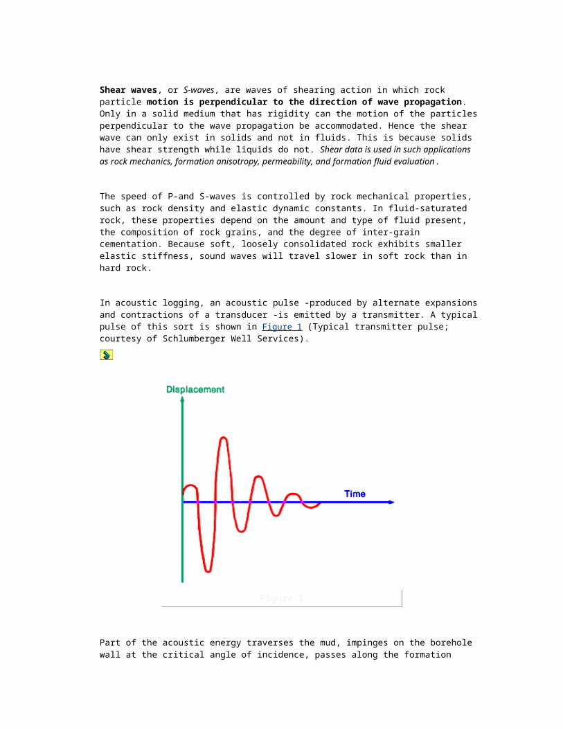
Figure 2

The volume of rock investigated by BHGM surveys is a function of the spacing between stations. Short spacing measurements investigate small rock volumes, longer measurements larger volumes. Figure   3 illustrates this concept.

Figure 3

If measurements are made at the top and bottom of a slab of formation 100 ft thick, 90% of the measured G effect will come from within an annulus round the borehole of 500 ft radius. For a 30 ft station difference, the 90% response is from within a

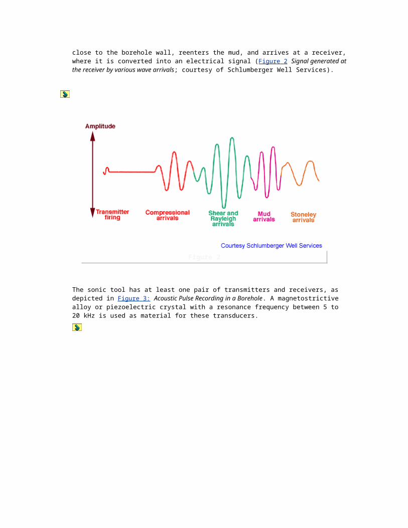
radius of 150 ft. A rough rule of thumb is that the BHGM "reads out" to five times the spacing between stations.

At all events the tool investigates a very large volume of rock compared to a conventional formation density tool, which reads a few inches at most into the formation.

There are currently two main applications for the BHGM:

obtaining formation density in completed wells not logged with a modern logging suite

detecting lithology, porosity, and fluid changes in the formation some distance from the borehole

An example of the first application is the detection of gas zones in an old well that has only an electric log. At the time these wells were logged and completed, gas production was not an economic proposition. Now that it is, the question remains of how to distinguish high-resistivity zones seen on the old ES log that are gas-bearing from low-porosity tight zones that have the same high resistivity. A BHGM survey can determine formation density over 10 to 20 ft intervals. Gas-bearing zones are likely to show densities closer to 2.0 gm/cc than the 2.5 gm/cc or more shown in tight zones.

An example of the second application is the detection of better porosity or gas some distance from an otherwise dry well. (The BHGM has been particularly successful in the Niagaran Reef plays in Michigan.) If the density distant from the borehole is calculated to be less than the density indicated by the conventional density log, then the well may be fractured over the more attractive gas-bearing or higher porosity zones.

Two tools are commercially available. They are the vibrating string type and the Lacoste-Romberg zero-length spring type. The Lacoste-Romberg device is the one used most frequently, due to its superior accuracy, repeatability, and temperature rating. Figure   4 illustrates the principal components of this device.

Figure 4

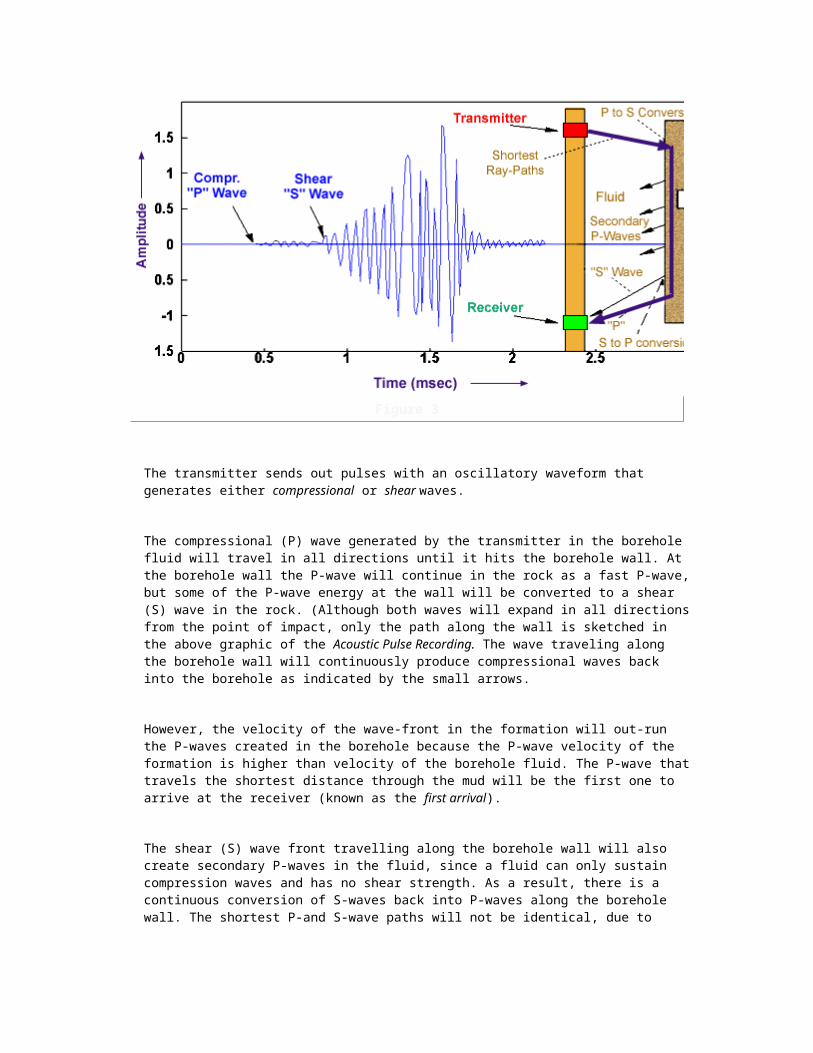
Figure   5 illustrates both an electric log and BHGM survey in a Gulf Coast Miocene sand/shale series.

Figure 5

Of interest are the two high-resistivity kicks seen at 2735-2750 ft and 2765-2780 ft. Either could be hydrocarbon-bearing or tight. The BHGM survey successfully predicted gas production from the upper sand from the calculated density of 2.08 gm/cc in contrast to the 2.38 gm/cc density in the lower sand. The well was perforated in the upper sand for an absolute open-flow potential (AOF) of 1.7 MMscf/D.

Figure   6 illustrates a carbonate well in which a featureless zone (6732-6750 ft) on the formation-density-compensated (FDC)

Figure 6

log was successfully completed for 1.5 MMscf/D because of the disparity between the BHGM density of 2.58 gm/cc and the FDC density of 2.72 gm/cc.

Borehole Televiewer (BHTV)

The BHTV is an acoustic device that scans the surface of the wellbore or casing by rotating an acoustic source (transducer) in the horizontal plane while the tool is moved vertically along the wellbore axis ( Figure   1 ). The amplitude and/or travel time of the acoustic signal reflected from the borehole or casing wall is displayed as a photograph of the section logged.

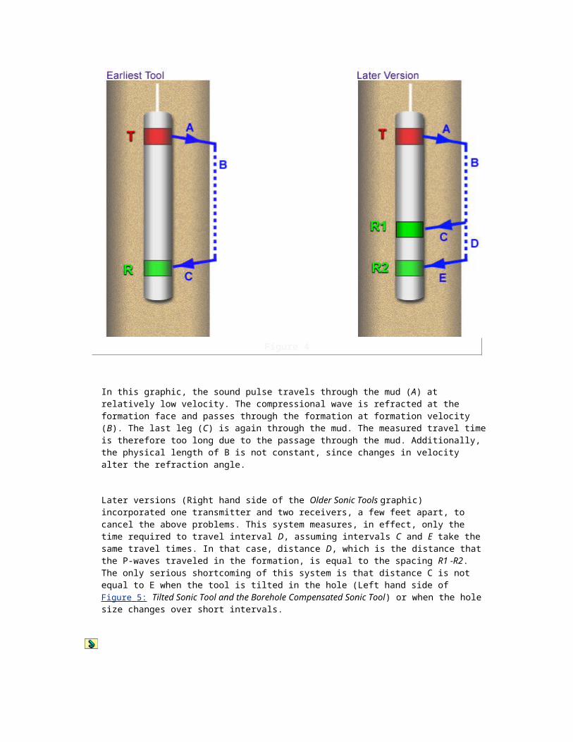
Figure 1

With the help of a flux gate compass, an oriented acoustic picture of the inside of the wellbore is provided as if it were split vertically along the north axis and laid flat.

The acoustic picture is presented in shades of gray and is a record of the amount of acoustic energy reflected from the borehole wall. A smooth surface reflects better than a rough one, a hard surface better than a soft, and a normal surface produces larger reflections than an oblique or slanted surface.

When a smooth, normal borehole wall is scanned, maximum energy is reflected, and the resulting image is a series of bright lines. However, when a feature such as a fracture with its attendant discontinuities is surveyed, a minimum amount of energy is reflected, and the feature appears as a dark line (dark represents reduced reflected energy).

In addition to fractures, features such as vugs, bedding planes, and changes in lithology, as well as perforations, ruptures, or pits in casing can be seen on the televiewer log.

In openhole, the BHTV is used to detect and measure the dip of fractures and bedding planes. Figure   2 is an isometric sketch of a wellbore intersected by a nonvertical fracture or bedding plane and a corresponding BHTV log.

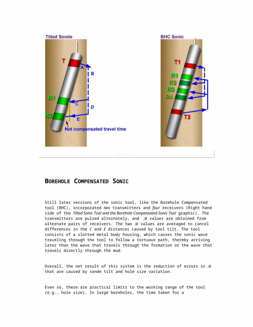
Figure 2

To determine dip, one merely finds the minimum of the sinusoid (indicated by the arrow) and reads the direction from the azimuth scale at the bottom of the log. Dip angle is determined by measuring the peak-to-peak amplitude, h, of the sinusoid and combining it with the diameter, d, of the wellbore:

dip angle = tan-1(h/d)Figure   3 is a view of a high-angle fracture or bedding plane intersecting the wellbore with north dip.

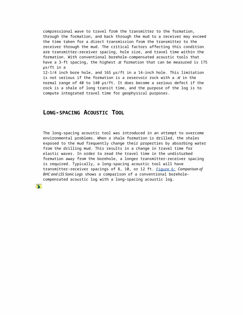
Figure 3

If a high-angle fracture intersects the wellbore with west dip, the BHTV anomaly is a full sine wave with a minimum to the west and a maximum peak occurring to the east, as shown in Figure   4 .

Figure 4

In the case of a fracture or bedding plane dipping to the east, the minimum would be to the east and the maximum to the west.

Figure   5 is an isometric view of a vertical fracture intersecting the wellbore in an east-west direction and a corresponding BHTV log.

Figure 5

The fracture appears as two vertical dark lines 1800 apart.

In a cased hole the BHTV may be used to detect perforations ( Figure   6 ),

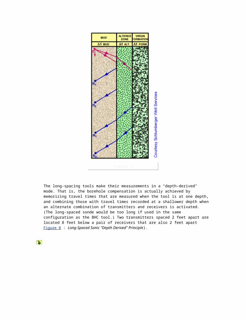
Figure 6

or evaluate damaged casing ( Figure   7 ).

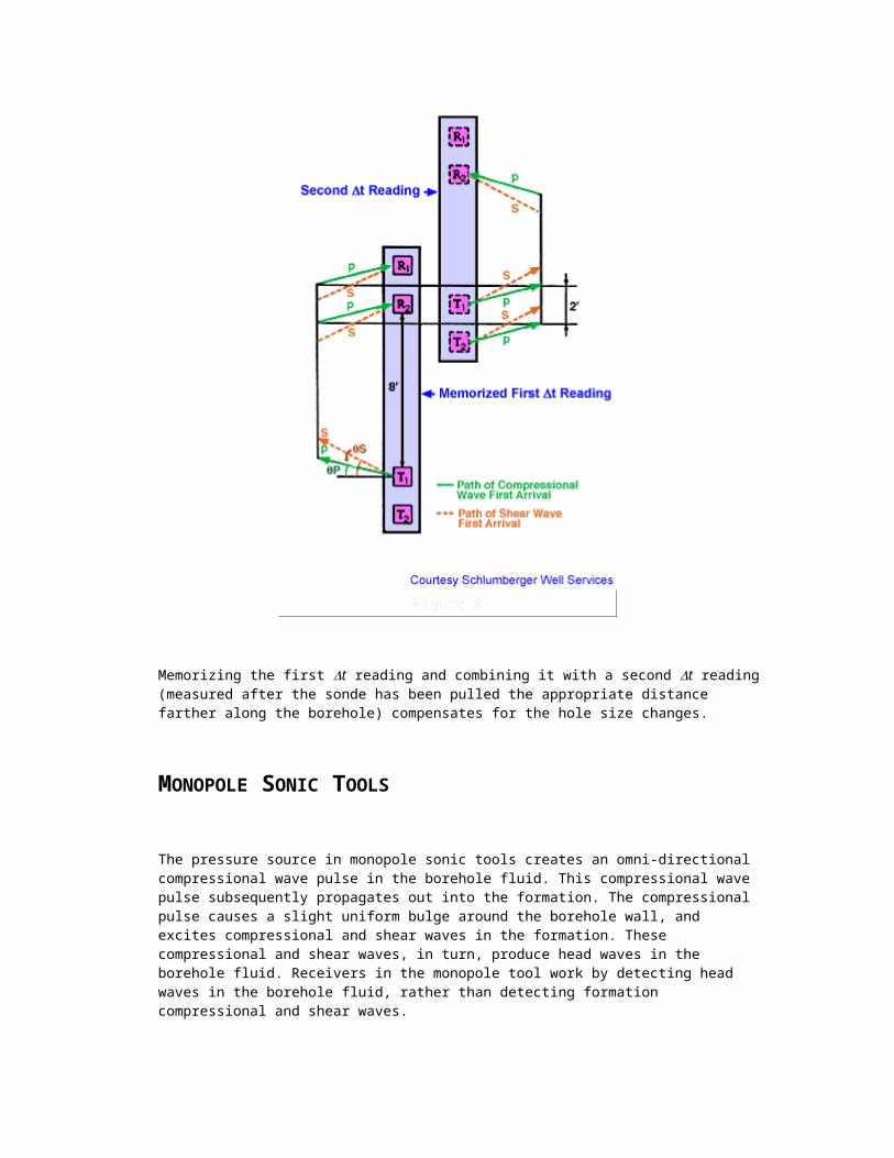
Figure 7

The BHTV can be run in any gas-free liquid such as fresh water, saturated brine, crude oil, or drilling mud. Operating limits for various mud weights and hole sizes may be determined from published charts.

Prerequisites for a top-quality log are a centered tool in a round hole. The log shown in Figure   8 meets these requirements.

Figure  8

There is a dark area on the left side of the log caused by the tool being slightly off center. Otherwise, the symmetrical intensity from left to right indicates a centered tool in a round hole.

Cased Hole LogsPulsed Neutron Logs

A pulsed neutron log provides a means of evaluating a formation after the well has been cased. It is of particular value for

evaluating old wells, where the original openhole logs are inadequate or nonexistent

monitoring reservoir performance over an extended period of time

monitoring the progress of the secondary and tertiary recovery projects

evaluating the formation, as a last resort, should the drillpipe become stuck

It is the most widely used and most direct logging method in cased holes at the present time. Other nuclear measurements are being developed that may eventually give superior results; these include the carbon/oxygen type logs and activation logs.

Though all commercially available tools are designed to measure the same formation parameters, their operating systems are all slightly different.

Principle of Measurement Regardless of the tool used, the principle of measurement remains the same. When a neutron generator is turned on for a very short period of time, a "burst" of neutrons leaves the tool. Since neutrons can easily pass through both the steel housing of the tool and the tubing/ casing, a "cloud" of neutrons gathers in the formation. Fast neutrons soon become "thermalized" by collisions with atoms in the formation. The most effective thermalizing agent is the hydrogen present in the pore space in the form of water or hydrocarbon. Once in the thermal state, a neutron is liable to be captured. The capture process depends on the capture cross section of the formation. In general, chlorine dominates the capture process. Since chlorine is present in formation water in the form of salt (NaCl), the ability of the formation to capture thermal neutrons reflects the salt content and, hence, the water saturation. The capturing of a thermal neutron by a chlorine atom gives rise to a capture gamma ray. Pulsed neutron tools therefore monitor these capture gamma rays. Thus, the common elements of all commercial pulsed neutron tools are a pulsed neutron generator and two gamma ray detectors at different distances from the neutron generator. Figure   1 illustrates a generalized neutron tool.

Figure 1

The cloud of neutrons produced by the initial neutron generator burst results in a cloud of thermal neutrons in the vicinity of the tool, which dies away as the neutrons are captured by chlorine atoms or other neutron absorbers in the formation. If there is plenty of chlorine present (i.e., high water saturation), the cloud of thermal neutrons disappears quite quickly. If, however, hydrocarbons are present (i.e., low water saturation), the cloud of thermal neutrons decays much more slowly.

The rate of decay is measured by monitoring how many capture gamma rays enter the gamma ray counter(s) as a function of time. Figure   2 plots the relative counting rate on the y-axis, and time, in microseconds, following the initial burst of fast neutrons, on the x-axis.

Figure 2

Note that after a few hundred microseconds a straight-line portion of the decay curve develops. Note also how the water line has a steeper slope than the oil line. At later times note the background gamma ray count rate that remains substantially constant.

The y-axis in Figure   2 is logarithmic but the x-axis (time scale) is linear. Thus, the straight-line portions represent exponential decay. If N is the number of gamma rays observed at time t and No is the number observed at t = 0, then

N = No et/

where r is the time constant of the decay process. is measured in units of time. It is convenient to quote values of in microseconds (1 microsecond = l0-6 seconds). The capture cross section of the formation, the property of interest, is directly related to by the equation:

S = 4550/where S is the capture cross section measured in capture units (CU).

Thus S is best measured by finding the straight-line portion of the capture gamma ray decay, and measuring its slope. This is accomplished in different ways by various commercially available tools.

On a typical pulsed neutron log as many as 9 curves may be displayed. Figure   3

Figure 3

illustrates a typical presentation:  

Curve Name Units Logs Track Remarks

Sigma (S) CU 2 & 3 Main curve

Tau ( ) µ-sec 2 & 3  

Ratio - 2 Pseudoporosity

Near Counts cps 3 Near detector, gate 1

Far Counts cps 3 Far detector, gate 1

Monitor or Background

cps 1 Near detector, gate 3

Quality Control - 1 Check of 7 loop

Gamma Ray API 1 Natural gamma

Casing Collar Log

- 1 Both memorized and direct

The Sigma Curve The S curve, the principal pulsed neutron measurement, behaves rather like an openhole resistivity curve; i.e., it deflects to the left (high values of S in wet zones and to the right (low values of S in hydrocarbon-bearing zones or low-porosity formations.

Since S values in shales are quite high, they tend to mask the effect of hydrocarbons, making shaly pay zones at first appear to be water-bearing. Figure   4 is a comparison of S with resistivity.

Figure 4

The Tau Curve is just another way of looking at S. In fact, is the basic measurement of the tool (the decay time constant for the thermal neutron population). However, all interpretation equations for pulsed neutron logs are linear functions of S. Thus, it is much easier to work with S than with . It is recommended that be recorded on tape but left of f the log presentation, since its scaled reciprocal (S) gives exactly the same information in a form that is easier to work with.

Ratio Curve The ratio curve is a porosity indicator derived by taking the ratio of gamma ray counts seen during gate 1 at the near and far detectors. The ratio curve, behaving very much like a compensated neutron porosity curve, deflects to the right (low ratio) in low porosity or in the presence of gas. Figure   5 shows the ratio curve response to a pocket of gas trapped below a packer behind a tubing nipple.

Figure 5

In the absence of any openhole porosity logs, the ratio can be used in combination with S to find formation porosity.

Near and Far Count-Rate Display In track 3 the near and far count rates are displayed as an overlay ( Figure   6 ). When the correct scales are chosen for the near and far count rate displays, the result is a useful "quick-look" log with the following properties:

in gas Fl > Nl (dotted left of solid)

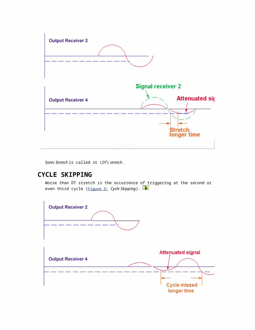
Figure 6

in shales Fl < Nl (dotted right of solid)

and in clean oil- or water-bearing zones, the two curves lie practically on top of one another.

Background and Quality Curves The background curve is a very insensitive natural gamma ray curve. Little movement shows on this curve except in "hot" zones, which are very radioactive. This curve is sometimes omitted without any great loss.

To summarize, the most important curves to work with are:  

S for water saturation

Ratio for porosity

GR for shale content

Near/far display for gas indications

 

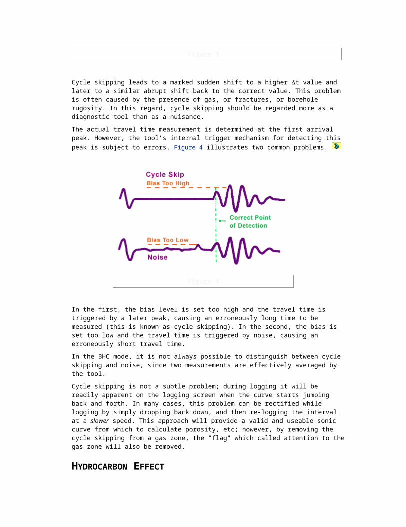
Capture Cross Sections

The capture cross section of a formation depends on the chemical elements present, and on their relative abundance. S values vary over a wide range.

Common matrix materials (sand, lime, and dolomite) exhibit capture cross sections in the range of 8 to 12 CU. Pore-filling fluids such as water, oil, and gas also show a wide range, brines varying from 22 CU (fresh water) up to 120 CU (saturated brine). Oils, depending on the amount of dissolved gas they contain, range from 18 to 22 CU. Gases, depending on their gravity, temperature, and pressure, range from 4 to 12 CU.

Interpretation of Pulsed Neutron Logs Practical interpretation of pulsed neutron logs in clean formations is conceptually very simple. The total formation capture cross section (S) recorded on the log, is the sum of the products of the volume fractions found in the formation and their respective capture cross sections. Thus, in its simplest form:

S log = S matrix • (1 -) + S fluid • Figure   1 should clarify the mathematical relationship.

Figure 1

If the "fluid" is a mixture of oil and water, the log response is described by S log =S ma (1 -) + S w Sw + S hy (1 - Sw)

By rearrangement of the equation, we have

Reservoir Monitoring-Time Lapse Technique Pulse neutron logs are useful for monitoring the depletion of a reservoir. The time lapse method is used. A base log is run in the well shortly after initial completion but before substantial depletion of the producing horizons. A few days, weeks, or even months of production are required to "clean up" near-wellbore effects of the drilling operation, such as mud filtrate invasion. Once a base log is obtained, the well may be relogged at time intervals over the life of the field, depending on production rate variations.

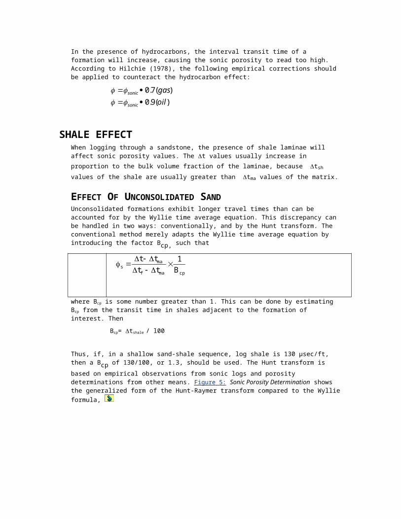
Successive logs may be overlaid so that changes in saturation can be easily spotted by changes in S. A good example of this ( Figure   2 ) shows a base log and three additional logs at roughly six-month intervals. Note the rapid rise of the oil-water contact(s) with passage of time.

Figure 2

Log-Inject-Log The log-inject-log technique is used to find residual oil saturations. Once a base log is run, the formation is injected with waters of different salinities and logged again. In Figure   3 , the formation was injected with brine and logged, then injected with seawater and logged a third time.

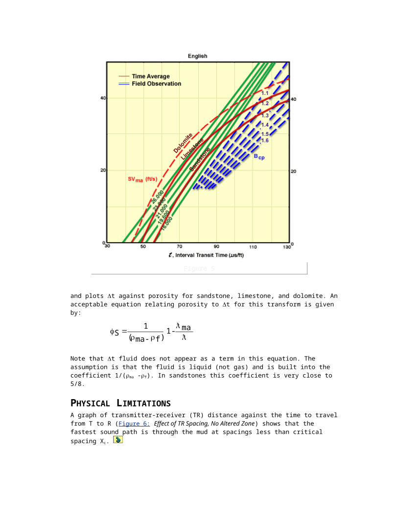
Figure 3

Provided the capture cross section of the seawater and brine flushes are known, all the unknown quantities may be normalized out and the residual oil saturation found, using

Note that it is not necessary to know either Sma or SoilThe technique has many variations, some using specially chlorinated oil that has a high capture cross section.

Inelastic Neutron-Gamma (Carbon-Oxygen) Logs

High-energy neutrons (14 Mev) produced by a pulsed-neutron source are directed into the formation, and the energy spectrum of gamma rays produced by the neutron bombardment is sampled at various times both during and after the neutron burst. Neutrons can interact with matter in two distinct ways to create gamma rays: by inelastic scattering with nuclei at high energies (>5 Mev) and, through capture or absorption, by nuclei at low energies (<.025 Mev). The gamma rays produced from each of these reactions have unique energies that depend on the type of nucleus with which the neutron reacts. By measuring the number and energy of gamma rays

produced by neutron bombardment, the elemental composition of the formation can be inferred.

Applications These tools provide a measure of the oil saturation, C/O ratio; lithology, Si/(Ca + Si) ratio; porosity, H/(Ca + Si) ratio; shale, Fe/(Ca + Si) ratio; and salinity, Cl/H ratio, in open or cased holes. This logging method is used to determine the presence of hydrocarbons behind casing, regard-less of formation water salinity.

At present, reliable measurements can be made only with optimum borehole and formation conditions. The major interpretive uncertainty stems from the inability of the measurement to distinguish between carbon associated with carbonates (e.g., limestone, CaCO3) and carbon associated with hydrocarbons.

Depending on the tool used, the tool either (a) measures the number of gamma rays in two energy "windows," centered around the expected carbon and oxygen inelastic scattering energies during the burst and around the silicon and calcium thermal capture energies after the burst, or (b) employs a "spectral fitting analysis" to determine the yields of carbon, oxygen, calcium, silicon, and several other elements. This spectral fitting analysis uses three gates: the burst gate, the background gate, and the capture gate. The burst gate is at the source, the background gate cuts down on borehole interference, and the capture gate gives capture readings. The burst gate minus the background gate gives the inelastic spectrum and the capture gate gives the capture spectrum ( Figure   1 ).

Figure 1

Ratios of element yields (C/O, Si/Ca, Cl/H, etc.) are normally presented. Given a constant porosity and lithology, an increase in the carbon-oxygen ratio indicates an increase in oil saturation. It should be noted that by taking elemental ratios, any variations in neutron output from the source are normalized.

Note the following considerations:

The log is generally run in cased holes when conditions are not favorable for pulsed neutron logs because of low formation water salinities. Optimum formation conditions are high porosity (>20%), low water salinity (<50,000 ppm NaCl), and consistent or known lithology. The log can be useful where salinities are unknown or variable. Depth of investigation is very shallow for measurements on the inelastic scattering spectrum. This limits the tool’s openhole use and forces consideration of the effects from the casing annulus. Optimum borehole conditions are a small-diameter hole and constant fluid composition in the casing. If an oil-water contact or varying salinities are expected in the casing, a fluid displacer should be considered. At present, the statistical uncertainty in analyzing the spectrum is the tool’s limiting feature. Advances in detector design and spectrum analysis should solve these problems.

Figure   2 shows a continuous carbon/oxygen log.

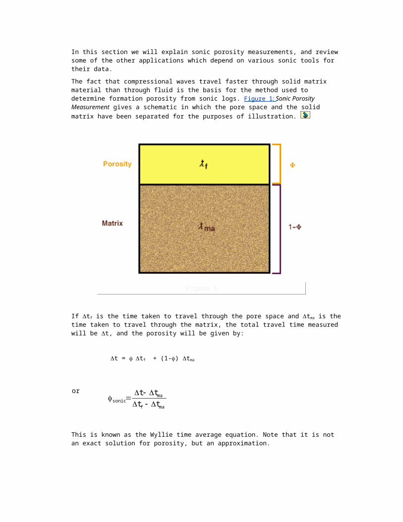
Figure 2

The curves it presents are:   Track 1 Monitor

  Silicon correlation

Tracks 2 and 3  Silicon-calcium ratio (capturespectrum)Carbon-oxygen ratio Calcium-silicon ratio (inelastic spectrum) 

Figure   3 shows an inelastic neutron gamma log of the sort that employs spectral filtering.

Figure 3

The data it records are:  

Track 1 Ion-Indicating ratio Fe/(Si+Ca) Porosity indicating ratio

(H/(Si+Ca)

   Tracks 2 and 3 

Lithology indicator (Si/(Si+Ca)  Carbon/oxygen ratio (C/O)  Salinity indicator (Cl/H) 

 

Casing Inspection Logs

Casing Inspection Logs

Inspection of the mechanical state of the completion string is an important aspect of production logging. Many production (or injection) problems can be traced back to mechanical damage to, or corrosion of, the completion string. A number of inspection methods are available, including

· multifingered caliper logs

· electrical potential logs

· electromagnetic devices

· borehole televiewers or borehole TV

The majority of these devices measure the extent to which corrosion has taken place. Only the electrical potential logs indicate where corrosion is currently taking place. With the exception of the caliper logs, all the devices require that the tubing be pulled before running the survey, since most methods are designed to inspect casing rather than tubing, and most employ large-diameter tools.

Caliper Logs

Various arrangements of caliper mechanisms are available to gauge the internal shape of a casing or tubing string. Figure   1 illustrates three such tools.

Figure 1

Tubing profile calipers determine the extent of wear and corrosion and detect holes in the tubing string--all in a single run into the well. The large number of feelers on each size of caliper ensures detection of even very small irregularities in the tubing wall.

In pumping wells, the tubing caliper log may be run by one person, not a whole pulling unit crew. A "pull sheet" showing the maximum percentage of wall loss of every joint of tubing in the well may be prepared. Before the well is pulled, a program of rearranging the tubing string can be provided. Moving partially worn joints nearer the surface and discarding thin-wall joints substantially prolongs the effective life of tubing strings and reduces pulling costs in pumping wells. In flowing or gas lift wells, the tubing profile caliper provides an economical method of periodically checking for corrosion damage, monitoring the effectiveness of a corrosion inhibitor program, or detecting and removing damaged tubing joints when "working over" a well.

One accessory tool that may be run in combination with the tubing profile caliper is a split detector. This tool, functioning much like a magnetic collar locator, is designed to detect and log vertical splits or hairline cracks in the tubing that might be difficult to locate with the profile caliper. In practice, the split detector is used to log down the

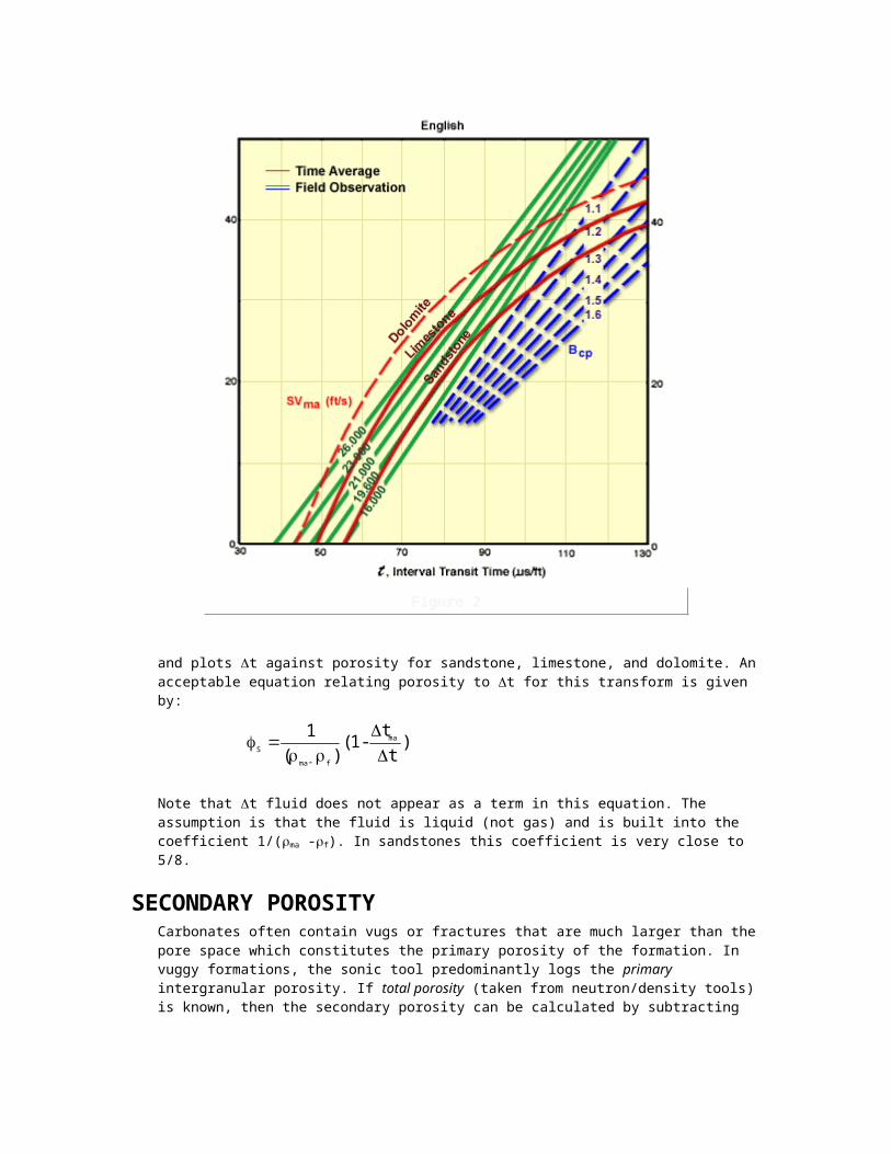
tubing, and the profile caliper to log up the tubing. This gives a complete inspection for wall thickness and splits in one run of the cable in the well.

Casing profile calipers, which log 4 1/2-in. through 20-in. OD casing, are especially valuable where drilling operations have been carried on for an extended period of time through a string of casing. The determination of casing wear is of great importance when deciding if a liner can be safely hung, or if a full production string is required. In producing wells, the casing profile caliper will locate holes or areas of corrosion that may require remedial work. The tool is also valuable when abandoning wells because it permits grading of casing to be salvaged before it is pulled.

Electrical Potential Lags

An electrical potential log determines the galvanic current flow entering or leaving the casing.

This indicates not only where corrosion is taking place and the amount of iron being lost, but also where cathodic protection will be effective. The magnitude and direction of the current inside and outside the casing is derived mathematically from electrical potential measurements made at fixed intervals throughout the casing string. In order to achieve reliable results from this kind of survey, the borehole fluid must be an electrical insulator; i.e., the hole must either be empty or filled with oil or gas. Mud or other aqueous solutions cause a "short" that invalidates the measurements. The log itself is a recording versus depth of the small galvanic voltages detected. Figure   1 illustrates such a log, showing three runs, for each of which a different cathodic protection voltage was applied to the casing string.

Figure 1

Figure   2

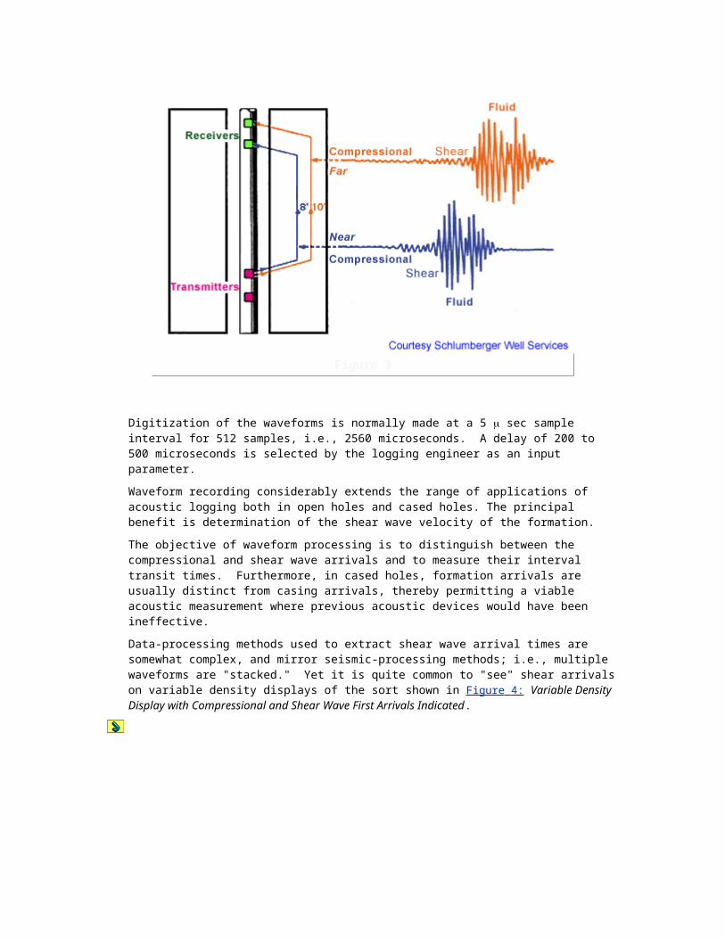
Figure 2

and Figure   3 show an interpretation of casing potential profile logs run both with and without cathodic protection.

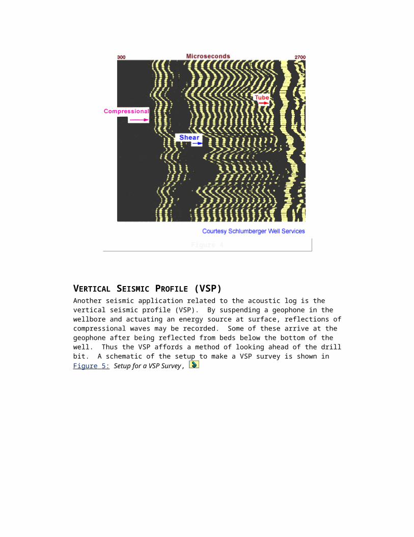
Figure 3

Note that in Figure 3 the metal loss has been reduced to practically zero by application of an appropriate cathodic protection.

Electromagnetic Devices

The most commonly used casing corrosion inspection tools are of the electromagnetic type. They come in two versions: those that attempt to measure the remaining metal thickness in a casing string, and those that try to detect defects in the inner or outer wall of the casing.

They operate in a manner similar to openhole-induction tools. Each consists of a transmitter coil and a receiver coil. An alternating current is sent through the transmitter coil. This sets up an alternating magnetic field that interacts both with the casing and the receiver coil ( Figure   1 ).

Figure  1

The coils are spaced about three casing diameters apart to ensure that the flux lines sensed by the receiver coil are those that have passed through the casing.

The signal induced in the receiver coil will be out of phase with the transmitted signal. In general, the phase difference is controlled by the thickness of the casing wall. Thus, the raw log measurement is one of phase lag in degrees and the log is scaled in degrees. Figure   2 illustrates an ETT log in severely corroded casing.

Figure 2

Note that an increasing thickness corresponds to an increase in the phase shift angle. Some presentations of this log show a rescaling in terms of actual pipe thickness. This requires that the operator make some calibration readings in the type of casing present in the well. It is common to see large differences in thickness between adjacent stands due to a number of variables, such as the drift diameter of the pipe, the weight/foot, and the magnetic relative permeability of the steel used.

Another closely related measurement uses a slightly different technique and forms the basis of the pipe analysis log (PAL), also known as the vertilog. Two electromagnetic measurements are of interest in the context of the pipe analysis tool: magnetic flux leakage and eddy current distortion.

If the poles of a magnet are positioned near a sheet of steel, magnetic flux will flow through the sheet ( Figure   3 ).

Figure 3

As long as the metal has no flaws the flux lines will be parallel to the surface. However, at the location of a cavity, either on the surface of the sheet or inside it, the uniform flux pattern will be distorted. The flux lines will move away from the surface of the steel at the location of the anomaly, an effect known as flux leakage. The amount of flux distortion will depend upon the size of the defect. If a coil is moved at a constant speed along the direction of magnetic flux parallel to the metal sheet, a voltage will be induced in the coil as it passes through the area of flux leakage.

The larger the anomaly, the greater the flux leakage, and therefore the greater the voltage. The magnetic flux is distorted on both faces of the sheet, regardless of the location of the defect, and therefore the coil only needs to be moved along one surface to survey the sheet completely. As the coil must be moved through a changing magnetic flux to produce a voltage, no signal is generated when it is moved parallel to the surface of an undamaged sheet of steel.

When a relatively high frequency alternating current is applied to a coil close to a sheet of steel, the resulting magnetic field induces eddy currents in the steel ( Figure   4 ).

Figure 4

These eddy currents in turn produce a magnetic field that tends to cancel the original field, and the total magnetic field is the vector sum of the two fields. A measure voltage would be induced in a sensor coil situated in the magnetic field. The generation of eddy currents is, at relatively high frequencies, a near-surface effect, so if the surface of the steel adjacent to the coil is damaged, the magnitude of the eddy currents will be reduced and, consequently, the total magnetic field will be increased. This will result in a variation in the sensor coil voltage. A flaw in the sheet of metal on the surface away from the coils will not be detected and, depending upon its distance from the surface, a cavity within the sheet will not influence the eddy currents either.

The measuring sonde of the pipe analysis tool consists of an iron core with the pole pieces of an electromagnet at each end, and twelve sensor pads in two arrays between the pole pieces ( Figure   5 ).

Figure 5

The two arrays are juxtaposed to ensure complete coverage of the inner surface of the casing. Each of the pads contains a transmitting coil for the eddy current measurement, and two sensor coils wound in opposite directions for both the flux leakage and eddy current measurements. The two sensor coils are wound in opposite directions so that for both measurements there is zero voltage so long as no anomaly exists, but a signal will be produced when the quality of the casing is different below the two coils. The same sensor coils can be used for both measurements, as two distinct frequencies are involved. A frequency of 2 kHz is used for the eddy cur-rent measurement, giving a depth of investigation of about 1 mm. The sensor pads are mounted on springs so that they are held in contact with the casing, facilitated through centralization of the sonde. Various sizes of magnet pole pieces are available and are selected according to the inside diameter of the casing (casing ID) to optimize the signal strength for the flux leakage measurement.

Six measurements of flux leakage and eddy current distortion are made on each array, and the maximum signal from each array is sent uphole to the surface instrumentation. Four signals are recorded, both eddy current and flux leakage data from the two arrays.

The flux leakage data correspond to anomalies located anywhere in the casing, while eddy current distortion only occurs at the inside wall of the casing. The standard

presentation of the measurements is as shown in Figure   6 , with the data from the two arrays displayed in tracks 2 and 3.

Figure 6

Enhanced data are displayed in track 1, making any anomalies more obvious. At any particular depth the larger of the two flux leakage readings is selected and held for about 0.3 seconds on the display; the same is done for the eddy current data. This enhancement only occurs if the signal amplitudes exceed a certain threshold, to ensure that only significant defects are made more apparent. The holding of the signal allows signal levels to be seen more clearly.

Cement Bond Logging

This variant of acoustic logging makes use of the observation that on acoustic logs run inside casing with good cement bonding, the amplitude of the signal detected at the receiver is much reduced, while in unsupported casing the signal remains strong. The log format may include a gamma ray and casing collar log for depth control, a transit-time curve, and an amplitude measurement for evaluation of bonding. There may also be a "signature" or a "variable density" display of the actual waveforms. These displays aid both quality control and log evaluation. In Figure   1 , a typical

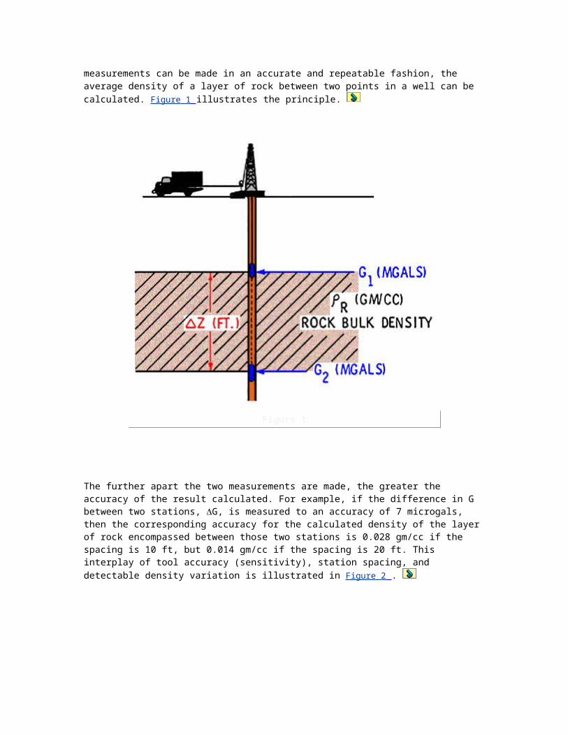
cement bond log presentation, GR and casing collar logs are omitted.

Figure 1

Measurement Principle A cement sheath bonded to the casing can be intuitively predicted to attenuate sound propagation in the pipe. CBL tools are able to differentiate between "no cement" and "solid cement." In the in-between range, however, these tools are not yet able to provide unambiguous answers to the question, Will the cement job prevent high-pressure fluid flow in the annulus? Even so, the tool is a valuable and much-used adjunct to completion work.

Cement bond logs began as auxiliaries to the acoustic log, run with tools designed for D-type logging. The information supplied was important enough to motivate development of special CBL tools, which now do the majority of the bond-logging measurements.

The chief problem with acoustic-type CBL tools is that the casing-signal attenuation is not directly related to the degree of hydraulic sealing provided by the annular cement. Hence, no matter how accurately the attenuation is measured, answers are still in terms of probabilities, except in the extreme conditions of perfect or no bonding.

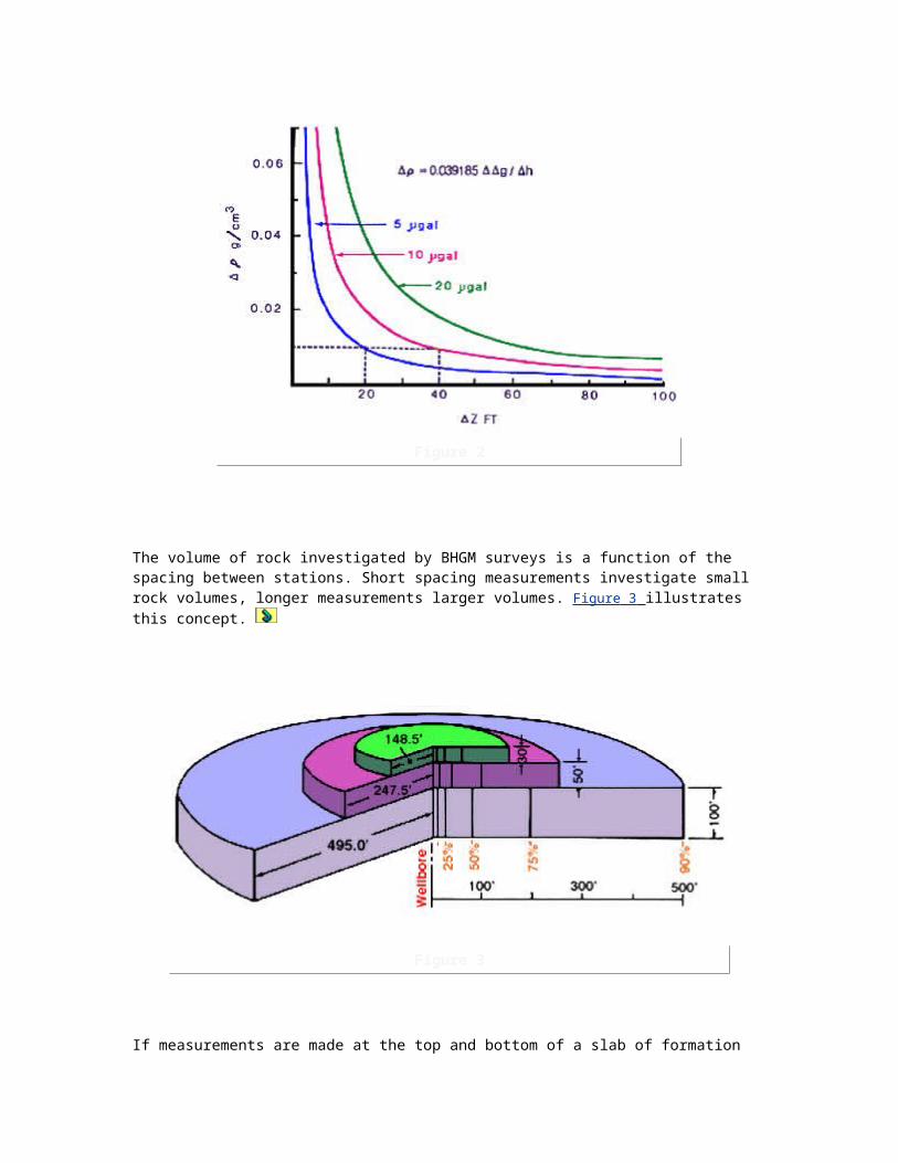
Figure   2 illustrates the interplay of cement presence, bonding, signature, variable density display, and amplitude.

Figure 2

A CBL log should always include a section above the presumed cement top, where the pipe is completely unbonded. This gives one endpoint for the log; the amplitude curve should never read higher than this. The other endpoint is given by the zero point on the log scale. The curve never reads zero, but comes close (2-3 mv) in well-bonded pipe.

The paradox of acoustic-amplitude-type CBL logging is that the signal of most interest is zero or near it, but the equipment triggers on a finite signal in normal operating mode. As the signal approaches zero, it gets harder and harder to fine-tune the system to pick up the right signal. To correct this, the more sophisticated tools allow a detection window set at a selected time interval after the first pulse. This time is normally close to the casing transit time.

As with normal interval transit time logging, good quality control with the CBL requires the use of an oscilloscope picture. With most equipment, this is the only way to be sure that the amplitude measurement is made on the first-arriving half-cycle of acoustic energy, essential for meaningful interpretation. Figure   3 illustrates this concept.

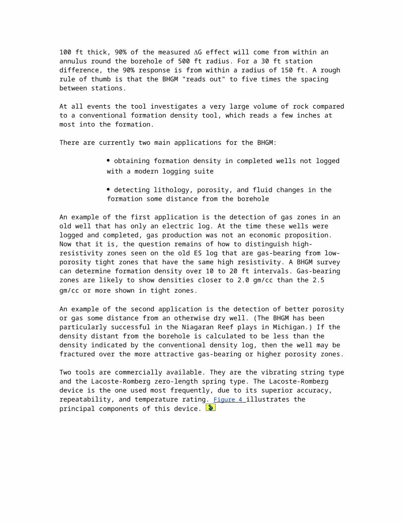
Figure  3

In normal logging mode, the system triggers on the first arriving (El) half-cycle, measuring both its single-receiver travel time (time from transmitter to receiver) and its amplitude. Two things can prevent this: (1) weak signals in well-bonded pipe can go below the detection threshold and (2) in hard-rock country, it is possible for formation signals to arrive ahead of casing signals. In the first case, cycle skips appear on the log ( Figure   4 ), and the amplitudes recorded in the "skip" intervals are not interpretable.

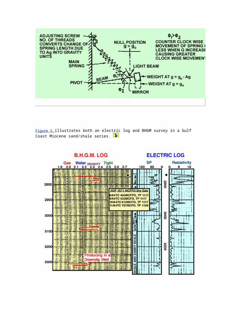
Figure  4

In the second case, the transit-time curve departs from the fairly straight-line value of casing transit time, and begins to follow formation variations. The scale is not directly correlatable, since the CBL transit time is a 3-ft single-receiver measurement and is not borehole-compensated. Normal casing transit time is 3 ft X 57 µsec/ft plus the travel time from tool to casing and back again, usually around 250-260 µ sec.

Most CBL tools assume in-phase arrivals through all sides of the casing, meaning that the tool must be centered. The degree of centering can be judged from the transit-time curve. A poorly centered tool produces shorter transit times. Centering may be virtually impossible in deviated holes or large casings.

Borehole Televiewer

Tools with TV capability are available for borehole scanning.

The oldest is the borehole televiewer (BHTV), which uses a rotating ultrasonic transmitter and receiver to produce an image of the borehole or casing. There is also a borehole television camera that uses a TV camera and an intense light source to transmit a visual image of the borehole wall to the surface ( Figure   1 ).

Figure  1

The borehole television camera records on videotape and can be viewed with conventional video playback equipment.

 

 Production Logs

Production Logs

Production Logs fit into three categories: profile logging, fluid identification, and temperature logging.

Profile Logging Profile logging may be used to monitor injection rates in injection wells, to monitor production rates in producing wells, or to detect casing, tubing, and/or packer leaks, and channeling behind pipe in poorly cemented zones.

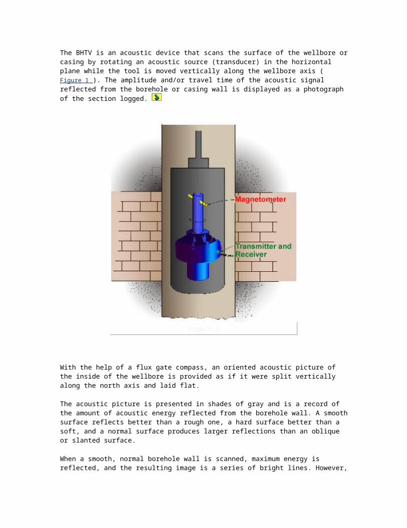
Although some tools can handle both environments, there are some methods applicable only to injection profiling.

In general, profiles may be obtained without disturbing dynamic well behavior by using the proper pressure control equipment and operating techniques; i.e., logs can, and should, be run through tubing without having to kill the well or pull the tubing.

Before attempting to obtain a profile log, plan the operation in advance with the logging service company, paying particular attention to:

expected flow rate

casing and tubing size, type, and weight

expected wellhead pressure

type of Christmas tree connections

tubing restrictions

corrosive or poisonous production fluids

completion records

openhole logs

Profiling tools available for measurement of fluid flow rates fall into three major categories: continuous flowmeters

packer or restrictor type flowmeters

radioactive tracers (velocity and tracer modes)

Figure   1 ,

Figure 1

Figure   2 ,

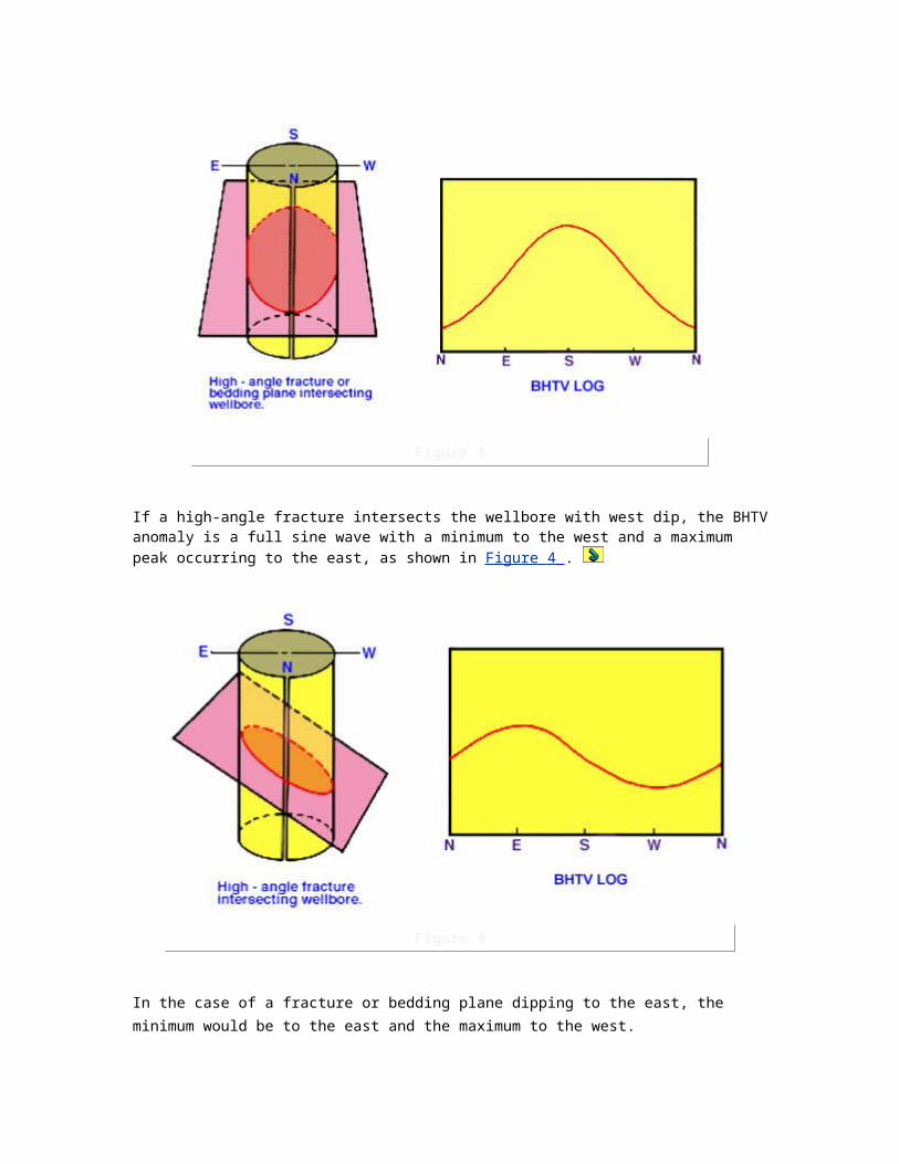
Figure 2

and Figure   3 illustrate the three types of flowmeter--the packer,

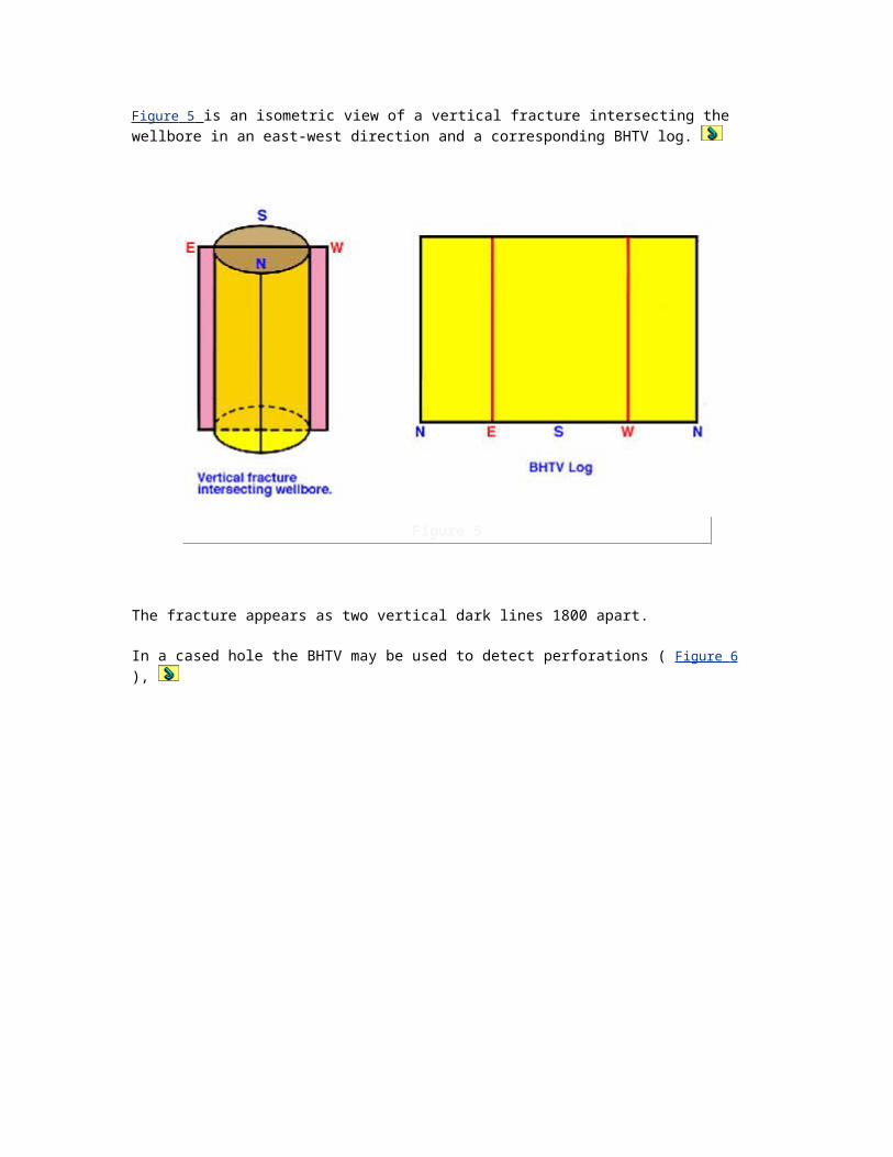
Figure 3

the continuous, and the fullbore; Figure   4 illustrates a radioactive tracer tool.

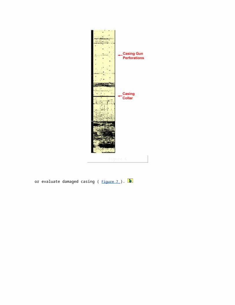
Figure 4

The accuracy of fluid flow rate measurements depends on:

the number of commingled phases

the well deviation

the type of tool and the way it is run

hole diameter variations

production/injection rate variations

Greater confidence in results can be expected when there is only one phase flowing (oil or water or gas), when the well is vertical, and when the appropriate tool is used for the particular well conditions. A lesser degree of confidence can be placed in results in deviated wells, conditions producing froth or slug flow, in wells that are "heading," and where the design limitations of the tools are exceeded (e.g., continuous flow-meters in low flow rate wells). For safety reasons, radioactive tracer surveys should only be run in injection wells.

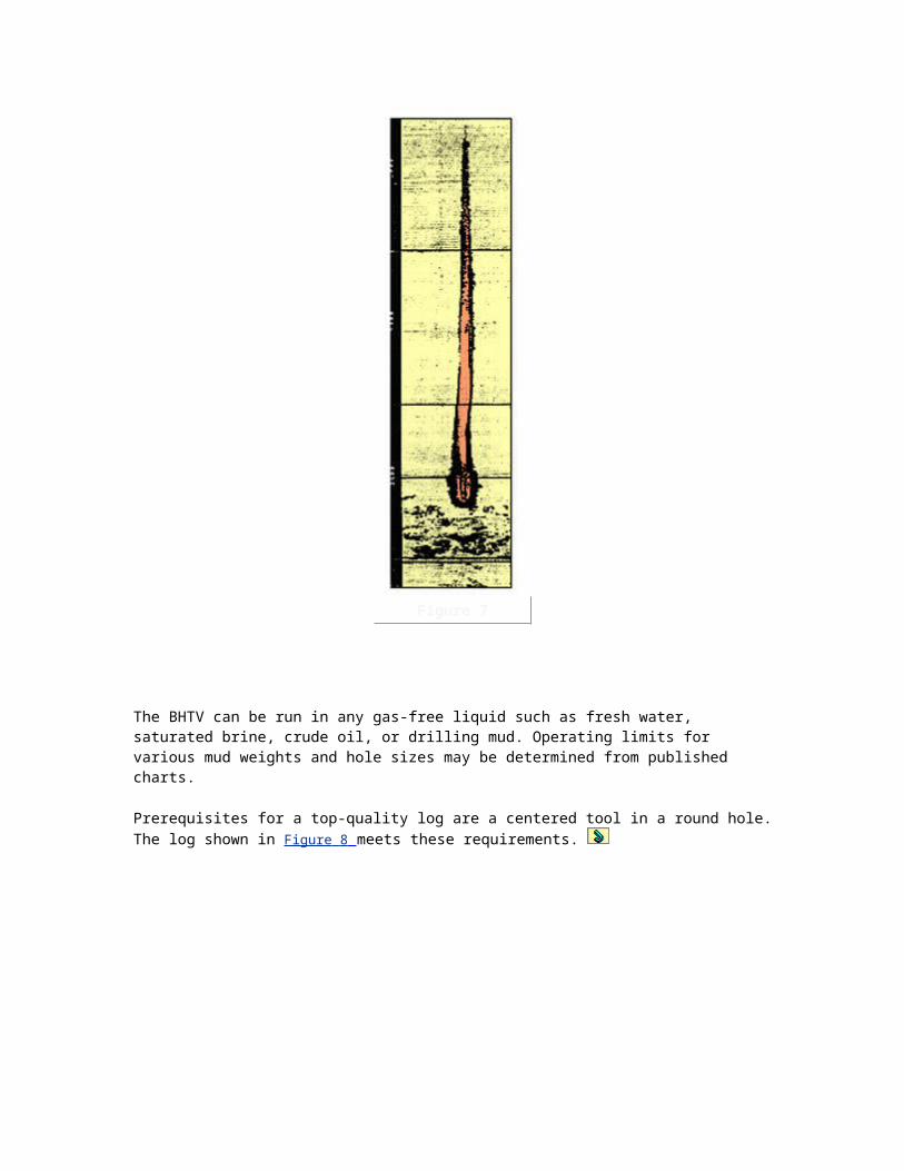
Figure   5 shows a production profile made from a flowmeter survey.

Figure 5

Figure   6 shows a radioactive tracer survey made in a "time-lapse" mode.

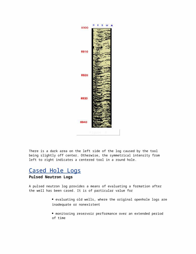
Figure 6

Note the final destination of the released tracer material.

Fluid Identification

Production logging tools that can differentiate between oil, gas, and water in a producing well allow diagnosis of a number of completion problems, better understanding of reservoir performance, and monitoring of secondary and tertiary recovery projects.

In particular, they help to pinpoint gas, oil, and water entries into, and exits from, the production string, as well as to determine, in combination with flow measurements, how much of which fluid is produced from which horizon.

Many tools are available to distinguish one type of fluid from another. Their functions are measurement of fluid density, measurement of fluid dielectric constant, recovery of a fluid sample at well flowing pressure, and measurement of frequency spectrum of noise generated by fluid flow.

Two commonly used devices are:

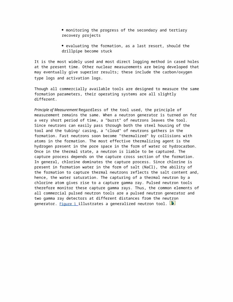
the gradiomanometer ( Figure   1 ), which measures the pressure difference in the wellbore between two pressure sensors a fixed distance apart

Figure 1

the fluid density log ( Figure   2 ),

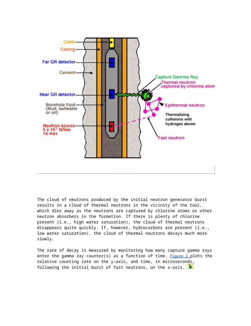
Figure 2

which measures the absorption of gamma rays by the fluid between a gamma ray source and a detector

The hydro log ( Figure   3 ) measures the dielectric constant of the fluid flowing in the wellbore. Because of the large difference between the dielectric constant of oil and water, the holdup of the flowing mixture may be estimated.

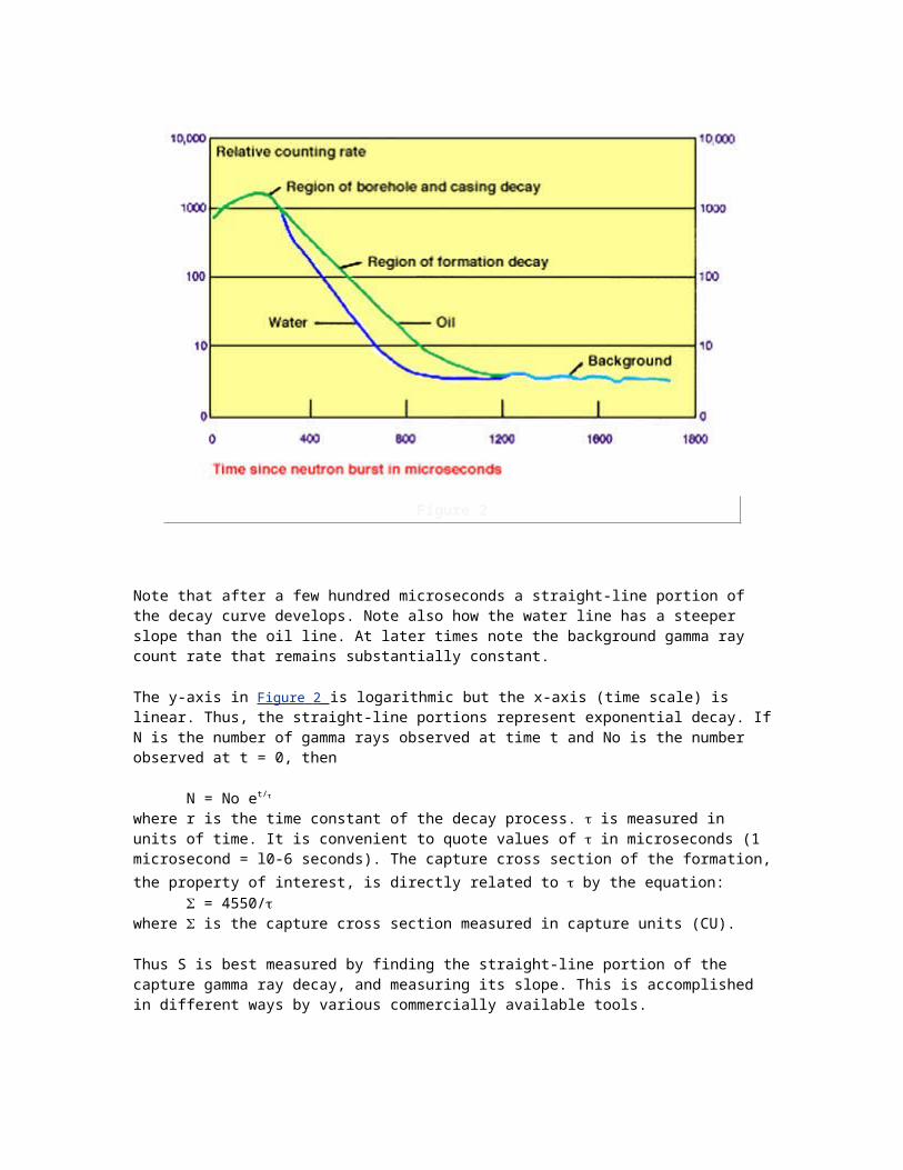
Figure  3

Figure   4 illustrates a downhole fluid sampler.

Figure 4

This instrument may be used to retrieve a sample of fluid from the well. It is useful for collecting oil, water, and gas samples for PVT analysis and pinpointing fluid levels in a well.

Turbulent fluid movement generates noise. Both the amplitude and frequency of this noise vary with the quantity and type of fluid and the medium through which the fluid is flowing. Measurements of these characteristic sounds can be interpreted to indicate the type of fluid flow and its location. In the case of gas, it is possible to calculate the approximate rate of flow.

TEMPERATURE LOGGINGTemperature logs may be used to monitor fluid flow in production or injection wells; they have the added advantage of detecting fluid flow outside the completion string in tubing/casing annulus or casing/formation annulus. They are particularly useful for finding gas entries to, or exits from, the wellbore; channels in poorly cemented sections; lost circulation zones in openhole; and the cement top in a recently cemented well.

Three types of temperature measurements are commonly available: a conventional temperature survey, a differential temperature survey, and a radial differential temperature survey.

Figure   1 illustrates a conventional thermometer and associated temperature survey.

Figure 1

Figure   2 illustrates the radial differential thermometer and its associated survey,

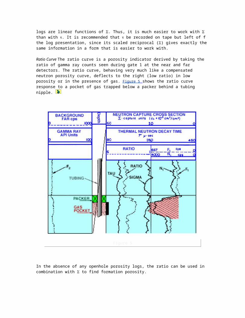
Figure 2

in connection with which the operator should

choose an appropriate scale so that there are no excessive scale changes over the zone of interest

log going down where possible so that the presence of the tool and cable in the wellbore does not influence the measurement being made

remember that temperature-measuring devices are normally quite sensitive to temperature changes, but not very accurate in absolute terms

Figure   3 illustrates a temperature log showing oil production through a perforated interval.

Figure 3

Sampling & Testing

Sidewall Coring Devices

The objectives of coring are to bring a sample of the formation and its pore fluids to the surface in an unaltered state, to preserve the sample, and to transport it to a laboratory for analysis.

These objectives are hard to meet since the very act of cutting a core will, to some extent, alter both the properties of the rock itself and the saturation of the fluids in its pores.

A number of techniques exist for minimizing the damage to formation samples. Other techniques, aimed at restoring the original state of the formation sample when it was at reservoir conditions, may also be brought into play at the time the core is analyzed.

Two methods of retrieving formation samples using wireline tools are currently in use: the conventional sidewall core gun, and a relatively new device, the core plugger.

Sidewall Cores Figure   1 illustrates a sidewall core gun; Figure   2 shows it in close-up.

Figure 1

The body of the gun carries a number of hollow steel bullets that can be fired selectively into the formation by means of explosive charges.

Figure 2

Once lodged in the formation, the bullet can be retrieved by means of attached flexible steel wires. By raising the gun in the borehole, the tension on the wires is usually increased sufficiently to dislodge the bullet.

Once samples have been collected, the gun is raised to the surface and each core plug stored in a glass jar marked with the well name and the depth from which it was cut. Subsequently, these cores may be analyzed for porosity, permeability, and hydrocarbon content.

Note that the gun is equipped with an SP electrode. This allows the tool to be placed at the correct depth in the well prior to sampling by correlation of a short section of the Sp log with other openhole logs already run.

These guns come in a variety of shapes and sizes. On average, they are capable of retrieving 60 samples in one trip into the hole. The diameter of the core barrel may be anywhere between 3/4 in. and 1 1/8 in. The length of the core retrieved is a function of many variables. Depending on the strength of the explosive charge used, the type of core barrel selected, and the hardness of the formation, the length of the recovered sample may be as long as 2 in., or as short as nothing at all.

There are obvious limitations to the amount of data that can be obtained from sidewall cores. In the first place, the sample is taken from a part of the formation that has been flushed with mud filtrate. Secondly, the act of explosively firing the coring bullet into the formation may induce local fracturing. Occasionally, the retainer wires

used to retrieve the core barrel may sever and the bullet will be lost in the hole. Lastly, the trip up the hole to the surface involves a considerable amount of flushing through the mud column. Despite these drawbacks, sidewall cores are still good quick-look indicators of formation properties. It is normal practice to inspect these cores at the wellsite for hydrocarbon odor, fluorescence, stain, and cut if a mud logging unit or geologist’s doghouse is available.

Core Plugger The core plugger uses a motorized circular bit to bore into the wall of the formation in order to retrieve samples. Currently, this tool is capable of cutting up to 12 core samples in one run in the hole. Core size is 15/16 in. in diameter and 1 3/4 in. long. Each core takes about five minutes to cut. This device works better than the conventional sidewall core gun in consolidated formations, and causes no physical damage to the sample.

Wireline Formation Testers

Wireline formation testers serve a number of useful purposes, including obtaining a sample of formation fluid, gauging formation permeability, and measuring formation pressure to determine formation pressure gradients.

Wireline formation testers have been used for many years to recover samples of formation fluid both in open and cased holes. Traditional tools suffered from a number of drawbacks, such as lack of resolution and accuracy of pressure gauges, and the inability of the instrumentation to tell the operator whether or not a good packer seal was obtained until it was too late to rectify the situation.

These inadequacies have now largely been overcome by the introduction of two key features of modern repeat formation testers, namely quartz crystal pressure gauges and pretest capabilities that allow the operator to rectify a bad seal before it leads to undesirable results. An added bonus is the ability of these tools to make pressure tests independent of sample taking. Indeed, in practice nowadays it is quite common to use these tools solely to make pressure tests.

Tool Characteristics and Applications Most service companies now offer a repeat formation tester that includes pretest chambers, sample chambers, and a high-resolution pressure gauge.

Wireline formation testers are particularly useful

when investigating zones of interest in which conventional tests are not feasible, such as those too far above TD, those lacking good intervals for setting straddle packers, or those with very short intervals, where depth control is critical

for pinning down water-oil, gas-oil, or gas-water contacts

when rig time is critical

when pressure control is critical because of time of day or rig locations

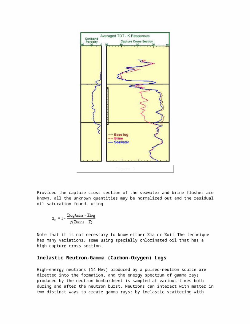
When ordering the service, give plenty of notice to the service company. Variables such as sample size, packer hardness, choke size, pressure gauges, and water cushions may not be universally available. If a sample of recovered hydrocarbons is needed for PVT lab analysis, a special pressure cylinder should be requested.

When running the tool, a valid test is one that recovers significant quantities of fluid and/or records formation and hydrostatic pressure.

A dry test is indeterminate, and the tool should be repositioned several times to determine whether the formation is impermeable (in which case all tests will be dry) or the tool was set in a shale or tight streak (in which case repositioning should result in a valid test).

A lost packer seal is also indeterminate. In that case, the tool should be repositioned. Openhole logs are particularly helpful in resolving dry tests and lost packer seals. The microlog, if available, is useful as an indicator of tight streaks, and caliper logs, particularly the four-arm type, are useful for avoiding hole conditions leading to lost packer seals.

Operating Principles Figure   1 shows the RFT tool in the closed position (a) for descending into the well, and in the open (set) position (b) for pressure measurement and sample taking.

Figure 1

Communication between the formation and the tool interior is established through the probe. Figure   2 is a schematic of the tool’s sampling system.

Figure  2

Note the details of the actuation of the filter probe: in the setting cycle it is forced to cut through mudcake, and in the sampling cycle it is retracted to open the path for formation fluids.

Note also the pretest chambers and the position of the sample chambers. The two pretest chambers, automatically activated every time the tool is set, withdraw 10 cc of formation fluid each. Chamber 2 has a higher flow rate than chamber 1. The actual rates of fluid withdrawal vary with the tool and the downhole conditions but are approximately 50 cc/min for chamber 1 and 125 cc/min for chamber 2, resulting in pretest times of roughly 12 seconds and 5 seconds. The pretest samples are expelled back into the mud column and are not saved.

Figure   3 shows a typical log produced during a test.

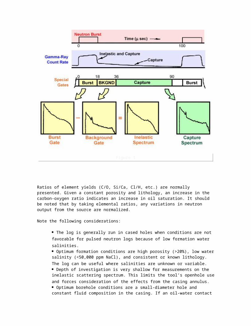
Figure 3

Since the tool is stationary in the hole during the test, the recording is made on a time scale with increasing time in the down-hole direction on the log. Notice that in track 1, pressure is recorded in analog form. Four subtracks record the units, tens, hundreds, and thousands of psi.

Each record shows the following pressures:

before tool is set--hydrostatic during pretest--drawdown after pretest--buildup after buildup--formation pressure

The standard gauge used in the RFT is a strain gauge calibrated by a "dead weight" tester. The accuracy of this system, after applying temperature corrections, is 0.41% of full scale, i.e., 41 psi for a 10,000 psi gauge. The resolution of the gauge is about I psi, with a repeatability of 3 psi. The accuracy may be improved to 0.31% full scale if a special calibration technique is employed involving placement of the gauge and the downhole electronics in a temperature-controlled oven.

Where greater accuracy is required, a high-precision quartz gauge may be used. The accuracy is then 0.5 psi, provided that the temperature is known within 1° C. Resolution is on the order of 0.01 psi.

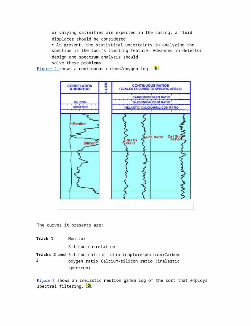
It should be noted ( Figure   4 ) that the quartz gauge is located lower in the tool than the reference measurement point that is the strain gauge. Hence, the pressure recorded by the two gauges is different due to the hydrostatic head of a column of silicone grease.

Figure 4

In some cases, a further pressure difference may be noted between the two gauges, since the strain gauge is calibrated in psig and the quartz gauge is psia.

Interpretation In order to make the greatest use of RFT data, the analyst should be able to interpret the following types of RFT records:

pretest records for formation permeability

post pretest buildup for formation permeability

large-sample fill-up time for formation permeability

sequential pressure readings versus depth for pore pressure gradients

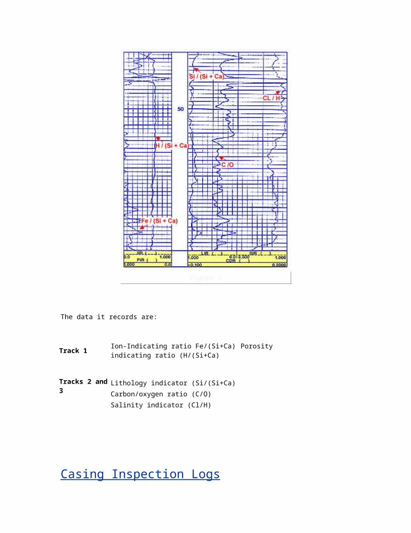
large-sample collection data for expected formation product ion

Pretest Records for Formation Permeability Figure   5 shows a typical pretest record.

Figure 5

In reality, only one pretest is required to estimate formation permeability. The magnitude of the pressure differential (P) between pretest sampling pressure and formation pressure coupled with the flow rate during pretest is sufficient to define permeability. In general, this may be found by a relation of the form

k = A • C • q • µ / Pwhere:

k is permeability in millidarcies

A is constant to take care of units

C is the flow shape factor

q is the flow rate in cc/second

µ is the viscosity of the fluid in cp

P is the drawdown in psi

A number of flow regimes may exist around an RFT tool and the borehole. It is generally agreed that the flow is somewhere between hemispherical and spherical. Computer modeling of the probe/formation system for one service company’s tool shows that the combination of constants A • C to be used should be such that

The flow rate is derived by dividing the 10 cc volume of the pretest chamber by the sampling time read from the pressure record. The viscosity, µ is considered to be that of the mud filtrate and may be estimated from published charts. P is read from the pressure recording as the difference between pretest sampling pressure and formation pressure.

The pretest method of permeability determination has these limitations:

If the permeability is very high, the drawdown is very small and cannot be measured accurately.

If the permeability is very low, the sampling pressure may drop below the bubble-point, in which case gas or water vapor is liberated and the

flow rate of the liquid withdrawn is less than the volumetric displacement rate of the pretest pistons.

The volume of formation investigated is small and hence the permeability measured may be that of the damaged zone, if present, and thus not representative of the formation as a whole.

In general, a good estimate of formation permeability may be obtained from a visual inspection of the pretest record.

Post Pretest Buildup for Formation Permeability Permeabilities obtained from pretest may be subject to the errors mentioned above; they also may not be measuring absolute permeability but the relative permeability to the water in the flushed zone. Figure   6 marks the pretest region on a set of relative permeability curves, from which it can be deduced that the pretest permeabilities are less than half absolute permeability when measured in an invaded oil zone.

Figure  6

A preferred method of calculating permeability is the analysis of the late-time portion of the pressure buildup record after the pretest disturbance has been made. A much larger rock volume can be investigated in this fashion. The method effectively measures kro close to Swirr, very close to k absolute (see Figure   6 ) when the measurement is made above the transition zone.

Figures 7a and 7b illustrate two modes of propagation of a pressure disturbance; Figure   7a is for spherical propagation and Figure   7b for cylindrical propagation.

Figure 7a

In a thin bed, the cylindrical mode predominates, whereas in a thick bed the spherical mode prevails.

Figure  7b

In order to determine whether cylindrical or spherical flow is predominant in a test, the pressure may be plotted against one of two time functions, respectively derived on the assumption of cylindrical and spherical flow. The characteristics of these time functions are such that a plot of pressure versus the relevant time function for the actual flow regime involved produces a straight line whose slope is proportional to the formation permeability and whose intercept at the zero time point gives the formation pressure. Figure   8 gives an example of such time-pressure plots.

Figure  8

Large-Sample Fill-Up Time for Formation Permeability When a large sample of formation fluid is recovered, the time taken to fill the sample chamber can be used as an indicator of permeability. Drawdown is here considered to be the formation pressure itself, since the sample chamber is for all practical purposes at atmospheric pressure. This may not hold true if the fill-up time is limited by a water cushion and a choke. Use this method with discretion and take it for what it is: a quick and dirty way of finding permeability.

For one service company’s large sample chamber, the following equation may be used:

where: k is fill-up permeability in mud

C is flow-shape factor

q is flow rate in cc/sec

µ is fluid viscosity in cp

P is drawdown pressure in psi

Sequential Pressure Readings versus Depth for Pore Pressure Gradients Since many formation pressure measurements may be made on one trip in the hole, pressure gradients can be calculated and plotted. The easiest method is to plot formation pressure against depth. It is useful to plot hydrostatic pressure on the same plot.

Gas-oil and oil-water contacts are evident on a plot of this nature. The fluid density can be deduced from the pressure gradient, by using

fluid density gm/cc = pressure gradient (psi/ft) • 2.3072Care should be taken in low-porosity transition zones where capillary pressure effects are pronounced. Log-derived oil-water contacts (OWC), for example, may appear somewhat shallower in the well than the free water level indicated from plots of formation pressure versus depth.

Formation Production Estimates When a large sample is recovered, it is possible to predict formation productivity by analysis of the recovered oil, water, and gas. At the surface a miniseparator is used to measure the volumes of oil, water, and gas recovered ( Figure   9 ). The water recovered will be a mixture of mud filtrate and formation water. The amount of formation water is calculated from the relationship:

Figure 9

% 

Empirical charts then link recovered volumes to predicted production. Three areas are delineated on the chart indicating formations that are gas, oil, and water productive. An estimate of water cut can also be made using: