wetland monitoring and assessment program for
TRANSCRIPT

OFFICIAL‐Sensitive
Arthur Rylah Institute for Environmental Research Technical Report Series No. 322
Wetland Monitoring and Assessment Program for
environmental water Stage 3 Final Report
P. Papas, R. Hale, F. Amtstaetter, P. Clunie, D. Rogers, G. Brown, J. Brooks, G. Cornell,
K. Stamation, J. Downe, L. Vivian, A. Sparrow, D. Frood, M. West, D. Purdey, L. Sim, E. Bayes, L. Caffrey, B. Clarke-Wood and L. Plenderleith
March 2021

Acknowledgment
We acknowledge and respect Victorian Traditional Owners as the original custodians of Victoria's land and waters, their unique ability to care for Country and deep spiritual connection to it. We honour Elders past and present whose knowledge and wisdom has ensured the continuation of culture and traditional practices.
We are committed to genuinely partner, and meaningfully engage, with Victoria's Traditional Owners and Aboriginal communities to support the protection of Country, the maintenance of spiritual and cultural practices and their broader aspirations in the 21st century and beyond.
Arthur Rylah Institute for Environmental Research Department of Environment, Land, Water and Planning PO Box 137 Heidelberg, Victoria 3084 Phone (03) 9450 8600 Website: www.ari.vic.gov.au
Citation: Papas, P., Hale, R., Amtstaetter, F., Clunie, P., Rogers, D., Brown, G, Brooks, J., Cornell, G., Stamation, K., Downe, J., Vivian, L., Sparrow, A., Frood, D., Sim, L., West, M., Purdey, D., Bayes, E., Caffrey, L., Clarke-Wood, B. and Plenderleith, L. (2021). Wetland Monitoring and Assessment Program for environmental water: Stage 3 Final Report. Arthur Rylah Institute for Environmental Research Technical Report Series No. 322. Department of Environment, Land, Water and Planning, Heidelberg, Victoria.
Front cover photo: Kinnairds Wetland (west), Geoff Brown
© The State of Victoria Department of Environment, Land, Water and Planning 2021
This work is licensed under a Creative Commons Attribution 3.0 Australia licence. You are free to re-use the work under that licence, on the condition that you credit the State of Victoria as author. The licence does not apply to any images, photographs or branding, including the Victorian Coat of Arms, the Victorian Government logo, the Department of Environment, Land, Water and Planning logo and the Arthur Rylah Institute logo. To view a copy of this licence, visit http://creativecommons.org/licenses/by/3.0/au/deed.en
Edited by Jeanette Birtles (Organic Editing) and John Birtles (Birtles Tech Editing).
ISSN 1835-3827 (print) ISSN 1835-3835 (pdf)) ISBN 978-1-76105-368-9 (print) ISBN 978-1-76105-368-9 (pdf)
Disclaimer This publication may be of assistance to you but the State of Victoria and its employees do not guarantee that the publication is without flaw of any kind or is wholly appropriate for your particular purposes and therefore disclaims all liability for any error, loss or other consequence which may arise from you relying on any information in this publication.
Accessibility If you would like to receive this publication in an alternative format, please telephone the DELWP Customer Service Centre on 136 186, email [email protected] or contact us via the National Relay Service on 133 677 or www.relayservice.com.au. This document is also available on the internet at www.delwp.vic.gov.au
Arthur Rylah Institute for Environmental Research Department of Environment, Land, Water and Planning Heidelberg, Victoria
Wetland Monitoring and Assessment Program for environmental water Stage 3 Final Report
Phil Papas1, Rob Hale1, Frank Amtstaetter1, Pam Clunie1, Danny Rogers1, Geoff Brown1, Jacqui Brooks2, Gabriel Cornell1, Kasey Stamation1, Judy Downe1, Lyndsey Vivian1, Ashley Sparrow1, Doug Frood3, Lien Sim4, Matt West5, Daniel Purdey1, Elaine Bayes6, Laura Caffrey2, Bradley Clarke-Wood7 and Lynette Plenderleith8
1Arthur Rylah Institute for Environmental Research 123 Brown Street, Heidelberg, Victoria 3084
2Water and Catchments Division, Department of Environment, Land, Water and Planning 8 Nicholson Street, East Melbourne, Victoria 3000
3Doug Frood, Pathway Bushlands and Environment, Marraweeney, Victoria 3669
4Lien Sim, Cape Woolami, Victoria 3925
5Matt West, School of Biosciences, University of Melbourne, Parkville, Victoria 3010
6Elaine Bayes, Rakali Ecological Consulting, Chewton, Victoria 3451
7Bradley Clarke-Wood, BirdLife Australia, 60 Leicester Street, Carlton, Victoria 3053
8Lynette Plenderleith, Frogs Victoria, St Albans, Victoria 3021
Date
Arthur Rylah Institute for Environmental Research Technical Report Series No. 322, Department of Environment, Land, Water and Planning
WetMAP Stage 3 Final Report
ii
Acknowledgements This project was funded by the Water and Catchments Group, Department of Environment, Land, Water and Planning (DELWP), as part of the Victorian Government’s $222M investment to improve the health of waterways and catchments under Water for Victoria.
For contributions to field work and data compilation, we thank Zak Atkins, Peter Fairbrother, Annique Harris, Lauren Johnson, Chris Jones, Matt Jones, Jason Lieschke, Annette Muir, Mike Nicol, Patrick Pickett, Andrew Pickworth, Jo Sharley, Daniel Stoessel, Arn Tolsma (all ARI), Kate Bennetts (Fire Flood & Flora), Darren Quinn (BirdLife Australia), Peter Brown, Michelle Casanova (Charophyte Services), Damien Cook (Rakali Ecological Consulting), Steve Davidson, Jeff Davies, Guy Dutson, Will Honybun (North Central CMA), Dylan Osler, Julian Smith, Simon Starr and Rustem Upton. BirdLife Australia provided access to their waterbird count databases (facilitated by Chris Purnell) in addition to their field support. We thank Melbourne Water for their continuing and long-term support of waterbird monitoring at the Western Treatment Plant, and for making the results available for addressing wider issues in waterbird management.
We appreciate the input from the Catchment Management Authorities (CMAs), Parks Victoria and water authority staff who contributed their knowledge of local wetlands and environmental watering and helped facilitate site access, including: Emma Healy, Braeden Lampard, Kate McWhinney, Jennifer Munro, Malcolm Thompson and Jane White (Mallee CMA); Will Honybun, Kevin Mah, Louissa Rogers, Peter Rose, Amy Russell and Genevieve Smith (North Central CMA); Simon Casanelia, Jo Deretic and Keith Ward (Goulburn Broken CMA); Saul Vermeeren, Sharon Blum-Caon and Jayden Wooley (Corangamite CMA); Catherine McInerney (North East CMA); Greg Fletcher (Wimmera CMA); Jacob Bergamin, Wayne Morgan, Kathryn Stanislawski and Leeza Wishart (Parks Victoria); Mick Dedini (DELWP); Sarah Binger (Goulburn Valley Water) and Brad Hutchison (Lower Murray Water).
We thank Emma Ai, Bex Dunn, Claire Krause and Leo Lymburner (Geoscience Australia) for guidance and provision of data for WetMAP sites from the Wetland Insights Tool. These data were used in our analyses of the Supplementary Questions. We thank David Weldrake (Murray–Darling Basin Authority) for provision of the hydrology data used to explore some Supplementary Questions by the bird theme. We thank Tina Hines (Monash University) for completing the chlorophyll analysis, and Christine Hall for sorting and identifying zooplankton for our bird and fish themes. The North Central CMA is thanked for providing salinity data for some wetlands and Daniel Stoessel (ARI) is thanked for providing insight into the management of Murray Hardyhead wetlands. Christine Arrowsmith (Australian UAV) is thanked for facilitating and collecting aerial imagery from some vegetation sites to inform an assessment of the extent of Tall Marsh vegetation.
We thank Pat Feehan (BirdLife Murray–Goulburn) for coordination of citizen science bird monitoring and all members of BirdLife Murray–Goulburn for their valuable contribution to the project. Paul Flemons, Jodi Rowley and Adam Woods from the Frog ID team at the Australian Museum are thanked for their collaboration and support with WetMAP’s frog citizen science program ‘Frogs are Calling You’.
We thank Lauren Johnson, Justin O’Connor, Michael Scroggie, Peter Menkhorst, Arn Tolsma, Claire Moxham Kaylene Morris (all ARI) and Claire Hollier (DELWP Waterway Programs) for their input on earlier drafts of the report, and we thank Neville Amos, Nick Clemann, Justin O’Connor, Tracey Regan, Ivor Stuart, Zeb Tonkin and Matt White (all ARI), Rob Clemens, Joris Driessen, Chris Purnell (BirdLife Australia), Iain Ellis (NSW Department of Primary Industries) and Clayton Sharpe (Charles Sturt University) for their valuable input into the program design. We also thank Tarmo Raadik, Peter Menkhorst, Fern Hames (ARI), Will Steele (Melbourne Water), Don Driscoll (Deakin University), Andrew Bennett (LaTrobe University), Andrew Greenfield (Mallee CMA), Geoff Heard (then, ARI), Chris Bloink, Steven Saddlier (Ecology Australia) and Teresa Mackintosh, for their valuable contributions to program planning.
We acknowledge the Independent Review Panel: Jane Catford (King’s College London), Paul Boon and Peter Vesk (The University of Melbourne), Nick Whiterod (Aquasave-NGT), Skye Wassens (Charles Sturt University) and Heather McGuinness (CSIRO); and the Project Steering Committee: Adrian Clements (WGCMA), Genevieve Smith (NCCMA), Emma Healy (MCMA), Mark Toomey (VEWH), Andrea White, Maegan Walker, Paul Reich and Terry Chan (DELWP).
The final draft of the report was compiled, edited and styled by Jeanette Birtles (Organic Editing) and John Birtles (Birtles Tech Editing).
We express thanks to landowners Ken and Jill Hooper (Wirra-Lo Wetland Complex) and managers Paul Lewis (Tahbilk Winery) and Colleen and Peter Barnes (Trust for Nature) for providing access to properties.
This study was completed under Victorian Flora and Fauna Guarantee Permit 10007273, DELWP Research Permit 10008640, Fisheries Victoria Research Permit RP-827, Animal Ethics Permits 15-05, 19-003 and 18-010 (DELWP Animal Ethics Committee) and a Parks Victoria permit issued through ParkConnect.
Field work was undertaken on the lands of the following Traditional Owners: Barapa Barapa, Dja Dja Wurrung, Jardwadjali, Nguraliliam Wurrung, Wadiwadi, Ladjiladji, Yorta Yorta and Watha Wurrung.

WetMAP Stage 3 Final Report
iii
Contents
Acknowledgements ii
Summary 1
1 Introduction 7
WetMAP Stages 1 and 2 7
WetMAP in the Victorian monitoring and reporting context 7
Program governance 8
Program objectives and themes 9
Stage 3 planning, monitoring questions and evaluation 9
Planning and commencement of monitoring 9
Revision of Key Evaluation Questions and development of Supplementary Questions 10
Monitoring sites 11
Control sites and counterfactuals 12
Informing adaptive management and CMA water management plans 12
Collaborations 12
Communication and engagement 13
References 14
2 Vegetation theme 15
Introduction 15
Wetland vegetation in Victoria 15
Responses of wetland vegetation to inundation 15
WetMAP vegetation monitoring questions: development and rationale 19
Methods 21
Study area and wetlands 21
Survey design 26
Survey methods 27
Data analysis 28
Results 35
Summary of vegetation characteristics among surveys and wetlands 35
Responses of understorey vegetation to inundation and environmental water (KEQs 1–3, SQ 1) 38
Response of lignum to inundation and environmental water 53
Response of trees to inundation and environmental water 55
Discussion 58
Understorey vegetation responses to environmental water 58
Response of lignum to environmental water (KEQ 4) and antecedent factors (SQ 4) 62
Response of tree tip growth and flowering to inundation and environmental water (KEQ 5) 63
Survival of mature trees (KEQ 6) 63
Conclusions and future directions 64
References 68

WetMAP Stage 3 Final Report
iv
3 Frog theme 74
Introduction 74
Key drivers of frog occurrence 74
Responses to environmental water 75
WetMAP frog monitoring focus and questions 76
Hypotheses 78
Efficacy of frog monitoring techniques 78
Methods 80
Study wetlands 80
Survey area 80
Frog survey techniques 80
Habitat and water quality assessment 84
Experimental design to test key evaluation questions 85
Analysis and modelling 86
Results 90
Frog occurrence/distribution 90
Do environmental water events increase abundance or species richness of frogs in wetlands? (KEQ 1 and KEQ 2) 92
Do environmental water events precipitate breeding by frogs in wetlands? (KEQ 3) 94
What survey technique or combination of techniques is the most effective in detecting the greatest number of frog species and measuring abundance in wetlands? (SQ 1) 94
Exploration of frog relationships with hydrological regimes (preliminary evaluation of KEQs 4–6, SQs 2–4) 99
Discussion 101
Response of frog abundance (KEQ1) and species richness (KEQ2) to environmental water 101
Response of frog breeding to environmental water (KEQ 3) 101
Determining the most effective survey methods to measure frog species richness and abundance (SQ 1) 102
Preliminary evaluation of longer-term KEQs and SQs 103
Conclusions and future directions 104
References 105
4 Bird theme 111
Introduction 111
Waterbird usage of wetlands 111
Benefits of environmental water to birds 112
Modifiers of bird responses to watering 114
Key Evaluation Questions and Supplementary Questions 115
SQ 1: How do waterbird abundance and species richness change with water level in watered wetlands? 116
SQ 2: How do waterbird abundance and species richness change with duration of flooding in watered wetlands? 117
SQ 3: How do waterbird abundance and species richness change with frequency of inundation of watered wetlands? 118
WetMAP Stage 3 Final Report
v
SQ 4. Are waterbird abundance and species richness affected by continental rainfall patterns and water availability in the Australian landscape? 119
Methods 120
Study area and wetland selection 120
Monitoring frequency and timing 123
Survey methods 123
Waterbird counts 123
Data collection – ProofSafe app 124
Evidence of breeding 124
Habitat classification and utilisation 124
Woodland birds 125
Water quality and zooplankton 126
Hydrological history 127
Statistical analysis 127
Results 133
KEQ 1: Do environmental water events increase the abundance and species richness of birds in wetlands? 133
KEQ2: Do environmental water events result in bird breeding at wetlands? 136
KEQ 3. Do environmental water events increase suitable habitat for foraging, roosting and breeding of waterbirds in wetlands? 137
KEQ 4. Do environmental water events increase the abundance and species richness of woodland birds adjacent to wetlands? 140
SQ1–SQ3 Exploration of bird relationships with hydrological regimes 141
SQ 4 Are waterbird abundance and species richness affected by continental rainfall patterns and water availability in the Australian landscape? 143
Discussion 149
Responses of waterbird abundance and species richness to environmental water events (KEQ 1) 149
Response of waterbird breeding to environmental water at wetlands (KEQ 2) 150
Changes in waterbird habitat following watering events (KEQ 3) 152
Responses of woodland birds adjacent to wetlands to environmental water events (KEQ 4) 152
Exploration of relationships with hydrological regimes (SQ 1–3) 153
Are waterbird abundance and species richness affected by continental rainfall patterns and water availability in the Australian landscape? (SQ 4) 154
Conclusions and future directions 156
Applied considerations for future research 156
Next steps 157
References 157
5 Fish theme 160
Introduction 160
Small-bodied generalist fishes 161
Murray Hardyhead 163
Key Evaluation Question and hypothesis development 163
General methods 167

WetMAP Stage 3 Final Report
vi
Study area 167
Sampling fish within wetlands 167
Zooplankton and chlorophyll a sample collection 172
Assessment of wetland size 172
Inundation extent and wetland productivity 174
Methods 174
Results 174
Discussion 176
Conclusions and future considerations 176
Wetland water regime 177
Methods 177
Results 177
Discussion 178
Conclusions and future considerations 179
Immigration and emigration of native fishes 180
Methods 180
Results 181
Discussion 184
Conclusions and future considerations 186
Monitoring the persistence of Murray Hardyhead 187
Methods 187
Results 188
Discussion 193
Conclusions and future directions 193
Overall discussion 194
Future considerations 194
References 195
6 Communication and engagement 200
Background 200
Approach 200
Key messages and target audiences 201
Activities and methods for engagement 202
Evaluation of communication and engagement 208
Communication and engagement outputs 208
Engagement outcomes 209
Highlights 210
Recommendations for Stage 4 210
Stage 4 Communication and Engagement Plan 210
Citizen science 211
The benefits of citizen science in ecological research and monitoring 211
Citizen science in Victorian Government 211
Pilot projects 212

WetMAP Stage 3 Final Report
vii
Project aims 212
Approach 213
WetMAP frog citizen science 214
WetMAP bird citizen science 216
Preliminary evaluation 218
Recommendations for WetMAP Stage 4 citizen science 218
References 219
7 Conclusion 221
Short-term environmental water outcomes (KEQs) 221
Filling knowledge gaps to inform management (SQs) 223
Key findings and management considerations 224
Vegetation 224
Frogs 224
Birds 224
Fish 225
Communication and engagement 226
References 226
Appendices 228
Appendix 1: Scoring and definitions for categories used in the vegetation assessment 228
Appendix 2: Water Regime Indicator Groups 230
Appendix 3: Assessment of the reliability of Wetland Insights Tool data and generation of hydrology dataset 234
Appendix 4: Species of conservation significance recorded among all surveys in each wetland 242
Appendix 5: Summary of model selection for wetland plant species richness, cover, lignum and tree tip growth and flowering 244
Appendix 6: Supporting information for interpreting frog monitoring results 249
Appendix 7: Waterbird species, Guild assignment and conservation status 257
Appendix 8: Supplementary Questions on the WetMAP bird theme 261
Appendix 9: Waterbird abundance and diversity 263
Appendix 10: Habitat use by Waterbirds 270
Appendix 11: Relationships between waterbird abundance and availability of wetland habitat elsewhere in the continent 273
Appendix 12: Catch of all fish species caught in wetlands using fine-mesh fyke nets and seine hauls 276
Appendix 13: The percentage of total wetland area inundated at three wetlands, demonstrating the three watering types designated in this study 278
Appendix 14: Catch of all species caught in one-off samples in late summer and autumn 2019, using fine- and coarse-mesh fyke nets and seine hauls 279
Appendix 15: Catch of all species trapped moving in and out of wetlands in double-winged fyke nets. 281
Appendix 16: Catch through time of Carp Gudgeon (Hypseleotris spp.) at wetlands in Barmah Forest (GBCMA) 283
Appendix 17: Catch through time of Carp Gudgeon (Hypseleotris spp.) at wetlands in the Mallee Region 284
Appendix 18: Catch through time of Australian Smelt (Retropinna semoni) at wetlands in Barmah Forest (GBCMA) 285
Appendix 19: Catch through time of Australian Smelt (Retropinna semoni) at wetlands in the Mallee Region 286
Appendix 20: Frog citizen science – communication tools and preliminary evaluation 287
Appendix 21: Bird Citizen Science– communication tools and preliminary evaluation 294

WetMAP Stage 3 Final Report
viii
Tables
Table 1.1: Timing of commencement of monitoring for each evaluation theme.............................................. 10
Table 1.2: Research partners and collaborators for WetMAP Stage 3. .......................................................... 13
Table 2.1: WetMAP vegetation Key Evaluation Questions (KEQs) and Supplementary Questions (SQs). ... 20
Table 2.2: Wetlands assessed for vegetation in WetMAP Stage 3, their inundation history since agricultural
development in their catchments, recent inundation frequency (number of environmental water
inundation events in parentheses), water delivery method and natural water source. ............... 22
Table 2.3: Vegetation assemblages among the study wetlands (examples are provided in Figure 2.6). ....... 24
Table 2.4: Treatments, and their definition in relation to the time of survey. ................................................... 26
Table 2.5: Classification used for the evaluation of the KEQs and exploration of the SQs. ........................... 29
Table 2.6: Response variables, and independent variables identified as important drivers of wetland
vegetation responses, for evaluation of the KEQs and SQs evaluated in Stage 3..................... 31
Table 2.7: Sample sizes for inundation treatments for each KEQ and SQ. .................................................... 35
Table 2.8: Top-ranked species for (a) all species and (b) wetland species, by cover and frequency of
occurrence among all sampling plots, with their individual WRIG classification. ........................ 37
Table 2.9: Direction and significance of the difference in total native wetland species richness and the
richness of each species group between the inundated treatment and dry treatment, and the
drawdown treatments and the dry treatment, and between the summer and autumn surveys and
surveys in late winter/spring (August to November, hereafter referred to as spring) for the
preferred model for each species group. .................................................................................... 39
Table 2.10: Direction and significance of the difference in native wetland species cover, and the cover of
each species group, between the inundated treatment and dry treatment, and the drawdown
treatments and the dry treatments, and between the summer and autumn surveys and surveys
in spring for the preferred model for each species group. .......................................................... 46
Table 2.11: Direction and significance of the difference in native terrestrial species cover and the cover of
each species group between the inundated treatment and dry treatment, and the drawdown
treatments and the dry treatment, and between the summer and autumn surveys and surveys in
spring for the preferred model for each species group. .............................................................. 51
Table 2.12: Direction of the difference in the lignum condition score between the inundated treatment and dry
treatment, and the drawdown treatments and the dry treatment, and between the summer and
autumn surveys and surveys in spring for the preferred model for each species group. ........... 53
Table 3.1: WetMAP Frog monitoring locations and number of transects for each survey technique for each
survey period (2018–2019 and 2019–2020). .............................................................................. 81
Table 3.2: WetMAP Frog monitoring: species composition per wetland for 2018–2020 audiovisual surveys. 91

WetMAP Stage 3 Final Report
ix
Table 3.3: Summary of concordance of species detection at individual transects at wetlands from AudioMoth
logger sampling and audiovisual surveys 2018–2019. ............................................................... 96
Table 4.1: Wetland hydrology, volume and duration of environmental water and surveys carried out for birds.
.................................................................................................................................................. 122
Table 4.2: Structural habitat categories assessed at each wetland during surveys. .................................... 125
Table 4.3: Selection of predictors for analysis. .............................................................................................. 128
Table 4.4: Focal bird species used in the analysis of responses of waterbirds to availability of wetland
habitats in different regions of eastern Australia. ...................................................................... 132
Table 4.5: Analysis of deviance table comparing bird responses in dry and wet hydrological phases. ........ 135
Table 4.6: Observations of confirmed breeding (eggs or flightless young) by site. Sites denoted with an
asterisk* received environmental water during the study. ........................................................ 137
Table 4.7: Mean numbers of waterbirds and guilds per survey in wetlands that were completely dry, near-dry
and wet. ..................................................................................................................................... 150
Table 5.1: Sampling dates at wetlands surveyed for generalist species between 2018 and 2020. .............. 168
Table 5.2: Sampling dates and duration of sampling at channels surveyed for movement of fish between
wetlands or forest channels and the Murray River, between 2018 and 2020. .......................... 169
Table 5.3: The location, timing, gear type and effort for the investigation into the persistence of Murray
Hardyhead between 2017 and 2019. ........................................................................................ 188
Table 5.4: Catch per species and electrical conductivity (EC; µS cm–1) in wetlands targeted for Murray
Hardyhead in WetMAP. ............................................................................................................. 189
Table 5.5: Summary of the antecedent wetland conditions and fish catch at wetlands sampled for Murray
Hardyhead. ................................................................................................................................ 192
Table 6.1: Activities and target audiences. .................................................................................................... 206
Table 6.2: Social media aims and analysis measures for The Frogs Are Calling You. ................................ 215
Table 7.1: Outcomes in response to environmental water events. ............................................................... 222
Table 7.2: Relationship between ecological variables (antecedent hydrology and recent weather) and
response variables. ................................................................................................................... 223
Table A1.1: Cover rating categories for species, litter and bare ground in the 1 x 1 m quadrats. ................ 228
Table A1.2: Lignum condition rating scales (from Scholz et al. 2007). ......................................................... 228
Table A1.3: Life stage classes for River Red Gum, Black Box and River Cooba. ........................................ 229
Table A1.4: New tip growth categories and descriptions (Souter et al. 2012). ............................................. 229
Table A1.5: Extent of reproduction categories (Souter et al. 2012). ............................................................. 229
Table A3.1: Inundation event options. ........................................................................................................... 240
Table A3.2: Covariates created using the hydrology dataset. ....................................................................... 241

WetMAP Stage 3 Final Report
x
Table A4.1 Species of conservation significance recorded among all surveys in each wetland. ................. 242
Table A5.1: Fixed effects coefficients, standard errors, z values and p-values for a generalised Poisson linear
mixed model exploring the influence of water regime treatment and time of year on the richness
of native wetland plant species groups (KEQ 1). ...................................................................... 244
Table A5.2: Model selection results for models exploring the influence of hydrological and weather predictors
on the richness of native wetland species groups (SQ 1). ........................................................ 245
Table A5.2 (continued): Model selection results for models exploring the influence of hydrological and
weather predictors on the richness of native wetland species groups (SQ 1). ......................... 245
Table A5.3: Fixed effects coefficients, standard errors, z values and p-values for an ordinal (cumulative link)
mixed model exploring the influence of water regime treatment and time of year on the cover of
native wetland species groups (KEQ 2). ................................................................................... 246
Table A5.4 Model selection results for models exploring the influence of hydrological and weather predictors
on the cover of native wetland species groups (SQ 2). ............................................................ 246
Table A5.5: Fixed effects coefficients, standard errors, z values and p-values for an ordinal (cumulative link)
mixed model exploring the influence of water regime treatment and time of year on native and
introduced terrestrial species cover (KEQ 3). ........................................................................... 247
Table A5.6: Fixed effects coefficients, standard errors, z values and p-values for a linear mixed model
exploring the influence of water regime treatment and time of year on lignum condition (KEQ 4).
.................................................................................................................................................. 247
Table A5.7: Model selection results for lignum condition (SQ 4). ................................................................. 247
Table A5.8: Summary of ordinal regression examining the effects of hydrological treatment and rainfall on tip
growth scores for River Red Gum and Black Box (KEQ 5). ..................................................... 247
Table A5.9: Summary of ordinal regression examining the effects of hydrological treatment and rainfall on
flowering scores for River Red Gum and Black Box (KEQ 5). .................................................. 248
Table A6.1: Summary of species detected at individual transects at each wetland using AudioMoth loggers
and audiovisual surveys, 2018–2019. ....................................................................................... 250
Table A6.2: Summary of model selection for abundances of all frogs. ......................................................... 252
Table A6.3: Summary of model selection for abundances of Crinia parinsignifera. ..................................... 253
Table A6.4: Summary of model selection for abundance of Limnodynastes dumerilii. ................................. 254
Table A6.5: Summary of model selection for abundances of Limnodynastes tasmaniensis. ....................... 255
Table A6.6: Summary of model selection for abundances of Litoria peronii. ................................................ 256
Table A7.1: Waterbird species recorded at watered wetlands during WetMAP Phase 1, including the guild
each is assigned to (defined largely by foraging behaviour, Rogers et al. 2019) and its
conservation status. .................................................................................................................. 257
Table A8.1: Supplementary Questions of the WetMAP bird theme. ............................................................. 261

WetMAP Stage 3 Final Report
xi
Table A9.1: Sites where WetMAP surveys were discontinued or excluded from analyses. ......................... 264
Table A9.2: Comparison of waterbird numbers on wetlands that received environmental water with waterbird
numbers on wastewater treatment plants. ................................................................................ 265
Table A9.3: Maximum counts of waterbirds at monitored WetMAP sites. Species listed as threatened or
near-threatened under the EPBC Act, FFG Act or Victorian Advisory List are in boldface. ..... 266
Table A10.1: Structural habitats used by various guilds at WetMAP sites. ................................................... 270
Table A10.2: Model selection results exploring the relationship between total bird numbers and hydrological
predictors and wetland area. ..................................................................................................... 271
Table A10.3: Model selection results exploring the relationship between total waterbird numbers and
hydrological predictors and wetland area. ................................................................................ 271
Table A10.4: Model selection results exploring the relationship between Black-winged Stilts and hydrological
predictors and wetland area. ..................................................................................................... 271
Table A10.5: Model selection results exploring the relationship between Black Swan and hydrological
predictors and wetland area. ..................................................................................................... 272
Table A10.6: Model selection results exploring the relationship between Hoary-headed Grebe and
hydrological predictors and wetland area. ................................................................................ 272
Table A11.1: Correlation matrix (Pearson’s r) showing relationships between water availability at the six focal
locations. ................................................................................................................................... 273
Table A11.2: Summary of generalised additive models (GAMs). ................................................................. 274
Table A12.1: Catch of all fish species caught in wetlands using fine-mesh fyke nets and seine hauls during
surveys from October 2018 to February 2020. ......................................................................... 276
Table A14.1: Catch of all species caught in one-off samples in late summer and autumn 2019, using fine-
and coarse-mesh fyke nets and seine hauls. ............................................................................ 279
Table A15.1: Catch of all species trapped moving in and out of wetlands in double-winged fyke net at
connecting channels and forest channels. ................................................................................ 281
Table A20.2: Self-reported knowledge about ecology and/or biodiversity in citizen scientists and audience
questionnaire respondents in relation to the length of their involvement. ................................. 291
Table A20.5: Reported frequency of discussion of project-related subjects. ................................................ 292
Table A20.6: Number of participants reporting environmental activity in relation to the length of involvement
with The Frogs Are Calling You; includes data from both sign-up questionnaire and audience
questionnaires. .......................................................................................................................... 293

WetMAP Stage 3 Final Report
xii
Figures
Figure 1.1: The adaptive management cycle underpinning the Victorian Waterway Management Strategy
(DEPI 2013). ................................................................................................................................. 8
Figure 1.2: WetMAP Stage 3 governance model. ............................................................................................. 9
Figure 1.3: Map showing locations of WetMAP sites, major towns and cities, and CMA regions. ................. 11
Figure 2.1: Conceptual model illustrating the influence of antecedent factors and water regime characteristics
on wetland condition, in turn affecting vegetation responses to an inundation event. ............... 16
Figure 2.2: Conceptual model showing changes in cover of three wetland species groups and terrestrial
species in response to an inundation event (dashed line, representing the change in depth of
surface water) and subsequent drying. ....................................................................................... 17
Figure 2.3: Examples of River Red Gum mortality in wetlands caused by sustained antecedent inundation at
(a) Gaynor Swamp in the Goulburn Broken CMA region, and (b) Lake Yando in the North
Central CMA region. .................................................................................................................... 18
Figure 2.4: Predicted improvement in the condition of lignum with different initial levels of condition (good,
medium, poor or critical) following consecutive years of the site-specific flow indicator (SFI)
being met; described as ‘preference curves’ by Overton et al. (2014; p. 63). ............................ 19
Figure 2.5: Lignum provides habitat for cryptic bird species and nesting birds............................................... 21
Figure 2.6: Study wetlands showing Ecological Vegetation Classes following drawdown. ............................ 24
Figure 2.7: Vegetation plot for assessment of understorey cover and frequency, lignum condition, woody
recruitment and tree condition. ................................................................................................... 27
Figure 2.8: Histogram showing distribution of samples with various times since inundation. ......................... 32
Figure 2.9: Total numbers of terrestrial, dampland and wetland species recorded among all surveys and
wetlands, and the proportions of native, introduced and threatened species. ............................ 36
Figure 2.10: Native species richness predictions at the sampling plot scale from the preferred model for each
treatment and season for (a) total wetland species, (b) aquatic species, (c) seasonally
inundated/immersed species and (d) mudflat species. ............................................................... 39
Figure 2.11: Mean total wetland species richness for (a) native species and (b) introduced species for dry
and drawdown treatments for each wetland. .............................................................................. 40
Figure 2.12: Native total wetland species richness for the dry treatment, showing the contribution from each
species group. ............................................................................................................................. 41
Figure 2.13: Model predictions showing relationships between time since inundation and wetland species
richness from (a) the generalised additive mixed model and (b) the linear mixed-effects model.
.................................................................................................................................................... 42

WetMAP Stage 3 Final Report
xiii
Figure 2.14: Model predictions showing the relationship between the species richness of (a) aquatic species
and (b) dampland species and duration of inundation in prior decade. ...................................... 42
Figure 2.15: Model predictions for the effects of (a) number of inundation events in prior decade and (b)
mean maximum daily temperature in the three months prior on the probability of occurrence of
mudflat species. .......................................................................................................................... 42
Figure 2.16: Predicted values of native wetland species cover, showing the probability of observing particular
cover categories for each treatment. .......................................................................................... 44
Figure 2.17: Predicted values of aquatic species cover, showing the probability of observing particular cover
categories for each treatment. .................................................................................................... 45
Figure 2.18: Predicted values of seasonally inundated/immersed species cover, showing the probability of
observing particular cover categories in each season for all treatments combined. .................. 45
Figure 2.19: Predicted values of mudflat species cover, showing the probability of observing particular cover
categories for each treatment. .................................................................................................... 46
Figure 2.20: Mean total wetland species cover for (a) native species and (b) introduced species for the dry
and drawdown treatments for each wetland. .............................................................................. 47
Figure 2.21: Mean total native species cover for the dry treatment, showing the contribution of each wetland
species group. ............................................................................................................................. 48
Figure 2.22: Model predictions for the effects of (a) duration of inundation in the prior decade on aquatic
species cover, (b) mean maximum daily temperature in the three months prior on mudflat
species cover, and (c) duration of inundation on the seasonally inundated/immersed species. 49
Figure 2.23: Predicted values of native terrestrial species cover, showing the probability of observing
particular cover categories for each treatment............................................................................ 50
Figure 2.24: Predicted values of introduced terrestrial species cover, showing the probability of observing
particular cover categories for each treatment............................................................................ 51
Figure 2.25: Mean terrestrial species cover for (a) native and (b) introduced species in the dry and drawdown
treatments for each wetland. ....................................................................................................... 52
Figure 2.26: Predicted lignum condition scores for the dry and drawdown treatments for wetlands with lignum
.................................................................................................................................................... 53
Figure 2.27: Mean lignum condition scores from surveys for each wetland with lignum for the dry and
drawdown treatments. ................................................................................................................. 54
Figure 2.28: Model prediction showing relationship between lignum condition and the number of days
inundated in the decade prior. .................................................................................................... 54
Figure 2.29: Soil moisture at various depths in the lignum root zone at Lake Murphy. .................................. 55
Figure 2.30: Mean scores among wetlands for tip growth in (a) River Red Gum and (b) Black Box, and
flowering extent in (c) River Red Gum and (d) Black Box for each inundation treatment. ......... 56

WetMAP Stage 3 Final Report
xiv
Figure 2.31: Predictions of the effects of hydrological treatment, rainfall and temperature on tip growth score
for River Red Gum and Black Box. ............................................................................................. 57
Figure 2.32: Predictions of the effects of (a) hydrological treatment for River Red Gum, and (b) rainfall on
Black Box flowering. .................................................................................................................... 57
Figure 2.33: The persistence of the seasonally inundated/immersed species, Southern Cane-grass, is shown
in these images of the same sampling plot in Gaynor Swamp, (a) immediately following
drawdown, and (b) during the dry phase. ................................................................................... 59
Figure 2.34: Extreme temperatures can shorten the lifecycle of mudflat species and damage seed. (a) Good
germination of Pale Knotweed (Richardson’s Lagoon) in Floodway Pond Herbland, and (b) poor
recruitment in Lake Bed Herbland (Neds Corner East), which experienced extreme
temperatures following drawdown. ............................................................................................. 61
Figure 2.35: Lignum condition is influenced by antecedent water regime. (a) Lignum in poor condition (shrubs
grey/brown, almost entirely senesced) at Neds Corner Central at a location that had
experienced very dry antecedent conditions and, contrastingly, (b) lignum in good condition at
Hird Swamp, where regular inundation had occurred. ................................................................ 63
Figure 2.36: Antecedent factors and water regime characteristics influence wetland condition, which in turn
affects vegetation responses to an inundation event. ................................................................. 67
Figure 3.1: Six fundamental influences on frog occurrence. ........................................................................... 76
Figure 3.2: Conceptual model for the response of frogs to environmental water management in wetlands of
northern Victoria. ......................................................................................................................... 77
Figure 3.3: Conceptual models predicting the general response of frog richness to frequency of inundation,
and how the number of source populations might modify this response. ................................... 79
Figure 3.4: Conceptual models predicting the general response of frog richness to duration of inundation,
and how the timing of watering might modify this response. ...................................................... 79
Figure 3.5: Conceptual models predicting the general response of frog richness to water regime and how
these relationships might be modified by habitat quality within the wetland, and landscape
context (number of and distance to source populations). ........................................................... 79
Figure 3.6: Stylised wetland layout, showing locations of monitoring transects and woodland assessment
transects relative to different habitat zones. ............................................................................... 83
Figure 3.8: AudioMoth units in different housings: hard plastic (top) and soft zip-lock bag in shade cloth
(bottom), Gaynor Swamp 2019. .................................................................................................. 83
Figure 3.7: Stylised layout of frog monitoring transect and adjacent assessment zones. .............................. 85
Figure 3.9: Results from 2018 audiovisual surveys. Panels show the (a) species richness and (b) abundance
of all frogs, and then abundances of individual species (c–h). ................................................... 92
Figure 3.10: Results from 2019 audiovisual surveys. Panels show (a) species richness, (b) abundance of all
frogs, and then abundances of individual species (c–h). ............................................................ 93
Figure 3.11: Number of AudioMoth logger detections for Limnodynastes tasmaniensis in 2019. .................. 93

WetMAP Stage 3 Final Report
xv
Figure 3.12: Proportion of 2018–2019 AudioMoth logger recordings that were manually validated as being
true detections for (a) Crinia signifera, (b) Limnodynastes fletcheri, (c) L. tasmaniensis and (d)
Litoria peronii. .............................................................................................................................. 95
Figure 3.13: Seasonal and diel variability in AudioMoth logger detections for six common frog species: (a, b)
Crinia parinsignifera, (c, d) C. signifera, (e, f) Limnodynastes dumerilii, (g, h) L. fletcheri, (i, j)
L. tasmaniensis, and (k, l) Litoria peronii. ................................................................................... 97
Figure 3.14: The relationship between the estimates of call activity of L. tasmaniensis from AudioMoth
loggers and estimates of abundance during audiovisual surveys on the same day (n = 15). .... 98
Figure 3.15: Predictions from negative binomial mixed-model testing of whether the number of detections of
Limnodynastes tasmaniensis differed between AudioMoth loggers with two different housings (H
= hard, S = soft). ......................................................................................................................... 98
Figure 3.16: Predictions for best-fitting models (Tables A6.2–A6.6) exploring the influence of hydrology and
tall emergent vegetation on frog responses. ............................................................................. 100
Figure 4.1: Overarching conceptual model of the drivers and modifiers underpinning waterbird responses to
environmental water. ................................................................................................................. 113
Figure 4.2: Box plots showing monthly counts of selected waterbird species at the Western Treatment Plant
(southern Victoria, 2000–2017; adapted from the dataset described by Loyn et al. 2014). ..... 115
Figure 4.3: Expected changes in waterbird abundance and species richness in relation to water depth in
wetlands. ................................................................................................................................... 116
Figure 4.4: Hypothesised effects of duration of inundation on waterbird abundance in Victorian wetlands. 117
Figure 4.5: Hypothesised effects of frequency of inundation on waterbird abundance and species richness in
Victorian wetlands. .................................................................................................................... 118
Figure 4.6: Hypothesised effects of availability of habitat elsewhere in Australia on waterbird abundance in
Victorian wetlands. .................................................................................................................... 119
Figure 4.7: Map of sites monitored for birds. ................................................................................................. 121
Figure 4.8: Examples of waterbird count strategies in WetMAP surveys. (a) Vantage points at Little Lake
Meran; (b) the survey walking route at McDonalds Swamp that allows the surveyor to include
areas behind dense vegetation. ................................................................................................ 124
Figure 4.9: Woodland bird count sites, Moodie Swamp (GBCMA). .............................................................. 126
Figure 4.10. Wetland complexes for which water cover was compared with waterbird numbers at the WTP.
.................................................................................................................................................. 131
Figure 4.11: Predicted values from generalised linear mixed-effects models comparing bird responses in dry
(≤5% total water) and wet (>5% water) hydrological phases. ................................................... 134
Figure 4.12: Waterbird richness at 12 sites that were sampled during both dry and wet hydrological phases.
.................................................................................................................................................. 135

WetMAP Stage 3 Final Report
xvi
Figure 4.13: Proportion of selected species using different structural habitats in watered wetlands: (a) all
waterbirds; (b) waterbirds observed while foraging. ................................................................. 138
Figure 4.14: Predictions from mixed-effects ordinal regression models showing the probability of observing
particular cover scores for habitat variables during wet and dry phases. ................................. 139
Figure 4.15: Predictions from mixed-effects ordinal regression models showing the probability of observing
particular cover scores for habitats in relation to the wet proportion on the day of sampling. .. 140
Figure 4.16: Birds in the woodlands adjacent to wetlands during dry and wet hydrological phases in terms of
(a) species richness and (b) abundance, and (c) species richness and (d) number of birds
observed in woodlands in relation to the proportion of wetlands wet on the day of sampling. . 141
Figure 4.17: Predictions for models examining relationships between birds, hydrological predictors and
wetland area. ............................................................................................................................. 142
Figure 4.18: Relationship between Pink-eared Duck numbers at the Western Treatment Plant and water
availability in the GL_LM_WM area in (a) summer; and (b) winter. .......................................... 143
Figure 4.19: Relationship between numbers of Freckled Duck at the Western Treatment Plant in summer and
water availability in (a) the GL_LM_WM area; (b) the Lower Murray. ...................................... 144
Figure 4.20: (a) Summer counts of Grey Teal at the Western Treatment Plant through time; (b) relationship
with water availability in (b) GL_LM_WM; (c) winter counts of Grey Teal through time. .......... 144
Figure 4.21: Relationship between winter counts of Chestnut Teal at the Western Treatment Plant and water
availability in the GL_LW_WM. ................................................................................................. 145
Figure 4.22: (a) Changes in summer counts of Hoary-headed Grebe at the Western Treatment Plant; (b)
relationship with water availability in GL_LM_WM in summer; and (c) relationship with water
availability in GL_LM_WM in winter. ......................................................................................... 145
Figure 4.23: (a) Changes in numbers of Australian Shelduck at the Western Treatment Plant through time;
(b) relationship with water availability in GL_ML_WM area in summer; (c) relationship with water
availability in the Lower Murray in winter. ................................................................................. 146
Figure 4.24: Annual summer counts of Eurasian Coot at the Western Treatment Plant through time. ........ 146
Figure 4.25: (a) Summer counts of Blue-billed Duck at the Western Treatment Plant through time; (b)
relationship with water availability in GL_LM_WM; (c) relationship with water availability in
LOWER_MURRAY. .................................................................................................................. 147
Figure 4.26: (a) Summer counts of Australasian Shoveler at the Western Treatment Plant through time; (b)
relationship with water availability in GL_LM_WM; (c) winter counts of Australasian Shoveler
through time. ............................................................................................................................. 148
Figure 4.27: Annual summer counts of Sharp-tailed Sandpiper at the Western Treatment Plant. ............... 148
Figure 4.28: (a) Summer counts of Whiskered Tern at the Western Treatment Plant through time; (b)
relationship with water availability in GL_LM_WM. ................................................................... 149
Figure 5.1: Overarching conceptual model of the influence of environmental water on small-bodied generalist
fish species in permanent and semi-permanent wetlands. ....................................................... 161
WetMAP Stage 3 Final Report
xvii
Figure 5.2: Hypothetical relationship between fish, zooplankton and chlorophyll abundance and the extent of
wetland inundation. ................................................................................................................... 164
Figure 5.3: Hypothetical relationship between hydrological connectivity and native fish species richness for
two levels of richness in the source water. ............................................................................... 164
Figure 5.4: Hypothetical relationship between the frequency of wetting events and the abundance of fish. 165
Figure 5.5: Hypothetical change in abundance of adult fish in wetlands due to immigration prior to spawning.
.................................................................................................................................................. 165
Figure 5.6: Hypothetical relationship between the duration of a watering event and the number of juvenile
fish emigrating from a wetland for both the pre- and post-spawning periods. .......................... 166
Figure 5.7 A best-case recruitment model for Murray Hardyhead, illustrating the benefits of using
environmental water to decrease salinity to prescribed concentrations (reproduced from
Stoessel et al. 2020). ................................................................................................................ 166
Figure 5.8: Map of the study area. ................................................................................................................. 170
Figure 5.9: A fyke net set in Tarma Lagoon. ................................................................................................. 171
Figure 5.10: Larval and juvenile fish from a seine haul. ................................................................................ 171
Figure 5.11: Double-winged fyke nets catching fish moving in a forest channel in Barmah Forest. ............. 172
Figure 5.12: Many large cladocerans (the creamy-white water fleas) from a zooplankton sample. ............. 173
Figure 5.13: Within-year proportional change in the abundance of Carp Gudgeon (panel a), chlorophyll a
(Chl; panel b) and zooplankton (panel c) in relation to the proportional change in wetland size
due to watering events, 2018–2020. ......................................................................................... 175
Figure 5.14: Mean values (squares) of fish density (left panel) and species richness (right panel) for native
and non-native fish at each wetland type, along with the raw values for each wetland (small
circles). ...................................................................................................................................... 178
Figure 5.15: Generalised linear model predictors of the direction of movement of adult Australian Smelt
relative to the flow of water in forest channels, September 2019. ............................................ 182
Figure 5.16: Generalised linear model predictors (panels a, b and d) and a box plot (panel c) of the direction
of movement (in or out of wetlands) of Australian Smelt and Carp Gudgeon in wetland
connecting channels in spring 2018 and 2019.......................................................................... 183
Figure 5.17: Generalised linear model predictors of the change in density (top panels) and abundance
(bottom panels) of Australian Smelt and Carp Gudgeon in wetlands that were hydrologically
connected with the Murray River (impact) relative to those that were not (control) in 2018 and
2019. ......................................................................................................................................... 184
Figure 5.18: Length–frequency distributions for Murray Hardyhead caught at Lake Elizabeth in 2018 (panel
a) and 2019 (panel b) and at Round Lake in 2019 (c). ............................................................. 190
Figure 5.19: Electrical conductivity at 25°C at Lake Elizabeth (top) and Round Lake (bottom), with
environmental water delivery periods highlighted in orange, 2016 to 2020. ............................. 191

WetMAP Stage 3 Final Report
xviii
Figure 5.20: Lake height (m) (Australian Height Datum; AHD) and electrical conductivity readings at two
wetlands in the NCCMA, Lake Elizabeth and Round Lake. ...................................................... 192
Figure 6.1: Target audiences for WetMAP Stage 3. ...................................................................................... 201
Figure 6.2: Examples of WetMAP Stage 3 communication and engagement activities and tools. ............... 207
Figure 6.3: The Frogs Are Calling You website landing page. ...................................................................... 215
Figure 6.4: Training workshop in Shepparton. Birds seen at Shepparton Wastewater Treatment Plant [Pink-
eared Ducks (Malacorhynchus membranaceus), Australasian Shovelers (Anas rhynchotis),
Grey Teal (Anas gracilis) and Hardhead (Aythya australis)]. .................................................... 217
Figure 6.5: Species accumulation curves across all WetMAP wetlands using citizen science data collected
since the start of 2020. .............................................................................................................. 218
Figure A3.1: Temporal patterns in total water with field observation overlaid for each wetland. .................. 235
Figure A3.2: Ridgeplot showing sampling intervals (days) in the satellite day for (a) all data (1987–2020), and
(b) 2017 onwards. ..................................................................................................................... 236
Figure A3.3: Scatterplot showing relationship between field water observations and (A) WATER and (B)
TOTAL water. ............................................................................................................................ 237
Figure A3.4: Scatterplot showing relationship between ratio of TOTAL water to field water and the number of
days between survey date and satellite date. ........................................................................... 237
Figure A3.5: Plot showing the percentage of dry and wet scenarios in which WIT and field data agreed. .. 238
Figure A3.6: Plot showing potentially erroneous points (red dots). ............................................................... 239
Figure A3.7: Example of the interpolation in the data. .................................................................................. 239
Figure A3.8: Example of inundations events (option 1) for BLSW site. ........................................................ 240
Figure A6.1: Number of waterbodies within surrounding 1 km of focal wetlands.......................................... 249
Figure A9.1: (a) Waterbird richness and (b) Waterbird number observed at wetlands during surveys. ....... 265
Figure A13.1: The percentage of total wetland area inundated at three wetlands, demonstrating the three
watering types designated in this study. ................................................................................... 278
Figure A16.1: Catch through time of Carp Gudgeon (Hypseleotris spp.) at wetlands in Barmah Forest
(GBCMA). .................................................................................................................................. 283
Figure A17.1: Catch through time of Carp Gudgeon (Hypseleotris spp.) at wetlands in the Mallee Region. 284
Figure A18.1: Catch through time of Australian Smelt (Retropinna semoni) at wetlands in Barmah Forest
(GBCMA). .................................................................................................................................. 285
Figure A19.1: Catch through time of Australian Smelt (Retropinna semoni) at wetlands in the Mallee Region.
.................................................................................................................................................. 286

WetMAP Stage 3 Final Report
1
Summary
Context
Stage 3 of the Wetland Monitoring and Assessment Program for environmental water (WetMAP) investigated the responses of vegetation, frogs, birds and fish to environmental water and undertook a preliminary investigation into the effects of water regime on these organisms. The Program had three objectives:
1. to enable Department of Environment, Land, Water and Planning (DELWP) and its water delivery partners to clearly demonstrate the ecological value of environmental water management to the community and water industry stakeholders
2. to fill knowledge gaps for improving planning, delivery and evaluation of environmental water management in wetlands across Victoria
3. to identify ecosystem outcomes from environmental water to help meet Victoria’s obligations under the Murray–Darling Basin Plan (Schedule 12, Matter 8).
Key Evaluation Questions (KEQs) and Supplementary Questions (SQs) addressed these objectives, providing information on short-term responses of vegetation, frogs, waterbirds and fish to environmental water and provided supplementary data for Basin Plan reporting. These biotas were selected in Stages 1 and 2 of the Program based on consultation with wetland experts and managers. Supplementary questions addressed knowledge gaps on the effects of the longer-term water regime. Knowledge of these longer-term responses of biota to water regime, and their critical thresholds, can help inform future work to optimise and prioritise the use of environmental water across the state.
To achieve the Program objectives, ongoing performance monitoring and refinements were made across all aspects of the Program, including governance, data management, communication and engagement, monitoring and research. An Independent Review Panel (IRP) of relevant scientists and a Project Steering Committee [including Catchment Management Authority (CMA), Victorian Environmental Water Holder (VEWH) and DELWP staff] contributed to ongoing planning and review.
Monitoring and research
Monitoring questions (KEQs and SQs) were developed by the WetMAP team, in consultation with CMAs and the VEWH, and endorsed by the IRP. To evaluate these, data were collected from 66 wetlands among the target biota (22 for vegetation, 30 for frogs, 25 for birds and 15 for fish). Survey frequency and methods were specific to the target biota (monthly monitoring for birds and annual for vegetation, for example), and appropriate for the evaluation of the KEQs. As most wetlands that receive environmental water are in northern Victoria, the majority of sites monitored in Stage 3 were located in northern CMA regions. This also enabled collection of data to meet Victoria’s Basin Plan reporting obligations. Data were managed through a Microsoft SQL Server relational database with in-built quality assurance measures for data entry. A user-friendly database interface was developed for CMA staff to view and extract data summaries relevant to their area.
Communication and engagement
Communication and engagement were an important focus during Stage 3, providing information in a timely manner for adaptive management and demonstrating the value of environmental water to stakeholders. There was a strong emphasis on working closely with environmental water managers to inform and support environmental water management. The range of activities and tools used included direct contact, meetings and workshops, presentations, documents and products, online and social media. Two citizen science projects, for frogs and birds, were established in collaboration with Frogs Victoria and BirdLife Australia. They provided a satisfying and educational experience for citizens while also collecting valuable supplementary scientific data. While in their early stages, both projects have shown progress in achieving their aims and have been set up to enable evaluation of their measurable objectives.
Key findings
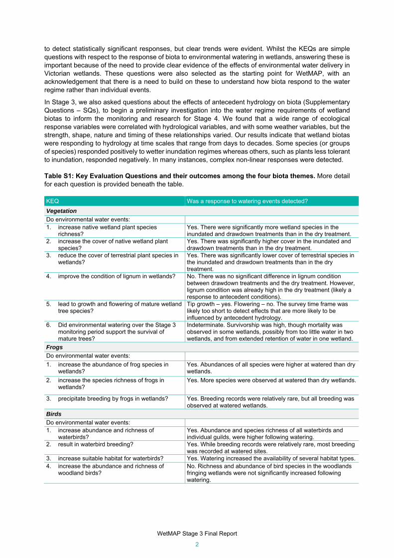
In Stage 3, all KEQs were evaluated. For most, there were significant, positive responses of the biota to environmental water events (see Table S1 below). In some cases, there was an insufficient sample size
WetMAP Stage 3 Final Report
2
to detect statistically significant responses, but clear trends were evident. Whilst the KEQs are simple questions with respect to the response of biota to environmental watering in wetlands, answering these is important because of the need to provide clear evidence of the effects of environmental water delivery in Victorian wetlands. These questions were also selected as the starting point for WetMAP, with an acknowledgement that there is a need to build on these to understand how biota respond to the water regime rather than individual events.
In Stage 3, we also asked questions about the effects of antecedent hydrology on biota (Supplementary Questions – SQs), to begin a preliminary investigation into the water regime requirements of wetland biotas to inform the monitoring and research for Stage 4. We found that a wide range of ecological response variables were correlated with hydrological variables, and with some weather variables, but the strength, shape, nature and timing of these relationships varied. Our results indicate that wetland biotas were responding to hydrology at time scales that range from days to decades. Some species (or groups of species) responded positively to wetter inundation regimes whereas others, such as plants less tolerant to inundation, responded negatively. In many instances, complex non-linear responses were detected.
Table S1: Key Evaluation Questions and their outcomes among the four biota themes. More detail for each question is provided beneath the table.
KEQ Was a response to watering events detected?
Vegetation
Do environmental water events: 1. increase native wetland plant species
richness? Yes. There were significantly more wetland species in the inundated and drawdown treatments than in the dry treatment.
2. increase the cover of native wetland plant species?
Yes. There was significantly higher cover in the inundated and drawdown treatments than in the dry treatment.
3. reduce the cover of terrestrial plant species in wetlands?
Yes. There was significantly lower cover of terrestrial species in the inundated and drawdown treatments than in the dry treatment.
4. improve the condition of lignum in wetlands? No. There was no significant difference in lignum condition between drawdown treatments and the dry treatment. However, lignum condition was already high in the dry treatment (likely a response to antecedent conditions).
5. lead to growth and flowering of mature wetland tree species?
Tip growth – yes. Flowering – no. The survey time frame was likely too short to detect effects that are more likely to be influenced by antecedent hydrology.
6. Did environmental watering over the Stage 3 monitoring period support the survival of mature trees?
Indeterminate. Survivorship was high, though mortality was observed in some wetlands, possibly from too little water in two wetlands, and from extended retention of water in one wetland.
Frogs
Do environmental water events:
1. increase the abundance of frog species in wetlands?
Yes. Abundances of all species were higher at watered than dry wetlands.
2. increase the species richness of frogs in wetlands?
Yes. More species were observed at watered than dry wetlands.
3. precipitate breeding by frogs in wetlands? Yes. Breeding records were relatively rare, but all breeding was observed at watered wetlands.
Birds
Do environmental water events: 1. increase abundance and richness of
waterbirds? Yes. Abundance and species richness of all waterbirds and individual guilds, were higher following watering.
2. result in waterbird breeding? Yes. While breeding records were relatively rare, most breeding was recorded at watered sites.
3. increase suitable habitat for waterbirds? Yes. Watering increased the availability of several habitat types. 4. increase the abundance and richness of
woodland birds? No. Richness and abundance of bird species in the woodlands fringing wetlands were not significantly increased following watering.

WetMAP Stage 3 Final Report
3
Vegetation
Do environmental water events increase native wetland species richness (KEQ 1) and cover (KEQ 2) and reduce the cover of terrestrial species (KEQ 3)?
Environmental water clearly increased both the richness and cover of native wetland species, and suppressed the cover of terrestrial species, which was very similar to the response resulting from natural inundation. This was demonstrated by significantly more wetland species and higher cover in the inundated and drawdown treatments than the dry treatment. Encouragingly, compared with native wetland species, very few introduced wetland species were recorded in most wetlands, and their cover was low. This is despite the prevalence of invasive introduced wetland species in irrigation channels that supply water to these wetlands. Annual terrestrial species, predominantly pasture grasses, were abundant, but these did not persist in most wetlands during the inundated and drawdown phases.
How does the antecedent water regime affect native wetland plant species richness (SQ 1) and cover (SQ 2)?
We found significant relationships between the richness and cover of aquatic species, such as Myriophyllum spp., Nardoo (Marsilea drummondii) and River Club-sedge (Schoenoplectus tabernaemontani), and the antecedent period of inundation. For mudflat species, such as Pale Knotweed (Persicaria lapathifolia), Common Sneezeweed (Centipeda cunninghamii) and Small Knotweed (Polygonum plebeium), we found an effect of prior inundation frequency on species richness and an effect of temperature on richness and cover. Substantially fewer species and lower cover were predicted when temperatures were higher during the three months prior to survey. This highlights the need to consider climate drivers such as El Nino that facilitate heatwaves when planning water delivery.
Do environmental water events improve the condition of lignum in wetlands (KEQ 4) and how does the antecedent water regime affect its condition (SQ 4)?
Environmental watering events did not increase the condition of lignum but notably, predicted and observed condition was relatively high (with low variance) in all treatments and wetlands, with only one exception (Neds Corner Central) – which had the driest antecedent inundation regime of all wetlands. Inundation period in the prior decade was the best predictor of condition, reaching a likely threshold near the upper end of the hydrological gradient (permanent inundation). However, we had very few data in the poor–moderate condition range and no sites that had experienced greater inundation. Including such data in future analyses will improve the likelihood of stronger predictions.
Do environmental water events lead to growth and flowering of mature wetland tree species (KEQ 5) and survivorship of mature trees (KEQ 6)?
We found a greater magnitude of tip growth in both River Red Gum and Black Box that had been inundated by environmental water, compared with those that had not been inundated (for >9 months). For Black
Fish
1. Is seasonal fish production (increase in the number of fish from late winter to summer) greater in wetlands that receive environmental water than in wetlands that do not?
Yes. Early findings support our conceptual model that greater inundation from environmental watering results in more fish.
2. Does watering regime influence native fish species richness and abundance in wetlands?
Perhaps. Greater native fish density was observed in naturally flooded wetlands and greater native species richness was observed in wetlands with long-term connections to the Murray River. However, these results were not statistically significant, and more data are required.
3. Do environmental water events provide opportunities for fish to move between wetlands and rivers?
Yes. There was directional movement of fish in wetland channels when environmental watering events provided connections with wetlands.
4. Do Murray Hardyhead (Craterocephalus fluviatilis) persist in saline wetlands where environmental water is effectively used to maintain wetland salinity levels within the range required for successful spawning and recruitment?
Yes. Relatively high abundances of Murray Hardyhead were only observed in wetlands and years when salinity was within the range required for successful spawning.

WetMAP Stage 3 Final Report
4
Box, this response was observed mainly in trees near the edge of one wetland (Little Lake Heywood), which had the largest population among the study wetlands. These trees were not subject to the deep, sustained inundation experienced in the middle of the wetland which resulted in high mortality there. Survival of mature River Red Gum was high among wetlands, despite 50% of the population not being inundated by environmental water. Some mortality did occur on elevated terraces which had not been inundated for ~10 years, suggesting that prolonged dry conditions have contributed to their mortality.
Frogs
Do environmental water events increase the abundance (KEQ1) and species richness (KEQ2) or precipitate breeding (KEQ3) of frogs in wetlands?
We identified a clear response to watering – frogs were significantly more abundant and exhibited greater species richness at watered sites (which would have been dry in the absence of watering) compared with dry ones. In general, watered sites had comparable abundances and numbers of frog species relative to sites that hold water permanently.
Little evidence of frog reproduction was recorded during surveys, although all records were from watered wetlands. The limited breeding response may be due to methodological limitations, or because watered wetlands do not maintain water for long enough to meet breeding requirements of some species.
What survey technique or combination of techniques is the most effective at detecting the greatest number of frog species and measuring abundance in wetlands (SQ1)?
Bioacoustic surveys are a promising method to monitor calling species like frogs, in terms of collecting data continuously over long timeframes (several weeks or months). Through a collaboration with the University of Melbourne, we have made considerable progress in developing and refining these methods. Bioacoustic surveys yielded recordings of species over longer time frames and returned recordings of the threatened Sloane’s froglet (Crinia sloanei), a species not recorded during audio-visual surveys. Combining bioacoustics surveys, using AudioMoth acoustic loggers, with audio-visual surveys resulted in a greater number of frog taxa per wetland than either technique would have delivered on its own. There are other challenges still to address to further refine bioacoustics methods in the future, especially honing the performance of call recognisers, and applying more sophisticated analytical methods (e.g. dynamic occupancy modelling) to more confidently assess the relationships between frog occupancy, variability in call detection, and responses to watering and other environmental predictors.
Preliminary exploration of frog relationships with hydrological regimes and habitat (Longer-term KEQs and SQs)
We found strong relationships for most frog species with hydrological predictors, typically the extent and duration of inundation. However, the importance of the antecedent watering period varied, generally related to the tadpole development times of different species. For instance, abundance of Crinia parinsignifera was best predicted by the proportion of wetlands that were wet in the preceding 30 days, while the abundance of Limnodynastes dumerilii was best predicted by the proportion of wetlands that was wet in the preceding 90 days. The response of different species to watering is likely to vary based on how long wetlands are inundated for, and there is a need to consider whether water remains long enough for tadpole development to be completed.
We also found that some habitat variables, especially tall emergent vegetation, influenced frog occurrence and abundance. This indicates that management of wetlands for frogs will likely need to consider both environmental watering and complementary management actions that support the maintenance or enhancement of vegetation.
Birds
Do environmental water events increase abundance and richness (KEQ1) and result in breeding (KEQ2) of waterbirds? Do environmental water events increase abundance and richness of woodland birds (KEQ4)?
Waterbirds responded quickly and strongly to environmental water, with increases in abundance and species richness. In contrast, although they occurred in vegetation that likely drew on groundwater provided by environmental water, terrestrial bird species in woodlands surrounding wetlands showed no

WetMAP Stage 3 Final Report
5
detectable short-term response to environmental water deliveries. These differences suggest waterbirds are more strongly impacted by watering.
After delivery of environmental water, we observed only a small number of birds, from a small number of species, breeding in and around wetlands. This may indicate that improvements to environmental water deliveries are needed to create suitable breeding habitat within watered wetlands, or it could reflect broader regional considerations. For example, breeding may be occurring elsewhere, or it could be that there is not enough water in the landscape to signal a breeding event in a particular wetland.
Do environmental water events increase suitable habitat for waterbirds (KEQ3)?
We found that several habitat types were used extensively by different waterbird species, especially deep open water and shallow open water, and bare wet substrate. Habitat associations often varied by different guilds and species. We found that environmental watering increased the availability of most habitats used by waterbirds. Some of these changes are obvious (i.e. watering leads to increased availability of deep and shallow open water). However, just because a wetland is watered does not guarantee all habitats will be present, but we did find increases in emergent plants, bare wet substrate, aquatic vegetation and bare dry substrate.
Preliminary examination of bird relationships with hydrological regimes and the importance of landscape water availability
The number of waterbirds was related to the duration of the antecedent period over which wetlands held water, and the different antecedent periods were important for different species. For example, numbers of Hoary-headed Grebe, Black-winged Stilts and Black Swans were strongly related to the proportion of wetlands that were wet on the day of sampling, in the past 30 days, and past 90 days, respectively. These inter-specific differences may relate to diet and foraging behaviour, with Hoary-headed Grebes foraging in deep water and largely on aquatic invertebrates that are likely to quickly colonise watered wetlands, whereas Black-winged Stilts forage on benthic infauna that may take longer to become established, and Black Swans feed on aquatic vegetation which takes an even more extended time to grow after delivery of environmental water. These results can help set expectations for when particular species are likely to respond to environmental watering.
We used a long time-series of bird counts from the Western Treatment Plant to demonstrate the local waterbird abundance and diversity was affected by continental rainfall patterns and water availability at locations in south-eastern Australia. Counts of several species were negatively correlated with water availability in the Goulburn-Loddon-Wimmera-Mallee catchments. Given the high mobility of many species, the availability of water elsewhere in the landscape is likely to be an important influence on local-scale responses, and in particular, responses to watering may be reduced in years when water availability is higher in other locations relative to in Victoria, with many birds moving elsewhere tracking surface water.
Fish
Is seasonal fish production (increase in the number of fish from late winter to summer) greater in wetlands that receive environmental water than in wetlands that do not (KEQ1)?
We found support for our hypothesis that greater area of inundation, using environmental water, results in more native fish being produced (through spawning, recruitment and survival). This was despite our control wetlands (those that did not receive water) drying completely, eliminating all native fishes and hampering our planned analysis. This question was intended to be answered over many years of ongoing sampling, but the first two years of sampling presented here provide insights into the relationships.
Does watering regime influence native fish species richness and abundance in wetlands (KEQ2)?
Following one year of investigation (COVID19 hampered sampling for this question in 2020), we have observed results that support our hypotheses relating to the impacts of water regime (over several years) on wetland fish populations. First, we observed greater native fish density in wetlands with a natural watering regime (multiple late winter/spring inundation events) than in those with stable water levels or annual watering events. Second, we observed greater native species richness in wetlands with stable water levels (with long-term connections to the Murray River) than in the other two classifications. However, these results were not statistically significant, and more data are required to answer this

WetMAP Stage 3 Final Report
6
question. Future incorporation of fish data collected for The Living Murray Program may increase our statistical power to demonstrate the impacts of water regime on fishes.
Do environmental water events provide opportunities for fish to move between wetlands and rivers (KEQ3)?
We have demonstrated that there is directional movement of fish in wetland channels when environmental watering events provide connections with wetlands. In addition, we have demonstrated that adult Australian Smelt (Retropinna semoni) immigrate into wetlands (prior to their spawning period) when environmental water is flowing into wetlands and providing connectivity for fish. This connectivity also resulted in the dispersal of juvenile Australian Smelt and Carp Gudgeon (Hypseleotris spp.) out of wetlands following spawning. This demonstrates the potential for environmental water to enable large-scale emigration of fish (we observed over 1800 per wetland per day) and nutrients from wetlands to rivers if sufficient hydrological connectivity is provided.
Do Murray Hardyhead (Craterocephalus fluviatilis) persist in saline wetlands where environmental water is effectively used to maintain wetland salinity levels within the range required for successful spawning and recruitment (KEQ4)?
We observed relatively high abundances of Murray Hardyhead, but only in wetlands and years when salinity was within the range required for successful spawning. In two highly saline wetlands, environmental water was successfully used to decrease salinity concentrations during the species’ spawning period, below the threshold recommended for the survival of eggs and larvae. Salinity concentrations then increased later in the year, likely reducing the abundance of competitors (particularly Eastern Gambusia (Gambusia holbrooki)) and reducing negative interactions between species, such as competition for food and interspecific aggression. Murray Hardyhead abundance was high in these wetlands. In brackish wetlands (lower salinity concentrations, but not freshwater), we observed high abundance of Murray Hardyhead in a wetland with dense aquatic vegetation and very low numbers in a wetland with lower aquatic vegetation densities. Density of aquatic vegetation may impact the persistence of Murray Hardyhead in some Victorian wetlands.

WetMAP Stage 3 Final Report
7
1 Introduction
This report details outcomes from vegetation, frog, bird and fish monitoring conducted for Stage 3 of the Wetland Monitoring and Assessment Program for environmental water (WetMAP).
In this first chapter, we provide an overview of WetMAP’s earlier stages, and the planning, governance, collaboration and information management relevant to Stage 3. This is followed by background, methods, results and discussion (including implications for management) for each biota theme (Chapters 2–5), and an overview of communications and engagement, including WetMAP’s citizen science projects (Chapter 6). We conclude with a summary of key findings and suggested next steps for Stage 4 (Chapter 7).
Each chapter is presented with relevant references, so they can be read as standalone documents. Extensive appendices are provided at the end of the report. These provide some of the more technical detail and contextual information to support the results and recommendations.
WetMAP Stages 1 and 2 The acquisition and delivery of water for the environment by the Victorian and Commonwealth governments represents a significant investment in aquatic ecosystem health and rehabilitation. Victoria currently holds 1,229,327 ML of water for the environment (‘environmental water’). Many agencies work together to develop and implement management plans to deliver this water, including the Department of Environment, Land, Water and Planning (DELWP), the Victorian Environmental Water Holder (VEWH), Catchment Management Authorities (CMAs), Melbourne Water, land managers, water authorities, the Commonwealth Environmental Water Office (CEWO) and the Murray–Darling Basin Authority (MDBA).
Maximising the efficiency and effectiveness of environmental water requires clear ecological objectives and an adaptive management framework that builds on evidence and key learnings from environmental watering outcomes.
With this in mind, WetMAP was established to investigate the responses of wetland biota to environmental water management in Victorian wetlands and to provide new information to support adaptive flow-management decisions. WetMAP is the companion program to the Victorian Environmental Flows Monitoring and Assessment Program (VEFMAP), which was initiated in 2004 to investigate outcomes from environmental flows in rivers.
WetMAP was established in 2014 (Stage 1, 2014–2015) and involved the development of a program framework, and identification of key knowledge gaps and priority questions for investigation (Jacobs 2015a, b, c). This process involved considerable consultation with Victorian CMAs and a range of technical experts.
Stage 2 (2015–2016) was coordinated by Water’s Edge Consulting and included an intensive consultation process between DELWP, the Water’s Edge Consulting team, Victorian CMAs, the VEWH, and discipline experts from various organisations, including the Arthur Rylah Institute (ARI), DELWP. The main outcome from Stage 2 was a set of program manuals: Part A – Program Reference (DELWP 2016a) and Part B – Field Monitoring Reference (DELWP 2016b). These manuals outline the program context, objectives and design options, including the statistical rationale behind the selection of ‘treatment’ and ‘control’ wetlands, high-level Key Evaluation Questions (KEQs) for each of the recommended key evaluation themes (native fish, vegetation, waterbirds and frogs), and a proposed approach to program monitoring, evaluation and reporting.
Upon completion, the manuals were reviewed by members of a scientific Independent Review Panel (IRP), who provided extensive constructive feedback and recommendations that formed the basis of the initial planning and development phases for Stage 3 (Section 1.5).
WetMAP in the Victorian monitoring and reporting context WetMAP is consistent with the adaptive management framework identified in the Victorian Waterway Management Strategy (DEPI 2013, Figure 1.1). Stage 3 was designed with the understanding that aspects of the program, including survey design, may change, depending on progress, advice, recommendations and the outcomes of sampling. Ongoing evaluation and performance monitoring of all aspects of the program, including governance, communication and engagement, and monitoring and research, have

WetMAP Stage 3 Final Report
8
ensured a flexible and responsive approach, which has enabled continuous improvement throughout Stage 3 (2017–2020).
Figure 1.1: The adaptive management cycle underpinning the Victorian Waterway Management Strategy (DEPI 2013). WetMAP is one of a set of monitoring programs overseen by the DELWP Catchment, Waterways, Cities and Towns (CWCT) division. Riparian and Wetland Intervention Monitoring Programs (RIMP and WIMP) are currently being implemented. These long-term programs aim to evaluate the effectiveness of riparian and wetland management (other than using environmental flows) and will demonstrate responses to a range of different management approaches over time. As mentioned, DELWP also manages VEFMAP, which examines ecological outcomes from environmental flows in rivers across Victoria, using a combination of targeted research, long-term condition monitoring and event-based intervention monitoring.
Program governance WetMAP Stage 3 was delivered through a close collaboration between DELWP’s CWCT division and ARI. The program operated using a centralised governance model (Figure 1.2) and was funded through the Victorian Government’s $222 million investment to improve the health of waterways and catchments under Water for Victoria.
The WetMAP project team included two program management staff from CWCT, as well as ARI scientists and communication personnel. Members of the IRP, Project Steering Committee (PSC) and CMA environmental water managers were also integral to the delivery of the program.

WetMAP Stage 3 Final Report
9
Figure 1.2: WetMAP Stage 3 governance model.
Program objectives and themes There were three overarching objectives for WetMAP Stage 3:
1. to enable DELWP and its water delivery partners to clearly demonstrate the ecological value of environmental water management to the community and water industry stakeholders
2. to fill knowledge gaps to improve planning, delivery and evaluation of environmental water management in wetlands across Victoria
3. to identify ecosystem outcomes from environmental water to help meet Victoria’s obligations under the Murray–Darling Basin Plan (Schedule 12, Matter 8).
These are consistent with the objectives of VEFMAP Stage 6.
Program monitoring themes included vegetation, frogs, waterbirds (and woodland birds), and fish. These key themes were recommended in Stage 1 and reflect the knowledge gaps and needs of CMA wetland managers for informing environmental water management actions and demonstrating outcomes to the community.
Stage 3 planning, monitoring questions and evaluation
Planning and commencement of monitoring WetMAP underwent a phase of planning, method evaluation and implementation throughout 2017, based on IRP input during Stage 2 (Table 1.1).
Specific activities included:
statistical design workshops for the vegetation, bird, fish and frog themes
an investigation into the availability and selection of ‘control’ and/or counterfactual wetlands
a pilot project in autumn 2017 to evaluate the efficacy of vegetation survey methods and collect data enabling power analyses to confirm sample sizes for KEQ evaluation

WetMAP Stage 3 Final Report
10
a review of the KEQs proposed in the program manuals, following detailed discussions with Victorian CMAs
selection of wetlands for monitoring
a literature review
a review of objectives, conceptual models and knowledge gaps for native fish
an exploration of alternative methods for data collection for frogs.
Monitoring commenced in 2017–2018 for vegetation, followed by birds, fish and frogs in 2018–2019 (Table 1.1).
Table 1.1: Timing of commencement of monitoring for each evaluation theme.
Theme Year
Jan–June 2017 2017–2018 2018–2019 2019–2020
Vegetation Planning
Pilot methods Year 1 data Year 2 data
Year 3 data Analysis and reporting
Birds Planning Pilot methods and
design Year 1 data
Year 2 data Analysis and reporting
Fish Planning Pilot methods and
design Year 1 data
Year 2 data Analysis and reporting
Frogs – Planning Year 1 data Year 2 data
Analysis and reporting
Revision of Key Evaluation Questions and development of Supplementary Questions
The revision of the KEQs developed in Stage 3 was iterative, reflecting our adaptive approach to the program. Initial KEQs developed in Stage 2 were informed by objectives in CMA Environmental Water Management Plans (EWMPs), Murray–Darling Basin Plan (MDBP) Long Term Watering Plans (LTWPs) and the VEWH’s Seasonal Watering Plans (DELWP 2016a). In the first year of Stage 3, questions were adjusted following a series of workshops, individual meetings with CMAs and independent expert advice from IRP members. In early 2019–2020, based on the results of monitoring data, KEQs and conceptual models underpinning the program underwent further review, and a set of SQs and revised KEQs were developed for each theme. These questions are:
realistically answerable and able to demonstrate the value of environmental water to regional, state-wide and Commonwealth stakeholders and the community
based on the latest conceptual understanding of ecological responses to flow
directly relevant to key knowledge gaps for environmental water management
able to complement rather than duplicate data collections under way for other monitoring programs.
KEQs and SQs were outlined in the 2019–2020 monitoring plans for each theme, which were distributed to CMAs and other stakeholders.
The KEQs developed for WetMAP Stage 3 enabled the program to deliver on two objectives during the time frame available for monitoring (up to 3 years): Objective 1 (to demonstrate the ecological value of environmental water in wetlands), and Objective 3 (report on Basin Plan outcomes for BP 5-yearly Schedule 12, Matter 8 reporting).
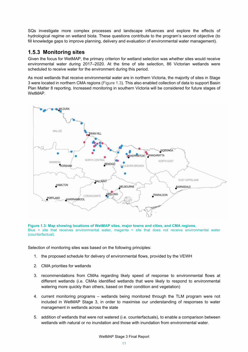
WetMAP Stage 3 Final Report
11
SQs investigate more complex processes and landscape influences and explore the effects of hydrological regime on wetland biota. These questions contribute to the program’s second objective (to fill knowledge gaps to improve planning, delivery and evaluation of environmental water management).
Monitoring sites Given the focus for WetMAP, the primary criterion for wetland selection was whether sites would receive environmental water during 2017–2020. At the time of site selection, 86 Victorian wetlands were scheduled to receive water for the environment during this period.
As most wetlands that receive environmental water are in northern Victoria, the majority of sites in Stage 3 were located in northern CMA regions (Figure 1.3). This also enabled collection of data to support Basin Plan Matter 8 reporting. Increased monitoring in southern Victoria will be considered for future stages of WetMAP.
Figure 1.3: Map showing locations of WetMAP sites, major towns and cities, and CMA regions. Blue = site that receives environmental water, magenta = site that does not receive environmental water (counterfactual). Selection of monitoring sites was based on the following principles:
1. the proposed schedule for delivery of environmental flows, provided by the VEWH
2. CMA priorities for wetlands
3. recommendations from CMAs regarding likely speed of response to environmental flows at different wetlands (i.e. CMAs identified wetlands that were likely to respond to environmental watering more quickly than others, based on their condition and vegetation)
4. current monitoring programs – wetlands being monitored through the TLM program were not included in WetMAP Stage 3, in order to maximise our understanding of responses to water management in wetlands across the state
5. addition of wetlands that were not watered (i.e. counterfactuals), to enable a comparison between wetlands with natural or no inundation and those with inundation from environmental water.

WetMAP Stage 3 Final Report
12
Control sites and counterfactuals Assessments of the effects of environmental flows are often hampered by a lack of control sites for comparison (Cottingham et al. 2005; Webb et al. 2010). As Victoria’s wetlands are naturally highly variable, locating suitable ‘control’ sites is a challenge. True control sites for this program should ideally be as similar as possible to the sites that receive environment water, without receiving environmental flows themselves (Cottingham et al. 2005). Ideally, this would require selection of sites that have experienced the same hydrological regime, have a similar landscape setting and have other characteristics similar to the environmental water sites.
Finding perfectly paired sites of this description was not possible. Given this, the approach taken for WetMAP Stage 3 was to identify ‘control sites’ that were as similar as possible to the watered wetlands selected for monitoring. In recognition of the fact that these are not true ‘controls’ in terms of experimental protocol, the term ‘counterfactual sites’ was adopted. In this sense, the counterfactual wetland is the best attempt to select a site that represents the condition the watered site would show if it did not receive environmental flows. Analyses have included a comparison of ecological responses in the treatment and counterfactual sites.
Selecting ‘counterfactual’ sites for WetMAP Stage 3 involved two approaches:
1. a desk-top analysis comparing individual treatment wetlands with a complete list of non-watered wetlands across the state
2. recommendations from CMAs and experienced field scientists of sites with similar watering histories and flora and fauna communities.
The counterfactual sites selected for each theme reflect the different KEQs and statistical design needs for that theme. Further details are provided in each theme chapter.
Informing adaptive management and CMA water management plans Annual monitoring plans were reviewed by the IRP prior to distribution to CMAs and other interested stakeholders. All modifications and refinements made to the study design, including changes to sites, methods, KEQs, and the introduction of SQs, were included in these plans as a means of informing CMAs about the program approach for the coming year.
Data collected in Stage 3 have been analysed and reported annually, with results provided to CMA waterway managers soon after monitoring completion, to guide timely discussions and decisions regarding environmental water delivery.
Regular communication between the WetMAP project team and CMAs, the VEWH and other relevant stakeholders allowed direct input of information and learnings into decision-making processes for environmental water deliveries. Results from monitoring have informed changes to the timing of watering events and enabled delivery of desired hydrographs to support waterbird foraging. Information gained through WetMAP has also informed the development of annual seasonal watering proposals (and subsequent Seasonal Watering Plans; e.g. VEWH 2020). Further information on this is presented in Chapter 7 “Communication and Engagement”.
Collaborations Results from WetMAP Stage 3 have been significantly improved by close collaboration and sharing of knowledge, data and learnings with a broad range of scientists, research institutes and agencies (Table 1.2). WetMAP is one of several environmental water monitoring programs in south-eastern Australia – others include the CEWO’s Monitoring, Evaluation and Research program (Flow-MER; previously LTIM and EWKR), TLM, VEFMAP and Melbourne Water’s river and wetland monitoring programs.
Partnerships with these and other programs and organisations have enabled effective sharing of knowledge, data and results and a more efficient use of funds, by sharing effort, expertise and equipment.
A collaboration with the Geoscience Australia (GA) Digital Earth Australia Product Development team facilitated access to the GA Wetland Insights Tool (WIT) product (Dunn et al. 2019). The tool is based on algorithms that detect water from Landsat data (see Appendix 3). Data from the tool were used to describe the effects of the antecedent water regime on biota for each of the WetMAP themes.
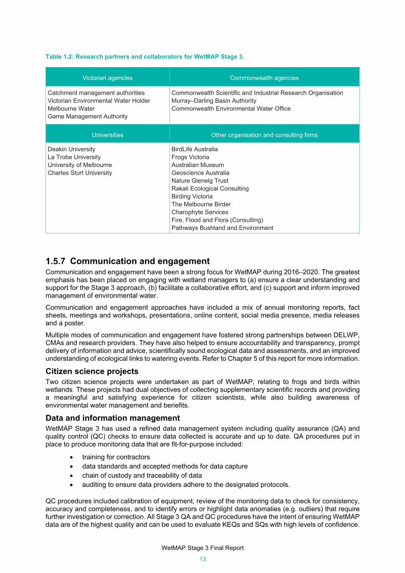
WetMAP Stage 3 Final Report
13
Table 1.2: Research partners and collaborators for WetMAP Stage 3.
Victorian agencies Commonwealth agencies
Catchment management authorities Victorian Environmental Water Holder Melbourne Water Game Management Authority
Commonwealth Scientific and Industrial Research Organisation Murray–Darling Basin Authority Commonwealth Environmental Water Office
Universities Other organisation and consulting firms
Deakin University La Trobe University University of Melbourne Charles Sturt University
BirdLife Australia Frogs Victoria Australian Museum Geoscience Australia Nature Glenelg Trust Rakali Ecological Consulting Birding Victoria The Melbourne Birder Charophyte Services Fire, Flood and Flora (Consulting) Pathways Bushland and Environment
Communication and engagement Communication and engagement have been a strong focus for WetMAP during 2016–2020. The greatest emphasis has been placed on engaging with wetland managers to (a) ensure a clear understanding and support for the Stage 3 approach, (b) facilitate a collaborative effort, and (c) support and inform improved management of environmental water.
Communication and engagement approaches have included a mix of annual monitoring reports, fact sheets, meetings and workshops, presentations, online content, social media presence, media releases and a poster.
Multiple modes of communication and engagement have fostered strong partnerships between DELWP, CMAs and research providers. They have also helped to ensure accountability and transparency, prompt delivery of information and advice, scientifically sound ecological data and assessments, and an improved understanding of ecological links to watering events. Refer to Chapter 5 of this report for more information.
Citizen science projects Two citizen science projects were undertaken as part of WetMAP, relating to frogs and birds within wetlands. These projects had dual objectives of collecting supplementary scientific records and providing a meaningful and satisfying experience for citizen scientists, while also building awareness of environmental water management and benefits.
Data and information management WetMAP Stage 3 has used a refined data management system including quality assurance (QA) and quality control (QC) checks to ensure data collected is accurate and up to date. QA procedures put in place to produce monitoring data that are fit-for-purpose included:
training for contractors data standards and accepted methods for data capture chain of custody and traceability of data auditing to ensure data providers adhere to the designated protocols.
QC procedures included calibration of equipment, review of the monitoring data to check for consistency, accuracy and completeness, and to identify errors or highlight data anomalies (e.g. outliers) that require further investigation or correction. All Stage 3 QA and QC procedures have the intent of ensuring WetMAP data are of the highest quality and can be used to evaluate KEQs and SQs with high levels of confidence.
WetMAP Stage 3 Final Report
14
WetMAP data are stored in a Microsoft SQL Server relational database. The database has in-built QA measures to ensure consistency in the data entered. A user-friendly database interface allows CMA staff to view and extract data summaries relevant to their area; external users are not able to input or change data. Data can be extracted by the curator, in consultation with data users. The curator works closely with the research team to develop data queries that meet ongoing reporting needs. During the reporting phase, if any anomalies in the data are detected they can be investigated and rectified where appropriate.
References Cottingham P., Quinn G., Norris R., King A., Chessman B. and Marshall C. (2005). Environmental flows
monitoring and assessment framework. Technical report. CRC for Freshwater Ecology, Canberra, ACT.
DELWP. (2016a). WetMAP Manual: Part A Program Reference. Department of Environment, Land, Water and Planning, Victoria.
DELWP. (2016b). WetMAP Manual: Part B Field Monitoring Reference. Department of Environment, Land, Water and Planning, Victoria.
Dunn, B., Lymburner, L., Newey, V., Hicks, A. and Carey, H. (2019). Developing a Tool for Wetland Characterization Using Fractional Cover, Tasseled Cap Wetness and Water Observations from Space, IGARSS 2019–2019 IEEE International Geoscience and Remote Sensing Symposium, Yokohama, Japan, 2019, pp. 6095–6097, doi: 10.1109/IGARSS.2019.8897806.
Jacobs (2015a). WetMAP Stage 1 report: literature review. Jacobs Group (Australia), report prepared for the Department of Environment, Land, Water and Planning, Melbourne, Victoria.
Jacobs (2015b). WetMAP Stage 1 report: summary of questions posed by water managers and technical specialists. Jacobs Group (Australia), report prepared for the Department of Environment, Land, Water and Planning, Melbourne, Victoria.
Jacobs (2015c). WetMAP Stage 1 report: potential monitoring questions that WetMAP can address. Jacobs Group (Australia), report prepared for the Department of Environment, Land, Water and Planning, Melbourne, Victoria.
VEWH. (2020). 2020–21 Seasonal Watering Plan. Victorian Environmental Water Holder, Melbourne, Victoria. https://www.vewh.vic.gov.au/watering-program/seasonal-watering-plan
Webb, J.A., Stewardson, M.J. and Koster, W.M. (2010). Detecting ecological responses to flow variation using Bayesian hierarchical models. Freshwater Biology, 55: 108–126.

WetMAP Stage 3 Final Report
15
2 Vegetation theme
Introduction
Wetland vegetation in Victoria Victoria’s wetland vegetation is diverse and plays an essential role in the function and structure of its wetland ecosystems. The composition, structure and diversity of wetland vegetation varies within and between wetlands, ranging from herbaceous treeless communities such as aquatic grassy wetlands and herblands, to woodlands and forests dominated by trees such as River Red Gum (Eucalyptus camaldulensis subsp. camaldulensis) and Black Box (Eucalyptus largiflorens) (DSE 2012). This diversity is reflected in the 151 Ecological Vegetation Classes (EVCs) that have been described for wetlands in Victoria, defined by species composition and structure (DELWP 2018). Variation in wetland vegetation, even within EVCs, is driven by environmental variation (e.g. in inundation patterns, rainfall, soil type and land-use practices surrounding the wetlands) at multiple spatial and temporal scales. An individual wetland can support a sequence of plant communities, from the deepest part of the wetland, which retains water for the longest period, to the peripheral verges, which are subject to only intermittent and temporary inundation events (Brock and Casanova 1997; Capon 2005). Variability in wetland vegetation is expressed both along ecological gradients within an individual wetland (most notably elevational or hydrological gradients) and between comparable zones of other wetlands.
Victoria’s wetland vegetation provides many important functions. These include the provision of habitat and food resources for other biota such as birds, frogs and fish, erosion reduction through sediment stabilisation, primary productivity and nutrient cycling, interconnecting links between aquatic and terrestrial ecosystems, dispersal corridors for biota across the landscape, and aesthetic value for people (DSE 2005; Roberts and Marston 2011; Morris 2012; Dobbie 2013).
Responses of wetland vegetation to inundation The response of wetland vegetation to a single inundation event is dependent on the hydrological characteristics of the event itself and the local weather conditions, as well as on the historic and antecedent factors that have influenced the condition of the vegetation community prior to the event (Casanova and Brock 2000; Roberts et al. 2017) (Figure 2.1). Developing an understanding of the impacts of the historic and antecedent events on wetland vegetation condition provides essential context for evaluating the response of a wetland vegetation community, or a particular species, to a particular inundation cycle, such as an individual environmental watering event (Figure 2.1). In Victoria, regional management plans provide some historic data regarding water management and resultant impacts on wetland water regimes dating back to the 1950s, and satellite data provide valuable high-frequency wetland inundation extent data from 1987.

WetMAP Stage 3 Final Report
16
Figure 2.1: Conceptual model illustrating the influence of antecedent factors and water regime characteristics on wetland condition, in turn affecting vegetation responses to an inundation event. An inundation event results in a sequenced vegetation response over the course of the event cycle (inundation, drawdown, drying and dry phases). Hydrological components of the inundation event are relevant to the responses of different types of wetland species. Biotic processes such as competition, herbivory and dispersal also affect the vegetation condition at the time of the first inundation event and vegetation responses to the inundation event. The vegetation condition following drawdown and recent drying after the inundation event therefore reflects the outcome of the event as well as the historic and antecedent factors that preceded it.
Vegetation responses to a single inundation event cycle In temporary wetlands, a single inundation event results in a sequenced vegetation response as the wetland fills, draws down and then becomes dry (Figure 2.1, Figure 2.2). The response of the various wetland species to the event depends on their ability to germinate, establish, grow, reproduce and disperse in response to the changing hydrological conditions, and the characteristics of the propagule bank present (Brock and Casanova 1997; Casanova and Brock 2000; Casanova 2011; Roberts et al. 2017). The abundance of wetland plants begins to increase as water levels draw down, peaks after waters have receded but soil moisture is still high, and then decreases as soil moisture declines (Figure 2.2) (Campbell et al. 2019a). This means that peaks in the total wetland plant species abundance can occur well after drawdown; for example, at Hattah Lakes in north-western Victoria, native wetland plant abundance peaked at 50–60 days after the last inundation event, while the abundance of species preferring drier conditions peaked at 90–200 days (James et al. 2019). As such, the timing of monitoring surveys in relation to the inundation event is an important consideration in understanding the observed responses of the wetland vegetation present (Figure 2.2).
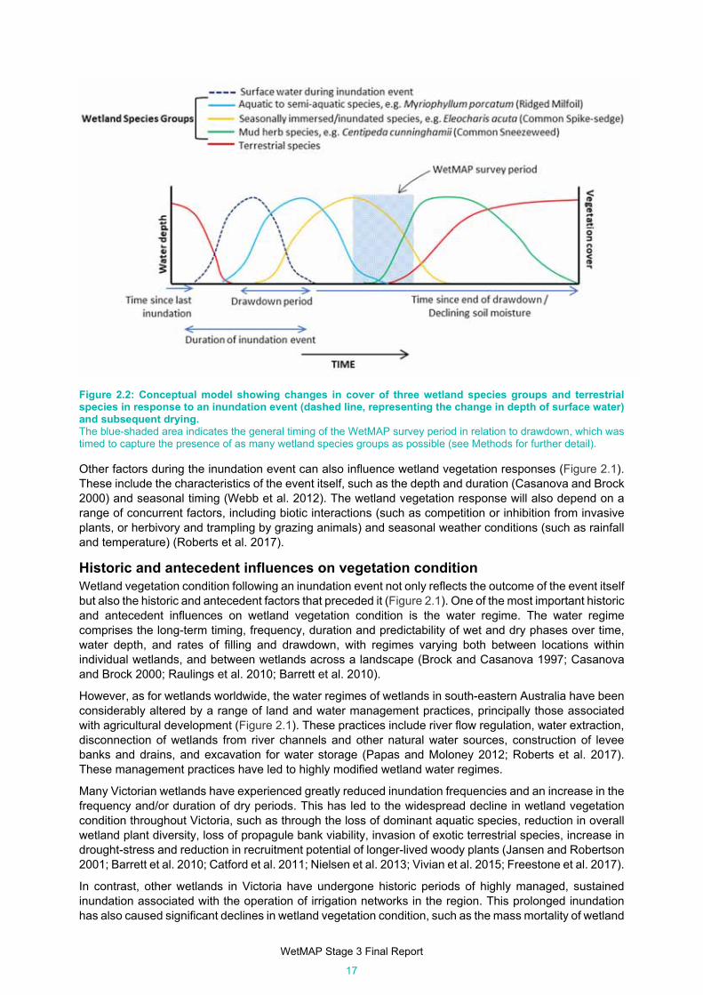
WetMAP Stage 3 Final Report
17
Figure 2.2: Conceptual model showing changes in cover of three wetland species groups and terrestrial species in response to an inundation event (dashed line, representing the change in depth of surface water) and subsequent drying. The blue-shaded area indicates the general timing of the WetMAP survey period in relation to drawdown, which was timed to capture the presence of as many wetland species groups as possible (see Methods for further detail). Other factors during the inundation event can also influence wetland vegetation responses (Figure 2.1). These include the characteristics of the event itself, such as the depth and duration (Casanova and Brock 2000) and seasonal timing (Webb et al. 2012). The wetland vegetation response will also depend on a range of concurrent factors, including biotic interactions (such as competition or inhibition from invasive plants, or herbivory and trampling by grazing animals) and seasonal weather conditions (such as rainfall and temperature) (Roberts et al. 2017).
Historic and antecedent influences on vegetation condition Wetland vegetation condition following an inundation event not only reflects the outcome of the event itself but also the historic and antecedent factors that preceded it (Figure 2.1). One of the most important historic and antecedent influences on wetland vegetation condition is the water regime. The water regime comprises the long-term timing, frequency, duration and predictability of wet and dry phases over time, water depth, and rates of filling and drawdown, with regimes varying both between locations within individual wetlands, and between wetlands across a landscape (Brock and Casanova 1997; Casanova and Brock 2000; Raulings et al. 2010; Barrett et al. 2010).
However, as for wetlands worldwide, the water regimes of wetlands in south-eastern Australia have been considerably altered by a range of land and water management practices, principally those associated with agricultural development (Figure 2.1). These practices include river flow regulation, water extraction, disconnection of wetlands from river channels and other natural water sources, construction of levee banks and drains, and excavation for water storage (Papas and Moloney 2012; Roberts et al. 2017). These management practices have led to highly modified wetland water regimes.
Many Victorian wetlands have experienced greatly reduced inundation frequencies and an increase in the frequency and/or duration of dry periods. This has led to the widespread decline in wetland vegetation condition throughout Victoria, such as through the loss of dominant aquatic species, reduction in overall wetland plant diversity, loss of propagule bank viability, invasion of exotic terrestrial species, increase in drought-stress and reduction in recruitment potential of longer-lived woody plants (Jansen and Robertson 2001; Barrett et al. 2010; Catford et al. 2011; Nielsen et al. 2013; Vivian et al. 2015; Freestone et al. 2017).
In contrast, other wetlands in Victoria have undergone historic periods of highly managed, sustained inundation associated with the operation of irrigation networks in the region. This prolonged inundation has also caused significant declines in wetland vegetation condition, such as the mass mortality of wetland
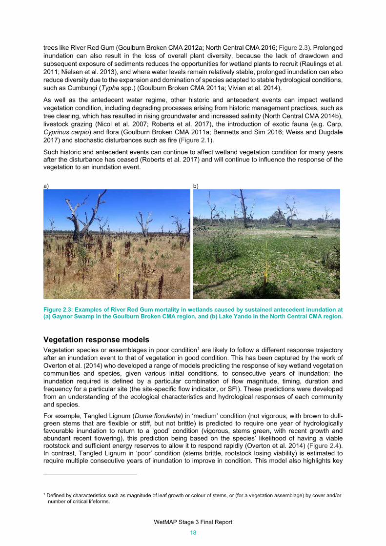
WetMAP Stage 3 Final Report
18
trees like River Red Gum (Goulburn Broken CMA 2012a; North Central CMA 2016; Figure 2.3). Prolonged inundation can also result in the loss of overall plant diversity, because the lack of drawdown and subsequent exposure of sediments reduces the opportunities for wetland plants to recruit (Raulings et al. 2011; Nielsen et al. 2013), and where water levels remain relatively stable, prolonged inundation can also reduce diversity due to the expansion and domination of species adapted to stable hydrological conditions, such as Cumbungi (Typha spp.) (Goulburn Broken CMA 2011a; Vivian et al. 2014).
As well as the antedecent water regime, other historic and antecedent events can impact wetland vegetation condition, including degrading processes arising from historic management practices, such as tree clearing, which has resulted in rising groundwater and increased salinity (North Central CMA 2014b), livestock grazing (Nicol et al. 2007; Roberts et al. 2017), the introduction of exotic fauna (e.g. Carp, Cyprinus carpio) and flora (Goulburn Broken CMA 2011a; Bennetts and Sim 2016; Weiss and Dugdale 2017) and stochastic disturbances such as fire (Figure 2.1).
Such historic and antecedent events can continue to affect wetland vegetation condition for many years after the disturbance has ceased (Roberts et al. 2017) and will continue to influence the response of the vegetation to an inundation event.
a) b)
Figure 2.3: Examples of River Red Gum mortality in wetlands caused by sustained antecedent inundation at (a) Gaynor Swamp in the Goulburn Broken CMA region, and (b) Lake Yando in the North Central CMA region.
Vegetation response models Vegetation species or assemblages in poor condition1 are likely to follow a different response trajectory after an inundation event to that of vegetation in good condition. This has been captured by the work of Overton et al. (2014) who developed a range of models predicting the response of key wetland vegetation communities and species, given various initial conditions, to consecutive years of inundation; the inundation required is defined by a particular combination of flow magnitude, timing, duration and frequency for a particular site (the site-specific flow indicator, or SFI). These predictions were developed from an understanding of the ecological characteristics and hydrological responses of each community and species.
For example, Tangled Lignum (Duma florulenta) in ‘medium’ condition (not vigorous, with brown to dull-green stems that are flexible or stiff, but not brittle) is predicted to require one year of hydrologically favourable inundation to return to a ‘good’ condition (vigorous, stems green, with recent growth and abundant recent flowering), this prediction being based on the species’ likelihood of having a viable rootstock and sufficient energy reserves to allow it to respond rapidly (Overton et al. 2014) (Figure 2.4). In contrast, Tangled Lignum in ‘poor’ condition (stems brittle, rootstock losing viability) is estimated to require multiple consecutive years of inundation to improve in condition. This model also highlights key
1 Defined by characteristics such as magnitude of leaf growth or colour of stems, or (for a vegetation assemblage) by cover and/or
number of critical lifeforms.

WetMAP Stage 3 Final Report
19
knowledge gaps, with the maximum dry period duration that Tangled Lignum can tolerate while still remaining viable and responsive to the next inundation event not yet quantified (Overton et al. 2014; Freestone et al. 2017).
Figure 2.4: Predicted improvement in the condition of lignum with different initial levels of condition (good, medium, poor or critical) following consecutive years of the site-specific flow indicator (SFI) being met; described as ‘preference curves’ by Overton et al. (2014; p. 63). The SFI is a specific combination of flow magnitude, timing, duration and frequency at a particular site (see Overton et al. 2014 for further details).
WetMAP vegetation monitoring questions: development and rationale Key Evaluation Questions (KEQs) and Supplementary Questions (SQs) for vegetation (Table 2.1) were developed to address WetMAP objectives (see Chapter 1). The focus of the KEQs was on assessing responses to watering events, including both natural and managed. However, we also investigated (through SQs) the effects of the antecedent water regime on vegetation, to inform a more in-depth assessment in Stage 4 of WetMAP (identification of water regime requirements and thresholds). SQ 3 and SQ 5 could not be addressed in Stage 3 due to time constraints and SQ 6 and SQ 7 involve effects with longer response times and require further data collection over subsequent years. Therefore, although data were collected for these questions during Stage 3, the results are not presented here but will be addressed in a later stage.
The KEQs and SQs incorporate measures commonly included as objectives in Victorian CMA Environmental Water Management Plans (EWMPs), including wetland species richness and cover, the recruitment of woody species, cover of terrestrial species, and measures related specifically to ecologically significant and widespread wetland plant species such as Tangled Lignum, River Red Gum and Black Box, as well as specific wetland vegetation communities, such as Tall Marsh, which is an emergent macrophyte community usually dominated by Cumbungi or Common Reed (Phragmites australis).

WetMAP Stage 3 Final Report
20
Table 2.1: WetMAP vegetation Key Evaluation Questions (KEQs) and Supplementary Questions (SQs). Shaded questions were evaluated in this stage of WetMAP. Unshaded questions were not able to be addressed in this stage of WetMAP.
Key Evaluation Question Related Supplementary Question
1. Do environmental water events increase native wetland plant species richness?
1. How does the antecedent water regime affect native wetland plant species richness?
2. Do environmental water events increase the cover of native wetland plant species?
2. How does the antecedent water regime affect the cover of native wetland plant species?
3. Do environmental water events reduce the cover of terrestrial plant species in wetlands?
3. How does the antecedent water regime affect the cover of terrestrial plant species in wetlands?
4. Do environmental water events improve the condition of lignum in wetlands?
4. How does the antecedent water regime affect the condition of lignum in wetlands?
5. Do environmental water events lead to growth and flowering of mature wetland tree species?
5. How does the antecedent water regime affect the tip growth and flowering of mature wetland tree species?
6. Did environmental water support survival of mature trees?
6. How does the antecedent water regime affect the recruitment of juveniles and saplings?
7. How does the antecedent water regime affect the extent of the native colonists Typha and Phragmites in wetlands?
Lignum is considered to be the most significant wetland shrub across the Murray–Darling Basin. Lignum occurs in wetlands across the western and northern parts of Victoria and can form extensive shrublands as well as occur in the understorey of woodlands (Roberts and Marston 2011). Lignum provides important habitat during both dry and flooded conditions for a range of fauna such as waterbirds, aquatic invertebrates, fish and terrestrial animals (Frood 2007a; Roberts and Marston 2011; Figure 2.5). Lignum, however, can replace herbaceous vegetation in some areas, including formerly open wetlands, where it can colonise and form dense stands (Frood 2007a, 2007b).
River Red Gum is widely distributed across Victoria and is the dominant and often the only tree species in frequently flooded floodplain and wetland forests and woodlands. Black Box occurs in north-western Victoria, where it is often the dominant woodland tree species at higher and thus less frequently flooded elevations, compared with River Red Gum. Given their dominance and widespread distribution, both tree species are critically important to the ecology of rivers and wetlands, providing habitat and food resources for an enormous range of aquatic and terrestrial fauna (Roberts and Marston 2011). Tall Marsh is also an important wetland vegetation community, particularly because of its provision of habitat for waterbirds and frogs; however, in some wetlands in Victoria, because of prolonged or frequent inundation, it has increased in extent, and caused a reduction in diversity of habitats. The control of this plant community is often a key management objective (North Central CMA 2015a; GHD 2017).

WetMAP Stage 3 Final Report
21
a) b)
Figure 2.5: Lignum provides habitat for cryptic bird species and nesting birds. (a) Lignum shrubs at Hird Swamp and (b) Lignum used by Black Swan for a nest at adjacent Johnson Swamp. Both wetlands are located in the North Central CMA region.
Methods
Study area and wetlands Twenty-two wetlands were assessed between March 2017 and February 2020. Most of these were located among irrigation networks in northern Victoria, where the vast majority of the state’s wetlands that are able to receive environmental water are located. Of the wetlands assessed, 17 have water regimes supplemented with environmental water (i.e. they receive environmental water and also have varying degrees of natural inundation), and five have varying degrees of natural inundation only (Table 2.2).
Wetlands were selected to be representative of the pool of wetlands that receive environmental water, with the addition of wetlands of similar type (water quality, size, landscape setting) that receive only natural inundation to compare the effect of inundation from managed events (environmental water) with natural events. Wetland types among the study sites included paleo (old river) channels and adjoining wetland forest (four sites), depressions within wetland forest (two sites), discrete depressional wetlands (15 sites) and one coastal wetland. All wetlands are located in areas that receive low to moderate annual rainfall (250–700 mm) and experience cool to mild winters, and hot to very hot summers.
Most of these wetlands have undergone periods of highly modified water regimes (Table 2.2), largely as a result of water management associated with agricultural development in their catchments. Prior to this, they were either seasonally inundated (in spring in most years and drying in summer/autumn) or intermittently inundated (every 2–4 years in 10) (DELWP 2020). Construction of dams and subsequent river regulation from the 1930s–1950s until the 1990s substantially reduced inundation of forested wetlands along major rivers, whereas the development of irrigation networks substantially increased inundation of wetlands further away from the major rivers by managing them as irrigation water storages. Indeed, many of these were permanently inundated for decades. After this period, and around the time that environmental flows and ‘watering’ were initiated as a wetland management intervention, the ‘Millennium Drought’ (1996–2009) occurred, and resulted in many wetlands not receiving any inflows – managed or natural – and drying completely over this period (Table 2.2). These modified regimes have left a legacy on the extant wetland vegetation, which in many instances is itself highly modified. It is important to take this into consideration when assessing and interpreting responses of vegetation to environmental water management.
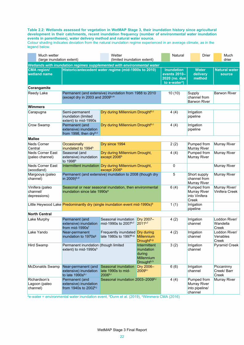
WetMAP Stage 3 Final Report
22
Table 2.2: Wetlands assessed for vegetation in WetMAP Stage 3, their inundation history since agricultural development in their catchments, recent inundation frequency (number of environmental water inundation events in parentheses), water delivery method and natural water source. Colour shading indicates deviation from the natural inundation regime experienced in an average climate, as in the legend below.
Much wetter (large inundation extent)
Wetter (limited inundation extent)
Natural Drier Much drier
Wetlands with inundation regimes supplemented with environmental water CMA region/ wetland name
Historic/antecedent water regime (mid-1900s to 2010) Inundation events 2010–2020 (no. due to e-watera)
Water delivery method
Natural water source
Corangamite
Reedy Lake Permanent (and extensive) inundation from 1988 to 2010 (except dry in 2003 and 2009b,m
10 (10) Supply channel from Barwon River
Barwon River
Wimmera
Carapugna Semi-permanent inundation (limited extent) to mid-1990s
Dry during Millennium Droughtb,c 4 (4) Irrigation pipeline
Crow Swamp Permanent (and extensive) inundation from 1998, then dryb,c
Dry during Millennium Droughtb,c 4 (4) Irrigation pipeline
Mallee
Neds Corner Central
Occasionally inundated to 1994b
Dry since 1994 2 (2) Pumped from Murray River
Murray River
Neds Corner East (paleo channel)
Seasonal (and extensive) inundation to 1998b
Dry during Millennium Drought, except 2006b
4 (4) Pumped from Murray River
Murray River
Neds Corner East (woodland)
Intermittent inundation Dry during Millennium Drought, except 2006b
0
Murray River
Margooya (paleo channel)
Permanent (and extensive) inundation to 2008 (though dry in 2009)b,d
5 Short supply channel from Murray River
Murray River
Vinifera (paleo channel/ depressions)
Seasonal or near seasonal inundation, then environmental inundation since late 1990se
6 (4) Pumped from Murray River into Vinifera Creek
Murray River/ Vinifera Creek
Little Heywood Lake Predominantly dry (single inundation event mid-1990s)b 1 (1) Irrigation pipeline
North Central
Lake Murphy Permanent (and extensive) inundation from mid-1990sf
Seasonal inundation mid-1990s to 2007b,f
Dry 2007– 2011b,f
4 (2) Irrigation channel
Loddon River/ Wandella Creek
Lake Yando Near-permanent inundation to 1970sg
Frequently inundated late 1980s to 1997b,g
Dry during Millennium Droughtb,g
4 (2) Irrigation channel
Loddon River/ Venables Creek
Hird Swamp Permanent inundation (though limited extent) to mid-1990sh
Intermittent inundation during Millennium Droughtb,h
3 (2) Irrigation channel
Pyramid Creek
McDonalds Swamp Near-permanent (and extensive) inundation to late 1990sb,i
Seasonal inundation late 1990s to mid-2006b,i
Dry 2006–2009b,i
6 (6) Irrigation channel
Piccaninny Creek/ Barr Creek
Richardson’s Lagoon (paleo channel)
Permanent (and extensive) inundation from 1940s to 2002b,j
Seasonal inundation 2003–2009b,j 4 (4) Pumped from Murray River into pipeline/ channel
Murray River
ae-water = environmental water inundation event, bDunn et al. (2019), cWimmera CMA (2016)

WetMAP Stage 3 Final Report
23
Table 2.2 (continued)
Much wetter (large inundation extent)
Wetter (limited inundation extent)
Natural Drier Much drier
Wetlands with inundation regimes supplemented with environmental water Wetland Historic/antecedent water regime (mid-1900s to
2010) Inundation
events 2010–2020 (number
due to e-watera)
Water delivery method
Natural water source
Goulburn Broken
Moodie Swamp
Permanent (and extensive) inundation from 1988 to 1995b,k
Seasonal inundation 1995–1998b,k
Mostly dry 1998–2010, during Millennium Droughtb,k
4 (4) Irrigation channels
Broken Creek
Black Swamp
Permanent (and extensive) inundation to 1997b,l
Infrequent inundation during Millennium Droughtb,l
6 (4) Nine Mile Creek/irrigation channel
Nine Mile Creek
Gaynor Swamp
Permanent (and extensive) inundation to 1998b,n
Mostly dry 1998–2010 due to Millennium Droughtb,n
3 (1) Cornella Creek/ irrigation channel
Cornella Creek (from Lake Cooper)
Doctors Swamp
Predominantly seasonal inundation from precipitation run-off from local catchment area. Inundation depth/extent reduced post-1996b,o
8 (1) Irrigation channel
Nearby catchment
Wetlands with natural inundation only Wetland Historic/antecedent water regime (mid-1900s to
2010) Natural inundation events 2010–20
Natural water source
North central
Lake Lalbert Predominantly seasonal inundation from 1988 to 1998b
Dry during Millennium Droughtb
3 Lalbert Creek
Woolshed Swamp
Infrequent inundation 1988 to 1996b
Dry during Millennium Droughtb
2 Local run-off from nearby catchment
Gannawarra Seasonal inundation limited extent 1988 to 2000b
Dry since 2000b 0 Piccaninny Creek/Barr Creek
Tang Tang Swamp
Frequent inundation (long duration) to 1996p
Dry during Millennium Droughtb
3 Bendigo Creek
Goulburn Broken
One Tree Swamp
Predominantly seasonal inundation from 1988 to 2010 (five dry years in this period)b
5 Wanalta Creek
ae-water = environmental water inundation event, bDunn et al. (2019), dMallee CMA (2012), eMallee CMA (2015), fNorth Central CMA (2015a), gNorth Central CMA (2016), hNorth Central CMA (2014a), iNorth Central CMA (2015b), jNorth Central CMA (2014b), kGoulburn Broken CMA (2012b), lGoulburn Broken CMA (2011a), mCorangamite CMA (2017), nGoulburn Broken CMA (2012a), oGoulburn Broken CMA (2011b), pGHD (2011)
Vegetation characteristics of the study wetlands Wetland vegetation was diverse among the study wetlands, and included woodland, shrubland, grassland, herbland and halophytic (saline-tolerant) assemblages (Table 2.3, Figure 2.6). The spatial patterning of these communities is shaped by the wetland’s position in the landscape (riverine floodplain, depressions, coastal), bathymetry (various zones defined by depth and duration of inundation) and climate (semi-arid, temperate).

WetMAP Stage 3 Final Report
24
Table 2.3: Vegetation assemblages among the study wetlands (examples are provided in Figure 2.6). Refer to DELWP (2018) for EVC descriptions.
Structural dominant Vegetation assemblages (EVCs)
Trees Intermittent Swampy Woodland (and complexes) Red Gum Swamp (and complexes) Black Box Wetland Riverine Chenopod Woodland (and temporal mosaics) Lignum Swampy Woodland Riverine Swamp Forest (and complexes)
Shrubs Alluvial Plains Semi-arid Shrubland Brackish Lignum Swamp Lignum Swamp Coastal Hypersaline Saltmarsh
Sedges/grasses Cane Grass Wetland (and complexes) Tall Marsh (and complexes) Spike-sedge Wetland Brackish Wetland Aggregate
Herbs Aquatic Herbland (and complexes) Floodway Pond Herbland (and complexes) Lake Bed Herbland (and complexes) Brackish Aquatic Herbland Brackish Herbland Wet Saltmarsh Herbland
a) b)
Figure 2.6: Study wetlands showing Ecological Vegetation Classes following drawdown. (a) Red Gum Swamp at Doctors Swamp, Goulburn Broken CMA region, and (b) Black Box Wetland at Carapugna, Wimmera CMA region. Marker and measuring tape indicate the transect line in the centre of the vegetation plot.
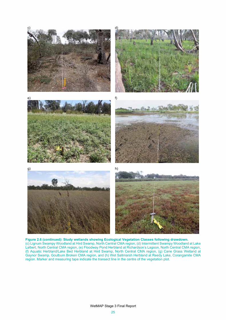
WetMAP Stage 3 Final Report
25
c) d)
e) f)
g) h)
Figure 2.6 (continued): Study wetlands showing Ecological Vegetation Classes following drawdown. (c) Lignum Swampy Woodland at Hird Swamp, North Central CMA region, (d) Intermittent Swampy Woodland at Lake Lalbert, North Central CMA region, (e) Floodway Pond Herbland at Richardson’s Lagoon, North Central CMA region, (f) Aquatic Herbland/Lake Bed Herbland at Hird Swamp, North Central CMA region, (g) Cane Grass Wetland at Gaynor Swamp, Goulburn Broken CMA region, and (h) Wet Saltmarsh Herbland at Reedy Lake, Corangamite CMA region. Marker and measuring tape indicate the transect line in the centre of the vegetation plot.

WetMAP Stage 3 Final Report
26
Survey design Survey timing and treatments Vegetation was assessed within two months following drawdown, which, depending on the timing and magnitude of inundation and the rate of drawdown, varied from late spring to early autumn. Timing of inundation also varied among wetlands. While aiming for inundation over winter and spring, for many wetlands the timing of inundation is dependent on constraints imposed by operation of irrigation networks, the Wimmera–Mallee pipeline, and flows in the Murray River, which collectively provide environmental flows to the study wetlands. For example, no environmental flows are possible in wetlands supplied by irrigation networks between ~15 May and 15 August, when they are closed for channel maintenance. In some wetlands, ‘watering’ (the term often used to describe environmental water inflows and inundation), can commence in late autumn prior to irrigation network seasonal closure. These brief events, often referred to as ‘priming’, saturate wetland soils and minimise losses when watering re-commences in late winter. In other wetlands where such priming is not possible, watering commences in mid-August or sometimes later (for Murray River–supplied wetlands). All wetlands that received environmental water were inundated over spring but may not have been inundated each year. In wetlands that remained dry (i.e. that were not inundated in a particular year), vegetation was assessed in the same period as post drawdown for the inundated wetlands – these samples formed the basis of the dry treatment, used to evaluate the effectiveness of environmental water for KEQs 1–5 (Table 2.4).
The surveys were timed to coincide with maximum expression of wetland species among all groups (aquatic, seasonally inundated, and mudflat; Figure 2.2). Occasionally, it was necessary to visit a wetland twice to follow the drawdown in different zones of the wetland. We considered that a single vegetation assessment in each wetland, each year, in the post-drawdown phase was adequate for addressing the two principal aims: comparing vegetation outcomes between inundated and dry treatments and exploring relationships between vegetation and antecedent hydrology.
Assessments were also undertaken during the inundation phase of several wetlands to provisionally investigate the effect of environmental water ‘top-ups’. These environmental water top-ups represented a second inundation event delivered prior to the drawdown of the first event and were designed to extend the duration of inundation to support waterbird breeding, and duck hunting. These are represented as the ‘inundated’ treatment in Table 2.4.
To determine whether vegetation responses to environmental water inundation differed from responses to natural inundation, we treated them separately in our analyses. Thus, we had four treatments: ‘dry’, ‘inundated’, ‘drawdown – environmental water’, and ‘drawdown – natural inundation’ (Table 2.4).
Table 2.4: Treatments, and their definition in relation to the time of survey.
Wetland inundation treatment Survey timing Conditions
Inundated In between inundation events, surface water present >50% of site inundated
Drawdown – environmental water 1–2 months following drawdown from environmental water No surface water,
soil moist Drawdown – natural inundation 1–2 months following drawdown from natural (unmanaged) inundation
Dry >6 (though mostly >9) months following drawdown Soil dry
Sample stratification and replication To enable investigation of the effects of inundation on the diversity of vegetation types that occur in the study wetlands (Table 2.3), and to accommodate the vegetation community objectives for environmental water in the EWMPs, we stratified sampling by EVCs. Our sampling unit for all KEQs was a 50 x 20 m plot (‘vegetation plot’) with 20 1 x 1 m quadrats arranged either side of a 50 m transect line that ran through the middle of the plot (Figure 2.7). Transects were marked at either end with a permanent marker so they could be located for repeat sampling. Vegetation plots were randomly located within each EVC, and we

WetMAP Stage 3 Final Report
27
placed a minimum of three plots where possible within each EVC in each wetland, as a prior power analysis revealed that a minimum of 60 quadrats were needed to detect changes in vegetation cover with an acceptable degree of confidence (Papas et al. 2018). Plots were divided into 20 x 10 m sections within which woody recruitment counts and lignum condition were assessed.
Figure 2.7: Vegetation plot for assessment of understorey cover and frequency, lignum condition, woody recruitment and tree condition. Each sampling plot includes a centre transect line, 20 nested 1 x 1 m quadrats for understorey floristics, and 10 m sections for lignum cover/condition and woody recruitment counts. Measures collected at each sampling plot included:
species cover in 1 x 1 m quadrats and overhanging canopy cover (where it was within two metres above the ground)
soil moisture (observational) and evidence of recent inundation in every 1 x 1 m quadrat (water depth, proportion of plot inundated)
species not found in the quadrats, but found in the sampling plot lignum cover and condition in each 10 x 20 m section tree counts in each 10 x 20 m section evidence of disturbance (e.g. livestock, horse-riding, carp, vehicles, firewood collection).
Survey methods Species richness and cover (KEQs 1–3, SQs 1–2) Cover/abundance of all plant species, large woody debris (>10 cm diameter), litter, bryophytes/lichens/soil crust and bare ground were assessed by two observers in each 1 x 1 m quadrat in the vegetation plot, using the cover rating categories shown in Appendix 1, Table A1.1. Where dead plant species were identifiable and attached, and not just recently dead annuals, they were recorded as the identified species, assigned a cover value and noted as ‘dead’.
Additionally, a search was conducted in the sampling plot for species not recorded in the 1 x 1 m quadrats to obtain a more comprehensive list of species in the sampling plot, to provide a better estimate of native and exotic species richness for the EVC. This was done by both observers following the assessment of species cover/abundance in the 1 x 1 m quadrats.
Lignum cover, condition (KEQ 4, SQ 4) Lignum cover was measured in each 10 x 20 m section in the sampling plot using the same cover categories as the 1 x 1 m quadrats. Lignum condition metrics followed the method prescribed by Scholz

WetMAP Stage 3 Final Report
28
et al. (2007) and were also measured in each 10 x 20 m section. These included the percentage of viable plant biomass (i.e. not dry/dead), and the colour of the viable crown using the categories in Table A1.2.
At Lake Murphy, soil moisture sensors (90 cm length, Sentek ‘Drill & Drop’) were installed in the lignum root zone to inform the evaluation of the response of lignum to environmental water and antecedent hydrology. Lake Murphy was selected because it has an environmental water objective to rehabilitate the lignum that fringes parts of the wetland (North Central CMA 2015a), but plants are not inundated by environmental water as this zone is slightly elevated. We were interested in whether the water (~20 m away from the plants) would move (i.e. wick up) through the soil. Two sensors were installed immediately adjacent to a group of plants, with one positioned slightly down-slope of the other (at 60 cm lower elevation than the first), so that between the two sensors, we would have data for between 5 and 150 cm depth. Data were recorded between December 2018 and January 2020. These data were plotted to visually examine moisture trends at different depths.
Tree life stages and counts (KEQ 5)
In EVCs where woody vegetation was a component of the vegetation assemblage (e.g. Black Box Wetland, Intermittent Swampy Woodland, Lignum Swampy Woodland, Red Gum Swamp, Riverine Swamp Forest and their complexes), the abundances by life stages of River Red Gum and Black Box were determined by counting the number of individuals of each life stage class (Table A1.3) in each 10 x 20 m section in the sampling plot.
Condition of individual trees (KEQ 6)
Measures of growth and reproduction that collectively provide an indication of tree condition (Souter et al. 2012) were made at 30 randomly selected and permanently marked mature and old mature trees (i.e. trees with a trunk diameter at 1.3 m height (DBH) greater than 10 cm). These were located in or immediately adjacent to the sampling plots. Measures included:
DBH crown extent new tip growth extent of reproduction.
Trunk diameter and crown extent were measured at the beginning and end of this WetMAP stage (2017–2018 and 2019–2020, respectively) rather than in each survey, as they are not expected to change significantly in this time frame. The extent of the tree crown is defined as the proportion of the tree with live foliage (recorded to the nearest 5%). Growth of new shoots from branch tips and the relative abundance of buds, flowers and fruit (i.e. the extent of reproduction) are expected to respond over shorter time frames and were assessed each year. These were assessed visually and recorded using the categories in Tables A1.4 and A1.5, respectively.
Tall native herbaceous vegetation (SQ 7)
Due to their great height and density, these plants are difficult to survey on the ground. Thus, the areal extent of Cumbungi (Typha spp.) and Common Reed (Phragmites australis) patches (collectively known as Tall Marsh), in wetlands where these species are present, was mapped by collecting images from a remotely piloted aircraft and stitching these together into a single image using image editing software. This work was undertaken by Australian UAV. Boundaries and the extent of Tall Marsh were determined by expert visual assessment assisted by GIS software. An initial assessment of the rates of colonisation indicated that an assessment every three years is appropriate for detecting changes in extent. Aerial image collection is scheduled every three years, and the first iteration of images and maps was generated in autumn 2019. An assessment of this SQ cannot be undertaken in this stage of the study, as data from the second iteration planned for 2022 are required in order to examine change.
Data analysis First, we summarised broad characteristics of the wetland vegetation to provide an overview of the composition of wetland, terrestrial and dampland species recorded in the study, their origin (native or
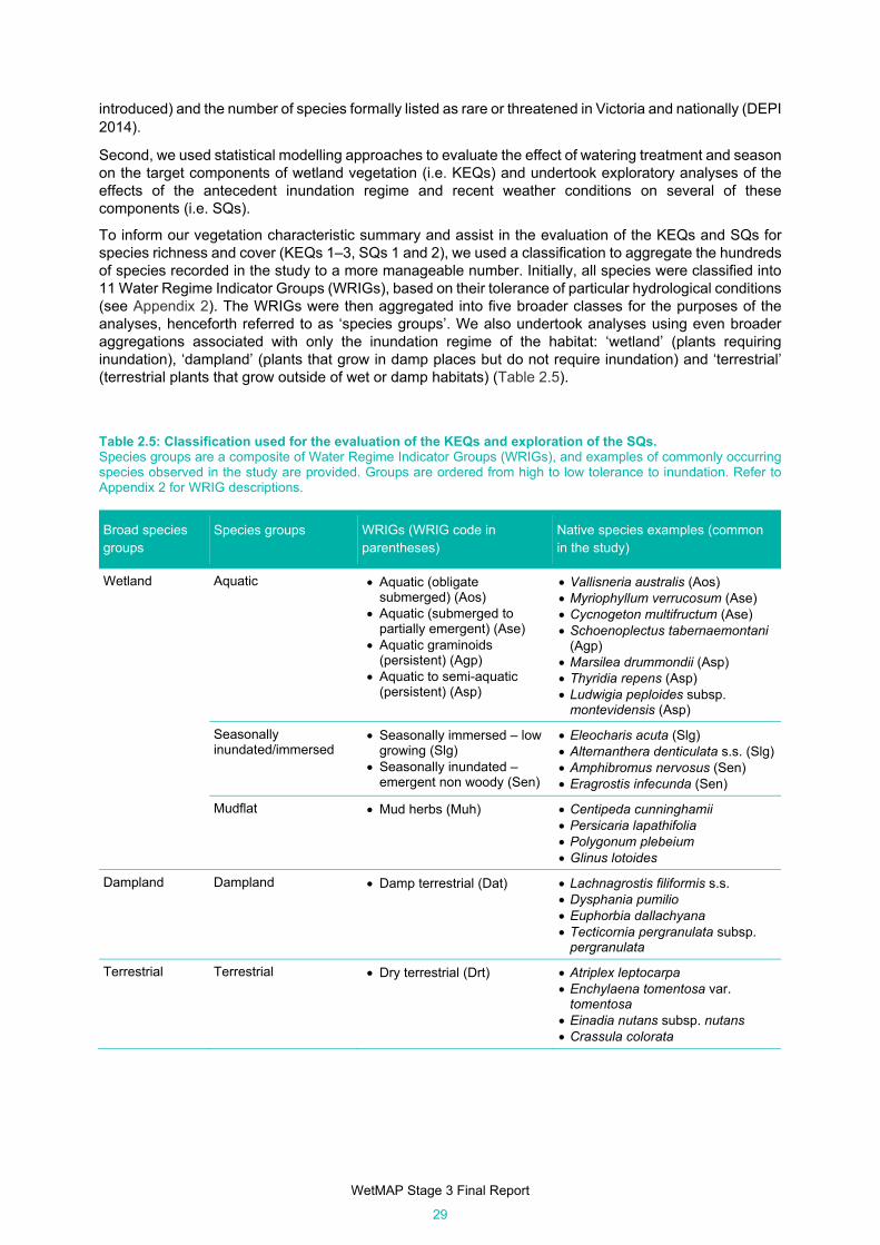
WetMAP Stage 3 Final Report
29
introduced) and the number of species formally listed as rare or threatened in Victoria and nationally (DEPI 2014).
Second, we used statistical modelling approaches to evaluate the effect of watering treatment and season on the target components of wetland vegetation (i.e. KEQs) and undertook exploratory analyses of the effects of the antecedent inundation regime and recent weather conditions on several of these components (i.e. SQs).
To inform our vegetation characteristic summary and assist in the evaluation of the KEQs and SQs for species richness and cover (KEQs 1–3, SQs 1 and 2), we used a classification to aggregate the hundreds of species recorded in the study to a more manageable number. Initially, all species were classified into 11 Water Regime Indicator Groups (WRIGs), based on their tolerance of particular hydrological conditions (see Appendix 2). The WRIGs were then aggregated into five broader classes for the purposes of the analyses, henceforth referred to as ‘species groups’. We also undertook analyses using even broader aggregations associated with only the inundation regime of the habitat: ‘wetland’ (plants requiring inundation), ‘dampland’ (plants that grow in damp places but do not require inundation) and ‘terrestrial’ (terrestrial plants that grow outside of wet or damp habitats) (Table 2.5).
Table 2.5: Classification used for the evaluation of the KEQs and exploration of the SQs. Species groups are a composite of Water Regime Indicator Groups (WRIGs), and examples of commonly occurring species observed in the study are provided. Groups are ordered from high to low tolerance to inundation. Refer to Appendix 2 for WRIG descriptions.
Broad species groups
Species groups WRIGs (WRIG code in parentheses)
Native species examples (common in the study)
Wetland Aquatic Aquatic (obligate submerged) (Aos)
Aquatic (submerged to partially emergent) (Ase)
Aquatic graminoids (persistent) (Agp)
Aquatic to semi-aquatic (persistent) (Asp)
Vallisneria australis (Aos) Myriophyllum verrucosum (Ase) Cycnogeton multifructum (Ase) Schoenoplectus tabernaemontani
(Agp) Marsilea drummondii (Asp) Thyridia repens (Asp) Ludwigia peploides subsp.
montevidensis (Asp)
Seasonally inundated/immersed
Seasonally immersed – low growing (Slg)
Seasonally inundated – emergent non woody (Sen)
Eleocharis acuta (Slg) Alternanthera denticulata s.s. (Slg) Amphibromus nervosus (Sen) Eragrostis infecunda (Sen)
Mudflat Mud herbs (Muh) Centipeda cunninghamii Persicaria lapathifolia Polygonum plebeium Glinus lotoides
Dampland Dampland Damp terrestrial (Dat) Lachnagrostis filiformis s.s. Dysphania pumilio Euphorbia dallachyana Tecticornia pergranulata subsp.
pergranulata
Terrestrial Terrestrial Dry terrestrial (Drt) Atriplex leptocarpa Enchylaena tomentosa var.
tomentosa Einadia nutans subsp. nutans Crassula colorata

WetMAP Stage 3 Final Report
30
Selection of independent variables used in analyses Predictor variables used in our models (Table 2.6) were those that have been identified as important drivers of vegetation responses to the inundation regime and recent weather conditions (see Section 2.1.2). Key reviews and studies that informed these variables were: Casanova and Brock (2000) and Altenfelder et al. (2016) for wetland species richness and cover responses; Frood and Papas (2016), Craig et al. (1991), Overton et al. (2014) and Freestone et al. (2017) for lignum responses; and Jensen et al. (2007) and Moxham et al. (2018) for River Red Gum and Black Box tip growth and flowering responses.
Hydrology variables were derived from the Geoscience Australia ‘Wetland Insights Tool’ (WIT) models (Dunn et al. 2019). The tool is based on algorithms that detect the presence of water from Landsat data (refer to Appendix 3 for further details). We obtained the relevant data at our vegetation plot scale, and to ensure that at least one Landsat pixel (30 x 30 m) fell inside our plots, we added a 5 m buffer (i.e. 55 x 25 m). We validated the outputs for every plot by comparing the WIT output with our field observations (between 2017 and 2020) and Google Earth aerial imagery (between 2010 and 2020). WIT data for plots in two wetlands (Margooya and Carapugna) did not accurately reflect the inundation experienced in these plots, because the dry plots in Margooya are very close to permanent water and the data are showing the presence of water in the dry plots, and because the plots in Carapugna are among large Black Box trees, which have prevented detection of water. Affected plots from these wetlands were omitted from the analyses.
Weather variables (mean maximum temperature and rainfall in the three months prior to the survey) for each wetland were derived from data obtained from the Bureau of Meteorology for the station located closest to the wetland.

WetMAP Stage 3 Final Report
31
Table 2.6: Response variables, and independent variables identified as important drivers of wetland vegetation responses, for evaluation of the KEQs and SQs evaluated in Stage 3. Wetland inundation treatments are: inundated, drawdown – environmental water, drawdown – natural inundation and dry (see Table 2.4 for details).
Questions Response variables Predictor variables
KEQ 1: Do environmental water events increase native wetland plant species richness?
Total native wetland1 species richness
Total native aquatic2 species richness
Total native mudflat3 species richness
Total native seasonally inundated/immersed4 species richness
Total native dampland5 species richness
Season (Aug–Nov, Dec–Feb, Mar–May) Inundation treatment (Table 2.3)
SQ 1: How does the antecedent water regime affect native wetland plant species richness?
Time since inundation7 Duration of most recent inundation event Total rainfall three months prior Mean maximum temperature three months
prior Total number of inundation events in prior
decade8 Duration of inundation in the decade prior
KEQ 2: Do environmental water events increase the cover of native wetland plant species?
Native wetland cover Native aquatic cover Native mudflat cover Native seasonally
inundated/immersed cover
Season (Aug–Nov, Dec–Feb, Mar–May) Inundation treatment (Table 2.3)
SQ 2: How does antecedent water regime affect the cover of native wetland plant species?
Time since inundation7 Duration of most recent inundation event Total rainfall three months prior Mean maximum temperature three months
prior Duration of inundation in decade prior
KEQ 3: Do environmental water events reduce the cover of terrestrial plant species in wetlands?
Cover of native terrestrial species6
Cover of introduced terrestrial species6
Season (Aug–Nov, Dec–Feb, Mar–May) Inundation treatment (Table 2.3)
KEQ 4: Do environmental water events improve the condition of lignum in wetlands?
Lignum condition score Season (Aug–Nov, Dec–Feb, Mar–May) Inundation treatment (Table 2.3)
SQ 4: How does the antecedent water regime affect the condition of lignum in wetlands?
Time since inundation Total duration of inundation in prior
decade Total rainfall decade prior Total duration of inundation three decades
prior
KEQ 5: Do environmental water events lead to growth and flowering of mature wetland tree species?
Tip growth score River Red Gum
Tip growth score Black Box Flowering score River Red
Gum Flowering score Black Box
Inundation treatment (Table 2.3) Total rainfall three months prior Mean maximum temperature three months
prior
KEQ 6: Did environmental water support survival of mature trees?
Abundance of mature9 trees Not applicable
1 All WRIGs except Dat/Drt, 2 WRIGs: Aos/Ase/Agp/Asp, 3 WRIG: Muh, 4 WRIG: Slg/Sen, 5 WRIG: Dat, 6 WRIG: Drt, 7 Inundation event ≥15% inundation extent, 30-day duration, 8 60 days between events, 9 See Appendix 1, Table A1.3 for criteria that define tree life stage classes.

WetMAP Stage 3 Final Report
32
Analysis approach
KEQ 1: Do environmental water events increase native wetland plant species richness?
We used generalised Poisson linear mixed models (implemented with the glmer function from the lme4 package in R; R Core Team 2020, Bates et al. 2015) to explore the relationships between each of the five response variables (species richness of the various groups) and the two independent variables (inundation treatment and season) (Table 2.6). We included sampling year and vegetation plot nested within wetland as random effects. We examined residual plots for all models and extracted predictions (using the emmeans package) to demonstrate relationships. As the data are unbalanced, coefficients (the difference in the intercepts for each treatment) are presented as model outputs, whereas the figures present predicted values derived from the models (i.e. estimated marginal means).
To inspect variation among wetlands, we calculated the mean native total wetland species richness of each wetland for two inundation treatments: dry and drawdown (either following environmental water or natural inundation). To assist with interpretation of high species richness in the dry treatment in some wetlands, we also calculated the contribution of each wetland species group (aquatic, seasonally inundated/immersed, mudflat) to the mean native wetland species richness for this treatment (using the emmeans function to extract means from glmer).
SQ 1: How does antecedent water regime affect native wetland plant species richness?
We explored relationships between hydrological and weather variables and the five vegetation response variables (Table 2.6). The method of analysis differed for each vegetation response variable. For native total wetland species richness, we used generalised additive mixed models (GAMMs), with wetland and plot nested within wetland as random effects (implemented with the gamm4 package in R; R Core team 2020, Wood and Scheipl 2020). We ran separate models examining the effects of each predictor on richness (log-transformed to improve normality). We compared model fits using Akaike’s Information Criteria corrected for small sample sizes. The best predictor for total species richness was time since inundation, but the distribution of data did not allow us to test for seasonal trends. In addition, the available data did not span the entire range of days since inundation very well (see Figure 2.8). We therefore also ran a second analysis comparing richness across time since inundation, split into five groups: 0 (i.e. currently inundated), 1–500, 501–1000, 1001–5000 and >5000 days since inundation. This model was fitted as a linear mixed-effects model, with wetland and plot nested within wetlands as random effects, as above.
Figure 2.8: Histogram showing distribution of samples with various times since inundation. For dampland and seasonally inundated species richness, we were able to successfully fit the GAMM outlined above, except for using a negative binomial rather than a Gaussian distribution.
Aquatic species richness had many zero observations. We therefore ran a series of zero-inflated mixed-effects models (using functions from the glmmTMB package in R; R Core Team 2020, Brooks et al. 2017) to explore the influence of each predictor on this variable. Time since inundation was not included,
Cou
nt

WetMAP Stage 3 Final Report
33
because models for this variable would not converge. Wetland and sampling plot nested within wetland were included as random effects, and a negative binomial distribution was used.
Nearly 70% of observations of mudflat species richness were either zero or one. We therefore converted all observations to presence/absence data (i.e. zero values were kept as zero, any value >1 was converted to 1). We then fitted a logistic regression model for three variables: number of inundation events in the previous decade, temperature, and rainfall (models for other variables would not converge). This model included wetland as a random effect and used a binomial distribution. All three variables were influential predictors, so we then fitted models with the number of inundation events and either rainfall or temperature, and a final model with all three variables. We selected the best model based on Akaike’s Information Criteria, as above.
KEQs 2 and 3: Do environmental water events increase the cover of native wetland plant species (KEQ 2) and do environmental water events reduce the cover of terrestrial plant species in wetlands (KEQ 3)?
We used an ordinal (cumulative link) mixed-effects model (using the clmm function in the ordinal package in R; R Core Team 2020, Christensen 2019) to explore the relationship between each of the four response variables (KEQ 2) or two response variables (KEQ 3) and the two independent variables (inundation treatment and season) (Table 2.6). We used this model because it is more straightforward to run (on ordered cover categories), than a beta hurdle model approach and allows an understanding of how different cover categories are affected by treatment and season. It also allows for repeated measures data, accounting for the fact that multiple responses from the same wetland or sampling year are likely to be more similar than responses from other plots. However, cumulative link models for ordinal regression use non-linear link functions, and consequently model parameters are not as simple to interpret as for generalised linear regression. Instead, we have taken the approach of reporting effects on a probability scale, rather than on the scale of the link function. We examined residual plots for all models and extracted predictions (using the ggeffects package) for clmm to demonstrate relationships.
To inspect variation among wetlands, we calculated and plotted the mean native wetland and terrestrial species cover of each wetland for two principal inundation treatments: dry and drawdown, where drawdown was from either environmental water or natural inundation. To assist with interpretation of the high cover of native wetland species in the dry treatment, in some wetlands we also calculated the contribution of each wetland species group (aquatic, seasonally inundated/immersed, mudflat) to the mean wetland species cover for this treatment.
SQ 2: How does antecedent water regime affect the cover of native wetland plant species?
We explored relationships between hydrological and weather variables and the four vegetation response variables (Table 2.6). For native total wetland cover and seasonally inundated/immersed species cover, we used GAMMs, with wetland and plot nested within wetland as random effects (implemented with the gamm4 package in R; R Core team 2020, Wood and Scheipl 2020). Not all wetlands were sampled in all years, so year was not included as a random effect. We compared model fits for models built with different hydrological and weather variables using Akaike’s Information Criteria corrected for small sample sizes. For aquatic and mudflat species cover, due to the large number of zero observations, the data were split into two components; non-zero data only (conditional model using GAMM) and binary presence/absence data, to simulate a hurdle model/zero-inflated approach that meets the issues of zero-inflation. Binary models were run using glmer from the lme4 package in R (R Core Team 2020, Bates et al. 2015).
KEQ 4: Do environmental water events improve the condition of lignum in wetlands?
We used a linear mixed model (implemented with the lmer function from the lme4 package in R; R Core Team 2020, Bates et al. 2015) to explore relationships between the response variable (lignum condition) and independent variables (treatment and season) (Table 2.6). This modelling approach was used because it takes into account that multiple responses from the same plot (or wetland or sampling year) may be more similar than responses from other plots. We examined residual plots for all models and extracted predictions (using the emmeans function) to extract means from lmer to demonstrate relationships.

WetMAP Stage 3 Final Report
34
To inspect variation among wetlands, we calculated the mean lignum condition score for each wetland for two principle inundation treatments: dry and drawdown (from environmental water or natural inundation).
SQ 4: How does the antecedent water regime affect the condition of lignum in wetlands?
We explored the relationship between lignum condition scores and four independent variables (Table 2.6). Two of these (total days inundated in the previous decade and duration of inundation over the past 30 years) were highly correlated (Pearson’s r = 0.91), so only the former was used. We fitted a GAMM (implemented with the gamm4 package in R; R Core team 2020, Wood and Scheipl 2020) between lignum condition and each predictor individually, along with a null (intercept-only) model. These models had wetland and year included as random effects. We then ran a final model with the two best predictors. We used Akaike’s Information Criteria to compare models, and we present predictions from the best one. Model assumptions were assessed as per other mixed-effects models in this chapter. Residual plots for all models were examined and predictions extracted to demonstrate relationships.
KEQ 5: Do environmental water events lead to growth and flowering of mature wetland tree species?
We used ordinal regression (implemented with the clmm function from the ordinal package in R; R Core Team 2020, Christensen 2019) to test whether the tip growth and flowering scores for River Red Gum and Black Box varied in relation to hydrological treatment, rainfall and temperature in the previous three months (Table 2.6). We ran an individual model for each species and their separate responses (i.e. four models in total) that included the hydrological treatment, rainfall and temperature as two fixed factors; Wetland was included as a random effect. We were interested primarily in testing for differences between hydrological treatments and exploring the additional effects of temperature and rainfall. Given that the aim was not to explore interactions between treatment and the two weather variables, the model was additive (i.e. Response = Hydrological Treatment + Rainfall + Temperature). We extracted model predictors for statistically significant variables based on the mean values of rainfall and temperature, and for the drawdown environmental water treatment. Only three trees from one site were observed in the ‘Drawdown natural inundation’ treatment for Black Box tip growth and flowering, so they were removed from the dataset before analysis.
KEQ 6: Did environmental water support survival of mature trees?
Survival of mature Black Box and River Red Gum trees was determined by comparing the number of living mature trees in the first and last surveys in each wetland with trees (Table 2.6). This included trees in the vegetation sampling plots in addition to trees outside the sampling plots that were assessed for tip growth and flowering.
Sample sizes for treatments For species richness and cover KEQs/SQs (1–3), we had 477 samples among 22 wetlands, and 159 samples for lignum among 14 wetlands (KEQ/SQ 4) available for use in the analyses. A total of 729 River Red Gum trees and 352 Black Box samples (individual trees assessed multiple times) were assessed for KEQ 5. KEQ 6 compared the total number of trees of each species between the first and last survey (Table 2.7).

WetMAP Stage 3 Final Report
35
Table 2.7: Sample sizes for inundation treatments for each KEQ and SQ. RRG = River Red Gum, BB = Black Box.
Key Evaluation Question Total number of samples with number of wetlands in parentheses
Number of samples in each treatment
Dry Inundated Drawdown – environmental water
Drawdown –natural inundation
KEQ 1/SQ 1: Native wetland plant species richness
477 (22) 294 22 142 19
KEQ 2/ SQ 2: Native wetland plant species cover
KEQ 3: Terrestrial plant species cover
KEQ 4: Lignum condition 159 (14) 118 12 25 4 (too few to include in analyses)
KEQ 5: Growth and flowering of mature trees
7291 RRG 3521 BB (15)
5831 RRG 2801 BB
0 771 RRG 721 BB
691 RRG 0 BB
KEQ 6: Survival of mature trees
590 RRG 949 BB (10)
Comparison of tree mortality/survivorship among all wetlands between first and last survey
1 Individual trees sampled on multiple occasions.
Results
Summary of vegetation characteristics among surveys and wetlands Among all sites and surveys (501 samples in total), 595 species were recorded. Of these, 374 (63%) were native and 221 (37%) introduced. Of the native species, 188 (51%) were wetland species (plants requiring inundation), 94 (25%) dampland species (plants preferring moist environments but not requiring inundation) and 92 (24%) terrestrial species (terrestrial plants that grow outside of wet or damp habitats). There were far fewer introduced wetland species than introduced terrestrial species. The dampland native species Common Blown-grass (Lachnagrostis filiformis s.s.) was the most common plant among survey plots and occurred at the highest cover. Following this, native wetland species ranked highest for their cover, but several introduced terrestrial species ranked highly for their frequency of occurrence (Table 2.8a). Considering wetland species only, the native plants Southern Cane-grass (Eragrostis infecunda), Tangled Lignum and Red Water-milfoil (Myriophyllum verrucosum) had the highest cover among the sampling plots, and Common Spike-sedge (Eleocharis acuta), Common Sneezeweed (Centipeda cunninghamii) and Lesser Joyweed (Alternanthera denticulata s.s.) the highest frequency of occurrence among the sampling plots. Only two introduced species were in the top-10-ranked commonly occurring wetland plants: Curled Dock (Rumex crispus ) and Creeping Heliotrope (Heliotropium supinum) (Table 2.8b).
Sixty species formally listed as rare or threatened in Victoria, and four nationally (DEPI 2014), were recorded in 19 of 22 wetlands among all surveys. Most of these (62%) were wetland species (Figure 2.9). The majority (88%) of the records of these species were from six wetlands (Margooya, Neds Corner Central, Lake Lalbert, Carapugna, Little Lake Heywood and Neds Corner East) (Appendix 4).

WetMAP Stage 3 Final Report
36
Figure 2.9: Total numbers of terrestrial, dampland and wetland species recorded among all surveys and wetlands, and the proportions of native, introduced and threatened species.
0
50
100
150
200
250
300
Terrestrial Dampland Wetland
Num
ber
of s
peci
es
Species group
Native Threatened species Introduced
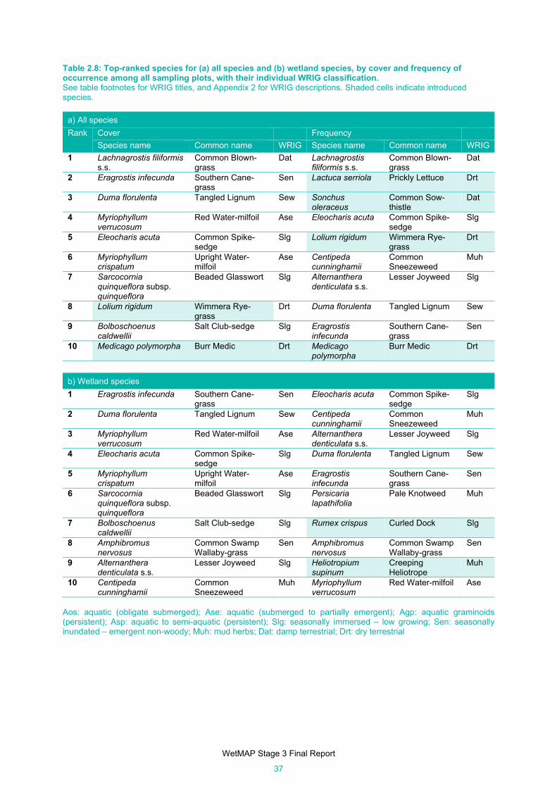
WetMAP Stage 3 Final Report
37
Table 2.8: Top-ranked species for (a) all species and (b) wetland species, by cover and frequency of occurrence among all sampling plots, with their individual WRIG classification. See table footnotes for WRIG titles, and Appendix 2 for WRIG descriptions. Shaded cells indicate introduced species.
a) All species
Rank Cover Frequency
Species name Common name WRIG Species name Common name WRIG
1 Lachnagrostis filiformis s.s.
Common Blown-grass
Dat Lachnagrostis filiformis s.s.
Common Blown-grass
Dat
2 Eragrostis infecunda Southern Cane-grass
Sen Lactuca serriola Prickly Lettuce Drt
3 Duma florulenta Tangled Lignum Sew Sonchus oleraceus
Common Sow-thistle
Dat
4 Myriophyllum verrucosum
Red Water-milfoil Ase Eleocharis acuta Common Spike-sedge
Slg
5 Eleocharis acuta Common Spike-sedge
Slg Lolium rigidum Wimmera Rye-grass
Drt
6 Myriophyllum crispatum
Upright Water-milfoil
Ase Centipeda cunninghamii
Common Sneezeweed
Muh
7 Sarcocornia quinqueflora subsp. quinqueflora
Beaded Glasswort Slg Alternanthera denticulata s.s.
Lesser Joyweed Slg
8 Lolium rigidum Wimmera Rye-grass
Drt Duma florulenta Tangled Lignum Sew
9 Bolboschoenus caldwellii
Salt Club-sedge Slg Eragrostis infecunda
Southern Cane-grass
Sen
10 Medicago polymorpha Burr Medic Drt Medicago polymorpha
Burr Medic Drt
b) Wetland species
1 Eragrostis infecunda Southern Cane-grass
Sen Eleocharis acuta Common Spike-sedge
Slg
2 Duma florulenta Tangled Lignum Sew Centipeda cunninghamii
Common Sneezeweed
Muh
3 Myriophyllum verrucosum
Red Water-milfoil Ase Alternanthera denticulata s.s.
Lesser Joyweed Slg
4 Eleocharis acuta Common Spike-sedge
Slg Duma florulenta Tangled Lignum Sew
5 Myriophyllum crispatum
Upright Water-milfoil
Ase Eragrostis infecunda
Southern Cane-grass
Sen
6 Sarcocornia quinqueflora subsp. quinqueflora
Beaded Glasswort Slg Persicaria lapathifolia
Pale Knotweed Muh
7 Bolboschoenus caldwellii
Salt Club-sedge Slg Rumex crispus Curled Dock Slg
8 Amphibromus nervosus
Common Swamp Wallaby-grass
Sen Amphibromus nervosus
Common Swamp Wallaby-grass
Sen
9 Alternanthera denticulata s.s.
Lesser Joyweed Slg Heliotropium supinum
Creeping Heliotrope
Muh
10 Centipeda cunninghamii
Common Sneezeweed
Muh Myriophyllum verrucosum
Red Water-milfoil Ase
Aos: aquatic (obligate submerged); Ase: aquatic (submerged to partially emergent); Agp: aquatic graminoids (persistent); Asp: aquatic to semi-aquatic (persistent); Slg: seasonally immersed – low growing; Sen: seasonally inundated – emergent non-woody; Muh: mud herbs; Dat: damp terrestrial; Drt: dry terrestrial

WetMAP Stage 3 Final Report
38
Responses of understorey vegetation to inundation and environmental water (KEQs 1–3, SQ 1)
KEQ 1: Do environmental water events increase native wetland plant species richness?
Total native wetland species richness
The mean native wetland species richness at the sampling plots scale (i.e. number of species among all wetland species groups in each sampling plot) was significantly higher in all drawdown and inundated treatments than in dry treatments (Appendix 5, Table A5.1), by 1.42 additional species [95% CI (1.17, 1.65)] in the drawdown (natural inundation) treatment, 1.7 species [95% CI (1.53, 1.91)] in the drawdown (environmental water inundation) treatment and 1.6 species [95% CI (1.28, 1.86)] in the inundated (environmental water treatment) (Figure 2.10, Table 2.9, Appendix 5, Table A5.1). In addition, native wetland species richness was significantly lower in summer and autumn than in spring, by 1.2 species [95% CI (1.31, 1.04)] in summer than in spring, and by 1.4 species [95% CI (1.64, 1.36)] in autumn than in spring (Figure 2.10, Table 2.9). The estimated among-site (wetland) standard deviation was 1.99, meaning that sites varied substantially in their species richness relative to treatments (Figure 2.10).
Aquatic species
Aquatic species richness was significantly higher in all drawdown and inundated treatments than in the dry treatment (Appendix 5, Table A5.1), by 3.2 species [95% CI (2.07, 4.82)] in the drawdown (natural inundation) treatment, by 4.3 species [95% CI (3.21, 5.69)] in the drawdown (environmental water inundation) treatment and by 5.8 species [95% CI (3.94, 8.49)] in the inundated (environmental water treatment) (Figure 2.10, Table 2.9).The estimated among-site (wetland) standard deviation was 2.37, meaning that sites varied in their species richness relative to the variation between treatments.
Seasonally inundated/immersed species
Seasonally inundated species richness was significantly higher in in the drawdown (environmental water inundation) treatment than in the dry treatment (Appendix 5, Table A5.1), by 1.3 species [95% CI (1.07, 1.49)]. There were no significant differences in species richness between the drawdown (natural inundation) treatment and the dry treatment and the inundated (environmental water) treatment and the dry treatment. Species richness was also significantly lower in autumn than spring, by 1.4 [95% CI (1.64, 1.12)] species but no different in summer (Figure 2.10, Table 2.9). The estimated among-site (wetland) standard deviation was 1.90, meaning that the variation in species richness was high among sites relative to the variation among treatments.
Mudflat species
Mudflat species richness was significantly higher in the drawdown (environmental water inundation) treatment than in the dry treatment (Appendix 5, Table A5.1), by 2.38 species [95% CI (1.90, 2.97)]. In addition, species richness was significantly lower in summer and autumn than in spring, by 1.6 [95% CI (2.11, 1.20)] species in summer and by 1.9 [95% CI (2.41, 1.42)] species in autumn (Figure 2.10, Table 2.9). The estimated between-site (wetland) standard deviation was 3.2, meaning that sites varied in their species richness relative to variation between treatments.
2 Note that all values are reported coefficients that represent the difference in the intercepts for each treatment.
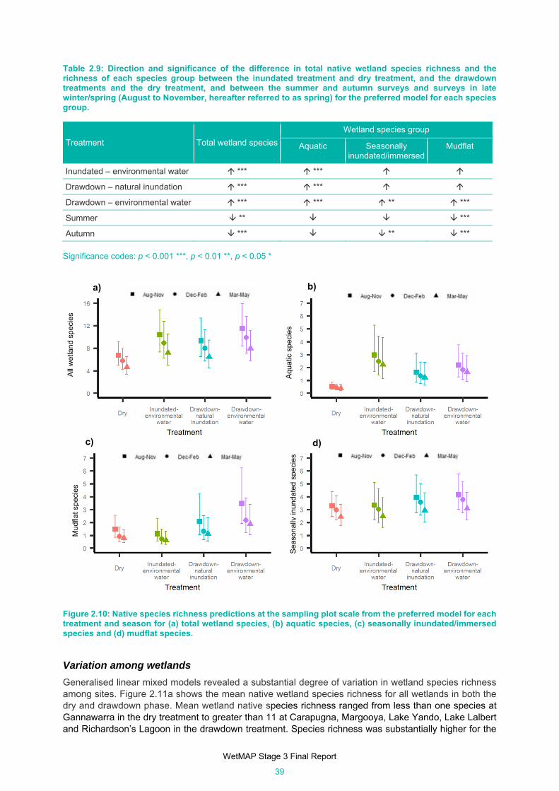
WetMAP Stage 3 Final Report
39
Table 2.9: Direction and significance of the difference in total native wetland species richness and the richness of each species group between the inundated treatment and dry treatment, and the drawdown treatments and the dry treatment, and between the summer and autumn surveys and surveys in late winter/spring (August to November, hereafter referred to as spring) for the preferred model for each species group.
Treatment Total wetland species
Wetland species group
Aquatic Seasonally inundated/immersed
Mudflat
Inundated – environmental water *** ***
Drawdown – natural inundation *** ***
Drawdown – environmental water *** *** ** ***
Summer ** ***
Autumn *** ** ***
Significance codes: p < 0.001 ***, p < 0.01 **, p < 0.05 *
Figure 2.10: Native species richness predictions at the sampling plot scale from the preferred model for each treatment and season for (a) total wetland species, (b) aquatic species, (c) seasonally inundated/immersed species and (d) mudflat species.
Variation among wetlands
Generalised linear mixed models revealed a substantial degree of variation in wetland species richness among sites. Figure 2.11a shows the mean native wetland species richness for all wetlands in both the dry and drawdown phase. Mean wetland native species richness ranged from less than one species at Gannawarra in the dry treatment to greater than 11 at Carapugna, Margooya, Lake Yando, Lake Lalbert and Richardson’s Lagoon in the drawdown treatment. Species richness was substantially higher for the
a) b)
c) d)
All
wet
land
spe
cies
Aqu
atic
spe
cies
Mud
flat s
peci
es
Sea
sona
lly in
unda
ted
spe
cie
s
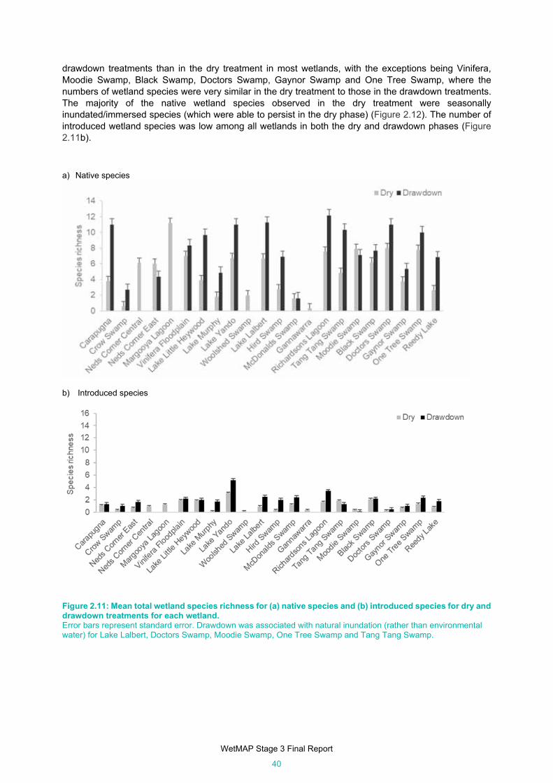
WetMAP Stage 3 Final Report
40
drawdown treatments than in the dry treatment in most wetlands, with the exceptions being Vinifera, Moodie Swamp, Black Swamp, Doctors Swamp, Gaynor Swamp and One Tree Swamp, where the numbers of wetland species were very similar in the dry treatment to those in the drawdown treatments. The majority of the native wetland species observed in the dry treatment were seasonally inundated/immersed species (which were able to persist in the dry phase) (Figure 2.12). The number of introduced wetland species was low among all wetlands in both the dry and drawdown phases (Figure 2.11b).
a) Native species
b) Introduced species
Figure 2.11: Mean total wetland species richness for (a) native species and (b) introduced species for dry and drawdown treatments for each wetland. Error bars represent standard error. Drawdown was associated with natural inundation (rather than environmental water) for Lake Lalbert, Doctors Swamp, Moodie Swamp, One Tree Swamp and Tang Tang Swamp.

WetMAP Stage 3 Final Report
41
Figure 2.12: Native total wetland species richness for the dry treatment, showing the contribution from each species group.
SQ 1: How does the antecedent water regime affect native wetland plant species richness? Total native species richness was best predicted by time since inundation (Appendix 5, Table A5.2). At sites that were currently inundated (time since inundation = 0), nearly 10 species were predicted by the GAMM to be present, in comparison with 4 at sites that hadn’t been inundated for more than 5000 days; this result varied between the GAMM (Figure 2.13a) and the linear mixed-effects model (Figure 2.13b) in the time since inundation period 1–500 days. However, while both results were statistically significant, the relationships were quite variable (R2 for both models was only ~0.11).
The best predictor of aquatic species richness was the total duration of inundation in the prior decade (Appendix 5, Table A5.2). At sites with no inundation, fewer than one aquatic species was predicted; at sites that had been inundated for more than 3000 days in the prior decade, ~4 species were predicted (Figure 2.14a). It should be noted, however, that the reliability of these predictions at the upper end of inundation duration is affected by the lack of vegetation data from high antecedent inundation contexts.
While the number of dampland species was also best predicted by the total duration of inundation in the prior decade (Appendix 5, Table A5.2), the trend was in the opposite direction: >3 species were predicted to occur at sites with no inundation, but close to zero species were predicted at sites inundated for >300 days (Figure 2.14b). This relationship was also quite variable (R2 for the dampland model = 0.13). None of the environmental variables was a significantly better predictor of richness of seasonally inundated species than the null (intercept-only) model (Appendix 5, Table A5.2). The best model for mudflat species richness included three predictors (number of inundation events in the prior decade, mean of the daily maximum temperature in the three months prior, and total rainfall in the three months prior) (Appendix 5, Table A5.2), but the model with the number of inundation events in the decade prior and mean maximum daily temperatures in the past three months was comparable (delta Akaike information criterion <2 units lower; Appendix 5, Table A5.2). This model showed the probability of occurrence of mudflat species was highest when wetlands were inundated more frequently (Figure 2.15a), and when the maximum daily temperature was lower (Figure 2.15b).
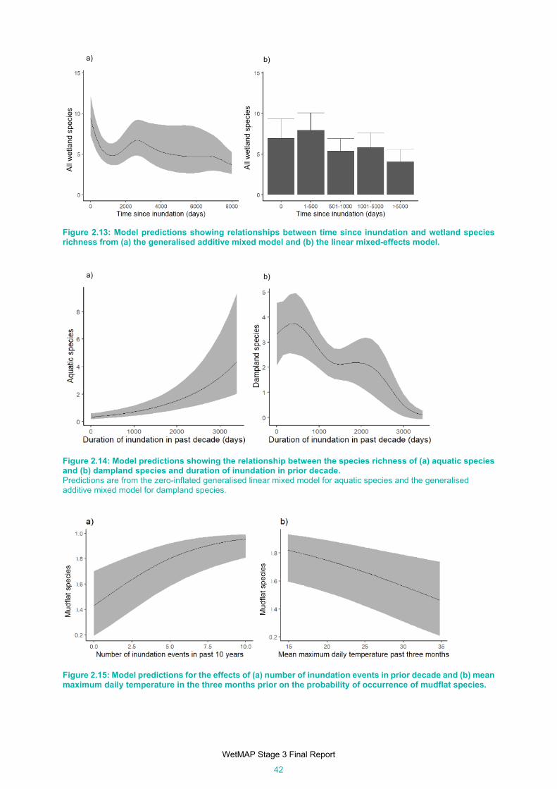
WetMAP Stage 3 Final Report
42
Figure 2.13: Model predictions showing relationships between time since inundation and wetland species richness from (a) the generalised additive mixed model and (b) the linear mixed-effects model.
Figure 2.14: Model predictions showing the relationship between the species richness of (a) aquatic species and (b) dampland species and duration of inundation in prior decade. Predictions are from the zero-inflated generalised linear mixed model for aquatic species and the generalised additive mixed model for dampland species.
Figure 2.15: Model predictions for the effects of (a) number of inundation events in prior decade and (b) mean maximum daily temperature in the three months prior on the probability of occurrence of mudflat species.
a) b)
Mud
flat s
peci
es
Mud
flat s
peci
es
a) b) A
ll w
etla
nd s
peci
es
All
wet
land
spe
cies

WetMAP Stage 3 Final Report
43
KEQ 2: Do environmental water events increase the cover of native wetland plant species?
Total native wetland species
Total native wetland species cover was significantly higher in the drawdown treatments than in the dry treatment, but not in the inundated treatment where it was not significantly higher than the dry treatment (Appendix 5, Table A5.3, Figure 2.16, Table 2.10). Cover did not differ significantly between seasons. The probability of cover being >15% was higher in the drawdown treatments than the dry treatment (Figure 2.13).
Aquatic species
Aquatic species cover was significantly higher in the inundated and drawdown treatments than the dry treatment, and cover was significantly lower in summer than in spring (Appendix 5, Table A5.3, Table 2.10). Predicted cover values in the inundated and drawdown treatments, however, were quite low (i.e. predominantly 5–15%, Figure 2.17).
Seasonally inundated/immersed species
Seasonally inundated/immersed species cover did not differ significantly between inundation and drawdown treatments and the dry treatment (Appendix 5, Table A5.3, Table 2.10), but cover was significantly higher in summer than in spring for all treatments combined (Figure 2.18).
Mudflat species
Mudflat species cover was significantly higher in the drawdown treatments than the dry treatment Appendix 5, Table A5.3, Table 2.10). Predicted cover values in the inundated and drawdown treatments, however, were quite low (predominantly 5–15%, Figure 2.19). Cover was significantly lower in summer and autumn than in spring (Table 2.10).

WetMAP Stage 3 Final Report
44
Cover category
Figure 2.16: Predicted values of native wetland species cover, showing the probability of observing particular cover categories for each treatment. Cover categories are as follows: 0 = 0%, 1 = >0–5%, 2 = >5–15%, 3 = >15–30%, 4 = >30%. Coloured lines (+95% confidence intervals) indicate the probability of observing a particular cover category in the various seasons.

WetMAP Stage 3 Final Report
45
Cover category
Figure 2.17: Predicted values of aquatic species cover, showing the probability of observing particular cover categories for each treatment. Cover categories are as follows: 0 = 0%, 1 = >0–5%, 2 = >5–15%, 3 = >15–30%, 4 = >30%. Coloured lines (95% confidence intervals) indicate the probability of observing a particular cover category in the various seasons.
Figure 2.18: Predicted values of seasonally inundated/immersed species cover, showing the probability of observing particular cover categories in each season for all treatments combined. Cover categories are as follows: 0 = 0%, 1 = >0–5%, 2 = >5–15%, 3 = >15–30%, 4 = >30%. Coloured lines (95% confidence intervals) indicate the probability of observing a particular cover category in different seasons.

WetMAP Stage 3 Final Report
46
Cover category
Figure 2.19: Predicted values of mudflat species cover, showing the probability of observing particular cover categories for each treatment. Cover categories are as follows: 0 = 0%, 1 = >0–5%, 2 = >5–15%, 3 = >15–30%, 4 = >30%. Coloured lines (95% confidence intervals) indicate the probability of observing a particular cover category in different seasons. Table 2.10: Direction and significance of the difference in native wetland species cover, and the cover of each species group, between the inundated treatment and dry treatment, and the drawdown treatments and the dry treatments, and between the summer and autumn surveys and surveys in spring for the preferred model for each species group.
Treatment Total wetland species Wetland species group
Aquatic Seasonally inundated/ immersed
Mudflat
Inundated environmental water ***
Drawdown natural inundation *** *** **
Drawdown environmental water *** *** ***
Summer * * ***
Autumn *
Significance codes: p < 0.001 ***, p < 0.01 **, p < 0.05 *

WetMAP Stage 3 Final Report
47
Variation among wetlands
The ordinal mixed-effects model revealed a substantial degree of variation in wetland species cover among sites. Figure 2.20a shows the mean native wetland cover for all wetlands among all surveys in both the dry and drawdown phases. Cover ranged from <5% at Gannawarra in the dry treatment to >80% at Moodie Swamp in the drawdown treatment. The highest cover among wetlands in the drawdown treatments was observed in Little Heywood Lake, Lake Murphy, Hird Swamp, Moodie Swamp and Gaynor Swamp (Figure 2.20a). Cover was substantially higher in the drawdown treatments than the dry treatment in most wetlands, with the exceptions of Carapugna, Neds Corner East, Moodie Swamp, Vinifera, Black Swamp, One Tree Swamp and Reedy Lake, where the number of native wetland species was very similar in the dry treatment to the drawdown treatments (Figure 2.20a). The greatest contribution to native wetland species cover in the dry treatment was from seasonally inundated/immersed species, which were able to persist in the dry phase (Figure 2.21). The cover of introduced wetland species was low in all wetlands (Figure 2.20b).
a) Native species
b) Introduced species
Figure 2.20: Mean total wetland species cover for (a) native species and (b) introduced species for the dry and drawdown treatments for each wetland. Error bars represent standard error. Drawdown was associated with natural inundation (rather than environmental water) for Lake Lalbert, Doctors Swamp, Moodie Swamp, One Tree Swamp and Tang Tang Swamp.

WetMAP Stage 3 Final Report
48
Figure 2.21: Mean total native species cover for the dry treatment, showing the contribution of each wetland species group.
SQ 2: How does antecedent water regime affect the cover of native wetland plant species? Total wetland species cover was best predicted by the total rainfall in the three months prior to sampling (Appendix 5, Table A5.4). This relationship was positive, with just over 35% cover predicted at sites with no rainfall in the preceding three months, in comparison with almost 60% cover at sites with rainfall of 135 mm in the three months prior. However, the smoothed term was not statistically significant, indicating that there were no significant changes in wetland species cover when total rainfall changed, and that this relationship was quite variable (R2 = 0.07). No effect of seasonality on these relationships was found.
Aquatic species cover was best predicted by the duration of inundation in the decade prior to sampling (Appendix 5, Table A5.3, Figure 2.22a). This relationship was positive and non-linear, with just under 2% cover predicted at sites with no days of inundation in the past decade, compared with over 90% cover at sites that had been inundated for 3300 days. This relationship was quite variable (negative R2 = 0.60). The binomial model found that the incidence of zeros did not vary with increasing duration. Season was found to influence the relationship between aquatic species cover and duration of inundation in the decade prior for all seasons.
Mudflat species cover was best predicted by the mean maximum temperature in the three months prior to sampling (Appendix 5, Table A5.4, Figure 2.22b). This relationship was non-linear and negative, with just under 30% cover predicted at sites with a maximum temperature of 15oC in the preceding three months, in comparison with <1% cover at sites with a maximum temperature of 35oC in the preceding three months. The relationship was highly variable (negative R2 =0.03). The binomial model found a significant negative relationship between the number of samples with zero mudflat species cover and maximum temperature in the three months prior to sampling.
Seasonally inundated species cover was best predicted by the duration of inundation in the decade prior to sampling (Appendix 5, Table A5.4, Figure 2.22c). This relationship was negative and non-linear, with around 14% cover predicted at sites with no days of inundation in the past decade, in comparison with under 2% cover at sites that had been inundated for 3600 days. However, the relationship was quite variable (R2 = 0.01).

WetMAP Stage 3 Final Report
49
Figure 2.22: Model predictions for the effects of (a) duration of inundation in the prior decade on aquatic species cover, (b) mean maximum daily temperature in the three months prior on mudflat species cover, and (c) duration of inundation on the seasonally inundated/immersed species.
c)
Aqu
atic
spe
cies
(no
zer
os)
Aqu
atic
spe
cies
(no
zer
os)
Mud
flat s
peci
es (
no z
eros
)
Sea
sona
lly in
unda
ted
spec
ies
b) a)

WetMAP Stage 3 Final Report
50
KEQ 3: Do environmental water events reduce the cover of terrestrial plant species in wetlands? Native and introduced terrestrial species cover was significantly lower in the inundated, drawdown natural inundation and drawdown environmental water inundation treatments than the dry treatment (Figures 2.23 and 2.24, Appendix 5, Table A5.5, Table 2.11). Native species terrestrial cover was significantly lower in autumn than in spring and summer, and introduced species cover significantly lower in summer than in spring (Table 2.11). Predicted native terrestrial cover was always <30% (and mostly <15%) in all treatments (Figure 2.23). The probability of higher cover of introduced terrestrial species was greater than for native species among all treatments, but was substantially greater for the dry treatment (Figures 2.23a and 2.24a). This was also evident in individual wetlands (Figures 2.25a and 25b).
Cover category
Figure 2.23: Predicted values of native terrestrial species cover, showing the probability of observing particular cover categories for each treatment. Cover categories are as follows: 0 = 0%, 1 = >0–5%, 2 = >5–15%, 3 = >15–30%, 4 = >30%. Coloured lines (+95% confidence intervals) indicate the probability of observing a particular cover category in different seasons.
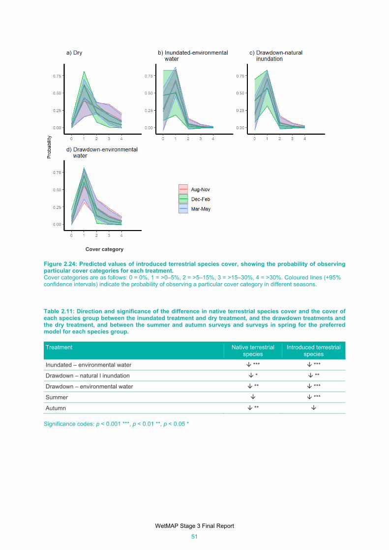
WetMAP Stage 3 Final Report
51
Cover category
Figure 2.24: Predicted values of introduced terrestrial species cover, showing the probability of observing particular cover categories for each treatment. Cover categories are as follows: 0 = 0%, 1 = >0–5%, 2 = >5–15%, 3 = >15–30%, 4 = >30%. Coloured lines (+95% confidence intervals) indicate the probability of observing a particular cover category in different seasons. Table 2.11: Direction and significance of the difference in native terrestrial species cover and the cover of each species group between the inundated treatment and dry treatment, and the drawdown treatments and the dry treatment, and between the summer and autumn surveys and surveys in spring for the preferred model for each species group.
Treatment Native terrestrial species
Introduced terrestrial species
Inundated – environmental water *** ***
Drawdown – natural l inundation * **
Drawdown – environmental water ** ***
Summer ***
Autumn **
Significance codes: p < 0.001 ***, p < 0.01 **, p < 0.05 *
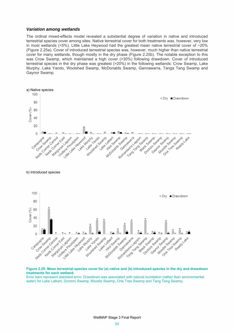
WetMAP Stage 3 Final Report
52
Variation among wetlands
The ordinal mixed-effects model revealed a substantial degree of variation in native and introduced terrestrial species cover among sites. Native terrestrial cover for both treatments was, however, very low in most wetlands (<5%). Little Lake Heywood had the greatest mean native terrestrial cover of ~20% (Figure 2.25a). Cover of introduced terrestrial species was, however, much higher than native terrestrial cover for many wetlands, though mostly in the dry phase (Figure 2.25b). The notable exception to this was Crow Swamp, which maintained a high cover (>30%) following drawdown. Cover of introduced terrestrial species in the dry phase was greatest (>20%) in the following wetlands: Crow Swamp, Lake Murphy, Lake Yando, Woolshed Swamp, McDonalds Swamp, Gannawarra, Tanga Tang Swamp and Gaynor Swamp.
a) Native species
b) Introduced species
Figure 2.25: Mean terrestrial species cover for (a) native and (b) introduced species in the dry and drawdown treatments for each wetland. Error bars represent standard error. Drawdown was associated with natural inundation (rather than environmental water) for Lake Lalbert, Doctors Swamp, Moodie Swamp, One Tree Swamp and Tang Tang Swamp.

WetMAP Stage 3 Final Report
53
Response of lignum to inundation and environmental water KEQ 4: Do environmental water events improve the condition of lignum in wetlands? We found no differences in lignum condition between treatments or between seasons (Appendix 5, Table A5.6, Table 2.12, Figure 2.26). Predicted lignum condition scores were between 8 and 10 (maximum possible score = 12). The estimated between-site (wetland) standard deviation was 4.38, meaning that sites varied substantially in their condition scores relative to treatments (Figure 2.26). In addition, there was a large residual variation (of 4.66 condition points) in the random effects, indicating other factors (such as the antecedent conditions explored in SQ 4 below) could be influencing condition.
Table 2.12: Direction of the difference in the lignum condition score between the inundated treatment and dry treatment, and the drawdown treatments and the dry treatment, and between the summer and autumn surveys and surveys in spring for the preferred model for each species group. Note that none of these effects was significant.
Treatment Lignum condition score
Inundated – environmental water
Drawdown – natural inundation
Drawdown – environmental water
Summer
Autumn
Figure 2.26: Predicted lignum condition scores for the dry and drawdown treatments for wetlands with lignum 0 = poor condition, 12 = excellent condition.
Variation among wetlands
The mean lignum condition score among all wetlands was lowest at Neds Corner Central (mean = 4.1) by a substantial margin (Figure 2.27, Appendix 1, Table A1.2). Lignum at Carapugna was in the best condition. As identified in the linear mixed model (Figure 2.26), there was only a marginal difference in condition scores between the dry and drawdown phase. For most wetlands, the mean was slightly higher in the drawdown phase.
Mea
n Li
gnum
co
nditi
on s
core

WetMAP Stage 3 Final Report
54
Figure 2.27: Mean lignum condition scores from surveys for each wetland with lignum for the dry and drawdown treatments. Note that the absence of drawdown data for the seven wetlands on the right-hand site of the plot, indicate that there was no inundation of lignum in these wetlands. Drawdown was associated with natural inundation (rather than environmental water) for Lake Lalbert and Moodie Swamp.
SQ 4: How does the antecedent water regime affect the condition of lignum in wetlands? Two variables were better fits than the null (intercept-only) model: total days inundated in the prior decade and time since inundation (Appendix 5, Table A5.7, Figure 2.28). However, the model with only total days inundated in the previous decade was the best overall. The lignum condition score was positively related to total days of inundation, increasing from ~7.5 at 0 days inundated to ~11 at over 3000 days inundated. However, this relationship was not particularly strong (R2 = 0.13). It should be noted, however, that the reliability of these predictions at the upper end of inundation is affected by the scarcity of lignum condition data from high antecedent inundation contexts.
Figure 2.28: Model prediction showing relationship between lignum condition and the number of days inundated in the decade prior.
Soil moisture data in the lignum root zone at Lake Murphy
Over the course of the soil moisture monitoring period (December 2018–January 2020), soil moisture was greatest at the surface in the winter months and again (briefly) in early November (Figure 2.29). This was in response to rainfall (110 mm over winter and 20 mm 2–8 November was observed at Kerang Station, 5 km from Lake Murphy). A similar pattern was observed at 15 cm depth, but to a lesser degree, and the soil moisture was slightly less responsive to the rainfall events. At greater depths (>25 cm), moisture was constant over the course of the monitoring period, and relatively high (20–35 mm).
Total days of inundation in prior decade

WetMAP Stage 3 Final Report
55
Figure 2.29: Soil moisture at various depths in the lignum root zone at Lake Murphy.
Response of trees to inundation and environmental water KEQ 5: Do environmental water events lead to growth and flowering of mature wetland tree species?
Tip growth
The tip growth scores of both eucalypt species varied in response to inundation treatment and rainfall. Tip growth scores for River Red Gum were lower in the dry treatment than either of the other two treatments (River Red Gum) and for Black Box they were lower in the dry treatment than the drawdown (environmental water inundation) treatment (Figure 2.30a and 2.30b, Appendix 5, Table A5.8). Note that there were only three trees in the drawdown (natural inundation) treatment for Black Box, and they were therefore removed from the data set before analysis of tip growth and flowering.
In the dry treatment, the probability of observing a tip growth score for River Red Gum of 0 or 1 was ~0.4, and the probability of observing a score of 3 in the dry was ~0 (Figure 2.31a). In comparison, there was a higher probability of observing scores of 2 or 3 during either drawdown treatment. Similarly, for Black Box, the probability of observing a score of 0 was >0.4 during the dry, and the probability of observing a score of 3 was very low (<0.1); in comparison, the probability of observing a score of 2 was ~0.5 during the drawdown (environmental water inundation) phases (Figure 2.31b).
For both species, the probability of observing low scores (0 or 1) was positively related to rainfall in the previous three months (Figure 2.31c and d, Appendix 5, Table A5.8). For River Red Gum, lower scores were more likely when the mean daily temperature in the past three months had been lower (Figure 2.28e).
Flowering
Flowering scores for River Red Gum were highest in the drawdown (natural inundation) treatment than the dry and the drawdown (environmental water inundation) treatment (Figure 2.30c, Figure 2.32a, Appendix 5, Table A5.9). No effects of rainfall or temperature were detected. For Black Box, there was no statistically significant effect of inundation treatment (Figure 2.30d) or temperature (Appendix 5, Table A5.9). However, the probability of lower scores (0 or 1) was positively related to temperature. Conversely, scores of 3 were highest when rainfall in the previous three months was lowest (a probability of 0.6 at 25 mm versus a probability of <0.2 at 150 mm) (Figure 2.32b).

WetMAP Stage 3 Final Report
56
Figure 2.30: Mean scores among wetlands for tip growth in (a) River Red Gum and (b) Black Box, and flowering extent in (c) River Red Gum and (d) Black Box for each inundation treatment. Note that these ignore the hierarchical nature of the data (i.e. all points are being treated as independent, and not nested within wetlands as in the mixed-effects model). Maximum tip growth and flowering score = 3 (abundant) and minimum = 0 (no tip growth or flowering) (refer to Appendix 1, Tables A1.4 and A1.5 for scores and descriptions).
River Red Gum Black Box
Black Box River Red Gum

WetMAP Stage 3 Final Report
57
Figure 2.31: Predictions of the effects of hydrological treatment, rainfall and temperature on tip growth score for River Red Gum and Black Box. In the first two top panels, the lines show the probability of observing a particular condition score as a function of hydrological treatment. In last top panel and bottom two panels, the lines show the probability of observing a particular score as a function of rainfall and temperature respectively. The mean (and 95% confidence intervals) are shown. Maximum tip growth score is 3 (abundant) and minimum = 0 (no tip growth) (refer to Appendix 1, Table A1.4 for scores and descriptions).
Figure 2.32: Predictions of the effects of (a) hydrological treatment for River Red Gum, and (b) rainfall on Black Box flowering. Maximum flowering score is 3 (abundant) and minimum = 0 (no tip flowering) (refer to Appendix 1, Table A1.5 for scores and descriptions).
Tip growth score
Flowering score
Tip growth score
Tip growth score

WetMAP Stage 3 Final Report
58
KEQ 6: Did environmental water support survival of mature trees? Among all wetlands, 589 River Red Gum mature and old mature individuals (13 wetlands) and 941 mature and old mature Black Box individuals (5 wetlands) were recorded from counts within the sampling plots. Over the course of the monitoring, fewer than half of the River Red Gum individuals were inundated (23% from environmental water in three wetlands, and 20% from natural inundation in five wetlands). Of the Black Box, 92% were inundated from environmental water, of which 90% were in one wetland (Little Heywood Lake).
Tree survivorship was high in most wetlands, with mortality observed in only three of 18 wetlands. In two of these (Richardson’s Lagoon and Lake Murphy), the trees were not inundated over the course of the monitoring, though they were located within 100 m of the inundated area. In contrast, trees in the other wetland (Little Lake Heywood) experienced sustained and deep inundation from environmental water (>14 months’ duration, >1.5 m depth) resulting in over 50% mortality of the 825 trees measured there (Table 2.13). The duration and depth of this watering event was unexpected and unintended (see Section 2.4.4).
Table 2.13: Wetlands with tree mortality recorded, with the inundation treatment, time since last inundation event and distance from inundated area.
Wetland Species Mortality Inundation treatment
Richardson’s Lagoon River Red Gum 3% (of 139 trees) Dry >10 years (50–100 m from
inundation)
Lake Murphy Black Box 4% (of 102 trees) Dry ~6 years (<50 m from inundation)
Little Lake Heywood Black Box 51% (of 825 trees) Inundated
Discussion
Understorey vegetation responses to environmental water Response of wetland species richness (KEQ 1) and cover (KEQ 2) to environmental water Environmental water clearly increased both richness and cover of native wetland species, and the response was very similar to that resulting from natural inundation. This was demonstrated by significantly more wetland species and higher cover in the inundated and drawdown treatments than the dry treatment. Species richness in all groups (aquatic, seasonally inundated/immersed and mudflat) was significantly higher in the drawdown treatment (following watering) than the dry treatment. In terms of cover, aquatic and mudflat species were significantly higher in the drawdown treatment than in the dry treatment.
Although, overall, more species and higher cover were observed for the drawdown treatment, in some wetlands both metrics were also high for the dry treatment (e.g. Vinifera, Moodie Swamp, Black Swamp, Gaynor Swamp and One Tree Swamp). Mostly, these were seasonally inundated/immersed species, including Southern Cane-grass (at Moodie Swamp; Figure 2.33), Common Swamp Wallaby-grass (at Black Swamp), Common Spike-sedge (at Vinifera) and Salt Club-sedge (Bolboschoenus caldwellii) and Tangled Lignum (at Reedy Lake). While the above ground biomass of these species can die back, rootstocks of a number of these (Southern Cane-grass, Common Spike-sedge and Salt Club-sedge) survive, and we therefore included these in our species richness and cover observations. Some of these species also experienced natural seasonal dieback due to the onset of either cold or dry conditions.
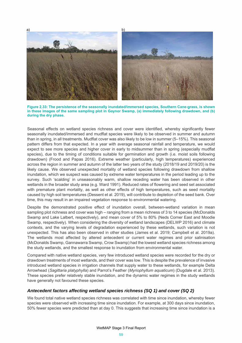
WetMAP Stage 3 Final Report
59
a) b)
Figure 2.33: The persistence of the seasonally inundated/immersed species, Southern Cane-grass, is shown in these images of the same sampling plot in Gaynor Swamp, (a) immediately following drawdown, and (b) during the dry phase.
Seasonal effects on wetland species richness and cover were identified, whereby significantly fewer seasonally inundated/immersed and mudflat species were likely to be observed in summer and autumn than in spring, in all treatments. Mudflat cover was also likely to be low in summer (5–15%). This seasonal pattern differs from that expected. In a year with average seasonal rainfall and temperature, we would expect to see more species and higher cover in early to midsummer than in spring (especially mudflat species), due to the timing of conditions suitable for germination and growth (i.e. moist soils following drawdown) (Frood and Papas 2016). Extreme weather (particularly, high temperatures) experienced across the region in summer and autumn of the latter two years of the study (2018/19 and 2019/20) is the likely cause. We observed unexpected mortality of wetland species following drawdown from shallow inundation, which we suspect was caused by extreme water temperatures in the period leading up to the survey. Such ‘scalding’ in unseasonably warm, shallow receding water has been observed in other wetlands in the broader study area (e.g. Ward 1991). Reduced rates of flowering and seed set associated with premature plant mortality, as well as other effects of high temperatures, such as seed mortality caused by high soil temperatures (Dessent et al. 2019), will contribute to depletion of the seed bank. Over time, this may result in an impaired vegetation response to environmental watering.
Despite the demonstrated positive effect of inundation overall, between-wetland variation in mean sampling plot richness and cover was high – ranging from a mean richness of 3 to 14 species (McDonalds Swamp and Lake Lalbert, respectively), and mean cover of 5% to 80% (Neds Corner East and Moodie Swamp, respectively). When considering the diversity of wetland landscapes (DELWP 2016) and climate contexts, and the varying levels of degradation experienced by these wetlands, such variation is not unexpected. This has also been observed in other studies (James et al. 2019; Campbell et al. 2019a). The wetlands most affected by altered antecedent or current water regimes and prior salinisation (McDonalds Swamp, Gannawarra Swamp, Crow Swamp) had the lowest wetland species richness among the study wetlands, and the smallest response to inundation from environmental water.
Compared with native wetland species, very few introduced wetland species were recorded for the dry or drawdown treatments of most wetlands, and their cover was low. This is despite the prevalence of invasive introduced wetland species in irrigation channels that supply water to these wetlands, for example Delta Arrowhead (Sagittaria platyphylla) and Parrot’s Feather (Myriophyllum aquaticum) (Dugdale et al. 2013). These species prefer relatively stable inundation, and the dynamic water regimes in the study wetlands have generally not favoured these species.
Antecedent factors affecting wetland species richness (SQ 1) and cover (SQ 2)
We found total native wetland species richness was correlated with time since inundation, whereby fewer species were observed with increasing time since inundation. For example, at 300 days since inundation, 50% fewer species were predicted than at day 0. This suggests that increasing time since inundation is a

WetMAP Stage 3 Final Report
60
key factor in reducing the number of wetland species present, as was also observed by Campbell et al. (2019b) and James et al. (2019).
With respect to species groups, we found significant relationships between the richness and cover of aquatic species and the antecedent period of inundation. Such species include Myriophyllum spp., Nardoo (Marsilea drummondii) and River Club-sedge (Schoenoplectus tabernaemontani). The model predicted an additional aquatic species for every 1000 days of inundation in the decade prior, and maximum species richness at permanent inundation. Cover was predicted to increase from <2% with no inundation in the prior decade, to >90% at permanent inundation. Uncertainty increased with time inundated, however, which was likely a reflection of the distribution of data (more than 75% of vegetation plots were inundated for <50% of the prior decade, and none was permanently inundated). Additionally, we know from other studies (Casanova and Brock 2000; Stokes et al. 2010; Raulings et al. 2011; Altenfelder et al. 2016) that permanently inundated wetlands have fewer species than those that dry periodically. Including sites with greater antecedent inundation in future analyses will improve prediction confidence and reduce the uncertain predictions at the upper end of the gradient.
While increases in the total duration of inundation might benefit some aquatic species (Nicol et al. 2003), others (e.g. those that require drawdown periods for recruitment) are likely to be disadvantaged. We found evidence of this, whereby the richness and cover of seasonally inundated/immersed species such as Southern Cane-grass, Common Swamp Wallaby-grass and Common Spike-sedge, and dampland species such as Common Blown-grass (Lachnagrostis filiformis), Clammy Goosefoot (Dysphania pumilio) and Stiff Cup-flower (Pogonolepis muelleriana) decreased as prior inundation increased. This is consistent with our understanding of their intolerance to sustained inundation (Casanova 2011; Frood and Papas 2016). Water regime variability over medium to long time scales (>10 years) is therefore likely to promote a higher overall diversity of wetland species and is an important consideration when managing water regimes for biodiversity outcomes.
With respect to mudflat species such as Pale Knotweed (Persicaria lapathifolia), Common Sneezeweed (Centipeda cunninghamii) and Small Knotweed (Polygonum plebeium) (Figure 2.34), we found an effect of prior inundation frequency on species richness, but not cover. The model predicted higher richness with greater inundation frequency, and a doubling of species as frequency increased from 1 in 10, to 8 in 10 years (noting that we defined an inundation event as inundation of >30 days duration). This relationship has also been observed in seedbank experiments, though these studies operate over much shorter timescales (Casanova and Brock 2000; Altenfelder et al. 2016). While it may appear that high inundation frequency is beneficial for species that germinate on mud, we also recorded a large cover response to inundation of mudflat species such as Southern Liquorice (Glycyrrhiza acanthocarpa) and the endangered Hoary Scurf-pea (Cullen cinereum)3 in a wetland with a very low inundation frequency (Little Lake Heywood with 1 in 20-years flooding). This indicates the presence of an abundant and persistent seedbank, which has been documented in other semi-arid wetlands (Brock et al. 2003; Brock 2011; Nielsen et al. 2018).
A more significant driver of mudflat species response than inundation frequency, and impacting both richness and cover, was the effect of temperature. Fewer species and lower cover were predicted with a higher mean maximum temperature during the three months prior to survey (e.g. sites with a mean maximum temperature of 15°C in the three months prior had 30% predicted cover, in contrast to just 1% at 35°C). This is related to the seasonal influence that we also identified for the relationship between cover of mudflat species in summer and maximum temperature in the three months prior to survey, that is, fewer species and lower cover were predicted in summer and autumn, when extreme temperatures were experienced. We observed evidence of this during our 2018 and 2019 drawdown surveys, with widespread mortality of mudflat species (including Pale Knotweed) occurring before flowering and seed set. This was particularly noticeable in the Mallee sites (especially Neds Corner), where temperatures exceeded 35°C during and 45°C after drawdown (Bureau of Meteorology 2020). Negative impacts of high summer air temperatures have been observed for flood-tolerant species in riparian systems, with reductions in cover likely due to desiccation following unseasonal flooding (Greet et al. 2013). Experiments have also demonstrated that high soil temperatures (in excess of 70°C) can reduce the viability of seeds
3 Classified endangered in Victoria (DEPI 2014, see Appendix 4)
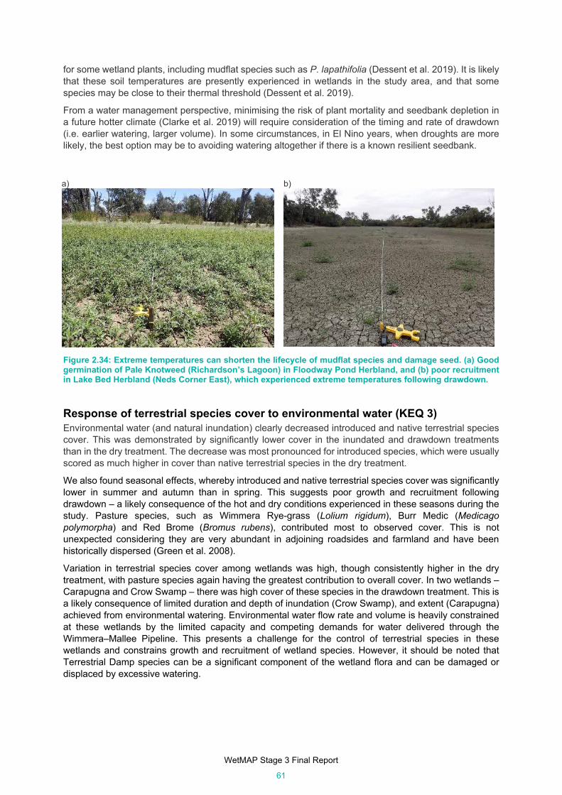
WetMAP Stage 3 Final Report
61
for some wetland plants, including mudflat species such as P. lapathifolia (Dessent et al. 2019). It is likely that these soil temperatures are presently experienced in wetlands in the study area, and that some species may be close to their thermal threshold (Dessent et al. 2019).
From a water management perspective, minimising the risk of plant mortality and seedbank depletion in a future hotter climate (Clarke et al. 2019) will require consideration of the timing and rate of drawdown (i.e. earlier watering, larger volume). In some circumstances, in El Nino years, when droughts are more likely, the best option may be to avoiding watering altogether if there is a known resilient seedbank.
a) b)
Figure 2.34: Extreme temperatures can shorten the lifecycle of mudflat species and damage seed. (a) Good germination of Pale Knotweed (Richardson’s Lagoon) in Floodway Pond Herbland, and (b) poor recruitment in Lake Bed Herbland (Neds Corner East), which experienced extreme temperatures following drawdown.
Response of terrestrial species cover to environmental water (KEQ 3) Environmental water (and natural inundation) clearly decreased introduced and native terrestrial species cover. This was demonstrated by significantly lower cover in the inundated and drawdown treatments than in the dry treatment. The decrease was most pronounced for introduced species, which were usually scored as much higher in cover than native terrestrial species in the dry treatment.
We also found seasonal effects, whereby introduced and native terrestrial species cover was significantly lower in summer and autumn than in spring. This suggests poor growth and recruitment following drawdown – a likely consequence of the hot and dry conditions experienced in these seasons during the study. Pasture species, such as Wimmera Rye-grass (Lolium rigidum), Burr Medic (Medicago polymorpha) and Red Brome (Bromus rubens), contributed most to observed cover. This is not unexpected considering they are very abundant in adjoining roadsides and farmland and have been historically dispersed (Green et al. 2008).
Variation in terrestrial species cover among wetlands was high, though consistently higher in the dry treatment, with pasture species again having the greatest contribution to overall cover. In two wetlands – Carapugna and Crow Swamp – there was high cover of these species in the drawdown treatment. This is a likely consequence of limited duration and depth of inundation (Crow Swamp), and extent (Carapugna) achieved from environmental watering. Environmental water flow rate and volume is heavily constrained at these wetlands by the limited capacity and competing demands for water delivered through the Wimmera–Mallee Pipeline. This presents a challenge for the control of terrestrial species in these wetlands and constrains growth and recruitment of wetland species. However, it should be noted that Terrestrial Damp species can be a significant component of the wetland flora and can be damaged or displaced by excessive watering.

WetMAP Stage 3 Final Report
62
Response of lignum to environmental water (KEQ 4) and antecedent factors (SQ 4)
Environmental watering events did not increase the condition of lignum above the already relatively high levels predicted by our models. This was demonstrated by the lack of any significant differences in condition between the inundation treatments. Notably, predicted and observed condition was relatively high (with low variance) in all treatments and wetlands, with only one exception (Neds Corner Central) – which had the driest antecedent inundation regime of all wetlands, with only two inundation events in the past 15 years.
Results from models that examined the relationships between antecedent hydrology and climate variables and lignum condition identified inundation period in the prior decade as the best predictor of condition, more so than recent inundation event characteristics and weather conditions. This relationship was positive and non-linear, whereby condition was predicted to increase from 8 to 10 (out of a maximum of 12) for between 500 and 2000 days inundation in the prior decade (equivalent to 20–60% of this period inundated), then approach an asymptote at near-permanent inundation. The relationship, however, was not strong, likely because we had very few data in the poor–moderate condition range and no sites that had experienced greater inundation. Including such data in future analyses will improve the likelihood of stronger predictions and also enable an evaluation of the lignum condition outcomes (state-transition models) proposed by Overton et al. (2014). Lignum is a component of a range of vegetation assemblages, with different levels of desired cover in these various contexts. For example, it is ideally only a minor component of Intermittent Swampy Woodland, but the dominant component of Lignum Swampy Woodland.
While not revealed as a significant correlate in our models, the patterning and frequency of inundation is also important in defining lignum condition (Rogers and Ralph 2011; Casanova 2015; Bond et al. 2018; Figure 2.35). We can infer, from the antecedent hydrology of the sites with lignum, that frequency of inundation experienced by the study wetlands has probably maintained it in good condition (i.e. 1–6 events in the prior decade). More broadly, across its distribution, lignum occurs in contexts that typically experience similar regimes (Casanova 2015; Frood and Papas 2016). While dry periods may inhibit optimal growth, its distribution also suggests that plants in poor condition have the ability to respond to favourable environmental conditions after up to 10 years without inundation (Rogers and Ralph 2011; Overton et al. 2014; Casanova 2015). It does this by becoming dormant, but its ability to recover from this state decreases as the duration of dry increases (Freestone et al. 2017).
It is also possible that groundwater can impact on the condition of lignum (Freestone et al. 2017). In one of the study wetlands, where lignum that had not been inundated for 10 years but was still in good condition, we observed abundant soil moisture at root depth (~0.5 m) over the course of 13 months. Notably, this subsurface moisture was as high as that in the top 10 cm of soil immediately following substantial rainfall (~30–50 mm over a two-day period). These reservoirs of subsurface moisture appear to be playing a role in sustaining the plants in this area.
While the condition of plants is an important consideration for the management of lignum, other attributes such as clump size (from the perspective of habitat value) and recruitment success are also important. For example, watering lignum every 1–3 years assists in the greatest clump size, promoting waterbird recruitment (Campbell et al. 2019a), and inundation events of ~20 days’ duration, followed by good soil moisture levels, are required for germination of seed (Higgisson and Dwyer 2018).

WetMAP Stage 3 Final Report
63
a) b)
Figure 2.35: Lignum condition is influenced by antecedent water regime. (a) Lignum in poor condition (shrubs grey/brown, almost entirely senesced) at Neds Corner Central at a location that had experienced very dry antecedent conditions and, contrastingly, (b) lignum in good condition at Hird Swamp, where regular inundation had occurred.
Response of tree tip growth and flowering to inundation and environmental water (KEQ 5)
We found a greater magnitude of tip growth in both River Red Gum and Black Box trees that had been inundated by environmental water, compared with those that had not been inundated (for >9 months). For Black Box trees, this response was observed mainly in trees near the wetland’s edge, which were not subject to the deep, sustained inundation experienced by the remainder of the wetland. Deep inundation resulted in high mortality of trees (see KEQ 6). Moxham et al. (2018) also found greater tip growth in Black Box trees recently inundated, compared with those that had not experienced recent inundation.
As well as the influence of inundation treatment, less tip growth was observed for both species when recent rainfall was higher, and for River Red Gum only when recent maximum temperature was lower. There was, however, a high degree of uncertainty in the modelled responses. This was likely a consequence of the low variation in rainfall among wetlands with trees that had more growth compared with those with less (<50 mm variation over three months) and the ordinal nature of the tip growth data. In contrast to the modelled predictions, River Red Gum and Black Box phenology are reported as having peak leaf production under wet conditions and in summer (Jensen et al. 2007), indicating that more detailed tip growth data captured over a broader rainfall gradient is required in order to validate our model predictions.
Flowering was not greater with either River Red Gum or Black Box trees that were inundated with environmental water (or natural inundation) compared with trees that were not inundated. Indeed, flowering was more abundant in the dry treatment. Many of the trees with a large amount of flowering were last inundated in 2010 from natural floods that occurred during a strong La Nina event. Jensen et al. (2007) note that such antecedent events are an important determinant of the flower crop for both species. Additionally, flushes of flowering of Black Box at dry times could be a bet-hedging strategy – commonly employed in semi-arid flora to enable persistence of populations in harsh climates (Childs et al. 2010).
Survival of mature trees (KEQ 6) The survivorship of mature and old mature River Red Gum trees was very high among wetlands, despite >50% of trees in the wetlands that received environmental water not being inundated (i.e. the water did not reach the areas with trees). Therefore, their survival is likely sustained by rainfall, groundwater and previous inundation events. River Red Gum mortality was observed in only one of our study wetlands (Richardson’s Lagoon), on dry elevated terraces that had not been inundated for ~10 years. Depending on location, the inundation requirements for River Red Gum growth are reported as being 3–7 events in 10 years (Roberts and Marston 2011; Rogers and Ralph 2011; Doody et al. 2015; Casanova 2015). State-and-transition models developed by Overton et al. (2014) indicate that trees in woodland areas on the

WetMAP Stage 3 Final Report
64
Murray River floodplain transition from good to critical condition in 13 years, that is trees in good condition can survive up to 13 years without inundation. We have insufficient data (e.g. groundwater data) to be able to determine whether this mortality is a result of inadequate water availability; however, these studies suggest that it is a likely factor. No mortality was observed at the 11 other River Red Gum wetlands that had higher inundation frequencies.
In contrast, almost all of the Black Box trees assessed were inundated. These, however, were from one wetland (Little Lake Heywood), which had the greatest population of Black Box among the study wetlands. In this wetland, we observed >50% mortality in the sampling plots closer to the centre of the wetland, following an environmental water event that was unintentionally and unexpectedly long (15 months) and deep (>1.5 m in the middle of the wetland). Less water was absorbed into the bed of the wetland and underlying geology than anticipated, which resulted in a larger volume of water persisting in the wetland than expected. While the trees at the edge of the wetland were also inundated, the duration and depth were less (~6 months, <0.5 m), and these trees survived and produced new leaves in response to the inundation (see KEQ 5). Black Box are less tolerant to inundation than River Red Gum (George et al. 2005; Jensen et al. 2007) and more tolerant to dry conditions. Floods of the duration and depth observed at Little Lake Heywood are very rare in these communities (Overton et al. 2014).
A small population of mature Black Box (five trees) on the eastern shore of Lake Murphy also died during the study (they were in good condition at the commencement of the study). This was not likely in response to extreme dry or wet conditions, because these trees were very close to an area inundated from environmental water, and trees on the western shore, at similar elevation, were healthy throughout the study. The cause of this rapid mortality is unknown and requires further investigation. Such rapid changes in the condition of Black Box are unusual, as this species usually responds to flooding and drought over an extended period (Slavich et al. 1999; Roberts et al. 2009; Casanova 2015). For example, an analysis of long-term data sets (Roberts et al. 2009) found that medium-term flood history (5–50 years) is a more important predictor of overall health of Black Box, than recent history (1–5 years) (Overton et al. 2014), and Casanova (2015) suggests that inundation every 10–20 years is required for vigorous growth. River Red Gum, however, responds over shorter time scales (Roberts et al. 2009; Wen et al. 2009).
Because of low inundation frequency, it appears that the low-inundation critical threshold for River Red Gum growth has been crossed in parts of some study wetlands (e.g. woodland surrounding Richardson’s Lagoon) and, conversely, too much inundation (a long and deep event) has exceeded the survival threshold for Black Box at Little Lake Heywood.
Conclusions and future directions Efficacy of Wetland Insights Tool hydrology data The data from tool for the majority of wetlands was very useful for exploring relationships between vegetation dynamics and antecedent hydrology. For some wetlands however, the tool produced spurious data, primarily because of dense tree canopy (Landsat sensors cannot ‘see’ through this), and these data were removed prior to undertaking the analyses (see Section 2.2.4 and Appendix 3). It should also be noted that the temporal and spatial resolution of the data are constrained by the frequency of satellite passes (every 16 days), cloud cover and spatial resolution of the satellite sensors (30 x 30 m). To improve detection of water in the sampling plots, we added a 5-m buffer to our plots to ensure that a Landsat pixel was always located inside the plot, and we used a low inundation extent threshold (15% of the sampling plot) to define an inundation event. Wetland topography can influence water regimes at fine scales (Boon et al. 2008; Raulings et al. 2011) and therefore subsequent, more detailed, investigations of antecedent hydrology should include hydrology data collected and measured at these scales – for example from a combination of depth sensors placed in the wetland, and bathymetric mapping, which can be used to extrapolate depth to other locations in the wetland.
Wetland context and key findings We found that environmental watering in our study wetlands supported the growth of much of the extant wetland vegetation and suppressed terrestrial understorey species, in a very similar way to natural inundation. This is despite the relatively poor condition of some of these wetlands, resulting from modified antecedent water regimes, and degradation from other related impacts (such as siltation from irrigation) (see Figure 2.36). We also observed responses in wetlands that demonstrate how resilient wetland vegetation can be – notably the flush of aquatic and mud herb seedbank species (some rare, such as the

WetMAP Stage 3 Final Report
65
Hoary Scurf-pea in Little Lake Heywood, which had not been previously inundated for over two decades). These species demonstrated an abundant and persistent seedbank at this wetland.
In some wetlands, the degradation of the wetland vegetation communities from the historic legacy effects is severe, particularly where there has been substantial reduction in – and in some wetlands, the total loss of – trees (Black Box and River Red Gum), which were once scattered through many of these wetlands. In these cases, the capacity of environmental water (and restoration of inundation regimes more broadly) to recover or improve wetland vegetation may need to be assisted by additional management actions such as revegetation. Such actions are being implemented in the study area, including planting of aquatic species and River Red Gum in Hird Swamp, McDonalds Swamp and Lake Yando.
Of relevance to longer-term water planning and management was the demonstrated effect of the antecedent water regime on herbaceous understorey vegetation and lignum, and the impact of extreme temperatures on seasonally inundated/immersed and mudflat species. This means there needs to be a strong focus on implementing appropriate water regimes across the longer term and consideration of climate drivers such as El Nino when planning water delivery.
We also found that the responses of understorey species to antecedent inundation do not necessarily reflect relationships observed in controlled experiments (e.g. Casanova and Brock 2000; Altenfelder et al. 2016); for example, we observed high species richness in some wetlands with quite low inundation frequency and duration. It is perhaps unsurprising that observed responses do not follow these reported patterns when we consider that there are uncontrolled factors and interactions that influence wetland vegetation (Figure 2.36). We also note that controlled experiments are limited in their ability to measure responses over the time frames relevant to many species’ persistence (i.e. 5–10 years or more). Therefore, this highlights the importance of collecting observations over longer time frames or through space-for-time substitution monitoring (Picket 1989).
With respect to trees (River Red Gum and Black Box), we observed a mixed response from environmental water. Positive responses in the limited number of trees that were inundated by environmental water were somewhat outweighed by the mortality of trees from ‘overwatering’, that is, exceeding the maximum threshold of tolerance to inundation duration. Future watering should consider the extent and volume of inundation required to reach populations of these wetland trees, and also be mindful of the consequences of prolonged and deep inundation, particularly for Black Box.
Vegetation considerations for water management and future directions Following on from the demonstrated short-term benefits of environmental water to wetland vegetation, we are now well placed to further explore water regime requirements of wetland vegetation species and assemblages. Critical to water management decisions will be an understanding of optimal water regimes, and thresholds (upper and lower) of vegetation to a single event or regime (e.g. duration of an event, frequency of events). Observed mortality of Black Box to inundation of greater than 15 months clearly indicated that a critical upper threshold of survival was exceeded for this species. We commenced an exploration of watering optima or thresholds for other species and species groups; however, this was constrained by the limited hydrological gradient exhibited among the monitoring sites (few sites experienced minimal or maximal antecedent inundation). Asymptotes in the relationships were, however, identified between some species and groups and water regime characteristics (e.g. mudflat species richness reached an asymptote at inundation frequency 7.5 years in 10, and lignum condition at 1500 days of inundation per decade). It is possible that, with additional data, upper thresholds for these responses may be revealed. A future focus on sites that have experienced a broader range of inundation regimes (analogous to space-for-time monitoring; Pickett 1989) will assist with this task.
State-and-transition models (Westoby et al. 1989; Friedel 1991; Lindig-Cisneros et al. 2003), underpinned by an understanding of critical thresholds, provide a framework for managing water regimes for vegetation. Overton et al. (2014) and Bond et al. (2018) have adapted such models for wetland vegetation that predict the response of wetland vegetation species and communities with different initial starting conditions to consecutive years of inundation (defined as a particular combination of flow magnitude, timing, duration and frequency at a particular site; the site-specific flow indicator or SFI – see Figure 2.4). These models incorporate the state dependency of biotic response to inundation (water regime requirements and the myriad of effects from other activities and other processes – see Figures 2.1 and 2.36), thereby representing the influences of both antecedent and current conditions.

WetMAP Stage 3 Final Report
66
Next steps Utilising the aforementioned approaches in WetMAP Stage 4 could involve the following steps:
1. Identify important wetland species, assemblages, and/or vegetation strata from existing vegetation objectives for watered wetlands (in EWMPs) and identify objectives for wetlands that could potentially receive environmental water (both where infrastructure exists and where there is no present water delivery infrastructure). Now that considerable data and observations on most sites that receive environmental water have been collected, a review of the existing objectives by CMAs and wetland ecologists is possible. Review (of the existing objectives) and the setting of new objectives, should be informed by conceptual models that show links between wetland values and the vegetation attributes that support them.
2. Improve model predictions from Stage 3 for the species and assemblages identified in Step 1. This could be assisted by adjusting some aspects of the study design and exploring other options for current and antecedent hydrological data used in the analysis. For example, the following could be addressed: (i) altered timing and frequency of sampling to better capture the rapid response of vegetation following drawdown (particularly the cover of aquatic species), (ii) together with Geoscience Australia, resolve water detection issues at fine scales, and (iii) acquire hydrology data (including depth) at each sampling location (e.g. by using detailed wetland digital elevation models to extrapolate depth data obtained from gauge boards and depth sensors).
3. Based on current understanding of the tolerance limits of vegetation of interest, target biological data collection at sites that span a broader hydrological gradient (i.e. varying inundation histories) to identify critical upper and lower thresholds for vegetation species, assemblages and/or strata (and also other biota – ensuring that the scales relevant for maintenance of processes are considered).
4. Identify possible vegetation condition states and benchmark the ‘best possible condition’ for these species and groups. This action will need to consider the objectives of environmental watering and various climate scenarios (especially that of a drier climate).
5. Identify thresholds for various condition states (e.g. Overton et al. 2014; Bond et al. 2018).
6. Identify the trade-offs among species and water regimes required to maintain and, where possible, improve the condition of vegetation assemblages.
Specific experiments and investigation that could contribute to these steps could include:
Examine seedbank longevity/resilience through a controlled experiment (e.g. Brock 2011) by wetting sediments from wetlands that have had minimal inundation over the prior two decades [informs Steps 4 and 5].
Examine effects of water temperature on germination and growth responses of aquatic species, and the effects of soil temperature on germination and growth responses of mudflat species, through a controlled experiment [informs Steps 4 and 5].
Together with the bird, frog and fish teams, determine vegetation condition states for habitat values provided by vegetation [informs Steps 5 and 6].
Develop hypotheses to test the cause of unexplained Black Box mortality (which could include saline groundwater, for example) [fills a knowledge gap identified in this study and informs Step 5].
Please refer to Chapter 7 for an overview of the suggested next steps for WetMAP Stage 4 that consider all biota.
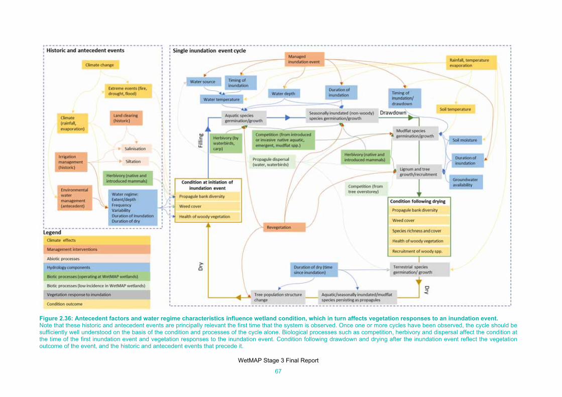
WetMAP Stage 3 Final Report
67
Figure 2.36: Antecedent factors and water regime characteristics influence wetland condition, which in turn affects vegetation responses to an inundation event. Note that these historic and antecedent events are principally relevant the first time that the system is observed. Once one or more cycles have been observed, the cycle should be sufficiently well understood on the basis of the condition and processes of the cycle alone. Biological processes such as competition, herbivory and dispersal affect the condition at the time of the first inundation event and vegetation responses to the inundation event. Condition following drawdown and drying after the inundation event reflect the vegetation outcome of the event, and the historic and antecedent events that precede it.

WetMAP Stage 3 Final Report
68
References Altenfelder, S., Schmitz, M., Poschlod, P., Kollmann, J. and Albrecht, H. (2016). Managing plant species diversity
under fluctuating wetland conditions, the case of temporarily flooded depressions. Wetlands Ecology and Management 24 (6), 597–608.
Barrett, R., Nielsen, D.L. and Croome., R. (2010). Associations between the plant communities of floodplain wetlands, water regime and wetland type. River Research and Applications 26, 866–876.
Bates, D., Mächler, M., Bolker, B. and Walker, S. (2015). Fitting linear mixed-effects models using lme4. Journal of Statistical Software 67, 1–48.
Bennetts, K. and Sim, L. (2016). Gunbower Forest Wetland Exclusion Study, Spring–Summer Report May 2016. Report prepared for the North Central Catchment Management Authority, Melbourne.
Bond N.R., Grigg N., Roberts, J., McGinness, H., Nielsen, D., O’Brien, M., Overton, I., Pollino, C., Reid, J.R.W. and Stratford, D. (2018). Assessment of environmental flow scenarios using state-and-transition models. Freshwater Biology 63 (8), 804–816.
Boon, P.I., Raulings, E., Roache, M. and Morris, K. (2008). Vegetation changes over a four-decade period in Dowd Morass, a brackish-water wetland of the Gippsland Lakes, south-eastern Australia. Proceedings of the Royal Society of Victoria 120, 403–418.
Brock, M.A. (2011). Persistence of seed banks in Australian temporary wetlands. Freshwater Biology 56, 1312–1327.
Brock, M.A. and Casanova, M.T. (1997). Plant life at the edge of wetlands: ecological responses to wetting and drying patterns. In: Klomp, N. and Lunt, I.D. (Eds) Frontiers in Ecology: Building the Links, pp. 181–192. Elsevier Science Ltd, Oxford, UK.
Brock, M.A., Nielsen, D.L., Russell, J., Shiel, R.J., Green, J.D. and Langley, J.D. (2003). Drought and aquatic community resilience: the role of eggs and seeds in sediments of temporary wetlands. Freshwater Biology 48, 1207–1218.
Brooks, M.E, Kristensen, K., van Benthem, K.J, Magnusson, A., Berg, C.W, Nielsen, A., Skaug, H.J., Maechler, M. and Bolker, B.M. (2017). glmmTMB balances speed and flexibility among packages for zero-inflated generalized linear mixed modeling. The R Journal 9, 378–400.
Bureau of Meteorology. (2020). Climate data online. http://www.bom.gov.au/climate/data (accessed July 2020).
Campbell, C.J., Capon, S.J., Gehrig, S.L., James, C.S., Morris, K., Nicol, J.M., Nielsen, D.L. and Thomas R.F. (2019a). Murray‒Darling Basin Environmental Water Knowledge and Research Project – Vegetation Theme Research Report. Report prepared for the Department of the Environment and Energy, Commonwealth Environmental Water Office by La Trobe University, Centre for Freshwater Ecosystems, CFE Publication 226, June 2019.
Campbell, C.J., Capon, S.J., James, C.S., Morris, K., Nicol, J.M., Thomas, R.F., Nielsen, D.L., Gehrig, S.L., Palmer, G.J., Wassens, S., Dyer, F., Southwell, M., Watts, R.J. and Bond, N.R. (2019b). Appendix V 1.1 Conceptualisation Paper: Blue, green and in-between; setting objectives for and evaluating wetland vegetation responses to environmental flows. In: Campbell, C.J., Capon, S.J., Gehrig, S.L., James, C.S., Morris, K., Nicol, J.M., Nielsen, D.L. and Thomas R.F. (2019). Murray‒Darling Basin Environmental Water Knowledge and Research Project – Vegetation Theme Research Report. Report prepared for the Department of the Environment and Energy, Commonwealth Environmental Water Office by La Trobe University, Centre for Freshwater Ecosystems (formerly Murray‒Darling Freshwater Research Centre), CFE Publication 226, June 2019.
Capon, S.J. (2005). Flood variability and spatial variation in plant community composition and structure on a large arid floodplain. Journal of Arid Environments 60, 283–302.
Casanova, M.T. (2011). Using water plant functional groups to investigate environmental water requirements. Freshwater Biology 56, 2637–2652.

WetMAP Stage 3 Final Report
69
Casanova, M.T. (2015). Review of water requirements for key floodplain vegetation for the Northern Basin: literature review and expert knowledge assessment. Report to the Murray‒Darling Basin Authority, Charophyte Services, Lake Bolac, Victoria.
Casanova, M.T. and Brock, M.A. (2000). How do depth, duration and frequency of flooding influence the establishment of wetland plant communities? Plant Ecology 147, 237–250.
Catford, J.A., Downes, B.J., Gippel, C.J. and Vesk, P.A. (2011). Flow regulation reduces native plant cover and facilitates exotic invasion in riparian wetlands. Journal of Applied Ecology 48, 432–442.
Childs, D.Z., Metcalf, C.J.E. and Rees, M. (2010). Evolutionary bet-hedging in the real world: empirical evidence and challenges revealed by plants. Procedings of the Royal Society B 277, 3055–3064
Christensen, R. (2019). Regression Models for Ordinal Data. R Core team. https://cran.r-project.org/web/packages/ordinal/index.html (September 2020).
Clarke, J.M., Grose, M., Thatcher, M., Hernaman, V., Heady, C., Round, V., Rafter, T., Trenham, C. and Wilson, L. (2019). Victorian Climate Projections 2019 Technical Report. CSIRO, Melbourne, Victoria.
Corangamite CMA. (2017). Lower Barwon Wetlands Seasonal Watering Proposal, 2017–18. Corangamite CMA, Colac, Victoria.
Craig, A.E., Walker, K.F. and Boulton, A.J. (1991). Effects of edaphic factors and flood frequency on the abundance of lignum (Muehlenbeckia florulenta Meissner) (Polygonaceae) on the River Murray floodplain, South Australia. Australian Journal of Botany 39, 431–443.
Department of Environment, Land, Water and Planning (DELWP). (2016). The Victorian wetland classification framework. Department of Environment, Land, Water and Planning, East Melbourne, Victoria.
DELWP. (2018). Index of Wetland Condition – assessment of wetland vegetation. Department of Environment, Land, Water and Planning, East Melbourne, Victoria.
DELWP. (2020). Victorian Wetland Inventory (Current). Department of Environment, Land, Water and Planning, East Melbourne, Victoria. https://discover.data.vic.gov.au/dataset/victorian-wetland-inventory-current (accessed July 2020).
Department of Environment and Primary Industries (DEPI). (2014). Advisory List of Rare or Threatened Plants in Victoria – 2014. Department of Environment and Primary Industries, East Melbourne, Victoria.
Department of Sustainability and Environment (DSE). (2005). Index of Wetland Condition. Conceptual framework and selection of measures. Department of Sustainability and Environment, East Melbourne, Victoria.
DSE. (2012). A field guide to Victorian Wetland Ecological Vegetation Classes for the Index of Wetland Condition, 2nd edn. Arthur Rylah Institute for Environmental Research, Heidelberg, Victoria.
Dessent, J., Lawler, S. and Nielsen, D. (2019). The impact of increased temperatures on germination patterns of semi-aquatic plants. Seed Science Research 29, 204–209.
Dobbie, M.F. (2013). Public aesthetic preferences to inform sustainable wetland management in Victoria, Australia. Landscape and Urban Planning 120, 178–189.
Doody, T., Colloff, M.; Davies, M., Koul, V., Benyon, R. and Nagler, P. (2015). Quantifying water requirements of riparian river red gum (Eucalyptus camaldulensis) in the Murray–Darling Basin, Australia – implications for the management of environmental flows. Ecohydrology 8 (8), 1471–1487.
Dugdale, T.M., Hunt, T.D. and Clements, D. (2013). Aquatic weeds in Victoria: where and why are they a problem, and how are they being controlled? Plant Protection Quarterly 28 (2), 35–41.
Dunn, B., Lymburner, L., Newey, V., Hicks, A. and Carey, H. (2019). Developing a tool for wetland characterization using fractional cover, tasseled cap wetness and water observations from space. In: Proceedings of IGARSS 2019–2019 IEEE International Geoscience and Remote Sensing Symposium, Yokohama, Japan, 2019, pp. 6095–6097.

WetMAP Stage 3 Final Report
70
Freestone, F.L., Brown, P., Campbell, C.J., Wood, D.B., Nielson, D.L. and Henderson, M.W. (2017). Return of the lignum dead: resilience of an arid floodplain shrub to drought. Journal of Arid Environments 138, 9–17.
Friedel, M.H. (1991). Range condition assessment and the concept of thresholds: a viewpoint. Journal of Range Management 44, 422–426.
Frood, D. (2007a). Review of information on the ecology of Tangled Lignum. Pathways Bushland and Environment, March 2007. Report to Department of Primary Industries, Kerang.
Frood, D. (2007b). Summary of attributes of the ecology of Tangled Lignum. Pathways Bushland and Environment, December 2007. Report to Department of Primary Industries, Kerang, Victoria.
Frood, D. and Papas, P. (2016). A guide to water regime, salinity ranges and bioregional conservation status of Victorian wetland Ecological Vegetation Classes. Arthur Rylah Institute for Environmental Research Technical Report Series No. 266. Department of Environment, Land, Water and Planning, Heidelberg, Victoria.
George, A.K., Walker, K.F. and Lewis, M.M. (2005). Population status of eucalypt trees on the River Murray floodplain, South Australia. River Research and Applications 21, 271–282.
GHD. (2011). Concept designs for waterway management options, Tang Tang Swamp, September 2011. Report to the North Central Catchment Management Authority, Huntly, Victoria.
GHD. (2017). Reedy Lake Environmental Flow and Monitoring Restoration Project – integrated monitoring report. Report to Corangamite Catchment Management Authority, Colac, Victoria.
Goulburn Broken CMA. (2011a). Black Swamp Environmental Water Management Plan. Goulburn Broken Catchment Management Authority, Shepparton, Victoria.
Goulburn Broken CMA. (2011b). Doctors Swamp Draft Environmental Water Management Plan. Goulburn Broken Catchment Management Authority, Shepparton, Victoria.
Goulburn Broken CMA. (2012a). Gaynor Swamp Environmental Water Management Plan. Goulburn Broken Catchment Management Authority, Shepparton, Victoria.
Goulburn Broken CMA. (2012b). Moodie Swamp Environmental Water Management Plan. Goulburn Broken Catchment Management Authority, Shepparton, Victoria.
Green, A.J., Jenkins, K.M., Bell, D., Morris, P.J. and Kingsford, R.T.I. (2008). The potential role of waterbirds in dispersing invertebrates and plants in arid Australia. Freshwater Biology 53 (2), 380–392.
Greet, J., Cousens, R.D. and Webb, J.A. (2013). Seasonal timing of inundation affects riparian plant growth and flowering: implications for riparian vegetation composition. Plant Ecology 214, 87–101.
Higgisson, W., Briggs, S. and Dyer, F. (2018). Seed germination of tangled lignum (Duma florulenta) and nitre goosefoot (Chenopodium nitrariaceum) under experimental hydrological regimes. Marine and Freshwater Research 69, 1268–1278.
James, C.S., Campbell, C.J., Capon, S., Morris, K., Nicol, J.M., Thomas, R.F., Nielsen, D.L., Gehrig, S.L., Keogh, A. and Thomson, J.R. (2019). Appendix V2.1: Data integration and synthesis component paper: Disentangling flow–vegetation relationships and antecedent legacies to inform environmental flows. In: Campbell, C.J., Capon, S.J., Gehrig, S.L., James, C.S., Morris, K., Nicol, J.M., Nielsen, D.L. and Thomas R.F. (2019). Murray‒Darling Basin Environmental Water Knowledge and Research Project — Vegetation Theme Research Report. Report prepared for the Department of the Environment and Energy, Commonwealth Environmental Water Office by La Trobe University, Centre for Freshwater Ecosystems (formerly Murray‒Darling Freshwater Research Centre), CFE Publication 226, June 2019.
Jansen, A. and Robertson, A.I. (2001). Relationship between livestock management and the ecological condition of riparian habitats along an Australian floodplain river. Journal of Applied Ecology 38, 63–75.

WetMAP Stage 3 Final Report
71
Jensen, E.J., Walker, F.K. and Paton D.C. (2007). Using phenology of eucalypts to determine environmental watering regimes for the River Murray floodplain, South Australia. In: Proceedings of the 5th Australian Stream Management Conference. Australian rivers: making a difference. Charles Sturt University, Thurgoona, New South Wales.
Lindig-Cisneros, R., Desmond, J., Boyer, K.E. and Zedler, J.B. (2003). Wetland restoration thresholds: can a degradation transition be reversed with increased effort? Ecological Applications 13, 193–205.
Mallee CMA. (2012). Margooya Lagoon Floodplain Management Unit Environmental Water Management Plan. Mallee Catchment Management Authority, Mildura Victoria.
Mallee CMA. (2015). Nyah and Vinifera Environmental Water Management Plan. Mallee Catchment Management Authority, Mildura, Victoria.
Morris, K. (2012). Wetland connectivity: understanding the dispersal of organisms that occur in Victoria’s wetlands. Arthur Rylah Institute for Environmental Research Technical Report Series No. 225. Department of Sustainability and Environment, Heidelberg, Victoria.
Moxham, C., Duncan, M. and Moloney, P. (2018). Tree health and regeneration response of Black Box (Eucalyptus largiflorens) to recent flooding. Ecological Management and Restoration 19, 58–65.
Nicol, J.M., Ganf, G.G. and Pelton, G.A. (2003). Seed banks of a southern Australian wetland: the influence of water regime on the final floristic composition. Plant Ecology 168, 191–205.
Nicol, J., Muston, S., D’Santos, P., McCarthy, B. and Zukowski, S. (2007). Impact of sheep grazing on the soil seed bank of a managed ephemeral wetland: implications for management. Australian Journal of Botany 55, 103–109.
Nielsen, D.L., Campbell, C., Rees, G.N., Durant, R., Littler, R and Petrie, P. (2018). Seed bank dynamics in wetland complexes associated with a lowland river. Aquatic Sciences 80, 23. https://doi.org/10.1007/s00027-018-0574-3
Nielsen, D.L., Podnar, K., Watts, R.J. and Wilson, A.L. (2013). Empirical evidence linking increased hydrologic stability with decreased biotic diversity within wetlands. Hydrobiologia 708, 81–96.
North Central CMA. (2014a). Hird Swamp Environmental Water Management Plan. North Central Catchment Mangaement Authority, Huntly, Victoria.
North Central CMA. (2014b). Richardson’s Lagoon Environmental Water Management Plan. North Central Catchment Management Authority, Huntly, Victoria
North Central CMA. (2015a). Lake Murphy Environmental Water Management Plan. North Central Catchment Management Authority, Huntly, Victoria.
North Central CMA. (2015b). McDonalds Swamp Environmental Water Management Plan. North Central Catchment Management Authority, Huntly, Victoria.
North Central CMA. (2016). Lake Yando Environmental Water Management Plan. North Central Catchment Management Authority, Huntly, Victoria.
Overton, I.C., Pollino, C.A., Roberts, J., Reid, J.R.W., Bond, N.R., Mcginness, H.M., Gawne, B., Stratford, D., Merrin, L., Barma, D., Cuddy, S.M., Nielsen, D.L., Smith, T., Henderson, B.L., Baldwin, D.S., Chiu, G.S. and Doody, T.M. (2014). Development of the Murray–Darling Basin Plan SDL Adjustment Ecological Elements Method. Report prepared by CSIRO for the Murray–Darling Basin Authority, Canberra, Australian Capital Territory.
Papas, P. and Moloney P. (2012). Victoria’s wetlands 2009–2011: statewide assessments and condition modelling. Arthur Rylah Institute for Environmental Research Technical Report Series No. 229. Department of Sustainability and Environment, Heidelberg, Victoria.

WetMAP Stage 3 Final Report
72
Papas, P., Stamation, K. and Downe, J. (2018). WetMAP Vegetation Theme Annual Report 2018. Arthur Rylah Institute for Environmental Research, Department of Environment, Land, Water and Planning, Heidelberg, Victoria.
Pickett, S.T.A. (1989). Space-for-time substitution as an alternative to long-term studies. In: Likens G.E. (Ed.) Long-Term Studies in Ecology. Springer, New York City, New York.
R Core Team. (2020). R: A language and environment for statistical computing. R Foundation for Statistical Computing, Vienna, Austria. http://www.R-project.org/ (accessed June 2020).
Raulings, E.J., Morris, K., Roache, M.C. and Boon, P.I. (2010). The importance of water regimes operating at small spatial scales for the diversity and structure of wetland vegetation. Freshwater Biology 55, 701–715.
Raulings, E.J., Morris, K., Roache, M.C. and Boon, P.I. (2011). Is hydrological manipulation an effective management tool for rehabilitating chronically flooded, brackish-water wetlands? Freshwater Biology 56, 2347–2369.
Roberts, J., Casanova, M.T., Morris, K. and Papas, P. (2017). Vegetation recovery in inland wetlands: an Australian perspective. Arthur Rylah Institute for Environmental Research Technical Report Series No. 270. Department of Environment, Land, Water and Planning, Heidelberg, Victoria.
Roberts, J., Chan, C., Henderson, B. and Overton, I. (2009). Floodplain trees. In: Overton, I.C., Colloff, M.J., Doody, T.M., Henderson, B. and Cuddy, S.M. (Eds) Ecological Outcomes of Flow Regimes in the Murray–Darling Basin. Report prepared for the National Water Commission by CSIRO Water for a Healthy Country Flagship. CSIRO, Canberra, Australian Capital Territory.
Roberts, J. and Marston, F. (2011). Water regime for wetland and floodplain plants: a source book for the Murray–Darling Basin. National Water Commission, Canberra, Australian Capital Territory.
Rogers, K. and Ralph, T. (Eds) (2011). Floodplain wetland biota in the Murray–Darling Basin: water and habitat requirements. CSIRO Publishing, Melbourne, Victoria.
Slavich, P.G., Walker, G.R., Jolly, I.D., Hatton, T.J. and Dawes, W.R. (1999). Dynamics of Eucalyptus largiflorens growth and water use in response to modified watertable and flooding regimes on a saline floodplain. Agricultural Water Management 39, 245–264.
Souter, N., Cunningham, S., Little, S., Wallace, T., McCarthy, B., Henderson, M. and Bennetts, K. (2012). Ground-Based Survey Methods for The Living Murray Assessment of Condition of River Red Gum and Black Box Populations. Murray-Darling Basin Authority, Australian Capital Territory.
Stokes, K., Ward, K. and Colloff, M. (2010). Alterations in flood frequency increase exotic and native species richness of understorey vegetation in a temperate floodplain eucalypt forest. Plant Ecology 211, 219–233.
Vivian, L.M., Godfree, R.C., Colloff, M.J., Mayence, C.E. and Marshall, D.J. (2014). Wetland plant growth under contrasting water regimes associated with river regulation and drought: implications for environmental water management. Plant Ecology 215, 997–1011.
Vivian, L.M., Ward, K.A., Marshall, D.J. and Godfree, R.C. (2015). Pseudoraphis spinescens (Poaceae) grasslands at Barmah Forest, Victoria, Australia: current distribution and implications for floodplain conservation. Australian Journal of Botany 63, 526–540.
Ward, K.A. (1991). Investigation of the flood requirements of the Moira grass plains in Barmah Forest, Victoria. Department of Conservation and Environment, Benalla, Victoria.
Webb, J.A., Wallis, E.M. and Stewardson M.J. (2012). A systematic review of published evidence linking wetland plants to water regime components. Aquatic Botany 103, 1–14.
Weiss, J. and Dugdale, T. (2017). Knowledge document of the impact of priority wetland weeds: Part 2 – Impacts of priority wetland weeds. Report prepared for Department of Environment, Land, Water and Planning (DELWP) Water and Catchments Group by Agriculture Victoria.

WetMAP Stage 3 Final Report
73
Wen, L., Ling, J., Saintilan, N. and Rogers, K. (2009). An investigation of the hydrological requirements of River Red Gum (Eucalyptus camaldulensis) Forest, using classification and regression tree modelling. Ecohydrology 2, 143–55.
Westoby, M., Walker, B. and Noy-Meir, I. (1989). Opportunistic management for rangelands not at equilibrium. Journal of Range Management 42, 266–274.
Wimmera CMA. (2016). Environmental Water Management Plan – Wimmera Mallee Pipeline Wetlands – Wimmera CMA Region. Wimmera Catchment Management Authority, Horsham, Victoria.
Wood, S. and Scheipl, F. (2020). Generalized Additive Mixed Models using 'mgcv' and 'lme4'. R Core Team. https://cran.r-project.org/web/packages/gamm4/gamm4.pdf (September 2020).

WetMAP Stage 3 Final Report
74
3 Frog theme
Introduction
A mass extinction of frogs across the globe is under way (e.g. Alroy 2015; Hirschfeld et al. 2016; Ceballos et al. 2017; O’Hanlon et al. 2018; Grant et al. 2020; Green et al. 2020). Australia is no exception, with reports of frog declines and extinctions increasing in many regions over the last two decades (e.g. Fordham et al. 2016; Potvin et al. 2017; Gillespie et al. 2018; Hunter et al. 2018; Lemckert and Mahony 2018; Ocock and Wassens 2018; Gillespie et al. 2020). While a range of known and putative threats are contributing to these declines, one key process is change to hydrological regimes. For example, the water regime of many Victorian wetlands has been heavily modified over the past 200 years, with changes to the frequency, duration and timing of flooding causing declines in wetland condition.
Altered hydrological regimes are an important threat to frogs because all species are dependent on water for reproduction and survival. Frogs have a biphasic life cycle characterised by eggs being laid in water; typically, both egg and larval development occur in aquatic habitats (although eggs of some species instead develop terrestrially; Anstis 2017; Cogger 2018). One notable feature of the Australian frog fauna is its lack of dependence on permanent bodies of fresh water, and — except for those few genera that lay eggs out of water — its tendency to breed in ephemeral waterbodies (Tyler 1994).
Environmental water is being used to re-establish more natural water regimes and to improve the ‘health’ of wetlands. Hydrology is a key component of wetland health, and frogs can be useful indicators of health because many species respond to changes in hydrology (Wassens et al. 2017). It is critical that the provision of environmental water to benefit the persistence of frogs should accommodate the species’ key needs for timing, duration and frequency so that water requirements for breeding are met (Wassens 2011). In addition, appropriate water delivery must meet other requirements, such as provision of suitable refuges to which frogs can retreat during the day to escape predation or move to during periods of drought.
Key drivers of frog occurrence
Key drivers of frog occurrence operate at both local (wetland) and landscape scales (Figure 3.1). At the local scale, hydrological conditions and other environmental factors (e.g. structural vegetation, water quality) can be used to predict site occupancy (e.g. Wassens et al. 2010). Frogs in the Murray–Darling Basin depend variously on local rainfall or flood pulses (Wassens 2011; Bino et al. 2018). For frogs that are dependent on flood pulses (synonymous with environmental watering in the current study), successful recruitment occurs only when the breeding window, typically spring and summer, and the flood pulse coincide (Wassens 2011). In addition, frog densities respond to other environmental changes in wetlands, such as habitat alteration resulting from grazing by domestic livestock or from the introduction of exotic fish (Jansen and Healey 2003).
Biological and life-history factors, such as lags between calling and spawning, variability in tadpole development times (which can range from several weeks to 12 months, depending on species and environmental conditions) and the predilection for newly metamorphosed individuals to remain close to the natal site while gaining body condition, mean that hydroperiod is an important determinant of frog occurrence (e.g. Wassens 2011; Hamer et al. 2016; Júnior and Rocha 2017; Howell et al. 2020). Hence, recurring reductions in hydroperiod will exclude those species with longer development periods. Conversely, longer hydroperiods can lead to higher predator densities and reduced vegetation complexity, also recognised influences on frog occurrence (Wassens 2010).
While wetland hydroperiod is an important influence, other wetland water characteristics are also likely to influence frog occurrence, including water depth (Queiroz et al. 2015) and water quality, the latter expressed by the degree of salinity (conductivity), pH, turbidity (Simpkins et al. 2014) and contamination (Strong et al. 2017; Sievers et al. 2019), all of which have identifiable impacts on frog larval stages. Habitat structural heterogeneity is important for all frog life stages (e.g. Júnior and Rocha 2017; Marques and Nomura 2018). The composition of any frog assemblage is affected by key habitat components of both the aquatic and proximate terrestrial environments, including riparian or aquatic vegetation, ground cover in adjacent terrestrial environments, and even waterbody size (Healey et al. 1997; McGinness et al. 2014; Villaseñor et al. 2017; Fardell et al. 2018; Pulsford et al. 2019).

WetMAP Stage 3 Final Report
75
To illustrate, froglets (Crinia spp.) prefer areas containing diverse aquatic vegetation, including submerged grasses, whereas Peron’s Tree Frog (Litoria peronii) is associated with arboreal shelter sites provided by standing timber (Wassens 2010, 2011). When wetlands are partly or completely dry, the availability of microhabitats provided by vegetation, coarse woody debris, and soil cracks, support the persistence of frog populations (Amos 2017).
Frogs (including larvae) are important trophic components of freshwater environments, being taken as prey by an assortment of vertebrate and invertebrate predators and in turn preying on select fauna, mostly insects. Predation is known to be a key influence on the structuring of tadpole assemblages, with vertebrate predators (e.g. fish) being important in permanent habitats, but invertebrate predators (e.g. immature Odonata) being the most important in temporary ones (Lowe et al. 2015; Júnior and Rocha 2017). Introduced fish, particularly Mosquitofish (Gambusia spp.), are voracious consumers of tadpoles in Australia (e.g. Hunter et al. 2011; Hamer and Parris 2013; Ocock and Wassens 2018). Other biotic interactions, such as competition and the presence of pathogens, also influence frog occurrence, the latter conspicuously exemplified by chytridiomycosis (from the amphibian fungus Batrachochytrium dendrobatidis), a key global threat to frog persistence (Bellard et al. 2016; Lips 2016; Kolby 2018). The impacts of chytridiomycosis are heavily modified by habitat, including its thermal and chemical aspects, as well as by the presence or absence of tolerant hosts of chytrid (e.g. Heard et al. 2014; Stockwell et al. 2015; Ruggeri et al. 2018). It is hypothesised that those processes could be modified by the provision of environmental water in positive or negative ways, but data on this are lacking.
While local-scale environmental factors affect frog occurrence, it is also important to recognise that many frogs exist within metapopulations (Heard et al. 2012; Hale et al. 2013; Heard et al. 2015b), which are spatially segregated local populations connected by dispersal (Levins 1969, 1970). The distribution of wetlands in northern Victoria is naturally discrete, but this spatial fragmentation has been exacerbated by land clearance, and these characteristics of the landscape have affected the distribution of frogs (Hazell 2003; Cushman 2006; Hale et al. 2013). Physiographic elements are known to influence the capacity of frogs to occupy or move around landscapes prone to variable water regime. These elements include topography (Westgate et al. 2012), number of neighbouring, occupied wetlands (Hamer and Mahony 2010; Scherer et al. 2012), and the area between wetlands that they must move through (i.e. the matrix) (Quesnelle et al. 2015). Landscape connectivity and resistance are important for dispersal and gene flow, which depend on the life-history traits and movement capacity of individual frog species (Richardson 2012; Ishiyama et al. 2014; Watts et al. 2015). Functional connectivity (sensu Auffret et al. 2015) will assume greater importance as the climate changes to a regime of lower rainfall and, very likely, increased habitat fragmentation.
Responses to environmental water
Water is a key factor driving frog occurrence. River regulation and the requirement of water for consumption have reduced aquatic habitat in the Murray–Darling Basin (the Basin), including in northern Victoria, and mitigating these hydrological impacts is a primary focus of water management in this region. Frog monitoring is a key element of major projects within the Basin, such as the Commonwealth government’s The Living Murray program (https://www.mdba.gov.au/publications/brochure/living-murray-program) and the FLOW-MER program (https://flow-mer.org.au/). Like WetMAP, these programs collect data to inform and improve management, leading to the maintenance or improvement of waterway health.
The responses of frogs to environmental watering are expected to vary by species and type of wetland, and are contingent on key elements of the watering regime (notably timing, duration, extent, frequency) (Figure 3.2). If environmental watering is to be implemented over a suitable hydroperiod to benefit the total frog assemblage (or targeted taxa), it should provide variety in water depth, vegetation and structure so as to meet the habitat, life history and movement needs of all (or targeted) taxa. This will ultimately increase the availability of suitable habitat for refuge, feeding and breeding, and will increase functional connectivity. More complex habitats are more likely to foster a higher diversity of species, because more species needs can be met in the same place. Conversely, the provision of water may result in additional threats through increased levels of predation or disease, such as chytridiomycosis. Studies in the USA have found affiliation with ephemeral aquatic habitat and breadth of habitat to be strong predictors of vulnerability to and intensity of chytrid infection (Gervasi et al. 2017).
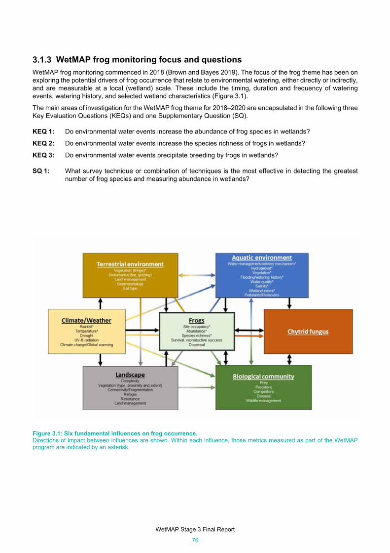
WetMAP Stage 3 Final Report
76
WetMAP frog monitoring focus and questions
WetMAP frog monitoring commenced in 2018 (Brown and Bayes 2019). The focus of the frog theme has been on exploring the potential drivers of frog occurrence that relate to environmental watering, either directly or indirectly, and are measurable at a local (wetland) scale. These include the timing, duration and frequency of watering events, watering history, and selected wetland characteristics (Figure 3.1).
The main areas of investigation for the WetMAP frog theme for 2018–2020 are encapsulated in the following three Key Evaluation Questions (KEQs) and one Supplementary Question (SQ).
KEQ 1: Do environmental water events increase the abundance of frog species in wetlands?
KEQ 2: Do environmental water events increase the species richness of frogs in wetlands?
KEQ 3: Do environmental water events precipitate breeding by frogs in wetlands?
SQ 1: What survey technique or combination of techniques is the most effective in detecting the greatest number of frog species and measuring abundance in wetlands?
Figure 3.1: Six fundamental influences on frog occurrence. Directions of impact between influences are shown. Within each influence, those metrics measured as part of the WetMAP program are indicated by an asterisk.

WetMAP Stage 3 Final Report
77
Figure 3.2: Conceptual model for the response of frogs to environmental water management in wetlands of northern Victoria. Designated links are shown between water delivery (blue), landscape context (red) and biotic components (green).
We acknowledge that KEQs 1–3 are basic questions with respect to the response of frogs to environmental watering in wetlands. However, answering these questions is important because of the need to provide clear evidence of the effects of environmental water delivery in Victorian wetlands. We anticipate that the next stage of WetMAP will develop the focus of examining the relationship between frog responses and aspects of the hydrological regime (as well as individual events) that are linked to their different habitat requirements. The focus of this stage is on answering the four questions above but, with this future focus in mind, we also provide preliminary evidence to start evaluating several longer-term KEQs and SQs, as listed below.
KEQ 4: To what extent does the environmental water regime in wetlands affect the abundance of all resident frog species?
KEQ 5: To what extent does the environmental water regime in wetlands affect the species richness of frogs?
KEQ 6: To what extent does the environmental water regime in wetlands affect breeding by frogs?
SQ 2: Is the composition of frog assemblages related to the timing, frequency and/or duration of environmental watering, or the legacies of water regime history? If so, to what extent do these flow characteristics increase or decrease frog species richness and abundance?
SQ 2a: Is the effect of an environmental water event on richness and abundance of frog species dependent on the hydrological history prior to the watering and over what antecedent period?
SQ 2b: Is the effect of an environmental water event on richness and abundance of frog species dependent on the timing, duration and/or frequency of the watering?
SQ 3: Is the effect of an environmental water event on richness and abundance of frog species dependent on water quality and/or habitat structure?
SQ 4: Is the effect of an environmental water event on richness and abundance of frog species dependent on landscape complexity (especially habitat connectivity and the existence of proximate frog refuges)?

WetMAP Stage 3 Final Report
78
Hypotheses Frog responses to hydrological regimes With these KEQs and SQs in mind, and to illustrate the likely general responses of frogs to environmental watering, in Figures 3.3–3.5 we present the hypothesised effects on frog species richness of the frequency and duration of inundation, and the modulating effects of habitat quality and landscape context, and briefly describe the expected responses below. Other response variables (e.g. overall abundance, and abundance for select species) are likely to approximate the same general trajectories and are included in the formal analyses. It is important to note that we present these response curves as initial predictions that will be tested and refined where necessary as WetMAP progresses.
A positive relationship may exist between frog species richness and frequency of wetland inundation, with seasonally inundated wetlands having the most species due to greater diversity of vegetation and structure (Figure 3.3) (McGinness et al. 2014). However, we expect that there may be a decrease in the number of species at permanent wetlands, where vegetation diversity may be reduced and predator densities (e.g. fish) are likely to be higher. We also predict that the magnitude of the response in species richness will depend on the availability of colonisers from nearby source populations (with an increased magnitude of response and thus greater species richness at wetlands with many potential source populations) and on the season of inundation.
Wetlands subject to seasonal inundation will likely support different numbers of frog species, depending on the duration (hydroperiod) and timing (season) of the inundation (Figure 3.4). To illustrate, tree frogs (Litoria spp.) typically require longer hydroperiods than Crinia species (>6 months cf. 6–12 weeks) for spawning and tadpole development to metamorphosis, although the latter are more able to breed across multiple seasons (Wassens 2011). We expect more frogs to be observed during spring–summer watering than during autumn–winter watering, based on known breeding phenologies.
The effects of the watering regime will also be influenced by the quality of habitat (e.g. availability of breeding, shelter or feeding sites, plus food resources) and the status of source populations (e.g. number and proximity) (Figure 3.5). We have predicted the response in frog species richness and abundance to various types of water regimes, and the influence of habitat quality and status of source populations on that response, acknowledging that these responses will vary between species (e.g. in relation to timing, frequency and hydroperiod). We anticipate that species richness and abundance will be highest at wetlands with suitable water regimes, high quality aquatic habitat and many or close source populations.
Efficacy of frog monitoring techniques Two survey techniques were used: standardised audiovisual surveys and the use of programmable AudioMoth acoustic loggers to record calling frogs.
AudioMoth loggers are a promising tool for environmental monitoring (Hill et al. 2018), but their use is still in its infancy, presenting a number of challenges, such as the limited availability of reference call libraries and open-source tools for processing recordings, as well as a lack of clarity around the accuracy, transferability, and limitations of analytical methods (Gibb et al. 2019). While acoustic loggers have been used to monitor faunal responses to environmental flows (e.g. Linke and Deretic 2020), many of these challenges remain. Over the past 2 years, we have been working to develop and refine acoustic monitoring (AudioMoth), with the hope that this will eventually be a more useful biomonitoring tool. We summarise our findings in this report, highlight some of the challenges with this technique, and outline the next steps for further developing this tool. We present summaries of performances of call recognisers (computer models of taxa-specific frog calls assembled from ‘training data’, i.e. recordings of frog vocalisations) used to identify frog species from calls collected by AudioMoth units, and discuss the advantages that AudioMoth units may provide in detecting additional species.

WetMAP Stage 3 Final Report
79
Figure 3.3: Conceptual models predicting the general response of frog richness to frequency of inundation, and how the number of source populations might modify this response. Frequency of inundation categories from DELWP (2016).
Figure 3.4: Conceptual models predicting the general response of frog richness to duration of inundation, and how the timing of watering might modify this response.
Figure 3.5: Conceptual models predicting the general response of frog richness to water regime and how these relationships might be modified by habitat quality within the wetland, and landscape context (number of and distance to source populations).
WetMAP Stage 3 Final Report
80
Methods
Study wetlands In total, 30 wetlands were monitored during 2018–2020 (Table 3.1). These wetlands were located in the southern portion of the Murray–Darling Basin, within the Goulburn Broken, North Central, Mallee and Wimmera Catchment Management Authority (CMA) regions of northern Victoria. These wetlands represented:
1. a selection of wetlands that receive an environmental water allocation
2. wetlands along a water regime gradient, from those characterised by ephemerality to those holding permanent water
3. wetlands from five different bioregions of northern Victoria (Murray Scroll Belt, Murray Fans, Victorian Riverina, Wimmera, Central Victorian Uplands)
4. wetlands of varying size and landscape context (e.g. isolated vs connected).
The approach to wetland selection varied across the study period. Seventeen wetlands were surveyed in spring–summer 2018–2019, and these represented either intermittent wetlands that were watered at the time of the surveys in spring 2018 or permanently inundated wetlands that may receive environmental water top-ups (Table 3.1) (Brown and Bayes 2019). Twenty-eight wetlands were sampled during 2019–2020, with an increased number to incorporate a larger range of hydrological regimes. The 28 wetlands represented intermittent wetlands that were watered during spring 2019 (either through environmental water allocations or naturally), intermittent wetlands that had retained water from the previous watering, permanently inundated wetlands, and previously watered intermittent wetlands that were dry throughout 2019–2020. These latter wetlands were considered control (‘dry’) wetlands and were used as the test locations for confirming the absence of frogs at dry wetlands (Table 3.1).
Overall, the study wetlands spanned a hydrology gradient from ephemeral wetlands to seasonal wetlands, through to wetlands with permanent or near-permanent hydroperiods. This range was important for identifying the water regime requirements for frog species and assemblages, and for demonstrating the responses of frogs (and other biota) to environmental watering.
Survey area
Monitoring transects were employed as the sampling unit at each wetland in order to ensure a standardised, repeatable approach to frog surveys and habitat assessment. Multiple transects were established at each study wetland, the number being determined by the size of the wetland, the requirements for at least 300 m between transects to avoid double counting of frogs, and ensuring all prevailing vegetation communities were represented (Figure 3.6, Table 3.1). Each transect was 50 m long and positioned so that the midline followed the water’s edge; the locations of the areas relative to the midline varied according to the type of data collected (Figure 3.7). The locations of the start and end points of each transect were recorded by GPS.
Frog survey techniques Two frog sampling methods were used in this study: (i) audiovisual surveys for adult frogs, and (ii) acoustic monitoring using AudioMoth loggers to record calls. These survey techniques are complementary (Wassens et al. 2017) and are designed and timed to best capture frog activity. Taxonomy followed Cogger (2018).

WetMAP Stage 3 Final Report
81
Table 3.1: WetMAP Frog monitoring locations and number of transects for each survey technique for each survey period (2018–2019 and 2019–2020). A total of 17 wetlands were sampled in the first year, and 28 in the second year.
Wetland Wetland
code CMA
2018–2019 2019–2020
Wetland status*
Audiovisual survey
AudioMoth survey
Wetland status*
Audiovisual survey
AudioMoth survey
Black Swamp BLSW GB 1 3 2 4 2 2
Doctors Swamp DOSW GB 2 2
Gaynor Swamp GASW GB 1 5 5 4 2
Horseshoe Lagoon (Trawool)
DOSW GB 1 2 2
Kanyapella Basin KABA GB 2 3
Kinnairds Wetland East
KIWE GB 2 2 2 5 2 2
Kinnairds Wetland West
KIWW GB 1 3 3 2 2
Loch Garry LOGA GB 2 2 2
Moodie Swamp MOSW GB 2 2 2
Reedy Swamp (Shepparton)
RESW GB 1 3 3
Tahbilk Lagoon TALA GB 5 4 4
Cowanna Billabong
COBI Mall 2 4 4 5 4 4
Ducksfoot Lagoon DULA Mall 1 2 2 1 2 2
Kings Billabong KIBI Mall 2 5 5 5 5 5
Neds Corner Central
NECC Mall 1 2 2
Neds Corner East NECE Mall 1 3 3
Neds Corner Woolshed
NECW Mall 1 4 4
Nyah Floodplain NYFL Mall 1 4 4 4 4
Wallpolla Horseshoe Lagoon
WAHO Mall 2 4 4 5 4 4
Johnson Swamp JOSW NC 1 4 4
Lake Bael Bael LABA NC 6 4 4
Lake Murphy LAMU NC 1 3 3 3 3 3
Little Lake Meran LLME NC 1 3 3 3 3 3
McDonalds Swamp
McSW NC 1 3 3 2 2
Richardson's Lagoon
RILA NC 1 5 5 4 2 2
Wirra-Lo Brolga Swamp
WILO_BS NC 1 3 1
Wirra-Lo Duck Creek
WILO_DC NC 1 1 1
Wirra-Lo Lignum Swamp North
WILO_LS NC 1 2 2 3 2
Carapugna CARA Wimm 1 3 3 1 2 2
Crow Swamp CRSW Wimm 1 2 2
Numbers of transects used for audiovisual surveys and AudioMoth surveys are provided. CMA codes: GB = Goulburn Broken, Mall = Mallee, NC = North Central, Wimm = Wimmera For legend for wetland status, see over page.

WetMAP Stage 3 Final Report
82
Table 3.1 notes continued…
* 2018–2019 wetland status Group 1: Spring-watered intermittent wetlands Group 2: Permanently inundated wetlands that may receive environmental water top-ups
2019–2020 wetland status Group 1: Intermittent wetlands that received environmental water in spring Group 2: Intermittent wetlands that received environmental water in autumn (dry in spring, time of survey) Group 3: Intermittent wetlands that received environmental water, which contained water in spring but were not
watered in 2019–2020 Group 4: Previously watered intermittent wetlands that were dry throughout 2019–2020 Group 5: Permanently inundated wetlands that may receive environmental water top-ups Group 6: Naturally watered wetlands (received water from rainfall in spring 2019, dry beforehand)
Adult frog audiovisual surveys
Nocturnal audiovisual surveys for adult frogs were conducted at each monitoring transect – between two and five (mostly five) per wetland – during each visit, depending on prevailing habitat types, wetlandsize and access. Surveys were conducted in spring–summer and consisted of identifying frogs from their calls or by observation during searches with torches. Audiovisual surveys were modified from protocols used in other studies (e.g. Brown et al. 2007; Wassens et al. 2013; Anstis 2017; Wassens et al. 2017); each was conducted by experienced observers, commenced no sooner than 30 minutes after dark and comprised a 5-minute listening period at the approximate midpoint of each monitoring transect, followed by a visual search along the transect length which varied in duration according to the complexity of the site and the number of frogs observed or collected, but always exceeded 15 minutes.
During each audiovisual survey, the following details were recorded:
wetland name and code, transect number, date, weather and observer names
start time and end time for each transect
frog species, recorded by call detection and abundance estimate
number and species of individual frogs, recorded by observation
water quality (pH, electrical conductivity, temperature, turbidity).
The abundance of each species was obtained either by actual count [for observed or small numbers of calling individuals (<10)] or, when listening to large choruses, by estimates (categories: 10–50, 50–100 and >100). All frogs that were heard or observed on or adjacent to the transect were recorded. Simultaneous counts provided by multiple observers during a survey were averaged.
Surveys were not carried out when there were strong winds or when night-time temperatures fell below 10oC, conditions under which frog activity is typically restricted and detectability reduced (e.g. Heard et al. 2015a). Protocols to minimise the risk of transmitting pathogens between frog populations were followed (Phillott et al. 2010; Murray et al. 2011).
Acoustic monitoring
To supplement audiovisual surveys, acoustic monitoring was conducted using AudioMoth acoustic loggers to capture the calls of frogs over an extended period during the primary breeding season (typically spring–summer) for the majority of species that inhabit the study wetlands (Table 3.1). AudioMoth acoustic loggers (https://www.openacousticdevices.info/audiomoth) are programmable full-spectrum loggers that can listen at audible to ultrasonic frequencies and record uncompressed audio to a micro SD card. AudioMoth loggers can record for up to 2–3 months (on one battery charge), depending on the duration of the recording that is programmed. Acoustic monitoring was expected to complement the audiovisual surveys, in that each technique underestimates number of species when used separately (Silva 2010), so employing both techniques was predicted to enhance the chances of recording the full frog assemblage at a wetland.

WetMAP Stage 3 Final Report
83
The AudioMoth loggers were positioned on or close to the water’s edge and programmed to record at regular intervals (for 2 minutes in every 10 minute period) during three multi-hour periods (4 hours spanning sunrise, 4 hours spanning midday, and 6 hours spanning sundown and overnight) during each day of deployment. Loggers were deployed variously between 30 October and 11 December 2018 and were left in situ for a minimum of 56 days, and between 7 October and 10 December 2019 and left in situ for a minimum of 96 days, depending, in most cases, on the timing of wetland drying. At a selection of transects, AudioMoth loggers were deployed in two types of housing (a hard plastic container with a small opening for the microphone or a soft zip-lock bag in shade cloth) side-by-side to determine whether the type of housing influenced recording effectiveness (Figure 3.8).
Figure 3.6: Stylised wetland layout, showing locations of monitoring transects and woodland assessment transects relative to different habitat zones. Frog monitoring transects were positioned around the wetland so that they were at least 300 m apart. See Figure 3.7 for layout of monitoring transect.
Figure 3.8: AudioMoth units in different housings: hard plastic (top) and soft zip-lock bag in shade cloth (bottom), Gaynor Swamp 2019.

WetMAP Stage 3 Final Report
84
Habitat and water quality assessment
Habitat
Habitat was assessed along and adjacent to each transect (Figures 3.7). Aquatic habitat was assessed within 10 m of the waterline (transect midline), and cover estimates were recorded for: vegetation types (submerged, attached floating, free-floating, short emergent, tall emergent), inundated shrubs or saplings, inundated trees, bare ground, litter, open water, and logs.
Wetland fringing habitat was assessed within 5 m of the waterline (transect midline), and cover estimates were recorded for short herbs/grasses, tall sedges/reeds, shrubs and saplings, trees, litter, bare ground, and logs (Figure 3.7). This zone was typically damp, usually because water had receded shortly before the survey. For the terrestrial fringing habitat, located 5–25 m away from the waterline, the estimated extent of each of the following categories was recorded: wet or dry mud, very short vegetation (grasses, sedges, salt marsh), lignum, shrubs, tall marsh (Typha/Phragmites), Black Box, River Red Gum, other trees, bare ground, coarse litter, logs and rocky outcrops. This zone reflected a drier phase than the wetland fringing habitat, and in some cases was not typically subject to regular inundation and drying.
The ‘health’ of the wetland was also thought to be reflected in the state of the surrounding woodland, where it occurred. Woodland structure, represented by the occurrence of various tree size-classes, tree recruitment, and tree cover, was assessed over a 50 m x 20 m strip directly adjacent to the frog monitoring transect (Figure 3.7). The distance between the waterline and the adjacent woodland varied, typically being related to the stage of water recession during the drying phase. Woodland habitat in this zone was categorised according to the relative proportions of young and old trees (generally reflecting successional stage). The numbers of live stems and stags (dead trees) within the strip were recorded, and canopy cover and basal area were measured using a densiometer and a factor gauge (basal wedge), respectively.
Water quality
A measure of water quality (conductivity/salinity, pH, and water temperature) was taken at the approximate midpoint of each monitoring transect during each survey, using a handheld Hydrolab Quanta Portable Water Quality Testing Meter at approximately 1 m from the water’s edge or, for shallow waterbodies, at a distance from the water’s edge at which the meter could be properly immersed. Turbidity was measured for each transect at the approximate midpoint using a Hach 2100P Portable Turbidimeter.
Hydrological history
Hydrological data were sourced from Geoscience Australia (https://www.ga.gov.au/) to aid in a preliminary evaluation of longer-term KEQs and SQs. Time series data of water extent allowed us to examine the relationship between frog occurrence and hydrological patterns. We used several hydrological predictors relating to proportion of the wetland that was wet, duration of inundation, and time since the wetland was dry, since we considered these factors as likely to influence frog responses to watering. More detail about these predictors is provided in Appendix 3.

WetMAP Stage 3 Final Report
85
Figure 3.7: Stylised layout of frog monitoring transect and adjacent assessment zones. Habitat data were collected from four different zones, each aligned with but at varying distance from the transect ‘midline’ (waterline at time of survey): wetland aquatic habitat, wetland fringing habitat, terrestrial fringing habitat, adjacent woodland. L = Location of pre-search listening position. The distance between the wetland and adjacent woodland transects varied for both transects and wetlands.
Experimental design to test key evaluation questions
2018–2019 surveys
During the 2018–2019 surveys, it was not possible to collect data prior to watering in spring to evaluate responses using a ‘before–after control–impact’ design. Instead, we used a ‘Treatment’ versus ‘Comparison’ design, comparing frog calling rates from audiovisual surveys as an estimate of abundance KEQ 1) and species richness (KEQ 2). Comparisons were made using data from:
13 Treatment wetlands, which received environmental watering in spring and were dry beforehand (Group 1, Table 3.1), and
4 Comparison wetlands, which were permanently inundated (Group 2, Table 3.1).
2019–2020 surveys
During the 2019–2020 surveys, we used AudioMoth acoustic recording data to test whether frog calling-rate and species richness were higher at Treatment compared with Control (i.e. dry) wetlands (Table 3.1). Audiovisual surveys were also conducted at each of the Treatment and Control wetlands to enable us to test whether species richness and abundance, as estimated from these surveys, were higher at Treatment than at Control wetlands.

WetMAP Stage 3 Final Report
86
We also aimed to confirm whether nominally dry wetlands remained dry throughout spring, both from field observations and data from GeoSciences Australia that provide time series of water extent. If some of these wetlands were not dry at particular times, we excised that component from the time series.
A wider range of sites was sampled in both years than those that were used to answer the KEQs.
Wetlands sampled in 2019–2020 included:
three previously watered intermittent wetlands that contained water in spring and were not watered in 2019–2020 (Group 3)
five permanently inundated wetlands (Group 5)
one naturally wetted wetland that received water from rainfall in spring 2019 but was dry beforehand (Lake Bael Bael)
one spring-watered wetland that contained water beforehand (Johnson Swamp).
Sampling these wetlands helped to contextualise answers to the KEQs. To do so, specific comparisons between groups of wetlands were undertaken to determine whether abundance or richness of frogs at temporary, seasonally watered wetlands were comparable with:
wetlands that had been watered previously but not in 2019–2020 (comparison between Groups 1 and 3)
permanently inundated wetlands (comparison between Groups 1 and 5)
naturally watered wetlands that were dry before rainfall (comparison between Groups 1 and 6).
Information from wetlands that were not watered during 2019–2020, but will be in future, can help to inform future continued assessments of these KEQs (e.g. wetlands might vary in terms of whether they are Treatment or Control wetlands each year, depending on watering regimes), plus contribute to answering KEQs 4–6 in the longer term. It is important to note that some of these wetlands do not have Environmental Water Management Plan objectives, but were selected to increase replication in the monitoring program design.
We assessed KEQ3 by recording evidence of breeding (e.g. egg masses, tadpoles, metamorphs) during wetland visits and audiovisual surveys. Audiovisual surveys were typically undertaken approximately 1 month after the flow release, when frog activity (e.g. calling and evidence of breeding) is likely to be greatest. Evidence of breeding will be in response to the presence of water, as no breeding occurs at dry wetlands.
Landscape context
To address the potential influence of landscape complexity on frog occurrence (a potentially important variable that could modify responses to environmental watering; Figure 3.2 and 3.5), a simple ‘Landscape Score’ was derived from inspection of the study wetlands in satellite imagery on Google Earth, to reflect the type and number of waterbodies within 1 km of each study wetland. For reasons of efficiency, we used this relatively simple approach at this first stage of analysis of the frog data, rather than more complex methods like distance weighting of adjacent wetlands (e.g. Heard et al. 2012; Hale et al. 2013).
Analysis and modelling
Acoustic analysis
Kaleidoscope software (Wildlife Acoustics 2019) was used to identify vocally active frog species on recordings collected across WetMAP study wetlands, as follows. A basic scan was performed on 2018–2019 recording data using default signal parameters to cluster similar acoustic signals, and a manual check of the Kaleidoscope output file was performed to identify the vocally dominant species at wetlands

WetMAP Stage 3 Final Report
87
in each of the clusters. A subset of the 2018–2019 acoustic data was created by selecting recording files that contained species that were detected during the initial basic scan plus files with a large sample of other environmental sounds. Additional basic scans on the subset data were performed with signal and FFT (Fast Fourier Transform, a mathematical technique used to extract audio frequency spectrum information from audio recordings) window parameters that were refined for each species of interest. The parameters were selected to reflect the peak frequency and duration of call for each species and the maximum interval between components of their call. The parameters were also selected and modified to exclude other species or environmental noise that produced sounds of a similar frequency or duration.
Once a reasonable set of parameters had been identified for a species using the basic scan approach, detections were manually labelled, and an advanced classifier was constructed. For some species that are known to vary their calls geographically, such as Limnodynastes tasmaniensis, multiple advanced classifiers were constructed to ensure that variations in the species calls between wetlands could be detected.
The advanced classifiers were then used to scan the entire 2018–2019 recording dataset. Signal detections identified in the Kaleidoscope output files were then manually checked and labelled as either true or false-positive detections. Output files contained a large number of signal detections (~3,000) and it was not feasible to manually verify all of them. Manual verification was performed on at least the 10% of the detected signals that were closest to the centre of each classifier cluster (having ‘Top1Distance’ values close to 0) for each AudioMoth logger deployment site. These true and false-positive detections were then used to further examine the performance of the classifiers, to compare survey methods and to inform of the presence of species at sites.
A basic scan of the 2019–2020 automatic recording data was performed to identify the vocally dominant species at study wetlands. Most of the 2019–2020 acoustic files were shorter in duration than the 2018–2019 acoustic files (2 s cf. 2 min) through mis-programming of the AudioMoth loggers. For this reason, our analysis focused on L. tasmaniensis as a case study, a species with a short call duration that can be identified from 2-s recordings, and two subsets of the data were created to simplify the acoustic analysis so that the KEQs could be answered.
The first data subset included recordings made between 8 pm and 2 am, the peak calling period for most species (confirmed in our results, see Figure 3.13), on each day that audiovisual surveys were undertaken. The second subset included recordings made during 9–10 pm on each day of the AudioMoth logger survey period to provide a sufficient sample during the peak diel calling period for modelling L. tasmaniensis against watering and environmental parameters. After scanning both subsets of the 2019–2020 data with the L. tasmaniensis advanced classifier, output files were manually checked to verify true-positive and false-positive detections. All analyses and summation of the 2018–2019 and 2019–2020 datasets were based solely on manually validated calls.
Statistical methods One of the assumptions made in our use of AudioMoth logger data to answer KEQ 1 was that calling rates derived from AudioMoth logger recordings were positively correlated with abundances of frogs. We tested this relationship by comparing measures of species richness and abundance derived from audiovisual surveys with equivalent measures derived from data from AudioMoth loggers at wetlands that encapsulated a range of different hydrological conditions (i.e. some remaining dry, some with permanent water, some receiving environmental water or being naturally watered; Table 3.1). It is likely that our comparisons incorporated both wetlands that had few frogs (in terms of abundance or species richness) and those supporting high abundances of most species known from the region.
AudioMoth loggers may provide more reliable estimates of species richness by sampling over an extended period of time. To test whether this was the case, we compared measures of species richness obtained from audiovisual surveys with data collected using AudioMoth loggers over longer periods (e.g. several months).
We also interrogated the survey data to provide insights to help improve the efficacy of future sampling, in terms of identifying the diel/seasonal timing of most frog calls, to refine survey approach and intensity, and test the relative performance of two types of AudioMoth housing.
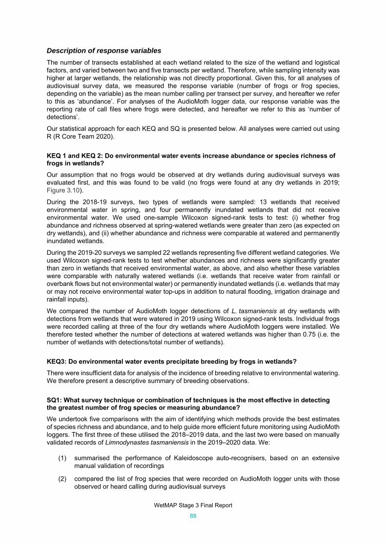
WetMAP Stage 3 Final Report
88
Description of response variables
The number of transects established at each wetland related to the size of the wetland and logistical factors, and varied between two and five transects per wetland. Therefore, while sampling intensity was higher at larger wetlands, the relationship was not directly proportional. Given this, for all analyses of audiovisual survey data, we measured the response variable (number of frogs or frog species, depending on the variable) as the mean number calling per transect per survey, and hereafter we refer to this as ‘abundance’. For analyses of the AudioMoth logger data, our response variable was the reporting rate of call files where frogs were detected, and hereafter we refer to this as ‘number of detections’.
Our statistical approach for each KEQ and SQ is presented below. All analyses were carried out using R (R Core Team 2020).
KEQ 1 and KEQ 2: Do environmental water events increase abundance or species richness of frogs in wetlands?
Our assumption that no frogs would be observed at dry wetlands during audiovisual surveys was evaluated first, and this was found to be valid (no frogs were found at any dry wetlands in 2019; Figure 3.10).
During the 2018-19 surveys, two types of wetlands were sampled: 13 wetlands that received environmental water in spring, and four permanently inundated wetlands that did not receive environmental water. We used one-sample Wilcoxon signed-rank tests to test: (i) whether frog abundance and richness observed at spring-watered wetlands were greater than zero (as expected on dry wetlands), and (ii) whether abundance and richness were comparable at watered and permanently inundated wetlands.
During the 2019-20 surveys we sampled 22 wetlands representing five different wetland categories. We used Wilcoxon signed-rank tests to test whether abundances and richness were significantly greater than zero in wetlands that received environmental water, as above, and also whether these variables were comparable with naturally watered wetlands (i.e. wetlands that receive water from rainfall or overbank flows but not environmental water) or permanently inundated wetlands (i.e. wetlands that may or may not receive environmental water top-ups in addition to natural flooding, irrigation drainage and rainfall inputs).
We compared the number of AudioMoth logger detections of L. tasmaniensis at dry wetlands with detections from wetlands that were watered in 2019 using Wilcoxon signed-rank tests. Individual frogs were recorded calling at three of the four dry wetlands where AudioMoth loggers were installed. We therefore tested whether the number of detections at watered wetlands was higher than 0.75 (i.e. the number of wetlands with detections/total number of wetlands).
KEQ3: Do environmental water events precipitate breeding by frogs in wetlands?
There were insufficient data for analysis of the incidence of breeding relative to environmental watering. We therefore present a descriptive summary of breeding observations.
SQ1: What survey technique or combination of techniques is the most effective in detecting the greatest number of frog species or measuring abundance?
We undertook five comparisons with the aim of identifying which methods provide the best estimates of species richness and abundance, and to help guide more efficient future monitoring using AudioMoth loggers. The first three of these utilised the 2018–2019 data, and the last two were based on manually validated records of Limnodynastes tasmaniensis in the 2019–2020 data. We:
(1) summarised the performance of Kaleidoscope auto-recognisers, based on an extensive manual validation of recordings
(2) compared the list of frog species that were recorded on AudioMoth logger units with those observed or heard calling during audiovisual surveys

WetMAP Stage 3 Final Report
89
(3) examined whether there was seasonal or diel variability in calling activity for five species for which there were sufficient data
(4) examined the relationship between estimates of call activity of L. tasmaniensis from AudioMoth loggers and estimates of abundance obtained from audiovisual surveys on the same day
(5) tested whether the number of detections of L. tasmaniensis varied between AudioMoth logger housings.
Comparisons 1–3 did not require statistical analysis and were based on summaries of the data. We used a Spearman’s rank correlation for Comparison 4. For Comparison 5, we used data from the nine transects across seven wetlands at which both housings were used in concert, and tested whether detections differed between housing types (fixed effect), using a zero-inflated negative binomial model with wetland as a random effect, which was fitted using the glmmTMB package in R (R Core Team 2020). Model fit was examined via QQ and residual plots, and predictions extracted and back-transformed to the original measurement scale of the response.
Preliminary evidence towards longer-term KEQs and SQs
As a preliminary evaluation of longer-term KEQs and SQs, we examined the relationship between frog responses and select hydrological variables. We considered three hydrological predictors: proportion of the wetland that was wet (wet proportion), duration of inundation (number of days above our inundation threshold), and the time since the wetland was dry (for samples with water, this was the number of days since the wet proportion was zero; for samples when the wetland was dry, this was set to zero). These were selected based on our predictions about how the frequency and duration of inundation might affect frog numbers and richness (Figures 3.2–3.5). We calculated wet proportion on the day of sampling, and the mean value of wet proportion over each of the 30-, 90-, 180- and 360-day antecedent periods, as well as duration of inundation over these four time periods (i.e. the proportion of the preceding 30/90/180/360 days that the wetland was inundated).
While the water requirements of frog species vary, most need water to persist for at least one to several months around breeding for sites to be suitable (Wassens 2011); our selected periods encapsulate this range. Wet proportion and duration of inundation were strongly correlated (Pearson’s r > 0.80) at all four antecedent periods, as was wet proportion in the previous 360 days and time since the wetland was dry. Therefore, we focused our analyses on describing the relationship between frog responses (abundance of all frogs, and each species individually) and wet proportion over different antecedent time periods.
We also examined relationships between frog responses and electrical conductivity and four variables that describe the habitat structure of the wetland fringing habitat (cover of bare ground, short herbs and grasses, short emergent vegetation and tall emergent vegetation). These variables have been shown to affect frog occupancy and abundance (e.g. Wassens 2011; Wassens and Maher 2011; Brown and Bayes 2019), and we predicted that they could also modify the relationship between frog responses and hydrology (Figures 3.2–3.5).
To explore the potential influence of landscape complexity, we included the number of waterbodies within 1 km of each wetland as a predictor in our modelling (Appendix 6 Figure A6.1).
For five response variables (abundance of all frogs, and abundances of Crinia parinsignifera, Limnodynastes dumerilii, L. tasmaniensis and Litoria peronii) we used generalised additive mixed models (GAMMs; Pedersen et al. 2019) to explore relationships with predictors. Because we had some missing values (i.e. due to unreliable water quality equipment or habitat surveys not being undertaken on all dates), we created three subsets of the data that included the complete cases for hydrological variables, electrical conductivity, and habitat structural variables, respectively. Our model fitting for each frog response variable followed the procedure presented below, with wetland and year included as random effects:
(1) run models for each hydrological predictor and number of waterbodies within 1 km individually and a null (intercept-only) model

WetMAP Stage 3 Final Report
90
(2) run two models, one of which included electrical conductivity, and the second an intercept-only model
(3) run models with the four habitat variables and a null model
(4) select the best-fitting model from Step 1, which outlines the antecedent period during which frog responses are most strongly related to wet proportion. Run subsequent models that include the best hydrological predictor, and the best other individual predictor (our dataset only supported two predictors to be included simultaneously). Models for this step used datasets that had complete cases (e.g. for models with hydrological and habitat variables, where dataset had complete cases for both sets of variables).
All model comparisons were based on Akaike information criterion values (AIC, an estimator of prediction error and thus the relative quality of models) corrected for small sample sizes. The five response variables were log-transformed before analysis to improve normality, and models used a Gaussian error distribution; residuals and QQ plots were examined for all models to ensure assumptions were met. Model predictions were extracted for all models, with predictors made at the mean value of the second predictor in multi-predictor models; predictions are presented back-transformed to the original measurement scale of the response. All models were fitted using the gamm4 package in R (R Core Team 2020).
We did not analyse species richness because more than two-thirds of the study wetlands yielded three to six species.
Our datasets for Crinia signifera and Limnodynastes fletcheri had a high number of zeros (e.g. C. signifera was not present in ~67% of samples). Thus, for these two species, we used a binomial mixed-effects model to determine the probability of occurrence as a function of wet proportion at each of the different antecedent periods, with wetland and year included as random effects as above, using the glmer function in R. Model fit was examined and predictions extracted as above.
Results
Frog occurrence/distribution
Audiovisual surveys during 2018–2020 yielded 10 frog species, four from the Family Limnodynastidae (Australian ground frogs), three from the Family Myobatrachidae (Australian toadlets and froglets), and three from the family Hylidae (tree frogs). The occurrence of species by wetland is presented in Table 3.2. Four species (Crinia parinsignifera, Limnodynastes dumerilii, L. tasmaniensis, Litoria peronii) were very widespread, being recorded from at least 23 study wetlands; four other species were seldom recorded, being recorded from only one or two study wetlands. Tahbilk Lagoon registered the most frog species (8), Lake Bael Bael the least (2). Overall, AudioMoth loggers recorded eight species during 2018–2019, all of which were also variously recorded during audiovisual surveys. Given the geographical scope of the study, not all species were expected at all study wetlands.

WetMAP Stage 3 Final Report
91
Table 3.2: WetMAP Frog monitoring: species composition per wetland for 2018–2020 audiovisual surveys. Species codes: Crin parin Crinia parinsignifera, Crin signif C. signifera, Geoc victor Geocrinia victoriana, Lim dumer Limnodynastes dumerilii, Lim fletch L. fletcheri, Lim tasman L. tasmaniensis, Lit ewing Litoria ewingii, Lit peron L. peronii, Lit ranif L. raniformis, Neo pictus Neobatrachus pictus.
Wetland Crin parin
Crin signif
Geoc victor
Lim dumer
Lim fletch
Lim tasman
Lit ewing
Lit peron
Lit ranif
Neo pictus
Total species
Black Swamp 5
Carapugna 3
Cowanna Billabong
5
Crow Swamp 4
Ducksfoot Lagoon 5
Gaynor Swamp 5
Horseshoe Lagoon (Trawool)
6
Johnsons Swamp 6
Kings Billabong 6
Kinnairds East 6
Kinnairds West 6
Lake Bael Bael 2
Lake Murphy 6
Little Lake Meran 4
McDonalds Swamp
5
Neds Corner Central
3
Neds Corner East 6
Neds Corner Woolshed
3
Nyah Floodplain 3
Reedy Swamp (Shepparton)
3
Richardson’s Lagoon
6
Tahbilk Lagoon 8
Wallpolla Horseshoe Lagoon
7
Wirra-Lo Brolga Swamp
5
Wirra-Lo Duck Creek
6
Wirra-Lo Lignum Swamp North
6
Total wetlands 24 12 1 23 16 26 2 23 2 2

WetMAP Stage 3 Final Report
92
Do environmental water events increase abundance or species richness of frogs in wetlands? (KEQ 1 and KEQ 2)
Species richness and abundance of all frogs was higher than zero at watered wetlands (Figures 3.9–3.10; Wilcoxon signed-rank test, p < 0.05) during audiovisual surveys. This result was consistent across all comparisons in both 2018-19 and 2019-20 (Figures 3.9–3.10), except for Crinia signifera (p = 0.19) and Limnodynastes fletcheri (p = 0.05) in 2019-20. In 2018-19, there were no differences in species richness or abundance between watered wetlands and those wetlands with permanent water (Figure 3.9, p > 0.05), other than for Litoria peronii, which was more abundant at permanent wetlands (Figure 3.9h, p = 0.01). In 2019-20, richness and abundance of all species was comparable at watered, permanent and naturally watered wetlands (Figure 3.10, all comparisons, p > 0.05). However, it is worth noting that the median value for all response variables was higher at watered than at the one naturally watered wetland.
A total of 204 detections of Limnodynastes tasmaniensis was recorded from the five AudioMoth logger wetlands that were watered in 2019-20, in comparison with 3 detections from wetlands that were dry in 2019-20. However, the number of calls varied considerably across the five watered wetlands (138, 61, 3, 2 and 0 calls; Figure 3.11). The number of detections at watered wetlands was therefore not significantly greater than our dry wetland value of 0.75 detections/wetland (Wilcoxon signed-rank test, p = 0.07). More calls were detected from all wetlands that had water than from those that were dry (Figure 3.11), and the number of detections at wetlands watered both in 2019-20 and previously (i.e. PW + W) was statistically greater than 0.75 (Wilcoxon signed-rank test, p = 0.01).
Figure 3.9: Results from 2018 audiovisual surveys. Panels show the (a) species richness and (b) abundance of all frogs, and then abundances of individual species (c–h). Wetlands that were dry beforehand and then watered in spring (W, n = 12); permanently inundated wetlands that may receive environmental water top-ups (PER, n = 5). The response variable for all plots is the mean value/transect.

WetMAP Stage 3 Final Report
93
Figure 3.10: Results from 2019 audiovisual surveys. Panels show (a) species richness, (b) abundance of all frogs, and then abundances of individual species (c–h). The five different groups are: Dry wetlands (D, n = 5), wetlands that were naturally watered (i.e. received rainfall in spring 2019) but were dry beforehand (NAT, 1), wetlands that were previously watered and still retain water (PW, 3), wetlands that were dry beforehand and watered in spring (W, 9) and permanently inundated wetlands that may receive environmental water top-ups (PER, 4). The response variable for all plots is the mean value/transect.
Figure 3.11: Number of AudioMoth logger detections for Limnodynastes tasmaniensis in 2019. x-axis labels follow Figure 3.10. Numbers of wetlands were D = 4, NAT = 1, PW = 3, W = 5, PER = 2.

WetMAP Stage 3 Final Report
94
Do environmental water events precipitate breeding by frogs in wetlands? (KEQ 3)
There were insufficient data for analysis of the incidence of breeding (i.e. egg masses, tadpoles, metamorphs) relative to environmental watering. However, evidence of breeding was apparent at several wetlands that either had been recently watered or held water permanently, including Limnodynastes sp. egg masses (Wirra-Lo wetland complex, Wallpolla Horseshoe Lagoon, Cowanna Billabong, Black Swamp, Kinnairds Wetland West), L. dumerilii tadpoles (Crow Swamp), Litoria peronii and Crinia sp. tadpoles [Neds Corner East and Neds Corner Woolshed, Horseshoe Lagoon (Trawool)], and metamorphs of Limnodynastes fletcheri (Wirra-Lo wetland complex) and L. tasmaniensis (Neds Corner Woolshed).
What survey technique or combination of techniques is the most effective in detecting the greatest number of frog species and measuring abundance in wetlands? (SQ 1)
Performance of classifiers There was considerable variability in the performance of the advanced Kaleidoscope classifiers between species and wetlands (Figure 3.12). Sufficient detections were manually validated for four species to present for comparison. For C. signifera and Limnodynastes fletcheri, generally only a very small proportion of calls assigned to these species by the Kaleidoscope software were confirmed as true-positives following manual verification (Figure 3.12a and b). In comparison, performance was much better for L. tasmaniensis and Litoria peronii (Figure 3.12c and d) (as high as 80–100% true-positives at some wetlands). However, false-positive rates were very high, even for these species at some wetlands. For all species, there was considerable variation in auto-recogniser performance between wetlands.
Comparison of species lists from AudioMoth acoustic loggers and audiovisual surveys There was some variability in the degree of concordance between the species lists generated at the 15 wetlands at which both methods were employed in 2018–19 (Table 3.3). Species lists were identical at Carapugna, Cowanna Billabong, Wallpolla Horseshoe Lagoon and Wirra-Lo Duck Creek. In contrast, three species (C. parinsignifera, C signifera and L. peronii) were recorded during audiovisual surveys but not detected on Audiomoth logger recordings at Black Swamp and Gaynor Swamp. Three species (C. parinsignifera, C. signifera and Limnodynastes fletcheri) were also detected at Richardson’s Lagoon only during audiovisual surveys. There were also instances where species were detected only using AudioMoth loggers, including detections of C. signifera at Kings Billabong and L. dumerilii at Nyah Floodplain. There were two species that were only detected using AudioMoth loggers: Litoria ewingii at Wirra-Lo Lignum Swamp North and the threatened Sloane’s froglet C. sloanei at Lake Murphy and Nyah Floodplain.
The degree of concordance between the two methods also varied between species. Limnodynastes tasmaniensis was recorded by both survey methods at all sites, and records of the occurrence of Litoria peronii were consistent at 13 of the 15 sites. In comparison, C. parinsignifera was detected using audiovisual surveys but not on AudioMoth logger recordings at 6 of the 15 sites. This mismatch between the two methods for C. parinsignifera was even more pronounced at the transect level (Appendix 6, Table A6.1), as were the results for most species. At the transect level, two species, Limnodynastes dumerilii and L. tasmaniensis, were detected more often on AudioMoth logger recordings than during audiovisual surveys.
Seasonal and diel variability in calling activity of six species determined using acoustic loggers Analysis of acoustic recordings revealed clear peaks in calling activity for all species around mid-November (Figure 3.13). The number of detections was generally low during the day, with peaks and an intensified level of calling activity for all species between 8 pm and 3 am (Figure 3.13).

WetMAP Stage 3 Final Report
95
The relationship between estimates of call activity of Limnodynastes tasmaniensis from AudioMoth loggers and estimates of abundance during audiovisual surveys on the same day
The estimated abundance of L. tasmaniensis recorded during 2019-20 audiovisual surveys and number of detections using AudioMoth loggers were positively correlated for the days of concurrent sampling using the two survey methods (Figure 3.14; Spearman’s rank correlation = 0.67, p < 0.002).
Does the type of AudioMoth logger housing influence the number of detections of Limnodynastes tasmaniensis?
The number of detections of L. tasmaniensis from AudioMoth loggers in two different housings was comparable (Figure 3.15; p-values for ‘Cover’ term in conditional and zero-inflated sections of model were 0.16 and 0.99, respectively).
Figure 3.12: Proportion of 2018–2019 AudioMoth logger recordings that were manually validated as being true detections for (a) Crinia signifera, (b) Limnodynastes fletcheri, (c) L. tasmaniensis and (d) Litoria peronii. Boxplots show the variability at locations where multiple transects were sampled, and single black lines show values at wetlands were only one transect was sampled. For C. signifera and L. fletcheri, only wetlands with >10 manually validated calls were included. For L. peronii, between 22 and 3204 calls were validated per wetland (median 448); for L. tasmaniensis between 16 and 3376 calls were validated (median 386). Location codes in Table 3.1.

WetMAP Stage 3 Final Report
96
Table 3.3: Summary of concordance of species detection at individual transects at wetlands from AudioMoth logger sampling and audiovisual surveys 2018–2019. Values of 0 and light-green fill highlight when a species was not recorded using either method, values of 2 and dark-green fill highlight when a species was recorded as present using both methods, values of 1 and red fill highlight when audiovisual surveys detected a species and AudioMoth acoustic classifiers did not, and values of -1 and orange fill when a species was detected by AudioMoth logger acoustic classifiers but not in audiovisual surveys. Species abbreviations are C. par = Crinia parinsignifera, C. sig = Crinia signifera, C. slo= Crinia sloanei, L. dum = Limnodynastes dumerilii, L. fle = L. fletcheri, L. tas = L. tasmaniensis, L. ewi = Litoria ewingii complex, L. per = L. peroni.
Wetland C. par C. sig C. slo L. dum L. fle L. tas L. ewi L. per
Black Swamp 1 1 0 2 0 2 0 1
Carapugna 0 0 0 2 0 2 0 2
Cowanna Billabong 2 0 0 2 2 2 0 2
Crow Swamp 1 2 0 2 0 2 0 0
Ducksfoot Lagoon 2 0 0 2 1 2 0 2
Gaynor Swamp 1 1 0 2 0 2 0 1
Kings Billabong 1 –1 0 2 0 2 0 2
Kinnairds Wetland 2 2 0 1 2 2 0 2
Lake Murphy 2 2 –1 2 2 2 0 2
Little Lake Meran 1 0 0 2 0 2 0 2
Nyah Floodplain 0 0 –1 –1 2 2 0 2
Richardson’s Lagoon 1 1 0 2 1 2 0 2
Wallpolla Horseshoe Lagoon 2 2 0 2 2 2 0 2
Wirra-Lo Duck Creek 2 0 0 2 2 2 0 2
Wirra-Lo (Lignum Swamp North) 2 2 0 2 2 2 –1 2

WetMAP Stage 3 Final Report
97
Figure 3.13: Seasonal and diel variability in AudioMoth logger detections for six common frog species: (a, b) Crinia parinsignifera, (c, d) C. signifera, (e, f) Limnodynastes dumerilii, (g, h) L. fletcheri, (i, j) L. tasmaniensis, and (k, l) Litoria peronii. Grey box on ‘Day of year’ plots indicates period when AudioMoth loggers were not set.
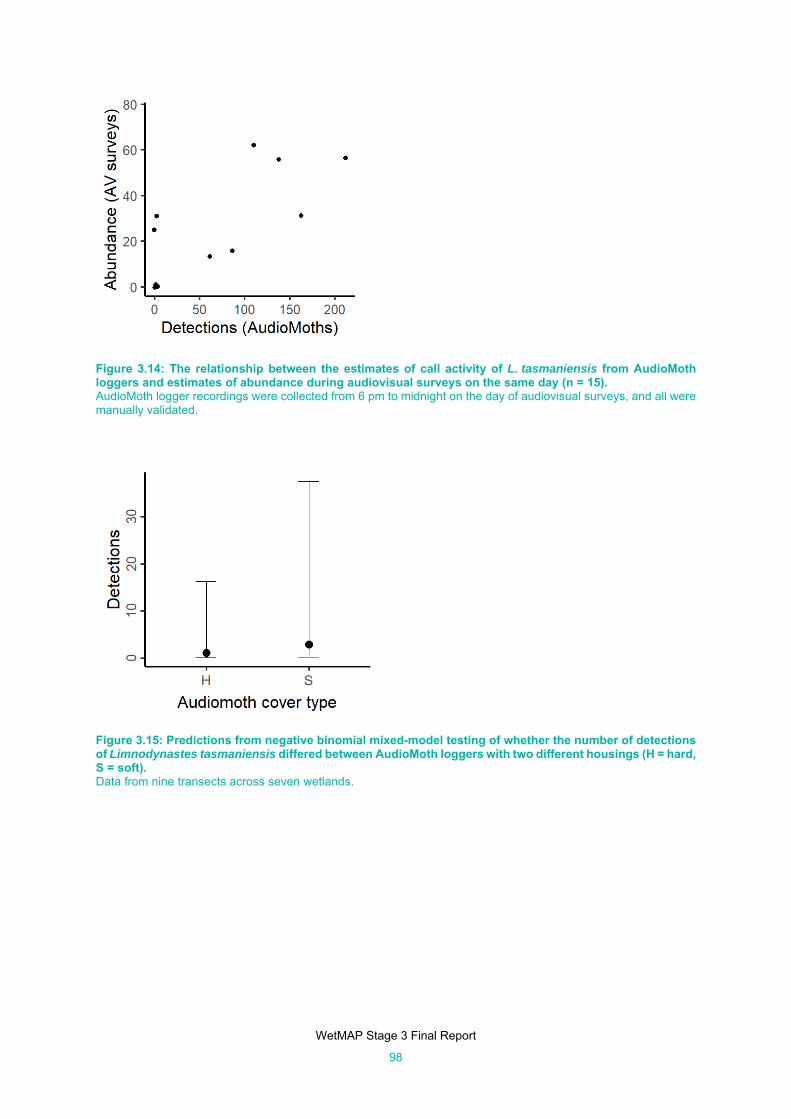
WetMAP Stage 3 Final Report
98
Figure 3.14: The relationship between the estimates of call activity of L. tasmaniensis from AudioMoth loggers and estimates of abundance during audiovisual surveys on the same day (n = 15). AudioMoth logger recordings were collected from 6 pm to midnight on the day of audiovisual surveys, and all were manually validated.
Figure 3.15: Predictions from negative binomial mixed-model testing of whether the number of detections of Limnodynastes tasmaniensis differed between AudioMoth loggers with two different housings (H = hard, S = soft). Data from nine transects across seven wetlands.

WetMAP Stage 3 Final Report
99
Exploration of frog relationships with hydrological regimes (preliminary evaluation of KEQs 4–6, SQs 2–4)
KEQ 4: To what extent does the environmental water regime in wetlands affect the abundance of all resident frog species?
KEQ 5: To what extent does the environmental water regime in wetlands affect the species richness of frogs?
KEQ 6: To what extent does the environmental water regime in wetlands affect breeding by frogs?
SQ 2: Is the composition of frog assemblages related to the timing, frequency and/or duration of environmental watering, or the legacies of water regime history? If so, to what extent do these flow characteristics increase or decrease frog species richness and abundance?
SQ 2a: Is the effect of an environmental water event on richness and abundance of frog species dependent on the hydrological history prior to the watering and over what antecedent period?
SQ 2b: Is the effect of an environmental water event on richness and abundance of frog species dependent on the timing, duration and/or frequency of the watering?
SQ 3: Is the effect of an environmental water event on richness and abundance of frog species dependent on water quality and/or habitat structure?
SQ 4: Is the effect of an environmental water event on richness and abundance of frog species dependent on landscape complexity (especially habitat connectivity and the existence of proximate potential frog refuges)?
We found a range of different relationships between frog responses, hydrological predictors and habitat variables (all model selection summaries are in Appendix 6, Tables A6.2–A6.6). The best predictor of the total abundance of all frog species was the wet proportion in the preceding 30 days (Figure 3.16a; adjusted R2 = 0.38), with an increase predicted up to a wet proportion of approximately 0.3 and then a plateau for values greater than 0.3. This effect was consistent across seasons (Table A6.2). The wet proportion in the preceding 30 days was also the best hydrological predictor for C. parinsignifera (Table A6.3), with numbers predicted to be low when the wet proportion in the preceding 30 days was below ~0.50, with an increase in frog abundance with increasing wet proportion (Figure 3.16b). However, this relationship was weak (adjusted R2 = 0.13), and a similar predictor to a null model (Table A6.3, delta AIC = 1.89). No water quality or habitat variables were better predictors of C. parinsignifera numbers than the null model.
The two best predictors of L. dumerilii numbers were tall emergent vegetation and wet proportion in the preceding 90 days (Table A6.4). Numbers were highest at intermediate levels of wet proportion in the preceding 90 days (Figure 3.16c) and tall emergent vegetation cover (Figure 3.16d). None of the hydrological predictors was a good predictor of the occurrence of Crinia signifera (all model p-values > 0.50). All models for L. fletcheri were non-significant (p > 0.05), but there was some evidence that occurrence was positively related to both wet proportion on the day of sampling and wet proportion over the 30-day antecedent period, with p-values of ~0.10 (see also Figure 3.16e). For L. tasmaniensis, the best-fitting model (Table A6.5) included wet proportion (90 days), with highest numbers at intermediate proportions (Figure 3.16g, adjusted R2 = 0.6). Numbers of L. tasmaniensis were also positively related to cover of tall emergent vegetation (Figure 3.16h). We found no evidence of any relationships between numbers of Litoria peronii and any predictors (Table A6.6).

WetMAP Stage 3 Final Report
100
Figure 3.16: Predictions for best-fitting models (Tables A6.2–A6.6) exploring the influence of hydrology and tall emergent vegetation on frog responses. Predictions are from generalised additive mixed models, other than for panel (f), which is a binomial linear mixed-effects model. The black line shows the mean prediction, and the grey shading indicates 95% confidence intervals. Note that for panels (a) and (g), the upper confidence intervals have been truncated to better show the mean responses.

WetMAP Stage 3 Final Report
101
Discussion
Response of frog abundance (KEQ1) and species richness (KEQ2) to environmental water
We found a clear response to watering by frogs, with higher abundance and species richness at wetlands that received water (but would have been dry otherwise) than dry ones. Wetlands with more consistent water also had more frogs in our comparisons of wetlands with different hydrological characteristics (intermittent-seasonal-permanent).
In general, we found a comparable number of species and frogs at temporary watered wetlands (i.e. Group 1 in 2018-19, Groups 1, 2 in 2019-20 in Table 3.1) and permanently inundated wetlands (i.e. Group 2 in 2018-19, Group 5 in 2019-20 in Table 3.1), although at least one species — Litoria peronii — was more abundant at permanently inundated wetlands.
This frog inhabits a variety of waterbodies yet prefers deeper open ponds and rarely breeds in those waterbodies that are shallow or well vegetated (Gonzalez et al. 2011; Wassens 2011). It typically shelters in tree hollows and under bark by day. It breeds successfully in permanent waterbodies and small residual ponds at those wetlands with long hydroperiods, as well as temporary floodplain reaches (Wassens & Maher 2010; Wassens 2011).
In contrast, Crinia parinsignifera is highly adaptable, has tadpoles that are generalist herbivores and detritivores, and consequently appears to be less sensitive to altered wetland hydrology (Wassens 2011). For successful breeding of C. parinsignifera, wetlands should retain pooled water for a minimum of 6 weeks if flooded during spring or summer, and 3 months if flooded in winter (Wassens 2011; Wassens and Maher 2011).
It should be noted that very few naturally watered wetlands (i.e. Group 6 in 2019-20 in Table 3.1) were included in our sample, so there is low power to evaluate inter-wetland differences. However, the dearth of naturally watered wetlands reflects the degree of floodplain regulation in northern Victoria (and the Murray–Darling Basin more generally); this means that finding more suitable naturally watered wetlands to increase our statistical power in the future will be challenging.
Past studies have found significant associations of species and trophic guilds with inundation at both the wetland scale and floodplain scale, and in the semi-arid landscape of south-eastern Australia the availability of water was often the key driver of frog occupancy, calling and microhabitat use (Amos 2017; Bino et al. 2018; Hoffmann 2018).
Response of frog breeding to environmental water (KEQ 3) All frog species known from northern Victoria breed opportunistically after flooding of wetlands. Breeding is usually immediate and tadpole development largely synchronous and rapid; most frog species metamorphose 3–4 months after inundation, a pattern documented for other parts of the Murray River floodplain (Hoffmann 2018).
Few instances of breeding were recorded during the 2018–2020 surveys, yet we confirmed some breeding for species of the Crinia, Limnodynastes and Litoria genera at several wetlands, each of which had either been recently watered or held water permanently. Tadpoles could not be identified to species when not ‘in hand’.
Our results suggest limited reproduction, although our survey methods, which focused on adult frogs, were not specific or intensive enough to generate breeding records. Most tadpole survey methods are especially inefficient in large complex wetlands, such as those that WetMAP is centred on, or are otherwise cost-prohibitive when low detection probabilities and required levels of replication are considered (Wassens et al. 2017). If breeding is considered a crucial response to environmental watering that must be monitored, then a review of the current methodological approach is warranted.

WetMAP Stage 3 Final Report
102
Determining the most effective survey methods to measure frog species richness and abundance (SQ 1)
To improve the chances of recording the full frog assemblage at wetlands, multiple survey techniques are often employed in concert. The integration of complementary survey techniques can be very effective (Browning et al. 2017; Wassens et al. 2017).
We employed audiovisual surveys as well as a passive recording technique (AudioMoth acoustic logger) at each monitoring transect, and this approach resulted in a greater number of frog taxa per wetland than either technique would have delivered on its own. With a revised methodological approach and further refinement of call classifiers, we anticipate even greater efficiency in identifying resident frog assemblages.
AudioMoth acoustic monitoring We have made considerable progress in developing the technology for processing the data from AudioMoth loggers, for monitoring frog responses to environmental flows. A major outcome was confirming that AudioMoth loggers can detect additional species to those found during audiovisual surveys, exemplified by the detection of the nationally threatened Sloane’s froglet (Crinia sloanei) at Lake Murphy and Nyah Floodplain in 2018–2019. AudioMoth loggers offer the ability to acquire data to compare both immediate and longer-term responses to management actions like environmental watering. This cannot be achieved through audiovisual surveys alone, without a massive and likely cost-prohibitive increase in effort.
We observed some differences between the species that were detected using AudioMoth loggers and audiovisual surveys. Similar variability has been observed in other studies comparing AudioMoth loggers and other sampling methods (e.g. Schroeder and McRae 2020). There are several potential explanations for these differences, including: (i) automatic recorders are stationary and only able to capture acoustically active species within the limited range of the logger; (ii) configuration of recorder settings (e.g. timing and length of recording period, direction of microphone, distance relative to signal) will determine which species are recorded; (iii) other sounds (e.g. calls from other species, ambient environmental noise) may obscure calls; and (iv) only a single audiovisual survey was conducted at each transect. Increasing replication with repeat visits may mean that there is greater concordance between the two methods (especially for species that were calling at wetlands but perhaps not calling during the one-off surveys). Despite the potential influence of these factors, the two survey methods generally yielded similar results, both in terms of species lists and in ‘abundance’ (e.g. number of detections of L. tasmaniensis from AudioMoth loggers and estimates of abundance from audiovisual surveys) on the same day.
We found variability in the performance of recognisers both among species and between wetlands for the same species. Similar variability has been observed in international studies (Schroeder and McRae 2020), as well as in The Living Murray program in Barmah Forest (Durkin and Howard 2020). Several factors can influence recogniser performance: intraspecific variability in calls has been observed both between and within locations (e.g. Crump and Houlahan 2017; Xie et al. 2018); in addition, vocally active fauna species diversity can vary between wetlands, and these non-target species can produce similar sounds that obscure the species calls of interest; furthermore, detection distances (Browning et al. 2017), along with wetland-specific environmental factors [e.g. medium (air/water), temperature, pressure, humidity, ambient sound levels, habitat structure] also affect detection power.
AudioMoth units are small (match-box-sized) loggers that are supplied without housing, so protection (of circuitry, micro card and batteries) is required when deploying them in exposed field locations. There was no significant difference in call detection between the ‘hard’ and the ‘soft’ housing, suggesting that the cheaper and simpler soft housing of a zip-lock plastic bag inside shade cloth is preferable.
Three avenues of work could help refine future sampling and AudioMoth logger methodological development. First, we can use our results showing seasonal and diel peaks in frog calling activity to better target sampling periods. Our detections were highest between 9 pm and 2 am, supporting the current timing of audiovisual surveys. Being able to target times to get a good representation of calling activity on an individual day will help reduce data collection and processing time.
The second avenue for future work is to evaluate ways to minimise the time involved in processing call recordings, and maximise the precision, accuracy and reliability of results, a common problem affecting

WetMAP Stage 3 Final Report
103
bioacoustics programs globally (Gibb et al. 2019). The Kaleidoscope software is very user-friendly, yet it requires considerable manual validation of detections, and there are difficulties when the species of interest calls infrequently or has calls that are not easily distinguished from other environmental sounds.
The field of bioacoustics monitoring is developing rapidly, and emerging technology and techniques potentially offer marked improvements in data processing time, and the precision, accuracy and reliability of results; in addition, they may be more suitable for detecting multiple species, including those that are vocally rare or have different call dialects. These approaches include machine-learning (Balantic and Donovan 2020) and deep-learning/convolutional neural network methods (LeBien et al. 2020). We now have a dataset that could form the basis of future work to evaluate some of these methods.
The third avenue for future work is to consider more sophisticated methods for statistical analysis, for example, dynamic occupancy modelling (e.g. Balantic and Donovan 2019). These methods would allow us to better interpret the presence of species at wetlands (i.e. provide more certainty around which detections are true-positives) and call intensity data, and also allow us to simultaneously address methodological considerations and test how species occurrence and activity relate to hydrological predictors related to environmental watering.
Preliminary evaluation of longer-term KEQs and SQs Our study revealed relationships for most frog species with some hydrological predictors, typically related to the extent and duration of inundation. However, the importance of the antecedent watering period varied: total abundance across all species and abundance of Crinia parinsignifera were correlated with ‘wet proportion 30 days’, whereas the best predictor for Limnodynastes dumerilii was ‘wet proportion 90 days’. These antecedent periods accord with general tadpole development times for both C. parinsignifera and L. dumerilii, which are variable, influenced by water temperature, changing water level and food availability. The development of C. parinsignifera generally takes 6 weeks to 3 months, and 3–6 months for L. dumerilii (Wassens 2011; Anstis 2017).
The responses of all of the study frog species to hydrological variables and tall emergent vegetation, while mostly reflecting a positive response, varied in strength. A positive response was found for total abundance and the abundance of C. parinsignifera, and the highest numbers of L. dumerilii and L. tasmaniensis were observed at intermediate water levels. The abundance of L. dumerilii and the probability of occurrence for L. fletcheri both increased with increasing hydroperiod (Figure 3.16), which accords with previous findings (Wassens and Maher 2011). Limnodynastes fletcheri prefers wetlands with longer hydroperiods and generally occurs only if there is permanent water nearby (Wassens 2011).
We need a better understanding of eco–hydrological relationships by collecting specific data, aligned with the fundamental influences on frog occurrence presented in our broad conceptual models (Figures 4.1 and 4.2). This has implications for wetland selection — incorporating additional wetlands to encompass select hydrological regimes and counterfactuals —and the environmental data we collect. The relationships between frog occurrence and environmental characteristics are inconsistent, so broadening the dataset to include additional study wetlands and the further surveying of existing study wetlands will yield data that more precisely identify the most influential drivers of frog occurrence.
Our modelling was limited to a subset of measured/estimated habitat variables, yet it demonstrated that some variables, notably tall emergent vegetation, influenced frog occurrence. This suggests that a more complete analysis will likely identify additional influential attributes. Further attention should be given to water quality and the habitat characteristics of the aquatic and fringing terrestrial habitat zones, as well as a more sophisticated evaluation of the degree to which landscape-scale complexity affects frog occurrence and dispersal. Consequently, environmental watering will probably need to be undertaken with complementary management actions that support the maintenance or enhancement of select terrestrial habitat features. Tall emergent vegetation featured in several models for Limnodynastes species, confirming the significance of this aquatic feature found in other studies in south-eastern Australia (e.g. Wassens and Maher 2011).
The water quality measurements used in our modelling, particularly relating to electrical conductivity, were irregular, probably caused by defective equipment. This unreliability meant that measurements to date were excluded from analysis. Future surveys will include the collection of more reliable water quality measurements.

WetMAP Stage 3 Final Report
104
Landscape complexity affects the distribution and occurrence of frogs, especially in alienated landscapes of the sort common across northern Victoria. Many physiographic elements are known or expected to influence the capacity of frogs to occupy or move around landscapes prone to changing water regimes, and these include topography (Westgate et al. 2012), quality of the landscape matrix (e.g. Quesnelle et al. 2015), and the number and proximity of neighbouring wetlands (e.g. Hamer and Mahony 2010; Heard et al. 2013; Ishiyama et al. 2014; Uden et al. 2014). Landscape connectivity or resistance is important for dispersal and gene flow, and thus related to the life-history traits and movement capacity of individual frog species (Richardson 2012; Watts et al. 2015; Howell et al. 2018). Landscape complexity can also facilitate the spread of invasive species, which has implications for competition, predation, and the incidence of disease (particularly chytridiomycosis) (Cohen et al. 2019; Pulsford et al. 2019).
Connectivity will assume greater importance as climate changes to a regime of lower rainfall and likely increased habitat fragmentation. Thus, the incorporation of both ephemeral and permanent habitat patches should be incorporated into conservation and management plans to benefit dispersive frog species like the Growling Grass Frog Litoria raniformis (e.g. Wassens et al. 2007; Wassens et al. 2008) and likely many other frog taxa.
Conclusions and future directions WetMAP Stage 3 demonstrated support for elements of our conceptual models that predicted environmental watering can increase frog occurrence in wetlands. Specifically, we revealed the short-term benefits of environmental water to frog occurrence and abundance, the corollary of which is that we are now prepared to explore the water regime requirements of frog assemblages. This will include an understanding of optimal water regimes, which will vary by taxa and probably geographic location, as well as response thresholds to a single event or regime (e.g. timing and duration of an event, frequency of events). Some frog species are known to be less sensitive to variations in wetland hydrology than other wetland-dependent species, yet the timing and duration of watering are expected to influence the occurrence of all frog taxa most markedly. We observed greater frog species richness and abundance in those wetlands that experienced seasonal watering and drawdown than those with less frequent watering or permanent water (at reasonably consistent levels).
Stage 3 results also provided evidence for refining the monitoring approach, including the collection of survey data and its processing. Future monitoring will be more efficient in the field and provide improvements in data processing time as well as the reliability of results.
As for other WetMAP themes, the next step for the frog theme will be a re-evaluation of the KEQs and SQs to guide the next stage of the project. Many of the questions can hopefully be answered, at least partly, using AudioMoths, which provide the ability to collect high-temporal-resolution, long-term data from a wider range of wetlands. Further development of this methodology is important. For example, the application of machine-learning innovations to automated frog call identification is a promising way forward (e.g. Gan et al. 2019; Gibb et al. 2019), and one that ARI is currently exploring with the aim of streamlining call identification with increased accuracy.
Our focus has been on evaluating responses to environmental water events in this phase, primarily through comparing frog abundance and richness at watered wetlands with those at wetlands that are dry. However, more nuanced comparisons are needed; for example, examining frog responses to watering at wetlands that retain water for much or all of the time and receive watering top-ups. This will likely require the incorporation of other experimental designs (e.g. before–after control–impact) or collecting information to develop modelled counterfactuals against which to compare frog responses.
Another important next step would be to further our understanding of the mechanisms via which frogs respond to environmental watering, and factors that might modify these responses. Reviewing and updating our conceptual models will be important, to identify which links in our current models that have not yet been explored should be prioritised.
It is acknowledged that large-scale factors, such as the spatial arrangement of waterbodies, along with finer-scale parameters, such as hydrology, vegetation, predator abundance and disease, will affect frog responses. Therefore, combining scale-related parameters, such as landscape context (e.g. connectivity, matrix) and chytridiomycosis, along with an assessment of the impacts of watering on habitat availability, may also be considered for the next phase.

WetMAP Stage 3 Final Report
105
References Alroy, J. (2015). Current extinction rates of reptiles and amphibians. Proceedings of the National
Academy of Sciences of the United States of America 112, 13003–13008.
Amos, C. (2017). Response of frogs to environmental factors at multiple scales in the Lachlan Catchment of New South Wales. PhD thesis, Charles Sturt University, Victoria.
Anstis, M. (2017). Tadpoles and frogs of Australia. 2nd edn. New Holland, Chatswood, New South Wales
Auffret, A.G., Plue, J. and Cousins, S.A.O. (2015). The spatial and temporal components of functional connectivity in fragmented landscapes. Ambio 44, 51–59.
Balantic, C. and Donovan, T. (2019). Dynamic wildlife occupancy models using automated acoustic monitoring data. Ecological Applications 29, e01854.
Balantic, C.M. and Donovan, T.M. (2020). Statistical learning mitigation of false positives from template-detected data in automated acoustic wildlife monitoring. Bioacoustics 29, 296–321.
Bellard, C., Genovesi, P. and Jeschke, J.M. (2016). Global patterns in threats to vertebrates by biological invasions. Proceedings of the Royal Society B: Biological Sciences 283, 20152454.
Bino, G., Wassens, S., Kingsford, R.T., Thomas, R.F. and Spencer, J. (2018). Floodplain ecosystem dynamics under extreme dry and wet phases in semi-arid Australia. Freshwater Biology 63, 224–241.
Brown, G. and Bayes, E. (2019). WetMAP Frog Theme Annual Report 2018–19. Unpublished report for Water and Catchments Division, DELWP. Arthur Rylah Institute for Environmental Research, Department of Environment, Land, Water and Planning, Heidelberg, Victoria.
Brown, G.W., Scroggie, M.P., Smith, M.J. and Steane, D. (2007). An evaluation of methods for monitoring the population status of the threatened Alpine Tree Frog Litoria verreauxii alpina in south-eastern Australia. Copeia 2007, 766–771.
Browning, E., Gibb, R., Glover-Kapfer, P. and Jones, K. (2017). Passive acoustic monitoring in ecology and conservation. WWF Conservation Technology Series 1(2). WWF-UK, Woking, UK.
Ceballos, G., Ehrlich, P.R. and Dirzo, R. (2017). Biological annihilation via the ongoing sixth mass extinction signaled by vertebrate population losses and declines. Proceedings of the National Academy of Sciences of the United States of America 114, E6089–E6096.
Cogger, H.G. (2018). Reptiles and amphibians of Australia, updated 7th edn. CSIRO Publishing, Collingwood, Victoria.
Cohen, J.M., Civitello, D.J., Venesky, M.D., McMahon, T.A. and Rohr, J.R. (2019). An interaction between climate change and infectious disease drove widespread amphibian declines. Global Change Biology 25, 927–937.
Crump, P.S. and Houlahan, J. (2017). Designing better frog call recognition models. Ecology and Evolution 7, 3087–3099.
Cushman, S.A. (2006). Effects of habitat loss and fragmentation on amphibians: A review and prospectus. Biological Conservation 128, 231-240.
Department of Environment Land Water and Planning. (2016). The Victorian wetland classification framework 2014. Department of Environment, Land, Water and Planning, East Melbourne, Victoria.
Durkin, L. and Howard, K. (2020). The Living Murray – Frog Condition Monitoring in Gunbower Forest. Unpublished Client Report for the North Central Catchment Management Authority. Arthur Rylah Institute for Environmental Research, Department of Environment, Land, Water and Planning, Heidelberg, Victoria.
Fardell, L., Valdez, J., Klop-Toker, K., Stockwell, M., Clulow, S., Clulow, J. and Mahony, M. (2018). Effects of vegetation density on habitat suitability for the endangered Green and Golden Bell Frog, Litoria aurea. Herpetological Conservation and Biology 13, 47–57.

WetMAP Stage 3 Final Report
106
Fordham, D.A., Brook, B.W., Hoskin, C.J., Pressey, R.L., VanDerWal, J. and Williams, S.E. (2016). Extinction debt from climate change for frogs in the wet tropics. Biology Letters 12, 20160236.
Gan, H., Zhang, J., Towsey, M., Truskinger, A., Stark, D., van Rensburg, B., Li, Y. and Roe, P. (2019). Recognition of frog chorusing with acoustic indices and machine learning. In: Gupta, A (Ed.) Proceedings of the 2019 15th International Conference on eScience, pp. 106–115. The Institute of Electrical and Electronics Engineers, San Diego, CA, USA.
Gervasi, S.S., Stephens, P.R., Hua, J., Searle, C.L., Xie, G.Y., Urbina, J., Olson, D.H., Bancroft, B.A., Weis, V., Hammond, J.I., Relyea, R.A. and Blaustein, A.R. (2017). Linking ecology and epidemiology to understand predictors of multi-host responses to an emerging pathogen, the amphibian chytrid fungus. PLoS ONE 12, e0167882.
Gibb, R., Browning, E., Glover-Kapfer, P. and Jones, K.E. (2019). Emerging opportunities and challenges for passive acoustics in ecological assessment and monitoring. Methods in Ecology and Evolution 10, 169–185.
Gillespie, G.R., Hunter, D., Hollis, G., Scheele, B. and West, M. (2018). A tale of threatened frogs: demonstrating the value of long-term monitoring. In: Legge, S., Robinson, N., Lindenmayer, D., Scheele, B., Southwell, D. and Wintle, B. (Eds) Monitoring Threatened Species and Ecological Communities, pp. 165–177. CSIRO Publishing, Clayton, Victoria.
Gillespie, G.R., Roberts, J.D., Hunter, D., Hoskin, C.J., Alford, R.A., Heard, G.W., Hines, H., Lemckert, F., Newell, D. and Scheele, B.C. (2020). Status and priority conservation actions for Australian frog species. Biological Conservation 247, 108543.
Grant, E.H.C., Miller, D.A.W. and Muths, E. (2020). A synthesis of evidence of drivers of amphibian declines. Herpetologica 76, 101–107.
Green, D.M., Lannoo, M.J., Lesbarrères, D. and Muths, E. (2020). Amphibian population declines: 30 years of progress in confronting a complex problem. Herpetologica 76, 97–100, 104.
Hale, J.M., Heard, G.W., Smith, K.L., Parris, K.M., Austin, J.J., Kearney, M. and Melville, J. (2013). Structure and fragmentation of growling grass frog metapopulations. Conservation Genetics 14, 313–322.
Hamer, A.J., Heard, G.W., Urlus, J., Ricciardello, J., Schmidt, B., Quin, D. and Steele, W.K. (2016). Manipulating wetland hydroperiod to improve occupancy rates by an endangered amphibian: modelling management scenarios. Journal of Applied Ecology 53, 1842–1851.
Hamer, A.J. and Mahony, M.J. (2010). Rapid turnover in site occupancy of a pond-breeding frog demonstrates the need for landscape-level management. Wetlands 30, 287–299.
Hamer, A.J. and Parris, K.M. (2013). Predation modifies larval amphibian communities in urban wetlands. Wetlands 33, 641–652.
Hazell, D. (2003). Frog ecology in modified Australian landscapes: a review. Wildlife Research 30: 193-205.
Healey, M., Thompson, D. and Robertson, A. (1997). Amphibian communities associated with billabong habitats on the Murrumbidgee floodplain, Australia. Australian Journal of Ecology 22, 270–278.
Heard, G.W., Canessa, S. and Parris, K.M. (2015a). Interspecific variation in the phenology of advertisement calling in a temperate Australian frog community. Ecology and Evolution 5, 3927–3938.
Heard, G.W., McCarthy, M.A., Scroggie, M.P., Baumgartner, J.B. and Parris, K.M. (2013). A Bayesian model of metapopulation viability, with application to an endangered amphibian. Diversity and Distributions 19, 555–566.
Heard, G.W., Scroggie, M.P., Clemann, N. and Ramsey, D.S.L. (2014). Wetland characteristics influence disease risk for a threatened amphibian. Ecological Applications 24, 650–662.
Heard, G.W., Scroggie, M.P. and Malone, B.S. (2012). Classical metapopulation theory as a useful paradigm for the conservation of an endangered amphibian. Biological Conservation 148, 156–166.

WetMAP Stage 3 Final Report
107
Heard, G.W., Thomas, C.D., Hodgson, J.A., Scroggie, M.P., Ramsey, D.S.L. and Clemann, N. (2015b). Refugia and connectivity sustain amphibian metapopulations afflicted by disease. Ecology Letters 18, 853–863.
Hill, A.P., Prince, P., Piña Covarrubias, E., Doncaster, C.P., Snaddon, J.L. and Rogers, A. (2018). AudioMoth: Evaluation of a smart open acoustic device for monitoring biodiversity and the environment. Methods in Ecology and Evolution 9, 1199–1211.
Hirschfeld, M., Blackburn, D.C., Doherty-Bone, T.M., Gonwouo, L.N., Ghose, S. and Rödel, M.-O. (2016). Dramatic declines of montane frogs in a central African biodiversity hotspot. PLoS ONE 11, e0155129-e0155129.
Hoffmann, E.P. (2018). Environmental watering triggers rapid frog breeding in temporary wetlands within a regulated river system. Wetlands Ecology and Management 26, 1073–1087.
Howell, P.E., Hossack, B.R., Muths, E., Sigafus, B.H. and Chandler, R.B. (2020). Informing amphibian conservation efforts with abundance-based metapopulation models. Herpetologica 76, 240–250, 211.
Howell, P.E., Muths, E., Hossack, B.R., Sigafus, B.H. and Chandler, R.B. (2018). Increasing connectivity between metapopulation ecology and landscape ecology. Ecology 99, 1119–1128.
Hunter, D., Clemann, N., Coote, D., Gillespie, G., Hollis, G., Scheele, B.C., Phillips, A. and West, M. (2018). Frog declines and associated management response in south-eastern mainland Australia and Tasmania. In: Heatwole, H. and Rowley, J.J.L. (Eds) Status of Conservation and Decline of Amphibians: Australia, New Zealand and Pacific Islands, pp. 39–56. CSIRO Publishing, Clayton South, Victoria.
Hunter, D.A., Smith, M.J., Scroggie, M.P. and Gilligan, D. (2011). Experimental examination of the potential for three introduced fish species to prey on tadpoles of the endangered Booroolong Frog, Litoria booroolongensis. Journal of Herpetology 45, 181–185.
Ishiyama, N., Akasaka, T. and Nakamura, F. (2014). Mobility-dependent response of aquatic animal species richness to a wetland network in an agricultural landscape. Aquatic Sciences 76, 437–449.
Jansen, A. and Healey, M. (2003). Frog communities and wetland condition: relationships with grazing by domestic livestock along an Australian floodplain river. Biological Conservation 109, 207–219.
Júnior, V.B. and Rocha, C.F. (2017). Tropical tadpole assemblages: Which factors affect their structure and distribution? Oecologia Australis 17, 12.
Kolby, J.E. (2018). Amphibia: Global amphibian declines caused by an emerging infectious disease and inadequate immune responses. In: Cooper, E.L. (Ed.) Advances in Comparative Immunology, pp. 981–990. Springer International Publishing, Cham.
LeBien, J., Zhong, M., Campos-Cerqueira, M., Velev, J.P., Dodhia, R., Ferres, J.L. and Aide, T.M. (2020). A pipeline for identification of bird and frog species in tropical soundscape recordings using a convolutional neural network. Ecological Informatics 59, 101113.
Lemckert, F. and Mahony, M. (2018). The status of decline and conservation of frogs in temperate coastal south-eastern Australia. In: Heatwole, H. and Rowley, J.J.L. (Eds) Status of Conservation and Decline of Amphibians: Australia, New Zealand and Pacific Islands, pp. 59–72. CSIRO Publishing, Clayton South, Victoria.
Levins, R. (1969). Some demographic and genetic consequences of environmental heterogeneity for biological control. Bulletin of the Entomological Society of America 15, 237–240.
Levins, R. (1970). Extinction. In: Gesternhaber, M. (Ed.) Some Mathematical Problems in Biology. American Mathematical Society, Rhode Island.
Linke, S. and Deretic, J.-A. (2020). Ecoacoustics can detect ecosystem responses to environmental water allocations. Freshwater Biology 65, 133–141.

WetMAP Stage 3 Final Report
108
Lips, K.R. (2016). Overview of chytrid emergence and impacts on amphibians. Philosophical Transactions of the Royal Society B: Biological Sciences 371, 20150465.
Lowe, K., Castley, J.G. and Hero, J.-M. (2015). Resilience to climate change: complex relationships among wetland hydroperiod, larval amphibians and aquatic predators in temporary wetlands. Marine and Freshwater Research 66, 886–899.
Marques, N.C.S. and Nomura, F. (2018). Environmental and spatial factors affect the composition and morphology of tadpole assemblages. Canadian Journal of Zoology 96, 1130–1136.
McGinness, H.M., Arthur, A.D., Ward, K.A. and Ward, P.A. (2014). Floodplain amphibian abundance: responses to flooding and habitat type in Barmah Forest, Murray River, Australia. Wildlife Research 41, 149–162.
Murray, K.A., Skerratt, L.F., Marantelli, G., Berger, L., Hunter, D., Mahony, M. and Hines, H. (2011). Hygiene protocols for the control of diseases in Australian frogs. A Report for the Australian Government Department of Sustainability, Environment, Water, Population and Communities. Available from: http://www.environment.gov.au/biodiversity/invasive-species/publications/hygiene-protocols-control-diseases-australian-frogs (accessed September 2020). Department of Sustainability, Environment, Water, Population and Communities, Canberra, ACT.
O’Hanlon, S.J., Rieux, A., Farrer, R.A., Rosa, G.M., Waldman, B., Bataille, A., Kosch, T.A., Murray, K.A., Brankovics, B., Fumagalli, M., Martin, M.D., Wales, N., Alvarado-Rybak, M., Bates, K.A., Berger, L., Böll, S., Brookes, L., Clare, F., Courtois, E.A., Cunningham, A.A., Doherty-Bone, T.M., Ghosh, P., Gower, D.J., Hintz, W.E., Höglund, J., Jenkinson, T.S., Lin, C.-F., Laurila, A., Loyau, A., Martel, A., Meurling, S., Miaud, C., Minting, P., Pasmans, F., Schmeller, D.S., Schmidt, B.R., Shelton, J.M.G., Skerratt, L.F., Smith, F., Soto-Azat, C., Spagnoletti, M., Tessa, G., Toledo, L.F., Valenzuela-Sánchez, A., Verster, R., Vörös, J., Webb, R.J., Wierzbicki, C., Wombwell, E., Zamudio, K.R., Aanensen, D.M., James, T.Y., Gilbert, M.T.P., Weldon, C., Bosch, J., Balloux, F., Garner, T.W.J. and Fisher, M.C. (2018). Recent Asian origin of chytrid fungi causing global amphibian declines. Science 360, 621–627.
Ocock, J. and Wassens, S. (2018). The status of decline and conservation of frogs in the semi-arid zones of Australia. In: Heatwole, H. and Rowley, J. (Eds) Status of conservation and decline of amphibians. Australia, New Zealand and Pacific Islands, 91-106. CSIRO, Clayton South, Victoria.
Pedersen, E.J., Miller, D.L., Simpson, G.L. and Ross, N. (2019). Hierarchical generalized additive models in ecology: an introduction with mgcv. PeerJ 7, e6876.
Phillott, A.D., Speare, R., Hines, H.B., Skerratt, L.F., Meyer, E., McDonald, K.R., Cashins, S.D., Mendez, D. and Berger, L. (2010). Minimising exposure of amphibians to pathogens during field studies. Diseases of Aquatic Organisms 92, 175–185.
Potvin, D.A., Parris, K.M., Smith Date, K.L., Keely, C.C., Bray, R.D., Hale, J., Hunjan, S., Austin, J.J. and Melville, J. (2017). Genetic erosion and escalating extinction risk in frogs with increasing wildfire frequency. Journal of Applied Ecology 54, 945–954.
Pulsford, S.A., Barton, P.S., Driscoll, D.A. and Lindenmayer, D.B. (2019). Interactive effects of land use, grazing and environment on frogs in an agricultural landscape. Agriculture, Ecosystems & Environment 281, 25–34.
Queiroz, C., da Silva, F.R. and Rossa-Feres, D. (2015). The relationship between pond habitat depth and functional tadpole diversity in an agricultural landscape. Royal Society Open Science 2, 150165.
Quesnelle, P., Lindsay, K. and Fahrig, L. (2015). Relative effects of landscape-scale wetland amount and landscape matrix quality on wetland vertebrates: A meta-analysis. Ecological Applications 25, 812–825.
R Core Team. (2020). R: A language and environment for statistical computing. R Foundation for Statistical Computing. v.4.0.0. https://www.R-project.org/ (Accessed September 2020). R Foundation for Statistical Computing, Vienna, Austria.

WetMAP Stage 3 Final Report
109
Richardson, J.L. (2012). Divergent landscape effects on population connectivity in two co-occurring amphibian species. Molecular Ecology 21, 4437–4451.
Ruggeri, J., Potsch de Carvalho-e-Silva, S., James, T.Y. and Toledo, L.F. (2018). Amphibian chytrid infection is influenced by rainfall seasonality and water availability. Diseases of Aquatic Organisms 127, 107–115.
Scherer, R.D., Muths, E. and Noon, B.R. (2012). The importance of local and landscape-scale processes to the occupancy of wetlands by pond-breeding amphibians. Population Ecology 54, 487–498.
Schroeder, K.M. and McRae, S.B. (2020). Automated auditory detection of a rare, secretive marsh bird with infrequent and acoustically indistinct vocalizations. Ibis 162, 1033–1046.
Sievers, M., Hale, R., Parris, K., Melvin, S., M. Lanctôt, C. and Swearer, S. (2019). Contaminant-induced behavioural changes in amphibians: A meta-analysis. Science of The Total Environment 693 doi:10.1016/j.scitotenv.2019.07.376
Silva, F.R.D. (2010). Evaluation of survey methods for sampling anuran species richness in the Neotropics. South American Journal of Herpetology 5, 212–220.
Simpkins, C.A., Shuker, J.D., Lollback, G.W., Castley, J.G. and Hero, J.-M. (2014). Environmental variables associated with the distribution and occupancy of habitat specialist tadpoles in naturally acidic, oligotrophic waterbodies. Austral Ecology 39, 95–105.
Stockwell, M.P., Storrie, L.J., Pollard, C.J., Clulow, J. and Mahony, M.J. (2015). Effects of pond salinization on survival rate of amphibian hosts infected with the chytrid fungus. Conservation Biology 29, 391–399.
Strong, R., Martin, F.L., Jones, K.C., Shore, R.F. and Halsall, C.J. (2017). Subtle effects of environmental stress observed in the early life stages of the Common frog, Rana temporaria. Scientific Reports 7, 44438.
Tyler, M.J. (1994). Australian frogs: a natural history. Revised edn. Reed Books, Chatswood, New South Wales
Uden, D.R., Hellman, M.L., Angeler, D.G. and Allen, C.R. (2014). The role of reserves and anthropogenic habitats for functional connectivity and resilience of ephemeral wetlands. Ecological Applications 24, 1569–1582.
Villaseñor, N.R., Driscoll, D.A., Gibbons, P., Calhoun, A.J.K. and Lindenmayer, D.B. (2017). The relative importance of aquatic and terrestrial variables for frogs in an urbanizing landscape: Key insights for sustainable urban development. Landscape and Urban Planning 157, 26–35.
Wassens, S. (2010). Flooding regimes for frogs in lowland rivers of the Murray–Darling Basin. In: Saintilan, I.O.N. (Ed.) Ecosystem Response Modelling in the Murray–Darling Basin, pp. 213–228. CSIRO, Clayton, Victoria.
Wassens, S. (2011). Frogs. In: Rogers, K. and Ralph, T.J. (Eds) Floodplain Wetland Biota in the Murray–Darling Basin: Water and Habitat Requirements, pp. 253–274. CSIRO Publishing, Canberra, ACT.
Wassens, S., A. Roshier, D., J. Watts, R. and I. Robertson, A. (2007). Spatial patterns of a Southern Bell Frog Litoria raniformis population in an agricultural landscape. Pacific Conservation Biology 13, 104–110.
Wassens, S., Hall, A., Osborne, W. and Watts, R.J. (2010). Habitat characteristics predict occupancy patterns of the endangered amphibian Litoria raniformis in flow-regulated flood plain wetlands. Austral Ecology 35, 944–955.
Wassens, S., Hall, A. and Spencer, J. (2017). The effect of survey method on the detection probabilities of frogs and tadpoles in large wetland complexes. Marine and Freshwater Research 68, 686–696.
Wassens, S. and Maher, M. (2011). River regulation influences the composition and distribution of inland frog communities. River Research and Applications 27, 238–246.

WetMAP Stage 3 Final Report
110
Wassens, S., Walcott, A., Wilson, A. and Freire, R. (2013). Frog breeding in rain-fed wetlands after a period of severe drought: implications for predicting the impacts of climate change. Hydrobiologia 708, 69–80.
Wassens, S., Watts, R.J., Jansen, A. and Roshier, D. (2008). Movement patterns of southern bell frogs (Litoria raniformis) in response to flooding. Wildlife Research 35, 50–58.
Watts, A., Schlichting, P., Billerman, S., Jesmer, B., Micheletti, S., Fortin, M.-J., Funk, C., Hapeman, P., Muths, E. and Murphy, M. (2015). How spatio-temporal habitat connectivity affects amphibian genetic structure. Frontiers in Genetics 6, 275.
Westgate, M.J., Driscoll, D.A. and Lindenmayer, D.B. (2012). Limited influence of stream networks on the terrestrial movements of three wetland-dependent frog species. Biological Conservation 153, 169–176.
Wildlife Acoustics. (2019). Kaleidoscope Pro 5 Analysis Software (version 5.1.9h). https://www.wildlifeacoustics.com/products/kaleidoscope-pro Wildlife Acoustics. 2020 (Accessed September 2020).
Xie, J., Indraswari, K., Schwarzkopf, L., Towsey, M., Zhang, J., and Roe, P. (2018). Acoustic classification of frog within-species and species-specific calls. Applied Acoustics 131, 79–86.

WetMAP Stage 3 Final Report
111
4 Bird theme
Introduction Many bird species occur in and around the wetlands of Australia. These wetlands provide important habitats for many species, but often have altered hydrology because water is appropriated for human uses (Taylor 2003). Continued reductions in bird abundances (Kingsford et al. 1995, 2004, 2017; Nebel et al. 2008, Clemens et al. 2016) highlight the need to actively manage wetlands for birds, especially through the provision of environmental water.
Some birds occur in both terrestrial and wetland habitats, whereas others are largely restricted to wetlands and are conventionally referred to as waterbirds. WetMAP follows Maher (1991) by considering waterbirds to be those species that are dependent on free-standing water for feeding (by swimming, diving or wading), or for the provision of nest sites. About 80 waterbird species occur regularly in the wetlands of inland Victoria (the precise number is debatable, depending on whether some uncommon species are considered ‘regularly occurring’ or vagrant). The 62 species recorded at WetMAP sites during this study included 17 species that are listed as threatened by the state or commonwealth governments and a further 8 species that are international migrants listed as matters of national significance under the Environment Protection and Biodiversity Conservation Act 1999 (Appendix 7, Table A7.1).
While the main focus of this report is on waterbirds, some attention is also given to the (terrestrial) woodland bird species found near wetlands that receive environmental water (watered wetlands). Many wetlands in Victoria are fringed by woodland or open forest, often dominated by characteristic floodplain trees such as River Red Gum (Eucalyptus camaldulensis subsp. camaldulensis) and Black Box (Eucalyptus largiflorens). These habitats can hold a considerable diversity of woodland bird species. These species are not conventionally considered to be waterbirds, but their presence in these tree species that require occasional flooding demonstrates they are also likely to depend on wetlands and their hydrology, albeit indirectly. Most woodland bird species in these habitats can also use other terrestrial habitats. Compared with waterbirds, relatively few woodland species are listed as threatened, but some are listed under the Victorian Flora and Fauna Guarantee Act 1988 (FFG Act) as part of the Threatened Temperate Woodland Bird Community.
Waterbird usage of wetlands Waterbird activity in wetlands can be broadly classified into three categories: feeding, maintenance and breeding.
Feeding Individual waterbird species have quite specialised foraging behaviour, and between them the waterbird species exploit a wide range of the microhabitats and potential food sources within wetlands. They can be broadly assigned to seven guilds, defined largely by foraging behaviour (Rogers et al. 2019). The species within each guild are listed in Table A7.1, and the guilds are as follows:
Deep Waterfowl – which feed on submerged benthos or vegetation >50 cm deep, either by diving or [in the case of Black Swan (Cygnus atratus)] by upending
Shallow Waterfowl – which feed on submerged vegetation or benthos from waters <50 cm deep, accessed when swimming
Shorebirds – Charadriiformes species that forage for invertebrate prey (largely benthos) when wading in shallow waters <10 cm deep, or when walking on bare substrate
Large Waders – Ciconiiformes species that forage for swimming or concealed invertebrate prey when wading in shallow waters <30 cm deep
Skulkers – species that forage in dense emergent vegetation, including both herbivores (largely dependent on seeds and tubers) and carnivores (dependent on invertebrate prey, fish or frogs)

WetMAP Stage 3 Final Report
112
Swimming Piscivores – species that feed on fish or other swimming prey, capturing it when swimming or diving.
Terns – species that feed on fish or insects associated with wetlands, foraging on the wing and plucking prey from the surface of the water or aquatic vegetation.
Maintenance, and management of predation risk Waterbirds do not forage continuously. Instead, there are periods between foraging bouts, and these are used for essential maintenance behaviour, such as resting, sleeping and preening. At all times, waterbird maintenance and foraging behaviour, and their choice of microhabitat, is influenced by the need to avoid predation by terrestrial predators or birds of prey. Tactics used to avoid predation differ between species, and this influences their habitat selection (Lank and Ydenberg 2003). Shorebirds, for example, avoid danger by taking to the wing; they are vulnerable to predation when on the ground and just after taking off, but at full flight speed they can outfly all potential predators (Cresswell 2008). The energetic costs of such rapid flight make it an activity to be avoided when possible, and most shorebirds prefer open settings with little or no vegetation to obscure their views of approaching danger.
Most duck species similarly avoid predation danger by detecting potential predators at long range and taking to the wing or (in a few species) diving underwater (Frith 1982); the initial response of all duck species to potential danger is often to swim to the middle of large, open waterbodies, where they are at no risk from terrestrial predators and can scan 360 degrees for approaching birds of prey. In contrast, some ‘skulking’ waterbird species typically avoid danger by concealment in vegetation, and seldom stray far from vegetation that can be used as cover; vegetation preferences differ between species, with some preferring short dense cover [e.g. Australian Painted Snipe (Rostratula australis); Rogers et al. 2005] but others using taller marsh habitats such as reedbeds [e.g. Australasian Bittern (Botaurus poiciloptilus), Australian Little Bittern (Ixobrychus dubius); Marchant and Higgins 1990]. The structural vegetation attributes of a wetland are therefore likely to have a large effect on the waterbird fauna present.
Breeding Most waterbird species have stronger associations with particular habitats when breeding than they do at other times of year (Halse et al. 1993). Nest site preferences differ between species; some species nest in trees or tree hollows surrounded by water (e.g. cormorants and herons, some duck species), others nest on the ground (e.g. most shorebirds), others nest in low or shrubby cover. Their growing young have high energy requirements, likely requiring abundant food until they develop the foraging proficiency of adults. The mortality of eggs and chicks due to predation (e.g. from native Australian birds of prey and introduced mammalian predators) is much higher than that of adults (Ricklefs 1969; Sargeant and Raveling 1992; Sedinger 1992; Mauser et al. 1994; Reynolds and Work 2005; Ekanayake et al. 2015). It is possible that the greater extent and diversity of wetland habitat at times of flood provides more opportunities for waterbirds to breed in settings in which the predation risk is relatively low.
Given their more stringent habitat requirements when breeding, it is quite possible that waterbird numbers in Australia are limited by the availability of breeding habitat. The declines of some Australian waterbird species have been attributed to ongoing loss of temporary wetlands in suitable condition for breeding (Kingsford and Thomas 2004; Rogers et al. 2005; Brandis et al. 2018). Consequently, establishing conditions for waterbird breeding is listed as an objective in the Environment Watering Plans of many Victorian wetlands.
Benefits of environmental water to birds The pathways through which environmental water deliveries are expected to benefit waterbirds are summarised in Figure 4.1. Inflows of water create the diversity of structural habitats and resources essential for the foraging, maintenance and potential breeding behaviours of waterbird species across the listed guilds. Moreover, water inflows stimulate the development of food resources, including the growth of primary producers (aquatic vegetation and plankton), and the fauna that depends on those primary producers (e.g. zooplankton, benthic infauna and swimming invertebrates).

WetMAP Stage 3 Final Report
113
Figure 4.1: Overarching conceptual model of the drivers and modifiers underpinning waterbird responses to environmental water. The colours of the boxes and arrows corresponds to the current state of knowledge of each pathway, response and driver, according to qualitative assessments based on a literature review. The width of the coloured borders of the modifiers (second column) is scaled to their magnitude: broad coloured borders indicate modifiers thought to cause at least 4-fold variation in numbers at specific sites.

WetMAP Stage 3 Final Report
114
Given the importance of temporary wetlands to the waterbirds of Australia, many species are believed to have a ‘boom-and-bust’ life history (Bino et al. 2015). Such a life history includes substantial fluctuation in population size between wet periods (populations increase while breeding habitat is extensive) and drought periods (when habitat is limited, fewer birds breed, and populations gradually decline). During dry times, wetlands that retain water provide critical refuge habitats for waterbirds (Kingsford et al. 2010; Wen et al. 2016). Environmental water deliveries may therefore be of particular value in creating drought refuges in which waterbirds can survive until breeding opportunities resume.
Modifiers of bird responses to watering The number and diversity of waterbirds that occur in wetlands following inflows of environmental water are likely to be influenced by several factors, summarised in the conceptual model (Figure 4.1). Several of these modifiers are thought to have particularly large effects, as explained below.
1. Seasonality. Many waterbird species in Victoria show seasonal patterns in abundance (Loyn et al. 1994; Hamilton and Taylor 2004; Loyn et al. 2014). These effects are substantial, with 4-fold to 10-fold variation in waterbird numbers according to season being found in Victorian sites that have been monitored over long periods (Figure 4.2). Most species show a tendency to be numerous in summer months, but precise phenology differs between species, and a few species are more numerous at coastal refugia in winter months. It is likely that these seasonal patterns in abundance are driven by migratory behaviour, and that as a result there are optimal times of year for both environmental watering, and for monitoring the effects of environmental watering.
2. Habitat preferences. The nature of water allocations to wetlands (volume, timing of inflows, duration of flooding) have large effects on subsequent habitat structure in wetlands, and the relative extent of important bird habitats such as ‘Tall Marsh’, ‘Shallow Open Water’ and ‘Bare Wet Substrate’. Different waterbird species have different habitat preferences, so we would expect their use of particular wetlands to be influenced by the watering regimes and the resultant extent of structural habitats within those wetlands. As a consequence, there might be interspecific variability in responses to environmental watering.
3. Water availability elsewhere in the landscape. Most Australian waterbird species are mobile and are capable of flying long distances (hundreds of kilometres) to find and exploit wetlands that are in suitable condition for them (e.g. Alcorn et al. 1994; Reid 2009; Roshier 2009). However, the occupancy of wetlands by waterbirds is also influenced by the availability of alternative habitats within reach. For example, after the Millennium Drought broke in Victoria in late 2009, waterbird numbers plummeted at monitored sites such as the Western Treatment Plant (WTP) – habitat remained unchanged at the WTP itself, but extensive inland flooding had produced enormous areas of alternate habitat that may have been hundreds or even thousands of kilometres away (Loyn et al. 2014). It is likely that water availability elsewhere in the landscape has a large effect on the number of birds that will be attracted to specific wetlands following environmental watering. For example, in years in which inland areas of Australia are wet, it might be expected that birds would move inland, and therefore the magnitude of responses to environmental water releases would be reduced relative to those observed in years of inland drought, when more birds might remain in Victoria.
The WetMAP research program on birds was designed to include data collection and analyses that improve our understanding of the impacts of these modifiers on bird responses to environmental watering.

WetMAP Stage 3 Final Report
115
Figure 4.2: Box plots showing monthly counts of selected waterbird species at the Western Treatment Plant (southern Victoria, 2000–2017; adapted from the dataset described by Loyn et al. 2014). The monthly counts of selected waterbird species at the WTP expressed as a proportion of the annual maximum. Clear seasonality occurs in all species, but the timing of seasonal activity varies from species to species. It should be noted that the broad confidence limits suggest annual variation also occurs in timing of occurrence within a species.
Key Evaluation Questions and Supplementary Questions A short-term priority for the WetMAP project was to assess whether the environmental watering currently carried out in Victoria is beneficial to birds. We therefore focused on the following Key Evaluation Questions (KEQs):
KEQ1. Do environmental water events increase the abundance and species richness of birds in wetlands?
KEQ2. Do environmental water events result in waterbird breeding at wetlands?
KEQ3. Do environmental water events increase suitable habitat for foraging, roosting and breeding of waterbirds at wetlands?
KEQ4. Do environmental water events increase abundance and species richness of woodland birds adjacent to the wetland?

WetMAP Stage 3 Final Report
116
In addition to answering these questions, information is being collected to answer a range of Supplementary Questions (SQs; Appendix 8, Table A8.1; further background is provided in Rogers 2019), which are aimed at understanding the pathways linking environmental water releases to bird responses (i.e. how and why responses may occur), and relationships between birds and the longer-term hydrological regime. To date, the focus has been on assessing the preliminary evidence related to three questions that describe links with longer-term hydrological variables. These questions are listed below, with conceptual models depicting predicted waterbird responses to environmental watering. The hypotheses are based on the literature (notably Marchant and Higgins, 1990, 1993) and the personal observations of the authors regarding the habitat preferences of Victoria’s waterbirds and will be reviewed and revised as our knowledge of these relationships improves through more data collection.
SQ 1: How do waterbird abundance and species richness change with water level in watered wetlands?
We predict that species richness and abundance are likely to be maximised at intermediate depths (Figure 4.3). When water is shallow (<10 cm deep), only wading species (mainly shorebirds) are likely to forage. The deepest wetlands (>1–2 m deep) provide little habitat for species that forage in shallow water, and have reduced diversity of aquatic vegetation, limiting the number of potential food species for some of the herbivorous species (especially ducks), and reducing the amount of structural habitat for species that require some emergent vegetation. However, as most floodplain wetlands have shallow basins, some remaining shallow water would be expected around the fringes. We expect waterbird abundance to decline more sharply than waterbird species richness when wetlands are deep, because small numbers of many ‘shallow water’ species can find small areas of habitat near the wetland fringes.
Figure 4.3: Expected changes in waterbird abundance and species richness in relation to water depth in wetlands.

WetMAP Stage 3 Final Report
117
SQ 2: How do waterbird abundance and species richness change with duration of flooding in watered wetlands?
Temporary wetlands can hold very large numbers of waterbirds, but numbers of birds build slowly because it takes some time for wetlands to develop food resources for birds (e.g. growth of aquatic vegetation, increase in plankton and infauna from colonisation or development of eggs and larvae). Vegetation changes in wetlands subject to a permanent water regime would be expected to result in lower food availability, and in a reduced area of foraging habitat for waterbirds (Figure 4.4). On the other hand, most waterbird species that breed in wetlands require some vegetation to nest in, and this may take some time to develop after the wetland is filled.
Figure 4.4: Hypothesised effects of duration of inundation on waterbird abundance in Victorian wetlands.

WetMAP Stage 3 Final Report
118
SQ 3: How do waterbird abundance and species richness change with frequency of inundation of watered wetlands?
We predict the highest diversity and numbers of waterbirds to occur at episodic and seasonally inundated sites (Figure 4.5). There is likely to be too little food at wetlands that are dry for some or much of the time. On the other hand, permanently inundated shallows often become too thickly vegetated for the many waterbird species that forage in shallow water and mainly open habitats (especially shorebirds, shallow waterfowl and large wading birds). Some piscivorous species may benefit from permanent water regimes, but this guild of species is less diverse and numerous than guilds of species that forage in shallow water (Appendix 7). Waterbirds may be more likely to find seasonal wetlands (because they are more likely to have prior experience of them), but annually filled seasonal wetlands are more likely to develop areas of dense vegetation, which are avoided by most waterbirds, though the diversity of habitats will be high. With increasing frequency of inundation of watered wetlands, abundance may decrease before species richness decreases.
Figure 4.5: Hypothesised effects of frequency of inundation on waterbird abundance and species richness in Victorian wetlands.

WetMAP Stage 3 Final Report
119
SQ 4. Are waterbird abundance and species richness affected by continental rainfall patterns and water availability in the Australian landscape?
Our first three SQs relate to the variability in responses of different species to environmental watering at different wetlands. However, as many birds are highly mobile, the availability of water elsewhere in the landscape is likely to be an important influence on local-scale responses. We suggest that watered wetlands are used in part as drought refuges, and therefore we anticipate higher waterbird numbers in drought years (Figure 4.6), when little habitat is available in other wetlands of inland Australia and birds are forced into non-breeding refugia. In ‘flood years’ when large numbers/areas of inland Australian floodplains are flooded, waterbirds disperse over very large areas (especially when breeding), and fewer birds require the non-breeding refugia provided by permanent wetlands. Within watered wetlands, the relationship between water depth and number of birds is expected to be similar in both flood and drought years, but the amplitude of the changes in response to water depth is expected to be smaller in flood years, when more birds are using alternate habitats.
Figure 4.6: Hypothesised effects of availability of habitat elsewhere in Australia on waterbird abundance in Victorian wetlands.
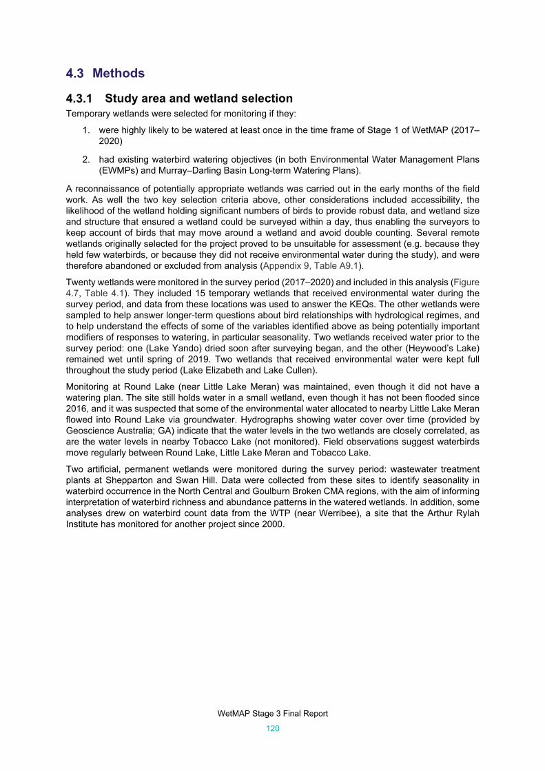
WetMAP Stage 3 Final Report
120
Methods
Study area and wetland selection Temporary wetlands were selected for monitoring if they:
1. were highly likely to be watered at least once in the time frame of Stage 1 of WetMAP (2017–2020)
2. had existing waterbird watering objectives (in both Environmental Water Management Plans (EWMPs) and Murray–Darling Basin Long-term Watering Plans).
A reconnaissance of potentially appropriate wetlands was carried out in the early months of the field work. As well the two key selection criteria above, other considerations included accessibility, the likelihood of the wetland holding significant numbers of birds to provide robust data, and wetland size and structure that ensured a wetland could be surveyed within a day, thus enabling the surveyors to keep account of birds that may move around a wetland and avoid double counting. Several remote wetlands originally selected for the project proved to be unsuitable for assessment (e.g. because they held few waterbirds, or because they did not receive environmental water during the study), and were therefore abandoned or excluded from analysis (Appendix 9, Table A9.1).
Twenty wetlands were monitored in the survey period (2017–2020) and included in this analysis (Figure 4.7, Table 4.1). They included 15 temporary wetlands that received environmental water during the survey period, and data from these locations was used to answer the KEQs. The other wetlands were sampled to help answer longer-term questions about bird relationships with hydrological regimes, and to help understand the effects of some of the variables identified above as being potentially important modifiers of responses to watering, in particular seasonality. Two wetlands received water prior to the survey period: one (Lake Yando) dried soon after surveying began, and the other (Heywood’s Lake) remained wet until spring of 2019. Two wetlands that received environmental water were kept full throughout the study period (Lake Elizabeth and Lake Cullen).
Monitoring at Round Lake (near Little Lake Meran) was maintained, even though it did not have a watering plan. The site still holds water in a small wetland, even though it has not been flooded since 2016, and it was suspected that some of the environmental water allocated to nearby Little Lake Meran flowed into Round Lake via groundwater. Hydrographs showing water cover over time (provided by Geoscience Australia; GA) indicate that the water levels in the two wetlands are closely correlated, as are the water levels in nearby Tobacco Lake (not monitored). Field observations suggest waterbirds move regularly between Round Lake, Little Lake Meran and Tobacco Lake.
Two artificial, permanent wetlands were monitored during the survey period: wastewater treatment plants at Shepparton and Swan Hill. Data were collected from these sites to identify seasonality in waterbird occurrence in the North Central and Goulburn Broken CMA regions, with the aim of informing interpretation of waterbird richness and abundance patterns in the watered wetlands. In addition, some analyses drew on waterbird count data from the WTP (near Werribee), a site that the Arthur Rylah Institute has monitored for another project since 2000.

WetMAP Stage 3 Final Report
121
Figure 4.7: Map of sites monitored for birds.
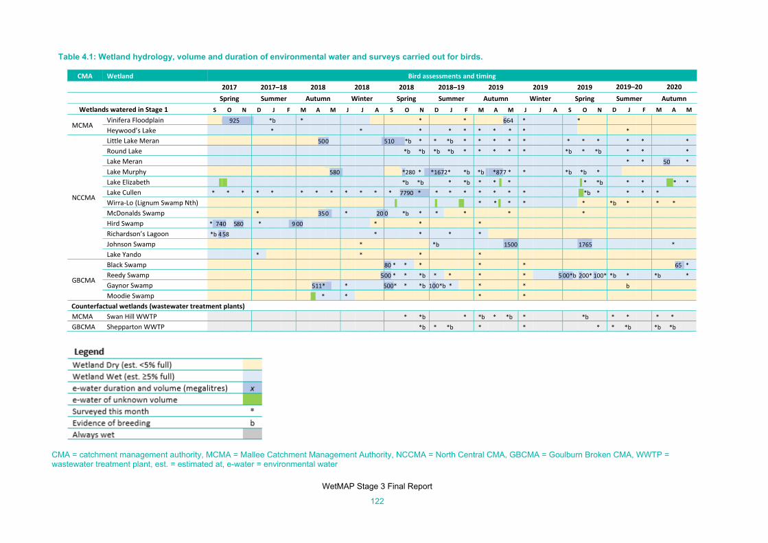
WetMAP Stage 3 Final Report
122
Table 4.1: Wetland hydrology, volume and duration of environmental water and surveys carried out for birds.
CMA = catchment management authority, MCMA = Mallee Catchment Management Authority, NCCMA = North Central CMA, GBCMA = Goulburn Broken CMA, WWTP = wastewater treatment plant, est. = estimated at, e-water = environmental water
CMA Wetland Bird assessments and timing 2017 2017–18 2018 2018 2018 2018–19 2019 2019 2019 2019–20 2020
Spring Summer Autumn Winter Spring Summer Autumn Winter Spring Summer Autumn Wetlands watered in Stage 1 S O N D J F M A M J J A S O N D J F M A M J J A S O N D J F M A M
MCMA Vinifera Floodplain eee925eeee! *b * * * 664 * *
Heywood’s Lake * * * * * * * * * *
NCCMA
Little Lake Meran 5000 |||||510||e *b * * *b * * * * * * * * * * *
Round Lake *b *b *b *b * * * * * *b * *b * * *
Lake Meran * * 50 *
Lake Murphy 580| *2800 * 1 *1672* *b *b || *8777 * * *b *b *
Lake Elizabeth | | *b *b * *b * * t * t * *b * * Tt|* *
Lake Cullen * * * * * * * * * * * * 7790| *||| * * * * * * * t *b * * * *
Wirra‐Lo (Lignum Swamp Nth) t t t* * * t * * * *b * * *
McDonalds Swamp * 3500| * 20 0 *b * * * * *
Hird Swamp *|7440| 580 * |9 00 * * *
Richardson’s Lagoon *b 4558 * * * *
Johnson Swamp * *b 1500 1765 *
Lake Yando * * * *
GBCMA
Black Swamp 80 * * * * * 65| *
Reedy Swamp |5|500 * * *b * * * * |500*b 200* 100* *b * *b *
Gaynor Swamp 511*|| * 500* * *b 100*bb * * * b
Moodie Swamp t * * * *
Counterfactual wetlands (wastewater treatment plants)
MCMA Swan Hill WWTP * *b * *b * *b * *b * * * *
GBCMA Shepparton WWTP *b * *b * * * * *b *b *b

WetMAP Stage 3 Final Report
123
Monitoring frequency and timing WetMAP bird monitoring surveys were adapted over the 3 years of field work. In 2017–2018, the aim was to conduct surveys once prior to watering and twice while inundated. Preliminary examination of the data indicated that more frequent surveys were required, given the high variability in waterbird counts. During 2018–2019, monthly surveys of each wetland were undertaken while they held water, then every 2 months once wetlands dried (Table 4.1). During the 2019–2020 survey season, regular survey periods were continued, but the survey interval was increased to 6 weeks which enabled more sites to be monitored. Once wetlands had dried out, the survey interval was reduced to once every 3 months or ceased, allowing resources to be focused on counts at wet sites.
The exact timing of field trips was occasionally altered, and a few field trips were cancelled, to avoid weather extremes (heavy rain, strong winds or high temperatures) that could reduce waterbird detectability or were incompatible with departmental OH&S practices.
Survey methods Waterbird surveys were conducted in daylight hours by two-person teams. The following waterbird measures were recorded at all wetlands:
a count of the number of each species seen on the wetland
evidence of breeding
the habitat type in which each bird species was observed
the percentage of species or species groups actively feeding within each habitat type.
Details of each of these are outlined below.
Waterbird counts All wetlands were surveyed using binoculars and tripod-mounted spotting scopes. Each survey aimed to obtain a consistent ‘complete count’, identifying and counting all visible waterbirds. At most wetlands, a complete count could be achieved from set vantage points. For wetlands at which selected vantage points did not allow adequate coverage of the site, consistent walking routes through the wetland were included to ensure that no corners of the wetland were missed and to walk through vegetated habitats and check whether birds were concealed in them (see examples in Figure 4.8). At Lake Murphy and Lake Cullen this involved walking around or through stands of Cumbungi (Typha sp.) and reeds (Phragmites sp.) in search of bitterns.
This survey technique is unlikely to detect all individuals of cryptic groups such as rails, crakes, bitterns and warblers. Therefore, counts of each species were classified as ‘complete’ or ‘partial’, according to observers’ perceptions of whether survey coverage was sufficient to detect all individuals. Typically, counts of large-bodied species (e.g. herons and spoonbills) and those waterbirds concentrated in sparsely vegetated parts of the wetlands (e.g. ducks and shorebirds) were considered complete, whereas counts of species that preferred denser vegetation [e.g. Little Grassbirds (Megalurus gramineous) and Reed Warblers (Acrocephalus australis), which were often only heard] were considered partial.
All observed birds were classified into feeding guilds, which were adapted from Loyn et al. (2014), Maher et al. (1991) and D. Roshier (unpublished). See Appendix 1 for further details of guild assignment. Guild definitions are provided in the introduction. Guilds were used as a way of simplifying the dataset, rather than having separate analyses for approximately 80 species. It was assumed that species within these guilds are likely to respond similarly to changes in water availability, and there is likely to be greater variability between the responses of different guilds than differing species.
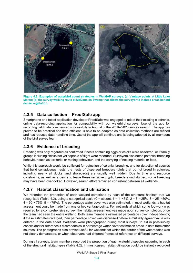
WetMAP Stage 3 Final Report
124
Figure 4.8: Examples of waterbird count strategies in WetMAP surveys. (a) Vantage points at Little Lake Meran; (b) the survey walking route at McDonalds Swamp that allows the surveyor to include areas behind dense vegetation.
Data collection – ProofSafe app Smartphone and tablet application developer ProofSafe was engaged to adapt their existing electronic, online data-recording application for compatibility with our waterbird surveys. Use of the app for recording field data commenced successfully in August of the 2019– 2020 survey season. The app has proven to be practical and time efficient, is able to be adapted as data collection methods are refined and has reduced data-handling time. Use of the app will continue and is being adopted by all members of the bird survey team.
Evidence of breeding Breeding was only regarded as confirmed if nests containing eggs or chicks were observed, or if family groups including chicks not yet capable of flight were recorded. Surveyors also noted potential breeding behaviour such as territorial or mating behaviour, and the carrying of nesting material or food.
While this approach would be sufficient for detection of colonial breeding, and for detection of species that build conspicuous nests, the nests of dispersed breeders (birds that do not breed in colonies, including nearly all ducks, and shorebirds) are usually well hidden. Due to time and resource constraints, as well as a desire to leave these sensitive cryptic breeders undisturbed, some breeding may have been overlooked. However, search effort remained consistent between all wetlands.
Habitat classification and utilisation We recorded the proportion of each wetland comprised by each of the structural habitats that we recognised (Table 4.2), using a categorical scale (0 = absent, 1 = 1–<5%, 2 = 5–<25%, 3 = 25–<50%, 4 = 50–<75%, 5 = >75%). The percentage water cover was also estimated. In most wetlands, a habitat assessment could be made from one or two vantage points. For wetlands at which some footwork was required for a comprehensive survey, the habitat assessment was made upon survey completion, once the team had seen the entire wetland. Both team members estimated percentage cover independently; if these estimates diverged, then percentage cover was discussed before a mutually agreed value was entered in the data sheet. Wetlands were photographed during most surveys, to aid in post-survey checks and for reference if discrepancies in percentage water cover estimation arose in data from other sources. The photographs also proved useful for wetlands for which the border of the waterbodies was not clearly demarcated, or when observers had different frames of reference on different surveys.
During all surveys, team members recorded the proportion of each waterbird species occurring in each of the structural habitat types (Table 4.2). In most cases, habitat utilisation could be instantly recorded

WetMAP Stage 3 Final Report
125
for each group of a species. For instances where birds were unsettled, moving between habitat types during the survey in response to disturbance, we recorded perceptions of the ‘average’ proportion of birds based on the habitat type in which they were originally seen. This was done to avoid skewing data with habitat use after disturbance.
Table 4.2: Structural habitat categories assessed at each wetland during surveys.
Woodland birds Woodland birds were assessed using an adapted version of the area search technique used by BirdLife Australia (BLA) for Atlas surveys (https://birdata.birdlife.org.au/survey-techniques). We used 10-minute counts conducted over a 1-ha area, rather than BLA’s 20-minute 2-ha surveys, because the woodland areas surrounding the study wetlands were often smaller than 2 ha. The extent of woodland around wetlands varied, allowing between 4 and 8 1-ha plots. The shape of each plot was also adjusted to match that of the available habitat (e.g. Figure 4.9). Woodland bird surveys were only carried out at 12 wetlands that were surrounded by woodland areas large enough to be monitored using this area search technique (Black Swamp, Gaynor Swamp, Heywood’s Lake, Lake Elizabeth, Lake Yando, Little Lake Meran, Moodie Swamp, Reedy Swamp, Richardson’s Lagoon, Round Lake, Vinifera Floodplain and Wirra-Lo (Lignum Swamp Nth)).
All woodland bird surveys were carried out in daylight hours, and we avoided carrying out the surveys in strong wind conditions or high temperatures >35o C. Time of day and weather conditions can influence the diversity and abundance of woodland birds recorded, though Ellis and Taylor (2018) show they do not have as large an effect as is often popularly assumed. The time of survey and weather conditions were recorded during WetMAP surveys; they did not differ systematically between wetlands with and without environmental water and were not eventually used in our assessment of whether woodland bird species richness and abundance differed between wetlands with and without water.
Habitat type Habitat code Surface water habitats Deep Open Water (not wadable for birds) DOW Shallow Open Water (waterbirds able to wade in it) SOW Shallow Water with Emergent Plants (e.g. reeds, rushes, sedges/grass, lignum, saltmarsh, trees)
SWE
Aquatic Vegetation (floating or submerged) AQV Wetland fringe habitats Bare Wet Substrate (mud or sand) BWS Bare Dry Substrate (dry mud or dry sand) BDS Shoreline Vegetation: No Bird Cover – too short to hide birds (e.g. close-cropped grass, some short/sparse saltmarsh)
NC
Shoreline Vegetation: Low Bird Cover – short to medium vegetation, tall enough to hide birds but < knee depth (grasses, sedges, salt marsh)
LC
Shoreline Vegetation: Tall Bird Cover – long vegetation TC Habitats throughout wetland (both in surface water and on fringes) Lignum L Tall Marsh (Typha sp./Phragmites sp.) TM Black Box BB River Red Gum RG Unidentified Stags US Other Substrate (for nesting purpose – please state) OS

WetMAP Stage 3 Final Report
126
Figure 4.9: Woodland bird count sites, Moodie Swamp (GBCMA). 1-ha surveyed areas vary in shape, dependent on the fringing vegetation.
Water quality and zooplankton Water quality was measured using a YSI ProDSS portable water quality multiparameter (Xylem Analytics Australia). At most wetlands, water quality parameters were measured at a depth of at least 10 cm beneath the water surface at two locations – one location on the windward side and one location on the leeward side of the wetland (based on conditions on the day that the wetland was surveyed). The aim was to detect any difference there might be in water quality due to wind movement and hence any influence this may have on waterbird distribution within the wetland. Disturbance of aquatic vegetation and substrate was avoided to ensure measurements were taken in water conditions that could be considered normal for that wetland at the time of the survey. If water levels were low, the instrument was laid on its side to submerge all probes, and any turbidity within the water caused by the approach of the observers was allowed to settle before readings were taken. Location (as shown by handheld GPS) and time at which each sample was taken was recorded.
Water quality parameters measured were:
water temperature pH electrical conductivity dissolved oxygen concentration.
Water quality data were collected to support analyses for the longer-term WetMAP KEQs and SQs, and are therefore not discussed further in this report.
Zooplankton samples were collected to provide a simple measure of wetland productivity, to test for a correlation with waterbird food abundance. The long-term intention is to assess lag times between water delivery, zooplankton abundance and waterbird responses. This data will support future analyses and is also not discussed further in this report.
WetMAP Stage 3 Final Report
127
Hydrological history Hydrological data were sourced from Geoscience Australia (https://www.ga.gov.au/) to aid in a preliminary evaluation of the longer-term KEQs and SQs. Time series data of water extent allowed us to examine the relationship between bird numbers and hydrological patterns. We used several hydrological predictors related to proportion of a wetland that was wet, duration of inundation, and time since the wetland was dry. More detail about these predictors is provided in Appendix 3.
Statistical analysis Our statistical analysis had three main goals:
1. to answer the four KEQs, which collectively examine whether environmental watering is beneficial for birds at our focal wetlands (KEQs 1–4)
2. to relate bird response variables to a range of hydrological predictors, to begin exploring relationships between bird response and hydrological regimes (SQ1–SQ3)
3. to explore the influence of water availability across the Australian landscape on bird numbers in Victoria (SQ4).
KEQ 1: Do environmental water events increase the abundance and species richness of birds in wetlands? We compared the number and species richness of birds (all waterbirds, and within guilds) observed during wet and dry hydrological phases at 12 wetlands in which both wet and dry phases occurred (‘dry’ being defined as ≤5% total water, ‘wet’ >5% total water). In total, data were available from 74 surveys carried out when wetlands were ‘wet” and from 30 surveys carried out when the same wetlands were dry. We tested whether the number and richness of waterbirds differed between hydrological phases using generalised linear mixed-effects models, which were run using the glmer function in the lme4 package in R.
Our first two analyses tested whether the species richness and counts of all waterbirds differed between hydrological phases (two levels, wet or dry) and seasons (four levels), and whether potential differences between hydrological phases were consistent or not between seasons (i.e. hydrological phase*season interaction). This model therefore included hydrological phase and season as fixed effects, and wetland and year as random effects. These two models were both fitted (after log-transforming response variables) using a Gaussian distribution. Counts of Large Waders were skewed after both log- and square-root transformation, so we fitted a negative binomial model (using the glmer.nb function); a full model (hydrological phase and season as fixed effects; wetland and year as random) would not converge, so season was excluded. The counts of four guilds (Shallow Waterfowl, Skulkers, Shorebirds and Swimming Piscivores) were highly skewed, with many small or zero values, and a small number of very large counts (i.e. thousands of birds). For these guilds, we tested whether the probability of occurrence differed between hydrological phases using a binomial generalised linear mixed model with year and wetland as random factors, as above. These models would also not converge with season as a fixed effect, so season was removed. We present the results for each binomial model, together with summaries of the data (i.e. counts) to help interpretation. We assessed all models by examining residual and Q–Q plots, and evaluated overdispersion using the dispersion.glmer function from the blmeco package. Predictions for fixed effects (adjusted for random effects) were extracted using functions in the emmeans package and are presented after being back-transformed to the scale of the response.
KEQ 2. Do environmental water events result in bird breeding at wetlands? There were few breeding records, and there were insufficient data for statistical analysis. Instead, we present summaries of breeding observations.

WetMAP Stage 3 Final Report
128
KEQ 3. Do environmental water events increase suitable habitat for foraging, roosting and breeding of waterbirds in wetlands? To answer this question, we first used graphical approaches and tabulation to examine the extent to which a selection of bird species across the various guilds used the habitat types that we predicted would be important for them.
We then tested whether the availability of eight habitat types identified as being used by various bird species changed following environmental flows. To do so, we used data from the 12 wetlands that had both a wet and a dry hydrological phase, consistent with KEQ 1. We assessed whether the probability of each habitat variable being given a habitat score of between 0 (i.e. 0%) and 5 (i.e. 75–100%) was consistent between wet and dry hydrological phases. For this, we used ordinal mixed-effects regression models, which were implemented using the clmm function from the ordinal package in R. For each habitat variable, we ran a model that included hydrological phase (two levels: wet or dry) as a fixed effect (models with season included did not converge); wetland and year were included as random effects. Model predictions were extracted using the ggpredict function from the ggeffects package.
We also examined whether the availability of these eight habitat types was related to the level of water in wetlands. To do so, we examined the relationship between the probability of a habitat variable being given a score of between 0 and 5, and the proportion of the wetland holding water (hereafter ‘wet proportion’). This model followed the methods above, but ‘Wet proportion’ was included as a continuous predictor, rather than the categorical hydrological phase. We also included data from all wetlands sampled in the bird theme, to explore these relationships across a wider range of sites.
KEQ 4. Do environmental water events increase the abundance and species richness of woodland birds adjacent to wetlands? We compared the number and species richness of all woodland birds observed during wet and dry hydrological phases at the 12 wetlands at which both wet and dry phases occurred during the study. To do so, we used Wilcoxon signed-rank tests.
To explore the relationship between woodland bird abundance and richness and water availability in the adjacent wetland, we also graphed these variables against the wet proportion. These figures included data from all wetlands (i.e. not just those that had both wet and dry hydrological phases).
SQs 1–3: Exploration of bird relationships with hydrological regimes We selected hydrological predictors that describe the axes in our response curve conceptual models (Section 4.1.3; Figures 4.11, 4.12 and 4.13), that is, the key hydrological gradients to which birds might respond. Detailed depth data from all wetlands is not yet available, so we assumed that wet proportion was an adequate proxy for depth (an assumption that needs to be tested in the future). Water availability time series were provided by GA from their Wetland Insights Tool. The selection of predictors with justification is outlined in Table 4.3.
Table 4.3: Selection of predictors for analysis.
Predictor Relation to hydrological phase Justification/link to conceptual model
Proportion of the wetland that was wet (hereafter ‘wet proportion’)
Water extent, likely proxy for depth and duration/frequency of inundation
Short-term (i.e. 1–6 months) changes in water level could relate to potential changes in habitat availability, e.g. breeding sites or food resources.
Proportion of the wetland that was wet in antecedent periods ranging from 1 month to 1 year [hereafter ‘wet proportion (with antecedent period)’]
Water extent likely proxy for depth and duration/frequency of inundation
Annual changes in water level could relate to other habitat aspects that respond over long-term scales, e.g. extent of Tall Marsh habitat.
Time wetland has held water (with dry samples set as zero)
Duration of flooding Wetlands need to hold water for sufficient periods for food resources to develop, but if wet for too long some habitat elements may be overgrown by dense fringing vegetation.

WetMAP Stage 3 Final Report
129
We ran a series of analyses to explore the potential influence of wetland hydrology and size on bird responses (the latter being included because larger wetlands may attract more birds, regardless of hydrological characteristics). We used the following response variables: total number of all birds (including terrestrial species), total number of waterbirds, and numbers of the species that numerically dominate each of the four commonest guilds [Shorebirds: Black-winged Stilt (Himantopus himantopus); Shallow Waterfowl: Grey Teal (Anas gracilis); Deep Waterfowl: Black Swan; Swimming Piscivores: Hoary-headed Grebe (Poliocephalus poliocephalus)]. We ultimately did not conduct analyses for Grey Teal though, as their numbers were highly correlated with total waterbird numbers (r > 0.7). We did not use species richness as a response variable because it was highly correlated with total numbers of waterbirds (linear mixed-effects model with wetland and year as random effects: Chi-square = 793.05, df = 1, p < 0.001). Total number was used over species richness because conservation targets are often developed for the total number of birds (e.g. Ramsar Convention criteria 5 and 6 for the recognition of internationally significant wetlands are based on numbers of waterbirds; there are no specific Ramsar criteria for species richness; Department of Agriculture, Water and the Environment 2020).
We related numbers of each response variable to the following predictors: wetland size, wet proportion on day of sampling, average daily wet proportion over four antecedent periods (30, 90, 180 and 360 days), and time since wetland had dried. We also considered whether relationships between birds and these predictors varied among seasons. We removed the three wastewater treatment plants from these analyses, because these wetlands have other characteristics that are likely to confound our ability to interpret hydrological effects (e.g. high nutrients and presumably high food abundance).
For the total number of birds and number of waterbirds, we fitted a generalised additive model (GAM) with the gamm4 function from the mgcv package, using a negative binomial distribution, with wetland and year included as random effects. We fitted a model for each predictor individually and a null (intercept-only) model, and then selected the best-fitting model based on the Akaike Information Criteria corrected for small sample sizes (AICc). Our data were sufficient to then run further models with the two best individual predictors, and with Season as a categorical predictor to test whether relationships were consistent across seasons. These models were evaluated using the gam.check and dispersion_glmer functions.
Responses for numbers of individual species had a very high (>40%) proportion of zero counts. For these responses, we fitted zero-inflated binomial mixed models (year and wetland as random effects) using functions in the glmmTMB package. As above, we combined the two best predictors into a more complex model. Model selection was undertaken using AICc as above, including a null (intercept-only) model as above. Residuals and Q–Q plots were examined for all models. Model predictors were extracted for all models.
SQ 4: Are waterbird abundance and species diversity affected by continental rainfall patterns and water availability in the Australian landscape? To examine the potential influence of water availability in the Australian landscape on the numbers of birds in Victorian wetlands, we used data from the WTP as a case study. We had hoped to use waterbird count data from wetlands within the North Central or Goulburn Broken CMAs, where most of our WetMAP sites are located. However, while waterbirds have been counted in many wetlands, few long-term datasets are available, and we were unable to find any single wetland with a sufficiently long time series (>15 years) to support these analyses; in comparison, the WTP has been monitored intensively since 2000. We therefore present these analyses as an initial ‘proof of concept’ exercise and discuss later in the report some options for gathering a longer-term dataset from areas more representative of the WetMAP sites in the future.
Water availability data We initially examined water availability for 30 wetland complexes identified as being key habitats for birds in the Murray–Darling Basin (https://www.ga.gov.au/__data/assets/pdf_file/0017/90143/DEA-Program-Roadmap-Dec2019.pdf), in addition to the Western District Lakes in Victoria. Water availability time series were provided by GA. We calculated an annual measure of water availability (1 July – 30 June, which is often used as a hydrological year, and matches our methodology for bird counts, see below) as the sum of the two wettest categories (‘wofs_area_percent’ and ‘tcw_area_percent’) across

WetMAP Stage 3 Final Report
130
the year. The 30 wetland complexes are located within 12 of the river basin regions as defined in the GA 1997 River Basins network layer (http://www.bom.gov.au/water/about/image/basin-hi_grid.jpg).
Our primary interest was in assessing the relationship between bird numbers at the WTP and water availability at large spatial scales, not in identifying particular individual wetland complexes that birds used. We also anticipated that nearby locations (e.g. in the same drainage areas) would likely be correlated in terms of annual changes in water availability. We therefore aggregated data from each of these complexes to calculate a region-level estimate of water availability. We did this by taking the average annual measure of wetness across all wetland complexes in each region multiplied by the size of the region for which water availability had been assessed (in square kilometres). We used the area of the region rather than wetland area because we were concerned using the latter would mean we did not capture all available habitat. After this process, we were left with 10 water availability regions: Condamine, Goulburn–Loddon, Lachlan–Murrumbidgee, Lower Murray, Macquarie, Menindee Lakes, Namoi–Gwydir, Warrego, Wimmera–Mallee and the Western District Lakes.
We then further aggregated data from regions that were highly correlated (Pearson’s r > 0.75) into the following groups (Figure 4.10):
1. Goulburn–Loddon, Lachlan–Murrumbidgee, Wimmera–Mallee (hereafter GL_LM_WM)
2. Condamine, Menindee Lakes, Warrego (COND_ML_WAR)
3. Lower Murray and Coorong (LOWER_MURRAY)
4. Namoi–Gwydir (NAMOI_GWYDIR)
5. Macquarie Marshes (MACQUARIE)
6. Western District Lakes (WDL).
Finally, we examined correlations (Pearson’s r) between these regions. The GL_LM_WM region was highly correlated with the MACQUARIE, COND_ML_WAR, and WDL (Pearson’s r 0.81–0.97, Appendix 11, Table A11.1). We therefore selected GL_LM_WM, LOWER_MURRAY and NAMOI__GWYDIR as our predictor variables.

WetMAP Stage 3 Final Report
131
Figure 4.10. Wetland complexes for which water cover was compared with waterbird numbers at the WTP.
Western Treatment Plant bird counts We obtained annual bird counts for the WTP from long-term monitoring programs that have been undertaken by ARI every year for the period 2000–2020 (Loyn et al. 2014; ARI unpublished data). During this program, the WTP has been sampled approximately every 2 months in most years (although counts have been reduced to three per year more recently), with each sampling ‘session’ lasting multiple days. We took the average of the maximum counts recorded over the austral summer (November to February) for each year from 2000 to 2018, based on fiscal years (i.e. 1 July – 30 June), so all counts for each austral summer were included in one year.
The WTP is largely used by waterbirds as a non-breeding area; few waterbird species breed there. We therefore hypothesised that waterbird numbers would be lowest at the WTP at times when the abundance of alternate habitat elsewhere (especially breeding habitat) was most extensive.
We selected nine focal species that spanned five bird guilds that we hypothesised may respond in different ways to water availability elsewhere (Table 4.4). We did not include a representative from the Skulkers or Large Waders guilds, because we did not have sufficient counts of these species to warrant statistical analysis.

WetMAP Stage 3 Final Report
132
Table 4.4: Focal bird species used in the analysis of responses of waterbirds to availability of wetland habitats in different regions of eastern Australia.
Common name Guild Predicted response
Pink-eared Duck (Malacorhynchus membranaceus)
Shallow Waterfowl
Widespread throughout inland Australia. Numbers at the WTP often peak in early rather than late summer, so we hypothesised WTP numbers might be negatively correlated with wetlands far inland, which dry earlier, and might receive some monsoonal rain in late summer to autumn.
Freckled Duck (Stictonetta naevosa)
Shallow Waterfowl
Has a strong preference for nesting in lignum, and Victorian counts are modest compared with those in New South Wales; we therefore hypothesised that abundance may be most strongly related to water availability in the largest areas of lignum in wetlands of northern New South Wales.
Grey Teal (Anas gracilis)
Shallow Waterfowl
Summer peaks at WTP; very widespread throughout inland Australia. Seasonal occurrence at the WTP very similar to that of Hoary-headed Grebe and Eurasian Coot, so we anticipated a similar response to inland water availability in all three.
Chestnut Teal (Anas castanea)
Shallow Waterfowl
Largely confined to southern Australia, so we hypothesised that it would respond more strongly to water availability in southern regions, and less strongly to water availability in Queensland or northern New South Wales.
Eurasian Coot (Fulica atra)
Deep Waterfowl
Summer peaks at WTP; widespread throughout inland Australia. Seasonal occurrence at the WTP very similar to that of Hoary-headed Grebe and Grey Teal, so we anticipated a similar response to inland water availability in all three.
Australian Shelduck (Tadorna tadornoides)
Shallow Waterfowl
Largely confined to southern Australia, so we hypothesised that it would respond more strongly to water availability in southern regions, and less strongly to water availability in Queensland or northern New South Wales.
Hoary-headed Grebe (Poliocephalus poliocephalus)
Swimming Piscivores
Summer peaks at WTP; very widespread throughout inland Australia. Seasonal occurrence at the WTP very similar to that of Grey Teal and Eurasian Coot, so we anticipated a similar response to inland water availability in all three.
Blue-billed Duck (Oxyura australis)
Deep Waterfowl
WTP numbers peak in early winter rather than summer, suggesting use of different breeding areas from most other species considered here. We were unsure what response to expect but thought it may differ from other species.
Black-winged Stilt (Himantopus himantopus)
Shorebirds Summer peaks at WTP; widespread throughout inland Australia. We anticipated the strongest inverse relationship between WTP counts and water availability in more southern drainage basins, reasoning that birds retreating from drought in more northerly inland wetlands would probably evacuate to more northerly drought refuges (e.g. in the wet–dry tropics).
Sharp-tailed Sandpiper (Calidris acuminata)
Shorebirds Summer peaks at WTP; widespread throughout inland Australia. We anticipated the strongest inverse relationship between WTP counts and water availability in more southern drainage basins, reasoning that birds retreating from drought in more northerly inland wetlands would probably evacuate to more northerly drought refuges (e.g. in the wet–dry tropics) as this would reduce the distance of their annual northward migration to Siberia.

WetMAP Stage 3 Final Report
133
Modelling We compared relationships between annual bird counts at the WTP with annual measures of water availability from the three focal areas using generalised additive models (GAMs), which were fitted using the gamm4 package in R. For each species, we initially ran two models: (1) a null model with the intercept only, and (2) a model with Year, to test for an annual trend. We compared the fit of these models using Akaike Information Criteria corrected for small sample sizes (AICc) and selected the best-fitting one to act as our model for comparison.
We then ran a separate model relating bird counts to water availability at each location, including year where it was in the best comparison model, or the null (intercept-only) model if not. We had complete datasets for GLMM_LW_MW and NAMOI_GWYDIR, with estimates of water availability for all years. We therefore compared models for these two locations with the best comparison model based on AICc using the model.sel function from the MuMin package, and present these along with the p-values for the location smoother, and also the year (where this was the best comparison model). There were several years with missing data from the LOWER_MURRAY, that is, when no estimates of water availability were available, so we could not directly compare the fit of models using the LOWER_MURRAY and the other two locations. For the LOWER_MURRAY, we therefore just tested the significance of models based on the p-value for the smoother rather than AICc. We evaluated all models using the gam.check function and, where necessary, transformed the predictor and/or response variables to normalise the data and reduce heteroscedasticity as much as possible. For influential predictor variables (i.e. in the best models, with p-values < 0.05), we extracted and plotted predictions.
Results We focus our presentation of results on answering the Key Evaluation and SQs outlined in the Introduction. Broad summaries of the bird-monitoring results (e.g. species lists and counts) are provided in Appendix 9.
KEQ 1: Do environmental water events increase the abundance and species richness of birds in wetlands?
Environmental water events resulted in higher species richness and abundance during the wet hydrological phases.
The number of waterbird species and total abundances of all waterbirds was higher in samples taken during the wet hydrological phase (Figure 4.11a and b; Table 4.5), and this pattern was consistent across seasons (i.e. no ‘Hydrological phase * Season’ interaction in Table 4.5). While the analysis was based on comparing overall patterns, summaries of the data show that both waterbird richness and abundance were higher at all sites in the wet hydrological phases (Figure 4.12). However, the response was most pronounced at several sites where no birds were observed during dry periods (e.g. Gaynor Swamp, Hird Swamp West, Heywood’s Lake, Lake Murphy and Reedy Swamp).
The number of Large Waders was significantly higher in the wet phase (Figure 4.11c, Table 4.5). The probability of observing Shallow Waterfowl, Skulkers, Shorebirds and Swimming Piscivores differed between hydrological phases (Table 4.5). There were only two surveys of dry sites on which more than 20 Shallow Waterfowl were observed (maximum count of 231). In comparison the number of shallow waterfowl exceeded 20 on 61 of the 74 surveys carried out when wetlands held water (maximum count 9074). More than 35 Skulkers were observed on only two occasions, both in the wet phase, and all four counts of more than 40 Shorebirds also occurred in the wet phase. While the data were too sparse to statistically test whether numbers of the three remaining guilds varied between wet and dry phases, there were more observations of all guilds from wet samples (Shorebirds: 38 observations, 37 in wet; Deep Waterfowl: 16 observations, total of 385 birds, all in wet; Terns: 6 observations, total of 3030 birds, all in wet).

WetMAP Stage 3 Final Report
134
Figure 4.11: Predicted values from generalised linear mixed-effects models comparing bird responses in dry (≤5% total water) and wet (>5% water) hydrological phases. For species richness and total numbers of birds, sufficient data were available to also include season as a fixed effect in these models. Symbols show mean prediction, and error bars the 95% confidence interval.

WetMAP Stage 3 Final Report
135
Legend BLSW Black Swamp GASW Gaynor Swamp HISW_EAST Hird Swamp East HISW_WEST Hird Swamp West LAHE Lake Heywood LAMU_NORTH Lake Murphy North LAMU_SOUTH Lake Murphy South MCSW McDonalds Swamp RESW Reedy Swamp RILA_WEST Richardson’s Lagoon West VINI Vinifera Floodplain WILO_LS Wirra-Lo (Lignum Swamp North)
Figure 4.12: Waterbird richness at 12 sites that were sampled during both dry and wet hydrological phases. Table 4.5: Analysis of deviance table comparing bird responses in dry and wet hydrological phases.
Hydrological phase Season Hydrological phase*Season
Variable Chi-sq (all 1 df)
p Chi-sq (all 3 df)
p Chi-sq (all 3 df)
p
Waterbirds (richness) 106.9 <0.001 7.83 0.05 0.91 0.71
Waterbirds (abundance) 89.07 <0.001 7.84 <0.05 0.76 0.86
Large Waders (abundance) 2.42 <0.001
Shallow Waterfowl (presence) 26.87 <0.001
Skulkers (presence) 7.79 <0.001
Shorebirds (presence) 2.71 <0.001
Swimming Piscivores (presence) 3.96 <0.001

WetMAP Stage 3 Final Report
136
KEQ2: Do environmental water events result in bird breeding at wetlands?
While breeding was relatively rare, the majority of records were from wetlands that received environmental water. In total, we made 117 confirmed observations of breeding attempts across 14 species of waterbirds across all sites (Table 4.6), with 102 of these records (across 12 species) from wetlands that received environmental water. Many of these breeding attempts included clutches of several eggs or broods of several young. The majority of breeding observations (95%) were made from September to January; there were few breeding records in autumn or winter.
A large proportion of the breeding records involved a small number of species at a small number of sites. More than half of the breeding observations came from a single species, Black Swan, which nested colonially in Murphy Swamp in 2019; in addition, a mixed colony of Australasian Darter (Anhinga novaehollandiae) and Little Pied Cormorant (Microcarbo melanoleucos) nested at Johnson Swamp in 2019. There may also have been loose colonial nesting of Australasian Grebe (Tachybaptus novaehollandiae) at Round Lake; only four breeding records were confirmed at this site, but up to 20 pairs appeared to be nesting on floating vegetation in deep water; a boat would have been required to check whether these nests contained eggs.
The remaining breeding records involved dispersed nesting events. There were several observations of breeding by species that are listed as threatened or near-threatened: a pair of Brolga (Grus rubicunda) raised a chick, and a brood of 11 Australasian Shoveler (Anas rhynchotis) was observed at Lake Murphy in 2019. A single incubated nest of the (often colonial) Eastern Great Egret (Ardea modesta) was found at Round Lake in 2018, and broods of 6–7 Blue-billed Duck were observed at Swan Hill Wastewater Treatment Plant in both 2018 and 2019.
Behavioural observations (territorial behaviour, carrying of nesting material, entry into hollows and carrying of food) strongly suggested that a number of species were nesting in hollows of stags within wetlands. These species were Little and Long-billed Corella (Cacatua sanguinea and C. tenuirostris, respectively), Red-rumped Parrot (Psephotus haematonotus), Crimson and Eastern Rosellas (Platycercus elegans and P. eximius, respectively) and Striated Pardalote (Pardalotus striatus). In addition, a pair of Wedge-tailed Eagles (Aquila audax) nested at Johnson Swamp, and observations of dependent juveniles with their foraging parents suggested that the Vulnerable White-bellied Sea-Eagle (Haliaeetus leucogaster) nested near Gaynor Swamp, Lake Cullen, Lake Murphy, Heywood’s Lake, Reedy Swamp and Richardson’s Lagoon.

WetMAP Stage 3 Final Report
137
Table 4.6: Observations of confirmed breeding (eggs or flightless young) by site. Sites denoted with an asterisk* received environmental water during the study.
Site Australasian G
rebe
Australasian S
hoveler
Australian S
helduck
Black S
wan
Blue-billed D
uck
Brolg
a
Chestn
ut Teal
Australasian D
arter
Great E
gret
Grey T
eal
Little Pie
d Corm
orant
Masked L
apwing
Pacific B
lack Duck
White-faced H
eron
Grand T
otal
Black Swamp 0
Crow Swamp 1 1
Gaynor Swamp* 0
Heywood’s Lake 0
Hird Swamp* 0
Johnson Swamp* 2 14 1 17
Lake Cullen* 1 1
Lake Elizabeth* 1 1
Lake Murphy* 1 2 53 2 58
Lake Yando 0
Little Lake Meran* 1 1 1 3
McDonalds Swamp* 1 2 3
Moodie Swamp 0
Reedy Swamp (Shepparton)* 3 2 3 8
Richardson’s Lagoon* 2 1 3
Round Lake 4 1 1 1 7
Shepparton WWTP 1 1 1 5 8
Swan Hill WWTP 1 3 1 2 7
Vinifera Floodplain* 0
Wirra-Lo* 0
Grand total 5 1 8 59 3 2 1 3 1 4 14 1 14 1 117
WWTP = wastewater treatment plant
KEQ 3. Do environmental water events increase suitable habitat for foraging, roosting and breeding of waterbirds in wetlands?
A broad summary of habitat usage by different foraging guilds in WetMAP wetlands is provided in Appendix 10. Several habitat types were used extensively by different waterbird species, especially Deep Open Water and Shallow Open Water, and Bare Wet Substrate (Figure 4.13a). Habitat associations also varied by different guilds and species. For example, Deep Waterfowl are commonly observed in Deep Open Water habitat, while Large Waders; Shorebirds, Shallow Waterfowl and Terns made more use of Shallow Open Water. Shorebirds also tended to use Bare Wet Substrate. Heavily vegetated habitats at the fringes of wetlands (FLC, FTC and TM) were only preferred by a few skulking species (e.g. Purple Swamphen) and were avoided by shorebirds and ducks; shorebirds were also intolerant of dense emergent vegetation in shallow water.
At least visually, our data suggest many species used a narrower range of habitats when foraging (Figure 4.13b) than they did overall (Figure 4.13a). Birds that were not foraging when observed may

WetMAP Stage 3 Final Report
138
Figure 4.13: Proportion of selected species using different structural habitats in watered wetlands: (a) all waterbirds; (b) waterbirds observed while foraging.
Habitat types (x-axis) DOW Deep Open Water SOW Shallow Open Water AV Aquatic Vegetation WSE Water with Sparse Emergent veg. WMDE Water with Medium to Dense Emergent veg. BWS Bare Wet Substrate BDS Bare Dry Substrate FTC Fringing Tall Cover FBG Fringing Bare Ground TM Tall Marsh L Lignum SRG Stags and River River Red Gums U Unknown Guilds (right-hand axis) DWF Deep Waterfowl LWA Large Waders Shorebirds SK Skulkers SWF Shallow Waterfowl T Terns
(a)
(b)

WetMAP Stage 3 Final Report
139
have been carrying out other necessary maintenance behaviour (e.g. roosting, resting, preening) but it is also possible they included birds that had stopped foraging because they were aware of the presence of observers. While this does raise the possibility that habitat selection might have been influenced by the response of birds to disturbance (potentially from the observers in some cases), both potential data treatments indicated different habitat preferences by different guilds or species.
We found that environmental watering increased the availability of most habitats used by waterbirds (Figure 4.14). In some cases, these changes were very obvious. For example, Deep Open Water and Shallow Open Water were most often scored as a zero during the dry phase (i.e. reflecting 0% cover), but were scored as being between 1 and 4 approximately 80% of the time in the wet (Figure 4.14a and b). It is important to note that the 5% threshold we used to distinguish wet and dry samples is likely the reason why Deep and Shallow Open Water were not always scored as zero; in the final stages of drying out, for example, a wetland can hold less than 5% water cover, but the remaining water may lie in a puddle or pool that would be classified as Shallow Open Water or Deep Open Water. Both habitats are absent at completely dry wetlands. However, just because a wetland is watered doesn’t guarantee that all habitats will be present; hence, there is greater interest in the results for other variables. For example, there may be variability in the cover of Aquatic Vegetation even at wetlands with comparable levels of water. We also found higher cover of Shallow Water with Emergent Plants, Bare Wet Substrate, Aquatic Vegetation and Bare Dry Substrate in the wet hydrological phases (Figure 4.14). Cover of River Red Gum and Tall Marsh was generally scored as 1 (i.e. 1–20%) regardless of hydrological phase (Figure 4.14g and h). Above-ground perennial vegetation is unlikely to change by the >20% required to receive a different score on the 1–5 scale. The cover of many habitat variables was also related to the wet proportion of the day of sampling (Figure 4.15). As above, some of these results are obvious, but are presented for completeness. For example, the probability of observing no Deep Open Water was 80–100% when wetlands had no water, and the probability of Deep Open Water being >80% was 75% when wet proportion was 100% (Figure 4.15a). A similar trend was observed for Shallow Open Water (Figure 4.15a and b). More interesting results include higher cover of Shallow Water with Emergent Plants and Aquatic Vegetation increasing as the wet proportion increased (Figure 4.15c and e). River Red Gums and Tall Marshes were almost always scored as 0 or 1, with no relationships with wet proportion (Figure 4.15g and h).
Figure 4.14: Predictions from mixed-effects ordinal regression models showing the probability of observing particular cover scores for habitat variables during wet and dry phases.
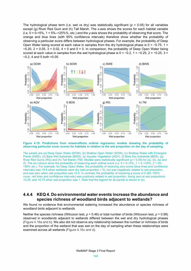
WetMAP Stage 3 Final Report
140
The hydrological phase term (i.e. wet vs dry) was statistically significant (p < 0.05) for all variables except (g) River Red Gum and (h) Tall Marsh. The x-axis shows the scores for each habitat variable (i.e. 0 = 0-<5%, 1 = 5%–<25%%, etc.) and the y-axis shows the probability of observing that score. The orange and blue lines (with 95% confidence intervals) therefore show whether the probability of observing a particular score differs between hydrological phases. For example, the probability of Deep Open Water being scored at each value in samples from the dry hydrological phase is 0 = ~0.75, 1 = ~0.20, 2 = 0.05, 3 = 0.02, 4 = 0 and 5 = 0. In comparison, the probability of Deep Open Water being scored at each value in samples from the wet hydrological phase is 0 = ~0.2, 1 = ~0.25, 2 = ~0.25, 3 = ~0.2, 4 and 5 both <0.05.
Figure 4.15: Predictions from mixed-effects ordinal regression models showing the probability of observing particular cover scores for habitats in relation to the wet proportion on the day of sampling. The panels are (a) Deep Open Water (DOW), (b) Shallow Open Water (SOW), (c) Shallow Water with Emergent Plants (SWE), (d) Bare Wet Substrate (BWS), (e) Aquatic Vegetation (AQV), (f) Bare Dry Substrate (BDS), (g) River Red Gums (RG) and (h) Tall Marsh (TM). Models were statistically significant (p < 0.05) for (a), (b), (e) and (f). The six colours show the probability of observing each ordinal score (i.e. 0 = 0-<5%, 1 = 5–>25%, 2 = 25–<50% etc.). For example, for Deep Open Water, the probability of receiving zero score (blue lines and confidence intervals) was >0.8 when wetlands were dry (wet proportion = 0), but was negatively related to wet proportion, and was zero when wet proportion was >0.5. In contrast, the probability of receiving a score of 5 (80–100% cover, red lines and confidence intervals) was positively related to wet proportion, being zero at wet proportions <0.25, and >0.75 when wet proportion was 1. Note that the legend for all panels is shown in (b).
KEQ 4. Do environmental water events increase the abundance and species richness of woodland birds adjacent to wetlands?
We found no evidence that environmental watering increased the abundance or species richness of woodland birds adjacent to wetlands
Neither the species richness (Wilcoxon test, p = 0.46) or total number of birds (Wilcoxon test, p = 0.99) observed in woodlands adjacent to wetlands differed between the wet and dry hydrological phases (Figure 4.16a and b). We also did not observe any relationship between the number or richness of birds and the proportion of the wetland that was wet on the day of sampling when these relationships were examined across all wetlands (Figure 4.16c and d).

WetMAP Stage 3 Final Report
141
Figure 4.16: Birds in the woodlands adjacent to wetlands during dry and wet hydrological phases in terms of (a) species richness and (b) abundance, and (c) species richness and (d) number of birds observed in woodlands in relation to the proportion of wetlands wet on the day of sampling. Note that for (a) and (b) only wetlands with wet and dry phases were included, while for (c) and (d) all wetlands were included.
SQ1–SQ3 Exploration of bird relationships with hydrological regimes
We found that several bird response variables were correlated with hydrological variables and wetland area (see model selection results in Appendix 10, Tables A10.2–A10.6). The total number of birds in wetlands (including both waterbirds and terrestrial species) was highest when wetlands were >80% wet in the past 30 days [wet proportion (30 days)], and at larger wetlands (Figure 4.17a). The number of waterbirds was best predicted by the proportion of the wetland that been wet for the past 90 days [wet proportion (90 days], with a positive relationship up until wet proportion (90 days) = ~0.8, and then there was some evidence of a plateau (Figure 4.17b). The number of Black-winged Stilts was very low when the wet proportion (30 days) was below 0.75 (Figure 4.17c). The number of Black Swans was very low when the wet proportion (90 days) was below 0.75 and increased thereafter, and there was some evidence that this relationship was more pronounced at larger wetlands (Figure 4.17d). Number of Hoary-headed Grebes was best predicted by wet proportion on the day of sampling (Figure 4.17e). In all instances, the relationships we detected did not vary by season (i.e. season was not in the best model for any species: Appendix 11, Table A11.2).

WetMAP Stage 3 Final Report
142
Figure 4.17: Predictions for models examining relationships between birds, hydrological predictors and wetland area. (a) Predictions from generalised additive mixed model relating the number of all birds to wetland area and the wet proportion (30 days); (b) predicted relationship between number of waterbirds and wet proportion (90 days) from generalised additive mixed model; (c) predicted relationship between number of Black-winged Stilts and wet proportion (30 days), from a zero-inflated negative binomial model; (d) relationship between the number of Black Swans and the wet proportion predicted from zero-inflated negative binomial models for six different area groups (shown in colours, units are hectares); (e) predicted relationship between the number of Hoary-headed Grebes and the wet proportion from zero-inflated negative binomial models. Note that mean predictions only are shown for panels (a) and (d). These panels show the best predictor for each response variable (see model selection results in Appendix 10, Tables A10.2–A10.6).

WetMAP Stage 3 Final Report
143
SQ 4 Are waterbird abundance and species richness affected by continental rainfall patterns and water availability in the Australian landscape?
The landscape-scale modelling compared the abundance of 11 species of waterbirds at the WTP with the availability of water across south-eastern Australia and seasonal patterns. Figures 4.18-4.28 show the significant relationships for each of the 11 species. Statistical output for the modelling is provided in Appendix 11, Table A11.2.
We found that counts of several species at the WTP were related to water availability in the area combining the Goulburn–Loddon, Lachlan–Murrumbidgee and Wimmera–Mallee (GL_LM_MW8); they included Pink-eared Duck (Figure 4.18), Grey Teal (Figure 4.20), Hoary-headed Grebe (Figure 4.22), Blue-billed Duck (Figure 4.25), Australasian Shoveler (Figure 4.26) and Whiskered Tern (Chlidonias hybrida) (Figure 4.28). We also found some evidence for similar correlations with the Lower Murray (LOWER_MURRAY) but these relationships were more inconsistent between species (e.g. compare results for Freckled Duck: Figure 4.19b; and Blue-billed Duck: Figure 4.25). In comparison, we found no relationships between counts at the WTP and the Namoi–Gwydir (NAMOI–GWYDIR) area. Within species, water availability in other regions was similarly related to both summer counts and winter counts at the WTP (e.g. Pink-eared Duck, Figure 4.18). Statistical output for the modelling is provided in Appendix 11, Table A11.2.
We also identified trends in WTP annual counts for several species. While year was not in the best model for Eurasian Coot, there is some evidence that counts decreased from 2000 to 2010, increased in numbers in 2011 and then decreased again (Figure 4.24. Grey Teal counts decreased from 2000 to 2011 and have increased since then for both the summer and winter counts (Figure 4.20). Counts of Blue-billed Duck (Figure 4.25) and Australasian Shoveler (Figure 4.26) decreased through the study. In comparison, counts of Australian Shelduck (Figure 4.23), Sharp-tailed Sandpiper and Whiskered Tern (Figure 4.27) have increased through time.
Figure 4.18: Relationship between Pink-eared Duck numbers at the Western Treatment Plant and water availability in the GL_LM_WM area in (a) summer; and (b) winter.

WetMAP Stage 3 Final Report
144
Figure 4.19: Relationship between numbers of Freckled Duck at the Western Treatment Plant in summer and water availability in (a) the GL_LM_WM area; (b) the Lower Murray.
Figure 4.20: (a) Summer counts of Grey Teal at the Western Treatment Plant through time; (b) relationship with water availability in (b) GL_LM_WM; (c) winter counts of Grey Teal through time.
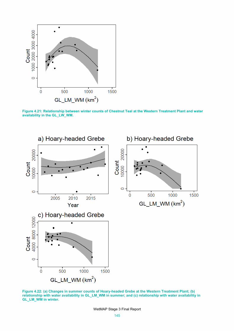
WetMAP Stage 3 Final Report
145
Figure 4.21: Relationship between winter counts of Chestnut Teal at the Western Treatment Plant and water availability in the GL_LW_WM.
Figure 4.22: (a) Changes in summer counts of Hoary-headed Grebe at the Western Treatment Plant; (b) relationship with water availability in GL_LM_WM in summer; and (c) relationship with water availability in GL_LM_WM in winter.

WetMAP Stage 3 Final Report
146
Figure 4.23: (a) Changes in numbers of Australian Shelduck at the Western Treatment Plant through time; (b) relationship with water availability in GL_ML_WM area in summer; (c) relationship with water availability in the Lower Murray in winter.
Figure 4.24: Annual summer counts of Eurasian Coot at the Western Treatment Plant through time.

WetMAP Stage 3 Final Report
147
Figure 4.25: (a) Summer counts of Blue-billed Duck at the Western Treatment Plant through time; (b) relationship with water availability in GL_LM_WM; (c) relationship with water availability in LOWER_MURRAY.
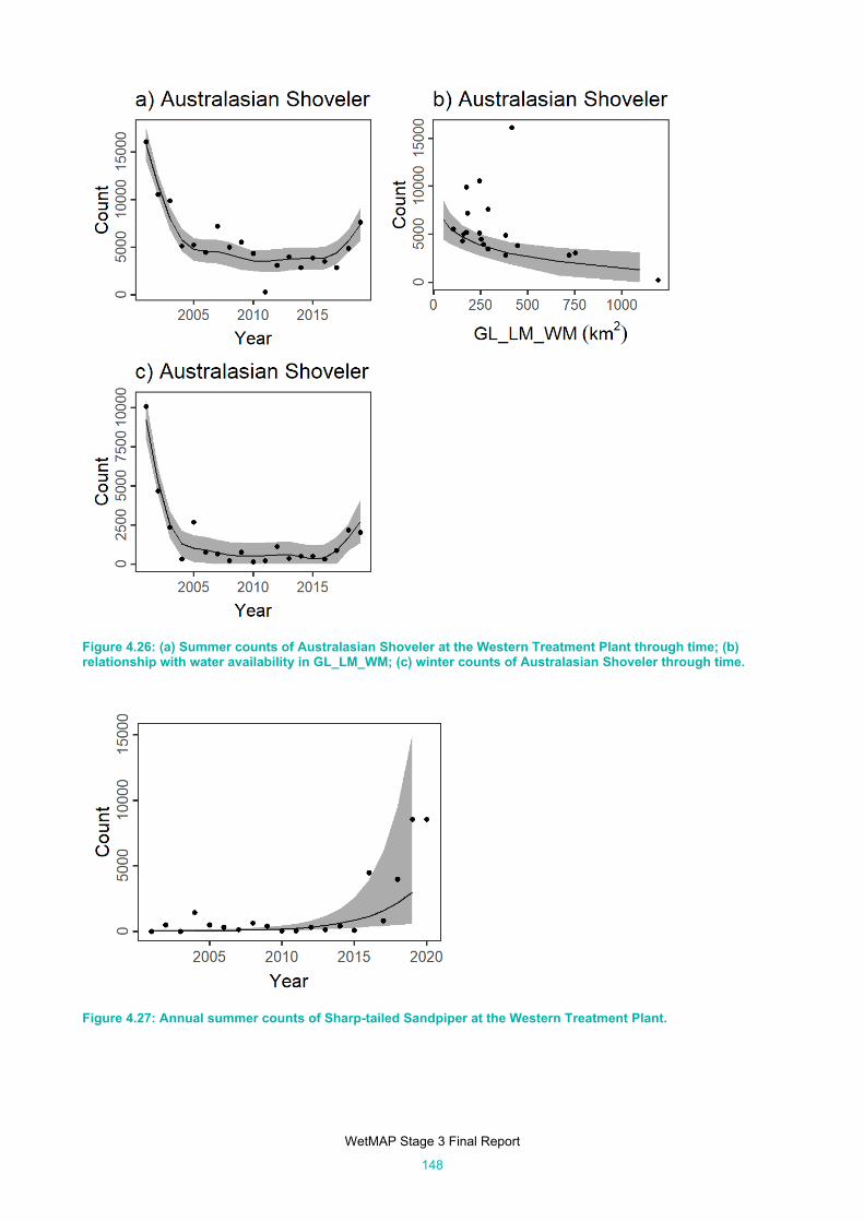
WetMAP Stage 3 Final Report
148
Figure 4.26: (a) Summer counts of Australasian Shoveler at the Western Treatment Plant through time; (b) relationship with water availability in GL_LM_WM; (c) winter counts of Australasian Shoveler through time.
Figure 4.27: Annual summer counts of Sharp-tailed Sandpiper at the Western Treatment Plant.

WetMAP Stage 3 Final Report
149
Figure 4.28: (a) Summer counts of Whiskered Tern at the Western Treatment Plant through time; (b) relationship with water availability in GL_LM_WM.
Discussion
Responses of waterbird abundance and species richness to environmental water events (KEQ 1)
There were more waterbirds and higher waterbird species richness in wetlands that held water. This environmental water response was consistent across all seasons, indicating that flow releases had positive benefits regardless of timing. However, waterbird numbers and species richness were highest in spring and (especially) summer, indicating that water releases will have more benefits for waterbirds if they are strategically timed to coincide with the natural peaks in numbers in Victoria.
The strength of waterbird response to environmental water appeared to be stronger at some sites (e.g. Gaynor Swamp, Heywood’s Lake, Lake Murphy, McDonalds Swamp, Reedy Swamp) than at others (e.g. Black Swamp, Vinifera Floodplain; Figure 4.12). Sites with stronger responses tended to be those where more water was present on the day of sampling. For example, except for McDonalds Swamp, the average wet proportion of samples taken during the wet phases for the other sites was greater than 50% (i.e. more than 50% of the wetland was wet). In comparison, the wet proportion tended to be lower at sites with less pronounced responses, for example Black Swamp (mean wet proportion of 25% during wet samples), Hird Swamp East (mean wet proportion 9%), Vinifera Floodplain (29%) and Wirra-Lo (37%). A longer time series would allow the potential drivers of this variability to be explored.
It is important to note that we used 5% as our cut-off to distinguish wet and dry hydrological phases. These cut-offs were selected to make sure that the distinctions between wet and dry phases were clearly distinguishable, that is, a cut-off of 1% might have resulted in ambiguities about whether samples were in dry or wet phases This means that our counts are likely to potentially overestimate numbers on completely dry wetlands, especially as there was often a small concentration of waterbirds in the last remaining puddles of wetlands that were drying out. As a point of comparison, we present some further summaries (Table 4.7) illustrating that few birds were counted (only 92 in total) at sites with a wet proportion of zero (i.e. completely dry) compared with sites with a wet proportion in the range 1–5%.
In the comparisons between dry and wet wetlands, we have evaluated short-term responses to watering. Further study is needed to better understand responses in the longer term. This is particularly important considering environmental watering is likely to cause changes in vegetation that could alter the capacity to support waterbirds in the long term. For example, most shorebird species have a strong preference for open habitats in which vegetation is less than half their height (Helmers 1992; Rogers et al. 2015) but prolonged shallow flooding in freshwater wetlands stimulates the growth of tall dense vegetation, which shorebirds avoid (Isola et al. 2000; Rogers et al. 2015). It is important to consider the longer-term causal pathways from watering to ultimate net population outcomes for birds, for example changes in habitat structure, food availability and

WetMAP Stage 3 Final Report
150
ultimately breeding success. Our conceptual models highlight some of these pathways, and we have begun to explore them with the data collected to date. The analyses undertaken for SQs 1–3 provide support for some of the proposed hypotheses, or at least suggest that the questions can be answered with longer data series. As an example, we predicted that waterbird numbers and diversity would drop off when wetlands were flooded permanently (Figure 4.4), because we anticipated that such regimes would lead to denser fringing vegetation (avoided by many waterbirds), a reduction in the amount of edible aquatic vegetation, and a reduction in accessible infaunal prey in shallow waters. The general additive mixed model did indeed indicate that waterbird abundance dropped off in watered wetlands that had been deeply filled for extended periods (Figure 4.17b). This generalisation is unlikely to apply to wastewater treatment plants, despite their permanent water regimes; they held high densities of waterbirds, presumably in part because they are nutrient enriched and in part because dense vegetation cannot get established along their steep banks due to active vegetation control.
Table 4.7: Mean numbers of waterbirds and guilds per survey in wetlands that were completely dry, near-dry and wet.
Guild Completely dry Water cover between 1
and 5% Water cover >5%
Overall numbers 5.6 54.2 1510.2
Large Waders 2.4 2.7 48.1
Shallow Waterfowl 0.75 35.8 994.2
Deep Waterfowl 0 0 201.3
Skulkers 1.9 8.0 14.9
Shorebirds 0.5 5.6 108.5
Swimming Piscivores 0.1 2.2 80.1
Terns 0 0 62.3
Response of waterbird breeding to environmental water at wetlands (KEQ 2)
We found very few cases of breeding given the scale of the survey program: during the entire survey period we recorded 662,496 waterbirds (71 species) in watered wetlands, but only 102 of our observations (12 species) involved birds confirmed to be breeding. While we are unlikely to have overlooked nesting by conspicuous colonially nesting species, it is possible that some other breeding events (especially by dispersed, cryptic species) at the wetlands were overlooked, given that our search methods for nesting birds were not intensive. In addition, it is likely that some terrestrial bird species nested in some of the habitats provided by wetlands, especially in hollows in stags. However, reasonable correction of our confirmed observations of breeding to account for limitation in sampling is not likely to yield breeding at a scale required to support the populations observed, that is, it is extremely unlikely that there was sufficient recruitment at our study sites to balance annual mortality of adult waterbirds. Global reviews indicate that annual apparent survival ranges from 40 to 80% in wildfowl (Krementz et al. 1997) and from 48 to 98% in shorebirds (Mendez et al. 2018). Moreover, a large proportion of the breeding records that were obtained came from a small number of wetlands. It is pertinent to ask why so few birds nested in watered wetlands, and why they were apparently quite localised.
Most breeding records came from wetlands that had been wet for over a year (Lake Murphy, Johnson Swamp, Reedy Swamp, Round Lake, Shepparton and Swan Hill wastewater treatment plants), and there were few or no breeding records from sites that were wet for less than a year (e.g. Gaynor Swamp, Black Swamp, Moodie

WetMAP Stage 3 Final Report
151
Swamp, Vinifera Floodplain, and Wirra-Lo Lignum Swamp). This should not be considered evidence that waterbirds cannot breed in wetlands immediately after they have been flooded; there is abundant evidence that breeding waterbirds can exploit recently flooded wetlands in other regions of Australia (e.g. Maher 1991; Briggs 1992; Briggs et al. 1997; Bino et al. 2015; Pedler et al. 2017). However, the watered wetlands of Victoria are not necessarily directly comparable with the naturally watered floodplain and salt-lake sites used in those studies. Our study sites are rather small wetlands; the environmental water allocation to them was often lower than that which would be observed in a natural flooding event; and they were isolated events (unlike natural flooding events, which would likely be associated with flooding of many nearby wetlands).
Rogers (2019) proposed several hypotheses (not mutually exclusive) that may explain why so few waterbirds bred in watered WetMAP wetlands during the study period.
1. Environmental watering did not produce suitable vegetation structure and food availability for waterbird breeding. If this were the case, alteration of water management regimes within wetlands could potentially be used to improve the suitability of local habitats for waterbird breeding.
2. WetMAP studies were not undertaken in wetlands suitable for waterbird nesting. Selection of WetMAP sites only considered sites that could be monitored repeatably through waterbird counts; such sites tended to be small and isolated, with limited tall vegetation. Therefore, breeding events may have been missed at more complex wetlands with denser vegetation that were not part of the set of wetlands monitored.
3. Wetlands were not watered for long enough for successful breeding to occur. In many watered wetlands, there are limitations to flow rate and duration that prevent wetlands being completely filled, thus reducing the period they hold water before drying out. Rogers (2010) reviewed the duration of flooding required by waterbirds for successful breeding and these estimates could be used as a starting point in assessing whether flood duration at WetMAP sites is long enough for waterbirds to breed successfully.
4. Waterbirds did not initiate breeding in watered wetlands because they made an early-season assessment that the wetland would dry out before they could raise chicks. Whether waterbirds are capable of such strategic planning is unknown, but this hypothesis could potentially explain why waterbirds did not breed at apparently suitable sites such as Gaynor Swamp. Gaynor Swamp was flooded for long enough for waterbirds to nest and raise young, but the water was provided in three flows (511 ML in autumn, 512 ML in spring and 100 ML in midsummer). At the start of the breeding season, in early spring, waterbirds would not have been aware that additional flows would be allocated to the wetland. If this mechanism does affect the initiation of waterbird breeding, we would predict a higher incidence of waterbird breeding in wetlands where waterbirds have cues that there will be a prolonged period of flooding. Such cues could include deep and extensive initial flooding of wetlands. Prior experience of particular sites might also influence waterbird perceptions of the likely duration of fill.
5. Waterbirds assess water availability on a regional scale (not only at the wetland where they wish to nest) before making the decision to breed; they defer breeding if they perceive that there is insufficient water in the region for fledged young to survive until breeding age. Again, it is not known whether waterbirds are capable of such strategic planning.
Rogers et al. (2019) suggested several approaches to testing these hypotheses. Helpful insights could be obtained from additional local response monitoring, deeper analysis of the habitat data already collected, and comparison of historical breeding records with satellite-derived data on extent and duration of flooding. Remote-tracking studies were identified as a tool particularly suitable to address Hypotheses 1 and 2 (relating to identification of the habitat attributes required by breeding waterbirds) and Hypothesis 5 (whether waterbirds assess water availability on a regional scale before making the decision to breed).
These hypotheses are of particular interest because of their potential implications for management of watered wetlands. For example, with a better understanding of breeding habitat requirements, it may be possible to alter the timing, duration or frequency of watering events to increase the likelihood that managed wetlands will be used by breeding waterbirds. On the other hand, if it proves that waterbirds base their decision on whether to breed on water availability on a broad regional scale, it is unlikely that environmental watering of small isolated wetlands during dry years would result in breeding outcomes. If this were the case, it may be necessary to review Environmental Watering Plans, accord waterbird breeding lower priority than more

WetMAP Stage 3 Final Report
152
achievable ecological objectives or investigate the possibility that local clusters of wetlands need to be watered concurrently to stimulate breeding by waterbirds.
Changes in waterbird habitat following watering events (KEQ 3) We found clear evidence that environmental water increased suitable habitat for waterbirds. There were significant relationships between the extent of different habitat types and stage of environmental watering. Not surprisingly, the extent of Deep Open Water, Shallow Open Water, Shallow Water with Emergent Plants, Aquatic Vegetation and Bare Wet Substrate were higher in wetlands when they held water. These differences were significant, despite the categorisation of a few near-dry wetlands (holding <5% water) as dry; an even clearer difference would have been apparent had we excluded wetlands with 1–5% water cover from the analysis. In contrast, the extent of River Red Gum and Tall Marsh within wetlands was similar in wetlands when they were wet and when they were dry.
All waterbird species showed structural habitat preferences, these preferences differing between species. Deep Open Water was preferred by Deep Waterfowl and Swimming Piscivores; Shallow Open Water and Shallow Water with Emergent Plants were preferred by most species of Shallow Waterfowl and Large Waders; Shorebirds preferred Shallow Open Water or Bare Wet Substrate; Skulkers showed a preference for Shallow Water with (dense) Emergent Plants. The extent of these habitats was higher when wetlands held environmental water.
Waterbird activity (both foraging and not foraging) was recorded at the same time as habitat use. Our data demonstrated that both foraging and roosting habitat increased in extent with environmental water; they also demonstrated that waterbirds had tighter habitat preferences when foraging. Habitat use by breeding birds could not be evaluated fully because of the small number of breeding records.
While convenient for analysis, the ‘Wet vs Dry’ analysis used to address KEQ 1 was rather simplistic. Further analysis of the data we have collected could provide a quantitative assessment of how structural habitat in wetlands changes according to depth, duration and frequency of environmental watering. At local scales, this kind of information would be helpful for management, enabling predictions to be made about how waterbird habitats will change during a watering event. The details are likely to differ between wetlands, according to the type of vegetation that they hold. In addition, a quantitative understanding of how waterbird habitat changes through the watering cycle would enable testable predictions for two key questions; (1) what waterbird species are likely to be attracted to specific wetlands following environmental watering; (2) in what numbers are they are expected to occur.
While our results have shown that environmental water events are likely to change the availability of habitats used by different waterbirds, it is important to also consider the potential impacts of other factors that will influence habitat availability. These include previous watering history, and management of wetlands during their dry periods, when vegetation could be impacted by factors such as grazing, fire or weed invasion. It will therefore be important to consider the potential need for integrated management of wetlands, considering not only water requirements, but also possible threats to wetlands.
Responses of woodland birds adjacent to wetlands to environmental water events (KEQ 4)
Vegetation in the woodlands fringing wetlands includes plants that require occasional flooding or may draw on groundwater provided by environmental watering (e.g. River Red Gum, Black Box). Moreover, many insects have aquatic larval phases likely to benefit from environmental watering, and their terrestrial adult phases can be abundant in the vegetation surrounding wetlands. We therefore though it was possible that the benefits of environmental watering to birds could extend beyond the limits of surface water to the woodlands surrounding water bodies. However, delivery of environmental water (Figure 4.16) had no detectable short-term effect on the number of birds, or number of bird species, in the woodlands fringing watered wetlands. We doubt that further collection of the same kind of data would provide new insights.
Although our surveys showed there is a high diversity of woodland birds in the woodlands fringing some WetMAP sites, only 6 of the 116 species (~5%) recorded are listed as threatened or near-threatened, and all of these also make use of other habitats. In contrast, waterbirds show clear positive responses to environmental watering, and 24 of the 71 waterbird species (~34%) recorded at WetMAP sites are listed as threatened or near-threatened, and these species are restricted to wetlands. It is likely that waterbirds will be

WetMAP Stage 3 Final Report
153
given higher priority than terrestrial birds when making annual decisions on water allocations to watered wetlands.
We therefore suggest that WetMAP discontinues regular surveying of terrestrial birds in the woodlands fringing watered wetlands. The time that could be saved from this work could be better used on other questions, for example surveying waterbirds at a larger number of sites.
The woodland bird data collected for WetMAP will be lodged and made publicly available in the Victorian Biodiversity Atlas (https://www.environment.vic.gov.au/biodiversity/victorian-biodiversity-atlas) and the Birdata databases of BirdLife Australia (https://birdata.birdlife.org.au/explore#map=-22.5083100_136.0786120_4). It should therefore be available to researchers in future years who may be able to address whether environmental watering has long-term effects on woodland birds that could not be detected by our 3-year study. We also note that monitoring of indicators of woodland health (see vegetation theme chapter) will provide some information on the habitat available to woodland bird species. Woodland species will be dependent on woodlands, and a transition from woodland to non-woodland vegetation (mass tree death) or a transition from non-woodland to woodland (mass tree recruitment) would likely also transition the fringing bird community.
Exploration of relationships with hydrological regimes (SQ 1–3) While there was strong evidence that provision of environmental water was beneficial to waterbirds, management decisions should ideally be based on a more detailed understanding of the quantitative responses of waterbirds to volume, timing and interval of watering events. The models presented in this report are encouraging in that they demonstrate significant relationships between waterbird abundance and a range of hydrological variables.
Broadly, the number of waterbirds in a wetland was related to its area and the duration of the antecedent period for which the wetland held water. The antecedent period for which watering has the strongest influence appears to differ between species. For example, numbers of Hoary-headed Grebe were most strongly related to the proportion of wetland that was flooded at the time of survey; numbers of Black-winged Stilt were most strongly related to the proportion of wetland that had been flooded over the past 30 days, and numbers of Black Swan were most strongly related to the proportion of wetland that had been flooded over the past 90 days. It is possible that these interspecific differences were related to diet and foraging behaviour, and the dependence of feeding habitat and food availability on the different hydrological characteristics. Hoary-headed Grebes can forage in deep water and feed largely on swimming aquatic invertebrates, which are likely to colonise wetlands quickly; Black-winged Stilts forage in part on benthic infauna, which is likely to take longer to become established, and further require water 5–15 cm deep, so may need water levels to recede a little before they can forage; Black Swans feed on aquatic vegetation, which takes some time to grow after flooding.
Some variables were not as strongly supported in the models as we anticipated. Season was not identified as a significant factor, but there was evidence that more waterbirds were present in spring and summer than at other times (e.g. Figure 4.2, Figure 4.11). While there was support for area of wetland being important to all species, there were some species in which wetland area was not in the most strongly supported model. Further analyses and/or longer datasets may be needed to clarify the roles of these variables. For example, our samples in some seasons (notably late autumn and early spring) were smaller than those in late spring and summer, in part from logistic constraints and in part because watering schedules in several wetlands did not involve winter fills. It is therefore possible that our smaller samples at these times led to broad confidence intervals that obscured seasonal trends.
The weakly significant relationship between wetland area and number of waterbirds merits further investigation, and it is possible that a more nuanced categorisation of wetlands is required; perhaps not all watered wetlands can be considered the same ‘type’. Wastewater treatment plants supported higher densities of waterbirds than the watered wetlands we studied, and perhaps within the environmental wetlands some sites should be classified as more productive than others. Further examination of the zooplankton and water quality data obtained for WetMAP may be illuminating. Bathymetry of wetlands also needs careful examination. Water depth is likely to be a key variable for many waterbird species; for example, Rogers and Hulzebosch (2014) found that different shorebirds chose water of different depths, each preferring a particular, narrow band of water depths. The unique bathymetry of each wetland may mean that water cover is a poor proxy for water-depth heterogeneity; these intricacies are not reflected perfectly by water cover, the measure of habitat availability used in these analyses. Water-depth data were collected by the WetMAP project, and data from depth loggers is currently being consolidated. Coupled with information on the bathymetry of each wetland,

WetMAP Stage 3 Final Report
154
these data could provide a much more refined index of effective habitat area for particular waterbird species. The potential relationships between water depth, wetland bathymetry and density of vegetation may also need to be considered to reach the point where it is possible to make good predictions of the number of waterbirds likely to move into specific wetlands in response to environmental watering events.
Are waterbird abundance and species richness affected by continental rainfall patterns and water availability in the Australian landscape? (SQ 4)
Our analysis of long-term waterbird count data from a Victorian site (the WTP) successfully demonstrated that local waterbird abundance and species diversity are affected by continental rainfall patterns and water availability in the Australian landscape. Unlike previous studies, we used a direct measure of water availability in key wetland systems in several of eastern Australia’s drainage basins (as estimated by GA on the basis of satellite imagery), rather than a continent-wide index of water availability. It is probably for this reason that our study is one of the first to detect species-specific relationships dependent on water availability in particular regions. In several species (e.g. Pink-eared Duck, Freckled Duck, Hoary-headed Grebe and Australian Shelduck), numbers at the WTP were more strongly related to water availability in the Goulburn–Loddon, Wimmera and Mallee catchments than to water availability in any other catchment areas, suggesting that this region is of greater importance to WTP waterbirds than (for example) the Namoi–Gwydir.
Ornithologists have long assumed that fluctuations in waterbird numbers in southern Victoria reflect responses to inland rainfall (Chambers and Loyn 2006; Loyn et al. 2014; Hansen et al. 2015); there have been analyses demonstrating negative relationships between waterbird numbers in Victorian coastal refugia (including the Western Treatment Plant) with rainfall and streamflow in the Murray–Darling Basin (Clarke et al. 2015), and with soil moisture and streamflow in inland Australia (Clemens 2017). However, the effects of the distribution of inland surface water availability on numbers of waterbirds in Victorian wetlands are less well understood. There are reasons to suspect it may be of importance. While the natal origins of waterbirds in non-breeding refugia in Victoria’s wetlands are poorly known, it is known that most Australian waterbirds differ to some extent in their distribution (Barrett et al. 2003). It is also known that trends over time differ between many waterbird species. The WTP data that we analysed, for example, demonstrated increases in Australian Shelduck, decreases in Australasian Shoveler and complex non-linear changes over time in species such as Eurasian Coot. Potentially, such interspecific differences could be driven by differences in preferred breeding areas, with breeding success (and hence population growth or decline) related to water availability in key breeding regions.
A recent analysis by Bino et al. (2020) emphasised strong synchronicity of counts (from aerial surveys) of ducks in the Murray–Darling Basin and Lake Eyre Basin, and showed there was strong correlation of rainfall between catchments. However, this does not necessarily mean that water availability is strongly correlated between catchments. Bino et al. (2020) pointed out that streamflow between catchments was quite weakly correlated, in large part because river regulation in the Murray–Darling Basin has altered the connections between rainfall and stream flow. Stream flow is an indirect measure of water availability from the perspective of waterbirds; there are lags between rainfall and stream flow (Clarke et al. 2015), and most Australian waterbirds nest in wetlands rather than in waterways. The amount of water in the wetlands used by waterbirds is likely to be geographically influenced by landforms and evaporation in addition to rainfall and flow.
Our analyses were undertaken as a ‘test of concept’ and could be extended and refined. Comparison with models that use rainfall or streamflow as the index of water availability would be useful in assessing whether use of surface water offers more precision when trying to identify correlates with Victorian numbers. It would be of interest to carry out similar analyses on a wider range of species, and to compare count data with water cover data from more sites in inland (and northern) Australia. A finer temporal breakdown of data (e.g. by month rather than by year) may provide additional insights on the likely origins of the waterbirds that occur in watered wetlands.
Waterbirds are highly mobile, and the number present within a wetland is influenced both by attributes of the wetland and by factors that are beyond the control of wetland managers (e.g. availability of inundated wetlands in other parts of the landscape). At least for some species of waterbird, this may lead to circumstances in which investment in environmental watering fails to generate waterbird outcomes at the anticipated magnitude because of high availability of inundated wetlands in other parts of eastern Australia. Consequently, when planning where to allocate environmental water in which years, it would be desirable to be able to predict better how waterbirds will respond given actual or forecast water availability in wetlands across eastern Australia.
In the long term, we envisage development of quantitative models to predict the expected outcome (numbers of waterbirds ± confidence intervals) of environmental water delivery to wetlands, based on the types of relationships tested here. Such models could inform decisions on when and where to allocate environmental

WetMAP Stage 3 Final Report
155
water each year and provide a quantitative target against which to assess whether environmental watering events achieved the desired effect on waterbird numbers, given the year’s conditions Australia-wide. Models of this kind would be informed by:
WetMAP Stage 3 Final Report
156
previous counts at the wetland and in the broader region
the size and habitat attributes of the wetland, and waterbird responsiveness to watering
time of year
availability of alternate wetland habitat in the local region
availability of alternate wetland habitat in the broader Australian landscape.
The WetMAP Bird theme plan 2019–2020 (Rogers 2019) proposed a broad approach to collecting the necessary information needed to develop these models. It includes recommendations for remote-tracking work to fill gaps in our knowledge of where waterbirds breed, the habitats they use, and the manner in which they respond to water availability at alternative sites at both local and regional scales.
Conclusions and future directions
Applied considerations for future research WetMAP Stage 3 has demonstrated strong short-term benefits of environmental water to waterbirds. It has also demonstrated factors that affect the strength of this response: they include season, structural habitats available within the wetland, hydrological regime within wetlands, and surface water availability in other parts of Australia. Although waterbirds certainly moved into wetlands when they received environmental water, rather few waterbirds nested in the wetlands that we studied.
A challenge ahead is working out how to refine and translate our evolving understanding into tangible guidelines for wetland managers. Even with existing Environmental Watering Plans, managers need to make annual decisions about how to manage environmental water allocations to selected wetlands. Questions relevant to these local decisions include:
1. When should environmental water be delivered to wetlands?
2. How much water is needed?
3. How often should wetlands be surveyed to assess the effects of watering?
4. When should these surveys be carried out?
5. How should water be managed to increase the likelihood of waterbird breeding?
6. Cumulative effects of previous watering: i.e. will another season of watering improve or diminish structural vegetation attributes of the site?
Improved understanding of the answers to these questions would also allow wetland managers to better assess the success, or otherwise, of environmental watering. Waterbird counts are likely to remain the preferred measure of the success of environmental watering, but they are not always easy to interpret. For example, is a count of 1000 Grey Teal at a particular wetland an indication that environmental watering has been successful? The answer to this question is dependent on context: e.g. the size of the wetland, the number of birds it typically supports, and the extent to which counts in a particular year might have been influenced by the factors identified above (e.g. season, structural habitats, hydrological regime, population trends and water availability elsewhere in Australia). Depending on the answers to these questions, a count of 1000 Grey Teal might be considered highly successful, or an indication that management of the wetland could be improved to better support this species. Models that draw together the information outlined above to predict how many waterbirds would be expected in a wetland in a given year would be a powerful management tool.
Environmental Watering Plans consider the management of particular wetlands, rather than the co-ordination of watering between wetlands. For waterbirds, these considerations may be important. A number of studies (including this report) indicate that waterbird numbers and diversity in Victoria are highest in years when drought has reduced the availability of inland wetlands: in drought years the additional habitat provided by environmental water is likely to be of higher importance to waterbirds.
The strong selection by different waterbird species for different structural wetland habitats shown in this study raises another strategic issue. Should we manage wetlands to maximise waterbird numbers and density? Or would it be of broader conservation value to manage these wetlands so that they provide waterbird habitat of a kind that is poorly represented in other wetlands of Victoria? For example, ducks are the most numerous waterbirds in most e-watered wetlands; they have a strong preference for open water which is also extensively available in other wetlands (such as water treatment plants). Bitterns are far less numerous and have a strong preference for wetlands that hold Tall Marsh and Shallow Water with emergent plants. It is likely that there is

WetMAP Stage 3 Final Report
157
little suitable habitat for them outside watered wetlands, but there is no solid data on this. A better understanding of the availability of different wetland types elsewhere in Victoria could help managers to decide whether managing wetlands for Bitterns is of higher conservation value than managing them for much larger numbers of ducks.
Next steps The next step for the WetMAP bird theme will be a re-evaluation of the KEQs and SQs to guide the next stage of the project. We have outlined several potential avenues for future work above. These will be further developed and evaluated over the coming months. Local response monitoring will remain a core activity of the bird theme of WetMAP, providing monitoring information of immediate use to the CMAs, and building the dataset on which models predicting waterbird responses can be based. Discussion will also focus on additional potential research directions that may complement this work. They include satellite tracking of selected species to refine understanding of movements, habitat and breeding requirements, and potentially broader-scale wetland surveying to assess availability of alternate habitat to waterbirds within Victoria.
References Alcorn, M., Alcorn, R. and Fleming, M. (1994). Wader movements in Australia: final report of the regular counts
project 1981–1990. Australasian Wader Studies Group. RAOU Report No. 94.
Barrett, G., Silcocks, A., Barry, S., Cunningham, R. and Pulter, R. (2003). The New Atlas of Australian Birds. Royal Australasian Ornithologists Union, Hawthorn East, Victoria.
Bino, G., Kingsford, R.T. and Porter, J. (2015). Prioritizing wetlands for waterbirds in a boom and bust system: waterbird refugia and breeding in the Murray–Darling Basin. PLoS ONE 10, e0132682. doi:10.1371/journal.pone.0132682
Bino, G., Brandis, K., Kingsford, R.T. and Porter, J. (2020). Waterbird synchrony across Australia’s highly variable dryland rivers – risks and opportunities for conservation. Biological Conservation 243, 108497.
Brandis, K.J., Bine, G., Spencer, J.A., Ramp, D. and Kingsford, R.T. (2018). Decline in colonial waterbird breeding highlights loss of Ramsar wetland function. Biological Conservation 225: 22–30.
Briggs, S.V. (1992). Movement patterns and breeding characteristics of arid zone ducks. Corella 16: 5–22.
Briggs, S.F., Thornton, S.A. and Lawler, W.G. (1997). Relationships between hydrological control of River Red Gum wetlands and waterbird breeding. Emu 97: 31–42.
Chambers, L.E. and Loyn, R.H. (2006). The influence of climate variability on numbers of three waterbird species in Western Port, Victoria, 1973–2002. International Journal of Biometeorology 50, 92–304.
Clarke, R.H., Herrod, A., Loyn, R.H., Carter, M.J., Silcocks, A., Menkhorst, P. and Johnstone, C. (2015). Waterbird fluctuations at coastal wetland refugia in response to Murray–Darling Basin streamflow and rainfall. Prepared for Melbourne Water by Monash University, Victoria.
Clemens, R.S., Rogers, D.I., Hansen, B.D., Gosbell, K.G., Minton, C.D.T., Straw, P.,Bamford, M., Woehler, E.J., Milton, D., Weston, M.A., Venables, W., Weller, D., Hassell, C., Rutherford, W., Onton, K, Herrod, A., Studds, C.E., Choi, C-Y., Dhanjal-Adams, K., Murray, N. J., Skilleter, G. and Fuller, R.A. 2016. Continental-scale decreases in shorebird populations in Australia. Emu 116, 119-135.
Clemens, R.S. (2017). Ecology and conservation of Australia’s shorebirds. PhD Thesis, School of Biological Sciences, University of Queensland. doi:10.14264/uql.2017.610
Cresswell, W. (2008). Non-lethal effects of predation risk in birds. Ibis 150, 3–17.
Ekanayake, K.B., Whisson, D.A., Tan, L.X.L. and Weston, M.A. (2015). Intense predation of non-colonial, ground-nesting bird eggs by corvid and mammalian predators. Wildlife Research 42 (6), 518–528.
Frith, H.J. (1982). Waterfowl in Australia. Angus and Robertson, Sydney, New South Wales.
Halse, S.A., Williams, M.R., Jaensch, R.P. and Lane, J.A.K. (1993). Wetland characteristics and waterbird use of wetlands in south-western Australia. Wildlife Research 20 (1), 103–125.
Hamilton, A.J. and Taylor, I.R. (2004). Seasonal patterns in abundance of waterfowl (Anatidae) at a waste stabilization pond in Victoria. Corella 28, 61–67.

WetMAP Stage 3 Final Report
158
Hansen, B.D., Menkhorst, P., Maloney, P. and Loyn, R.H. (2015). Long-term declines in multiple waterbird species in a tidal embayment, south-east Australia. Austral Ecology 40, 515–527.
Helmers, D.L. (1992). Shorebird Management Manual. Western Hemisphere Shorebird Reserve Network, Manomet, USA.
Isola, C.R., Colwell, M.A., Taft, O.W. and Safran, R.J. (2000). Interspecific differences in habitat use of shorebirds and waterfowl foraging in managed wetlands of California’s San Joaquin Valley. Waterbirds 23, 196–203.
Kingsford, R. T. , and Thomas, R. F. (1995). The Macquarie Marshes and its waterbirds in arid Australia: a 50-year history of decline. Environmental Management 19, 867–878.
Kingsford, R.T. and Thomas, R.F. (2004). Destruction of wetlands and waterbird populations on the Murrumbidgee River in arid Australia. Environmental Management 34, 383–396.
Kingsford, R.T., Bino, G. and Porter, J.L. 2017. Continental impacts of water development on waterbirds, contrasting two Australian river basins: Global implications for sustainable water use. Global Change Biology 23, 4958-4969.
Kingsford, R.T, Roshier, D.A. and Porter, J.L. (2010). Australian waterbirds – time and space travellers in dynamic desert landscapes. Marine and Freshwater Research 2010 (61), 875–884.
Krementz, D.G., Barker, D.J. and Nichols, J.D. (1997). Sources of variation in waterfowl survival rates. Auk 114, 93–102.
Lank, D.B. and Ydenberg, R.C. (2003). Death and danger at migratory stopovers: problems with “predation risk”. Journal of Avian Biology 34, 225–228.
Loyn, R.H., Dann, P. and Bingham, P. (1994). Ten years of waterbird counts in Western Port, Victoria, 1973–83. 1. Waterfowl and large wading birds. Australian Bird Watcher 15, 333–350.
Loyn, R.H., Rogers, D.I., Swindley, R.J., Stamation, K., Macak, P. and Menkhorst, P. (2014). Waterbird monitoring at the Western Treatment Plant, 2000–12: the effects of climate and sewage treatment processes on waterbird populations. Arthur Rylah Institute for Environmental Research Technical Report Series No. 256. Department of Environment and Primary Industries, Heidelberg, Victoria.
Maher, M. (1991). Waterbirds back o’ Bourke: an inland perspective on the conservation of Australian waterbirds. PhD Thesis, University of New England, New South Wales.
Marchant, S. and Higgins P.J. (eds) (1990). Handbook of Australian, New Zealand and Antarctic Birds. Volume 1: Ratites to Ducks. Oxford University Press, Melbourne, Victoria.
Marchant, S. and Higgins P.J. (eds) (1993). Handbook of Australian, New Zealand and Antarctic Birds. Volume 2: Raptors to Lapwings. Oxford University Press, Melbourne, Victoria.
Mauser, D.M., Jarvis, R.L. and Gilmer, D.S. (1994). Survival of radio-marked Mallard ducklings in northeastern California. Journal of Wildlife Management 58, 82–87.
Mendez, V., Alves, J.A., Gill, J.A. and Gunnarsson, T.G. (2018). Patterns and processes in shorebird survival rates: a global review. Ibis 160, 723–741.
Nebel, S. , Porter, J. L. , and Kingsford, R. T. (2008). Long-term trends of shorebird populations in eastern Australia and impacts of freshwater extraction. Biological Conservation 141, 971–980.
Pedler, R., Ribot, R.F.H. and Bennett, A.D.T. (2017). Long-distance flights and high-risk breeding by nomadic waterbirds on desert salt lakes. Conservation Biology 32, 216–228.
Reid, J. (2009). Australian Pelican: flexible responses to uncertainty. In: Robin, L., Heinsohn, R. and Joseph, L. (Eds) Boom and Bust. Bird Stories for a Dry Country, pp. 95–120. CSIRO Publishing, Canberra, ACT.
Reynolds, M.H. and Work, T.M. (2005). Mortality in the endangered Laysan Teal Anas laysanensis: conservation implications. Wildfowl 55, 31–48.
Ricklefs, R.E. (1969). An analysis of nesting mortality in birds. Smithsonian Contributions to Zoology 9, 1–48.

WetMAP Stage 3 Final Report
159
Rogers, D. (2019). Project plan: 2019–20 WetMAP bird theme 2019–20 monitoring bird response to environmental water delivery in Victoria. Prepared for Water and Catchments, Department of Environment, Land, Water and Planning, Heidelberg, Victoria.
Rogers, D., Purdey, D., Stamation, K., Quin, D. and Upton, R. (2019). WetMAP Bird Theme Annual Report 2019. Arthur Rylah Institute for Environmental Research, Department of Environment, Land, Water and Planning, Heidelberg,
Rogers, D.I., Hance, I., Paton, S., Tzaros, C., Griffioen, P., Herring, M., Jaensch, R., Oring, L., Silcocks, A. and Weston., M. (2005). The breeding bottleneck: breeding habitat and population decline in the Australian Painted Snipe. In Straw, P. (Ed.) Status and conservation of shorebirds in the East Asian – Australasian Flyway. Proceedings of the Australasian Shorebirds conference, Canberra, 13–15 December 2003, pp. 15–23. Wetlands International Global Series 18, International Wader Studies 17, Sydney.
Rogers, D. and Hulzebosch, M. (2014). Use of non-tidal ponds by shorebirds at the Western Treatment Plant. Arthur Rylah Institute for Environmental Research. Unpublished client report for Melbourne Water. Department of Environment and Primary Industries, Heidelberg, Victoria.
Rogers, D.I., Stamation, K.S. and Menkhorst, P. (2015). Literature review: management of non-tidal ponds for shorebirds. Arthur Rylah Institute for Environmental Research Technical Report No 264. Department of Environment, Land, Water and Planning, Heidelberg, Victoria.
Rogers, K. (2010). Waterbirds. In: Rogers, K. and Ralph, T. (Eds) Floodplain Wetland Biota in the Murray–Darling Basin. Water and Habitat Requirements. CSIRO Publishing, Clayton, Victoria.
Roshier, D. (2009). Grey Teal: survivors in a changing world. In: Robin, L., Heinsohn, R. and Joseph, L. (Eds) Boom and Bust. Bird Stories for a Dry Country, pp. 75–94. CSIRO Publishing, Canberra, ACT.
Sargeant, A.B. and Raveling, D.G. (1992). Mortality during the breeding season. In: Batt, B.D.J., Afton, A.D., Anderson, M.G., Ankney, C.D., Johnson, D.H., Kadlec, J.A. and Krapu, G.L. (Eds) Ecology and Management of Breeding Waterfowl, pp. 396–422. University of Minnesota Press, Minneapolis, USA.
Sedinger, J.S. (1992). Ecology of prefledging waterfowl. In: Batt, B.D.J., Afton, A.D., Anderson, M.G., Ankney, C.D., Johnson, D.H., Kadlec, J.A. and Krapu, G.L. (Eds) Ecology and Management of Breeding Waterfowl, pp. 109–127. University of Minnesota Press, Minneapolis, USA.
Taylor, I.R. (2003). Australia’s temporary wetlands: what determines their suitability as feeding and breeding sites for waders? Wader Study Group Bulletin 100: 54–58.
Wen, L., Saintilan, N., Reid, J.R.W. and Colloff, M.J. (2016). Changes in distribution of waterbirds following prolonged drought reflect habitat availability in coastal and inland regions. Ecology and Evolution 6 (18): 6672–6689.

WetMAP Stage 3 Final Report
160
5 Fish theme
Introduction The number of native fish in the Murray–Darling Basin has been estimated to be around 10% of levels prior to the arrival of Europeans (MDBA 2004). Factors that have contributed to the decline of fish populations include river regulation, introduction of exotic species, and anthropogenic changes to habitat and water quality (Gehrke and Harris 2001; Barrett 2004; Macdonald et al. 2012). Off-channel habitats, such as wetlands, have also been heavily impacted. Wetlands are known to provide several benefits to native fish species, including increased habitat complexity and provision for increased feeding, spawning and recruitment opportunities (Junk et al. 1989). Restoration of wetland function requires an integrated suite of activities, including environmental water delivery (Zedler 2000). Understanding the response of native fish to the delivery of water can inform the best use of environmental water to sustain or restore wetland fish communities.
Victorian wetlands are used by several small-bodied native fish species with varying life-history requirements and population status. Commonly, the most abundant species present in wetlands are small-bodied generalists that can complete their entire life cycle within either wetlands or rivers [e.g. Carp Gudgeon (Hypseleotris spp.), Australian Smelt (Retropinna semoni), Un-specked Hardyhead (Craterocephalus fulvus), Murray–Darling Rainbowfish (Melanotaenia fluviatilis) and Flat-headed Gudgeon (Philypnodon grandiceps)]. In contrast, small-bodied wetland specialists require access to wetland-type habitats in order to complete their life cycle (Baumgartner et al. 2014) [e.g. Southern Purple-spotted Gudgeon (Mogurnda adspersa), Southern Pygmy Perch (Nannoperca australis), Murray Hardyhead (Craterocephalus fluviatilis), Olive Perchlet (Ambassis agassizii) and Flat-headed Galaxias (Galaxias rostratus)]. Many of these specialist species are short-lived (1–5 years), so disruptions to wetting and drying cycles can impact populations over a short period (Baumgartner et al. 2014). These specialist species have undergone significant declines in the Murray–Darling Basin, with some having been extirpated from large areas of the Basin (Lintermans 2007). Although there is a general lack of information available on the biology and ecology of wetland specialists, it appears likely that, without sustained, coordinated efforts to support these fish, many will become extinct in the Basin (Whiterod et al. 2019).
Many large-bodied freshwater fish species in the Murray–Darling Basin, such as Murray Cod (Maccullochella peelii), Golden Perch (Macquaria ambigua) and Silver Perch (Bidyanus bidyanus), preferentially occupy riverine habitat (Baumgartner et al. 2014). Nevertheless, they are also known to access off-channel habitats (Conallin et al. 2011, 2012). Wetland habitats may facilitate and enhance the growth and recruitment of larvae and juveniles of these species, but the evidence for this is equivocal (King et al. 2003; Koehn and Harrington 2005; Stuart and Jones 2006). In addition, the enhanced primary production of wetland-type habitats (relative to that of river channels) can result in high food abundance and increased recruitment and survival of small-bodied generalist fish species, which are prey items of many large-bodied fishes. Tonkin et al. (2017) showed that juvenile Silver Perch entered an off-channel lake during a flood event and that the growth of these fish (over 5–7 years) was significantly higher than for Silver Perch in the Murray River during the same time period, indicating benefits for large-bodied fishes that access wetlands.
Wetlands provide better conditions for the recruitment and survival of small fishes than riverine habitats, due to their higher productivity (Junk et al. 1989). Given that wetland watering (i.e. providing a wetting phase for previously dry habitats) can increase wetland productivity, fish production (increases in fish numbers) was identified during WetMAP development as an important consideration in wetland water management. Additionally, native wetland specialists require access to wetland habitats to complete their life history, which highlights the importance of maintaining suitable wetland characteristics for the persistence of these species. Considering the above, the WetMAP fish theme was designed to focus on investigating the impacts of environmental water in two areas:
1. small-bodied generalist fishes that dominate native fish abundance and biomass across wetlands, supporting broad-scale ecosystem functions (e.g. the fish production contributing to food webs)
2. Murray Hardyhead, a threatened wetland specialist species. Other wetland specialist species were not targeted because the locations of other specialist species were largely unknown, restricting the information that could be collected by WetMAP.
Large-bodied species were not specifically targeted during this stage of WetMAP due to uncertainty regarding which, if any, wetlands they would be using. However, methods used to investigate small-bodied generalist species were selected to provide information on large-bodied species, providing the ability to target large-bodied species if opportunities arose.

WetMAP Stage 3 Final Report
161
Small-bodied generalist fishes An overarching conceptual model for small-bodied generalist fish species in permanent/semi-permanent wetlands was created, based on a review of the literature, and used to inform the approach taken by the WetMAP fish theme (Figure 5.1). These types of wetlands were selected because, unlike the other taxa, most of the fish objectives of environmental water are for wetlands that usually contain permanent water. We defined semi-permanent wetlands as those that typically contain water but may dry completely under very dry conditions. The model is broken down into two categories in relation to wetland watering:
1. changes in the conditions within wetlands and the associated fish responses
2. fish movement between wetlands and source water.
Figure 5.1: Overarching conceptual model of the influence of environmental water on small-bodied generalist fish species in permanent and semi-permanent wetlands.

WetMAP Stage 3 Final Report
162
Changes within wetlands Wetland watering influences the conditions within wetlands in several ways, all of which may affect the carrying capacity of wetlands. Watering may (i) increase the availability of food and the variety of microhabitats, (ii) alter predator–prey relationships and competition dynamics, and (iii) have impacts on water quality.
Inundating previously dry areas of wetland, through natural or managed flood events, can result in increases in wetland productivity (Junk et al. 1989). The nutrients from terrestrial production, often stored as leaf litter, are released following inundation, which can result in the rapid growth of bacteria, algae and phytoplankton within days of flooding (Kobayashi et al. 2009). Such inundation can increase the growth rates of microorganisms, and primary productivity can increase and surpass that of nearby channels (Kobayashi et al. 2015). This burst of productivity during flooding is reflected in fish stomach contents and isotope analysis: fish are observed to increase the diversity of food items they consume during flooding, feeding on both terrestrially derived resources that become available (Wantzen et al. 2002; Pool et al. 2017; Pusey et al. 2020) and on aquatic resources resulting from the boom in production after inundation (Balcombe et al. 2005, 2015).
Wetland drying and contraction can result in the exposure and effective loss of important elements of structural habitat (Arthington et al. 2005), which may result in population declines (Matthews and Marsh-Matthews 2003). It follows that flooding facilitates access to, and increases the size of wetland areas, with impacts on fish-assemblage structure (Kennard 1995) and food web dynamics (Warfe and Barmuta 2006), because fish abundance is often positively correlated with the area inundated in a preceding flood (Christensen 1993; Puckridge et al. 2000; Arthington et al. 2005). Additionally, density-dependent population controls, such as predation and inter- and intra-specific competition, will be more pronounced as wetlands dry and contract, due to increased crowding (Matthews and Marsh-Matthews 2003; Magoulick and Kobza 2003). Predation pressure by birds can be more acute in drying wetlands, where piscivorous birds are known to congregate (Gonzalez 1997) and can cause significant declines in fish numbers (Kushlan 1976), particularly in shallower wetlands (Gawlik 2002), due to elevated prey density and increased prey vulnerability (Lantz et al. 2010). Flooding to increase wetland area can reduce inter- and intra-specific interactions in fish populations, thus avoiding the long-term population declines that can occur when a wetland does not receive water for long periods.
Fish can become subject to increasingly harsh water conditions, such as higher temperatures and lower dissolved oxygen, as wetlands dry and contract (Sargant and Galat 2002; Magoulick and Kobza 2003; MacDonald et al. 2012). These changes in water quality can impact fish-assemblage structure (Winemiller et al. 2000; Wedderburn et al. 2012). Delivery of water to waterbodies where fish are under physiological stress can alleviate these pressures (e.g. by increasing oxygen levels; Watts et al. 2018). Water delivery to increase wetland depth can buffer against the harsh extremes that can occur between periods of flow.
Wetlands and other low-flow, off-channel patches are important fish nursery areas, often supporting greater numbers of recruits than the corresponding main-channel areas (Humphries et al. 2006; Pease et al. 2006; Zeug and Winemiller 2008). Accordingly, watering of wetlands and subsequent increases in the area inundated can result in increased spawning and recruitment (Tanaka et al. 2015), but it can be difficult to derive the underlying mechanisms (King et al. 2009), and responses are likely driven by numerous interacting factors, such as life history and hydrological regime (King et al. 2003). Although direct evidence is rare, several studies have linked increased post-inundation recruitment to greater area of shallow, warm water (Balcombe et al. 2007; Górski et al. 2011), more food (Balcombe et al. 2007; Tonkin et al. 2008; King et al. 2009; Nilsson et al. 2014) and increased access to areas of structural habitat suitable for spawning and rearing (Sommer et al. 2002; Tonkin et al. 2008; Górski et al. 2011; Nilsson et al. 2014). Recruitment can also be increased when the timing of watering and the increased area of inundation coincides with the peak spawning period of the target species (Galat et al. 1998; King et al. 2009; Górski et al. 2011; Beesley et al. 2014b), and in some cases the characteristics of the watering may be a more important driver of recruitment than the characteristics of the wetlands themselves (Beesley et al. 2014a).
Fish movement between wetlands and rivers When an environmental flow connects wetlands to other waterbodies, it facilitates fish movement in and out of these areas. Fish may move onto floodplains to feed (Balcombe et al. 2005) or to breed (Tonkin et al. 2008), and fish species richness and abundance are often positively influenced by greater hydrological connectivity (Snodgrass et al. 1996; Baber 2002; Henning et al. 2007; Lasne et al. 2007). Consequently, connectivity can be the primary driver of the species composition of wetland fish assemblages (Snodgrass et al. 1996; Baber et al. 2002; Lasne et al. 2007; Stoffels et al. 2016; Penaha et al. 2017). The nature of the connection, in combination with the life histories and behaviours of the various species, can determine which species are able to colonise the inundated areas and when (Zeug and Winemiller 2008). Periodic desiccation and temporally short connections may favour small-bodied, efficient colonisers (Winemiller et al. 2000), and the physical nature of the connection to the wetland (e.g. the width and depth of the connecting channel) can restrict movement of some species (Snodgrass et al. 1996; Hohausová et al. 2010; Beesley et al. 2014a). The outcome of any watering event will also depend on the number of fish that can move into wetlands from other

WetMAP Stage 3 Final Report
163
areas (Snodgrass et al. 1996). In addition, fishes migrating out of wetland systems to rivers may be an important component of the food web, transferring floodplain production to rivers and making this production available to main stem resident predators (Winemiller and Jepsen 1998). Wetland connectivity and its influence on fish movement in hydrologically complex landscapes is dynamic and highly variable (Trexler et al. 2001; Stoffels et al. 2016; Yurek et al. 2016), and as such, teasing apart the relative influence of connectivity on fish assemblages can be tricky.
The direction of fish movement during any connection event will not be uniform through time or across species, and the net direction of movement may change through the course of an event (Lyon et al. 2010; Stoffels et al. 2016). If a connection is maintained, fish may move out shortly before a wetland dries (Poizat and Crivelli, 1997; Goss et al. 2014) or in response to declining water quality (Henning et al. 2006, 2007; Cucherousset et al. 2007). There are several studies in Australian lowland river systems that investigate the movement of fishes between wetlands and flowing waters during wetland connection events (Lyon et al. 2010; Conallin et al. 2011, 2012; Ellis et al. 2014), but they rarely detect directionality in the movements of small-bodied fishes, if these species are investigated at all. When summed across a catchment, changes in the net direction of movement would result in temporally fluctuating densities of fishes in wetlands and rivers, which can lead to abrupt shifts in species’ spatial distributions and survival probabilities (Oborny et al. 2007).
Murray Hardyhead Once widespread throughout the Murray River system, the Murray Hardyhead is now generally restricted to a few isolated, permanent wetlands (Whiterod et al. 2019). The Murray Hardyhead is a short-lived (up to 18 months), small-bodied species. Adults of this species have a high salinity tolerance (up to 105 ppt) (Stoessel 2013; Stoessel et al. 2020), which means they can survive in wetlands in which other small-bodied fishes cannot, giving them an environment free from competition and other negative species interactions (Nordlie and Mirandi 1996; Alcaraz et al. 2008). However, evidence from laboratory experiments has shown that the eggs and larvae are less tolerant, and do not survive at high salinity levels (Stoessel et al. 2020). To improve the recruitment of Murray Hardyhead, Stoessel et al. (2020) recommend the use of environmental water to maintain salinity concentrations between 12 and 40 ppt, during spring, to enable successful spawning and survival. Levels within this range can benefit eggs by inhibiting fungal growth (Phelps and Walser 1993) and benefit all life-stages by supressing competition from other small-bodied fishes (Nordlie and Mirandi 1996; Alcaraz et al. 2008).
Key Evaluation Question and hypothesis development Key Evaluation Questions (KEQs) and supporting Supplementary Questions (SQs) were developed to support the needs of waterway managers. A review of current knowledge, outlined in Sections 5.1.1 and 5.1.2, was used to develop conceptual models of fish responses to wetland watering and to frame the KEQs and SQs as testable hypotheses. These questions, predictions and conceptual models are outlined below, grouped into four general categories: inundation extent and wetland productivity; wetland water regime; immigration and emigration; and monitoring the persistence of Murray Hardyhead.
Inundation extent and wetland productivity
KEQ 1: Is seasonal fish production (increase in the number of fish from late winter to summer) greater in wetlands that receive environmental water than in wetlands that do not?
We predict that wetlands that receive environmental water will have higher seasonal production than those that do not.
SQ1: How does the spatial extent of wetland inundation during watering events affect food resources, fish recruitment and abundance within wetlands?
We predict that increases in the abundance of fish, zooplankton and chlorophyll a will have a positive relationship with increases in the area of wetlands (Figure 5.2).

WetMAP Stage 3 Final Report
164
Figure 5.2: Hypothetical relationship between fish, zooplankton and chlorophyll abundance and the extent of wetland inundation.
Wetland water regime
KEQ 2: Does water regime influence native fish species richness and abundance in wetlands?
We predict that water regime will impact the abundance and richness of fishes.
SQ 2: How does wetland water regime influence native fish species richness and abundance in wetlands?
We predict that wetlands experiencing longer connection periods with source waters will have greater fish species richness (Figure 5.3). We also predict that wetlands with more frequent wetting and partial drying periods, similar to natural cycles, will have higher fish abundance (Figure 5.4).
Figure 5.3: Hypothetical relationship between hydrological connectivity and native fish species richness for two levels of richness in the source water. Hydrological connectivity is a function of the physical nature of the connection between source waters and wetlands and the duration of that connection.

WetMAP Stage 3 Final Report
165
Figure 5.4: Hypothetical relationship between the frequency of wetting events and the abundance of fish.
Immigration and emigration
KEQ 3: Do environmental water events provide opportunities for fish to move between wetlands and rivers?
We predict that fish will move between wetlands and rivers when environmental watering provides connectivity.
SQ 3: Does connectivity of wetlands with their source water facilitate the immigration of adult fish or dispersal of juvenile fish?
We predict that adult fish will migrate into wetlands, resulting in more fish within wetlands prior to spawning, and juvenile fish will disperse from wetlands when connectivity is provided by environmental watering events at times when these life stages are present (Figure 5.5; Figure 5.6).
Figure 5.5: Hypothetical change in abundance of adult fish in wetlands due to immigration prior to spawning.

WetMAP Stage 3 Final Report
166
Figure 5.6: Hypothetical relationship between the duration of a watering event and the number of juvenile fish emigrating from a wetland for both the pre- and post-spawning periods.
Murray Hardyhead
KEQ 4: Do Murray Hardyhead persist in saline wetlands where environmental water is used to maintain wetland salinity levels within the range required for successful spawning and recruitment?
We predict that Murray Hardyhead populations can be maintained in very saline wetlands when environmental water is used in spring to reduce salinity to acceptable levels for spawning and survival of early life stages (Figure 5.7).
Figure 5.7 A best-case recruitment model for Murray Hardyhead, illustrating the benefits of using environmental water to decrease salinity to prescribed concentrations (reproduced from Stoessel et al. 2020).

WetMAP Stage 3 Final Report
167
General methods General fish collection and measurement methods that apply to multiple questions are described here. Methods that are specific to a question (e.g. statistical methods) are described in the methods section for the question.
Study area WetMAP fish sampling was undertaken in 19 wetlands (14 for generalist species and five for Murray Hardyhead) in northern Victoria between September 2017 and February 2020 (Table 5.1; Figure 5.8). Sampling was also completed in two channels connecting wetlands to the Murray River, and at six locations in channels within Gunbower and Barmah forests (Table 5.2; Figure 5.8). Selection of wetlands was based on several factors. First, all the wetlands chosen for these investigations are permanent or semi-permanent wetlands, excluding ephemeral wetlands that dry regularly or those that receive water through pumps and small pipes. These criteria were designed to focus our investigations on wetlands that can support greater native fish abundance and productivity (i.e. populations can be sustained over longer periods of time, increasing the probability of reaching carrying capacity), and to avoid confounding issues related to the nature of water delivery, which may significantly affect the degree of connectivity (such as when going through small pipes). Second, wetlands were selected to achieve a spatial spread of sites across regions. Finally, wetlands within regions were selected to provide both impact and control locations (i.e. some received environmental water, whereas others did not).
Sampling fish within wetlands Fine-mesh single-wing fyke nets were used to capture small-bodied fish in wetlands (Figure 5.9). Nets had a mesh size of 2 mm with a 5 m x 0.6 m wing and a first supporting ‘D-shaped’ hoop with a height of 0.6 m. The nets had an exclusion grid with a mesh size of 50 x 50 mm affixed to the opening to exclude turtles, platypus and larger fish that may prey on small fish. Nets were set around the margins of the wetlands at a water depth of approximately 1.0–1.5 m for an overnight period of approximately 16 hours. Generally, four nets were set per wetland, although fewer sites were sampled at very small wetlands to decrease the potential impacts on the catch if nets were close together.
To sample juvenile and larval fish that may be missed by the fyke nets, a small-mesh seine net (7 m x 1.5 m x 2 mm) was used (Figure 5.10). The net was deployed by pulling one end out from shore at a 45° angle until the net was fully extended, with one end held at the water’s edge. It was then pulled in a horseshoe shape until both ends met back at the shore, at which point the net was hauled in.

WetMAP Stage 3 Final Report
168
Table 5.1: Sampling dates at wetlands surveyed for generalist species between 2018 and 2020. The KEQs/SQs being addressed by each survey are indicated by the numbers in the table.
CMA Wetland
Date
2018 2019 2020
16 Oct
22 Oct 29 Oct 11 Feb
18 Feb
25 Mar
8 Apr 15 Apr
29 Apr
6 May
5 Aug
19 Aug
14 Oct
4 Nov
11 Nov
25 Nov
10 Feb
24 Feb
MCMA
Catfish Lagoon 1# 1% 1# 1 1,2,3 1,3 1 1 1
Ducksfoot Lagoon 1 1 1 1,2,3 1,3 1 1 1
Margooya Lagoon 1 1 1 1,2,3 1,3 1 1 1
GBCMA
Bunyip Swamp 1 1,2,3 1,3 1 1 1
Cucumber Gully 1 1,2,3 1,3 1 1 1
Hut Lake
1 1,2,3 1,3 1 1 1
Tarma Lagoon 1 1,2,3 1,3 1 1 1
Punt Paddock 2
Sharpes Lagoon 2
NECMA
Peechelba 1 2
RRX
2
RR8
2
NCCMA
Black Swamp 2
Cameron Creek 2
#Indicates seine nets only, %Indicates fyke nets only; CMA = Catchment Management Authority, MCMA = Mallee CMA, GBCMA = Goulburn Broken CMA, NECMA = North East CMA, NCCMA = North Central CMA

WetMAP Stage 3 Final Report
169
Table 5.2: Sampling dates and duration of sampling at channels surveyed for movement of fish between wetlands or forest channels and the Murray River, between 2018 and 2020.
CMA (connection type)
Channel
Date/sampling duration (hours)
2018 2019
16 Oct 22 Oct 18 Nov 21 Aug 15 Sep 23 Sep 30 Sep 21 Oct 29 Oct 5 Nov
MCMA (wetland)
Margooya Lagoon 12 48 24 24
72
72 72 72
Ducksfoot Lagoon 12
24
48
72 24 24
GBCMA (forest channel)
Barmah Large Regulator
72
Barmah Small Regulator
72
Hut Lake
48
NCCMA (forest channel)
Green Swamp
48
Yarran Creek
48
Shillingslaw Regulator
48

WetMAP Stage 3 Final Report
170
Figure 5.8: Map of the study area. Selected town centres (grey squares), wetlands sampled for small-bodied generalist fishes and for Murray Hardyhead (red circles) and the forest channels where movement sampling occurred (black circles). Movement sampling also occurred at Margooya Lagoon and Ducksfoot Lagoon.
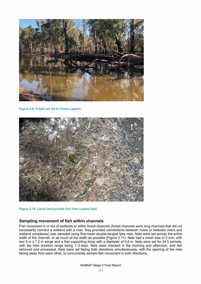
WetMAP Stage 3 Final Report
171
Figure 5.9: A fyke net set in Tarma Lagoon.
Figure 5.10: Larval and juvenile fish from a seine haul.
Sampling movement of fish within channels Fish movement in or out of wetlands or within forest channels (forest channels were long channels that did not necessarily connect a wetland with a river, they provided connections between rivers or between rivers and wetland complexes) was sampled using fine-mesh double-winged fyke nets. Nets were set across the entire width of the channel, or as much of the width as possible (Figure 5.11). Nets had a mesh size of 2 mm, with two 5 m x 1.2 m wings and a first supporting hoop with a diameter of 0.6 m. Nets were set for 24 h periods, with the total duration range being 1–3 days. Nets were checked in the morning and afternoon, and fish removed and processed. Nets were set facing both directions simultaneously, with the opening of the nets facing away from each other, to concurrently sample fish movement in both directions.

WetMAP Stage 3 Final Report
172
Figure 5.11: Double-winged fyke nets catching fish moving in a forest channel in Barmah Forest.
Fish processing Unless large numbers of fish were captured, all fish were identified to species and counted. When more than approximately 1000 fish were caught in a single net, numbers were assessed using gravimetric subsampling. In such cases, the number of each species was counted from three random subsamples of known weight. The number of fish per unit weight (from the subsamples) was then multiplied by the total weight of the catch to estimate the total number of each species. In some instances, rare or distinct fish (e.g. larger size) were removed from the sample before subsampling and counted separately. For both fyke and seine nets, a random sample of at least 25 fish of each species per site per sampling event were measured for length (caudal fork or total length, to nearest millimetre).
Zooplankton and chlorophyll a sample collection Zooplankton and chlorophyll a samples were collected at two sites during each visit to a wetland. Zooplankton were captured by filtering 20–50 L of water (collected from mid-depths) through a 50-μm sieve, after which they were stored in 70% ethanol. In the laboratory, organisms were identified as rotifers, copepods or cladocerans, following Shiel (1995), and counted under a dissecting microscope (Figure 5.12). Unless very few organisms were present, subsampling was used to make counting practicable. To do this, the entire volume of the sample was repeatedly halved until the sample could fit into a sorting tray. The organisms were dispersed evenly throughout the sorting tray, and then all organisms in a known area of the tray were counted. The resultant counts were multiplied by a factor accounting for the proportion of the original sample that was viewed (including the halving and counting of only a known area), to provide an estimate of the total number of organisms in the sample. The total number of zooplankton were then divided by the volume of water filtered to calculate the concentration of zooplankton in a sample. To estimate the abundance of phytoplankton, chlorophyll a concentrations were obtained by filtering a known volume of water through a Whatman™ 47 mm glass microfiber filter. The residue was later analysed by spectrometric determination (American Public Health Association, 2012).
Assessment of wetland size To calculate the size of wetlands at various times through the project, we used aerial imagery provided through Sentinel Playground (Sinergise Ltd, 2020). The extent of each wetland in each sampling period was drawn in Google Earth Pro, enabling calculation of the wetland area and perimeter. For very small wetlands, where the spatial resolution of aerial images alone was too coarse to determine the wetland area at the time of sampling, site photographs were used as a reference for wetland area, along with detailed site knowledge to estimate size.
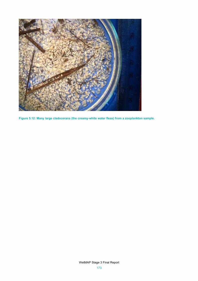
WetMAP Stage 3 Final Report
173
Figure 5.12: Many large cladocerans (the creamy-white water fleas) from a zooplankton sample.

WetMAP Stage 3 Final Report
174
Inundation extent and wetland productivity
KEQ 1: Is seasonal fish production (increase in the number of fish from late winter to summer) greater in wetlands that receive environmental water than in wetlands that do not?
SQ1: How does the spatial extent of wetland inundation during watering events affect food resources, fish recruitment and abundance within wetlands?
Methods Study sites Sampling was undertaken in seven wetlands: Margooya and Ducksfoot lagoons and Catfish Billabong in the MCMA region, and Bunyip Swamp, Cucumber Gully, Hut Lake and Tarma Lagoon in Barmah Forest in the GBMCA region, between spring 2018 and summer 2020 (Table 5.1).
Study design Our original intention was to answer KEQ 1 using a before–after–control–impact design to compare fish abundance in wetlands that received water with those that did not (but retained water). However, the wetlands that did not receive environmental water dried completely, which meant that this was not possible. Therefore, we adopted an alternative approach.
We investigated the impact of the spatial extent of wetland watering on food resources for fish, fish recruitment and fish abundance using three indicators (chlorophyll a, zooplankton and the abundance of the most commonly caught fish Carp Gudgeon). Three zooplankton classes (cladocerans, copepods and rotifers) were pooled. There was a high degree of correlation between Carp Gudgeon, native fish and all fish (r > 0.90), because Carp Gudgeon dominated the catch (see Appendix 12), which limited the number of fish categories that we could explore. We investigated within-year changes in abundance in relation to changes in wetland size for seven wetlands that did not receive water and those that experienced varying degrees of inundation. These wetlands were sampled during winter, early and late spring, and summer.
Data analysis Raw values representing density for each indicator (μg L–1 for chlorophyll a, count L–1 for zooplankton, and number of fish per fyke net) were adjusted to estimate an index of total abundance in wetlands. This was required to incorporate the impacts of changing wetland size on the number of organisms within wetlands between sampling periods. For example, if a wetland doubled in size, the density of organisms, as measured using our sampling techniques, would be expected to halve as organisms were redistributed throughout the wetland (assuming no increase in numbers through recruitment or immigration). Density values for chlorophyll a and zooplankton were multiplied by the area of the wetland in which they were obtained, at the time of sampling. Unfortunately, we do not have reasonable estimates of wetland volume, which would have provided a better estimate than using wetland area, so we relied on an assumed correlation between wetland area and volume for this adjustment. Mean Carp Gudgeon CPUE (catch-per-unit-effort; number of fish per net) was multiplied by the perimeter of the shoreline. Perimeter was chosen in this instance because nets most effectively catch fish moving along the shoreline, not those moving towards or away from shore (i.e. nets sample a length of shoreline rather than an area of the wetland).
We investigated the effect of the magnitude of wetland inundation on abundance by comparing the proportional change in estimated organism abundance against the proportional increase in wetland size, using Spearman’s rank correlation. Proportional change in the estimated abundance of organisms was calculated from the lowest capture rate early in the sampling season (late winter or early spring) to the highest capture rate (late in spring or in summer) in each year. This flexibility in timing was required (instead of fixed timing such as early spring to summer) to account for the variability in response times expected, based on the timing of watering, the behaviour of organisms and potential regional climatic variation affecting the timing of spawning. For example, fish spawning may begin earlier in the Mallee because it warms more quickly than wetlands further upstream on the Murray River. The proportional change in wetland size was calculated from the time immediately before watering began to the time of maximum inundation. Wetlands that did not receive water were assigned a proportional change of zero.
Results There may be a positive relationship between the increase in wetland area and the number of Carp Gudgeon produced in wetlands (Figure 5.13a; r = 0.67). However, the slope of this relationship is being largely driven by a single point representing a relatively large increase in inundation and a corresponding high increase in Carp Gudgeon numbers. This data point represents Ducksfoot Lagoon in 2019/20, following a managed and

WetMAP Stage 3 Final Report
175
extensive drawdown of the wetland (providing the opportunity for a large inundation event), and contrasts with the same wetland the previous year, which is close to the origin of the graph (zero inundation and a proportional increase in fish numbers of 1.4; Figure 5.13a).
Evidence of spawning by Carp Gudgeon was observed by the presence of larval fish in our seine hauls in all seven of our core wetlands. The spawning period was protracted, with some larval fish observed during late winter and spring, peak numbers in late summer and early autumn and several larval fish during late autumn. In addition, juvenile and adult Carp Gudgeon were also observed throughout our wetlands and sampling periods.
The early results show a potential positive relationship between the increase in wetland area and the abundance of chlorophyll a (Figure 5.13b; r = 0.61). Similar to the Carp Gudgeon result, this relationship is driven by few points (two in this case). Once again, Ducksfoot Lagoon in 2019/2020 stands out as having the greatest increase, Hut Lake the second greatest and Ducksfoot Lagoon in 2018/2019 the third greatest. These were the shallowest wetlands used in the investigation into productivity.
These data show no indication that zooplankton abundance is impacted by the increase in wetland area (Figure 5.13c; r = –0.25). One point, Tarma Lagoon stands out from the rest of the data set, with the largest increase in zooplankton abundance. This wetland was also high for Carp Gudgeon numbers, recording the second highest increase of the study wetlands.
Figure 5.13: Within-year proportional change in the abundance of Carp Gudgeon (panel a), chlorophyll a (Chl; panel b) and zooplankton (panel c) in relation to the proportional change in wetland size due to watering events, 2018–2020.

WetMAP Stage 3 Final Report
176
Discussion At this stage in WetMAP, we have documented support for our conceptual models relating to responses of fish production to wetland inundation. Positive correlations between the proportional increase in wetland size and proportional increases in Carp Gudgeon numbers and chlorophyll a concentration provide initial evidence that environmental watering benefits fish production. It is apparent that increases in Carp Gudgeon abundances were the result of successful spawning and subsequent recruitment to populations. This is based on observations that larval fish were present in all of the study wetlands throughout the sampling period and that there was no detectable immigration of Carp Gudgeon into wetlands (see Section 5.5.3). An increase in productivity and subsequent impacts on native fish communities is one of the main predicted impacts of implementing wetting/drying cycles in wetlands (Junk et al. 1989). Several studies have demonstrated a positive link between the area of dry land inundated and subsequent fish abundance in wetlands (Christensen 1993; Puckridge et al. 2000; Arthington et al. 2005). However, catchment-scale demonstrations of the effectiveness of this management tool are lacking, and we require more data to enable us to run statistical models before we can (statistically) demonstrate improvements to fish production in wetlands as a result of watering.
Further sampling would provide additional data to improve the statistical power to investigate fish production. Of interest is Margooya Lagoon, which will soon experience a managed, extensive drawdown. When this wetland is refilled, it will provide another large filling event in which the wetland more than doubles in size (similar to Ducksfoot Lagoon, which currently has a large degree of influence on the correlation coefficient). Given that increased variation in inundation levels will benefit our ability to detect impacts, the installation of a regulator at Catfish Lagoon may provide additional opportunities to sample more large inundation events (the potential to experience greater drawdown and watering events due to the regulator). Furthermore, the collection of additional data through time will allow us to run more complex models that may be able to account for some of the variation observed. For example, wetland and year can be included in models so that we can account for variability between wetlands and years resulting from several factors (e.g. bathymetry and aquatic vegetation).
The response of chlorophyll a, zooplankton and fish (larger increases with greater increases in inundation extent) may be impacted by predator–prey interactions between these groups. For example, large densities of Carp Gudgeon may reduce the density of zooplankton (a food source) despite high productivity due to large inundation events. However, at this stage of WetMAP, we have not been able to identify this as a driving factor. Given the rapid release of nutrients following flooding and the quick response of phytoplankton and zooplankton (within 6 days if temperature is high enough; Kobayashi et al. 2009), the timing of some of our sampling may have precluded our ability to observe short-term spikes in chlorophyll a and zooplankton. Fish diets can quickly shift to take advantage of post-flooding booms in productivity (Balcombe et al. 2005), and this, along with potential interactions between trophic levels, must continue to be considered for future planning and analyses.
Conclusions and future considerations The current findings have only been able to address these questions at a basic level.
KEQ 1: Is seasonal fish production (increase in the number of fish from late winter to summer) greater in wetlands that receive environmental water than in wetlands that do not?
We have not yet demonstrated differences in production between wetlands that receive environmental water and wetlands that do not, but the results so far provide some evidence to support this hypothesis.
SQ1: How does the spatial extent of wetland inundation during watering events affect food resources, fish recruitment and abundance within wetlands?
This question has not yet been answered, but the results for native fish and chlorophyll a are consistent with our conceptual model predictions.
Most of our original knowledge gaps relating to these questions still exist. Additional sampling through the next stage of WetMAP will be required before we could test for the effect of the extent of wetland inundation on the production of native fishes.

WetMAP Stage 3 Final Report
177
Wetland water regime
KEQ 2: Does water regime influence native fish species richness and abundance in wetlands?
SQ 2: How does wetland water regime influence native fish species richness and abundance in wetlands?
Methods Study sites We sampled 14 wetlands across northern Victoria in autumn 2019 (Table 5.1).
Study design To investigate the influence of wetland water regime on fish abundance and species richness, we compared results from three groups of wetlands with varying watering histories. Unfortunately, COVID-19 restricted our ability to collect data during autumn 2020, and although some sampling occurred it was in late May and early June and too late for inclusion in this report. Wetlands were grouped into three categories based on their water regime (Appendix 13):
Annual watering: These wetlands are in Barmah (Hut Lake, Tarma Lagoon, Cucumber Gully and Bunyip Swamp) and Gunbower forests (Black Swamp) and have occasional (twice per year to every second year) wetting and drying periods, receiving water from natural flooding and/or environmental water.
Natural wetting: These wetlands are in the Ovens River floodplain (RR8, RRx and Peechelba) and have frequent (several times per year) wetting and drying periods as a result of natural flooding.
Stable water levels: These wetlands are close to the Murray River, have regulated or unregulated connecting channels (Margooya, Ducksfoot and Sharpes lagoons, Catfish Billabong, Punt Paddock and Cameron’s Creek) and relatively stable water levels. Margooya Lagoon was drawn down early in 2016 and watered by mid-2016 and remained relatively stable since then.
Additional sampling We included an additional sampling technique to overcome issues in detectability of some species using the gear types described in Section 5.2. Species with a fast growth rate (notably Carp, Cyprinus carpio) may be too large by autumn to be captured using fine-mesh fyke nets (i.e. they cannot fit through the exclusion mesh that protects small fish in the net from predation). Therefore, we used coarse-mesh fyke nets (10 mm mesh size, 5 m x 0.6 m wing) to target larger fish, in addition to our fine-mesh fyke nets. These nets were deployed in the same manner as the fine-mesh fyke nets, but did not have the exclusion mesh, so they would trap larger species.
Data analysis We used one-way analysis of variance (ANOVA) or Kruskal–Wallis tests (as a non-parametric alternative when ANOVA test assumptions were not met) to investigate whether density (catch per net from fine-mesh fyke nets) and/or species richness (from fine- and coarse-mesh fyke and seine nets) differed between wetlands for the three watering classifications. Separate tests were run for native and non-native fishes. Black Swamp was not included in the density analyses because it was severely drawn down from its recent maximum extent, but not yet to the point when high levels of mortality would have decreased fish numbers. This resulted in large numbers of fish concentrated in a small area, with total catches being an order of magnitude greater than at any other wetland in autumn, and comparable with the highest catch per net observed in summer across all wetlands.
Results We caught a total of 58,733 native fish across all wetlands sampled in autumn 2019 (Appendix 14). Catches were dominated by Carp Gudgeon (n = 57,535). We caught a total of 20,937 non-native fish, which were dominated by Eastern Gambusia (Gambusia holbrooki; n = 23,334). For both native and non-native species, wetlands in the natural wetting grouping had the highest mean density (native = 1724.1 fish per net; non-native = 996.1 fish per net), followed by stable water level (native = 597.3 fish per net; non-native = 228.5 fish per net) and annual watering (native = 496.8 fish per net; non-native = 94.1 fish per net; Figure 5.14). However, no significant differences were detected (native fish: Chi-square = 4.9, df = 2, p = 0.088; non-native fish: Chi-square = 5.7, df = 2, p = 0.059). For native species, mean species richness was highest at stable water level wetlands (S = 3.8), followed by natural wetting wetlands (S = 3) and annual wetlands (S = 2.6). For non-native species, mean richness was highest at annual watering wetlands (S = 3.6), followed by stable water level

WetMAP Stage 3 Final Report
178
wetlands (S = 2.7) and natural wetting wetlands (S = 2). However, similar to density, no significant differences were detected in species richness between wetland groups (native: F = 0.91, df = 2, p = 0.43; non-native: F = 2.71, df = 2, p = 0.11) (Figure 5.14).
Figure 5.14: Mean values (squares) of fish density (left panel) and species richness (right panel) for native and non-native fish at each wetland type, along with the raw values for each wetland (small circles).
Discussion At this stage, we do not have enough data (and thus statistical power) to determine how native and non-native fish communities are impacted by wetland water regimes. Despite this, we have observed promising relationships that support our conceptual models.
There may be a relationship between the density of fishes in autumn and the wetland water regime. The observed densities of native and non-native fishes were higher in wetlands that experienced a natural wetting regime than in those that were inundated less frequently (annual watering and stable water level). However, none of these results was statistically significant, which is not surprising given the variability in fish densities within groups and that we only have one year of data in these analyses. Despite this, these early trends provide some support for our conceptual models, and continued monitoring in these types of wetlands is warranted. Beesley et al. (2014a) found that native fish responded best to frequent inundation of wetlands (occurring annually, or more often), whereas non-native fish species generally did better with less frequent inundation events. During inundation of terrestrial areas, fish diets can shift (Wantzen et al. 2002; Pool et al. 2017) to take advantage of the boom in primary productivity and the release of nutrients after inundation of previously dry areas (Kobayashi et al. 2015). In wetlands that are often inundated and then allowed to draw down (such as at our naturally inundated wetlands), fish will have frequent access to terrestrially derived resources. Recruitment, and hence fish density, is likely to be greater when the timing of inundation coincides with ideal overall conditions for spawning (King et al. 2009; Górski et al. 2011; Beesley et al. 2014b). A natural wetting regime typically involves numerous inundation events occurring during winter and early spring, which coincides with spawning periods for many of our native wetland fish species. In addition, autumn densities of native fishes have possible effects on spawning in spring, because higher densities of native fish (particularly Carp Gudgeon) in wetlands during autumn may provide a larger standing stock of fish available for spawning when temperatures increase in spring (see Section 5.5.3).
At this stage of WetMAP, we have not demonstrated an impact of wetland water regime on native species richness. Although values appear higher for wetlands experiencing a stable water level due to long-term connections with the Murray River, circumspection is necessary as these results are based on a single year, there is a large amount of variation in the data, and additional sampling is required to investigate the relationship. Several authors have found higher fish species richness at wetlands with better hydrological connectivity (Snodgrass et al. 1996; Baber et al. 2002; Henning et al. 2007; Lasne et al. 2007), because it is

WetMAP Stage 3 Final Report
179
more likely that fish will encounter and enter these wetlands. Furthermore, the density and composition of fish in the source water will also affect the outcome of any watering event (Snodgrass et al. 1996), because rarer or less abundant species will be less likely to enter a wetland. In the Murray–Darling Basin, many small-bodied wetland specialist species are currently severely restricted relative to their historic distributions (Lintermans 2007) and would not be present in the source water to encounter and colonise our study wetlands even if conditions were favourable. Regional influences on the number of species available to colonise our study wetlands can impact our ability to determine the influence of water regime on species richness. For example, wetlands with natural wetting regimes are rare, and all the ones we sampled occurred in the Ovens River catchment. This means there that we are at risk of conflating the distribution of species in the Ovens River catchment with the influence of natural wetting regimes. There are two approaches that can alleviate this issue. The first is to have a much broader array of wetlands sampled across the landscape and over a longer period. The second is an adaptive management approach in which environmental water is used to mimic the natural water regime in other regions.
Similar to native fish species, we have not demonstrated an impact of water regime on non-native species richness. We did observe lower levels at the three wetlands in the natural wetting category, somewhat in concordance with Beesley et al. (2014a) who found that non-native fish density responded poorly to frequent watering events. Determining water regimes that negatively impact non-native species while benefiting native species would provide a strong rationale to water managers to use environmental water to create these water regimes.
The use of autumn sampling data to investigate the impacts of wetland water regime in WetMAP will allow for the inclusion of data from The Living Murray initiative (TLM) to potentially increase our statistical power. TLM uses comparable methods, and data collection has occurred at many wetlands over many years. We recommend that the next stage of WetMAP collate TLM data into a single, consistent database for inclusion in WetMAP analyses. This will also require determining the water regimes for these wetlands over an extended period.
Conclusions and future considerations The current findings have only been able to address these questions at a very basic level.
KEQ 2: Does water regime influence native fish species richness and abundance in wetlands?
SQ 2: How does wetland water regime influence native fish species richness and abundance in wetlands?
These questions have not been answered yet. However, there is evidence that wetlands with a natural water regime (largely unaffected by river regulation) have higher fish densities and native species richness.
Despite support for our conceptual models, our original knowledge gaps relating to these questions still exist. The inclusion of TLM data may provide additional statistical power to address these questions, along with the potential to investigate the effect of more specific watering classifications on native species richness and abundance in wetlands. An adaptive management approach in which wetlands in other regions experience a more natural wetting regime could also improve our ability to determine the impact of environmental watering on native species richness and abundance in wetlands.

WetMAP Stage 3 Final Report
180
Immigration and emigration of native fishes
KEQ 3: Do environmental water events provide opportunities for fish to move between wetlands and rivers?
SQ 3: Does connectivity of wetlands with their source water facilitate the immigration of adult fish or dispersal of juvenile fish?
Methods Study sites We sampled the connecting channels of wetlands with a direct connection to the Murray River (two sites) and forest channels (six sites; Figure 5.8; Table 5.2). Forest channels were long channels that did not necessarily connect a wetland with a river, they provided connections between rivers or between rivers and wetland complexes.
Study design We used two approaches to monitor whether watering events provided wetland connectivity for the immigration and emigration of fishes. The first looked at whether there was directional movement of two life stages (juveniles and adults) in connecting channels (those in forest complexes and those directly connecting wetlands with the Murray River). The second looked at whether the abundance of adult fish in wetlands was affected by the immigration of fish from rivers. These approaches focused on the two most abundant and spatially distributed species in this study (Australian Smelt and Carp Gudgeon). Australian Smelt <30 mm in caudal fork length (CFL) were considered juveniles (Tonkin et al. 2008), and those ≥35 mm CFL were considered adults (based on size distributions from the current study; Milton and Arthington 1985). Carp Gudgeon <25 mm CFL were considered juveniles (Beesley et al. 2012), and those ≥30 mm CFL were considered adults (Unmack 2000). These discontinuous length categories result in some fish that were not considered juveniles or adults and were excluded from life-stage analyses. This was required to decrease the chance of fish being incorrectly assigned to a life stage.
Direction of movement Bi-directional netting over 24-h periods (see ‘Sampling movement of fish within channels‘ in Section 5.2) in September 2019 was completed within forest channels (Figure 5.11) to investigate whether adult fish move with or against the flow of water in forest systems. Sampling within forest channels was limited to a few days in winter due to the timing of the opening of regulators. For this set of samples, we could not determine whether fish were moving into or out of wetlands, because sampling locations were not associated with individual wetlands. Instead, these locations were in larger forest channels close to the Murray River or Gunbower or Budgie creeks, which flowed into a diffuse system of channels and wetlands within the forest.
Bi-directional netting over 24-h periods was also used within channels directly connecting wetlands to the Murray River (i.e. Margooya and Ducksfoot lagoons) to determine whether juvenile and adult fish were immigrating into wetlands or emigrating from wetlands throughout spring in 2018 and 2019 (Table 5.2). In these cases, we investigated whether fish were moving in or out of wetlands. Sampling finished in November because the regulators were closed thereafter.
Change within wetlands Fyke and seine netting were used to investigate changes in the density and abundance of adult fishes within wetlands as a result of immigration into wetlands during watering events. We used a before–after control–impact design, with pre- and post-watering results collected during autumn and August 2019. Four impact wetlands (Hut Lake and Catfish, Margooya and Tarma lagoons) received water during winter, resulting in connections to rivers that could allow fish to enter in source waters, while three control wetlands (Bunyip Swamp, Cucumber Gully and Ducksfoot Lagoon) did not receive water and remained disconnected. Sampling was undertaken prior to native fish spawning so that recruitment would not confound results.

WetMAP Stage 3 Final Report
181
Data analysis
Direction of movement
Forest channels
A generalised linear model was used to test for differences in adult Australian Smelt movement relative to the flow of water in forest channels (i.e. were fish moving with the flow or against the flow in channels?). The model included the number of fish captured (response variable), movement direction in relation to flow (with or against) and an offset for effort (natural logarithm of the number of 24-h periods sampled). Channel could not be included as a predictor due to the limited amount of sampling (one sampling event at each of six sites). We assumed that the count data followed a negative binomial distribution and assessed the appropriateness of this assumption with posterior estimates of the dispersion parameter. This model was run using the statistical package R v3.2.5 (R Development Core Team 2015) and the MASS package (Venables and Ripley 2002). A model for Carp Gudgeon could not be completed due the small number of fish captured at five of six sites. Therefore, the modelling was only undertaken for Australian Smelt. Modelling for juvenile Australian Smelt was not completed because very few (n = 9) were captured in forest channels at this time of year.
In or out of wetlands
Generalised linear models (one for each species/life-stage combination) were used to test for differences in fish movement in and out of wetlands that had a direct connection with the Murray River (Ducksfoot and Margooya lagoons; i.e. were fish moving in or out of wetlands?). Three of the four models (juvenile Carp Gudgeon and adult Carp Gudgeon and adult Australian Smelt) were successful and included the number of fish captured (response variable), direction and channel (and the direction*channel interaction), month (September, October or November), and an offset for effort (natural logarithm of the number of 24-h periods sampled). We assumed that the count data followed a negative binomial distribution and verified the appropriateness of this assumption with posterior estimates of the dispersion parameter. These models were run using the statistical package R v3.2.5 (R Development Core Team 2016) and the MASS package (Venables and Ripley 2002). An acceptable generalised linear model could not be generated for juvenile Australian Smelt. As an alternative, we used a paired Wilcoxon test to investigate whether more juvenile Australian Smelt moved out of wetlands than in. This test included the mean number of fish per 24-h period (per wetland, month and year) as the dependent variable and fish direction (in and out) as the predictor variable.
Change within wetlands
Generalised linear models were used to test for differences in adult fish populations resulting from watering events providing connection to wetlands during late winter and early spring. Two models were run for each species (Carp Gudgeon and Australian Smelt), investigating changes in abundance and density. The models included the total number of fish captured in each wetland and each sampling event (response variable), a treatment (connected or not) by time (before and after connection) interaction, and an offset for effort. The offset varied depending on the analysis (fish density or abundance). For fish density, the offset was the natural logarithm of the number of sites sampled in the wetlands (with the catch per net reflecting fish density). For fish abundance, the offset was the number of sites relative to the perimeter of the wetland (reflecting fish abundance in the wetland, assuming that nets sampled a distance of shoreline rather than an area of the wetland). Wetland was not included as a factor in the models because it did not improve the models and in some cases resulted in invalid models. We assumed that the count data followed a negative binomial distribution and assessed the appropriateness of this assumption with posterior estimates of the dispersion parameter. These models were run using the statistical package R v3.2.5 (R Development Core Team 2016) and the MASS package (Venables and Ripley 2002).
Results Direction of movement
Forest channels
Over 18,300 Australian Smelt and Carp Gudgeon were captured moving in forest wetland channels. These included 2502 Australian Smelt (9 juveniles, 2363 adults and 130 undetermined) and 15,840 Carp Gudgeon (1846 juveniles, 9024 adults and 4970 undetermined). A full list of species caught is included in Appendix 15. Most of the adult Australian Smelt (82%) were moving against the flow of water, 15% were moving with the flow of water and less than 3% were in one channel with little to no flow (Green Swamp), which was not included in the model. Significantly more Australian Smelt moved against the flow than with it (z = 2.98;

WetMAP Stage 3 Final Report
182
p = 0.003; Figure 5.15). Depending on the sample site, fish moving against the current were moving into or out of forest complexes. Almost all (99%) of the Carp Gudgeon were captured at one site in the Green Swamp channel in Gunbower Forest, where there was little to no flow.
Figure 5.15: Generalised linear model predictors of the direction of movement of adult Australian Smelt relative to the flow of water in forest channels, September 2019.
In or out of wetlands
Almost 99,000 Australian Smelt and Carp Gudgeon were captured moving in channels connecting wetlands directly to the Murray River during spring. These included 44,452 Australian Smelt (44,051 juveniles, 378 adults and 23 undetermined) and 54,474 Carp Gudgeon (6935 juveniles, 31,824 adults and 15,715 unknown). A full list of species caught is included in Appendix 15.
More adult Australian Smelt were captured moving out of wetlands (57%) than in (43%) from September to November, but this result was not significant (z = 1.21; p = 0.23; Figure 5.16a). However, significantly fewer adult Australian Smelt were moving in either direction during November compared with September and October (z = –2.52; p = 0.012; Figure 5.16a). In contrast to adults, significantly more juvenile Australian Smelt were captured moving out of wetlands (99%) than in (1%) during spring (p = 0.039; Figure 5.16c). The use of a Wilcoxon test meant that we could not test for differences in the number of juvenile Australian Smelt moving out of wetlands between months. However, the observed rates were: 0.3, 1800 and 923 wetland–1 d–1 in September, October and November, respectively.
Similar numbers of adult Carp Gudgeon were captured moving in (50.3%) and out (49.7%) of wetlands over the study period (z = 1.45; p = 0.15; Figure 5.16b). However, significantly more adult Carp Gudgeon were moving in either direction during October (z = 2.36; p = 0.019; Figure 5.16b) and November (z = 3.60; p < 0.001; Figure 5.16b) compared with September. In contrast to adults, significantly more juvenile Carp Gudgeon were moving out of wetlands (80%) than in (20%; z = 2.78; p = 0.005; Figure 5.16d). The trend was similar between months (September to November), with no significant differences in the number moving detected between months (z = –0.88 and –0.42; p = 0.380 and 0.967 respectively; Figure 5.16d).

WetMAP Stage 3 Final Report
183
Figure 5.16: Generalised linear model predictors (panels a, b and d) and a box plot (panel c) of the direction of movement (in or out of wetlands) of Australian Smelt and Carp Gudgeon in wetland connecting channels in spring 2018 and 2019.
Change within wetlands We caught a total of 890 adult Australian Smelt and 5939 adult Carp Gudgeon in the seven wetlands before and after watering events provided connectivity to impact wetlands during winter and early spring. The number of adult Australian Smelt was similar between the pre- (n = 41) and post-watering (n = 42) periods in the control wetlands, but increased from 24 to 783 in the impact wetlands. Abundance and density of Australian Smelt increased significantly at the impact wetlands relative to the control wetlands (z = 3.74; p < 0.001 for abundance and z = 2.64; p = 0.008 for density; Figure 5.17). In contrast, the number of adult Carp Gudgeon captured decreased between the pre- and post-watering periods at control (2634 to 521) and impact (2273 to 511) wetlands. There was no significant effect of watering on Carp Gudgeon density (z = 0.11; p = 0.912; Figure 5.17) or abundance (z = 1.88; p = 0.060; Figure 5.17) detected at impact wetlands relative to control wetlands.

WetMAP Stage 3 Final Report
184
Figure 5.17: Generalised linear model predictors of the change in density (top panels) and abundance (bottom panels) of Australian Smelt and Carp Gudgeon in wetlands that were hydrologically connected with the Murray River (impact) relative to those that were not (control) in 2018 and 2019.
Discussion To our knowledge, this study is the first to demonstrate changes in the abundance and density of adult small-bodied fishes in wetlands as a result of immigration and the subsequent dispersal of juvenile fish to the Murray River. Immigration and emigration of fishes to and from wetlands is a process that allows fish inhabiting rivers to access productive and complex wetland habitats for spawning, recruitment and better feeding opportunities (Junk et al. 1989). It also provides river access to potentially high densities of wetland fishes for dispersal and resultant nutrient transfer to rivers following recruitment (Winemiller and Jepsen 1998). Knowledge of how native fishes use connectivity between wetlands and rivers, and of the effectiveness of environmental flows in creating connectivity, is required to help mitigate the impacts of river regulation.
Australian Smelt Environmental watering of wetlands, connecting them to the Murray River, resulted in the immigration of adult Australian Smelt to wetlands. Density and abundance of Australian Smelt increased in our study wetlands that received water during winter 2019 relative to those that did not receive water. This demonstrated that adult fish immigrated into wetlands during watering. Although wetland connectivity was facilitated for all of our impact wetlands during late winter, some also received water as early as July and this study has not determined whether immigration occurs throughout winter. However, we do have some very recent information indicating that adult Australian Smelt will immigrate into wetlands in late autumn if connectivity is provided (unpublished data).

WetMAP Stage 3 Final Report
185
Adult Australian Smelt also moved in connecting channels during environmental watering events during early spring. These fish largely moved against the current in channels within forest wetland complexes. This did not necessarily result in the movement of fish into wetlands; at three of five sites where water was flowing, the greatest amount of movement was towards the Murray River. At the other two locations, there was greater movement into Gunbower Forest from Gunbower Creek and to Hut Lake from Budgie Creek. Given that evidence of Australian Smelt spawning (i.e. the capture of larval fish) was observed in this study as early as mid-September, some of the fish captured in the forest connecting channels could have been post-spawning adults moving towards rivers. However, the largest numbers of larval Australian Smelt in this study were captured in wetlands in late October and early November, which coincides with the maximum larval catches reported by Humphries et al. (2002), and we speculate that most Australian Smelt would not have spawned by early spring, when the forest channel movement was observed. In addition, some of the Australian Smelt captured in forest connecting channels were ripe females and had not spawned yet (unpublished data). This species is known to have an extended spawning period: a study in two rivers over four spawning seasons recorded larval fish from August to April (Humphries et al. 2002), and ripe female fish have been observed as early as July (Milton and Arthington 1985). Our findings provide early evidence that flows in forest channels facilitate the movement of Australian Smelt in September and their distribution in the landscape, but not necessarily their immigration to wetlands.
This study did not detect a difference in the number of adult Australian Smelt moving in or out of wetlands through channels directly connecting wetlands to the Murray River. This result appears to contradict the results obtained from forest channels. However, sampling within these wetland channels began in September at least 1 month after the opening of regulators, in contrast with the forest channels, in which sampling occurred during the short period when the regulators were open (within days of opening). Along with the findings of increased abundance and density of Australian Smelt in the wetlands with direct connections due to winter watering, this indicates that adult immigration into wetlands may occur soon after connectivity is reinstated and does not occur continuously over an extended period. In addition, fewer adult Australian Smelt were captured in these channels later in the sampling period (November), which followed the peak spawning period of Australian Smelt and may reflect a decrease in adult Australian Smelt abundance within wetlands as a result of post-spawning mortality or unobserved emigration from wetlands. Conallin et al. (2011) caught 147,848 adult Australian Smelt moving between rivers and wetlands between August and November. However, a significant effect was only detected at one of their six study wetlands, in which 26,088 fish were captured moving out and 3648 fish moving in. Their study wetlands had also been connected to the Murray River for some time, and flow conditions were stable during sampling.
Juvenile Australian Smelt dispersed from wetlands with direct connections with the Murray River when connectivity existed in mid- to late spring. We observed a net movement of over 43,000 juveniles out of two wetlands into the Murray River in October and November, averaging almost 1700 fish per day per wetland. However, given our study wetlands were disconnected from the Murray River following the last November sampling events, we cannot determine how long this emigration period may last. We can only infer that this process will continue, at least into early summer, based on similar levels of emigration between October and November (i.e. there was no indication that the emigration rate was decreasing by our latest sampling times in November). Lyon et al. (2010) also found large numbers of Australian Smelt moving out of wetlands during late November; however, they did not report on the size or life stage of these fish, so it is unknown whether this was the result of the emigration of juveniles. Regardless, by March, there was no clear direction of movement detected (Lyon et al. 2010), indicating that the process had finished. This emigration process has the potential for considerable nutrient transfer from wetlands to the Murray River because, despite the small size of juvenile Australian Smelt, large numbers were emigrating, and the process can occur across the landscape (Kwak 1988).
Based on the findings of this study, we have identified some ways that Australian Smelt use wetlands. Adult Australian Smelt immigrate into wetlands during mid- to late winter when connectivity between wetlands and rivers or creeks exists, increasing their abundance and density within wetlands. However, the timing of this process remains uncertain because it may also occur in autumn and early winter, and it requires more thorough investigation, targeting watering events at various times of year. Australian Smelt then spawn in wetlands during spring, resulting in peak catches of larval fish in mid- to late spring in northern Victoria. Finally, juvenile Australian Smelt emigrate from wetlands in large numbers to the Murray River in mid- to late spring if connectivity is provided.
Carp Gudgeon Based on adult Carp Gudgeon abundance within wetlands, environmental watering of wetlands, providing connectivity with the Murray River, did not appear to result in immigration to wetlands. However, the change in abundance in the impact wetlands relative to the control wetlands (p = 0.06) was close to the statistically significant value (p = 0.05). This finding warrants additional sampling to increase our statistical power. In contrast to Australian Smelt, the density and abundance of Carp Gudgeon decreased between the periods

WetMAP Stage 3 Final Report
186
before and after winter watering in control and impact wetlands. This was not the result of emigration of fish from wetlands, because the decline also occurred in our control wetlands (those that were not connected to other waterbodies). This decline could be the result of over-winter mortality of Carp Gudgeon or a decrease in catch efficiency. However, the decrease in catch was observed in both of our capture techniques (passive fyke nets and active seine nets), indicating that catch efficiency of fish inhabiting the littoral zone of the wetlands was not affected.
This study did not demonstrate directional movement of adult Carp Gudgeon in forest channels or in channels directly connecting wetlands to the Murray River. This provides evidence that immigration does not play a significant role in determining the spawning stock of adult fish in permanent wetlands. However, there is limited evidence that adult Carp Gudgeon migrated out of one of these study wetlands in large numbers during a subsequent summer watering event that followed the contraction of the wetland (Cornell et al. 2019). Similar to our findings, Conallin et al. (2011) did not record any difference in the directionality of Carp Gudgeon movement during late winter and spring (August to November). However, Lyon et al. (2010) recorded more Carp Gudgeon moving into wetlands than out during late spring and late summer, and the reverse during late autumn. More sampling of connection events at additional times of year is required to investigate the role of timing on the possible emigration of adult fish.
Juvenile Carp Gudgeon dispersed from wetlands with direct connections with the Murray River when connectivity existed in spring. We observed a net movement of almost 4200 juvenile Carp Gudgeon out of two wetlands into the Murray River during this study, averaging around 170 fish per wetland per day from September to November. We hypothesise that the process of emigration of juvenile Carp Gudgeon can continue through summer, based on the continued spawning of the species through late spring and summer and the large number of juvenile fish captured trying to exit Margooya Lagoon during a watering event in February 2019 (Cornell et al. 2019). Although fewer juvenile Carp Gudgeon were detected emigrating from wetlands during spring than Australian Smelt (around 10%), we speculate that this process can occur over a longer period (based on the Carp Gudgeon’s protracted spawning period; Vilizzi and Tarkan 2016), and as such can represent significant nutrient transfer from wetlands to rivers, particularly when both species are considered together. Indeed, the movement of fish between off-channel and main stem areas can be an important mechanism for the transfer of carbon (Roach et al. 2009). However, additional sampling of connection events at other times of year is required to investigate the how long these fish continue to emigrate from wetlands.
Based on the findings of this study, we have identified some ways that Carp Gudgeon use wetlands. In wetlands that do not dry completely or result in a die-off of fish due to other factors (e.g. water quality), we expect that a standing stock of Carp Gudgeon remain resident in wetlands. These are not significantly increased by the immigration of new adults during winter watering events. The spawning of the standing stock of Carp Gudgeon occurs over an extended period in permanent/semi-permanent wetlands (Vilizzi and Tarkan 2016), producing large numbers of larval fish, resulting in recruitment to the population. Subsequent connection of wetlands to the Murray River (September to February) results in juvenile Carp Gudgeon emigrating from wetlands to the less productive river system. Given that two of our study wetlands dried during the summer of 2020, we will be able to begin investigating the colonisation of Carp Gudgeon through the immigration of fish into wetlands and the time it takes for populations to build.
Conclusions and future considerations The current findings have answered our initial questions relating to the immigration and emigration of native fishes to and from wetlands.
KEQ 3: Do environmental water events provide opportunities for fish to move between wetlands and rivers?
Yes, we have demonstrated that there is directional movement of fish in wetland channels when environmental watering events provide connections with wetlands.
SQ 3: Does connectivity of wetlands with their source water facilitate the immigration of adult fish or dispersal of juvenile fish?
The provision of environmental water during winter resulted in the immigration of adult Australian Smelt into wetlands (prior to spawning and recruitment to the populations). This resulted in an increase in the number and density of fish within the wetlands. However, a similar result for Carp Gudgeon was not detected. Furthermore, the continued connectivity throughout spring provided extended periods of time for the dispersal of thousands of juvenile Australian Smelt (October and November) and Carp Gudgeon (September through November) into the Murray River.

WetMAP Stage 3 Final Report
187
Additional knowledge gaps can be filled with further investigations relating to this subject. First, we do not know the time frame when adult Australian Smelt will migrate into wetlands. Does time of year play a role? This can be investigated by targeting specific watering events during specific months in summer, autumn and winter (if watering events occur during these periods). Second, we do not know the duration of the immigration of adult Australian Smelt into wetlands. Given no movement was detected in channels directly connecting wetlands to the Murray River (which were sampled more than a month after regulators were initially opened) and movement was detected in the forest channels (which were sampled immediately after regulators were opened), we hypothesise that the response of Australian Smelt is immediate, and that once fish resident in the area around the channel have moved, their immigration slows or stops. Third, the dispersal of juvenile Australian Smelt and Carp Gudgeon continued (with no indications of decreasing rates) out of Ducksfoot and Margooya lagoons until regulators were closed in November, and we do not know how long their dispersal can be maintained. Additional sampling is required to attempt to address this knowledge gap. Finally, we do not know whether the direction of flow within connecting channels with a direct connection to the Murray River impacts the rate of fish movement. Thus far, water was always flowing into Ducksfoot Lagoon during channel sampling and the direction of flow to and from Margooya has varied and was often negligible. Future sampling efforts can be made to quantify the impact of flow direction and velocity on the movement of fishes.
Monitoring the persistence of Murray Hardyhead
KEQ 4: Do Murray Hardyhead persist in saline wetlands where environmental water is effectively used to maintain wetland salinity levels within the range required for successful spawning and recruitment?
Methods Study sites We sampled five wetlands for the presence of Murray Hardyhead during autumn each year from 2017 to 2019 (Figure 5.8, Table 5.3). Annual monitoring was planned for autumn 2020 but was not completed due to COVID-19 restrictions.
Monitoring design We monitored the persistence of Murray Hardyhead at several wetlands with different electrical conductivity (EC) levels, where the species had previously occurred. EC was recorded at each wetland at the time of sampling in autumn. Additional, longer-term EC data were collected by CMA staff to provide information on the influence of environmental water on EC in saline wetlands.
Fish sampling The approach differed from the generalist species methods due to the rarity of Murray Hardyhead and the need to minimise unnecessary disturbance to these threatened populations. A combination of survey equipment was used at each site, and the sampling dates and sampling intensity are outlined in Table 5.3.
A large seine net (24 m x 2 m x 8 mm) was deployed in the same manner as the small seine net described in ‘Sampling fish within wetlands‘ in Section 5.2. A small seine net (7 m x 1 m x 2 mm) was deployed by carrying it out approximately 15 m towards the centre of the wetland. It was then strung out between two operators (parallel to shore) and hauled back slowly to the shore, ensuring that the lead-line remained as close to the substrate as possible, and the float-line remained at the surface. On approach to the shore, the operators gradually moved together and, on reaching the shore, closed the net. The net was then hauled in and its contents removed on the shore of the wetland.
Fyke nets were set at randomly selected sites within each wetland at approximately 1.0–1.5 m depth, for a minimum overnight soak time of 12 h. Fyke nets had dual wings 8.9 m x 1.2 m, a first supporting hoop with a diameter of 0.5 m, and a stretched mesh size of 2 mm.
To minimise disturbance to populations, fyke nets were only deployed in each lake if the combined catch from hauls of large and small seine nets (done on the first day) did not capture more than 20 adult Murray Hardyhead. If fyke nets were required to be set, and fewer than 20 adult Murray Hardyhead were captured during the first night, the fyke nets were set for an additional night.
Captured fish were pooled by method and identified to species and counted, and Murray Hardyhead were measured for CFL (to the nearest millimetre). When large numbers of Murray Hardyhead were caught, up to 50 fish were chosen randomly and measured for CFL. Native species were released back to the site of capture, while non-native species were anaesthetised by placing them in a solution of water and clove oil (40 mg/L) for 10 minutes.

WetMAP Stage 3 Final Report
188
Table 5.3: The location, timing, gear type and effort for the investigation into the persistence of Murray Hardyhead between 2017 and 2019. The sample date is the first day of each trip if the trip was over multiple days.
Waterbody Date Large seine net Small seine net Fyke net
2017
Round Lake 18 September 2 2 4
2018
Lake Elizabeth 17 April – 1 8
Brickworks Lagoon 26 March 2 2 8
Round Lake 28 March 2 2 8
Lake Koorlong 1 March 2 2 12
2019
Lake Elizabeth 29 April 2 2 8
Round Lake 29 April 2 2 –
Lake Hawthorn 30 April 2 2 8
Brickworks Lagoon 30 April 2 2 8
Water quality and wetland watering At the time of fish sampling, EC (standardised to 25ºC µS cm–1) was recorded at survey sites 0.2 m below the water surface using a YSI handheld water quality meter. In addition, EC readings were supplied by the NCCMA in 2020 for Lake Elizabeth (between April 2014 and April 2020) and Round Lake (between September 2016 and April 2020). Readings were taken using a YSI conductivity meter, fortnightly during watering events and monthly at other times of year. Corresponding lake height readings (from a water level gauge) were recorded at most instances when an EC reading was taken. The dates of environmental water delivery and the amount delivered to these two wetlands was also supplied by the NCCMA. Similar data were not available for the other wetlands monitored.
To investigate the relationship between EC and wetland watering, we graphed EC through time at Lake Elizabeth and Round Lake and overlaid the duration of environmental water delivery events. We also fitted a linear regression between EC and lake height and calculated an R2 value. This regression tested the mechanism behind EC change in relation to wetland watering, that is, that as lake height increases, EC decreases due to dilution.
Results Murray Hardyhead sampling A total of 1745 Murray Hardyhead were caught at four wetlands on five occasions. No Murray Hardyhead were caught at Round Lake in 2017 or 2018, but 28 were captured at Round Lake in 2019 using seine nets alone (a relatively high catch, exceeding our 20 fish target, meaning that fyke nets were not required; Table 5.4). No other fish species were caught at Round Lake in 2019. Catches of Murray Hardyhead at Lake Elizabeth also increased between samples, with 34 caught in 2018 and 865 caught in 2019 (Table 5.4). No fish were captured in Lake Hawthorn (where they had previously been present), despite seine hauls being undertaken and fyke nets being set for two nights (Table 5.4). Two Murray Hardyhead were captured in Brickworks Lagoon (both in 2019), along with relatively high numbers of other species, native and non-native (Table 5.4).
Murray Hardyhead caught at Lake Koorlong were not measured but estimated to range between 20 and 50 mm. Murray Hardyhead captured at Lake Elizabeth in 2018 ranged between 25 and 35 mm, while those caught in 2019 were predominantly 40 to 50 mm CFL, ranging from 27 to 78 mm CFL (Figure 5.18). Likewise, the length range of Murray Hardyhead captured at Round Lake in 2019 was 29 to 64 mm CFL. The two individuals of the species captured from Brickworks Lagoon were 28 and 29 mm CFL.

WetMAP Stage 3 Final Report
189
Table 5.4: Catch per species and electrical conductivity (EC; µS cm–1) in wetlands targeted for Murray Hardyhead in WetMAP. Catches are pooled for all gear types, and the sample date is the first day of each trip if the trip was over multiple days.
Waterbody Date EC Species Total
Round Lake 2017 18 September 32,600 Flat-headed Gudgeon 1
Gambusia 23
Round Lake 2018 28 March 35,800 Gambusia 3
Round Lake 2019 29 April 36,300 Murray Hardyhead 28
Lake Elizabeth 2018 17 April 79,000 Murray Hardyhead 34
Gambusia 4
Lake Elizabeth 2019 29 April 15,340
Murray Hardyhead 865
Carp 1
Gambusia 15
Flat-headed Gudgeon 1
Lake Koorlong 2018 1 March 6,620
Murray Hardyhead 816
Carp Gudgeon 69
Gambusia 5,370
Brickworks Lagoon 2018 26 March 3,500
Australian Smelt 109
Flat-headed Gudgeon 4
Carp Gudgeon 14,068
Gambusia 8
Brickworks Lagoon 2019 30 April 5,930
Gambusia 2,241
Carp Gudgeon 2,945
Murray Hardyhead 2
Lake Hawthorn 2019 30 April 74,100 No fish

WetMAP Stage 3 Final Report
190
Figure 5.18: Length–frequency distributions for Murray Hardyhead caught at Lake Elizabeth in 2018 (panel a) and 2019 (panel b) and at Round Lake in 2019 (c).
Water quality and wetland watering EC varied through time at Lake Elizabeth and Round Lake, with decreases associated with environmental watering events (Figure 5.19). At Lake Elizabeth, EC ranged between 20,100 and 83,400 µS cm–1 (n = 80). There were 19 separate environmental watering events, with total delivery volumes of between 100 and 700 ML. Spring EC readings exceeded 45,000 µS cm–1 in November 2015, early October 2018 and October 2019. At Round Lake, the EC ranged between 24,600 and 49,342 µS cm–1 (n = 36; Figure 5.19). There were 11 separate environmental watering events, with total delivery volumes of between 80 and 300 ML. Spring EC readings did not exceed 45,000 µS cm–1 (Figure 5.19). Across all wetlands, EC at the time of sampling ranged between 3500 and 74,100 µS cm–1 (Table 5.4). Linear regressions between water height and salinity at Lake Elizabeth and Round Lake explained a large portion of the observed variation (R2 > 0.75; Figure 5.20).

WetMAP Stage 3 Final Report
191
Figure 5.19: Electrical conductivity at 25°C at Lake Elizabeth (top) and Round Lake (bottom), with environmental water delivery periods highlighted in orange, 2016 to 2020. The horizontal dashed line displays the 45,000 EC maximum recommended spring EC to enhance spawning and recruitment success, from Stoessel et al. (2020). Arrows indicate the date each wetland was sampled for Murray Hardyhead.

WetMAP Stage 3 Final Report
192
Figure 5.20: Lake height (m) (Australian Height Datum; AHD) and electrical conductivity readings at two wetlands in the NCCMA, Lake Elizabeth and Round Lake. A linear line of best fit and the R2 value is displayed for each. Table 5.5: Summary of the antecedent wetland conditions and fish catch at wetlands sampled for Murray Hardyhead.
Wetland sample Conditions* Catch
EC < 45,000 during spring
EC > 40,000 outside spring
Murray Hardyhead
Other fish species
Round Lake 2017 Yes No 0 Low
Round Lake 2018 Yes No 0 Low
Round Lake 2019 Yes Yes High 0
Lake Elizabeth 2018 Yes No Low Low
Lake Elizabeth 2019 Yes Yes High Low
Lake Koorlong 2018 Likely Unlikely High High
Brickworks Lagoon 2018 Likely Unlikely 0 High
Brickworks Lagoon 2019 Likely Unlikely Low High
Lake Hawthorn 2019 Unlikely Likely 0 0
*Where long-term condition information was not available, conditions have been inferred from one-off samples and recorded as ‘likely’ or ‘unlikely’.
Fish catch in relation to electrical conductivity High numbers of Murray Hardyhead were caught when EC was less than 45,000 µS cm–1 during spring and exceeded 40,000 µS cm–1 during other times of the year (Table 5.5). Catches increased within wetlands when conditions changed between years, such as at Lake Elizabeth and Round Lake. When EC was less than 45,000 µS cm–1 during spring but did not exceed 40,000 µS cm–1 outside of spring, Murray Hardyhead were typically observed in low numbers, if at all, with the exception of at Lake Koorlong, where the catch was high. The single example of very high EC year-round, Lake Hawthorn, did not yield any fish at all.

WetMAP Stage 3 Final Report
193
Discussion While the temporal spread of data did not allow before–after statistical testing of the influence of wetland watering events on EC, we provide evidence that environmental water does decrease EC in saline wetlands and that Murray Hardyhead persist where this is done. At both wetlands with long-term EC datasets, the change in EC through time clearly shows decreases in EC during or immediately after environmental water delivery events. Furthermore, there was also a strong relationship between EC and lake height, with lower EC recorded at higher lake levels. Given lake height is directly affected by environmental water delivery, it can be manipulated to influence EC at wetlands. Environmental water has been used to moderate water quality in other wetlands to ensure the persistence of other fish species at risk of extirpation because of poor water quality (Watts et al. 2018).
Environmental water delivery to influence EC is likely to have a greater influence on Murray Hardyhead survival and recruitment in more saline wetlands (>45,000 µS cm–1 in this study) than in brackish wetlands. We observed increased catches of Murray Hardyhead at saline wetlands when environmental water regimes were changed to follow the recommendations of Stoessel et al. (2020), that is, reducing EC below 45,000 µS cm–1
during the spawning season to increase the survival of eggs and larvae, and allowing EC to increase outside of this time. When EC at Round Lake and Lake Elizabeth in 2019 was allowed to exceed 40,000 μS cm–1 outside of the spawning season, it exceeded the tolerance range of other native species (Williams and Williams 1991) and Gambusia (Chervinski 1983), providing a competitive advantage for the saline-adapted adult Murray Hardyhead (Alcaraz et al. 2008). This would result in greater survival of the species and higher abundance in wetlands. In contrast, no Murray Hardyhead were captured in Lake Hawthorn, despite the high EC eliminating other fish species. In this wetland, EC during spring likely exceeded 45,000 μS cm–1, which was too high for survival of the less salinity-tolerant eggs and larvae (Stoessel et al. 2019), resulting in recruitment failure of a translocated population of Murray Hardyhead.
Our results also demonstrate that Murray Hardyhead can persist in brackish wetlands with lower overall EC. They were present in two of these wetlands: Brickworks Lagoon in very low numbers and Lake Koorlong in high numbers. Brickworks Lagoon recorded the highest number of other species (including Eastern Gambusia and Carp Gudgeon) in the study, likely because the EC was relatively low and did not cause mortality in these species. We suggest that the interaction with other species has limited the survival of Murray Hardyhead in this wetland. Despite similar EC concentrations and the presence of other species, Lake Koorlong catches of Murray Hardyhead were high. This may be partly due to the dense vegetation at Lake Koorlong at the time of sampling (Daniel Stoessel, pers. comm.), which would provide ample resources for all fishes present, reducing competitive interactions, or may have mediated interspecific aggression through the provision of structurally complex habitat (Hasegawa and Maekawa, 2006). At wetlands that are managed for Murray Hardyhead but where it is not feasible to increase salinity to levels to benefit adult Murray Hardyhead, management should focus on stimulating and maintaining the growth of aquatic macrophytes to support this threatened species.
Conclusions and future directions The current findings have answered our initial question relating to Murray Hardyhead persistence and provide direction for future research.
KEQ 4: Do Murray Hardyhead persist in saline wetlands where environmental water is effectively used to maintain wetland salinity levels within the range required for successful spawning and recruitment?
We found that Murray Hardyhead can persist in relatively high numbers, through natural recruitment, at wetlands that are maintained within the range required for successful spawning and recruitment. We have also found good evidence that, at some wetlands, environmental water can be used to maintain salinity within this range. At wetlands that are outside of this range, there is evidence that Murray Hardyhead are less likely to persist in high numbers.
Continued monitoring to document the persistence of Murray Hardyhead in some of Victoria’s wetlands may yield more information about the environmental requirements of Murray Hardyhead and the role environmental water plays in the species’ survival. Given it is not feasible to undertake a control–impact experiment in which some wetlands receive water and others do not, thereby subjecting a population of highly threatened fish to conditions that are not suitable (i.e. high EC in spring at the control wetlands), we propose ongoing fish surveys at wetlands with Murray Hardyhead populations be used to track the persistence of the species. If this is paired with regular monitoring of EC (through scheduled monitoring events or permanent EC loggers), we can investigate the relationship between species persistence and EC, as well as describe the relationship between EC and the volume of environmental water delivered. EC measurements close to the start and end of each environmental water delivery should allow for a before–after test of the effect of water delivery on EC levels.

WetMAP Stage 3 Final Report
194
Overall discussion We demonstrated or observed several positive responses of fish to environmental watering of wetlands:
(i) improved connectivity resulting in the immigration of adult Australian Smelt into wetlands prior to spawning and the emigration of juvenile Australian Smelt and Carp Gudgeon to the Murray River following spawning
(ii) increased abundance (higher productivity) of native fishes
(iii) improved habitat for and abundance of Murray Hardyhead, a species of conservation significance.
Environmental water provided connectivity for fish between study wetlands and rivers. This resulted in increased density and abundance of adult Australian Smelt in wetlands prior to spawning and the dispersal of juvenile Australian Smelt and Carp Gudgeon to the Murray River later following spawning. To our knowledge, this study is the first to demonstrate changes in the abundance and density of adult small-bodied fishes in wetlands, as a result of immigration, and the subsequent dispersal of juvenile fish to the Murray River. Although we have not attempted to investigate impacts of juvenile dispersal from wetlands on populations in the Murray River, these results show the potential for large-scale nutrient transfer from wetlands to the river, provided there is sufficient connectivity across the landscape.
Results from WetMAP Stage 3 have provided early support for our conceptual models that predict environmental water can be used to increase native fish production in wetlands. We observed greater increases in fish abundance in wetlands that experienced greater increases in size due to environmental watering. In addition, we also observed higher densities of native fish in wetlands that experienced more frequent inundation and drawdown than in those with less frequent wetting and drying, including those with relatively stable water levels. These results show the potential for the use of environmental water to increase the number of native fishes in the landscape. Increases in the number of native generalist small-bodied fishes produce a number of benefits: providing nutrients and associated increases in productivity to birds, turtles and larger fishes; increasing the probability of species persistence within wetlands; providing larger standing stocks of fish for spawning; and acting as a pathway for the transfer of nutrients from wetlands to rivers (if sufficient connectivity exists).
Our results indicate that environmental water can be used to maintain Murray Hardyhead (a specialist, threatened fish species) populations in saline wetlands. These wetlands provide habitats that are too salty for other species to survive but are suitable for adult Murray Hardyhead. In cases where environmental water was used to decrease salinity to within the range recommended for eggs and larvae during the Murray Hardyhead spawning period, large numbers of Murray Hardyhead were captured. Manipulating salinity with environmental water can provide conditions for the successful spawning and survival of this species and improve its persistence within its current distribution.
Future considerations Several of our identified knowledge gaps remain, and continued investigation is required to demonstrate relationships between watering and biotic responses. To improve our understanding of the benefits of wetland watering to native fishes, future stages of WetMAP could include the following actions.
Collect additional data at existing and possibly new sites to improve the statistical power to answer the current questions.
Investigate the recovery of native fishes in our two core wetlands that dried completely to provide information on how long it takes for populations to rebuild, and thereby demonstrate the benefits of using environmental water to maintain refuge areas in permanent/semi-permanent wetlands.
Investigate the use of information collected during The Living Murray initiative to provide more data to strengthen our investigation into wetland water regimes on native fishes.
Investigate the potential for the use of stable isotope analysis (or another approach) to investigate whether wetland production and connectivity impact the diet of large-bodied riverine fishes.
Investigate the potential to introduce Murray Hardyhead into saline wetlands that are too saline for other species and where environmental water can be used to provide acceptable habitat for eggs and larvae.
Investigate the relationship between wetland vegetation density and fish abundance and richness, particularly for Murray Hardyhead.

WetMAP Stage 3 Final Report
195
References Alcaraz, C., Bisazza, A. and García-Berthou, E. (2008). Salinity mediates the competitive interactions between
invasive mosquitofish and an endangered fish. Oecologia 155, 205–213. doi:10.1007/s00442-007-0899-4
American Public Health Association, American Water Works Association, Water Environments Association, (2012). Standard methods for the examination of water and wastewater. American Public Health Association, Washington, USA.
Arthington, A.H., Balcombe, S.R., Wilson, G.A., Thoms, M.C. and Marshall, J. (2005). Spatial and temporal variation in fish-assemblage structure in isolated waterholes during the 2001 dry season of an arid-zone floodplain river, Cooper Creek, Australia. Marine and Freshwater Research 56, 25–35. doi:10.1071/MF04111
Baber, M.J., Childers, D.L., Babbitt, K.J. and Anderson, D.H. (2002). Controls on fish distribution and abundance in temporary wetlands. Canadian Journal of Fisheries and Aquatic Sciences 59, 1441–1450. doi:10.1139/f02-116
Balcombe, S.R., Bunn, S.E., Arthington, A.H., Fawcett, J.H., McKenzie-Smith, F.J. and Wright, A. (2007). Fish larvae, growth and biomass relationships in an Australian arid zone river: links between floodplains and waterholes. Freshwater Biology 52, 2385–2398. doi:10.1111/j.1365-2427.2007.01855.x
Balcombe, S.R., Bunn, S.E., McKenzie-Smith, F.J. and Davies, P.M. (2005). Variability of fish diets between dry and flood periods in an arid zone floodplain river. Journal of Fish Biology 67, 1552–1567. doi:10.1111/j.1095-8649.2005.00858.x
Balcombe, S.R., Turschwell, M.P., Arthington, A.H. and Fellows, C.S. (2015). Is fish biomass in dryland river waterholes fuelled by benthic primary production after major overland flooding? Journal of Arid Environments 116, 71–76. doi:10.1016/j.jaridenv.2015.01.020
Barrett, J. (2004). Introducing the Murray–Darling Basin native fish strategy and initial steps towards demonstration reaches. Ecological Management and Restoration 5 (1), 15–23.
Baumgartner, L.J., Conallin, J., Wooden, I., Campbell, B., Gee, R., Robinson, W.A. and Mallen-Cooper, M. (2014). Using flow guilds of freshwater fish in an adaptive management framework to simplify environmental flow delivery for semi-arid riverine systems. Fish and Fisheries 15, 410–427. doi:10.1111/faf.12023
Beesley, L.S., Gwinn, D.C., Price, A., King, A.J., Gawne, B., Koehn, J.D. and Nielsen, D.L. (2014b). Juvenile fish response to wetland inundation: how antecedent conditions can inform environmental flow policies for native fish. Journal of Applied Ecology 51, 1613–1621. doi:10.1111/1365-2664.12342
Beesley, L., King, A.J., Amtstaetter, F., Koehn, J.D., Gawne, B., Price, A., Nielsen, D.L., Vilizzi, L. and Meredith, S.N. (2012). Does flooding affect spatiotemporal variation of fish assemblages in temperate floodplain wetlands. Freshwater Biology 57 (11), 2230–2246.
Beesley, L., King, A.J., Gawne, B., Koehn, J.D., Price, A., Nielsen, D., Amtstaetter, F. and Meredith, S.N. (2014a). Optimising environmental watering of floodplain wetlands for fish. Freshwater Biology 59, 2024–2037. doi:10.1111/fwb.12404
Chervinski, J. (1983). Salinity tolerance of the mosquito fish, Gambusia affinis (Baird and Girard). Journal of Fish Biology 22, 9–11. doi:10.1111/j.1095-8649.1983.tb04720.x
Christensen, M.S. (1993). The artisanal fishery of the Mahakam River floodplain in East Kalimantan, Indonesia: III Actual and estimated yields, their relationship to water levels and management options. Journal of Applied Ichthyology 9, 202–209. doi:10.1111/j.1439-0426.1993.tb00396.x
Conallin, A.J., Hillyard, K.A., Walker, K.F., Gillanders, B.M. and Smith, B.B. (2011). Offstream movements of fish during drought in a regulated lowland river. River Research and Applications 27, 1237–1252. doi:10.1002/rra.1419
Conallin, A.J., Smith, B.B., Thwaites, L.A., Walker, K.F. and Gillanders, B.M. (2012). Environmental water allocations in regulated lowland rivers may encourage offstream movements and spawning by common carp, Cyprinus carpio: implications for wetland rehabilitation. Marine and Freshwater Research 63, 865. doi:10.1071/MF12044

WetMAP Stage 3 Final Report
196
Cornell, G., Amtstaetter, F. and Stoessel, D. (2019). WetMAP – Investigating the response of fishes to environmental watering in wetlands: 2018/19 survey results. Unpublished Client Report for the Water and Catchments Group. Arthur Rylah Institute for Environmental Research, Department of Environment, Land, Water and Planning, Heidelberg, Victoria.
Cucherousset, J., Paillisson, J.M., Carpentier, A. and Chapman, L.J. (2007). Fish emigration from temporary wetlands during drought: the role of physiological tolerance. Fundamental and Applied Limnology 168, 169–178. doi:10.1127/1863-9135/2007/0168-0169
Ellis, I., Huntley, S. and Lampard, B. (2014). Fish movement in response to hydrological management of Butlers Creek, Kings Billabong Nature Reserve VIC. MDFRC Publication 34/2014, July 2014. Final report prepared for the Murray–Darling Basin Authority by the Murray–Darling Freshwater Research Centre. 38 pp.
Ellis, I. and Pyke, L. (2010). Assessment of fish movement to and from Margooya Lagoon upon re-connection to the Murray River. MDFRC Publication 09/2010. Final report prepared for the Mallee Catchment Management Authority by the Murray–Darling Freshwater Research Centre. 26 pp.
Galat, D.L., Fredrickson, L.H., Humburg, D.D., Bataille, K.J., Bodie, J.R., Dohrenwend, J., Gelwicks, G.T., Havel, J.E., Helmers, D.L., Hooker, J.B., Jones, J.R., Knowlton, M.F., Kubisiak, J., Mazourek, J., McColpin, A.C., Renken, R.B. and Semlitsch, R.D. (1998). Flooding to restore connectivity of regulated, large-river wetlands. BioScience 48, 721–733. doi:10.2307/1313335
Gawlik, D.A. (2002). The effects of prey availability on the numerical response of wading birds. Ecological Monographs 72, 329–346.
Gehrke, P. and Harris, J.H. (2001). Regional-scale effects of flow regulation on lowland riverine fish communities in New South Wales, Australia. Regulated Rivers: Research and Management 17, 369–391.
Gonzalez, A. (1997). Seasonal variation in the foraging ecology of the Wood Stork in the Southern Llanos of Venezuela. The Condor 99, 671–680. doi:10.2307/1370479
Górski, K., de Leeuw, J.J., Winter, H.V., Vekhov, D.A., Minin, A.E., Buijse, A.D. and Nagelkerke, L.A.J. (2011). Fish recruitment in a large, temperate floodplain: the importance of annual flooding, temperature and habitat complexity. Freshwater Biology 56, 2210–2225. doi:10.1111/j.1365-2427.2011.02647.x
Goss, C.W., Loftus, W.F. and Trexler, J.C. (2014). Seasonal fish dispersal in ephemeral wetlands of the Florida Everglades. Wetlands 34, 147–157. doi:10.1007/s13157-013-0375-3
Hasegawa, K. and Maekawa, K. (2006). Effect of habitat components on competitive interaction between native White-Spotted Charr and introduced Brown Trout. Journal of Freshwater Ecology 21, 475–480. doi:10.1080/02705060.2006.9665025
Henning, J.A., Gresswell, R.E. and Fleming, I.A. (2006). Juvenile salmonid use of freshwater emergent wetlands in the floodplain and its implications for conservation management. North American Journal of Fisheries Management 26, 367–376. doi:10.1577/M05-057.1
Henning, J.A., Gresswell, R.E. and Fleming, I.A. (2007). Use of seasonal freshwater wetlands by fishes in a temperate river floodplain. Journal of Fish Biology 71, 476–492. doi:10.1111/j.1095-8649.2007.01503.x
Hohausová, E., Lavoy, R.J. and Allen, M.S. (2010). Fish dispersal in a seasonal wetland: influence of anthropogenic structures. Marine and Freshwater Research 61, 682-694. doi:10.1071/MF09140
Humphries, P., Cook, R.A., Richardson, A.J. and Serafini, L.G. (2006). Creating a disturbance: manipulating slackwaters in a lowland river. River Research and Applications 22, 525–542. doi:10.1002/rra.920
Humphries, P., Serafini, L.G. and King, A.J. (2002). River regulation and fish larvae: variation through space and time. Freshwater Biology 47, 1307–1331. doi:10.1046/j.1365-2427.2002.00871.x
Junk, W.J., Bayley, P.B. and Sparks, R.E. (1989). The flood pulse concept in river–floodplain systems. In: Dodge, D.P. (Ed.) Proceedings of the International Large River Symposium (LARS), Honey Harbour, Ontario, Canada, September 1989, pp. 110–127. Canadian Special Publication of Fisheries and Aquatic Sciences 106.
King, A.J., Humphries, P. and Lake, P.S. (2003). Fish recruitment on floodplains: the roles of patterns of flooding and life history characteristics. Canadian Journal of Fisheries and Aquatic Sciences 60, 773–786. doi:10.1139/f03-057

WetMAP Stage 3 Final Report
197
King, A.J., Tonkin, Z. and Mahoney, J. (2009). Environmental flow enhances native fish spawning and recruitment in the Murray River, Australia. River Research and Applications 25, 1205–1218. doi:10.1002/rra.1209
Kennard, M.J. (1995). Factors influencing freshwater fish assemblages in floodplain lagoons of the Normanby River, Cape York Peninsula: a large tropical Australian river. MSc thesis, Griffith University, Brisbane, Queensland.
Kobayashi, T., Ralph, T.J., Ryder, D.S., Hunter, S.J., Shiel, R.J. and Segers, H. (2015). Spatial dissimilarities in plankton structure and function during flood pulses in a semi-arid floodplain wetland system. Hydrobiologia 747, 19–31. doi:10.1007/s10750-014-2119-7
Kobayashi, T., Ryder, D.S., Gordon, G., Shannon, I., Ingleton, T., Carpenter, M. and Jacobs, S. (2009). Short-term response of nutrients, carbon and planktonic microbial communities to floodplain wetland inundation. Aquatic Ecology 43, 843–858. doi:10.1007/s10452-008-9219-2
Kobza, R.M., Trexler, J.C., Loftus, W.F. and Perry, S.A. (2004). Community structure of fishes inhabiting aquatic refuges in a threatened Karst wetland and its implications for ecosystem management. Biological Conservation 116, 153–165. doi:10.1016/S0006-3207(03)00186-1
Koehn, J.D and Harrington, D.L. (2005). Collection and distribution of the early life stages of the Murray cod (Maccullochella peelii peelii) in a regulated river. Australian Journal of Zoology 53, 137–144.
Kushlan, J.A. (1976). Wading bird predation in a seasonally fluctuating pond. Auk 93, 464–476.
Kwak, T.J. (1988). Lateral movement and use of floodplain habitat by fishes of the Kankakee River, Illinois. American Midland Naturalist 120, 241-249. doi:10.2307/2425995
Lantz, S.M., Gawlik, D.E. and Cook, M.I. (2010). The effects of water depth and submerged aquatic vegetation on the selection of foraging habitat and foraging success of wading birds. The Condor 112, 460–469. doi:10.1525/cond.2010.090167
Lasne, E., Lek, S. and Laffaille, P. (2007). Patterns in fish assemblages in the Loire floodplain: the role of hydrological connectivity and implications for conservation. Biological Conservation 139, 258–268. doi:10.1016/j.biocon.2007.07.002
Lintermans, M. (2007). Fishes of the Murray–Darling Basin: an introductory guide. MDBC Publication No. 10/07. Murray–Darling Basin Commission, Canberra, ACT.
Lyon, J., Stuart, I., Ramsey, D. and O’Mahony, J. (2010). The effect of water level on lateral movements of fish between river and off-channel habitats and implications for management. Marine and Freshwater Research 61, 271. doi:10.1071/MF08246
MacDonald, J.I., Tonkin, Z.D., Ramsey, D.S.L., Kaus, A.K., King, A.K. and Crook, D.A. (2012). Do invasive eastern gambusia (Gambusia holbrooki) shape wetland fish assemblage structure in south-eastern Australia? Marine and Freshwater Research 63, 659–671. doi:10.1071/MF12019
Magoulick, D.D. and Kobza, R.M. (2003). The role of refugia for fishes during drought: a review and synthesis. Freshwater Biology 48, 1186–1198. doi:10.1046/j.1365-2427.2003.01089.x
Matthews, W.J. and Marsh-Matthews, E. (2003). Effects of drought on fish across axes of space, time and ecological complexity. Freshwater Biology 48, 1232–1253. doi:10.1046/j.1365-2427.2003.01087.x
MDBA (2004). Native fish strategy for the Murray–Darling Basin 2003–2013. MDBC Publication No. 25 ⁄ 04. Murray–Darling Basin Commission, Canberra, ACT.
Milton, D. and Arthington, A. (1985). Reproductive strategy and growth of the Australian smelt, Retropinna semoni (Weber) (Pisces : Retropinnidae), and the olive perchlet, Ambassis nigripinnis (De Vis) (Pisces : Ambassidae), in Brisbane, south-eastern Queensland. Marine and Freshwater Research 36, 329. doi:10.1071/MF9850329
Nilsson, J., Engstedt, O. and Larsson, P. (2014). Wetlands for northern pike (Esox lucius L.) recruitment in the Baltic Sea. Hydrobiologia 721, 145–154. doi:10.1007/s10750-013-1656-9
Nordlie, F. and Mirandi, A. (1996). Salinity relationships in a freshwater population of eastern mosquitofish. Journal of Fish Biology 49, 1226–1232. doi:10.1006/jfbi.1996.0249
Oborny, B., Szabo, G. and Meszena, G. (2007). Survival of species in patchy landscapes: percolation in space and time. In: Storch, D. Marquet, P. and Brown, J. (Eds) Scaling Biodiversity, pp. 409–440. Cambridge University Press, Cambridge, UK.

WetMAP Stage 3 Final Report
198
Pease, A.A., Justine Davis, J., Edwards, M.S. and Turner, T.F. (2006). Habitat and resource use by larval and juvenile fishes in an arid-land river (Rio Grande, New Mexico). Freshwater Biology 51, 475–486. doi:10.1111/j.1365-2427.2005.01506.x
Penha, J., Landeiro, V.L., Ortega, J.C.G. and Mateus, L. (2017). Interchange between flooding and drying, and spatial connectivity control the fish metacommunity structure in lakes of the Pantanal wetland. Hydrobiologia 797, 115–126. doi:10.1007/s10750-017-3164-9
Phelps, R.P. and Walser, C.A. (1993). Effect of sea salt on the hatching of channel catfish eggs. Journal of Aquatic Animal Health 5, 205–207. doi:10.1577/1548-8667(1993)005<0205:EOSSOT>2.3.CO;2
Poizat, G. and Crivelli, A.J. (1997). Use of seasonally flooded marshes by fish in a Mediterranean wetland: timing and demographic consequences. Journal of Fish Biology 51, 106–119. doi:0022–1112/97/070106+14 $25.00/0/jb970414
Pool, T., Holtgrieve, G., Elliott, V., McCann, K., McMeans, B., Rooney, N., Smits, A., Phanara, T., Cooperman, M., Clark, S., Phen, C. and Chhuoy, S. (2017). Seasonal increases in fish trophic niche plasticity within a flood-pulse river ecosystem (Tonle Sap Lake, Cambodia). Ecosphere 8, e01881. doi:10.1002/ecs2.1881
Puckridge, J.T., Walker, K.F. and Costelloe, J.F. (2000). Hydrological persistence and the ecology of dryland rivers. Regulated Rivers: Research & Management 16, 385–402. doi:10.1002/1099-1646(200009/10)16:5<385::aid-rrr592>3.3.co;2-n
Pusey, B.J., Jardine, T.D., Beesley, L.S., Kennard, M.J., Ho, T.W., Bunn, S.E. and Douglas, M.M. (2020). Carbon sources supporting Australia’s most widely distributed freshwater fish, Nematalosa erebi (Günther) (Clupeidae: Dorosomatinae). Marine and Freshwater Research. doi:10.1071/MF20014
R Core Team. (2020). R: A language and environment for statistical computing. R Foundation for Statistical Computing. v.4.0.0. R Foundation for Statistical Computing, Vienna, Austria. https://www.R-project.org/ (accessed September 2020).
Roach, K.A., Winemiller, K.O., Layman, C.A. and Zeug, S.C. (2009). Consistent trophic patterns among fishes in lagoon and channel habitats of a tropical floodplain river: evidence from stable isotopes. Acta Oecologica 35, 513–522. doi:10.1016/j.actao.2009.03.007
Sargent, J.C. and Galat, D.L. (2002). Fish mortality and physicochemistry in a managed floodplain wetland. Wetlands Ecology and Management 10, 115–121. doi:10.1023/A:1016520827716
Shiel, R.J. (1995). A guide to identification of rotifers, cladocerans and copepods from Australian inland waters. Identification Guide No. 3. Cooperative Research Centre for Freshwater Ecology, Murray–Darling Freshwater Research Centre, Albury, New South Wales.
Sinergise Ltd. Sentinelhub Playground. https://apps.sentinel-hub.com/sentinel-playground (accessed July 2020).
Snodgrass, J.W., Bryan, Jr., A.L., Lide, R.F. and Smith, G.M. (1996). Factors affecting the occurrence and structure of fish assemblages in isolated wetlands of the upper coastal plain, U.S.A. Canadian Journal of Fisheries and Aquatic Sciences 53, 443–454. doi:10.1139/f95-200
Sommer, T.R., Conrad, L., O’Leary, G., Feyrer, F. and Harrell, W.C. (2002). Spawning and rearing of splittail in a model floodplain wetland. Transactions of the American Fisheries Society 131, 966–974. doi:10.1577/1548-8659(2002)131<0966:sarosi>2.0.co;2
Stoessel, D. (2013). Status of Lake Kelly, Round Lake, and Woorinen North Lake Murray Hardyhead (Craterocephalus fluviatilis) populations, and assessment of potential translocation sites in north-central Victoria. Arthur Rylah Institute for Environmental Research, Unpublished Client Report, Department of Sustainability and Environment, Heidelberg, Victoria.
Stoessel, D.J., Fairbrother, P.S., Fanson, B.G., Raymond, S.M.C., Raadik, T.A., Nicol, M.D. and Johnson, L.A. (2020). Salinity tolerance during early development of threatened Murray hardyhead (Craterocephalus fluviatilis) to guide environmental watering. Aquatic Conservation: Marine and Freshwater Ecosystems 30, 173–182. doi:10.1002/aqc.3233
Stoffels, R.J., Rehwinkel, R.A., Price, A.E. and Fagan, W.F. (2016). Dynamics of fish dispersal during river–floodplain connectivity and its implications for community assembly. Aquatic Sciences 78, 355–365. doi:10.1007/s00027-015-0437-0
Stuart, I.G. and Jones, M. (2006). Large, regulated forest floodplain is an ideal recruitment zone for non-native common carp (Cyprinus carpio L.). Marine and Freshwater Research 57, 333–347.

WetMAP Stage 3 Final Report
199
Tanaka, W., Wattanasiriserekul, R., Tomiyama, Y., Yamasita, T., Phinrub, W., Chamnivikaipong, T., Suvarnaraksha, A. and Shimatani, Y. (2015). Influence of floodplain area on fish species richness in waterbodies of the Chao Phraya river basin, Thailand. Open Journal of Ecology 5, 434–451. doi:10.4236/oje.2015.59036
Tonkin, Z., King, A.J. and Mahoney, J. (2008). Effects of flooding on recruitment and dispersal of the Southern Pygmy Perch (Nannoperca australis) at a Murray River floodplain wetland. Ecological Management and Restoration 9, 196–201. doi:10.1111/j.1442-8903.2008.00418.x
Tonkin, Z., Stuart, I., Kitchingman, A., Jones, M., Thiem, J., Zampatti, B., Hackett, G., Koster, W. and Koehn, J. (2017). The effects of flow on silver perch population dynamics in the Murray River. Arthur Rylah Institute for Environmental Research Technical Report Series No. 282. Department of Environment, Land, Water and Planning, Heidelberg, Victoria.
Trexler, J., Loftus, W., Jordan, F., Chick, J., Kandl, K., McElroy, T. and Bass, O. (2001). Ecological scale and its implications for freshwater fishes in the Florida Everglades. In: Porter, J. W. and Porter, K. G (eds).The Everglades, Florida Bay, and Coral Reefs of the Florida Keys. CRC Press, Florida, USA. pp 153-181. doi:10.1201/9781420039412-8
Venables, W.N. and Ripley, B.D. (2002). Modern Applied Statistics with S, 4th edn. Springer, New York, USA.
Vilizzi, L. and Tarkan, A.S. (2016). Improving the ecological understanding of species complexes: the case of piscivory and protracted spawning in the carp gudgeon group Hypseleotris spp. (Eleotridae, Teleostei). Turkish Journal of Zoology 40, 543–551. doi:10.3906/zoo-1507-1
Wantzen, K.M., Machado, F.D.A., Voss, M., Boriss, H. and Junk, W.J. (2002). Seasonal isotopic shifts in fish of the Pantanal wetland, Brazil. Aquatic Sciences 64, 239–251.
Warfe, D.M. and Barmuta, L.A. (2006). Habitat structural complexity mediates food web dynamics in a freshwater macrophyte community. Oecologia 150, 141–154. doi:10.1007/s00442-006-0505-1
Watts, R.J., Kopf, R.K., McCasker, N., Howitt, J.A., Conallin, J., Wooden, I. and Baumgartner, L. (2018). Adaptive management of environmental flows: using irrigation infrastructure to deliver environmental benefits during a large hypoxic blackwater event in the southern Murray–Darling basin, Australia. Environmental Management 61, 469–480. doi:10.1007/s00267-017-0941-1
Wedderburn, S.D., Hammer, M.P. and Bice, C.M. (2012). Shifts in small-bodied fish assemblages resulting from drought-induced water level recession in terminating lakes of the Murray–Darling Basin, Australia. Hydrobiologia 691, 35–46. doi:10.1007/s10750-011-0993-9
Whiterod, N., Zukowski, S., Ellis, I., Pearce, L., Raadik, T., Rose, P., Stoessel, D. and Wedderburn, S. (2019). The present status of key small-bodied threatened freshwater fishes in the southern Murray–Darling Basin, 2019. A report to the Tri-State Murray NRM Regional Alliance. Aquasave–Nature Glenelg Trust, Goolwa Beach, South Australia.
Williams, M.D. and Williams, W.D. (1991). Salinity tolerances of four species of fish from the Murray–Darling River system. Hydrobiologia 210, 145–150. doi:10.1007/BF00014328
Winemiller, K.O. and Jepsen, D.B. (1998). Effects of seasonality and fish movement on tropical river. Journal of Fish Biology 53, 267–296.
Winemiller, K.O., Tarim, S., Shormann, D. and Cotner, J.B. (2000). Fish assemblage structure in relation to environmental variation among Brazos River Oxbow Lakes. Transactions of the American Fisheries Society 129, 451–468. doi:10.1577/1548-8659(2000)129<0451:FASIRT>2.0.CO;2
Yurek, S., DeAngelis, D.L., Trexler, J.C., Klassen, J.A. and Larsen, L.G. (2016). Persistence and diversity of directional landscape connectivity improves biomass pulsing in simulations of expanding and contracting wetlands. Ecological Complexity 28, 1–11. doi:10.1016/j.ecocom.2016.08.004
Zedler, J.B. (2000). Progress in wetland restoration ecology. Trends in Ecology and Evolution 15, 402–407. doi:10.1016/S0169-5347(00)01959-5
Zeug, S.C. and Winemiller, K.O. (2008). Relationships between hydrology, spatial heterogeneity, and fish recruitment dynamics in a temperate floodplain river. River Research and Applications 24, 90–102. doi:10.1002/rra.1061
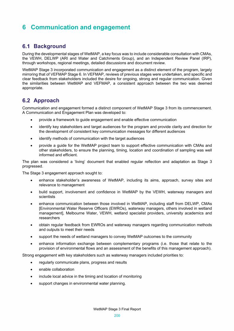
WetMAP Stage 3 Final Report
200
6 Communication and engagement
Background During the developmental stages of WetMAP, a key focus was to include considerable consultation with CMAs, the VEWH, DELWP (ARI and Water and Catchments Group), and an Independent Review Panel (IRP), through workshops, regional meetings, detailed discussions and document review.
WetMAP Stage 3 incorporated communication and engagement as a distinct element of the program, largely mirroring that of VEFMAP Stage 6. In VEFMAP, reviews of previous stages were undertaken, and specific and clear feedback from stakeholders included the desire for ongoing, strong and regular communication. Given the similarities between WetMAP and VEFMAP, a consistent approach between the two was deemed appropriate.
Approach Communication and engagement formed a distinct component of WetMAP Stage 3 from its commencement. A Communication and Engagement Plan was developed to:
provide a framework to guide engagement and enable effective communication
identify key stakeholders and target audiences for the program and provide clarity and direction for the development of consistent key communication messages for different audiences
identify methods of communication with the target audiences
provide a guide for the WetMAP project team to support effective communication with CMAs and other stakeholders, to ensure the planning, timing, location and coordination of sampling was well informed and efficient.
The plan was considered a ‘living’ document that enabled regular reflection and adaptation as Stage 3 progressed.
The Stage 3 engagement approach sought to:
enhance stakeholder’s awareness of WetMAP, including its aims, approach, survey sites and relevance to management
build support, involvement and confidence in WetMAP by the VEWH, waterway managers and scientists
enhance communication between those involved in WetMAP, including staff from DELWP, CMAs [Environmental Water Reserve Officers (EWROs), waterway managers, others involved in wetland management], Melbourne Water, VEWH, wetland specialist providers, university academics and researchers
obtain regular feedback from EWROs and waterway managers regarding communication methods and outputs to meet their needs
support the needs of wetland managers to convey WetMAP outcomes to the community
enhance information exchange between complementary programs (i.e. those that relate to the provision of environmental flows and an assessment of the benefits of this management approach).
Strong engagement with key stakeholders such as waterway managers included priorities to:
regularly communicate plans, progress and results
enable collaboration
include local advice in the timing and location of monitoring
support changes in environmental water planning.
WetMAP Stage 3 Final Report
201
Key messages and target audiences In the early phases of Stage 3, key messages focused on:
working closely with key stakeholders to make sure their information needs were met
the aim to inform and support environmental water planning and implementation
WetMAP monitoring of wetland vegetation, birds, frogs and fish
clarity around method, scientific rigour, and decision-making processes
awareness of limitations of scientific methods and/or data interpretation and
possible links with complementary programs.
There was a need to ensure key stakeholders contributed to and had confidence in Stage 3 from the start. Building a solid understanding of the approach taken (including the rationale for the approach) minimised the risk of differing expectations about what the results of WetMAP could demonstrate over time.
As Stage 3 proceeded, the foci of messages included details of progress of the various approaches, results, the interpretation of results, and management implications. It was emphasised in the first years of Stage 3 that many survey results were preliminary and could provide useful insights, but that a more comprehensive picture would be obtained nearer the completion of the stage.
Five types of target audiences were identified for WetMAP communication and engagement (see Figure 6.1). The key messages, and the themes and formats of engagement activities and communication products were developed in alignment with the needs of each audience. Understanding the interests and perspectives of each audience enables engagement activities to be targeted appropriately.
Figure 6.1: Target audiences for WetMAP Stage 3.
.
Ministers + Senior DELWP managers
Victorian and Commonwealth
waterway managers
Scientists
Interest groups and general
public
Traditional Owners
Agriculture and irrigation industries Recreational users –hunters, anglers, etc. Conservation groups including bird watchers, Community groups, e.g. Waterwatch Landholders Schools Local government
DELWP Universities – Victoria, across Australia International science community Consultant scientists
CMAs – including Environmental Water Reserve Officers network Melbourne Water DELWP, VEWH Murray‐Darling Basin Authority Commonwealth Environmental Water Office
Indigenous communities
Minister for Water (funder) Minister for Energy, Environment and Climate Change Senior managers in DELWP, e.g. Secretary, Executive Directors, Directors

WetMAP Stage 3 Final Report
202
Activities and methods for engagement A suite of activities and tools to engage with these audiences was identified in the Communication and Engagement Plan and formed the basis for an action (Table 6.1). Two specific citizen science projects relating to frogs and birds in wetlands were also undertaken (see Sections 6.5 and 6.6).
A communication register was established at the start of Stage 3 to record activities on a monthly basis. The register was updated monthly by project team members to ensure it captured the efforts of the WetMAP Project Team in a comprehensive way.
The following summary provides examples of how the different activities and tools were implemented and used (and see Figure 6.1).
Direct contact via phone and email WetMAP team members regularly spoke to and emailed key stakeholders, in particular EWROs within CMAs, to liaise on the planning of proposed surveys, share observations and recent survey results, and provide advice to support or modify proposed environmental flow events. This represented a substantial element of WetMAP communication and engagement, which supported waterway managers and informed environmental watering decisions to maximise outcomes from environmental watering events.
In late 2018, a ‘field survey update’ was initiated and distributed via email to stakeholders, to share early results of each survey with stakeholders. Such stakeholders included EWROs, waterway managers, DELWP regional staff, Parks Victoria and Trust for Nature staff relevant for each site. Field survey updates were theme-specific, and included:
Frogs: 2018 (two updates); 2019 (four updates); 2020 (one update)
Vegetation: 2019 (10 updates); 2020 (10 updates)
Birds: 2018 (one update); 2019 (17 updates); 2020 (eight updates)
Fish: 2018 (one update); 2019 (12 updates); 2020 (three updates).
Updates on the overall progress of the Program were also distributed to key stakeholders via email every 3–6 months by the Program Manager. The distribution list for these updates included CMAs, VEWH, Melbourne Water, DELWP CWCT, the PSC, IRP, MDBA, CEWO and PV.
Face-to-face meetings and workshops Meetings and workshops were held throughout the course of the project between WetMAP team members and key stakeholders. These included:
wetland site visits to discuss monitoring methods, findings and proposed environmental watering events
formal meetings with CMAs, VEWH and regional environmental water advisory groups, to discuss and seek guidance on Seasonal Water Proposals
a stakeholder workshop (March 2019) to discuss program progress and seek feedback
project team workshops to discuss KEQs and monitoring methods for each theme
IRP meetings to discuss program progress and seek feedback and advice
Project Steering Committee meetings twice-yearly
VEWH and WetMAP Communications Lead meeting to discuss working together more closely (January 2020)
DELWP and CEWO meeting to discuss alignment of environmental water programs (February 2018)
regular interactions between the WetMAP project team and members of other state and commonwealth environmental water programs [e.g. Environmental Water Knowledge and Research Monitoring, Evaluation and Research (EWKR/MER), Melbourne Water monitoring, The Living Murray].
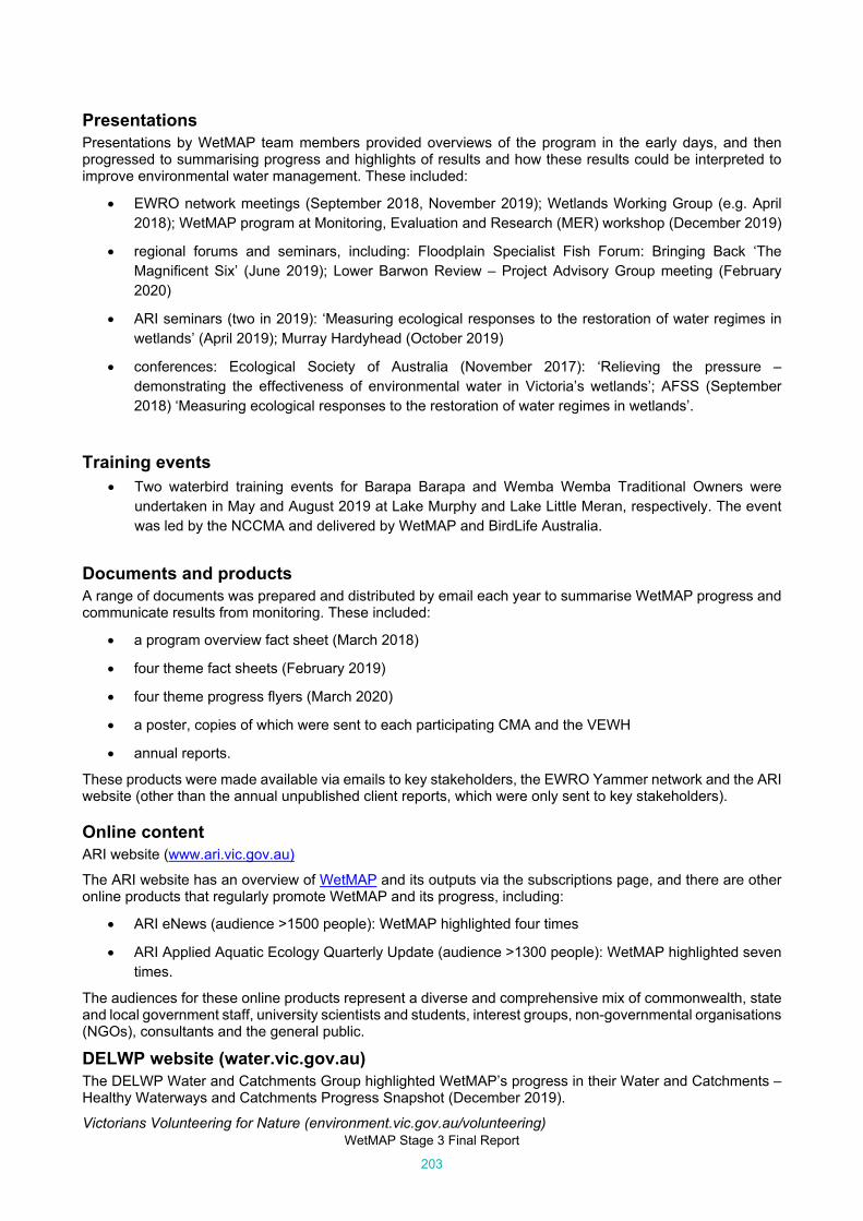
WetMAP Stage 3 Final Report
203
Presentations Presentations by WetMAP team members provided overviews of the program in the early days, and then progressed to summarising progress and highlights of results and how these results could be interpreted to improve environmental water management. These included:
EWRO network meetings (September 2018, November 2019); Wetlands Working Group (e.g. April 2018); WetMAP program at Monitoring, Evaluation and Research (MER) workshop (December 2019)
regional forums and seminars, including: Floodplain Specialist Fish Forum: Bringing Back ‘The Magnificent Six’ (June 2019); Lower Barwon Review – Project Advisory Group meeting (February 2020)
ARI seminars (two in 2019): ‘Measuring ecological responses to the restoration of water regimes in wetlands’ (April 2019); Murray Hardyhead (October 2019)
conferences: Ecological Society of Australia (November 2017): ‘Relieving the pressure – demonstrating the effectiveness of environmental water in Victoria’s wetlands’; AFSS (September 2018) ‘Measuring ecological responses to the restoration of water regimes in wetlands’.
Training events Two waterbird training events for Barapa Barapa and Wemba Wemba Traditional Owners were
undertaken in May and August 2019 at Lake Murphy and Lake Little Meran, respectively. The event was led by the NCCMA and delivered by WetMAP and BirdLife Australia.
Documents and products A range of documents was prepared and distributed by email each year to summarise WetMAP progress and communicate results from monitoring. These included:
a program overview fact sheet (March 2018)
four theme fact sheets (February 2019)
four theme progress flyers (March 2020)
a poster, copies of which were sent to each participating CMA and the VEWH
annual reports.
These products were made available via emails to key stakeholders, the EWRO Yammer network and the ARI website (other than the annual unpublished client reports, which were only sent to key stakeholders).
Online content ARI website (www.ari.vic.gov.au)
The ARI website has an overview of WetMAP and its outputs via the subscriptions page, and there are other online products that regularly promote WetMAP and its progress, including:
ARI eNews (audience >1500 people): WetMAP highlighted four times
ARI Applied Aquatic Ecology Quarterly Update (audience >1300 people): WetMAP highlighted seven times.
The audiences for these online products represent a diverse and comprehensive mix of commonwealth, state and local government staff, university scientists and students, interest groups, non-governmental organisations (NGOs), consultants and the general public.
DELWP website (water.vic.gov.au) The DELWP Water and Catchments Group highlighted WetMAP’s progress in their Water and Catchments – Healthy Waterways and Catchments Progress Snapshot (December 2019).
Victorians Volunteering for Nature (environment.vic.gov.au/volunteering)

WetMAP Stage 3 Final Report
204
This site included a frog citizen science project highlight for National Volunteer Week (May 2020). The frog project is also highlighted as an example of how Protecting Victoria’s Environment – Biodiversity 2037 is being implemented.
Other online content Other organisations that have produced online content related to WetMAP include:
VEWH o Annual ‘Reflections’ report (2017–2018, 2018–2019)
o ‘News and Stories’ on the VEWH webpage included the following WetMAP highlights:
– Gaynor Swamp – Exciting results from environmental watering in the Goulburn Wetlands (April 2019) (https://www.vewh.vic.gov.au/news-and-publications/stories/gaynor-swamp-exciting-results-for-environmental-watering-in-the-goulburn-wetlands)
– WetMAP frog citizen science project Jumping to get outdoors (November 2019) (https://vewh.vic.gov.au/news-and-publications/stories/jumping-to-get-outdoors-take-a-leap-and-become-a-frog-citizen-scientist)
– VEFMAP and WetMAP – the power of adaptive management of rivers and wetlands (December 2019) (https://www.vewh.vic.gov.au/news-and-publications/stories/vefmap-and-wetmap-the-power-of-adaptive-management-of-rivers-and-wetlands)
– WetMAP citizen science project: Birdwatching in northern Victoria (March 2020) (https://www.vewh.vic.gov.au/news-and-publications/stories/wetmap-citizen-science-project-birdwatching-in-northern-victoria)
CMAs – each CMA varies in its online content regarding environmental water; these have captured findings and work undertaken by WetMAP, mainly via media releases, field days, annual actions and achievement reporting.
o NCCMA – A hardy plan for an endangered fish (October 2017)
o MCMA – has developed Case Study flyers and media releases for WetMAP fish monitoring in Ducksfoot Lagoon and WetMAP bird monitoring at Heywoods Lake (still to be released)
BirdLife Australia website provided a primary avenue for the WetMAP Bird Citizen Science project (https://birdlife.org.au/)
The Frogs Are Calling You website (Frogscalling) provided the primary site for the WetMAP frog citizen science project (https://www.frogscalling.org/).
Online sites and newsletters occasionally shared and promoted WetMAP content (e.g. Finterest, Sydney University Society of Wetland Scientists Oceania Chapter).
Videos Videos provide a simple tool to engage audiences and promote WetMAP and its achievements.
A video is currently in development regarding the WetMAP Bird Citizen Science Project (this has been delayed due to COVID-19).
The NCCMA has produced a video to highlight the waterbird training activities with Traditional Owners (this has yet to be released).
The MCMA has developed a ‘Frogs of the Mallee’ video that mentions WetMAP (still to be released).
ARI recently released a video ‘Walking with scientists – a fieldwork showcase’, which includes WetMAP content (https://www.ari.vic.gov.au/research/field-techniques-and-monitoring/walking-with-scientists-vr-360).
Social media and networking Social media is a major way for many people to access and share information. DELWP has Facebook and Instagram pages (statewide and regional), and accounts with LinkedIn and Twitter. Examples of WetMAP content include:

WetMAP Stage 3 Final Report
205
Facebook: Rare salt bush recorded at Hird Swamp (March 2017); Murray Hardyhead (July 2019) Can you hear the frogs calling you? (October 2019)
Twitter: World Wetlands Day (February 2019).
Note, however, that there are some constraints on the type of content that can be delivered publicly on DELWP social media channels.
CMAs and Melbourne Water occasionally posted on social media; for example, there were Facebook posts and tweets regarding WetMAP progress and highlights, for example Butler Creek fish surveys (November 2018) by MCMA. These have proved a valuable avenue for sharing WetMAP activities with local audiences.
The EWRO Yammer network is an effective avenue for sharing WetMAP information with environmental water managers, and a substantial effort was made to post regularly on this site. Nine posts were produced: one in 2018, four in 2019 and four in 2020. Others in this network also posted about WetMAP content, for example MCMA regarding the release of Murray Hardyhead in Lake Hawthorn (November 2018).
DELWP internal networking DELWP has several avenues to promote WetMAP with internal staff, including Yammer groups and an intranet (Ada). Together, these have a combined potential audience of more than 4500. Posts on these forums have included:
five WetMAP-related posts on DELWP Yammer: three in 2020; two in 2019
two articles on Ada: World Wetlands Day (February 2019); Traditional Owner waterbird training event with NCCMA (May 2019).
WetMAP highlights have also been profiled in DELWP internal newsletters: ‘The Spill’ (Water and Catchments group) and ‘Yarn’ (Biodiversity group).
Media releases DELWP media releases provide a great opportunity to share news and are an effective way for stories to be picked up by local newspapers, radio and television. DELWP WetMAP media releases have included:
Murray Hardyhead hardy indeed (July 2018) (https://www.water.vic.gov.au/media-releases/2018/murray-hardyhead)
Science Week: Celebrating Citizen Scientists (August 2019) – frog project (https://www.wildlife.vic.gov.au/media-releases/science-week-2019-celebrating-citizen-science)
Waterbird monitoring with Traditional Owners (September 2019) (https://www.water.vic.gov.au/media-releases/2019/wetland-waterbird-monitoring-with-traditional-owners).

WetMAP Stage 3 Final Report
206
Table 6.1: Activities and target audiences.
Activities Victorian + Commonwealth waterway managers
Ministers Senior DELWP managers
Scientists Traditional owners
Interest groups and general public
Direct contact Phone calls Emails and Program updates Field survey update emails Face to face Meetings Workshops Presentations Regional forums and events ARI seminars External seminars (e.g. RBMS) Conferences Documents and products ARI Tech Reports, client reports Annual progress reports Fact sheets Posters and stickers Online content (websites, newsletters, etc.) DELWP and ARI website Other websites – VEWH, CMAs, CEWH, VFA, Rec fishing, Finterest)
ARI eNews ARI Applied Aquatic Ecology Quarterly Updates
ARI Applied Aquatic Ecology Quarterly Update (Influence)
Newsletter articles (VEWH, Finterest, RBMS, Basin News, Newstreams, ASFB)
Journal articles DELWP and ARI Videos Blogs, podcasts Social media and networking EWRO Yammer DELWP Facebook DELWP Twitter DELWP LinkedIn DELWP Instagram DELWP internal online networking Internal – DELWP Yammer Internal – DELWP Ada Internal – DELWP ‘The Spill’, and ‘Biodiversity Yarn’
Other media Media releases Newspaper articles Radio Television
ARI = Arthur Rylah Institute of Medical Research; DELWP = Department of Environment, Land, Water and Planning; VEWH = Victorian Environmental Water Holder; CMAs = Catchment Management Authorities; CEWH = Commonwealth Environment Water Holder; VFA = Victorian Fisheries Authority; Rec fishing = Recreational Fishing; RBMS = River Basin Management Society; ASFB = Australian Society for Fish Biology; EWRO = Environmental Water Reserve Officer

WetMAP Stage 3 Final Report
207
Figure 6.2: Examples of WetMAP Stage 3 communication and engagement activities and tools.

WetMAP Stage 3 Final Report
208
Evaluation of communication and engagement Stage 3 communication and engagement was adaptive, allowing for modification of approaches as it progressed. Given that aspects of Stage 3 (including survey design) changed over time, the primary focus was on ensuring key stakeholders were aware of and understood these changes. Further, more extensive, evaluation will occur preceding Stage 4 implementation, and when the program has progressed further (during Stage 4). Some general evaluation has, however, been undertaken regarding:
the communication and engagement outputs, in terms of undertaking identified activities and use of tools for target audiences, achievement of milestones and targets (e.g. number of flyers or publications produced, number of meetings, workshops attended)
the communication and engagement outcomes, their extent and quality (e.g. changes in awareness of WetMAP, how attitudes towards the project have changed).
Communication and engagement outputs Regular updating and sharing of the communication and engagement activities register enabled the project team to keep track of conversations with and actions and responses of stakeholders to communication and engagement. Regular project team meetings and frequent strong communication across the team enabled milestones to be met, and the opportunity for reflection on activities and tools with which to engage with target audiences.
Many insights have been gained regarding the effectiveness of activities and tools used for Stage 3 communication and engagement; these will prove valuable during the planning and implementation of Stage 4.
Activities and tools for engagement
Direct contact via phone and email
Regular direct interactions, via phone calls and email updates between WetMAP team members and the key stakeholders within CMAs were effective in building connections and providing advice to support or modify proposed environmental flow events.
The Field Survey Updates provided a particularly valuable method of advising key stakeholders of survey findings in a timely way. They enabled highlights and interesting findings to be easily shared, as well as including a selection of photographs to illustrate key messages. This initiative was well received by many stakeholders and based on this positive response we commenced similar field survey updates in VEFMAP. Stakeholders have indicated that they are very helpful in supporting upcoming seasonal watering planning.
Face-to-face meetings and workshop
Successful collaboration with wetland managers was facilitated via site visits and more formal meetings with CMAs and the VEWH to discuss environmental flow planning. The opportunity to incorporate more structured input of WetMAP staff to the development of Seasonal Watering Proposals should be further investigated.
Stakeholder workshops, IRP meetings and PSC meetings provided useful opportunities for evaluating and reviewing Stage 3 progress, including communication and engagement. The involvement of WetMAP staff in other environmental water programs (e.g. VEFMAP) and participation in workshops and meetings with the CEWO’s Flow-MER team contributed to increased alignment between related programs.
Participation of key stakeholders in field trips provided a useful method of building relationships and should be encouraged further.
Relationships between the WetMAP Communications Lead and CMAs, VEWH and DELWP communication staff have been enhanced.
There has been strong connection with bird and frog enthusiasts via the WetMAP citizen science projects (for more detail see Section 6.5 and 6.6).
Positive feedback from NCCMA and Barapa Barapa and Wemba Wemba Traditional Owners was obtained from two waterbird training events held at Lake Murphy and Little Lake Meran, where WetMAP scientists, BirdLife Australia volunteers and Traditional Owners from the Barapa Barapa met at Lake Murphy. Aboriginal Water Officers have expressed interest in participating in future field trips, which would provide a valuable means of engagement and will be pursued in the next stage of WetMAP.

WetMAP Stage 3 Final Report
209
Presentations
Attending and presenting at EWRO meetings was a useful way of sharing WetMAP progress. Presentations were given at regional forums and events, and WetMAP team members will continue to liaise with CMAs to identify high priority events to focus on in order to reach a diverse range of local audiences.
ARI seminars provided a valuable opportunity to promote progress, albeit to a relatively small, targeted audience of predominantly DELWP staff.
Participation in conferences provided an important opportunity to highlight the WetMAP approach and its findings to scientists from Australia and internationally. Efforts to attend and present at conferences will likely increase in the next few years as journal articles and reports are released. Consideration should be given to which regional, state and commonwealth forums could allow engagement with other important target audiences not yet the focus of WetMAP communications.
Documents and products
Annual unpublished client reports and fact sheets have been well received by key stakeholders. Now the results of Stage 3 have been finalised, there will be further opportunities to prepare distinct stories and communication outputs.
Online content
Ensuring up-to-date WetMAP content is available on ARI and DELWP websites is a fundamental requirement and will continue. Inclusion of WetMAP content within ARI eNews and Applied Aquatic Ecology Quarterly Updates will likely increase as Stage 3 outcomes are finalised. These avenues are particularly valuable for sharing information across a broad range of target audiences.
Efforts to build and maintain strong relationships with VEWH and CMA staff have been valuable, facilitating sharing of stories regarding WetMAP findings. It would be worthwhile increasing efforts to provide content for other online sites and newsletters, including broadening connections with other target audiences (e.g. conservation groups, interest groups (hunting groups), the irrigation industry and Indigenous audiences).
Videos provide a simple tool for engaging audiences, and it would be valuable to prepare a DELWP video to summarise the Stage 3 achievements, as well as highlight the methods used for monitoring the four themes. There may also be opportunities to work with CMAs and other collaborators on external videos.
Social media and networking
Regular posting on the EWRO Yammer network and DELWP social media has proved valuable for sharing WetMAP information and ensuring results are communicated to a wider audience via social media platforms. EWRO Yammer posts often initiated conversations within the network between stakeholders, including sharing further details, interpretation and highlights.
Internal DELWP online networking
Regular posting on DELWP’s Yammer network effectively promoted WetMAP to a broad DELWP audience, including senior managers and communication staff. This proved useful for garnering interest for further promotion and should continue. Similarly, development of WetMAP content for Ada and the fortnightly internal newsletters (e.g. The Spill) should continue.
Engagement outcomes Evaluation of engagement outcomes has focused on the attitude towards and awareness of WetMAP among wetland and waterway managers, primarily via direct feedback and liaison, and also through less formal feedback such as the EWRO Yammer and direct contacts. Overall, this feedback has been encouraging and indicates there is a clear awareness of this program.
Feedback has been sought directly during stakeholder meetings and email communication to stakeholders from the Program Manager and the Communication Lead – and has also been provided to the ARI Coordinator following receipt of the Field Survey Updates. Most feedback has been informal and general in nature, with no specific concerns expressed by stakeholders. The Field Survey Updates have been very well received, and stakeholders have indicated that they are very helpful in supporting upcoming seasonal watering planning.

WetMAP Stage 3 Final Report
210
Highlights
Project Team communication
The WetMAP project team included a large number of staff from the DELWP Water and Catchments Group and ARI, BirdLife Australia, Frogs Victoria, and a range of consultants with varying levels of involvement. Through a clear governance and reporting structure, a strong team ethos was established at the start and continued throughout Stage 3. Monthly meetings were held to discuss progress, issues and actions, and by following a regular, clear process, this ensured all members of the project team were kept up to date, lines of communication were open and effective, and comprehensive records were maintained. The preparation of Quarterly Progress Reports also contributed to maintaining open lines of communication across the team.
Working with waterway managers and EWROs
Over time, the strength of the relationships and understanding between the WetMAP project team and waterway managers, EWROs, and relevant communication staff have increased. There has been regular liaison during planning and implementation of field surveys, discussion of results and provision of advice on environmental watering.
The WetMAP Communication Lead and ARI’s Science Manager, Communication and Collaboration, are now members of the Victorian CMA’s Communications Forum, which meets every two months, helping to build more effective connections with our CMA partners. Similar connections with DELWP Water and Catchments, Biodiversity, and Corporate Communications staff continue, which contributes to sharing WetMAP progress and achievements across the Department.
Recommendations for Stage 4 As WetMAP Stage 4 planning commences, it will be timely to continue to build on existing connections with key stakeholders as well as expand efforts to communicate and engage with a broader range of target audiences.
Stage 4 Communication and Engagement Plan Preparation of a Stage 4 Communication and Engagement Plan will include reflection on the content of the Stage 3 plan. Specific actions to be considered for inclusion within Stage 4 include:
continuing to strengthen connections with VEWH and CMA communication and waterway management staff to support promotion of WetMAP and its findings
investigating opportunities to build stronger connections with Aboriginal Water Officers, irrigation and agricultural industry contacts, and interest groups associated with wetlands (e.g. Field and Game)
investigating other summary outputs that are more suitable to the general public, including increased use of infographics and visually appealing approaches. This could include fact sheets with brief summaries and simple messages of interest that are relevant and understandable to local communities (e.g. comparisons of the number of fish over years), with clear, simple graphs and photographs
producing videos to highlight WetMAP’s aims, activities, findings and achievements
continuing to explore opportunities to promote WetMAP achievements via DELWP online and social media, while placing a focus on producing content for regional DELWP social media
investigating opportunities to increase connections with a broader range of interest groups to ensure they are aware of WetMAP and its progress and encourage sharing of WetMAP content on external e-newsletters and blogs
working with CMA staff and other relevant organisations to identify appropriate regional forums and events through which to share information about WetMAP progress.

WetMAP Stage 3 Final Report
211
Citizen science
The benefits of citizen science in ecological research and monitoring Scientific data collection by the general public, known as citizen science, is becoming increasingly popular as a method to increase data collection and as an outreach and engagement tool. There is government and public interest in citizen scientist participation in environmental monitoring programs, and there is increasing confidence in the scientific accuracy and validity of large datasets generated by the public (Roy et al. 2012), particularly when the potential for error is considered in project design (Brown et al. 2018). In a well-designed citizen science project, data collected by the public are indistinguishable from data collected by professional research scientists (McKinley et al. 2016). Citizen science projects can successfully advance scientific understanding, inform policy issues and supplement existing government monitoring programs (Bonney et al. 2009). There are also clear cost savings when volunteers participate in monitoring programs (Bodilis et al. 2014). Additional benefits of public engagement in science include improving scientific literacy and interest, increasing participants’ awareness of specific issues, and fostering local stewardship (Gillett et al. 2012; Miller-Rushing et al. 2012). Citizen science projects can enable greater interactions between scientists and the public, which can in turn lead to an improved understanding of each other’s perspectives and interests (Bela et al. 2016). Participants in citizen science may obtain new skills and knowledge, and there is also the potential to promote changes in behaviour (McKinley et al. 2016).
To investigate broad-scale ecological patterns, researchers are required to collect a significant amount of data at multiple scales. One way to achieve this requirement is through citizen science, which partners communities with professional researchers, and embeds them in the data collection process (Bonney et al. 2009; Newson et al. 2015). These partnerships build capacity within communities and encourage knowledge exchange between institutions and the public. Targeted citizen science projects can also appeal to local skillsets to engage participants and establish regional data collection networks. Additional aims (and benefits) of citizen science projects are often to cultivate learning, connection to nature and the environment, and to inspire communities to be proactive about conservation.
Data generated through citizen science, once analysed, can reveal patterns in species behaviour and distribution, as well as wider population trends. Even weakly structured citizen science surveys can generate robust data that can reveal significant ecological knowledge (Szabo et al. 2012). Szabo et al. (2012), for example, demonstrated that volunteer-collected and unstructured atlas data can be used to generate occupancy models and population estimates for many Australian bird species at a regional scale. Increasingly, results from citizen science projects inform natural resource management and feature in peer-reviewed scientific research seeking to answer a broad range of ecological questions (Hurlbert and Liang 2012; Jackson et al. 2016; Studds et al. 2017). Studds et al. 2017, for example, demonstrated widespread declines in migratory shorebirds in Australia, with rate of decline correlating with the extent to which their migration stopovers overlap with threatened tidal flats in the Yellow Sea. Citizen science data has made a clear and credible contribution to the field of ecology, particularly ornithology (Cooper et al. 2014), and this is expected to continue.
In most citizen science projects, the public is asked by scientists to collect and contribute data or samples, most often in an incidental or ad hoc fashion (Roy et al. 2012). This approach enables scientists to have a significant level of control to ensure greater data accuracy, while still engaging the public (Sbrocchi 2014). Contributory projects can facilitate the participation of large numbers of volunteers yet can also be relatively straightforward to manage.
Citizen science projects can increase ‘social capital’, which is measured by increases in trust, harmony and cooperation within communities involved in monitoring programs. Where programs provide rewards, such as personal satisfaction and enjoyment through socialisation, there is likely to be longer retention of volunteers, which in turn reduces the effort required for training and administration (Sbrocchi 2014). Projects need to maintain a strong emphasis on ongoing training and monitoring.
Citizen science in Victorian Government In Victorian Government, citizen science is acknowledged within two key Victorian plans: ‘Water for Victoria’ (DELWP 2016) and ‘Protecting Victoria’s Environment – Biodiversity 2037’ (DELWP 2017).
‘Water for Victoria’ (DELWP 2016) identifies the role of citizen science within two key Victorian plans:
o Action 3.4 – Provide long-term investment to improve waterway health
o Action 3.8 – Support community partnerships and citizen science.

WetMAP Stage 3 Final Report
212
‘Protecting Victoria’s Environment – Biodiversity 2037’ Strategy (DELWP 2017) via two goals: (i) Victorians value nature and (ii) Victoria’s natural environment is healthy. The project was relevant to following priorities:
o increase the collection of targeted data for evidence-based decision-making
o raise the awareness of all Victorians about the importance of the state’s natural environment
o increase opportunities for all Victorians to have daily connections with nature
o increase opportunities for all Victorians to act to protect biodiversity
o support and enable community groups, Traditional Owners, NGOs and Chapters of government to participate in biodiversity response planning.
Pilot projects WetMAP implemented two pilot citizen science projects, one that focused on frogs (‘The Frogs Are Calling You’) and the other focused on birds.
Background
Frog citizen science
Frog research studies are particularly good candidates for the incorporation of citizen scientists. Frogs are charismatic, accessible and widespread, and there are many examples of projects with citizen science components (Weir and Mossman 2005). Interested citizens have regularly contributed information on frog occurrence to the Atlas of Living Australia and, more recently, the Australian Museum FrogID Project. In Victoria, frog records are regularly submitted by the public to the DELWP Victorian Biodiversity Atlas and programs run by the Goulburn Broken, North Central and Mallee Catchment CMAs. The Melbourne Water Frog Census (the successor to Frog Watch) encourages public participation in frog surveys in and around Melbourne.
Bird citizen science
In Australia, there is a range of citizen science projects aimed at monitoring birds. These projects operate across a diverse array of ecosystems and at various scales. Each is designed to answer scientific questions while engaging with the public via bird ecology. BirdLife Australia facilitates many citizen science projects and manages the largest national database of bird records via Birdata. A common theme of the projects delivered by BirdLife Australia is that they enable citizens to contribute to scientific projects with specific aims of demonstrating ecological relationships. The Shorebirds 2020 project (now known as the Australian National Shorebird Monitoring Project) is one such project that aims to characterise shorebird population trends in both the long and short terms, and that explores drivers for these changes. This project generates a significant amount of data pertaining to shorebird congregations in wetlands across Australia. Regionally, the Powerful Owl Project enlists citizen scientists across south-eastern Australia to monitor the distribution and abundance of this species and has uncovered that approximately 31% of suitable habitat for this species was impacted by the most recent bushfires. Similarly, the Great Pelican Count is designed as an annual snapshot census of Pelican numbers across the Gippsland Lakes. It is held on the same day and at the same time, across 91 locations, and is a substantial community-led effort structured around the conservation of an iconic species. At the system-level, the Lake Cullen Citizen Science Project boosted the number of surveys across the Kerang Lakes and generated data for a generally under-surveyed area. This project produced new insights into the dynamic use of the wetland throughout an environmental watering cycle and helped provide information about threatened species populations including the Australasian Bittern (Botaurus poiciloptilus).
Project aims Both citizen science pilot projects shared the following aims:
to provide a meaningful and satisfying citizen science program for both scientists and volunteer participants
to build the scientific capacity of citizens in monitoring frogs and/or birds
to enhance broader community awareness of WetMAP and its monitoring approach

WetMAP Stage 3 Final Report
213
to enhance broader community awareness and understanding of the benefits of environmental water, how it is managed, and the information used to inform environmental flow decisions
to grow Victorians’ connections with nature and actions for nature
to increase our understanding of the motivations, sense of meaning of activity, and role of Special Places for participants
to obtain supplementary observations to those obtained through the standardised monitoring program, to increase the dataset and provide a fuller understanding of frog and/or bird occurrence.
For both citizen science projects, evaluation of citizen science data compared with WetMAP monitoring data was considered. Both projects were designed to ensure and verify the quality of citizen science data. However, this additional aspect was not progressed because the amount of data that was gathered was not sufficient to support these comparisons. This will be progressed in the next stage of WetMAP.
Approach Frogs Led by Lynette Plenderleith of Frogs Victoria, the project established a strong collaboration with the University of Melbourne, the Australian Museum, the NCCMA and Goulburn Broken CMA (GBCMA). The project was branded ‘The Frogs Are Calling You’ to increase engagement and exposure with the public and to reflect on the collaborative nature of the project beyond ownership by WetMAP. Additionally, the branding optimised online searching and provided specific social media products such as #frogscalling.
Birds Led by BirdLife Australia, this project focused on the GBCMA region, with a view to expand to more CMAs regions with current WetMAP sites in future years. This project established a strong collaboration between DELWP, BirdLife Australia, BirdLife Murray–Goulburn and the GBCMA.
Communication and Engagement Plans were developed for both projects to provide:
clarity and direction for the development of consistent key messages arising from both projects
recommended methods to guide engagement approaches and enable effective communication
guidance for the citizen science project teams on communicating effectively with citizen scientists and other stakeholders to ensure the planning, timing, location and coordination of sampling was well informed and efficient.
These plans were ‘living’ documents, which enabled regular reflection and adaptation. They adopted the International Association of Public Participation spectrum (IAP2), which recognises that differing levels of engagement are legitimate depending on the context. The spectrum ranges from the simple one-way information flow of ‘Inform’, through increasing levels of stakeholder participation in ‘Consult’ and ‘Involve’, to genuine partnerships in ‘Collaborate’ and ‘Empower’.
Communication and engagement with current and potential citizen participants were at the core of the projects, being tied to the achievement of the project objectives. Participation with these citizen scientists can range across the IAP2 spectrum. The approach to communication and engagement for the variety of other target audiences is different and for some may be restricted to Inform. This is particularly true in the early stages of these pilot projects.
Target audiences
Target audiences for these projects aligned with those identified within Figure 6.1: Victorian waterway managers; ministers and senior DELWP managers; Commonwealth waterway managers; scientists; interest groups, citizen science groups, private landholders and the general public. The interest groups incorporated citizen science groups such as the Australian Citizen Science Association and the Australian Museum, who manage the FrogID project and app.
Key messages Communication in these projects was framed around the following key messages:
1. Citizen science is for anyone, regardless of education, training and scientific literacy. It’s fun, easy and is an opportunity to enjoy science as well as learn something.
2. Frogs and birds are integral to the health of the environment and it’s vital we know how environmental water affects their ecology.

WetMAP Stage 3 Final Report
214
3. Water is a scarce resource and it’s vital that we use it efficiently.
4. Citizen science data can help build on our understanding of the presence and diversity of frogs and birds in and around WetMAP focal wetlands and the wider landscape.
5. It is possible to engage in the project at different levels of participation depending on commitment and enthusiasm.
Messages sought to align with water for the environment communication from the state and commonwealth government agencies (i.e. DELWP, VEWH, CEWH, MDBA).
WetMAP frog citizen science Engagement methods, outputs and project highlights This is a pilot project, and progress was constrained by COVID19 restrictions. A suite of activities and tools to engage with target audiences were identified and formed the basis for an action plan for their implementation. This included direct contact (including via email and phone calls), presentations, preparation of documents (a flyer and poster) and online and social media content. A brief summary of highlights is provided below (see Appendix 20 for further details).
Direct contact and presentations
The WetMAP frog citizen science project lead initiated and maintained contact with key collaborators to foster support and broaden reach of the project. This included NCCMA, GBCMA, Mallee CMA, Waterwatch and other DELWP contacts. Several meetings were held to discuss options for promoting the project and reaching potential participants. Correspondence continues between the project lead and collaborators to maximise potential for collaboration and project impact.
A presentation on the frog citizen science project was given at the WetMAP bird citizen science field day in Shepparton (February 2020). The event was attended by BirdLife members and interested local parties, many of whom expressed an interest in frogs and the frog citizen science program. A few reported that they already use the FrogID app while birdwatching and/or otherwise outside.
Online content
Information on the project was provided on the DELWP and ARI websites. In order to reach a broad and remote audience, emphasis was placed on creation of a specific project website and regular social media efforts. A specific project website was considered the most effective tool for instructing participants, promoting the project, garnering interest and sharing progress. The frogscalling.org website was created as the primary conduit for project information and progress and launched in August 2019 (Figure 6.3). This website comprises:
About – project overview, links to collaborators, environmental water management information social media links, etc.
News – Croak newsletter (released quarterly. Includes editor’s letter, data analysis/report, featured frog, broad science article, citizen spotlight, field report, lab report, WetMAP science article), and links to media content
Events – field days (these have not yet proceeded)
Sign Up – steps to sign up, and link to questionnaire
Instructions for data collection – steps to load FrogID app, how to become a champion, health and safety information, habitat data collection sheet, map of WetMAP survey sites
FAQs – further clarification for data collection and project mechanisms
Contact us – a contact form and links to social media.
Social media
The Frogs Are Calling You uses social media platforms to recruit citizen scientists, as well as inspire, engage and educate its audience about the project, environmental water, frogs, biodiversity and WetMAP (Table 6.2). The social media presence supplements communications through the website, newsletters and email list. It aims to provide the sense of community that is not otherwise established by field work performed as an individual in remote areas.

WetMAP Stage 3 Final Report
215
The target audiences are potential citizen scientists, people that haven’t heard of WetMAP and people who would like to learn more about frogs and environmental watering.
In addition to the specific social media goals outlined above, a measure of success of the wider communication and engagement aims will be included in the wider-reaching analysis, such as the engagement questionnaire.
Platforms include:
Facebook (/frogscalling) 120 followers (as of 17 July 2020). This is good for longer-form posts; great for imparting information; generally suits an older audience; and links to other platforms
Instagram (@frogscalling) 312 followers, 53 posts (as of 17 July 2020). This engages primarily through photographs/visual posts; capitalises on the charisma of frogs and natural beauty of sites; and is great for recruitment and short-form information
Twitter (@frogscalling) 90 followers, 46 tweets as of 17 July 2020. This promotes networking with similar organisations and is used to provide links to longer-form content.
Figure 6.3: The Frogs Are Calling You website landing page. Table 6.2: Social media aims and analysis measures for The Frogs Are Calling You.
Objective Social media goal Metric Recruit citizen scientists Raise project profile Number of citizen scientists that discovered the project
through social media Expand audience Reach people outside of
the project Number of followers and shares
Environmental advocacy Posts about frogs, habitat and environmental water
Number of questionnaire respondents that report behavioural change
Encourage a sense of community
Posts by or from citizen scientists and/or wider community
Engagement statistics, number of user-generated or -submitted posts
Content posted:
1. Data collection instructions To augment the website, particularly as many citizen scientists don’t read or comprehend it all in webpage form. To further clarify instructions for those unsure and reluctant to ask for assistance. May also inspire more participants to sign up or collect more data.

WetMAP Stage 3 Final Report
216
2. Friday FAQS To augment the website – we receive many questions that duplicate the questions on the FAQs page. Can include some reformatted instructions.
3. Incitement Posts that aim to inspire recruitment or further data collection. For example: ‘Perfect weather to collect some frog call data this weekend.’
4. Further information More in-depth educational resources about frogs, environmental watering, WetMAP and science.
5. Current affairs/pop culture Seasonal content to show we are up to date and informed about observance days, etc. Examples include World Water Day, World Frog Day.
Posting schedule:
As social media are used more, insights into the optimal posting times can be gleaned to inform scheduling. At time of writing, Saturday lunchtime is optimal for Facebook.
New content should be posted two to three times a week to maintain ranking by social media platforms, but posting is limited by content, particularly the number of available photographs. Content is currently posted on The Frogs Are Calling You social media accounts at least once a week.
WetMAP bird citizen science
Engagement methods, outputs and project highlights This is a pilot project, and progress was constrained by COVID19 restrictions. Multiple methods of engagement with target audiences were implemented. These ranged from direct contact, face to face meetings, presentations, training workshop, flyers, a bird identification guide, as well as social and online media content, and project updates via email. A summary of highlights is provided below (see Appendix 21 for further details).
BirdLife Australia aimed to engage with and recruit potential citizen scientists through four main channels:
directly via BirdLife Australia’s central social media and mailing lists activating networks maintained by BirdLife Australia’s Murray–Goulburn Branch indirectly via outreach to community groups that align with the projected values and objectives of
WetMAP and
a community training workshop. An email to BirdLife members from the Greater Shepparton region was sent to engage potential participants; it reached approximately 720 members and encouraged them to register as citizen scientists for the project.
Identification Guide
The ‘Waterbirds of South Eastern Australia’ identification guide was a notable output from this project.
Direct contact
BirdLife Australia’s Murray–Goulburn Branch is dynamic and effective. The WetMAP Bird Citizen Science Project lead sought direct feedback from these members and integrated their rich wealth of experience into the development of the focused workshop (details below). This approach invited direct involvement from an element of the target audience, which built local enthusiasm for upcoming actions. Post-workshop, BirdLife Australia Murray–Goulburn coordinated their survey efforts around watering events. The group has provided further feedback on the direction of program and is eager to participate in the future.
The WetMAP Bird Citizen Science Project lead maintained regular contact with key stakeholders to discuss opportunities to promote the project and recruit citizen scientists, and other logistical matters.
Presentations – A Wetland Bird Ecology and Identification Workshop
Delivering a workshop on wetland bird ecology and identification provided a key opportunity to recruit and train participants. While many experienced bird enthusiasts can already contribute robust data, casual birdwatchers may have needed some initial training and guidance to confidently participate in the project. This workshop provided an avenue to achieve a baseline skill level, which ensured the collection of usable data. The workshop
WetMAP Stage 3 Final Report
217
included presentations about WetMAP, so it was also an opportunity for participants to connect and begin self-organising around bird monitoring in response to the delivery of environmental water.
The workshop was held in Shepparton in February 2020 and was attended by approximately 50 people (Figure 6.4). The workshop represented a strong collaboration with the GBCMA, BirdLife Australia Murray–Goulburn, River Connect (Greater Shepparton City Council), DELWP ARI and the WetMAP frog citizen science project lead. Presentations were given that outlined environmental water and its management; WetMAP and its progress; other citizen science projects; and bird identification and use of Birdata. There was then a site visit to Shepparton Wastewater Treatment Plant, where participants operated scopes, recorded waterbirds and applied their identification training in the field.
Figure 6.4: Training workshop in Shepparton. Birds seen at Shepparton Wastewater Treatment Plant [Pink-eared Ducks (Malacorhynchus membranaceus), Australasian Shovelers (Anas rhynchotis), Grey Teal (Anas gracilis) and Hardhead (Aythya australis)].
Data collected Since the start of 2020, citizen scientists completed 41 surveys across six WetMAP wetlands (Black, Doctors, Kinnairds, Moodie and Reedy swamps and Loch Gary). These surveys were conducted by seven individual citizen scientists and comprised both main water body area (33) and riparian block searches (8). Overall, citizen scientists detected 35 waterbird species and 62 woodland bird species during this time (Figure 6.5). Pacific Black Duck (Anas superciliosa) was the most frequently detected waterbird species across these wetlands, with a reporting rate of 0.54. Galah (Eolophus roseicapillus; reporting rate: 0.82) and Noisy Miner (Manorina melanocephala; reporting rate: 0.61) were among the most frequently detected woodland bird species by citizen scientists. Of the shorebirds, citizen scientists detected Masked Lapwing (Vanellus miles) the most (reporting rate: 0.42), while the White-faced Heron (Egretta novaehollandiae) was the most frequently detected large wading species (reporting rate: 0.32). Few piscivores were detected across the WetMAP wetlands during this time. The Australian Pelican (Pelecanus conspicillatus) was the most frequently detected of these, with a reporting rate of 0.12.

WetMAP Stage 3 Final Report
218
Figure 6.5: Species accumulation curves across all WetMAP wetlands using citizen science data collected since the start of 2020.
Preliminary evaluation As citizen science continues to evolve in Victoria, it is useful to build our understanding of the factors driving participant satisfaction in citizen science programs. Few studies rigorously assess the effectiveness of the connection between participation in citizen science projects and behavioural change. There are several measures that can be used to assess success, including participant satisfaction, the value of the scientific contributions and a change in scientific literacy or behaviour for participants (Bonney et al. 2009). Such measures have been incorporated into the evaluation approaches for both the frog and bird citizen science projects. Both pilot projects are still in their early stages, and so comprehensive evaluation of communication and engagement is premature. Both, however, have developed questionnaires to assist in the assessment of projects; these questionnaires take into consideration the specific objectives of the projects (see Appendices 7b and d). They have sought to incorporate an adaptive model, allowing for modification of approaches as they progress. The next stage of WetMAP’s citizen science projects will continue to include measurable objectives and gather data to assess project success, both during and after project implementation.
Recommendations for WetMAP Stage 4 citizen science Frogs
Continue participant recruitment through local and state-wide media. The number of school children that signed up to the program as part of a school project suggests that there is a great potential for citizen science recruitment through schools. This will be a focus of future recruitment, although it is unlikely that the involvement of children will increase data collection at WetMAP focus sites. Many citizen scientists cited their children as being motivators for participation, further suggesting that children are a good avenue for promotion.
Further encourage the audience questionnaire to provide more robust insight into behavioural change and education of participants.
Place a greater emphasis on encouraging data collection at WetMAP focal sites, including more mention of the sites on social media and in the newsletter.
Continue to produce the Croak newsletter and social media campaigns. The outreach component of the project has been successful and shows great promise for further fostering support for environmental water and biodiversity.
Consider expansion to incorporate more CMAs with current WetMAP sites (Mallee and Wimmera CMA regions) in future years.

WetMAP Stage 3 Final Report
219
Birds A range of recommendations worthy of consideration are listed below:
Undertake improved communication of wetland watering and professional survey schedules. While there are significant logistical considerations that determine when wetlands are watered and professionally surveyed, clarity in this area will allow for better coordination of citizen scientists and implementation of engagement strategies. This is particularly important for investigating concordance between citizen science data and professional data, which requires extensive planning.
Undertake regular community-led field trips. While the monitoring regime has so far been unstructured, supporting regular community-led field trips could prove beneficial in multiple ways. First, it could ensure wetlands and their riparian blocks are surveyed regularly (e.g. monthly). Regular community-led field trips could also be a powerful tool in bridging skill gaps in the community by connecting novices with skilled birders. They also pose an opportunity to further engage and communicate with citizen scientists.
Undertake community forums to accompany workshops. Citizen science is a partnership between professionals and the community. Information and knowledge flow in multiple directions. The project will benefit from more opportunities for open dialogue among the WetMAP team and citizen scientists. Ideally, community forums will replace workshops, as objectives shift away from training towards sharing and celebrating research.
Engage more with Traditional Owners. While Traditional Owners were identified as a part of our outreach strategy, there are opportunities to form genuine partnerships with these groups via the WetMAP Bird Citizen Science Project. Further engagement and collaboration with the Yorta Yorta Nation Water Officer could be considered a starting point but should be a part of a wider Traditional Owner participatory approach.
Consider other survey methods, including ecoacoustic monitoring. By entrusting local birders with ecoacoustic monitoring devices, the WetMAP Bird Citizen Science Project could facilitate stewardship of wetlands and ensure the flow of verifiable data through a data-sharing agreement with the community.
Investigate the development of an experimental/survey design to allow an explicit comparison of WetMAP monitoring with citizen scientist monitoring.
Develop a ‘Wetland Bird Hub’ similar to the ‘Beach Nesting Bird Hub’ (https://beachvol.birdlife.org.au/login/index.php), which provides a platform for regular feedback, training and the communication of results. This is important for maintaining motivation, stewardship and project validation.
To fully understand the role and value of wetlands that receive environmental water, we need to understand the interactions with other sites. In future, WetMAP citizen science could include more wetlands that do not have managed water regimes. Data from these wetlands would help in the understanding of processes occurring in watered wetlands, such as breeding. Objectives for a broader program would be informed by the key knowledge gaps identified in the WetMAP bird monitoring program (see Chapter 5).
References Bela, G., Peltola, T., Young, J.C., Balázs, B., Arpin, I., Pataki, G., Hauck, J., Kelemen, E., Kopperoinen, L.,
Van Herzele, A., Keune, H., Hecker, S., Suškevics, M., Roy, H.E., Itkonen, P., Kulvik, M., Lászlo, M., Basnou, C., Pino, J. and Bonn. A. (2016). Learning and the transformative potential of citizen science. Conservation Biology 30 (5), 990–999.
Bodilis, P. Louisy, P., Draman, M., Arceo, H.O. and Francour, P. (2014). Can citizen science survey non-indigenous fish species in the eastern Mediterranean Sea? Environmental Management 53, 172–180.
Bonney, R., Cooper, C.B., Dickinson, J., Kelling, S, Phillips, T, Rosenberg, K.V. and Shirk, J. (2009). Citizen science: a developing tool to expanding science knowledge and scientific literacy. BioScience 59 (11), 977–984.
Brown, G., McAlpine, C., Rhodes, J., Lunney, D., Goldingay, R., Fielding, K., Hetherington, S., Hopkins, M., Manning, C., Wood, M., Brace, A. and Vass, L. (2018). Assessing the validity of crowdsourced wildlife observations for conservation using public participatory mapping methods. Biological Conservation 227, 41–151.
WetMAP Stage 3 Final Report
220
Cooper, C.B., Shirk, J. and Zuckerberg, B. (2014). The invisible prevalence of citizen science in global research: migratory birds and climate change. PLOS One 9 (9), e106508.
Gillett, D.J., Pndella, D.J., Freiwald, J., Schiff, K.S., Caselle, J.E., Shuman, C. and Weisberg, S.B. (2012). Comparing volunteer and professionally collected monitoring data from the rocky subtidal reefs of Southern California, USA. Environmental Monitoring and Assessment 184, 3239–2357.
Hurlbert, A.H. and Liang, Z. (2012). Spatiotemporal variation in avian migration phenology: citizen science reveals effects of climate change. PLOS One 7 (2), e31662.
Jackson, M.C., Weyl, O.L.F, Altermatt, F., Durance, I., Friberg, N., Dumbrell, A.J., Piggott, J.J., Tiegs, S.D., Tockner, K., Krug, C.B., Leadley, P.W. and Woodward, G. (2016). Recommendations for the next generation of global freshwater biological monitoring tools. Advances in Ecological Research 55 doi:10.1016/bs.aecr.2016.08.008.
McKinley, D.C., Miller-Rushing, A.J., Ballard, H.L., Bonney, R., Brown, H., Cook-Patton, S.C., Evans, D.M., French, R.A., Parrish, J.K., Phillips, T.B., Ryan, S.F., Shanley, L.A., Shirk, J.L., Stepenuck, K.F., Weltzin, J.F., Wiggins, A., Boyle, O.D., Briggs, R.D. and Soukup, M.R. (2016). Citizen science can improve conservation science, natural resource management, and environmental protection. Biological Conservation 208, 15–28.
Miller-Rushing, A., Primack, R. and Bonney, R. (2012). The history of public participation in ecological research. Frontiers of Ecology and Environment 10 (6), 285–290.
Newson, S.E., Evans, H.E. and Gillings, S. (2015). A novel citizen science approach for large-scale standardised monitoring of bat activity and distribution, evaluated in eastern England. Biological Conservation 191, 38–49.
Roy, H.E., Pocock, M.J.O., Preston, C.D., Roy, D.B., Savage, J., Tweedle, J.C. and Robinson, L.D. (2012). Understanding citizen science and environmental monitoring. Final report on behalf of UK Environmental Observation Framework, England.
Sbrocchi, C.D. (2014). Evaluating the usefulness of citizen science for natural resource management in marine environments. Master’s thesis, Open Publication of UTS Scholars. University of Technology Sydney.
Studds, C.E., Kendall, B.E., Murray, N.J., Wilson, H.B., Rogers, D.I., Clemens, R.S., Gosbell, K., Hassell, C.J., Jessop, R., Melville, D.S., Milton, D.A., Minton, C.D.T., Possingham, H.P., Riegen, A.C. Straw, P., Woehler, E.J. and Fuller, R.A. (2017). Rapid population decline in migratory shorebirds relying on Yellow Sea tidal mudflats as stopover sites. Nature Communications 8, 1–7. doi:10.1038/ncomms14895.
Szabo, J.K., Fuller, R.A. and Possingham, H.P. (2012). A comparison of estimates of relative abundance form a weakly structured mass-participation bird atlas survey and a robustly designed monitoring scheme. Ibis 154, 468–479.

WetMAP Stage 3 Final Report
221
7 Conclusion
This chapter provides an overview of the progress that has been made towards meeting the broad objectives of WetMAP Stage 3. These objectives were to:
1. enable DELWP and its water delivery partners to clearly demonstrate the ecological value of environmental water management to the community and water industry stakeholders
2. fill knowledge gaps to improve planning, delivery and evaluation of environmental water management in wetlands across Victoria
3. identify ecosystem outcomes from environmental water that help meet Victoria’s obligations under the Murray–Darling Basin Plan (Schedule 12, Matter 8).
WetMAP is underpinned by a series of Key Evaluation Questions (KEQs) and Supplementary Questions (SQs) that were developed to address these objectives. These questions were selected to be:
realistically answerable over a range of time periods (from one to many years) and able to demonstrate the value of environmental water to local, regional and state-wide stakeholders and the community
based on the latest conceptual understanding of ecological responses to watering events
directly relevant to key knowledge gaps for environmental water management
able to complement the data collected by other monitoring programs.
In addressing the KEQs, we obtained data for short-term responses of vegetation, frogs, waterbirds and fish to environmental water (Objective 1); the data were also used for 2020 Basin Plan Matter 8 reporting (Objective 3). An exploration of longer-term effects of water regime on these biota (filling knowledge gaps to inform management, Objective 2) was undertaken through the SQs. Knowledge of these longer-term responses of biota to water regime, and their critical thresholds, will underpin tools and predictive models that can be used to optimise and prioritise the use of environmental water across the state.
Short-term outcomes from environmental watering are summarised below (Section 7.1, Table 7.1), and we provide early results for longer-term responses to water regime and knowledge gaps to inform management (Section 7.2, Table 7.2). Following that, key findings and preliminary management implications across all themes are presented (Section 7.3), and we conclude by outlining several potential areas of focal work for Stage 4 (Section 7.4).
Short-term environmental water outcomes (KEQs) For most monitoring indicators, the biota showed significant, positive responses to environmental watering events (Table 7.1). A mixed response from watering was detected in the indicators for River Red Gum and Black Box reproduction and no response was detected for woodland bird responses. In some cases, sample sizes were insufficient for statistically significant results, but clear trends were evident. The survey time frame was likely too short to detect effects from watering on tree flowering. Also, the phenology of these eucalypt species suggests flowering is likely to be more influenced by antecedent hydrology than the most recent event. With respect to woodland birds, a lack of short-term response is probably reasonable, given the magnitude of change in woodland health (habitat/resources of birds) observed during 2017–2020. There may, however, be longer-term benefits to woodland birds from environmental water that could not be detected during our study period. For example, in a multi-year drought in which the survival of trees or shrubs used by woodland birds is threatened, deliveries of environmental water might be important to ensure there is no long-term decline in woodland bird habitat quality.

WetMAP Stage 3 Final Report
222
Table 7.1: Outcomes in response to environmental water events.
KEQ Was a response to watering events detected?
Vegetation
Do environmental water events: 1. increase native wetland plant species
richness? Yes. There were significantly more wetland species in the inundated and drawdown treatments than in the dry treatment.
2. increase the cover of native wetland plant species?
Yes. There was significantly higher cover in the inundated and drawdown treatments than in the dry treatment.
3. reduce the cover of terrestrial plant species in wetlands?
Yes. There was significantly lower cover of terrestrial species in the inundated and drawdown treatments than in the dry treatment.
4. improve the condition of lignum in wetlands? No. There was no significant difference in lignum condition between drawdown treatments and the dry treatment. However, lignum condition was already high in the dry treatment (likely a response to antecedent conditions).
5. lead to growth and flowering of mature wetland tree species?
Tip growth – yes. Flowering – no. The survey time frame was likely too short to detect effects that are more likely to be influenced by antecedent hydrology.
6. Did environmental watering over the Stage 3 monitoring period support the survival of mature trees?
Indeterminate. Survivorship was high, though mortality was observed in some wetlands, possibly from too little water in two wetlands, and extended retention of water in one wetland.
Frogs
Do environmental water events:
1. increase the abundance of frog species in wetlands?
Yes. Abundances of all species were higher at watered than dry wetlands.
2. increase the species richness of frogs in wetlands?
Yes. More species were observed at watered than dry wetlands.
3. precipitate breeding by frogs in wetlands? Yes. Breeding records were relatively rare, but all breeding was observed at watered wetlands.
Birds
Do environmental water events: 1. increase abundance and richness of
waterbirds? Yes. Abundance and species richness of all waterbirds and individual guilds, were higher following watering.
2. result in waterbird breeding? Yes. While breeding records were relatively rare, most breeding was recorded at watered sites.
3. increase suitable habitat for waterbirds? Yes. Watering increased the availability of several habitat types. 4. increase the abundance and richness of
woodland birds? No. Richness and abundance of woodland bird species were not significantly increased following watering.
Fish
1. Is seasonal fish production (increase in the number of fish from late winter to summer) greater in wetlands that receive environmental water than in wetlands that do not?
Yes. Early findings support our conceptual model that greater inundation from environmental watering results in more fish.
2. Does watering regime influence native fish species richness and abundance in wetlands?
Perhaps. Greater native fish density was observed in naturally flooded wetlands and greater native species richness was observed in wetlands with long-term connections to the Murray River. However, these results were not statistically significant, and more data are required.
3. Do environmental water events provide opportunities for fish to move between wetlands and rivers?
Yes. There was directional movement of fish in wetland channels when environmental watering events provided connections with wetlands.
4. Do Murray Hardyhead (Craterocephalus fluviatilis) persist in saline wetlands where environmental water is effectively used to maintain wetland salinity levels within the range required for successful spawning and recruitment?
Yes. Relatively high abundances of Murray Hardyhead were only observed in wetlands and years when salinity was within the range required for successful spawning.

WetMAP Stage 3 Final Report
223
Filling knowledge gaps to inform management (SQs) We found that a wide range of ecological response variables were correlated with hydrological variables, and with some weather variables, but the strength, shape, nature and timing of these relationships varied (Table 7.2). Our results indicate that wetland biotas were responding to hydrology at time scales that range from days to decades, and that optimal hydrological conditions varied between different ecological response variables. This diversity of responses is not surprising, given different organisms vary in terms of their water requirements (e.g. Roberts and Marston 2011; Rogers and Ralph 2011; Frood and Papas 2016). Documenting the responses of a wide range of species to hydrological regimes is important for improving understanding of likely responses to future environmental flows and watering, especially given that most environmental flow research and monitoring programs target only a few important species or ecosystem components (e.g. vegetation recruitment, fish spawning; Olden et al. 2014). It also allows managers to understand where the provision of optimal hydrological conditions for one species, or group of species, may be in conflict with the optimal hydrological conditions required by other biota, enabling a move towards balancing hydrological regimes across a broad range of desired ecological outcomes.
Table 7.2: Relationship between ecological variables (antecedent hydrology and recent weather) and response variables. Biotic response variable Best predictor of those tested Direction and shape of relationship
Vegetation
Total native wetland species richness Total days of inundation in prior decade
Positive, but with a threshold (relationship largely driven by aquatic species)
Native seasonally inundated/immersed and dampland species richness
Total days of inundation in prior decade
Negative
Native aquatic species richness and cover Total days of inundation in prior decade
Positive, but with a threshold
Native mudflat species richness and cover Mean maximum temperature in the prior 3 months
Negative
Native mudflat species cover Inundation frequency in the prior decade
Positive
Lignum condition Total days of inundation in previous decade
Positive, but with a threshold
Frogs
Number of Eastern Banjo Frogs (Limnodynastes dumerilii)
Wet proportion (90 days) Inverted U: highest abundances at intermediate levels
Number of Eastern Sign-bearing Froglets (Crinia parinsignifera)
Wet proportion (30 days) Positive
Total number of frogs Wet proportion (30 days) Positive, but with a threshold
Birds
Number of Hoary-headed Grebe (Poliocephalus poliocephalus)
Wet proportion (day of sampling) Positive, but with a threshold
Total number of birds Wet proportion (30 days) Positive, but with a threshold Number of Black-winged Stilts (Himantopus himantopus)
Wet proportion (30 days) Positive, but with a threshold
Number of Black Swans (Cygnus atratus) Wet proportion (90 days) Positive, but with a threshold Total number of waterbirds Wet proportion (90 days) Positive, but with a threshold
Fish
Production of native fish Increase in wetland area Positive (not statistically significant)
Density of native fish Watering regime (annual watering, stable water levels or natural wetting)
Higher densities at wetlands with natural wetting and contracting cycles (not statistically significant)
Native species richness Water regime (annual watering, stable water levels or natural wetting)
Higher species richness at wetlands with a stable water level, connected to the Murray River (not statistically significant)
Pre-spawning abundance and density of Australian Smelt (Retropinna semoni)
Connectivity with river during spring Positive
Dispersal of juvenile Carp Gudgeon (Hypseleotris spp.) and Australian Smelt from wetlands to rivers
Connectivity with river during spring Positive

WetMAP Stage 3 Final Report
224
Key findings and management considerations
Vegetation Environmental watering supported the growth of much of the extant wetland vegetation and suppressed terrestrial understorey species – in much the same way as natural inundation. This is despite the constraints of the legacy effects of highly modified water regimes, degradation from other related impacts (such as siltation from irrigation) and physical modification. Evidence of vegetation resilience, through long-lived seedbanks, was also observed – including a flush of mudherbs, such as the rare Hoary Scurf-pea (Cullen cinereum), in response to watering in a wetland that had not been inundated for over two decades.
Of relevance to longer-term water planning and management was the demonstrated effect of the antecedent water regime on herbaceous understorey vegetation and the important wetland shrub, Tangled Lignum. More antecedent inundation resulted in greater species richness and cover of aquatic and mudflat species and better Lignum condition. We also detected a negative impact of temperature on mud herbs. These findings suggest there needs to be a strong focus on implementing appropriate water regimes across many years and consideration of climate drivers such as El Nino when planning water delivery. Our results also signal that water regime variability over medium to long time scales (>10 years) is likely to promote a higher overall diversity of wetland species and is an important consideration when managing water regimes for biodiversity outcomes.
With respect to River Red Gum and Black Box, we observed a mixed response to environmental water - whereby leaf growth was promoted but not flowering. The positive responses in the limited number of trees that were inundated by environmental water were somewhat outweighed by the mortality of trees from ‘overwatering’ at one wetland, that is, exceeding the maximum threshold of tolerance to inundation duration. Future watering should consider the extent of inundation, the volume of water required to reach populations of these wetland trees, and also the critical thresholds for these species.
Frogs Frogs were significantly more abundant and exhibited greater species richness at watered sites compared with dry ones. While the consistent availability of water is very important for frogs, other habitat elements, such as aquatic vegetation, also influence frog persistence and abundance. This signals that complementary actions related to vegetation management are required.
Little evidence of frog reproduction was recorded during surveys, pointing to methodological limitations, the possibility that watered wetlands do not maintain water for long enough to meet the breeding requirements for some species, or that breeding is occurring in nearby habitat. Our survey methods focused on adult frogs, because most tadpole survey methods are inefficient in large complex wetlands, like those of this study, or are cost-prohibitive when low detection probabilities are anticipated, and thus greater levels of replication are required. If breeding is considered a crucial monitoring response to environmental watering, then the current methodological approach may need review.
Bioacoustic surveys are a promising means of monitoring calling species – as their increasingly widespread use testifies — and their integration with audiovisual surveys in this study proved effective (e.g. recording of species over longer time frames than audiovisual surveys led to the detection of the threatened Sloane’s froglet). We have made significant progress in refining bioacoustic sampling techniques, but other key challenges need to be addressed, especially the honing of the performance of call recognisers and the developing of sophisticated analytical approaches to more confidently assess the relationships between frog occupancy, variability in call detection, and responses to both management actions and other environmental factors.
One fundamental influence on frog occurrence not examined in WetMAP was the joint concept of landscape connectivity and permeability. Large-scale factors, such as the spatial arrangement of waterbodies and consequent degree of habitat connectivity, could act in concert with finer-scale parameters to drive frog responses. Therefore, combining scale-related parameters in the next phase of WetMAP is important, especially to evaluate frog responses in a landscape expected to be affected by climate change.
Birds Waterbirds responded quickly and strongly to environmental water. They arrived as soon as water deliveries began and left as soon as wetlands dried out. In contrast, terrestrial bird species in the water-dependent

WetMAP Stage 3 Final Report
225
woodlands surrounding wetlands showed no detectable short-term response to delivery of environmental water. These differences suggest waterbirds are more strongly impacted by decisions about environmental watering and provide a better index of the short-term ecological response to watering. Waterbirds include considerably more species that are listed as threatened and are likely to be more useful indicators of ecological responses to watering than terrestrial birds in the surrounding woodlands.
We demonstrated that a number of factors influence the response of waterbirds to environmental water. Some are beyond the control of wetland managers. For example, the occurrence of many waterbird species is strongly seasonal (likely reflecting a partially migratory life history), with much higher waterbird abundance in some seasons than others. Phenology differs between species, but most species were most abundant in summer. In addition to inundation of individual wetlands, the availability of water elsewhere in the landscape is also of great importance to waterbirds. We found that the abundance of several species at a site in southern Victoria (the Western Treatment Plant) was negatively correlated with the extent of surface water in inland Australia; it is likely that the same factors modulate the occurrence of waterbirds in the wetlands of northern Victoria. Again, the strength and shape of this response differed among species. From the perspective of environmental water management, these factors should be considered constraints that need to be understood in a more quantitative manner to maximise the efficiency of deliveries of water. For example, environmental water deliveries to inland Victorian wetlands are likely to benefit waterbirds more in years when there is relatively little surface water in inland Australia; water deliveries will usually benefit waterbirds most if they result in suitable habitat being available in summer rather than winter. Within this broad framework, exact timing of water deliveries may be influenced by what species are considered of highest priority, given that there are some interspecific differences in seasonality and the response of waterbirds to wetland availability inland.
Preferences for particular structural habitats varied among species. We demonstrated that the extent of these habitats within wetlands varied with attributes of watering history, such as duration of inundation. Similarly, timing of peak abundance of waterbirds varied among species. Some species (e.g. Hoary-headed Grebe) responded soon after water was delivered, while others (e.g. Black Swan) preferred to arrive after the wetland had been inundated for some time. The different responses of waterbird species likely reflects the speed at which their preferred food species become established after watering; however, much will need to be learned about the response of structural habitats and waterbird numbers to water deliveries before it is possible to confidently predict the outcomes of watering.
Fourteen waterbird species were recorded nesting in wetlands after delivery of environmental water. However, for each species we observed only a small number of birds breeding, despite the high abundance of birds recorded among all surveys. The limited breeding response might indicate that improvements to environmental water deliveries are needed to create suitable breeding habitat within watered wetlands, or it could reflect broader regional considerations. For example, breeding may be occurring elsewhere, or it could be that there is not enough water in the landscape to signal a breeding event in a particular wetland. Satellite-telemetry approaches could shed light on the habitat requirements and distribution of breeding waterbirds. Such work would help reveal how environmental water can be most effectively managed to provide waterbirds with breeding opportunities – and also whether this objective is realistic or desired for particular wetlands. For example, long inundation events that could better promote waterbird breeding may have effects on vegetation (such as expansion of invasive native species such as Typha spp.) that make wetlands less suitable as a drought refuge for species that depend on open water.
Fish We observed several positive responses of fish to environmental water: (i) improved connectivity resulting in the immigration of adult Australian Smelt into wetlands prior to spawning and the emigration of juvenile Australian Smelt and Carp Gudgeon to the Murray River following spawning; (ii) increased abundance (higher productivity) of native fishes; and (iii) improved habitat for and abundance of Murray Hardyhead, a species of conservation significance.
Environmental water provided connectivity for fish between wetlands and rivers. The immigration of adult Australian Smelt into wetlands resulted in increased density and abundance prior to spawning, and following spawning, juvenile Australian Smelt and Carp Gudgeon dispersed to the Murray River. To our knowledge, this study is the first to demonstrate changes in the abundance and density of adult small-bodied fishes in wetlands as a result of immigration and the subsequent emigration of juvenile fish to the Murray River. Although we have not attempted to investigate impacts of juvenile dispersal from wetlands on populations in the Murray River, it shows the potential for large-scale emigration of fish and nutrients from wetlands to the river, provided there is sufficient connectivity across the landscape.

WetMAP Stage 3 Final Report
226
Results from WetMAP Stage 3 have provided early support of our conceptual models, which predict environmental water can be used to increase native fish production in wetlands. We observed greater increases in fish abundance in wetlands with a larger extent of inundation (size of wetted area) due to environmental watering. In addition, we observed higher densities of native fish in wetlands that experienced more frequent inundation and drawdown than in those with less frequent wetting and drying, including those with relatively stable water levels. These results show the potential for the use of environmental water to manage water regimes that can increase the abundance of native fishes in the landscape. The production of native, generalist small-bodied fish species provides valuable prey for birds, turtles and larger fishes. In addition, greater abundance of these fish species increases the probability of the persistence of these species within wetlands, provides larger standing stocks of fish for spawning, and provides a pathway for transfer of nutrients from wetlands to rivers (if sufficient connectivity exists).
With respect to small-bodied specialist species, our results indicate that environmental water can maintain populations of Murray Hardyhead (a specialist, threatened fish species) in saline wetlands. These wetlands provide habitats that are too salty for other species to survive, but that are suitable for adult Murray Hardyhead. However, eggs and larvae of this species are less tolerant to salinity than adults, and thus environmental water was used to decrease salinity during their spawning period to below recommended thresholds. Large numbers of Murray Hardyhead were captured in the saline wetlands managed in this way. Appropriate management of environmental water can thus help to provide conditions for the successful spawning and survival of this species and improve its persistence within its current distribution.
Communication and engagement Communication and engagement formed a distinct component of WetMAP Stage 3. Waterway managers represented the core stakeholders, with a focus on building relationships, transferring knowledge and providing support to inform management of environmental water. A suite of activities and methods of engaging a range of audiences were also implemented – including direct contact; meetings; workshops; presentations; document, product and online content creation; and social media.
Stage 4 will continue to strengthen connections between the WetMAP project team and the VEWH and CMA communication staff, to support promotion of WetMAP and its findings. Efforts to communicate and engage with broader target audiences will also increase, including with Aboriginal Water Officers, irrigation and agricultural industry contacts, and interest groups associated with wetlands.
Two citizen science projects, for frogs and birds, have commenced, and represent valuable components of WetMAP. They aim to provide a satisfying and educational experience for citizen scientists, while also collecting valuable supplementary scientific data. They are both in their early stages and were constrained by COVID-19; thus, a comprehensive evaluation of their communication and engagement was premature. To date, highlights for the WetMAP frog citizen science project included the creation of the frogscalling.org website, its newsletter ‘Croak’, and substantial social media. Highlights from the bird citizen science project included the strong existing interest and involvement of BirdLife Australia’s Murray–Goulburn Branch and a substantial monitoring effort from the group (i.e. 41 surveys at six WetMAP wetlands).
References Dunn, B., Lymburner, L., Newey, V., Hicks, A. and Carey, H. (2019). Developing a tool for wetland
characterization using fractional cover, tasseled cap wetness and water observations from space. In: Proceedings of IGARSS 2019 - 2019 IEEE International Geoscience and Remote Sensing Symposium, Yokohama, Japan, 2019, pp. 6095–6097.
Ferraro, P.J. (2009). Counterfactual thinking and impact evaluation in environmental policy. New directions for evaluation 2009 (122), 75–84.
Ferraro, P.J. and Hanauer, M.M. (2014). Advances in measuring the environmental and social impacts of environmental programs. Annual review of environment and resources 39, 495–517.
Frood, D. and Papas, P. (2016). A guide to water regime, salinity ranges and bioregional conservation status of Victorian wetland Ecological Vegetation Classes. Arthur Rylah Institute for Environmental Research Technical Report Series No. 266. Department of Environment, Land, Water and Planning, Heidelberg, Victoria.
WetMAP Stage 3 Final Report
227
Kissel, A.M., Halabisky, M., Scherer, R.D., Ryan, M.E. and Hansen, E.C. (2020). Expanding wetland hydroperiod data via satellite imagery for ecological applications. Frontiers in Ecology and the Environment 18, 432–438.
Levins, R. (1969). Some demographic and genetic consequences of environmental heterogeneity for biological control. Bulletin of the Entomological Society of America 15, 237–240.
Likens, G. and Lindenmayer, D. (2018). Effective ecological monitoring. CSIRO publishing, Melbourne, Victoria.
Moxham, C. and Gwinn, D.C. (2020). Semi-arid understorey vegetation response model to environmental watering - application to demonstrate the cumulative outcomes of Hattah Lakes environmental flow program. Unpublished Report. Arthur Rylah Institute for Environmental Research, Department of Environment, Land, Water and Planning, Heidelberg, Victoria.
Olden, J.D., Konrad, C.P., Melis, T.S., Kennard, M.J., Freeman, M.C., Mims, M.C., Bray, E.N., Gido, K.B., Hemphill, N.P., Lytle, D.A., McMullen, L.E., Pyron, M., Robinson, C.T., Schmidt, J.C. and Williams, J.G. (2014). Are large-scale flow experiments informing the science and management of freshwater ecosystems? Frontiers in Ecology and Environment 12, 176–185.
Pickett, S.T.A. (1989). Space-for-Time Substitution as an Alternative to Long-Term Studies. In: Likens G.E. (Ed.) Long-Term Studies in Ecology. Springer, New York City, New York.
Poff, N.L., Allan, J.D., Bain, M.B., Karr, J.R., Prestegaard, K.L., Richter, B.D., Sparks, R.E. and Stromberg, J.C. (1997). The Natural Flow Regime. BioScience 47, 769–784. doi: 10.2307/1313099
Roberts, J. and Marston, F. (2011). Water regime for wetland and floodplain plants: a source book for the Murray–Darling Basin. National Water Commission, Canberra, ACT.
Rogers, K. and Ralph, T.J. (2011). Floodpain wetland biota in the Murray Darling Bason: water and habitat requirments. CSIRO publishing, Melbourne, Victoria.
Schleicher, J., Eklund, J., Barnes, M.D, Geldmann, J., Oldekop, J.A. and Jones, J.P. (2020). Statistical matching for conservation science. Conservation Biology 34, 538–549.
Stewardson, M.J. and Skinner, D. (2018). Evaluating use of environmental flows to aerate streams by modelling the counterfactual case. Environmental Management 61, 390–397.
Tonkin, J.D., Olden, J.D., Merritt, D.M., Reynolds, L.V., Rogosch, J.S. and Lytle, D.A. (2020). Designing flow regimes to support entire river ecosystems. bioRxiv doi:10.1101/2020.01.09.901009, 20 June 2020, preprint: not peer reviewed.
Warfe, D.M., Hardie, S.A., Uytendaal, A.R., Bobbi, C.J. and Barmuta, L.A. (2014). The ecology of rivers with contrasting flow regimes: identifying indicators for setting environmental flows. Freshwater Biology 59 (10), 2064–2080.
Webb, J.A., Stewardson, M.J. and Koster, W.M. (2010). Detecting ecological responses to flow variation using Bayesian hierarchical models. Freshwater Biology 55, 108–126.

WetMAP Stage 3 Final Report
228
Appendices
Appendix 1: Scoring and definitions for categories used in the vegetation assessment Table A1.1: Cover rating categories for species, litter and bare ground in the 1 x 1 m quadrats.
Cover range Cover rating
<1% (incidental plants, litter, almost no bare ground) 0.5
<1% (several individuals, marginal litter and bare ground) 1
1–5% cover of plants, litter, bare ground 2
Increments of 5% cover 5, 10, 15, etc. Table A1.2: Lignum condition rating scales (from Scholz et al. 2007).
Viability Colour Score Percentage of viable crown Score Colour of viable crown
6 >95 6 All green 5 75 < x ≤95 5 Mainly green 4 50 < x ≤75 4 Predominantly green 3 25 < x ≤50 3 Half green, half yellow/brown 2 5 < x ≤25 2 Mainly yellow/brown 1 0 < x ≤5 1 All yellow/brown 0 0 0 No viable stems
The total lignum condition index score (LCI) = % viable crown + colour of viable crown

WetMAP Stage 3 Final Report
229
Table A1.3: Life stage classes for River Red Gum, Black Box and River Cooba. Life stage class Description Stump Base of trunks only, no vegetative material present, <2 m tall Dead stags Dead stags, no live foliage >10 cm DBH Dead small trees Dead trees, no live foliage <10 cm DBH Senescent Trees with severely reduced or damaged crowns (<50% original foliage intact) Old mature Individuals with trunk DBH > 50 cm (Black Box) or 70 cm (River Red Gum); may be bearing
reproductive organs (flowers and/or fruits) Mature Individuals with trunk DBH >10 cm but <50 cm (Black Box) and <70 cm (River Red Gum); may
be bearing reproductive organs (flowers and/or fruits) and without extensive obvious crown damage
Sapling >2 m tall, <10 cm DBH Juvenile 30 cm < x ≤2 m tall, <10 cm DBH Seedling Recently germinated and small individuals <30 cm tall DBH = diameter at 1.3 m height Table A1.4: New tip growth categories and descriptions (Souter et al. 2012).
Category Description Score Absent New tips not visible 0 Scarce New tips present but not readily visible 1 Common New tips clearly visible 2 Abundant New tips dominate the appearance of the tree 3 Table A1.5: Extent of reproduction categories (Souter et al. 2012).
Category Description Score Absent Reproductive behaviour not visible 0 Scarce Reproductive behaviour present, but not readily visible 1 Common Reproductive behaviour is clearly visible 2 Abundant Reproductive behaviour dominates appearance of tree 3
References Scholz, O., Sharpe, C., Fraser, P., Ellis, I., Keating, R. and Ho, S. (2007). The Living Murray Initiative:
Lindsay-Mulcra-Wallpolla Islands and Hattah Lakes Icon Sites 2006-7 condition monitoring program data. Report to the Mallee Catchment Management Authority. Murray-Darling Freshwater Research Centre, Mildura, Victoria.
Souter N., Cunningham, S., Little, S., Wallace, T., McCarthy, B., Henderson, M. and Bennetts, K. (2012). Ground-Based Survey Methods for The Living Murray Assessment of Condition of River Red Gum and Black Box Populations. Murray-Darling Basin Authority, Australian Capital Territory.
WetMAP Stage 3 Final Report
230
Appendix 2: Water Regime Indicator Groups The Key Evaluation Questions (KEQs) and Supplementary Questions (SQs) evaluate the responses of individual species of vegetation to watering events, as well as the responses of defined groups of species. The assessment of wetland plants by functional (or other) groups can be particularly useful, given the diversity of species across broad areas, allowing scientists and managers to generalise vegetation responses across wetlands that have a different suite of species present (Casanova 2011; Campbell et al. 2014). This approach also facilitates the conceptual understanding of plant–water regime relationships and enables the development of models of expected responses and life cycles for particular groups of plants that respond in similar ways to the water regime (e.g. Capon et al. 2009) (Figures 2.1 and 2.2). Classification schemes vary from very broad groupings (e.g. wetland vs terrestrial species) to systems with many categories, such as the 10 ‘water plant functional groups’ (WPFGs) of Casanova (2011). Wetland plant classifications have a long history of development in Australia and elsewhere, and they generally reflect how species respond to fluctuating wet and dry conditions, which in turn is related to traits such as species morphology (e.g. size, growth form, position of plant parts in relation to the water surface), physiology (e.g. stem elongation or underwater photosynthesis), propagule longevity and type of propagule bank, recruitment strategy (e.g. germination cues) and dispersal method (e.g. van der Valk 1981; Brock and Casanova 1997; Casanova 2011).
Water Regime Indicator Group development For the purposes of WetMAP, the WPFG classification was adjusted to more directly reflect hydrological requirements and tolerances of taxa. This new adjusted classification – Water Regime Indicator Groups (WRIGs) – was considered more appropriate for the purposes of evaluating vegetation responses to environmental watering. While the WPFGs have contributed to the development of the WRIGs, and the two approaches share some significant similarities, species do not neatly map between categories of the two systems. One key difference is that the WRIG group ‘Mud herbs’ is a significant wetland element, but is not clearly indicated within the WPFG classification, where instead they are variously included in the ‘Terrestrial Dry’ and ‘Terrestrial Damp’ groups. Another is that the WRIGs provide the capacity to distinguish small boom–bust taxa, notably Azolla spp., from other effectively aquatic taxa. Further details of this classification and the attribution of species from wetlands in the WetMAP study area to the WRIGs are provided in the Methods.
Where the habitat of a species spans more than one of the below categories, the wetter of these is allocated, provided it is still representative. Where identification is only available to the level of genus, the most likely code is allocated, provided this represents a reasonable approximation. Rather than each grouping uniquely defining a particular water regime, the collective representation of the various groups can be seen as a response to the water regime. These groupings are based on tolerance of particular hydrological conditions, and the groups may utilise different parts of the wetting and drying cycles for growth. The term ‘seasonally inundated’ should not be interpreted as necessarily indicative of inundation at an annual frequency, but is indicative of at least occasional, more than transitory, shallow inundation of the habitat.
As with all generalised classifications, some taxa will not fit perfectly into an individual category, or they may have an ecological tolerance that may appear to span a wider range than is typical of the relevant category. Future research may lead to reconsideration of which category is the best fit for these taxa, and some taxa may warrant different perspectives in different areas – for example, some taxa that could be classified as ‘Terrestrial Dry’ in higher rainfall areas may more sensibly be regarded as ‘Terrestrial Damp’ in lower rainfall areas. While the classification remains open to revision, most taxa can be comfortably allocated to a category of best fit for the purposes of WetMAP.
Water Regime Indicator Group descriptions Aquatic (small floating) (Asf)
Very small to tiny plants, free-floating until stranded, not persisting for long following cessation of saturation of the substrate. Including species of monocots, ferns and liverworts.

WetMAP Stage 3 Final Report
231
Relevant WPFGs: Included within ‘Amphibious fluctuation responder – floating’.
Examples: Azolla spp., Lemna spp., Wolffia spp., Ricciocarpos natans.
Aquatic (obligate submerged) (Aos)
Soft-tissued plants, at least initially attached to the substrate. Germinating under water, submerged except for potentially emergent reproductive organs. Foliage of these species shrivels rapidly on exposure to air, but plants sometimes persist vegetatively through dry periods by underground parts or specialised organs such as turions. Including species of monocots, dicots and charophytes.
Relevant WPFGs: ‘Submerged’ (k-selected and r-selected), and probably some species marginally regarded as ‘Amphibious fluctuation responder – floating’.
Examples: Althenia spp., Ruppia spp., Potamogeton ochreatus, Stuckenia pectinata, charophytes.
Vallisneria australis is marginally included in this group rather than in the group Ase.
Aquatic (submerged to partially emergent) (Ase)
Soft-tissued plants, generally attached to the substrate, but sometimes able to survive as detached floating specimens. Germinating under water. May continue growth on mud, but aerial parts not persisting for long following cessation of saturation of the substrate. A number of species have more resilient underground parts. Including species of monocots and dicots.
Relevant WPFGs: ‘Amphibious fluctuation responder – floating’ (in part); ‘Amphibious fluctuation responder – plastic’ (in part).
Examples: Ottelia ovalifolia, Potamogeton cheesemanii, Potamogeton sulcatus, Cycnogeton procerum, Elatine gratioloides, most Myriophyllum species.
Aquatic graminoids (persistent) (Agp)
Perennial monocots that are dependent on periodic shallow inundation or sustained waterlogging but remain at least partly emergent. Their persistence requires sustained moisture in the substrate.
Monocots (notably sedges).
Relevant WPFGs: ‘Amphibious fluctuation responder – emergent’ (in part).
Examples: Eleocharis sphacelata, Chorizandra australis, Baumea articulata, Schoenoplectus tabernaemontani, Phragmites australis, Typha spp., Juncus ingens.
Aquatic to semi-aquatic (persistent) (Asp)
Plants which are capable of both growth under at least shallow inundation (either partly emergent or submerged, effectively as aquatics) and persistence after drawdown, with foliage persisting at least on damp soils in cooler months. Some may die back to underground parts during summer or prolonged dry periods. Including species of monocots, dicots and ferns.
Relevant WPFGs: ‘Amphibious fluctuation responder – plastic’ (in part).
Examples: Isolepis fluitans, Marsilea spp., Crassula helmsii, Thyridia repens. Amphibromus fluitans and Pseudoraphis spinescens are marginally included in this group rather than group Agp due to their low stature and their ability to tolerate a period of total immersion until they can reach the water surface.
Seasonally immersed – low growing (Slg)
Perennial plants that are tolerant of seasonal to intermittent total immersion for short to medium periods, but with growth occurring only when the foliage is mostly exposed. These species are restricted to wetlands (or occasionally damp locations such as seepage areas). These plants may die back to underground parts during deeper inundation as well as during summer or prolonged dry periods. Frequently dicots, but including a range of monocots. The species in this group differ from those in Sen in their tolerance of complete immersion. The responses of some of the component species resemble

WetMAP Stage 3 Final Report
232
perennial versions of Mud herb species, but this group differs from Muh in its capacity to survive inundation.
Relevant WPFGs: ‘Amphibious fluctuation responder – tolerators emergent’ (in part); some species included in ‘Terrestrial Damp’.
Examples: Stellaria angustifolia subsp. angustifolia, Craspedia paludicola, Rumex tenax, Lobelia pratioides, Sporobolus mitchellii, Persicaria decipiens, Lycopus australis, Eleocharis acuta, Eleocharis pusilla, Sarcocornia quinqueflora. Duma horrida is probably marginally best located in this group rather than in group Sew. Heliotropium curassavicum and Glycyrrhiza acanthocarpa are probably marginally best located in this group rather than in group Muh, given their perennial life cycle.
Bolboschoenus spp. have been tentatively included in this group rather than group Agp, given the persistence of their underground parts and tolerance of immersion, but are marginal between the two groups.
Seasonally inundated – emergent non-woody (Sen)
Perennial plants with rootstocks tolerant of seasonal to intermittent inundation for short to medium periods, but which are intolerant of any sustained total submersion. These species are restricted to wetlands and floodplains (or occasionally damp locations such as seepage areas). Mostly monocots.
Relevant WPFGs: ‘Amphibious fluctuation responder – tolerators emergent’ (in part).
Examples: Baumea arthrophylla, Chorizandra enodis, Eragrostis infecunda, many Juncus spp., Carex appressa, Carex tereticaulis, Rytidosperma duttonianum, Amphibromus nervosus. The tolerance of Paspalidium jubiflorum to submersion places it transitionally between this group and group Slg. The rootstocks of this species are tolerant of deeper and more sustained inundation than some other species included in group Sen, and it is relatively resilient under sustained drier conditions.
Seasonally inundated – emergent woody (Sew)
Perennial woody plants with rootstocks tolerant of seasonal to intermittent inundation for short to medium periods, but which are intolerant of any sustained total submersion. These species are largely restricted to wetlands or floodplains, at least in lower rainfall areas, but some can extend to drier sites in the higher rainfall parts of their range. Mostly dicots (with the notable exception of Eragrostis australasica).
Relevant WPFGs: ‘Amphibious fluctuation responder – tolerators woody’.
Examples: Eucalyptus camaldulensis, Eucalyptus largiflorens, Duma florulenta, Eragrostis australasica, Chenopodium nitrariaceum, Acacia stenophylla. Eragrostis australasica is somewhat transitional between this group and group Sen but is included in group Sew due to the similarity of its growth form to that of Duma florulenta.
Mud herbs (Muh)
Short-lived herbaceous plants that germinate on the drying substrate during or following drawdown, and require the completion of their life cycle prior to the next inundation in order to reproduce. These species are intolerant of any sustained submersion. They are restricted to wetlands or floodplains, and include both dicots and monocots, notably small sedges.
Relevant WPFGs: ‘Terrestrial Damp’ (in part), and in lower rainfall areas some species that could otherwise be included in ‘Terrestrial Dry’.
Examples: Glinus spp., Centipeda spp., Fimbristylis velata, Dysphania glomulifera, Callitriche sonderi, Heliotropium supinum, Persicaria hydropiper, Austrobryonia micrantha, Cullen cinereum, Trigonella suavissima. Species such as Atriplex australasica and Malva weinmanniana are included in this category because they are largely restricted to the relevant habitat, even if they may to some extent continue to express as annuals beyond the initial season following drawdown. Centipeda cunninghamii is included in this group given its similar habitat preferences and post-flood responses, even if this species can live longer under favourable conditions.

WetMAP Stage 3 Final Report
233
Damp terrestrial (Dat)
Plants that grow in damp places but do not require inundation. These species may be restricted to the margins of wetlands or floodplains in lower rainfall areas, but are more widespread under higher rainfall. This group can also include species of habitats subject to the influence of saline groundwater.
Species that are largely restricted to floodplain habitat are also included in this group, even if their habitat is only rarely inundated (e.g. woodlands on upper floodplains dominated by Eucalyptus largiflorens). Includes dicots and monocots (and some ferns in higher rainfall areas).
Relevant WPFGs: ‘Terrestrial Damp’ (in part), and in lower rainfall areas some species that could otherwise be included in ‘Terrestrial Dry’.
Examples (in lower rainfall northern and western parts of Victoria): Epilobium hirtigerum, Poa labillardierei, Walwhalleya proluta, some Tecticornia spp. A range of species indicative of damp to wet heathlands would also fit this category.
Dry terrestrial (Drt)
Plants that occur in terrestrial habitats and do not require inundation. These species may colonise wetlands during drier phases or extend into marginal sites. They are generally intolerant of any sustained inundation, though some may regenerate well after flooding or during wet seasons. A wide range of life forms and taxonomic groupings are included in this general category.
Relevant WPFGs: ‘Terrestrial Dry’.
Examples: Salsola tragus, Enchylaena tomentosa, Einadia nutans, Rytidosperma setaceum, Chloris truncata, Vittadinia cuneata.
Additional codes NVM – Non vegetation (miscellaneous). NVV – Non-vascular vegetation (excluding charophytes and Ricciocarpos natans). NA – Not available. Groupings at the genus or family level where no best fit code applies. DA – Dead attached vegetation (to be applied selectively to assist analysis of responses of entities); not used in species table.
References Brock, M.A. and Casanova, M.T. (1997). Plant life at the edge of wetlands: ecological responses to wetting
and drying patterns. In: Klomp, N. and Lunt, I.D. (Eds) Frontiers in Ecology: Building the Links, pp. 181–192. Elsevier Science Ltd, Oxford, UK.
Campbell, C.J., Johns, C.V. and Nielsen, D.L. (2014). The value of plant functional groups in demonstrating and communicating vegetation responses to environmental flows. Freshwater Biology 59, 858–869.
Capon, S. J., James, C. S., Mackay, S. J. and Bunn, S. E. (2009). Environmental watering for understorey and aquatic vegetation in The Living Murray Icon sites: a literature review and identification of research priorities relevant to the environmental watering actions of flow enhancement and retaining floodwater on floodplains. MDBA Publication No. 10/12, Canberra, Australian Capital Territory.
Casanova, M.T. (2011). Using water plant functional groups to investigate environmental water requirements. Freshwater Biology 56, 2637–2652.
van der Valk, A.G. (1981). Succession in wetlands : a Gleasonian approach. Ecology 62, 688–696.

WetMAP Stage 3 Final Report
234
Appendix 3: Assessment of the reliability of Wetland Insights Tool data and generation of hydrology dataset
1 Introduction 1.1 Background
Data for wetland water regime and event characteristics (such as inundation frequency, duration of antecedent inundation, duration of the most recent inundation event and time since inundation) were obtained from the Geoscience Australia ‘Wetlands Insights Tool (WIT)’ product. The tool summarises hydrology characteristics from algorithms (e.g. Water Observations from Space, Tasseled Cap Wetness Transform and Fractional Cover) (Dunn et al. 2019) that detect water and vegetation from Landsat data.
As the accuracy of the data from the WIT is affected by vegetation cover, we ran a series of validation steps to ensure that it was suitable for our analyses. This appendix provides an overview of the process and the criteria adopted for defining an inundation event. The appendix then outlines the methods that were used to calculate a range of different hydrological variables used as predictors in analyses in the theme-specific chapters.
1.2 Purpose
The purpose of this work was to assess the concordance between field water observations and satellite imagery obtained from WIT (Dunn et al. 2019) and to generate datasets for covariates used in models to explore WetMAP Supplementary Questions (SQs). Specifically, we had three objectives:
1. to assess the reliability of WIT data using field observations of standing water
2. to create datasets for WetMAP covariates (response variables) used in the analyses investigating the Supplementary Questions.
2 Methods To provide an initial assessment of the hydrology data from the WIT, we compared field observations of water coverage with percentages estimated using the tool. For all wetlands in the bird surveys, the wetlands boundaries were delineated and represented by a spatial polygon. Using these boundaries, field teams estimated the percentage of the wetland filled by standing water for every bird survey conducted. The spatial polygons were then provided to Geoscience Australia (GA) for input into the WIT. From the WIT dataset, we calculated the total water area as follows: TOTAL wetness = WATER category + WET category. Refer to Dunn et al. (2019) for further information about WIT categories.
To assess the relationship between field and WIT output estimates, we:
1. visually inspected the WIT and field data by plotting temporal patterns in WATER data with field observations overlaid
2. described the sampling intervals between WIT data to assess resolution for each wetland
3. estimated the Spearman rank correlation using two different WIT measures: WATER area and TOTAL
4. tested a wet/dry reliability index.
For Step 3, as field survey dates almost always fell between satellite survey dates, we estimated the weighted average between the nearest satellite dates before and after the field date. We then performed a Spearman rank correlation between the data. Additionally, we asked if the number of days between the field sample date and the closest satellite date affected the accuracy of the relationship. For these comparisons, we plotted the relationship between log ratio of field to satellite (WIT) data (we added +1 to all data to avoid zero in the ratio). For this plot, we looked for an increasing variance pattern in the ratio with days.
For Step 4, we were interested in asking whether the hydrographs were reliable for assessing wet and dry state of the wetland. To do this, we defined a dry scenario (in which the field water proportion was less

WetMAP Stage 3 Final Report
235
than 5% water percentage) and a wet condition (in which the field data had greater than 20% water percentage).
All analyses were performed using R v4.0 (R Core Team, 2020).
Step 1: Visualising hydrograph patterns and field observations
In general, the overlay of field observations onto WIT-derived data show visually good concordance between data (Figure A3.1).
Legend
BLSW Black Swamp CARA Carapugna Swamp GASW Gaynor Swamp
HISW_EAST Hird Swamp East HISW_WEST Hird Swamp West LACU Lake Cullen
LAEL Lake Elizabeth LAHE Heywood’s Lake LAMU_NORTH Lake Murphy North
LAMU_SOUTH Lake Murphy South LAYA Lake Yando LLME Little Lake Meran
MCSW McDonalds Swamp MOSW Moodie Swamp NECC Neds Corner Central
RESW Reedy Swamp RILA_EAST Richardson’s Lagoon East
RILA_WEST Richardson’s Lagoon West
ROLA Round Lake VINI Vinifera Floodplain WILO_BW Wirra-Lo Bittern West Swamp
WILO_LS Wirra-Lo Lignum Swamp North
Figure A3.1: Temporal patterns in total water with field observation overlaid for each wetland. Black lines show WIT estimates and red dots show field estimates for that wetland. Blue squares identify potentially spurious WIT data.

WetMAP Stage 3 Final Report
236
Step 2: Sampling resolution in satellite data
Wetlands varied in sampling resolution, but they could be grouped into two broad categories (Figure A3.2). Overall, wetlands can be grouped into sites having 9-day or 16-day sampling frequency (50% of the data had sampling intervals of 9 days and 50% of the data had sampling intervals >9 days but 16 days. For 2017-onwards data, 95% of the sampling intervals were <30 days for the 9-day group and <38 days for the 16-day group.
Figure A3.2: Ridgeplot showing sampling intervals (days) in the satellite day for (a) all data (1987–2020), and (b) 2017 onwards.
Step 3: Correlation between field- and WIT-derived data The Spearman correlations were around ~0.8, indicating that field and WIT data were positively correlated and showed good concordance (Figure A3.3). Additionally, we fitted a spline to the data, and the TOTAL index showed the smallest bias between the data (TOTAL wetness slightly underestimates field data). However, there were some large discrepancies between the field-derived data and the WIT-derived data (Figure A3.3), with most instances being when the WIT predicted a limited water extent, but the field data did not. We found little graphical evidence that variance increased as the time period between the field survey date and the satellite data increased (Figure A3.4).

WetMAP Stage 3 Final Report
237
Figure A3.3: Scatterplot showing relationship between field water observations and (A) WATER and (B) TOTAL water. The Spearman correlation (r = 0.XX) is shown for each panel. The black lines show a 1:1 relationship, and the grey lines show a smoother for illustrative purposes to show central tendencies in the data. Differently coloured dots indicate different wetlands (wetland names are not shown to reduce clutter, but it is still useful to show that it is not the same wetland causing the problem).
Figure A3.4: Scatterplot showing relationship between ratio of TOTAL water to field water and the number of days between survey date and satellite date. The grey line shows a smoother for illustrative purposes to show central tendencies in the data. Differently coloured dots indicate different wetlands.
Step 4: Reliability index of dry and wet
To provide a coarse index of reliability, we asked that if the WIT data indicated it was dry (defined as <5% TOTAL), what percentage of the field observations agreed that it was dry for each wetland (field water <5%). Similarly, for wetness, we asked that if the WIT data indicated the TOTAL wetness was >20%, what percentage of the field observations were 15% or above (we chose a lower number to provide some allowance for measurement error). Overall, most wetlands had reasonable consistency in indicating wet/dry states (~100%), though a few were problematic, such as MOSW (Moodies Swamp), CARA (Carapunga) and GASW (Gaynor Swamp) (Figure A3.5). Given the low sample sizes, this index should be treated as provisional.
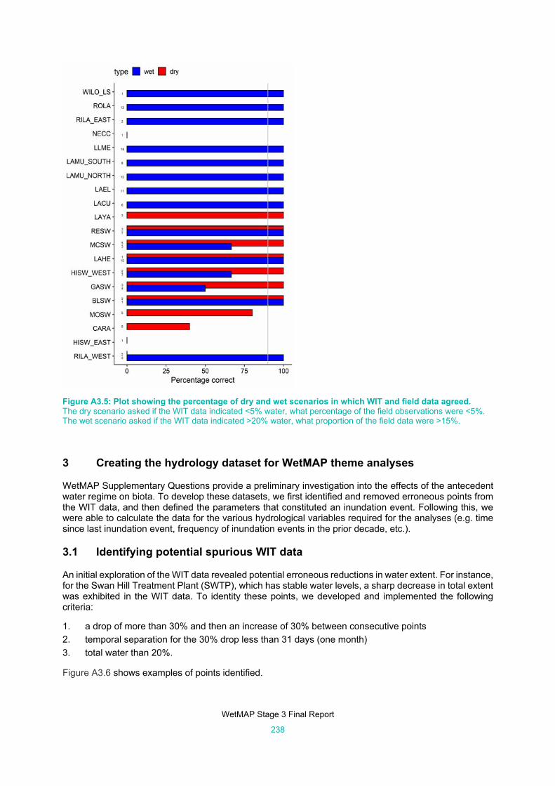
WetMAP Stage 3 Final Report
238
Figure A3.5: Plot showing the percentage of dry and wet scenarios in which WIT and field data agreed. The dry scenario asked if the WIT data indicated <5% water, what percentage of the field observations were <5%. The wet scenario asked if the WIT data indicated >20% water, what proportion of the field data were >15%.
3 Creating the hydrology dataset for WetMAP theme analyses
WetMAP Supplementary Questions provide a preliminary investigation into the effects of the antecedent water regime on biota. To develop these datasets, we first identified and removed erroneous points from the WIT data, and then defined the parameters that constituted an inundation event. Following this, we were able to calculate the data for the various hydrological variables required for the analyses (e.g. time since last inundation event, frequency of inundation events in the prior decade, etc.).
3.1 Identifying potential spurious WIT data
An initial exploration of the WIT data revealed potential erroneous reductions in water extent. For instance, for the Swan Hill Treatment Plant (SWTP), which has stable water levels, a sharp decrease in total extent was exhibited in the WIT data. To identity these points, we developed and implemented the following criteria:
1. a drop of more than 30% and then an increase of 30% between consecutive points
2. temporal separation for the 30% drop less than 31 days (one month)
3. total water than 20%.
Figure A3.6 shows examples of points identified.

WetMAP Stage 3 Final Report
239
Figure A3.6: Plot showing potentially erroneous points (red dots). Panel only shows wetlands in which potential erroneous observations (red dots) might exist. Note that only a subset of the wetlands has been shown.
3.2 Creating the hydrology dataset
Following removal of spurious data, we created daily hydrological profiles for all wetlands. We used the following steps for this process, using the hydrology dataset:
1. We removed all possible erroneous points identified by the method described in the previous subsection.
2. We filled in daily gaps between sampling events (weighted average interpolation).
3. We added in total water (WET + WATER) for each sampling date.
4. We interpolated total water for days not sampled by using the weighted average between the previous and next sampling days (i.e. we assumed a linear slope between sampling observations).
An example of the method is shown in Figure A3.7.
Figure A3.7: Example of the interpolation in the data. Black points are interpolated water values (note that they look like a black line between most blue points); blue dots are actual Geoscience Australia data.

WetMAP Stage 3 Final Report
240
3.3 Defining inundation events
Using the daily hydrology dataset, we next identified unique inundation events. Six options for defining inundation events were identified (Table A3.1). Examples of Option 1 inundation events are shown in Figure A3.8.
Table A3.1: Inundation event options.
Option Wet threshold (extent of inundation) Duration (days)
1 15% 30
2 15% 60
3 20% 30
4 20% 60
5 75% 30
6 75% 60
Figure A3.8: Example of inundations events (option 1) for BLSW site. Top panel shows full profile and bottom shows zoomed in section. Blue lines are inundation events and red lines are dry periods. Distinct inundation events are defined by dry periods.
3.4 Adding in covariates
Using the daily hydrology dataset, we next added in a set of covariates required for the analyses based on a priori predictions about underlying biological hypotheses. Each covariate created is described in Table A3.2.

WetMAP Stage 3 Final Report
241
Table A3.2: Covariates created using the hydrology dataset.
Variable name Long name Description
wet_status wet/dry status on day of sampling
if water is >5% then wet, otherwise it is 'dry'
water_perc_p average of total water in antecedent period (p)
takes the mean of the current day and the p-1 preceding days. P = 1, 30, 90, 180, 360, 1800, 3600, 10,800 days
water_sd_p standard deviation (SD) for total water in antecedent period (p)
takes the SD of the current day and the p-1 preceding days. P = 1, 30, 90, 180, 360, 1800, 3600, 10,800 days
dry_time time since last dry the time since the last dry day at the 5% threshold
wet_time time since last wet the time since the last wet day at the 5% threshold
inun_time_o time since inundation for each option (o)
the time since the end of the last inundation event classified under each option. o = 1,2,3,4,5,6
inun_duration_o
duration of most recent inundation event
the duration of the most recent inundation event based on each option (o). If in a current event, then the duration is the time since the start of that event based on the o = 1,2,3,4,5,6 definition.
inun_longest_p duration of longest inundation events in antecedent period (p)
the maximum duration of all inundation events (o = 1) in which its end date is within the preceding antecedent period (p). If currently in an inundation event, this is not counted.
inun_dur_total_p
duration of all inundation events in antecedent period (p)
the sum of the durations of all inundation events (o = 1) in which its end date is within the preceding antecedent period (p). If currently in an inundation event, this is not counted.
inun_no_s_p number of inundation events under time criteria (s) in antecedent period (p)
the number of inundation events (o = 1) separated by a set time (s) that ends in each antecedent period (p). For inundation events separated by <s, they are combined into a single event. If currently in an event, this is not counted. s = 14,60
4 References
Dunn, B., Lymburner, L., Newey, V., Hicks, A. and Carey, H. (2019). Developing a tool for wetland characterization using fractional cover, tasseled cap wetness and water observations from space. In: Proceedings of IGARSS 2019–2019 IEEE International Geoscience and Remote Sensing Symposium, Yokohama, Japan, 2019, pp. 6095–6097.
R Core Team (20120. R: A language and environment for statistical computing. https://www.R-project.org/

WetMAP Stage 3 Final Report
242
Appendix 4: Species of conservation significance recorded among all surveys in each wetland Table A4.1 Species of conservation significance recorded among all surveys in each wetland.
Species
EP
BC
Act status
Victoria
n Advisory List status
Cara
pugna
Crow
Sw
amp
Neds C
orner Central
Neds C
orner East
Margooya Lagoon
Vinifera F
loodp
lain
Little Lake Heyw
ood
Lake Murphy
Lake Ya
ndo
Woolsh
ed Sw
am
p
Lake Lalbert
Hird S
wam
p
Ganna
warra
Richardso
n’s Lag
oon
Tang T
ang Sw
amp
Mood
ie Sw
amp
Black S
wam
p
Doctors S
wam
p
Gaynor S
wam
p
One T
ree Sw
am
p
Alternanthera nodiflora k x x x x Amaranthus grandiflorus v x Ammannia multiflora v x Amphibromus fluitans V x Asperula gemella r x x x Asperula wimmerana r x x Atriplex holocarpa v x Atriplex lindleyi subsp. lindleyi k x x Austrobryonia micrantha r x x Bergia trimera v x Callitriche umbonata r x
Cardamine lineariloba v x
Cardamine moirensis r x x x x x
Centipeda crateriformis subsp. crateriformis e x x x Centipeda nidiformis r x x Centipeda pleiocephala e x x x Ceratophyllum demersum k x Cullen cinereum e x x Cullen tenax e x Cycnogeton dubium r x Cynodon dactylon var. pulchellus k x x x x x Cyperus bifax v x Cyperus rigidellus e x Diplachne fusca subsp. fusca r x Duma horrida subsp. horrida r x x x x Elacholoma prostrata r x Eleocharis macbarronii k x Eragrostis australasica v x x Eragrostis setifolia v x x x x Eremophila divaricata subsp. divaricata r x Eryngium paludosum v x

WetMAP Stage 3 Final Report
243
Table A4.1 (continued)
Species
EP
BC
Act status
Victoria
n Advisory List status
Cara
pugna
Crow
Sw
amp
Neds C
orner Central
Neds
Corner
East
Margooya Lagoon
Vinifera F
loodp
lain
Little Lake Heyw
ood
Lake Murphy
Lake Ya
ndo
Woolsh
ed Sw
am
p
Lake Lalbert
Hird S
wam
p
Ganna
warra
Richardso
n’s Lag
oon
Tang T
ang Sw
amp
Mood
ie Sw
amp
Black S
wam
p
Doctors S
wam
p
Gaynor S
wam
p
One T
ree Sw
am
p
Glossostigma cleistanthum r x
Glossostigma diandrum v x
Haloragis glauca f. glauca k x
Isolepis australiensis k x x
Lachnagrostis punicea subsp. filifolia r x x x Lepidium fasciculatum k x Lepidium pseudohyssopifolium k x x Maireana cheelii V v x Malacocera tricornis r x Marsilea mutica k x Myriophyllum porcatum V v x Phyllanthus lacunarius v x Picris squarrosa r x
Ranunculus pumilio var. politus k x x x x
Ranunculus sessiliflorus var. pilulifer k x Rorippa eustylis r x x Rumex crystallinus s.s. v x Sclerolaena muricata var. muricata k x x x x x x Sclerolaena muricata var. semiglabra k x Senecio behrianus E e x Senecio cunninghamii var. cunninghamii r x Sida intricata v x Solanum lacunarium v x Stellaria papillata k x Tetragonia moorei k x x Triglochin isingiana k x x Trigonella suavissima r x x Verbena officinalis var. gaudichaudii k x x Wahlenbergia tumidifructa r x Total number of species 12 2 16 9 12 6 10 3 1 2 14 4 2 1 2 2 1 3 2 2
Commonwealth Environment Protection and Biodiversity Conservation Act 1999 (EPBC Act). Conservation status codes (EPBC, VROT): E, e = endangered, V, v = vulnerable, R, r = rare, k = poorly known

WetMAP Stage 3 Final Report
244
Appendix 5: Summary of model selection for wetland plant species richness, cover, lignum and tree tip growth and flowering Table A5.1: Fixed effects coefficients, standard errors, z values and p-values for a generalised Poisson linear mixed model exploring the influence of water regime treatment and time of year on the richness of native wetland plant species groups (KEQ 1).
Species group
Fixed effects Estimate S.E. z value Pr(>|z|)
All wetland species
(Intercept) 1.65 0.16 10.45 <0.001 Treatment.Drawdown.natural.inundation 0.33 0.09 3.74 <0.001 Treatment.Drawdown.ewater 0.54 0.06 9.61 <0.001 Treatment.Inundated.ewater 0.44 0.09 4.65 <0.001 Time.of.Year Dec-Feb –0.15 0.06 –2.67 0.01 Time.of.Year Mar-May –0.37 0.07 –5.43 <0.001
Aquatic species (Intercept) –1.11 0.26 –4.32 <0.001
Treatment.Drawdown.natural.inundation 1.15 0.21 5.50 <0.001 Treatment.Drawdown.ewater 1.45 0.14 10.28 <0.001 Treatment.Inundated.ewater 1.75 0.19 9.18 <0.001 Time.of.Year Dec-Feb –0.18 0.13 –1.34 0.18 Time.of.Year Mar-May –0.28 0.18 –1.60 0.11
Mudflat species (Intercept) –0.17 0.28 –0.61 0.54
Treatment.Drawdown.natural.inundation 0.35 0.22 1.63 0.10 Treatment.Drawdown.ewater 0.87 0.11 7.72 <0.001 Treatment.Inundated.ewater –0.26 0.24 –1.06 0.29 Time.of.Year Dec-Feb –0.47 0.14 –3.30 <0.001 Time.of.Year Mar-May –0.61 0.13 –4.61 <0.001
Seasonally inundated/ immersed species
(Intercept) 0.96 0.15 6.52 <0.001 Treatment.Drawdown.natural.inundation 0.18 0.11 1.68 0.09 Treatment.Drawdown.ewater 0.23 0.08 2.78 0.01 Treatment.Inundated.ewater 0.02 0.16 0.10 0.92 Time.of.Year Dec-Feb –0.10 0.08 –1.23 0.22 Time.of.Year Mar-May –0.30 0.10 –3.12 0.00

WetMAP Stage 3 Final Report
245
Table A5.2: Model selection results for models exploring the influence of hydrological and weather predictors on the richness of native wetland species groups (SQ 1). For total native wetland species richness, richness of damp species and richness of seasonally inundated species, output is from generalised additive mixed models. For aquatic species and mudflat species richness, output is from zero-inflated mixed-effects model.
Species group
Variable AICc Delta Weight
All wetland species
Time since inundated 460.6 0.00 1 Inundation duration (in the prior 10 years) 517.4 56.85 0 Null 534.9 74.32 0 Total rainfall (in the prior 3 months) 534.9 74.35 0 Length of most recent inundation event 539.9 79.31 0 Temperature (average daily maximum in the prior 3 months) 540.1 79.55 0
Aquatic species
Inundation duration (in the prior 10 years) 1064.5 0 1 Total rainfall (in the prior 3 months) 1084.3 19.77 0 Temperature (average daily maximum in the prior 3 months) 1084.9 20.41 0 Null 1097.3 32.81 0 Number of inundation events (in the prior 10 years) 1097.9 33.4 0 Length of most recent inundation event 1098.5 33.98 0
Table A5.2 (continued): Model selection results for models exploring the influence of hydrological and weather predictors on the richness of native wetland species groups (SQ 1). For total native wetland species richness, richness of damp species and richness of seasonally inundated species, output is from generalised additive mixed models. For aquatic species and mudflat species richness, output is from zero-inflated mixed-effects model.
Species group
Variable AICc Delta Weight
Dampland species
Inundation duration (in the prior 10 years) 1812.5 0 1.00 Inundation duration (in the prior 10 years )*Time of Year 1825.0 12.46 0.00 Temperature (average daily maximum in the prior 3 months) 1827.2 14.64 0.00 Null 1832.0 19.44 0.00 Time since inundated 1828.3 15.82 0.00 Length of most recent inundation event 1831.1 18.59 0.00 Total rainfall (in the prior 3 months) 1832.6 20.11 0.00 Number of inundation events (in the prior 10 years ) 1828.5 16.02 0.00
Seasonally inundated species
Number of inundation events (in the prior 10 years ) 1681.2 0 0.36 Null 1681.5 0.35 0.30 Length of most recent inundation event 1683.3 2.11 0.12 Time since inundated 1684.6 3.46 0.06 Total rainfall (in the prior 3 months) 1684.7 3.57 0.06 Temperature (average daily maximum in the prior 3 months) 1685.5 4.29 0.04 Inundation duration (in the prior 10 years ) 1685.6 4.47 0.03
Mudflat species
Number of inundation events (in the prior 10 years) + Temperature (average daily maximum in the prior 3 months) + Total rainfall (in the prior 3 months)
380.4 0 0.52
Number of inundation events (in the prior 10 years) + Temperature (average daily maximum in the prior 3 months)
381.4 1.01 0.31
Number of inundation events (in the prior 10 years) + Total rainfall (in the prior 3 months)
383.1 2.7 0.13
Number of inundation events (in the prior 10 years) 386.8 6.36 0.02 Temperature (average daily maximum in the prior 3 months) 392.6 12.19 0 Total rainfall (in the prior 3 months) 393.6 13.19 0 Null 397.8 17.37 0

WetMAP Stage 3 Final Report
246
Table A5.3: Fixed effects coefficients, standard errors, z values and p-values for an ordinal (cumulative link) mixed model exploring the influence of water regime treatment and time of year on the cover of native wetland species groups (KEQ 2).
Species group Fixed effects Estimate S.E. z value Pr(>|z|) All wetland species Treatment.Drawdown.natural.inundation 1.88 0.55 3.44 <0.001
Treatment.Drawdown.ewater 1.66 0.28 5.95 <0.001 Treatment.Inundated.ewater 0.13 0.47 0.27 0.79 Time.of.Year Dec-Feb 0.36 0.30 1.18 0.24
Aquatic species Treatment.Drawdown.natural.inundation 2.05 0.49 4.20 <0.001 Treatment.Drawdown.ewater 2.52 0.30 8.53 <0.001 Treatment.Inundated.ewater 2.13 0.47 4.50 <0.001 Time.of.Year Dec-Feb –0.68 0.30 –2.30 0.02 Time.of.Year Mar-May –0.16 0.36 –0.43 0.67
Mudflat species Treatment.Drawdown.natural.inundation 1.40 0.53 2.65 0.01 Treatment.Drawdown.ewater 1.65 0.30 5.53 <0.001 Treatment.Inundated.ewater –0.51 0.59 –0.87 0.39 Time.of.Year Dec-Feb –1.40 0.33 –4.20 <0.001 Time.of.Year Mar-May –0.96 0.38 –2.51 0.01
Seasonally inundated/ immersed species
Time.of.Year Dec-Feb 0.53 0.27 1.99 0.05 Time.of.Year Mar-May –0.38 0.35 –1.09 0.28
Table A5.4 Model selection results for models exploring the influence of hydrological and weather predictors on the cover of native wetland species groups (SQ 2). Output is from generalised additive mixed models (GAMMs). For aquatic species and mudflat species, a hurdle model approach was taken; GAMM results were for conditional probabilities only (dataset with zero cover values excluded) and binomial models were also run on the corresponding presence/absence dataset.
Species groups Variable AICc Delta Weight
All wetland species Null 1226.5 0.00 0.459 Total rainfall (in the prior 3 months) 1228.5 1.98 0.170 Temperature (average daily maximum in the prior 3 months) 1229.0 2.53 0.129 Length of most recent inundation event 1230.1 3.60 0.076 Time since inundated 1230.5 3.96 0.063 Inundation duration (in the prior 10 years) 1230.9 4.36 0.052 Number of inundation events (in the prior 10 years) 1230.9 4.38 0.051
Aquatic species Inundation duration (in the prior 10 years) 771.9 0.00 0.989
Null 782.7 10.81 0.004 Time since inundated 783.3 11.38 0.003 Temperature (average daily maximum in the prior 3 months) 785.7 13.82 0.001 Total rainfall (in the prior 3 months) 785.7 13.86 0.001 Length of most recent inundation event 786.4 14.51 0.001 Number of inundation events (in the prior 10 years) 787.1 15.17 0.001
Mudflat species Temperature (average daily maximum in the prior 3 months) 482.8 0.00 0.723
Total rainfall (in the prior 3 months) 485.4 2.56 0.201 Null 488.8 6.01 0.036 Time since inundated 490.2 7.37 0.018 Length of most recent inundation event 490.8 7.97 0.013 Inundation duration (in the prior 10 years) 492.8 10.03 0.005 Number of inundation events (in the prior 10 years) 493.4 10.64 0.004
Seasonally inundated species
Inundation duration (in the prior 10 years) 921.3 0.00 0.469 Length of most recent inundation event 922.8 1.56 0.215 Total rainfall (in the prior 3 months) 923.6 2.30 0.148 Temperature (average daily maximum in the prior 3 months) 924.3 2.98 0.106 Null 925.8 4.51 0.049 Number of inundation events (in the prior 10 years) 929.7 8.41 0.007 Time since inundated 929.9 8.60 0.006

WetMAP Stage 3 Final Report
247
Table A5.5: Fixed effects coefficients, standard errors, z values and p-values for an ordinal (cumulative link) mixed model exploring the influence of water regime treatment and time of year on native and introduced terrestrial species cover (KEQ 3).
Species group Fixed effects Estimate S.E. z value Pr(>|z|) Native species Treatment.Drawdown.natural.inundation –1.82 0.72 –2.52 0.01
Treatment.Drawdown.ewater –1.15 0.37 –3.11 0.00 Treatment.Inundated.ewater –3.31 0.76 –4.33 <0.001 Time.of.Year Dec-Feb –0.25 0.37 –0.68 0.50 Time.of.Year Mar-May –1.49 0.57 –2.62 0.01
Introduced species Treatment.Drawdown.natural.inundation –2.46 0.52 –4.76 <0.001
Treatment.Drawdown.ewater –0.76 0.27 –2.83 0.00 Treatment.Inundated.ewater –2.79 0.57 –4.90 <0.001 Time.of.Year Dec-Feb –1.06 0.30 –3.51 <0.001 Time.of.Year Mar-May –0.18 0.35 –0.52 0.60
Table A5.6: Fixed effects coefficients, standard errors, z values and p-values for a linear mixed model exploring the influence of water regime treatment and time of year on lignum condition (KEQ 4).
Fixed effects Estimate S.E. df t value Pr(>|t|) (Intercept) 78.56 7.80 12.41 10.08 <0.001 Treatment.Drawdown.natural.inundation 4.02 11.11 128.88 0.36 0.72 Treatment.Drawdown.ewater 9.91 5.89 117.23 1.68 0.10 Treatment.Inundated.ewater 4.98 8.69 150.38 0.57 0.57 Time.of.Year Dec-Feb 6.64 5.65 116.60 1.17 0.24 Time.of.Year Mar-May –3.33 8.62 104.62 -0.39 0.70 Table A5.7: Model selection results for lignum condition (SQ 4). Model AICc Delta Weight
Total days inundated in the prior 10 years 618.7 0.00 0.95 Total days inundated in the prior 10 years + Time since inundation 624.6 5.88 0.05 Time since inundation 642.4 23.73 0.00 Null 644.9 26.16 0.00 Rainfall in the prior 10 years 646.3 27.54 0.00 Table A5.8: Summary of ordinal regression examining the effects of hydrological treatment and rainfall on tip growth scores for River Red Gum and Black Box (KEQ 5). Note that River Red Gum data came from wetlands with three different hydrological treatments, whereas Black Box data came from wetlands with two hydrological treatments. The hydrological treatment terms are interpreted in response to the Drawdown – e-water treatment, i.e. here a significant p-value and positive estimate for Drawdown – natural inundation indicate that lower tip growth scores for River Red Gum are likely at watered sites.
Species Variable Estimate SE z p River Red Gum Treat(Drawdown – natural inundation) 1.28 0.39 3.30 <0.001
Treat(Dry) –1.81 0.26 –6.92 <0.001 Rainfall –0.02 0.00 –6.64 <0.001 Temperature 0.13 0.02 5.78 <0.001
Black Box Treat(Dry) –1.42 0.31 –4.65 0.00 Rainfall –0.02 0.00 –4.61 0.00 Temperature 0.02 0.02 0.93 0.35

WetMAP Stage 3 Final Report
248
Table A5.9: Summary of ordinal regression examining the effects of hydrological treatment and rainfall on flowering scores for River Red Gum and Black Box (KEQ 5). Note that both River Red Gum and Black Box data came from wetlands with three different hydrological treatments.
Species Variable Estimate SE z p River Red Gum Treat(Drawdown – natural inundation) 1.11 0.42 2.67 0.01
Treat(Dry) 0.58 0.27 2.19 0.03 Rainfall 0.00 0.00 –1.56 0.12 Temperature 0.02 0.02 0.91 0.36
Black Box Treat(Dry) –0.67 0.36 –1.85 0.06 Rainfall –0.02 0.00 –5.20 <0.001 Temperature –0.02 0.02 –0.97 0.33

WetMAP Stage 3 Final Report
249
Appendix 6: Supporting information for interpreting frog monitoring results
Figure A6.1: Number of waterbodies within surrounding 1 km of focal wetlands.

WetMAP Stage 3 Final Report
250
Table A6.1: Summary of species detected at individual transects at each wetland using AudioMoth loggers and audiovisual surveys, 2018–2019. Values of 0 and dark-green fill highlight when a species was recorded as absent using both methods, values of 2 and light-green fill highlight when a species was recorded as present using both methods, values of 1 and red fill highlight when audiovisual surveys detected a species and AudioMoth acoustic logger classifiers did not, and values of –1 and orange fill when a species was detected on AudioMoth acoustic logger classifiers but not in audiovisual surveys. Note that data were not available for all AudioMoth loggers. Species codes: Crin parin Crinia parinsignifera, Crin sig C. signifera, Crin sloan C. sloanei, Lim dumer Limnodynastes dumerilii, Lim fletch L. fletcheri, Lim tasman L. tasmaniensis, Lit ewing Litoria ewingii, Lit peron L. peronii
Wetland
Species:
Transect
Crin parin
Crin sig
Crin sloan
Lim dumer
Lim fletch
Lim tasman
Lit ewing
Lit peron
Black Swamp Black Swamp 1 1 1 0 2 0 2 0 1
Black Swamp 2 0 0 0 –1 0 2 0 1
Carapugna Carapugna 2 0 0 0 2 0 2 0 2
Carapugna 3 0 0 0 2 0 2 0 1
Cowanna Billabong Cowanna Billabong 1 1 0 0 0 1 –1 0 2
Cowanna Billabong 2 –1 0 0 –1 2 –1 0 2
Cowanna Billabong 3 1 0 0 1 2 2 0 2
Cowanna Billabong 4 1 0 0 2 2 –1 0 2
Crow Swamp Crow Swamp 1 0 –1 0 2 0 2 0 0
Crow Swamp 2 1 2 0 2 0 2 0 0
Ducksfoot Lagoon Ducksfoot Lagoon 2 2 0 0 2 1 2 0 2
Gaynor Swamp Gaynor Swamp 1 1 0 0 2 0 2 0 0
Gaynor Swamp 2 1 1 0 2 0 2 0 1
Gaynor Swamp 3 1 1 0 2 0 2 0 0
Gaynor Swamp 4 1 1 0 1 0 2 0 1
Kings Billabong Kings Billabong 1 1 –1 0 1 0 2 0 2
Kings Billabong 2 1 0 0 0 0 –1 0 2
Kings Billabong 3 1 0 0 0 0 2 0 2

WetMAP Stage 3 Final Report
251
Wetland
Species:
Transect
Crin parin
Crin sig
Crin sloan
Lim dumer
Lim fletch
Lim tasman
Lit ewing
Lit peron
Kings Billabong 5 0 0 0 –1 0 –1 0 2
Kinnairds Wetland Kinnairds Wetland 1 2 2 0 1 0 2 0 2
Kinnairds Wetland 2 2 0 0 1 –1 2 0 2
Kinnairds Wetland 3 1 0 0 1 1 2 0 1
Lake Murphy Lake Murphy 1 1 2 –1 2 2 2 0 2
Lake Murphy 2 2 1 0 2 2 2 0 –1
Lake Murphy 3 2 1 –1 2 –1 2 0 –1
Little Lake Meran Little Lake Meran 1 1 0 0 2 0 2 0 2
Nyah Floodplain Nyah Floodplain 1 0 0 0 0 2 –1 0 2
Nyah Floodplain 2 0 0 0 0 2 2 0 2
Nyah Floodplain 3 0 0 –1 –1 2 –1 0 2
Nyah Floodplain 4 0 0 0 0 1 2 0 2
Richardson’s Lagoon Richardson’s Lagoon 1 0 1 0 0 0 –1 0 1
Richardson’s Lagoon 2 0 1 0 –1 1 –1 0 2
Richardson’s Lagoon 3 0 0 0 0 0 2 0 1
Richardson’s Lagoon 4 1 1 0 –1 0 –1 0 1
Richardson’s Lagoon 5 1 1 0 1 1 2 0 1
Wallpolla Horseshoe Lagoon Wallpolla Horseshoe Lagoon 1 2 –1 0 1 2 2 0 2
Wallpolla Horseshoe Lagoon 2 2 2 0 0 2 –1 0 2
Wallpolla Horseshoe Lagoon 4 2 0 0 2 2 2 0 2
Wirra-Lo Duck Creek Wirra-Lo Duck Creek 1 2 0 0 2 2 2 0 2
Wirra-Lo Lignum Swamp North Wirra-Lo Lignum Swamp Nth 1 2 2 0 2 2 2 –1 2

WetMAP Stage 3 Final Report
252
Table A6.2: Summary of model selection for abundances of all frogs.
Variable AICc Delta Weight
Hydrology Wet proportion (30 days) 133 0 0.43
Wet proportion (90 days) 133.1 0.14 0.41
Wet proportion (day of sampling) 135.5 2.53 0.12
Wet proportion (180 days) 139.1 6.09 0.02
No. waterbodies within 1 km 139.3 6.31 0.02
Null 140 7.00 0.01
Wet proportion (360 days) 142.9 9.87 0.00
Wet proportion (30 days) + No. waterbodies within 1 k
143.4 10.44 0.00
Water quality Null 105 0 0.99
Conductivity 119.8 14.86 0.01
Habitat Null 147.3 0.00 0.62
Tall emergent 149.6 2.28 0.20
Short herbs/grasses 151.7 4.41 0.07
Bare ground 151.8 4.53 0.07
Short emergent 152.6 5.31 0.04

WetMAP Stage 3 Final Report
253
Table A6.3: Summary of model selection for abundances of Crinia parinsignifera.
Variable AICc Delta Weight
Hydrology Wet proportion (30 days) 125.8 0 0.41
Wet proportion (day of sampling) 126 0.21 0.37
Null 127.7 1.89 0.16
No. wetlands within 1 km 129.2 3.44 0.07
Wet proportion (90 days) 130.8 5.05 0.03
Wet proportion (180 days) 132.9 7.12 0.01
Wet proportion (360 days 133.2 7.44 0.01
Wet proportion (30 days) + No. waterbodies within 1 k
136.5 10.68 0.00
Water quality Null 113.2 0 1.00
Conductivity 127 13.83 0.00
Habitat Null 136.6 0 0.81
Short emergent 141.5 4.93 0.07
Short herbs and grasses 141.8 5.23 0.06
Tall emergent 142.7 6.07 0.04
Bare ground 143.3 6.69 0.02

WetMAP Stage 3 Final Report
254
Table A6.4: Summary of model selection for abundance of Limnodynastes dumerilii.
Variable AICc Delta Weight
Hydrology Wet proportion (90 days) 94.9 0 0.80
Wet proportion (30 days) 99.4 4.51 0.08
Null 99.8 4.87 0.07
Wet proportion (day of sampling) 101.5 6.63 0.03
Wet proportion (180 days) 102.5 7.64 0.02
Wet proportion (360 days) 106 11.1 0.00
No. waterbodies within 1 km 106.7 11.82 0.00
Wet proportion (90 days) + No. waterbodies within 1 km 113.2 18.28 0.00
Water quality Null 90.2 0 1.00
Conductivity 106.9 16.73 0.00
Habitat Tall emergent 99.6 0 0.87
Null 105.1 5.56 0.05
Bare ground 105.3 5.76 0.05
Short emergent 107.3 7.79 0.02
Short herbs/grasses 110.5 10.94 0.00
Full Tall emergent 93.4 0 0.48
Wet proportion (90 days) 93.9 0.51 0.37
Wet proportion (90 days) + Tall emergent 96.6 3.23 0.09
Null 97.5 4.12 0.06
Wet proportion (90 days)*Complexity + Tall emergent 115.6 22.26 0.00

WetMAP Stage 3 Final Report
255
Table A6.5: Summary of model selection for abundances of Limnodynastes tasmaniensis.
Variable AICc Delta Weight
Hydrology Wet proportion (90 days) 125.1 0 0.93
Wet proportion (90 days) + No. waterbodies within 1 km 131.5 6.44 0.04
Wet proportion (180 days) 133.3 8.22 0.02
Wet proportion (30 days) 135 9.93 0.01
Wet proportion (day of sampling) 135.6 10.54 0.09
Null 135.9 10.83 0.00
Wet proportion (360 days) 137.4 12.28 0.00
No. waterbodies within 1 km 140.7 15.55 0.00
Water quality Null 112.6 0 1.00
Conductivity 128.8 16.14 0.00
Habitat Tall emergent 135.3 0 0.74
Short emergent 138.1 2.87 0.18
Null 142.2 6.92 0.02
Short herbs/grasses 143.8 8.54 0.01
Bare ground 148.3 13.06 0.00
Full Wet proportion (90 days) 122.9 0 0.53
Wet proportion (90 days) + Tall emergent 123.7 0.82 0.35
Tall emergent 126 3.18 0.11
Null 131.9 9.02 0.01
Wet proportion (90 days)*Complexity + Tall emergent 139.9 17.05 0.00

WetMAP Stage 3 Final Report
256
Table A6.6: Summary of model selection for abundances of Litoria peronii.
Variable AICc Delta Weight
Hydrology Null 125.7 0 0.48
Wet proportion (day of sampling) 127.5 1.85 0.19
Wet proportion (30 days) 128.1 2.38 0.14
No. waterbodies within 1 km 128.4 2.76 0.12
Wet proportion (90 days) 131.8 6.17 0.2
Wet proportion (180 days) 132.4 6.7 0.02
Wet proportion (360 days) 132.5 6.8 0.02
Water quality Null 110.3 0 0.98
Conductivity 119.2 8.88 0.02
Habitat Null 137.4 0 0.60
Bare ground 138.8 1.38 0.30
Short emergent 142.7 5.26 0.04
Short herbs/grasses 143.6 6.19 0.03
Tall emergent 143.9 6.44 0.02

WetMAP Stage 3 Final Report
257
Appendix 7: Waterbird species, Guild assignment and conservation status Table A7.1: Waterbird species recorded at watered wetlands during WetMAP Phase 1, including the guild each is assigned to (defined largely by foraging behaviour, Rogers et al. 2019) and its conservation status. Migratory species are listed as matters of national significance under the EPBC Act and some of these species are also listed under threatened species categories.
Common name Species name Guild Status in Victorian
Advisory List Status under FFG Act Status under EPBC Act
Common Sandpiper Actitis hypoleucos Shorebirds Migratory
Chestnut Teal Anas castanea Shallow Waterfowl
Grey Teal Anas gracilis Shallow Waterfowl
Australasian Shoveler Anas rhynchotis Shallow Waterfowl Vulnerable
Pacific Black Duck Anas superciliosa Shallow Waterfowl
Australasian Darter Anhinga novaehollandiae Swimming Piscivores
Magpie Goose Anseranas semipalmata Shallow Waterfowl Near-threatened Listed
Eastern Cattle Egret Ardea ibis Large Waders
Intermediate Egret Ardea intermedia Large Waders Endangered Listed
Great Egret Ardea modesta Large Waders Listed Listed
White-necked Heron Ardea pacifica Large Waders
Hardhead Aythya australis Deep Waterfowl Vulnerable
Musk Duck Biziura lobata Deep Waterfowl Vulnerable
Australasian Bittern Botaurus poiciloptilus Skulkers Endangered Listed Endangered
Sharp-tailed Sandpiper Calidris acuminata Shorebirds Migratory
Curlew Sandpiper Calidris ferruginea Shorebirds Migratory
Red-necked Stint Calidris ruficollis Shorebirds Migratory

WetMAP Stage 3 Final Report
258
Common name Species name Guild Status in Victorian
Advisory List Status under FFG Act Status under EPBC Act
Long-toed Stint Calidris subminuta Shorebirds Near-threatened Migratory
Double-banded Plover Charadrius bicinctus Shorebirds
Red-capped Plover Charadrius ruficapillus Shorebirds
Australian Wood Duck Chenonetta jubata Shallow Waterfowl
Whiskered Tern Chlidonias hybrida Terns
White-winged Black Tern Chlidonias leucopterus Terns Near-threatened Migratory
Banded Stilt Cladorhynchus leucocephalus Shorebirds
Black Swan Cygnus atratus Deep Waterfowl
White-faced Heron Egretta novaehollandiae Large Waders
Black-fronted Dotterel Elseyornis melanops Shorebirds
Red-kneed Dotterel Erythrogonys cinctus Shorebirds
Eurasian Coot Fulica atra Deep Waterfowl
Latham's Snipe Gallinago hardwickii Skulkers Near-threatened Migratory
Dusky Moorhen Gallinula tenebrosa Shallow Waterfowl
Buff-banded Rail Gallirallus philippensis Skulkers
Brolga Grus rubicunda Large Waders Vulnerable Listed
White-headed Stilt Himantopus himantopus Shorebirds
Australian Little Bittern Ixobrychus dubius Skulkers Endangered Listed
Black-tailed Godwit Limosa limosa Shorebirds Migratory
Pink-eared Duck Malacorhynchus membranaceus Shallow Waterfowl
Blue-billed Duck Oxyura australis Deep Waterfowl Endangered Listed

WetMAP Stage 3 Final Report
259
Common name Species name Guild Status in Victorian
Advisory List Status under FFG Act Status under EPBC Act
Australian Pelican Pelecanus conspicillatus Swimming Piscivores
Great Cormorant Phalacrocorax carbo Swimming Piscivores
Little Black Cormorant Phalacrocorax sulcirostris Swimming Piscivores
Pied Cormorant Phalacrocorax varius Swimming Piscivores Near-threatened
Little Pied Cormorant Phalacrocorax melanoleucos Swimming Piscivores
Yellow-billed Spoonbill Platalea flavipes Large Waders
Royal Spoonbill Platalea regia Large Waders Near-threatened
Glossy Ibis Plegadis falcinellus Large Waders
Pacific Golden Plover Pluvialis fulva Shorebirds Migratory
Great Crested Grebe Podiceps cristatus Swimming Piscivores
Hoary-headed Grebe Poliocephalus poliocephalus Swimming Piscivores
Australasian Swamphen Porphyrio melanotus Skulkers
Australian Spotted Crake Porzana fluminea Skulkers
Spotless Crake Porzana tabuensis Skulkers
Red-necked Avocet Recurvirostra novaehollandiae Shorebirds
Freckled Duck Stictonetta naevosa Shallow Waterfowl Endangered Listed
Australasian Grebe Tachybaptus novaehollandiae Swimming Piscivores
Australian Shelduck Tadorna tadornoides Shallow Waterfowl
Australian White Ibis Threskiornis molucca Large Waders
Straw-necked Ibis Threskiornis spinicollis Large Waders
Wood Sandpiper Tringa glareola Shorebirds Migratory

WetMAP Stage 3 Final Report
260
Common name Species name Guild Status in Victorian
Advisory List Status under FFG Act Status under EPBC Act
Common Greenshank Tringa nebularia Shorebirds Migratory
Marsh Sandpiper Tringa stagnatilis Shorebirds Vulnerable Migratory
Masked Lapwing Vanellus miles Shorebirds
EPBC Act = Commonwealth Environment Protection and Biodiversity Conservation Act 1999, FFG Act = Victorian Flora and Fauna Guarantee Act 1988

WetMAP Stage 3 Final Report
261
Appendix 8: Supplementary Questions on the WetMAP bird theme Table A8.1: Supplementary Questions of the WetMAP bird theme. Further background on these questions is given in Rogers (2019). Four of these questions are considered in this report.
SQs Additional data/approaches required
Time frame
1. How do waterbird abundance and species richness change with water level in watered wetlands? (SQ 1 in this report)
Water depth from depth sensors, bathymetry of wetlands
Preliminary results by end of 2019–2020
2. How do waterbird abundance and species richness change with spatial extent of wetland inundation? (SQ3 in this report)
Wetland extent data provided from GA (wetland insight tool)
Preliminary results by end of 2019–2020
3. How do waterbird abundance and species richness change with duration of flooding in watered wetlands? (SQ 2 in this report)
Wetland extent data provided from GA (wetland insight tool)
Preliminary results by end of 2019–2020
4. Are waterbird abundance and species richness at wetlands affected by availability of alternative habitats in the same region?
Assess whether there are negative correlations between counts at paired sites, which would be consistent with movement between the two sites. Wetland extent data provided from satellite imagery at a regional scale Habitat assessments of nearby wetlands
Further experimental design and site selection
Preliminary result with 2–
5 years
5. Are waterbird abundance and species richness affected by continental rainfall patterns, and water availability in the Australian landscape? (SQ4 in this report)
Victorian Biodiversity Atlas records; Victorian Summer Waterfowl Counts; BirdLife Australia database records; rainfall records and water extent data from satellite imagery
2–5 years
Model continually refined as new data are collected
6. Do waterbirds that use WetMAP bird monitoring sites breed elsewhere (local, regional, continental)?
Tag selected waterfowl species with GSM tags at non-breeding sites. GPS-precision locations plus accelerometer data to be used to identify breeding locations, species to be determined.
2–5 years
7. What are the habitat characteristics where waterbirds are breeding?
Characterise all breeding sites using aerial/satellite imagery; field trips to accessible sites for more complete habitat description. Review of literature and other data sets.
2–5 years
8. Do waterbird species show site fidelity to wetlands?
Assess how many tagged birds return to same site to breed
2–5 years

WetMAP Stage 3 Final Report
262
SQs Additional data/approaches required
Time frame
across multiple seasons, species to be determined.
9. How often do Victorian waterbird species breed?
Deploy tags on non-breeding waterbirds (selected waterfowl species) and assess how many nest in the following breeding season (using GPS-precision location and accelerometer data). Carry out study over multiple years to assess whether there is annual variation and the effects of rainfall. Test theory that more birds attempt to breed in wetter years, species to be determined.
5–10 years
10. Was suitable breeding habitat available at watered wetlands?
Water depth from depth sensors, bathymetry of wetlands. Literature review
2–5 years
11. Was the wetland flooded long enough for a breeding attempt?
Literature review, examining other datasets
2–5 years
12. What is the expected lag time between water delivery, zooplankton abundance and waterbird response in watered wetlands?
Analysis of samples collected during the past 3 years of WetMAP fieldwork.
2–5 years
13. What are the water regime requirements (timing and duration) for different waterbird species?
Literature review, examining other datasets
2–5 years
14. What are the local wetland habitat preferences for selected species of waterbirds for feeding, resting and breeding?
Focal study at selected wetlands monitoring bird usage patterns over entire day (e.g. focal scans every 30 min) to determine time spent feeding, resting or breeding in each habitat type. Species selection to be determined. GPS-precision locality data and accelerometer data from satellite tracking data over day and night.
2–5 years
GA = Geoscience Australia
References
Rogers, D. (2019). Project plan: 2019–20 WetMAP bird theme 2019–20 monitoring bird response to environmental water delivery in Victoria. Prepared for Water and Catchments, Department of Environment, Land, Water and Planning, Heidelberg, Victoria.

WetMAP Stage 3 Final Report
263
Appendix 9: Waterbird abundance and diversity Between 2017 and June 2020, WetMAP carried out 267 waterbird counts, in which a total of 931,060 waterbirds were recorded. In total, 71 waterbird species were recorded during WetMAP counts. The maximum totals on a single day, by species, for the wetlands that received environmental water and the other sites that we monitored are presented in Table A9.3. These maxima sum to 188,102 waterbirds observed during the study: 118,944 spread across the 20 wetlands that received environmental water; 64,783 in monitored wastewater treatment plants, and 4375 in sites where we carried out exploratory surveys before deciding to discontinue monitoring (Table A9.1). The total number of birds that used the wetlands over time was probably higher, given the likelihood of turnover of individual birds between site visits.
Species richness and abundance varied considerably between wetlands, and within wetlands from survey to survey (Figure A9.1). Ducks (Shallow and Deep Waterfowl) were the most numerous waterbirds on most wetlands, followed by Swimming Piscivores and Shorebirds; Large Waders and Skulkers were least numerous (Table A9.2). Wetlands that received environmental water held proportionately more Deep Waterfowl, Large Waders and Skulkers than wastewater treatment plants (Table A9.2).
Twenty waterbird species were recorded that are listed as threatened under the FFG Act, the EPBC Act or in the Advisory List of Threatened Vertebrate Fauna in Victoria (Table A9.3). Noteworthy counts included 22 Australasian Bittern (including 16 on Lake Cullen), >24,000 Australasian Shoveler (>50% on Lakes Murphy and Elizabeth), 1086 Blue-billed Duck (mainly on the two wastewater treatment plants), 18 Brolga and 453 Freckled Duck. Migratory shorebirds (listed as a matter of national environmental significance) were recorded on 10 wetlands that received environmental water (mainly Lakes Cullen, Elizabeth and Murphy), and Shepparton and Swan Hill wastewater treatment plants. While hundreds of Shorebirds (mainly Red-necked Stint and Sharp-tailed Sandpiper) were found at the monitored wetlands and treatment plants, no species were found in internationally significant numbers.
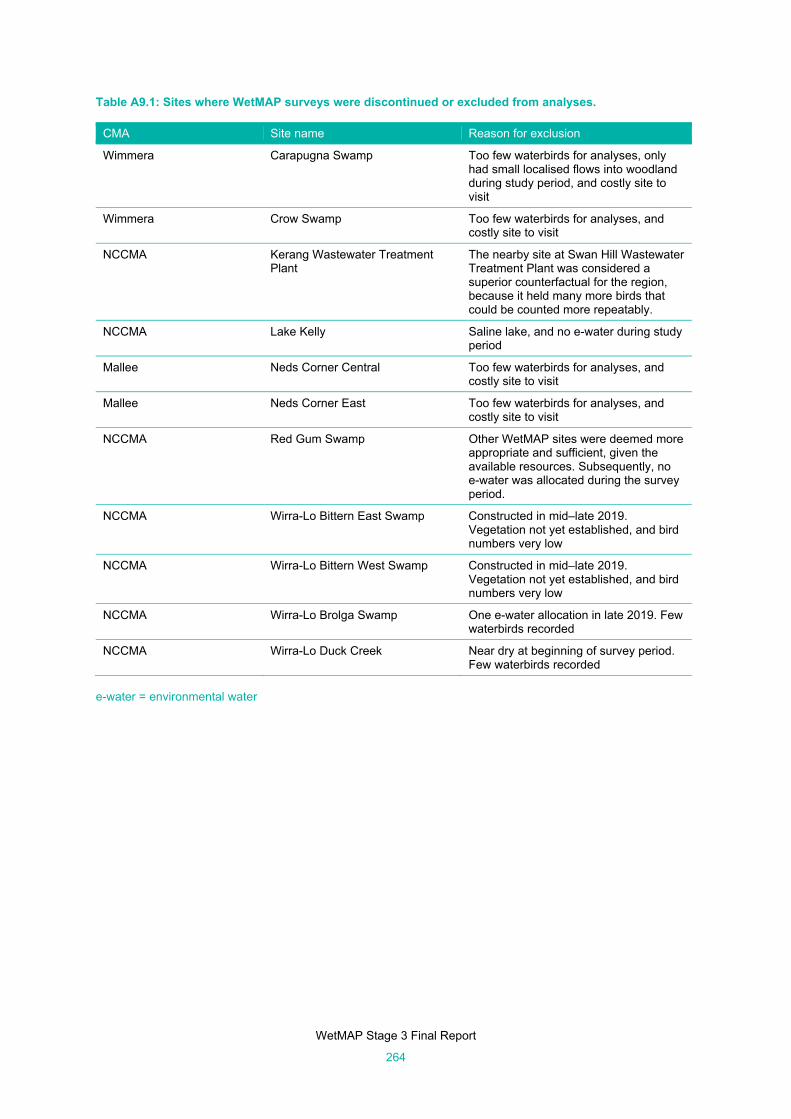
WetMAP Stage 3 Final Report
264
Table A9.1: Sites where WetMAP surveys were discontinued or excluded from analyses.
CMA Site name Reason for exclusion
Wimmera Carapugna Swamp Too few waterbirds for analyses, only had small localised flows into woodland during study period, and costly site to visit
Wimmera Crow Swamp Too few waterbirds for analyses, and costly site to visit
NCCMA Kerang Wastewater Treatment Plant
The nearby site at Swan Hill Wastewater Treatment Plant was considered a superior counterfactual for the region, because it held many more birds that could be counted more repeatably.
NCCMA Lake Kelly Saline lake, and no e-water during study period
Mallee Neds Corner Central Too few waterbirds for analyses, and costly site to visit
Mallee Neds Corner East Too few waterbirds for analyses, and costly site to visit
NCCMA Red Gum Swamp Other WetMAP sites were deemed more appropriate and sufficient, given the available resources. Subsequently, no e-water was allocated during the survey period.
NCCMA Wirra-Lo Bittern East Swamp Constructed in mid–late 2019. Vegetation not yet established, and bird numbers very low
NCCMA Wirra-Lo Bittern West Swamp Constructed in mid–late 2019. Vegetation not yet established, and bird numbers very low
NCCMA Wirra-Lo Brolga Swamp One e-water allocation in late 2019. Few waterbirds recorded
NCCMA Wirra-Lo Duck Creek Near dry at beginning of survey period. Few waterbirds recorded
e-water = environmental water

WetMAP Stage 3 Final Report
265
Figure A9.1: (a) Waterbird richness and (b) Waterbird number observed at wetlands during surveys. The boxplots show mean count per survey, 25 and 75% quantiles, minimum and maximum for each site. Labels on the y-axis are abbreviations for the site names in Tables 9.1 and 9.3. Table A9.2: Comparison of waterbird numbers on wetlands that received environmental water with waterbird numbers on wastewater treatment plants.
Guild
Wetlands with environmental water (n = 239 site visits)
Wastewater treatment plants (n = 28 site visits)
No. of birds
Percentage of
waterbirds
No. of threatened
species
No. of birds
Percentage of waterbirds
No. of threatened
species
Shallow Waterfowl 47,176 38.3% 2 42,156 65.07% 2
Deep Waterfowl 46,437 37.7% 3 8,717 13.46% 3
Swimming Piscivores 10,834 8.8% 0 7,594 11.72% 0
Shorebirds 9,378 7.6% 6 5,093 7.86% 4
Terns 4,047 3.3% 1 951 1.47% 0
Large Waders 3,960 3.2% 4 143 0.22% 2
Skulkers 1,476 1.2% 3 129 0.20% 0
Total 123,308 19 64,783 11

WetMAP Stage 3 Final Report
266
Table A9.3: Maximum counts of waterbirds at monitored WetMAP sites. Species listed as threatened or near-threatened under the EPBC Act, FFG Act or Victorian Advisory List are in boldface.
Species
Black S
wam
p
Gayn
or S
wam
p
Heyw
oo
d’
s Lake
Hird
Sw
amp
Joh
nso
n S
wam
p
Lake C
ullen
Lake E
lizabeth
Little L
ake Meran
Lake M
eran
Lake M
urp
hy
Lake Y
and
o
McD
on
alds S
wam
p
Mo
od
ie Sw
amp
Reed
y Sw
amp
(S
hep
parto
n)
Rich
ardso
n’
s Lag
oo
n
Ro
un
d L
ake
Sh
epp
arton
WW
TP
Sw
an H
ill WW
TP
Vin
ifera Flo
od
plain
Wirra-L
o
Gran
d to
tal
Australasian Bittern 2 16 3 1 22
Australasian Grebe 25 7 43 14 816 2 137 121 3 42 6 95 19 3 20 8 1,361
Australasian Shoveler
8 25 4 247 504 106 750 84 9 142 318 225 2,422
Australian Pelican 232 9 5 2,418 13 15 60 7 2 2 15 11 1 101 2 4 2,897
Australian Pratincole 1 1
Australian Shelduck 15 74 13 2 1,030 254 7 115 1 22 57 16 28 182 739 4 2,559
Australian Spotted Crake
4 7 27 1 2 1 3 45
Australian White Ibis 10 40 20 12 138 87 9 4 38 7 108 9 9 6 3 7 507
Australian Wood Duck
3 713 4 34 5 55 15 8 2 29 9 9 138 219 66 60 1,369
Baillon's Crake 2 2
Banded Stilt 10 15 25
Black Swan 4 65 14 24 7,527 1,227 70 6 1,202 10 32 28 91 311 145 10,756
Black-fronted Dotterel 14 9 12 6 5 14 4 4 19 29 35 5 13 20 189
Black-tailed Godwit 1 1
Black-tailed Native-hen
27 84 348 162 9 59 125 45 254 22 9 52 117 27 1,340
Black-winged Stilt 1,452 25 60 25 2,011 21 50 170 579 134 143 4 28 116 149 3 4,970
Blue-billed Duck 104 58 2 2 1 6 776 137 1,086

WetMAP Stage 3 Final Report
267
Species
Black S
wam
p
Gayn
or S
wam
p
Heyw
oo
d’
s Lake
Hird
Sw
amp
Joh
nso
n S
wam
p
Lake C
ullen
Lake E
lizabeth
Little L
ake Meran
Lake M
eran
Lake M
urp
hy
Lake Y
and
o
McD
on
alds S
wam
p
Mo
od
ie Sw
amp
Reed
y Sw
amp
(S
hep
parto
n)
Rich
ardso
n’
s Lag
oo
n
Ro
un
d L
ake
Sh
epp
arton
WW
TP
Sw
an H
ill WW
TP
Vin
ifera Flo
od
plain
Wirra-L
o
Gran
d to
tal
Brolga 8 3 2 2 3 18
Buff-banded Rail 1 1
Caspian Tern 1 150 1 152
Cattle Egret 3 3
Chestnut Teal 8 2 1 904 12 2 16 3 68 9 3 163 12 59 1,262
Common Greenshank 1 7 1 1 2 1 13
Common Sandpiper 5 5
Curlew Sandpiper 3 1 1 4 9
Darter 5 10 3 3 55 39 11 1 1 3 1 3 135
Double-banded Plover
2 5 7
Dusky Moorhen 2 2 1 2 3 8 1 3 3 1 26
Eastern Great Egret 1 32 13 1 493 1 4 1 14 1 2 1 1 565
Eurasian Coot 13 87 166 10 26,113 1,071 522 5,154 36 7 244 1,179 451 1 35,054
Freckled Duck 8 51 57 2 97 4 41 18 175 453
Glossy Ibis 107 112 96 97 42 36 75 2 1 568
Great Cormorant 9 178 2 615 3 23 8 19 1 5 37 2 3 905
Great Crested Grebe 5 119 4 1 129
Grey Teal 1,050 1,137 508 1,356 11,425 4,106 313 275 6,835 7 751 1,825 210 803 2,375 6,141 565 28 39,710
Gull-billed Tern 4 6 10
Hardhead 7 11 17 48 1,532 12 65 4 204 20 17 167 3,576 2,063 7,743

WetMAP Stage 3 Final Report
268
Species
Black S
wam
p
Gayn
or S
wam
p
Heyw
oo
d’
s Lake
Hird
Sw
amp
Joh
nso
n S
wam
p
Lake C
ullen
Lake E
lizabeth
Little L
ake Meran
Lake M
eran
Lake M
urp
hy
Lake Y
and
o
McD
on
alds S
wam
p
Mo
od
ie Sw
amp
Reed
y Sw
amp
(S
hep
parto
n)
Rich
ardso
n’
s Lag
oo
n
Ro
un
d L
ake
Sh
epp
arton
WW
TP
Sw
an H
ill WW
TP
Vin
ifera Flo
od
plain
Wirra-L
o
Gran
d to
tal
Hoary-headed Grebe 47 332 78 2 1,460 370 461 2 980 7 6 166 6,507 862 6 1 11,287
Intermediate Egret 2 4 1 7
Latham's Snipe 1 6 1 8
Little Bittern 3 3
Little Black Cormorant
7 48 372 1 34 10 15 1 2 46 3 39 11 589
Little Curlew 1 1
Little Egret 3 1 4
Little Pied Cormorant 6 85 18 36 286 10 3 32 9 3 21 3 1 1 514
Long-toed Stint 1 1
Magpie Goose 3 8 11
Marsh Sandpiper 1 3 30 8 2 8 54 106
Masked Lapwing 10 42 20 2 139 90 7 28 84 3 43 20 7 13 128 43 2 8 689
Musk Duck 2 1 10 3 5 2 79 102
Nankeen Night Heron 1 1
Pacific Black Duck 6 164 63 116 11 72 0 32 12 331 24 127 105 39 70 278 74 36 1,560
Pacific Golden Plover 3 3
Pied Cormorant 2 50 1 4 57
Pink-eared Duck 24 2 2,110 2,283 437 1,260 6 712 22,377 8,726 37,937
Purple Swamphen 3 3 6 63 4 14 12 4 8 117
Red-capped Plover 49 260 66 2 23 70 79 549
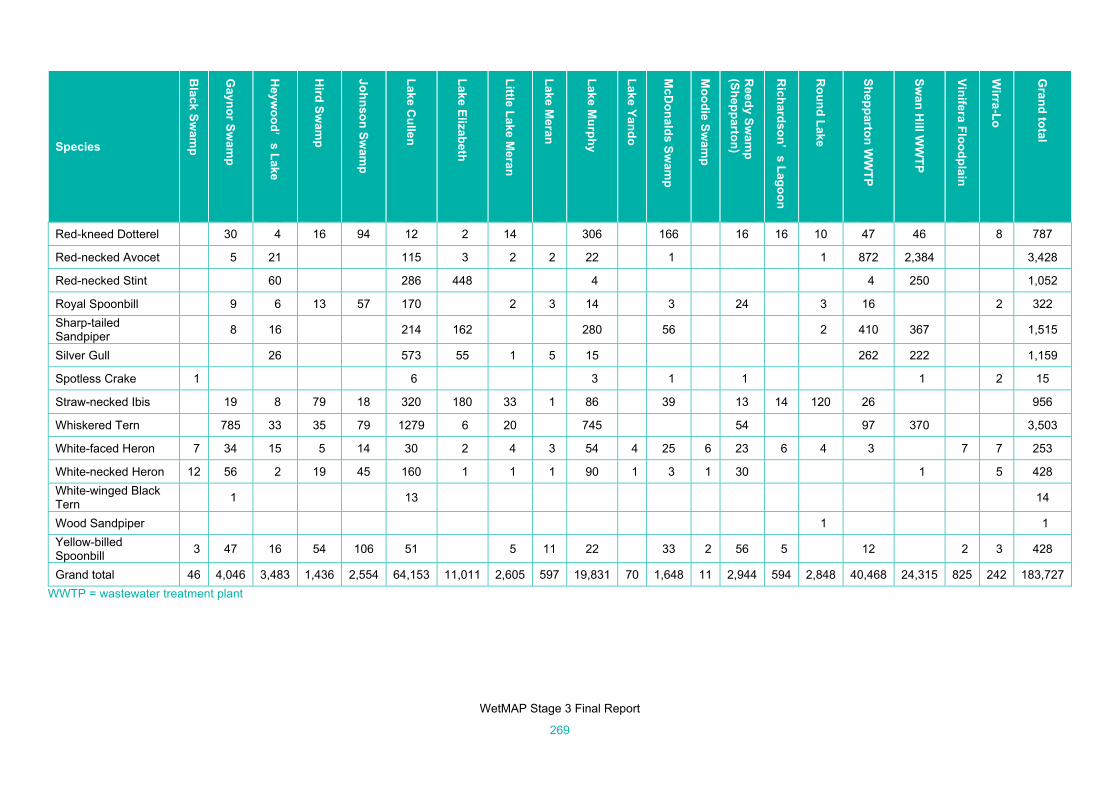
WetMAP Stage 3 Final Report
269
Species
Black S
wam
p
Gayn
or S
wam
p
Heyw
oo
d’
s Lake
Hird
Sw
amp
Joh
nso
n S
wam
p
Lake C
ullen
Lake E
lizabeth
Little L
ake Meran
Lake M
eran
Lake M
urp
hy
Lake Y
and
o
McD
on
alds S
wam
p
Mo
od
ie Sw
amp
Reed
y Sw
amp
(S
hep
parto
n)
Rich
ardso
n’
s Lag
oo
n
Ro
un
d L
ake
Sh
epp
arton
WW
TP
Sw
an H
ill WW
TP
Vin
ifera Flo
od
plain
Wirra-L
o
Gran
d to
tal
Red-kneed Dotterel 30 4 16 94 12 2 14 306 166 16 16 10 47 46 8 787
Red-necked Avocet 5 21 115 3 2 2 22 1 1 872 2,384 3,428
Red-necked Stint 60 286 448 4 4 250 1,052
Royal Spoonbill 9 6 13 57 170 2 3 14 3 24 3 16 2 322
Sharp-tailed Sandpiper
8 16 214 162 280 56 2 410 367 1,515
Silver Gull 26 573 55 1 5 15 262 222 1,159
Spotless Crake 1 6 3 1 1 1 2 15
Straw-necked Ibis 19 8 79 18 320 180 33 1 86 39 13 14 120 26 956
Whiskered Tern 785 33 35 79 1279 6 20 745 54 97 370 3,503
White-faced Heron 7 34 15 5 14 30 2 4 3 54 4 25 6 23 6 4 3 7 7 253
White-necked Heron 12 56 2 19 45 160 1 1 1 90 1 3 1 30 1 5 428
White-winged Black Tern
1 13 14
Wood Sandpiper 1 1
Yellow-billed Spoonbill
3 47 16 54 106 51 5 11 22 33 2 56 5 12 2 3 428
Grand total 46 4,046 3,483 1,436 2,554 64,153 11,011 2,605 597 19,831 70 1,648 11 2,944 594 2,848 40,468 24,315 825 242 183,727
WWTP = wastewater treatment plant
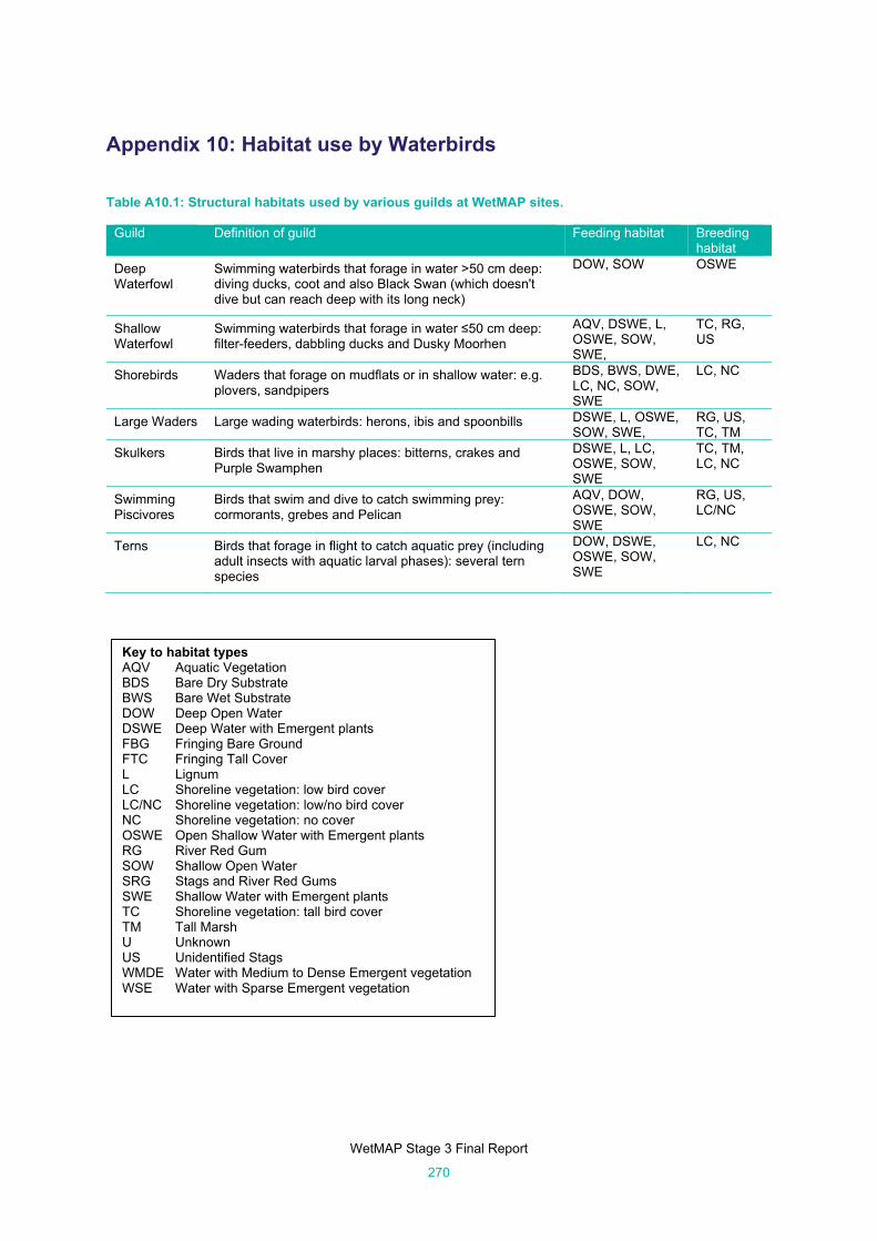
WetMAP Stage 3 Final Report
270
Appendix 10: Habitat use by Waterbirds Table A10.1: Structural habitats used by various guilds at WetMAP sites.
Guild Definition of guild Feeding habitat Breeding habitat
Deep Waterfowl
Swimming waterbirds that forage in water >50 cm deep: diving ducks, coot and also Black Swan (which doesn't dive but can reach deep with its long neck)
DOW, SOW OSWE
Shallow Waterfowl
Swimming waterbirds that forage in water ≤50 cm deep: filter-feeders, dabbling ducks and Dusky Moorhen
AQV, DSWE, L, OSWE, SOW, SWE,
TC, RG, US
Shorebirds Waders that forage on mudflats or in shallow water: e.g. plovers, sandpipers
BDS, BWS, DWE, LC, NC, SOW, SWE
LC, NC
Large Waders Large wading waterbirds: herons, ibis and spoonbills DSWE, L, OSWE, SOW, SWE,
RG, US, TC, TM
Skulkers Birds that live in marshy places: bitterns, crakes and Purple Swamphen
DSWE, L, LC, OSWE, SOW, SWE
TC, TM, LC, NC
Swimming Piscivores
Birds that swim and dive to catch swimming prey: cormorants, grebes and Pelican
AQV, DOW, OSWE, SOW, SWE
RG, US, LC/NC
Terns Birds that forage in flight to catch aquatic prey (including adult insects with aquatic larval phases): several tern species
DOW, DSWE, OSWE, SOW, SWE
LC, NC
Key to habitat types AQV Aquatic Vegetation BDS Bare Dry Substrate BWS Bare Wet Substrate DOW Deep Open Water DSWE Deep Water with Emergent plants FBG Fringing Bare Ground FTC Fringing Tall Cover L Lignum LC Shoreline vegetation: low bird cover LC/NC Shoreline vegetation: low/no bird cover NC Shoreline vegetation: no cover OSWE Open Shallow Water with Emergent plants RG River Red Gum SOW Shallow Open Water SRG Stags and River Red Gums SWE Shallow Water with Emergent plants TC Shoreline vegetation: tall bird cover TM Tall Marsh U Unknown US Unidentified Stags WMDE Water with Medium to Dense Emergent vegetation WSE Water with Sparse Emergent vegetation

WetMAP Stage 3 Final Report
271
Table A10.2: Model selection results exploring the relationship between total bird numbers and hydrological predictors and wetland area.
Variable AICc Delta Weight
Wet proportion (30 days) + Area 3096.9 0.00 0.92
Wet proportion (30 days) 3101.8 4.92 0.08
Wet proportion (90 days) 3110.1 13.19 0.00
Wet proportion 3115.4 18.45 0.00
Wet proportion (30 days) + Area * Season 3126.6 29.67 0.00
Time since wetland was dry 3132.6 35.69 0.00
Wet proportion (180 days) 3134.8 37.94 0.00
Wet proportion (360 days) 3156.5 59.55 0.00
Area 3159.7 62.83 0.00
Null 3163.5 66.64 0.00
Table A10.3: Model selection results exploring the relationship between total waterbird numbers and hydrological predictors and wetland area.
Variable AICc Delta Weight
Wet proportion (90 days) 2921.8 0.00 0.66
Wet proportion (30 days) + Area 2924.4 2.58 0.18
Wet proportion (30 days) 2924.7 2.87 0.16
Wet proportion 2961.8 39.98 0.00
Time since wetland was dry 2988.6 66.77 0.00
Wet proportion (180 days) 2995.0 73.24 0.00
Wet proportion (360 days) 3049.2 127.44 0.00
Area 3063.9 142.07 0.00
Null 3064.6 142.85 0.00
Table A10.4: Model selection results exploring the relationship between Black-winged Stilts and hydrological predictors and wetland area.
Variable AICc Delta Weight
Wet proportion (30 days) 1244.7 0.00 0.37
Wet proportion (30 days) + Area 1245.4 0.77 0.25
Time since wetland was dry 1246.3 1.64 0.16
Wet proportion (90 days) 1246.5 1.82 0.15
Area 1250.2 5.49 0.02
Wet proportion (180 days) 1250.3 5.61 0.02
Wet proportion (360 days) 1250.8 6.16 0.02
Wet proportion 1253.1 8.43 0.01
Null 1264.0 19.31 0.00

WetMAP Stage 3 Final Report
272
Table A10.5: Model selection results exploring the relationship between Black Swan and hydrological predictors and wetland area.
Variable AICc Delta Weight
Wet proportion (90 days) + Area 1445.4 0.00 0.47
Wet proportion (90 days) 1445.6 0.17 0.44
Wet proportion (30 days) 1448.7 3.27 0.09
Wet proportion 1464.0 18.62 0.00
Wet proportion (180 days) 1464.4 18.98 0.00
Wet proportion (360 days) 1467.2 21.74 0.00
Time since wetland was dry 1474.8 29.39 0.00
Area 1476.1 30.70 0.00
Null 1500.4 54.97 0.00
Table A10.6: Model selection results exploring the relationship between Hoary-headed Grebe and hydrological predictors and wetland area.
Variable AICc Delta Weight
Wet proportion 1351.3 0.00 0.55
Wet proportion + Area 1352.7 1.41 0.27
Wet proportion (30 days) 1353.6 2.31 0.17
Wet proportion (90 days) 1369.0 17.66 0.00
Wet proportion (180 days) 1373.8 22.49 0.00
Time since wetland was dry 1387.1 35.76 0.00
Wet proportion (360 days) 1387.8 36.49 0.00
Area 1394.7 43.40 0.00
Null 1403.2 51.92 0.00
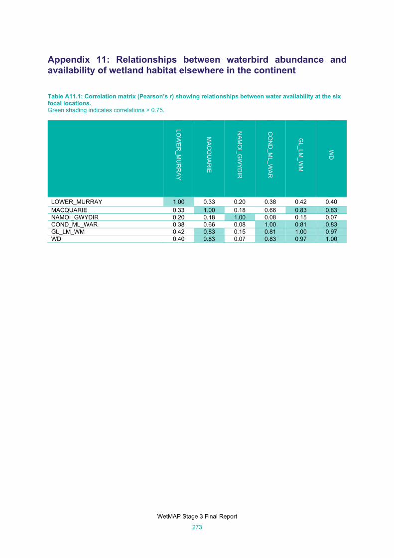
WetMAP Stage 3 Final Report
273
Appendix 11: Relationships between waterbird abundance and availability of wetland habitat elsewhere in the continent Table A11.1: Correlation matrix (Pearson’s r) showing relationships between water availability at the six focal locations. Green shading indicates correlations > 0.75.
LOW
ER
_MU
RR
AY
MA
CQ
UA
RIE
NA
MO
I_GW
YD
IR
CO
ND
_ML
_WA
R
GL_LM
_WM
WD
LOWER_MURRAY 1.00 0.33 0.20 0.38 0.42 0.40 MACQUARIE 0.33 1.00 0.18 0.66 0.83 0.83 NAMOI_GWYDIR 0.20 0.18 1.00 0.08 0.15 0.07 COND_ML_WAR 0.38 0.66 0.08 1.00 0.81 0.83 GL_LM_WM 0.42 0.83 0.15 0.81 1.00 0.97 WD 0.40 0.83 0.07 0.83 0.97 1.00

WetMAP Stage 3 Final Report
274
Table A11.2: Summary of generalised additive models (GAMs). The p-value for location is given for the smoother for water availability at a particular location (where p < 0.05 indicates a relationship). The p-value for year evaluates any yearly trend. ‘Location’, ‘AICc’ and ‘Delta AIC’ relate to model selection. (Delta AIC provides evidence that a model is a significantly better fit.) NAs in the table for the p (year) column indicate no yearly trend detected. The Lower Murray location had less data, so this location was not included in the model selection process.
Summer Winter
Species Location AICc Delta AIC
Weight p (location) p (year) Location AICc Delta AIC
Weight p (location) p (year)
Pink-eared Duck
GL_LM_WM 201.80 0.00 0.98 <0.01 NA GL_LM_WM 193.6 0.00 0.96 0.02 NA
Null 210.30 8.49 0.01 NA NA Null 200.3 6.74 0.03 NA NA
Namoi_Gwydir 212.50 10.70 0.01 0.46 NA Namoi_Gwydir 203.2 9.59 0.01 0.94 NA
Lower_Murray NA NA NA 0.67 NA Lower_Murray NA NA NA 0.08 NA
Freckled Duck GL_LM_WM 70.80 0.00 0.78 0.06 NA Null 76.1 0 0.39 NA NA
Null 73.90 3.09 0.17 NA NA GL_LM_WM 76.5 0.39 0.32 0.23 NA
Namoi_Gwydir 76.20 5.35 0.05 0.56 NA Namoi_Gwydir 76.7 0.59 0.2 0.16 NA
Lower_Murray NA NA NA <0.01 NA Lower_Murray NA NA NA 0.11 NA
Eurasian Coot
GL_LM_WM 367.50 0.00 0.89 0.07 0.04 GL_LM_WM 329.50 0.00 0.76 0.10 0.06
Namoi_Gwydir 372.50 4.99 0.07 0.90 <0.01 Namoi_Gwydir 331.90 2.40 0.23 0.94 <0.01
Null 373.80 6.30 0.04 NA NA Null 338.00 8.52 0.01 NA NA
Lower_Murray NA NA NA 0.35 <0.01 Lower_Murray NA NA NA 0.67 <0.01
Grey Teal GL_LM_WM 344.10 0.00 0.83 0.04 <0.01 Namoi_Gwydir 375.40 0.00 0.59 0.20 0.04
Null 347.60 3.57 0.14 NA NA GL_LM_WM 377.20 1.80 0.24 0.81 0.05
Namoi_Gwydir 351.00 6.91 0.03 0.57 <0.01 Null 377.80 2.39 0.18 NA NA
Lower_Murray NA NA NA 0.80 <0.01 Lower_Murray NA NA NA 0.46 0.04
Chestnut Teal GL_LM_WM 339.90 0.00 0.62 0.12 NA GL_LM_WM 318.10 0.00 0.74 0.06 NA
Null 341.30 1.42 0.30 NA NA Namoi_Gwydir 321.40 3.23 0.15 0.12 NA
Namoi_Gwydir 344.10 4.21 0.08 0.03 NA Null 321.90 3.76 0.11 NA NA
Lower_Murray NA NA NA 0.07 NA Lower_Murray NA NA NA 0.12 NA

WetMAP Stage 3 Final Report
275
Summer Winter
Species Location AICc Delta AIC
Weight p (location) p (year) Location AICc Delta AIC
Weight p (location) p (year)
Hoary-headed Grebe
GL_LM_WM 382.00 0.00 0.82 0.03 0.29 GL_LM_WM 352.70 0.00 0.70 0.06 NA
Null 385.30 3.36 0.15 NA NA Null 355.20 2.50 0.20 NA NA
Namoi_Gwydir 388.70 6.76 0.03 0.82 0.20 Namoi_Gwydir 356.70 4.02 0.10 0.37 NA
Lower_Murray NA NA NA 0.61 <0.01 Lower_Murray NA NA NA 0.51 NA
Australian Shelduck
GL_LM_WM 377.7 0 0.87 0.06 <0.01 GL_LM_WM 210.6 0.00 0.59 0.12 NA
Namoi_Gwydir 381.5 3.79 0.13 0.64 <0.01 Null 211.8 1.21 0.32 NA NA
Null 422.6 44.89 0 NA NA Namoi_Gwydir 214.2 3.73 0.09 0.59 NA
Lower_Murray NA NA NA 0.78 <0.01 Lower_Murray NA NA NA 0.23 NA
Blue-billed Duck
GL_LM_WM 169.20 0.00 1.00 0.02 0.17 GL_LM_WM 348.9 0.00 0.62 0.10 NA
Null 181.20 11.96 0.00 NA NA Null 350.3 1.46 0.30 NA NA
Namoi_Gwydir 181.70 12.50 0.00 0.56 0.06 Namoi_Gwydir 353.0 4.16 0.08 0.72 NA
Lower_Murray NA NA NA 0.64 0.14 Lower_Murray NA NA NA 0.03 NA
Sharp-tailed Sandpiper
GL_LM_WM 92.00 0.00 0.63 0.11 <0.01 GL_LM_WM 91.90 0.00 0.46 0.10 NA
Namoi_Gwydir 93.30 1.26 0.34 0.15 <0.01 Null 92.20 0.31 0.39 NA NA
Null 98.20 6.17 0.03 NA NA Namoi_Gwydir 94.10 2.17 0.15 0.35 NA
Lower_Murray NA NA NA 0.22 0.03 Lower_Murray NA NA NA 0.12 NA
Australasian Shoveler
GL_LM_WM 341.40 0.00 0.93 <0.01 <0.01 Namoi_Gwydir 333.8 0.00 0.48 0.26 <0.01
Namoi_Gwydir 347.50 6.06 0.05 0.14 <0.01 Null 334.3 0.55 0.36 NA NA
Null 349.00 7.59 0.02 NA NA GL_LM_WM 336.0 2.20 0.16 0.96 <0.01
Lower_Murray NA NA NA 0.55 <0.01 Lower_Murray NA NA NA 0.56 <0.01
Whiskered Tern
GL_LM_WM 171.3 0.00 0.98 <0.01 <0.01 Null 121.5 0.00 0.75 NA NA
Null 179.0 7.66 0.02 NA NA GL_LM_WM 124.2 2.72 0.19 0.75 NA
Namoi_Gwydir 182.2 10.82 0.00 0.78 0.04 Namoi_Gwydir 126.5 5.00 0.06 0.30 NA
Lower_Murray NA NA NA 0.76 NA Lower_Murray NA NA NA 0.56 NA

WetMAP Stage 3 Final Report
276
Appendix 12: Catch of all fish species caught in wetlands using fine-mesh fyke nets and seine hauls Table A12.1: Catch of all fish species caught in wetlands using fine-mesh fyke nets and seine hauls during surveys from October 2018 to February 2020. Invasive species are denoted by an asterisk (*); non-sampled times are denoted by an en dash (–).
Wetland
2018 2019 2020
16 Oct
29 Oct
11 Feb
29 Apr
19 Aug
14 Oct
11 Nov
10 Feb
Catfish Lagoon
Australian Smelt (Retropinna semoni) 1 51 12 2 330 241 437 15
Carp Gudgeon (Hypseleotris spp.) 163 7 2206 721 71 230 2820 1907
Un-specked Hardyhead (Craterocephalus fulvus) 0 0 66 0 0 0 7 0
Flat-headed Gudgeon (Philypnodon grandiceps) 0 0 0 0 0 0 4 0
Golden Perch (Macquaria ambigua) 0 1 0 0 0 0 0 0
Murray Cod (Maccullochella peelii) 0 1 0 0 0 0 0 0
Goldfish (Carassius auratus*) 0 2 0 0 0 0 0 0
Carp (Cyprinus carpio*) 7 37 0 0 0 0 1842 0
Eastern Gambusia (Gambusia holbrooki*) 8 18 622 744 5 6 180 647
Oriental Weatherloach (Misgurnus anguilicaudatus*)
1 0 0 0 0 0 0 0
Total catch 180 117 2906 1467 406 477 5290 2569
Ducksfoot Lagoon
Australian Smelt (Retropinna semoni) 90 51 264 6 2 21 81 541
Carp Gudgeon (Hypseleotris spp.) 4805 12883 2743 1244 56 2074 477 6426
Un-specked Hardyhead (Craterocephalus fulvus) 133 99 148 45 12 10 22 900
Murray River Rainbowfish (Melanotaenia fluviatilis)
8 5 74 6 2 10 14 313
Bony Bream (Nematalosa erebi) 0 0 2 1 0 0 0 5
Goldfish (Carassius auratus*) 0 0 1 0 0 0 0 0
Eastern Gambusia (Gambusia holbrooki*) 19 47 2318 75 21 24 18 529
Carp (Cyprinus carpio*) 0 0 208 0 0 1346 2848 0
Oriental Weatherloach (Misgurnus anguilicaudatus*)
0 1 0 0 0 11 132 5
Total catch 5055 13086 5758 1377 93 3496 3592 8719
Margooya Lagoon
Australian Smelt (Retropinna semoni) 3110 492 1 0 41 66 838 0
Carp Gudgeon (Hypseleotris spp.) 29437 33501 10980 3048 1340 3545 7805 38128
Un-specked Hardyhead (Craterocephalu fulvus) 0 0 0 0 1 0 2 876
Flat-headed Gudgeon (Philypnodon grandiceps) 0 0 7 0 1 0 8 227
Murray River Rainbowfish (Melanotaenia fluviatilis)
0 0 3 0 0 0 0 26
Goldfish (Carassius auratus*) 21 2715 0 0 0 0 0 0
Eastern Gambusia (Gambusia holbrooki*) 0 0 1663 3594 377 9 13 38307
Carp (Cyprinus carpio*) 84 0 89 6 0 57 116 0
Oriental Weatherloach (Misgurnus anguilicaudatus*)
3 16 28 115 0 45 9 14
Total catch 32655 36724 12771 6763 1760 3722 8791 77578

WetMAP Stage 3 Final Report
277
Table A12.1 continued
Wetland 2019 2020
18 Feb 8 Apr 5 Aug 4 Nov 25 Nov 24 Feb
Bunyip Swamp
Carp Gudgeon (Hypseleotris spp.) 1784 3013 1115 738 650 –
Goldfish (Carassius auratus*) 0 3 0 0 0 –
Eastern Gambusia (Gambusia holbrooki*) 0 2 0 0 1 –
Carp (Cyprinus carpio*) 180 98 7 0 0 –
Oriental Weatherloach (Misgurnus anguilicaudatus*) 0 2 1 4 10 –
Total catch 1964 3118 1123 742 661 –
Cucumber Gully
Australian Smelt (Retropinna semoni) 14 39 40 54 44 0
Carp Gudgeon (Hypseleotris spp.) 5856 5559 1136 4777 5935 0
Goldfish (Carassius auratus*) 0 6 0 0 13 0
Eastern Gambusia (Gambusia holbrooki*) 1744 2174 51 1 15 0
Carp (Cyprinus carpio*) 55 315 5 0 0 0
Oriental Weatherloach (Misgurnus anguilicaudatus*) 0 5 0 27 0 5
Total catch 7669 8098 1232 4859 6007 5
Hut Lake
Australian Smelt (Retropinna semoni) 13 9 395 507 1006 0
Carp Gudgeon (Hypseleotris spp.) 1082 1552 310 319 405 2412
Murray River Rainbowfish (Melanotaenia fluviatilis) 22 2 0 0 0 0
Un-specked Hardyhead (Craterocephalus fulvus) 2 9 0 0 0 0
Goldfish (Carassius auratus*) 15 5 15 2 1278 6
Eastern Gambusia (Gambusia holbrooki*) 4106 266 2 192 510 222
Carp (Cyprinus carpio*) 0 1 1 7073 1405 21
Oriental Weatherloach (Misgurnus anguilicaudatus*) 48 14 40 48 11 352
Total catch 5288 1858 763 8141 4615 3013
Tarma Lagoon
Australian Smelt (Retropinna semoni) 103 29 24 1296 1302 606
Carp Gudgeon (Hypseleotris spp.) 900 702 78 5225 4847 2112
Obscure Galaxias (Galaxias oliros) 0 0 0 1 0 0
Goldfish (Carassius auratus*) 19 15 14 0 28 2
Eastern Gambusia (Gambusia holbrooki*) 204 47 1 8 76 909
Carp (Cyprinus carpio*) 343 144 6 5720 1404 1
Oriental Weatherloach (Misgurnus anguilicaudatus*) 20 116 6 3 6 11
Total catch 1589 1053 129 12253 7663 3641

WetMAP Stage 3 Final Report
278
Appendix 13: The percentage of total wetland area inundated at three wetlands, demonstrating the three watering types designated in this study
Figure A13.1: The percentage of total wetland area inundated at three wetlands, demonstrating the three watering types designated in this study.
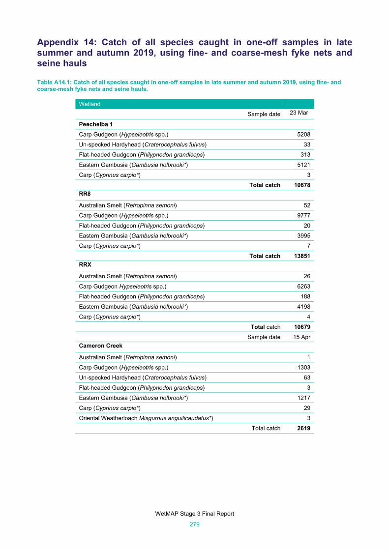
WetMAP Stage 3 Final Report
279
Appendix 14: Catch of all species caught in one-off samples in late summer and autumn 2019, using fine- and coarse-mesh fyke nets and seine hauls Table A14.1: Catch of all species caught in one-off samples in late summer and autumn 2019, using fine- and coarse-mesh fyke nets and seine hauls.
Wetland
Sample date 23 Mar
Peechelba 1
Carp Gudgeon (Hypseleotris spp.) 5208
Un-specked Hardyhead (Craterocephalus fulvus) 33
Flat-headed Gudgeon (Philypnodon grandiceps) 313
Eastern Gambusia (Gambusia holbrooki*) 5121
Carp (Cyprinus carpio*) 3
Total catch 10678
RR8
Australian Smelt (Retropinna semoni) 52
Carp Gudgeon (Hypseleotris spp.) 9777
Flat-headed Gudgeon (Philypnodon grandiceps) 20
Eastern Gambusia (Gambusia holbrooki*) 3995
Carp (Cyprinus carpio*) 7
Total catch 13851
RRX
Australian Smelt (Retropinna semoni) 26
Carp Gudgeon Hypseleotris spp.) 6263
Flat-headed Gudgeon (Philypnodon grandiceps) 188
Eastern Gambusia (Gambusia holbrooki*) 4198
Carp (Cyprinus carpio*) 4
Total catch 10679
Sample date 15 Apr
Cameron Creek
Australian Smelt (Retropinna semoni) 1
Carp Gudgeon (Hypseleotris spp.) 1303
Un-specked Hardyhead (Craterocephalus fulvus) 63
Flat-headed Gudgeon (Philypnodon grandiceps) 3
Eastern Gambusia (Gambusia holbrooki*) 1217
Carp (Cyprinus carpio*) 29
Oriental Weatherloach Misgurnus anguilicaudatus*) 3
Total catch 2619

WetMAP Stage 3 Final Report
280
Table A14.1 continued
Wetland
Sample date 6 May
Black Swamp
Australian Smelt (Retropinna semoni) 53
Carp Gudgeon (Hypseleotris spp.) 20711
Murray River Rainbowfish (Melanotaenia fluviatilis) 8
Golden Perch (Macquaria ambigua) 2
Goldfish (Carassius auratus*) 1
Eastern Gambusia (Gambusia holbrooki*) 3140
Total catch 23915
Punt Paddock
Australian Smelt (Retropinna semoni) 258
Carp Gudgeon (Hypseleotris spp.) 1435
Un-specked Hardyhead (Craterocephalus fulvus) 20
Murray River Rainbowfish Melanotaenia fluviatilis) 18
Flat-headed Gudgeon (Philypnodon grandiceps) 6
Dwarf Flat-headed Gudgeon (Philypnodon macrostomus) 1
Goldfish (Carassius auratus*) 3
Eastern Gambusia (Gambusia holbrooki*) 67
Carp (Cyprinus carpio*) 2
Oriental Weatherloach (Misgurnus anguilicaudatus*) 2
Total catch 1812
Sharpes Lagoon
Australian Smelt (Retropinna semoni) 351
Carp Gudgeon (Hypseleotris spp.) 7469
Un-specked Hardyhead (Craterocephalus fulvus) 209
Murray River Rainbowfish (Melanotaenia fluviatilis) 6
Flat-headed Gudgeon (Philypnodon grandiceps) 134
Eastern Gambusia (Gambusia holbrooki*) 64
Total catch 8233

WetMAP Stage 3 Final Report
281
Appendix 15: Catch of all species trapped moving in and out of wetlands in double-winged fyke nets. Table A15.1: Catch of all species trapped moving in and out of wetlands in double-winged fyke net at connecting channels and forest channels. Invasive species are denoted by asterisks (*), non-sampled times are denoted by en dashes (–).
Channel 2018 2019
Oct Nov Feb Aug Sep Oct Nov
In Out In Out In Out In Out In Out In Out In Out
Ducksfoot Lagoon connecting channel Australian Smelt Retropinna semoni 2 26 6 3160 – – – – 12 65 9 4205 0 930 Carp Gudgeon Hypseleotris spp. 94 45 1136 10574 – – – – 171 63 395 205 304 34 Bony Bream Nematalosa erebi 2 3 3 8 – – – – 8 0 9 7 2 11 Un-specked Hardyhead Craterocephalus fulvus 0 1 0 1 – – – – 0 0 0 0 7 0 Goldfish Carassius auratus 0 0 0 0 – – – – 0 0 0 0 15 39 Murray River Rainbowfish Melanotaenia fluviatilis 0 0 0 0 – – – – 0 0 1 0 0 1 Golden Perch Macquaria ambugua 0 1 0 0 – – – – 0 2 2 0 0 0 Carp Cyprinus carpio* 0 0 0 0 – – – – 0 0 9 2 72 167 Gambusia Gambusia holbrooki* 0 0 0 0 – – – – 1 2 0 0 0 0 Oriental Weatherloach Misgurnus anguilicaudatus* 0 0 0 0 – – – – 0 3 1 0 0 2
Total catch 98 76 1145 13743 – – – – 192 135 426 4419 400 1184 Margooya Lagoon connecting channel Australian Smelt Retropinna semoni 90 35 13 8751 0 0 50 50 22 3 414 26452 166 109 Carp Gudgeon Hypseleotris spp. 1400 1127 365 664 115 156219 61 39 619 2963 13520 9878 5201 6935 Bony Bream Nematalosa erebi 0 0 14 0 0 0 0 0 0 0 9 47 5 0 Un-specked Hardyhead Craterocephalus fulvus 0 1 0 0 0 0 0 0 0 0 371 31 3 0 Murray River Rainbowfish Melanotaenia fluviatilis 0 0 0 0 0 0 0 0 0 0 6 0 1 0 Flat-headed Gudgeon Philypnodon grandiceps 0 0 0 0 0 0 0 0 0 0 6 0 0 7 Obscure Galaxias Galaxias oliros 0 0 0 0 0 0 0 0 0 0 1 28 0 0 Freshwater Catfish Tandanus tandanus 0 0 0 0 0 0 0 0 0 0 1 0 0 0 Murray Cod Maccullochella peelii 0 0 0 0 0 0 0 0 0 0 0 0 1 0 Goldfish Carassius auratus* 3 3 0 0 3 0 0 0 1 0 21 27 160 169 Carp Cyprinus carpio* 0 0 92 1413 9 2 0 0 0 0 3 18 167 220 Gambusia Gambusia holbrooki* 0 0 0 0 1 44 9 0 14 0 11 8 19 23 Oriental Weatherloach Misgurnus anguilicaudatus* 0 0 0 0 0 0 5 0 8 10 73 150 43 124
Total catch 1493 1166 484 10828 128 156265 125 89 664 2976 14436 36639 5766 7587

WetMAP Stage 3 Final Report
282
Table A15.1 continued
Channel Sep 2019
In Out
Barmah Large regulator (forest channel)
Australian Smelt (Retropinna semoni) 57 105
Carp Gudgeon (Hypseleotris spp.) 7 0
Gambusia (Gambusia holbrooki*) 1 0
Goldfish (Carassus auratus*) 0 1
Total catch 65 106
Barmah Small Regulator (forest channel)
Australian Smelt (Retropinna semoni) 58 342
Carp Gudgeon (Hypseleotris spp.) 26 0
Gambusia (Gambusia holbrooki*) 0 1
Oriental Weatherloach (Misgurnus anguilicaudatus*) 1 0
Total catch 85 343
Hut Lake (forest channel)
Australian Smelt (Retropinna semoni) 351 4
Carp Gudgeon (Hypseleotris spp.) 0 7
Gambusia (Gambusia holbrooki*) 0 1
Oriental Weatherloach (Misgurnus anguilicaudatus*) 0 8
Total catch 351 20
Green Swamp (forest channel)
Australian Smelt (Retropinna semoni) 7 84
Carp Gudgeon (Hypseleotris spp.) 9004 6679
Murray River Rainbowfish (Melanotaenia fluviatilis) 3 2
Gambusia (Gambusia holbrooki*) 68 18
Goldfish (Carassus auratus*) 1 0
Carp (Cyprinus carpio*) 6 0
Total catch 9089 6783
Shillingslaw Regulator (forest channel)
Australian Smelt (Retropinna semoni) 204 85
Carp Gudgeon (Hypseleotris spp.) 8 7
Gambusia (Gambusia holbrooki*) 0 1
Total catch 212 93
Yarran Regulator (forest channel)
Australian Smelt (Retropinna semoni) 163 1042
Carp Gudgeon (Hypseleotris spp.) 33 69
Un-specked Hardyhead (Craterocephalus fulvus) 1 0
Murray Cod (Maccullochella peelii) 1 0
Total catch 198 1111

WetMAP Stage 3 Final Report
283
Appendix 16: Catch through time of Carp Gudgeon (Hypseleotris spp.) at wetlands in Barmah Forest (GBCMA)
Figure A16.1: Catch through time of Carp Gudgeon (Hypseleotris spp.) at wetlands in Barmah Forest (GBCMA). Large circles represent mean catch per fyke net for each trip, and small circles represent the catch for each net.

WetMAP Stage 3 Final Report
284
Appendix 17: Catch through time of Carp Gudgeon (Hypseleotris spp.) at wetlands in the Mallee Region
Figure A17.1: Catch through time of Carp Gudgeon (Hypseleotris spp.) at wetlands in the Mallee Region. Large circles represent mean catch per fyke net for each trip, and small circles represent the catch for each net.

WetMAP Stage 3 Final Report
285
Appendix 18: Catch through time of Australian Smelt (Retropinna semoni) at wetlands in Barmah Forest (GBCMA)
Figure A18.1: Catch through time of Australian Smelt (Retropinna semoni) at wetlands in Barmah Forest (GBCMA). Large circles represent mean catch per fyke net for each trip, and small circles represent the catch for each net.

WetMAP Stage 3 Final Report
286
Appendix 19: Catch through time of Australian Smelt (Retropinna semoni) at wetlands in the Mallee Region
Figure A19.1: Catch through time of Australian Smelt (Retropinna semoni) at wetlands in the Mallee Region. Large circles represent mean catch per fyke net for each trip, and small circles represent the catch for each net.

WetMAP Stage 3 Final Report
287
Appendix 20: Frog citizen science – communication tools and preliminary evaluation
Engagement outputs Flyer, poster
A flyer (on Frogscalling.org) (August 2019) and a poster were produced (on the ARI website) (September 2019) and distributed to NCCMA and GBCMA. Some were distributed by GBCMA at the Shepparton River Festival (September 2019), and more were provided to participants at the bird citizen science field day.
Websites The frogscalling.org website was created as the primary conduit for project information and progress
and was launched in August 2019.
The Victorians Volunteering for Nature page included a project highlight for National Volunteer Week (May 2020).
The project is highlighted as an example of how Protecting Victoria’s Environment – Biodiversity 2037 is being implemented.
DELWP Land for Wildlife newsletter included a project highlight (December 2019).
The ARI website also included The Frogs Are Calling You page, launched in July 2019.
Via the ARI subscriptions page, access to three online products:
o the WetMAP frog citizen science project
o ARI eNews (audience >1500 people); the project was highlighted in September 2019
o ARI Applied Aquatic Ecology Quarterly Update (audience >1300 people); the project was highlighted in January 2020.
The audiences for these online products incorporate most WetMAP citizen science target audiences and represent a diverse and comprehensive mix of commonwealth, state and local government staff, university scientists and students, interest groups, NGOs, consultants and the general public. Some subscribers then onshare content via other websites and e-newsletters.
Content produced by other organisations (including websites and e-newsletters), for example:
VEWH website – Jumping to get outdoors (https://vewh.vic.gov.au/news-and-publications/ stories/jumping-to-get-outdoors-take-a-leap-and-become-a-frog-citizen-scientist) (November 2019); VEWH approached the project lead with a draft newsletter article and request for input. VEWH has since requested further material for their 2019–2020 publication ‘Reflections’.
o CMAs – the NCCMA Landcare and Waterwatch news – North Central CMA Chat (north_central_chat-_november_2019.pdf) (November 2019)
o Victorian Landcare and Catchment Management Magazine, Summer 2020 Issue 77 – Citizen scientists record frog calls for wetland management (https://www.landcarevic.org.au/landcare-magazine/summer-2020/citizen-scientists-record-frog-calls-for-wetland-management/) (January 2020)
Frog ID newsletter - The Frogs Are Calling You: monitoring the impacts of environmental water in northern and western Victoria (April 2020)

WetMAP Stage 3 Final Report
288
o Remember the Wild – How citizens are changing science and how to get involved (https://www.rememberthewild.org.au/how-citizens-are-changing-science-and-how-to-get-involved/) (March 2020)
o Added to Australian Citizen Science finder (https://biocollect.ala.org.au/acsa/project/index/d966bf88-07d3-4775-80a4-c56ad2b81b4d) (January 2020)
Localising Leanganook Newsletter – Citizen Science Frog Project (https://leanganook.org/november-2019-newsletter/) (November 2019)
Videos Videos provide a simple tool to engage audiences and promote the project.
DELWP videos have been discussed and will likely be filmed on future field days.
CMAs – Mallee CMA Frogs of the Mallee is due for imminent release and mentions our project.
Internal social media DELWP has several avenues for promoting the project with internal staff:
DELWP Yammer – provides an efficient way to promote work and share highlights internally within DELWP, with a potential audience of >4500. Tagging participating staff, senior DELWP managers and funders can ensure these Yammers are noticed, and they are sometimes identified by DELWP Corporate Comms staff as having good content for external media.
o WetMAP-related posts were produced: October 2019, highlighting project; March 2020, re field day. Readership of these posts usually ranges in the mid-hundreds.
Ada newsroom posts offer a useful visibility opportunity to DELWP staff, and content is sometimes identified by DELWP Corporate Comms staff as having good content for external media.
o Frog friends – celebrating Citizen Science Month (May 2020)
Fortnightly internal newsletters are produced for Water and Catchments – ‘The Spill’ and Biodiversity ‘Yarn’ – which have also incorporated WetMAP highlights.
o DELWP Biodiversity Yarn included ‘CS Frog’ (August 2019).
External social media
The EWRO Yammer network – project highlight (October 2019); WetMAP bird citizen science field day, including frog project (March 2020)
DELWP Facebook – Loddon Mallee and Hume
Can you hear the frogs calling you? (October 2019)
Media releases and other media stories Media releases are an effective way for stories to be subsequently picked up by a range of local newspapers, as well as radio and television.
DELWP media release: National Science Week 2019 (https://www.wildlife.vic.gov.au/media-releases/science-week-2019-celebrating-citizen-science) (August 2019)
Frogscalling.org media release (Jan 2020). This was then picked up by Sunraysia Daily, Riverine Herald, Seymour Telegraph and Shepparton News.
Radio and podcasts Projects for Wildlife podcast (March 2020)
ABC Goulburn Murray Radio (January 2020)

WetMAP Stage 3 Final Report
289
Preliminary evaluation To date, the data obtained from citizen scientists are relatively few, and collected from sites that are not WetMAP focal wetlands. These data have therefore not yet been included in the WetMAP frog theme analysis, but this may be possible in the future, especially as more citizen scientists are recruited closer to target sites. Future communications will also encourage citizen scientists to record at WetMAP target sites. Despite not having any data collected from target sites, FrogID provided the project with 415 records from within the requested local government areas, suggesting that there are active citizen scientists with potential to collect data at focus sites.
In March 2020, when various movement restrictions were enforced throughout Victoria, engagement messages focused on encouraging citizen scientists to collect data within a short distance of their homes and even on their own properties. Although the onset of COVID-19 restrictions didn’t initially seem to reduce interest in the project, sign-ups by citizen scientists slowed significantly through the winter of 2020 – perhaps in response to the weather as well as public health guidelines. Promotion of the program was relaxed during the second COVID-19 lockdown, with the specific purpose of further promoting the project and specific WetMAP sites in the spring, when the public may be more able to explore the state and the weather improves.
Questionnaires We produced two questionnaires to assess participation and learning by participants:
1. a sign-up questionnaire to assess motivations and recruitment
2. an audience questionnaire for both citizen scientists and participants not officially signed up, to assess leaning and behavioural change.
The sign-up questionnaire was listed as a step in the sign-up process to encourage citizen scientists to complete it. As of 17 July 2020, 31 citizen scientists were signed up for The Frogs Are Calling You and had completed the questionnaire. None of the survey questions was a required field, which was deliberate to reduce pressure on participants. Most questions were answered, with the exception of the last (What actions did you undertake for nature prior to hearing about the WetMAP citizen science frog project?), which was more involved than previous questions, requiring more reading and/or thought to answer. The question may also have been ignored by people who did not feel they performed any of the listed actions. We have since added a ‘None’ answer option. Twenty-two respondents did not answer the last question.
The audience questionnaire was distributed through the sign-up lists, website subscriptions and social media. Anyone who followed the project in any capacity was invited to complete the survey. The questionnaire is distributed with every newsletter, as well as being available on the website and is regularly completed by participants. Previous respondents are invited to complete it again, but as yet nobody has completed it more than once. Of the audience survey respondents, three are citizen scientists, four read the newsletter and three follow the project on social media. Others had multiple connections with the project or didn’t state their connection.
Recruitment of citizen scientists The main ways that citizen scientists heard about and were inspired to join the project was through the popular press and their schools, with five individuals citing each of those sources. The ABC, local newspapers, Landcare and Land for Wildlife newsletter articles all successfully recruited citizen scientists. It is not immediately clear whether the citizen scientists who heard about the project through ‘school’ are children or teachers.
Four people heard about the project through word of mouth, three stated that they heard about the project from a CMA. Other sources of recruitment were Frogs Victoria, WaterWatch, a university lecture, FrogID, an ARI newsletter, internal DELWP communications, internet searches and social media.
The main motivation for participating in the project was cited as ‘I want to make a difference in conservation’ (eight respondents). Six respondents said they were primarily motivated because they love frogs, and five said they wanted to learn more about frogs and wetlands as a primary reason for signing up. Many others referred to the education and entertainment of their children or grandchildren as being strong motivating factors.
Eighteen participants had participated in citizen science before, and four of those said that their previous experience with citizen science was their primary motivation for joining The Frogs Are Calling You. The citizen science projects that they had previously been involved in were FrogID, Victorian Biodiversity Atlas, Questagame, Aussie Backyard Bird Count and other BirdLife surveys. Three of the four had previous experience with FrogID. FrogID was the most represented citizen science project that the participants had done before (four participants).

WetMAP Stage 3 Final Report
290
Participant understanding There were 11 respondents to the audience questionnaire, which is probably not a large enough sample to draw any significant conclusions about impact yet. However, 10 respondents said that they learnt something about frogs from the project, nine said they learnt something about ecology and/or biodiversity, eight learnt something about environmental water and eight said they learned something about WetMAP by participating in The Frogs Are Calling You in some capacity.
Seven citizen scientists had not heard of environmental water when they signed up, but only five said that they didn’t recognise the concept of storage and release of water for environmental reasons. Unsurprisingly, these same five stated that they had never had a conversation about environmental water. Most people at least recognised environmental water, even if they hadn’t been able or inclined to articulate it before sign-up.
Twenty-two participants had not heard of WetMAP when they signed up. The longer people have participated in The Frogs Are Calling You, the more likely they were to report greater knowledge of frogs (Table A20.1), ecology and/or biodiversity (Table A20.2), environmental water (Table A20.3) and WetMAP (Table A20.4).
Discussion of issues One of our aims was to increase awareness, support and advocacy for frogs, biodiversity and environmental water. Despite the small number of respondents to the audience questionnaire, preliminary results suggest that participants may be more likely to discuss these issues the longer they have been involved in the project (Table A20.5).

WetMAP Stage 3 Final Report
291
Table A20.1: Self-reported knowledge of frogs in citizen scientists and audience questionnaire respondents in relation to the length of their involvement.
Prior to
involvement
(n = 10)
A few days to a few
weeks
(n = 3)
A few weeks to a
few months
(n = 3)
More than a few
months
(n = 4)
Minimal 30% 0% 33% 0%
Moderate 50% 100% 33% 33%
Pretty good 0% 0% 0% 33%
Amazing 20% 0% 33% 33% Table A20.2: Self-reported knowledge about ecology and/or biodiversity in citizen scientists and audience questionnaire respondents in relation to the length of their involvement.
Prior to
involvement
(n = 11)
A few days to a few
weeks
(n = 4)
A few weeks to a
few months
(n = 3)
More than a few
months
(n = 4)
Minimal 27% 25% 33% 0%
Moderate 55% 50% 33% 50%
Pretty good 9% 25% 33% 25%
Amazing 9% 0% 0% 25% Table A20.3: Self-reported knowledge about environmental water in audience questionnaire respondents in relation to the length of their involvement.
Prior to
involvement
(n = 11)
A few days to a few
weeks
(n = 4)
A few weeks to a
few months
(n = 3)
More than a few
months
(n = 4)
Minimal 27% 0% 67% 0%
Moderate 55% 75% 33% 50%
Pretty good 9% 25% 0% 25%
Amazing 9% 0% 0% 25% Table A20.4: Self-reported knowledge about WetMAP in audience questionnaire respondents in relation to the length of their involvement.
Prior to
involvement
(n = 11)
A few days to a few
weeks
(n = 4)
A few weeks to a
few months
(n = 3)
More than a few
months
(n = 4)
Minimal 100% 25% 67% 25%
Moderate 0% 75% 33% 50%
Pretty good 0% 0% 0% 25%
Amazing 0% 0% 0% 0%

WetMAP Stage 3 Final Report
292
Table A20.5: Reported frequency of discussion of project-related subjects. Discussions about environmental water and frogs are reported from both the sign-up questionnaire and the audience questionnaire. WetMAP and ecology/biodiversity discussions are reported only during the audience questionnaire.
Frequency of
discussion
WetMAP Environmental water Ecology and/or
biodiversity
Frogs
Before
(n = 11)
During
(n = 11)
Before
(n = 41)
During
(n = 11)
Before
(n = 11)
During
(n = 11)
Before
(n = 41)
During
(n = 10)
Never 82% 55% 20% 18% 9% 9% 7% 20%
Less than once a year 9% 9% 15% 9% 36% 27% 5% 0%
About once a year 9% 9% 7% 0% 0% 0% 12% 0%
About once every
6 months
0% 0% 0% 0% 0% 0% 10% 0%
About once every few
months
0% 9% 39% 45% 9% 9% 5% 20%
Once every few weeks
or more
0% 0% 20% 27% 45% 55% 61% 60%
Support for environmental water All but one respondent said that high priority should be given to water entitlements for frogs and other native biota. The one anomalous respondent (who had been following the project on social media for only a few days to a few weeks) answered that medium priority should be given to both. Other suggestions for high priority were agriculture and birds.
Behavioural change In addition to learning about frogs, biodiversity, environmental water and WetMAP, participants have also reported greater participation in a broader range of environmental activities since hearing about The Frogs Are Calling You (Table A20.6). Encouragingly, there was a large increase in the amount of advocacy that participants reported.

WetMAP Stage 3 Final Report
293
Table A20.6: Number of participants reporting environmental activity in relation to the length of involvement with The Frogs Are Calling You; includes data from both sign-up questionnaire and audience questionnaires.
Prior to
involvement
A few days to a few weeks
A few weeks to a few months
More than a few months
Other citizen science projects, scientific
projects or contributions to databases
0 2 1 4
Other conservation projects 3 2 2 2
Waterwise activities (such as limiting showers, growing drought-tolerant plants)
7 2 0 2
Habitat preservation (such as not clearing land, leaving natural vegetation)
5 3 1 2
Habitat restoration/creation (such as building a pond, planting a native garden)
4 3 0 3
Advocating for wetlands or conservation (such as talking with people or organisations, social media posts, signing petitions)
0 2 2 2
None 2 0 0 0

WetMAP Stage 3 Final Report
294
Appendix 21: Bird Citizen Science– communication tools and preliminary evaluation
Principles for engagement It was recognised that a broad approach to outreach was ideal. Opportunities to engage with interested community organisations and agencies to achieve further diversity of participants were actively sought out. Organisations directly contacted in regard to an initial workshop (and program generally) included BirdLife Australia Murray–Goulburn Branch, RiverConnect, Field & Game Australia, adjacent CMAs, Yorta Yorta Nation Aboriginal Corporation, Taungurung Land & Waters Council, academic societies, local Landcare groups and Parks Victoria. This approach to outreach invited direct involvement, feedback and collaboration from a wider cross-section of stakeholders. It was crucial to engage with the above organisations, because it created a space in which the preferred outcomes of environmental watering could be discussed. This assisted in building a grassroots network of support for programs that achieve environmental improvement and wetland conservation and management.
Engagement outputs Presentations Leading up to the official workshop, the WetMAP Bird Citizen Science Project lead spoke at the Australian Stream Management Society’s ‘Breakfast with The Birds’ event at Reedy Swamp (~30 attendees). This event was intended as a primer, in which those participants who were unavailable for the workshop could still be informed about the project. Many participants of this event had never heard of WetMAP and were not BirdLife Australia members, so this was an opportunity to engage with a wider audience.
Videos, poster Videos provide a simple tool for engaging with audiences and promoting the project. This pilot project had the goal of producing a video to highlight the project and capture footage from the workshop and field trip. A storyboard was prepared and footage was captured in February, including footage of speakers from BirdLife Australia, ARI and local citizen scientists participating in the project. Further footage will be captured prior to the implementation of Stage 4, and the video will be distributed to stakeholders and uploaded to both DELWP and BirdLife Australia websites.
A project poster was produced (November 2020), attached to the ARI website and provided to participants at the Bird Citizen Science Field Day.
Websites
BirdLife Australia created a webpage, under the BirdLife Action Network page called ‘Waterbird Monitoring: Victoria’ (updated in January and June 2020), which provides:
an overview of WetMAP and its bird monitoring component
details about the key sites within the GBCMA and the benefits of the project. For the six key sites that are highlighted for monitoring, specific details include
o survey methodology, and existing data, including number of surveys, observers, mean number of surveys per year, and number of bird species sighted. There is also a satellite map and links to commence recording.
details of the field day
links to the Birdata app and relevant contacts details
a link to the Wetland Birds of South-eastern Australia Identification Booklet (https://www.birdlife.org.au/documents/ SB-Wetland_Bird-ID_Booklet_2020.pdf), a 52 page guide which was recently updated and includes acknowledgement of WetMAP.
Further, detailed descriptions of key wetlands were added to the Birdata platform as ‘Shared Sites’. These included survey methods, instructions for data entry and information about WetMAP. Citizen scientists could

WetMAP Stage 3 Final Report
295
use these Shared Sites to track the input of data at WetMAP wetlands, which was central to establishing a broader data collection network.
In June, a WetMAP email update was distributed to BirdLife members in the Greater Shepparton region to coincide with the easing of COVID-19 lockdown restrictions. While stressing strict compliance with social distancing advice, this update did encourage members to consider surveying WetMAP wetlands and contained on-the-ground observations from local birders. This email inspired approximately 200 ‘click throughs’ to Shared Sites and the WetMAP program.
The ARI website also included a Birding is better when we work together page (https://www.ari.vic.gov.au/research/people-and-nature/birding-is-better-when-we-work-together), launched March 2020.
Via the ARI subscriptions page, there are three online products that provided an opportunity to promote projects such as WetMAP Bird Citizen Science: ARI eNews, the ARI Applied Aquatic Ecology Quarterly Update (audience >1300 people); and the ARI Applied Aquatic Ecology Quarterly Update Influence (audience >650 people). This project was highlighted in the ARI eNews in March 2020.
The audiences for these online products incorporate most WetMAP citizen science target audiences and represent a diverse and comprehensive mix of commonwealth, state and local government staff, university scientists and students, interest groups, NGOs, consultants and the general public. Some subscribers then onshare content via other websites and e-newsletters. While these have not yet included project highlights, they are a useful avenue for sharing information with a broad range of target audiences and will be progressed.
Online content produced by other organisations, has highlighted the project:
VEWH website: o Birding in northern Victoria (https://www.vewh.vic.gov.au/news-and-
publications/stories/wetmap-citizen-science-project-birdwatching-in-northern-victoria) includes links to both the bird citizen science project and WetMAP (March 2020). This also highlighted the workshop.
The GBCMA website includes links to the bird citizen science workshop and poster.
Internal (DELWP) social media DELWP has several avenues for promoting the project with internal staff:
DELWP Yammer – provides an efficient way to promote work and share highlights internally within DELWP, with a potential audience of more than 4500. Tagging participating staff, senior DELWP managers and funders can ensure these Yammers are noticed, and they are sometimes identified by DELWP Corporate Comms staff as having good content for external media. Readership of these posts usually ranges in the mid-hundreds.
o Highlighted training workshop (March 2020)
Ada newsroom posts offer a useful visibility opportunity to DELWP staff, and content is sometimes identified by DELWP Corporate Comms staff as providing good content for external media.
fortnightly internal newsletters are produced for Water and Catchments: ‘The Spill’, and Biodiversity ‘Yarn’; while these have not yet included project highlights; they are a useful avenue for sharing information with a targeted internal audience.
External social media The EWRO Yammer network is also an effective avenue for sharing project information with environmental water managers and project officers. Readership of posts usually ranges from 30 to 40 people. These posts often initiated conversations within the network between stakeholders, including sharing further details, interpretation and highlights. The training workshop was highlighted in March 2020.
BirdLife Australia has an active social media following (across Facebook, Instagram and Twitter), which has previously been used to promote other programs (such as the Aussie Backyard Bird Count) and to engage with an enthusiastic and diverse birding/twitching community. For WetMAP, BirdLife Australia made posts across these platforms promoting the upcoming workshop and directing people to webpages. These pages used official hashtags (i.e. #ARIScience, #GBCMA) to direct people to the wider initiatives of these partners.
BirdLife Australia’s following:

WetMAP Stage 3 Final Report
296
Facebook: @BirdLife Australia (>67,000 followers), BirdLife Murray–Goulburn @BirdLifemg (~250 followers)
Instagram: @BirdLifeOz (~27,000 followers)
Twitter: @BirdLifeOz (~18,600 followers)
Media releases and other media stories Media releases are an effective way for stories to be subsequently picked up by a range of local newspapers, as well as radio and television.
Examples of where the WetMAP Bird Citizen Science Project were picked up by the press:
citizen scientists asked to look out for ducks (project media release; January 2020)
Bird is the word with waterbird citizen scientists called upon (https://www.sheppnews.com.au/news/ 2020/01/16/989483/bird-is-the-word-with-waterbird-citizen-scientists-called-upon) Shepparton News (January 2020)
BirdLife Australia calling on Shepparton’s citizen scientists for bird watching seminar Riverine Herald (February 2020)
Spruiking the upcoming workshop and field day on ABC Goulburn Valley Radio (https://www.facebook.com/ ABCGoulburnMurray/posts/-bird-enthusiasts-unite-birdlife-murray-goulburn-is-calling-all-citizen-scientis/2798185540216657/) – BirdLife Australia (Chris Purnell; February 2020)
BirdLife Australia also curate newsletters and magazines for a broad audience. These offer a longform outlet for advocacy and discussions about conservation and management issues. These media will be used to reinvigorate the citizen science project for the next stages of WetMAP and to showcase the experience of participants.
Preliminary evaluation Citizen scientists’ survey methods Strict survey protocols were encouraged in citizen scientists and included 500-m area searches of wetlands (for at least 20 minutes) and 1-ha/10-minute searches of adjoining riparian vegetation. These survey methods were those used in the WetMAP monitoring program (see Chapter 4). Similarly, the spatial boundaries of wetlands and riparian areas were defined by a professional in the monitoring team to facilitate consistency of data. Survey metadata and count data were entered directly into BirdLife Australia’s Birdata mobile app by citizen scientists.
The monitoring regime (frequency/timing) was largely unstructured and depended on the level of individual engagement of citizen scientists with the project. Reedy Swamp, which was the closest of the monitored wetlands to a large regional centre (Shepparton), had a high survey frequency of approximately once every 10 days between February and July 2020. Local networks provided details about natural watering events in the region (i.e. rainfall), which inspired the first use of a rapid response notification to boost survey efforts at Moodie Swamp. This resulted in six surveys of that wetland, including three riparian surveys, a habitat that is generally under-surveyed by citizen scientists.
Proposed method for evaluating citizen science data While it is premature to evaluate the conformity of these observations with those from bird monitoring (Chapter 4), we developed an approach for future evaluation. We can measure ‘birder ability’ in three ways: (i) count accuracy, defined as the ‘closeness’ of citizen scientist counts to the accepted bird count provided by WetMAP researchers, (ii) count precision, defined as the amount of variability across the counts of citizen scientist counts, and (iii) detection success, defined as the proportion of species detected by citizen scientists compared with the accepted bird list of professional researchers. To assess these, we would need to coordinate citizen scientist observations with WetMAP monitoring observations (i.e. undertake bird surveys at the same time). This would be a significant logistical effort, because most WetMAP surveys occur during the working week, and citizen scientists may only be able to undertake surveys on weekends. It is imperative, however, that citizen scientist surveys and monitoring surveys occur on the same day, to ensure the validity of comparisons.
Participant profile Upon registering their interest in the WetMAP Bird Citizen Science Project, potential citizen scientists completed a questionnaire regarding their motivations. Twenty-three responses were received as of August 2020. Most respondents (63%) heard about the WetMAP Bird Citizen Science Project via direct outreach

WetMAP Stage 3 Final Report
297
undertaken by BirdLife Australia. A significant motivator for these respondents was concern about wetland conservation, which ranked the highest among options. Learning about waterbirds was identified as another significant motivator for these respondents. When asked the question, ‘Have you been involved in citizen science before?’ there was an even split between those who had and those who had not. Similarly, there was an even split between those who had heard about WetMAP prior to completing the questionnaire. The majority of participants (90%) had indicated they were aware of environmental water and its role in improving the health of the environment.
The next part of the questionnaire dealt with interactions between respondents and their community. Most respondents indicated they discussed water for the environment with someone more than once a month. Similarly, most respondents indicated they discussed waterbirds at least once every few weeks. Respondents also indicated that they were active in other actions for nature, including waterwise activities, habitat restoration and planting native species in their garden. Finally, when asked about their knowledge of waterbirds, most respondents considered themselves adept at waterbird identification and understood their ecology.

WetMAP Stage 3 Final Report
298

WetMAP Stage 3 Final Report
299

www.delwp.vic.gov.au
www.ari.vic.gov.au