ARTICLE IN PRESS

1352-2310/$ - se

doi:10.1016/j.at

�Correspondmental Science

Military Trail,

E-mail addr

Atmospheric Environment 41 (2007) 2757–2767

www.elsevier.com/locate/atmosenv

What environmental fate processes have the strongestinfluence on a completely persistent organic chemical’s

accumulation in the Arctic?

Torsten Meyera,b, Frank Waniaa,b,�

aDepartment of Chemical Engineering and Applied Chemistry, University of Toronto Scarborough,

1265 Military Trail, Toronto, Ont., Canada M1C 1A4bDepartment of Physical and Environmental Sciences, University of Toronto Scarborough,

1265 Military Trail, Toronto, Ont., Canada M1C 1A4

Received 9 August 2006; received in revised form 16 November 2006; accepted 23 November 2006

Abstract

Fate and transport models can be used to identify and classify chemicals that have the potential to undergo long-range

transport and to accumulate in remote environments. For example, the Arctic contamination potential (ACP), calculated

with the help of the zonally averaged global transport model Globo-POP, is a numerical indicator of an organic chemical’s

potential to be transported to polar latitudes and to accumulate in the Arctic ecosystem. It is important to evaluate how

robust such model predictions are and in particular to appreciate to what extent they may depend on a specific choice of

environmental model input parameters. Here, we employ a recently developed graphical method based on partitioning

maps to comprehensively explore the sensitivity of ACP estimates to variations in environmental parameters. Specifically,

the changes in the ACP of persistent organic contaminants to changes in each environmental input parameter are plotted

as a function of the two-dimensional hypothetical ‘‘chemical space’’ defined by two of the three equilibrium partition

coefficients between air, water and octanol. Based on the patterns obtained, this chemical space is then segmented into

areas of similar parameter sensitivities and superimposed with areas of high default ACP and elevated environmental

bioaccumulation potential within the Arctic. Sea ice cover, latitudinal temperature gradient, and macro-diffusive

atmospheric transport coefficients, and to a lesser extent precipitation rate, display the largest influence on ACP-values for

persistent organic contaminants, including those that may bioaccumulate within the polar marine ecosystems. These

environmental characteristics are expected to be significantly impacted by global climate change processes, highlighting the

need to explore more explicitly how climate change may affect the long-range transport and accumulation behavior of

persistent organic pollutants.

r 2006 Elsevier Ltd. All rights reserved.

Keywords: Persistent organic contaminants; Global fate model; Climate change; Sensitivity analysis; Temperature

e front matter r 2006 Elsevier Ltd. All rights reserved

mosenv.2006.11.053

ing author. Department of Physical and Environ-

s, University of Toronto Scarborough, 1265

Toronto, Ont., Canada M1C 1A4.

ess: frank.wania@utoronto.ca (F. Wania).

1. Introduction

Environmental fate and transport models findincreasing use in the assessment of the impact of

.

ARTICLE IN PRESS

4 7 10 11 12

-4

-3

-2

-1

0

1

2

3

log KOA

log KOW

4

5

6

78 9 10

1

2

3

90-100

80-90

70-80

60-70

50-60

40-50

30-40

20-30

10-20

0-10

% of maximum

5 6 8 9

log K

AW

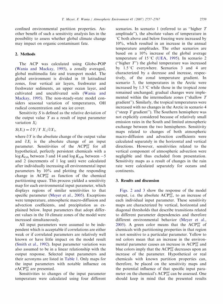
Fig. 1. The Arctic contamination potential ACP10air of perfectly

persistent organic chemicals as a function of the chemical

partitioning space defined by logKAW and logKOA.

T. Meyer, F. Wania / Atmospheric Environment 41 (2007) 2757–27672758

organic contaminants. Sensitivity analyses of suchmodels allow the identification of those inputparameters that are of the highest influence on themodel result of interest. This makes it possible todecide which input parameters and environmentalfate processes need to be known with high accuracyand precision, and for which parameters andprocesses approximate knowledge can be tolerated.We recently introduced a graphical method thatfacilitates the comprehensive investigation of modelsensitivity for all persistent organic non-electrolytesat the same time (Meyer et al., 2005). This isachieved by defining a two-dimensional hypotheti-cal ‘‘chemical partitioning space’’ as a function ofthe equilibrium partition coefficients between air,water, and octanol (KOW, KAW, KOA), and plottingsensitivity of a specific model result of eachenvironmental input parameter as a function of thischemical space. Whereas this method can be usedfor investigating the sensitivity of any predictionobtained with any linear fate model that charac-terizes the partitioning behavior of organic chemi-cals with KAW, KOW and KOA, it is most useful whena highly aggregated model result is calculated for alarge number of diverse chemicals using a fixedenvironmental scenario.

One such model result is the Arctic contaminationpotential (ACP) (Wania, 2003, 2006) calculated withthe zonally averaged global transport model Globo-POP (Wania and Mackay, 1995). Confirming poten-tial for long-range transport is part of the identifica-tion requirements for persistent organic pollutantsaccording to the Stockholm Convention (2001). Anumerical indicator of an organic chemical’s poten-tial to be transported to polar latitudes and toaccumulate in the Arctic ecosystem, the ACP10

air isdefined as the fraction of the globally emittedamount of a substance that is present within Arcticsurface media after 10 years of steady emissions tothe atmosphere (Wania, 2003, 2006). The emissionsare assumed to be spatially distributed according tothe human population. To identify which partition-ing properties favor the accumulation of an organicsubstance in polar regions, Wania (2003) calculatedthe ACP10

air for perfectly persistent hypotheticalchemicals of variable KOA and KAW and plotted theresults as a function of the chemical partitioningspace (Fig. 1). Regions of elevated ACP10

air (red)within the space can be clearly distinguished fromregions of low ACP10

air (green).The Globo-POP model relies on a large number

of spatially and temporally variable environmental

input parameters. Since these parameters describevery large and diverse climate zones, they aresubject to large variability and the values used inthe calculation are therefore subject to considerableuncertainty. Furthermore, although some environ-mental parameters are allowed to vary in time on aseasonal scale, the Globo-POP model generally doesnot account for interannual variability in environ-mental parameters, adding further uncertainty. Ananalysis of the sensitivity to environmental inputparameters should shed light on the robustness ofthe ACP10

air results, i.e. should reveal to what extentthe results depend on a particular selection of inputparameters. In a preliminary analysis, the sensitivityof the ACP10

air value for five hypothetical chemicalsto changes in environmental input parameters wasfound to be very dependent on their partitioningproperties (Wania, 2003).

Here, we use the graphical method by Meyer et al.(2005) to further explore how the environmentalinput parameters of the Globo-POP model influencethe ACP10

air value calculated for all perfectly persis-tent chemicals within the relevant range of thepartitioning space. In particular, we aim to identifythe environmental fate processes of greatest sig-nificance for chemicals with a high potential forArctic accumulation. Such an analysis may provideguidance to other researchers that are interested indeveloping models of global contaminant transport,especially when they are interested in simulating thefate of one chemical or a group of chemicals with

ARTICLE IN PRESST. Meyer, F. Wania / Atmospheric Environment 41 (2007) 2757–2767 2759

confined environmental partition properties. An-other benefit of such a sensitivity analysis lies in thepossibility to assess whether global climate changemay impact on organic contaminant fate.

2. Methods

The ACP was calculated using Globo-POP(Wania and Mackay, 1995), a zonally averaged,global multimedia fate and transport model. Theglobal environment is divided in 10 latitudinalzones, four vertical air layers, freshwater andfreshwater sediments, an upper ocean layer, andcultivated and uncultivated soils (Wania andMackay, 1995). The non-steady-state model con-siders seasonal variation of temperatures, OHradical concentration and sea ice cover.

Sensitivity S is defined as the relative deviation ofthe output value Y as a result of input parametervariation Xi:

SðX iÞ ¼ qY=Y X i=qX i;

where qY is the absolute change of the output valueand qXi is the absolute change of an inputparameter. Sensitivities of the ACP10

air for allhypothetical, perfectly persistent chemicals with alogKOA between 3 and 14 and logKAW between �5and 2 (increments of 1 log unit) were calculatedafter individually increasing all environmental inputparameters by 10% and plotting the respondingchange in ACP10

air as function of the chemicalpartitioning space. This process yielded a sensitivitymap for each environmental input parameter, whichdisplays regions of similar sensitivities to thatspecific parameter (Meyer et al., 2005). Exceptionswere temperature, atmospheric macro-diffusion andadvection coefficients, and precipitation as ex-plained below. Input parameters that adopt differ-ent values in the 10 climate zones of the model wereincreased simultaneously.

All input parameters were assumed to be inde-pendent which is acceptable if correlations are eitherweak or if correlated parameters are relatively wellknown or have little impact on the model result(Smith et al., 1992). Input parameter variation wasalso assumed to be in a linear relationship with theoutput response. Selected input parameters andtheir acronyms are listed in Table 1. Only maps forthe input parameters with notable influence oneACP10

air are presented.Sensitivities to changes of the input parameter

temperature were calculated using four different

scenarios. In scenario 1 (referred to as ‘‘higher T

amplitude’’), the absolute values of temperature in1C both above and below freezing were increased by10%, which resulted in an increase in the annualtemperature amplitudes. The other scenarios arebased on a 10% increase of the global averagetemperature of 15 1C (UEA, 1995). In scenario 2(‘‘higher T’’) the global temperature was increasedby 1.5 1C everywhere. Scenarios 3 and 4 arecharacterized by a decrease and increase, respec-tively, of the zonal temperature gradient. Inscenario 3, the temperatures in the Arctic wereincreased by 1.5 1C while those in the tropical zoneremained unchanged; gradual changes were imple-mented within the intermediate zones (‘‘shallow T

gradient’’). Similarly, the tropical temperatures wereincreased with no changes in the Arctic in scenario 4(‘‘steep T gradient’’). The Southern hemisphere wasnot explicitly considered because of relatively smallemission rates in the South and limited atmosphericexchange between the two hemispheres. Sensitivitymaps related to changes of both atmosphericmacro-diffusion and advection coefficients werecalculated separately in the horizontal and verticaldirections. However, sensitivities related to thevertical component of atmospheric advection werenegligible and thus excluded from presentation.Sensitivity maps as a result of changes in the rainrate were calculated separately for oceans andcontinents.

3. Results and discussion

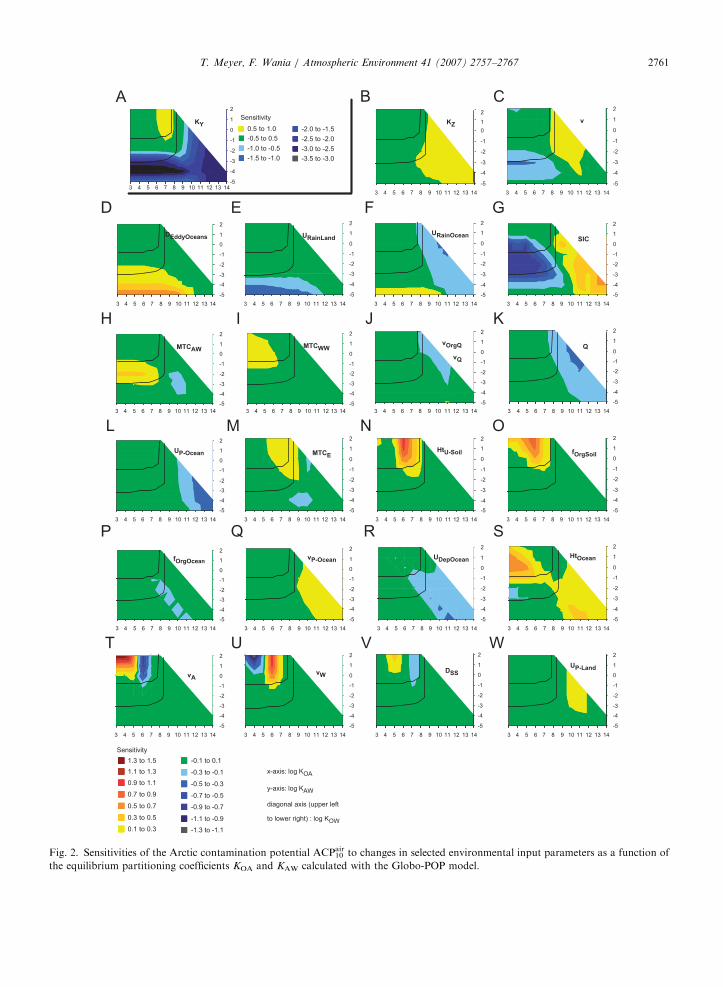
Figs. 2 and 3 show the response of the modeloutput, i.e. the absolute ACP10

air, to an increase ofeach individual input parameter. These sensitivitymaps are characterized by vertical, horizontal anddiagonal thresholds that describe transitions relatedto different parameter dependencies and thereforedifferent environmental behavior (Meyer et al.,2005). A green color means that the ACP10

air ofchemicals with partitioning properties in that regionis not sensitive to a particular parameter. Yellow tored colors mean that an increase in the environ-mental parameter causes an increase in ACP10

air andblue colors imply that the ACP10

air decreases upon anincrease of the parameter. Hypothetical or realchemicals with known partition properties can,therefore, be placed on the sensitivity maps andthe potential influence of that specific input para-meter on the chemical’s ACP10

air can be assessed. Oneshould keep in mind that the presented results

ARTICLE IN PRESS

Table 1

Model input parameters and their acronyms

Environmental input parameter Acronym

Organic carbon fraction in uncultivated soil fOrgSoil

Organic carbon fraction in ocean suspended solids fOrgOcean

Depth of uncultivated soil HtU-Soil

Depth of surface ocean HtOcean

Aerosol fraction in atmosphere vQ

Organic carbon content of aerosols vOrgQ

Suspended solids in ocean waters vP-Ocean

Fraction of water in soil pore space vWFraction of air in soil pore space vARain rate over continents URainLand

Rain rate over oceans URainOcean

Particle settling rate UDepOcean

Eddy diffusion in oceans DEddyOcean

Particle scavenging ratio Q

Mass transfer coefficient between air and water (air side) MTCAW

Mass transfer coefficient between air and water (water side) MTCWW

Mass transfer coefficient between soil and air (air side) MTCE

Dry deposition velocity over continents UP-Land

Dry deposition velocity over oceans UP-Ocean

Solid-phase diffusion in soil DSS

Horizontal atmospheric macro-diffusion coefficient KY

Vertical atmospheric macro-diffusion coefficient KZ

Horizontal atmospheric advection coefficient v

Sea ice cover SIC

Temperature T

T. Meyer, F. Wania / Atmospheric Environment 41 (2007) 2757–27672760

include the assumption of perfect persistence of allchemicals. However, a calculation with fairlypersistent substances with approximate half-livesin the atmosphere and in surface media of 1 weekand 3 years, respectively, result in a ACP10

air chemicalspace map similar to that shown in Fig. 1 (Wania,2006). Less persistent chemicals are not subject ofthis study and are generally of less concern for theArctic environment.

Input parameters or the environmental processesthey represent are only important in the context ofthis study if high ACP10

air values, as shown in Fig. 1,co-occur with high sensitivities to parameterchanges (Figs. 2 and 3). Within each of thesensitivity maps displayed in Figs. 2 and 3, twoblack contour lines, therefore, delineate the field ofchemical properties with default ACP10

air valueslarger than 2.5% (corresponds to values larger than65% of the maximum value in Fig. 1). Regions inthe chemical space that show a low ACP10

air are notconsidered in the discussion even if related to highparameter sensitivities. A look at the maps in Fig. 2reveals that the space in between the two blackcontour lines is often green, i.e., most of thecalculated high sensitivities do not coincide with

highest default ACP10air. High-ACP10

air chemicals aretypically semi-volatile that enables them to bereadily transferred among the gaseous, aqueousdissolved and particulate phases of the environ-ment. Those ‘‘multiple hoppers’’ may move betweenatmosphere and Earth’s surface numerous times ontheir way to the Arctic (Wania, 2006). As a result,these chemicals are exposed to a complex system ofenvironmental processes rendering their fate lessdependent on the change of only one or a fewparameter (Meyer et al., 2005).

3.1. Important parameters and processes

The atmosphere and oceans are the main globaltransport media, and atmosphere, ocean, anduncultivated soil are the major storage compart-ments. Accordingly, the majority of the inputparameters with notable sensitivities describe thesize and composition of these compartments and thedynamics of chemical transport in ocean and air(Fig. 2). Parameters related to the freshwaterenvironment have negligible influence on the ACP10

air

and are not presented or further discussed. Inciden-tally, this lends support to the simplified structure of

ARTICLE IN PRESS

cc

A B C

GFED

H I J K

OML

P Q R S

WVUT

N

Fig. 2. Sensitivities of the Arctic contamination potential ACP10air to changes in selected environmental input parameters as a function of

the equilibrium partitioning coefficients KOA and KAW calculated with the Globo-POP model.

T. Meyer, F. Wania / Atmospheric Environment 41 (2007) 2757–2767 2761

ARTICLE IN PRESS

3 6 8 10-5

-4

-3

-2

-1

0

1

2

3 5 6 7 8 9

-5

-4

-3

-2

-1

0

1

2

3 4 5 6 8-5

-4

-3

-2

-1

0

1

2

st eep T gr adi e nt

w a rm Tro p ic ( 4 )

3 4 5 6 7 8 9-5

-4

-3

-2

-1

0

1

2

steep T gradient

warm Tropic(4)

10 11 12 13 14 7 9 10 11 12 13 14

Above 2.5

2.0 to 2.5

1.5 to 2.0

1.0 to 1.5

0.5 to 1.0

-0.5 to 0.5

0.9 to 1.1

0.7 to 0.9

0.5 to 0.7

0.3 to 0.5

0.1 to 0.3

-0.1 to 0.1

higher T

amplitude (1)

0.5 to 1.5

-0.5 to 0.5

-1.5 to-0.5

-2.5 to -1.5

-3.5 to -2.5

-4.5 to -3.5

-5.5 to -4.5

higher T (2)

-0.5 to0.5

-1.5 to-0.5

-2.5 to -1.5

-3.5 to -2.5

-4.5 to -3.5

-5.5 to -4.5

shallow T gradient

warm Arctic (3)

4 5 7 9 11 12 13 14 4 10 11 12 13 14

Fig. 3. Sensitivities of the Arctic contamination potential ACP10air to changes in temperature calculated for four different scenarios as a

function of the equilibrium partitioning coefficients KOA and KAW using the Globo-POP model.

T. Meyer, F. Wania / Atmospheric Environment 41 (2007) 2757–27672762

chemical fate models, which include only the threecompartments air, ocean water, and soil in theirdescription of the global environment, e.g. Chem-Range (Scheringer, 1996).

Chemicals can reach the Arctic rapidly by atmo-spheric transport. An increase of the atmosphericmacro-diffusive exchange coefficient in the meridio-nal direction (KY, Fig. 2(A)) leads to decreasedArctic contamination of relatively water solublechemicals (logKAW around �4) and non-volatilesubstances (high KOA), i.e., substances that gener-ally undergo single-hop atmospheric transport(Wania, 2006). A separate sensitivity scale is neededto be assigned to Fig. 2(A), highlighting theparameter’s significance. A relatively large fractionof chemicals emitted within the Northern hemi-sphere is traveling with atmospheric currents south-wards to lower latitudes, is subsequently lifted tohigher altitudes, and finally finds its way towardsthe Arctic in higher atmospheric strata. An increaseof the horizontal macro-diffusion component means

that a larger fraction of a chemical is crossing theequator into the Southern hemisphere where it issubjected to precipitation scavenging and drydeposition and hence is prevented from accumulat-ing in the Arctic. Multi-hop chemicals, whichinclude many with high-ACP10

air, are much lessaffected by changes of the horizontal macro-diffusivity because they are sufficiently volatile tore-evaporate upon deposition to continue theirjourney to the Arctic. Similarly, very volatilesubstances stay within the atmosphere under allcircumstances, whereas very soluble chemicals areprimarily found in ocean water and are, therefore,not dependent on atmospheric transport. However,the ACP10 of relatively volatile chemicals withlogKOA values around 7 is increasing with largerhorizontal atmospheric macro-diffusivity (yellowarea in Fig. 2(A)). Because of their intermediatevolatility, those chemicals stay in the gas phasewithin temperate and tropical areas and may onlybe deposited by precipitation within the Arctic due

ARTICLE IN PRESST. Meyer, F. Wania / Atmospheric Environment 41 (2007) 2757–2767 2763

to their temperature dependent partitioning beha-vior. An increase of the vertical component ofmacro-diffusive mixing (KZ, Fig. 2(B)) mitigates theeffect caused by an increase of KY for particle-bound chemicals (logKOA49) because they nowreach the upper atmospheric layers faster and aretherefore less likely to be deposited by precipitation.Chemicals that are influenced by changes in KZ andKY exhibit properties similar to those responding tochanges in precipitation (see below).

Changes of the coefficient describing the hor-izontal component of atmospheric advection (v)result in a smaller ACP10 of chemicals with anintermediate logKAW around �3 (blue area inFig. 2(C)). Faster southward advective transportand hence a shorter residence time within the loweratmosphere diminishes the probability of theaffected chemicals being deposited into oceanswhere they experience the most efficient transportto the Arctic. More water soluble substances(logKAWo�5) are washed out from the atmosphereso fast that atmospheric transport becomes unim-portant, while slightly more volatile chemicals(logKAW �3 to �1) can easily re-evaporate. Like-wise, faster atmospheric advection prevents afraction of chemicals with intermediate logKOA

values (yellow area in Fig. 2(C)) from beingdeposited to the Earth’s surface where theywould be precluded from further transport to theArctic, hence the ACP10 of those chemicals in-creases. Sensitivities related to changes of thevertical atmospheric advection component (w) arenegligible.

In addition to the atmosphere, the other majorcarrier of organic contaminants to the Arctic is theocean. Intensified meridional exchange in theoceans, as expressed by an increase in the eddydiffusivities DEddyOceans, accordingly result in afaster arrival of water-soluble substances in theArctic Ocean and thus to an increased ACP10

air

(Fig. 2(D)). In fact, sensitivity to this parameter hadpreviously served in the identification of ‘‘swim-mers’’, i.e., chemicals subject to oceanic long-rangetransport (Wania, 2006).

Precipitation can efficiently transfer water solubleand particle-sorbed substances from the atmosphereto the Earth’s surface and hence is expected tostrongly influence the ACP10

air of such chemicals. Theimportance of precipitation in controlling atmo-spheric concentrations and long-range transport oflowKAW compounds has repeatedly been demon-strated (Hertwich, 2004; Muir et al., 2004; Jolliet

and Hauschild, 2005). The maps displaying sensi-tivity to an increase of rain rate (URainLand,URainOcean, Figs. 2(E) and (F)) indeed indicatedecreasing ACP10

air of chemicals with high tointermediate water solubility (relatively low KAW

value) and low volatility (high KOA value). The ACPof the latter substances is especially reduced by rainover the oceans (URainOcean, Fig. 2(F)). For sub-stances which are subject to LRT in the oceans (i.e.,with relatively low KAW value), an increase in therain rate over oceans (URainOcean, Fig. 2(F))predictably increases the ACP10

air by increasingtransfer to the main transport medium, where anincrease in the rain rate over continents (URainLand,Fig. 2(E)) has the opposite effect. Increased rainover land deposits an additional fraction of solublechemicals into the soil that could otherwise besubject to transport to the Arctic within oceans.Although not calculated here, we would not expecta high sensitivity to the rain rate for very water-soluble chemicals with logKAW values of below �7.Based on previous findings with a simpler model(Meyer et al., 2005), those chemicals are effectivelywashed out by even small amounts of rain and theirACP10

air would not be sensitive to a change in rainrates. Real substances affected by changes in rainrate include lindane, aldrin, highly chlorinatedPCBs, PBDEs and some currently used pesticides.

Variations in the parameter temperature yieldedthe highest absolute sensitivity values in this study(Fig. 3). Temperature influences the chemicaltransfer between all environmental phases becausethe partition coefficients are temperature dependent.The maps related to scenarios 2 (‘‘higher T’’) and 3(‘‘shallow T gradient’’) show similar sensitivitypatterns (Fig. 3). The temperature increase withinthe Arctic, which the two scenarios have incommon, leads to enhanced evaporation of volatileand semi-volatile substances, decreasing their pre-sence within the Arctic surface media and thuslowering their ACP10

air. Simultaneous increase oftropical temperatures (scenario 2—Fig. 2) counter-acts this trend for substances with a logKAW valueof around �3; increased evaporation from lowlatitude oceans into the atmosphere leads to theirmore efficient transport towards the Arctic.

In both scenario 1 (‘‘higher T amplitude’’) and 4(‘‘steep T gradient’’), the temperatures in lowerlatitudes are increased relative to colder areasenhancing northward atmospheric transport ofsemi-volatile chemicals. Numerous persistent or-ganic pollutants, such as low molecular weight

ARTICLE IN PRESST. Meyer, F. Wania / Atmospheric Environment 41 (2007) 2757–27672764

brominated flame retardants, PCBs, dieldrin, tox-aphene, DDT, chlordanes and a-HCH exhibitchemical properties that fall within this region ofhigh sensitivity. Increasing the zonal temperaturegradient, and in particular, the range of the annualtemperature amplitude, leads to reinforcement oftemperature-driven air/surface exchange processesof those chemicals and thus an intensification of the‘‘grass-hopper effect’’ and ultimately a higherACP10

air.Sea ice cover (SIC) and the mass transfer

coefficient between air and water (MTCAW) belongto the few input parameter that combine highdefault ACP10

air and high parameter sensitivities(Fig. 2(G) and (H)). Both influence the exchangeacross the air/ocean interface and mostly affectrelatively volatile chemicals with a logKOA below 8and an intermediate logKAW. Chemicals affected bySIC and MTCAW variations are somewhat morevolatile (i.e., have higher logKAW and lowerlogKOA values) than those influenced by precipita-tion or atmospheric currents; low molecular weightPCBs and HCB can be assigned to this region. Anincrease of MTCAW has a similar effect as anincrease of the temperature amplitude, the exchangeprocesses between oceans and atmosphere arefacilitated and the multi-hop transport towards theArctic in response to seasonal and diurnal tempera-ture variations is reinforced. SIC is the only inputparameter that describes processes mainly related tothe Arctic. In the Globo-POP model, SIC preventsdiffusive gas exchange (gas absorption and evapora-tion) within the fraction of the air–ocean interfacethat is ice covered. Wet deposition and dry particledeposition are assumed to continue, as contami-nants deposited this way may eventually—albeitwith a time delay of several years—find their wayinto the ocean during melt. Accordingly, increasingthe SIC impedes the atmosphere–Arctic Oceanexchange and decreases the ACP10

air of chemicalsthat are subjected to diffusive gas exchange (i.e.relatively volatile chemicals with intermediate log -KAW and logKOA) (blue area in Fig. 2(G)). For veryinvolatile chemicals (high logKOA), an increasingSIC increases the ACP10

air, because even thoughparticle-bound deposition to the ocean continues asbefore, re-evaporation is reduced (yellow area inFig. 2(G)). Other parameter describing the exchangeof contaminants across the air/ocean interface(MTCWW, Fig. 2(I)), in particular, those thatinfluence the deposition of particle-bound sub-stances from the atmosphere to oceans (vQ, vOrgQ,

Q, URainOcean, UP-Ocean, Fig. 2) are of less signifi-cance for chemicals with high default ACP10

air. This islargely because irreversibility of atmospheric de-position prevents particle-bound substances fromadopting high ACP10

air values (Wania, 2003).Substances with a logKOA around 8 and a high

logKAW are believed to efficiently exchange betweenatmosphere and terrestrial surfaces (Wania, 2003),which is reflected in high ACP10

air values (Fig. 1). TheACP of these substances is sensitive to a relativelylarge number of parameters, including the masstransfer coefficient between air and soil (air side)(MTCE), the soil depth (HTU-Soil), and the para-meters describing the capacity of atmosphericparticles (vQ, vOrgQ) and their wet deposition(URainLand, URainOcean, Q) (Fig. 2). The relevanceof this is somewhat questionable, because there arecurrently no known Arctic contaminants with suchpartitioning properties.

3.2. Segments of common parameter sensitivities

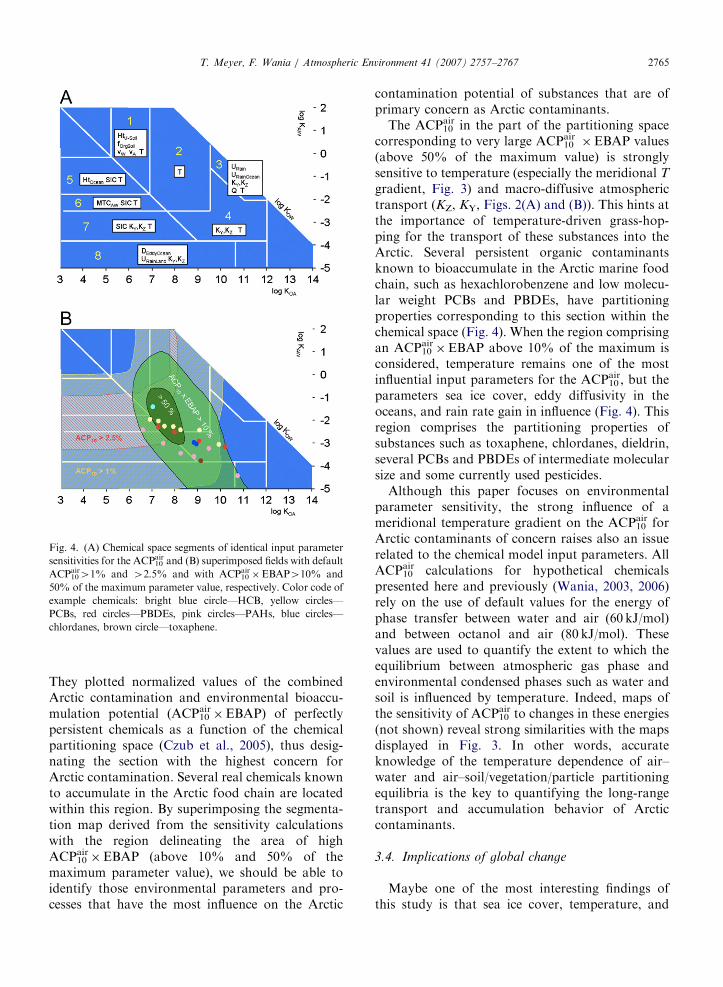
The chemical space can be segmented into areasof similar parameter sensitivities (Fig. 4(A)) with afocus on patterns and not on absolute values ofsensitivity (Meyer et al., 2005). The areas of thechemical space relating to default ACP10

air valueslarger than 1% and 2.5% are superimposedon the segmented map which enables identificationof the sensitivities for hypothetical and real chemi-cals with a high default ACP10

air (Fig. 4(B)).Chemicals with highest default ACP10

air fall insegments 2, 5, 6, and 7 (Fig. 4), where changes oftemperature and sea ice cover result in largesensitivities of the model output ACP10

air. Therelatively large segment 2 refers to chemicals thatcan be subject to intensive land–atmosphere ex-change and only temperature has a strong influenceon the ACP10

air in this segment. The major diagonalline in Fig. 4(A) suggests that sea ice cover onlybecomes important for substances with a logKOW

less than approximately 5.

3.3. Parameter sensitivities for primary Arctic

contaminants

Czub et al. (2005) coupled Globo-POP and anArctic version of the human food chain bioaccu-mulation model ACC-Human to investigate whichenvironmental partitioning properties allow organiccontaminants to both reach the Arctic and toaccumulate within the local human food chain.

ARTICLE IN PRESS

Fig. 4. (A) Chemical space segments of identical input parameter

sensitivities for the ACP10air and (B) superimposed fields with default

ACP10air41% and 42.5% and with ACP10

air�EBAP410% and

50% of the maximum parameter value, respectively. Color code of

example chemicals: bright blue circle—HCB, yellow circles—

PCBs, red circles—PBDEs, pink circles—PAHs, blue circles—

chlordanes, brown circle—toxaphene.

T. Meyer, F. Wania / Atmospheric Environment 41 (2007) 2757–2767 2765

They plotted normalized values of the combinedArctic contamination and environmental bioaccu-mulation potential (ACP10

air�EBAP) of perfectly

persistent chemicals as a function of the chemicalpartitioning space (Czub et al., 2005), thus desig-nating the section with the highest concern forArctic contamination. Several real chemicals knownto accumulate in the Arctic food chain are locatedwithin this region. By superimposing the segmenta-tion map derived from the sensitivity calculationswith the region delineating the area of highACP10

air�EBAP (above 10% and 50% of the

maximum parameter value), we should be able toidentify those environmental parameters and pro-cesses that have the most influence on the Arctic

contamination potential of substances that are ofprimary concern as Arctic contaminants.

The ACP10air in the part of the partitioning space

corresponding to very large ACP10air�EBAP values

(above 50% of the maximum value) is stronglysensitive to temperature (especially the meridional T

gradient, Fig. 3) and macro-diffusive atmospherictransport (KZ, KY, Figs. 2(A) and (B)). This hints atthe importance of temperature-driven grass-hop-ping for the transport of these substances into theArctic. Several persistent organic contaminantsknown to bioaccumulate in the Arctic marine foodchain, such as hexachlorobenzene and low molecu-lar weight PCBs and PBDEs, have partitioningproperties corresponding to this section within thechemical space (Fig. 4). When the region comprisingan ACP10

air�EBAP above 10% of the maximum is

considered, temperature remains one of the mostinfluential input parameters for the ACP10

air, but theparameters sea ice cover, eddy diffusivity in theoceans, and rain rate gain in influence (Fig. 4). Thisregion comprises the partitioning properties ofsubstances such as toxaphene, chlordanes, dieldrin,several PCBs and PBDEs of intermediate molecularsize and some currently used pesticides.

Although this paper focuses on environmentalparameter sensitivity, the strong influence of ameridional temperature gradient on the ACP10

air forArctic contaminants of concern raises also an issuerelated to the chemical model input parameters. AllACP10

air calculations for hypothetical chemicalspresented here and previously (Wania, 2003, 2006)rely on the use of default values for the energy ofphase transfer between water and air (60 kJ/mol)and between octanol and air (80 kJ/mol). Thesevalues are used to quantify the extent to which theequilibrium between atmospheric gas phase andenvironmental condensed phases such as water andsoil is influenced by temperature. Indeed, maps ofthe sensitivity of ACP10

air to changes in these energies(not shown) reveal strong similarities with the mapsdisplayed in Fig. 3. In other words, accurateknowledge of the temperature dependence of air–water and air–soil/vegetation/particle partitioningequilibria is the key to quantifying the long-rangetransport and accumulation behavior of Arcticcontaminants.

3.4. Implications of global change

Maybe one of the most interesting findings ofthis study is that sea ice cover, temperature, and

ARTICLE IN PRESST. Meyer, F. Wania / Atmospheric Environment 41 (2007) 2757–27672766

macro-diffusive atmospheric transport coefficients(and to a lesser extent precipitation rate) have thelargest impact on a persistent organic chemical’scalculated potential for Arctic accumulation. Thefate of persistent organic pollutants that areeffectively bioaccumulating in humans and mam-mals in the Arctic are mainly controlled bytemperature and atmospheric transport as well.Current scenarios of climate change imply modifi-cations in the Earth’s energy balance, temperature,ice sheet extent and sea level (Hansen et al., 2005;Bond et al., 1992) thereby also influencing pre-cipitation and atmospheric mixing patterns (Barnettet al., 2005). Thus, all of the parameters that havebeen shown to strongly influence the Arctic contam-ination behavior of persistent organic chemicals arepredicted to undergo considerable change over thenext few decades. We may thus hypothesise that theglobal transport and distribution behavior of manypersistent organic chemicals, and in particular theiraccumulation in polar marine ecosystems, may besignificantly impacted by global climate change. Thiswas previously stated by Macdonald et al. (2003) andthere is now also experimental and modellingevidence that climate fluctuations can impact onthe atmospheric transport of persistent organicpollutants (Ma et al., 2004; MacLeod et al., 2005).

Many climate change scenarios predict, andrecent observations confirm, a decreasing Arcticsea ice cover and a decreasing temperature gradientbetween Arctic and Tropics with a strongertemperature increase in colder areas compared toareas of lower latitudes (Braganza et al., 2004). Thelatter somewhat resembles temperature scenario 3‘‘shallow T gradient’’. According to our calcula-tions, a shallower temperature gradient woulddecrease the ACP10

air of Arctic contaminants ofconcern (those with partitioning properties corre-sponding to a high ACP10

air�EBAP), whereas a

reduced sea ice cover would likely increase it. Thisincidentally highlights one of the shortcomings ofthe current investigation in that it neglects theobvious link between higher Arctic temperaturesand reduced sea ice cover. Such interactions as wellas uncertainties regarding prospective changes ofrelevant input parameters currently prevent con-clusive statements as to how climate change willimpact Arctic contaminant accumulation. We sug-gest that global transport and distribution modelssuch as Globo-POP may play a role in definingmore clearly what the impact of global climatechange on global contaminant fate might be.

Acknowledgments

This work was funded by the Natural Sciencesand Engineering Research Council of Canada.

References

Barnett, T., Zwiers, F., Hegerl, G., Allen, M., Crowley, T.,

Gillett, N., Hasselmann, K., Jones, P., Santer, B., Schnur, R.,

Stott, P., Taylor, K., Tett, S., 2005. Detecting and attributing

external influences on the climate system: a review of recent

advances. Journal of Climate 18, 1291–1314.

Bond, G., Heinrich, H., Broecker, W., Labeyrie, L., McManus,

J., Andrews, J., Huon, S., Jantschik, R., Clasen, S., Simet, C.,

Tedesco, K., Klas, M., Bonani, G., Ivy, S., 1992. Evidence for

massive discharges of icebergs into the North Atlantic ocean

during the last glacial period. Nature 360, 245–249.

Braganza, K., Karoly, D.J., Hirst, A.C., Stott, P., Stouffer, R.J.,

Tett, S.F.B., 2004. Simple indices of global climate variability

and change Part II: attribution of climate change during the

twentieth century. Climate Dynamics 22, 823–838.

Climatic Research Unit, University at East Angia, Norwich UK

1995. Projections: IPCC report.

Czub, G., Wania, F., McLachlan, M.S., Identifying the persistent

organic chemicals with the highest potential for accumulation

in arctic residents. In: DIOXIN 2005, 25th International

Symposium on Halogenated Environmental Organic Pollu-

tants and POPs, Toronto, Ont., Canada, August 21–26, 2005.

Hansen, J., Nazarenko, L., Ruedy, R., Sato, M., Willis, J., Del

Genio, A., Koch, D., Lacis, A., Lo, K., Menon, S., Novakov,

T., Perlwitz, J., Russell, G., Schmidt, G.A., Tausnev, N.,

2005. Earth’s energy imbalance: confirmation and implica-

tions. Science 308, 1431–1435.

Hertwich, E.G., 2004. Intermittent rainfall in dynamic multi-

media fate modeling. Environmental Science and Technology

35, 936–940.

Jolliet, O., Hauschild, M., 2005. Modeling the influence of

intermittent rain events on long-term fate and transport of

organic air pollutants. Environmental Science and Technol-

ogy 39, 4513–4522.

Ma, J., Hung, H., Blanchard, P., 2004. How do climate

fluctuations affect persistent organic pollutant distribution

in North America? Evidence from a decade of air monitoring.

Environmental Science and Technology 38, 2538–2543.

Macdonald, R.W., Mackay, D., Li, Y.-F., Hickie, B., 2003. How

will global change affect risks from long-range transport of

persistent organic pollutants? Human and Ecological Risk

Assessment 9, 643–660.

MacLeod, M., William, J., Riley, W.J., McKone, T.E., 2005.

Assessing the influence of climate variability on atmospheric

concentrations of polychlorinated biphenyls using a global-

scale mass balance model (BETR-Global). Environmental

Science and Technology 39, 6749–6756.

Meyer, T., Wania, F., Breivik, K., 2005. Illustrating sensitivity

and uncertainty in environmental fate models using parti-

tioning maps. Environmental Science and Technology 39,

3186–3196.

Muir, D.C.G., Teixeira, C., Wania, F., 2004. Empirical and

modeling evidence of regional atmospheric transport of

currently used pesticides. Environmental Toxicology and

Chemistry 23, 2421–2432.

ARTICLE IN PRESST. Meyer, F. Wania / Atmospheric Environment 41 (2007) 2757–2767 2767

Scheringer, M., 1996. Persistence and spacial range as endpoints

of an exposure-based assessment of organic chemicals.

Environmental Science and Technology 30, 1652–1659.

Smith, A.E., Ryan, P.B., Evans, J.S., 1992. The effect of neglecting

correlations when propagating uncertainty and estimating the

population distribution of risk. Risk Analysis 12, 467–474.

Stockholm Convention on Persistent Organic Pollutants (POPs),

2001. Secretariat for the Stockholm Convention on POPs,

11–13 Chemin des Anemones, 1219 Chatelaine, Geneva,

Switzerland, URL: /www.pops.intS.

Wania, F., Mackay, D., 1995. A global distribution model for

persistent organic chemicals. Science of the Total Environ-

ment 160/161, 211–232.

Wania, F., 2003. Assessing the potential of persistent organic

chemicals for long range transport and accumulation in

Polar regions. Environmental Science and Technology 37,

1344–1351.

Wania, F., 2006. The potential of degradable organic chemicals

for absolute and relative enrichment in the Arctic. Enviro-

mental Science and Technology 40, 569–577.