What is data mining?What is data mining?What is data mining?What is data mining?

Włodzisław DuchWłodzisław Duch

Dept. of Informatics, Dept. of Informatics, Nicholas Copernicus University, Nicholas Copernicus University,

Toruń, Toruń, PolandPoland

http://www.phys.uni.torun.pl/~duchhttp://www.phys.uni.torun.pl/~duch

ISEP Porto, 8-12 July 2002

What is it about?What is it about?

• Data used to be precious! Now it is overwhelming ...Data used to be precious! Now it is overwhelming ...• In many areas of science, business and commerce In many areas of science, business and commerce

people are drowning in data.people are drowning in data.• Ex: astronomy super-telescope – data mining in Ex: astronomy super-telescope – data mining in

existing databases. existing databases.

• Database technology allows to store and retrieve large Database technology allows to store and retrieve large amounts of data of any kind.amounts of data of any kind.

• There is knowledge hidden in data. There is knowledge hidden in data. • Data analysis requires intelligence. Data analysis requires intelligence.

Ancient historyAncient history• 1960: first databases, collections of data.1960: first databases, collections of data.• 1970: RDBMS, relational data model most popular 1970: RDBMS, relational data model most popular

today, large centralized systems. today, large centralized systems. • 1980: application-oriented data models, specialized for 1980: application-oriented data models, specialized for

scientific, geographic, engineering data, time series, scientific, geographic, engineering data, time series, text, object-oriented models, distributed databases.text, object-oriented models, distributed databases.

• 1990: multimedia and Web databases, data 1990: multimedia and Web databases, data warehousing (subject-oriented DB for decision warehousing (subject-oriented DB for decision support), and on-line analytical processing (OLAP), support), and on-line analytical processing (OLAP), deduction and verification of hypothetical patterns. deduction and verification of hypothetical patterns.

• Data mining: first conference in 1989, book 1996, Data mining: first conference in 1989, book 1996, discover something useful!discover something useful!

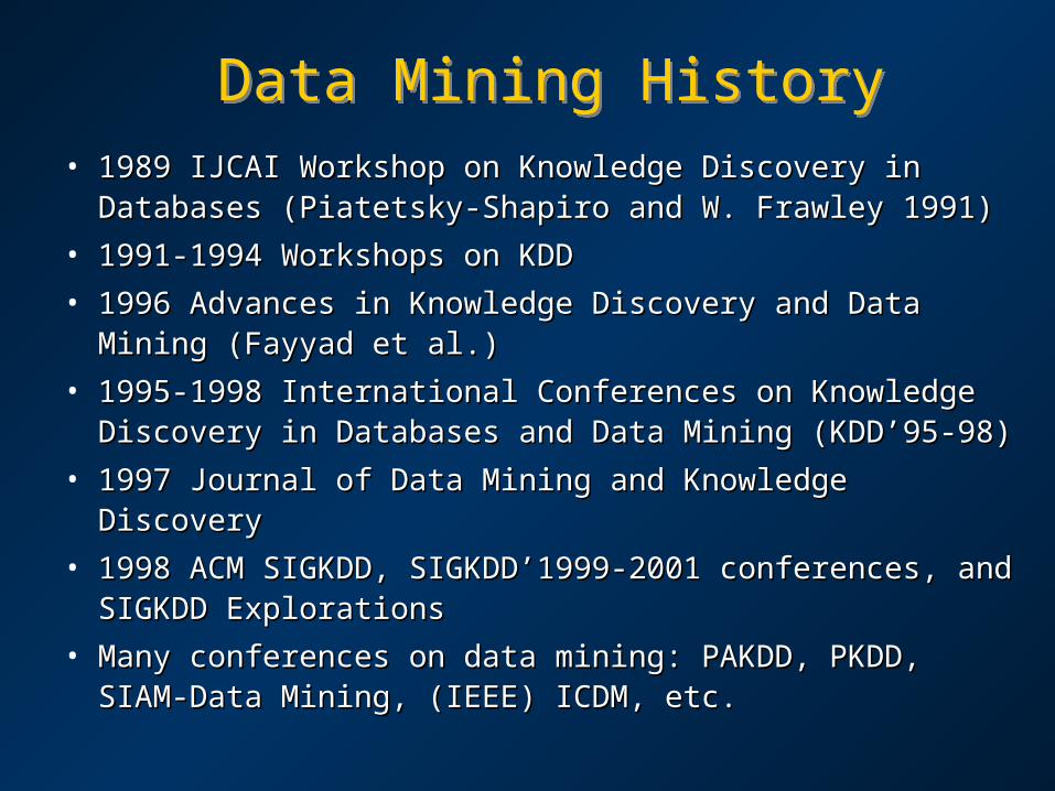
Data Mining HistoryData Mining History• 1989 IJCAI Workshop on Knowledge Discovery in 1989 IJCAI Workshop on Knowledge Discovery in

Databases (Piatetsky-Shapiro and W. Frawley 1991)Databases (Piatetsky-Shapiro and W. Frawley 1991)

• 1991-1994 Workshops on KDD1991-1994 Workshops on KDD

• 1996 Advances in Knowledge Discovery and Data Mining 1996 Advances in Knowledge Discovery and Data Mining (Fayyad et al.)(Fayyad et al.)

• 1995-1998 International Conferences on Knowledge 1995-1998 International Conferences on Knowledge Discovery in Databases and Data Mining (KDD’95-98)Discovery in Databases and Data Mining (KDD’95-98)

• 1997 Journal of Data Mining and Knowledge Discovery1997 Journal of Data Mining and Knowledge Discovery

• 1998 ACM SIGKDD, SIGKDD’1999-2001 conferences, 1998 ACM SIGKDD, SIGKDD’1999-2001 conferences, and SIGKDD Explorationsand SIGKDD Explorations

• Many conferences on data mining: PAKDD, PKDD, SIAM-Many conferences on data mining: PAKDD, PKDD, SIAM-Data Mining, (IEEE) ICDM, etc.Data Mining, (IEEE) ICDM, etc.

References, papersReferences, papers

KDD WWW Resources:KDD WWW Resources:http://www.kdd.orghttp://www.kdd.orghttp://www.kdnuggets.comhttp://www.kdnuggets.comhttp://www.the-data-mine.comhttp://www.the-data-mine.comhttp://www.acm.org/sigkdd/http://www.acm.org/sigkdd/

ResearchIndex: ResearchIndex: http://http://citeseer.nj.nec.com/csciteseer.nj.nec.com/cs

AI & ML aspectsAI & ML aspects

http://www.phys.uni.torun.pl/kmkhttp://www.phys.uni.torun.pl/kmk

NN & StatisticsNN & Statistics

http://www.phys.uni.torun.pl/kmkhttp://www.phys.uni.torun.pl/kmk

Comparison of results on many datasets:Comparison of results on many datasets:

http://www.phys.uni.torun.pl/kmkhttp://www.phys.uni.torun.pl/kmk

Data Mining and statisticsData Mining and statisticsData Mining and statisticsData Mining and statistics

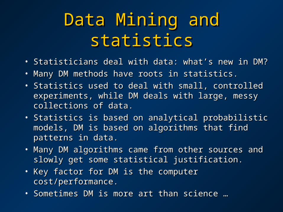
• Statisticians deal with data: what’s new in DM?Statisticians deal with data: what’s new in DM?• Many DM methods have roots in statistics.Many DM methods have roots in statistics.• Statistics used to deal with small, controlled Statistics used to deal with small, controlled

experiments, while DM deals with large, messy experiments, while DM deals with large, messy collections of data.collections of data.

• Statistics is based on analytical probabilistic models, Statistics is based on analytical probabilistic models, DM is based on algorithms that find patterns in data. DM is based on algorithms that find patterns in data.

• Many DM algorithms came from other sources and Many DM algorithms came from other sources and slowly get some statistical justification. slowly get some statistical justification.

• Key factor for DM is the computer cost/performance. Key factor for DM is the computer cost/performance. • Sometimes DM is more art than science … Sometimes DM is more art than science …

Types of DataTypes of DataTypes of DataTypes of Data

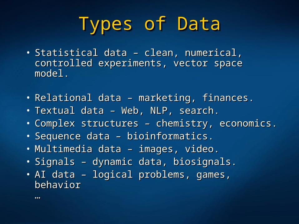
• Statistical data – clean, numerical, controlled Statistical data – clean, numerical, controlled experiments, vector space model. experiments, vector space model.

• Relational data – marketing, finances. Relational data – marketing, finances. • Textual data – Web, NLP, search. Textual data – Web, NLP, search. • Complex structures – chemistry, economics. Complex structures – chemistry, economics. • Sequence data – bioinformatics. Sequence data – bioinformatics. • Multimedia data – images, video. Multimedia data – images, video. • Signals – dynamic data, biosignals. Signals – dynamic data, biosignals. • AI data – logical problems, games, behavior AI data – logical problems, games, behavior

……

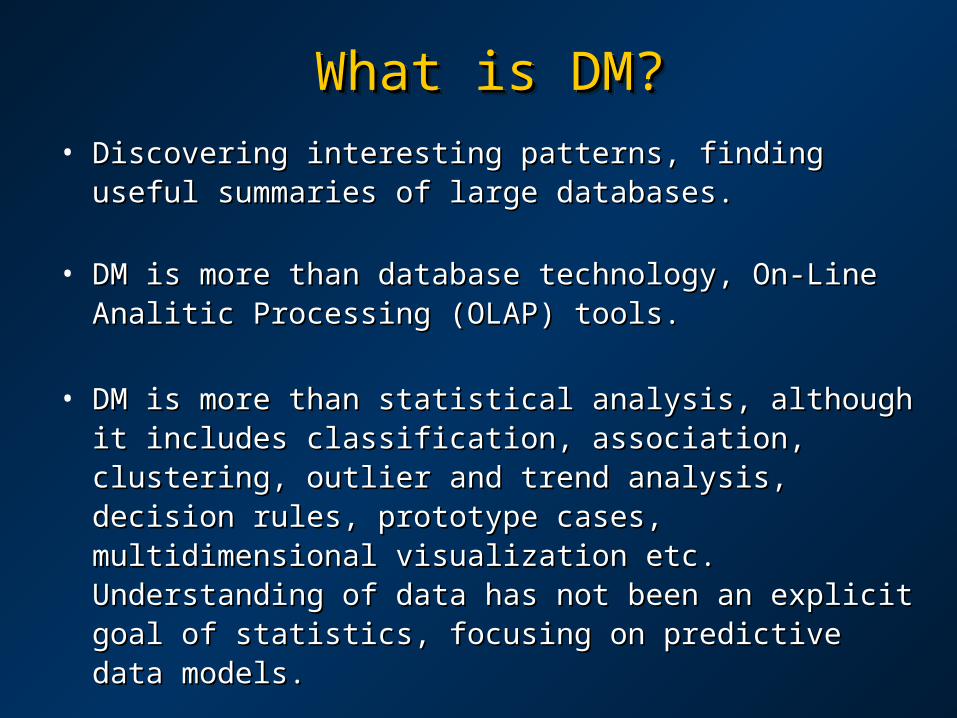
What is What is DMDM??What is What is DMDM??• Discovering interesting patterns, finding useful Discovering interesting patterns, finding useful

summaries of large databases. summaries of large databases.

• DM is more than database technology, On-Line DM is more than database technology, On-Line Analitic Processing (OLAP) tools.Analitic Processing (OLAP) tools.

• DM is more than statistical analysis, although it DM is more than statistical analysis, although it includes classification, association, clustering, includes classification, association, clustering, outlier and trend analysis, decision rules, outlier and trend analysis, decision rules, prototype cases, multidimensional visualization prototype cases, multidimensional visualization etc. Understanding of data has not been an etc. Understanding of data has not been an explicit goal of statistics, focusing on predictive explicit goal of statistics, focusing on predictive data models.data models.

DMDM applications applicationsDMDM applications applications• Many applications, but spectacular new knowledge is Many applications, but spectacular new knowledge is

rarely discovered. rarely discovered.

Some examples: Some examples:

– ““Diapers and beer” correlation: please them close and Diapers and beer” correlation: please them close and put potato chips in between. put potato chips in between.

– Mining astronomical catalogs (Skycat, Sloan Sky Mining astronomical catalogs (Skycat, Sloan Sky survey): new subtype of stars has been discovered!survey): new subtype of stars has been discovered!

– Bioinformatics: more precise characterization of some Bioinformatics: more precise characterization of some diseases, many discoveries to be made? diseases, many discoveries to be made?

– Credit card fraud detection (HNC company). Credit card fraud detection (HNC company).

– Discounts of air/hotel for frequent travelers.Discounts of air/hotel for frequent travelers.

Important issues in data mining.Important issues in data mining.Important issues in data mining.Important issues in data mining.

• Use of statistical and CI methods for KDD.Use of statistical and CI methods for KDD.

• What makes an interesting pattern? What makes an interesting pattern?

• Handling uncertainty in the data.Handling uncertainty in the data.

• Handling noise, outliers and missing or unknown data. Handling noise, outliers and missing or unknown data.

• Finding linguistic variables, discretization of continuous Finding linguistic variables, discretization of continuous data, presentation and evaluation of knowledge.data, presentation and evaluation of knowledge.

• Knowledge representation for structural data, Knowledge representation for structural data, heterogeneous information, textual databases & NLP. heterogeneous information, textual databases & NLP.

• Performance, scalability, distributed data, incremental or Performance, scalability, distributed data, incremental or “on-line” processing.“on-line” processing.

• Best form of explanation depends on the application.Best form of explanation depends on the application.

DMDM dangers dangersDMDM dangers dangers• If there are too many conclusions to draw some If there are too many conclusions to draw some

inferences will be true by chance due to too small data inferences will be true by chance due to too small data samples (Bonferroni’s theorem).samples (Bonferroni’s theorem).

Example 1: David Rhine (Duke Univ) ESP tests. Example 1: David Rhine (Duke Univ) ESP tests. 1 person in 1000 guessed correctly color (red or black) of 1 person in 1000 guessed correctly color (red or black) of 10 cards: is this evidence for ESP?10 cards: is this evidence for ESP?Retesting of these people gave average results. Retesting of these people gave average results. Rhine’s conclusion: telling people that they have ESP Rhine’s conclusion: telling people that they have ESP interferes with their ability … interferes with their ability …

Example 2: using Example 2: using mm letters to form a random sequence of letters to form a random sequence of the length the length NN all possible subsequences of log all possible subsequences of logmmN N are found are found

=> Bible code!=> Bible code!

Knowledge discovery in databases (KDD): Knowledge discovery in databases (KDD): a search process for understandable and useful a search process for understandable and useful patterns in data. patterns in data.

Data Mining

Clean,Collect,Summarize

DataWarehouse

Data Preparation

TrainingData

ModelPatterns

Verification, EvaluationOperational

Databases

Data Mining processData Mining processData Mining processData Mining process

most effort

Stages of DM processStages of DM processStages of DM processStages of DM process• Data gathering, data warehousing, Web crawling.Data gathering, data warehousing, Web crawling.

• Preparation of the data: cleaning, removing outliers and Preparation of the data: cleaning, removing outliers and impossible values, removing wrong records, finding impossible values, removing wrong records, finding missing data. missing data.

• Exploratory data analysis: visualization of different Exploratory data analysis: visualization of different aspects of data.aspects of data.

• Finding relevant features for questions that are asked, Finding relevant features for questions that are asked, preparing data structures for predictive methods, preparing data structures for predictive methods, converting symbolic values to numerical representation. converting symbolic values to numerical representation.

• Pattern extraction, discovery, rules, prototypes. Pattern extraction, discovery, rules, prototypes.

• Evaluation of knowledge gained, finding useful patterns, Evaluation of knowledge gained, finding useful patterns, consultation with experts. consultation with experts.

Multidimensional Data CuboidsMultidimensional Data Cuboids• Data warehouses use multidimensional data model. Data warehouses use multidimensional data model.

• Projections (views) of data on different dimensions Projections (views) of data on different dimensions

(attributes) form “data cuboids”. (attributes) form “data cuboids”.

• In DB warehousing literature: In DB warehousing literature:

base cuboid: original data, N-Dim. base cuboid: original data, N-Dim.

apex cuboid: 0-D cuboid, highest-level summary;apex cuboid: 0-D cuboid, highest-level summary;

data cube: lattice of cuboids.data cube: lattice of cuboids.

• Ex: Sales data cube, viewed in multiple dimensionsEx: Sales data cube, viewed in multiple dimensions– Dimension tables, ex. item (item_name, brand, type), or Dimension tables, ex. item (item_name, brand, type), or

time(day, week, month, quarter, year) time(day, week, month, quarter, year)

– Fact tables, measures (such as cost), and keys to each of the Fact tables, measures (such as cost), and keys to each of the

related dimension tablesrelated dimension tables

Data Cube: A Lattice of CuboidsData Cube: A Lattice of CuboidsData Cube: A Lattice of CuboidsData Cube: A Lattice of Cuboids

time,item

time,item,location

none

time item location supplier

time,location

time,supplier

item,location

item,supplier

location,supplier

time,item,supplier

time,location,supplier

item,location,supplier

time, item, location, supplier

0-D(apex) cuboid

1-D cuboids

2-D cuboids

3-D cuboids

4-D(base) cuboid

Forms of useful knowledgeForms of useful knowledge

But ... knowledge accessible to humans is in: • symbols, • similarity to prototypes, • images, visual representations.

What type of explanation is satisfactory?Interesting question for cognitive scientists.Different answers in different fields.

AI/Machine Learning camp: Neural nets are black boxes. Unacceptable! Symbolic rules forever.

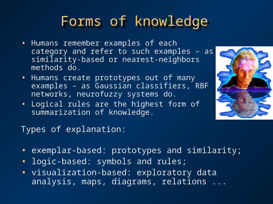
Forms of knowledgeForms of knowledge

Types of explanation:

• exemplar-based: prototypes and similarity;• logic-based: symbols and rules;• visualization-based: exploratory data

analysis, maps, diagrams, relations ...

• Humans remember examples of each category and refer to such examples – as similarity-based or nearest-neighbors methods do.

• Humans create prototypes out of many examples – as Gaussian classifiers, RBF networks, neurofuzzy systems do.

• Logical rules are the highest form of summarization of knowledge.

Computational IntelligenceComputational IntelligenceComputational IntelligenceComputational Intelligence

Computational IntelligenceData => KnowledgeArtificial Intelligence

Expert systems

Fuzzylogic

PatternRecognition

Machinelearning

Probabilistic methods

Multivariatestatistics

Visuali-zation

Evolutionaryalgorithms

Neuralnetworks

Soft computing

CI methods for data miningCI methods for data miningCI methods for data miningCI methods for data mining

• Provide non-parametric (“universal”), predictive Provide non-parametric (“universal”), predictive models of data.models of data.

• Classify new data to pre-defined categories, Classify new data to pre-defined categories, supporting diagnosis & prognosis.supporting diagnosis & prognosis.

• Discover new categories, clusters, patterns.Discover new categories, clusters, patterns.• Discover interesting associations, correlations. Discover interesting associations, correlations. • Allow to understand the data, creating fuzzy or Allow to understand the data, creating fuzzy or

crisp logical rules, or prototypes.crisp logical rules, or prototypes.• Help to visualize multi-dimensional Help to visualize multi-dimensional

relationships among data samples. relationships among data samples.

Association rulesAssociation rulesAssociation rulesAssociation rules• Classification rules: X => C(X)Classification rules: X => C(X)• Association rules: looking for correlation Association rules: looking for correlation

between components of X, i.e. probability between components of X, i.e. probability pp(X(Xii||XX11,X,Xi-1i-1,X,Xi+1i+1,X,Xnn).).

• ““Market basket” problem: many items selected Market basket” problem: many items selected from an available pool to a basket; what are the from an available pool to a basket; what are the correlations?correlations?

• Only frequent items are interesting:Only frequent items are interesting:itemsets with high support, i.e. appearing itemsets with high support, i.e. appearing together in many baskets. together in many baskets.

Search for rules above support threshold > 1%. Search for rules above support threshold > 1%.

Association rules - relatedAssociation rules - relatedAssociation rules - relatedAssociation rules - related• Related problems to market basket: Related problems to market basket:

correlation between documents – high for correlation between documents – high for plagiarism; plagiarism; phrases in documents – high for semantically phrases in documents – high for semantically related documents. related documents.

• Causal relations matter, although may be Causal relations matter, although may be difficult to determine: difficult to determine: lower the price of diapers, keep high beer price, lower the price of diapers, keep high beer price, or try the reverse – what will happen?or try the reverse – what will happen?

• More general approach: More general approach: Bayesian belief networks, causal networks, Bayesian belief networks, causal networks, graphical models. graphical models.

ClusteringClusteringClusteringClustering• Given points in multidimensional space divided them Given points in multidimensional space divided them

into groups that are “similar”. into groups that are “similar”.

• Ex: if epidemic breaks, look for location of cases on the Ex: if epidemic breaks, look for location of cases on the map (cholera in London). map (cholera in London).

Documents in the space of words cluster according to Documents in the space of words cluster according to their topics. their topics.

• How to measure similarity?How to measure similarity?• Hierarchical approaches: start from single cases, join Hierarchical approaches: start from single cases, join

them forming clusters; ex: dendrogram.them forming clusters; ex: dendrogram.

Centroid approaches: assume a few centers and adapt Centroid approaches: assume a few centers and adapt their position; ex: k-means, LVQ, SOM. their position; ex: k-means, LVQ, SOM.

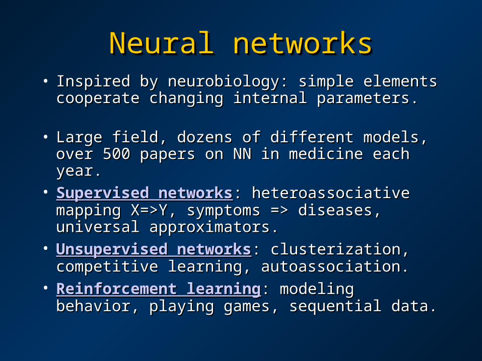
Neural networksNeural networksNeural networksNeural networks• Inspired by neurobiology: simple elements Inspired by neurobiology: simple elements

cooperate changing internal parameters.cooperate changing internal parameters.

• Large field, dozens of different models, over Large field, dozens of different models, over 500 papers on NN in medicine each year. 500 papers on NN in medicine each year.

• Supervised networksSupervised networks: heteroassociative : heteroassociative mapping X=>Y, symptoms => diseases,mapping X=>Y, symptoms => diseases,universal approximators. universal approximators.

• Unsupervised networksUnsupervised networks: clusterization, : clusterization, competitive learning, autoassociation. competitive learning, autoassociation.

• Reinforcement learningReinforcement learning: modeling behavior, : modeling behavior, playing games, sequential data.playing games, sequential data.

Unsupervised NN exampleUnsupervised NN exampleUnsupervised NN exampleUnsupervised NN exampleClustering and visualization of the quality of life Clustering and visualization of the quality of life index (UN data) by SOM map.index (UN data) by SOM map.

Poor classification, inaccurate visualization. Poor classification, inaccurate visualization.

Real and artificial neuronsReal and artificial neuronsReal and artificial neuronsReal and artificial neurons

Synapses

Axon

Dendrites

Synapses

(weights)

Nodes – artificialneurons

Signals

Neural networkNeural network for MI diagnosisfor MI diagnosisNeural networkNeural network for MI diagnosisfor MI diagnosisMyocardial Infarction~ p(MI|X)

Sex Age SmokingECG: ST

PainIntensity

PainDuration

Elevation

0.7

51 1365Inputs:

Outputweights

Inputweights

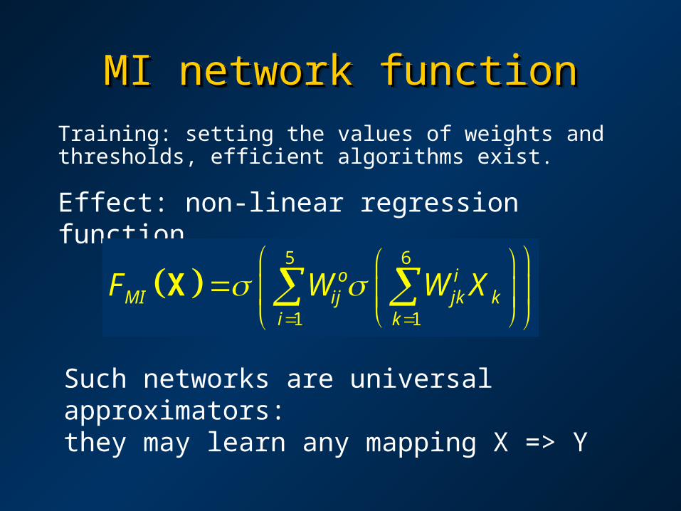
MI network functionMI network functionMI network functionMI network function

Training: setting the values of weights and thresholds, efficient algorithms exist.

Effect: non-linear regression function

Such networks are universal approximators: they may learn any mapping X => Y

5 6

1 1

o iMI ij jk k

i k

F W W X

X

Knowledge from networksKnowledge from networksKnowledge from networksKnowledge from networks

Simplify networks: force most weights to 0, quantize remaining parameters, be constructive!

• Regularization: mathematical technique improving predictive abilities of the network.• Result: MLP2LN neural networks that are equivalent to logical rules.

MLP2LNMLP2LNMLP2LNMLP2LN

Converts MLP neural networks into a network Converts MLP neural networks into a network performing logical operations (LN).performing logical operations (LN).

InputInputlayer layer

Aggregation: Aggregation: better featuresbetter features

Output: Output: one node one node per class. per class.

Rule units: Rule units: threshold logicthreshold logic

Linguistic units: Linguistic units: windows, filterswindows, filters

Learning dynamicsLearning dynamicsLearning dynamicsLearning dynamicsDecision regions shown every 200 training epochs in x3, x4 coordinates; borders are optimally placed with wide margins.

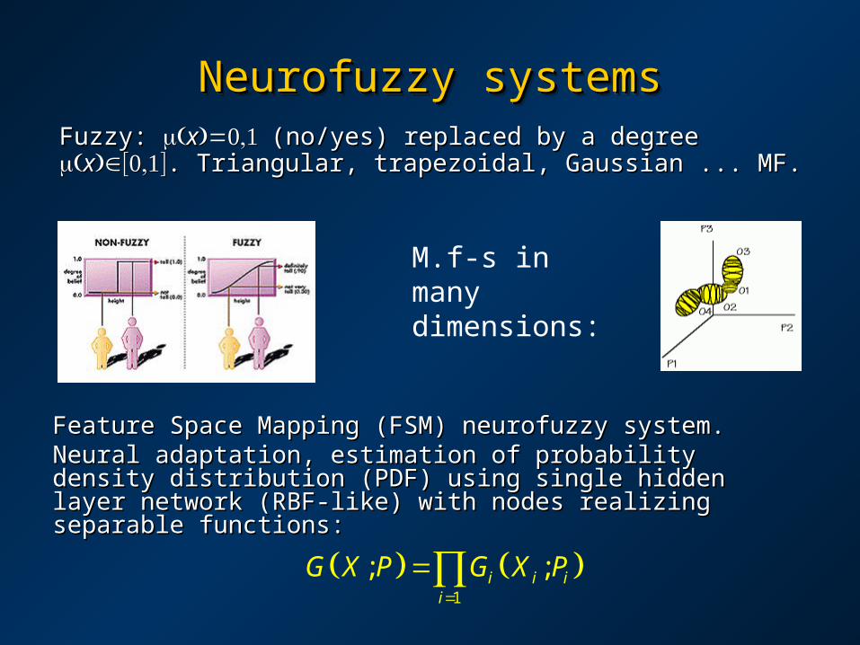
Neurofuzzy systemNeurofuzzy systemssNeurofuzzy systemNeurofuzzy systemss

Feature Space Mapping (FSM) neurofuzzy system.Feature Space Mapping (FSM) neurofuzzy system.Neural adaptation, estimation of probability density Neural adaptation, estimation of probability density distribution (PDF) using single hidden layer network distribution (PDF) using single hidden layer network (RBF-like) with nodes realizing separable functions:(RBF-like) with nodes realizing separable functions:

1

; ;i i ii

G X P G X P

Fuzzy: Fuzzy: xx(no/yes) replaced by a degree (no/yes) replaced by a degree xx. Triangular, trapezoidal, Gaussian . Triangular, trapezoidal, Gaussian ...... MFMF..

M.f-s in many dimensions:

GhostMiner PhilosophyGhostMiner Philosophy

• There is no free lunch – provide different type of tools for knowledge discovery. Decision tree, neural, neurofuzzy, similarity-based, committees.

• Provide tools for visualization of data.• Support the process of knowledge discovery/model

building and evaluating, organizing it into projects.

GhostMiner, data mining tools from our lab.

http://www.fqspl.com.pl/ghostminer/

• Separate the process of model building and knowledge discovery from model use =>

GhostMiner Developer & GhostMiner Analyzer.

Heterogeneous systemsHeterogeneous systems

• Discovering simplest class structures, its inductive bias, requires heterogeneous adaptive systems (HAS).

• Ockham razor: simpler systems are better.

• HAS examples:• NN with many types of neuron transfer functions.• k-NN with different distance functions.• DT with different types of test criteria.

Homogenous systems: one type of “building blocks”, same type of decision borders.

Ex: neural networks, SVMs, decision trees, kNNs ….

Committees combine many models together, but lead to complex models that are difficult to understand.

Wine data exampleWine data example

• alcohol content • ash content • magnesium content • flavanoids content • proanthocyanins

phenols content • OD280/D315 of diluted

wines

• malic acid content • alkalinity of ash • total phenols content • nonanthocyanins

phenols content • color intensity • hue• proline.

Chemical analysis of wine from grapes grown in the same region in Italy, but derived from three different cultivars.Task: recognize the source of wine sample.13 quantities measured, continuous features:

Exploration and visualizationExploration and visualization

General info about the data

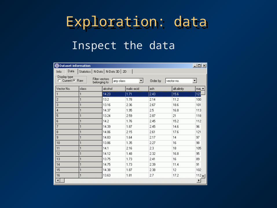
Exploration: dataExploration: data

Inspect the data

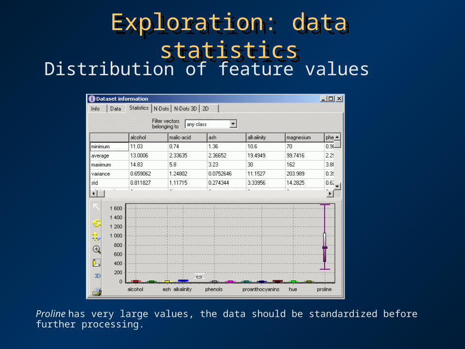
Exploration: data statisticsExploration: data statisticsDistribution of feature values

Proline has very large values, the data should be standardized before further processing.

Exploration: data standardizedExploration: data standardizedStandardized data: unit standard deviation, about 2/3 of all data should fall within [mean-std,mean+std]

Other options: normalize to fit in [-1,+1], or normalize rejecting some extreme values.

Exploration: 1D histogramsExploration: 1D histograms

Distribution of feature values in classes

Some features are more useful than the others.

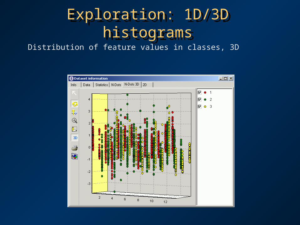
Exploration: 1D/3D histogramsExploration: 1D/3D histograms

Distribution of feature values in classes, 3D

Exploration: 2D projectionsExploration: 2D projections

Projections (cuboids) on selected 2D

Projections on selected 2D

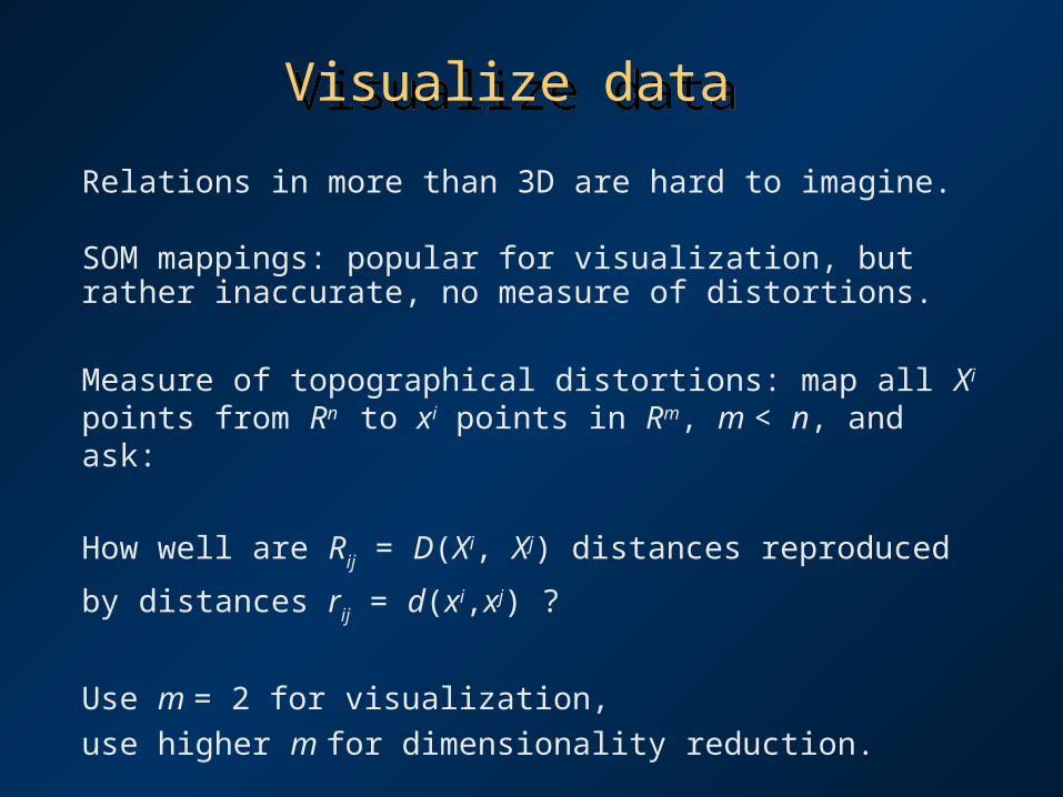
Visualize data Visualize data

Relations in more than 3D are hard to imagine.

SOM mappings: popular for visualization, but rather inaccurate, no measure of distortions.

Measure of topographical distortions: map all Xi

points from Rn to xi points in Rm, m < n, and ask:

How well are Rij = D(Xi, Xj) distances reproduced by

distances rij = d(xi,xj) ?

Use m = 2 for visualization, use higher m for dimensionality reduction.

Visualize data: MDSVisualize data: MDS

Multidimensional scaling: invented in psychometry by Torgerson (1952), re-invented by Sammon (1969) and myself (1994) … Minimize measure of topographical distortions moving the x coordinates.

2

1 2

2

2

2

3

1MDS

11Sammon

11 MDS, more local

ij iji jij

i j

ij

i jij iji j

ij iji jij

i j

S R rR

rS

R R

S r RR

x x

xx

x x

Visualize data: WineVisualize data: Wine

The green outlier can be identified easily.

3 clusters are clearly distinguished, 2D is fine.

Decision treesDecision trees

Test single attribute, find good point to split the data, separating vectors from different classes. DT advantages: fast, simple, easy to understand, easy to program, many good algorithms.

4 attributes used,

10 errors, 168 correct,

94.4% correct.

Simplest things first: use decision tree to find logical rules.

Decision bordersDecision borders

Multivariate trees: test on combinations of attributes, hyperplanes.

Result: feature space is divided into cuboids.

Wine data: univariate decision tree borders for

proline and flavanoids

Univariate trees: test the value of a single attribute x < a.

Logical rulesLogical rules

sk(x) ş True [XkŁ x ŁX'k], for example: small(x) = True{x|x < 1}medium(x) = True{x|x [1,2]}large(x) = True{x|x > 2}

Linguistic variables are used in crisp (prepositional, Boolean) logic rules:

IF small-height(X) AND has-hat(X) AND has-beard(X) THEN (X is a Brownie) ELSE IF ... ELSE ...

Crisp logic rules: for continuous x use linguistic variables (predicate functions).

Crisp logic decisionsCrisp logic decisions

True/False values jump from 0 to 1.

Step functions are used for partitioning of the feature space.

Very simple hyper-rectangular decision borders.

Sever limitation on the expressive power of crisp logical rules!

Crisp logic is based on rectangular membership functions:

Logical rules - advantagesLogical rules - advantages

• Rules may expose limitations of black box solutions.

• Only relevant features are used in rules. • Rules may sometimes be more accurate than

NN and other CI methods. • Overfitting is easy to control, rules usually

have small number of parameters. • Rules forever !?

A logical rule about logical rules is:

IF the number of rules is relatively smallAND the accuracy is sufficiently high. THEN rules may be an optimal choice.

Logical rules, if simple enough, are preferable.

Logical rules - limitationsLogical rules - limitations

Logical rules are preferred but ...

• Only one class is predicted p(Ci|X,M) = 0 or 1 black-and-white picture may be inappropriate in many applications.

• Discontinuous cost function allow only non-gradient optimization.

• Sets of rules are unstable: small change in the dataset leads to a large change in structure of complex sets of rules.

• Reliable crisp rules may reject some cases as unclassified.

• Interpretation of crisp rules may be misleading.

• Fuzzy rules are not so comprehensible.

Rules - choicesRules - choices

true | predicted r

r

p p p pp

p p p p

Accuracy (overall) A(M) = p+ p

Error rate L(M) = p+ p

Rejection rate R(M)=p+r+pr= 1L(M)A(M)

Sensitivity S+(M)= p+|+ = p++ /p+

Specificity S(M)= p = p /p

p is a hit; p false alarm; p is a miss.

Simplicity vs. accuracy. Confidence vs. rejection rate.

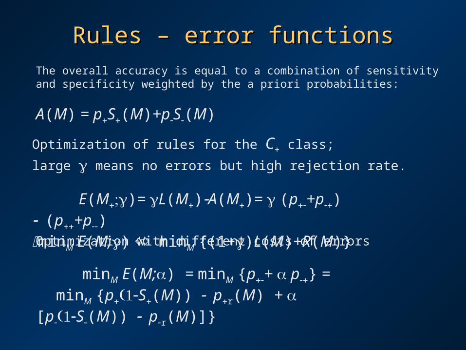
Rules – error functionsRules – error functionsThe overall accuracy is equal to a combination of sensitivity and specificity weighted by the a priori probabilities:

A(M) = pS(M)+pS(M)

Optimization of rules for the C+ class;

large means no errors but high rejection rate.

E(M)= L(M)A(M)= (p+p) (p+p)minM E(M;) minM {(1+)L(M)+R(M)} Optimization with different costs of errors

minM E(M;) = minM {p+ p} = minM {pS(M))pr(M) + [pS(M))pr(M)]}

ROC (Receiver Operating Curve): p (p, hit(false alarm).

Wine example – SSV rulesWine example – SSV rules

Decision trees provide rules of different complexity.

Simplest tree: 5 nodes, corresponding to 3 rules;

25 errors, mostly Class2/3 wines mixed.

Wine – SSV 5 rulesWine – SSV 5 rules

Lower pruning leads to more complex tree.

7 nodes, corresponding to 5 rules;

10 errors, mostly Class2/3 wines mixed.

Wine – SSV optimal rulesWine – SSV optimal rules

Various solutions may be found, depending on the search: 5 rules with 12 premises, making 6 errors, 6 rules with 16 premises and 3 errors, 8 rules, 25 premises, and 1 error.

if OD280/D315 > 2.505 proline > 726.5 color > 3.435 then class 1

if OD280/D315 > 2.505 proline > 726.5 color < 3.435 then class 2

if OD280/D315 < 2.505 hue > 0.875 malic-acid < 2.82 then class 2

if OD280/D315 > 2.505 proline < 726.5 then class 2

if OD280/D315 < 2.505 hue < 0.875 then class 3

if OD280/D315 < 2.505 hue > 0.875 malic-acid > 2.82 then class 3

What is the optimal complexity of rules? Use crossvalidation to estimate generalization.

Wine – FSM rulesWine – FSM rules

Complexity of rules depends on desired accuracy.

Use rectangular functions for crisp rules. Optimal accuracy may be evaluated using crossvalidation.

FSM discovers simpler rules, for example:

if proline > 929.5 then class 1 (48 cases, 45 correct, 2 recovered by other rules).

if color < 3.79285 then class 2 (63 cases, 60 correct)

SSV: hierarchical rulesFSM: density estimation with feature selection.

Examples of interesting knowledge discovered!Examples of interesting knowledge discovered!

The most famous example of knowledge discovered by data mining:

correlation between beer, milk and diapers.

Other examples: 2 subtypes of galactic spectra forced astrophysicist to reconsider star evolutionary processes.

Several examples of knowledge found by us in medical and other datasets follow.

MushroomsMushroomsThe Mushroom Guide: no simple rule for mushrooms; no rule like: ‘leaflets three, let it be’ for Poisonous Oak and Ivy.

8124 cases, 51.8% are edible, the rest non-edible. 22 symbolic attributes, up to 12 values each, equivalent to 118 logical features, or 2118=3.1035 possible input vectors.

Odor: almond, anise, creosote, fishy, foul, musty, none, pungent, spicySpore print color: black, brown, buff, chocolate, green, orange, purple, white, yellow.

Safe rule for edible mushrooms: odor=(almond.or.anise.or.none) Ů spore-print-color = Ř green

48 errors, 99.41% correct

This is why animals have such a good sense of smell! What does it tell us about odor receptors?

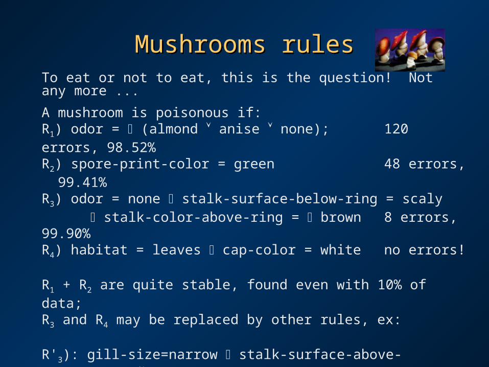
Mushrooms rulesMushrooms rulesTo eat or not to eat, this is the question! Not any more ...

A mushroom is poisonous if: R1) odor = Ř (almond anise none); 120 errors, 98.52% R2) spore-print-color = green 48 errors, 99.41% R3) odor = none Ů stalk-surface-below-ring = scaly Ů stalk-color-above-ring = Ř brown 8 errors, 99.90% R4) habitat = leaves Ů cap-color = white no errors!

R1 + R2 are quite stable, found even with 10% of data; R3 and R4 may be replaced by other rules, ex:

R'3): gill-size=narrow Ů stalk-surface-above-ring=(silky scaly) R'4): gill-size=narrow Ů population=clustered Only 5 of 22 attributes used! Simplest possible rules? 100% in CV tests - structure of this data is completely clear.

Recurrence of breast cancerRecurrence of breast cancerRecurrence of breast cancerRecurrence of breast cancer

Data from: Institute of Oncology, University Medical Center, Ljubljana, Yugoslavia.

286 cases, 201 no recurrence (70.3%), 85 recurrence cases (29.7%)

no-recurrence-events, 40-49, premeno, 25-29, 0-2, ?, 2, left, right_low, yes

9 nominal features: age (9 bins), menopause, tumor-size (12 bins), nodes involved (13 bins), node-caps, degree-malignant (1,2,3), breast, breast quad, radiation.

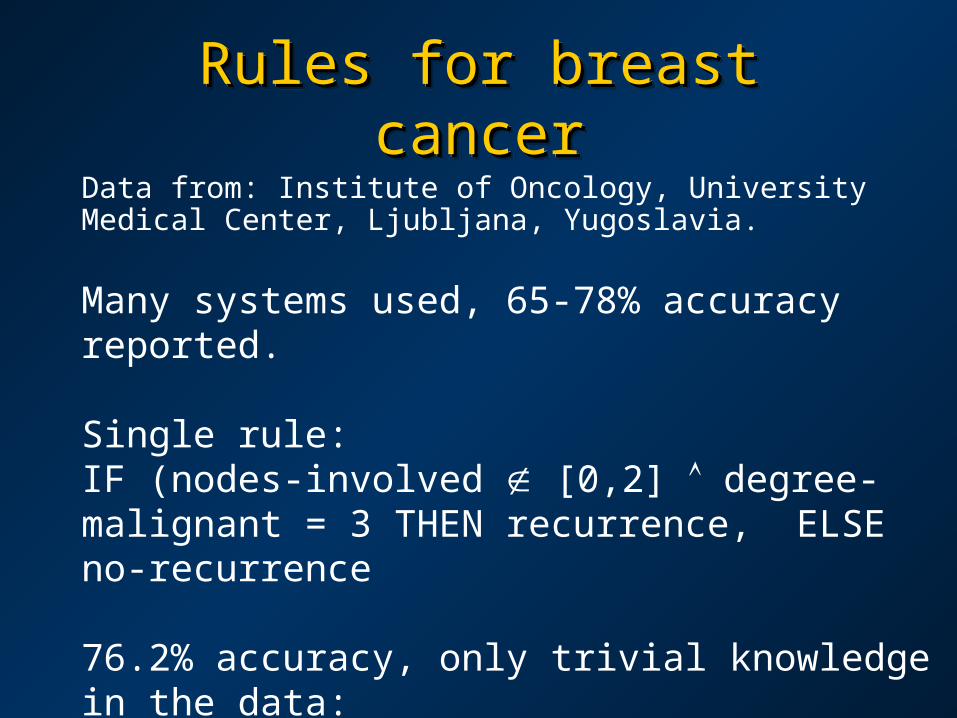
RulesRules for for breast cancerbreast cancerRulesRules for for breast cancerbreast cancer

Data from: Institute of Oncology, University Medical Center, Ljubljana, Yugoslavia.

Many systems used, 65-78% accuracy reported.

Single rule:IF (nodes-involved [0,2] degree-malignant = 3 THEN recurrence, ELSE no-recurrence

76.2% accuracy, only trivial knowledge in the data: Highly malignant breast cancer involving many nodes is likely to strike back.

Recurrence - comparison. Recurrence - comparison. Recurrence - comparison. Recurrence - comparison.

Method 10xCV accuracy

MLP2LN 1 rule 76.2 SSV DT stable rules 75.7 1.0

k-NN, k=10, Canberra 74.1 1.2

MLP+backprop. 73.5 9.4 (Zarndt)CART DT 71.4 5.0 (Zarndt) FSM, Gaussian nodes 71.7 6.8 Naive Bayes 69.3 10.0 (Zarndt)

Other decision trees < 70.0

Breast cancer diagnosis. Breast cancer diagnosis. Breast cancer diagnosis. Breast cancer diagnosis.

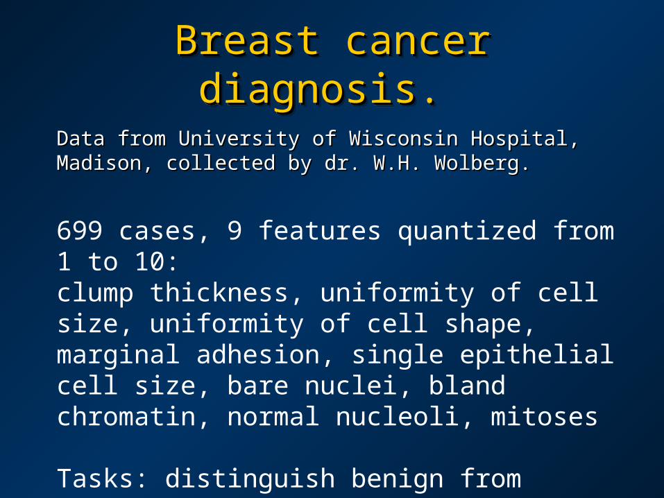
Data from University of Wisconsin Hospital, Data from University of Wisconsin Hospital, Madison, collected by dr. W.H. Wolberg.Madison, collected by dr. W.H. Wolberg.

699 cases, 9 features quantized from 1 to 10: clump thickness, uniformity of cell size, uniformity of cell shape, marginal adhesion, single epithelial cell size, bare nuclei, bland chromatin, normal nucleoli, mitoses

Tasks: distinguish benign from malignant cases.

Breast cancer rules. Breast cancer rules. Breast cancer rules. Breast cancer rules.

Data from University of Wisconsin Hospital, Data from University of Wisconsin Hospital, Madison, collected by dr. W.H. Wolberg.Madison, collected by dr. W.H. Wolberg.

Simplest rule from MLP2LN, large regularization:

If uniformity of cell size 3Then benign Else malignantSensitivity=0.97, Specificity=0.85

More complex NN solutions, from 10CV estimate:Sensitivity =0.98, Specificity=0.94

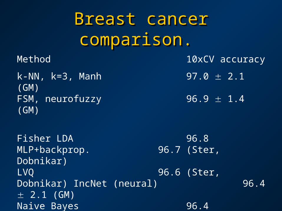
Breast cancer comparison. Breast cancer comparison. Breast cancer comparison. Breast cancer comparison.

Method 10xCV accuracy

k-NN, k=3, Manh 97.0 2.1 (GM)FSM, neurofuzzy 96.9 1.4 (GM)

Fisher LDA 96.8 MLP+backprop. 96.7 (Ster, Dobnikar)LVQ 96.6 (Ster, Dobnikar) IncNet (neural) 96.4 2.1 (GM)Naive Bayes 96.4 SSV DT, 3 crisp rules 96.0 2.9 (GM) LDA (linear discriminant) 96.0 Various decision trees 93.5-95.6

Collected in the Outpatient Center of Dermatology in Rzeszów, Poland.

Four types of Melanoma: benign, blue, suspicious, or malignant.

250 cases, with almost equal class distribution.

Each record in the database has 13 attributes: asymmetry, border, color (6), diversity (5).

TDS (Total Dermatoscopy Score) - single index

Goal: hardware scanner for preliminary diagnosis.

Melanoma skin cancerMelanoma skin cancerMelanoma skin cancerMelanoma skin cancer

R1: IF TDS ≤ 4.85 AND C-BLUE IS absent THEN MELANOMA IS Benign-nevus

R2: IF TDS ≤ 4.85 AND C-BLUE IS present THEN MELANOMA IS Blue-nevus

R3: IF TDS > 5.45 THEN MELANOMA IS Malignant

R4: IF TDS > 4.85 AND TDS < 5.45 THEN MELANOMA IS Suspicious

5 errors (98.0%) on the training set 0 errors (100 %) on the test set.

Feature aggregation is important!Without TDS 15 rules are needed.

Melanoma rules

Method Rules Training % Test %

MLP2LN, crisp rules 4 98.0 all 100

SSV Tree, crisp rules 4 97.5±0.3 100

FSM, rectangular f. 7 95.5±1.0 100

knn+ prototype selection 13 97.5±0.0 100

FSM, Gaussian f. 15 93.7±1.0 95±3.6

knn k=1, Manh, 2 features -- 97.4±0.3 100

LERS, rough rules 21 -- 96.2

Melanoma resultsMelanoma results

SummarySummarySummarySummaryData mining is a large field; only a few issues have been Data mining is a large field; only a few issues have been mentioned here. mentioned here.

DM involves many steps, here only those related to DM involves many steps, here only those related to pattern recognition were stressed, but in practice pattern recognition were stressed, but in practice scalability and efficiency issues may be most important. scalability and efficiency issues may be most important.

Neural networks are used still mostly for building predictive Neural networks are used still mostly for building predictive data models, but they may also provide simplified data models, but they may also provide simplified description in form of rules.description in form of rules.

Rules are not the only for of data understanding. Rules are not the only for of data understanding. Rules may be a beginning for a practical application. Rules may be a beginning for a practical application.

Some interesting knowledge has been discovered.Some interesting knowledge has been discovered.

ChallengesChallengesChallengesChallenges

• Discovery of theories rather than data modelsDiscovery of theories rather than data models• Integration with image/signal analysisIntegration with image/signal analysis• Integration with reasoning in complex domainsIntegration with reasoning in complex domains• Combining expert systems with neural networksCombining expert systems with neural networks

Fully automatic universal data analysis systems: Fully automatic universal data analysis systems: press the button and wait for the truth …press the button and wait for the truth …

We are slowly getting there. We are slowly getting there.

More & more computational intelligence tools More & more computational intelligence tools (including our own) are available. (including our own) are available.

DisclaimerDisclaimerDisclaimerDisclaimerA few slides/figures were taken from various presentations found in A few slides/figures were taken from various presentations found in the Internet; unfortunately I cannot identify original authors at the the Internet; unfortunately I cannot identify original authors at the moment, since these slides went through different iterations. moment, since these slides went through different iterations.

I have to apologize for that.I have to apologize for that.