WP/16/122

What’s Up with U.S. Wage Growth and Job Mobility?

by Stephan Danninger

IMF Working Papers describe research in progress by the author(s) and are published to elicit comments and to encourage debate. The views expressed in IMF Working Papers are those of the author(s) and do not necessarily represent the views of the IMF, its Executive Board, or IMF management.

© 2016 International Monetary Fund WP/16/122

IMF Working Paper

Western Hemisphere Department

What’s Up with U.S. Wage Growth and Job Mobility?

Prepared by Stephan Danninger

Authorized for distribution by Nigel Chalk

June 2016

Abstract

Since the global financial crisis, US wage growth has been sluggish. Drawing on individual earnings data from the 2000–15 Current Population Survey, I find that the drawn-out cyclical labor market repair—likely owing to low entry wages of new workers—slowed down real wage growth. There are, however, also signs of structural changes in the labor market affecting wages: for full-time, full-employed workers, the Wage-Phillips curve—the empirical relationship between wage growth and the unemployment rate—has become horizontal after 2008. Similarly, job-turnover rates have continued to decline. Job-to-job transitions—associated with higher wage growth—have slowed across all skill and age groups and beyond what local labor market conditions would imply. This raises concerns about the allocative ability of the labor market to adjust to changing economic conditions.

JEL Classification Numbers: J21, J31, J62, J63

Keywords: Labor market, Wages, Job Turnover

Author’s E-Mail Address: sdanninger@imf.org

IMF Working Papers describe research in progress by the author(s) and are published to elicit comments and to encourage debate. The views expressed in IMF Working Papers are those of the author(s) and do not necessarily represent the views of the IMF, its Executive Board, or IMF management.

3

I. INTRODUCTION

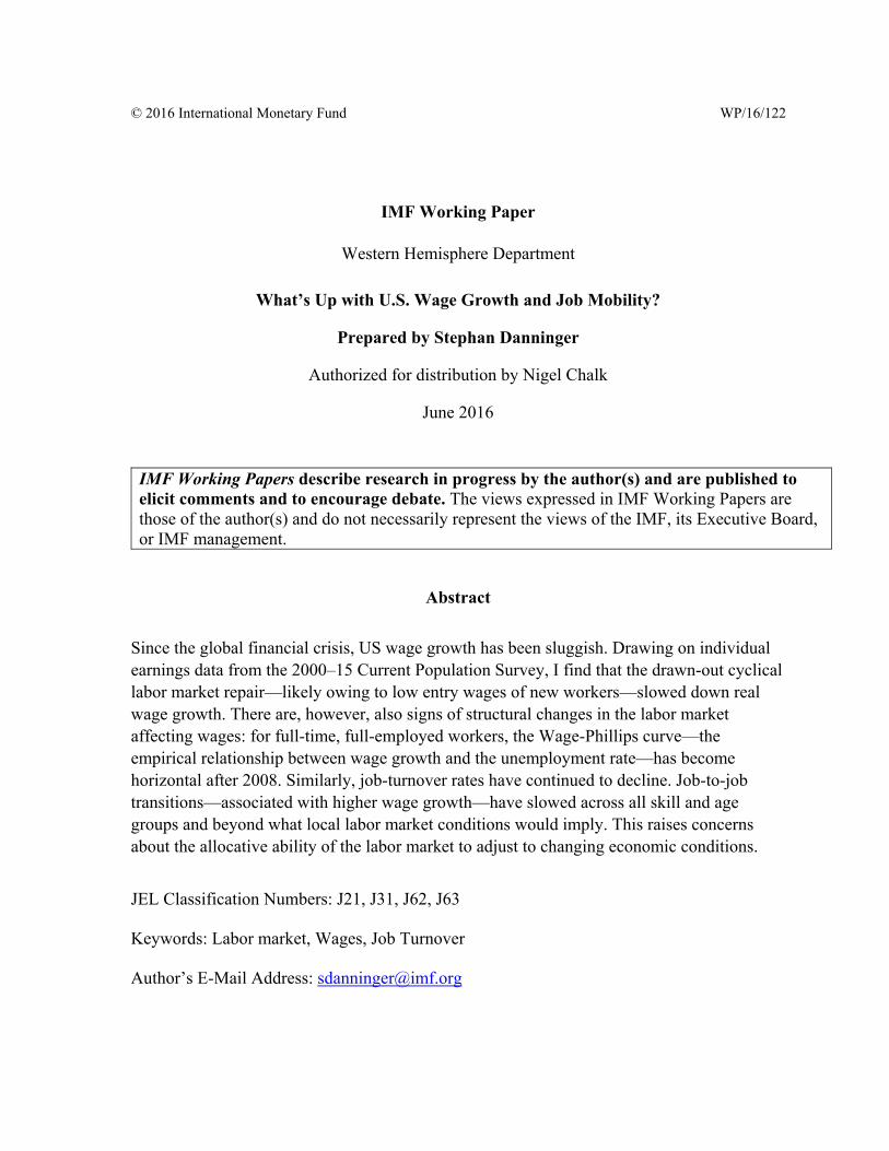
U.S wage growth has been subdued. Since 2010, annual hourly earnings in nominal terms have risen by 2 percent, about 1⅓ percent less than before the global financial crisis (GFC). Likewise, in real terms and after adjusting for differences in the slack of the labor market, wage growth has also been comparatively low (Figure 1).1 Both cyclical and structural factors have likely contributed to the slowdown. Following the GFC, businesses were left with a substantial wage hangover which has taken time to be worked out (Dent, Kapon et al 2014; Robertson 2015). In addition, the deep recession and slow recovery led to skill erosion and reduced employability of marginal workers. Once labor demand picked up and employment reached workers less attached to the labor market, low entry wages, suppressed average wage growth. Among complementary structural explanations, much recent focus has been on slowing market dynamism. Davis and Haltiwanger (2014) and Haltiwanger (2015) have pointed to a secular decline in labor market fluidity and business dynamism as possible factors. With productive firms growing less rapidly and the speed of labor reallocation across sectors flagging, technological advances permeate slower through the economy. Labor productivity has been strikingly low in recent years averaging only ½ percent during 2013–15 and moves up the wage ladder have become rarer. On the institutional side, declines in workers’ bargaining power as a result of less unionization and the emergence of alternative employment arrangements of the “gig” economy (Card and Krueger 2016; Mach and Holmes 2008) have further weighed on average income gains. To better understand the role of cyclical and structural factors, the paper poses three questions (i) is labor market repair still weighing on recent wage growth; (ii) has the relationship between labor market slack and wage growth permanently changed, i.e. has the Wage-Growth Phillips curve flattened; and (iii) focusing on job-to-job mobility, what is driving the decline in labor market churning? The main findings of the paper are: Labor market repair is still weighing on average wage growth. Exploiting regional variations in labor demand, I find that post-GFC larger declines in local unemployment rates are associated with smaller increases in average wages. Drawing on the Current Population Survey (CPS), I find that after controlling for the tightness of the local labor market, decreases (increases) in local (county-level) unemployment rates tend to reduce (raise) the average hourly wage rate in the same locality. The preferred interpretation of this effect is a moderating offset of average wage growth through the entry (exit) of low wage earners. This interpretation is consistent with recent findings that the reintegration of workers at the margins of the labor market is holding down median wage rates (Daly and Hobijn 2016).

1 Real unit labor costs, also referred to as the labor income share, have declined steadily since the early 2000s (Armenter 2015).

4

0

1

2

3

4

5

1999 2001 2003 2005 2007 2009 2011 2013 2015

Employment cost index, compensation

Average hourly earnings

Employment cost index, wages and salaries

Figure 1. United States: Average Wage Growth over Time and over the Cycle(Percent, y/y)

Source: Bureau of Labor Statistics ,CPS ,and author's calculations.

-1.0

-0.5

0.0

0.5

1.0

1.5

2.0

2.5

3.0

0.0 1.0 2.0 3.0 4.0 5.0 6.0 7.0 8.0

Real

core

avg

. hou

rly e

arni

ngs

y/y p

erce

nt ch

ange

Number of unemployed people per job opening

2004-072008-092010-112012-15

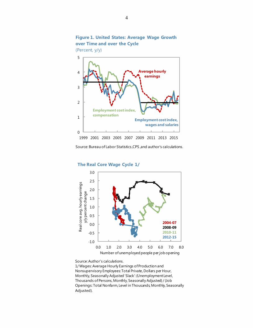
The Real Core Wage Cycle 1/

Source: Author's calculations.1/ Wages: Average Hourly Earnings of Production and Nonsupervisory Employees: Total Private, Dollars per Hour, Monthly, Seasonally Adjusted ‘Slack’: (Unemployment Level, Thousands of Persons, Monthly, Seasonally Adjusted) / (Job Openings: Total Nonfarm, Level in Thousands, Monthly, Seasonally Adjusted).

5

Second, structural changes in the labor market are also affecting wage growth. The wage-growth-Phillips curve has flattened. Declines of unemployment rates at the

state level provide a smaller boost to wage growth after the GFC than in the past. Using the CPS rotating earners’ sample, I find that after 2008 wages of full-time full-year employed do not commove with local unemployment rates, while they did prior to the GFC. Specifically, pre-2008 the Phillips curve steepened below 5 percent. Labor market data up to 2014 no longer show evidence of a similar kink in the post GFC period.

Job-to-job change rates—associated with higher wage growth—have declined well before the GFC. Using a shift-share analysis I find that post 2000 demographic changes, in particular labor force aging or changes in education, cannot account for the sustained decline in job-to-job transition rates. Rather job-to-job turnover rates have fallen in all education and age groups, irrespective of the tightness of the regional labor market. This common feature is not easily explained by more positive interpretations, such as better job matching or higher return to job tenure (Molly et al 2016).

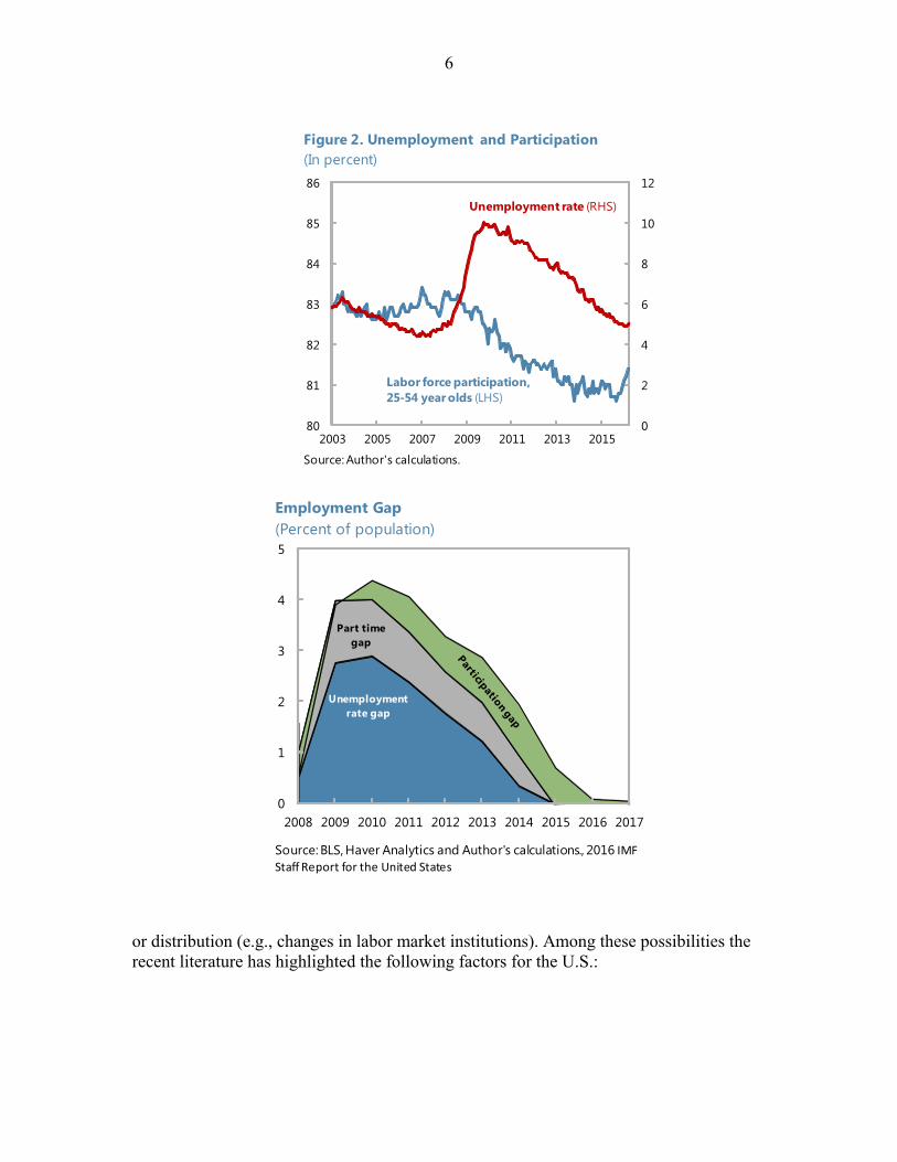
These findings have important implications for future wage growth. In the near term, as continued job growth reduces the remaining employment gap (Figure 2)—and with it headwinds from the re-employment of low-wage workers—average wage growth is expected to accelerate. However, a return to sustained high wage growth rates is uncertain. The flattening of the wage-Phillips curve post-GFC points to broader structural changes in the labor market. One possible explanation is the decline in labor market churning. By slowing down labor reallocation, productivity gains could be suppressed and thereby slow wage growth. Identifying the underlying causes for the widespread decline in job turnover is beyond the scope of this paper. Recent research is suggestive of the fact that lower market fluidity may be linked to a weakening bargaining power, which allows firms to extract rents from worker, reducing the incentive to move between jobs. New work arrangement which limit the transferability of skills could be another factor. Finally, the well documented steady decline in firm entry rates and its potential effect on productivity could be another reason for the decline in labor market mobility. The remainder of the paper is organized as follows: Section II gives a brief overview of explanations for low wage growth in the United States. Section III presents the empirical methodology and findings the empirical findings, and Section IV concludes. Details of the empirical estimates are summarized in a data annex.

II. DRIVERS OF LOW WAGE GROWTH –POSSIBLE EXPLANATIONS

Broadly speaking, changes in wage growth can result from one of two reasons: cyclical changes in labor demand or supply and/or structural changes affecting relative labor supply (e.g. migration, demographic shifts), changes in productivity (e.g., technological advances),

6

or distribution (e.g., changes in labor market institutions). Among these possibilities the recent literature has highlighted the following factors for the U.S.:

0

2

4

6

8

10

12

80

81

82

83

84

85

86

2003 2005 2007 2009 2011 2013 2015

Unemployment rate (RHS)

Labor force participation, 25-54 year olds (LHS)

Figure 2. Unemployment and Participation(In percent)

Source: Author's calculations.

0

1

2

3

4

5

2008 2009 2010 2011 2012 2013 2014 2015 2016 2017

Unemployment rate gap

Part timegap

Employment Gap(Percent of population)

Source: BLS, Haver Analytics and Author's calculations., 2016 IMF

Staff Report for the United States

7

Cyclical factors The depth of the recession and the damage to the financial and real estate sectors likely led to slower employment and wage recoveries compared to previous recessions.2 These effects may have operated through two channels: Nominal wage rigidity. Because firms cannot reduce labor costs by as much as they

would like, adjustments operate through drawn-out wage moderation. Since the GFC the share of workers with zero nominal wage growth has steadily increased (Daly, Hobijn and Ni 2013). Similarly, Daly and Hobijn (2015) find that workers in industries with larger output declines experienced a more pronounced slowdown in wage growth than in less affected industries.

Hysteresis effects. Hobijn and Pyle (2016) and Dent, Kapon, et al (2014) find that the post GFC recovery led to a compositional change of the employed labor force. The longer the labor market recovery advances, the larger has been the share of unattached of workers. Because of long periods of non-employment, their (re-)employment has been associated with substantial discounts on entry wages, thereby suppressing average hourly wage growth.

Structural factors3 Over the last two decades multifactor and labor productivity has declined steadily. In parallel the labor share in income has fallen. These two trends have given rise to several possible explanations. Changes in wage bargaining. The decline in unionization and the adoption of “Right to

work” legislation in several states have weakened the position of labor in the post GFC period (Solow 2016). In addition, new work arrangements–such as help agencies, on-call-employment and contract work– and a restructuring of office processes (Carnevale and Rose, 1998) have increased the substitutability of white-collar workers. Latest estimates put the share of workers in alternative arrangements at 16 percent, up 6 percentage points from a decade ago (Card and Krueger 2016). Finally, an estimated 18 percent of workers have wage contracts with “non-compete” clauses, which reduce the scope for intra-industry job mobility thereby limit the transferability skills across firms (Starr, Evan and Norman Bishara, 2016).

Slowing labor reallocation. Haltiwanger and Davis (2014) and Molloy, Smith, Trezzi, Wozniak (2016) document that in parallel to slowing business dynamism4 the pace of job

2 Ball (2015) argues that the because of the severity of the downturn layoffs and losses in skills were greater and hysteresis effects larger than in previous recessions. 3 Population aging and the retirement of baby boomers is another potential factor dampening wage growth, but is estimated to have had only a small effect (Ellyn and Robertson 2015). Another potential explanation is the rising share of benefits in overall labor compensation which may have led to a slowdown in pecuniary compensation through wages (Rose 2015). 4 Guzman and Scott Stern (2016) argue that although high-potential-growth startups are still growing, the ability of such startups to commercialize and scale their operations seems to be facing increasing difficulties to expand.

8

reallocation rates has declined. Empirically, the decline in job churning is related to demographic shifts, but leaves a substantial part of the decline unexplained. There is currently little consensus of factors behind the decline. Reduced mobility appears not related to improved job matching, changes in household structures (dual earners), job locks, or declines of a job-switching premia, (Hyatt and Spletzer 2013; Haltiwanger 2015). Implications for wage growth are hence unclear, but if unobserved costs of mobility have increased, then less churning could lead to lower wage growth through a slower accumulation of general skills and deteriorating job matches (Robertson 2015).

Rising global labor supply and mobility of production. Rapid growth in global goods and

services trade has generated a labor supply shock affecting US workers operating through import penetration and production shifting. Theoretically, the effects on wage growth is ambiguous as offshoring of production, for instance, can lead to higher productivity in domestic production and higher wages.

Identifying whether the above explanations are indeed structural or related to the drawn out cyclical labor market recovery is another difficulty. Less churn in recent years could be a sign of changes in transferable skills, but could also be the result of heightened job insecurity and revive as employment stability improves. Similarly, the size of alternative employment arrangements could have lifted costs of mobility. The next section lays out an empirical strategy that addresses some of these questions.

III. EMPIRICAL STRATEGY AND RESULTS

The empirical section comprises three complementary empirical exercises. In the first part, I estimate the effect of cyclical changes in local labor demand on the level of average hourly wages to explore whether compositional changes in local employment—though the entry and exit of new workers—are borne out in local wage rates. Second, I test for structural changes in the wage setting by testing whether the slope of the Wage–Phillips curves of full-employed has flattened. Finally, I assess evidence on declining job-to-job transition rates in the labor market and its underlying factors.

A. Data

The analysis uses individual‐level data from the Current Population Survey (CPS) as its source for data on wage levels as well as wage growth, with the latter being derived from the Merged Outgoing Rotation Group (MORG)5 of the CPS. The sample covers the period from

5 The CPS is a representative monthly household survey conducted by the U.S. Bureau of Labor Statistics and collects information on unemployment, labor force participation, and demographic characteristics of the population. The MORG is a subset of the full CPS sample, with detailed information for 25,000 or more individuals per month, including their employment status, earnings, as well as the age, education, race, ethnicity, and gender as well local residence of each recipient. Every household that enters the CPS is interviewed each month for 4 months, then ignored for 8 months, then interviewed again for 4 more months.

9

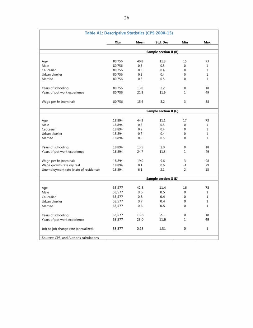
January 2000 to March 2015 and has been obtained from IPUMS-CPS website at the University of Minnesota (www.ipums.org). The main variable of interest is the real hourly wage rates, which is obtained by deflating the reported hourly wage rates of workers with the consumer price index. The study uses wage and employment data from the CPS in three different ways. In section B, I draw on an annual cross-section of employed workers to study the relationship between individual wage levels and local unemployment rates. To capture effects from labor market and exits and entries I match each worker with county unemployment rates of their respective county of residence. This dataset is substantially larger than the cross-section analyzed in section C which analyzes wage growth. In that section, I utilize the MORG data set to derive annual wage growth rates for workers with repeated (12-month apart) observations of hourly wages. Because section C analyzes the link between wage growth and unemployment more broadly, I match state-level unemployment rates to individual data..Finally, in Section D, I examine job-to-job mobility rates. For this analysis, I concentrate on a bivariate job-to-job change rate variable, measuring whether an individual obtained a new employment during the last four weeks conditional on having been fully employed during the last 12 months (definition in Annex 1). Summary statistics of the samples used in section B to D are reported in Annex 1

B. Average wages dampened by labor market repair

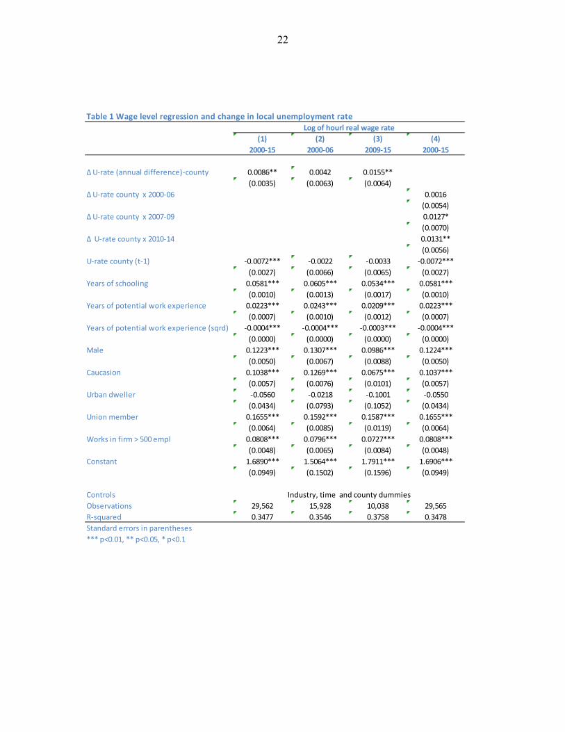
This section tries to corroborate recent empirical findings by Dale and Hobijn (2016) who estimate that changes in the composition of employed workers substantially moderated median wages. They report that 70–80 percent of new job holders post-GFC earn wages below median levels and hence lower average wages as they enter the employed workforce. As a result, despite declining unemployment rates, wage growth is likely slowed down by this compositional employment effect. This effect will likely wane as the employment gap closes and the entry of workers with comparatively low wages slows down. To estimate the size of this composition wage offset, I exploit the correlation of average wage rates across local measures of labor market slack. Because local wage rates are likely influenced by regional skill- and sector-specific demand conditions, changes in the local unemployment rate (dut/t-1 county) may be correlated with labor market entry and exit rates and, hence, affect average wages rate through changes in the composition of the employed labor force. To explore this hypothesis, I estimate an augmented log-wage regression developed by Jacob Mincer in 1973.

Usual weekly hours/earning questions are asked only at households in their 4th and 8th interview. These outgoing interviews are the only ones included in the extracts. New households enter each month, so one fourth the households are in an outgoing rotation each month. Wage rates are based on respondent’s earnings per hour in his/her current job, for workers paid an hourly wage.

10

(1) ln ωit,county = f (dut/t-1 county, ut-1, county, Xit t, county)

where ωit, county is the level of hourly earnings in year t, ut-1, county the local unemployment rate, dut/t-1, county the annual percentage point change of the county unemployment rate, and Xit worker and job characteristics including education level, years of work experience, and demographic characteristics. Specifications include year, industry, and county dummies (t, county). The analysis was conducted over the period 2000–15 and reproduces results found in the literature. A description of the variables and demographic characteristics of the sample are given in Annex 1. The estimate of interest is the coefficient on the change in the county unemployment rate. The parameter estimate can be interpreted as a measure of the compositional wage offset from a change in local demand. The assumption made is that changes in labor demand affect the composition of workers in a given locality—i.e. accelerate the entry (exit) of workers with below median wages rates—and hence slow down the change in average wage rates through a compositional discount. The results from the augmented wage regression model are reported in Table 1. Across all specifications, higher unemployment rates (U-rate county) are associated with lower hourly real wages. To assess the presence of a compositional offset, the model evaluates whether there is an additional wage resulting from changes in the unemployment rate (inducing labor market exits and entries of low paid workers). Column 1 in Table 1 shows that a decrease in the local unemployment rate by 1 percentage point–while controlling for job and worker specific characteristics—offset the increase in the average local hourly wage rate (as measures above by 0.9 percent. Splitting the sample into a pre-GFC and a post GFC period (columns 2–4) shows that the compositional effect has been substantially more pronounced after 2008. The offsetting wage level effect is substantially larger and depending on the specification ranges between 1.3-1.5 percent per one percentage point decline in the unemployment rate. This finding is consistent with the fact that exits and entries of workers with lower skills and productivity from/to employment were larger than in the past and hence affected average hourly wages to a larger degree than in the past. Specifically, the dampening effect has been symmetric (not shown): declines in average wages are lower in counties with larger increases in unemployment rates (plausibly because low wage workers dropped out at a relatively faster rate). During the labor market recovery period, counties with larger declines in unemployment rates saw comparatively lower average wage levels, possibly a result of the low entry wages of unemployed and non-participants.

C. A flattening of the wage-growth Phillips curve

In a next step, I explore the determinants of wage growth among continuously employed workers. This group of the employed labor force accounts for about two-thirds of all employed workers and is responsible for over 90 percent of labor earnings. This section explores whether for this group of workers the cyclical response of wage growth has become

11

weaker since the GFC. More specifically, we explore whether wage growth relative to past economic cycles is less sensitive to the unemployment rate.

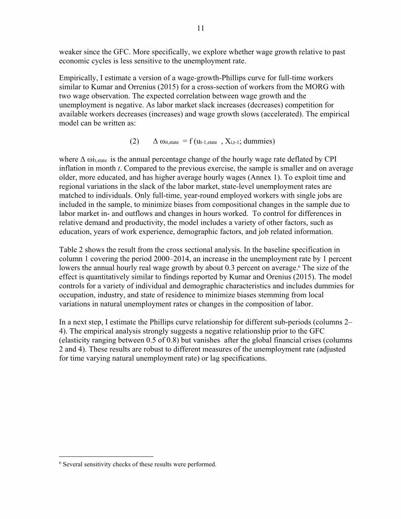
Empirically, I estimate a version of a wage-growth-Phillips curve for full-time workers similar to Kumar and Orrenius (2015) for a cross-section of workers from the MORG with two wage observation. The expected correlation between wage growth and the unemployment is negative. As labor market slack increases (decreases) competition for available workers decreases (increases) and wage growth slows (accelerated). The empirical model can be written as:

(2) Δ ωit,state = f (ut-1,state , Xi,t-1; dummies)

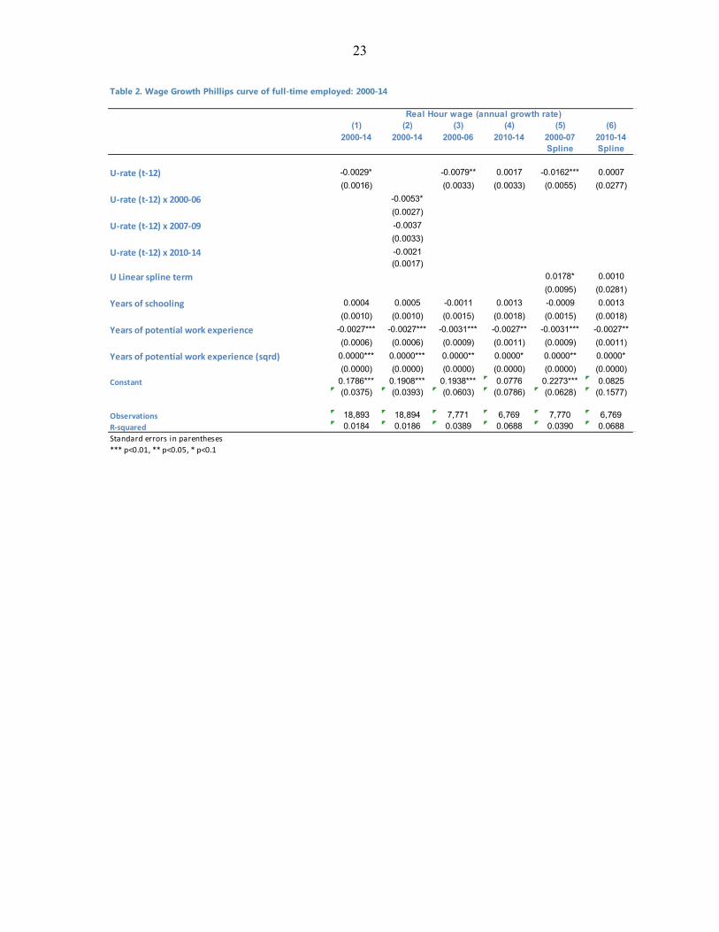
where Δ ωit,state is the annual percentage change of the hourly wage rate deflated by CPI inflation in month t. Compared to the previous exercise, the sample is smaller and on average older, more educated, and has higher average hourly wages (Annex 1). To exploit time and regional variations in the slack of the labor market, state-level unemployment rates are matched to individuals. Only full-time, year-round employed workers with single jobs are included in the sample, to minimize biases from compositional changes in the sample due to labor market in- and outflows and changes in hours worked. To control for differences in relative demand and productivity, the model includes a variety of other factors, such as education, years of work experience, demographic factors, and job related information. Table 2 shows the result from the cross sectional analysis. In the baseline specification in column 1 covering the period 2000–2014, an increase in the unemployment rate by 1 percent lowers the annual hourly real wage growth by about 0.3 percent on average.6 The size of the effect is quantitatively similar to findings reported by Kumar and Orenius (2015). The model controls for a variety of individual and demographic characteristics and includes dummies for occupation, industry, and state of residence to minimize biases stemming from local variations in natural unemployment rates or changes in the composition of labor. In a next step, I estimate the Phillips curve relationship for different sub-periods (columns 2–4). The empirical analysis strongly suggests a negative relationship prior to the GFC (elasticity ranging between 0.5 of 0.8) but vanishes after the global financial crises (columns 2 and 4). These results are robust to different measures of the unemployment rate (adjusted for time varying natural unemployment rate) or lag specifications.

6 Several sensitivity checks of these results were performed.

12

In a final step, I explore whether there is evidence of a non-linear relationship, by estimating a linear spline model with a break point at the pre 2007 average unemployment rate of 5 percent. Given the above findings, I estimate two curves: one for the pre- and one for the post-GFC period. The findings are reported in the final two columns of Table 2. During the pre-GFC period, the wage growth elasticity is substantially larger once the unemployment rate slips below the 5 percent threshold with an elasticity of -1.6, implying a growth boost of 1½ percent for every one-percent decline of the unemployment rate below 5 percent. This effect is, however, not present in the post GFC period where the Phillips curve has flattened over the whole segment of unemployment rates (Figure 4, red versus green lines).7 Arguably though, post GFC the unemployment rate has only been a short time below the natural rate (which could now be below 5 percent) and hence empirically it may be difficult to detect a kink at this time. Given these considerations, we look in the next section at changes in labor mobility to explore other evidence for structural changes in the labor market.

D. Declining job-to-job change rates

Several studies have documented a steady decline of job mobility. For several decades measures of labor churning—turnover rates exceeding job-creation and destruction rates—have decreased (Haltiwanger 2015). An important element of this change has been a decline in the frequency of job-to-job moves, a transition from one to another employment without entering unemployment. These changes are often linked to wage growth (Faberman and Justiniano 2015). During tight labor markets, job switching permits workers to capitalize on increased demand for labor. But also under normal demand conditions, job-to-job moves can generate higher earnings by improving job-worker matches and through the reallocation of

7 The results post-GFC could be biased downwards by the limited number of observation of unemployment rates below 5 percent. That said, the flatness of the post-GFC wage-growth Phillips curve is robust to the choice of higher Pivot points that is break points for the slope of the Phillips curve.

-0.15

-0.1

-0.05

0

0.05

0.1

0.15

-0.15

-0.1

-0.05

0

0.05

0.1

0.15

1 2 3 4 5 6 7 8 9

Wag

e g

row

th r

ate

Figure 3. Wage Phillips curveLinear Spline: Pivot U-rate=5 percent

pre GFC

Post GFC

95%confidenceintervall

13

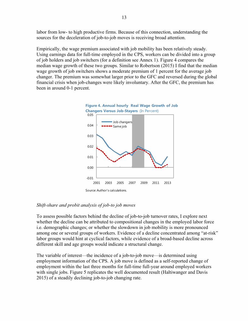
labor from low- to high productive firms. Because of this connection, understanding the sources for the deceleration of job-to-job moves is receiving broad attention. Empirically, the wage premium associated with job mobility has been relatively steady. Using earnings data for full-time employed in the CPS, workers can be divided into a group of job holders and job switchers (for a definition see Annex 1). Figure 4 compares the median wage growth of these two groups. Similar to Robertson (2015) I find that the median wage growth of job switchers shows a moderate premium of 1 percent for the average job changer. The premium was somewhat larger prior to the GFC and reversed during the global financial crisis when job-changes were likely involuntary. After the GFC, the premium has been in around 0-1 percent.

Shift-share and probit analysis of job-to job moves To assess possible factors behind the decline of job-to-job turnover rates, I explore next whether the decline can be attributed to compositional changes in the employed labor force i.e. demographic changes; or whether the slowdown in job mobility is more pronounced among one or several groups of workers. Evidence of a decline concentrated among “at-risk” labor groups would hint at cyclical factors, while evidence of a broad-based decline across different skill and age groups would indicate a structural change.

The variable of interest—the incidence of a job-to-job move—is determined using employment information of the CPS. A job move is defined as a self-reported change of employment within the last three months for full-time full-year around employed workers with single jobs. Figure 5 replicates the well documented result (Haltiwanger and Davis 2015) of a steadily declining job-to-job changing rate.

-0.01

0.00

0.01

0.02

0.03

0.04

0.05

2001 2003 2005 2007 2009 2011 2013

Job changersSame job

Figure 4. Annual hourly Real Wage Growth of Job Changers Versus Job-Stayers (In Percent)

Source: Author's calculations.

14

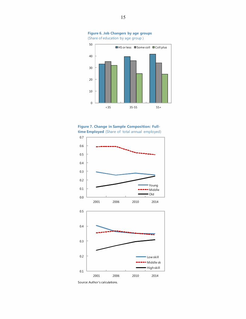
The shift-share analysis decomposes the decline in the overall job-to-job changing rate (jj) at time t with respect to a base year 0. It can be approximated as the sum of (a) changes in the population share of each group (s) weighted by their base-year job-to-job change rate (the so-called population share shift or “demographic effect”); and (b) changes in the job-to-job turnover rate of each group, g, weighted by their base-year population share (the so-called job-to-job change shift): (3) jj jj ∑ jj s s s jj jj The decomposition is carried out for the period 2000–2014 and distinguishes between three skill and age groups. The skill groups comprise workers with high school or less education, workers with some but less than a four year of college education, and workers with a college or higher degree. By age, the sample is divided into an under 35 years of age group representing Millennials, a middle age group of 35–55 year olds, and the 55+ age group. Figure 6 summarizes the composition of the sample. Looking across age groups, Millennials tend to be more educated relative to other age groups, especially relative to baby boom generation (workers 55+). Examining the composition of the sample by age groups shows the expected demographic trends., Because of population aging, the share of older workers is declining (Figure 7 top panel) and because older workers have been less skilled compared to younger cohorts, the overall share of skilled workers is rising among full-time employed (Figure 7 bottom panel)

0.10

0.12

0.14

0.16

0.18

0.20

0.22

0.24

2000 2002 2004 2006 2008 2010 2012 2014

allmenwomen

Figure 5. Job-to-Job Transition Rates(Annualized)

Source: Author's calculations.

15

0

10

20

30

40

50

<35 35-55 55+

HS or less Some coll Coll plus

Figure 6. Job Changers by age groups(Share of education by age group )

0.0

0.1

0.2

0.3

0.4

0.5

0.6

0.7

2001 2006 2010 2014

Young MiddleOld

Figure 7. Change in Sample Composition: Full-time Employed (Share of total annual employed)

0.1

0.2

0.3

0.4

0.5

2001 2006 2010 2014

Low skill

Middle sk

High skill

Source: Author's calculations.

16

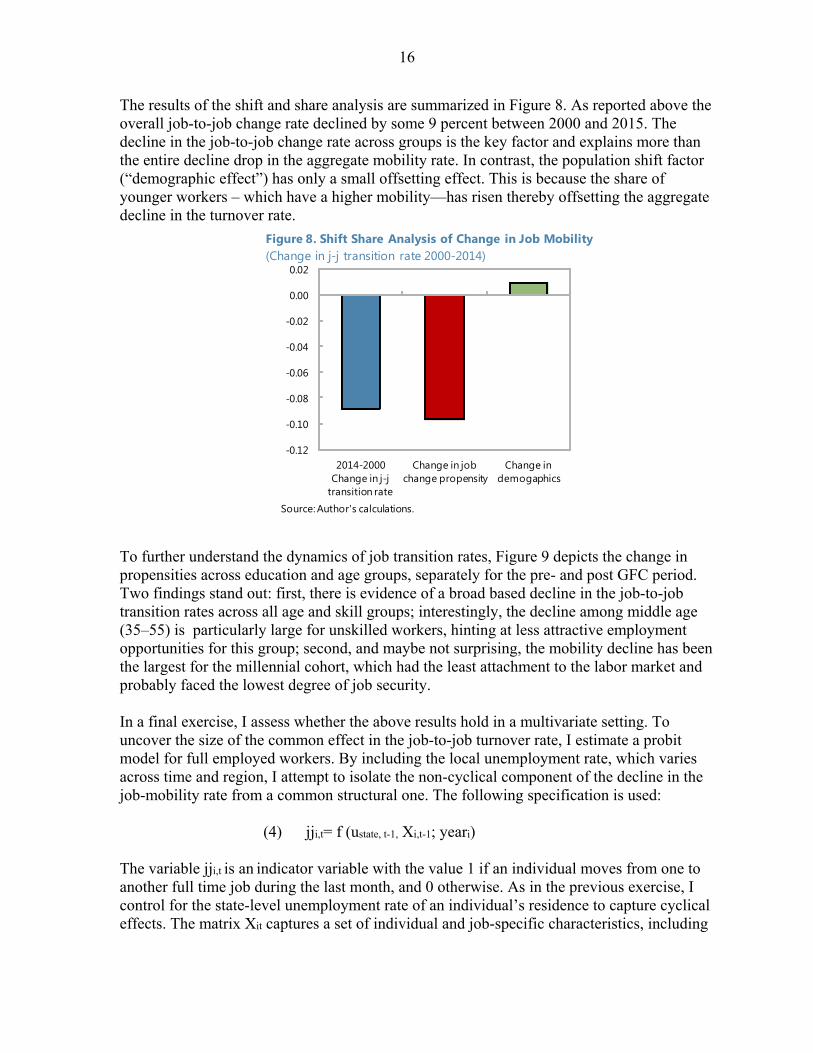
The results of the shift and share analysis are summarized in Figure 8. As reported above the overall job-to-job change rate declined by some 9 percent between 2000 and 2015. The decline in the job-to-job change rate across groups is the key factor and explains more than the entire decline drop in the aggregate mobility rate. In contrast, the population shift factor (“demographic effect”) has only a small offsetting effect. This is because the share of younger workers – which have a higher mobility—has risen thereby offsetting the aggregate decline in the turnover rate.

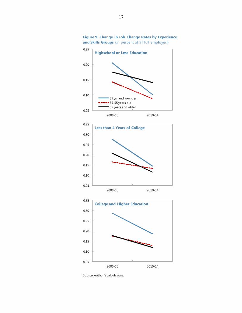
To further understand the dynamics of job transition rates, Figure 9 depicts the change in propensities across education and age groups, separately for the pre- and post GFC period. Two findings stand out: first, there is evidence of a broad based decline in the job-to-job transition rates across all age and skill groups; interestingly, the decline among middle age (35–55) is particularly large for unskilled workers, hinting at less attractive employment opportunities for this group; second, and maybe not surprising, the mobility decline has been the largest for the millennial cohort, which had the least attachment to the labor market and probably faced the lowest degree of job security. In a final exercise, I assess whether the above results hold in a multivariate setting. To uncover the size of the common effect in the job-to-job turnover rate, I estimate a probit model for full employed workers. By including the local unemployment rate, which varies across time and region, I attempt to isolate the non-cyclical component of the decline in the job-mobility rate from a common structural one. The following specification is used:

(4) jji,t= f (ustate, t-1, Xi,t-1; yeari) The variable jji,t is an indicator variable with the value 1 if an individual moves from one to another full time job during the last month, and 0 otherwise. As in the previous exercise, I control for the state-level unemployment rate of an individual’s residence to capture cyclical effects. The matrix Xit captures a set of individual and job-specific characteristics, including

-0.12

-0.10

-0.08

-0.06

-0.04

-0.02

0.00

0.02

2014-2000 Change in j-j

transition rate

Change in job change propensity

Change in demogaphics

Figure 8. Shift Share Analysis of Change in Job Mobility (Change in j-j transition rate 2000-2014)

Source: Author's calculations.

17

0.05

0.10

0.15

0.20

0.25

2000-06 2010-14

35 yrs and younger35-55 years old55 years and older

Highschool or Less Education

Figure 9. Change in Job Change Rates by Experienceand Skills Groups (In percent of all full employed)

Source: Author's calculations.

0.05

0.10

0.15

0.20

0.25

0.30

0.35

2000-06 2010-14

Less than 4 Years of College

0.05

0.10

0.15

0.20

0.25

0.30

0.35

2000-06 2010-14

College and Higher Education

18

years of work experience, education and other factors. The estimation results are reported in Table 3. The baseline model (column 1) shows that younger and more educated workers are churning more than others. Union members change less often, while city dwellers move more often between jobs. The results are by and large the same during the pre- and post GFC period (Table 3 columns 2–3). It is now possible to estimate whether after controlling for individual and job-specific variables, there remains evidence of a common effect. Estimates for a model which includes year dummies are reported in the final column. Figure 10 depicts the estimated marginal decline in the job-to-job transition probability with a 95 percent confidence interval captured by year dummies (columns 4). Marginal effects in the last column are computed as the average of individual year effects. The year dummies capture a growing negative effect. To assess by how much the decline in the job-to-job turnover rates is due to a common effect, I calculate the difference between the marginal effects of the year dummies in 2013/14 and 2001/02. This difference estimates at an annual turnover rate (≈0.003*12) explains about 4 percentage points of the 9 percentage point decline in the job-to-job transition rate. In comparison, the marginally higher unemployment rate in 2013/14 compared to 2001/02 explains only about 1.5 percentage points of the decline in the transition rate. Changes in the composition of the employed labor force and a lower propensity of younger workers to move jobs account for most of the remainder of the decline.

Identifying the underlying cause of the common component of the falling job turnover rate is beyond the scope of this paper. There is much speculation about whether lower market fluidity could be linked to lower wage growth or lower productivity. Establishing this link requires analysis of matched firm and employer data and should be a priority of future research.

-0.12

-0.10

-0.08

-0.06

-0.04

-0.02

0.00

0.02

0.04

2001 2003 2005 2007 2009 2011 2013

Figure 10. Decline in Job Change Rate Probability-(Marginal annual effect, Probit)

Source: Author's calculations. Last column in Table 3

19

IV. CONCLUSION

This paper has explored contributing factors to recent low average hourly wage growth in the U.S. The key findings are that the repair of the US labor market is not complete. The return of workers to the labor force is dampening wage growth. But there are also signs that the labor market is changing more fundamentally. For one, the wage-growth-Phillips curve appears to have flattened. The tightening of the labor market since 2010 has so far had not led to a measureable acceleration of wage growth, while it did so prior to the GFC. Finally, the widely documented decline in job turnover rates has continued. Specifically, job-to-job moves—a particular form of labor churning associated with higher wage growth—have fallen and the decline has been most pronounced for low-skilled workers who are moving less from job-to-job than before the GFC. These findings raise questions about the longer term prospects for healthy wage growth. In the near term, the closing of the employment gap could boost wage growth. But a return to persistently higher wage growth rates is uncertain. The flattening of the wage curve could be a sign that new jobs are of poorer quality and have low growth prospects. Although lower job market dynamism could be the result of better job-worker matching there is little supportive evidence in the literature so far. These leaves the possibility that lower turnover creates allocative inefficiencies leading to less productivity growth down the road. Direct evidence of economic costs is, however, scant. Further research on the determinants of labor market dynamism is urgently needed to understand its longer-term implications.

20

REFERENCES

Aaronson, D. and A. Jordan, 2014, “Understanding the Relationship Between Real Wage

Growth and Labor Market Conditions,” Chicago Fed Letter No. 327, October 2014. Acemoglu, Daron and David Autor, 2011, “Skills, Tasks and Technologies: Implications for

Employment and Earnings,” Handbook of Labor Economics, Vol. 4. Armenter Roc 2015, “A Bit of a Miracle No More: The Decline of the Labor Share”,

Philadelphia Federal Reserve Bank, Research Department. Balakrishnan, Ravi, Mai Dao, Juan Sole, and Jeremy Zook, 2015, “Recent U.S. Labor Force

Dynamics: Reversible or not?” IMF Working Paper No. 15/76 (Washington: International Monetary Fund).

Laurence Ball, 2014 Long-term damage from the Great Recession in OECD countries,

European Journal of Economics and Economic Policies: Intervention, Edward Elgar, vol. 11(2).

Carnevale, Anthony and Stephen Rose, 1998, Education for What? The New Office Economy (Princeton, N.J.: Educational Testing Service).

Daly, Mary C. and B. Hobijn March, 2015, Why Is Wage Growth So Slow? FRBSF

Economic Letter. Daly, Mary C. and B. Hobijn and Timothy Ni, 2013, The Path of Wage Growth and

Unemployment, FRBSF Economic Letter, July. Davis, Steven J. and John Haltiwanger, 2014, "Labor Market Fluidity and Economic

Performance," NBER Working Papers 20479 (Cambridge, Massachusetts: National Bureau of Economic Research).

Decker, Ryan A., John Haltiwanger, Ron S. Jarmin, and Javier Miranda, 2015, "Where Has

All The Skewness Gone? The Decline In High-Growth (Young) Firms In The U.S," NBER Working Papers 21776 (Cambridge, Massachusetts: National Bureau of Economic Research).

Dent, R., S. Kapon, F. Karahan, B. W. Pugsley, and A. Şahin, 2014, “The Long-Term

Unemployed and the Wages of New Hires,” Federal Reserve Bank of New York Liberty Street Economics, November 19.

Faberman R. Jason and Alejandro Justiniano 2015 “ Job Switching and Wage Growth”,

Chicago Fed Letter, Chicago Federal Reserve. Guzman, Jorge and Scott Stern, 2016, “The State of American Entrepreneurship: New

Estimates of the Quantity and Quality of Entrepreneurship for 15 US States, 1988-

21

2014,” NBER Working Paper No. 22095 (Cambridge, Massachusetts: National Bureau of Economic Research).

Higgins, P., 2014, “Using State-Level Data to Estimate How Labor Market Slack Affects

Wages,” Federal Reserve Bank of Atlanta Macro Blog, April 17. Hyatt, Henry R. and James R. Spletzer, 2013, The Recent Decline in Employment

Dynamics.US Census Bureau, Center for Economic Studies. Katz, Lawrence F. and Alan B. Krueger, 2016, The Rise and Nature of Alternative Work

Arrangements in the United States, 1995-2015. Krueger, Alan, 2015, “How Tight is the Labor Market?” The 2015 Martin Feldstein Lecture,

National Bureau of Economic Research. Kumar, Anil and Pia Orrenius, 2015, A Closer Look at the Phillips Curve Using State Level

Data, Dallas Fed, Working Paper No. 1409. Lazear, Edward P. and James Spelzer, 2012, “Hiring, Churn, and the Business Cycle”

American Economic Review Papers and Proceedings, Vol. 102, No 3, May 2012, pp. 575-579.

Mach, Traci L. and John A. Holmes, 2008, “The Use of Alternative Employment

Arrangements by Small Businesses: Evidence from the 2003 Survey of Small Business Finances,” Finance and Economics Discussion Series Divisions of Research & Statistics and Monetary Affairs, (Washington: Federal Reserve Board).

Molloy, Raven, Christopher L. Smith, Riccardo Trezzi and Abigail Wozniak, 2016,

“Understanding Declining Fluidity in the U.S. Labor Market,” Brookings Papers on Economic Activity, March 2016.

Robertson John, 2015, “No Wage Change?” Federal Reserve Bank of Atlanta, Macro Blog,

August 21. Rose, Stephen, 2015, “Beyond the Wage Stagnation Story Better Measures Show America’s

Workers Doing Better Than Previously,” (Washington: Urban Institute). Smith, C. L. 2014, “The Effect of Labor Slack on Wages: Evidence From State-Level

Relationships,” FEDS Notes, June 2, 2014. Solow, Robert, 2015, “The Future of Work: Why Wages Aren’t Keeping Up,” Pacific

Standard Blog, August 11. Starr, Evan and Norman Bishara, 2016 The Incomplete Noncompete Picture, Lewis & Clark

Law Review 497, 497–546.

22

Table 1 Wage level regression and change in local unemployment rate

(1) (2) (3) (4)

2000-15 2000-06 2009-15 2000-15

∆ U-rate (annual difference)-county 0.0086** 0.0042 0.0155**

(0.0035) (0.0063) (0.0064)

∆ U-rate county x 2000-06 0.0016

(0.0054)

∆ U-rate county x 2007-09 0.0127*

(0.0070)

∆ U-rate county x 2010-14 0.0131**

(0.0056)

U-rate county (t-1) -0.0072*** -0.0022 -0.0033 -0.0072***

(0.0027) (0.0066) (0.0065) (0.0027)

Years of schooling 0.0581*** 0.0605*** 0.0534*** 0.0581***

(0.0010) (0.0013) (0.0017) (0.0010)

Years of potential work experience 0.0223*** 0.0243*** 0.0209*** 0.0223***

(0.0007) (0.0010) (0.0012) (0.0007)

Years of potential work experience (sqrd) -0.0004*** -0.0004*** -0.0003*** -0.0004***

(0.0000) (0.0000) (0.0000) (0.0000)

Male 0.1223*** 0.1307*** 0.0986*** 0.1224***

(0.0050) (0.0067) (0.0088) (0.0050)

Caucasion 0.1038*** 0.1269*** 0.0675*** 0.1037***

(0.0057) (0.0076) (0.0101) (0.0057)

Urban dweller -0.0560 -0.0218 -0.1001 -0.0550

(0.0434) (0.0793) (0.1052) (0.0434)

Union member 0.1655*** 0.1592*** 0.1587*** 0.1655***

(0.0064) (0.0085) (0.0119) (0.0064)

Works in firm > 500 empl 0.0808*** 0.0796*** 0.0727*** 0.0808***

(0.0048) (0.0065) (0.0084) (0.0048)

Constant 1.6890*** 1.5064*** 1.7911*** 1.6906***

(0.0949) (0.1502) (0.1596) (0.0949)

Controls

Observations 29,562 15,928 10,038 29,565

R-squared 0.3477 0.3546 0.3758 0.3478

Standard errors in parentheses

*** p<0.01, ** p<0.05, * p<0.1

Log of hourl real wage rate

Industry, time and county dummies

23

Table 2. Wage Growth Phillips curve of full-time employed: 2000-14

(1) (2) (3) (4) (5) (6)2000-14 2000-14 2000-06 2010-14 2000-07 2010-14

Spline Spline

U-rate (t-12) -0.0029* -0.0079** 0.0017 -0.0162*** 0.0007

(0.0016) (0.0033) (0.0033) (0.0055) (0.0277)

U-rate (t-12) x 2000-06 -0.0053*

(0.0027)

U-rate (t-12) x 2007-09 -0.0037

(0.0033)

U-rate (t-12) x 2010-14 -0.0021(0.0017)

U Linear spline term 0.0178* 0.0010

(0.0095) (0.0281)

Years of schooling 0.0004 0.0005 -0.0011 0.0013 -0.0009 0.0013

(0.0010) (0.0010) (0.0015) (0.0018) (0.0015) (0.0018)

Years of potential work experience -0.0027*** -0.0027*** -0.0031*** -0.0027** -0.0031*** -0.0027**

(0.0006) (0.0006) (0.0009) (0.0011) (0.0009) (0.0011)

Years of potential work experience (sqrd) 0.0000*** 0.0000*** 0.0000** 0.0000* 0.0000** 0.0000*

(0.0000) (0.0000) (0.0000) (0.0000) (0.0000) (0.0000)

Constant 0.1786*** 0.1908*** 0.1938*** 0.0776 0.2273*** 0.0825(0.0375) (0.0393) (0.0603) (0.0786) (0.0628) (0.1577)

Observations 18,893 18,894 7,771 6,769 7,770 6,769

R-squared 0.0184 0.0186 0.0389 0.0688 0.0390 0.0688

Standard errors in parentheses

*** p<0.01, ** p<0.05, * p<0.1

Real Hour wage (annual growth rate)

24

Table 3 Probit analysis of Job-to-job change proensity full-time employed: 2000-14

(1) (2) (3) (4) (5)

2000-14 2000-06 2010-14 2000-14 2000-14

Marg eff

U-rate (t-12) -0.0321*** -0.0616** -0.0138 -0.0194 -0.0006

(0.0079) (0.0242) (0.0176) (0.0175)

Some college 0.0159 0.0329 -0.0138 0.0181 0.0006

(0.0344) (0.0473) (0.0609) (0.0345)

College + degree 0.0435 0.0311 0.0592 0.0492 0.0016

(0.0381) (0.0541) (0.0646) (0.0383)

Years of potential work experience -0.0177*** -0.0232*** -0.0125 -0.0181*** -0.0006

(0.0047) (0.0066) (0.0079) (0.0047)

Years of potential work experience (sqr 0.0003*** 0.0004*** 0.0002 0.0003*** 0.0000

(0.0001) (0.0001) (0.0002) (0.0001)

Urban dweller 0.1094*** 0.2084*** -0.0300 0.1021** 0.0030

(0.0395) (0.0659) (0.0615) (0.0403)

Union membership -0.0918*** -0.0998** -0.0876 -0.0969*** -0.0030

(0.0355) (0.0486) (0.0626) (0.0357)

Male 0.0642** 0.0528 0.0995* 0.0646** 0.0020

(0.0309) (0.0435) (0.0523) (0.0310)

White -0.0325 -0.0242 -0.0481 -0.0387 -0.0012

(0.0394) (0.0571) (0.0650) (0.0395)

Married 0.0016 -0.0129 -0.0150 -0.0001 0.0000

(0.0300) (0.0421) (0.0509) (0.0301)

Survey year = 2001 -0.0995 -0.0028

(0.0735)

Survey year = 2002 0.0048 0.0001

(0.0695)

Survey year = 2003 -0.2130*** -0.0054

(0.0818)

Survey year = 2004 -0.0926 -0.0026

(0.0785)

Survey year = 2005 -0.0965 -0.0027

(0.0756)

Survey year = 2006 -0.0554 -0.0016

(0.0716)

Survey year = 2007 -0.2253*** -0.0057

(0.0755)

Survey year = 2008 -0.2635*** -0.0064

(0.0773)

Survey year = 2009 -0.1263 -0.0035

(0.0797)

Survey year = 2010 -0.1298 -0.0035

(0.1134)

Survey year = 2011 -0.2228* -0.0056

(0.1183)

Survey year = 2012 -0.1414 -0.0038

(0.1071)

Survey year = 2013 -0.1485 -0.0040

(0.0984)

Survey year = 2014 -0.2243** -0.0056

(0.0929)

Constant -2.0911*** -2.0142*** -2.1451*** -2.0251*** …

(0.1843) (0.2858) (0.3334) (0.1989)

Observations 63,577 28,789 25,177 63,577 63,577

Standard errors in parentheses, Marginal effects are sample average of individual marginal effects

*** p<0.01, ** p<0.05, * p<0.1

Incidence of job-to-job transition

25

ANNEX 1

Variable definitions Real wage hourly wage rate of workers maid on an hourly basis

discounted by the CPI Real wage growth rate annual growth rate of real wage Years of schooling age – years of schooling needed to achieve the

reported education level – 6 Years of potential work experience age – years of schooling Job-to-job change indicator Binary variable with value of 1 if respondent with

full-time –full year employment reports a new employment within the last 4 weeks

Job changer (Figure 4) Binary variable with value of 1 if respondent was full-time- full employed worker with unchanged industry and occupation codes during last 12 months. Source CPS MORG

Sources: Current Population Survey and BLS

26

Table A1: Descriptive Statistics (CPS 2000-15) Obs Mean Std. Dev. Min Max Sample section II (B) Age 80,756 40.8 11.8 15 73 Male 80,756 0.5 0.5 0 1 Caucasian 80,756 0.8 0.4 0 1 Urban dweller 80,756 0.8 0.4 0 1 Married 80,756 0.6 0.5 0 1 Years of schooling 80,756 13.0 2.2 0 18 Years of pot work experience 80,756 21.8 11.9 1 49 Wage per hr (nominal) 80,756 15.6 8.2 3 88 Sample section II (C) Age 18,894 44.3 11.1 17 73 Male 18,894 0.6 0.5 0 1 Caucasian 18,894 0.9 0.4 0 1 Urban dweller 18,894 0.7 0.4 0 1 Married 18,894 0.6 0.5 0 1 Years of schooling 18,894 13.5 2.0 0 18 Years of pot work experience 18,894 24.7 11.3 1 49 Wage per hr (nominal) 18,894 19.0 9.6 3 98 Wage growth rate y/y real 18,894 0.1 0.6 -1 29 Unemployment rate (state of residence) 18,894 6.1 2.1 2 15 Sample section II (D) Age 63,577 42.8 11.4 16 73

Male 63,577 0.6 0.5 0 1

Caucasian 63,577 0.8 0.4 0 1

Urban dweller 63,577 0.7 0.4 0 1

Married 63,577 0.6 0.5 0 1

Years of schooling 63,577 13.8 2.1 0 18

Years of pot work experience 63,577 23.0 11.6 1 49

Job-to job change rate (annualized) 63,577 0.15 1.31 0 1 Sources: CPS; and Author's calculations